Hierarchical Learning of Hidden Markov Models with Clustering Regularization

Hui Lan1 Antoni B. Chan1

1Department of Computer Science, City University of Hong Kong, Kowloon Tong, Hong Kong

Abstract

Hierarchical learning of generative models is use-ful for representing and interpreting complex data.For instance, one application is to learn an HMMto represent an individual’s eye fixations on astimuli, and then cluster individuals’ HMMs todiscover common eye gaze strategies. However,learning the individual representation models fromobservations and clustering individual models togroup models are often considered as two separatetasks.In this paper, we propose a novel tree struc-ture variational Bayesian method to learn the indi-vidual model and group model simultaneously bytreating the group models as the parents of individ-ual models, so that the individual model is learnedfrom observations and regularized by its parents,and conversely, the parent model will be optimizedto best represent its children. Due to the regulariza-tion process, our method has advantages when thenumber of training samples decreases. Experimen-tal results on the synthetic datasets demonstrate theeffectiveness of the proposed method.

1 INTRODUCTIONThe hidden Markov model (HMM) [Rabiner, 1993] is an ef-fective method for statistically representing time series data,assuming that each observation in a sequence is generatedconditioned on a discrete state of a hidden Markov chain,i.e., a hidden state sequence. HMMs have been popularlyapplied in many areas that need to analyze time series data,such as speech recognition [Juang and Rabiner, 1991, Au-couturier and Mark, 2001], cognitive science [Chan et al.,2018, Hsiao et al., 2021b], and music analysis [Qi et al.,2007]. In particular, recent works using HMMs to modeleye fixation sequences has enabled interesting discoveriesabout the role of eye gaze in cognitive processes, includingthree processing states in information search tasks [Simolaet al., 2008], optimal strategies for face recognition [Chuk

et al., 2017b,a, An and Hsiao, 2021, Hsiao et al., 2021a],masking effects in visual search [Hsiao et al., 2021b], andthe association of eye gaze patterns to cognitive decline[Chan et al., 2018], emotion recognition [Zhang et al., 2019,Chan et al., 2020a], chronic pain [Chan et al., 2020c,b], anddecision making [Chuk et al., 2020].

The previous methods of hierarchical modelling of HMMslearn sequentially; first the individual models are learnedfrom observations, then the group models are learned fromthe individual models, as shown in Fig. 1(a). IndividualHMMs can be learned from observations using two typicalmethods: 1) the Baum-Welch (EM) algorithm [Baum et al.,1970], which computes the maximum likelihood parame-ter estimation of the HMM; 2) variational Bayesian EM(VBEM) algorithm [Beal et al., 2003], which computesthe posterior distribution over each parameter of HMMthrough maximizing the evidence lower bound (ELBO).Learning the group models is equivalent to clustering in-dividual HMMs, with each cluster center representing onegroup model. Coviello et al. [2014] proposed a variationalhierarchical EM (VHEM) algorithm, which clusters HMMsdirectly using their probability densities of the observationsequence, and estimates HMM cluster centers. Lan et al.[2021] proposed a variational Bayesian hierarchical EM(VBHEM) algorithm, a Bayesian version of VHEM.

In the above, the individual models and group models arelearned as separate tasks. When the data is sufficient, sep-arately learning individual and group models is fine, suchas experiments in [Coviello et al., 2014]. However, whenthe data is insufficient, the individual model may overfit,which affects the group model. For example, in face recog-nition [Chuk et al., 2014] or in scene perception Hsiao et al.[2021c], only one eye fixation sequence is tracked per stim-ulus. In this case, joint learning of individual and groupmodels will help learning of individual models throughpooling of common information in the group.

In this paper, we propose to estimate the individual and thegroup models simultaneously, as shown in Fig. 1(b), so that

Accepted for the 37th Conference on Uncertainty in Artificial Intelligence (UAI 2021).

(a) VBEM&VHEM (b) Ours

𝑌!

𝑌"

𝑌#

𝑌$

VBEM

VBEM

VBEM

VBEM

VHEM

VHEM

Aggregate

Aggregate

𝑌!

𝑌"

𝑌#

𝑌$

Sample

Sample

Sample

Sample

Sample

Sample

M (c) M (p) M (c) M (p)

Fig. 1: Illustration of the hierarchical modelling of HMMs, learning individual (child) models M (c) and group (parent) models M (p)

through: (a) VBEM and VHEM (sequentially); (b) Our method (simultaneously). {Yi}4i=1 represent 4 observation sequences. The HMMsare visualized by its 3 Gaussian emissions.

the group models can regularize the individual models. Thisis similar to the hierarchical generative process: 1) thereare group models; 2) individual models are sampled fromthe group models; 3) observations are sampled from theindividual models. This generative process is similar to topicmodel in document corpora, where documents are organizedin a multi-level hierarchy [Kim et al., 2013]. Although herewe focus on HMMs, the framework could be applied toother probabilistic models.

Our Contributions. In this paper, we propose a novel treestructure variational Bayesian method to learning the in-dividual models and group models simultaneously, wherethe group models are parents and the individual modelsare children. The group models regularize the individualmodels thereby alleviating overfitting of individual mod-els, and the group models are estimated from the individualmodels, thus iteratively affecting each other. In experiments,we obtain good clustering performance, and the individ-ual and group models are close to the ground-truth models,even for small sample size. Furthermore, the clustering isinherent in our model and does not resort to other existingclustering methods. Lastly, our child-parent framework is ageneric regularization method, and could be applied to otherprobabilistic models.

2 RELATED WORKHierarchical Models and Inference. In Fig. 1(b), the hier-archical HMMs structure allows us to use the group HMMsas the prior on the individual HMMs and then to learn theindividual HMMs. Dirichlet process (DP) provides nonpara-metric prior for the number of mixture components and iswidely considered in learning of HMMs. Teh et al. [2006]introduced the hierarchical Dirichlet process HMM (HDP-HMM) to learn an HMM, where each HMM state is repre-sented by a mixture model, and the mixture models in thedifferent groups share mixture components. Qi et al. [2007]utilized DP HMM mixture models (DP-H3M) to build anH3M for a song, where each HMM represents a song clip,i.e., the individual HMM is the same as one component of

the group H3M. In contrast, for our method, the mixturemodels do not share parameters, and each individual modelhas its own distribution that is not the same as one of thegroup models. The nested HDP [Paisley et al., 2014] is anovel prior to perform word-specific path clustering on ashared tree, which also has shared parameters and has notbeen applied to HMMs.

The HDP-HMM uses Markov chain Monte Carlo (MCMC)[Hastings, 1970, Gelfand and Smith, 1990] for posteriorinference. MCMC explores the parameter space relyingon sampling. However, when the model is complex (suchas the hierarchal HMM), performing Bayesian inferencevia MCMC can be exceedingly expensive. We resort tovariational Bayesian methods for inference on the individualmodels and group models. Variational inference (VI) is analternative to MCMC, which relies on optimization ratherthan sampling. For mixture models, VI may perform betterthan a more general MCMC technique (e.g., HamiltonianMonte Carlo), even for small datasets [Kucukelbir et al.,2015]. Zhang et al. [2016] derived a VI for the HDP-HMM.

Regarding VI, the hierarchical structure of priors has beenintroduced to relax the mean-field assumption of variationaldistributions, e.g., hierarchical variational models (HVMs)[Ranganath et al., 2016] and Ladder-VAE [Sønderby et al.,2016]. HVM is a two-level model that first draws variationalparameters from a prior and then draws latent variables fromthe corresponding likelihood. In this perspective, our modelis a three-level model since we also have a hyper-prior overvariational parameters, i.e., p(Mp). Also, Bouchacourt et al.[2018] developed a multi-level variational autoencoder (ML-VAE) for learning a disentangled representation of a set ofgrouped observations. However, these works focus on thehierarchical structure of latent variables (or latent code),such as assignment variable, not on the model parameters,while our method focuses on the hierarchical structure ofthe model parameters.

Regularization via Clustering. In our model, the groupmodels are actually cluster centers when clustering the in-

dividual models, and the clustering regularizes the learningof individuals. The idea of using clustering as regulariza-tion has been explored in other domains. Pang et al. [2014]simultaneously regularized the between- and within-classscatter matrices to learn regularized linear discriminant anal-ysis. Price et al. [2021] proposed a penalized likelihoodframework for estimating the C precision matrices withcluster regularization. Cluster-based regularization has alsobeen of interest in semisupervised learning, active learning,transfer learning, and other areas of AI [Soares et al., 2012,Sellars et al., 2020, Hubert and Arabie, 1985, Zhao et al.,2019, Long et al., 2013]. Soares et al. [2012] proposed arobust algorithm, cluster-based regularization (ClusterReg)for semisupervised learning (SSL), which takes advantageof partitions resulting from a clustering algorithm, and usessuch information to regularize prediction. The method isalso extended to Ensemble Learning [Soares et al., 2017].Sellars et al. [2020] used clustering based regularization toimprove decision boundaries within a novel SSL frameworkcalled two-cycle learning. In contrast to these methods, ourmethod is a Bayesian generative model, where the cluster-ing is inherent in our model, and does not resort to otherexisting clustering methods.

Hidden Markov (Mixture) Model. We briefly review hid-den Markov models (HMMs) and the hidden Markov mix-ture model (H3M) [Smyth, 1997], and define the notationused in the paper. An H3M models a set of observation se-quences as samples from a group of K hidden Markov mod-els (HMMs), and is parameterized by M = {ωi,Mi}Ki=1,where Mi is the ith HMM and ωi is the correspondingmixture component weight. An observation sequence withlength τ is denoted by y = (y1, y2, ..., yτ ), and depends on ahidden state sequence x = (x1, x2, ..., xτ ). The observationlikelihood for y ∼ M is p(y|M) =

∑i ωip(y|Mi), where

the ith HMM Mi with S states is specified by parametersMi = {πi, Ai, {Θi

k}Sk=1}. In detail, πi = [πi1, ..., πiS ] is

the initial state probability, where πik = p(x1 = k|Mi).Ai = [aik,k′ ]S×S is the state transition matrix, whereaik,k′ = p(xt+1 = k′|xt = k,Mi) is the transition probabil-ity from state k to k′. Θi

k is the parameter set of emissiondensity at state k. Here, we assume the emissions are Gaus-sian distributions, p(yt|xt = k,Mi) = N (yt|µik, (Λik)−1),with mean µik and precision matrix Λik.

3 METHODOLOGYIn this section, we introduce our tree structure variationalBayesian method based on HMMs. Our hierarchical modelconsists of the following generative process: 1) a parentH3M is sampled from a prior, with each HMM compo-nent corresponding to a group; 2) a child HMM is sam-pled around the parent model, specifically, via a distributionformed using the parent H3M parameters; 3) observationsare sampled from the child HMM. Here we use “parent” and“child” to refer to the group and individual models.

𝝅 ! ,#

𝑨 ! ,#

𝝁 ! ,#

𝜦 ! ,#

𝝎 !𝜂$(!)

𝛼$(!)

𝜀$(!)

𝑚$(!)

𝛽$(!)

𝑊$(!)

𝜈$(!)

𝑀#(!)

𝑀(!)

𝝅 ' ,(

𝑨 ' ,(

𝝁 ' ,(

𝜦 ' ,(

𝒁𝒊

𝜈$(') 𝛽$

(')

𝒙*(

𝒚*(

𝑛 ∈ [1,𝑁!]

𝑖 ∈ [1,𝐾(")]𝑀((')

𝑗 ∈ [1,𝐾($) ]

𝛼$(') 𝜀$

(')

𝛷

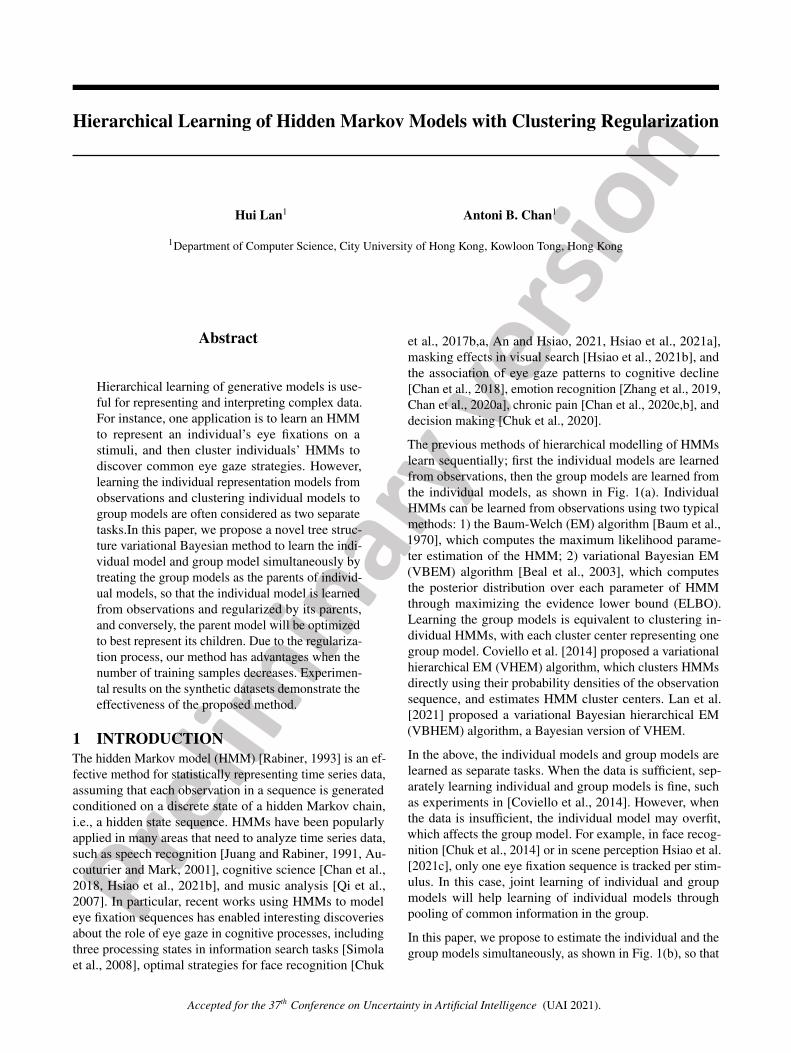
Fig. 2: Graphical model representation of our model. The solid lineplate denotes a set of i.i.d. samples. yin is an observation sequence,and xin is the state sequence that emits yin. Zi indicates theassignment of M (c)

i to an HMM component in M (p). The dashedline plate denotes an HMM: child HMM M

(c)i with parameters

{π(c),i, A(c),i, µ(c),i,Λ(c),i} and parent M (p)j with parameters

{π(p),j , A(p),j , µ(p),j ,Λ(p),j}. The variables outside the plate,{η(p)0 , α

(p)0 , ε

(p)0 ,m

(p)0 , β

(p)0 ,W

(p)0 , ν

(p)0 , α

(c)0 , ε

(c)0 , ν

(c)0 , β

(c)0 }

are hyperparameters, and Φ = {φi,j}K(c),K(p)

i=1,j=1 are a set of statepermutation matrices.

3.1 FRAMEWORK

Formally, consider a set of K(c) grouped samples Y ={Y1, Y2, . . . , YK(c)}, where Yi = {yi1, yi2, . . . , yiNi

} are

drawn from the ith child model M (c)i , and each sample

yin = (yin,1, yin,2, . . . , y

in,τ ) is a time series with length τ ,

and yin,t ∈ Rd. Each observation (or emission) yin,t at timet depends on the state of a discrete hidden variable xin,t, andthe sequence of hidden states xin = (xin,1, x

in,2, . . . , x

in,τ )

evolves as a first-order Markov chain. The hidden variablexin,τ can take one of S(c) values, i.e., xin,t ∈ {1, . . . , S(c)}.Each child model M (c)

i is an hidden Markov model (HMM)with S(c) states. The parent model M (p) is a hidden Markovmixture model (H3M) consisting of components M (p)

j ,

j ∈ {1, . . . ,K(p)}, K(p) ≤ K(c), and each M (p)j has S(p)

states, S(p) ≤ S(c). The child and parent are connectedthrough a child-parent distribution, from which the childmodel M (c)

i is sampled around the corresponding parentmodel M (p)

j . Note that we will always use superscripts (p)and (c) to distinguish the parameters for parent and childmodel, i and j to index the components in the mixturemodel of parents and children, and k and l to index thehidden states in the parent and child model, respectively.

An illustration of the probabilistic graphical model is shownin Fig. 2. Given the hyperparameters related to the parentmodel (e.g., α(p)

0 ), a parent model is sampled from its prior,i.e., M (p)

j ∼ p(M(p)j ), and weight ω(p) ∼ p(ω(p)) (the

hyperparameters are omitted to reduce clutter). Then, we in-troduce the assignment variable Zi, which takes one ofK(p)

values to assign the child model M (c)i to one of the com-

ponents in parent model, and the state permutation matrixφi,j , which has size S(c)×S(p), to match the states betweentwo HMMs M (c)

i and M (p)j . We assume the priors p(Zi =

j|ω(p)) = ω(p)j and p(φi,j) =

∏S(c)

k=1

∏S(p)

l=1 (1/S(p))φi,jk,l , re-

spectively. Given the assignment Zi = j, the generativeprocess of the data Yi is:

1. Sample a child model M (c)i ∼ p(M (c)

i |M(p)j );

2. Sample (i.i.d.) data sequences yin ∼ M(c)i , n =

1, ..., Ni.

Note that only the variables {yin}K(c),Ni

i=1,n=1 are observed. Allthe parameters (white circles) are unknown and are treatedas hidden variables. The child models are affected by obser-vations and parent models together, and the parent modelsare affected by the child models. Also, one child in ourmodel only has one parent, but one parent may have severalchildren, as shown in Fig. 2.

3.2 VARIATIONAL INFERENCEThe very large parameter space resulting from the hierarchi-cal HMM comes with a large computational burden. Thus,we resort to the variational Bayes, which is a faster alter-native to MCMC methods, to approximate the posteriordistributions of the hidden variables. First, we posit a familyof approximate densities q(·) ∈ Q over the hidden variables.Then, we find the member of that family that minimizesthe Kullback-Leibler (KL) divergence to the exact posterior.Finally, we approximate the posterior with the optimizedmember of the family q∗(·) [Blei et al., 2017].

ELBO. Formally, our goal is to find the best candidate in thefamily Q, i.e., the one closest in KL divergence to the exactposterior. Inference now amounts to solving the followingoptimization problem,

q∗(H) = arg minq(H)∈Q

KL(q(H)||p(H|Y )

), (1)

whereH = {M (p),M (c), Z,Φ, X} and the assumedQ canbe found in Sec. 3.4. Minimizing the KL divergence in (1) isequivalent to maximizing the evidence lower bound (ELBO)[Blei et al., 2017] as below (see Appendix A for details),

log p(Y ) ≥∑i

Eq(M(p))

[log p(Yi|M (p))

]−KL(q(M (p))||p(M (p)))

, L(M (p),M (c)),

where

L(M (p),M (c)) =∑i

Eq(M

(c)i )

[log p(Yi|M (c)

i )]

+∑i

∑j

zijEq(M(c)i )

Eq(M

(p)j )

[log p(M

(c)i |M

(p)j )

]+∑i

∑j

zijEq(ω(p))

[logω

(p)j

]+ Eω(p) log p(ω(p))

+∑j

Eq(M

(p)j )

[log p(M

(p)j )

]−∑i

∑j

zij log zij

−∑i

Eq(M

(c)i )

[log q(M

(c)i )]− Eq(ω(p))

[log q(ω(p))

]−∑j

Eq(M

(p)j )

[log q(M

(p)j )

], (2)

and zi,j = Eq(Z)[zij ]. The best child model M (c)∗ and the

best parent model M (p)∗ are obtained via{

M(p)∗ ,M

(c)∗}

= arg maxM(p),M(c)

L(M (p),M (c)).

It is important to note that although here we focus on HMMs,our framework could be used for any child and parent prob-ability distributions. The whole algorithm is summarizedin Alg. 1. We explain each step in the following subsec-tions, in particular the prior distributions and the variationaldistributions for approximating the posterior.

3.3 PRIORS DISTRIBUTIONS

Priors on Child Models. The key element in our ELBO in(2) is to construct the child-parent model p(M (c)

i |M(p)j ). It

can be considered as the prior on child model M (c)i given

assignment to parent model M (p)j , from which instances of

M(c)i are generated. Since M (c)

i and M (p)j are both HMMs

with their own states, a hidden state permutation matrix φi,j

has been introduced to match their states, where φi,jk,l = 1 if

the kth state in M (c)i corresponds to the lth state in M (p)

j ,otherwise φi,jk,l = 0. We assume that each child state k is

assigned to only one parent state l, i.e.,∑S(p)

l=1 φi,jk,l = 1,

∀k ∈ {1, ..., S(c)}, although multiple child states can beassigned to the same parent state.

With φi,j , we obtain a lower bound on log p(M(c)i |M

(p)j ),

log p(M(c)i |M

(p)j ) = log

∫p(M

(c)i , φi,j |M (p)

j )dφi,j

≥ Eq(φi,j)

[log p(M

(c)i |φ

i,j ,M(p)j )

]−KL(q(φi,j)||p(φi,j)),

where we introduce a variational posterior distributionq(φi,j). In the generative process, we assume that the statepermutation φi,j is applied to the parent model and then thechild model parameters (initial probability, transition matrix,and emission densities) are sampled. By marginalizing overthe state permutation matrix distribution q(φi,j), we avoidthe issue of multiple equivalent parameterizations of thehidden states.

Next, we construct the child-parent model, where the parentHMM parameters serve as the “mean” of the prior distribu-tions of the child HMM parameters,

log p(M(c)i |φ

i,j ,M(p)j ) = log p(π(c),i|α(c)

0 , φi,j , π(p),j)

+ log p(µ(c),i,Λ(c),i|φi,j , µ(p),j , β(c)0 ,Λ(p),j , ν

(c)0 )

+ log p(A(c),i|ε(c)0 , φi,j , A(p),j), (3)

where α(c)0 , ε(c)0 , β(c)

0 , and ν(c)0 are scalar hyperparametersto control the regularization effect from the parent models.Eq. 3 is the key that connects the parent model M (p)

j and

child model M (c)i . Specifically, we take the priors on the

child model parameters to be their corresponding conjugatepriors [Diaconis et al., 1979]:

1. Prior on ith child initial probabilities π(c),i,

p(π(c),i|α(c)0 , φi,j , π(p),j) = Dir(π(c),i|αi,j),

where αi,j=α(c)0 φi,jπ(p),j is a concentration hyperpa-

rameter, and φi,jπ(p),j is a state permutation of π(p),j .

2. Prior on ith child transition matrix A(c),i,

p(A(c),i|ε(c)0 , φi,j , A(p),j) =∏k

Dir(a(c),ik |εi,jk ),

where a(c),ik is the kth row of A(c),i, εi,j =

ε(c)0 φi,jA(p),j(φi,j)T is the concentration hyperparam-

eter of the kth row of the permuted matrix.

3. Priors on ith child emission mean and precision,

p(µ(c),i,Λ(c),i|φi,j , µ(p),j , β(c)0 ,Λ(p),j , ν

(c)0 )

=∏k

∏l

[N (µ

(c),ik |µ(p),j

l , (β(c)0 Λ

(c),ik )−1)

· W(Λ(c),ik |Λ(p),j

l /ν(c)0 , ν

(c)0 )]φi,j

k,l ,

whereW(·|W, ν) is a Wishart distribution with scalematrix W and degrees-of-freedom ν. With this prior,we have E[µ

(c),ik ] =

∑l φ

i,jk,lµ

(p),jl and E[Λ

(c),ik ] =∑

l φi,jk,lΛ

(p),jl .

Priors on Parent Models. Next, we consider the priors onparent models,

p(M (p)) = p(ω(p))

K(p)∏j=1

p(M(p)j ),

p(M(p)j ) = p(π(p),j)

S(p)∏l=1

p(a(p),jl )p(µ

(p),jl ,Λ

(p),jl ).

Similar to the child models, we assume conjugate priors onparent models parameters to simplify the analysis,

ω(p) ∼ Dir(ω(p)|η(p)0 ),

π(p),j ∼ Dir(π(p),j |α(p)0 ), a

(p),jl ∼ Dir(a

(p),jl |ε(p)0 ),

µ(p),jl |Λ(p),j

l ∼ N (µ(p),jl |m(p)

0 , (β(p)0 Λ

(p),jl )−1),

Λ(p),jl ∼ W(Λ

(p),jl |W (p)

0 , ν(p)0 ).

The hyperparameters η(p)0 , m(p)0 , W (p)

0 , α(p)0 , ε(p)0 , β(p)

0 , andν(p)0 are all scalars. Note that p(M (p)) serves as both the

prior on M (p) and the hyper-prior on M (c).

3.4 VARIATIONAL DISTRIBUTIONSThe ELBO in (2) is maximized via coordinating ascent w.r.t.the variational distribution over each hidden variable, i.e.,iteratively optimizing each factor, q(M (p)), q(M (c)), q(Z),q(Φ), and q(X), while holding the others fixed, resultingin the approximate posterior distributions for each hiddenvariable. Specifically, our method has two alternating steps:

1. Given q(M (p)) and q(M (c)), update q(X), q(Φ), andq(Z) via maximizing (2).

2. Update q(M (p)) and q(M (c)) via maximizing (2).

Here we restrict the family of distributions q(H) with amean field assumption, i.e., the q distribution factorizes w.r.t.each parameter. In the optimization, many of the parametershave closed form updates (similar to Beal et al. [2003]),while others need numeric solvers. We derive the optimalvariational distributions in the following.

3.4.1 Variational Distributions for Z, Φ, and X

We provide the optimal variational distributions for the as-signment variables Z, the state permutation matrices Φ, andthe hidden state sequences X . With the mean field assump-tion of variational distribution q, we are only interested inthe functional dependence of the RHS in (2) on the variablesZ, Φ, and X , respectively.

For the variational distribution q(Z) =∏i

∏j(zij)

zij and

log zij ∝ EM

(c)i

EM

(p)j

log p(M(c)i |M

(p)j ) + Eω(p) logω

(p)j .

After normalizing, the optimal solution is

zij =ω(p)j exp {E

M(c)i

EM

(p)j

log p(M(c)i |M

(p)j )}∑

l ω(p)l exp {E

M(c)i

EM

(p)l

log p(M(c)i |M

(p)l )}

, (4)

where ω(p)j = E[logω

(p)j ] and the expectation term is ap-

proximated by a lower bound (see Appendix B.1). zij isthe responsibility for the parent model M (p)

j explaining the

child model M (c)i and the corresponding observations Yi.

For the variational distribution q(Φ) =∏i

∏j q(φ

i,j),

q(φi,j) =∏k

∏l(φ

i,jk,l)

φi,jk,l , and thus E[φi,jk,l] = φi,jk,l. More-

over, we assume∑k φ

i,jk,l ≥ 1, which means at least one

state inM (c)i is assigned to the lth state inM (p)

j . There is noclosed form solution for φi,j and we solve for the optimalφi,j via the optimization problem

max L(φi,j) s.t.∑l

φi,jk,l = 1,∑k

φi,jk,l ≥ 1, (5)

where

L(φi,j) ∝ EM

(c)i

EM

(p)j

log p(M(c)i |M

(p)j ),

Algorithm 1 Co-learning M (p) and M (c)

Input: data Y = {Y1, Y2, . . . , YK(c)}, S(c), K(c), S(p),K(p), and hyperparameters α(c)

0 , ε(c)0 , β(c)0 , ν(c)0 , η(p)0 , m(p)

0 ,W

(p)0 , α(p)

0 , ε(p)0 , β(p)0 , ν(p)0 .

Output: M (p), M (c) and Z.1: Initialize M (p) and M (c).2: repeat3: for i = 1 to K(c) and j = 1 to K(p) do4: Compute φi,j via (5).5: Compute zij via (4).6: end for7: for each Yi, i = 1 to K(c) do8: Compute responsibilities rin,t,k and rin,t,k,k′ via

(6);9: Update M (c)

i : update α(c),ik , ε(c),ik,k′ , m

(c),ik , β(c),i

k ,

ν(c),ik , and W (c),i

k via (7), (8), and (9), respectively,for k = 1, ..., S(c).

10: end for11: Update M (p) via (11) and solving (12) and (13).12: until L(M (p),M (c)) converges.

which contains all terms in (2) involving φi,j (see AppendixB.2). φi,jk,l provides the probabilities of the kth child statecorresponding to the lth parent state.

For the variational distribution q(X) =∏i

∏n q(x

in), since

each xin is independent of the parent model, q(xin) can besolved using the traditional variational Bayesian EM forHMMs [Beal et al., 2003] given yin. The responsibilities

rin,t,k = E[xin,t,k], rin,t,k,k′ = E[xin,t,k′xin,t−1,k], (6)

k, k′ ∈ {1, . . . , S(c)}, are solved using the forward-backward algorithm. rin,t,k is the responsibility for the kth Gaussian for observation yin,t, and rin,t,k,k′ is a transitionresponsibility.

3.4.2 Variational Distributions for Child Models

With the conjugate priors of M (c) assumed in Sec. 3.3,q(M (c)) is determined automatically by optimization of thevariational distributions and has the same form as the priors(similar to Beal et al. [2003]). For q(M (c)

i ),

π(c),i ∼ Dir(π(c),i|α(c),i), a(c),ik ∼ Dir(a

(c),ik |ε(c),ik ),

µ(c),ik ∼ N (µ

(c),ik |m(c),i

k , (β(c),ik Λ

(c),ik )−1),

Λ(c),ik ∼ W(Λ

(c),ik |W (c),i

k , ν(c),ik ),

for i ∈ {1, · · · ,K(c)}, k ∈ {1, · · · , S(c)}. The parametersα(c),i, ε(c),ik , m(c),i

k , β(c),ik , W (c),i

k , ν(c),ik are all updated byclosed form solutions that combine observations and priors.

Specifically, for initial and transition probabilities,

α(c),ik = N i

1,k + α(c)0

∑j

zij∑l

φi,jk,lπ(p),jl , (7)

where on the RHS, N i1,k =

∑n r

in,1,k is the number of

observations in Yi with the kth state at t = 1, and the secondterm is the number of virtual samples provided by parentmodels with the kth state at t = 1 and π(p),j

l = E[π(p),jl ].

Similarly,

ε(c),ik,k′ = N i

k,k′ + ε(c)0

∑j

zij∑l

∑l′

φi,jk,la(p),ll,l′ φ

i,jk′,l′ , (8)

where N ik,k′ =

∑n

∑τt=2 r

in,t,k,k′ is the number of obser-

vations which transition from kth state to k′th state in thesequences, and the second term is the number of virtual sam-ples provided by parents models with the same transitionand a(p),ll,l′ = E[a

(p),ll,l′ ].

For the emission probability density, we have

m(c),ik = 1

β(c),ik

[β(c)0 mi

k +N ikyik

], (9)

β(c),ik = N i

k + β(c)0 , ν

(c),ik = N i

k + ν(c)0 ,

W(c),ik = N i

kSik +

Nikβ

(c)0

β(c),ik

(yik − mik)(yik − mi

k)T

+ β(c)0 Cik +

∑j

zij∑l

φi,jk,l

(β(c)0

β(p),jl

+ ν(c)0

)E[(Λ

(p),jl )−1

],

where

N ik =

∑n

∑t

rin,t,k, yik =1

N ik

∑n

∑t

rin,t,kyin,t,

Sik =1

N(i)k

∑n

∑t

rin,t,k(yin,t − yik)(yin,t − yik)T ,

mik =

∑j

zij∑l

φi,jk,lm(p),jl ,

Cik =∑j

zij∑l

φi,jk,l(m(p),jl − mi

k)(m(p),jl − mi

k)T ,

E[(Λ

(p),jl )−1

]= (W

(p),jl )−1/(ν

(p),jl − d− 1). (10)

The regularization effect of the parent model is seen in theupdate steps, where each update is a mix of observations(from data) and a regularization term (from parents). For ex-ample, in (9), m(c),i

k is updated by β(c)0 virtual samples mi

k

from parents and N ik observations yik which are assigned

to the ith child with kth state. β(c),ik and ν(c),ik are updated

by the number of observations assigned to the kth childstate N i

k plus the virtual samples size β(c)0 and ν(c)0 , respec-

tively. For W (c),ik , the first line is the same with VBEM,

and the second line shows the variance provided by theparent models. Note that, with the constraint

∑k φ

i,jk,l ≥ 1,

the regularization effect will not lose efficacy – even if N ik,

N ik,k′ and N i

1,k are all zeros for the kth state in child M (c)i ,

that state will not degenerate. Comparing with VBEM, ourmethod is equivalent to giving each parameter an exclusiveprior, and the prior is provided by its parent models andaveraged with weight zij φ

i,jk,l.

(a) τ=100 (b) τ=80 (c) τ=50 (d) τ=30 (e) τ=10

GT111111111222222222333333333

.36 .33 .31

.36 .20 .44

.37 .04 .59

.20 .55 .25

1

to 1

2

to 2

3

to 3

prio

r

111111111222222222333333333

1.0 .00 .00

1.0 .00 .00

1.0 .00 .00

1.0 .00 .00

1

to 1

2

to 2

3

to 3

prio

r

111111111222222222

333333333

.81 .18 .01

.84 .16 .00

.64 .36 .00

.00 .00 1.0

1

to 1

2

to 2

3

to 3

prio

r

111111111

222222222

333333333

.80 .00 .20

.47 .00 .53

.33 .33 .33

.74 .00 .26

1

to 1

2

to 2

3

to 3

prior

111111111

222222222

333333333

.50 .00 .50

.50 .00 .50

.33 .33 .33

.50 .00 .50

1

to 1

2

to 2

3

to 3

prio

r

111111111222222222333333333

.33 .34 .33

.32 .22 .46

.33 .06 .60

.18 .55 .27

1

to 1

2

to 2

3

to 3

prio

r

111111111222222222333333333

.72 .15 .13

.41 .28 .32

.44 .37 .18

.43 .22 .36

1

to 1

2

to 2

3

to 3

prio

r

111111111

222222222

333333333 1.0 .00 .00

1.0 .00 .00

.00 .04 .96

.00 .35 .65

1

to 1

2

to 2

3

to 3

prio

r

111111111

222222222

333333333 .94 .04 .02

1.0 .00 .00

.00 .04 .96

.00 .34 .66

1

to 1

2

to 2

3

to 3

prio

r

111111111222222222

333333333

.62 .01 .38

.00 .44 .56

.00 .51 .49

.69 .00 .31

1

to 1

2

to 2

3

to 3

prio

r

111111111

222222222333333333.51 .25 .25

1.0 .00 .00

.00 .50 .50

.00 .50 .50

1

to 1

2

to 2

3

to 3

prio

r

111111111222222222333333333

.63 .22 .15

.41 .28 .32

.40 .40 .20

.42 .19 .38

1

to 1

2

to 2

3

to 3

prio

r

111111111

222222222333333333 .58 .33 .10

.04 .72 .24

.44 .46 .10

.17 .35 .47

1

to 1

2

to 2

3

to 3

prio

r

111111111

222222222 333333333 .58 .42 .00

.04 .96 .00

.35 .65 .00

.77 .12 .12

1

to 1

2

to 2

3

to 3

prio

r

111111111

222222222

333333333 .84 .11 .05

1.0 .00 .00

.00 .04 .96

.00 .35 .65

1

to 1

2

to 2

3

to 3

prio

r

111111111

222222222

333333333 .50 .29 .21

1.0 .00 .00

.00 .04 .96

.00 .35 .65

1

to 1

2

to 2

3

to 3

prio

r

111111111

222222222

333333333 .55 .27 .18

1.0 .00 .00

.00 .05 .95

.00 .35 .65

1

to 1

2

to 2

3

to 3

prio

r

111111111

222222222333333333 .59 .37 .05

.04 .80 .16

.41 .51 .08

.14 .41 .45

1

to 1

2

to 2

3

to 3

prio

r

111111111

222222222333333333

.51 .38 .11

.53 .11 .36

.54 .42 .04

.57 .05 .38

1

to 1

2

to 2

3

to 3

prior

111111111222222222

333333333

.63 .36 .02

.91 .09 .00

.15 .42 .44

.88 .11 .00

1

to 1

2

to 2

3

to 3

prior

111111111

222222222

333333333

.88 .11 .01

1.0 .00 .00

.00 .79 .21

.00 .73 .27

1

to 1

2

to 2

3

to 3

prior

111111111222222222

333333333

.59 .36 .05

.91 .09 .00

.12 .42 .47

.88 .11 .01

1

to 1

2

to 2

3

to 3

prior

111111111

222222222

333333333

.91 .09 .00

1.0 .00 .00

.00 .80 .20

.00 .76 .24

1

to 1

2

to 2

3

to 3

prior

111111111

222222222333333333

.48 .36 .15

.53 .12 .35

.53 .42 .05

.57 .05 .38

1

to 1

2

to 2

3

to 3

prior

111111111

222222222

333333333

.48 .29 .23

.43 .38 .19

.23 .55 .22

.58 .11 .32

1

to 1

2

to 2

3

to 3

prior

111111111

222222222333333333

.71 .29 .00

.72 .28 .00

.45 .55 .00

.37 .31 .32

1

to 1

2

to 2

3

to 3

prior

111111111

222222222

333333333

.25 .08 .66

.71 .29 .00

.44 .56 .00

.00 .00 1.0

1

to 1

2

to 2

3

to 3

prior

111111111

222222222333333333

.44 .10 .46

.81 .15 .04

.24 .72 .04

.16 .37 .47

1

to 1

2

to 2

3

to 3

prior

111111111

222222222333333333

.75 .25 .00

.71 .29 .00

.45 .55 .00

.33 .33 .33

1

to 1

2

to 2

3

to 3

prior

111111111

222222222

333333333

.56 .28 .16

.51 .35 .14

.29 .55 .16

.69 .07 .24

1

to 1

2

to 2

3

to 3

prior

BV

EV

BB

EB

Ourp

VB 111111111222222222333333333

.33 .33 .33

.29 .27 .44

.35 .09 .56

.16 .62 .22

1

to 1

2

to 2

3

to 3

prior

111111111222222222333333333 .46 .40 .14

.20 .44 .36

.34 .35 .31

.44 .52 .04

1

to 1

2

to 2

3

to 3

prior

111111111222222222333333333

.37 .34 .30

.30 .25 .45

.35 .08 .57

.17 .60 .23

1

to 1

2

to 2

3

to 3

prior

111111111222222222333333333

.34 .33 .33

.33 .33 .33

.33 .33 .33

.33 .33 .33

1

to 1

2

to 2

3

to 3

prior

111111111222222222333333333

.35 .35 .30

.07 .66 .27

.46 .16 .38

.10 .59 .32

1

to 1

2

to 2

3

to 3

prior

111111111222222222333333333

.56 .26 .18

.34 .30 .36

.34 .43 .23

.37 .25 .38

1

to 1

2

to 2

3

to 3

prior

111111111

222222222 333333333 .56 .43 .01

.01 .98 .00

.33 .67 .00

.77 .12 .12

1

to 1

2

to 2

3

to 3

prior

111111111

222222222333333333.57 .29 .14

.00 1.0 .00

.33 .49 .17

.24 .74 .01

1

to 1

2

to 2

3

to 3

prior

111111111

222222222333333333 .57 .41 .02

.02 .85 .13

.37 .58 .05

.14 .36 .50

1

to 1

2

to 2

3

to 3

prior

111111111

222222222333333333

.33 .33 .33

.54 .11 .34

.53 .43 .04

.57 .04 .40

1

to 1

2

to 2

3

to 3

prior

111111111

222222222 333333333

.53 .43 .03

.83 .03 .14

.12 .51 .38

.26 .05 .69

1

to 1

2

to 2

3

to 3

prior

111111111222222222

333333333

.48 .13 .38

.55 .34 .11

.57 .39 .04

.53 .05 .43

1

to 1

2

to 2

3

to 3

prior

111111111

222222222

333333333

.66 .33 .01

.72 .27 .00

.49 .50 .00

.33 .33 .33

1

to 1

2

to 2

3

to 3

prior

111111111222222222333333333

.50 .41 .09

.48 .21 .32

.23 .02 .75

.46 .33 .21

1

to 1

2

to 2

3

to 3

prior

111111111

222222222

333333333

.44 .32 .24

.52 .36 .12

.27 .52 .21

.71 .06 .23

1

to 1

2

to 2

3

to 3

prior

EM

Ourc

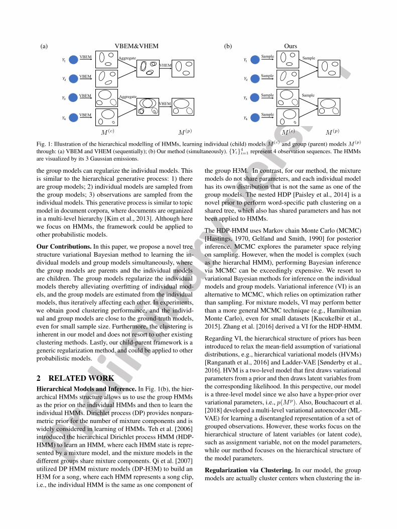
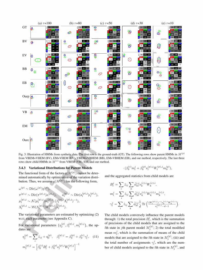
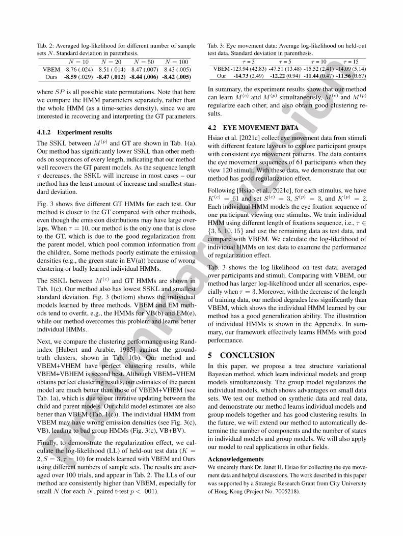
Fig. 3: Illustration of HMMs from synthetic data. The first row is the ground-truth (GT). The following rows show parent HMMs in M (p)

from VBEM+VHEM (BV), EM+VHEM (EV), VBEM+VBHEM (BB), EM+VBHEM (EB), and our method, respectively. The last threerows show child HMMs in M (c) from VBEM (VB), EM, and our method.

3.4.3 Variational Distributions for Parent ModelsThe functional form of the factors q(M (p)) cannot be deter-mined automatically by optimization of the variation distri-bution. Thus, we assume q(M (p)) has the following form,

ω(p) ∼ Dir(ω(p)|η(p)),

π(p),j ∼ Dir(π(p),j |α(p),j), a(p),jl ∼ Dir(a

(p),jl |ε(p),jl ),

µ(p),jl ∼ N (µ

(p),jl |m(p),j

l , (β(p),jl Λ

(p),jl )−1),

Λ(p),jl ∼ W(Λ

(p),jl |W (p),j

l , ν(p),jl ).

The variational parameters are estimated by optimizing (2)w.r.t. each parameter (see Appendix C).

For variational parameters {η(p)j , β(p),jl ,m

(p),jl }, the up-

dates are

η(p)j =

∑i

zij + η(p)0 , β

(p),jl = β

(p)0 + β

(c)0 γjl , (11)

m(p),jl =

[β(c)0 Bjl + β

(p)0 ν

(p),jl W

(p),jl

]−1

· (β(c)0 mj

l + β(p)0 ν

(p),jl W

(p),jl m

(p)0 ),

and the aggregated statistics from child models are

Bjl =∑i

zij∑k

φi,jkl ν(c),ik W

(c),ik ,

mjl =

∑i

zij∑k

φi,jkl ν(c),ik W

(c),ik m

(c),ik ,

γjl =∑i

zij∑k

φi,jkl1

dTr(

(W(p),jl )−1ν

(c),ik W

(c),ik

ν(p),jl −d−1

).

The child models conversely influence the parent modelsthrough: 1) the total precision Bjl , which is the summationof precisions of the child models that are assigned to thelth state in jth parent model M (p)

j ; 2) the total modifiedmean mj

l , which is the summation of means of the childmodels that are assigned to the lth state in M (p)

j ; (iii) andthe total number of assignments γjl , which are the num-ber of child models assigned to the lth state in M (p)

j , and

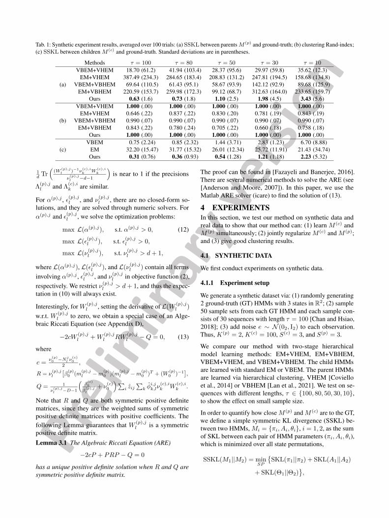
Tab. 1: Synthetic experiment results, averaged over 100 trials: (a) SSKL between parentsM (p) and ground-truth; (b) clustering Rand-index;(c) SSKL between children M (c) and ground-truth. Standard deviations are in parentheses.

Methods τ = 100 τ = 80 τ = 50 τ = 30 τ = 10

VBEM+VHEM 18.70 (61.2) 41.94 (103.4) 28.37 (95.6) 29.97 (59.8) 35.62 (12.3)EM+VHEM 387.49 (234.3) 284.65 (183.4) 208.83 (131.2) 247.81 (194.5) 158.68 (134.8)

(a) VBEM+VBHEM 69.64 (110.5) 61.43 (95.1) 58.67 (93.9) 142.12 (92.9) 89.68 (125.9)EM+VBHEM 220.59 (153.7) 259.98 (172.3) 99.12 (68.7) 312.63 (164.0) 233.65 (159.7)

Ours 0.63 (1.6) 0.73 (1.8) 1.10 (2.5) 1.98 (4.5) 3.43 (5.6)VBEM+VHEM 1.000 (.00) 1.000 (.00) 1.000 (.00) 1.000 (.00) 1.000 (.00)

EM+VHEM 0.646 (.22) 0.837 (.22) 0.830 (.20) 0.781 (.19) 0.843 (.19)(b) VBEM+VBHEM 0.990 (.07) 0.990 (.07) 0.990 (.07) 0.990 (.07) 0.990 (.07)

EM+VBHEM 0.843 (.22) 0.780 (.24) 0.705 (.22) 0.660 (.18) 0.758 (.18)Ours 1.000 (.00) 1.000 (.00) 1.000 (.00) 1.000 (.00) 1.000 (.00)

VBEM 0.75 (2.24) 0.85 (2.32) 1.44 (3.71) 2.83 (1.23) 6.70 (8.88)(c) EM 32.20 (15.47) 31.77 (15.32) 26.01 (12.34) 25.72 (11.91) 21.43 (34.74)

Ours 0.31 (0.76) 0.36 (0.93) 0.54 (1.28) 1.21 (1.18) 2.23 (5.32)

1d Tr

((W

(p),jl )−1ν

(c),ik W

(c),ik

ν(p),jl −d−1

)is near to 1 if the precisions

Λ(p),jl and Λ

(c),ik are similar.

For α(p),j , ε(p),jl , and ν(p),jl , there are no closed-form so-lutions, and they are solved through numeric solvers. Forα(p),j and ε(p),jl , we solve the optimization problems:

max L(α(p),j), s.t. α(p),j > 0, (12)

max L(ε(p),jl ), s.t. ε(p),jl > 0,

max L(ν(p),jl ), s.t. ν(p),jl > d+ 1,

where L(α(p),j), L(ε(p),jl ), and L(ν

(p),jl ) contain all terms

involving α(p),j , ε(p),jl , and ν(p),jl in objective function (2),respectively. We restrict ν(p),jl > d+ 1, and thus the expec-tation in (10) will always exist.

Interestingly, for W (p),jl , setting the derivative of L(W

(p),jl )

w.r.t. W (p),jl to zero, we obtain a special case of an Alge-

braic Riccati Equation (see Appendix D),

−2cW(p),jl +W

(p),jl RW

(p),jl −Q = 0, (13)

where

c =ν(p)0 −N

jl ν

(c)0

2 ,

R = ν(p),jl

[β(p)0 (m

(p),jl −m(p)

0 )(m(p),jl −m(p)

0 )T + (W(p)0 )−1

],

Q = 1

ν(p),jl −D−1

(β(c)0

β(p),jl

+ ν(c)0

)∑i zij

∑k φ

i,jk,lν

(c),ik W

(c),ik .

Note that R and Q are both symmetric positive definitematrices, since they are the weighted sums of symmetricpositive definite matrices with positive coefficients. Thefollowing Lemma guarantees that W (p),j

l is a symmetricpositive definite matrix.

Lemma 3.1 The Algebraic Riccati Equation (ARE)

−2cP + PRP −Q = 0

has a unique positive definite solution when R and Q aresymmetric positive definite matrix.

The proof can be found in [Fazayeli and Banerjee, 2016].There are several numerical methods to solve the ARE (see[Anderson and Moore, 2007]). In this paper, we use theMatlab ARE solver (icare) to find the solution of (13).

4 EXPERIMENTSIn this section, we test our method on synthetic data andreal data to show that our method can: (1) learn M (c) andM (p) simultaneously; (2) jointly regularize M (c) and M (p);and (3) give good clustering results.

4.1 SYNTHETIC DATA

We first conduct experiments on synthetic data.

4.1.1 Experiment setup

We generate a synthetic dataset via: (1) randomly generating2 ground-truth (GT) HMMs with 3 states in R2; (2) sample50 sample sets from each GT HMM and each sample con-sists of 30 sequences with length τ = 100 [Chan and Hsiao,2018]; (3) add noise e ∼ N (02, I2) to each observation.Thus, K(p) = 2, K(c) = 100, S(c) = 3, and S(p) = 3.

We compare our method with two-stage hierarchicalmodel learning methods: EM+VHEM, EM+VBHEM,VBEM+VHEM, and VBEM+VBHEM. The child HMMsare learned with standard EM or VBEM. The parent HMMsare learned via hierarchical clustering, VHEM [Covielloet al., 2014] or VBHEM [Lan et al., 2021]. We test on se-quences with different lengths, τ ∈ {100, 80, 50, 30, 10},to show the effect on small sample size.

In order to quantify how close M (p) and M (c) are to the GT,we define a simple symmetric KL divergence (SSKL) be-tween two HMMs, Mi = {πi, Ai, θi}, i = 1, 2, as the sumof SKL between each pair of HMM parameters (πi, Ai, θi),which is minimized over all state permutations,

SSKL(M1||M2) = minSP

{SKL(π1||π2) + SKL(A1||A2)

+ SKL(Θ1||Θ2)},

Tab. 2: Averaged log-likelihood for different number of samplesets N . Standard deviation in parenthesis.

N = 10 N = 20 N = 50 N = 100

VBEM -8.76 (.024) -8.51 (.014) -8.47 (.007) -8.43 (.005)Ours -8.59 (.029) -8.47 (.012) -8.44 (.006) -8.42 (.005)

where SP is all possible state permutations. Note that herewe compare the HMM parameters separately, rather thanthe whole HMM (as a time-series density), since we areinterested in recovering and interpreting the GT parameters.

4.1.2 Experiment resultsThe SSKL between M (p) and GT are shown in Tab. 1(a).Our method has significantly lower SSKL than other meth-ods on sequences of every length, indicating that our methodwell recovers the GT parent models. As the sequence lengthτ decreases, the SSKL will increase in most cases – ourmethod has the least amount of increase and smallest stan-dard deviation.

Fig. 3 shows five different GT HMMs for each test. Ourmethod is closer to the GT compared with other methods,even though the emission distributions may have large over-laps. When τ = 10, our method is the only one that is closeto the GT, which is due to the good regularization fromthe parent model, which pool common information fromthe children. Some methods poorly estimate the emissiondensities (e.g., the green state in EV(a)) because of wrongclustering or badly learned individual HMMs.

The SSKL between M (c) and GT HMMs are shown inTab. 1(c). Our method also has lowest SSKL and smalleststandard deviation. Fig. 3 (bottom) shows the individualmodels learned by three methods. VBEM and EM meth-ods tend to overfit, e.g., the HMMs for VB(b) and EM(e),while our method overcomes this problem and learns betterindividual HMMs.

Next, we compare the clustering performance using Rand-index [Hubert and Arabie, 1985] against the ground-truth clusters, shown in Tab. 1(b). Our method andVBEM+VHEM have perfect clustering results, whileVBEM+VBHEM is second best. Although VBEM+VHEMobtains perfect clustering results, our estimates of the parentmodel are much better than those of VBEM+VHEM (seeTab. 1a), which is due to our iterative updating between thechild and parent models. Our child model estimates are alsobetter than VBEM (Tab. 1(c)). The individual HMM fromVBEM may have wrong emission densities (see Fig. 3(c),VB), leading to bad group HMMs (Fig. 3(c), VB+BV).

Finally, to demonstrate the regularization effect, we cal-culate the log-likelihood (LL) of held-out test data (K =2, S = 3, τ = 10) for models learned with VBEM and Oursusing different numbers of sample sets. The results are aver-aged over 100 trials, and appear in Tab. 2. The LLs of ourmethod are consistently higher than VBEM, especially forsmall N (for each N , paired t-test p < .001).

Tab. 3: Eye movement data: Average log-likelihood on held-outtest data. Standard deviation in parenthesis.

τ = 3 τ = 5 τ = 10 τ = 15VBEM -123.94 (42.83) -47.51 (13.48) -15.52 (2.41) -14.09 (5.14)

Our -14.73 (2.49) -12.22 (0.94) -11.44 (0.47) -11.56 (0.67)

In summary, the experiment results show that our methodcan learn M (c) and M (p) simultaneously, M (c) and M (p)

regularize each other, and also obtain good clustering re-sults.

4.2 EYE MOVEMENT DATAHsiao et al. [2021c] collect eye movement data from stimuliwith different feature layouts to explore participant groupswith consistent eye movement patterns. The data containsthe eye movement sequences of 61 participants when theyview 120 stimuli. With these data, we demonstrate that ourmethod has good regularization effect.

Following [Hsiao et al., 2021c], for each stimulus, we haveK(c) = 61 and set S(c) = 3, S(p) = 3, and K(p) = 2.Each individual HMM models the eye fixation sequence ofone participant viewing one stimulus. We train individualHMM using different length of fixations sequence, i.e., τ ∈{3, 5, 10, 15} and use the remaining data as test data, andcompare with VBEM. We calculate the log-likelihood ofindividual HMMs on test data to examine the performanceof regularization effect.

Tab. 3 shows the log-likelihood on test data, averagedover participants and stimuli. Comparing with VBEM, ourmethod has larger log-likelihood under all scenarios, espe-cially when τ = 3. Moreover, with the decrease of the lengthof training data, our method degrades less significantly thanVBEM, which shows the individual HMM learned by ourmethod has a good generalization ability. The illustrationof individual HMMs is shown in the Appendix. In sum-mary, our framework effectively learns HMMs with goodperformance.

5 CONCLUSIONIn this paper, we propose a tree structure variationalBayesian method, which learn individual models and groupmodels simultaneously. The group model regularizes theindividual models, which shows advantages on small datasets. We test our method on synthetic data and real data,and demonstrate our method learns individual models andgroup models together and has good clustering results. Inthe future, we will extend our method to automatically de-termine the number of components and the number of statesin individual models and group models. We will also applyour model to real applications in other fields.

AcknowledgementsWe sincerely thank Dr. Janet H. Hsiao for collecting the eye move-ment data and helpful discussions. The work described in this paperwas supported by a Strategic Research Grant from City Universityof Hong Kong (Project No. 7005218).

References

Jeehye An and Janet H. Hsiao. Modulation of mood on eyemovement pattern and performance in face recognition.Emotion, 21(3):617–630, 2021.

Brian DO Anderson and John B Moore. Optimal control:Linear quadratic methods. Courier Corporation, 2007.

Jean-Julien Aucouturier and S Mark. Segmentation of musi-cal signals using hidden Markov models. In Proc. 110thConv. Audio Eng. Soc., 2001.

Leonard E Baum, Ted Petrie, George Soules, and NormanWeiss. A maximization technique occurring in the statis-tical analysis of probabilistic functions of Markov chains.The annals of mathematical statistics, 41(1):164–171,1970.

Matthew James Beal et al. Variational Algorithms for Ap-proximate Bayesian Inference. University of London,2003.

David M Blei, Alp Kucukelbir, and Jon D McAuliffe. Vari-ational inference: A review for statisticians. Journal ofthe American statistical Association, 112(518):859–877,2017.

Diane Bouchacourt, Ryota Tomioka, and SebastianNowozin. Multi-level variational autoencoder: Learningdisentangled representations from grouped observations.In Proceedings of the AAAI Conference on Artificial In-telligence, volume 32, 2018.

Antoni B Chan and Janet H Hsiao. EMHMM simulationstudy, 2018.

Cynthia YH Chan, Antoni B Chan, Tatia MC Lee, andJanet H Hsiao. Eye-movement patterns in face recogni-tion are associated with cognitive decline in older adults.Psychon. Bull. Rev., pages 1–8, 2018.

Frederick H.F. Chan, Tom J. Barry, Antoni B. Chan, andJanet H. Hsiao. Understanding visual attention to faceemotions in social anxiety using hidden Markov models.Cognition and Emotion, 34(8):1704–1710, 2020a.

Frederick H.F. Chan, Todd Jackson, Janet H. Hsiao, An-toni B. Chan, and Tom J. Barry. The interrelation betweeninterpretation biases, threat expectancies and pain-relatedattentional processing. European Journal of Pain, 24(10):1956–1967, 2020b.

Frederick H.F. Chan, Hin Suen, Janet H. Hsiao, Antoni B.Chan, and Tom J. Barry. Interpretation biases and visualattention in the processing of ambiguous information inchronic pain. European Journal of Pain, 24(7):1242–1256, 2020c.

Tim Chuk, Antoni B Chan, and Janet H Hsiao. Under-standing eye movements in face recognition using hiddenMarkov models. J. Vision, 14(11):8–8, 2014.

Tim Chuk, Antoni B. Chan, and Janet H. Hsiao. Is havingsimilar eye movement patterns during face learning andrecognition beneficial for recognition performance? Evi-dence from hidden Markov modeling. Vision Research,141:204–216, 2017a.

Tim Chuk, Kate Crookes, William G. Hayward, Antoni B.Chan, and Janet H. Hsiao. Hidden Markov model analysisreveals the advantage of analytic eye movement patternsin face recognition across cultures. Cognition, 169:102–117, 2017b.

Tim Chuk, Antoni B. Chan, Shinsuke Shimojo, and Janet H.Hsiao. Eye movement analysis with switching hiddenMarkov models. Behavior Research Methods, 52:1026–1043, 2020.

Emanuele Coviello, Antoni B. Chan, and Gert R. G. Lanck-riet. Clustering hidden Markov models with variationalHEM. J. Mach. Learn. Res., 15(1):697–747, January2014. ISSN 1532-4435.

Persi Diaconis, Donald Ylvisaker, et al. Conjugate priorsfor exponential families. The Annals of statistics, 7(2):269–281, 1979.

Farideh Fazayeli and Arindam Banerjee. The matrix gen-eralized inverse Gaussian distribution: Properties and ap-plications. In Joint European Conference on MachineLearning and Knowledge Discovery in Databases, pages648–664. Springer, 2016.

Alan E Gelfand and Adrian FM Smith. Sampling-basedapproaches to calculating marginal densities. Journal ofthe American statistical association, 85(410):398–409,1990.

W Keith Hastings. Monte Carlo sampling methods usingMarkov chains and their applications. 1970.

Janet H. Hsiao, Jeehye An, Yueyuan Zheng, and Antoni B.Chan. Do portrait artists have enhanced face processingabilities? Evidence from hidden Markov modeling of eyemovements. Cognition, 211, 104616, 2021a.

Janet H. Hsiao, Antoni B. Chan, Jeehye An, Su-Ling Yeh,and Jingling Li. Understanding the collinear maskingeffect in visual search through eye tracking. PsychonomicBulletin & Review, 2021b. (in press).

Janet H Hsiao, Hui Lan, Yueyuan Zheng, and Antoni BChan. Eye movement analysis with hidden Markov mod-els (EMHMM) with co-clustering. Behavior ResearchMethods, 2021c.

Lawrence Hubert and Phipps Arabie. Comparing partitions.J. Classif., 2(1):193–218, 1985.

Biing Hwang Juang and Laurence R Rabiner. HiddenMarkov models for speech recognition. Technometrics,33(3):251–272, 1991.

Do-kyum Kim, Geoffrey Voelker, and Lawrence Saul. Avariational approximation for topic modeling of hierar-chical corpora. In International Conference on MachineLearning, pages 55–63. PMLR, 2013.

Alp Kucukelbir, Rajesh Ranganath, Andrew Gelman, andDavid M Blei. Automatic variational inference in Stan.arXiv preprint arXiv:1506.03431, 2015.

Hui Lan, Ziquan Liu, Janet H. Hsiao, Dan Yu, and Antoni B.Chan. Clustering hidden Markov models with variationalBayesian hierarchical EM. submitted, 2021.

Mingsheng Long, Jianmin Wang, Guiguang Ding, DouShen, and Qiang Yang. Transfer learning with graphco-regularization. IEEE Transactions on Knowledge andData Engineering, 26(7):1805–1818, 2013.

John Paisley, Chong Wang, David M Blei, and Michael IJordan. Nested hierarchical Dirichlet processes. IEEEtransactions on pattern analysis and machine intelligence,37(2):256–270, 2014.

Yanwei Pang, Shuang Wang, and Yuan Yuan. Learning reg-ularized lda by clustering. IEEE transactions on neuralnetworks and learning systems, 25(12):2191–2201, 2014.

Bradley S Price, Aaron J Molstad, and Ben Sherwood. Es-timating multiple precision matrices with cluster fusionregularization. Journal of Computational and GraphicalStatistics, pages 1–30, 2021.

Yuting Qi, John William Paisley, and Lawrence Carin.Dirichlet process HMM mixture models with applicationto music analysis. In 2007 IEEE International Conferenceon Acoustics, Speech and Signal Processing-ICASSP’07,volume 2, pages II–465. IEEE, 2007.

Lawrence Rabiner. Fundamentals of Speech Recognition.PTR Prentice Hall, 1993.

Rajesh Ranganath, Dustin Tran, and David Blei. Hierarchi-cal variational models. In International Conference onMachine Learning, pages 324–333. PMLR, 2016.

Philip Sellars, Angelica Aviles-Rivero, and Carola BibianeSchönlieb. Two cycle learning: Clustering based regu-larisation for deep semi-supervised classification. arXivpreprint arXiv:2001.05317, 2020.

Jaana Simola, Jarkko Salojärvi, and Ilpo Kojo. Using hid-den Markov model to uncover processing states fromeye movements in information search tasks. Cognitivesystems research, 9(4):237–251, 2008.

Padhraic Smyth. Clustering sequences with hidden Markovmodels. In Proc. NeurIPS, pages 648–654, 1997.

Rodrigo GF Soares, Huanhuan Chen, and Xin Yao. Semisu-pervised classification with cluster regularization. IEEEtransactions on neural networks and learning systems, 23(11):1779–1792, 2012.

Rodrigo GF Soares, Huanhuan Chen, and Xin Yao. Acluster-based semisupervised ensemble for multiclassclassification. IEEE Transactions on Emerging Topics inComputational Intelligence, 1(6):408–420, 2017.

Casper Kaae Sønderby, Tapani Raiko, Lars Maaløe,Søren Kaae Sønderby, and Ole Winther. Ladder vari-ational autoencoders. arXiv preprint arXiv:1602.02282,2016.

Yee Whye Teh, Michael I Jordan, Matthew J Beal, andDavid M Blei. Hierarchical Dirichlet processes. Journalof the american statistical association, 101(476):1566–1581, 2006.

Aonan Zhang, San Gultekin, and John Paisley. Stochasticvariational inference for the HDP-HMM. In ArtificialIntelligence and Statistics, pages 800–808. PMLR, 2016.

Jinxiao Zhang, Antoni B. Chan, Esther Y.Y. Lau, andJanet H. Hsiao. Individuals with insomnia misrecognizeangry faces as fearful faces due to missing the eyes: Aneye-tracking study. Sleep, 42(2):zsy220, 2019.

Kai Zhao, Jingyi Xu, and Ming-Ming Cheng. Regularface:Deep face recognition via exclusive regularization. InProceedings of the IEEE/CVF Conference on ComputerVision and Pattern Recognition, pages 1136–1144, 2019.