Embed Size (px)
Citation preview

ARRAY-BASED GENOME COMPARISON OF ARABIDOPSISECOTYPES USING HIDDEN MARKOV MODELS
Michael SeifertLeibniz Institute of Plant Genetics and Crop Plant Research, Corrensstr. 3, 06466 Gatersleben, Germany
Ali Banaei, Jens Keilwagen, Michael Florian Mette, Andreas HoubenLeibniz Institute of Plant Genetics and Crop Plant Research, Corrensstr. 3, 06466 Gatersleben, Germany
[email protected], [email protected],[email protected], [email protected]
Francois Roudier, Vincent ColotEcole Normale Superieure, Departement de Biologie, CNRS UMR8186, 46 rue d’Ulm, 75230 Paris cedex 05, France
[email protected], [email protected]
Ivo GrosseMartin Luther University, Institute of Computer Science, Von-Seckendorff-Platz 1, 06120 Halle, Germany
Marc StrickertLeibniz Institute of Plant Genetics and Crop Plant Research, Corrensstr. 3, 06466 Gatersleben, Germany
Keywords: Array-CGH, Comparative Genomics, Arabidopsis Ecotypes, Hidden Markov Model (HMM)
Abstract: Arabidopsis thaliana is an important model organism in plant biology with a broad geographic distributionincluding ecotypes from Africa, America, Asia, and Europe. The natural variation of different ecotypes isexpected to be reflected to a substantial degree in their genome sequences. Array comparative genomic hy-bridization (Array-CGH) can be used to quantify the natural variation of different ecotypes at the DNA level.Besides, such Array-CGH data provides the basics to establish a genome-wide map of DNA copy number vari-ation for different ecotypes. Here, we present a new approach based on Hidden Markov Models (HMMs) topredict copy number variations in Array-CGH experiments. Using this approach, an improved genome-widecharacterization of DNA segments with decreased or increased copy numbers is obtained in comparison to theroutinely used segMNT algorithm. The software and the data set used in this case study can be downloadedfrom http://dig.ipk-gatersleben.de/HMMs/ACGH/ACGH.html.
1 INTRODUCTION
The method of array-based comparative genomichybridization (Array-CGH) has been widely appliedto several genomes for studying deletions, insertions,and amplifications of DNA segments (Mantripragadaet al., 2004) including studies on Arabidopsis thaliana(Borevitz et al., 2003; Martienssen et al., 2005; Fanet al., 2007) an important model organism in plantbiology. Due to the broad geographic distributionof Arabidopsis thaliana ecotypes their the naturalvariation is expected to be reflected to a substan-tial degree in their genome sequences. The applica-tion of Array-CGH to these genomes allows to quan-tify the natural variation at the DNA level. The ob-
tained Array-CGH data provides basics to establisha genome-wide map of DNA copy number variationsbetween different ecotypes. Based on such a map,future studies of DNA-histone interactions, histonemodifications, or transcript profiling will allow an im-proved comparison of different ecotypes.One important bioinformatics tasks is to create agenome-wide map characterizing regions of DNAcopy number variations in Array-CGH data of dif-ferent ecotypes. In recent years, the prediction ofDNA copy number variations in tumor data has re-ceived most attention, leading to the developmentof many different approaches for determining copynumber variations in Array-CGH data. These ap-proaches include genetic local search algorithms
(Jong et al., 2004), adaptive weights smoothing,(Hupe et al., 2004), and Hidden Markov Models(HMMs) (Fridlyand et al., 2004; Marioni et al., 2006;Cahan et al., 2008). Contributions to the comparisonof different approaches have been made by two recentstudies (Lai et al., 2005; Willenbrock and Fridlyand,2005).The basic concept of applying HMMs to the anal-ysis of Array-CGH data was initially developed by(Fridlyand et al., 2004). In this paper, we proposea new method based on HMMs for the detectionof DNA segments with decreased or increased copynumbers from Array-CGH data. This approach hasthe following features: (i) we use a three-state HMMpartitioning DNA segments into segments of de-creased, unchanged, or increased copy numbers, (ii)we incorporate a priori knowledge into the trainingof the HMM, and (iii) we use permuted Array-CGHdata to score predicted DNA segments with decreasedor increased copy numbers. We apply this HMM ap-proach to Array-CGH data of Arabidopsis thalianaecotypes from whole-genome NimbleGen tiling ar-rays. We obtain an improved genome-wide map ofcopy number variations compared to the standardsegMNT algorithm (Roche NimbleGen, Inc., 2008)routinely used for this task.
2 METHODS
2.1 Array-CGH Data
For the Array-CGH-based genome comparison ofArabidopsis thaliana ecotypes C24 and Columbia,leaf tissue is used to extract the DNA. Then the DNAis sheared by sonication and resulting DNA segmentsare differentially color-labeled for each ecotype. Sub-sequently, these DNA segments are hybridized toNimbleGen tiling arrays representing the referencegenome of ecotype Columbia. The arrays are readout and further processed using the NimbleScan soft-ware (Roche NimbleGen, Inc.) resulting in normal-ized log-ratios ot = log2(It(C24)/It(Columbia)) forall tiles t of an array, where It(C24) and It(Columbia)are the intensities of tile t under the correspondingecotype. Based on information about the chromo-somal locations of all tiles of an array, we create anArray-CGH profile o = o1, . . . ,oT for each chromo-some where all log-ratios ot are represented in in-creasing order of their chromosomal positions. EachArray-CGH experiment consists of two independentarrays with tiles at slightly different chromosomal lo-cations. That is, for two adjacent tiles of a chromo-some spotted on one array there generally exists one
Den
sity
−4 −2 0 2 4
0.0
0.5
1.0
1.5
Log−Ratio
Den
sity
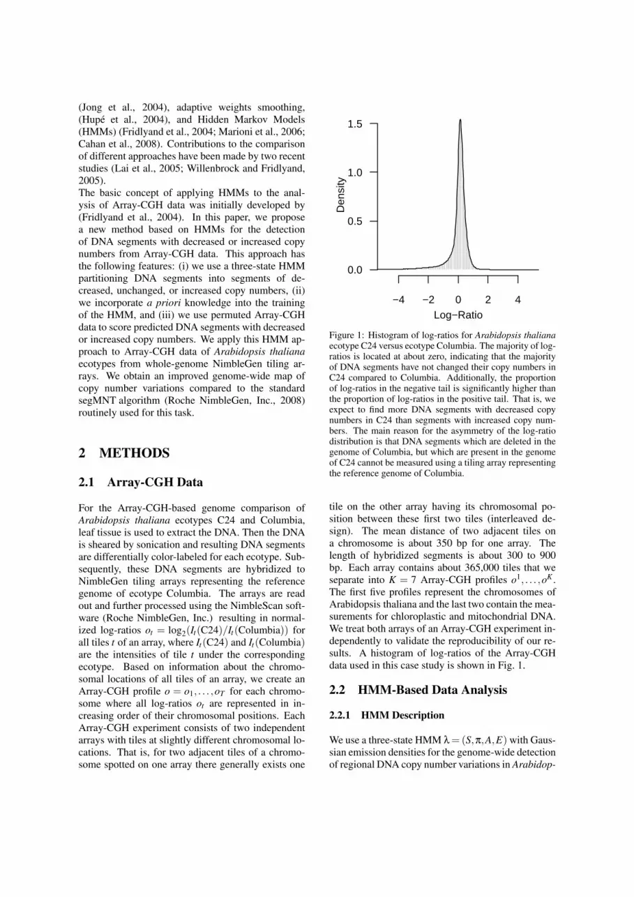
Figure 1: Histogram of log-ratios for Arabidopsis thalianaecotype C24 versus ecotype Columbia. The majority of log-ratios is located at about zero, indicating that the majorityof DNA segments have not changed their copy numbers inC24 compared to Columbia. Additionally, the proportionof log-ratios in the negative tail is significantly higher thanthe proportion of log-ratios in the positive tail. That is, weexpect to find more DNA segments with decreased copynumbers in C24 than segments with increased copy num-bers. The main reason for the asymmetry of the log-ratiodistribution is that DNA segments which are deleted in thegenome of Columbia, but which are present in the genomeof C24 cannot be measured using a tiling array representingthe reference genome of Columbia.
tile on the other array having its chromosomal po-sition between these first two tiles (interleaved de-sign). The mean distance of two adjacent tiles ona chromosome is about 350 bp for one array. Thelength of hybridized segments is about 300 to 900bp. Each array contains about 365,000 tiles that weseparate into K = 7 Array-CGH profiles o1, . . . ,oK .The first five profiles represent the chromosomes ofArabidopsis thaliana and the last two contain the mea-surements for chloroplastic and mitochondrial DNA.We treat both arrays of an Array-CGH experiment in-dependently to validate the reproducibility of our re-sults. A histogram of log-ratios of the Array-CGHdata used in this case study is shown in Fig. 1.
2.2 HMM-Based Data Analysis
2.2.1 HMM Description
We use a three-state HMM λ = (S,π,A,E) with Gaus-sian emission densities for the genome-wide detectionof regional DNA copy number variations in Arabidop-

sis thaliana ecotypes. The basis of this HMM is theset of states S = {−,=,+}. These states model thecopy number status of DNA regions in ecotype C24that is compared to the reference genome of ecotypeColumbia. Thus, state− corresponds to DNA regionswith decreased copy number, state = corresponds toDNA regions with unchanged copy number, and state+ corresponds to DNA regions with increased copynumber. The state of tile t is denoted by qt ∈ S. Weassume that a state sequence q = q1, ...,qT belongingto an Array-CGH profile o is generated by a homoge-neous Markov model of order one with (i) start distri-bution π = (π−,π=,π+), where πi denotes the prob-ability that the first state q1 is equal to i ∈ S, and (ii)stochastic transition matrix
A =
a−− a−= a−+a=− a== a=+a+− a+= a++
where ai j denotes the conditional probability thatstate qt+1 is equal to j∈ S given that state qt is equal toi∈ S. Clearly, the start distribution fulfills ∑i∈S πi = 1,and the transition probabilities of each state i ∈ S ful-fill ∑ j∈S ai j = 1. The state sequence is assumed to benon-observable, i.e. hidden, and the log-ratio ot of tilet is assumed to be drawn from a Gaussian emissiondensity, whose mean and standard deviation dependon state qt . We denote the vector of emission parame-ters by E = (µ−,µ=,µ+,σ−,σ=σ+) with mean µi ∈Rand standard deviation σi ∈R+ for the Gaussian emis-sion density
bi(ot) =1√
2πσiexp
(−1
2(ot −µi)2
σ2i
)of log-ratio ot given state qt = i ∈ S. An illustra-tion of the proposed HMM is given in Fig. 2. Sincewe have nearly equidistant tiles along a chromosomewith distances about 350 bp for adjacent tiles, we donot model chromosomal distances between adjacenttiles. Approaches that explicitly take adjacent dis-tances into account are e.g. BioHMM (Marioni et al.,2006) and RJaCGH (Rueda and Dıaz-Uriate, 2007).
2.2.2 HMM Initialization
In general, a good initial HMM should differentiateDNA regions of decreased or increased copy numbersfrom DNA regions of unchanged copy numbers withrespect to their log-ratios in the Array-CGH profile.Hence, a histogram of log-ratios, like in Fig. 1, helpsto find good initial HMM parameters. The choiceof initial parameters addresses the two realistic pre-sumptions. The first one is that the proportion of DNAregions with unchanged copy numbers is much higherthan that of DNA regions of decreased or increased
copy numbers. The second presumption is that thenumber of successive tiles with unchanged DNA copynumbers is also much higher than the number of suc-cessive tiles with decreased or increased DNA copynumbers. In this case study, we use π− = 0.2, π= =0.75, and π+ = 0.05 resulting in an initial start dis-tribution π = (0.2,0.75,0.05) where most weight isgiven to the state representing tiles with unchangedcopy number. Based on that, we choose an initial tran-sition matrix A with equilibrium distribution π. Thatis, we set the self-transition probability of state i ∈ Sto aii = 1− s/πi with respect to the scale parameters = 0.025 to control the state durations, and we useai j = (1− aii)/2 for a transition from state i to statej∈ S\{i}. We characterize the states by proper meansand standard deviations using initial emission param-eters µ− =−2.5, µ= = 0, µ+ = 1.5, σ− = 1, σ= = 1,and σ+ = 0.5. We refer to the initial HMM by λ1.
Figure 2: Three-state HMM with Gaussian emission densi-ties for the analysis of Array-CGH data. States of the HMMare represented by circles labeled with − (decreased), =(unchanged), and + (increased) modeling copy numbersof DNA segments in an ecotype compared to a referencegenome. Transitions between states are represented by ar-rows modeling all possible transitions in an Array-CGHprofile. Gaussian emission densities characterize the states.Thus, the emission density of the unchanged state (gray) hasits mean about zero, whereas the emission densities of thedecreased state (green) and the increased state (red) havemeans significantly different from zero.
2.2.3 HMM Prior
The incorporation of a priori knowledge is of primeimportance for training an HMM to predict biologi-cally relevant segments that vary in their copy num-bers between ecotypes. This can be realized using aprior distribution. We define the prior P[λ|Φ] of theHMM λ as a product of independent priors for eachtype of HMM parameters by
P[λ|Φ] = P[π|Φ] ·P[A|Φ] ·P[E|Φ].

We use a conjugate Dirichlet prior P[π|Φ] for start dis-tribution π defined by
P[π|Φ] = cπ ∏i∈S
πϑπ−1i
with positive hyper-parameter ϑπ ∈Φ and normaliza-tion constant cπ. The product of conjugate Dirichletpriors P[A|Φ] for transition matrix A is given by
P[A|Φ] = cA ∏i∈S
∏j∈S
aϑa−1i j
with positive hyper-parameter ϑa ∈Φ and normaliza-tion constant cA. We realize the prior for emissionparameters E using a product of conjugate Normal-Gamma priors
P[E|Φ] = ∏i∈S
P[µi|Φ] ·P[σi|Φ]
consisting of a state specific Gaussian density
P[µi|Φ] =√
εi√2πσi
exp(−εi
2(µi−ηi)2
σ2i
)as prior for mean µi with positive hyper-parametersηi ∈ Φ (a priori mean) and εi ∈ Φ (scale of a priorimean), and a state-specific Inverted-Gamma prior
P[σi|Φ] =2α
rii
Γ(ri)σ2ri+1i
exp(−αi
σ2i
)as prior for the standard deviation σi with positivehyper-parameters αi ∈ Φ (scale of standard devia-tion) and ri ∈ Φ (shape of standard deviation). Thechoice of this prior allows to include biological a pri-ori knowledge into the training of the HMM. As mo-tivated in Fig. 1, the integration of information aboutthe emission parameters of the HMM is important.Additionally, the used prior allows to determine ana-lytical parameter re-estimators for the HMM training.Especially, with the choice of the Normal-Gammadistribution as prior for a Gaussian emission density,we follow (Richardson and Green, 1997) transform-ing the proposed Gamma distribution as prior for theprecision σ
−2i into an Inverted-Gamma prior for the
standard deviation σi. With respect to the underlyingbiological question and motivated by the histogramof log-ratios in Fig. 1, we set the parameters of theNormal-Gamma priors to η− = −2.5, η= = 0, andη+ = 1.5 (a priori means). We use ε− = 10,000,ε= = 1,000 and ε+ = 7,500 (scale of a priori means),r− = 20,000, r= = 1, and r+ = 1,000 (shape of stan-dard deviations), and α− = α= = α+ = 10−4 (scaleof standard deviations), but in general this dependson the number of tiles in an Array-CGH experiment.
We ensure that the HMM can start in each state andthat all transitions are allowed by setting ϑπ = 10/3and ϑa = 10/9. The choice of these prior parametersensures a good characterization of the three HMMstates.
2.2.4 HMM Training
In most cases HMMs are trained by iteratively max-imizing the likelihood of the observation sequencesunder the model using the Baum-Welch algorithm(Baum, 1972; Rabiner, 1989; Durbin et al., 1998).This algorithm is part of the class of EM algorithms,which can be extended to include a priori knowledgeinto the iterative training by maximizing the posterior(Dempster et al., 1977). We train the initial HMMon all Array-CGH profiles using a maximum a pos-teriori (MAP) variant of the standard Baum-Welchalgorithm. That is, we iteratively obtain new HMMparameters
λh+1 = argmax
λ
(Q(λ|λh)+ log(P[λ|Φ])
)that maximize the posterior based on givenArray-CGH profiles O = (o1, . . . ,oK) and cur-rent HMM parameters λh. Here, Q(λ|λh) representsBaum’s auxiliary function (Rabiner, 1989; Durbinet al., 1998)
Q(λ|λh) =K
∑k=1
∑q∈STk
P[q|ok,λh] log(
P[ok,q|λ])
with complete data likelihood
P[o,q|λ] = πqt
T−1
∏t=1
aqt qt+1
T
∏t=1
bqt (ot)
of Array-CGH profile o and corresponding state se-quence q. The conflation of Q(λ|λh) and P[λ|Φ] en-ables us to include state-specific a priori knowledgeabout the parameters of Gaussian emission densitiesinto the training. Based on that, we use Lagrangemultipliers to determine the re-estimation formula foreach type of HMM parameters given by
πh+1i =
ϑπ−1+∑Kk=1 γk
1(i)|S|ϑπ−|S|+K
ah+1i j =
ϑa−1+∑Kk=1 ∑
T k−1t=1 εk
t (i, j)
|S|ϑa−|S|+∑Kk=1 ∑
T k−1t=1 γk
t (i)
µh+1i =
εiηi +∑Kk=1 ∑
T k
t=1 γkt (i) ·ok
t
εi +∑Kk=1 ∑
T kt=1 γk
t (i)
σh+1i =
√√√√∆i +∑Kk=1 ∑
T kt=1 γk
t (i) · (okt −µh+1
i )2
2ri +2+∑Kk=1 ∑
T kt=1 γk
t (i)

with ∆i = εi(µh+1i −ηi)2 +2αi. We calculate the prob-
abilities γkt (i) = P[qt = i|ok,λh] and εk
t (i, j) = P[qt =i,qt+1 = j|ok,λh] using the Forward-Backward al-gorithms for HMMs (Rabiner, 1989; Durbin et al.,1998). Starting with the initial HMM λ1 (h = 1), weiteratively determine new HMM parameters λh+1 andstop if the increase of the log-posterior of two succes-sive training iterations is less than 10−3.
●
●
●
●
●
●
●
●
●
●
●
●
●
●
●
●
●
●
●●
●
●
●
●
●
●
●
●
●
●
●
●
●
●
●
●
●
●●
●
●
●
●
●
●
●
●
●
●
●
●
●
●
●●
●
●
●
●
●
●
●●
●
●
●
●
●●
●●
●
●
●
●
●
●
●
●
●
●
●
●
●
●
●
●
●
●
●
●
●
●
●
●
●
●
●
●
●
●
●
●
●
●
●
●
●●
●
●
●
●
●
●
●
●
●
●
●
●
●
●
●●
●●
●
●
●
●
●
●
●
●
●
●
●
●●
●
●
●
●
●
●
●
●
●●
●
●
●
●
●
●
●
●
●
●
●
●
●
●
●
●
●
●
●
●
●
●
●
●
●
●
●
●
●
●
●●
●
●
●
●
●
●
●
●
●
●
●
●
●
●
●
●
●
●●
●
●●●
●
●
●●●
●
●
●
●
●
●
●
●
●
●
●
●
●
●●●
●
●●
●
●
●
●
●
●
●
●
●
●
●
●
●
●
●
●●
●
●
●
●
●
●●
●●
●
●
●
●●●
●
●
●
●
●
●
●
●
●
●
●
●
●
●●
●
●
●
●
●
●
●
●
●
●
●●
●●
●
●
●
●
●
●
●
●●
●
●
●
●●
●●●●
●
●
●
●
●
●
●
●
●
●
●
●
●
●
●
●
●
●
●●
●
●●
●
●
●
●
●●
●
●
●
●
●
●
●
●
●
●●●
●
●
●
●
●
●
●
●
●
●
●
●
●
●
●
●
●
●
●
●
●●
●
●
●
●
●
●
●●
●
●●
●
●
●
●
●
●
●●
●
●●
●●
●
●
●
●
●
●
●
●
●●
●
●
●
●
●
●●
●
●
●
●
●
●
●
●
●
●
●
●●
●
●
●
●
●
●
●
●
●
●
●●●
●
●●
●
●
●
●
●
●
●
●
●
●●
●
●
●
●
●
●
●
●
●
●
●
●●
●
●
●
●
●●
●
●
●
●
●
●
●
●
●
●
●
●
●
●
●
●
●
●
●
●
●
●
●
●
●
●
●
●
●
●
●
●
●
●
●
●
●
●
●
●
●
●
●●●
●
●
●●
●●
●
●
●
●
●
●●
●
●●
●
●
●
●
●
●
●
●
●
●
●
●●
●
●
●
●
●
●
●
●
●
●
●
●
●
●
●●
●
●
●
●
●
●●●
●
●
●
●
●
●
●
●
●
●●
●
●
●
●
●●●
●
●
●
●
●
●
●
●
●
●
●
●
●
●
●
●
●
●
●
●
●
●
●
●
●
●●
●
●●●
●
●
●
●
●
●
●
●
●
●
●
●●
●
●
●
●
●
●
●
●
●
●
●
●
●
●
●
●
●
●
●
●
●
●
●
●
●
●
●
●
●
●●
●
●
●
●
●
●
●
●
●
●
●
●
●
●
●
●
●
●
●
●
●
●
●
●
●
●
●
●
●
●
●
●
●
●
●
●
●
●●
●●
●
●
●
●
●●
●
●
●●
●
●
●
●
●
●
●
●
●
●
●
●
●
●
●
●
●
●
●
●
●
●
●
●
●
●
●
●
●
●
●
●
●
●●
●
●
●
●
●
●
●
●
●
●
●●
●
●
●●
●
●
●●
●●
●
●
●
●
●●●
●
●
●
●
●
●
●
●
●
●
●
●
●●
●
●
●
●
●●
●
●
●●
●
●
●
●
●
●
●
●
●
●
●
●
●
●
●
●
●
●
●
●
●
●
●
●
●
●
●●●
●
●
●
●
●
●
●
●
●
●
●
●
●
●
●
●
●
●●
●
●
●
●
●
●
●
●
●
●
●
●●
●
●
●
●●
●
●
●
●
●
●●
●
●
●
●●
●●
●
●●
●
●
●●
●
●
●
●
●
●
●
●
●
●
●
●
●
●
●
●
●
●
●
●
●
●
●
●
●●
●●
●
●
●
●
●
●
●
●
●
●
●
●
●
●
●●
●
●●
●
●
●
●
●
●
●
●
●
●
●
●
●
●
●
●●
●
●
●
●
●
●
●
●
●
●
●
●
●
●
●
●
●
●
●
●
●
●
●
●
●
●
●
●
●
●
●
●
●
●
●
●
●
●
●
●
●
●
●
●
●
●
●
●
●
●
●●
●
●●
●
●
●
●●
●
●
●
●
●
●
●●●
●
●
●
●
●
●
●
●●
●
●
●
●
●
●
●●
●
●
●
●
●
●
●
●
●
●
●
●
●
●
●●
●
●
●
●
●
●
●●
●
●
●
●
●
●
●
●
●
●
●
●●
●
●
●
●
●
●
●
●
●
●
●
●
●●
●
●
●
●
●
●●
●
●
●
●
●
●
●
●
●
●
●
●●
●
●
●
●
●
●
●
●●
●
●
●
●●
●
●
●
●
●
●●
●
●
●
●
●
●
●
●
●
●●
●
●
●
●
●
●●
●
●
●
●●●●
●
●
●●
●
●●●
●
●
●
●
●●
●
●
●
●
●●
●
●
●
●
●
●
●●
●
●
●
●
●
●
●
●
●
●
●
●
●
●
●
●
●
●
●
●
●
●
●
●
●
●
●
●
●
●
●
●
●
●●
●
●
●
●
●
●
●
●●
●
●
●
●
●●
●
●
●
●
●
●
●
●
●
●●
●
●
●
●●
●●
●
●
●●
●
●
●
●
●
●
●
●
●
●●
●
●●
●
●
●●
●
●●
●
●
●
●
●
●
●
●
●
●
●
●
●
●
●
●
●
●
●
●
●
●
●
●
●
●
●
●
●
●
●
●
●
●●
●●
●
●
●
●
●
●
●
●
●
●
●
●
●●
●
●
●
●
●
●
●●
●
●
●
●
●
●
●
●
●
●
●
●
●
●
●
●
●
●
●
●
●
●
●
●
●
●
●
●●
●
●
●
●●
●
●
●
●●
●●
●●
●
●
●
●
●
●
●
●
●
●
●
●
●●
●
●
●
●
●
●
●
●
●●●
●
●
●
●
●
●
●
●
●
●
●
●
●
●●
●
●
●
●
●●●●●
●
●
●
●
●
●
●
●●
●
●
●
●
●
●●
●
●
●
●
●
●
●
●
●
●
●●●
●
●
●
●
●
●
●
●
●
●
●
●
●
●●●
●●
●
●
●
●●
●
●
●
●
●
●●
●●
●
●
●
●
●
●
●
●●
●
●
●
●●
●
●●
●●
●
●
●●
●●●
●●
●
●
●
●
●
●
●
●
●
●
●
●●
●
●
●
●
●
●
●●
●
●
●
●
●
●
●
●
●●
●
●
●
●
●●
●●
●
●
●
●
●
●
●
●
●
●
●
●
●
●
●●
●●●
●
●
●●
●
●
●
●●
●
●●
●
●
●
●●
●
●
●
●
●
●
●
●
●
●
●
●●
●
●
●
●
●
●
●
●
●
●
●
●
●
●
●●
●
●●
●
●●
●
●●
●
● ●
●
●
1 2 3 4 5
−7
−5
−3
−1
Segment Length
Mea
n Lo
g−R
atio
●
●
●
●
●
●
●●
●
●
●●●
●●
●
●
●
●
●
●●
●●●
●●
●
●
●
●
●
●
●
●
●
●
●
●
●●
●●●
●●
●
●
●
●
●
●●
●
●●●●
●
●
●
●●
●●●
●
●●
●
●
●●
●
●
●
●
●
●
●
●
●●
●
●
●
●
●
●
●
●●●●
●
●●
●
●
●●
●
●
●
●●
●
●
●
●
●
●
●
●●
●
●
●
●
●
●
●
●
●
●
●
●
●
●●
●
●●
●
●●
●
●●
●
● ●
●
●●
Figure 3: Visualization of the scoring scheme for DNA seg-ments with decreased copy numbers. The red dot character-izes a DNA segment with segment length N = 3, mean log-ratio L =−2, and score S = N ·L =−6, which was predictedto have a decreased copy number status by the trained HMMin the original Array-CGH data. The red curve representsthe hyperbola f (n) = S/n of segment length n that dividesthe segments with decreased copy number status obtainedfrom the permuted Array-CGH profiles into segments withscores greater than −6, represented by black dots, and seg-ments with scores less or equal than−6, represented by graydots. The Score-value of the segment represented by the reddot is the proportion of gray dots in relation to the total num-ber of gray and black dots. Here, the Score-value is 0.088.
2.2.5 Segment Detection and Scoring
After the training of the initial HMM on allArray-CGH profiles, we apply the Viterbi algorithm(Rabiner, 1989; Durbin et al., 1998) to determine themost probable state sequence q for each Array-CGHprofile o. The so-called Viterbi path q partitionsthe corresponding Array-CGH profile into DNA seg-ments of decreased, unchanged, or increased copynumbers in relation to the reference genome se-quence. We refer to such a segment of copy number
status i ∈ S by
qtets (i) = qts , . . . ,qte
where the length of this segment is maximal (qts−1 6=i and qte+1 6= i for ts ≤ te), and all tiles within thissegment have the identical copy number status i (qt =i for each t ∈ [ts, te]). We score each segment by thesum of its log-ratios
S(qtets (i)|o) = Nte
ts ·Ltets =
te
∑t=ts
ot
to incorporate the segment length Ntets = te−ts +1 with
respect to the mean log-ratio Ltets = (1/Nte
ts )∑tet=ts ot
within the segment. Next, we determine the rele-vance of predicted DNA segments with decreased orincreased copy numbers. That is, we permute the log-ratios of each Array-CGH profile, and then, we applythe trained HMM to this data to predict DNA seg-ments with changed copy numbers that we score byS(qte
ts (i)|o). We repeat this step 100 times resulting intwo score distributions: one for DNA segments withdecreased copy numbers and another one for DNAsegments with increased copy numbers. The Score-value of a predicted segment in the original data is cal-culated by determining the proportion of scores underthe corresponding score distribution that are identicalor more extreme than the score of the considered seg-ment. DNA segments with a Score-value close to zeroare of most interest for our biologists. Fig. 3 shows anillustration of the scoring scheme.
3 Results and Discussion
With the aim of predicting DNA copy numbervariations between Arabidopsis thaliana ecotype C24and Columbia, we separately trained one HMM foreach of the two arrays of the Array-CGH experi-ment. Then, we used each trained HMM to de-termine DNA segments with decreased or increasedcopy numbers that we scored under permuted datafor obtaining segments of decreased or increased copynumbers at a Score-value level of 0.01. Alternatively,the standard service of Roche NimbleGen, Inc. in-cluded the segmentation of Array-CGH profiles us-ing their segMNT algorithm (Roche NimbleGen, Inc.,2008) resulting in two genome-wide segmentationprofiles. The first goal of the following study is toinvestigate where the predictions of the HMM ap-proach overlap and where they differ from those ofthe segMNT algorithm. The second goal is to char-acterize the prediction behavior of both methods forvarious levels of log-ratio signal intensities.

●●●●●●●●●●●●
●●●●●●●●●●●●●●●●●●
●
●●●●●●●
●●●●
●●●●●
●●●●●●●●
●●●●●●●
●
●
●●●●●●●●●●●●
●
●●●●●●
●●●●●●●●
●●
●●●●
●●
●●●
●●●●
●●
●
●●●●●
●
●●●
●●●●
●●●●●●●●●●●●●●●●●●●●●●
●●●●●
●●●
●●●●●●●●●●●●●●●●●●●●●
●
●●
●
●●●●●●●
●
●●●●●
●
●
●●●
●●●●●●
●
●●●●●●● ●
●●
●●●●●
●●●●●●●●
●
●●●●
●●
●●
●●●●●●●●●●●●●●
●●●●●
●
●
●●●●
●
●●●●●●●
●●●●
●●
●●
●●●●●●●
●
●
●
●●●●●●
●
●●
●
●●●●●●●
●●●
●●●●●●
●●●●
●
●●●●●●
●●●
●●●●●●
●
●●
●
●●●●●●
●
●●
●
●●●●●●
●
●●
●●●●●●●
●●
●
●●●●●●
●
●●
●
●●●●
●
●●●●●●
●
●●
●
●●●●●●
●
●●
●
●●●●●●
●
●●
●●●●●●●
●
●●●●●●●●●
●
●
●●
●●●●●
●●●●●●
●●
●
●●●
●●●●●●●●●●●●●●●●●●
●●●●●●●●
●●●●●●
●●●●●●●
●●●●●●●●●
●●
●●●●
●●●
●●●●●●● ●●●●●●●●●
●●●●●●●●●●●●●●●
●●●●●●●●●
●●●●●●●●●●●●●●●●
●●●●●●●●●●
●●●●●●
●●●●●●●●
●●●●●●
●
●
●●
●●●●
●●●●●●●●
●
●
●
●●●
●
●
●●●●●●●
●
●●●●●
●●●●●
●
●●
●
●
●●●●●●●●
●●●●●●●●●●
●●●●●●●●●●●●●
●●●●●●●●●●●●●●●●
●●●●●●●●●●●●●●●●●●●●●●●●●●●●●●●●●●●●●●●●
Log−
Rat
io
−6−4−2
024
Log−
Rat
ioHMM C24 vs. Col
●●●●●●●●●●●●
●●●●●●●●●●●●●●●●●●
●
●●●●●●●
●●●●
●●●●●
●●●●●●●●
●●●●●●●
●
●
●●●●●●●●●●●●
●
●●●●●●
●●●●●●●●
●●
●●●●
●●
●●●
●●●●
●●
●
●●●●●
●
●●●
●●●●
●●●●●●●●●●●●●●●●●●●●●●
●●●●●
●●●
●●●●●●●●●●●●●●●●●●●●●
●
●●
●
●●●●●●●
●
●●●●●
●
●
●●●
●●●●●●
●
●●●●●●● ●
●●
●●●●●
●●●●●●●●
●
●●●●
●●
●●
●●●●●●●●●●●●●●
●●●●●
●
●
●●●●
●
●●●●●●●
●●●●
●●
●●
●●●●●●●
●
●
●
●●●●●●
●
●●
●
●●●●●●●
●●●
●●●●●●
●●●●
●
●●●●●●
●●●
●●●●●●
●
●●
●
●●●●●●
●
●●
●
●●●●●●
●
●●
●●●●●●●
●●
●
●●●●●●
●
●●
●
●●●●
●
●●●●●●
●
●●
●
●●●●●●
●
●●
●
●●●●●●
●
●●
●●●●●●●
●
●●●●●●●●●
●
●
●●
●●●●●
●●●●●●
●●
●
●●●
●●●●●●●●●●●●●●●●●●
●●●●●●●●
●●●●●●
●●●●●●●
●●●●●●●●●
●●
●●●●
●●●
●●●●●●● ●●●●●●●●●
●●●●●●●●●●●●●●●
●●●●●●●●●
●●●●●●●●●●●●●●●●
●●●●●●●●●●
●●●●●●
●●●●●●●●
●●●●●●
●
●
●●
●●●●
●●●●●●●●
●
●
●
●●●
●
●
●●●●●●●
●
●●●●●
●●●●●
●
●●
●
●
●●●●●●●●
●●●●●●●●●●
●●●●●●●●●●●●●
●●●●●●●●●●●●●●●●
●●●●●●●●●●●●●●●●●●●●●●●●●●●●●●●●●●●●●●●●
Log−
Rat
io
●●
●
●●●●●●●
●●●●
●●●●●
●●●●●●●●
●●●●●●●
●
●
●●
●
●●●●●
●
●●●
●●●●
●●●
●●●●●●●●●●●●●●●●●●●●●
●
●●
●
●●●●●●●
●
●●
●●
●●●●●●●
●
●
●
●●●●●●
●
●●
●
●●●●●●●
●●●
●●●●●●
●●●●
●
●●●●●●
●●●
●●●●●●
●
●●
●
●●●●●●
●
●●
●
●●●●●●
●
●●
●●●●●●●
●●
●
●●●●●●
●
●●
●
●●●●
●
●●●●●●
●
●●
●
●●●●●●
●
●●
●
●●●●●●
●
●●
●●●●●●●
●
●●●●●●●●●
●
●
●●
●●●●●
●●●●●●
●●
●
●●●●●●
●
●
●●
●●●●
●●●●●●●●
●
●
●
●●●
●
●
●●●●●●●
●
●●●●●
●●●●●
●
●●
●
●
−6−4−2
024
Chromosomal Location
Log−
Rat
io
segMNT C24 vs. Col
Figure 4: Exemplary comparison of segmentation results for genome-wide selected DNA regions for ecotype C24 comparedto Columbia. From left to right separated by gray dashed lines: Region 1 [Chr1 2,779,800 bp - 2,806,847 bp], Region 2[Chr2 2,067,828 bp - 2,109,088 bp], Region 3 [Chr4 11,026,348 bp - 11,125,315 bp], and Region 4 [Chr4 13,596,032 bp -13,665,842 bp]. The top plot represents the segmentation results of the HMM approach. Green dots label tiles predicted by theHMM to have a decreased copy number. Red dots label tiles predicted by the HMM to have an increased copy number. Bluedashed lines highlight DNA segments significantly different from permuted data at a Score-value threshold of 0.01. Blackdots label tiles predicted by the HMM to have unchanged copy numbers. The bottom plot represents the segmentation resultsof the segMNT algorithm colored like the HMM segmentation. Both approaches provide a nearly identical segmentation ofthe displayed DNA regions.
3.1 Comparison of Segmentations
Based on the SignalMap viewer (Roche NimbleGen,Inc.), we performed a genome-wide inspection of thesegmentation results obtained by the HMM approachand by the segMNT algorithm. In practice, this basicstep allows a first direct comparison of both methods,and it provides a general overview of DNA regionswhere copy number variations have occurred. Bothapproaches predicted DNA segments with decreasedor increased copy numbers widely spread over thereference genome of Arabidopsis thaliana ecotypeColumbia. For the HMM approach we could quan-tify the proportion of these segments directly, becauseeach of these segments is assigned to one of the threeHMM states modeling the underlying copy number(Fig. 2). Considering the segMNT algorithm, thiswas not directly possible, because the obtained seg-ments are not grouped by copy number status. Thatis, the segMNT algorithm is only performing a seg-mentation of the Array-CGH profiles, but the pre-dicted segments are not categorized into segmentswith decreased, unchanged, and increased copy num-bers. Thus, we categorized all segments predictedby the segMNT algorithm with a mean log-ratio lessor equal than −0.5 as segments with decreased copynumbers, and in analogy, we labeled all segmentswith mean log-ratios greater or equal than 0.5 assegments with increased copy numbers. For a firstcomparison of segments that have been predicted byboth methods, we only count a segment predicted by
the HMM at a Score-value level of 0.01 as a seg-ment with decreased copy number if its correspond-ing mean log-ratio is less or equal than−0.5, and oth-erwise as a segment with increased copy number ifits mean log-ratio is greater or equal than 0.5. Thenumbers of predicted segments for each approach areshown in Tab. 1. DNA segments which are deletedin Columbia, but which exist in C24 cannot be mea-sured, because the tiling arrays represent the referencegenome of ecotype Columbia. Thus, it is expectedthat the small proportion of DNA segments with in-creased copy numbers is caused by this kind of ar-ray design (Fig. 1). The HMM approach identifiedsignificantly more DNA segments with decreased orincreased copy numbers than the segMNT algorithm.These numbers alone cannot be used to decide whichmethod should be preferred for the comparison ofArabidopsis thaliana ecotypes as also the lengthsof predicted segments, their chromosomal locations,and their reproducibility between both arrays shouldbe considered. To address this, we first analyzedthe overlap of segments predicted for both arrays byHMM or segMNT. The results are shown in Tab. 2. Ingeneral, both methods showed a good reproducibil-ity of their predicted segments. The higher num-ber of predicted segments by the HMM (Tab. 1) didnot lead to a great loss of reproducibility. That is,the HMM predicted more reproducible segments forboth arrays than the segMNT algorithm. Next, we in-vestigated how many of the segments that were pre-dicted by the segMNT algorithm have also been iden-

●
●
●
●
●●●●●●●●
●●
●
●●
●
●●
●
●
●●
●
●
●
●
●●
●
●
●●●
●●●
●●●
●●
●
●
●
●
●
●
●●●●●●
●●●●●
●
●●●●●●●●
●●●
●●●●●
●●●●●●
●●●●●
●●●●●
●●●●●●
●
●
●●
●●●
●●●
●
●
●●●
●
●
●●
●●
●●●●●●●●●
●●
●
●●
●●●●●
●●●
●●●●●●
●●●●●●
●●●●●●●●●●●●●●
●
●●●●●●
●●●●●
●●●●●●●●●
●●●●●
●●●●●●●●●
●
●●●●●●
●●●●●●●
●
●
●●●●
●
●●●●●●●●●●●
●●●●●●●
●●●●
●●●●
●●●
●
●●●
●●●●
●●●●●●●
●●
●●●●●●●●●●
●●●●
●●●●●
●●●●●●●●●●●
●●●
●●
●●●●●●●
●●●
●●●●
●●
●●●●●
●●●●
●●●●●●
●●●●
●●●●
●●●
●●
●
●
●
●
●
●●
●
●
●●●●●
●
●
●
●●
●
●●●●
●
●●●●●
●●
●
●
●
●
●
●
●
●●
●
●●●●
●●
●●●●●●
●●●
●●
Log−
Rat
io
−4
−2
0
2
Log−
Rat
ioHMM C24 vs. Col Array 1
●●
●
●●●●●●
●
●
●
●
●●●
●
●
●●●
●●
●●
●
●
●
●
●
●
●
●●
●
●
●
●
●●●
●
●
●
●
●
●
●
●
●●●●●●●
●●●
●●
●
●●●●
●
●●●●●●●●●●●
●●●●●●●
●●●●●●
●●
●
●●
●●●
●
●
●
●
●
●●●●
●
●
●
●
●
●
●
●
●
●
●
●
●●●●●●●●
●
●●● ●
●●●
●
●●●●●
●●●
●●●
●
●●●●●●●●●
●●●
●●●●●●●●
●●●●●●
●●●●●●●●●●●●●●●●●●●
●●●●●●●●●
●
●●●
●●●●●●●●
●●
●●●●●
●
●
●●
●●●●●●●●●
●●●●●●●●●●●
●
●●●
●
●●●
●●●●●●
●●●
●●●●●
●●●●●
●●●●●●●●●
●●●●●●●●
●
●●●●●●●●●
●●●●
●
●●●●●
●●●●
●●●●●
●
●●●●
●●●●●
●●
●
●●●●
●
●●
●●●●●●
●●
●
●
●
●
●
●
●
●
●
●
●
●●●●
●●
●
●
●●
●
●●
●
●
●●●●
●●●
●●
●●●●●
●
●
●
●
●
●
●●●●●●
●●●
●●
●●●
Log−
Rat
io
−4
−2
0
2
Log−
Rat
io
HMM C24 vs. Col Array 2
●
●
●
●
●●●●●●●●
●●
●
●●
●
●●
●
●
●●
●
●
●
●
●●
●
●
●●●
●●●
●●●
●●
●
●
●
●
●
●
●●●●●●
●●●●●
●
●●●●●●●●
●●●
●●●●●
●●●●●●
●●●●●
●●●●●
●●●●●●
●
●
●●
●●●
●●●
●
●
●●●
●
●
●●
●●
●●●●●●●●●
●●
●
●●
●●●●●
●●●
●●●●●●
●●●●●●
●●●●●●●●●●●●●●
●
●●●●●●
●●●●●
●●●●●●●●●
●●●●●
●●●●●●●●●
●
●●●●●●
●●●●●●●
●
●
●●●●
●
●●●●●●●●●●●
●●●●●●●
●●●●
●●●●
●●●
●
●●●
●●●●
●●●●●●●
●●
●●●●●●●●●●
●●●●
●●●●●
●●●●●●●●●●●
●●●
●●
●●●●●●●
●●●
●●●●
●●
●●●●●
●●●●
●●●●●●
●●●●
●●●●
●●●
●●
●
●
●
●
●
●●
●
●
●●●●●
●
●
●
●●
●
●●●●
●
●●●●●
●●
●
●
●
●
●
●
●
●●
●
●●●●
●●
●●●●●●
●●●
●●
Log−
Rat
io
−4
−2
0
2
Log−
Rat
io
segMNT C24 vs. Col Array 1
●●
●
●●●●●●
●
●
●
●
●●●
●
●
●●●
●●
●●
●
●
●
●
●
●
●
●●
●
●
●
●
●●●
●
●
●
●
●
●
●
●
●●●●●●●
●●●
●●
●
●●●●
●
●●●●●●●●●●●
●●●●●●●
●●●●●●
●●
●
●●
●●●
●
●
●
●
●
●●●●
●
●
●
●
●
●
●
●
●
●
●
●
●●●●●●●●
●
●●● ●
●●●
●
●●●●●
●●●
●●●
●
●●●●●●●●●
●●●
●●●●●●●●
●●●●●●
●●●●●●●●●●●●●●●●●●●
●●●●●●●●●
●
●●●
●●●●●●●●
●●
●●●●●
●
●
●●
●●●●●●●●●
●●●●●●●●●●●
●
●●●
●
●●●
●●●●●●
●●●
●●●●●
●●●●●
●●●●●●●●●
●●●●●●●●
●
●●●●●●●●●
●●●●
●
●●●●●
●●●●
●●●●●
●
●●●●
●●●●●
●●
●
●●●●
●
●●
●●●●●●
●●
●
●
●
●
●
●
●
●
●
●
●
●●●●
●●
●
●
●●
●
●●
●
●
●●●●
●●●
●●
●●●●●
●
●
●
●
●
●
●●●●●●
●●●
●●
●●●
Log−
Rat
io
−4
−2
0
2
Chromosomal Location
Log−
Rat
io
segMNT C24 vs. Col Array 2
Figure 5: Exemplary comparison of segmentation results for DNA regions on chromosome 4 for ecotype C24 compared toColumbia. From left to right separated by gray dashed lines: Region 1 [654,108 bp - 697,518 bp], Region 2 [1,305,320bp - 1,324,132 bp], Region 3 [3,731,013 bp - 3,761,229 bp], and Region 4 [5,411,025 bp - 5,433,126 bp]. The two top plotsrepresent segmentation results of the HMM approach for both interleaved arrays. Green dots label tiles predicted by the HMMto have a decreased copy number. Red dots label tiles predicted by the HMM to have an increased copy number. Blue dashedlines highlight DNA segments significantly different from permuted data at a Score-value threshold of 0.01. Black dots labeltiles predicted by the HMM to have unchanged copy numbers. The two bottom plots represent segmentation results of thesegMNT algorithm for both arrays. Red dashed lines show that no segmentation was obtained. Both approaches provide aquite different segmentation of the DNA regions. Here, the segMNT algorithm failed to identify segments with decreasedor increased copy numbers. The HMM approach clearly identifies segments with significantly decreased or increased copynumbers, and in addition, these biologically interesting results are reproducible for both arrays.
tified by the HMM. All segMNT segments of Tab. 1were also predicted by the HMM with respect toslightly varying segment start and end points. Thegeneral overlap between both approaches is exemplar-ily shown for selected DNA segments in Fig. 4. Ad-ditionally, Fig. 5 shows representative DNA regionswhere the HMM identified a copy number changereproducible for both interleaved arrays whereas thesegMNT algorithm failed.
3.2 Genome-wide Performance
The true copy number status of a predicted segmentcan be experimentally validated using independentmethods like PCR, sequencing, or insitu hybridiza-tion in the wet-lab. For thousands of identified seg-ments with putative copy number variations the usage
Table 1: Number of segments with decreased (−) and in-creased (+) copy numbers in ecotype C24 predicted byHMM and segMNT.
Array 1 Array 2Method − + − +HMM 1352 196 1427 205
segMNT 271 3 247 4
of such validation methods is currently not practical.In order to investigate how the prediction results ofthe segMNT algorithm and the HMM approach dif-fered at various log-ratio levels, we used a biolog-ically motivated model that defined the copy num-ber status of each tile with respect to its measuredlog-ratio. Based on the measurements of Array-CGHexperiments, segments with decreased copy numbers

HMM HMMsegMNT segMNT
0 0.02 0.04 0.06
0.5
1.0
1.5
2.0
2.5
3.0
3.5
4.0
0.00.2
0.40.6
0.81.0
FPR
TP
R
∆∆
●
●
●
●
●
●
●
●
●
●
●
●
●
●
●
●
●
●
●
●
●
●
●
●
0.00 0.01 0.02 0.03 0.04 0.05
0.0
0.2
0.4
0.6
0.8
1.0
FPR
TP
R
●●●
●
●
●
●
●
Figure 6: Prediction results obtained by segMNT and HMM at various log-ratio levels ∆ ∈ [0.5,4]. Left: FPR vs. TPR in thecontext of the variable log-ratio threshold ∆ defining the copy number of segments as being decreased or increased. Right:Top view on the left figure neglecting the log-ratio threshold.
Table 2: Number of reproducible segments between Array 1and Array 2 for HMM and segMNT based on predicted seg-ments of Tab. 1. Ai vs. A j: Segments predicted for Arrayi that are also predicted for Array j. Differences in countsresult mostly from segments predicted in one array that arepredicted in the other array by several non-overlapping seg-ments.
A1 vs. A2 A2 vs. A1Method − + − +HMM 1114 119 1209 129
segMNT 232 3 224 3
consist of tiles with log-ratios much less than zero,and segments with increased copy number are repre-sented by tiles with log-ratios much greater than zero(Fig. 1). For these reasons, we use a variable log-ratiothreshold ∆ ∈ R+ to define the copy number statusfor each tile in an Array-CGH profile. That is, a tilewith log-ratio ot is defined to have a decreased copynumber if its log-ratio ot is less or equal to the log-ratio threshold −∆, or conversely this tile is definedto have an increased copy number if its log-ratio ot isgreater or equal to the log-ratio threshold ∆. All tilesthat are not defined to have decreased or increasedcopy numbers are defined to have an unchanged copynumber. Based on that, we evaluated both segmen-tations, the one of the HMM at a Score-value level of0.01 and the other one of the segMNT algorithm fromthe previous section, against the segmentations ob-tained from systematically chosen variable log-ratiothresholds ∆ ∈ [0.5,4.0]. For each log-ratio thresh-old ∆ we determined the True-Positive-Rate TPR =TP/(TP+FN) and the FPR = FP/(FP+TN) of both
approaches. The results are shown in Fig. 6. In gen-eral, the HMM showed a much higher TPR than thesegMNT algorithm at a moderately higher FPR. Thisconfirms the previous findings: the HMM approachidentifies much more DNA segments with copy num-ber variations.
4 Conclusions
We introduced a three-state HMM approach(Fig. 2) for comparing the genomes of different eco-types of Arabidopsis thaliana. This approach is capa-ble of (i) incorporating biologically a priori knowl-edge into the training of model parameters, and of(ii) scoring DNA segments of decreased or increasedcopy numbers separately using permuted Array-CGHdata. We observed that our HMM approach identifiessignificantly more reproducible DNA segments withdecreased or increased copy numbers than the rou-tinely used segMNT algorithm. Using this HMM ap-proach, we find that about 5% of the genome of eco-type C24 shows decreased copy numbers and 0.3%shows increased copy numbers compared to the ref-erence genome of ecotype Columbia. Thus, we ob-tained a detailed map characterizing regions of DNAcopy number variations for future studies of eco-types including the analysis of DNA-histone interac-tions, histone modifications, and transcript profiling.Further biological interpretation of such a map canbe obtained using the AtEnsEMBL genome browser(James et al., 2007) for representing the map in thecontext of the genome annotation. In summary, all

results indicate that our HMM approach provides agood basis for Array-CGH-based genome comparisonof Arabidopsis thaliana ecotypes. One of our futureanalyses will focus on an in-depth comparison of theHMM approach against other available methods foranalyzing Array-CGH data.
ACKNOWLEDGMENTS
This work was supported by the Ministry of cul-ture Saxony-Anhalt grant XP3624HP/0606T and bythe DFG grant HO1779/7-2.
REFERENCES
Baum, L. E. (1972). An equality and associated max-imization technique in statistical estimation forprobabilistic functions of Markov processes. In-equalities, 3:1–8.
Borevitz, J. O., Liang, D., Plouffe, D., Chang, H.-S., Zhu, T., Weigel, D., Berry, C. C., Winzeler,E., and Chory, J. (2003). Large-scale identifica-tion of single-feature polymorphisms in complexgenomes. Genome Res, 13:513–523.
Cahan, P., Godfrey, L. E., Eis, P. S., Richmond, T. A.,Selzer, R. R., Brent, M., McLeod, H. L., Ley,T. J., and Graubert, T. A. (2008). wuHMM:a robust algorithm to detect DNA copy numbervariation using long oligonucleotide microarraydata. Nucleic Acids Research, 36(7):1–11.
Dempster, A., Laird, N., and Rubin, D. (1977). Max-imum likelihood from incomplete data via theEM algorithm. Journal of the Royal StatisticalSociety, Series B, 39(1):1–38.
Durbin, R., Eddy, S., Krogh, A., and Mitchision, G.(1998). Biological sequence analysis - Prob-abilistic models of proteins and nucleic acids.Cambridge University Press.
Fan, C., Vibranovski, M. D., Chen, Y., and Long,M. (2007). A Microarray Based Genomic Hy-bridization Method for Identification of NewGenes in Plants: Case Analyses of Arabidopsisand Oryza. J Integr Plant Biol, 49(6):915–926.
Fridlyand, J., Snijders, A. M., Pinkel, D., Albertson,D. G., and Jain, A. N. (2004). Hidden Markovmodels approach to the analysis of array CGHdata. J Multivariate Analysis, 90:132–153.
Hupe, P., Stransky, N., Thiery, J.-P., Radvanyi, F., andBarillot, E. (2004). Analysis of array CGH data:
from signal ratio to gain and loss of DNA re-gions. Bioinformatics, 20(18):3413–3422.
James, N., Graham, N., Celments, D., Schildknecht,B., and May, S. (2007). AtEnsEMBL: A Post-Genomic Resource Browser for Arabidopsis.Methods Mol Biol, 406:213–228.
Jong, K., Marchiori, E., Meijer, G., Vaar, A. v. d., andYlstra, B. (2004). Breakpoint identification andsmoothing of array comparative genomic hy-bridization data. Bioinformatics, 20(18):3636–3637.
Lai, W. R., Johnson, M. D., Kucherlapati, R., andPark, P. J. (2005). Comparative analysis ofalgorithms for identifying amplifications anddeletions in array CGH data. Bioinformatics,21(19):3763–3770.
Mantripragada, K. K., Buckley, P. G., de Stahl, T. D.,and Dumanski, J. P. (2004). Genomic microar-rays in the spotlight. Trends Genet, 20:87–94.
Marioni, J. C., Thorne, N. P., and Tavare (2006).BioHMM: a heterogeneous hidden Markovmodel for segmenting array CGH data. Bioin-formatics, 22(9):1144–1146.
Martienssen, R. A., Doerge, R. W., and Colot, V.(2005). Epigenomic mapping in Arabidopsis us-ing tiling microarrays. Chromosome Research,13:299–308.
Rabiner, L. (1989). A Tutorial on HiddenMarkov Models and Selected Applications inSpeech Recognition. Proceedings of the IEEE,77(2):257–286.
Richardson, S. and Green, P. J. (1997). On BayesianAnalysis of Mixtures with an Unknown Numberof Components. Journal of the Royal StatisticalSociety, Series B, 59(4):731–792.
Roche NimbleGen, Inc. (2008). A Performance Com-parison of Two CGH Segmentation Analysis Al-gorithms: DNACopy and segMNT. Availableonline: http://www.nimblegen.com.
Rueda, O. M. and Dıaz-Uriate, R. (2007). Flex-ible and Accurate Dection of Genomic Copy-Number Changes from aCGH. PLoS ComputBiol, 3(6).
Willenbrock, H. and Fridlyand, J. (2005). A compar-ison study: applying segmentation to array CGHdata for downstream analyses. Bioinformatics,21(22):4084–4091.