Multilevels Hidden Markov ModelsFor Temporal Data Mining

Weiqiang Lin1, Mehmet A. Orgun1, and Graham J. Williams2

1 Department of Computing, Macquarie University Sydney, NSW 2109, Australia, Email:fwlin, mehmetg@comp.mq.edu.au

2 CSIRO Mathematical and Information Sciences, GPO Box 664, Canberra ACT 2601,Australia, Email:fGraham.Williams g@cmis.csiro.au

Abstract. This paper describes new temporal data mining techniques for extracting in-formation from temporal health records consisting of time series of diabetic patients’treatments. In this new method, there are three steps for analyzing patterns from a lon-gitudinal data set. The first step, a structural-based pattern search, to find qualitativepatterns (or, structural patterns). The second step performs a value-based search to findquantitative patterns. In the third step we combine results from the first two steps toform new model. The hidden Markov model has the expressive power of both qualita-tive analysis and data quantitative analysis. The global patterns can therefore be identi-fied from a DTS set.

Keywords: temporal data mining, discrete-valued time series, similarity patterns, peri-odicity analysis, hidden Markov model

1 Introduction

Temporal data mining is concerned with discovering qualitative and quantitative tem-poral patterns in a temporal database or in a discrete-valued time series (DTS) dataset.DTS commonly occur in temporal databases (e.g., the weekly salary of an employee).Recently, there are two kinds of major problems that have been studied in temporal datamining:

1. The similarity problem: finding fully or partially similar patterns in a DTS, and2. The periodicity problem: finding fully or partially periodic patterns in a DTS.

Although there are various results to date on discovering periodic patterns and sim-ilarity patterns in discrete-valued time series (DTS) datasets (e.g. [1]), a general theoryand general method of data analysis of discovering patterns for DTS data analysis isnot well known. In this paper we describe a new framework for discovering patternsfrom temporal health records using multilevel hidden Markov model(MHMM). Thereare three steps for discovering knowledge from the dataset in this approach. The firststep of the framework consists of a Markov model analysis for discovering structural(qualitative) patterns. In this step, only the rough shapes of patterns are decided fromthe DTS. The patterns are grouped into clusters by Nearest Neighbour (NN)to, or theclosest candidates of, given patterns among the similar ones selected. In the second

step, the degree of similarity and periodicity between the extracted patterns is measuredbased on the data statistical distribution (quantitative patterns). The third step of theframework consists of a Hidden Markov model for discovering global patterns basedon results of the first two steps.

The paper is organised as follows. Section 2 presents the medical data background,definitions, basic methods and our new method of pattern discovery. Section 3 appliesnew models to real-world dataset “diabetes dataset”. The last section concludes thepaper with a short summary.

2 The Problem Background, Definitions and Basic Methods

2.1 Health Data Background

Medicare is the Australian Government’s universal health care system. Each visit toa medical practitioner or hospital is covered by Medicare and recorded as a transac-tion in the Medicare Benefits Scheme (MBS) database. This data has been collected inAustralia since the inception of Medicare in 1975. Such a massive collection of dataprovides an extremely rich resource that has not been fully utilised in the explorationof health care delivery in Australia. The HIC has a responsibility to protect the pub-lic purse and to ensure that taxpayer’s funds are spent wisely and efficiently on healthcare. The knowledge discovered can be used to educate medical practitioners to im-prove their medical practice in order to achieve the best health outcomes while ensuringhealth costs remain under control. In this paper, we present our new temporal data min-ing techniques to analyze the medical service profiles of diabetes, a relatively commondisease amongst the senior population in Australia.

For this current exploration we use a subset of de-identified data (to protect privacy)based on Medicare transactions for the period 1997 to 1998. Our particular focus is onpatterns of care related to diabetes. For example, we can ask ourselves questions like:Are there any distinct patterns of care for these diabetes patients? Are there any groupsof patients receiving similar patterns of care? Are the patterns of care related to theirdoctor? Do patients of different ages or gender or location receive differing patterns ofcare to other patients? Answers to the above questions rely on a thorough analysis ofthe sequences of medical test of the patients and is the objective of our research.

We first give a definition for what we mean by DTS and background of health caredata. We then give some definitions and notations which will be used later. We will alsoexplain the basic models briefly. The detail of the models will be illustrated in detail inthe rest of the paper.

Definition 1 Suppose thatf;�;�g is a probability space, andT is a discrete-valuedtime index set. If for anyt 2 T , there exists a random variable�t(!) defined onf;�;�g, then the family of random variablesf�t(!); t 2 Tg is calleda discrete-valued time series 1(DTS).1 Many time series which occur in practice are by their very nature discrete-valued, although it

is often quite adequate, and obviously very convenient, to represent them by means of modelsbased on their distributions. For instance, most DTS data sets can be represented by means ofmodels based on normal distribution.

2

2.2 Definitions and Properties

We consider the bivariate data (X1; Y1), . . . ,(Xn; Yn), which form an independent andidentically distributed sample from a population (X ,Y ). For given pairs of data(Xi; Yi),i = 1; 2; : : : ; N , we can regard the data as being generated from the model

Y = m(X) + �(X)" (1)

whereE(") = 0,V ar(") = 1,andX and" are independent.We assume that for every successive pair of two time points in DTS,ti+1 - ti = f(t)

is a function (in most cases,f(t) = constant). For every successive three time points:Xj , Xj+1 andXj+2, the triple value of (Yj , Yj+1, Yj+2) has only nine distinct states(or, called nine local features, e.g., Figure 1).

i − 1X

X i + 1

X i + 1

X (s4)i + 1

(s6)

(s5)

X i + 1

X i + 1

X i + 1

iX(s2)

(s3)

(s1)

X i

X i + 1

X i + 1

X i + 1 (s7)

(s9)

(s8)iX

Fig. 1. For every successive three points in nine states space:S= fs1, s2, . . . , s9g

Definition 2 SupposeSs is the same state as prior one,Su is the go-up (or, stonger)state compare with prior one andSd is the go-down (or, weaker) state compare withprior one. LetS= fs1, s2, s3, s4, s5, s6, s7, s8, s9g = f(Yj , Su, Su), (Yj , Su, Ss), (Yj ,Su, Sd), (Yj , Ss, Su), (Yj , Ss, Ss), (Yj , Ss, Sd), (Yj , Sd, Su), (Yj , Sd, Ss), (Yj , Sd, Sd)g, thenS called state-space. IfSs, Su andSd are all indepentent state to each other,thenS= f1, 2, . . . , Ng also called state space.

A sequence is called afull periodic sequenceif its every point in time contributes(precisely or approximately) to the cyclic behavior of the overall time series (that is,there are cyclic patterns with the same or different periods of repetition).

A sequence is called apartial periodic sequenceif the behavior of the sequence isperiodic at some but not all points in the time series.

3

Definition 3 Let h = fh1; h2; : : :g be a sequence. If for everyhj 2 h, hj 2 S, thenthe sequence h is called a Structural Base sequence and a subsequence of h is called asub-Structural Base sequence.

If any subsequencehsub of h is a periodic sequence, thenhsub is called a sub-structural periodic sequence, h also is a structural periodic sequence (existence peri-odic pattern(s)).

Definition 4 Let y = fy1; y2; : : : :g be a real value sequence, theny called a value-point process. Ifyj with 0 � yj < 1 (mod 1) for all j, we say that y is uniformlydistributed if every subinterval of [0, 1] gets its fair share of the terms of the sequencein the long run. In general, if the sequenceyj hash(t) � � < yj < h(t) + � for all j,we say that y has an approximate distribution function h(t).

A uniformly distributed discrete-valued time series is a rather trivial random pattern.However,M independent uniformly distributed datasets can be superposed to form anew dataset pattern.

2.3 Hidden Markov Models(HMMs)

In a hidden Markov model (HMM) an underlying and unobserved sequence of statesfollows a Markov chain with a finite state space and the probability distribution of theobservation at any time is determined only by the current state of that Markov chain. Inthis subsection we briefly introduce the hidden Markov time series models which is alsolimited to standard results taken from the literature. We have in particular used those ofBaldi and Brunak [9].

Let fSt : t 2 Ng be an irreducible homogeneous Markov chain on the state spacef1; 2; : : : ;mg, with transition probability matrix�. That is,� = (�ij ), where for allstatesi andj, and timest:

�ij = P( St = j j St�1 = i ) (2)

ForfStg, there exists a unique, strictly positive, stationary distribution = ( 1,: : :, m),where we supposefStg is stationary, so that is, for all t, the distribution ofSt

Suppose there exists a nonnegative random processf�t; t 2 Ng such that, condi-tional onS(T ) = fSt : t = 1; : : : ; Tg, the random variablesf�t : t = 1; : : : ; Tg

are mutually independent and, ifSt = i, �t takes the valuev with probability�tvi. Thatis, for t = 1; : : : ; T , the distribution of�t conditional onS(T ) is given by

P(�t = vjSt = i) = �tvi (3)

where the probabilities�tvi as the “state-dependent probabilities2”. If the probabilities�tvi do not depend ont, the subscriptt will be omitted.

2 The modelsf�tg are defined as hidden Markov models. In this case there arem2 parameters:m parameters�i or pi, andm2 � m transition probabilities�ij , e.g. the off-diagonal elementsof �, to specify the “hidden Markov chain”fStg.

4

ForfStg, there exists a unique, strictly positive, stationary distribution = ( 1; : : : ;

m), where we supposefStg is stationary, so that is, for all t, the distribution ofSt.Its autocorrelation function�k of St:

�k =Cov(St; St+k)

V arSt(4)

A useful device for depicting the dependence structure of such a model is the con-ditional independence graph. Figure 2, displays the independence of the observationsfCtg given the statesfVtg occupied by the Markov chain, as well as conditional inde-pendence ofCt�1 andCt+1 givenCt.

Ct-1 Ct+1Ct

StS St+1t-1

Fig. 2.Conditional independence graph of hidden Markov model.

2.4 Pattern Discovery

In this subsection, we apply our new data mining model for discovering qualitative andquantitative temporal patterns analysis in a DTS by hidden Markov model3.

For building up our new data mining model, we consider two groups of the datasequence separately. These two groups are: (1) structural based data group and, (2)pure value-based data group. In group one, we only consider the data sequence as afinite-state structural vector sequence, applying Markov model for performing qualita-tive pattern search. In group two, we use data regression function on pure value-basedsequence data for discovering quantitative temporal patterns. Then we combine thosetwo groups by using HMM analysis to obtain final results.

Modelling DTS We assume that for each successive pair of time points in a DTS,we haveti+1 - ti = c (a unit constant). According to our new method, We may viewthe structural base as a set of vector sequence:S9�m = fS1; � � � ;Smg in function( 1),where eachSi = (s1i; s2i; � � � ; s9i)

T denotes the 9-dimensional observation on anobject that is to be assigned to a prespecified group. Then the problem of structuralpattern discovery for the sequence and its each subsequenceSij = fsi1; si2; � � � ; sij :

1 � i � 9; 1 � j � mg of S on finite-state space can be formulated as a Markovmodel.3 For more theory and applications, see journals such asIEEE Transactions on Signal Processing

andIEEE Transactions on Speech and Audio Processing.

5

Then we may also view the value-point process data asN -dimensional data set, ac-cording to their structural distribution:V = fV1; � � � ;Vmg, where eachVi = (v1i; v2i;

� � � ; vNi)T , where theN is dependent on how many statistical values relate to the struc-

tural base pattern searching.Then the problem of value-point pattern discovery can be formulated as stochas-

tic distributon of the sequence and its subsequencesVj = fv1j ; v2j ; � � � ; vNjg of adiscrete-valued time series4.

Structural Pattern Discovery We now introduce an approach to discovering patternsin structural base vector sequences by a Markov model. We apply Markov model onstate-space by using equation 2 and�k = �k1 for all k 2 N for each subsequenceSj =

fs1j ; � � � ; sNjg: Second step is that finding each of sub-transition probability matrix�j

vales by using the limit theorem and final the structural distribution for each of them(clusters) can be decided.

Point-Value Pattern Discovery On the value-point pattern discovery, we only considerthe structural relationship between the response variableY and the vector of covariatesX = (t;X1; : : : ; Xn)

T . For a given dataset, the unknown regression function (in equa-tion 2 5) m(x), applying a Taylor expansion of orderp in a neighbourhood ofx0 with itsremainder#p,

m(x) =pX

j=0

m(j)(x0)j!

(x� x0)j + #p �

pXj=0

�j(x� x0)j + #p: (5)

The first stage of method for detecting the characteristics of those records is to use thelinear regression analysis. We may assume linear model isY = X� + ": The linearmodel based upon least square estimation (LSE) is�̂ = (XTX)�1XTY: Then we have:�̂ � N(�;Cov(�̂)): Particularly, for�̂i we have�̂i � N(�i; �i

2); where�i2 = �2aii,andaii is theith diagonal element of(XTX)�1.

Now, for each value-point, we may fit a linear model as above and parameters canbe estimated underLSE. Then the problem can be formulated as the data distributionfunctional analysis of discrete-valued time series.

Mining Global Patterns From a Dataset We combine the above two kinds of patterndiscovery in a single framework. We introduce an enhancement to the hidden Markovmodelling approach through functional data analysis.

In structure group, let the structural sequencefSt : t 2 Ng be an irreducible homo-geneous Markov chain on the state spacefs1; s2; : : : ; s6g, with the transition probabil-ity matrix� 6.

4 In fact, many practical problems in temporal data mining related to statistical modelling areexplained in the context of regression models.

5 We always denote the conditional variance ofY givenX = x0 by �2(x0) and the density ofX by f(�)

6 In fact, the transition probability matrix� are all different for each classes and nonnegativerandom processfVt; t 2 Ng as well for each classes.

6

In pure value group, suppose the pure valued data sequence is a nonnegative randomvector processfVt; t 2 Ng such that, conditional onS(T ) = fSt : t = 1; : : : ; Tg,the random vector variablesfVt : t = 1; : : : ; Tg are mutually independent and, ifSt = Ii�i, Vt takes the valuev with probability�tvi for each subsequence. For exam-ple, letVt = i, �t has a statistical distribution with parametersnp;t ( a known positiveinteger) andpi. That is, the conditional statistics distribution of�t has parametersnp;tandm(t), where

m(t) =

mXi=1

piWi(t); (6)

andWi(t) is, as before, the indicator of the eventfVt = ig. Then we have “state-dependent probabilities” for each six states.

For examples, ifSt = i, �t has a binomial distribution with parametersnt ( a knownpositive integer) andpi. That is, the conditional binomial distribution of�t has param-etersnt andp(t), where

p(t) =

mXi=1

piWi(t);

andWi(t) is, as before, the indicator of the eventfSt = ig. Then forv = 0; 1; : : : ; nt:

�tvi =

�ntv

�pvi (1 � pi)

nt � v

The modelsf�tg are defined as Binomial hidden Markov models. In this case there arem2 parameters:m parameters�i or pi, andm2

� m transition probabilities�ij , e.g.the off-diagonal elements of�, to specify the “hidden Markov chain”fStg.

3 Experimental Results

The data used in this case study was extracted from the Medicare transactional database7.We used the patients’ Medicare services data from 1997 to 1998 for two calendar years.The sample data includes 10,000 diabetic patients. The data extracted from Medicare israw transaction data which is stored on IBM main 370 frame computer running MVSoperating system. It is a very large data set with millions of records and each record hasmore than a hundred attributes. There is a transaction record for each Medicare service.Each service record has its item number which is the most important field in the dataset. The item number tells to a large extent what kind of service has been performedon the patient. The patients’ medical service pattern is represented by a series of itemnumbers served during the year. The sample record structure is as follows:

7 The Health Insurance Commission of Australiahttp://www.hic.gov.au .

7

@+q : : : : : : : : : : : : : : : : : : : : : : : : : : : : : : : : : Encrypted Provider number766666769 : : : : : : : : : : : : : : : : : : : : : : : : : : : : : : : : : Encrypted PIN number6 : : : : : : : : : : : : : : : : : : : : : : : : : : : : : : : : : Method of Payment66341 : : : : : : : : : : : : : : : : : : : : : : : : : : : : : : : : : Item number14OCT1997: : : : : : : : : : : : : : : : : : : : : : : : : : : : : : : : : Date of service16.85 : : : : : : : : : : : : : : : : : : : : : : : : : : : : : : : : : Benefitb : : : : : : : : : : : : : : : : : : : : : : : : : : : : : : : : : Reason code for rejection79+@ : : : : : : : : : : : : : : : : : : : : : : : : : : : : : : : : : Referal provider0 : : : : : : : : : : : : : : : : : : : : : : : : : : : : : : : : : Processing indicator14OCT1997: : : : : : : : : : : : : : : : : : : : : : : : : : : : : : : : : Date of referala : : : : : : : : : : : : : : : : : : : : : : : : : : : : : : : : : Hospital indexIn this experiment, we use our new method to analyze the medical service profiles of

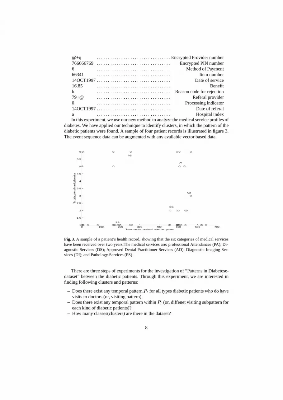
diabetes. We have applied our technique to identify clusters, in which the pattern of thediabetic patients were found. A sample of four patient records is illustrated in figure 3.The event sequence data can be augmented with any available vector based data.

0 100 200 300 400 500 600 7001

1.5

2

2.5

3

3.5

4

4.5

5

5.5

6

Six c

atego

ries o

f med

ical s

ervic

e

Treatments received over two years

DS

AD

DI

PS

PA

Fig. 3. A sample of a patient’s health record, showing that the six categories of medical serviceshave been received over two years.The medical services are: professional Attendances (PA); Di-agnostic Services (DS); Approved Dental Practitioner Services (AD); Diagnostic Imaging Ser-vices (DI); and Pathology Services (PS).

There are three steps of experiments for the investigation of “Patterns in Diabetese-dataset” between the diabetic patients. Through this experiment, we are interested infinding following clusters and patterns:

– Does there exist any temporal patternPt for all types diabetic patients who do havevisits to doctors (or, visiting pattern).

– Does there exist any temporal pattern withinPt (or, diffenet visiting subpattern foreach kind of diabetic patients)?

– How many classes(clusters) are there in the dataset?

8

– What kinds of patterns (models) are there for each class?– What kind of a relationship exists between classes?

3.1 On structural pattern searching

We are investigating the data structural base to test naturalness of the similarity andperiodicity on Structural Base distribution. We consider 6 states in the state-space ofstructural distribution:S= fs1; s2; s3; s4; s5; s6g.

For searching structural (or, qualitative) patterns, we use limit theorem on transitionprobability matrix�k for each patient. We found there are exist three clusters:

– In cluster one, visiting temporal pattern is a stationary process. The meaning is thatall the patients see their doctors regularly for consulatations and treatments,

– In cluster two, visiting temporal pattern is combinatoral Poisson process. This meanis that all the patients temporal behaviour(e.g., time distance between successivepair of two consultations or, between successive pair of two treatments) not sym-metricaround their mean, but much extending to the right(e.g., patient has a fewernumber of consulatations than the number of medical-treatments). It is also tell us,the patient in this group is a new diab-patient, or the patient has other problemsother than diabetes, so they need more medical treatments.

– In cluster three, all the patients have a larger number of consulatations than thenumber of medical-treatments, for example, they may get other sicknesses such ascold very easily.

For example, in Figure 4, figures in each row from bottom to top is cluster one,cluster two and cluster three. “CC” means consultation to consultation, “CT” meansconsultation to treatments and so on. Thex-axis represents the transition probabilitybefore using the limit theorem and they-axis represents transition probability after us-ing the limit theorem. This explains two facts: (1) there exists some sub-group whichcorresponds to patterns on the same condition in the group, and (2) there exist par-tial similar patterns between clusters. In summary, some results for the structural base

0 0.1 0.2 0.3 0.4 0.5 0.6 0.7 0.8 0.9 10

0.5

1

0 0.1 0.2 0.3 0.4 0.5 0.6 0.7 0.8 0.9 10

0.5

1

0 0.1 0.2 0.3 0.4 0.5 0.6 0.7 0.80

0.5

1

Z CT to TC

I CT to TC

C CT to TC

0 0.1 0.2 0.3 0.4 0.5 0.6 0.7 0.8 0.9 10

0.5

1

0 0.1 0.2 0.3 0.4 0.5 0.6 0.7 0.8 0.9 10

0.5

1

0 0.1 0.2 0.3 0.4 0.5 0.6 0.7 0.8 0.9 10.2

0.4

0.6

0.8

1

Z CC to TT

I CC to TT

C CC to TT

Fig. 4. plot of the transition probability between consulatation state and medical-treatment statein all states.

9

experiments are as follows:

– more than half percent of diabetes-patients have other major medical problems:patients have other major medical problems based on their type of diabetes. Thereexist similar patterns between major medical problems in structure of each of threeclusters.

– less than half percent of diabetes-patients get “seasonal health problems” very eas-ily: there also exist some similar patterns between each subgroup in structure (itmay be related to their age).

– only 0.05 percent of normal patients are diab-patients: this means they do not haveother major medical problems and they do not easily get “seasonal health prob-lems”.

3.2 On value-point pattern searching

We now illustrate our new method on the value-point sequence for searching patterns.Recall data model and data vector sequence

Y = m(V) + �(V)" =

pXj=0

�j(v� v0)j + #p; let Vj = fv1j ; v2j ; � � � ; vNjg;

each vectorVj are time vector variable, e.g.,vkj (k =1, 2, : : :, N ) is the time lengthbetween the statesk andsj has occurred.

In the light of our structural base experiments, we have found that there exists a lin-ear regression function between categories8 in each of the three clusters. For example,if let Ck

i (t) be a time series distribution function for one categoryk, and its responsevariable is time distance between successive two time point(e.g., a patient visits doctorand use items in same category) then the time seriesV k

i;j(t) which difference betweentwo linear regrassion functions at timet valuesV k

i;j(t) = Cki (t)�Ck

j (t) is an approxi-mate distribution function.

For example, in Figure 5, thex-axis represents how many items have been used, they-axis represents the accumulated occurences of each item, and thez-axis represents sixcategories.

Some results for the value-point of experiments are as follows9:

– There does exist some periodic patterns in the same cluster but with different cate-gory.

– There exist some similarity patterns in each cluster, but between different cate-gories.

– There exist some similarity patterns between the same category from each cluster.

8 There are six categories in Australia Medicare Benefits Schedule Book9 We classify repeating patterns based on a distance classification technique.

10

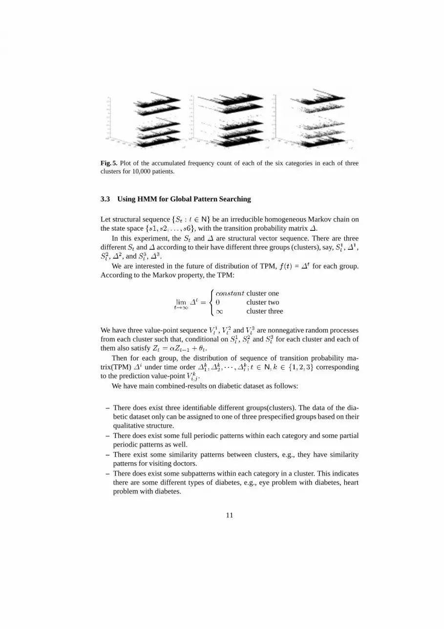
Fig. 5. Plot of the accumulated frequency count of each of the six categories in each of threeclusters for 10,000 patients.

3.3 Using HMM for Global Pattern Searching

Let structural sequencefSt : t 2 Ng be an irreducible homogeneous Markov chain onthe state spacefs1; s2; : : : ; s6g, with the transition probability matrix�.

In this experiment, theSt and� are structural vector sequence. There are threedifferentSt and� according to their have different three groups (clusters), say,S1t ,�1,S2t , �2, andS3t , �3.

We are interested in the future of distribution of TPM,f(t) = �t for each group.According to the Markov property, the TPM:

limt!1

�t =

8<:constant cluster one0 cluster two1 cluster three

We have three value-point sequenceV 1t , V 2

t andV 3t are nonnegative random processes

from each cluster such that, conditional onS1t , S2t andS3t for each cluster and each ofthem also satisfyZt = �Zt�1 + �t:

Then for each group, the distribution of sequence of transition probability ma-trix(TPM) �i under time order�k

1 ; �k2 ; � � � ; �

kt ; t 2 N; k 2 f1; 2; 3g corresponding

to the prediction value-pointV ki;j :

We have main combined-results on diabetic dataset as follows:

– There does exist three identifiable different groups(clusters). The data of the dia-betic dataset only can be assigned to one of three prespecified groups based on theirqualitative structure.

– There does exist some full periodic patterns within each category and some partialperiodic patterns as well.

– There exist some similarity patterns between clusters, e.g., they have similaritypatterns for visiting doctors.

– There does exist some subpatterns within each category in a cluster. This indicatesthere are some different types of diabetes, e.g., eye problem with diabetes, heartproblem with diabetes.

11

4 Related Work

In recent years various studies have considered temporal datasets for searching differentkinds of and/or different levels of patterns. For example, many researchers use statisti-cal techniques such as Metric-distance based techniques, Model-based techniques, or acombination of techniques (e.g, [10]) to search for different pattern problems such asin periodic patterns searching (e.g., [4]) and similarity pattern searching (e.g., [3]).

Our work is different from these works. First, we use a statistical language to per-form all the search work. Second, we divide the data sequence or, data vector sequence,into two groups: one is the structural base group and the other is the pure value basedgroup. In group one our techniques are similar to Agrawal’s work but we only considerthree state changes (i.e., up (value increases), down (value decreases) and same (nochange)) whereas Agarwal considers eight state changes (i.e., up (slightly increasingvalue), Up (highly increasing value), down (slightly increasing value) and so on). In thisgroup, we also use distance measuring functions on structural based sequences whichis similar to [8]. In group two we apply statistical techniques such as local polynomialmodelling to deal with pure data which is similar to [2]. Finally, our work combinessignificant information of two groups to get global information which is behind thedataset.

5 Concluding Remarks

This paper has presented a new approach of hidden Markov models to mining temporalpatterns. The rough decision for pattern discovery comes from the structural level that isa collection of certain predefined similarity patterns. The clusters of similarity patternsare computed in this level on state-space by the choice of certain states. The point-value patterns are decided in the second level and the similarity and periodicity of aDTS are extracted. In the final level, we combine structural and value-point patternsearching into the HMM model to obtain a global pattern picture and understand thepatterns in a dataset better. Another approach to find similar and periodic patterns havebeen reported in [5–7]; there the model used is based on hidden periodicity analysis.However, we have found that using different models at different levels produces betterresults.

The method guarantees finding different patterns if they exist with structural andvalued probability distribution of a real-dataset. The results of preliminary experimentshave been shown to be promising and we are currently applying the method to othertypes of large realistic medical data sets.

References

1. C. Bettini. Mining temportal relationships with multiple granularities in time sequences.IEEE Transactions on Data & Knowledge Engineering, 1998.

2. G. Das, K. Lin, H. Mannila, G.Renganathan, and P. Smyth. Rule discovery from time series.In Proceedings of the international conference on KDD and Data Mining(KDD-98), 1998.

12

3. G.Das, D.Gunopulos, and H. Mannila. Finding similar time seies. InPrinciples of Knowl-edge Discovery and Data Mining ’97, 1997.

4. Cen Li and Gautam Biswas. Temporal pattern generation using hidden markov model basedunsuperised classifcation. InProc. of IDA-99, pages 245–256, 1999.

5. Wei Q. Lin and Mehmet A.Orgun. Applied hidden periodicity analysis for mining discrete-valued time series. InProceedings of ISLIP-99, pages 56–68, Demokritos Institute, Athens,Greece, 1999.

6. Wei Q. Lin and Mehmet A.Orgun. Temporal data mining using hidden periodicity analysis.In Proceedings of ISMIS2000, University of North Carolina, USA, 2000.

7. Wei Q. Lin, Mehmet A.Orgun, and Graham Williams. Temporal data mining usingmultilevel-local polynomial models. InProceedings of IDEAL2000, The Chinese Univer-sity of Hongkong, Hong Kong, 2000.

8. S.Jajodia andS.Sripada O.Etzion, editor.Temporal databases: Research and Practice.Springer-Verlag,LNCS1399, 1998.

9. P.Baldi and S. Brunak.Bioinformatics & The Machine Learning Approach. The MIT Press,1999.

10. Z.Huang. Clustering large data set with mixed numeric and categorical values. In1st Pacific-Asia Conference on Knowledge Discovery and Data Mining, 1997.

13