Proceedings of Machine Learning Research 126:1–21, 2020 Machine Learning for Healthcare

Personalized Input-Output Hidden Markov Models forDisease Progression Modeling

Kristen A. Severson kristen.severson@ibm.com†

Center for Computational HealthIBM ResearchCambridge, MA USA

Lana M. Chahine lanachahine@pitt.eduDepartment of NeurologyUniversity of PittsburghPittsburgh, PA USA

Luba Smolensky lsmolenky@michaeljfox.orgMichael J. Fox FoundationNew York, NY USA

Kenney Ng kenney.ng@us.ibm.com

Jianying Hu jyhu@us.ibm.com

Soumya Ghosh ghoshso@us.ibm.com†

Center for Computational Health

IBM Research

Yorktown Heights, NY and Cambridge, MA USA†Corresponding authors

Abstract

Disease progression models are important computational tools in healthcare and are usedfor tasks such as improving disease understanding, informing drug discovery, and aiding inpatient management. Although many algorithms for time series modeling exist, healthcareapplications face particular challenges such as small datasets, medication effects, diseaseheterogeneity, and a desire for personalized predictions. In this work, we present a diseaseprogression model that addresses these needs by proposing a probabilistic time-series modelthat captures individualized disease states, personalized medication effects, disease-statemedication effects, or any combination thereof. The model builds on the framework of aninput-output hidden Markov model where the parameters are learned using a structuredvariational approximation. To demonstrate the utility of the algorithm, we apply it toboth synthetic and real-world datasets. In the synthetic case, we demonstrate the benefitsafforded by the proposed model as compared to standard techniques. In the real-worldcases, we use two Parkinson’s disease datasets to show improved predictive performancewhen ground truth is available and clinically relevant insights that are not revealed viaclassic Markov models when ground truth is not available.

1. Introduction

Disease progression models are an important tool for understanding the characteristics andprogression trends of a wide variety of diseases. Applications of disease progression models

c© 2020 K.A. Severson, L.M. Chahine, L. Smolensky, K. Ng, J. Hu & S. Ghosh.

PIOHMM for DPM

include drug development (Mould, 2012), patient care management (Tangri et al., 2011),and better understanding disease mechanisms (Lorenzi et al., 2019). Prediction tasks,including disease progression as well as the occurrence of specific outcomes, is a criticalelement of all of the latter. Disease progression modeling faces challenges that lead tospecific algorithmic requirements. Here, we highlight and discuss four specific challenges:small datasets, a modeling goal of uncovering states, confounding of symptom presentationdue to medication effects, and a desire to personalize prediction. We discuss each of thesein more detail below.

• Small datasets. Often, the amount of data available for modeling tasks is limiteddue to various causes such as the cost of acquiring the data, the enrollment burdenon patients, study attrition, and data privacy issues. These small datasets motivatethe incorporation of prior knowledge into the model structure.

• Uncovering disease states. In many scenarios, disease progression models aimto both learn a quantitative model of future patient state along with salient diseasestates. Although some diseases have clearly definable pathologic stages, such as incancer, many diseases do not have this characterization and discovering such stagesis an important research goal. These states can be used for downstream tasks such ascohort generation and improved disease understanding.

• Confounding due to medication effects. The datasets used for disease progres-sion modeling are often complicated by medication effects, particularly in settingsleveraging observational data. Medications may alter the symptoms of the patient,the underlying disease state, or both.

• Personalized predictions. For heterogeneous diseases, there are many factors whichmay impact a particular patient’s disease progression, necessitating the modeling ofpersonalized trajectories.

Disease progression models that address the aforementioned critical factors are partic-ularly relevant for chronic diseases which are heterogeneous in both their manifestationsand progression. In this setting, simple predictors of future disease state are ineffective.Parkinson’s disease (PD) is a useful case study for understanding the importance of dis-ease progression modeling. PD is a chronic progressive neurodegenerative disorder withheterogeneous symptoms that may affect both motor and non-motor function. Two clin-ical subtypes of PD have been proposed (Zetusky et al., 1985), however the stability andprogression of these subtypes is not well understood (Simuni et al., 2016). There are nomedications that cure PD, however medications that improve quality of life by address-ing common symptoms are available. The degree of response to medications, duration ofresponse, and tolerance of medications vary from patient to patient. Disease progressionmodels for PD would enable all of the benefits discussed above: improved disease under-standing, patient care management, and drug development. PD is characteristic of manychronic conditions (e.g. Alzheimer’s disease, diabetes, ALS) where no disease-modifyingtherapeutics are available and is used to demonstrate our proposed approach.

The goal of the work is to model disease progression while taking medication effects andpersonalized disease trajectories into account. Motivated by PD and many other conditions

2

PIOHMM for DPM

for which there are currently no disease-modifying therapeutics, we focus on the scenariowhere medication does not alter the underlying disease but does alter the observations.

Generalizable Insights about Machine Learning in the Context of Healthcare

In this work, we propose a probabilistic disease progression modeling framework to addressthe needs discussed above. Our models have the ability to account for personalized stateand medication effects while learning disease states. This enables us to model heterogeneityin the disease population, a common characteristic of complex diseases. By carefully choos-ing the model structure, the parameters of these models can be learned without access tolarge datasets. Probabilistic models are particularly useful for disease progression modelingwhen one of the goals is to learn underlying disease states. Probabilistic models also havethe ability to incorporate prior information, provide natural handling for missing data, andenable parameter uncertainty calculations. Because of these advantages, our research fo-cuses on adapting probabilistic time series models for disease progression modeling. We relyon black-box variational inference and employ variational approximations that retain themodel structure to perform accurate learning and inference. We demonstrate our approachon a synthetic dataset as well as two Parkinson’s disease datasets.

2. A personalized and medication aware disease progression model

Our proposed model builds on the hidden Markov model (HMM). A hidden Markov modeldescribes sequential data through a series of transitions between latent states, with eachstate describing distinct characteristics of the observed data instances. An HMM has twoprimary components: (1) the transition model which describes the evolution of states overtime and (2) the observation model which describes the manifestation of the state in ob-served space. Here, the latent states are denoted by z, with zi corresponding to patienti’s full trajectory and zi,t corresponding to an element in that trajectory at time t. Anal-ogously, observations are denoted by x and medications are denoted by d. See Table 1 foradditional details of the mathematical notation.

In our work, we use a standard transition model,

zi,1 ∼ Cat(π), zi,t | zi,t−1 = j ∼ Cat(Aj), (1)

where π ∈ RK+ ,∑K

k=1 πk = 1 and A ∈ RK×K+ ,∑K

k=1Ajk = 1. Cat(·) indicates a categoricaldistribution. An HMM with a Gaussian observation model is specified as xi,t | zi,t =k ∼ N (µk,Σk), where N (µ,Σ) represents a multivariate Gaussian distribution with meanµ ∈ RD and covariance Σ ∈ RD×D. Below, we present observation models to account forsystematic personalized and medication effects.

Medication-aware HMMs Assuming that medication information (di,t) is available ateach time step along with the observed data xi,t, the proposed observation model is

xi,t | zi,t = k, di,t ∼ N (µk + vkdi,t,Σk), (2)

where vk ∈ RD×M where M is the number of medications. The additive structure modelsstate-specific deviations in the observed data from the disease state based on the presence

3

PIOHMM for DPM

of medication. The exact details of the implementation will depend on the expected impactof the drug. For instance, if the medication effect is not a function of the medication dose,di,t can be binary. Alternatively, the effect is scaled based on the dose. If the effect ofmedication does not vary along the disease trajectory, the model can be altered such thatvk = v ∀k.

For complex diseases, we expect medication responses to vary both among patientsand also within the same patient along with the severity of the disease. We can modifyEquation 2 to account for such effects by introducing state-specific effects for each patient,xi,t | zi,t = k, di,t ∼ N (µk + vi,kdi,t,Σk). However, the large number of parameters vi,k,makes learning challenging in such a model. Indeed, we expect to observe most patients inonly a subset of all possible states, and inferences of vi,k based on such data are likely to beunreliable. To circumvent this problem, we propose an alternate model where we factorizethe medication effects into state-specific and patient-specific components,

xi,t | zi,t = k, di,t ∼ N (µk + (vk +mi)di,t,Σk). (3)

The state specific coefficients vk are shared across observations assigned to state k, whilemi is shared across all observations from patient i. Such a factorization allows us to sharestatistical strength both between observations assigned to a common state and observationsbelonging to the same patient, thus providing more reliable inferences of personalized statespecific medication effects.

Personalized HMMs To allow patients to deviate from the population at large, not asa function of medication, we introduce patient specific latent variables ri ∈ RD to modifythe mean response of patient i,

xi,t | zi,t = k ∼ N (µk + ri,Σk). (4)

This enables personalization in how states might manifest in an individual.It is natural to consider a more general variant that combines Equations 2 and 4 to

account for both medication independent heterogeneity in the population as well as person-alized medication effects,

xi,t | zi,t = k, di,t ∼ N (µk + ri + (vk +mi)di,t,Σk). (5)

For ease of exposition, we frame the following discussion and the description of our learningalgorithm in the context of this model (Equation 5) which subsumes the medication-awareand personalized models. Learning and inference in the models described via Equations 2and 4 are analogous.

Priors We place Gaussian priors on the personalized effects (mi and ri) and the state-specific medication effects (vk)

mi ∼ N (0, σ2mID), ri ∼ N (0, σ2rID), vk ∼ N (0, σ2vID). (6)

By employing zero mean Gaussian priors with appropriately chosen variances σ2m and σ2r weencode our prior belief that while heterogeneity among patients and between states exists,the scale of this heterogeneity is small and the personalized effects do not deviate too far

4

PIOHMM for DPM

Figure 1: The graph for the proposed model: z are the latent states, x are the observedvariables, d are observed medications, r are the personalized state effects, andm are the personalized medication effects. φk and vk are parameters of theobservation model. A and π are parameters of the transition model.

N Number of patients, indexed i ∈ {1, . . . , N} λ Variational parametersT Number of time points, indexed t ∈ {1, . . . , T} θ Model parametersD Dimensionality of the observations per time point π Initial state distributionK Number of latent states A State transition distributionsx Observed clinical data vk State medication effectsz Latent states φk State parameters includingd Observed medication data µk, state means, and Σk,m Personalized medication effects state covariancer Personalized state effects

Table 1: Summary of notation used throughout the paper.

from the overall population. The prior over vk regularizes its value and encourages themodel to use the personalized effects mi to explain the observed data.

Equations 1, 5, and 6 completely describe our model. The model parameters are θ ={A, π, µk,Σk, vk, σ

2m, σ

2r} and the random variables are {x, z,m, r}. The resulting graphical

model is shown in Figure 1. We refer to it as the personalized input-output hidden Markovmodel (PIOHMM) owing to its similarity to the input output HMM (IOHMM) (Bengio andFrasconi, 1995)1.

1. To arrive at IOHMM from PIOHMM, set ri = 0, and mi = 0.

5

PIOHMM for DPM

3. Learning Algorithm

We use variational methods to learn the proposed model. We approximate the poste-rior distributions over the local latent variables ({zi,mi, ri}Ni=1) with tractable variationalapproximations and rely on point estimates for the global parameters (θ). Our choice ofperforming point inference for global parameters, those shared by more than one individual,while inferring full distributions for local random variables is motivated by the expectationthat local variables which are only informed by a individual’s data would exhibit higher un-certainty. We employ a structured variational approximation that retains the dependencebetween zi and mi, ri, and also, crucially, the temporal structure within zi,

q(z,m, r | x, λ) =

N∏i=1

q(mi | λmi)q(ri | λri)q(zi | xi,mi, ri),

=N∏i=1

q(mi | λmi)q(ri | λri)q(zi,1 | xi,mi, ri)T∏t=2

q(zi,t | zi,t−1, xi,mi, ri),

(7)

where λ are the variational free parameters. We use Gaussians with full covariances toparameterize the variational distributions, q(mi | λmi) , N (mi | µmi , LmiL

Tmi

) and q(ri |λri) , N (ri | µri , LriLT

ri), L· are lower triangular matrice, and use categorical distributionsfor zi,t.

We minimize the Kullback-Leibler divergence between the variational approximation andthe true posterior as well as learn the model parameters, θ by maximizing the correspondingevidence lower bound (ELBO),

L(θ, λ) = Eq(z,m,r|x,λ)[ln p(x, z,m, r | θ)] + H[q(z,m, r | x, λ)], (8)

where H[q(·)] = −Eq[ln q(·)] is the entropy and the log joint distribution is (see Figure 1),

ln p(x, z,m, r | θ) =

N∑i=1

ln p(mi | σ2m) +

N∑i=1

ln p(ri | σ2r ) +

N∑i=1

ln p(zi,1 | π)+

N∑i=1

T∑t=2

ln p(zi,t | zi,t−1, Azi,t−1) +

N∑i=1

T∑t=1

ln p(xi,t | zi,t, di,t,mi, ri, vzi,t , φzi,t)

(9)

and φzi,t = {µzi,t ,Σzi,t}.We maximize the ELBO via coordinate ascent alternating between updates to varia-

tional parameters λ and model parameters θ. Our structured variational approximation,Equation 7, renders expectations required to compute the ELBO intractable. We deal withthis issue by using Monte Carlo approximations of the offending expectations and relying onpathwise gradient estimators to differentiate through the sampling process. In particular,we approximate,

Eq(zi,mi,ri|xi,λ)[ln p(xi | zi,mi, ri, θ)] ≈1

S

S∑s=1

Eq(zi|xi,mi=msi ,ri=r

si )

[ln p(xi | zi,mi = msi , ri = rsi , θ)],

(10)

6

PIOHMM for DPM

where msi = Lmiε

smi

+ µmi , rsi = Lriε

sri + µri and εsmi

∼ N (0, I) and εsri ∼ N (0, I). Cru-cially, we do not need to use a Monte Carlo approximation for evaluating the conditionalexpectation in Equation 10. Instead we note that we can exactly compute the conditionaldistribution q(zi | xi,mi, ri), using the forward-backward algorithm (Baum, 1972; Rabiner,1989), a dynamic programming algorithm widely used to learn hidden Markov models, andefficiently compute the conditional expectation by exploiting the Markovian dependenciesin the model. These operations are identical to those needed by standard expectation max-imization training of HMMs (see appendix for additional details). Given the Monte Carloexpectation we take a stochastic gradient ascent step to update the variational parametersλ (Kingma and Ba, 2015). Conditioned on λ, maximizing the ELBO with respect to θcan be done via fixed point updates (see appendix for details). The overall algorithm issummarized in Algorithm 1.

Algorithm 1: Training procedure of PIOHMM

Input: Model p(D; θ), variational approximations q(mi | λm), q(ri | λr)Output: Optimized model and variational parameters, θ, λInitialize parameters {π,A, vk, µk,Σk, σ

2m, σ

2r} ∀k ∈ K;

Initialize variational parameters {µmi , Lmi , µri , Lri } ∀i ∈ Nfor 1, . . . , Niter do

Sample εsmi∼ N (0, I), εsri ∼ N (0, I) ∀i ∈ N ;

Set msi = Lmiε

smi

+ µmi , rsi = Lriε

sri + µri ∀i ∈ N ;

Use forward-backward algorithm to calculate q(zi | xi,mi, ri) ∀i ∈ N ;Update λn+1 ← ADAM(λn,L(λ, θ));Use fixed point equations to update θ.

end

4. Related Work

Markov models are not the only class of models that have been considered for disease pro-gression modeling. Several authors have considered Gaussian process (GP) models (Lorenziet al., 2019; Schulam and Saria, 2015; Futoma et al., 2016). GP models are convenientin that they do not require samples to be observed at a fixed rate, are non-parametricprobabilistic models, and have been shown to be capable of personalization (Schulam andSaria, 2015). However, GP based models are typically unable to discover discrete states ofa disease, one of the goals of our work. Similarly, deep learning methods have also beenproposed for disease progression modeling (Che et al., 2018; Eulenberg et al., 2017; Phamet al., 2017). While these approaches are able to predict future clinical features, they alsodo not discover discrete states of progression of a disease. Moreover, they typically needlarge datasets often requiring tens of thousands of patients records, as is the case in thecited works.

HMMs are well suited to disease progression modeling, particularly when there is aninterest in discovering stages of progression. Several studies have leveraged HMMs andvariations for disease progression modeling in the past, e.g. Jackson et al. (2003); Sukkaret al. (2012); Guihenneuc-Jouyaux et al. (2000). Wang et al. proposed continuous time

7

PIOHMM for DPM

HMMs to model the progression of chronic disease. Sun et al. leveraged this approachto develop an integrated Huntington’s disease progression model. However none of theseprevious approaches model system inputs, such as medication, or account for heterogene-ity in symptoms between patients in a cohort. Bengio and Frasconi proposed input-outputHMMs (IOHMM) as a way to model an observed control signal for a system. In an IOHMM,the inputs influence the observed and/or latent variables. Our work extends IOHMMs toaccount for medication independent patient heterogeneity while leveraging their ability tomodel external inputs to account for non disease modifying medications. Altman (2007)worked on extending HMM models to account for personalized effects and external inputs.However, unlike us, they relied on Monte Carlo expectation maximization to learn thesemodels, which typically requires running a MCMC sampler within each expectation stepand is difficult to scale to both high dimensional data and number of patients. In con-trast, our stochastic gradient variational inference approach easily scales along both thesedimensions. Finally, recent work by Alaa and van der Schaar (2019) proposes to relax thefirst order Markovian assumption made by typical HMM based disease progression modelsand personalize progression dynamics across patients. Our contributions are orthogonal, wepersonalize HMM observation models rather than dynamics. A combination of these twoadvances comprises an interesting future research direction.

5. Results

To demonstrate the algorithm, we apply it to three test cases: a synthetic dataset, a real-world dataset of sensor data from Parkinson’s patients with labeling and a real-world datasetof clinical data from Parkinson’s patients without labeling. In all three cases we demonstratethat the proposed model outperforms other HMM variants.

5.1. Synthetic Data

We generate data by considering the following model. First, generate a sequence of latentstates governed by the distributions, zi,1 ∼ Cat(π), zi,t | zi,t−1 = j ∼ Cat(Aj). Thengenerate observations using, xi,t | zi,t = k ∼ N (µk,Σk). For each sample i, a personalizedoffset is sampled, ri ∼ Unif[−b, b]. Lastly, structured noise is added to the observationxi | xi, ri ∼ N (xi+ri,ΣT ), where ΣT is specified via a squared exponential kernel, κ(t, t′) =

σ2 exp −(t−t′)2

2l2. Note that this model is not exactly the same as the proposed model and

that when b = 0, the observed data is a noisy observation of an HMM with correlated noise.To simplify the visualization of the results, the dimensionality of the observed data is

fixed to one and the number of latent states is two. 100 samples of length 20 are generatedas described above and experiments are performed for b = 0, 1, 5. The true state means are0 and 2 and the state variance is 0.1. The results are shown in Figure 2. The experimentdemonstrates how the personalized HMM performs no worse than the HMM when person-alized effects are not present, and is much better at recovering the state dynamics whenpersonalized effects are present. Because the HMMs is not able to capture personalized dif-ferences, the model compensates by inflating the variance of the states and therefore doesa poor job of capturing state dynamics.

8

PIOHMM for DPM

Figure 2: Results for simulated data. The three rows correspond to different distributionsof ri ∼ Unif[−b, b] and the four leftmost columns correspond to samples. Therightmost column plots the inferred ri vs. the sample index. When there are nopersonalized effects, the personalized and classic HMMs perform approximatelythe same and the personalized model learns personalized parameters close to zero,as shown in the last column. When a personalized offset does exist, the classicHMM incorrectly assigns states and compensates for the personalization withlarge variances, as shown in rows two and three. When personalized effects arelarger than state effects, a prior to regularize the state effects is appropriate. Ananalysis of the inferred ri enables the practitioner to identify samples with largedeviations, which may be of special interest.

5.2. Application: Parkinson’s Disease

To demonstrate the approach on a real-world dataset, we apply the method to two datasetsof Parkinson’s disease patients. As noted in the introduction, Parkinson’s disease (PD) isa chronic neurodegenerative disorder (Jankovic, 2008). PD is characterized by a variety ofmotor and non-motor features and a definitive diagnostic test is not available. Typicallydiagnosis depends on the presence of specific clinical features, namely rest tremor, rigid-ity, bradykinesia, and/or postural instability (Jankovic, 2008; Postuma et al., 2015). Theheterogeneity of PD symptoms and progression is well-documented but poorly understood(Zetusky et al., 1985; Kehagia et al., 2010). These features make the disease a good fit forour method to learn a clinical representation of disease states as well as how these statesevolve in time.

In our first study, we demonstrate the algorithm for the problem of identifying freezingof gait. Freezing of gait is a severe complication of PD resulting in falling, reduced mo-bility, and increased disability. Identifying objective ways to accurately detect it thus hasimportant clinical implications. In this setting, we have access to ground truth labels from

9

PIOHMM for DPM

clinical annotators and the relevant states are known: standing, walking, and freezing. Inthe second study, we apply the algorithm to the more general problem of discovering PDdisease states. We describe the resulting states in the context of the current PD literature.

5.2.1. Case Study with Labeled States

Data Description As noted above, the goal of this study was to identify when a patientis experiencing freezing of gait. The study uses the Daphnet Freezing of Gait Dataset, abenchmark dataset which contains information from wearable acceleration sensors (Bachlinet al., 2010). Ten patients are included in the dataset and each has 9 measurements:horizontal forward, horizontal lateral and vertical acceleration from ankle, thigh and trunksensors. We follow the data processing procedure presented in Bachlin et al. (2010) andtransform overlapping time windows into the freeze index for each patient and sensor. Twopatients have no freezing of gait events and are removed from our study. The time trajectoryof each patient is then divided into training and testing sequentially with the first 400 timesteps (200 seconds) used for training and the subsequent 400 time steps used for testing.

Model Description For this application, we choose the observation model

xi,t | zi,t = k ∼ N (µk + ribk,Σk) (11)

which has personalized state effects. This is motivated by the original study which notesthat their detection model has variable performance due to the different walking styles ofthe patient. There are three pre-defined states: standing, walking, and freezing of gait.We do not expect personalized differences in standing, therefore we introduce a variableb = [0, 1, 1], such that ri has no effect for one of the states. Note that beyond specifying b,no special care is taken in initializing the model during training. A second model using aclassic hidden Markov model is also trained for comparison. This model has the observationmodel

xi,t | zi,t = k ∼ N (µk,Σk). (12)

Results The two models are compared using several metrics. The test log likelihoodsare -238181 and -238660 for the personalized and standard models, respectively, implyingthe personalized model is better at describing the data. Figure 3 shows an example of thefreeze index for one sensor and the corresponding prediction for patient 9 along with modelmetrics. The receiver operating curve is calculated for each model using the belief state ofthe freezing state

p(zit = FOG | xi,1:t). (13)

The AUCs are 0.725 and 0.705 for the personalized and standard model, respectively, indi-cating slightly better performance for the personalized model.

Qualitatively, the inferred personalized state effects, ri, can be used to identify outlierpatients, who may be of interest. Here, the largest ri corresponds to the patient with thelargest Hoehn and Yahr score, a measure of PD severity not used in model training.

5.2.2. Case Study without Labeled States

Data Description For this study, we use the Parkinson Progression Marker Initiative(PPMI) dataset (Marek et al., 2011). PPMI is an observational, longitudinal, multi-center

10

PIOHMM for DPM

Figure 3: Results from the case study with labeled states. Moving from left to right, theupper plot shows the freeze index for the ankle sensor acceleration in the verticaldirection. The lower plot shows the state prediction (dotted line) compared toground truth (solid line). Note that the ground truth labels do not differentiatedifferent tasks and only have information for freezing of gait (FOG) or no freezingof gait. The right plot shows the receiver operator curve for the test data usingthe personalized and standard hidden Markov models using the belief state forthe freezing state. The AUCs are 0.725 and 0.705, respectively.

study that enrolled 423 PD patients. PPMI collects clinical, imaging, and biospecimen sam-ples. In this analysis, we focus on the clinical assessments, specifically those measured viathe Movement Disorder Society Unified Parkinson’s Disease Rating Scale (MDS-UPDRS)(Goetz et al., 2008). The MDS-UPDRS is a four part assessment that contains a combina-tion of patient reported- and physician-assessed measures. The four parts are: (I) non-motorexperiences of daily living, (II) motor experiences of daily living, (III) motor examination,and (IV) motor complications. Each item on the scale is rated from 0 (normal) to 4 (severe).For our study, we do not use part IV therefore the observed data has 59 dimensions.

Levodopa is the primary medication used to treat Parkinson’s disease and is thoughtto have no disease-modifying effect (Verschuur et al., 2019). Levodopa is a dopaminergicmedication and is primarily used to treat motor symptoms. Levodopa may be administeredin concert with other medications such as a dopamine agonist, monoamine oxidase type Binhibitor, or a catechol-O-methyl transferase inhibitor. In order to model the combination ofthese drugs in a consistent manner, the levodopa equivalent daily dose (LEDD) (Tomlinsonet al., 2010) has been developed. LEDD information is provided in PPMI and used to modelmedication effects in our study. Per the PPMI protocol, PD patients must not have startedmedications at time of enrollment and initiate different medications at varying times overthe study, depending on specific patient characteristics. The dose as well as the responsechanges over time. Medication effects are captured to some degree by motor examinationoccurring prior to intake of levodopa or dopamine agonists, and repeated again 1-4 hoursafter medication are taken. This process is referred to as ‘on-off’ testing.

11

PIOHMM for DPM

Figure 4: Scatter plots showing the per sample test log-likelihood (N=83) for the threedifferent Markov models. The number on the plot indicates the number of samplesthat are above the diagonal line. These results show that the PIOHMM improvesupon both the IOHMM and HMM in terms of test log likelihood.

Model Description Based on domain understanding of Parkinson’s disease, we choosethe observation model

xi,t | zi,t = k, di,t ∼ N (µk + (vk +mi)di,t,Σk). (14)

This model captures our prior beliefs that there are several unknown disease states whoseobservations are impacted by medication use. We expect that the impact of medicationis a function of both the individual and the disease state. The transition matrix, A isconstrained to be upper triangular to enforce progressive disease states.

A full distribution of the number of visits per patient is available in the appendix; onaverage, the patients have observations through 21 visits and a total of 12 observed visits.This discrepancy is a result of the PPMI protocol, which increases the time between visitsas the time since enrollment increases. Because the protocol establishes a visit scheduleprior to patient enrollment, a missing at random assumption is reasonable. We note that itis possible that patients deviate from their schedule based on their disease status but didnot find evidence to that effect and proceeded with an assumption of data that is missingat random (see appendix for more detail). The time step is fixed to three months and anymissing values are marginalized. The dataset is divided into training and testing with 333patients used for training and 83 patients used for testing. Patients with only one observa-tion were excluded (N=7). To compare with the proposed PIOHMM, standard HMM andIOHMM models are also developed. For all models, we use a 5-fold cross validation strategyon the training data to select the number of states.

Results Figure 4 plots the test log-likelihood per patient for the three models. ThePIOHMM outperforms the other models, suggesting that the PIOHMM is a better modelfor the data.

By modeling personalized-medication and state-medication effects, we hope to recoverrelevant clinical latent states. To characterize the states, we perform a post-hoc analysis,focusing on the primary clinical symptoms used for diagnosis: tremor, bradykinesia, rigidity

12

PIOHMM for DPM

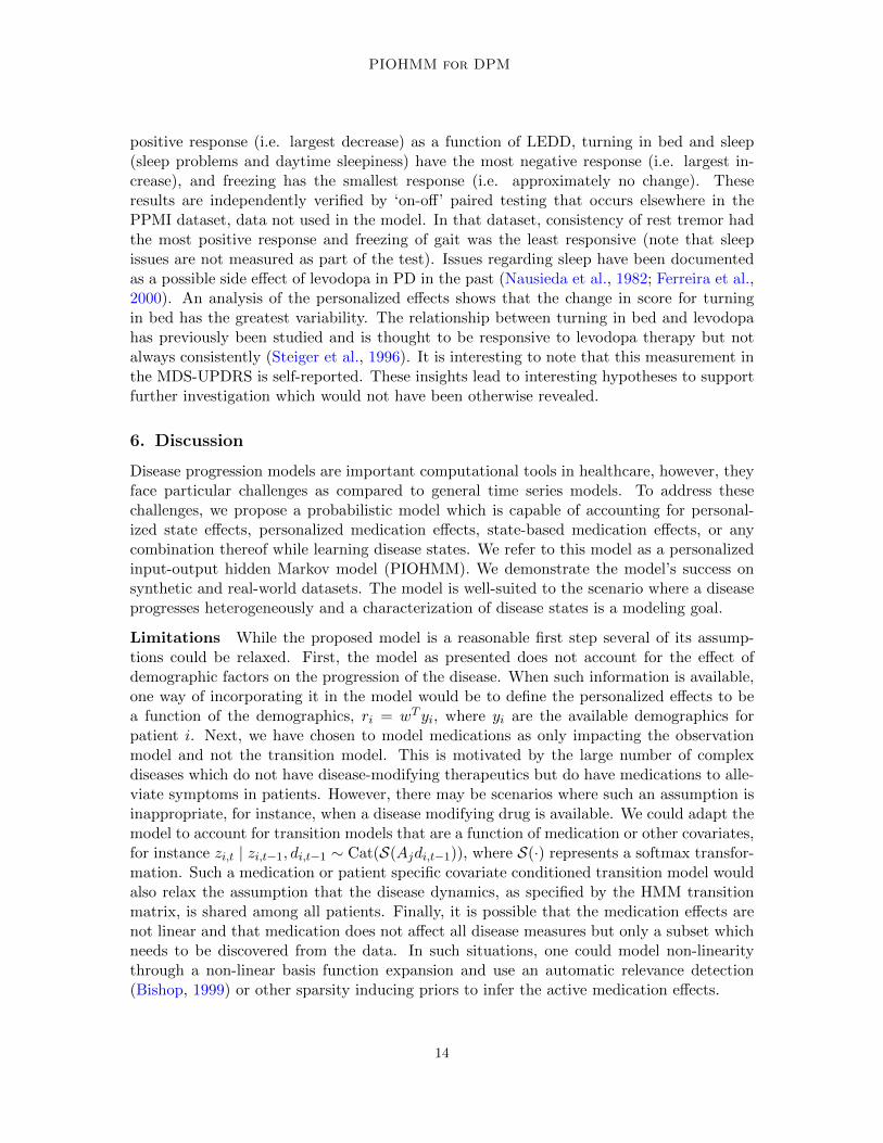
Figure 5: Average of the subitems corresponding to primary PD symptoms from the statemeans, µk. The subscores are calculated using the MDS-UPDRS as follows:tremor, 2.10, 3.15-3.18, postural instability gait, 2.12-2.13, 3.10-3.12, bradykine-sia, 3.4-3.8, 3.14, and rigidity, 3.3. The colors correspond to the range of severitywithin each category (blue for the least severe and red for the most severe) andare redundant with the value in the heatmap.

and postural instability/gait (PI/G). See Figure 5 for a summary. Note that the states areordered in terms of progression, e.g. state 1 cannot transition to state 0, state 2 cannottransition to states 0 or 1, etc. State 1 is the most frequent state at enrollment and has thelowest total MDS-UPDRS score. State 0 has no patients on medication. States 2 and 4 bothhave moderate tremor and are primarily differentiated by which side of the body the diseaseaffects. State 6 has high tremor. States 3, 5, and 7 have increasingly severe gait issues.Per the subtype methodology of Stebbins et al. (2013), which uses MDS-UPDRS subitemsto assign patients who are not on medication to tremor or PI/G subtypes, state 5 is PI/Gdominant, states 0-4 and 6 are tremor dominant, and state 7 is indeterminate. Unlike thesedefinitions, the learned disease states have more granularity and capture severity.

In addition to this static view of the learned states, we are also interested in how thesestates evolve in time. Analysis of the transition probabilities, A, provides insight to expectedtransition patterns. Using the Viterbi algorithm, marginalizing over the personalized effects,we can also estimate the most probable sequence for each patient. As a demonstration ofhow the model could be used, we predict whether a patient in the test dataset will be in atremor dominant or postural instability/gait dominant subtype based on the definitions ofStebbins et al. (2013). To do this, we use the state assignment probabilities at study entryand the transition matrix to calculate state assignment in one year. The probabilities atone year are then used to calculate a weighted average of MDS-UPDRS subitems. Unlikethe states from our model, these literature subtypes are only defined for patients not onmedications, therefore only 24 of the 83 patients in the test set have the required information.Using the model, 17 patients are correctly predicted. If instead we assume that patientsdo not change subtypes from study entry, only 14 patients are correctly predicted. Thisheterogeneity is supported by independent analysis of the PPMI data (Simuni et al., 2016).

We can also analyze the parameters that interact with medication to gain new insights.Overall, facial expression, consistency of rest tremor, and body bradykinesia have the most

13

PIOHMM for DPM

positive response (i.e. largest decrease) as a function of LEDD, turning in bed and sleep(sleep problems and daytime sleepiness) have the most negative response (i.e. largest in-crease), and freezing has the smallest response (i.e. approximately no change). Theseresults are independently verified by ‘on-off’ paired testing that occurs elsewhere in thePPMI dataset, data not used in the model. In that dataset, consistency of rest tremor hadthe most positive response and freezing of gait was the least responsive (note that sleepissues are not measured as part of the test). Issues regarding sleep have been documentedas a possible side effect of levodopa in PD in the past (Nausieda et al., 1982; Ferreira et al.,2000). An analysis of the personalized effects shows that the change in score for turningin bed has the greatest variability. The relationship between turning in bed and levodopahas previously been studied and is thought to be responsive to levodopa therapy but notalways consistently (Steiger et al., 1996). It is interesting to note that this measurement inthe MDS-UPDRS is self-reported. These insights lead to interesting hypotheses to supportfurther investigation which would not have been otherwise revealed.

6. Discussion

Disease progression models are important computational tools in healthcare, however, theyface particular challenges as compared to general time series models. To address thesechallenges, we propose a probabilistic model which is capable of accounting for personal-ized state effects, personalized medication effects, state-based medication effects, or anycombination thereof while learning disease states. We refer to this model as a personalizedinput-output hidden Markov model (PIOHMM). We demonstrate the model’s success onsynthetic and real-world datasets. The model is well-suited to the scenario where a diseaseprogresses heterogeneously and a characterization of disease states is a modeling goal.

Limitations While the proposed model is a reasonable first step several of its assump-tions could be relaxed. First, the model as presented does not account for the effect ofdemographic factors on the progression of the disease. When such information is available,one way of incorporating it in the model would be to define the personalized effects to bea function of the demographics, ri = wT yi, where yi are the available demographics forpatient i. Next, we have chosen to model medications as only impacting the observationmodel and not the transition model. This is motivated by the large number of complexdiseases which do not have disease-modifying therapeutics but do have medications to alle-viate symptoms in patients. However, there may be scenarios where such an assumption isinappropriate, for instance, when a disease modifying drug is available. We could adapt themodel to account for transition models that are a function of medication or other covariates,for instance zi,t | zi,t−1, di,t−1 ∼ Cat(S(Ajdi,t−1)), where S(·) represents a softmax transfor-mation. Such a medication or patient specific covariate conditioned transition model wouldalso relax the assumption that the disease dynamics, as specified by the HMM transitionmatrix, is shared among all patients. Finally, it is possible that the medication effects arenot linear and that medication does not affect all disease measures but only a subset whichneeds to be discovered from the data. In such situations, one could model non-linearitythrough a non-linear basis function expansion and use an automatic relevance detection(Bishop, 1999) or other sparsity inducing priors to infer the active medication effects.

14

PIOHMM for DPM

7. Acknowledgments

The authors would like to thank Mark Frasier for helpful comments and discussion. Dataused in the preparation of this article were obtained from the Parkinson’s Progression Mark-ers Initiative (PPMI) database (www.ppmi-info.org/data). For up-to-date information onthe study, visit www.ppmi-info.org. PPMI – a public-private partnership – is funded by theMichael J. Fox Foundation for Parkinson’s Research and funding partners, including abbvie,Allergan, amathus therapeutics, Avid radiopharmaceuticals, Biogen, BioLegend, Bristol-Myers Squibb, Celgene, Denali, GE Healthcare, Genentech, GlaxoSmithKline, Golub Cap-ital, Handl Therapeutics, insitro, Janssen, Lilly, Lundbeck, Merck, Meso Scale Discovery,Pfizer, Primal, Prevail Therapeutics, Roche, Sanofi Genzyme, Servier, Takeda, Teva, UCB,Verily and Voyager Therapeutics.

References

A.M. Alaa and M. van der Schaar. Attentive state-space modeling of disease progression.In NeurIPS, 2019.

R.M. Altman. Mixed hidden markov models: An extension of the hidden markov modelto the longitudinal data setting. Journal of the American Statistical Association, 102:201–210, 2007.

M. Bachlin, M. Plotnik, D. Roggen, I. Maidan, J. M. Hausdorff, N. Giladi, and G. Troster.Wearbale assistant for Parkinson’s disease patients with freezing of gait symptoms. IEEETransactions on Information Technology in Biomedicine, 14:436–446, 2010.

L. E. Baum. An inequality and associated maximization technique in statistical estimationof probabilistic functions of Markov processes. Inequalities, 3:1–8, 1972.

Y. Bengio and P. Frasconi. An input output HMM architecture. In NIPS, 1995.

C. M. Bishop. Variational principal components. In ICANN, 1999.

Z. Che, S. Purushotham, G. Li, B. Jiang, and Y. Liu. Hierarchical deep generative modelsfor multi-rate multivariate time series. In ICML, 2018.

P. Eulenberg, N. Kohler, T. Blasi, A. Filby, A.E. Carpenter, P. Rees, F.J. Theis, and F. A.Wolf. Reconstructing cell cycle and disease progression using deep learning. NatureCommunications, 8:1–6, 2017.

J. J. Ferreira, M. Galitzky, J. L. Montastruc, and O. Rascol. Sleep attacks and Parkinson’sdisease treatment. The Lancet, 355:1333–1334, 2000.

J. Futoma, M. Sendak, C. B. Cameron, and K. Heller. Predicting disease progression witha model for multivariate longitudinal clinical data. In Machine Learning for Healthcare,2016.

C. G. Goetz, B. C. Tilley, S. R. Shaftman, and et al. Movement Disorder Society-sponsoredrevision of the Unified Parkinson’s Disease Rating Scale (MDS-UPDRS): Scale presenta-tion and clinimetric testing results. Movement Disorders, 23:2129–2170, 2008.

15

PIOHMM for DPM

C. Guihenneuc-Jouyaux, S. Richardson, and I. M. Longini Jr. Modeling markers of diseaseprogression by a hidden Markov process: Application to characterizing cd4 cell decline.Biometrics, 56:733–741, 2000.

C. H. Jackson, L. D. Sharples, S. G. Thompson, S. W. Duffy, and E. Couto. MultistateMarkov models for disease progression with classification error. Journal of the RoyalStatistical Society: Series D, 52:193–209, 2003.

J. Jankovic. Parkinson’s disease: Clinical features and diagnosis. Journal of Neurology,Neurosurgery & Psychiatry, 79:368–376, 2008.

A. A. Kehagia, R. A. Barker, and T. W. Robbins. Neuropsychological and clinical hetero-geneity of cognitive impairment and dementia in patients with Parkinson’s disease. TheLancet Neurology, 9:1200–1213, 2010.

D.P. Kingma and J.L. Ba. ADAM: A method for stochastic optimization. In ICLR, 2015.

M. Lorenzi, M. Filipponse, G. B. Frisoni, D. C. Alexander, and S. Ourselin. Probabilis-tic disease progression modeling to characterize diagnostic uncertainty: Application tostaging and prediction in Alzheimer’s disease. NeuroImage, 190:56–68, 2019.

K. Marek, D. Jennings, S. Lasch, and et al. The Parkinson’s Progression Marker Initiative(PPMI). Progress in Neurobiology, 95:629–635, 2011.

D. R. Mould. Models for disease progression: New approaches and uses. Clinical Pharma-cology & Therapeutics, 92:125–131, 2012.

P. A. Nausieda, W. J. Weiner, L. R. Kaplan, S. Weber, and H. L. Klawans. Sleep disruptionin the course of chronic levodopa therapy: An early feature of the levodopa psychosis.Clinical Neruopharmacology, 5:183–194, 1982.

T. Pham, T. Tran, D. Phung, and S. Venkatesh. Predicting healthcare trajectories frommedical records: A deep learning approach. Journal of Biomedical Informatics, 69:218–229, 2017.

R. B. Postuma, D. Berg, M. Stern, and et al. MDS clinical diagnostic criteria for Parkinson’sdisease. Movement Disorders, 30:1591–1601, 2015.

L. R. Rabiner. A tutorial on hidden Markov models and selected applications in speechrecognition. In IEEE, 1989.

P. Schulam and S. Saria. A framework for individualizing predictions of disease trajectoriesby exploiting multi-resolution structure. In NIPS, 2015.

T. Simuni, C. Caspell-Garcia, C. Coffey, S. Lasch, C. Tanner, K Marek, and PPMI. Howstable are parkinson’s disease subtypes in de novo patients: Analysis of the ppmi cohort?Parkinsonism and Related Disorders, 28:62–67, 2016.

16

PIOHMM for DPM

G. T. Stebbins, C. G. Goetz, D. J. Burn, J. Jankovic, T. K. Khoo, and B. C. Tilley.How to identify tremor dominant and postural instability/gait difficulty groups with themovement disorder society unified Parkinson’s disease rating scale: Comparison with theunified Parkinson’s disease rating scale. Movement Disorders, 28:668–670, 2013.

M. J. Steiger, P. D. Thompson, and C. D. Marsden. Disordered axial movement in Parkin-son’s disease. Journal of Neurology, 61:645–648, 1996.

R. Sukkar, E. Katz, Y. Zhang, D. Raunig, and B. T. Wyman. Disease progression mod-eling using hidden Markov models. In Annual International Conference of the IEEEEngineering in Medicine and Biology Society, 2012.

Z. Sun, S. Ghosh, Y. Li, Y. Cheng, A. Mohan, C. Sampaio, and J. Hu. A probabilistic dis-ease progression modeing approach and its application to integrated Huntington’s diseaseobservational data. JAMIA Open, 2:123–130, 2019.

N. Tangri, L. A. Stevens, J. Griffith, H. Tighiouart, O. Djurdjev, D. Naimark, A. Levin,and A. S. Levey. A predictive model for progression of chronic kideny disease to kidneyfailure. JAMA, 305:1553–1559, 2011.

C. L. Tomlinson, R. Stowe, S. Patel, C. Rick, R. Gray, and C. E. Clarke. Systematic reviewof levodopa dose equivalency reporting in Parkinson’s disease. Movement Disorders, 25:2649–2685, 2010.

C. V. M. Verschuur, S. R. Suwijn, J. A. Boel, and et al. Randomized delayed-start trial oflevodopa in Parkinson’s disease. New England Journal of Medicine, 380:315–324, 2019.

X. Wang, D. Sontag, and F. Wang. Unsupervised learning of disease progression models.In KDD, 2014.

W. J. Zetusky, J. Jankovic, and F. J. Pirozzolo. The heterogeneity of Parkinson’s disease.Neurology, 35:522, 1985.

Appendix A. Forward-backward algorithm details

The application of the forward-backward algorithm follows the steps of the forward-backwardalgorithm as applied to an HMM. We define

γ(zi,t) = p(zi,t | xi,mi, ri) =p(xi,1, . . . , xi,t, zi,t | mi, ri)p(xi,t+1, . . . , xi,T | zi,t,mi, ri)

p(xi | mi, ri)(15)

Further, we defineα(zi,t) = p(xi,1 . . . , xi,t, zi,t | mi, ri)

β(zi,t) = p(xi,t+1, . . . , xi,T | zi,t,mi, ri)(16)

17

PIOHMM for DPM

α(zi,t) = p(xi,1 . . . , xi,t, zi,t | mi, ri) (17)

= p(xi,1 . . . , xi,t | zi,t,Mi)p(zi,t | mi, ri) (18)

= p(xi,t | zi,t,mi, ri)p(xi,1 . . . , xi,t−1 | zi,t,mi, ri)p(zi,t | mi, ri) (19)

= p(xi,t | zi,t,mi, ri)p(xi,1 . . . , xi,t−1, zi,t | mi, ri) (20)

= p(xi,t | zi,t,mi, ri)∑zi,t−1

p(xi,1 . . . , xi,t−1, zi,t−1, zi,t | mi, ri) (21)

= p(xi,t | zi,t,mi, ri)∑zi,t−1

p(xi,1 . . . , xi,t−1, zi,t | zi,t−1,mi, ri)p(zi,t−1 | mi, ri) (22)

= p(xi,t | zi,t,mi, ri)∑zi,t−1

p(xi,1 . . . , xi,t−1 | zi,t−1,mi, ri)p(zi,t | zi,t−1,mi, ri)p(zi,t−1 | mi, ri)

(23)

= p(xi,t | zi,t,mi, ri)∑zi,t−1

p(xi,1 . . . , xi,t−1, zi,t−1 | mi, ri)p(zi,t | zi,t−1,mi, ri) (24)

= p(xi,t | zi,t,mi, ri)∑zi,t−1

α(zi,t−1)p(zi,t | zi,t−1) (25)

Similarly,

β(zi,t) = p(xi,t+1, . . . , xi,T | zi,t,mi, ri) (26)

=∑zi,t+1

p(xi,t+1, . . . , xi,T , zi,t+1 | zi,t,mi, ri) (27)

=∑zi,t+1

p(xi,t+1, . . . , xi,T | zi,t, zi,t+1,mi, ri)p(zi,t+1 | zi,t,mi, ri) (28)

=∑zi,t+1

p(xi,t+1, . . . , xi,T | zi,t+1,mi, ri)p(zi,t+1 | zi,t,mi, ri) (29)

=∑zi,t+1

p(xi,t+2, . . . , xi,T | zi,t+1,mi, ri)p(xi,t+1 | zi,t+1,mi, ri)p(zi,t+1 | zi,t,mi, ri)

(30)

=∑zi,t+1

β(zi,t+1)p(xi,t+1 | zi,t+1,mi, ri)p(zi,t+1 | zi,t) (31)

The recursion is started using

α(zi,1) = p(zi,1)p(xi,1, | zi,1, di,1,mi, ri) =k∏k=1

{πkp(xi,1 | di,1, φk,mi, ri)]}zi,1=k (32)

andβ(zi,T ) = 1 (33)

18

PIOHMM for DPM

The objective function can be expanded and written

L =

N∑i=1

K∑k=1

ln p(zi,1 = k | πk)q(zi,1 = k | xi,mi, ri)+

K∑k=1

K∑j=1

T∑t=2

N∑i=1

ln p(zi,t = k | zi,t−1 = j, Ajk)q(zi,t = k, zi,t−1 = j | xi,mi, ri)+

N∑i=1

∫ln p(mi | σ2m)q(mi)dmi +

N∑i=1

∫ln p(ri | σ2r )q(ri)dri+

N∑i=1

K∑k=1

[ ∫ ∫ T∑t=1

ln p(xi,t | zi,t = k, φk, vk, di,t,mi, ri)q(mi)dmiq(ri)dri

]q(zi,t = k | xi,mi, ri)−

N∑i=1

∫q(mi) ln q(mi)dmi −

N∑i=1

∫q(ri) ln q(ri)dri−

N∑i=1

K∑k=1

∫ ∫q(mi)q(ri)q(zi,1 | xi,mi, ri) ln q(zi,1 | xi,mi, ri)dmidri−

N∑i=1

T∑t=2

K∑k=1

K∑j=1

∫ ∫q(mi)q(ri)q(zi,t, zi,t−1 | xi,mi, ri) ln q(zi,t | zi,t−1,mi, ri)dmidri

(34)

Appendix B. Fixed point updates

The equations for the parameter updates under the observation model

xi,t | zi,t = k, di,t ∼ N (µk + ri + (vk +mi)di,t,Σk) (35)

19

PIOHMM for DPM

Figure 6: Distributions of the index of the last observed visit and the number of observationsper patient. Not all visits for a trajectory may be observed. The left histogramrepresents the time point of the final observation for each patient in the trainingset and the right histogram represents the number of observed visits. This is aresult of the observation protocol. The testing data is distributed similarly.

are shown below.

π =

∑Ni=1 γ(zi,1 = k)∑N

i=1

∑Kk=1 γ(zi,1 = k)

Ajk =

∑Ni=1

∑Tt=2 ξ(zi,t−1 = j, zi,t = k)∑N

i=1

∑Tt=2

∑Kk=1 ξ(zi,t−1 = j, zi,t = k)

µk =

∑Ni=1

∑Tt=1 γ(zi,t = k)(xi,t − rsi − (vk +ms

i )di,t)∑Ni=1

∑Tt=1 γ(zi,t = k)

Σk =

∑Ni=1

∑Tt=1 γ(zi,t = k)skits

Tkit∑N

i=1

∑Tt=1 γ(zi,t = k)

skit = xi,t − µk − rsi − (vk +msi )di,t

vk =

[( N∑i=1

T∑t=1

d2i,tγ(zi,t = k))ID +

1

σ2vΣk

]−1[ N∑i=1

T∑t=1

γ(zi,t = k)(xi,t − µk − rsi −msidi,t)di,t

]

σ2m =1

ND

N∑i=1

(msi )

Tmsi

σ2r =1

ND

N∑i=1

(rsi )Trsi

Appendix C. Parkinson’s disease patient cohort

C.1. Data availability

Figure 6 shows the distribution of the number of visits per patient. On average, data isobserved up to visit 21, although each visit within the trajectory is not necessarily observed.The average number of observations per patient is 12.

20

PIOHMM for DPM

Figure 7: Trends of total number of observations with various patient attributes. Time sinceenrollment is strongly correlated with the total number of observations whereasmeasures of disease state are not.

C.2. Missing data analysis

Although there is no robust test to confirm that data is not missing at random, empiricalevidence suggests this is not the case for the PPMI PD dataset. We show the trends innumber of total observations as a function of time since study enrollment as well as MDS-UPDRS total and change in MDS-UPDRS total in Figure 7. If data were not missing atrandom, we might hypothesize that patients who have high MDS-UPDRS total values atlast visit or patients who have large increases in MDS-UPDRS would have a small numberof visits due to study drop-out. For the most part, we do not observe any linear trend(r2 = 0.01 for total and r2 = 0 for change), whereas there is a strong linear trend in therelationship between time since enrollment and number of visits (r2 = 0.83). Althoughinconclusive, we take this to imply that a majority of missingness is due to the studyprotocol and not censoring or drop-out as a function of disease state.

21