Rollout Strategy for Hidden Markov Model (HMM)-based

Dynamic Sensor Scheduling Hyunsung Lee, Satnam Singh, Woosun An, Swapna S. Gokhale, Krishna Pattipati and

David L. Kleinman

Abstract— In this paper, a hidden Markov model (HMM)-based dynamic sensor scheduling problem is formulated, and solved using rollout concepts to overcome the computational intractability of the dynamic programming (DP) recursion. The problem considered here involves dynamically sequencing a set of sensors to minimize the sum of sensor cost and the HMM state estimation error cost. The surveillance task is modeled as a single HMM with multiple emission matrices corresponding to each of the sensors. The rollout information gain (RIG) algorithm proposed herein employs the information gain (IG) heuristic as the base algorithm. The RIG algorithm is illustrated on an intelligence, surveillance, and reconnaissance (ISR) scenario of a village for the presence of weapons and terrorists/refugees. Extension of the RIG strategy to monitor multiple HMMs involves combining the information gain heuristic with the auction algorithm that computes the κ -best assignments at each decision epoch of rollout.

I. INTRODUCTION

A. Motivation The dynamic sensor scheduling problem occurs in a

number of applications, including target tracking, sensor networks, unmanned aerial vehicles for surveillance in remote or hostile environments, robotics, and supply chain management in a warehouse. In a target tracking application, sensors are dynamically activated to trade off tracking performance with the sensor usage cost [1]. For example, consider a target identification scenario where an incoming aircraft needs to be identified as an enemy or as a friendly target using various forms of sensors available at a base station [2]. This scenario requires sensor scheduling because the better sensors (e.g., radar) tend to reveal or to provide clues about the location of the aircraft relative to the base station, whereas the more stealthy sensors tend to be inaccurate [2].

In this paper, we motivate the sensor scheduling problem to support an intelligence, surveillance, and reconnaissance

(ISR) officer in an expeditionary strike group (ESG) mission in coordinating the use of surveillance assets (sensors) to improve situational awareness [3]. An ESG provides a flexible force package, capable of tailoring itself to a wide variety of mission sets [3]. An important ESG mission involves dealing with asymmetric threats, such as terrorist groups who carry out attacks while trying to avoid direct confrontation. Terrorist groups are elusive, secretive, amorphously structured and decentralized entities that often appear unconnected. This stealthy behavior makes it very difficult to predict when and where they will strike. Moreover, the increased geographical range and unpredictable nature of this behavior require effective allocation and appropriate scheduling of sensors to achieve mission objectives. Effectively performing the ISR activities is a key step to gain situational awareness, which, in turn, enables the allocation of resources for the interdiction of terrorist activities.

Manuscript received March 29, 2007. The study reported in this paper was

supported, in part, by the Office of Naval Research under contract no. 00014-00-1-0101. Any opinions expressed in this paper are solely those of the authors and do not represent those of the sponsor.

Hyunsung Lee, Satnam Singh, Woosun An, and Krishna Pattipati are with the Electrical and Computer Engineering Department, University of Connecticut, CT , USA (e-mail:krishna@engr.uconn.edu).

Swapna S. Gokhale is with the Computer Science and Engineering Department, University of Connecticut, CT , USA.

David L. Kleinman is with the Naval Postgraduate School, Monterey, CA, USA.

We model the asymmetric threats using hidden Markov models, because these activities are concealed and their true state can be only inferred through the observations obtained using various ISR sensors. A pattern of these observations and its dynamic evolution over time is a potential realization of an asymmetric threat [4]. Performing the ISR activities requires multiple sensors to provide observations needed for accurately estimating the status of suspicious activities. The available sensors are limited in number, and possess different attributes (e.g. cost, deployment requirements, accuracy, capabilities, etc.) requiring judicious sensor allocation over time. For example, unmanned aerial vehicles (UAVs) are preferred assets for monitoring nearly all the ISR activities; however, they cannot be deployed in large numbers due to their limited availability. Therefore, an effective scheduling of ISR sensors over time is essential for accurate situation assessment and to the success of the overall mission.

B. Previous Work Sensor scheduling problem has been widely studied in the

area of target tracking (e.g. [1], [2]). In [5], Singh et al. provided a summary of previous research on sensor scheduling for targets, whose dynamics are modeled by linear Gauss-Markov processes. They formulated the sensor scheduling problem as one of minimizing the variance of the estimation error of the hidden states of a controlled HMM with respect to a given action sequence [5]. The authors proposed a stochastic gradient algorithm to determine the optimal schedule for a HMM where the state, observation and action spaces are continuous. Another effort, related to our

work, using the discrete HMM framework was presented by Krishnamurthy in [2]. In this case, the author proposed a stochastic dynamic programming (DP) framework to solve the sensor scheduling problem. Logethitis et al. [6] formulated the sensor scheduling problem as computing a sequence of active sensors to maximize the information on the state of the system.

Rollout algorithms were first proposed for the approximate solution of dynamic programming recursions by Bertsekas et al. in [7], [8]. They are a class of suboptimal solution methods inspired by the policy iteration of dynamic programming and the approximate policy iteration of neuro-dynamic programming. The rollout algorithm combined with the information gain heuristic (RIG) was first proposed in our previous research on sequential fault diagnosis [9]. In [9], we showed that rollout strategy, which can be combined with the one-step or multi-step lookahead heuristic algorithms as base algorithms, can solve test sequencing problems in real-world systems with a higher computational efficiency than the optimal strategies, while being superior to those using the base algorithms only. In this paper, we apply the RIG algorithm to solve the dynamic sensor scheduling problem.

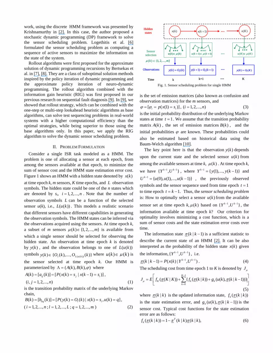
II. PROBLEM FORMULATION Consider a single ISR task modeled as a HMM. The

problem is one of allocating a sensor at each epoch, from among the sensors available at that epoch, to minimize the sum of sensor cost and the HMM state estimation error cost. Figure 1 shows an HMM with a hidden state denoted by ( )x k at time epoch k, m sensors, K time epochs, and observation symbols. The hidden state could be one of the n states which are denoted by s

L

i, .1, 2,...,i = n

m

Note that the number of observation symbols L can be a function of the selected sensor u(k), i.e., . This models a realistic scenario that different sensors have different capabilities in generating the observation symbols. The HMM states can be inferred via the observations acquired using the sensors. At time epoch k, a subset of m sensors

( ( ))L u k

( ) {1, 2,..., }kµ ∈ is available from which a single sensor should be selected for observing the hidden state. An observation at time epoch k is denoted by , and the observation belongs to one of symbols where

( )y k ( ( ))L u k)}(),....,({)( ))((1 kOkOky kuL∈ )()( kku µ∈ is

the sensor selected at time epoch k. Our HMM is parameterized by ( ( ), ( ), )A k B k ϕΛ = where

( ) [ ( )] [ ( ( ) | ( 1) )]ij j iA k a k P x k s x k s= = = − = ,

( , 1, 2,..., )i j n= (1)

is the transition probability matrix of the underlying Markov chain,

( ) [ ( )] [ ( ( ) ( ) | ( ) , ( ) ]liq l iB k b k P y k O k x k s u k q= = = = = , ( ; ; ) (2) 1,2,...,i n= 1, 2,...,l L= 1, 2,...,q = m

( ) ( )ly k O k= ( ) ( )ly K O K=Observations

Hiddenstates

Sensorselection

( )x k ( 1)x k + ( )x K

( ) ( )u k kµ∈ ( 1) ( 1)u k kµ+ ∈ + ( ) ( )u K Kµ∈

Time k k+1 K

( 1) ( 1)ly k O k+ = +

( ) {1, 2, ..., }k mµ ⊂

( ) ( )ly k O k= ( ) ( )ly K O K=Observations

Sensorselection

( )x k ( 1)x k + ( )x KHiddenstates

( ) ( )u k kµ∈( ) ( )u k kµ∈ ( 1) ( 1)u k kµ+ ∈ + ( ) ( )u K Kµ∈

Time k k+1 K

( 1) ( 1)ly k O k+ = +

( ) {1, 2, ..., }k mµ ⊂

Fig. 1. Sensor scheduling problem for single HMM

is the set of emission matrices (also known as confusion and observation matrices) for the m sensors, and

[ ( (1) )]i ip x sϕ ϕ= = = ( 1,2,..., )i n, = (3) is the initial probability distribution of the underlying Markov states at time 1t = . We assume that the transition probability matrix ( )A k , the set of emission matrices , and the initial probabilities

( )B kϕ are known. These probabilities could

also be estimated based on historical data using the Baum-Welch algorithm [10].

The key point here is that the observation depends upon the current state and the selected sensor from among the available sensors at time k,

( )y k( )u k

( )kµ . At time epoch k,

we have , where Y y and

, the previously observed symbols and the sensor sequence used from time epoch

1 1{ ,k kY U− − } y k− = −kU u u u k− = −

1 { (1),..., ( 1)}k

1 { (0), (1),..., ( 1)}1t =

to time epoch t k 1.= − Thus, the sensor scheduling problem is: How to optimally select a sensor u k from the available

sensor set at time epoch k,

( )

( )kµ based on { , , the information available at time epoch k? Our criterion for optimality involves minimizing a cost function, which is a sum of sensor costs and the state estimation error costs over time.

1 1}k kY U− −

The information state ( | 1)k kπ − is a sufficient statistic to describe the current state of an HMM [2]. It can be also interpreted as the probability of the hidden state ( )x k

}k kY U− −

given

the information,{ , , i.e. 1 1

1 1( | 1) ( ( ) | , )k kk k P x k Y Uπ − −− = . (4) The scheduling cost from time epoch 1 to K is denoted by Jµ

1

0

( ( | )) { ( ( | )) ( ( ), ( | 1))}K

K k kk

J E f K K f k k g u k k kµ π π π−

=

⎡ ⎤= + + −⎢ ⎥⎣ ⎦

∑ (5) where ( | )k kπ is the updated information state, ( ( | ))kf k kπ is the state estimation error, and ( ( ), ( | 1))kg u k k kπ − is the sensor cost. Typical cost functions for the state estimation error are as follows:

( ( | )) 1 ( | ) ( | ),Tkf k k k k k kπ π π= − (6)

( ( | )) 1 max ( | ),k iif k k k kπ π= − (7)

Step 1: Predict the information state using (15) as described in Section IV. Step 2: Compute the information gain per unit cost of a sensor given in (13) for all m sensors at time k. Step 3: Select top κ sensors which maximize the information gain per unit cost given in (13). Usually, κ is in the range [2,5] to avoid excessive rollouts. Step 4: Compute the total scheduling cost as defined in (5) for the top κ sensors. Select the sensor which minimizes the cost as given by (12). Step 5: Update time epoch and go back to Step 1 until k K

1k k← += .

1 1( ( | )) min ( | ) .

n

k ji n jf k k k k ijπ π

≤ ≤=

= ∑ λ (8)

The first criterion can interpreted as an L2 norm of the state estimation error, the second as the error probability of a maximum a posteriori probability-based decision rule, and the third as the expected cost of errors in estimating the information state, respectively. In (8), ijλ represents the cost of erroneously estimating the hidden state as sj when the true state is si. The sensor cost is sum of sensor usage cost and sensor moving cost i.e.

( ( ), ( | 1)) ( ( ), ( | 1)) ( ( ))k k mg u k k k h u k k k c u kπ π− = − + (9) where the sensor usage cost is,

1

( ( ), ( | 1)) ( , ( )) ( | 1)n

k k ii

h u k k k c s u k k kπ π=

− = −∑ i

( ( )) ( | 1)Tkc u k k kπ= − (10)

and ( )1 2( ( )) ( , ( )), ( , ( )),..., ( , ( ))Tk nc u k c s u k c s u k c s u k= is the

usage cost of sensor associated with each HMM state( )u k is . We also considered the cost of moving a sensor c u , which is computed for sensor as:

( ( ))m k( )u k

2( ) ( )||( , ) ( , ) ||( ( )) ( ( ))

v(u(k))o o u k u k L

m

a b a bc u k w u k

−= (11)

where and denotes the cartesian coordinates of the sensor monitoring place and the selected sensor respectively. Here, w u indicates the priority and

denotes the velocity of the sensor.

0 0( , )a b ( ) ( )( ,u k u ka b )

k( ( ))v( ( ))u k

The optimum solution to the sensor scheduling problem is the sensor sequence * *K Kq U= which minimizes the sensor scheduling cost as defined in (5). Formally,

0

* *

{ ( ) ( )}min

Kk

K K

u k kq U Jµ

µ =∈= = (12)

The optimal solution of (5) can be obtained using the dynamic programming (DP) technique; however, the computational complexity is , which is exponential in D, the number of quantization levels used to discretize the continuous-valued information state. Here, n is the number of states in a HMM, m is the number of sensors, L is the maximum number of observation symbols, and K is the number of time epochs. Hence, the DP technique is impractical for an HMM containing more than around 15 states [2]. This motivates us to investigate suboptimal algorithms designed to solve the sensor scheduling problem containing hundreds of HMM states. We propose the rollout information gain (RIG) algorithm with computational complexity of O per rollout, which is significantly lower than the DP technique.

1( nO D mnLK− )

)mnLK(

Sensors/assets

23

1

m

Process k = 2 to K

Process k = 1 to K

Select top 2 sensors according to information gain heuristic

Process k = 3 to K

Top 2 sensors

1k =

4

2k = 3k = k K=Time

m-1

Sensors/assets

23

1

m

Process k = 2 to K

Process k = 1 to K

Select top 2 sensors according to information gain heuristic

Process k = 3 to K

Top 2 sensors

1k =

4

2k = 3k = k K=Time

m-1

k=

Fig. 2. Rollout information gain (RIG) algorithm

Fig. 3. Pseudo code for the rollout information gain (RIG) algorithm

III. ROLLOUT ALGORITHM Rollout algorithms are a class of suboptimal methods

which are capable of improving the effectiveness of any given heuristic through sequential application. This is due to the policy improvement mechanism of the underlying policy iteration process [9]. They can be viewed as a single step of the classical policy iteration method, wherein we start from a given easily implementable and computationally tractable policy, and then try to improve on that policy using online learning and simulation. The attractive aspects of rollout algorithms are simplicity, broad applicability, and suitability for online implementation. The details of the rollout algorithms are provided in [7]-[9].

To solve the sensor scheduling problem, we combine the rollout method with the information gain heuristic. Figure 2 graphically illustrates the RIG algorithm with two rollouts at each time epoch. Figure 3 shows the pseudo code of the rollout information gain (RIG) algorithm.

IV. COMBINING ROLLOUT ALGORITHM WITH INFORMATION GAIN HEURISTIC

The information heuristic selects a sensor q u in the predicted information state

* * ( )( | 1)i k kπ − that maximizes

*( 1)u k −

( 1)x k − ( )x k ( 1)x k +Hiddenstates

Selectwith max (I)

Observe ( 1)y k −with

Estimate( 1 | 1)k kπ − −

Observe ( )y kwith

Estimate( | )k kπ

Selectwith max (I)

Observe ( 1)y k +with

Estimate( 1 | 1)k kπ + +

Selectwith max (I)

( 1)u k − ( )u k ( 1)u k +Predict

( | 1)k kπ −

Predict

( 1| )k kπ +

SensorSelection

Measurement

Measurementupdate

Step 1 Step 2

Step 3

Step 4

*( )u k *( 1)u k +*( 1)u k −

( 1)x k − ( )x k ( 1)x k +Hiddenstates

Selectwith max (I)

Observe ( 1)y k −with

Estimate( 1 | 1)k kπ − −

Observe ( )y kwith

Estimate( | )k kπ

Selectwith max (I)

Observe ( 1)y k +with

Estimate( 1 | 1)k kπ + +

Selectwith max (I)

( 1)u k − ( )u k ( 1)u k +Predict

( | 1)k kπ −

Predict

( 1| )k kπ +

SensorSelection

Measurement

Measurementupdate

Step 1 Step 2

Step 3

Step 4

*( )u k *( 1)u k +

Fig. 4. Information gain (IG) heuristic steps for sensor scheduling

State 1:Normal

State 2: Terrorists disguised

as refugees

State 3: Weapons

State4:Pacified village

0.9

0.1

0.7

0.3

0.6

0.4

0.80.2

Assets SH-60 E2-C UAV P3 AV-8B MEU

State 1:Normal

State 2: Terrorists disguised

as refugees

State 3: Weapons

State4:Pacified village

0.9

0.1

0.7

0.3

0.6

0.4

0.80.2

Assets SH-60 E2-C UAV P3 AV-8B MEU

Fig. 5. A fishing village scenario for sensor scheduling problem

the information gain (IG) per unit cost of a sensor:

* *

( )

( ( | -1), ( ) )( ) arg max ( ( ), ( | 1))q k k

I k k u k qq u kg u k k kµ

ππ∈

== =

− (13)

where ( ( ), ( | 1))kg u k k kπ − is the sensor cost as defined in (9) and ( ( | -1), ( ) )I k k u k qπ = is the information gain given by:

21 1

( ( | -1), ( ) ) = ( | 1) ( ) log ( ) -n L

i liq liqi l

I k k u k q k k b k b kπ π= =

= −∑ ∑

21 1 1

( ( ) ( | 1)) log ( ( ) ( | 1))L n n

liq i liq il i i

b k k k b k k kπ π= = =

− −∑ ∑ ∑ . (14)

The derivation of information gain is provided in the Appendix. The information heuristic algorithm is a terminating and sequentially improving one step lookahead procedure [9]. In the context of sensor scheduling problem, the information gain (IG) heuristic algorithm consists of the following four steps (Figure 4):

Step 1 (State Prediction): In this step, we predict the information state vector ( | 1)k kπ − for the next sampling epoch k using the current information state update

( 1 | 1)k kπ − − and the transition matrix ( )A k as follows:

( | 1) ( ) ( 1| 1)Tk k A k k kπ π− = − − . (15) Here, the current information update ( 1 | 1)k kπ − − uses the

information available up to time k-1, i.e., where

and are the observation sequence and the sensor sequence upto and including time k-1, respectively.

1 1{ ,k kY U− − }

−1 { (1),..., ( 1)}kY y y k− = − 1 { (0), (1),..., ( 1)}kU u u u k− =

Step 2 (Sensor Selection): We compute the information gain ( ( | -1), ( ) )I k k u k qπ = for all the m sensors using (14).

Select a sensor that maximizes the information

gain per unit cost as given in (13).

* * ( )q u k=

Step 3 (Observation): The new observation ( ) ( )ly k O k=

is obtained using the sensor according to the emission probability matrix given in (2).

* ( )u k

Step 4 (Observation Update): The updated state at the next time ( | -1)i k kπ is obtained using the forward algorithm [12] as follows:

*

*

1

( ) ( | 1)( | )

( ) ( | 1)

iliqi n

jljqj

b k k kk k

b k k k

ππ

π=

−=

−∑. (16)

V. SIMULATIONS AND RESULTS We consider a scenario where an ISR officer needs to

dynamically allocate sensors to monitor asymmetric threat activities in a notional area that involves primarily the fictitious countries of Asiland and Bartola [3]. The northern shore of Asiland was struck by a tsunami that caused massive losses to her civilian populace. Large numbers of Asiland refugees fled and crossed the strait to fishing villages and refugee camps in Bartola seeking help and assistance. Insurgents and terrorist factions in Asiland began to take advantage of the situation, move their operations into Bartola by intermingling with the refugees and smuggling weapons onboard fishing boats and merchant ships.

The problem of monitoring for the presence of terrorists and weapons in a fishing village of Bartola is modeled using a four state HMM. Activities such as the presence of terrorists and weapons, and to learn the crowd demeanor (normal or protesters or terrorists) are continually monitored using the following six sensors: SH-60, E2-C, UAV, P3, AV-8B and MEU. As shown in Figure 5, state 1 represents the normal state of crowd in the fishing village. In state 2, refugees move into the village. Terrorists disguised as refugees arrive in the village and they also smuggle weapons into the village; this is modeled as state 3. In state 4, the weapons and terrorists are prosecuted/pacified and the village resumes normalcy, which is modeled by a transition to state 1.

In this scenario, there are several sensors capable of performing ISR and they have different speeds and capabilities. The scenario assumes 4 observation symbols for each sensor; the symbols provide information on the state of threat activity in the fishing village. We use nominal values of the transition probabilities for the sake of illustration, which are shown in Figure 5. The emission probabilities were also set to their nominal values and varied as a function of sensor accuracy variable p to analyze the robustness of the algorithm for various sensor accuracies. The cost function in (5) employed the state estimation error criterion in (6). The sensor scheduling cost considered in the fishing village scenario is:

0 0.05 0.1 0.15 0.245

50

55

60

65

70

75

Variable p

Tota

l sch

edul

ing

cost

RIGIGSensor 6Sensor 5

Fig. 6. Variation of the total scheduling cost with variable p

1

0

[ {1 ( | )} ( | )

{1 ( | )} ( | )

T

KT

k

J E K K K

k k k k

µ β π π

β π π−

=

= −

+ −∑

K

1

0

{ ( ( )) ( ( )} ( | 1)]K

T Tk m

k

c u k c u k k kπ−

=

+ +∑ − (17)

where ( ( ))Tkc u k and ( ( ))T

mc u k are the costs associated with sensor usage cost and moving the sensor as given in (10) and (11), respectively. For simulations, we set the weighted priority vector ( ( )) [1,2,3,4,1,1]Tw u k = , 10β = , and the total number of time epochs . The velocities of the six sensors are set as

5K =T v (u(k)) [200,450,300,100,500,80]= . The

sensor usage costs are selected as ( ( )) [4,11,8,5,6.5,2]Tkc u k = .

Figure 6 shows the total scheduling cost averaged over 1000 Monte Carlo runs. To check the robustness of the algorithm, the cost was obtained by varying the observation probability using the variable p. Here, Sensor 5 or Sensor 6 curves indicate the static scheduling i.e. the cost was obtained by using sensor 5 or sensor 6 for all time epochs. Sensor scheduling via the rollout information gain algorithm (RIG) has approximately 9~10% lower cost as compared to one using only the information gain heuristic (IG) and ≈ 42% lower cost as compared to static scheduling (sensor 6). The dual advantage of using rollout information gain (RIG) algorithm is that it significantly reduces the complexity of dynamic programming, while improving the accuracy over the base heuristic, information gain.

VI. SENSOR SCHEDULING FOR MULTIPLE HMMS In this section, we will briefly explain how the single

HMM sensor scheduling problem can be extended to multiple HMMs. A simple example of sensor scheduling with multiple HMMs involves a scenario where we need to simultaneously

HMM (2)

HMM (1)

HMM (N)

Time k k+1 K

Observations

1 ( 1)x k +1 ( )x k 1 ( )x K

2 ( )x K2 ( 1)x k +2 ( )x k

( )Nx k ( 1)Nx k + ( )Nx K

( 1)y k + ( )y K( )y k

Sensorselection

( ) {1, 2, ..., }k mµ ⊂

( ) ( )u k kµ∈ ( 1) ( 1)u k kµ+ ∈ + ( ) ( )u K Kµ∈

HMM (2)

HMM (1)

HMM (N)

Time k k+1 K

Observations

1 ( 1)x k +1 ( )x k 1 ( )x K

2 ( )x K2 ( 1)x k +2 ( )x k

( )Nx k ( 1)Nx k + ( )Nx K

( 1)y k + ( )y K( )y k

Sensorselection

( ) {1, 2, ..., }k mµ ⊂

( ) ( )u k kµ∈( ) ( )u k kµ∈ ( 1) ( 1)u k kµ+ ∈ + ( ) ( )u K Kµ∈( ) ( )u K Kµ∈

Fig. 7. Sensor scheduling problem for multiple HMMs

monitor the threat activities that are dispersed geographically in a region. Figure 7 shows the sensor scheduling problem with m sensors and N surveillance tasks modeled using N HMMs. The information gain for each sensor-HMM pair is computed, and the sensors are assigned to HMMs using the κ-best version of the auction algorithm [11], [13]. The auction algorithm maximizes the sum of information gains at each time epoch with the constraint that at most one sensor is assigned to each HMM and each sensor is assigned to at most one HMM. We plan to implement this algorithm in our future work.

VII. CONCLUSION This paper formulated the sensor scheduling problem using

the HMM formalism. The optimal solution of the sensor scheduling problem via dynamic programming (DP) is intractable. To overcome the computational intractability of DP, we proposed a rollout information gain (RIG) algorithm, and illustrated its application on a realistic mission scenario involving the monitoring of the threat activities in a fishing village to support an ISR officer. An extension of the RIG algorithm is proposed to solve the sensor scheduling problem involving multiple HMMs by combining it with the auction algorithm.

APPENDIX

Let 2( ) ( ) log ( )i ii

H x p x p= − x∑ denote the entropy of the

state with a probability mass function . The information state is defined in (4). The entropy of the information state is:

{ ( )}ip x

21

( ( | 1)) ( | 1) log ( | 1).n

i ii

H k k k k k kπ π π=

− = − − −∑

The sensor scheduling problem is to select such that the information gain

( )u k

( ( | 1)) ( ( | 1) | ( ))H k k H k k u kπ π− − − per unit cost is maximized. Recall that the joint entropy is given by:

( , ) ( ) ( | ) ( ) ( | )H x u H x H u x H u H x u= + = + (18) and mutual information (or information gain) is:

( , ) ( ) ( | ) ( ) ( | )I x u H x H x u H u H u x= − = − . (19) Using (18) and (19),

( ( | -1), ( ))= ( ( | -1)) ( ( | 1)| ( ))I k k u k H k k H k k u kπ π π− − (20) ( ( | -1), ( ))= ( ( )) ( ( ) | ( | -1))I k k u k H u k H u k k kπ π− . (21)

where,

( ( ) )H u k q=( )

1 1

1

( ( ) ( ) | , , ( ) )L q

k kl

l

P y k O k Y U u k q− −

=

= − = =∑

1 12log ( ( ) ( ) | , , ( ) ),k k

lP y k O k Y U u k q− −⋅ = (22) and

1 1

1 1

1

( ( ) ( ) | , , ( ) )

( ( ) ( ), ( ) | , , ( ) )

k kl

nk k

l ii

P y k O k Y U u k q

P y k O k x k s Y U u k q

− −

− −

=

= =

= = =∑

1

( ( ) ( ) | ( ) , ( ) ) ( | 1)n

l i ii

P y k O k x k s u k q k kπ=

= = = =∑

=

−

−

1

( ) ( | 1).n

l i q ii

b k k kπ=

= ∑ (23)

Recall that the conditional entropy is: ( | ) ( ) ( | ) ,Y

yH X Y p y H X Y y= ∑ = (24)

Using (24): ( )

21 1

( ( ) | ( | -1)) ( | 1)[ ( ) log ( )].L qn

i l i q l i qi l

H u k k k k k b k b kπ π= =

= − −∑ ∑ (25) Using (22) and (25), the information gain is:

( )

21 1

( ( | -1), ( ) )= ( | 1) ( ) log ( )L qn

i l i q l i qi l

I k k u k q k k b k b qπ π= =

= −∑ ∑( )

21 1 1

( ( ) ( | 1)) log ( ( ) ( | 1))L q n n

l i q i l i q il i i

b k k k b k k kπ π= = =

− − −∑ ∑ ∑ . (26)

We can also derive the information gain using (20). In this case,

21

( ( | -1)) ( | 1) log ( | 1)n

i ii

H k k k k k kπ π π=

= − − −∑ (27)

( ( | 1)| ( ) )H k k u k qπ − =( )

1

1

( ( ) ( ) | , ( ) )L q

kl

l

P y k O k Y u k q−

=

= − = =∑

1

1

[ ( ( ) | , ( ) , ( ) ( )n

ki

i

P x k s Y u k q y k O k−

=

⋅ = = =∑ )l

l

12log ( ( ) | , ( ) , ( ) ( )).k

i lP x k s Y u k q y k O k−⋅ = = = (28) Using the forward algorithm [12],

1( ( ) | , ( ) , ( ) ( ))kiP x k s Y u k q y k O k−= = = (29)

1

( ) ( | 1)

( ) ( | 1)

l i q in

l j q jj

b k k k

b k k k

π

π=

−=

−∑.

and 1

1( ( ) ( ) | , ( ) ) ( ) ( | 1).

nk

l l j qj

P y k O k Y u k q b k k kπ−

=

= = = ∑ j − (30)

Inserting (29) and (30) in (28), we get: ( )

1 1

( ( | 1)| ( ) ) ( ) ( | 1)L q n

l i q il i

H k k u k q b k k kπ π= =

− = = − −∑∑

2

1

( ) ( | 1).log

( ) ( | 1)

l i q in

l j q jj

b k k k

b k k k

π

π=

−

−∑

( )

21 1

21

( | 1) ( ) log ( )

( | 1) log ( | 1)

L qn

i l i q l i qi l

n

i ii

k k b k b k

k k k k

π

π π

= =

=

= − −

− − −

∑ ∑

∑

( )

21 1 1

( ( ) ( | 1)) log ( ( ) ( | 1L q n n

l i q i l i q il i i

b k k k b k k kπ π= = =

+ −∑ ∑ ∑ )).−

(31)

Since ( )

1

( ) 1L q

l iql

b k=

=∑ for 1,2,...,i n= , combining (31) and

(27) indeed gives (26).

REFERENCES [1] H. Ying and K.P. Chong, “Sensor scheduling for target tracking in

sensor networks,” IEEE Conference on Decision and Control , vol. 1, 2004.

[2] V. Krihsnamuthy, “Algorithms for optimal scheduling and management of hidden Markov Model sensors,” IEEE Transactions on Signal Processing. Vol. 50, No. 6, pp.1382-1397, June 2002.

[3] S. G. Hutchins, S. Weil, D. L. Kleinman, S. P. Hocebar, W. G. Kemple, K. Pfeiffer, D. Kennedy, H. Oonk, G. Averett, and E. Entin, “An investigation of ISR coordination and Information presentation strategies to support expeditionary strike groups,” 12th ICCRTS, Newport, RI, June 2007.

[4] S. Singh, W. Donat, H. Tu, K. Pattipati and P. Willett "Anomaly detection via feature-aided tracking and hidden Markov models,” IEEE Aerospace Conference, Big Sky, Montana, March 2007.

[5] S. P. Singh, N. Kantas, B. Vo, A. Doucet and R. Evans, “Simulation based optimal sensor scheduling with application to Observer Trajectory Planning,” Technical Report, Cambridge University, 2005.

[6] A. Logothetis, A. Isaksson, “On sensor scheduling via information theoretic criteria,” Proceedings of the American Control Conference, San Diego, CA, pp. 2402–2406, 1999.

[7] D. P. Bertsekas, J. N. Tsitsiklis, and C.Wu, “Rollout algorithms for combinatorial optimization,” Journal of Heuristics, vol. 3, no. 3, pp. 245–262, Nov. 1997.

[8] D. P. Bertsekas and D. A. Castanon, “Rollout algorithms for stochastic scheduling problems,” Journal of Heuristics, vol. 5, pp. 89–108, 1999.

[9] F. Tu and K. R. Pattipati, “Rollout strategies for sequential fault diagnosis,” IEEE Transactions of System, Man and Cybernetics Part A, vol. 33, pp. 86–99, Jan. 2003.

[10] L. Baum, T. Petrie, G. Soules, and N. Weiss, “A maximization technique occurring in the statistical analysis of probabilistic functions of Markov chains,” Ann. of Math. Stat., vol. 41, pp. 164-171, 1970.

[11] D.P. Bertsekas, Network optimization: continuous and discrete models, Athena Scientific, Belmont, MA 1998.

[12] L. R. Rabiner, “A tutorial on hidden Markov models and selected applications in speech recognition,” Proceedings of the IEEE, vol. 77, no. 2, pp. 257–286, February 1989.

[13] R. Popp, K.R. Pattipati and Y. Bar-Shalom, “Dynamically Adaptable M-Best 2D Assignment and Multilevel Parallelization,” IEEE Transactions on Aerospace and Electronic Systems, vol. 35, no. 4, pp. 1145-1160, October 1999.