Bayesian Fine-Scale Mapping of Disease Loci, by Hidden Markov Models

Am. J. Hum. Genet. 67:155–169, 2000

155

Bayesian Fine-Scale Mapping of Disease Loci, by Hidden Markov ModelsA. P. Morris, J. C. Whittaker, and D. J. BaldingDepartment of Applied Statistics, University of Reading, Reading, United Kingdom

We present a new multilocus method for the fine-scale mapping of genes contributing to human diseases. Themethod is designed for use with multiple biallelic markers—in particular, single-nucleotide polymorphisms for whichhigh-density genetic maps will soon be available. We model disease-marker association in a candidate region viaa hidden Markov process and allow for correlation between linked marker loci. Using Markov-chain–Monte Carlosimulation methods, we obtain posterior distributions of model parameter estimates including disease-gene locationand the age of the disease-predisposing mutation. In addition, we allow for heterogeneity in recombination rates,across the candidate region, to account for recombination hot and cold spots. We also obtain, for the ancestralmarker haplotype, a posterior distribution that is unique to our method and that, unlike maximum-likelihoodestimation, can properly account for uncertainty. We apply the method to data for cystic fibrosis and Huntingtondisease, for which mutations in disease genes have already been identified. The new method performs well comparedwith existing multi-locus mapping methods.

Introduction

The problem in the localization of genes contributing tohuman diseases has been at the forefront of research ingenetic epidemiology for many years now. Linkage-based analyses, often performed in candidate regions ofthe genome, have had success in locating, to within 1cM, genes contributing major effects to human disease.However, for genes contributing less significant effectsto polygenic disorders, linkage methods have beenshown to be less powerful than population-based dis-ease-marker–association studies (Risch and Merikangas1996).

The key to population-based disease-gene mapping isthe relationship between physical distance and thestrength of disease-marker association. A higher levelof association with the disease at marker A than atmarker B suggests that, in previous generations, lessrecombination has occurred between the disease geneand marker A and thus that this marker is the closer ofthe two to the disease gene. The simplest approach to-ward identification of a likely location for a disease geneon a map of candidate marker loci is a single-locusapproach. On the map, the marker with greatest evi-dence of association with the disease is taken as beingmost tightly linked to the predisposing gene.

Received January 27, 2000; accepted for publication April 20, 2000;electronically published June 1, 2000.

Address for correspondence and reprints: Dr. Andrew Morris, Uni-versity of Reading, Department of Applied Statistics, P.O. Box 240,Earley Gate, Reading RG6 6FN, United Kingdom. E-mail: [email protected]

q 2000 by The American Society of Human Genetics. All rights reserved.0002-9297/2000/6701-0019$02.00

Greater power and accuracy to locate a disease genewould be expected by taking account of informationfrom all markers, simultaneously, in the region of thedisease gene, in so called multilocus models. A numberof these multilocus methods have been proposed re-cently (Terwilliger 1995; Xiong and Guo 1997; Collinsand Morton 1998) and have had some success in lo-cating the known mutations for cystic fibrosis (CF),Huntington disease (HD), Friedreich ataxia, and pro-gressive myoclonus epilepsy. These methods rely on theassumption of independent marker loci in the region ofthe disease gene. Under this assumption, log likelihoodsare calculated for each marker in turn and summed toform a composite log likelihood for the set of loci. Thisassumption is, of course, incorrect, since we would ex-pect correlation between linked markers. Compositelikelihoods are thus only an approximation for the fulllikelihood obtained by use of complete haplotypes.

In the present report, we present a new multilocusmethod for the mapping of disease genes, one that takesaccount of correlation between linked marker loci. Themethod is designed specifically for use with biallelicmarkers such as single-nucleotide polymorphisms(SNPs). Current research is likely to provide a highlydense map of SNPs in the near future, in which theyare perhaps as frequent as one marker per kilobase ofthe human genome (Kruglyak 1999).

Consider a disease that, as a result of a single mu-tation at the disease locus a number of generations ago,was introduced into a population. All affected individ-uals today will be descended from this founder chro-mosome. Thus, in a sample of chromosomes ascertainedtoday, the allele that we observe at an SNP linked tothe disease gene will depend on whether, at that locus,

156 Am. J. Hum. Genet. 67:155–169, 2000

Figure 1 Odds ratios for association with CF, at 23 RFLPs inthe region of the CFTR gene on chromosome 7q31 (Kerem et al. 1989).

the chromosome is identical by descent (IBD) with thefounder chromosome. If, at the marker, the chromo-some is IBD with the founder, we observe the ancestralallele. If the chromosome is not IBD with the founder,we may observe either the ancestral or the nonancestralallele, the probability of which will depend on the rel-ative population frequencies of the two alleles. Theprobability that a chromosome is IBD with the founderwill be greater for a marker in the proximity of thedisease gene than for more-distant markers, since therewill have been less opportunity for recombination.Thus, stronger disease-marker association will be ex-pected at markers adjacent to the disease gene.

For a given location on a chromosome, IBD statusitself is not directly observable and can be thought ofas a hidden state. The probability of changing from onehidden state to another at adjacent markers dependsonly on previous recombination events between themand thus can be modeled as a function of the physicalintermarker distance. For a fine-scale map of markers,this probability will be small, and if it assumed thatthere is no interference, will be independent of similarprobabilities defined in any other interval between ad-jacent markers. Under these conditions, we can employa hidden Markov model (Rabiner 1989) to describemarker haplotype frequencies in the vicinity of the dis-ease gene, accounting for the correlation between linkedmarker loci.

The model that we present here is similar to that ofMcPeek and Strahs (1999), who also use a hidden Mar-kov process to account for correlation between linkedmarker loci. We employ Markov-chain Monte Carlo(MCMC) stochastic simulation methods in a Bayesianframework, which has a number of advantages over themaximum-likelihood approach used by McPeek and

Strahs (1999). We are able to properly account for theuncertainty in the ancestral marker haplotype—unlikethe method of McPeek and Strahs (1999), which treatsit as a nuisance parameter to be estimated. With thisapproach, we obtain posterior distributions for modelparameter estimates, including disease-gene locationand the age of the mutation (for a complete list of themodel parameters used in the present study, see Appen-dix A). In addition, the flexibility of this frameworkallows us to incorporate heterogeneity in recombinationrates in the region of the disease gene, to account forcrossover hot and cold spots. We apply the method todata for CF (Kerem et al. 1989) and HD (MacDonaldet al. 1991), for which mutations in disease genes al-ready have been identified.

Models and Methods

In this section, we derive a model for disease-markerassociation in a candidate region, using hidden Markovprocesses. We begin with the simplest case—of a singlefounding mutation of a normal allele at the disease locusto a high-risk allele. Any chromosome in the currentgeneration can be divided into regions, each correspond-ing to one of two possible ancestral states. A region maybe IBD with the ancestral founder chromosome and isthen labeled “F”; otherwise, the region does not descendfrom the founder and is labeled “N.” The probabilitythat, at any given locus, a chromosome in the currentgeneration is IBD with the founder is denoted as “a.”

The occurrence of the different ancestral states, F orN, along a chromosome is a result of recombinationevents in previous generations. Consider two particularloci on a chromosome selected at random from the cur-rent generation. Given the chromosome’s ancestral stateat locus 1, it is straightforward to calculate the prob-abilities of the two ancestral states at locus 2. Let “NR”denote the event “no recombination has occurred be-tween the loci”; then, for example,

Pr(locus 2 = FFlocus 1 = F)

= Pr(NR) 1 [1 2 Pr(NR)]Pr(MRR = F) , (1)

where is used to denote the event “most recentMRR = Frecombination event occurred, at locus 2, with a chro-mosome IBD with the founder”; similarly,

Pr(locus 2 = FFlocus 1 = N)

= [1 2 Pr(NR)]Pr(MRR = F) , (2)

since a recombination event must have occurred be-tween two loci of different ancestral states. We assumethat the probability that, at locus 2, a chromosome is

Morris et al.: Bayesian Mapping Using Hidden Markov Models 157

Figure 2 Posterior distributions of model parameter estimates for the CF data of Kerem et al. (1989), under the assumption of independentrecombinational histories for case chromosomes. Estimates are obtained from every 100th of 1 million iterations of the Metropolis-Hastingsrejection-sampling scheme, after an initial burn-in period.

IBD with the founder has remained constant over time,.Pr(MRR = F) = a

This principle can be generalized to more than twoloci on the chromosome. The probabilities of the twoancestral states at any locus on the chromosome, giventhe ancestral state at an adjacent locus on the chro-mosome, depend only on recombination events betweenthe loci and not on recombination elsewhere along thechromosome (under the assumption of no interference).Thus, given the ancestral state at some starting locus ofa chromosome, we can calculate joint probabilities ofancestral states at any other loci, using two independentMarkov chains, one acting on each side of the startinglocus.

Consider a map of SNPs with known location in acandidate region of the chromosome and assume anarbitrary location x for the disease locus, 0, on this map.Given this location, the map is effectively divided intotwo regions with “L” markers present to the left of thedisease locus and “R” markers present to the right. Themarker loci to the left of the disease locus are denoted“21, 22, …, 2L,” where 21 is adjacent to the disease

locus, 22 is adjacent to 21, and so on; similarly, themarker loci to the right of the disease locus are denoted“1, 2, …, R.” The physical distances (in Mb) betweenthe disease locus and marker loci 21 and 1 are denoted“d21” and d1, respectively. The distance between anypair of adjacent marker loci to the left of the diseaselocus, 2i and , is denoted “ ”; similarly,2(i 1 1) d2(i11)

denotes the distance between marker loci i andd(i11)

to the right of the disease locus. The choice of(i 1 1)location of the disease locus, x, thus defines a uniqueset of interlocus distances.

A chromosome can be considered as two independentpaths of ancestral states, conditional on the ancestralstate at the disease locus, S0. For the marker loci to theleft of the disease locus, the path is denoted “S =L

,” whereas, for marker loci to the{S ,S ,S ,...,S }0 21 22 2L

right, the path is denoted “ .”S = {S ,S ,S ,...,S }R 0 1 2 R

Consider the marker loci to the right of the diseaselocus. The chromosome’s ancestral state at locus ,i 1 1

, depends only on both the chromosome’s ancestralSi11

state at locus i, Si, and the occurrence of previous gen-erations of recombination events between the pair of

158 Am. J. Hum. Genet. 67:155–169, 2000

Figure 3 Posterior distributions of model parameter estimates for the CF data of Kerem et al. (1989), under the assumption of a conditionalcoalescent model for dependence between case chromosomes. Estimates are obtained from every 100th of 1 million iterations of the Metropolis-Hastings rejection-sampling scheme, after an initial burn-in period.

Figure 4 Odds ratios for association with HD, at 27 RFLPs inthe region of the IT15 gene on chromosome 4p16 (MacDonald et al.1991).

adjacent loci. In the same way as for equations (1) and(2), we define transition probabilities of ancestrali11tS Si i11

state , at locus , given the chromosome’s an-S i 1 1i11

cestral state, Si:

i11t = exp (2gd ) 1 [1 2 exp (2gd )]aFF i11 i11i11t = [1 2 exp (2gd )](1 2 a)FN i11 .i11t = [1 2 exp (2gd )]aNF i11{i11t = exp (2gd ) 1 [1 2 exp (2gd )](1 2 a)NN i11 i11

Here, is the probability of no recombina-exp [2gd ]i11

tion events in generations since the founding mutationin the interval between marker loci i and . Thei 1 1parameter represents the expected frequency, sinceg 1 0the founding mutation, of recombination events per 1Mb of a chromosome in the candidate region. If weassume that the physical distance of 1 Mb correspondsto a genetic distance of 1 cM, then 100g can be inter-preted as the number of generations since the foundingmutation.


Table 1

Expected Frequencies of Alleles andMi1

at Marker Locus i, for KnownMi2

Disease Frequency Q, Sample-Enrichment Factor k, and T = 1 +Q(k51)

SAMPLE

FREQUENCY

Mi1 Mi2 Total

Cases Akf /Ti1Akf /Ti2 Qk/T

Controls Uf /Ti1Uf /Ti2 (1 2 Q)/T

Total 1

Figure 5 Posterior distributions of model parameter estimates for HD data of MacDonald et al. (1991). Estimates are obtained fromevery 100th of 1 million iterations of the Metropolis-Hastings rejection-sampling scheme, after an initial burn-in period.

Given values for the transition parameters a and g,we can calculate the probability, r[SiFS0] , that a chro-mosome is of ancestral state Si at marker locus i, con-ditional on the chromosome’s ancestral state at the dis-ease locus, S0, using the recursive formula

i[ ] [ ]r SFS = r S FS t ,Oi 0 i21 0 S Si21 iS =F,Ni

for all , and . Ancestral-state fre-1i 1 1 r [S FS ] = t1 0 S S0 1

quencies at loci to the left of the disease locus are cal-culated in the same way, on the basis of an independentMarkov process defined in terms of the same modelparameters a and g.

The model described thus far can be used to calculatethe probability that, at any marker locus in the candi-date region, a chromosome is IBD with the founder,given the chromosome’s ancestral state at the diseaselocus, S0. Of course, ancestral states are hidden andcannot be observed. At each SNP in the candidate re-gion, one of two possible alleles, denoted as “Mi1” and“Mi2,” can occur at marker locus i. The marker allelepresent is dependent only on the chromosome’s ances-

tral state at marker locus i and not on that elsewherein the region. If, at marker locus i, the chromosome isIBD with the founder chromosome, then the allele pres-ent will be the same allele that is present on the founderchromosome, if it is assumed that no mutations haveoccurred at the marker locus; if the chromosome is notIBD with the founder, then either allele may be present,with probability pi denoting the frequency of allele Mi1

on such chromosomes. Thus, given that a chromosome

160 Am. J. Hum. Genet. 67:155–169, 2000

Table 2

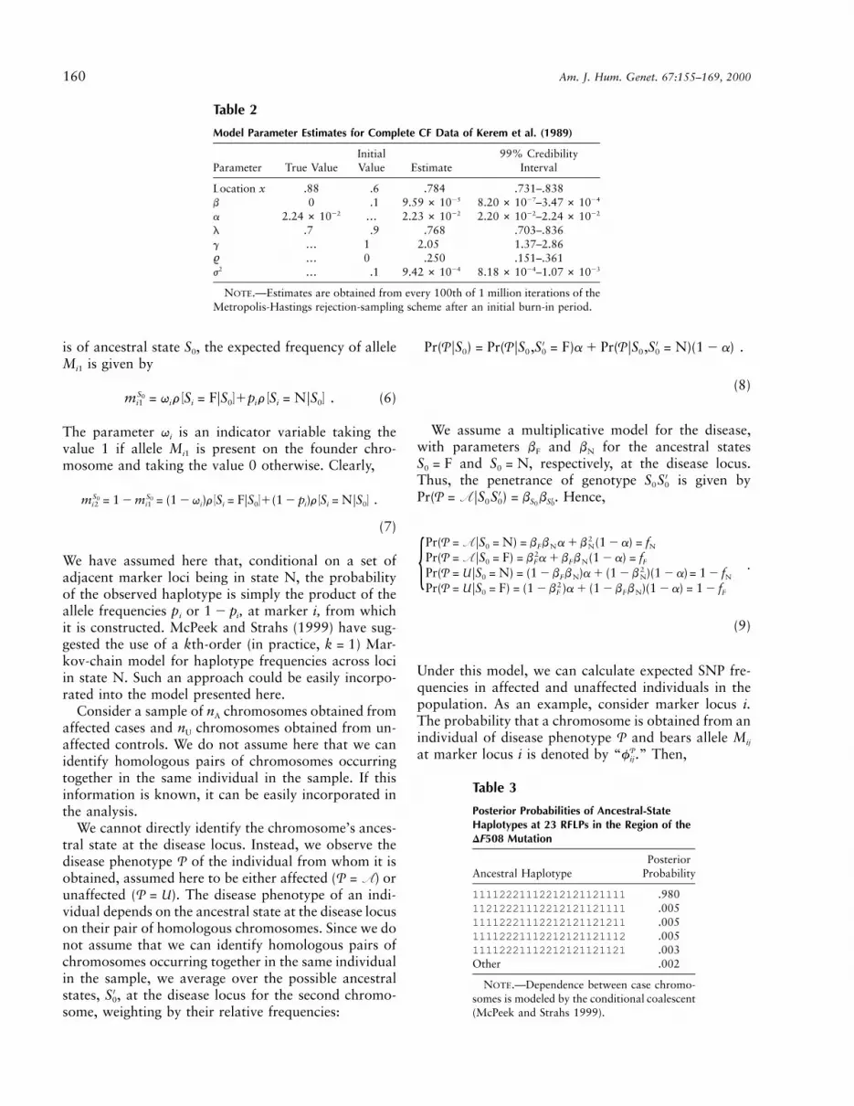
Model Parameter Estimates for Complete CF Data of Kerem et al. (1989)

Parameter True ValueInitialValue Estimate

99% CredibilityInterval

Location x .88 .6 .784 .731–.838b 0 .1 259.59 # 10 –27 248.20 # 10 3.47 # 10a 222.24 # 10 … 222.23 # 10 –22 222.20 # 10 2.24 # 10l .7 .9 .768 .703–.836g … 1 2.05 1.37–2.86% … 0 .250 .151–.361

2j … .1 249.42 # 10 –24 238.18 # 10 1.07 # 10

NOTE.—Estimates are obtained from every 100th of 1 million iterations of theMetropolis-Hastings rejection-sampling scheme after an initial burn-in period.

Table 3

Posterior Probabilities of Ancestral-StateHaplotypes at 23 RFLPs in the Region of the

MutationDF508

Ancestral HaplotypePosterior

Probability

11112221112212121121111 .98011212221112212121121111 .00511112221112212121121211 .00511112221112212121121112 .00511112221112212121121121 .003Other .002

NOTE.—Dependence between case chromo-somes is modeled by the conditional coalescent(McPeek and Strahs 1999).

is of ancestral state S0, the expected frequency of alleleMi1 is given by

S0 [ ] [ ]m = q r S = FFS 1p r S = NFS . (6)i1 i i 0 i i 0

The parameter qi is an indicator variable taking thevalue 1 if allele Mi1 is present on the founder chro-mosome and taking the value 0 otherwise. Clearly,

S S0 0 [ ] [ ]m = 1 2 m = (1 2 q )r S = FFS 1(1 2 p )r S = NFS .i2 i1 i i 0 i i 0

(7)

We have assumed here that, conditional on a set ofadjacent marker loci being in state N, the probabilityof the observed haplotype is simply the product of theallele frequencies pi or , at marker i, from which1 2 pi

it is constructed. McPeek and Strahs (1999) have sug-gested the use of a kth-order (in practice, ) Mar-k = 1kov-chain model for haplotype frequencies across lociin state N. Such an approach could be easily incorpo-rated into the model presented here.

Consider a sample of nA chromosomes obtained fromaffected cases and nU chromosomes obtained from un-affected controls. We do not assume here that we canidentify homologous pairs of chromosomes occurringtogether in the same individual in the sample. If thisinformation is known, it can be easily incorporated inthe analysis.

We cannot directly identify the chromosome’s ances-tral state at the disease locus. Instead, we observe thedisease phenotype of the individual from whom it isP

obtained, assumed here to be either affected ( ) orP = Aunaffected ( ). The disease phenotype of an indi-P = U

vidual depends on the ancestral state at the disease locuson their pair of homologous chromosomes. Since we donot assume that we can identify homologous pairs ofchromosomes occurring together in the same individualin the sample, we average over the possible ancestralstates, , at the disease locus for the second chromo-′S0

some, weighting by their relative frequencies:

′ ′Pr(PFS ) = Pr(PFS ,S = F)a 1 Pr(PFS ,S = N)(1 2 a) .0 0 0 0 0

(8)

We assume a multiplicative model for the disease,with parameters bF and bN for the ancestral states

and , respectively, at the disease locus.S = F S = N0 0

Thus, the penetrance of genotype is given by′S S0 0

. Hence,′Pr(P = AFS S ) = b b ′0 0 S S0 0

2Pr(P = AFS = N) = b b a 1 b (1 2 a) = f0 F N N N2Pr(P = AFS = F) = b a 1 b b (1 2 a) = f0 F F N F .2Pr(P = UFS = N) = (1 2 b b )a 1 (1 2 b )(1 2 a)= 1 2 f0 F N N N{

2Pr(P = UFS = F) = (1 2 b )a 1 (1 2 b b )(1 2 a) = 1 2 f0 F F N F

(9)

Under this model, we can calculate expected SNP fre-quencies in affected and unaffected individuals in thepopulation. As an example, consider marker locus i.The probability that a chromosome is obtained from anindividual of disease phenotype and bears allele MijP

at marker locus i is denoted by “ .” Then,Pfij


Table 4

Model Parameter Estimates for HD Data of MacDonald et al. (1991)

ParameterTrueValue

InitialValue Estimate

99% CredibilityInterval

Location x 2.5–2.6 2.2 2.52 2.20–2.75b 10 .1 232.08 # 10 –23 231.84 # 10 2.28 # 10a … … 231.09 # 10 –24 238.87 # 10 1.32 # 10l … .9 .854 .564–.998g … 1 1.37 .772–2.06% … 0 .111 .024–.177

2j … .1 296.88 # 10 –29 286.00 # 10 7.60 # 10

NOTE.—See Note to table 3.

Pf = Pr(P ∩ M )ij ij

= Pr(P ∩ M FS = F)a 1 Pr(P ∩ M FS = N)(1 2 a)ij 0 ij 0

F N= Pr(PFS = F)m a 1 Pr(PFS = N)m (1 2 a) ,0 ij 0 ij

(10)

since disease status and SNP type are independent, con-ditional on the chromosome’s ancestral state at the dis-ease locus. Thus, when we substitute for the appropriate

from equation (9) and for from equationsS0Pr(PFS ) m0 ij

(6) and (7),

A F Nf = m f a 1 m f (1 2 a) ,i1 i1 F i1 N

A F Nf = m f a 1 m f (1 2 a) ,i2 i2 F i2 N

U F Nf = m (1 2 f )a 1 m (1 2 f )(1 2 a) ,i1 i1 F i1 N

U F Nf = m (1 2 f )a 1 m (1 2 f )(1 2 a) .i2 i2 F i2 N

In a case-control study, affected individuals are ascer-tained with greater probability than is their populationfrequency, so that a sample will be enriched with casechromosomes. We denote by the observed frequen-Pnij

cies of allele Mij in the sample of chromosomes obtainedfrom individuals of disease phenotype . Table 1 pre-P

sents the expected case-control frequencies of SNP al-leles at marker locus i. The parameter Q is the popu-lation frequency of the disease, which is assumed to beknown, and k is a sample-enrichment factor: k =

. The expected frequencies are scaled{[(1 2 Q)n ]/Qn }A U

by the parameter to sum to 1.T = 1 1 Q(k 2 1)

Allowing for Mutations at Marker Loci

In deriving the model thus far, we have assumed thatno mutations at marker loci have occurred since thefounding disease mutation on the ancestral chromo-some. The method is designed for use with SNPs, whichare thought to have low mutation rates in humans,∼1028–1029/locus/generation (Nielsen 2000). For recentdisease mutations, the effects of such a low rate of mu-

tation will be negligible. Nevertheless, we may wish forthe model to account for marker mutation.

Under the assumption of no marker mutation, we ob-serve, at that locus, only the ancestral allele at markeri on a chromosome IBD with the founder. However, ifwe allow for marker mutation, we may observe the non-ancestral allele at a locus in state F. In terms of theindicator parameter for marker i,

100g(1 2 m) if allele M present on founder chromosomei1 ,100g{1 2 (1 2 m) otherwise

where m is the mutation rate per locus per generationand 100g is the number of generations since the found-ing mutation.

Allowing for Phenocopies

The model described has assumed, thus far, that allmutant chromosomes have descended from a single an-cestral founder. This assumption is unlikely to be realisticfor most human diseases (Penisi 1998). Phenocopies mayoccur either as a result of multiple mutations in the samegene or, especially for complex diseases, as a result ofthe effects of multiple susceptibility loci and the envi-ronment. In this section, we develop the model to allowfor phenocopies, under the assumption that there is asingle major mutation that accounts for a substantialproportion of affected individuals in the current gen-eration. This is true, for example, of CF, for which themajor DF508 mutation in the CFTR gene accounts foralmost 70% of all chromosomes in affected individuals,with many other mutations in the same gene accountingfor the remaining 30% (Kerem et al. 1989). Previousapproaches, with the exception of that of McPeek andStrahs (1999), fail to explicitly allow for this in theirassociation models.

Assume that the major mutation (F) accounts for aproportion l of all mutant chromosomes in the currentgeneration and that the major mutation and all othermutations ( ) have the same penetrance, bF. If equation

—F

162 Am. J. Hum. Genet. 67:155–169, 2000

(8) is generalized to allow for three possible ancestralstates,

′Pr(P = AFS ) = Pr(P = AFS ,S = F)al0 0 0

—′1Pr(P = AFS ,S = F)a(1 2 l)0 0

′1Pr(P = AFS ,S = N)(1 2 a) .0 0

Hence, as defined in equation (9),

Pr(P = AFS = N) = f0 N — . (11){Pr(P = AFS = F) = Pr(P = AFS = F) = f0 0 F

Then, in the same way as for equation (10),

——P F Ff = Pr(PFS = F)m al 1 Pr(PFS = F)m a(1 2 l)ij 0 ij 0 ij

N1Pr(PFS = N)m (1 2 a) ,0 ij

where the appropriate is obtained from equa-Pr(PFS )0

tion (11). However, since the phenocopies may be spu-rious or will have descended from many different an-cestral founding chromosomes, we assume that, in termsof the occurrence of marker alleles, they are indistin-guishable from any chromosome not bearing the majormutation at the disease locus; in other words,

—Fm =ij

as defined in equations (6) and (7).Nmij

Likelihood Calculations

Expected SNP allele frequencies to the left and rightof the disease locus are determined by independent Mar-kov processes. Thus, over the whole candidate region,the log-likelihood of a sample of data for a fixed locationof the disease gene, x, and a given set of hidden Mar-kov–model parameters is given by

ø(dataFx,G,p,w) = ø(dataFx,G,p,w) 1 ø(dataFx,G,p,w) ,TOT L R

where is a vector of model parameters,G G =, and and are vectors of allele fre-T(a,b ,b ,g,l) p wF N

quencies and ancestral indicators, respectively:

Tp = (p ,p ,...,p ,p ,p ,p ,...,p ,p ) ,2L 2(L21) 22 21 1 2 R21 R

and

Tq = (q ,q ,...,q ,q ,q q ,...,q ,q ) .2L 2(L21) 22 21 1 2 R21 R

The log-likelihood to the right of the disease locus isgiven by

R 2 U

P P[ ]ø(dataFx,G,p,w) = n ln f 1C ,OOOR ij ij Ri=1 j=1 P=A

where CR is constant for a known population diseasefrequency Q: . The indepen-C = Rkn 2 RT (n 1 n )R A A U

dent log-likelihood to the left of the disease locus is cal-culated similarly.

Parameter Estimation

The hidden Markov model described here is overpa-rameterized. We reduce the number of free parametersby noticing the following relationships.

First, the population frequency of the disease is givenby

2 2 2 2Q = a b 1 2a(1 2 a)b b 1 (1 2 a) b .F F N N

The frequency of the disease is generally known so thatwe can eliminate a from the likelihood calculation:

2 2 2 2Î22b (b 2 b ) 5 4b (b 2 b ) 2 4(b 2 b ) (b 2 Q)N F N N F N F N Na =

22(b 2 b )F N

ÎQ 2 bN= ,

b 2 bF N

since .a 1 0Second, the likelihood is constant for a fixed ratio of

disease-model parameters . Thus, the two pa-b = b /bN F

rameters can be eliminated from the likelihood and canbe replaced by a single penetrance parameter for which

, since it is assumed that, at the disease locus, theb < 1mutation has greater propensity for the development ofthe disease than does the normal allele. Overall, for aknown disease frequency Q, the vector of model param-eters to be estimated reduces to , togetherTG = (b,g,l)with the allele frequencies and ancestral indicators.

We use MCMC methods to obtain posterior distri-butions for the model parameter estimates. The advan-tage of this approach is that we can incorporate priorinformation for the model parameters—which may beuseful if we have reliable values for the age of the mu-tation or disease model, for example. We employ a Me-tropolis-Hastings algorithm (Metropolis et al. 1953;Hastings 1970) to obtain realizations of each model pa-rameter by sampling from the full conditional distri-bution, using a rejection-sampling scheme. Each itera-tion of the sampling scheme consists of a six-stepprocedure summarized in Appendix B. From initial pa-rameter values, the algorithm is run for a substantialburn-in period, to allow convergence. During the sub-sequent sampling period, realizations of the parameterset are recorded every 100th iteration. Over many it-erations, posterior distributions of parameter estimatesare obtained from these realizations.


Allowing for Heterogeneity in Recombination Rates

In developing the hidden Markov model for fine-scalemapping, we have assumed a constant ratio of recom-bination fraction to physical distance across the wholeof the candidate region. However, it is thought that re-combination hot spots and cold spots occur along thegenome. Lazzeroni (1998) accounts for heterogeneity inrecombination rates in a generalized least-squares ap-proach to fine-scale mapping, by allowing the ratio ofphysical distance to genetic distance to be different tothe left and to the right of the disease locus. However,this may not be sufficient to allow for the variability inrecombination rates, particularly in larger candidateregions.

As an alternative, we propose that the ratio of physicaldistance to genetic distance across the candidate regioncan be described by a first-order Gaussian autoregressiveprocess. We divide the candidate region into K equalintervals so that the rate of recombination, yr, in the rthinterval is given by and∗y = m 1 e y = m 1 %(y 21 1 r r21

, where m is the mean recombination rate acrossm) 1 er

the region and % is the first-order correlation coefficient.The errors are assumed to be independently distributed,so that and for∗ 2 2 2e ∼ N(0,j /(1 2 %) ) e ∼ N(0,j ) r =1 r

. The log-likelihood of a sample of K recombi-2,3,...,Knation rates from this process is then given by

K2 2 2ø(yFm,%,j ) = 2 ln (2pj ) 1 ln (1 2 % )AR1 22 2(y 2 m) (1 2 % )12 2j

K1 2[ ]2 (y 2 m) 2 %(y 2 m) .O r r212j r=2

We assume that m is known from existing physical andgenetic maps. Uncertainty for this parameter can be in-corporated by assuming a tight prior distribution for m,centered about the estimated ratio. For example, in theregion of the CFTR gene for CF, a physical distance of1.6 Mb corresponds to a genetic distance of ∼0.8 cM(Collins et al. 1996)—in other words, .m = .5

The recombination rates across the region can thenbe used in calculating the probability of no recombi-nation events in the interval between any pair of adja-cent marker loci; for example, the probability of no re-combination events in the interval between marker i and

is given by , wherei 1 1 exp [2gd v ] v =i11 i11 i11

and pr denotes the proportion of the rthK KS y p /S pr=1 r r r=1 r

recombination-rate interval contained in the interval be-tween the two marker loci. The log-likelihood of thesample of data for a given set of recombination rates

and hidden Markov–model parameters is expressed byy

. The recombination rates are, in ef-ø(dataFx,G,p,w,y)TOT

fect, nuisance parameters, so that

2ø(dataFx,G,p,w) = ø(dataFx,G,p,w,y) ø(yFm,%,j ) .TOT E TOT AR1y

In this way, we can then incorporate heterogeneous re-combination rates into the Metropolis-Hastings rejec-tion-sampling scheme for the model parameters as de-scribed in Appendix B.

Allowing for Nonindependent RecombinationalHistories

In developing the hidden Markov model for disease-marker association in the region of a disease gene, wehave assumed independent recombinational histories foreach chromosome in the sample. However, the key tothis approach to disease-gene mapping is that all—or atleast a majority of—affected individuals share a recentsingle common ancestor bearing the disease-predispos-ing mutation. Treating the recombinational histories asindependent is equivalent to assessing a star-shaped ge-nealogy, which is not consistent with likely demographicscenarios for the development of a disease mutation ina finite population. Instead, we expect particular pairsof chromosomes to have a more recent common ances-tor than do other pairs of chromosomes—and, conse-quently, to share a greater proportion of their recom-binational history. The effect of this shared ancestry isto down-weight the contribution of each case chromo-some to the total log-likelihood by a factor [1 1 (n 2A

, where c is given by211)c]

21` n 1 i 2 1Ai21O (21) ( )n 22 [ ]A n 2 ki=1 A2(n 2 2)!(n 1 1)A A .O

n 2 1 (n 2 k 1 1)(n 2 k 1 2)(n 2 k)(k 2 1)!(n 2 k 2 2)!k=1A A A A A

Since the correction factor is !1, we effectively down-weight the contribution of each case chromosome to thetotal log-likelihood, to account for the dependence be-tween them. We emphasize here that a quasi-likelihoodapproach is not applicable in a Bayesian framework; butit does suggest the use of a likelihood approximation.We propose to multiply the log-likelihood calculated un-der a star-shaped genealogy by the same correction fac-tor. This has the effect of increasing the variance of theposterior distribution, to account for the shared ancestryof the case chromosomes.

Examples

To illustrate our proposed method, we consider two dis-eases: CF and HD. Mutations responsible for the oc-currence of these two diseases have been located on the

164 Am. J. Hum. Genet. 67:155–169, 2000

genome and are thus ideal for testing the accuracy andprecision of the new method. In this section, we applythe proposed method to marker-haplotype data collectedin candidate regions for the two disease genes (Keremet al. 1989; MacDonald et al. 1991). In both samples,cases and controls have been typed by RFLPs. Since thesemarkers have low rates of mutation, we have assumedthat , corresponding to no marker mutation in them = 0period since the founding disease mutation.

CF

CF is one of the most common autosomal recessivedisorders affecting whites, occurring with an incidenceof 1 case/2,000 births. Initial scans of the genome in the1980s provided evidence of a single CF gene on chro-mosome 7q31 (Kerem et al. 1989). More recently, a 3-bp deletion (DF508) has been identified within this re-gion in the CFTR gene. It is now known that DF508accounts for ∼68% of all chromosomes in affected in-dividuals today, with the remainder consisting of severalother, rarer mutations in the same gene. Kerem et al.(1989) collected marker data from affected cases andhealthy controls, using 23 RFLPs in a 1.8-Mb candidateregion of chromosome 7q31, from the MET locus tomarker D7S426.

Figure 1 presents odds ratios for each of the RFLPsin the candidate region. There is strongest evidence ofdisease-marker association in a region of 0.6–0.9 Mbfrom the MET locus, with a peak observed at 0.869 Mb.Within this region, however, there is a single marker,0.889 Mb from the MET locus, at which disease-markerassociation is much lower. This marker is, in fact, closestto the DF508 mutation in the CFTR gene, at ∼0.880Mb from the MET locus.

Previous analyses of these data by published methodshave yielded a variety of results. Terwilliger (1995)places the mutation 0.77 Mb from the MET locus, witha 99.9% support interval of 0.69–0.87 Mb. Althoughthis interval overlaps part of the CFTR gene, it does notinclude the DF508 mutation. Xiong and Guo (1997)obtained an improved estimate of the location of DF508,at 0.80 Mb, although this was derived from only a se-lected subset of the CF data, a subset for which any casechromosomes not bearing the DF508 mutation were ex-cluded. With additional information for the region ofthe mutation (Morral et al. 1994), Collins and Morton(1998) analyzed the same subset and obtained an esti-mate of 0.83 Mb.

We applied the hidden Markov model–based mappingmethod proposed here to the complete CF data set ofKerem et al. (1989). We assumed a disease frequency of

, on the basis of estimates for the populationQ = .0005from which the sample was ascertained. We also as-sumed a mean recombination rate of .5, since, in the

candidate region around the CFTR gene, the physicaldistance of 1.6 Mb corresponds to a genetic distance of0.8 cM (Collins et al. 1996). A number of sets of initialvalues for the model parameters were considered, allresulting in similar posterior distributions and parameterestimates after an initial burn-in period of the Metrop-olis-Hastings rejection-sampling scheme followed by asampling period of a further 1 million iterations forwhich every 100th iteration was recorded. Regardless ofthe starting values for the model parameters, there israpid convergence to parameter estimates, which alsoappear to mix well (data not shown).

Figure 2 presents the posterior distributions of thelocation of the mutation, the hidden Markov–model pa-rameters b, a, l, and g, and the first-order autoregressiveparameters % and for recombination-rate heteroge-2j

neity across the candidate region, when independent re-combinational histories for the case and control chro-mosomes are assumed. Also presented is the distributionof the hidden Markov–model log-likelihood obtainedthroughout the sampling period. Table 2 presents theinitial parameter values for this run, together with thetrue parameter values (where known) and summary sta-tistics from the posterior distributions.

The mean estimate of the location of the mutation isMb from the MET locus, with a 99% credi-x = 0.784

bility interval of 0.731–0.838 Mb. Although there issubstantial error in this estimate, the results are consis-tent with estimates obtained by other case-control–basedmapping methods, which have been described above.The frequency of the mutation is estimated as a =

. This is in agreement with a mutation-frequency.223estimate of .224 based on a fully penetrant recessivedisease with frequency .0005 (Kerem et al. 1989). Theestimate of the disease-model parameter approachesb

0, which is as would be expected for a fully penetrantrecessive disease for which and . The esti-b = 1 b = 0F N

mated major-mutation proportion is , which isl = .768close to the estimate that 70% of existing CF chromo-somes bear the DF508 mutation. The estimated age ofthe mutation is , corresponding to 205 gener-g = 2.05ations. Again, this is not inconsistent with other, inde-pendent estimates of the age of DF508, which suggestthat it is ∼200 generations old (Serre et al. 1990). Cred-ibility intervals for the first-order autoregressive param-eters do not include 0, suggesting that there is recom-bination-rate heterogeneity across the candidate region.

For comparison, we have also applied the hidden Mar-kov model–based mapping method to the same set ofdata but have modeled dependence between case chro-mosomes by using the conditional coalescent as pro-posed by McPeek and Strahs (1999). Figure 3 presentsthe posterior distribution of the model parameters thatis based on every 100th of 1 million iterations of theMetropolis-Hastings rejection-sampling scheme, with


the log-likelihood being corrected for between-chro-mosome correlations.

We obtain an improved estimate of the location ofDF508: 0.798 Mb from the MET locus, with a 99%credibility interval of 0.610–1.069 Mb, this time withthe true location of the mutation being included. Theother model parameter estimates remain relatively un-changed, but with noticeably wider posterior credibilityintervals (data not shown). The exception is in the first-order autoregressive-process–correlation parameter, themean estimate of which is considerably closer to 0 underthe coalescent model (.053) than under independence(.250). This would suggest that much of the correlationbetween marker loci is accounted for by the correlationbetween related chromosomes.

With the same correction, McPeek and Strahs (1999)estimate the location of the mutation to be 0.95 Mbfrom the MET locus, with a 99% confidence interval of0.28–1.62 Mb (calculated on the basis of their presented95% confidence interval). The difference, in estimatedlocation, between the two methods is likely a result ofMcPeek and Strahs’s (1999) assumption of a homoge-neous recombination rate of 1 cM–1 Mb across the mapof marker loci.

Table 3 presents the posterior ancestral-haplotypesprobabilities realized over the 1 million iterations of theMetropolis-Hastings rejection-sampling scheme. Thereis complete agreement over all but the markers mostdistant from the DF508 mutation at which levels of dis-ease-marker association are weakest. For this particularsample, maximizing the model likelihood over the an-cestral haplotype, as in the method of McPeek and Strahs(1999), would be expected to yield results similar tothose of our proposed method, since the maximum-like-lihood estimate has such high posterior probability. Withless certainty with regard to ancestral haplotypes, max-imum-likelihood–based approaches may suffer bias andwarrant further investigation.

HD

HD is a midlife-onset autosomal dominant neurode-generative disorder occurring at an incidence of ∼1 case/10,000. The HD gene was first mapped to chromosome4p16, in the region of marker D4S10, by Gusella et al.(1983, 1984). More recently, the Huntington’s DiseaseCollaborative Research Group (1993) has identifiedwithin this region a large gene (IT15) with an expand-able unstable trinucleotide-repeat sequence. It is nowknown that IT15 genes with many repeats of the tri-nucleotide sequence are responsible for the developmentof the disease. MacDonald et al. (1991) collected markerdata from HD and normal chromosomes in a 2.5-Mbregion of chromosome 4p16, from marker D4S90 toD4S10, using 27 RFLPs.

Figure 4 presents odds ratios for each of the RFLPsin the candidate region. The strongest evidence of dis-ease-marker association lies in the interval betweenmarkers D4S182 and D4S180, at 2.38 Mb and 2.85 Mb,respectively, from marker D4S90. This is in agreementwith the location of IT15 at ∼2.5–2.6 Mb from markerD4S90. As in the CF data of Kerem et al. (1989), thereare RFLPs with low levels of disease-marker associationwithin this interval. Despite this apparent inconsistency,Xiong and Guo (1997), using their case-control–basedmapping method, obtained 2.62 Mb from markerD4S90 as the estimated location of the disease gene.

We also have applied the hidden Markov model–basedmapping method to the HD data of MacDonald et al.(1991). We assumed independent recombinational his-tories for the case chromosomes and a disease frequencyof , in line with published estimates for pop-24Q = 10ulations of European descent. We also assumed a meanrecombination rate of 1 in the candidate region, so thatthe usual 1 Mb– to–1 cM correspondence holds. Weconsidered various sets of initial values for the modelparameters, all resulting in similar posterior distribu-tions and parameter estimates after the same burn-inperiod and sampling period that were employed in theanalysis of the CF data.

Figure 5 presents, for the HD data, the posterior dis-tributions for the hidden Markov model and autore-gressive parameters. Summary statistics from the pos-terior distributions of model parameters are presentedin table 4, together with true values (where known). Themean estimate of the location of the mutation is 2.52Mb from marker D4S90, with a 99% credibility intervalof 2.20–2.75 Mb. The mean estimate is accurate, beingcontained within the IT15 gene for HD. The wide cred-ibility interval reflects the considerable variation in thestrength of disease-marker association in the IT15 gene(fig. 4).

The estimate of the disease model parameter b =is 10, which we would expect for a dominant232.1 # 10

disease. The estimated age of the mutation is ,g = 1.37corresponding to 137 generations, and is not inconsis-tent with other estimates of the age of HD (Kaplan etal. 1995; Xiong and Guo 1997). Credibility intervals forthe autoregressive parameters do not include 0, sug-gesting recombination-rate heterogeneity across the can-didate region.

Discussion

We have presented a new multilocus method for the fine-scale mapping of disease genes. We model disease-marker association in the vicinity of a disease gene bymeans of a hidden Markov process used in a way similarto that employed by McPeek and Strahs (1999). In thisway, both models account for correlation between the

166 Am. J. Hum. Genet. 67:155–169, 2000

markers, a clear advantage over many existing multilo-cus composite-likelihood methods that assume inde-pendence (Terwilliger 1995; Xiong and Guo 1997; Col-lins and Morton 1998). In addition, both models allowfor mutation at marker loci.

We employ MCMC methods in a Bayesian frame-work, to obtain posterior distributions for model pa-rameter estimates including those for disease-gene lo-cation and the age of the disease-predisposing mutation.A potential advantage of this approach, over both themaximum-likelihood estimation used by McPeek andStrahs (1999) and other existing multipoint methods, isthat, where appropriate, we are able to incorporateprior information for model parameters. In addition, byintegrating over the marker haplotype present on thefounding chromosome, we allow for the uncertainty inits makeup, in contrast to McPeek and Strahs (1999),who consider only the maximum-likelihood estimate.

Our model is more sophisticated than previous mod-els in that we allow for recombination-rate heteroge-neity across the candidate region, using a first-orderGaussian autoregressive process. In this way, we canallow for recombination hot spots and cold spots thatmay lead to bias in existing models. However, it wouldbe relatively straightforward to incorporate variable re-combination rates in the model proposed by McPeekand Strahs (1999).

We have used our method to identify the location oftwo known mutations—one for CF and one for HD.For HD, we obtain an accurate estimate of the locationof the mutation within the IT15 gene, which is knownto be responsible for the development of the disorder.In deriving the hidden Markov model for disease-marker association, we have assumed a multiplicativemodel for the disease. HD is a dominant (i.e., non-multiplicative) disorder, suggesting that our method isrobust to deviations from a multiplicative-diseasemodel.

For CF, we have presented two sets of simulationresults, corresponding to two possible models of de-pendence in the recombinational histories of chromo-somes in affected individuals. First, we have assumedindependence, implying a star-shaped genealogy, whichyields, for the location of the mutation, a 99% credi-bility interval that does not contain the true location ofDF508. This result is consistent with analyses of thesame data set by other multilocus models that assumeindependence between case chromosomes (Terwilliger1995; Xiong and Guo 1997; Collins and Morton 1998).

This clearly suggests deficiency in the star-shaped ge-nealogical model of case-chromosome ancestry. For thesecond set of simulations, we correct for correlationbetween case chromosomes by means of a conditionalcoalescent model of dependence, proposed by McPeekand Strahs (1999). They justify the correction by meansof quasi-likelihood arguments (Wedderburn 1974) thatdo not hold in a Bayesian framework. However, thesame arguments suggest the use of an approximate log-likelihood, calculated by multiplication, by a correctionfactor, of the log-likelihood under independent recom-binational histories (McPeek and Strahs 1999). This hasthe effect of increasing the variance of the posteriordistribution, to account for the shared ancestry of casechromosomes.

An alternative approach to take account of the de-pendence between chromosomes is to model their an-cestry directly, by means of a genealogical tree. In sucha model, we can explicitly allow for multiple diseasemutations, mutations at marker loci within the candi-date region, and recombination events in the ancestryof the case sample. Lam et al. (2000) have constructeda genealogical tree for case chromosomes by using acombination of parsimony and likelihood methods, inwhich each chromosome in the tree is separated fromits parent by a single marker mutation or recombinationevent. They then proceed to map the disease mutationas if the tree were known with certainty. A more ap-propriate approach would be to integrate over all pos-sible genealogies, an approach that can be approxi-mated by simulation. Graham and Thomson (1998)used such an approach to generate genealogical treesthat are consistent with an observed sample of chro-mosomes, using a Moran (1962) model with knowndemographic parameters. However, their model as-sumes knowledge of the ancestral marker haplotype, thenumber of generations since the common ancestor, andthe development of the population during this period.It is currently restricted to interval mapping using pairsof marker loci. Generalization of this approach to a fullmultilocus analysis with less stringent assumptions re-mains a challenge that will require considerable workin the future.

Acknowledgments

A.P.M. acknowledges financial support from Pfizer Limited.We thank the referees for their helpful comments on the sub-mitted version of this article.


Appendix A

Summary of Model Parameters

Parameter Range Definitiona [0,1] Probability that chromosome is IBD with founder, at any given locusbF [0,1] Disease model parameter associated with mutation at disease locusbN [0,1] Disease model parameter associated with normal allele at disease locusg [0,`] Recombination-rate parameter per 1 Mb of DNA in candidate regionpi [0,1] Frequency of allele Mi1 on chromosomes not IBD with founder, at locus iqi 0 or 1 Indicator variable denoting presence/absence of allele Mi1Q [0,1] Population frequency of diseasek [0,`] Sample-enrichment factor

Appendix B

Metropolis-Hastings Rejection-Sampling Scheme

Each iteration of the Metropolis-Hastings samplingscheme consists of a seven-step procedure. We denotethe current parameter set by x, , , and . In addition,G p wthe current set of recombination rates is denoted , mod-yeled as a first-order autoregressive process with knownmean recombination rate m and current parameters %and . If we do not wish to allow for heterogeneity in2j

recombination rates across the candidate region, y = 1and we ignore step 7 of the sampling scheme. The like-lihood of a sample of cases and controls for the currentparameter set is denoted . The like-L(dataFx,G,p,w,y)TOT

lihood of the set of recombination rates for the currentparameter set is denoted . Throughout, we2L(yFm,%,j )AR1

assume each « to be drawn at random from the proposaldistribution U(2.5,.5) and each u to be drawn fromU(0,1).1. For each marker j in turn, propose a new allelefrequency, , where determines the maxi-∗p = p 1 n « nj j p p

mum possible change from the current allele frequency.Since , proposed allele frequencies outside thisp P [0,1]j

range are reflected back into the parameter space. Thelikelihood for the proposed parameter set is denoted

where is the vector of currentj∗ j∗L(dataFx,G,p ,w,y) pTOT

allele frequencies with replaced by the proposed .∗p pj j

The proposed allele frequency is accepted to the currentparameter set if the acceptance probability is

j∗L(data F x,G,p ,w,y)TOTa = min ,1 1 u .[ ]L(data F x,G,p,w,y)TOT

2. For each marker j, in turn, propose a new ancestralindicator:

0 if « < 0∗q = .j {1 if « 1 0

The likelihood for the proposed parameter set is denotedwhere is the vector of currentj∗ j∗L(dataFx,G,p,w ,y) wTOT

ancestral indicators with replaced by the proposedqj

. We then accept the proposed ancestral indicator to∗qj

the current parameter set if the acceptance probabilityis

j∗L(dataFx,G,p,w ,y)TOTa = min ,1 1 u .[ ]L(dataFx,G,p,w,y)TOT

3. Propose a new location for the disease gene, ∗x =, where the parameter determines the maximumx 1 n « nx x

change from the current disease gene location. We re-strict the location of the disease gene to the candidateregion, so that proposed locations distal to the first andlast markers on the map are reflected back into the can-didate region. The likelihood for the proposed parameterset is denoted and the proposed∗L(dataFx ,G,p,w,y)TOT

location is accepted to the current parameter set if

∗L(dataFx ,G,p,w,y)TOTa = min ,1 1 u .[ ]L(dataFx,G,p,w,y)TOT

4. Propose a new penetrance parameter, ,∗b = b 1 n «b

where determines the maximum change from the cur-nb

rent penetrance parameter. The penetrance parameter isrestricted to so that proposed penetrances out-b P [0,1]side this range are reflected back into the parameterspace. The likelihood for the proposed parameter set isdenoted where is the vectorb∗ b∗L(dataFx,G ,p,w,y) GTOT

of current hidden Markov–model parameters with b re-

168 Am. J. Hum. Genet. 67:155–169, 2000

placed by the proposed . The proposed penetrance∗b

parameter is then accepted to the current parameter setif the acceptance probability is

b∗L(dataFx,G ,p,w,y)TOTa = min ,1 1 u .[ ]L(dataFx,G,p,w,y)TOT

5. Propose a new age of the mutation, ,∗g = g 1 n «g

where determines the maximum change from the cur-ngrent age of the mutation. The age of the mutation isrestricted to be positive so that a negative proposed ageis reflected back into the valid parameter space. Thelikelihood for the proposed parameter set is denoted

, where is the vector of currentg∗ g∗L(dataFx,G ,p,w,y) GTOT

hidden Markov–model parameters with g replaced bythe proposed . The proposed age of the mutation is∗g

then accepted to the current parameter set if the accep-tance probability is

g∗L(dataFx,G ,p,w,y)TOTa = min ,1 1 u .[ ]L(dataFx,G,p,w,y)TOT

6. Propose a new major mutation proportion, ∗l =, where determines the maximum change froml 1 n « nl l

the current proportion. Since l is a proportion, it isrestricted to [0,1]. Proposed proportions outside thisrange are reflected back into the valid parameter space.The likelihood for the proposed parameter set is denoted

, where is the vector of currentl∗ l∗L(dataFx,G ,p,w,y) GTOT

hidden Markov–model parameters with l replaced bythe proposed . The proposed major mutation propor-∗l

tion is then accepted to the current parameter set if theacceptance probability is

l∗L(dataFx,G ,p,w,y)TOTa = min ,1 1 u .[ ]L(dataFx,G,p,w,y)TOT

7. Propose a new set of K recombination rates so that,for each , , where determines∗i = 1,2,...,K y = y 1 n « ni i y y

the maximum change from the current recombinationrates. Each recombination rate is restricted to be non-negative so that negative proposals are reflected backinto the valid parameter space. In the same step, we alsopropose new autoregressive parameter values, ∗% =

and , where and determine the∗ ∗% 1 n « j = j 1 n « n n% j % j

maximum change in parameter values for % and j, re-spectively. The correlation parameter and the% P [0,1]standard deviation j is restricted to be positive. Pro-posals outside the permitted space are reflected back tovalid parameter values. The likelihoods for the proposedparameters and recombination rates are denoted

and . The com-∗ ∗ ∗2 ∗L(y Fm,% ,j ) L(dataFx,G,p,w,y )AR1 TOT

plete set of proposed recombination rates and autore-gressive parameters are accepted to the current set if

∗ ∗ ∗ ∗2L(dataFx,G,p,w,y ) L(y Fm,% ,j )TOT AR1a = min ,1 1 u .2[ ]L(dataFx,G,p,w,y) L(yFm,%,j )TOT AR1

At any stage we can incorporate prior distributions formodel parameters by multiplying the appropriate accep-tance probability by the ratio of prior probabilities forthe proposed and current parameter values.

References

Collins A, Frezal J, Teague J, Morton NE (1996) A metric mapof humans: 23,500 loci in 850 bands. Proc Natl Acad SciUSA 93:14771–14775

Collins A, Morton NE (1998) Mapping a disease locus byallelic association. Proc Natl Acad Sci USA 95:1741–1745

Graham J, Thompson EA (1998) Disequilibrium likelihoodsfor fine-scale mapping of a rare allele. Am J Hum Genet 63:1517–1530

Gusella JF, Tanzi RE, Anderson MA, Hobbs W, Gibbons K,Raschtchian R, Gilham TC, et al (1984) DNA markers fornervous system disorders. Science 225:1320–1326

Gusella JF, Wexler NS, Conneally PM, Naylor SL, AndersonMA, Tanzi RE, Watkins PC, et al (1983) A polymorphicDNA marker genetically linked to Huntington’s disease. Na-ture 306:234–208

Hastings WK (1970) Monte-Carlo sampling methods us-ing Markov chains and their applications. Biometrika 57:97–109

Huntington’s Disease Collaborative Research Group (1993) Anovel gene containing a tri-nucleotide repeat that is ex-panded and unstable on Huntington’s disease chromosomes.Cell 72:971–983

Kaplan NL, Hill WG, Weir BS (1995) Likelihood methods forlocating disease genes in nonequilibrium populations. Am JHum Genet 56:18–32

Kerem B, Rommens JM, Buchanan JA, Markiewicz D, CoxTK, Chakravarti A, Buchwald M, et al (1989) Identificationof the cystic fibrosis gene: genetic analysis. Science 245:1073–1080

Kruglyak L (1999) Prospects for whole-genome linkage dise-quilibrium mapping of complex disease genes. Nat Genet22:139–145

Lam JC, Roeder K, Devlin B (2000) Haplotype fine mappingby evolutionary trees. Am J Hum Genet 66:659–673

Lander ES, Green P (1987) Construction of multi-locus geneticmaps in humans. Proc Natl Acad Sci USA 84:2363–2367

Lazzeroni LC (1998) Linkage disequilibrium and gene map-ping: an empirical least squares approach. Am J Hum Genet62:159–170

MacDonald ME, Lin C, Srinidhi L, Bates G, Altherr M,Whaley WL, Lehrach H, et al (1991) Complex patterns oflinkage disequilibrium in the Huntington’s disease region.Am J Hum Genet 49:723–734

McPeek MS, Strahs A (1999) Assessment of linkage disequi-


librium by the decay of haplotype sharing, with applicationto fine scale genetic mapping. Am J Hum Genet 65:858–875

Metropolis N, Rosenbluth AW, Rosenbluth MN, Teller AH,Teller E (1953) Equation of state calculations by fast com-puting machines. J Chem Phys 21:1087–1092

Moran P (1962) The statistical processes of evolutionary the-ory. Clarendon Press, Oxford

Morral N, Bertranpetit J, Estevill X, Nunes V, Casals T, Gi-menez J, Reis A, et al (1994) The origin of the major cysticfibrosis mutation (delta-F508) in European populations. NatGenet 7:169–175

Nielsen R (2000) Estimation of population parameters andrecombination rates from single nucleotide polymorphisms.Genetics 154:931–942

Ott J (1991) Analysis of human genetic linkage. John HopkinsUniversity Press, Baltimore

Penisi E (1998) A closer look at SNPs suggests difficulties.Science 281:1787–1789

Rabiner LR (1989) A tutorial on hidden Markov models and

selected applications in speech recognition. Proc IEEE 77:257–286

Risch N, Merikangas K (1996) The future of genetic studiesof complex human diseases. Science 273:1516–1517

Serre JL, Simon-Bouy B, Morret E, Jaume-Roig B, Balasso-poulou A, Schwartz M, Taillander A (1990) Studies ofRFLPs closely linked to the cystic-fibrosis locus throughoutEurope lead to new considerations in population genetics.Hum Genet 84:449–454

Terwilliger J (1995) A powerful likelihood method for theanalysis of linkage disequilibrium between trait loci and oneor more polymorphic marker loci. Am J Hum Genet 56:777–787

Wedderburn RWM (1974) Quasi-likelihood functions, gen-eralized models, and the Gauss-Newton method. Biometrika61:439–447

Xiong M, Guo S-W (1997) Fine scale genetic mapping basedon linkage disequilibrium: theory and applications. Am JHum Genet 60:1513–1531

Documents

Bayesian Fine-Scale Mapping of Disease Loci, by Hidden Markov Models