Embed Size (px)
Citation preview
HAL Id: tel-01989048https://tel.archives-ouvertes.fr/tel-01989048
Submitted on 22 Jan 2019
HAL is a multi-disciplinary open accessarchive for the deposit and dissemination of sci-entific research documents, whether they are pub-lished or not. The documents may come fromteaching and research institutions in France orabroad, or from public or private research centers.
L’archive ouverte pluridisciplinaire HAL, estdestinée au dépôt et à la diffusion de documentsscientifiques de niveau recherche, publiés ou non,émanant des établissements d’enseignement et derecherche français ou étrangers, des laboratoirespublics ou privés.
Optimal control of linear complementarity systemsAlexandre Vieira
To cite this version:Alexandre Vieira. Optimal control of linear complementarity systems. Automatic Control Engineer-ing. Université Grenoble Alpes, 2018. English. NNT : 2018GREAT064. tel-01989048

THESEPour obtenir le grade de
DOCTEUR DE LACOMMUNAUTE UNIVERSITE GRENOBLEALPESSpecialite : Automatique-Productique
Arrete ministeriel : 25 mai 2016
Presentee par
Alexandre Vieira
These dirigee par Bernard Brogliatoet codirigee par Christophe Prieur
preparee au sein de l’Inria Grenoble Rhone-Alpesdans l’Ecole Doctorale EEATS
Commande optimale des systemesde complementarite lineaires
These soutenue publiquement le 25 septembre 2018,devant le jury compose de :
Eric BlayoProfesseur des Universites, Univ. Grenoble Alpes, PresidentPierre RiedingerProfesseur des Universites, Univ. de Lorraine, RapporteurEmmanuel TrelatProfesseur des Universites, Sorbonne Universite, CNRS, RapporteurKanat CamlibelAssociate Professor, University of Groningen, ExaminateurBernard BrogliatoDirecteur de Recherche Inria, Univ. Grenoble Alpes, Directeur de theseChristophe PrieurDirecteur de Recherche CNRS, Directeur de these

Thanks/Remerciements
I have to admit that when I started my PhD, I had already thought about this thanks part (it wasa goal for me, as much as the manuscript itself...). It looks like marble to me: the names writtenhere will last as long as there is a copy of this manuscript. So yes: it is going to be a bit long. Iwill write first in English, and then in Français, so that no one feels excluded. Also, sorry for therepetition of the words thank and merci : the exercice imposes it.
My first thoughts go of course to Bernard and Christophe, my two advisors. I must say: thankyou, from the bottom of my heart, for these three years. Thank you for your presence, for all themeetings we did, and for your persistence, even in the moments when I was making you confused(by the way: sorry for that, I hope I made that up!). Thank you also for granting me freedom inthe directions I decided to follow for this research. I admit that some moments were frustratingfor me, and I may have been a little stubborn, but I am happy to see that, eventually, we did ajob I am feeling proud of.
Talking about being proud, I would like to express my gratitude to the members of my jury,Messrs. Blayo, Camlibel, Riedinger and Trélat. It makes me proud, indeed, to know that my workis being reviewed by such a talented jury. Thank you for the time spent on this thesis, and foradding a taste of credibility to my work.
These three years would have been tasteless without all the people I have met here in Grenoble.I am thankful to all the researchers and permanent engineers of feu BIPOP, Florence (I am startingwith you to be gallant!), Arnaud, Franck, Guillaume, Jerôme, Pierre-Brice, Vincent; thanks for thediscussions we had, the interesting remarks or problems you gave me, which made me come outof my comfort zone to reach greater knowledge. A special thank you for my dear Diane: you havealways been the best! I thank all the non-permanent people, all the post-docs, the engineers, thePhD students, the interns that I have met: Camille, Diana, Mounia, Thoï, Alejandro, Dimitar,Éric, Felix, Gilles, Janusz, Hadi, Kirill, Mickaël, Matteo, Nahuel, Narendra, Nestor, Nicolas. Icould have written a thousand times Janusz, but that would not be fair. Thank you all for the teatimes, the cakes (I know, I should bring more of them), the games, the laughs, the restaurants, themovies, the (sometimes serious or technical) discussions... Thank you mates, for sharing a slice ofjoyful life with me. Also, I would blame myself for forgetting all the people I met on the way inthe different meetings and conferences I attended. Thank you for all the useful feedback you gaveme. A big thank you to Emilio: this week discussing about so many things in Padova was moreinspiring than you may think!
J’ai une pensée également pour mes collègues de la prépa de l’INPG, où j’ai eu l’honneurd’assurer deux ans de cours. Merci plus particulièrement à Hélène, Nathalie et Sophie pour m’avoiraccompagné dans cette riche aventure, pour leur écoute et la réception toujours attentive des mesremarques et de mes idées, pour m’avoir permis aussi d’expérimenter librement mes tentativespédagogiques (ces deux semaines de CM restent gravées dans ma mémoire !). Un merci aussi àtous les élèves que j’ai pu avoir, qui sans le savoir ont été un bol d’air frais dans la morosité que

peut connaître un doctorant qui cherche sans trouver. J’espère leur avoir donné l’envie (à certains)de s’intéresser un peu à la recherche, et leur avoir fait comprendre que les chercheurs n’étaient pastous de vieux messieurs blafards prenant la poussière dans leur bureau.
Je ne serais jamais arrivé à Grenoble (et à la fin de cette thèse) sans toutes ces personnes qui ontjalonné mon parcours, et il me semble opportun de marquer dans ce marbre numérique l’affectionque je leur porte. Je ne serai pas là sans les amis de l’INSA de Rouen, et surtout sans Conrad quiaura émulé ma curiosité pendant tous nos projets. Nos longues heures face aux tableaux blancsresteront des moments de bonheur précieux. Vivement nos prochaines randos vieux frère, que jete parle de toutes les beautés mathématiques que j’ai pu voir ! Un grand merci à Florian-sensei,qui m’aura finalement fait découvrir le vrai monde de la recherche (et comme tu peux le voir, çaa plutôt bien marché !).
Puis je me dois aussi de remercier les Kfiens, ce groupe d’amis qui restera éternellement maseconde famille. Du fond du cœur, merci. Merci pour votre présence, votre écoute, votre amitié,depuis tant d’années. Promis, un jour j’arrêterai de vous parler de maths (mais pas tout de suite,j’ai une thèse à valider...).
Merci aussi à ma famille, pour son soutien inconditionnel et sa confiance (aveugle quand même!) sur l’avancée de ma carrière.
Enfin, un merci tout particulier à Xavier. Je suis sûr que tu n’as pas conscience de tout ceque je te dois dans cette thèse. Et pourtant, sans toi, sans ton affection, je ne serai pas là à écrirecette dernière ligne de façon si sereine. Sur ces trois années de recherche, tu restes ma plus belledécouverte.
Contents
Glossary 2
Introduction 4
List of publications 7
I State of the art 8
1 Linear Complementarity Systems 91.1 Linear Complementarity Problems . . . . . . . . . . . . . . . . . . . . . . . . . . . . 101.2 Properties of the LCS . . . . . . . . . . . . . . . . . . . . . . . . . . . . . . . . . . . 131.3 Numerical simulation of LCS . . . . . . . . . . . . . . . . . . . . . . . . . . . . . . . 21
2 Non-smooth Optimal Control Problems 242.1 Optimal control of non-smooth systems . . . . . . . . . . . . . . . . . . . . . . . . . 252.2 Numerical approximations . . . . . . . . . . . . . . . . . . . . . . . . . . . . . . . . 30
3 Mathematical Programming with Complementarity Constraints 353.1 Finite dimension . . . . . . . . . . . . . . . . . . . . . . . . . . . . . . . . . . . . . 363.2 Optimal control . . . . . . . . . . . . . . . . . . . . . . . . . . . . . . . . . . . . . . 42
II Quadratic optimal control of LCS: the 1D complementarity case 48
4 First order conditions using Clarke’s subdifferential 494.1 Derivation of the maximum principle . . . . . . . . . . . . . . . . . . . . . . . . . . 504.2 Analytical solution for a 1D example . . . . . . . . . . . . . . . . . . . . . . . . . . 54
5 Numerical simulations 585.1 Numerical schemes . . . . . . . . . . . . . . . . . . . . . . . . . . . . . . . . . . . . 585.2 Numerical results . . . . . . . . . . . . . . . . . . . . . . . . . . . . . . . . . . . . . 60
III Quadratic optimal control of LCS: the general case 63
6 Derivation of the first order conditions 646.1 First-order necessary conditions for the optimal control problem (6.1)(6.2) . . . . . 656.2 Sufficiency of the W-stationarity . . . . . . . . . . . . . . . . . . . . . . . . . . . . . 74
7 Numerical implementations 777.1 Direct method . . . . . . . . . . . . . . . . . . . . . . . . . . . . . . . . . . . . . . . 777.2 Combining direct and indirect methods: the hybrid approach . . . . . . . . . . . . . 94
IV Optimality conditions for the minimal time problem 100
8 Extension of the nonlinear first order conditions 1018.1 Necessary conditions . . . . . . . . . . . . . . . . . . . . . . . . . . . . . . . . . . . 1028.2 Application to LCS . . . . . . . . . . . . . . . . . . . . . . . . . . . . . . . . . . . . 105
Conclusion 116
Appendix 119
A Non-smooth Analysis 119
B Krein-Milman Theorem 120
C Viscosity solutions 121
Bibliography 122
1
GlossaryVectorsx ≥ y Usual partial ordering : xi ≥ yi ∀i.x > y Strict ordering : xi > yi ∀i.min(x, y) Vector whose ith component is min(xi, yi).xᵀy = 〈x, y〉 Standard euclidean inner product.x y Vector whose ith component is xiyi : the Hadamard product.x ⊥ y xᵀy = 0.MatricesA = (Aij) Matrix A with components Aij.Aᵀ Transpose of matrix A.AIJ Matrix with entries (Aij)i∈I,j∈J , a submatrix of A.AI• The rows of A indexed by I.A−ᵀ (A−1)ᵀ = (Aᵀ)−1
SetsBδ(x) For δ > 0, the open ball of radius δ centered at x.conv A For a set A, the convex hull of A.cl A For a set A, the closure of A.distA(x) The Euclidian distance from x to A.∂A For a set A, border or frontier of A: ∂A =cl A\ int A.int X Topological interior of a set XR Extended real line, R = (−∞,+∞]Rm+ Positive orthant: y ∈ Rm | y ≥ 0f : X ⇒ Y Multimap (or multifunction, or set valued function): for x ∈ X,
f(x) is a subset of Y (possibly empty)Index setsn For a given n ∈ N, n = 1, ..., nI0+t (x, u, v) i : vi(t) = 0 < (Cx(t) +Dv(t) + Eu(t))iI+0t (x, u, v) i : vi(t) > 0 = (Cx(t) +Dv(t) + Eu(t))iI0+t (x, u, v) i : vi(t) = 0 = (Cx(t) +Dv(t) + Eu(t))iIc For I ⊂ n, Ic = i ∈ n; i 6∈ IScalar toolsdxe and bxc Ceil and floor value of x: dxe, bxc ∈ Z, dxe ≥ x ≥ bxcsgn(x) For x ∈ R, sgn(x) = 1 if x > 0, sgn(x) = −1 if x < 0, sgn(x) = [−1, 1] if x = 0Functional analysisLp([t0, t1],Rn) Set of functions f : [t0, t1]→ Rn such that
∫ t1t0‖f(t)‖pdt <∞.
C p Class of p times continuously differentiable functions.Dynamical systemsDAE Differential Algebraic Equation, equation of the form f(x, x) = 0.AccΩ(x0, t) Accessible set from x0 at time t with control taking values in Ω.Mathematical ProgrammingMPCC Mathematical Programs with Complementarity Constraints.MPEC Mathematical Programs with Equilibrium Constraints.NLP Nonlinear Program.
2
Résumé en françaisCette thèse se concentre sur la commande optimale des systèmes de complémentarité linéaires(notés LCS). Les LCS sont des systèmes dynamiques définis par des équations différentielles al-gébriques (ÉDA), où une des variables est définie par un problème de complémentarité linéaire,qu’on écrit comme : 0 ≤ λ ⊥ Dλ+ q ≥ 0.Ces systèmes se retrouvent dans la modélisation de nombreux phénomènes, tels que les équilibresdynamiques de Nash, les systèmes dynamiques hybrides, la modélisation des systèmes mécaniquesavec contact frottant ou encore des circuits électriques. Les propriétés des solutions à ces ÉDAdépendent essentiellement de propriétés que doit vérifier la matrice D présente dans la complé-mentarité.Ces contraintes de complémentarité posent des problèmes à deux niveaux. Premièrement, l’analysede ces systèmes dynamiques fait souvent appel à des outils pointus, et leur étude laissent encoredes questions non résolues. Deuxièmement, la commande optimale pour ces systèmes pose desdifficultés à cause d’une part de la présence éventuelle de l’état dans les contraintes, et d’autrepart une violation assurée des qualifications des contraintes qui sont une hypothèse récurrente desproblèmes d’optimisation.La recherche de ce manuscrit se concentre sur la commande optimale de ces systèmes. On s’intéresseprincipalement à la commande quadratique (minimisation d’une fonctionnelle quadratique en l’étatet la commande), et à la commande temps minimal. Les résultats se concentrent sur deux pans:d’un côté, on opère une approche analytique du problème afin de trouver des conditions néces-saires d’optimalité (si possible, on démontre qu’elles sont suffisantes) ; dans un deuxième temps,un développement logiciel est effectué, avec le soucis d’obtenir des résultats numériques précis demanière rapide.
English summaryThis thesis focuses on the optimal control of Linear Complementarity Systems (LCS). LCS aredynamical systems defined through Differential Algebraic Equations (DAE), where one of thevariable is defined by a Linear Complementarity Problem, which can be written as: 0 ≤ λ ⊥Dλ+ q ≥ 0.These systems can be found in the modeling of various phenomena, as Nash equilibria, hybriddynamical systems or modeling of electrical circuits. Properties of the solution to these DAEessentially depend on properties that the matrix D in the complementarity must meet.These complementarity constraints induce two different challenges. First, the analysis of thesedynamical systems often uses state of the art tools, and their study still has some unansweredquestions. Second, the optimal control of these systems causes troubles due to, on one hand, thepresence of the state in the constraints, on the other hand the violation of Constraint Qualifications,that are a recurring hypothesis for optimisation problems.The research presented in this manuscript focuses on the optimal control of these systems. Wemainly focus on the quadratic optimal control problem (minimisation of a quadratic functionalinvolving the state and the control), and the minimal time control. The results present twodifferent aspects: first, we start with an analytical approach in order to find necessary conditionsof optimality (if possible, these conditions are proved to be sufficient); secondly, a code is developed,with the aim of getting precise results with a reduced computational time.
3

Introduction
This dissertation tackles the problem of Optimal Control of Linear Complementarity Systems(LCS). Let us review each of these terms.
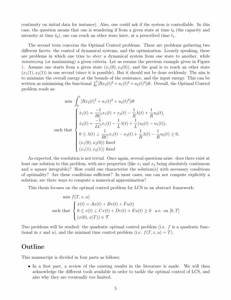
Linear Complementarity Systems are systems that are described by dynamical linear equations,which means that there is a variable, often named the state, which is changing with time. Theevolution of this variable is describe by a differential equation, which is linear. But also, this systemhas to comply with a constraint, which is expressed with complementarity. Complementarity meansthat two quantities can not be simultaneously active. In order to understand this properly, let usgive a simple physical example, found in [21].
L
i2
D λ
Ci1
R
u1
u2
Figure 1: Circuit with an ideal diode and twovoltage sources
Let us consider the circuit in Figure 1 witha diode D, resistance R and inductance L. Thediode in this case is considered to be ideal in thefollowing sense: it possesses a voltage/currentcharacteristic that translates the physical ob-servation.
• When the voltage λ is positive, then thecurrent i is cancelled.
• When the current i is negative, then thevoltage λ is cancelled.
This can be written mathematically as λ ≥ 0,i ≥ 0 and iλ = 0, which we rewrite morecompactly as 0 ≤ −i ⊥ λ ≥ 0. Denotex1(t) =
∫ t0i1(s)ds + x1(0) (the charge of the
capacitor, in coulomb) and x2(t) = i2(t) (theelectric current, in ampere). Then the evolu-tion of this system is described as:
x1(t) =−1
RCx1(t) + x2(t)− 1
Rλ(t) +
1
Ru2(t),
x2(t) =−1
LCx1(t)− 1
Lλ(t) +
1
L(u2(t)− u1(t)),
0 ≤ λ(t) ⊥ 1
RCx1(t)− x2(t) +
1
Rλ(t)− 1
Ru2(t) ≥ 0,
(1)
Several questions then arise. For instance, is the mathematical model valid? For this example,it means that the mathematical equation (1) has at least one solution once one sets the sourcefunction u, that the solution is preferably unique, and that it has some nice properties (like
4
continuity on initial data for instance). Also, one could ask if the system is controllable. In thiscase, the question means that one is wondering if from a given state at time t0 (the capacity andintensity at time t0), one can reach an other state later, at a prescribed time t1.
The second term concerns the Optimal Control problems. These are problems gathering twodifferent facets: the control of dynamical systems, and the optimization. Loosely speaking, theseare problems in which one tries to steer a dynamical system from one state to another, whileminimizing (or maximizing) a given criteria. Let us resume the previous example given in Figure1. Assume one starts from a given state (x1(0), x2(0)), and the goal is to reach an other state(x1(1), x2(1)) in one second (since it is possible). But it should not be done recklessly. The aim isto minimize the overall energy at the bounds of the resistance, and the input energy. This can bewritten as minimizing the functional
∫ 1
0[Rx2(t)2 +u1(t)2 +u2(t)2]dt. Overall, the Optimal Control
problem reads as:
min
∫ 1
0
[Rx2(t)2 + u1(t)2 + u2(t)2]dt
such that
x1(t) =−1
RCx1(t) + x2(t)− 1
Rλ(t) +
1
Ru2(t),
x2(t) =−1
LCx1(t)− 1
Lλ(t) +
1
L(u2(t)− u1(t)),
0 ≤ λ(t) ⊥ 1
RCx1(t)− x2(t) +
1
Rλ(t)− 1
Ru2(t) ≥ 0,
(x1(0), x2(0)) fixed(x1(1), x2(1)) fixed
As expected, the resolution is not trivial. Once again, several questions arise: does there exist atleast one solution to this problem, with nice properties (like x1 and x2 being absolutely continuousand u square integrable)? How could one characterize the solution(s) with necessary conditionsof optimality? Are these conditions sufficient? In most cases, one can not compute explicitly asolution; are there ways to compute a numerical approximation?
This thesis focuses on the optimal control problem for LCS in an abstract framework:
min f(T, x, u)
such that
x(t) = Ax(t) +Bv(t) + Fu(t)
0 ≤ v(t) ⊥ Cx(t) +Dv(t) + Eu(t) ≥ 0 a.e. on [0, T ]
(x(0), x(T )) ∈ T
Two problems will be studied: the quadratic optimal control problem (i.e. f is a quadratic func-tional in x and u), and the minimal time control problem (i.e. f(T, x, u) = T ).
OutlineThis manuscript is divided in four parts as follows:
• In a first part, a review of the existing results in the literature is made. We will thenacknowledge the different tools available in order to tackle the optimal control of LCS, andalso why they are eventually too limited.
5
• In a second part, a first attempt for tackling the quadratic optimal control problem for LCSis made. It relies on assumptions on the underlying complementarity conditions which turnsthe system into a Lipschitz system, non differentiable. Some first order conditions are thenderived, a first code to approximate the solution is written.
• In a third part, the results of Part 2 on the quadratic optimal control problem of LCS areenhanced. This time, properly defined multipliers are added to the necessary conditions,which are in turn transformed in order to be more efficiently handled. Also, these necessaryconditions are proved to be also sufficient. With these results, a code is developed in orderto compute an approximation of the solution. Two different approaches are tested, whichappear to be eventually complementary.
• Finally, the last part focuses on the minimal time problem for LCS. After extending someresults of the existing literature, these results are applied specifically on LCS in order toderive sufficient first order conditions. Then, a geometrical analysis of the shape of thecomplementarity constraints allows us to prove a bang-bang property for LCS.
6
List of publications
1. A. Vieira, B. Brogliato, and C. Prieur. Preliminary results on the optimal control of lin-ear complementarity systems. IFAC World Congress - Toulouse and IFAC-PapersOnLine,50(1):2977 – 2982, 2017.
2. A. Vieira, B. Brogliato, and C. Prieur. Quadratic Optimal Control of Linear Complement-arity Systems: First order necessary conditions and numerical analysis. Submitted to IEEETransactions on Automatic Control, January 2018.
A last paper, concerning the minimal time problem (content of Chapter 8) is under prepara-tion. These results were partly presented during the conference Control of state constraineddynamical systems (https://events.math.unipd.it/CoSCDS/) at the Department of Math-ematics Tullio-Levi Civita of Padua University, and during ISMP 2018 (https://ismp2018.sciencesconf.org/) in Bordeaux.
7

Part I
State of the art
8
Chapter 1
Linear Complementarity Systems
Abstract. In this chapter, the Linear Complementarity Systems (LCS) are presented. After someresults concerning the Linear Complementarity Problem (LCP), which is the specificity of thesesystems, some properties of the LCS are shown, with an effort for linking them with other types ofsystems appearing in the literature (like hybrid automata or differential inclusions). A last sectionfocuses on the numerical simulation of LCS.
At the core of the problem tackled by this thesis, one finds Linear Complementarity Systems(LCS). These dynamical systems are usually described as a linear dynamical system where one ofthe components is defined though a complementarity problem. More precisely, we call LCS(A(·),B(·), C(·), D(·)) the dynamical system:
x(t) = A(t)x(t) +B(t)λ(t)
0 ≤ λ(t) ⊥ C(t)x(t) +D(t)λ(t) ≥ 0
x(0) = x0 ∈ Rna.e. on [t0, t1] (1.1)
where t0, t1 ∈ R, t0 < t1, x : [t0, t1]→ Rn, λ : [t0, t1]→ Rm, and A(·), B(·), C(·), D(·) are matrices ofaccording dimensions. This provides a modeling paradigm for many problems, as Nash equilibriumgames, hybrid engineering systems [19], contact mechanics or electrical circuits [2].One could use the framework of differential inclusion in order to analyze solutions of problem(1.1), since λ(t) could be single or set valued depending on properties of the matrix D. Admitfor now that λ(t) is uniquely defined for every t ∈ [t0, t1] (for instance if D(t) is a P-matrix).As it will be stated in Section 1.1, λ is then a piecewise linear function of x. Therefore, theright-hand side defining the dynamics in (1.1) is a piecewise linear function of x, and thereforea Lipschitz function of x. Then, assuming that every matrix is a continuous function of time t,Cauchy-Lipschitz theorem proves that there exists a unique maximal solution x of (1.1) startingfrom x(t0) = x0 ∈ Rn (we could even argue that the solution exists on [t0, t1]).Since λ is a piecewise linear function of x, it means that the exists ` matrices Λi(·)`i=1 such that:
∃i ∈ `; x(t) = Λi(t)x(t), a.e. on [t0, t1]
It shows that there exists a connection between LCS and an other class of systems called switchingsystems. The latter ones encompass both continuous and discrete dynamics, and it has been apopular subject of study in recent years (see for instance [8]). This framework also generalizesDifferential Algebraic Equations (DAE), that are often non sufficient in order to describe mod-els naturally occurring in engineering problems that contain inequalities (for instance, unilateralconstraints) and disjunctive conditions (for conditional phenomena such as contacts).
9
1.1 Linear Complementarity ProblemsRoughly speaking, the Linear Complementarity Problem (LCP) is to find z ∈ Rn such that:
0 ≤ z ⊥Mz + q ≥ 0, (1.2)
where M ∈ Rn×n and q ∈ Rn is a given vector. This notation means that each component of z andMz+ q must be nonnegative, and both vectors must be perpendicular to each other, which in thiscase translates to:
zi(Mz + q)i = 0, ∀i ∈ 1, ..., n.One usually denotes the problem by LCP(q,M), and the set of its solution by SOL(q,M). Thisproblem appears naturally when one searches for first order conditions to a finite-dimensionaloptimization problem - also known as KKT conditions. Indeed, KKT conditions to a linear-quadratic problem of the form:
minz∈Rn
1
2zᵀHz + cᵀz
s.t.
Az ≥ b,
z ≥ 0,
where H ∈ Rn×n is a symmetric matrix, A ∈ Rm×n, b ∈ Rm, c ∈ Rn, are expressed as follows:
Hz + c− Aᵀλ− y = 0,
0 ≤ λ ⊥ Az − b ≥ 0,
0 ≤ y ⊥ z ≥ 0,
where y ∈ Rn, λ ∈ Rm are multipliers. By extracting y from the first equality, one obtains:
0 ≤(zλ
)⊥(H −AᵀA 0
)(zλ
)+
(c−b
)≥ 0.
The existence of solutions and their properties rely heavily on the structure of the matrix M .This chapter will present some results concerning the analysis of this problem that will be usefulfor the rest of this manuscript. Main information stated here can be found in [45].
1.1.1 Equivalent formulations
In order to analyze properties of the solutions of problem (1.2), we must reformulate the problemin an other framework.
Optimization problem As suggested by the former example, a first way is to express (1.2) asan optimization problem. It is easy to state the following proposition:
Proposition 1.1.1. Let q ∈ Rn, M ∈ Rn×n. z ∈ Rn is a solution of LCP (q,M) if and only if itis a global solution to the following quadratic problem:
minz∈Rn
zᵀ(Mz + q)
such that Mz + q ≥ 0,
z ≥ 0,
(1.3)
with an objective value of zero.
10

C-function A second way is to express this problem as finding the root of a two-argumentfunction, called C-function.
Definition 1.1.1. We call C-function a function f : R2n → Rn such that:
f(a, b) = 0 ⇐⇒ 〈a, b〉 = 0, a, b ≥ 0
If f is a C-function, then LCP(q,M) is equivalent to find z ∈ Rn such that f(z,Mz + q) = 0.Most known C-functions are:
• min function: z is a solution of LCP(q,M) iff min(z,Mz + q) = 0.
• Fischer-Burmeister’s C-function: z is a solution of LCP(q,M) iff√z2i + (Mz + q)2
i − (zi +(Mz + q)i) = 0, ∀i ∈ 1, n.
• normal map: z is a solution of LCP(q,M) iff Mz+ + q − z− = 0, where z+ = max(z, 0), andz− = max(−z, 0).
In general, C-functions are not Fréchet-differentiable, in particular at the origin. Even if thisreformulation seems appealing, this non-differentiability makes the use of this technique tricky inpractice. In relation with this fact, we introduce the notion of degeneracy of the solution.
Definition 1.1.2. A solution z of LCP(q,M) is said non-degenerate if for each i ∈ 1, ..., n,zi 6= (Mz + q)i.
If a solution is non-degenerate, then points in a neighbourhood around the solution are alsonon-degenerate. In this case, C-functions are usually Fréchet-differentiable, and locally convergentmethod for solving root problems of smooth functions (like the Newton method) will work efficientlyto solve this problem.
Piecewise affine functions The min function is of a special kind: it is a piecewise affinefunction. Such functions actually play a major role in the analysis of solutions of LCP. Moreformally speaking:
Definition 1.1.3. A function f : D → Rm, where D ⊆ Rn, is said to be piecewise affine functionif f is continuous and D is equal to the union of a finite number of convex polyhedra, called thepieces of f , on each of which f is an affine function.
The reformulation as the zero of a min-function already underlines the interaction between thetwo notions, but it goes even a bit further. Indeed, if f : Rn → Rn is an arbitrary piecewise affinefunction, then under a "nonsingularity" assumption, the system f(z) = 0 is equivalent to a certainLCP.Another link between these two notions lies in the next proposition:
Proposition 1.1.2. [45] Let M ∈ Rn×n be such that the LCP(q,M) has a unique solution for allvectors q ∈ Rn. Then the unique solution of the LCP(q,M) is a piecewise linear function of q.
11
Convex subdifferential Eventually, a final way to express the set of solutions is through thesubdifferential of the indicator function IR+
m, which is defined as:
IRm+ (x) =
0 if x ∈ Rm++∞ if x 6∈ Rm+ .
Since Rm+ is convex, its indicator function is also convex, and we can use tools of convex analysis, andin particular the subdifferential of a convex function. It can be proved easily that the subdifferentialof the indicator function ∂IRm+ (x) is equal to the normal cone of convex analysis NRm+ (x). It justifiesthe following equivalence:
0 ≤ z ⊥ ζ ≥ 0 ⇐⇒ −z ∈ NRm+ (ζ).
⇐⇒ −ζ ∈ NRm+ (z)
1.1.2 Class of matrices
A sensible question that may be asked is the following: what is the class of matrices M for whichLCP(q,M) has a solution for all vectors q ∈ Rn ? This class is denoted Q, and its elements arecalled Q-matrices. Unfortunately, there is no algebraic description allowing to check in finite timeif a matrix is a Q-matrix or not.
Global uniqueness If we narrow the problem by imposing uniqueness of the solution, we havemore comprehensive results.
Definition 1.1.4. A matrix M is said to be a P-matrix if LCP(q,M) admits a unique solutionfor all q ∈ Rn. The class of such matrices is denoted P.
The next theorem gives a full description of these P-matrices.
Theorem 1.1.1. [45] Let M ∈ Rn×n. The following statements are equivalent:
1. All principal minors of M are positive.
2. M reverses the sign of no nonzero vector, i.e.:
[zi(Mz)i ≤ 0 for all i] =⇒ [z = 0].
3. All real eigenvalues of M and its principal submatrices are positive.
4. M is a P-matrix.
A special subclass ofP-matrices are the symmetric positive definite matrices. From a symmetricpositive definite matrix M , one can define a norm: for x ∈ Rm, ‖x‖M =
√xᵀMx. With this, we
define the projection on a convex closed set K ⊂ Rn with the metric defined by M , denoted asprojK,M . In this sense, for all x ∈ Rn, projK,M(x) is the closest point to x in K according to ‖ · ‖M .Of course, if M is the identity matrix, then the usual projection operator is retrieved (simplydenoted as projK). In this framework, we have a formulation for the solution of an LCP.
Proposition 1.1.3. Let M ∈ Rn×n be a symmetric positive definite matrix and q ∈ Rn. Thereexists a unique x, solution of LCP(q,M), and:
x = projRn+,M(−M−1q
).
Proof. This is a simple application of Propositions 1.5.9 and 4.3.3 of [54].
12

Local uniqueness Asking for a global solution may be too restrictive. By pursuing the analogywith the necessary conditions of the optimization problems, rather than searching for a globalsolution, we could search for a local one. In other words, if z∗ is the solution of LCP(q,M), thenthere exist no other solution in a neighbourhood around z∗. This problem is entirely described asfollows:
Definition 1.1.5. A matrix M ∈ Rn×n is called nondegenerate if all its principal minors arenonzero.
Theorem 1.1.2. [45] Let M ∈ Rn×n. The following statements are equivalent:
1. M is nondegenerate.
2. For all vectors q, the LCP(q,M) has a finite number (possibly zero) of solutions.
3. For all vectors q, any solution of the LCP(q,M), if it exists, must be locally unique.
1.1.3 Numerical resolution
Of course, most LCP can not be solved analytically, but there exist several techniques to find anapproximate solution. There are two major families of techniques:
1. Pivoting techniques, based on the idea of pivoting as found in numerical algebra and linearprogramming. Examples as the criss-cross algorithm or Lemke’s algorithm show that theyterminate in a finite number of iterations (for a certain class of problems), but are in the worstcase of exponential complexity. Typically, these algorithms produce a sequence of vector pairs(yk, zk) that are extreme points of the feasible region (y, z)|y ≥ 0, z ≥ 0, y = Mz + qby moving inside the kernel of a basis matrix until a new boundary of the feasible region isencountered. These are good solutions for small to medium size problems, but the efficiencydecreases as the problem dimension increases, due to round-off errors and data storage.
2. Iterative methods, which do not solve the problem in finite number of iterations, but convergein the limit. They can exploit the sparsity of the problem, and are less sensitive to the round-off errors. A well known example are the interior point methods, which transform the problem(1.2) into the unconstrained minimisation problem:
min 〈x, y〉+ ‖y −Mx− q‖ − µ∑i
(log xi + log yi)
where µ > 0 is a parameter continuously driven to 0. As such, the solutions (x(µ), y(µ)) ofthis problem trace out a central path that leads to a solution of LCP(M, q). Interior methodsare well described in [111] and references therein.
1.2 Properties of the LCS
1.2.1 LCS seen as a hybrid automaton
Let us first describe LCS as hybrid automata to see the connection between them and stress thelimits. Notations exposed here are taken from [17].
13

Definition 1.2.1. A hybrid automaton is given by (Q,Σ, J, G) where:
• Q is a finite set of modes (sometimes called discrete states or locations).
• Σ = Σqq∈Q is a collection of dynamical systems. For mode q, these are given by the ODEx = fq(x) or by the DAE fq(x, x) = 0.
• J = Jqq∈Q. Jq ⊂ Rn is the jump set for mode q consisting of the states from which a modetransition and/or state jump occurs.
• G = Gq is the set of jump transition maps where Gq is a (possibly multi-valued) map fromJq to a subset of Rn ×Q.
Let’s now try to describe (1.1) as a hybrid automaton. The following description is inspiredby [63] and [64]. For simplicity of exposition, we denote y = Cx + Dλ and suppose A,B,C,Dautonomous.First, let us notice that the LCP states that λi(t) = 0 or yi(t) = 0 for each i ∈ n. This results in amultimodal system with 2m modes, where each mode is characterized by a subset I of m. Hence,Q = P(m), the power set of m. The dynamics fI in mode I are given by the DAE:
x = Ax+Bλ,
y = Cx+Dλ,
yi = 0, i ∈ Iλi = 0, i ∈ Ic
(1.4)
Also, the LCP imposes the sign condition:
λi(t) ≥ 0, i ∈ I, yi(t) ≥ 0, i ∈ Ic (1.5)
Therefore, the jump set JI is given by
JI = x0 ∈ Rn | there is no smooth solution (λ, x, y) of (1.4)for mode I satisfying x(0) = x0 and (1.5) on [0, ε[ for some ε > 0
A state x0 is said to be consistent for mode I if x0 6∈ JI . The set of consistent states for modeI is denoted VI . Define the set TI as the limit of the sequence:
T0 = 0, Ti+1 = x ∈ Rn|∃λ ∈ Rm, ∃x ∈ Ti such that x = Ax+Bλ, Cx+Dλ = y, yI = 0, λIc = 0
It is proved in [62] that this sequence converges in at most n steps. The jump transition functionG only depends on the state x(τ−) just before the event time τ , and not on the previous mode.The jump transition map is given by:
G(x) = (x+, I+) ∈ Rn × P(m)|x+ = ΠTI+VI+
(x) (1.6)
where ΠTIVI
is the projection onto VI along TI . There exist then different strategies to select a propertransition in G(x).
Presented that way, we see many computational drawbacks at converting back the LCS (1.1)in the framework of hybrid systems. First, the number of modes grow exponentially as m grows.Secondly, consistent spaces and transition maps are not easy to describe in a useful way. Even inthe case when the LCP condition defines λ uniquely, describing precisely the transition map is notan easy task: how do you choose the next mode I+?Even though this hybrid representation is an important tool for analysis, it is not the most efficientway to handle this system.
14
1.2.2 LCS seen as a differential inclusion
As it was shown in Section 1.1.1, the complementarity problem can be equivalently defined as theinclusion of the solution to a normal cone. Therefore, LCS(A,B,C, 0) can be equivalently definedas the Differential Inclusion (DI):
x ∈ Ax−BNRm+ (Cx) (1.7)
Suppose that there exists a symmetric positive definite matrix R such that R2B = Cᵀ and definez = Rx. Then one can prove (see [19, 20, 56]) that LCS(A,B, (R2B)ᵀ, 0) can be equivalentlyexpressed as the DI:
− z(t) +RAR−1z(t) ∈ NS(z(t)) (1.8)
where S = Rx|Cx ≥ 0. The equivalence is here understood in the sense that the two formalismsare strictly the same way of writing a mathematical object without consideration on the solution.A huge study of differential inclusions can be found in [98], where the author focuses on differentialinclusion of the type x ∈ F (x) for some multi-valued map F , but some hypothesis (such as aboundedness property of F ) put (1.7) out of its scope. The closest results concerning systems suchas (1.8) concern the sweeping process, introduced by Moreau [81]. Originally, a sweeping processis a differential inclusion defined as −x(t) ∈ NC(t)(x(t)), for some convex valued multifunctionC. These systems, under some hypothesis on C, admit some properties, such as uniqueness ofsolution for the Cauchy problem defined with this inclusion. Various forms of such systems havebeen analyzed; see for instance [3, 18, 30, 41, 68].
For a general system LCS(A,B,C,D), we have to put the system under the form of a DifferentialAlgebraic Inclusion (DAI). Create an auxiliary variable λ defined by Cx + Dv − λ = 0. Then,using the equivalence presented in Section 1.1.1, we know that −v ∈ NRm+ (λ). Reintroducing itinto the remaining equations, we obtain the DAI:
x− Ax ∈ −BNRm+ (λ)
Cx ∈ λ+DNRm+ (λ)(1.9)
Such systems are to date little studied. One can find some results in [26, 80].
1.2.3 Control of the LCS
Let us now turn to the control of such systems. There exist also some properties known for acertain class of LCS. Consider the input/output system:
x(t) = Ax(t) +Bλ(t) + Fu(t), (1.10a)
y(t) = Cx(t) +Dλ(t) + Eu(t), (1.10b)
0 ≤ λ(t) ⊥ y(t) ≥ 0, (1.10c)
where, compared to LCS(A,B,C,D), we just add an input u : [t0, t1] → Rk and F ∈ Rn×k,E ∈ Rm×k. There exist several results concerning properties satisfied by this system. We presenthere a few of them that will highlight some future results exposed later. In particular, these resultsshow that the set of absolutely continuous functions may be too small in order to define a statetrajectory x(·) solution of (1.10).
15

L2 solutions
The well-posedness of those systems have been analyzed in [32]. We summarise here their results.First of all, in order to state properly well-posedness for LCS, we must define clearly some concepts.
Definition 1.2.2. • LCS(A,B,C,D) is said to be passive (or dissipative with respect to thesupply rate 〈λ, y〉) if there exists a function V : Rn → R+ (called a storage function) suchthat:
V (x(t)) +
∫ t′
t
〈λ(t), y(t)〉dt ≥ V (x(t′))
holds for all t, t′ with t ≤ t′, and all (x, λ) ∈ L2([t, t′],Rn+m) satisfying (1.1) and y(t) =Cx(t) +Dλ(t).
• A function f : R+ → R is called Bohl function if it has a rational Laplace transform. Theset of such functions is denoted by B. We call f a Bohl distribution if f = freg + fimp withthe impulsive part fimp =
∑`i=0 uiδ
(i)0 , where δ0 the Dirac function centered at 0, and δ(i)
0 isits ith derivative, and the regular part freg ∈ B.
• A Bohl distribution f is initially nonnegative if its Laplace transform f satisfies f(σ) ≥ 0 forsufficiently large σ.
• f is said to be a piecewise Bohl function if f is right-continuous and there exists a collectionof isolated points Γw = τi ⊆ R+ (called the transition points) such that for every i, thereexists a function g ∈ B such that f (ti,ti+1) = g (ti,ti+1). We denote this space PB.
• The distribution space L2,δ(R+) is defined as the set of all u = uimp + ureg where uimp =∑θ∈Γ uθδθ for uθ ∈ R with a set of isolated points Γ ⊂ R+ and ureg ∈ L2
loc(R+).
Definition 1.2.3 (Initial solution). The Bohl distribution (v, x, y) is an initial solution to (1.10)with initial state x0 and input u ∈ B if:
1. The equations x = Ax+Bv+Eu+ x0δ, y = Cx+Dv+Fu hold in the distributional sense.
2. There exists a J ⊆ m such that vi = 0, i ∈ m\J and yi = 0, i ∈ J , as equalities ofdistributions.
3. The distributions v and y are initially nonnegative.
In the following Theorem, we denote by ΓEu the set of times when Eu(·) is discontinuous.
Theorem 1.2.1. [32, Theorem 7.5] Consider an LCS given by (1.10) such that LCS(A,B,C,D) is
passive with the storage function x 7→ 12xᵀKx for some matrix K positive definite, and
(B
D +Dᵀ
)has full column rank. Then, for any initial state x0 and any input function u ∈ PBm, (1.10) admitsa unique global solution (x, y, v) ∈
(L2,δ(R+)
)n+m+m satisfying:
1. ximp = 0, and impulses in (v, y) only show up at times in Γ = 0 ∪ ΓEu.
16
2. For any interval (a, b) such that (a, b) ∩ Γ = ∅, xreg (a,b)is absolutely continuous and satisfy
for almost all t ∈ (a, b):
xreg(t) = Axreg(t) +Bvreg(t) + Fu(t)
yreg(t) = Cxreg(t) +Dvreg(t) + Eu(t)
0 ≤ vreg(t) ⊥ yreg(t) ≥ 0
3. For each θ ∈ Γ, the corresponding impulse (yθδθ, vθδθ) is equal to the impulsive part of theunique initial solution to (1.10) with initial state xreg(θ
−) and input t 7→ u(t− θ).
4. For time θ ∈ Γ, it holds that xreg(θ+) = xreg(θ−) +Buθ.
Some results where the solutions of LCS encompass higher order derivatives of the Dirac func-tion may be found in [3, 63].
BV solutions
Suppose D = 0 and there exists a matrix R symmetric positive definite such that R2B = Cᵀ.Resuming the presentation made in Section 1.7, one can prove (see [22]) that (1.10) is equivalentlydefined as the perturbed sweeping process :
− z(t) +RAR−1z(t) +RFu(t) ∈ NS(t)(z(t)) (1.11)
where S(t) = Rx|Cx + Eu(t) ≥ 0. The term perturbed comes from the fact that the termRAR−1z(t) + RFu(t) is added. The perturbed sweeping processes offer a framework allowing fora different analysis.Let us state first some definitions. The variation of x(·) on [t0, t1] is the supremum of
∑‖x(ti)−
x(ti−1)‖ over the set of all finite sets of points t2 < ... < tk of [t0, t1]. When this supremum is finite,the mapping x(·) is said to be of bounded variation on [t0, t1]. x(·) is of locally bounded variationon [t0, t1] if it is of bounded variation on each compact subinterval of [t0, t1].Considering a set-valued mapping S : [t0, t1] ⇒ Rn and replacing the above expression ‖z(ti) −z(ti−1)‖ by the Hausdorff distance haus(S(ti), S(ti−1)), one obtains the concept of set valued map-pings with (locally) bounded variation on [t0, t1]. The Hausdorff distance between two subsets Q1
and Q2 in Rn is given by
haus(Q1, Q2) = max
supx∈Q1
infy∈Q2
‖x− y‖, supx′∈Q2
infy′∈Q1
‖x′ − y′‖
Denoting by varS(t) the variation of S(·) over [t0, t], S(·) is said locally absolutely continuous on[t0,+∞[ if varS(·) is locally absolutely continuous on [t0,+∞[.We make the following assumption on (1.10):
Assumption 1.2.1. Let D = 0. There exists a symmetric positive definite matrix R such thatR2B = Cᵀ.
Given u : [t0,+∞[→ Rm, define K(t) = x ∈ Rn|Cx + Fu(t) ≥ 0. We can now state thewell-posedness theorem:
17

Theorem 1.2.2. [22, Theorem 3.5] Assume that u(·) ∈ L1loc([t0,+∞[,Rm), that Assumption 1.2.1
holds and that the set-valued mapping S(·) = R(K(·)) is locally absolutely continuous (resp. rightcontinuous of locally bounded variation) with nonempty values. Then (1.10) with initial conditionx(0) ∈ R(K(0)) has one and only one locally absolutely continuous (resp. right continuous oflocally bounded variation) solution x(·) on [0,+∞[.
This result can be extended to the case D ≥ 0 or even for nonlinear systems, under somefurther hypothesis.The fact that a solution of the differential equation (1.10) may be only right continuous and oflocally bounded variation may seem unnatural. This is due to a reformulation of (1.10) into ameasure differential inclusion [81], which extends the notion of differential inclusions in order toinclude state jumps representations. This result will explain some results obtained in numericalsimulation presented in Chapter 7.Also, this may seem in contradiction with the results presented in the previous paragraph aboutL2 solutions. Actually, these two results are different: the former solution concept proves globalexistence and uniqueness of a solution x(·) on L2(R+), and the latter proves the global existenceand uniqueness of a solution right continuous with bounded variation. Since a function may belongto L2(R+) and not be right continuous of bounded variation (and vice versa), these two results areactually different.
Complete controllability of a class of LCS
First, let us formulate an Assumption on (1.10):
Assumption 1.2.2. The following conditions are satisfied for the LCS (1.10)
• The matrix D is a P-matrix.
• The transfer matrix E + C(sI − A)−1F is invertible as a rational matrix.
These assumptions are actually really restrictive, but they make the analysis easier. The secondassumption for instance requires that the number of inputs and the number of complementarityvariables be the same. It follows from the first assumption that for each initial state x0 and boundedlocally integrable input u there exist a unique absolutely continuous state trajectory xx0,u andlocally integrable trajectories (λx0,u, yx0,u) such that xx0,u(0) = x0 and the triple (xx0,u, λx0,u, yx0,u)satisfies the relations (1.10) for almost all t ≥ 0.A major result concerning (1.10) is on the complete controllability of the system. We recall thedefinition here:
Definition 1.2.4. The LCS (1.10) is said completely controllable if for any pair of states (x0, xf ) ∈Rn+n, there exists a locally integrable input u such that the associated trajectory xx0,u satisfiesxx0,u(t1) = xf .
Theorem 1.2.3. [31] Consider an LCS (1.10) satisfying Assumption 1.2.2. It is completely con-trollable if and only if the following two conditions hold:
1. The pair (A, [F,B]) is controllable.
2. The system of inequalitiesη ≥ 0 (1.12a)
18
(ξᵀ ηᵀ
)(A− νI FC E
)= 0 (1.12b)
(ξᵀ ηᵀ
)(BD
)≤ 0 (1.12c)
admits no solution ν ∈ R and 0 6= (ξ, η) ∈ Rn+m.
1.2.4 Zeno behavior
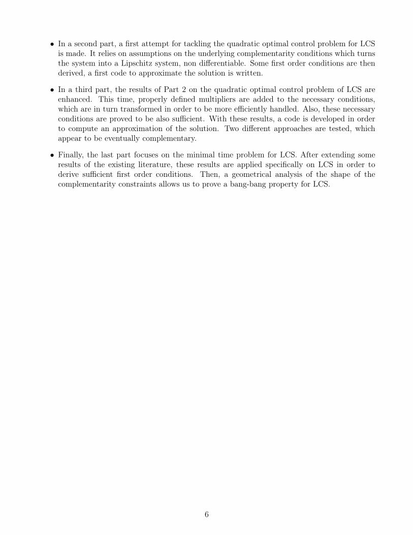
This definition of solution hides a detail. In the community dealing with switching systems, anassumption is often made: the trajectory admits no Zeno-state, meaning there is no time with aninfinite accumulation of switch events. We define here more precisely what is the Zeno phenomenon.From LCS(A,B,C,D) (1.1), define three sets of indices, two called the active sets:
I+0t (x, λ) = i ∈ m : λi(t) > 0 = Cx(t) +Dλ(t) (1.13a)
I0+t (x, λ) = i ∈ m : λi(t) = 0 < Cx(t) +Dλ(t) (1.13b)
and the last called the degenerate set:
I00t (x, λ) = i ∈ m : λi(t) = 0 = Cx(t) +Dλ(t) (1.13c)
Definition 1.2.5. Let (x, λ) be a solution trajectory of (1.1), t∗ ∈ [t0, t1], and let x(t∗) = x∗. Wesay x∗ is:
• left non-Zeno relative to (x, λ) if a scalar ε− > 0 and a triple of index sets (I0+− , I+0
− , I00− )
exists such that (I0+− , I+0
− , I00− ) = (I0+
t (x, λ), I+0t (x, λ), I00
t (x, λ)) for every t ∈ [t∗ − ε−, t∗[.
• right non-Zeno relative to (x, λ) if a scalar ε+ > 0 and a triple of index sets (I0++ , I+0
+ , I00+ )
exists such that (I0++ , I+0
+ , I00+ ) = (I0+
t (x, λ), I+0t (x, λ), I00
t (x, λ)) for every t ∈]t∗, t∗ + ε+].
When x∗ is left and right non-Zeno, then we say that x∗ is non-Zeno.
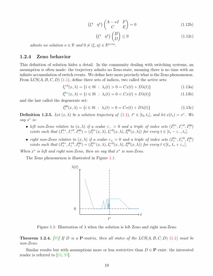
The Zeno phenomenon is illustrated in Figure 1.1.
t
λ(t)
0
t∗
Figure 1.1: Illustration of λ when the solution is left Zeno and right non-Zeno
Theorem 1.2.4. [97] If D is a P-matrix, then all states of the LCS(A,B,C,D) (1.1) must benon-Zeno.
Similar results but with assumptions more or less restrictive than D ∈ P exist: the interestedreader is referred to [33, 97].
19
1.2.5 Dependence to initial conditions
Consider the Boundary Value Problem (BVP):
x = Ax+Bλ
0 ≤ λ ⊥ Cx+Dλ ≥ 0
Mx(0) +Nx(T ) = b
(1.14)
where the system is described the same way as in (1.1) but a boundary condition is added (insteadof an initial value), defined with matrices M,N ∈ R2n×n and b ∈ R2n. In the smooth cases, solvingBVP uses a technique called shooting, which needs a sensitivity in the variation of the trajectorygiven changes in the initial condition. This sensitivity is usually given by a Jacobian matrix, whichis defined though a differential equation involving the derivative of the right-hand side functionin the dynamical system. In the case of (1.14), since λ is not a differentiable function of x, thisproperty does not hold. However, Pang and Stewart [85] derived a result giving a sensitivity matrix(through a weaken sense of derivation), which leads to a non-smooth Newton method.
Definition 1.2.6. • A set-valued map F : X ⇒ Y , where X and Y are normed space, issaid upper semi-continuous at x0 ∈ X if for all open set M containing F (x0), there is aneighbourhood Ω of x0 such that F (Ω) ⊂ M . F is said upper semi-continuous if it is so atevery point x0 ∈ X.
• Let Φ : D ⊆ Rn → Rn be a vector function defined on the open set D. The function Φ issaid to have a linear Newton approximation at x ∈ D if for an open neighborhood of x, aset-valued map T : N ⇒ Rn×n exists such that:
(a) T (x) is a non empty compact subset of n× n matrices for every x ∈ N ,
(b) T is a upper semicontinuous at x,
(c) there exists a scalar function ∆ : R+ → R+ satisfying lims↓0
∆(s) = 0 such that for all
x ∈ N and all E ∈ T (x),
‖Φ(x)− Φ(x)− E(x− x)‖ ≤ ‖x− x‖∆(‖x− x‖).
If (c) is strengthened to
(c’) a constant c > 0 exists such that for all x ∈ N and all E ∈ T (x),
‖Φ(x)− Φ(x)− E(x− x)‖ ≤ c‖x− x‖2,
then we say that the linear Newton approximation T is strong.
Linear Newton approximations generalize the concept of Jacobian matrix for a broad class offunctions (broader than C 1 functions), and allow us to design a nonsmooth Newton method inorder to solve the equation Φ(x) = 0 with Φ non differentiable.Let us use this definition for the solution map of (1.14). Define L(z) as the family of index setsconsisting of all α satisfying:
1. there exists a solution λ to the LCP(Cz,D) such that i : λi > 0 ⊆ α ⊆ J = i :(Cz +Dλ)i = 0,
20
2. the columns of the matrix DJα are linearly independent.
By convention, we let L(z) consists of only the empty set if no such index set α exists.
Theorem 1.2.5. [85] Suppose B SOL(Cx,D) is a singleton for all x ∈ Rn. For ξ ∈ Rn, denoteby x(·, ξ) a solution of the IVP (1.1) with initial condition x(0, ξ) = ξ.
• Define the family
Th(x) = −B•α[(DJα)ᵀDJα]−1(DJα)ᵀCJ• : α ∈ L(x).
If L(x) = ∅, then Th(x) consists of only the zero matrix. Then Th provides a linear Newtonapproximation for the piecewise linear function x 7→ B SOL(Cx,D).
• Define Φb(ξ) = Mξ+Nx(t1, ξ)−b. Let us consider the Differential Inclusion (DI) in matrix:
Y (t) ∈ AY (t) + (convTh(x(t, ξ)))Y (t), Y (0) = I, (1.15)
where I is the identity matrix. Then TΦ(ξ) = M + NY (t1) : Y (·) solves the DI (1.15) isa linear Newton approximation of Φb.
• Suppose the BVP (1.14) has a solution x(·; ξ∗). If all matrices M+NY ∗(t1) are nonsingular,where Y ∗ is a solution of the Differential Inclusion (1.15) with ξ = ξ∗, then there exists aneighbourhood N∗ of ξ∗ such that for any initial iterate ξ0 chosen from N∗, the sequence ξkwhere
ξk+1 = (M + NY k(t1))−1(xb + N(Y k(t1)ξk − x(t1, ξk))), ∀k ≥ 0
where Y k is a solution of the DI (1.15) with ξ = ξk, is well defined, remains in N∗ andconverges Q-superlinearly to ξ∗, meaning:
limk→∞
‖ξk+1 − ξ∗‖‖ξk − ξ∗‖
= 0.
However, the assumption that x 7→ B SOL(Cx,D) is single-valued for all z is binding. Indeed,as it was noted in [84, Proposition 5.1], the single-valuedness of x 7→ B SOL(Cx,D) on Rn is anecessary and sufficient condition for the initial-value LCS (1.1) to have a unique C 1 trajectoryx(·, x0) for all initial conditions x0 ∈ Rn.
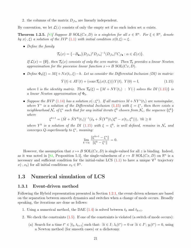
1.3 Numerical simulation of LCS
1.3.1 Event-driven method
Following the Hybrid representation presented in Section 1.2.1, the event-driven schemes are basedon the separation between smooth dynamics and switches when a change of mode occurs. Broadlyspeaking, the iterations are done as follows:
1. Using a numerical method, the DAE (1.4) is solved between tk and tk+1.
2. We check the constraints (1.5). If one of the constraints is violated (a switch of mode occurs):
(a) Search for a time t∗ ∈ [tk, tk+1] such that: ∃i ∈ I; λi(t∗) = 0 or ∃i ∈ Ic; yi(t∗) = 0, usinga Newton method (for smooth cases) or a dichotomy.
21
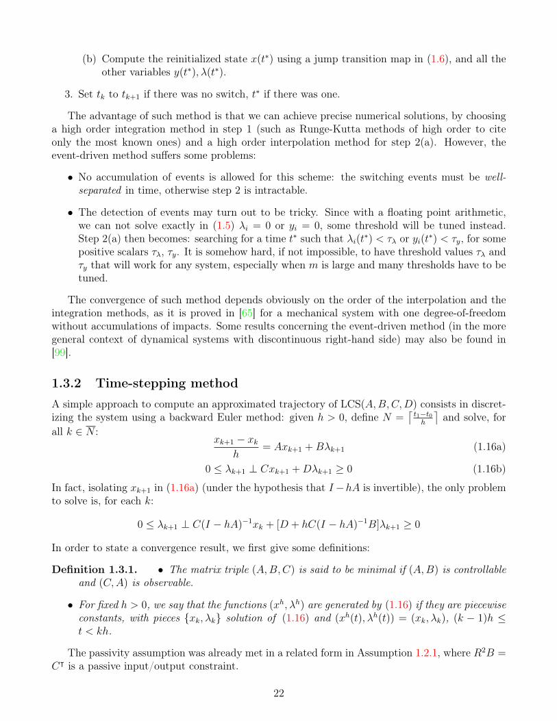
(b) Compute the reinitialized state x(t∗) using a jump transition map in (1.6), and all theother variables y(t∗), λ(t∗).
3. Set tk to tk+1 if there was no switch, t∗ if there was one.
The advantage of such method is that we can achieve precise numerical solutions, by choosinga high order integration method in step 1 (such as Runge-Kutta methods of high order to citeonly the most known ones) and a high order interpolation method for step 2(a). However, theevent-driven method suffers some problems:
• No accumulation of events is allowed for this scheme: the switching events must be well-separated in time, otherwise step 2 is intractable.
• The detection of events may turn out to be tricky. Since with a floating point arithmetic,we can not solve exactly in (1.5) λi = 0 or yi = 0, some threshold will be tuned instead.Step 2(a) then becomes: searching for a time t∗ such that λi(t∗) < τλ or yi(t∗) < τy, for somepositive scalars τλ, τy. It is somehow hard, if not impossible, to have threshold values τλ andτy that will work for any system, especially when m is large and many thresholds have to betuned.
The convergence of such method depends obviously on the order of the interpolation and theintegration methods, as it is proved in [65] for a mechanical system with one degree-of-freedomwithout accumulations of impacts. Some results concerning the event-driven method (in the moregeneral context of dynamical systems with discontinuous right-hand side) may also be found in[99].
1.3.2 Time-stepping method
A simple approach to compute an approximated trajectory of LCS(A,B,C,D) consists in discret-izing the system using a backward Euler method: given h > 0, define N =
⌈t1−t0h
⌉and solve, for
all k ∈ N :xk+1 − xk
h= Axk+1 +Bλk+1 (1.16a)
0 ≤ λk+1 ⊥ Cxk+1 +Dλk+1 ≥ 0 (1.16b)
In fact, isolating xk+1 in (1.16a) (under the hypothesis that I−hA is invertible), the only problemto solve is, for each k:
0 ≤ λk+1 ⊥ C(I − hA)−1xk + [D + hC(I − hA)−1B]λk+1 ≥ 0
In order to state a convergence result, we first give some definitions:
Definition 1.3.1. • The matrix triple (A,B,C) is said to be minimal if (A,B) is controllableand (C,A) is observable.
• For fixed h > 0, we say that the functions (xh, λh) are generated by (1.16) if they are piecewiseconstants, with pieces xk, λk solution of (1.16) and (xh(t), λh(t)) = (xk, λk), (k − 1)h ≤t < kh.
The passivity assumption was already met in a related form in Assumption 1.2.1, where R2B =Cᵀ is a passive input/output constraint.
22
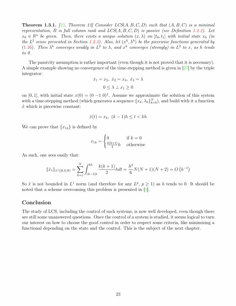
Theorem 1.3.1. [27, Theorem 13] Consider LCS(A,B,C,D) such that (A,B,C) is a minimalrepresentation, B is full column rank and LCS(A,B,C,D) is passive (see Definition 1.2.2). Letx0 ∈ Rn be given. Then, there exists a unique solution (x, λ) on [t0, t1] with initial state x0 (inthe L2 sense presented in Section 1.2.3). Also, let (xh, λh) be the piecewise functions generated by(1.16). Then λh converges weakly in L2 to λ, and xh converges (strongly) in L2 to x, as h tendsto 0.
The passivity assumption is rather important (even though it is not proved that it is necessary).A simple example showing no convergence of the time-stepping method is given in [27] by the tripleintegrator:
x1 = x2, x2 = x3, x3 = λ
0 ≤ λ ⊥ x1 ≥ 0
on [0, 1], with initial state x(0) = (0 −1 0)ᵀ. Assume we approximate the solution of this systemwith a time-stepping method (which generates a sequence xk, λkNk=0), and build with it a functionx which is piecewise constant:
x(t) = xk, (k − 1)h ≤ t < kh
We can prove that x1k is defined by
x1k =
0 if k = 0k(k+1)
2h otherwise
As such, one sees easily that:
‖x1‖L1([0,1],R) =N∑k=1
∫ kh
(k−1)h
k(k + 1)
2hdt =
h2
6N(N + 1)(N + 2) = O
(h−1)
So x is not bounded in L1 norm (and therefore for any Lp, p ≥ 1) as h tends to 0. It should benoted that a scheme overcoming this problem is presented in [3].
Conclusion
The study of LCS, including the control of such systems, is now well developed, even though thereare still some unanswered questions. Once the control of a system is studied, it seems logical to turnour interest on how to choose the good control in order to respect some criteria, like minimizing afunctional depending on the state and the control. This is the subject of the next chapter.
23

Chapter 2
Non-smooth Optimal Control Problems
Abstract. This chapter focuses on the optimal control of various types of dynamical systemson two different aspects. First of all, the necessary conditions of optimality concerning differentsystems are considered, including hybrid automata, differential inclusions, Lipschitz systems andmixed constraints. Along these lines, the presentation will show the limitations of these resultswhen they are applied to LCS. Secondly, two methods of numerical approximations of the optimalsolutions are presented, called respectively the Direct and Indirect methods.
Let us now focus on the analysis of Optimal Control Problems. These problems, which findtheir origin in the Calculus of Variation, have many applications in a wide variety of topics.Mathematically speaking, these problems are formulated as the optimization of a functional overfunctions satisfying a differential equation (or a differential inclusion), alongside with constraintsover the whole domain of integration and/or at the boundaries. We focus here only on OptimalControl Problems of Ordinary Differential Equations of the form:
min
∫ T
0
gint(t, x(t), u(t))dt+ gb(x(0), x(T ))
s.t.
x(t) = f(t, x(t), u(t))
gc(t, x(t), u(t)) ∈ E(t)
(x(0), x(T )) ∈ Ba.e. on [0, T ],
(2.1)
where x : [0, T ] → Rn is called the state, u : [0, T ] → Rm is called the control, gint : [0, T ] × Rn ×Rm → R called the running cost, gb : R2n → R called the final cost, f : [0, T ] × Rn × Rm → Rn,gc : [0, T ]× Rn × Rm → Rk, E : [0, T ]⇒ Rk, B ⊆ R2n. Further hypothesis can be made concerningsmoothness of functions appearing in (2.1), making the analysis of this problem more or less easy.Several names are given to this problem whether the running cost gint and the final cost gb arepresent or not. We call it a Mayer problem if gint ≡ 0, a Lagrange problem if gb ≡ 0, and a Mayerproblem if none of them is identically 0.By analogy with what is made for finite-dimensional optimization problems, the analysis of (2.1)often focuses on two different topics: existence of an optimal solution, and searching for necessaryconditions that the optimal solution should comply with. For Optimal Control Problems, theseconditions take the form of the Pontryagin equations, defining an adjoint state through a Differ-ential Algebraic Equation. These first order necessary conditions were first proved by Pontryaginet al in their seminal work (see [88]). Their work focused on optimal control with smooth data,and only constraints in the control were allowed. We state here their version for illustration:
24
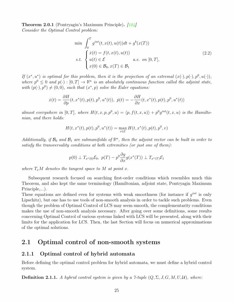
Theorem 2.0.1 (Pontryagin’s Maximum Principle). [104]Consider the Optimal Control problem:
min
∫ T
0
gint(t, x(t), u(t))dt+ gb(x(T ))
s.t.
x(t) = f(t, x(t), u(t))
u(t) ∈ Ex(0) ∈ B0, x(T ) ∈ B1
a.e. on [0, T ],
(2.2)
If (x∗, u∗) is optimal for this problem, then it is the projection of an extremal (x(·), p(·), p0, u(·)),where p0 ≤ 0 and p(·) : [0, T ] → Rn is an absolutely continuous function called the adjoint state,with (p(·), p0) 6= (0, 0), such that (x∗, p) solve the Euler equations:
x(t) =∂H
∂p(t, x∗(t), p(t), p0, u∗(t)), p(t) = −∂H
∂x(t, x∗(t), p(t), p0, u∗(t))
almost everywhere in [0, T ], where H(t, x, p, p0, u) = 〈p, f(t, x, u)〉 + p0gint(t, x, u) is the Hamilto-nian, and there holds:
H(t, x∗(t), p(t), p0, u∗(t)) = maxv∈E
H(t, x∗(t), p(t), p0, v)
Additionally, if B0 and B1 are submanifolds of Rn, then the adjoint vector can be built in order tosatisfy the transversality conditions at both extremities (or just one of them):
p(0) ⊥ Tx∗(0)E0, p(T )− p0 ∂g
∂xg(x∗(T )) ⊥ Tx∗(T )E1
where TxM denotes the tangent space to M at point x.
Subsequent research focused on searching first-order conditions which resembles much thisTheorem, and also kept the same terminology (Hamiltonian, adjoint state, Pontryagin MaximumPrinciple,...).These equations are defined even for systems with weak smoothness (for instance if gint is onlyLipschitz), but one has to use tools of non-smooth analysis in order to tackle such problems. Eventhough the problem of Optimal Control of LCS may seem smooth, the complementarity conditionsmakes the use of non-smooth analysis necessary. After going over some definitions, some resultsconcerning Optimal Control of various systems linked with LCS will be presented, along with theirlimits for the application for LCS. Then, the last Section will focus on numerical approximationsof the optimal solutions.
2.1 Optimal control of non-smooth systems
2.1.1 Optimal control of hybrid automata
Before defining the optimal control problem for hybrid automata, we must define a hybrid controlsystem.
Definition 2.1.1. A hybrid control system is given by a 7-tuple (Q,Σ, J, G,M,U,U), where:
25
• (Q,Σ, J, G) is a hybrid automaton as defined in Definition 1.2.1 (where this time, Σ is definedthrough ODEs of the form x = fq(t, x, u)).
• M = Mqq∈Q is a collection of smooth manifolds where the state can have values for eachmode.
• U = Uqq∈Q is a collection of sets defining acceptable values for the control for each mode.
• U = Uqq∈Q is a collection of functional sets admissible for controls: u :Dom(u)→ Uq.
Optimal control of such systems have been widely analyzed: see for instance [11, 29, 49, 55,86, 87, 101, 102, 105, 106]. The functional to minimize may take into account a running costpartitioned over the different modes followed by the trajectory, along with a cost on the state atswitching times; the switching times may also be part of the optimal solution searched. As it wasunderlined in Section 1.2.1, this approach has a lot of drawbacks for LCS:
• First of all, describing the LCS as a switching system is not an easy task, and the resultingsystem may become too big to apply properly these results (for instance, because of the 2m
different modes possible);
• Secondly, most results concerning the Optimal Control of Switching Systems only assumethat the dynamical systems are described with ODEs for each mode. However, in most casesof LCS, the dynamical system will be described with DAEs. Furthermore, adding furtherconstraints involving at the same time the state and the control does not seem to be takeninto account in the above articles;
• The resulting necessary conditions make strong assumptions on the system, on the admissibletransitions at switching times, or on the number of switches on the interval of integration.Therefore, the results become intractable for a high number of switches or modes.
For all these reasons, the hybrid approach will not be used in order to tackle the Optimal Controlproblem for LCS.
2.1.2 Differential inclusions and the sweeping process
The Optimal Control Problem for Differential Inclusions also attracted a lot of interest. Wesummarize here some results concerning this.
Lipschitz bounded differential inclusions
In [98], the problem of optimality of solution is tackled for system of the form x ∈ F (x) for somemultifunction F : Rn ⇒ Rn complying with some assumptions. Let F : Rn ⇒ Rn be a uppersemi-continuous multifunction (see Definition 1.2.6) with compact convex values. The problem isthen to solve:
min φ(x(T ))
s.t.
x ∈ F (x)
x(0) ∈ C0, x(T ) ∈ C1
(2.3)
over absolutely continuous functions x : [0, T ] → Rn, where C0, C1 are two closed subsets of Rn,and φ : Rn → R is a Lipschitz function. One could see this problem as a generalization of optimal
26
control of systems defined by the ODE x = f(x, u), u ∈ U (by defining F (x) = f(x, U)). For thisproblem, one can prove two results: one concerning existence of an optimal solution, one givingnecessary condition this optimal solution should comply with [98, 109]. These conditions are closeto the PMP.
However, since the multifunction F is supposed to have compact values, we can not apply itdirectly to the controlled LCS (1.11). Indeed, except for some peculiar cases, the normal cone,seen as a multifunction, may admit unbounded values; for instance, NR+(0) = −R+.
Sweeping process
The optimal control of sweeping processes −x ∈ NC(t)(x(t)) (see Section 1.2.3) has been a topicof research gathering a lot of attention in the recent past years. Of course, as it was mentioned inSection 1.2.3, a Cauchy problem described with a sweeping process may admit a unique solution;there is, in these cases, no hope to optimize any trajectory, unlike in many cases of systems definedwith a differential inclusion. In the literature, three different approaches attempt to add controlin the sweeping process:
1. Adding an additive perturbation in the differential inclusion, taking the form
−x ∈ NC(t)(x(t)) + f(t, x(t), a(t))
for some function a : [0, T ]→ Rm and f : [0, T ]× Rn+m → Rn, and where C(·) is unchanged.The research in this direction mainly focuses on existence and relaxation; see [5, 6, 44, 77]and references therein.
2. The second approach couples a sweeping process and a controlled ordinary differential equa-tion, where C(t) is a given multimap but uncontrolled. The results provide necessary optim-ality conditions [4, 23].
3. The third approach adds control in the definition of the moving set. For instance, [43] focuseson the case of moving controlled polyhedra:
C(t) = x ∈ Rn | 〈ui(t), x〉 ≤ bi(t), i = 1, ...,m
where the control functions are ui and bi, i = 1, ...,m. The results focus on necessaryoptimality conditions: see [42, 43]. As noted in [28], the discrete approximation approachto optimization of the differential inclusions x ∈ F (x) (see [79]) heavily relies on a Lipschitzproperty of the multifunction F . However, this assumption is not verified with such controlledpolyhedra, and therefore the approach can not be applied.
The closest result to the optimal control problem of LCS may be found in [28], where the optimalcontrol problem reads as:
min φ(x(T )) +
∫ T
0
`(t, x(t), u(t), a(t), x(t), u(t), a(t))dt
s.t.
− x(t) ∈ NC(t)(x(t)) + f(x(t), a(t))
C(t) = C + u(t), C = x ∈ Rn | Gx ≥ 0‖u(t)‖ = r
27
for φ : Rn → R, ` : [0, T ] × R4n+2d → R, a scalar r > 0 and a matrix G ∈ Rm×n, and where thecontrols are a : [0, T ]→ Rd and u : [0, T ]→ Rn. If one supposes f(x, a) = −Ax− Fa, the systemcan be easily put in the form of a LCS. Notice that C(t) = x ∈ Rn|Gx + Gu(t) ≥ 0. Moreover,using [22, Proposition A.2], we prove that:
∂IC(t)(x) = Gᵀ∂IRm+ (Gx+ Eu(t))
where IK is the indicator function of the setK and ∂ denotes the convex subdifferential (see Section1.2.2). Therefore, since ∂IK(x) = NK(x), it yields: −x ∈ GᵀNRm+ (Gx + Gu) + Ax + Fa. Finally,we use the following equivalence (presented Section 1.1.1):
−v ∈ NRn+(Gx+Gu) ⇐⇒ 0 ≤ v ⊥ Gx+Gu ≥ 0
such that we prove the equivalence between the sweeping process and the following LCS:
x(t) = Ax(t) +Gᵀv(t) + Fa(t)
0 ≤ v(t) ⊥ Gx(t) +Gu(t) ≥ 0
‖u(t)‖ = r
The main results of [28] show well-posedness of the system, convergence of the discrete approxima-tions, and necessary optimality conditions. However, the results developed in [28] do not apply toour problem because of the presence of decoupled controls (u, a), acting either on the polyhedronor on the dynamical inclusion.
2.1.3 Lipschitz systems
As presented in Proposition 1.1.2, a certain class of LCS can be described with a piecewise linearLipschitz differential equation, but not differentiable. Most results concerning optimality analysisof non constrained systems require some differentiability of the data, but this assumption has to beweakened. Clarke in [40] tackled the optimal control problem of a non-constrained system underminimal hypotheses; namely, the data have to be measurable and Lipschitz in the state variable.We state here more clearly his results, as they will be used in further development.
Definition 2.1.2. Let g : Rn → Rk be a locally Lipschitz function. We define the Clarke generalizedJacobian ∂Cg(s) of g at s as:
∂Cg(s) = conv(lim(Dg(si))ᵀ)
where we consider all sequences si converging to s where the usual Jacobian Dg(si) exists, aswell as the limit of the sequence Dg(si). For f : Rn × R` → Rk, we denote by ∂Cs f(t, x) theClarke generalized partial Jacobian, which is the generalized Jacobian of the function s 7→ f(t, s)at point x.
Consider the following optimal control problem:
min
∫ T
0
f 0(t, x(t), u(t))dt
s.t.
x(t) = f(t, x(t), u(t)
u(t) ∈ U(t), x(t) ∈ Xx(0) ∈ C0, x(T ) ∈ C1
(2.4)
28
where T > 0 is given, f 0 : [0, T ]× Rn × R, f : [0, T ]× Rn × Rm, U : [0, T ]⇒ Rm is a multifunction,X, C0 and C1 are closed subsets of Rn. u : [0, T ] → Rm satisfying u(t) ∈ U(t) a.e. t ∈ [0, T ] isa Lesbesgue measurable function (the control). An admissible trajectory associated with u is anabsolutely continuous function x : [0, T ]→ Rn satisfying the constraints in (2.4) and x(t) ∈ X a.e.on [0, T ]. x is said interior if moreover, x(t) ∈ int X a.e.
Define f = (f, f0). We do the following hypotheses:
H1 For each s in a neighborhood of X, the function (t, u) 7→ f(t, s, u) is L×Bm-measurable1.
H2 There is a function k ∈ L1([0, 1],R) such that for t ∈ [0, T ], u ∈ U(t) and s1, s2 in a neigh-bourhood of X:
‖f(t, s1, u)− f(t, s2, u)‖ ≤ k(t)‖s1 − s2‖
H3 The graph of U is L×Bm-measurable.
Theorem 2.1.1. [40] Let (x∗, u∗) be the optimal solution to (2.4), where x∗ is an interior admiss-ible trajectory associated with u∗. If H1 - H3 are satisfied, there exist an absolutely continuousfunction p : [0, T ]→ Rn and a scalar λ ≤ 0 such that |p(t)|+ |λ| 6= 0, and:
−p(t) ∈ ∂Cx f(t, x∗(t), u∗(t))p(t) + λ∂Cx f0(t, x∗(t), u∗(t))
〈p(t), f(t, x∗(t), u∗(t))〉+ λf 0(t, x∗(t), u∗(t)) =
sup〈p(t), f(t, x(t), u(t))〉+ λf 0(t, x(t), u(t)), u ∈ U(t) a.e.,
p(0) is normal to C0 at x∗(0), and −p(T ) is normal to C1 at x∗(T ).
As explained in [40, Remark 4], the state constraint set X may also depend on time, allowingto define X as an ε-neighbourhood of an optimal state trajectory.
2.1.4 Mixed constraints
In the classical Pontryagin Maximum Principle (PMP) (see [88]), the optimal control problemtackled only admitted pathwise constraint on the control function (u(t) ∈ U(t) for all t ∈ [0, T ]and some multifunction U). Subsequently, these results were adapted in order to tackle a broaderproblem by adding some pathwise mixed control/state constraints:
φ(t, x(t), u(t)) ∈ Φ(t), a.e. t ∈ [0, T ]
for a given function φ and a multifunction Φ. In order to state necessary conditions with theseconstraints, some constraint qualification has to be made on the data. We find in the literaturetwo different approaches:
• The first one assumes a full-rank condition on the derivative of the data with respect tou (when the data are smooth enough). Some other qualification can be found, implyingthis full-rank condition (such as Mangasarian Fromovitz condition). The idea is then toanalyze an augmented cost, where the integral
∫ T0φ(t, x(t), u(t))ᵀζ(t)dt is added, along with
1L × Bm denotes the σ-algebra of subsets of [0, T ] × Rm generated by all products of a Lebesgue measurablesubset of [0, T ] and a Borel subset of Rm.
29
complementarity slackness conditions, where ζ is a measurable and bounded function, viewedas a Lagrange multiplier. Such results may be found in [47, 50, 76]. On a side note, Arutyunovand al. in [9] extended these previous results to impulsive systems, expressed in form ofmeasure differential equations. The assumption they make on the mixed constraints enter inthis same framework.
• The second approach, whose assumptions actually imply the first results, derives stratifiednecessary conditions. In this approach, a measurable radius function is defined in order tofix a neighbourhood around the optimal control, giving sense to what is a local optimum.More precisely, denote by J(x, u) =
∫ T0gint(t, x(t), u(t))dt+gb(x(0), x(T )) (the cost in (2.1)).
One says that (x∗, u∗) is a local minimum of radius R : [0, T ]→ [0,+∞] if there exists ε > 0such that, for all admissible functions (x, u) such that:
‖x∗(t)− x(t)‖ ≤ ε, ‖u∗(t)− u(t)‖ ≤ R(t) a.e. on [0, T ],
∫ T
0
‖x∗(t)− x(t)‖dt ≤ ε
one has J(x∗, u∗) ≤ J(x, u). This radius function is now part of the definition of a localminimum, and the necessary conditions are expressed in its term. Of course, if R(t) = +∞for almost all t on [0, T ], then one retrieves the classical W 1,1 minimizers (see [109]). Thisapproach is typified by [37, 38].
In both cases, the necessary conditions take the same form as the PMP, meaning the exist-ence of an absolutely continuous function (the adjoint state) defined by a differential equation (orinclusion), maximization of a Hamiltonian and transversality conditions. One could argue that"pure" state constraints may be added also in this framework. The previous results rest uponconstraint qualification that prevents most constraints of the form φ(t, x(t)) ∈ Φ(t). An otherargument to support this observation is the study of optimal control with unilateral state con-straints (φ(t, x(t)) ≤ 0). In this context, the necessary conditions involve a discontinuous adjointstate defined by means of a Radon measure supported on intervals of active constraints. Moredetails can be found in [13] and references therein.
2.2 Numerical approximationsObviously, most optimal control problems can not be solved analytically. Therefore, most problemsare approximated by numerical schemes. In order to solve these problems, two different methodsclearly stand out: the direct methods and the indirect methods.
2.2.1 Direct approach
In the direct approach, one discretizes directly the optimal control problem in order to solve afinite dimensional optimization problem. Once again, many discretization choices can be made.For ease of presentation, we focus on the Mayer problem (meaning gint ≡ 0 in (2.1)). We identifythree approaches:
• the single shooting, which consists in discretizing only the control. The choice of discret-ization consists in choosing a finite-dimensional basis in which the control is represented
30

(piecewise constant, piecewise affine, splines, etc). The problem then reduces to the optimalchoices of pieces u0, ..., uM for some fixed positive integer M :
minu0,...,uM
gb(x(0), x(T ))
s.t.
x(t) = f(t, x(t), u(t))
gc(t, x(t), u(t)) ∈ E(t) a.e. on [0, T ]
(x(0), x(T )) ∈ Bu(t) = U(t, ui, ui−1) ∀t ∈ [ti−1, ti], ∀i ∈M,
where t0 = 0 and tM = T . The stage times ti can also be part of the decision variables used foroptimization (especially if the final time T is free). The path constraint gc(t, x(t), u(t)) ∈ E(t)has to be also re-expressed: either it is satisfied only at stage points ti, or it can also be re-formulated as an integral constraint. The differential equation is numerically integrated withany ODE solver, but it should also provide sensitivities, since they are needed by the optim-ization solver.The strong points of the single shooting method is that it creates a relatively small optim-ization problem, with little degrees of freedom, which can use fully adaptive ODE or DAEsolvers. Furthermore, the ODE will be solved at each iteration of the solving algorithm (itis a feasible path method). However, any knowledge on the trajectory can not be used forinitialization, unstable systems seem to be difficult to treat, the method becomes computa-tionally demanding, and the sensitivities for the state trajectory x may depend non triviallyon the choices of the pieces ui.
• the simultaneous method, which consists in a full discretization of the control and of the state.In this case, the ODE x(t) = f(t, x(t), u(t)) is replaced by equalities fh(ti, xi, xi−1, ui, ui−1) =0, for i ∈ N for some positive integer N . The problem then becomes:
minu0,...,uN ,x0,...,xN
gb(x0, xN)
s.t.
fh(ti, xi, xi−1, ui, ui−1) = 0
gc(ti, xi, ui) ∈ E(ti) ∀i ∈ N(x0, xN) ∈ B.
The advantages of the simultaneous method are that we can use an a priori initialization onthe state trajectory x, the local convergence is fast, it can treat unstable systems, and it caneasily handle state or terminal constraints. The disadvantages are a very large NLP, and thenumbers of time stages that must be chosen a priori. Aside these observations, note also thatthe dynamical equation will only be satisfied at the converged solution of the optimizationprocess. This infeasible path method is a drawback if the algorithm is stopped too soon,but it has the advantage of saving computational efforts and allows to deal with unstablesystems.
• the multiple shooting, that combines the spirit of the two previous methods. We present themethod for controls discretized with constants pieces. Denote by x(·; si, ui) the solution of:
x(t) = f(t, x(t), ui) a.e. on [ti, ti+1], x(ti) = si
31

These si, each approximating the state x at time ti, become a new decision variable (as in thesimultaneous method). Of course, some continuity property of the state must be preserved,which is enforced by imposing si+1 = x(ti+1; si, ui). The problem eventually reads as:
minu0,...,uN ,s0,...,sN
gb(s0, sN)
s.t.
si+1 − x(ti+1; si, ui) = 0
gc(ti, si, ui) ∈ E(ti) ∀i ∈ N(s0, sN) ∈ B.
This method mostly has the same advantages as the simultaneous method (a priori initializa-tion of the state, deals robustly with unstable systems, fast local convergence). Furthermore,the integration can easily be parallelized. However, the trajectory will be valid on the wholeinterval [0, T ] only once the optimization algorithm fully converged (in order to assumecontinuity of the trajectory). And again, computing an optimal descent direction will usesensitivities, normally given by the ODE solver.
Note that there exist also some probabilistic approaches, in which the optimal control is expressedas searching an occupation measure. This measure is approximated by a finite number of itsmoment in order to reduce it to a finite dimensional optimization problem; see [70].
These finite dimensional optimization problems can then be solved by different algorithms, suchas Sequential Quadratic Programming (SQP) or interior-point methods. The direct methods areoften used because of their simple construction and their modularity to change of model (for addingconstraints, for instance). Also, no a priori analysis of the problem is needed, and they are notso sensitive to the choice of the initial condition. However, reaching high precision becomes reallydifficult with this problem. High precision is met for instance by shrinking the time-step, whichcauses a rise of variables in the optimization problem. Various variations entering the framework ofdirect methods can be found in [25, 48, 53, 57, 89, 93, 104]. We make a special focus on [12], wherethe author emphasises the importance of sparsity for the resolution of the optimization problems.
2.2.2 Indirect approach
The indirect approach relies on the Pontryagin’s equations in its Maximum Principle in order tocompute the solution. Let us present the method in the simpler context given in Theorem 2.0.1(namely, smooth system with only constraint on the control). Suppose we can make explicit themaximization condition (leading to an expression of u∗ as a function of x∗ and p). Then theEuler equations can be put in the form z(t) = F (t, z(t)), where z(t) = (x∗(t), p(t)). Moreover,initial, final and transversality conditions can be put in the form R(z(0), z(T )) = 0. This forms aBoundary Value Problem (BVP).Denote by z(t; z0) the solution of the Cauchy problem z(t) = F (t, z(t)), z(0) = z0. The BVPproblem is reduced to a root-search of the function G(z0) = R(z0, z(T ; z0)).
This method, called the simple shooting indirect method, is known to suffer from instability.In order to improve stability, the interval [0, T ] is divided in subinterval [ti, ti+1], where 0 = t0 <t1 < .... < tN = T are called the shooting nodes, and considering as unknown not only z(0)but all z(ti) for i between 0 and N . Then on each subinterval [ti, ti+1], the Cauchy problemz(t) = F (t, z(t)), z(ti) = zi is solved. Assuring also continuity of the solution leads to add furtherconstraints zi+1 − z(ti+1; zi) = 0 into the function R. All is reduced eventually to a root-searchproblem, with with more variables (namely, zi, i ∈ 0, ..., N). This is called the multiple shooting
32

indirect method. This approach can be generalized to other problems, for instance with pure stateconstraints (which add jump in the adjoint state).
There exist many different root-search algorithms, such as the Newton methods or the BFGSmethod. These methods use the Jacobian (or an approximation) of the function G in order tofind a descent direction. Augmenting the number of subintervals improves the stability, as thedeterminant of this Jacobian, seen as a function of ti+1 − ti, is an exponentially growing function(see [100]).
The indirect methods are advantageous for obtaining a precise solution, thanks to the root-finding algorithms that may present fast convergence. Also, shrinking the time-step used forintegrating the Euler equations on each subinterval will just increase the number of iterations butnot the complexity of the integration. Finally, the multiple shooting can be easily parallelized (eachCauchy problem can be solved in parallel on each subinterval [ti, ti+1]). The drawbacks of suchmethods are their complexity, both analytically (deriving the necessary conditions may turn outto be difficult in presence of pure state constraints), and numerically. The root-finding algorithmsare hard to make convergent unless the initial guess is already in a neighbourhood of the solution.Also, the optimal control is computed as an open-loop controller; the PMP is only a necessarycondition, thus the obtained solution needs to be checked a posteriori; and the structure of theswitches (in case of bang-bang control for instance) should be known a priori. More details onthese methods can be found in [14, 15, 16, 24, 104] and references therein.
2.2.3 Hybrid numerical approach
There is some duality between the direct and indirect approaches. We could sketch the idea asfollows: the direct approach consists in 1) discretize and 2) dualize, while the indirect approachconsists in 1) dualize and 2) discretize. The hybrid numerical approach consists in applying boththe direct and indirect methods in order to achieve a high precision solution. Broadly speaking,it consists in applying first a direct method in order to get a rough solution, and then solvingthe Pontryagin equations using as first guess the solution given by the direct method. Of course,the adjoint state and multipliers, appearing in the first order conditions, must be computed fromthe rough solution. Since the solution of the direct method should already be in a neighbourhoodof the optimal solution, there is high hope that the indirect method would converge. There aretwo reasons for applying such scheme. First, the necessary conditions assure that the solutionfound actually is a stationary solution. Secondly, the first rough solution can be recomputed usinga thiner grid while solving the Pontryagin equations. Since it is not an optimization problemanymore, decreasing the time-step will just increase the number of iterations made to integratethe equation, but not the complexity of each of them.
We could wonder if passing from the direct method to the indirect method is valid, in the sensethat there exists a mapping such that, when applied to the solution given by the direct method, itcan be used as a good approximation of the solution of the Pontryagin equation, and vice versa.Stated in an other way, the question is to know if the dualization and discretization steps forthe direct and indirect approaches commute or not. Some examples show that it is not the case.Even under classical assumptions of consistency and stability of the discretization scheme used,the indirect method converges while the direct method diverges (see simple examples in [60]).Nonetheless, some results concerning this commutation theory have been derived, under the nameof Covector Mapping Principle. Denote by B the original optimal control problem (2.1), by BN
its direct approach discretization, and by BN,λ the stationary conditions associated with the op-timization problem in BN . On the other hand, denote by Bλ the stationary conditions associated
33

with B, and by Bλ,N the discretization of Bλ. This is schematized in Figure 2.1.
Problem B Problem BN
Discretization
Convergence
Problem Bλ
Dualization
Problem Bλ,N
Discretization
Convergence
Problem BN,λ
Dualization
CovectorMappingPrinciple
Figure 2.1: Sketch of the different numerical methods for Optimal Control problems (inspired by[57]).
Obtaining results ensuring commutation is not obvious. The class of Legendre pseudospec-tral methods is up to now the class of methods with the richest results. These are typified by[53, 92]. Ross and al in [93] show that the pseudospectral discretization leads to a Covector Map-ping Theorem, under so-called closure condition. Gong and al in [57] show more precisely theconnection between the covector mapping theorem and convergence of the different methods usingpseudospectral methods. Aside pseudospectral methods, Hager in [60] assert convergence of thedirect method provided that the method be based on Runge-Kutta schemes with positive coeffi-cients. Dontchev and Hager in [51] show convergence of an Euler approximation scheme for anoptimal control problem with pure state constraints. Other results for RK schemes can be foundin [35, 52, 94] and references therein. In [69], the authors prove convergence of a scheme for an LQproblem (the state is approximated by a piecewise linear function, and the control by a piecewiseconstant function).However, all these results rely on a certain degree of "smoothness" of the data and/or of the op-timal solution. Otherwise, it seems that there is no systematic method for designing approximationleading for sure to convergence of the numerical methods.
Conclusion
The study of optimal control problems is already broad and undertakes a lot of different systems.However, it can not tackle yet the formulations including complementarity, as it violates mosthypothesis formulated. As shown in the following chapter, some definitions, especially tailored foroptimization problems with complementarity, must first be explained. With these new tools, onecan then properly study the optimal control problem of LCS.
34
Chapter 3
Mathematical Programming withComplementarity Constraints
Abstract. The presence of complementarity in the optimization problem leads us to the studyof Mathematical Programming with Equilibrium Constraints (MPEC). These are problems withtailored theoretical developments, as they do not suit most hypothesis made in the prior studyof most Nonlinear Programming (NLP) problems. After some theoretical results concerning finitedimensional MPEC, and their numerical resolution, we will see how it can be adpated to the studyof optimal control problem involving complementarity constraints.
Mathematical Programming with Equilibrium Constraints (MPEC) are optimization problemsin which there are two variables: one which is a vector of parameters, the other one which is aprimary variable submitted to equilibrium constraints. More specifically, for two positive integersn and m, denote by f : Rn+m → R an objective function to minimize, F : Rn+m → Rm afunction called the equilibrium function, Z ⊆ Rn+m a non-empty closed set, and C : Rn ⇒ Rm
a multimap with (possibly empty) closed convex values. Denote by SOL(C(x), F (x, ·)) the sety ∈ C(x) | (v−y)ᵀF (x, y) ≥ 0,∀v ∈ C(x) (this is the set of solutions of the variational inequalitydefined by F (x, ·) and C(x)). Then, we call MPEC the optimization problem:
min f(x, y)
s.t.
(x, y) ∈ Zy ∈ SOL(C(x), F (x, ·))
Suppose that: ∀x ∈ Rn, C(x) = Rm+ . Then the variational inequality defined by F (x, ·) andC(x) is a complementarity problem [54] and the MPEC becomes:
min f(x, y)
s.t.
(x, y) ∈ Z0 ≤ y ⊥ F (x, y) ≥ 0
which is more usually calles Mathematical Programming with Complementarity Constraints (MPCC).MPCC may look like any other Nonlinear Program (NLP), but most tools used in order to
analyze NLP do not apply, because of the violation of all standard constraint qualification (CQ),such as the Magasarian-Fromovitz CQ (MFCQ) or the Linear Independence CQ (LICQ) (see [115,Proposition 1.1]). Thus, most results concerning MPCC had to first redefine their own tailored
35

CQ, in order to derive cases for which first order conditions exist. These definitions are mostimportant in order to tackle efficiently optimal control of LCS.
3.1 Finite dimensionThis section is devoted to the study of the MPCC:
minf(x)
s.t.
g(x) ≤ 0
h(x) = 0
0 ≤ G(x) ⊥ H(x) ≥ 0
(3.1)
with continuously differentiable functions f : Rn → R, g : Rn → Rq, h : Rn → Rp, G,H : Rn → Rm.For "standard" nonlinear programs, there exist different ways to obtain first-order optimalityconditions:
• a geometric approach (equality of the tangent cone and a linearized version);
• via exact penalty function (see Section 1.1.1 where the LCP is re-expressed with non-smoothfunctions), using then non-smooth analysis to derive first order conditions;
• via the Fritz-John conditions, which give first order conditions without using any CQ, butat the cost of having a multiplier in front of the objective function.
Under suitable CQ, all these methods give eventually the same results: the Karush-Kuhn-Tucker(KKT) conditions. For MPEC, things are slightly different, in the sense that each method willgive its own results, that under some CQ will happen to be the same.
3.1.1 Analysis
When the Fritz-John conditions are directly applied to MPEC, they do not give efficient results.Thus, the results had to be refined (as shown in [66, Theorem 3.1]). Moreover, as it was mentionedin the introduction of this Section, the classical CQs are not verified for MPEC. Therefore, somespecial MPEC-tailored CQs have to be defined. A lot of different CQ can be found in the literature(see a zoology in [114]). We define here three of them. For that, define the index sets:
Ig(x) = i ∈ q | gi(x) = 0,
I+0(x) = i ∈ m | Gi(x) > 0 = Hi(x),
I0+(x) = i ∈ m | Gi(x) = 0 < Hi(x),
and the biactive (or degenerate) set:
I00(x) = i ∈ m | Gi(x) = 0 = Hi(x).
Also, denote by I0•(x) = I0+(x) ∪ I00(x) = i ∈ m | Gi(x) = 0 and I•0(x) = I+0(x) ∪ I00(x) =i ∈ m | Hi(x) = 0
Definition 3.1.1. Let x∗ ∈ Rn.
36
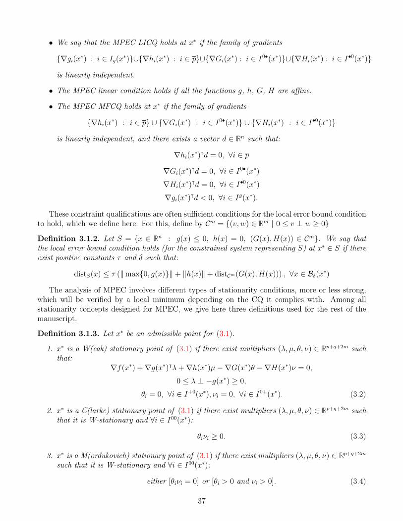
• We say that the MPEC LICQ holds at x∗ if the family of gradients
∇gi(x∗) : i ∈ Ig(x∗)∪∇hi(x∗) : i ∈ p∪∇Gi(x∗) : i ∈ I0•(x∗)∪∇Hi(x
∗) : i ∈ I•0(x∗)
is linearly independent.
• The MPEC linear condition holds if all the functions g, h, G, H are affine.
• The MPEC MFCQ holds at x∗ if the family of gradients
∇hi(x∗) : i ∈ p ∪ ∇Gi(x∗) : i ∈ I0•(x∗) ∪ ∇Hi(x
∗) : i ∈ I•0(x∗)
is linearly independent, and there exists a vector d ∈ Rn such that:
∇hi(x∗)ᵀd = 0, ∀i ∈ p
∇Gi(x∗)ᵀd = 0, ∀i ∈ I0•(x∗)
∇Hi(x∗)ᵀd = 0, ∀i ∈ I•0(x∗)
∇gi(x∗)ᵀd < 0, ∀i ∈ Ig(x∗).
These constraint qualifications are often sufficient conditions for the local error bound conditionto hold, which we define here. For this, define by Cm = (v, w) ∈ Rm | 0 ≤ v ⊥ w ≥ 0
Definition 3.1.2. Let S = x ∈ Rn : g(x) ≤ 0, h(x) = 0, (G(x), H(x)) ∈ Cm. We say thatthe local error bound condition holds (for the constrained system representing S) at x∗ ∈ S if thereexist positive constants τ and δ such that:
distS(x) ≤ τ (‖max0, g(x)‖+ ‖h(x)‖+ distCm(G(x), H(x))) , ∀x ∈ Bδ(x∗)
The analysis of MPEC involves different types of stationarity conditions, more or less strong,which will be verified by a local minimum depending on the CQ it complies with. Among allstationarity concepts designed for MPEC, we give here three definitions used for the rest of themanuscript.
Definition 3.1.3. Let x∗ be an admissible point for (3.1).
1. x∗ is a W(eak) stationary point of (3.1) if there exist multipliers (λ, µ, θ, ν) ∈ Rp+q+2m suchthat:
∇f(x∗) +∇g(x∗)ᵀλ+∇h(x∗)µ−∇G(x∗)θ −∇H(x∗)ν = 0,
0 ≤ λ ⊥ −g(x∗) ≥ 0,
θi = 0, ∀i ∈ I+0(x∗), νi = 0, ∀i ∈ I0+(x∗). (3.2)
2. x∗ is a C(larke) stationary point of (3.1) if there exist multipliers (λ, µ, θ, ν) ∈ Rp+q+2m suchthat it is W-stationary and ∀i ∈ I00(x∗):
θiνi ≥ 0. (3.3)
3. x∗ is a M(ordukovich) stationary point of (3.1) if there exist multipliers (λ, µ, θ, ν) ∈ Rp+q+2m
such that it is W-stationary and ∀i ∈ I00(x∗):
either [θiνi = 0] or [θi > 0 and νi > 0]. (3.4)
37
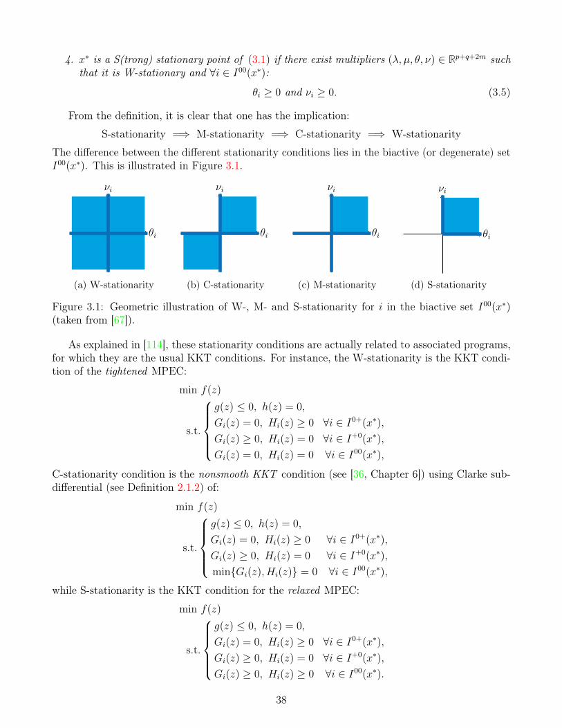
4. x∗ is a S(trong) stationary point of (3.1) if there exist multipliers (λ, µ, θ, ν) ∈ Rp+q+2m suchthat it is W-stationary and ∀i ∈ I00(x∗):
θi ≥ 0 and νi ≥ 0. (3.5)
From the definition, it is clear that one has the implication:
S-stationarity =⇒ M-stationarity =⇒ C-stationarity =⇒ W-stationarity
The difference between the different stationarity conditions lies in the biactive (or degenerate) setI00(x∗). This is illustrated in Figure 3.1.
θi
νi
(a) W-stationarity
θi
νi
(b) C-stationarity
θi
νi
(c) M-stationarity
θi
νi
(d) S-stationarity
Figure 3.1: Geometric illustration of W-, M- and S-stationarity for i in the biactive set I00(x∗)(taken from [67]).
As explained in [114], these stationarity conditions are actually related to associated programs,for which they are the usual KKT conditions. For instance, the W-stationarity is the KKT condi-tion of the tightened MPEC:
min f(z)
s.t.
g(z) ≤ 0, h(z) = 0,
Gi(z) = 0, Hi(z) ≥ 0 ∀i ∈ I0+(x∗),
Gi(z) ≥ 0, Hi(z) = 0 ∀i ∈ I+0(x∗),
Gi(z) = 0, Hi(z) = 0 ∀i ∈ I00(x∗),
C-stationarity condition is the nonsmooth KKT condition (see [36, Chapter 6]) using Clarke sub-differential (see Definition 2.1.2) of:
min f(z)
s.t.
g(z) ≤ 0, h(z) = 0,
Gi(z) = 0, Hi(z) ≥ 0 ∀i ∈ I0+(x∗),
Gi(z) ≥ 0, Hi(z) = 0 ∀i ∈ I+0(x∗),
minGi(z), Hi(z) = 0 ∀i ∈ I00(x∗),
while S-stationarity is the KKT condition for the relaxed MPEC:
min f(z)
s.t.
g(z) ≤ 0, h(z) = 0,
Gi(z) = 0, Hi(z) ≥ 0 ∀i ∈ I0+(x∗),
Gi(z) ≥ 0, Hi(z) = 0 ∀i ∈ I+0(x∗),
Gi(z) ≥ 0, Hi(z) ≥ 0 ∀i ∈ I00(x∗).
38

With the previous definitions, we can now state some first-order conditions for (3.1).
Theorem 3.1.1. 1. [95, Theorem 2 (1)] Let x∗ be a local optimal solution for (3.1), and supposeMPEC MFCQ holds at x∗. Then x∗ is C-stationary.
2. [114, Theorem 2.2] Suppose the MPEC linear CQ is met. Let x∗ be a local optimal solutionfor (3.1). Then x∗ is M-stationary.
3. [83, Theorem 3] Let x∗ be a local optimal solution for (3.1), and suppose MPEC LICQ holdat x∗. Then x∗ is S-stationary.
The definition of stationarities in Definition 3.1.3 uses some index sets that depend on theoptimal solution (namely, I+0(x∗) and all the other (bi)active sets). This dependence may some-times be cumbersome, and prevent the resolution of these stationary conditions directly. The nextTheorem reformulates them, in order to get rid of these index sets.
Theorem 3.1.2. [58, Theorem 3.1] For any x admissible for (3.1), we have the following state-ments:
1. Conditions (3.2) and (3.3) are equivalent to the equations
θiGi(x) = νiHi(x) = 0, θiνi ≥ 0, i ∈ m
2. Conditions (3.2) and (3.4) are equivalent to the equations
θiGi(x) = νiHi(x) = 0, θiνi ≥ 0, maxui, vi ≥ 0, i ∈ m
3. Conditions (3.2) and (3.5) are equivalent to the equations
θi = αi − ζHi(x), νi = βi − ζGi(x)
αiGi(x) = βiHi(x) = 0, αiβi ≥ 0, i ∈ m(3.6)
for α, β ∈ Rm and ζ ∈ R.
Remark 3.1.1. Concerning the reformulation of S-stationarity, one may see α and β as themultipliers associated with the constraints G(x) ≥ 0, H(x) ≥ 0, and ζ as the multiplier associatedwith the constraint G(x)ᵀH(x) = 0, where (3.1) is considered as a standard NLP. Since neitherthe (standard) LICQ nor MFCQ apply directly to these constraints, [110, Theorem 1] states thatthese multipliers (α, β, ζ) can not be unique, nor can they remain in a bounded set.
Other results related to this problem can be found in the aforementioned references and in[75, 82, 113].
3.1.2 Numerical resolution
Of course, most MPEC can not be solved analytically. In general, the numerical treatment ofMPEC is not an easy task. Due to the violation of standard CQs, most optimization solvers arenot guaranteed to converge. The algorithms designed for their resolution try to tackle this problemwhile focusing on two points:
• Of course, the algorithm has to converge to a local optimum, or at least to a stationary point.
• Preferably, it should fit in the already known algorithms used for classical optimization.
It should be noted also that there exists a benchmark with numerous MPEC problems and theirsolution, used for testing the different algorithms; see [72]. We present here two schemes that mayconverge to M- or S-stationary points.
39

Complementarity relaxation
In [67], the idea is to relax the complementarity condition using the following C-function (seeDefinition 1.1.1): define ϕ : R2 → R by:
ϕ(a, b) =
ab if a+ b ≥ 0
−12(a2 + b2) if a+ b < 0
and then relax the problem as: let Φ : Rn × R+ → Rm be defined component-wise by:
Φi(z, τ) = ϕ(Gi(z)− τ,Hi(z)− τ)
With this function, we define the relaxed problem NLP(τ) for τ ≥ 0 as:
min f(z)
s.t. g(z) ≤ 0, h(z) = 0
G(z) ≥ 0, H(z) ≥ 0
Φ(z, τ) ≤ 0
(NLP(τ))
Algorithm 1: Relaxation algorithm (z0, τ0, σ, τmin, ε).Input: A starting vector z0, an initial relaxation parameter τ0, and parameters σ ∈ (0, 1),
τmin > 0, and ε > 01 Set k:=02 while (τk ≥ τmin and compVio(zk) > ε) or k=0 do3 Find an approximate solution zk+1 of NLP(τk). To solve NLP(τk), use zk as starting
vector. If NLP(τk) is not feasible, terminate the algorithm4 Let τk+1 ← σminτk, compVio(zk+1) and k ← k + 1
5 endOutput: The final iterate zopt = zk, the corresponding function value f(zopt), and the
maximum constraint violation maxV io(zopt).In this algorithm, we denote:
compVio(z) = maxminGi(z), Hi(z), i ∈ m
maxVio(z) = maxmax0, gj(z), |hk(z)|, |minGi(z), Hi(z)|, j ∈ q, k ∈ p, i ∈ m
Theorem 3.1.3. [67, Theorem 4.1, 4.2] Let τk ↓ 0 and (zk, λk, µk, γk, νk, δk be a sequence ofKKT points of NLP(τk) with zk → z∗. If MPEC LICQ holds in z∗, then z∗ is an M-stationarypoint of the MPEC (3.1).Furthermore, if there is a subsequence K ⊆ N such that:
Gi(zk) ≤ τk, Hi(z
k) ≤ τk, ∀k ∈ K, ∀i ∈ I00(z∗)
then z∗ is a S-stationary point of (3.1).
However, it should be noted that this convergence is actually sensitive to instabilities.
40
Definition 3.1.4. Let ε > 0. We say that z∗ is an ε-stationary point of the problem
min f(z) s.t. g(z) ≤ 0, h(z) = 0
if there are multipliers λ and µ such that:
‖∇f(z∗) + (∇g(z∗))ᵀλ+ (∇h(z∗))ᵀµ‖∞ ≤ ε
g(z∗) ≤ 0, λ ≥ 0, λigi(z∗) ≥ −ε, ∀i
|hi(z∗)| ≤ ε, ∀i
Theorem 3.1.4. [67, Theorem 4.13] Let τk ↓ 0, εk = o(τk), and zk be a sequence of εk-stationarypoints of NLP(τk) with multipliers (λk, µk, γk, νk, δk). Assume that zk → z∗. If MPEC LICQ holdsat z∗, then z∗ is a W-stationary point of MPEC (3.1). Furthermore, if there is a subsequenceK ⊆ N such that:
Gi(zk) ≤ τk, Hi(z
k) ≤ τk, ∀k ∈ K, ∀i ∈ I00(z∗)
then z∗ is a C-stationary point of (3.1).
Cost penalization
The technique used in [73] is the penalization of the objective function. The complementarity ismoved to the objective function in the form of an `1-penalty term, so that the objective becomes:
f(z) + πG(z)ᵀH(z)
The associated barrier problem is defined as:
min f(z) + πG(z)ᵀH(z)− µ
(∑i
log si +∑i
logGi(z) +∑i
logHi(z)
)s.t. h(z) = 0
g(z)− s = 0
(3.7)
The Lagrangian of this barrier problem is given by:
Lµ,π(z, s, λ, θ) = f(z) + πG(z)ᵀH(z)− µ
(∑i
log si +∑i
logGi(z) +∑i
logHi(z)
)−∑i
θihi(z)−∑i
λi(gi(z)− si)
41
Algorithm 2: Classic: A Practical Interior-Penalty Method for MPECs.Input: Let z0, s0, λ0, θ0 be the initial value of the primal and dual variables.
1 Set k = 1.2 repeat3 Choose a barrier parameter µk, a stopping tolerance εkpen and εkcomp4 Find πk and an approximate solution (xk, sk, λk, θk) of problem (3.7) with parameter µk
and πk that satisfy G(zk) > 0, H(zk) > 0, sk > 0, λk > 0 and the following conditions:
‖∇zLµk,πk(zk, sk, λk, θk)‖ ≤ εkpen
‖ski λki − µk‖ ≤ εkpen, ∀i∥∥∥∥ h(zk)g(zk)− sk
∥∥∥∥ ≤ εkpen
‖minG(zk), H(zk)‖ ≤ εkcomp
5 Let k ← k + 1
6 until a stopping test for the MPEC is satisfied
Theorem 3.1.5. [73, Theorem 3.4 and Corollary 3.5] Suppose that Algorithm 2 generates aninfinite sequence of iterates zk, sk, λk, θk and parameters πk, µk, for sequences εkpen, εkcomp,µk converging to zero. If z∗ is a limit point of the sequence zk, and f , g and h are continuouslydifferentiable in an open neighborhood N (z∗) of z∗, then z∗ is feasible for (3.1). If in addition,MPEC LICQ holds at z∗, then z∗ is C-stationary. Moreover, if πk is bounded, then z∗ is anS-stationary point of (3.1).
3.2 Optimal controlRecently in [59], different results concerning MPEC have been adapted in order to analyze anOptimal Control problem with complementarity constraints:
min J(x, u) =
∫ T
0
F (t, x(t), u(t))dt+ f(x(0), x(T ))
s.t.
x(t) = φ(t, x(t), u(t))
g(t, x(t), u(t)) ≤ 0
h(t, x(t), u(t)) = 0
0 ≤ G(t, x(t), u(t)) ⊥ H(t, x(t), u(t)) ≥ 0
u(t) ∈ U(t)
a.e. t ∈ [0, T ]
(x(0), x(T )) ∈ E .
(3.8)
with F : [0, T ]×Rn×Rm → R, f : Rn×Rn → R, φ : [0, T ]×Rn×Rm → Rn, g : [0, T ]×Rn×Rm → Rq,h : [0, T ]× Rn × Rm → Rp, G,H : [0, T ]× Rn × Rm → Rl, U : [0, T ]⇒ Rm a multifunction, and Ea closed subset of R2n. This section will use different notions of normal cones and subdifferentials,which are defined in the Appendix A.
42
3.2.1 Necessary conditions
We suppose that F and φ are L × B-measurable, where L × B denotes the σ-algebra of subsetsof appropriate spaces generated by product sets M × N , where M is a Lebesgue (L) measurablesubset in R, and N is a Borel (B) measurable subset in Rn × Rm.
Definition 3.2.1. • We refer to any absolutely continuous function as an arc.
• An admissible pair for (3.8) is a pair of functions (x, u) on [0, T ] for which u is a controland x is an arc, that satisfy all the constraints in (3.8).
• The complementarity cone is defined by
Cm = (v, w) ∈ Rm | 0 ≤ v ⊥ w ≥ 0
• We define the set constraint at time t ∈ [0, T ], S(t), by:
S(t) = (x, u) ∈ Rn × U(t) : g(t, x, u) ≤ 0, h(t, x, u) = 0, (G(t, x, u), H(t, x, u)) ∈ Cm .
• We say that the local error bound condition holds (for the constrained system representing S)at (x∗, u∗) ∈ S if there exist positive constants τ and δ such that: ∀(x, u) ∈ Bδ(x∗, u∗)
distS(x, u) ≤ τ (‖max0, g(x, u)‖+ ‖h(x, u)‖+ distCl(G(x, u), H(x, u)))
• For every given t ∈ [0, T ] and two positive constants R and ε, we define a neighbourhood ofthe point (x∗(t), u∗(t)) as:
Sε,R∗ (t) = (x, u) ∈ S(t) : ‖x− x∗(t)‖ ≤ ε, ‖u− u∗(t)‖ ≤ R. (3.9)
(x∗, u∗) is a local minimizer of radius R if there exists ε such that for every pair (x, u)admissible for (3.8) such that:
(x(t), u(t)) ∈ Sε,R∗ (t), a.e. t ∈ [0, T ],
∫ T
0
‖x∗(t)− x(t)‖dt ≤ ε
we have J(x∗, u∗) ≤ J(x, u).
Assumption 3.2.1. (a) There exist measurable functions kφx , kFx , kφw, kFw such that for almostevery t ∈ [0, T ] and for every (x1, w1), (x2, w2) ∈ Sε,R∗ (t), we have:
(a) ‖φ(t, x1, w1)− φ(t, x2, w2)‖ ≤ kφx(t)‖x1 − x2‖+ kφw(t)‖w1 − w2‖(b) |F (t, x1, w1)− F (t, x2, w2)| ≤ kFx (t)‖x1 − x2‖+ kFw(t)‖w1 − w2‖.
(3.10)
(b) There exists a positive measurable function kS such that for almost every t ∈ [0, T ], thebounded slope condition holds:
(x,w) ∈ Sε,R∗ (t), (α, β) ∈ N PS(t)(x,w) =⇒ ‖α‖ ≤ kS(t)‖β‖. (3.11)
(c) The functions kφx , kFx and kS[kφw + kFw ] are integrable, and there exists a positive number ηsuch that R(t) ≥ ηkS(t) a.e. t ∈ [0, T ].
43
(d) F and φ are L × B-measurable, f is locally Lipschitz continuous, g, h, G and H are L-measurable in variable t and strictly differentiable in variable (x, u), f is locally Lipschitzcontinuous, and E is a closed subset in R2n. U is a L measurable multifunction with convexvalues.
Assumption 3.2.1(b) is the central in [46], but it is rarely trivial to check if a given systemcomplies with this assumption. As it is stated at the end of Section 2 in [46], this bounded slopecondition excludes unilateral state constraints; that is, constraints of the type x(t) ∈ X(t) (sincein this case, there exists normals of the form (α, 0) in (3.11)).
Define the setsI−t (x, u) = i ∈ q : gi(t, x(t), u(t)) < 0,
I+0t (x, u) = i : Gi(t, x(t), u(t)) > 0 = Hi(t, x(t), u(t)),
I0+t (x, u) = i : Gi(t, x(t), u(t)) = 0 < Hi(t, x(t), u(t)),
I00t (x, u) = i : Gi(t, x(t), u(t)) = 0 = Hi(t, x(t), u(t)),
and for any (λg, λh, λG, λH) ∈ Rq+p+m+m, denote:
Ψ(t, x, u;λg, λh, λG, λH) = g(t, x, u)ᵀλg + h(t, x, u)ᵀλh −G(t, x, u)ᵀλG −H(t, x, u)ᵀλH . (3.12)
Theorem 3.2.1. [59] Let (x∗, u∗) be a local minimizer of radius R for (3.8) and let Assumption3.2.1 hold. If for almost every t ∈ [0, T ] the local error bound condition for the system representingS(t) holds at (x∗(t), u∗(t)), then there exist a number λ0 ∈ 0, 1, an arc p and measurable functionsλg : R→ Rq, λh : R→ Rp, λG, λH : R→ Rm such that the following conditions hold:
1. the non-triviality condition: (λ0, p(t)) 6= 0, ∀t ∈ [0, T ]
2. the transversality condition:
(p(0),−p(T )) ∈ λ0∂Lf(x∗(0), x∗(T )) +NE (x∗(0), x(T )) (3.13)
3. the Euler adjoint inclusion: for almost every t ∈ [0, T ],
(p(t), 0) ∈ ∂C 〈−p(t), φ(t, ·, ·)〉+ λ0F (t, ·, ·) (x∗(t), u∗(t))
+∇x,uΨ(t, x∗(t), u∗(t);λg(t), λh(t), λG(t), λH(t))
+ 0 × NU(t)(u∗(t))
(3.14)
λg(t) ≥ 0, λgi (t) = 0, ∀i ∈ I−t (x∗, u∗)
λGi (t) = 0, ∀i ∈ I+0t (x∗(t), u∗(t)), λHi (t) = 0, ∀i ∈ I0+
t (x∗(t), u∗(t))
4. the Weierstrass condition for radius R: for almost every t ∈ [0, T ],
(x∗(t), u) ∈ S(t), ‖u− u∗(t)‖ < R(t)
=⇒ 〈p(t), φ(t, x∗(t), u)〉 − λ0F (t, x∗(t), u) ≤ 〈p(t), φ(t, x∗(t), u∗(t))〉 − λ0F (t, x∗(t), u∗(t))
44
The Weierstrass condition can be re-expressed as searching a local minimizer of the followingMPEC:
max 〈p(t), φ(t, x∗(t), u)〉 − λ0F (t, x∗(t), u)
s.t.
(G(t, x∗(t), u), H(t, x∗(t), u)) ∈ Cm
g(t, x∗(t), u) ≤ 0, h(t, x∗(t), u) = 0
(3.15)
where Cm is defined in Definition 3.2.1. For each t ∈ [0, T ], this is an MPEC which admitsstationarity conditions as exposed in Section 3.1.
Definition 3.2.2. Let (x∗, u∗) be an admissible pair for (3.8).
• The Fritz-John (FJ) type W-stationarity holds at (x∗, w∗) if there exist a number λ0 ∈ 0, 1,an arc p and measurable functions λG, λH such that Theorem 3.2.1 (1)-(4) hold.
• The FJ-type M-stationarity holds at (x∗, u∗) if (x∗, u∗) is W-stationarity with arc p and thereexist measurable functions ηg, ηh, ηG, ηH such that, for almost every t ∈ [0, T ],
0 ∈ ∂L 〈−p(t), φ(t, x∗(t), ·) + λ0F (t, x∗(t), ·) (u∗(t))
+∇uΨ(t, x∗(t), u∗(t); ηg(t), ηh(t), ηG(t), ηH(t)) +NU(t)(u∗(t))
ηg(t) ≥ 0, ηgi (t) = 0, ∀i ∈ I−t (x∗, u∗)
ηGi (t) = 0, ∀i ∈ I+0t (x∗(t), u∗(t)), ηHi (t) = 0, ∀i ∈ I0+
t (x∗(t), u∗(t))
either [ηGi (t)ηHi (t) = 0] or [ηGi (t) > 0 and ηHi (t) > 0], ∀i ∈ I00t (x∗(t), u∗(t)).
• The FJ-type S-stationarity holds at (x∗, u∗) if (x∗, u∗) is W-stationarity with arc p and thereexist measurable functions ηG, ηH such that, for almost every t ∈ [0, T ],
0 ∈ ∂L 〈−p(t), φ(t, x∗(t), ·) + λ0F (t, x∗(t), ·) (u∗(t))
+∇uΨ(t, x∗(t), u∗(t); ηg(t), ηh(t), ηG(t), ηH(t)) +NU(t)(u∗(t))
ηg(t) ≥ 0, ηgi (t) = 0, ∀i ∈ I−t (x∗, u∗)
ηGi (t) = 0, ∀i ∈ I+0t (x∗(t), u∗(t)), ηHi (t) = 0, ∀i ∈ I0+
t (x∗(t), u∗(t))
ηGi (t) ≥ 0, ηHi (t) ≥ 0, ∀i ∈ I00t (x∗(t), u∗(t)).
We refer to the FJ-type W-, M- and S-stationarities as the W-, M- and S-stationarities, respect-ively, if λ0 = 1.
Notice that we have now two different sets of multipliers, and as shown in [59, Example 3.4],these new multipliers ηG, ηH can be different in measure from the corresponding λG, λH . Non-etheless, the results concerning stationarity for MPEC still can be applied to (3.15):
Theorem 3.2.2. [59, Theorem 3.5] Let (x∗, u∗) be a local minimizer of radius R for (3.8), andlet Assumption 3.2.1 hold. Suppose also that the MPEC linear condition holds for S(t) for almostevery t ∈ [0, T ], i.e. functions g(t, ·, ·), h(t, ·, ·), G(t, ·, ·) and H(t, ·, ·) are affine and U(t) is aunion of finitely many polyhedral sets. Then the FJ-type M-stationarity holds at (x∗, u∗).
The difference between these two sets however vanishes if we further suppose that MPEC-LICQholds:
45

Theorem 3.2.3. [59] Let (x∗, u∗) be a local minimizer of radius R for (3.8), and let Assumption3.2.1 hold. If for almost every t ∈ [0, T ], the functions F (t, ·, ·) and φ(t, ·, ·) are strictly differentiableat (x∗(t), u∗(t)), and the MPEC LICQ holds at u∗(t) for problem (3.15), i.e., the family of gradients
∇ugi(t, x∗(t), u∗(t)) : i ∈ I0
t (x∗(t), u∗(t) ∪ ∇uh(t, x∗(t), u∗(t)) : i ∈ p∪∇uGi(t, x
∗(t), u∗(t)) : i ∈ I0•t (x∗(t), u∗(t)) ∪ ∇uHi(t, x
∗(t), u∗(t)) : i ∈ I•0t (x∗(t), u∗(t))
is linearly independent, where
I0t (x, u) = i ∈ q : gi(t, x(t), u(t)) = 0
I0•t (x∗(t), u∗(t)) = I0+
t (x∗(t), u∗(t)) ∪ I00t (x∗(t), u∗(t)),
I•0t (x∗(t), u∗(t)) = I+0t (x∗(t), u∗(t)) ∪ I00
t (x∗(t), u∗(t)),
then the FJ-type S-stationarity holds at (x∗, u∗). Moreover, the multipliers ηg, ηh, ηG, ηH can betaken as equal to λg, λh, λG, λH , respectively, almost everywhere.
3.2.2 Sufficient condition for the Bounded Slope Condition (3.11)The Bounded Slope Condition (3.11) is not an easy assumption to check. There are, however,some results that give sufficient conditions for it to hold. We give here two of them.
Proposition 3.2.1. [59] Assume that the local error bound condition holds at every (x, u) ∈ Sε,R∗ (t)and:
(x, u) ∈ Sε,R∗ (t), ζ ∈ N LU(t)(u),
λg ≥ 0, λgi = 0 ∀i ∈ I−t (x, u),
λGi = 0, ∀i ∈ I+0t (x, u), λHi = 0, ∀i ∈ I0+
t (x, u),
λGi > 0, λHi > 0, or λGi λHi = 0, ∀i ∈ I00
t (x, u)
=⇒ ‖∇xΨ(t, x, u;λg, λh, λG, λH)‖ ≤ kS(t)‖∇uΨ(t, x, u;λg, λh, λG, λH) + ζ‖,
where Ψ is defined in (3.12). Then the bounded slope condition (3.11) holds.
Let us define the following set:
Cε,R∗ = cl(t, x, u) ∈ [0, T ]× Rn × Rm : (x, u) ∈ Sε,R∗ (t)
Proposition 3.2.2. [59] Let the mappings g, h, G, H, U be autonomous. Assume that Cε,R∗ is
compact for some ε > 0, the local error bound holds, and that, for every (x, u) such that (t, x, u) ∈Cε,R, the system complies with the following implication:
0 ∈ ∇uΨ(t, x, u;λg, λh, λG, λH) +N LU(t)(u)
λg ≥ 0, λgi = 0 ∀i ∈ I−t (x, u),
λGi = 0, ∀i ∈ I+0t (x, u), λHi = 0, ∀i ∈ I0+
t (x, u),
λGi > 0, λHi > 0, or λGi λHi = 0, ∀i ∈ I00
t (x, u)
=⇒ ∇xΨ(t, x, u;λg, λh, λG, λH) = 0,
where Ψ is defined in (3.12). Then there exists a positive constant kS such that for every t ∈ [0, T ],the bounded slope condition (3.11) holds with kS(t) = kS.
46
Conclusion
This presentation of MPEC showed how specific is the study of such systems, and which tools areneeded to tackle them properly. These will enable us to tackle efficiently the optimal control ofLCS, both analytically and numerically, as shown in the following chapters.
47

Part II
Quadratic optimal control of LCS: the 1Dcomplementarity case
48

Chapter 4
First order conditions using Clarke’ssubdifferential
Abstract. The optimal control of LCS is first tackled when the complementarity is one dimen-sional. In this case, the system can be re-expressed as a Lipschitz dynamical system, and Clarke’sresults concerning the optimal control of such system is used. After that, the optimality conditionsare equivalently expressed in a different form. All these results are used to derive the analyticalsolution of a simple 1D class of problems. This Chapter has been published in [107].
We start the analysis of this problem with a simplified problem, with a complementarity whichis one dimensional:
x(t) = Ax(t) +Bλx(t) + Fu(t),0 ≤ λx(t) ⊥ Cx(t) + dλx(t) + eu(t) ≥ 0,x(0) = x0, x(T ) free
a.e. on [0, T ] (4.1)
where A ∈ Rn×n, B,F ∈ Rn, C ∈ R1×n, d, e ∈ R, d > 0, T > 0, x : [0, T ] → Rn is absolutelycontinuous, u : [0, T ] → R is square integrable, and λx : [0, T ] → R is measurable. In order toavoid trivial cases, we assume that (C, e) 6= (0, 0).
We define now the optimal control problem of finding the trajectories of (4.1) minimizing thefunctional:
C(x, u) =
∫ T
0
f 0(x(t), u(t))dt =
∫ T
0
(x(t)ᵀx(t) + u(t)2)dt. (4.2)
In this case, an optimal trajectory (x∗, u∗) is a W 1,1 local minimizer, meaning: there exists ε > 0such that, for any admissible trajectory for (4.1) (x, u) which verifies:
‖x− x∗‖W 1,1 =
∫ T
0
‖x(t)− x∗(t)‖dt ≤ ε
one has C(x∗, u∗) ≤ C(x, u).The reason to focus on this simplified problem is that basic convex analysis proves that λx(t) =
1dΠR+ (−Cx(t)− eu(t)), where ΠK(x) is the projection of x on the set K. Therefore, (4.1) becomes
(where the argument t is omitted for simplification):
x = fx(x, u),
= Ax+ Fu+B
dΠR+(−Cx− eu),
=
Ax+ Fu if Cx+ eu ≥ 0,(
A− BCd
)x+
(F − e
dB)u otherwise,
(4.3)
49
with obvious definition for fx. With this simple system, some first order conditions of optimalitywill be derived, that will show some advantages that LCS possess over other modeling paradigms.
4.1 Derivation of the maximum principle
4.1.1 Preliminary results
Remark that (4.3) is actually a Lipschitz differential equation, and the optimal control problem(4.1)(4.2) admits no further constraints. Therefore, we can use Theorem 2.1.1. It yields thefollowing result:
Proposition 4.1.1. Let (x∗, u∗) be a local minimizer. There exists an absolutely continuous func-tion p : [0, T ]→ Rn such that:
− p(t) ∈ fp(x∗(t), p(t), u∗(t)) = ∂Cx fx(x∗(t), u∗(t))p(t)− 1
2∂Cx f
0(x∗(t), u∗(t)), (4.4)
p(0) is free, and p(T ) = 0. It also complies with the Weierstrass condition:
〈fx(x∗(t), u∗(t)), p(t)〉 − 1
2f 0(x∗(t), u∗(t)) = sup
v∈Rm
〈fx(x∗(t), v), p(t)〉 − 1
2f 0(x∗(t), v)
(4.5)
Recall that ∂Cx denotes the Clarke subdifferential with respect to the x variable, defined in theAppendix A.
Proof. First, we need to define properly the set X in (2.4). As it has been remarked in [40, Remark4], X can depend on time as long as an ε-neighbourhood of x∗(t) lies in the interior of X(t). Letus define X(t) as an ε-neighbourhood of x∗(t) with ε big enough.Since x∗(T ) is free, it implies p(T ) = 0. We easily prove that the non-positive number λ appearingin Theorem 2.1.1 can not be 0 (since otherwise, |p(T )|+λ = 0). Therefore it can be chosen as −1
2.
The differential inclusion and the Weierstrass condition are just simple transcripts of the result.We just need to verify the hypotheses H1-H3. H1 and H3 are easily verified. Concerning H2(which asserts that the dynamical system is Lipschitz with respect to x), since fx and f 0 are bothlocally Lipschitz, and since X(t) is bounded for all t in [0, T ], the inequality trivially holds.
Let us compute these differential inclusions. Since f 0 is smooth, its subdifferential only containsthe gradient:
∂Cx f0(x, u) = 2x
Concerning the right-hand side of the dynamical system, its subdifferential is expressed as:
∂Cx fx(x, u) =
A if Cx+ eu > 0,
A− BCd
if Cx+ eu < 0,[
A− BCd, A]
if Cx+ eu = 0.
using the notation:[M1,M2] = convM1,M2
for any pair (M1, M2) of according dimensions matrices and where convM1,M2 stands for theconvex hull of M1 and M2.
50
Therefore, (4.4) becomes:
− p(t) ∈
−x(t) + Aᵀp(t) if Cx+ eu > 0,−x(t) +
(A− BC
d
)ᵀp(t)
if Cx+ eu < 0,
−x(t)+[(A− BC
d
)ᵀ, Aᵀ
]p(t) if Cx+ eu = 0.
(4.6)
In order to compute an optimal control, the system should obviously be controllable betweenthe initial and final points. We will only focus on completely controllable systems, relying onTheorem 1.2.3 stating the complete controllability of some LCS.
4.1.2 Equations (4.1) and (4.6) as a mixed LCS (MLCS)
We denote z =
(xp
). Let us rewrite (4.1) and (4.6) in the compact form:
z ∈(fx(z, u)fp(z, u)
)(4.7)
where the right-hand side is a set-valued function defined by:
• if Cx+ eu > 0: (fx(z, u)fp(z, u)
)=
(Ax+ Fux− Aᵀp
),
• if Cx+ eu < 0: (fx(z, u)fp(z, u)
)=
((A− CB
d
)x+
(F − e
dB)u
x+(CᵀBᵀ
d− Aᵀ
)p
),
• if Cx+ eu = 0: (fx(z, u)fp(z, u)
)=
( (A− FC
e
)x
x+[CᵀBᵀ
d− Aᵀ,−Aᵀ
]p
).
We can recast the differential inclusion (4.7) in the framework of complementarity systems withlinear dynamics:
z =
(gx(z, u)gp(z, u)
)=
(A 0I −Aᵀ
)z +
(B 00 CᵀBᵀ
d
)(λx
λp1
)+
(F0
)u, (4.8)
0 ≤ λx ⊥ Cx+ dλx + eu ≥ 0, (4.9a)
0 ≤ |λpj1 | ⊥ Cx+ eu+ |Cx+ eu| ≥ 0, (4.9b)
0 ≤ |λpj2 | ⊥ |Cx+ eu| − (Cx+ eu) ≥ 0 j = 1...n, (4.9c)
|λpj1 |+ |λpj2 | = |pj| j = 1...n, (4.9d)
λp1 + λp2 = p, (4.9e)
where the subscript j denotes the j-th component of a vector, and λpi = (λp1i , ..., λpnn )ᵀ.
Proposition 4.1.2. The right-hand side of (4.7) is the same as the right-hand side of (4.8) definedwith the complementarity conditions in (4.9).
51
Proof. The first line (4.9a) gives obviously the same right-hand side as in the second line of (4.1),which is fx(z, p). Then, fx(z, u) = gx(z, u). Therefore, we have to check that the other lines in(4.9) are the same as in (4.6). To do so, we have to distinguish 3 cases:
• if Cx+ eu > 0, then from (4.9b), we deduce that λp1 = 0. It follows that:
gp(z, u) = x− Aᵀp = fp(z, u).
• if Cx + eu < 0, then from (4.9c), λ2p = 0, and therefore from (4.9e), λp1 = p. We then have
the following equality:
gp(z, u) = x+
(CᵀBᵀ
d− Aᵀ
)p = fp(z, u).
• if Cx + eu = 0, then from (4.9d), we have that |λpj1 | + |λpj2 | = |pj|, so that λpji ∈ [−pj, pj],
i = 1, 2, j = 1, ...n. But, in order to comply with the last equality (4.9e), we must haveλpji ∈ [0, 1]pj, i = 1, 2, j = 1, ..., n, and hence, λpi ∈ [0, 1]p, i = 1, 2. This gives us
gp(z, u) = x− Aᵀp+ [0, 1]CᵀBᵀ
dp
= x+
[CᵀBᵀ
d− Aᵀ,−Aᵀ
]p
= fp(z, u).
We can still have an even more interesting form of (4.9) by noticing that the function | · | ispiecewise linear and so, admits a representation in the form of an LCP. This is the topic of thenext lemma:
Lemma 4.1.1. Define 1n = (1, ..., 1)ᵀ ∈ Rn. The multipliers λx and λp1 given by system (4.9) areequally defined by the following system:
0 ≤ λx ⊥ Cx+ dλx + eu ≥ 00 ≤ µx,u ⊥ µx,u − 2(Cx+ eu) ≥ 00 ≤ µp ⊥ µp − 2p ≥ 00 ≤ λabs1 ⊥ µx,u1n ≥ 00 ≤ λabs2 ⊥ (µx,u − 2(Cx+ eu))1n ≥ 00 ≤ µ1 ⊥ µ1 − 2λp1 ≥ 00 ≤ µ2 ⊥ µ2 − 2λp2 ≥ 0
λabs1 + λabs2 = µp − pλp1 + λp2 = pµ1 − λp1 = λabs1
µ2 − λp2 = λabs2
(4.10)
where (4.10) is a mixed LCP (MLCP).
52
Proof. First, we need to establish the following simple result: for any scalar x, |x| = µ− x whereµ is given by:
0 ≤ µ ⊥ µ− 2x ≥ 0.
Indeed, if x ≤ 0, then we must take µ = 0, so that µ− x = −x = |x|. If x > 0, then we musttake µ = 2x, and µ− x = x = |x|. Let us use (4.9) to rewrite equivalently the absolute values as:
0 ≤ µx,u ⊥ µx,u − 2(Cx+ eu) ≥ 0,
0 ≤ µ1 ⊥ µ1 − 2λp1 ≥ 0,
0 ≤ µ2 ⊥ µ2 − 2λp2 ≥ 0,
0 ≤ µp ⊥ µp − 2p ≥ 0,
λabsx,u = µx,u − (Cx+ eu) = |Cx+ eu|,λabs1 = µ1 − λp1 = |λp1|,λabs2 = µ2 − λp2 = |λp2|,λabsp = µp − pᵀ = |p|,
where notation |x| on a vector x is here understood component-wise, e.g. |x| = (|x1|, ..., |xn|)ᵀ.Therefore, (4.9) becomes:
0 ≤ λx ⊥ Cx+ dλx + eu ≥ 00 ≤ µx,u ⊥ µx,u − 2(Cx+ eu) ≥ 00 ≤ µ1 ⊥ µ1 − 2λp1 ≥ 00 ≤ µ2 ⊥ µ2 − 2λp2 ≥ 00 ≤ µp ⊥ µp − 2p ≥ 00 ≤ λabs1 ⊥ (Cx+ eu+ λabsx,u)1n ≥ 00 ≤ λabs2 ⊥ (λabsx,u − (Cx+ eu))1n ≥ 0
λabs1 + λabs2 = λabspλp1 + λp2 = p
λabsx,u = µx,u − (Cx+ eu)λabs1 = µ1 − λp1λabs2 = µ2 − λp2λabsp = µp − p
Noticing that we can use the two equalities on λabsx,u and λabsp and insert them above, we haveproven that λx and λp1 are equally defined by (4.9) or (4.10).
Therefore, we infer that the right-hand side of the differential inclusion in (4.7) is equal to theright-hand side of system (4.8):
z = Az + BΛ + F u, (4.11)
where A, B, F and Λ are easily identifiable from (4.8), and subject to the MLCP (4.10).
53
4.2 Analytical solution for a 1D exampleThis result can be used in order to find the unique stationary trajectory of a special class of LCS.Suppose in (4.1) that n = 1 and C = 0; it means we try to tackle the following problem:
minimize∫ T
0
(x(t)2 + u(t)2
)dt,
such that:
x(t) = ax(t) + bλ(t) + fu(t),
0 ≤ λ(t) ⊥ dλ(t) + eu(t) ≥ 0, a.e. on [0, T ]
x(0) = x0, x(T ) free,
(4.12)
where all variables are scalar, d > 0, b, e 6= 0.
4.2.1 Complete controllability conditions for this 1D example
In order to analyze this problem, we will first specify the necessary and sufficient complete con-trollability conditions in the 1D case. Applying Theorem 1.2.3, we must check that the followingsystem:
(a− λ)ζ = 0, (4.13)fζ + eη = 0, (4.14)
η ≥ 0, (4.15)bζ + dη ≤ 0, (4.16)
has no solution λ ∈ R and (ζ, η) 6= 0
If e > 0: we deduce through (4.14): η = −fζe.
1. If f = 0, then η = 0. In (4.13), we can take λ = a. However, with (4.16), we have thatζb ≤ 0. Let us take ζ = −sign(b). Then we found a solution with ζ 6= 0: the system isnot completely controllable.
2. If f < 0, then with (4.15), we have that ζ ≥ 0. Through (4.13), we take λ = a.• If b ≥ 0, then (4.16) is a sum of positive terms which must be nonpositive, so η = 0
and ζ = 0: the system is completely controllable.• If b < 0, then (4.16) becomes ζ(b− fd
e) ≤ 0 with ζ ≥ 0.
– If b − fde≤ 0 then we can take any ζ ≥ 0: the system is not completely
controllable.– Otherwise, only ζ = 0 suits, so η = 0, and then the system is completely controllable.
3. If f > 0, then in (4.13), we take λ = a. Through (4.15), we have that ζ ≤ 0.• If b ≤ 0, then (4.16) is a positive terms sum which must be nonpositive, so η = 0
and ζ = 0: the system is completely controllable.• If b > 0, then (4.16) becomes ζ(b− fd
e) ≤ 0 with ζ ≤ 0.
– If b − fde≥ 0 then then we can take any ζ ≤ 0: the system is not completely
controllable.– Otherwise, only ζ = 0 suits, so η = 0, and then the system is completely controllable.
If e < 0: we have the same cases as with e > 0 by inverting the sign of f .
54
4.2.2 Search for the explicit optimal solution
The dynamic system in (4.12) can be rewritten as:
x = ax+ fu+b
dΠR+(−eu). (4.17)
Therefore, the Hamiltonian function is written as:
H(x, p, u) = p
(ax+ fu+
b
dΠR+(−eu)
)− 1
2
(x2 + u2
). (4.18)
We notice that this equation is smooth in x. Therefore, using (4.6), the adjoint equation issmooth, and is written as:
p(t) = −ap(t) + x(t).
We can even differentiate twice p, and obtain the following second-order differential equation:
p = −ap+ x
= a2p+ fu+b
dΠR+(−eu)
=
a2p+ fu if eu ≥ 0
a2p+(f − be
d
)u if eu ≤ 0.
We now search for an expression of the optimal control u∗, function of x and p, maximizing theHamiltonian function H(x, p, u∗). To that aim, we use the subdifferential of H with respect to u,written ∂CuH(x, p, u), and the fact that if u∗ maximizes H, then
0 ∈ ∂CuH(x, p, u∗).
In our problem, the subdifferential is written as
∂CuH(x, p, u) =
fp− u if eu > 0,(f − eb
d
)p− u
if eu < 0,
−[f − eb
d, f]p if eu = 0.
We now only focus on the complete controllable cases in order to find a control u maximizing thisfunction:
If e > 0: In that case, sgn(eu) =sgn(u).
1. We consider first f < 0.
• If b > 0, then if p ≤ 0, then fp ≥ 0,(f − eb
d
)p ≥ 0, and if p ≥ 0, then fp ≤ 0,(
f − ebd
)p ≤ 0. We also notice that 0 6∈
[f, f − eb
d
]. So we have:
u∗ =
fp if p ≤ 0,(f − eb
d
)p if p ≥ 0.
55

• If b < 0, then we must make sure that f < ebd. We notice that in this case,
0 6∈[f, f − eb
d
]. We are then in the exact same case as the previous one, and
therefore, the control is expressed the same way:
u∗ =
fp if p ≤ 0,(f − eb
d
)p if p ≥ 0.
2. We consider now f > 0.
• If b < 0, then if p ≤ 0, then fp ≤ 0,(f − eb
d
)p ≤ 0, and if p ≥ 0, then fp ≥ 0,(
f − ebd
)p ≥ 0. We also notice that 0 6∈
[f, f − eb
d
]. So we have:
u∗ =
fp if p ≥ 0,(f − eb
d
)p if p ≤ 0.
• If b > 0, then we must make sure that f > ebd. We notice that in this case,
0 6∈[f, f − eb
d
]. We are then in the exact same case as the previous one, and
therefore, the control is expressed the same way:
u∗ =
fp if p ≥ 0,(f − eb
d
)p if p ≤ 0
.
If e < 0: we have the same cases as with e > 0 by inverting the sign of f .
Therefore, we can summarize this result as follows:
u∗ =
fp if efp ≥ 0,(f − eb
d
)p if efp ≤ 0.
(4.19)
Finally, we use the optimal control found in (4.19) in the equation found on p. Surprisingly,we end up with a rather simple equation:
p =
(a2 + f 2) p if efp ≥ 0,(a2 +
(f − be
d
)2)p if efp ≤ 0,
which we rewrite in the more simple form:
p = γ(p)p (4.20)
with γ(p) > 0 and piecewise constant.We need now to find p(0) such that p(T ) = 0 (since x(T ) is free, according to the maximum
principle). Moreover, we know that the initial value for the derivative p is given by:
p(0) = x(0)− ap(0)
The phase portrait is depicted in Figure 4.1.
56
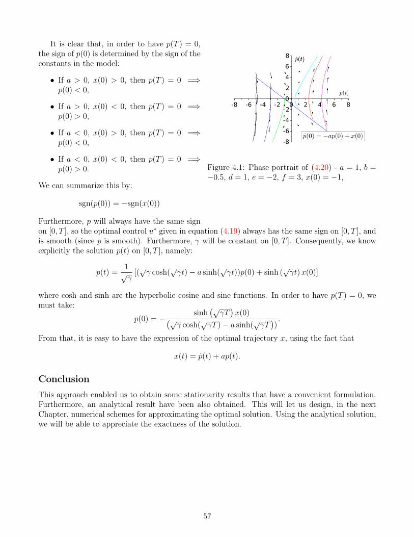
Figure 4.1: Phase portrait of (4.20) - a = 1, b =−0.5, d = 1, e = −2, f = 3, x(0) = −1,
It is clear that, in order to have p(T ) = 0,the sign of p(0) is determined by the sign of theconstants in the model:
• If a > 0, x(0) > 0, then p(T ) = 0 =⇒p(0) < 0,
• If a > 0, x(0) < 0, then p(T ) = 0 =⇒p(0) > 0,
• If a < 0, x(0) > 0, then p(T ) = 0 =⇒p(0) < 0,
• If a < 0, x(0) < 0, then p(T ) = 0 =⇒p(0) > 0.
We can summarize this by:
sgn(p(0)) = −sgn(x(0))
Furthermore, p will always have the same signon [0, T ], so the optimal control u∗ given in equation (4.19) always has the same sign on [0, T ], andis smooth (since p is smooth). Furthermore, γ will be constant on [0, T ]. Consequently, we knowexplicitly the solution p(t) on [0, T ], namely:
p(t) =1√γ
[(√γ cosh(
√γt)− a sinh(
√γt))p(0) + sinh (
√γt)x(0)]
where cosh and sinh are the hyperbolic cosine and sine functions. In order to have p(T ) = 0, wemust take:
p(0) = −sinh
(√γT)x(0)(√
γ cosh(√γT )− a sinh(
√γT)).
From that, it is easy to have the expression of the optimal trajectory x, using the fact that
x(t) = p(t) + ap(t).
Conclusion
This approach enabled us to obtain some stationarity results that have a convenient formulation.Furthermore, an analytical result have been also obtained. This will let us design, in the nextChapter, numerical schemes for approximating the optimal solution. Using the analytical solution,we will be able to appreciate the exactness of the solution.
57
Chapter 5
Numerical simulations
Abstract. Three numerical schemes are presented here: one which is a naive Direct method,and two other Indirect methods, based on the optimality condition derived in Chapter 4. Thanksto the analytical solution on which these schemes are tested, the correctness of the solutions isillustrated. This Chapter has been published in [107].
Obviously, there is little hope to solve analytically all possible problems of the form (4.1)(4.2).Therefore, some numerical schemes are designed in order to obtain a numerical approximations.Following the presentation of Section 2.2, we present here two numerical methods in order toapproximate the solution of (4.1)(4.2): a direct method, and an indirect method.
5.1 Numerical schemes
5.1.1 Direct method
A first way to solve the optimal problem is to discretize directly the dynamics (4.1) and the cost(4.2) in order to obtain a constrained optimization problem. In fact, a simple discretization thatwe can use here is the following one:
minu∈RN
N∑i=0
f 0(xi, ui),
s.t.
0 ≤ λxk ⊥ Cxk+1 + dλxk + euk ≥ 0xk+1−xk
h= Axk+1 +Bλxk + Fuk
k = 0...N − 1,
where the subscript k in zk denotes the k-th step in the discretization of the variable z(t) at timetk, and h denotes the (here uniform) time-step. Moreover, we can choose to integrate the dynamicswith an implicit (as presented here) or an explicit method. This is a Mathematical Program (MP)constrained by a Mixed Linear Complementarity Problem with parameters (G(·, u, ·), H(·, u, ·))where G : Rn(N+1) × RN+1 × RN+ → RnN and H : Rn(N+1) × RN+1 × RN+ → RN are definedcomponent-wise by:
Gk(x, u, λ) =xk+1 − xk
h− Axk+1 −Bλxk − Fuk,
Hk(x, u, λ) = Cxk+1 + dλxk + euk,
58
k = 0, ..., N − 1. We notice that we can isolate xk+1 in the dynamics, and reintroduce it in thecomplementarity conditions:
0 ≤ λxk ⊥ (d+ hC(I − hA)−1B)λxk + (e+ hC(I − hA)−1F )uk + C(I − hA)−1xk ≥ 0
5.1.2 Indirect method
A second way to compute an approximate solution of the optimal control problem is to discretize(4.11) under the constraints (4.10) and with the condition (4.5). This method is known as theindirect method (since it is using an a priori study of the system, and the result obtained with thePontryagin equations). Obviously, the choice of the discretization will eventually have an impacton the accuracy and the stability of the numerical solution. So as to have a first idea of the extentof these issues, these equations are discretized with an Euler scheme which will use implicit orexplicit terms in its formulation, and we will investigate how these choices affect the solution. Wepresent two formulations, that we name of explicit and implicit type. As we will see, these twoformulations lead to different types of optimization problems.
Explicit type
This first formulation leads to a problem where we can identify two (almost) independent problemsat each step. Let us assume we already know variables values of x and p at time tk, e.g. zk, andwe want to compute the solution at time tk+1. We first solve the following discretization of (4.5)with (4.10):
maxv∈R〈pk, fx(xk, v)〉+ p0f 0(xk, v),
s.t.
0 ≤ λxk ⊥ Cxk + dλxk + ev ≥ 00 ≤ µx,u ⊥ µx,u − 2(Cxk + ev) ≥ 00 ≤ µp ⊥ µp − 2pk ≥ 00 ≤ λabs1 ⊥ µx,u1n ≥ 00 ≤ λabs2 ⊥ (µx,u − 2(Cxk + ev))1n ≥ 00 ≤ µ1 ⊥ µ1 − 2λp1k ≥ 00 ≤ µ2 ⊥ µ2 − 2λp2k ≥ 0
λabs1 + λabs2 = µp − pkλp1k + λp2k = pkµ1 − λp1k = λabs1
µ2 − λp2k = λabs2
Solving this problem will give us uk and the associated Λk, which is unique for a given uk as wehave seen from the derivation of system (4.10), except in the case where Cxk + euk = 0. We canrewrite the complementarity conditions of this MPEC in the following compact form :
0 ≤ Ωk ⊥ ∆Ωk + Ψ ≥ 0
59
where Ωk = (λxk, µx,u, µp, λabs1 , λabs2 , µ1, µ2)ᵀ,
∆ =
d 0 0 0 0 0 00 1 0 0 0 0 00 0 1n 0 0 0 00 1n 0 0 0 0 00 1n 0 0 0 0 00 0 0 0 0 1n 00 0 0 0 0 0 1n
(5.1)
and Ψ is easily identifiable. Finally, we just need to integrate the dynamics (4.11), which isintegrated with the following discretization:
zk+1 − zkh
= Azk+1 + BΛk + F uk.
Here again, we can use an implicit integration, or an explicit one by introducing zk instead of zk+1
in the right-hand side.
Implicit type
This second formulation is expressed in the form of a single MPEC solved at each timestep. Here,every variable will be used implicitly, as the dynamics is introduced inside the constraints of theMP. Namely, we need to solve at each step the following MPEC:
maxv∈R〈pk+1, f(xk+1, v)〉+ p0f 0(xk+1, v)
s.t.
0 ≤ λxk+1 ⊥ Cxk+1 + dλxk+1 + ev ≥ 00 ≤ µx,u ⊥ µx,u − 2(Cxk+1 + ev) ≥ 00 ≤ µp ⊥ µp − 2pk+1 ≥ 00 ≤ λabs1 ⊥ µx,u1n ≥ 00 ≤ λabs2 ⊥ (µx,u − 2(Cxk+1 + ev))1n ≥ 00 ≤ µ1 ⊥ µ1 − 2λp1k+1 ≥ 00 ≤ µ2 ⊥ µ2 − 2λp2k+1 ≥ 0
λabs1 + λabs2 = µp − pk+1
λp1k+1 + λp2k+1 = pk+1
µ1 − λp1k+1 = λabs1
µ2 − λp2k+1 = λabs2zk+1−zk
h= Azk+1 + BΛk+1 + F v
5.2 Numerical results
5.2.1 Direct method
Consider the system given in (4.12). The direct method gives good, whatever the parametersused. We used the solver GAMS (available at http://www.gams.com/) which includes a powerfulMPEC solver. The only trouble noticed was that some fluctuations around the analytical solutionwere found (see Figure 5.1 for t ∈ [0.5, 1]), thus the results were difficult to achieve thin precision.Nonetheless, these fluctuations are still admissible in all the calculations we made. Some results areshown in Figure 5.1. The numerical performance of the direct method (including curves showingits order) are further extended in Section 7.1.
60
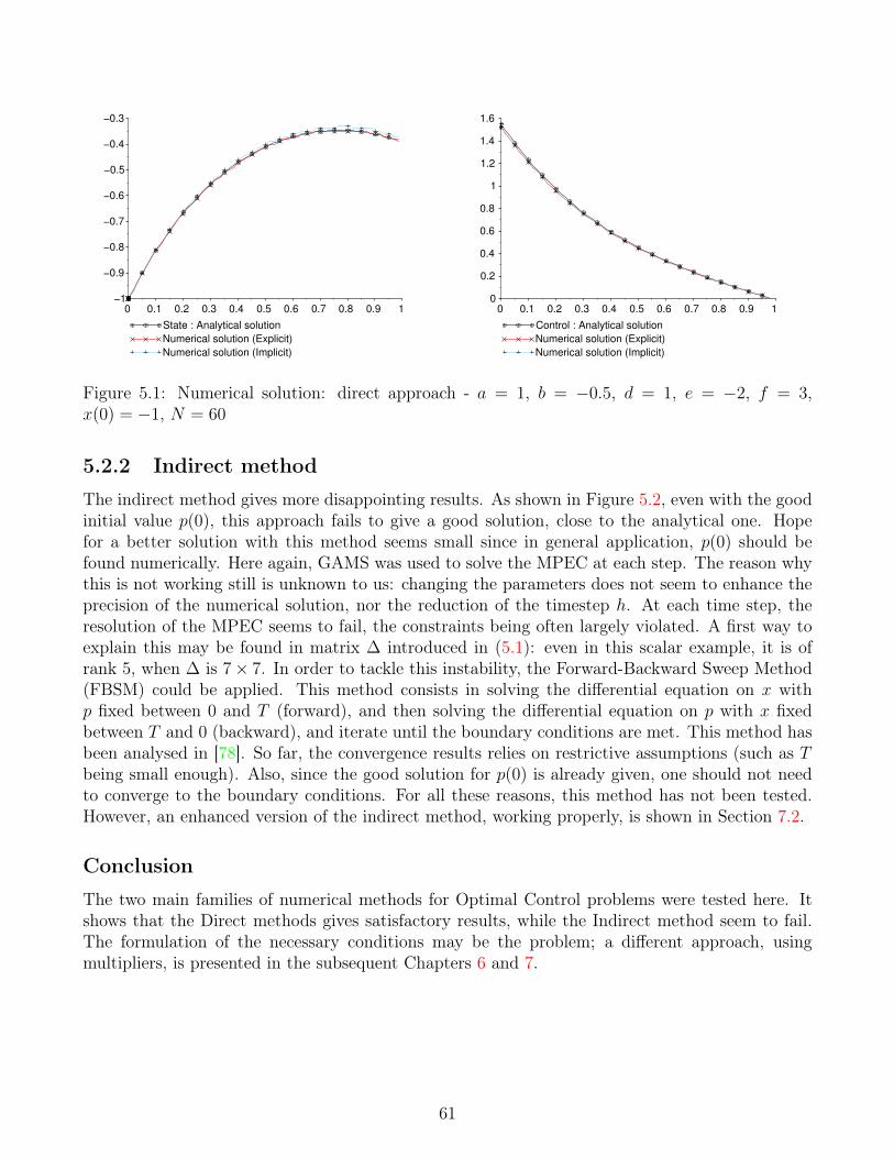
0 10.2 0.4 0.6 0.80.1 0.3 0.5 0.7 0.9−1
−0.8
−0.6
−0.4
−0.9
−0.7
−0.5
−0.3
State : Analytical solution
Numerical solution (Explicit)
Numerical solution (Implicit)
0 10.2 0.4 0.6 0.80.1 0.3 0.5 0.7 0.90
1
0.2
0.4
0.6
0.8
1.2
1.4
1.6
Control : Analytical solution
Numerical solution (Explicit)
Numerical solution (Implicit)
Figure 5.1: Numerical solution: direct approach - a = 1, b = −0.5, d = 1, e = −2, f = 3,x(0) = −1, N = 60
5.2.2 Indirect method
The indirect method gives more disappointing results. As shown in Figure 5.2, even with the goodinitial value p(0), this approach fails to give a good solution, close to the analytical one. Hopefor a better solution with this method seems small since in general application, p(0) should befound numerically. Here again, GAMS was used to solve the MPEC at each step. The reason whythis is not working still is unknown to us: changing the parameters does not seem to enhance theprecision of the numerical solution, nor the reduction of the timestep h. At each time step, theresolution of the MPEC seems to fail, the constraints being often largely violated. A first way toexplain this may be found in matrix ∆ introduced in (5.1): even in this scalar example, it is ofrank 5, when ∆ is 7× 7. In order to tackle this instability, the Forward-Backward Sweep Method(FBSM) could be applied. This method consists in solving the differential equation on x withp fixed between 0 and T (forward), and then solving the differential equation on p with x fixedbetween T and 0 (backward), and iterate until the boundary conditions are met. This method hasbeen analysed in [78]. So far, the convergence results relies on restrictive assumptions (such as Tbeing small enough). Also, since the good solution for p(0) is already given, one should not needto converge to the boundary conditions. For all these reasons, this method has not been tested.However, an enhanced version of the indirect method, working properly, is shown in Section 7.2.
Conclusion
The two main families of numerical methods for Optimal Control problems were tested here. Itshows that the Direct methods gives satisfactory results, while the Indirect method seem to fail.The formulation of the necessary conditions may be the problem; a different approach, usingmultipliers, is presented in the subsequent Chapters 6 and 7.
61
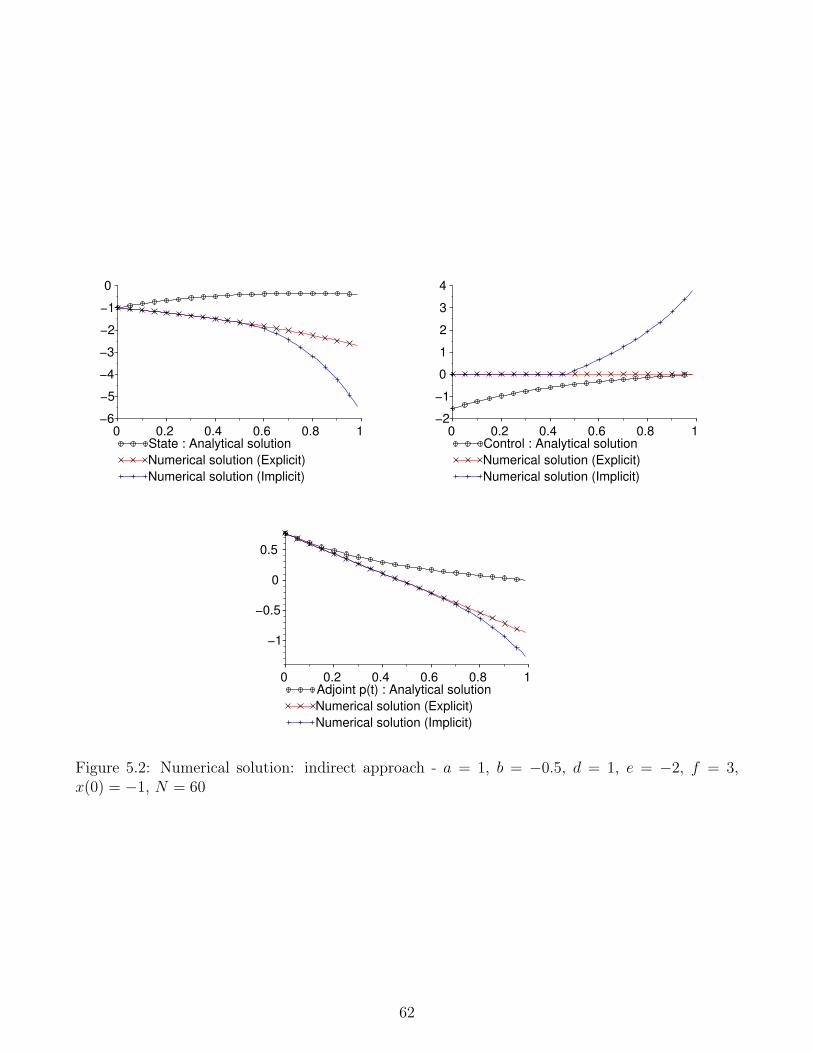
0 10.2 0.4 0.6 0.8
0
−6
−4
−2
−5
−3
−1
State : Analytical solution
Numerical solution (Explicit)
Numerical solution (Implicit)
0 10.2 0.4 0.6 0.8
0
−2
2
4
−1
1
3
Control : Analytical solution
Numerical solution (Explicit)
Numerical solution (Implicit)
0 10.2 0.4 0.6 0.8
0
−1
−0.5
0.5
Adjoint p(t) : Analytical solution
Numerical solution (Explicit)
Numerical solution (Implicit)
Figure 5.2: Numerical solution: indirect approach - a = 1, b = −0.5, d = 1, e = −2, f = 3,x(0) = −1, N = 60
62

Part III
Quadratic optimal control of LCS: thegeneral case
63
Chapter 6
Derivation of the first order conditions
Abstract. In this chapter, we will derive necessary conditions for the quadratic optimal controlof a general class of LCS. The first results involve index sets that are not convenient. Theseconditions are therefore re-expressed in the form of an LCS. In a second part, we will also showthat the weakest form of stationarity is actually a sufficient condition for optimality. This chapterhas been submitted to IEEE Transactions on Automatic Control [108].
The objective of this chapter is to analyze the quadratic optimal control of LCS. More precisely,we wish to investigate properties and numerical resolution of the problem:
min J(x, u, v) =
∫ T
0
(x(t)ᵀQx(t) + u(t)ᵀUu(t) + v(t)ᵀV v(t)) dt, (6.1)
subject to
x(t) = Ax(t) +Bv(t) + Fu(t),w(t) = Cx(t) +Dv(t) + Eu(t),0 ≤ v(t) ⊥ w(t) ≥ 0,Mx(0) +Nx(T ) = xb,
(6.2)
where T > 0, A,Q ∈ Rn×n, V,D ∈ Rm×m, U ∈ Rmu×mu , E ∈ Rm×mu , B ∈ Rn×m, F ∈ Rn×mu ,C ∈ Rm×n, M,N ∈ R2n×n, x : [0, T ] → Rn, u, v : [0, T ] → Rm, xb ∈ R2n. In order to avoid trivialcases, we assume that (C,E) 6= (0, 0) and xb is in the image set of (M N). Also, we choose Usymmetric and positive-definite, and Q and V semi-positive definite.
The problem of existence of solutions of the Optimal Control Problem (6.1)(6.2) is actuallytwofold. First, the existence of a trajectory for the LCS (6.2) is not straightforward, even ifthe system is expressed as an Initial Value Problem (IVP), as it was explained in Section 1.2.Secondly and most importantly, the existence of solution for (6.1)(6.2) is still an open question.A famous result due to Filipov [34, Theorem 9.2i] states the existence of an optimal controlunder convexity of the so-called velocity set V(x). In our case, V(x) = (u, v) ∈ R2m|0 ≤ v ⊥Cx+Dv + Eu ≥ 0 is clearly not convex, due to the complementarity. Therefore throughout thischapter, we admit that an optimal solution exists (in the sense of Definition 6.1.2 below), and thefocus is on necessary conditions this optimal solution must comply with (relying strongly on theseminal work in [59], presented in Section 3.2), together with their numerical computation whichrelies on MPEC algorithms (see Section 3.1.2).
This section uses normal cones that are defined in the Appendix A.
64
6.1 First-order necessary conditions for the optimal controlproblem (6.1)(6.2)
6.1.1 Preliminaries
Let us begin by recalling some definitions given in Sections 3.1 and 3.2 and particularized for theproblem (6.1)(6.2). First, let us fix some notations and definitions related to MPEC:
Definition 6.1.1. Let m ∈ N.
• The complementarity cone is defined as Cm = (v, w) ∈ Rm × Rm : 0 ≤ v ⊥ w ≥ 0.
• Three different index sets are defined from this complementarity constraint, called the activesets and the degenerate set:
I+0(v, w) = i ∈ m : v > 0 = w,
I0+(v, w) = i ∈ m : v = 0 < w,
I00(v, w) = i ∈ m : v = 0 = w.
The sets I•0(v, w) and I0•(v, w) are defined as I•0(v, w) = I+0(v, w) ∪ I00(v, w), I0•(v, w) =I0+(v, w) ∪ I00(v, w).
Definition 6.1.2. Let n,m,mu ∈ N.
• We refer to any absolutely continuous function on [0, T ] as an arc, and to any measurablefunction on [0, T ] as a control.
• An admissible pair for (6.2) is a 3-tuple of functions (x, u, v) on [0, T ] for which u, v arecontrols and x is an arc, that satisfy all the constraints in (6.2).
• Let us define the constraint set S, by
S = (x, u, v) ∈ Rn × Rmu × Rm : (v, Cx+Dv + Eu) ∈ Cm .
• Given a constant R > 0, we say that an admissible pair (x∗, u∗, v∗) is a local minimizerof radius R for (6.1)(6.2) if there exists ε > 0 such that for every pair (x, u, v) admissiblefor (6.2), which also satisfies ‖x(t) − x∗(t)‖ ≤ ε,
∥∥∥(uv)− (u∗(t)v∗(t)
)∥∥∥ ≤ R a.e. t ∈ [0, T ] and∫ T0‖x(t)− x∗(t)‖dt ≤ ε, we have J(x∗, u∗, v∗) ≤ J(x, u, v).
• For every given t ∈ [0, T ], and constant scalars ε > 0 and R > 0, we define the neighborhoodof the point (x∗(t), u∗(t), v∗(t)) as
Sε,R∗ (t) =
(x, u, v) ∈ S : ‖x− x∗(t)‖ ≤ ε,
∥∥∥∥(uv)−(u∗(t)
v∗(t)
)∥∥∥∥ ≤ R
.
• The dependence on time of index sets is denoted as I0+t (x, u, v) = i ∈ m : vi(t) >
0 = (Cx(t) + Dv(t) + Eu(t))i. The same definition follows for I+0t (x, u, v), I00
t (x, u, v),I•0t (x, u, v), I0•
t (x, u, v).
65
• For a positive measurable function kS defined for almost every t ∈ [0, T ], the bounded slopecondition is defined as the following implication:
(x, u, v) ∈ Sε,R∗ (t), (α, β, γ) ∈ N PS (x, u, v) =⇒ ‖α‖ ≤ kS(t)
∥∥∥∥(βγ)∥∥∥∥ . (6.3)
As exposed in Section 3.2, the bounded slope condition (6.3) does not trivially hold. The nextProposition gives a sufficient condition for the LCP (6.2) to comply with it.
Proposition 6.1.1. Suppose E 6= 0 and im(C) ⊆ im(E). Then the local error bound condition(see Definition 3.1.2) holds at every admissible point, and the bounded slope condition for (6.2)holds.
In order to prove this, one needs first the following lemma:
Lemma 6.1.1. Let A ∈ Rn×m, B ∈ Rmu×m such that B 6= 0 and ker(B) ⊆ ker(A). Then thereexists α > 0 such that: ∀x ∈ Rm, ‖Ax‖ ≤ α‖Bx‖.
Proof. Let x ∈ Rm. We decompose x in the following way:
x = xB + xA + x⊥, xB ∈ kerB, xA ∈ kerA\kerB ∪ 0, x⊥ ∈ (kerA)⊥
such that Ax = Ax⊥, Bx = B(xA + x⊥). Thus:
‖Ax‖2 ≤ ‖A‖2‖x⊥‖2
≤ ‖A‖2[‖x⊥‖2 + ‖xA‖2
]≤ ‖A‖2‖xA + x⊥‖2 because xA ⊥ x⊥
However, xA + x⊥ ∈ (kerB)⊥. Therefore, the linear application B : (kerB)⊥ → imB (wewrite the same way the linear application and the associated matrix in the canonic basis) isan isomorphism, which admits an inverse B†, which is the Moore-Penrose inverse. It yields:∃!y ∈ imB; B(xA + x⊥) = y ⇐⇒ xA + x⊥ = B†y, and thus
‖xA + x⊥‖ ≤ ‖B†‖‖y‖ = ‖B†‖‖B(xA + x⊥)‖.
We can then prove that:
‖Ax‖2 ≤ ‖A‖2‖xA + x⊥‖2
≤ ‖A‖2‖B†‖2‖B(xA + x⊥)‖2
≤ ‖A‖2‖B†‖2‖Bx‖2
It easily yields the desired result.
Proof of Proposition 6.1.1. Since the MPEC Linear Condition holds (see Definition 3.1.1),the local error bound condition also holds at every admissible points (see [59, Proposition 2.3]).Applying Proposition 3.2.1, a sufficient condition for the bounded slope condition to hold is:
∀λH , λG ∈ Rm, ‖CᵀλH‖ ≤ kS(t)
∥∥∥∥λG +DᵀλH
EᵀλH
∥∥∥∥66
Since im(C) ⊆ im(E) (or equivalently, ker(Eᵀ) ⊆ ker(Cᵀ)), applying Lemma 6.1.1 with Cᵀ andEᵀ, we prove that:
∃α > 0, ∀λH ∈ Rm, ‖CᵀλH‖2 ≤ α2‖EᵀλH‖2
Therefore, it easily proves:
∃α > 0, ∀λG, λH ∈ Rm, ‖CᵀλH‖2 ≤ α2
∥∥∥∥λG +DᵀλH
EᵀλH
∥∥∥∥2
Therefore, the sufficient condition for the bounded slope condition holds.
6.1.2 Necessary first-order conditions
Let us now apply [59, Theorem 3.2], recalled in Theorem 3.2.1, to the Problem (6.1)(6.2).
Proposition 6.1.2. Let (x∗, u∗, v∗) be a local minimizer of constant radius R > 0 for (6.1)(6.2).Suppose im(C) ⊆ im(E). Then there exist an arc p : [0, T ]→ Rn, a scalar λ0 ≤ 0 and measurablefunctions λG : R→ Rm, λH : R→ Rm such that the following conditions hold:
1. The non-triviality condition: (λ0, p(t)) 6= 0, ∀t ∈ [0, T ].
2. The transversality condition:(p(0)−p(T )
)∈ im
(Mᵀ
Nᵀ
).
3. The Euler adjoint equation: for almost every t ∈ [0, T ],
p(t) = −Aᵀp− 2λ0Qx∗ − CᵀλH
0 = F ᵀp+ 2λ0Uu∗ + EᵀλH
0 = Bᵀp+ 2λ0V v∗ + λG +DᵀλH
0 = λGi (t), ∀i ∈ I+0t (x∗, u∗, v∗)
0 = λHi (t), ∀i ∈ I0+t (x∗, u∗, v∗).
(6.4)
4. The Weierstrass condition for radius R: for almost every t ∈ [t0, t1],
(x∗(t), u, v) ∈ S,∥∥∥∥(uv
)−(u∗(t)
v∗(t)
)∥∥∥∥ < R
=⇒ 〈p(t), Ax∗(t) +Bv∗(t) + Fu∗(t))〉+ λ0 (x∗(t)ᵀQx∗(t) + u∗(t)ᵀUu∗(t) + v∗(t)ᵀV v∗(t))
≥ 〈p(t), Ax∗(t) +Bv + Fu)〉+ λ0 (x∗(t)ᵀQx∗(t) + uᵀUu+ vᵀV v) .(6.5)
Proof. Let us check that the problem complies with [59, Assumption 3.1]. These assumptions arerecalled in Assumption 3.2.1 in Section 3.2. We check these in the same order:
1. Let t ∈ [0, T ] and (x1, u1, v1), (x2, u2, v2) ∈ Sε,R∗ (t). First, let us check (3.10)(a):
‖(Ax1 +Bv1 +Fu1)− (Ax2 +Bv2 +Fu2)‖ ≤ ‖A‖‖x1− x2‖+ ‖B‖‖v1− v2‖+ ‖F‖‖u1− u2‖.
67

Secondly, we must check the inequality concerning the cost in (3.10)(b). For that, remarkfirst that:
|xᵀ1Qx1 − xᵀ2Qx2| = |(x1 + x2)ᵀQ(x1 − x2)|≤ ‖x1 − x∗(t) + x2 − x∗(t) + 2x∗(t)‖‖Q‖‖x1 − x2‖≤ (‖x1 − x∗(t)‖+ ‖x2 − x∗(t)‖+ 2‖x∗(t)‖) ‖Q‖‖x1 − x2‖≤ 2‖Q‖ (‖x∗(t)‖+ ε) ‖x1 − x2‖.
Similarly, one proves that |uᵀ1Uu1 − uᵀ2Uu2| ≤ 2‖U‖(‖u∗(t)‖+R)‖u1−u2‖ and |vᵀ1V v1 − vᵀ2V v2| ≤2‖V ‖(‖v∗(t)‖+R)‖v1 − v2‖. Therefore:
|(xᵀ1Qx1 + uᵀ1Uu1)− (xᵀ2Qx2 + uᵀ2Uu2)| ≤ |xᵀ1Qx1 − xᵀ2Qx2|+ |uᵀ1Uu1 − uᵀ2Uu2|≤ kx(t)‖x1 − x2‖+ ku(t)‖u1 − u2‖.
where kx(t) = 2‖Q‖ (‖x∗(t)‖+ ε) and ku(t) = 2‖U‖(‖u∗(t)‖ + R). kx, ku are measurablefunctions of time, and ‖A‖, ‖B‖ and ‖F‖ are all constant and therefore measurable functions.Thus (3.10) holds true.
2. Since im(C) ⊆ im(E), and using Lemma 6.1.1, the bounded slope condition and the errorbound condition for the system (6.2) holds at (x∗(t), u∗(t), v∗(t)) for all t ∈ [0, T ] hold, witha positive constant kS.
3. The terms kS[‖B‖+ ‖F‖+ ku], kx and ‖A‖ are all integrable on [0, T ], and there obviouslyexists a positive number η such that R ≥ ηkS on [0, T ] (just take η = R/kS).
4. Since all involved functions are smooth, all conditions of measurability and differentiabilityare met.
Calculations of the non-triviality and Weierstrass conditions are straightforward. Since all func-tions are differentiable, the Clarke subdifferential in (3.14) contains only the gradient, i.e.
∇x,u,v (〈p(t), Ax+Bv + Fu〉 − λ0(xᵀQx+ uᵀUu)) ,
and U(·) is in our case the whole space R2m, so the normal cone reduces to 0. Simple calculationsfrom (3.14) yield the Euler equation (6.4). Concerning the transversality condition (3.13), noticefirst that we did not impose any boundary cost. Denote Pb =
(x0xT
): Mx0 +NxT = xb
, then for(
x0xT
)∈ Pb, since Pb is an affine vector space,
NPb(x0
xT
)= −
(Pb −
(x0
xT
))∗= −ker(M N)∗ = im
(Mᵀ
Nᵀ
).
Remark 6.1.1. • The tuple consisting of a trajectory and the associated multipliers solutionof (6.4) is called an extremal. The case λ0 = 0 is often called the abnormal case [59], and thecorresponding extremal an abnormal extremal. In this case, no information can be derivedfrom these necessary conditions. In other cases, we can choose this value most conveniently,since the adjoint state p is defined up to a multiplicative positive constant. In the rest of thispaper, λ0 will always be chosen as −1
2. The optimal trajectory is normal when, for instance,
the initial point x(0) or the final point x(T ) are free.
68
• In (6.5), all parts containing x∗(t) can actually be subtracted from each side of the inequality.
The Weierstrass condition (6.5) can be re-expressed as searching a local maximizer of thefollowing MPEC:
maxu,v〈p(t), Bv + Fu〉+ λ0 (uᵀUu)
s.t. 0 ≤ v ⊥ Cx∗(t) +Dv + Eu ≥ 0.(6.6)
For each t ∈ [0, T ], this is an MPEC, as presented in Section 3.1. These programs admit first-orderconditions, the weak and strong stationarity: this motivates the next definition.
Definition 6.1.3. Let (x∗, u∗, v∗) be an admissible pair for (6.2). Then:
• The FJ-type W(eak)-stationarity holds at (x∗, u∗, v∗) if there exist an arc p, a scalar λ0 ≤ 0and measurable functions λG, λH such that Proposition 6.1.2 (1)-(4) hold.
• The FJ-type S(trong)-stationarity holds at (x∗, u∗, v∗) if (x∗, u∗, v∗) is FJ-type W-stationarywith arc p and there exist measurable functions ηG, ηH such that, for almost every t ∈ [0, T ],
0 = F ᵀp+ 2λ0Uu∗ + EᵀηH
0 = Bᵀp+ 2λ0V v∗ + ηG +DᵀηH
0 = ηGi (t), ∀i ∈ I+0t (x∗, u∗, v∗)
0 = ηHi (t), ∀i ∈ I0+t (x∗, u∗, v∗),
ηGi (t) ≥ 0, ηHi (t) ≥ 0, ∀i ∈ I00t (x∗, u∗, v∗).
• We simply call W-stationarity or S-stationarity the FJ-type W- or S-stationarity with λ0 =−1
2.
The multipliers ηG, ηH can be different in measure from the corresponding λG, λH in Proposition6.1.2. The next theorem, whose proof follows directly from [59, Theorem 3.6] as recalled in Theorem3.2.3, addresses this problem:
Theorem 6.1.1. Let (x∗, u∗, v∗) be a local minimizer of radius R for (6.1)(6.2). Suppose that foralmost every t ∈ [0, T ], the MPEC LICQ holds at (u∗(t), v∗(t)) for problem (6.6), i.e., the familyof gradients (
0ei
): i ∈ I0•
t (x∗, u∗, v∗)
⋃((Ei•)
ᵀ
(Di•)ᵀ
): i ∈ I•0t (x∗, u∗, v∗)
. (6.7)
is linearly independent, where ei is a vector such that its j-th component is equal to δji , the Kro-necker delta. Then the S-stationarity holds at (x∗, u∗, v∗). Moreover, in this case, the multipliersηG, ηH can be taken equal to λG, λH , respectively, almost everywhere.
We can now state the following result:
Corollary 6.1.1. Suppose m = mu and E is invertible. Then the local minimum (x∗, u∗, v∗) isS-stationary, and the multipliers ηG, ηH can be chosen equal to λG, λH almost everywhere.
69

Proof. Let us first show that E invertible is equivalent to rank(
0m Eᵀ
Im Dᵀ
)= 2m. Notice that
rank(
0m Eᵀ
Im Dᵀ
)= rank
(0m ImE D
). Since
(0E
)and
(ImD
)are linearly independent, we have:
rank(
0m ImE D
)= rank
(0mE
)+ rank
(ImD
)= rank(E) +m.
Thus, if E is invertible, then rank(
0m Eᵀ
Im Dᵀ
)= 2m. Conversely, if rank
(0m Eᵀ
Im Dᵀ
)= 2m, then
rank(E) = m, so E is invertible.
Let us now prove the corollary. Since E is invertible, rank(
0m Eᵀ
Im Dᵀ
)= 2m.This rank condition
ensures the fact that the family(0ei
): 1 ≤ i ≤ m
⋃((Ei•)
ᵀ
(Di•)ᵀ
): 1 ≤ i ≤ m
is linearly independent. The family in (6.7) being a subfamily of this one, it is necessarily linearlyindependent. So the MPEC LICQ holds at (u∗(t), v∗(t)) for problem (6.6) (see Definition 3.1.1),and (x∗, u∗, v∗) is S-stationary.
Remark 6.1.2. It is actually sufficient to suppose that rank(E) = m. In this case, E is notnecessarily invertible.
Let us now state a result that allows us to reformulate the S-stationarity conditions through acomplementarity system in order to remove the active sets. One can simply see it that way: foralmost all t ∈ [0, T ], the conditions on the multipliers λH and λG are:
λGi (t) = 0, ∀i ∈ I+0t (x, u, v)
λHi (t) = 0, ∀i ∈ I0+t (x, u, v)
λGi (t) ≥ 0, λHi (t) ≥ 0, ∀i ∈ I00t (x, u, v).
(6.8)
The presence of the active and degenerate sets is tedious, since they depend on the optimal solution,not in a useful way. Nonetheless, the conditions in (6.8) look almost like a linear complementarityproblem. The only thing missing is the sign of λGi for i ∈ I0+
t (x, u, v) (and the same thing withλHi on I+0
t (x, u, v)). On these index sets, the multipliers could be negative. But we could forinstance create new variables, say α and β, that will both be non-negative and comply with theseconditions. This is the purpose of the next Proposition.
Proposition 6.1.3. Suppose m = mu and (x, u, v) is an S-stationary trajectory. Then there existmeasurable functions β : [0, T ]→ Rm, ζ : [0, T ]→ R such that:
u(t) = U−1 (F ᵀp(t) + Eᵀβ(t)− ζ(t)Eᵀv(t))
and (xp
)=
(A FU−1F ᵀ
Q −Aᵀ)(
xp
)+
(B − ζFU−1Eᵀ
ζCᵀ
)v +
(FU−1Eᵀ
−Cᵀ)β
0 ≤(vβ
)⊥
(D − ζEU−1Eᵀ EU−1Eᵀ
D − ζEU−1Eᵀ EU−1Eᵀ
)(vβ
)+
(C EU−1F ᵀ
C EU−1F ᵀ
)(xp
)≥ 0
0 ≤ v ⊥ ζ(D +Dᵀ + V − ζEU−1Eᵀ)v + (ζEU−1Eᵀ −Dᵀ)β + (ζEU−1F ᵀ −Bᵀ)p+ ζCx ≥ 0.(6.9)
70
To prove this Proposition, we first need the following Lemma.
Lemma 6.1.2. Let (x, u, v) be an S-stationary trajectory, and λG, λH be the associated multipliers.
Then there exists a measurable function ζ : [0, T ] → R such that(λG(t) + ζ(t)w(t)λH(t) + ζ(t)v(t)
)≥ 0, where
w is defined in (6.2).
Proof. First, remark that, for all t ∈ [0, T ], a candidate ζ(t) has been defined in (3.6), Theorem
3.1.2 in Section 3.1. Denote F : [0, T ]×R→ R2m, F (t, ζ) =
(λG(t) + ζw(t)λH(t) + ζv(t)
). F is a Carathéodory
mapping, since λG, λH , v and w are measurable, so F (·, ζ) is measurable for each fixed ζ ∈ R, andF (t, ·) is an affine function, and as such it is continuous, for each fixed t. By the Implicit MeasurableFunction Theorem [90, Theorem 14.16], there exists a measurable function ζ : [0, T ]→ R such thatF (t, ζ(t)) ∈ R2m
+ , which is the intended result.
Proof of Proposition 6.1.3. As proved in Lemma 6.1.2, there exists a measurable functionζ : [0, T ]→ R such that: (
λG(t) + ζ(t)w(t)λH(t) + ζ(t)v(t)
)≥ 0.
Define α, β : [0, T ]→ Rm as α = λG+ζw, β = λH+ζv. The variables α and β are, by construction,measurable and non-negative. From the fact that (x, u, v) is an S-stationary trajectory, we alsohave that, for almost every t ∈ [0, T ], λGi (t)vi(t) = 0 and λHi (t)wi(t) = 0 for all i ∈ m. Therefore,we can deduce that:
λG = α− ζwλH = β − ζv0 ≤ α ⊥ v ≥ 0
0 ≤ β ⊥ w ≥ 0.
(6.10)
In (6.4), let us isolate u, using U symmetric positive definite. Inserting the redefinition of λHyields:
u(t) = U−1(F ᵀp(t) + EᵀλH(t)) = U−1 (F ᵀp(t) + Eᵀβ(t)− ζ(t)Eᵀv(t)) . (6.11)
Recall that w = Cx+Dv + Eu. Inserting this u in (6.10), we obtain:
λG = α− ζ(Cx+Dv + Eu) = α− ζ(Cx+ (D − ζEU−1Eᵀ)v + EU−1F ᵀp+ EU−1Eᵀβ)).
Inserting (6.10) and (6.11) into (6.2) and (6.4) allows us to rewrite the differential equationsdefining x and p as :
x = Ax+Bv + Fu = Ax+ FU−1F ᵀp+ (B − ζFU−1Eᵀ)v + FU−1Eᵀβ
p = −Aᵀp+Qx− CᵀλH = −Aᵀp+Qx+ ζCᵀv − Cᵀβ.
The only equation left is the third equation in (6.4). Replacing λG and λH with the expressions(6.10) yields:
Bᵀp− V v + α− ζ(Cx+ (D − ζEU−1Eᵀ)v + EU−1F ᵀp+ EU−1Eᵀβ
)+Dᵀ(β − ζv) = 0
=⇒ α = (ζEU−1F ᵀ −Bᵀ)p+ ζCx+ (ζEU−1Eᵀ −Dᵀ)β + ζ(D +Dᵀ + V − ζEU−1Eᵀ)v.
Replacing α and u in the complementarity conditions appearing in (6.2) and in (6.10) yields thecomplementarity conditions in (6.9).
71

Remark 6.1.3. • The decomposition of (λG, λH) into (α, β, ζ) proposed in (6.10) is not unique,as it has been hinted in Remark 3.1.1. There actually is a single degree of freedom. Indeed,if this decomposition works for (α, β, ζ), then for any ρ ≥ 0, we can decompose (λG, λH) as(α+ρw, β+ρv, ζ+ρ). Therefore, for a fixed t ∈ [0, T ], any scalar greater than ζ(t) is suitable.Thus, if we can find an upper-bounded function ζ decomposing (λG, λH) into (α, β, ζ), then(λG, λH) can be decomposed into (α, β, ζ), where ζ is a constant along [0, T ] greater or equalto the supremum of ζ.
• A second remark concerns the three complementarity conditions defining β and v in (6.9). Itis not written as a classical Variational Inequality (VI), since it involves 2m unknowns but3m complementarity problems. The next proposition addresses this problem.
Proposition 6.1.4. Let r be any given positive scalar. Denote (P ) the complementarity conditionsappearing in (6.9), and denote (Pr) the problem:
0 ≤ β + rv ⊥ (D − ζEU−1Eᵀ)v + EU−1Eᵀβ + EU−1F ᵀp+ Cx ≥ 0
0 ≤ v ⊥ ζ(D +Dᵀ + V − ζEU−1Eᵀ)v + (ζEU−1Eᵀ −Dᵀ)β + (ζEU−1F ᵀ −Bᵀ)p+ ζCx ≥ 0
β ≥ 0.(Pr)
Then (v, β) is a solution of (P ) if and only if it is a solution of (Pr).
Proof. We rewrite more simply the two problems as follows:0 ≤ v ⊥ Dv + Uβ + q1 ≥ 0
0 ≤ β ⊥ Dv + Uβ + q1 ≥ 0
0 ≤ v ⊥ D2v + U2β + q2 ≥ 0
(P1)
(P2)
(P3)
0 ≤ β + rv ⊥ Dv + Uβ + q1 ≥ 0
β ≥ 0
0 ≤ v ⊥ D2v + U2β + q2 ≥ 0
(Pr1)(Pr2)
(Pr3)
where D = (D−ζEU−1Eᵀ), U = EU−1Eᵀ, D2 = ζ(D+Dᵀ+V−ζEU−1Eᵀ), U2 = (ζEU−1Eᵀ−Dᵀ),q1 = EU−1F ᵀp+ Cx, q2 = (ζEU−1F ᵀ −Bᵀ)p+ ζCx.
• Let (v, β) be a solution of (P ). Denote:
I0+ = i : vi = βi = 0, (Dv + Uβ + q1)i > 0,
I•0 = i : (Dv + Uβ + q1)i = 0.These two sets form a partition of 1, ...,m. Since CP (P3) and (Pr3) are the same problem,(v, β) is also solution of (Pr3). Using (P2), we find that β complies with (Pr2). We are justleft with (Pr1). By assumption it follows that ∀i ∈ I0+, βi + rvi = 0, (Dv + Uβ + q1)i > 0and ∀i ∈ I•0, βi + rvi ≥ 0, (Dv + Uβ + q1)i = 0. So (v, β) is also a solution of (Pr1). Thisproves that (v, β) is a solution of (Pr).
• Conversely, let (v, β) be a solution of (Pr). Since it is a solution of (Pr1), denote I0+r = i :
βi + rvi = 0, (Dv + Uβ + q1)i > 0 and I•0r = i : (Dv + Uβ + q1)i = 0. These two setsform a partition of 1, ...,m. Since CP (Pr3) and (P3) are the same problem, (v, β) is alsosolution of (P3). For all i ∈ I0+
r , βi + rvi = 0 and (Dv + Uβ + q1)i > 0. Thanks to (Pr3)and (Pr2), we know that βi ≥ 0, vi ≥ 0. Since r > 0, we have a sum of positive terms thatmust equal 0, so βi = vi = 0. For all i ∈ I•0r , (Dv + Uβ + q1)i = 0 and using (Pr3) and(Pr2), βi ≥ 0, vi ≥ 0. So (v, β) is also a solution of (P1) and (P2). It proves that (v, β) is asolution of (P ).
72
Let us define β = β + rv and replace β in (Pr). Thus we end up with the following LCP andinequality constraints:
0 ≤(βv
)⊥(
EU−1Eᵀ D − (ζ + r)EU−1Eᵀ
ζEU−1Eᵀ −Dᵀ ζ(D + V ) + (ζ + r) (Dᵀ − ζEU−1Eᵀ)
)(βv
)+
(EU−1F ᵀp+ Cx
(ζEU−1F ᵀ −Bᵀ)p+ ζCx
)≥ 0
β ≥ rv.
To sum up, by Propositions 6.1.2, 6.1.3 and 6.1.4, the following theorem holds:
Theorem 6.1.2. Let (x∗, u∗, v∗) be a local minimizer of constant radius R > 0 for (6.1)(6.2).Suppose m = mu, E is invertible and (x∗, u∗, v∗) is not the projection of an abnormal extremal.Then there exist an arc p : [0, T ] → Rn, and measurable functions β : [0, T ] → Rm, ζ : [0, T ] → Rsuch that, for an arbitrary scalar r > 0:
u∗(t) = U−1(F ᵀp(t) + Eᵀβ(t)− (ζ(t) + r)Eᵀv∗(t)
)and the following conditions hold:
1. The transversality condition:(p(0)−p(T )
)∈ im
(Mᵀ
Nᵀ
).
2. The Euler adjoint equation: for almost every t ∈ [0, T ],(x∗
p
)=
(A FU−1F ᵀ
Q −Aᵀ)(
x∗
p
)+
(FU−1Eᵀ B − (ζ + r)FU−1Eᵀ
−Cᵀ (ζ + r)Cᵀ
)(βv∗
)(6.12)
0 ≤(βv∗
)⊥(
EU−1Eᵀ D − (ζ + r)EU−1Eᵀ
ζEU−1Eᵀ −Dᵀ ζ(D + V ) + (ζ + r) (Dᵀ − ζEU−1Eᵀ)
)(βv∗
)+
(C EU−1F ᵀ
ζC ζEU−1F ᵀ −Bᵀ)(
x∗
p
)≥ 0
β ≥ rv∗.
3. The Weierstrass condition for radius R: for almost every t ∈ [t0, t1],
(x∗(t), u, v) ∈ S,∥∥∥∥(uv
)−(u∗(t)
v∗(t)
)∥∥∥∥ < R
=⇒ 〈p(t), Ax∗(t) +Bv∗(t) + Fu∗(t))〉 − 1
2(x∗(t)ᵀQx∗(t) + u∗(t)ᵀUu∗(t))
≥ 〈p(t), Ax∗(t) +Bv + Fu)〉 − 1
2(x∗(t)ᵀQx∗(t) + uᵀUu) .
The importance of this result is twofold. First, it gives a way to analyze the optimal trajectoryusing these necessary conditions. All results concerning the analysis of LCS can be used to provesome properties of possible trajectories of (6.12) and to derive results on continuity, jumps orsensitivity on parameters, and therefore to prove some properties of the optimal trajectory. Theanalysis of LCS relies heavily on the matrix appearing in front of
(βv
)in the complementarity
conditions of (6.12). However, with no more hypothesis on matrices appearing in (6.12), we werenot able to derive sharper results.
73
6.2 Sufficiency of the W-stationaritySurprisingly, the weakest form of stationarity for the problem (6.1)(6.2) turns to be also sufficient,in some sense. For this, we need to define trajectories with the same history. The developmentshown here is directly inspired by [46, Proposition 3.1] and by [101].
Definition 6.2.1. Let (x, u, v) and (x∗, u∗, v∗) be two admissible trajectories for (6.2) (associatedwith w = Cx+Dv + Eu and w∗, defined the same way). We say that they have the same historyon [0, T ] if the following condition holds for almost every t ∈ [0, T ]:
[vi(t) = 0 ⇐⇒ v∗i (t) = 0] and [wi(t) = 0 ⇐⇒ w∗i (t) = 0]
From the point of view of the switching systems, two trajectories have the same history on [0, T ]if they visit the same modes at the same time along [0, T ]. In the following sufficient conditionfor optimality, the comparison of the different trajectories is done with respect to this historycondition.
Theorem 6.2.1. Suppose that (x∗, u∗, v∗) is an admissible W-stationary trajectory (with λ0 = −12).
Then, (x∗, u∗, v∗) minimizes (6.1)(6.2) among all admissible trajectories for (6.2) having the samehistory.
Proof. Since (x∗, u∗, v∗) is a W-stationary trajectory, there exist an arc p and measurable functionsλG and λH satisfying (6.4). Notice that (6.4) implies, for almost all t ∈ [0, T ] and all i ∈ m,
λGi (t)v∗i (t) = 0 and λHi (t)w∗i (t) = 0. (6.13)
Let (x, u, v) be a second admissible trajectory for (6.2) with the same history as (x∗, u∗, v∗). Sincethey both have the same history, it also satisfies, for almost all t ∈ [0, T ] and all i ∈ m:
λGi (t)vi(t) = 0 and λHi (t)wi(t) = 0. (6.14)
Denote L(x, u, v) = 12
(xᵀQx+ uᵀUu+ vᵀV v). The goal is to prove:
∆ =
∫ T
0
(L(x(t), u(t), v(t))− L(x∗(t), u∗(t), v∗(t))) dt ≥ 0
For this, let us first transform the expression of ∆.
∆ =
∫ T
0
(L(x(t), u(t), v(t))− L(x∗(t), u∗(t), v(t))) dt
+
∫ T
0
p(t)ᵀ(x(t)− Ax(t)−Bv(t)− Fu(t)− (x∗(t)− Ax∗(t)−Bv∗(t)− Fu∗(t)))dt
=
∫ T
0
(L(x(t), u(t), v(t))− L(x∗(t), u∗(t), v∗(t))) dt+
∫ T
0
d
dt[p(t)ᵀ(x(t)− x∗(t))] dt
−∫ T
0
p(t)ᵀ(x(t)− x∗(t))dt
−∫ T
0
p(t)ᵀ (A(x(t)− x∗(t)) +B(v(t)− v∗(t)) + F (u(t)− u∗(t))) dt
74
The last equality is obtained by integration by parts of∫ T
0pᵀ(x− x∗).
∆ =
∫ T
0
(L(x(t), u(t), v(t))− L(x∗(t), u∗(t), v∗(t))) dt+
∫ T
0
d
dt[p(t)ᵀ(x(t)− x∗(t))] dt
−∫ T
0
(p(t) + Aᵀp(t) + CᵀλH(t))ᵀ(x(t)− x∗(t))dt+
∫ T
0
(CᵀλH(t))ᵀ(x(t)− x∗(t))dt
−∫ T
0
(F ᵀp(t) + EᵀλH(t))ᵀ(u(t)− u∗(t))dt+
∫ T
0
(EᵀλH(t))ᵀ(u(t)− u∗(t))dt
−∫ T
0
(Bᵀp(t) + λG(t) +DᵀλH(t))ᵀ(v(t)− v∗(t))dt
+
∫ T
0
(λG(t) +DᵀλH(t))ᵀ(v(t)− v∗(t))dt
=
∫ T
0
L(x(t), u(t), v(t))− L(x∗(t), u∗(t), v∗(t))
−
p(t) + Aᵀp(t) + CᵀλH(t)F ᵀp(t) + EᵀλH(t)
Bᵀp(t) + λG(t) +DᵀλH(t)
ᵀx(t)− x∗(t)u(t)− u∗(t)v(t)− v∗(t)
dt
+
∫ T
0
λH(t)ᵀ(C(x(t)− x∗(t)) +D(v(t)− v∗(t)) + E(u(t)− u∗(t)))dt
+
∫ T
0
λG(t)ᵀ(v(t)− v∗(t))dt+
∫ T
0
d
dt[p(t)ᵀ(x(t)− x∗(t))] dt
As it is proved in Proposition 6.1.2,
p(t) + Aᵀp(t) + CᵀλH(t)F ᵀp(t) + EᵀλH(t)
Bᵀp(t) + λG(t) +DᵀλH(t)
= ∇L(x∗(t), u∗(t), v∗(t)). Since
L is a convex function, it yields for almost all t in [0, T ]:
L(x(t), u(t), v(t))− L(x∗(t), u∗(t), v∗(t))− (∇L(x∗(t), u∗(t), v∗(t)))ᵀ
x(t)− x∗(t)u(t)− u∗(t)v(t)− v∗(t)
≥ 0 (6.15)
Therefore, this proves:
∆ ≥∫ T
0
λH(t)ᵀ(w(t)− w∗(t))dt+
∫ T
0
λG(t)ᵀ(v(t)− v∗(t))dt+
∫ T
0
d
dt[p(t)ᵀ(x(t)− x∗(t))] dt
≥∫ T
0
d
dt[p(t)ᵀ(x(t)− x∗(t))] dt,
the last inequality being obtained with (6.13) and (6.14). Furthermore:∫ T
0
d
dt[p(t)ᵀ(x(t)− x∗(t))] dt = −
(p(0)−p(T )
)ᵀ(x(0)− x∗(0)x(T )− x∗(T )
)But the boundary conditions in (6.2) yield (M N)
(x(0)− x∗(0)x(T )− x∗(T )
)= 0, such that(
x(0)− x∗(0)x(T )− x∗(T )
)∈ ker(M N) =
(im
(Mᵀ
Nᵀ
))⊥.
75
And since(p(0)−p(T )
)∈ im
(Mᵀ
Nᵀ
), it proves
∫ T0
ddt
[p(t)ᵀ(x(t)− x∗(t))] dt = 0. Finally, we conclude
that ∆ ≥ 0.
Remark 6.2.1. One could want to get rid of the history hypothesis, since it "fixes" the switchingtimes and does not render optimality according to these times. Very formally, it is easy to seewhere the problem has some leeway. Without the history hypothesis, one still can prove:
∆ =
∫ T
0
L(x(t), u(t), v(t))− L(x∗(t), u∗(t), v∗(t))
−
p(t) + Aᵀp(t) + CᵀλH(t)F ᵀp(t) + EᵀλH(t)
Bᵀp(t) + λG(t) +DᵀλH(t)
ᵀx(t)− x∗(t)u(t)− u∗(t)v(t)− v∗(t)
dt
+
∫ T
0
(λH(t)ᵀw(t) + λG(t)ᵀv(t))dt
Suppose that u(t) 6= u∗(t) on a measurable subset J of [0, T ]. Then, by strict convexity of L invariable u, for almost all t in J :
L(x(t), u(t), v(t))− L(x∗(t), u∗(t), v∗(t))− (∇L(x∗(t), u∗(t), v∗(t)))ᵀ
x(t)− x∗(t)u(t)− u∗(t)v(t)− v∗(t)
> 0
Therefore, using again (6.15), one proves:
∆ >
∫ T
0
λH(t)ᵀw(t)dt+
∫ T
0
λG(t)ᵀv(t)dt
In order to simplify the problem, suppose that v and w have a different history than v∗ and w∗ inthe neighbourhood of a single switching point t∗. Then, the inequality becomes, for some ε > 0:
∆ >
∫ t∗+ε
t∗−ε
(λH(t)ᵀw(t) + λG(t)ᵀv(t)
)dt
If for some ε > 0 small enough,∣∣∣∫ t∗+εt∗−ε
(λH(t)ᵀw(t) + λG(t)ᵀv(t)
)dt∣∣∣ is small enough, then ∆ ≥ 0.
Therefore, the first order conditions also render optimality according to small variations of theswitching times.
Remark 6.2.2. All these considerations about sufficiency of the W-stationarity still hold true ifL is replaced by any other convex function, possibly non differentiable. Also, Remark 6.2.1 alsoholds the same way as long as L is strictly convex in one of its variable.
Conclusion
Using the results exposed in Section 3.2, we were able to derive necessary conditions for optimality;these conditions were then re-expressed in the more suitable form of a linear system defined viaa complementarity problem. As it has been proved, these stationarity conditions turns to be alsosufficient. These results can therefore be used to develop an efficient numerical method: this is thetopic of the next chapter.
76

Chapter 7
Numerical implementations
Abstract. Using the results of Chapter 6, we will describe two numerical schemes used forapproximating the optimal trajectory: the direct method and the indirect method. The codedeveloped for these methods is presented, along with several numerical results. The performancesof both methods are tested, and eventually we show the advantages of both methods. This chapterhas been submitted to IEEE Transactions on Automatic Control [108].
This chapter aims at providing numerical schemes that compute an approximation of a solutionof (6.1)(6.2). As it has been exposed in Section 2.2, two approaches are followed in this manuscript:
• the direct approach, designed in Section 7.1;
• the hybrid direct/indirect approach, designed in Section 7.2.
7.1 Direct method
7.1.1 Description and properties
The direct method consists in discretizing directly the problem (6.1)(6.2) in order to solve afinite-dimensional optimization problem. To this aim let us propose the following explicit Eulerdiscretization:
minL∑k=0
xᵀkQxk + uᵀkUuk + vᵀkV vk
s.t.
xk+1 − xk
h= Axk +Bvk + Fuk, k = 0, ..., L− 1
0 ≤ vk ⊥ Cxk +Dvk + Euk ≥ 0, k = 0, ..., L− 1
Mx0 +NxL = xb,
(7.1)
where h = TLis the time-step, considered constant. By simple application of [75, Theorem 1.4.3],
one easily prove the following Proposition:
Proposition 7.1.1. For all fixed positive scalar h, (7.1) admits a global minimum.
The discretization of the complementarity conditions, appearing in (7.1), differs from the impli-cit Euler methods found in [1, 2, 27, 61, 71]. For this optimal control problem, the complementarityshould not be seen as a way to express the variable vk, but as a mixed constraint. Therefore, its
77
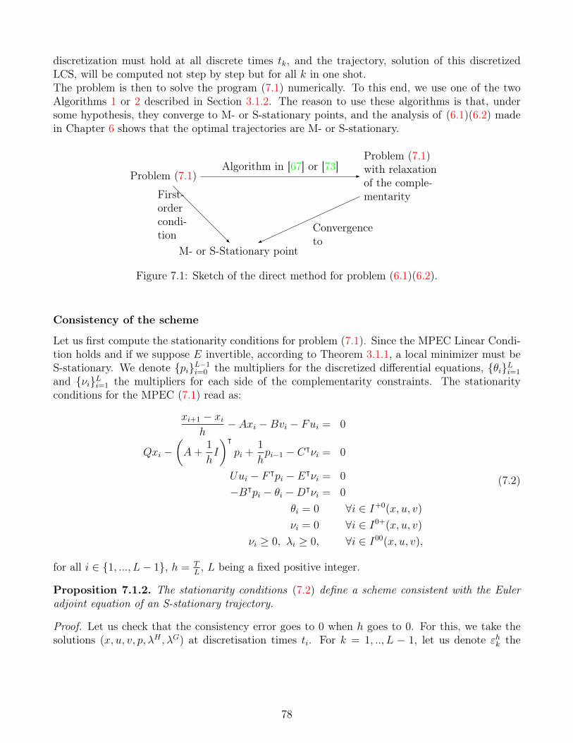
discretization must hold at all discrete times tk, and the trajectory, solution of this discretizedLCS, will be computed not step by step but for all k in one shot.The problem is then to solve the program (7.1) numerically. To this end, we use one of the twoAlgorithms 1 or 2 described in Section 3.1.2. The reason to use these algorithms is that, undersome hypothesis, they converge to M- or S-stationary points, and the analysis of (6.1)(6.2) madein Chapter 6 shows that the optimal trajectories are M- or S-stationary.
Problem (7.1)
Problem (7.1)with relaxationof the comple-mentarity
Algorithm in [67] or [73]
M- or S-Stationary point
First-ordercondi-tion
Convergenceto
Figure 7.1: Sketch of the direct method for problem (6.1)(6.2).
Consistency of the scheme
Let us first compute the stationarity conditions for problem (7.1). Since the MPEC Linear Condi-tion holds and if we suppose E invertible, according to Theorem 3.1.1, a local minimizer must beS-stationary. We denote piL−1
i=0 the multipliers for the discretized differential equations, θiLi=1
and νiLi=1 the multipliers for each side of the complementarity constraints. The stationarityconditions for the MPEC (7.1) read as:
xi+1 − xih
− Axi −Bvi − Fui = 0
Qxi −(A+
1
hI
)ᵀpi +
1
hpi−1 − Cᵀνi = 0
Uui − F ᵀpi − Eᵀνi = 0
−Bᵀpi − θi −Dᵀνi = 0
θi = 0 ∀i ∈ I+0(x, u, v)
νi = 0 ∀i ∈ I0+(x, u, v)
νi ≥ 0, λi ≥ 0, ∀i ∈ I00(x, u, v),
(7.2)
for all i ∈ 1, ..., L− 1, h = TL, L being a fixed positive integer.
Proposition 7.1.2. The stationarity conditions (7.2) define a scheme consistent with the Euleradjoint equation of an S-stationary trajectory.
Proof. Let us check that the consistency error goes to 0 when h goes to 0. For this, we take thesolutions (x, u, v, p, λH , λG) at discretisation times ti. For k = 1, .., L − 1, let us denote εhk the
78
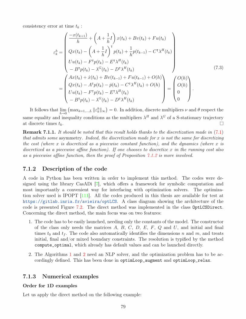
consistency error at time tk :
εhk =
−x(tk+1)
h+
(A+
1
hI
)x(tk) +Bv(tk) + Fu(tk)
Qx(tk)−(A+
1
hI
)ᵀp(tk) +
1
hp(tk−1)− CᵀλH(tk)
Uu(tk)− F ᵀp(tk)− EᵀλH(tk)
−Bᵀp(tk)− λG(tk)−DᵀλH(tk)
=
Ax(tk) + x(tk) +Bv(tk−1) + Fu(tk−1) +O(h)
Qx(tk)− Aᵀp(tk)− p(tk)− CᵀλH(tk) +O(h)
Uu(tk)− F ᵀp(tk)− EᵀλH(tk)
−Bᵀp(tk)− λG(tk)−DᵀλH(tk)
=
O(h)
O(h)
0
0
.
(7.3)
It follows that limh→0
(maxk=1,...,L ‖εhk‖∞
)= 0. In addition, discrete multipliers ν and θ respect the
same equality and inequality conditions as the multipliers λH and λG of a S-stationary trajectoryat discrete times tk.
Remark 7.1.1. It should be noted that this result holds thanks to the discretization made in (7.1)that admits some asymmetry. Indeed, the discretization made for x is not the same for discretizingthe cost (where x is discretized as a piecewise constant function), and the dynamics (where x isdiscretized as a piecewise affine function). If one chooses to discretize x in the running cost alsoas a piecewise affine function, then the proof of Proposition 7.1.2 is more involved.
7.1.2 Description of the code
A code in Python has been written in order to implement this method. The codes were de-signed using the library CasADi [7], which offers a framework for symbolic computation andmost importantly a convenient way for interfacing with optimization solvers. The optimiza-tion solver used is IPOPT [111]. All the codes produced in this thesis are available for test athttps://gitlab.inria.fr/avieira/optLCS. A class diagram showing the architecture of thecode is presented Figure 7.2. The direct method was implemented in the class OptLCSDirect.Concerning the direct method, the main focus was on two features:
1. The code has to be easily launched, needing only the constants of the model. The constructorof the class only needs the matrices A, B, C, D, E, F , Q and U , and initial and finaltimes t0 and tf . The code also automatically identifies the dimensions n and m, and treatsinitial, final and/or mixed boundary constraints. The resolution is typified by the methodcompute_optimal, which already has default values and can be launched directly.
2. The Algorithms 1 and 2 need an NLP solver, and the optimization problem has to be ac-cordingly defined. This has been done in optimLoop_augment and optimLoop_relax.
7.1.3 Numerical examples
Order for 1D examples
Let us apply the direct method on the following example:
79
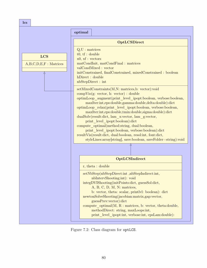
lcs
optimal
OptLCSDirect
Q,U : matricest0, tf : doublex0, xf : vectorsmatCondInit, matCondFinal : matricesvalCondMixed : vectorinitConstrained, finalConstrained, mixedConstrained : booleanhDirect : doublenbStepDirect : int
setMixedConstraints(M,N: matrices,b: vector):voidcompVio(g: vector, h: vector) : doubleoptimLoop_augment(print_level_ipopt:boolean, verbose:boolean,
maxIter:int,eps:double,gamma:double,delta:double):dictoptimLoop_relax(print_level_ipopt:boolean, verbose:boolean,
maxIter:int,eps:double,tmin:double,sigma:double):dictdualSolv(result:dict, lam_x:vector, lam_g:vector,
print_level_ipopt:boolean):dictcompute_optimal(method:string, dual:boolean,
print_level_ipopt:boolean, verbose:boolean):dictresultVis(result:dict, dual:boolean, resol:int, font:dict,
styleLines:array[string], save:boolean, saveFolder=string):void
OptLCSIndirect
r, theta : double
setNbStep(nbStepDirect:int ,nbStepIndirect:int,nbIntervShooting:int): void
integDVIShooting(initPoints:dict, guessSol:dict,A, B, C, D, M, N: matrices,b: vector, theta: scalar, printlvl: boolean): dict
newtonSolveShooting(jacobian:matrix,gap:vector,guessPrev:vector):dict
compute_optimal(M, R : matrices, b: vector, theta:double,methodDirect: string, maxLoops:int,print_level_ipopt:int, verbose:int, epsLam:double):
LCS
A,B,C,D,E,F : Matrices
Figure 7.2: Class diagram for optLCS.
80
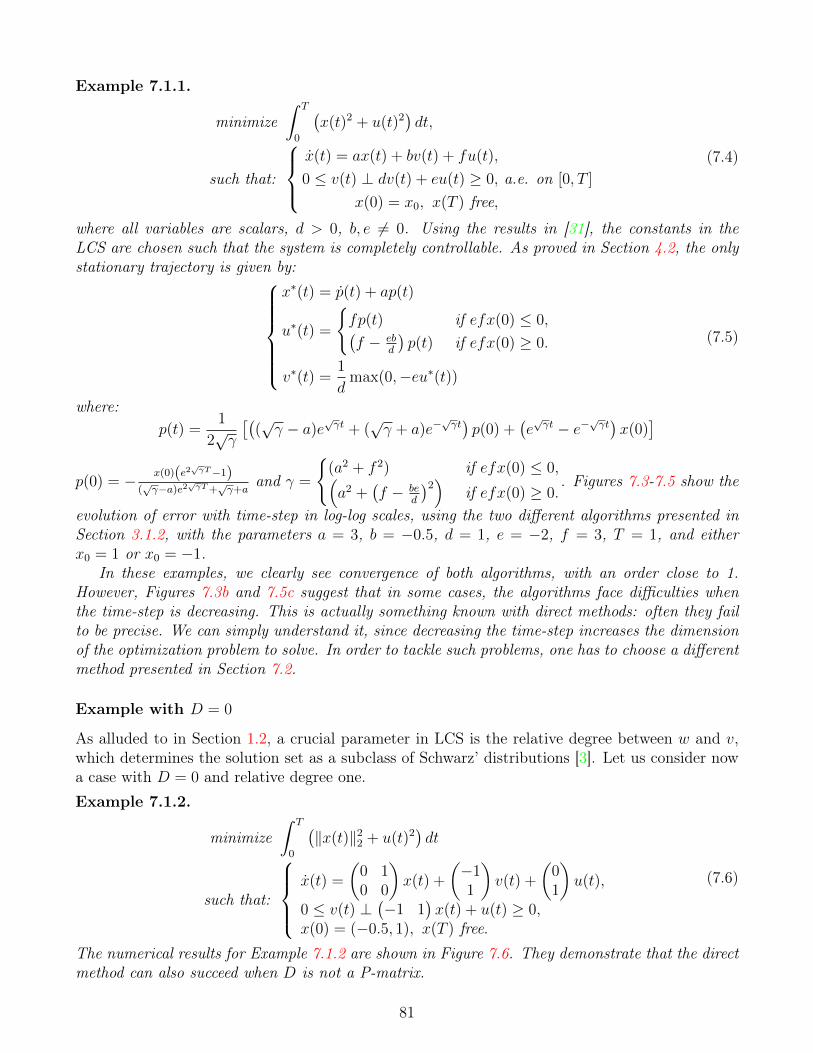
Example 7.1.1.
minimize∫ T
0
(x(t)2 + u(t)2
)dt,
such that:
x(t) = ax(t) + bv(t) + fu(t),
0 ≤ v(t) ⊥ dv(t) + eu(t) ≥ 0, a.e. on [0, T ]
x(0) = x0, x(T ) free,
(7.4)
where all variables are scalars, d > 0, b, e 6= 0. Using the results in [31], the constants in theLCS are chosen such that the system is completely controllable. As proved in Section 4.2, the onlystationary trajectory is given by:
x∗(t) = p(t) + ap(t)
u∗(t) =
fp(t) if efx(0) ≤ 0,(f − eb
d
)p(t) if efx(0) ≥ 0.
v∗(t) =1
dmax(0,−eu∗(t))
(7.5)
where:p(t) =
1
2√γ
[((√γ − a)e
√γt + (
√γ + a)e−
√γt)p(0) +
(e√γt − e−
√γt)x(0)
]p(0) = − x(0)(e2
√γT−1)
(√γ−a)e2
√γT+√γ+a
and γ =
(a2 + f 2) if efx(0) ≤ 0,(a2 +
(f − be
d
)2)
if efx(0) ≥ 0.. Figures 7.3-7.5 show the
evolution of error with time-step in log-log scales, using the two different algorithms presented inSection 3.1.2, with the parameters a = 3, b = −0.5, d = 1, e = −2, f = 3, T = 1, and eitherx0 = 1 or x0 = −1.
In these examples, we clearly see convergence of both algorithms, with an order close to 1.However, Figures 7.3b and 7.5c suggest that in some cases, the algorithms face difficulties whenthe time-step is decreasing. This is actually something known with direct methods: often they failto be precise. We can simply understand it, since decreasing the time-step increases the dimensionof the optimization problem to solve. In order to tackle such problems, one has to choose a differentmethod presented in Section 7.2.
Example with D = 0
As alluded to in Section 1.2, a crucial parameter in LCS is the relative degree between w and v,which determines the solution set as a subclass of Schwarz’ distributions [3]. Let us consider nowa case with D = 0 and relative degree one.Example 7.1.2.
minimize∫ T
0
(‖x(t)‖2
2 + u(t)2)dt
such that:
x(t) =
(0 10 0
)x(t) +
(−11
)v(t) +
(01
)u(t),
0 ≤ v(t) ⊥(−1 1
)x(t) + u(t) ≥ 0,
x(0) = (−0.5, 1), x(T ) free.
(7.6)
The numerical results for Example 7.1.2 are shown in Figure 7.6. They demonstrate that the directmethod can also succeed when D is not a P-matrix.
81

10-4 10-3 10-2 10-1
Time step h
10-5
10-4
10-3
10-2
10-1
Error on state x
Ch a, a=0. 97
(a) Algorithm in [67], x0 = −1
10-4 10-3 10-2 10-1
Time step h
10-4
10-3
10-2
10-1
Error on state x
Ch a, a=0. 68
(b) Algorithm in [73], x0 = −1
10-4 10-3 10-2 10-1
Time step h
10-5
10-4
10-3
10-2
10-1
Error on state x
Ch a, a=1. 02
(c) Algorithm in [67], x0 = 1
10-4 10-3 10-2 10-1
Time step h
10-5
10-4
10-3
10-2
10-1
Error on state x
Ch a, a=1. 01
(d) Algorithm in [73], x0 = 1
Figure 7.3: Error on state x when using Algorithms in [67] or in [73] with a = 3, b = −0.5, d = 1,e = −2, f = 3, T = 1 and x0 = −1 or x0 = 1 in Example 7.1.1.
Higher dimensional examples
For higher dimension or when C 6= 0, we do not have an analytical solution to compare with thenumerical one, but still we can check if the multipliers comply with an S-stationary trajectory. Forthis purpose, let us test them on a third example:
Example 7.1.3.
minimize∫ 1
0
(‖x(t)‖2
2 + 25‖u(t)‖22
)dt,
such that:
x(t) =
(1 22 1
)x(t) +
(−1 1−1 1
)v(t) +
(1 32 1
)u(t),
0 ≤ v(t) ⊥(
3 −1−2 0
)x(t) + v(t) +
(1 −1−1 2
)u(t) ≥ 0, a.e. on [0, 1]
x(0) =
(−1
2
1
), x(T ) free,
(7.7)
where x, u and v are functions [0, 1]→ R2. As shown in Figure 7.7, the Algorithm in [73] seemsto fail to respect the complementarity condition between v2 and w2 at the beginning. The Algorithmin [67] seems to behave better. Comparing first Figure 7.8b and Figure 7.7a, then Figure 7.8c and
82
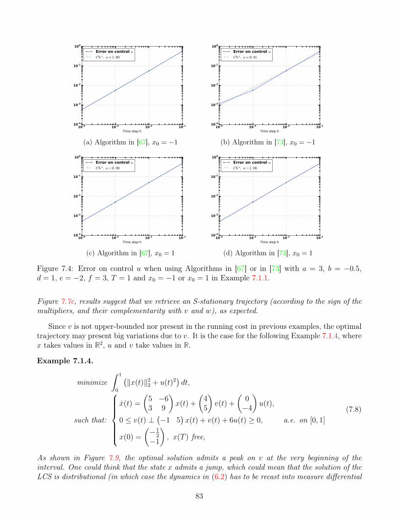
10-4 10-3 10-2 10-1
Time step h
10-4
10-3
10-2
10-1
100
Error on control u
Ch a, a=1. 00
(a) Algorithm in [67], x0 = −1
10-4 10-3 10-2 10-1
Time step h
10-4
10-3
10-2
10-1
100
Error on control u
Ch a, a=0. 91
(b) Algorithm in [73], x0 = −1
10-4 10-3 10-2 10-1
Time step h
10-4
10-3
10-2
10-1
100
Error on control u
Ch a, a=0. 99
(c) Algorithm in [67], x0 = 1
10-4 10-3 10-2 10-1
Time step h
10-4
10-3
10-2
10-1
100
Error on control u
Ch a, a=1. 00
(d) Algorithm in [73], x0 = 1
Figure 7.4: Error on control u when using Algorithms in [67] or in [73] with a = 3, b = −0.5,d = 1, e = −2, f = 3, T = 1 and x0 = −1 or x0 = 1 in Example 7.1.1.
Figure 7.7c, results suggest that we retrieve an S-stationary trajectory (according to the sign of themultipliers, and their complementarity with v and w), as expected.
Since v is not upper-bounded nor present in the running cost in previous examples, the optimaltrajectory may present big variations due to v. It is the case for the following Example 7.1.4, wherex takes values in R2, u and v take values in R.
Example 7.1.4.
minimize∫ 1
0
(‖x(t)‖2
2 + u(t)2)dt,
such that:
x(t) =
(5 −63 9
)x(t) +
(45
)v(t) +
(0−4
)u(t),
0 ≤ v(t) ⊥(−1 5
)x(t) + v(t) + 6u(t) ≥ 0, a.e. on [0, 1]
x(0) =
(−1
2
−1
), x(T ) free,
(7.8)
As shown in Figure 7.9, the optimal solution admits a peak on v at the very beginning of theinterval. One could think that the state x admits a jump, which could mean that the solution of theLCS is distributional (in which case the dynamics in (6.2) has to be recast into measure differential
83
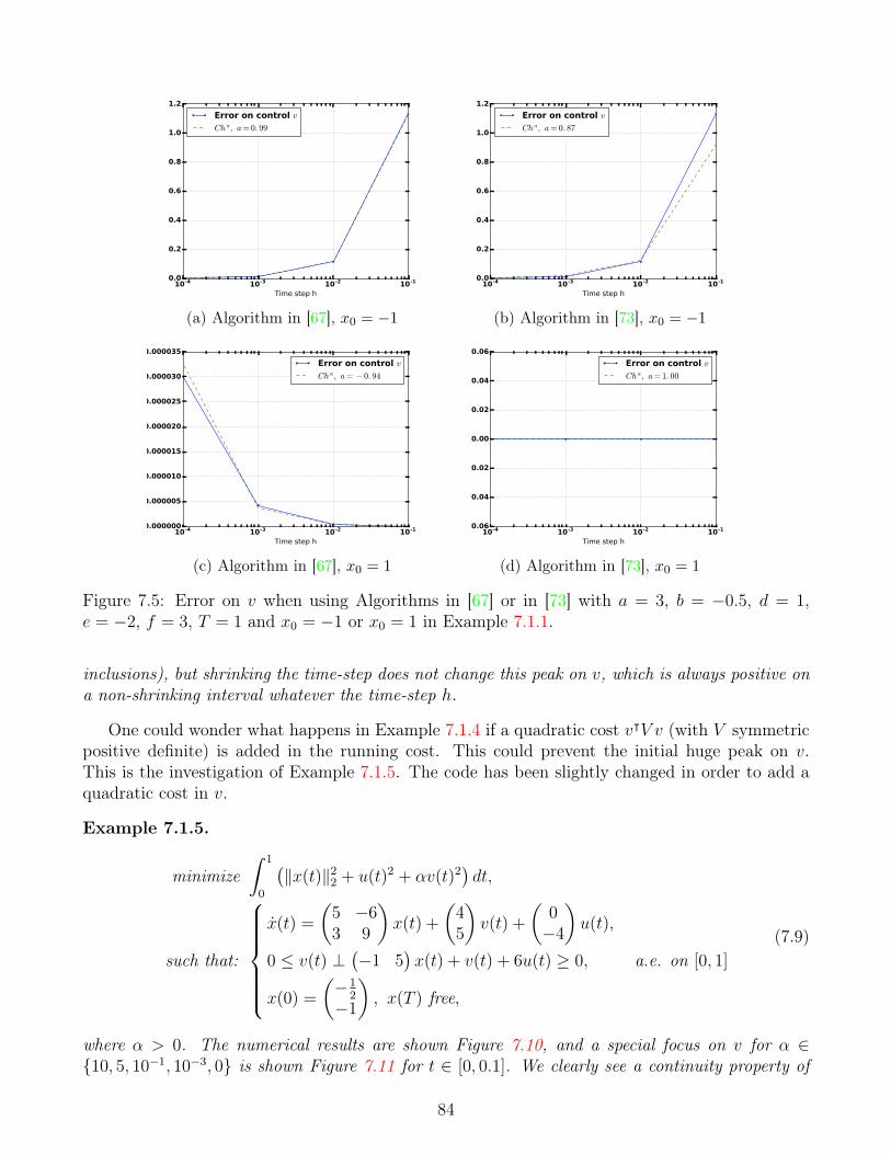
10-4 10-3 10-2 10-1
Time step h
0.0
0.2
0.4
0.6
0.8
1.0
1.2
Error on control v
Ch a, a=0. 99
(a) Algorithm in [67], x0 = −1
10-4 10-3 10-2 10-1
Time step h
0.0
0.2
0.4
0.6
0.8
1.0
1.2
Error on control v
Ch a, a=0. 87
(b) Algorithm in [73], x0 = −1
10-4 10-3 10-2 10-1
Time step h
0.000000
0.000005
0.000010
0.000015
0.000020
0.000025
0.000030
0.000035
Error on control v
Ch a, a= − 0. 94
(c) Algorithm in [67], x0 = 1
10-4 10-3 10-2 10-1
Time step h
−0.06
−0.04
−0.02
0.00
0.02
0.04
0.06
Error on control v
Ch a, a=1. 00
(d) Algorithm in [73], x0 = 1
Figure 7.5: Error on v when using Algorithms in [67] or in [73] with a = 3, b = −0.5, d = 1,e = −2, f = 3, T = 1 and x0 = −1 or x0 = 1 in Example 7.1.1.
inclusions), but shrinking the time-step does not change this peak on v, which is always positive ona non-shrinking interval whatever the time-step h.
One could wonder what happens in Example 7.1.4 if a quadratic cost vᵀV v (with V symmetricpositive definite) is added in the running cost. This could prevent the initial huge peak on v.This is the investigation of Example 7.1.5. The code has been slightly changed in order to add aquadratic cost in v.
Example 7.1.5.
minimize∫ 1
0
(‖x(t)‖2
2 + u(t)2 + αv(t)2)dt,
such that:
x(t) =
(5 −63 9
)x(t) +
(45
)v(t) +
(0−4
)u(t),
0 ≤ v(t) ⊥(−1 5
)x(t) + v(t) + 6u(t) ≥ 0, a.e. on [0, 1]
x(0) =
(−1
2
−1
), x(T ) free,
(7.9)
where α > 0. The numerical results are shown Figure 7.10, and a special focus on v for α ∈10, 5, 10−1, 10−3, 0 is shown Figure 7.11 for t ∈ [0, 0.1]. We clearly see a continuity property of
84
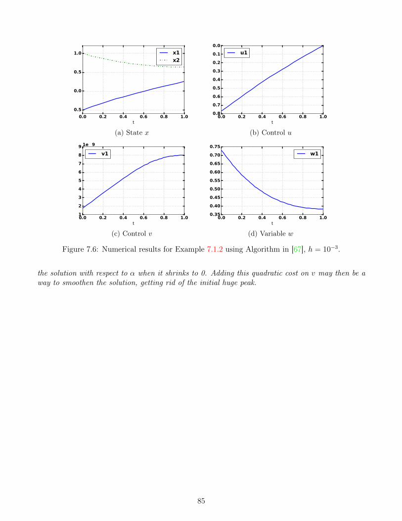
0.0 0.2 0.4 0.6 0.8 1.0t
−0.5
0.0
0.5
1.0 x1
x2
(a) State x
0.0 0.2 0.4 0.6 0.8 1.0t
−0.8
−0.7
−0.6
−0.5
−0.4
−0.3
−0.2
−0.1
0.0
u1
(b) Control u
0.0 0.2 0.4 0.6 0.8 1.0t
1
2
3
4
5
6
7
8
9 1e−9
v1
(c) Control v
0.0 0.2 0.4 0.6 0.8 1.0t
0.35
0.40
0.45
0.50
0.55
0.60
0.65
0.70
0.75
w1
(d) Variable w
Figure 7.6: Numerical results for Example 7.1.2 using Algorithm in [67], h = 10−3.
the solution with respect to α when it shrinks to 0. Adding this quadratic cost on v may then be away to smoothen the solution, getting rid of the initial huge peak.
85
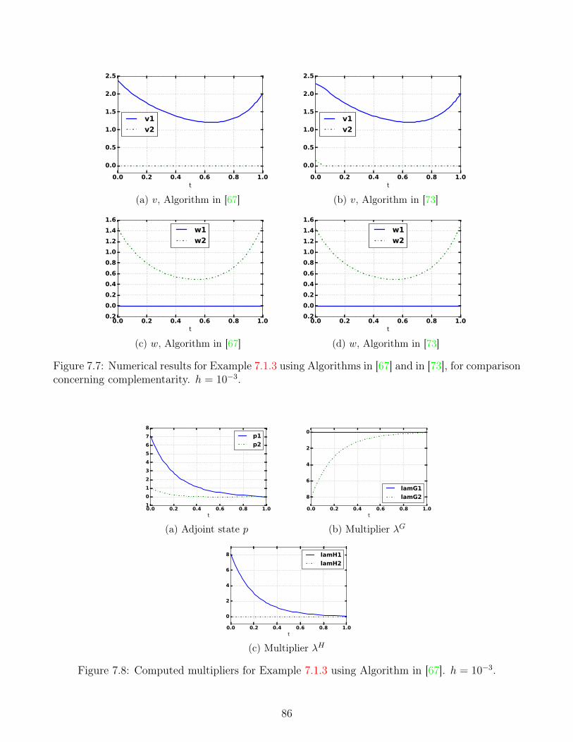
0.0 0.2 0.4 0.6 0.8 1.0t
0.0
0.5
1.0
1.5
2.0
2.5
v1
v2
(a) v, Algorithm in [67]
0.0 0.2 0.4 0.6 0.8 1.0t
0.0
0.5
1.0
1.5
2.0
2.5
v1
v2
(b) v, Algorithm in [73]
0.0 0.2 0.4 0.6 0.8 1.0t
−0.2
0.0
0.2
0.4
0.6
0.8
1.0
1.2
1.4
1.6
w1
w2
(c) w, Algorithm in [67]
0.0 0.2 0.4 0.6 0.8 1.0t
−0.2
0.0
0.2
0.4
0.6
0.8
1.0
1.2
1.4
1.6
w1
w2
(d) w, Algorithm in [73]
Figure 7.7: Numerical results for Example 7.1.3 using Algorithms in [67] and in [73], for comparisonconcerning complementarity. h = 10−3.
0.0 0.2 0.4 0.6 0.8 1.0t
−1
0
1
2
3
4
5
6
7
8
p1
p2
(a) Adjoint state p
0.0 0.2 0.4 0.6 0.8 1.0t
−8
−6
−4
−2
0
lamG1
lamG2
(b) Multiplier λG
0.0 0.2 0.4 0.6 0.8 1.0t
0
2
4
6
8 lamH1
lamH2
(c) Multiplier λH
Figure 7.8: Computed multipliers for Example 7.1.3 using Algorithm in [67]. h = 10−3.
86
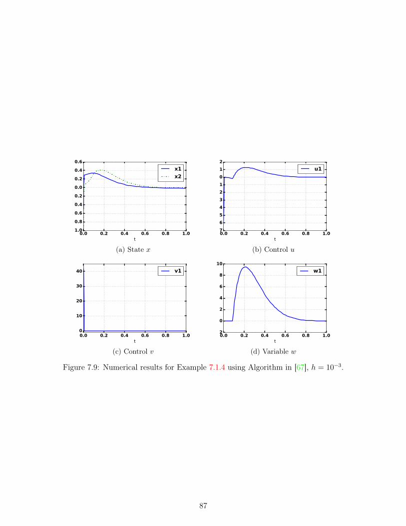
0.0 0.2 0.4 0.6 0.8 1.0t
−1.0
−0.8
−0.6
−0.4
−0.2
0.0
0.2
0.4
0.6
x1
x2
(a) State x
0.0 0.2 0.4 0.6 0.8 1.0t
−7
−6
−5
−4
−3
−2
−1
0
1
2
u1
(b) Control u
0.0 0.2 0.4 0.6 0.8 1.0t
0
10
20
30
40 v1
(c) Control v
0.0 0.2 0.4 0.6 0.8 1.0t
−2
0
2
4
6
8
10
w1
(d) Variable w
Figure 7.9: Numerical results for Example 7.1.4 using Algorithm in [67], h = 10−3.
87

0.0 0.2 0.4 0.6 0.8 1.0t
−1.0
−0.8
−0.6
−0.4
−0.2
0.0
0.2
0.4
0.6
0.8
x1
x2
0.0 0.2 0.4 0.6 0.8 1.0t
0
2
4
6
8
10
12
v1
(a) α = 1
0.0 0.2 0.4 0.6 0.8 1.0t
−1.0
−0.5
0.0
0.5
1.0
1.5
x1
x2
0.0 0.2 0.4 0.6 0.8 1.0t
0
1
2
3
4
5
6
7
v1
(b) α = 10
Figure 7.10: Numerical x and v found for Example 7.1.5 using Algorithm in [67], h = 10−3, anddifferent values of α.
0.00 0.02 0.04 0.06 0.08 0.10t
0
10
20
30
40
v(t)
α=10
α=1
α=1e− 1
α=1e− 2
α=0
Figure 7.11: Numerical v on [0, 0.1] found for Example 7.1.5 using Algorithm in [67], h = 10−3,and different values of α.
88
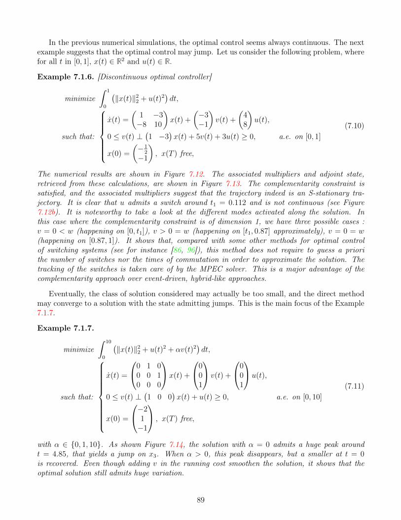
In the previous numerical simulations, the optimal control seems always continuous. The nextexample suggests that the optimal control may jump. Let us consider the following problem, wherefor all t in [0, 1], x(t) ∈ R2 and u(t) ∈ R.
Example 7.1.6. [Discontinuous optimal controller]
minimize∫ 1
0
(‖x(t)‖2
2 + u(t)2)dt,
such that:
x(t) =
(1 −3−8 10
)x(t) +
(−3−1
)v(t) +
(48
)u(t),
0 ≤ v(t) ⊥(1 −3
)x(t) + 5v(t) + 3u(t) ≥ 0, a.e. on [0, 1]
x(0) =
(−1
2
−1
), x(T ) free,
(7.10)
The numerical results are shown in Figure 7.12. The associated multipliers and adjoint state,retrieved from these calculations, are shown in Figure 7.13. The complementarity constraint issatisfied, and the associated multipliers suggest that the trajectory indeed is an S-stationary tra-jectory. It is clear that u admits a switch around t1 = 0.112 and is not continuous (see Figure7.12b). It is noteworthy to take a look at the different modes activated along the solution. Inthis case where the complementarity constraint is of dimension 1, we have three possible cases :v = 0 < w (happening on [0, t1]), v > 0 = w (happening on [t1, 0.87] approximately), v = 0 = w(happening on [0.87, 1]). It shows that, compared with some other methods for optimal controlof switching systems (see for instance [86, 96]), this method does not require to guess a priorithe number of switches nor the times of commutation in order to approximate the solution. Thetracking of the switches is taken care of by the MPEC solver. This is a major advantage of thecomplementarity approach over event-driven, hybrid-like approaches.
Eventually, the class of solution considered may actually be too small, and the direct methodmay converge to a solution with the state admitting jumps. This is the main focus of the Example7.1.7.
Example 7.1.7.
minimize∫ 10
0
(‖x(t)‖2
2 + u(t)2 + αv(t)2)dt,
such that:
x(t) =
0 1 00 0 10 0 0
x(t) +
001
v(t) +
001
u(t),
0 ≤ v(t) ⊥(1 0 0
)x(t) + u(t) ≥ 0, a.e. on [0, 10]
x(0) =
−21−1
, x(T ) free,
(7.11)
with α ∈ 0, 1, 10. As shown Figure 7.14, the solution with α = 0 admits a huge peak aroundt = 4.85, that yields a jump on x3. When α > 0, this peak disappears, but a smaller at t = 0is recovered. Even though adding v in the running cost smoothen the solution, it shows that theoptimal solution still admits huge variation.
89
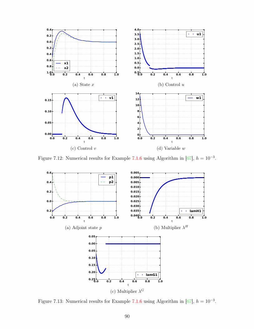
0.0 0.2 0.4 0.6 0.8 1.0t
−1.0
−0.8
−0.6
−0.4
−0.2
0.0
0.2
0.4
x1
x2
(a) State x
0.0 0.2 0.4 0.6 0.8 1.0t
−0.5
0.0
0.5
1.0
1.5
2.0
2.5
3.0
3.5
4.0
u1
(b) Control u
0.0 0.2 0.4 0.6 0.8 1.0t
0.00
0.05
0.10
0.15v1
(c) Control v
0.0 0.2 0.4 0.6 0.8 1.0t
0
2
4
6
8
10
12
14
w1
(d) Variable w
Figure 7.12: Numerical results for Example 7.1.6 using Algorithm in [67], h = 10−3.
0.0 0.2 0.4 0.6 0.8 1.0t
−0.2
0.0
0.2
0.4
0.6
p1
p2
(a) Adjoint state p
0.0 0.2 0.4 0.6 0.8 1.0t
−0.040
−0.035
−0.030
−0.025
−0.020
−0.015
−0.010
−0.005
0.000
0.005
lamH1
(b) Multiplier λH
0.0 0.2 0.4 0.6 0.8 1.0t
−0.25
−0.20
−0.15
−0.10
−0.05
0.00
0.05
lamG1
(c) Multiplier λG
Figure 7.13: Numerical results for Example 7.1.6 using Algorithm in [67], h = 10−3.
90

0 2 4 6 8 10t
−4
−3
−2
−1
0
1
2
3
4
5
x1
x2
x3
0 2 4 6 8 10t
0
200
400
600
800
1000
1200
1400
1600
1800
v1
(a) α = 0
0 2 4 6 8 10t
−3
−2
−1
0
1
2
3
4
5
x1
x2
x3
0 2 4 6 8 10t
0.0
0.2
0.4
0.6
0.8
1.0
1.2
v1
(b) α = 1
0 2 4 6 8 10t
−3
−2
−1
0
1
2
3
4
5
x1
x2
x3
0 2 4 6 8 10t
0.00
0.05
0.10
0.15v1
(c) α = 10
Figure 7.14: Numerical results for x and v for Example 7.1.7 using Algorithm in [67], h = 10−3,using different values for α.
91
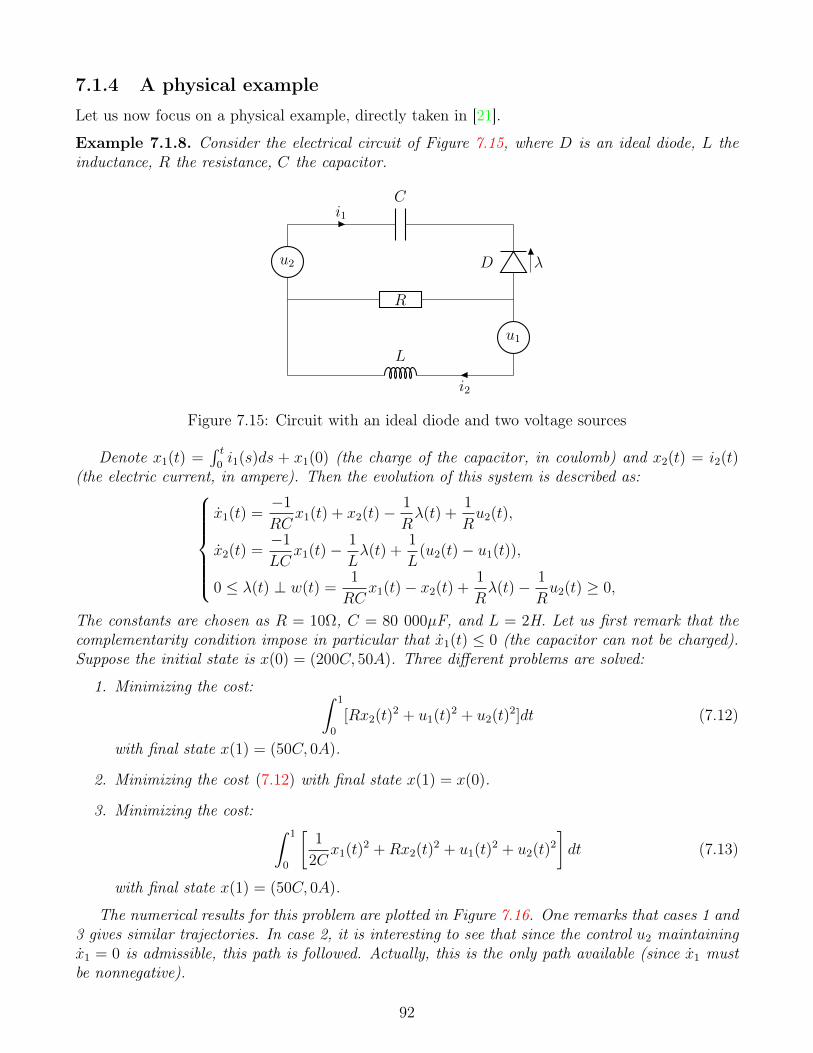
7.1.4 A physical example
Let us now focus on a physical example, directly taken in [21].
Example 7.1.8. Consider the electrical circuit of Figure 7.15, where D is an ideal diode, L theinductance, R the resistance, C the capacitor.
L
i2
D λ
Ci1
R
u1
u2
Figure 7.15: Circuit with an ideal diode and two voltage sources
Denote x1(t) =∫ t
0i1(s)ds + x1(0) (the charge of the capacitor, in coulomb) and x2(t) = i2(t)
(the electric current, in ampere). Then the evolution of this system is described as:x1(t) =
−1
RCx1(t) + x2(t)− 1
Rλ(t) +
1
Ru2(t),
x2(t) =−1
LCx1(t)− 1
Lλ(t) +
1
L(u2(t)− u1(t)),
0 ≤ λ(t) ⊥ w(t) =1
RCx1(t)− x2(t) +
1
Rλ(t)− 1
Ru2(t) ≥ 0,
The constants are chosen as R = 10Ω, C = 80 000µF, and L = 2H. Let us first remark that thecomplementarity condition impose in particular that x1(t) ≤ 0 (the capacitor can not be charged).Suppose the initial state is x(0) = (200C, 50A). Three different problems are solved:
1. Minimizing the cost: ∫ 1
0
[Rx2(t)2 + u1(t)2 + u2(t)2]dt (7.12)
with final state x(1) = (50C, 0A).
2. Minimizing the cost (7.12) with final state x(1) = x(0).
3. Minimizing the cost: ∫ 1
0
[1
2Cx1(t)2 +Rx2(t)2 + u1(t)2 + u2(t)2
]dt (7.13)
with final state x(1) = (50C, 0A).
The numerical results for this problem are plotted in Figure 7.16. One remarks that cases 1 and3 gives similar trajectories. In case 2, it is interesting to see that since the control u2 maintainingx1 = 0 is admissible, this path is followed. Actually, this is the only path available (since x1 mustbe nonnegative).
92
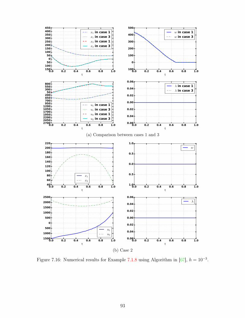
0.0 0.2 0.4 0.6 0.8 1.0t
−150−100−50
050
100150200250300350400450
x1 in case 1
x1 in case 3
x2 in case 1
x2 in case 3
0.0 0.2 0.4 0.6 0.8 1.0t
−100
0
100
200
300
400
500
w in case 1
w in case 3
0.0 0.2 0.4 0.6 0.8 1.0t
−2700−2450−2200−1950−1700−1450−1200−950−700−450−200
50300550800
u1 in case 1
u1 in case 3
u2 in case 1
u2 in case 3
0.0 0.2 0.4 0.6 0.8 1.0t
−0.06
−0.04
−0.02
0.00
0.02
0.04
0.06
λ in case 1
λ in case 3
(a) Comparison between cases 1 and 3
0.0 0.2 0.4 0.6 0.8 1.0t
40
60
80
100
120
140
160
180
200
220
x1
x2
0.0 0.2 0.4 0.6 0.8 1.0t
−1.0
−0.5
0.0
0.5
1.0
w
0.0 0.2 0.4 0.6 0.8 1.0t
−1500
−1000
−500
0
500
1000
1500
2000
2500
u1
u2
0.0 0.2 0.4 0.6 0.8 1.0t
−0.06
−0.04
−0.02
0.00
0.02
0.04
0.06
λ
(b) Case 2
Figure 7.16: Numerical results for Example 7.1.8 using Algorithm in [67], h = 10−3.
93
7.2 Combining direct and indirect methods: the hybrid ap-proach
The indirect method consists in solving the first-order necessary conditions derived in Chapter 6in order to solve the optimal control problem. Since these conditions are necessary and sufficient,solving these equations is equivalent to solving the optimal control problem (6.1)(6.2). As pointedout in [104], it has the advantage that the numerical solutions are usually very precise, but themethod suffers from a huge sensitivity on the initial guess. Indeed, if the initial guess is not closeenough to a solution, then the method may fail to converge.A natural approach is then to use both the direct and the indirect methods in order to obtain avery precise solution, taking advantage of both methods: this is called the hybrid approach. Inour framework, we have to face two problems. First, the active index sets appearing in the Eulerequations (6.4), used to impose conditions on the multipliers, are not useful as they are. Thisproblem has been tackled by re-expressing these equations in Theorem 6.1.2.
7.2.1 Properties of the indirect approach
BVP solver for the indirect method
Solving the first order conditions boils down to solving a Boundary Value Problem (BVP). This isthe case for instance when x(T ) is free; the transversality conditions impose in that case p(T ) = 0.The problem is then to find a solution (x, p) of (6.12) such that x(0) = x0 and p(T ) = 0. Findingsuch a solution is not trivial, especially in this case since the dynamical system is an LCS.
Denote by z =(xp
)and suppose we can rewrite boundary values on z as a linear equation
Mz(0)+ Nz(T ) = xb. Then Theorem 6.1.2 implies that the extremal is a solution of the BoundaryValue Problem (BVP):
(a) z = Az + Bλ(b) 0 ≤ λ ⊥ Dλ+ Cz ≥ 0
(c) Eᵀλ ≥ 0
(d) Mz(0) + Nz(T ) = xb,
(7.14)
where the matrices A, B, C, D and E are easily identifiable from (6.12), and λ =(βv
). This is
a Boundary Value Problem (BVP) formulated for an LCS with constraint (7.14)(c). The shoot-ing method is usually employed to solve such a problem: roughly speaking, given z0 ∈ R2n, wecompute the solution z(·; z0) of (7.14)(a)(b)(c) with initial data z(0) = z0. Letting F (z0) =Mz0 + Nz(T ; z0) − xb, the BVP becomes a root-search of F . In practice, we employ multipleshooting: we also take into account in F shooting nodes inside the interval [0, T ], where we makesure that z(·, z0) is continuous. In the smooth case, we would use a Newton method, which needsthe Jacobian F ′(z0) to compute each iteration leading to the root of F . In our case, the dependenceon z0 of z(T ; z0) is not smooth. Some properties concerning such dependence for LCS have beenderived in [85], as recalled in Section 1.2.5. Broadly speaking, the authors built a linear New-ton Approximation, which allow them to design a non-smooth Newton method for solving BVPfor LCS. However, their result can not be directly applied here for two reasons. First, aside thecomplementarity conditions, we also have to take into account the inequality condition (7.14)(c).Secondly, their result relies on the fact that B SOL(Cz(t),D) is a singleton for all t ∈ [0, T ]. How-ever, this method still could work for (7.14), since the research will only be local. Section 7.2.1
94
shows numerical results where this non-smooth Newton method has been used successfully.
An efficient method to solve the LCS
In the first simulations we ran, we noticed that the integration step by step of the LCS IVP(7.14)(a)(b)(c), z(0) = z0, admitted some numerical instability that multiple shooting could notsolve. This problem was solved using the following proposition:
Proposition 7.2.1. Let ti, ti+1 ∈ [0, T ], ti < ti+1. (z, λ) is a solution ofz = Az + Bλ0 ≤ λ ⊥ Dλ+ Cz ≥ 0
Eᵀλ ≥ 0
z(ti) = zi,
(7.15)
on [ti, ti+1], if and only if it is a global minimum of the optimal control problem:
min
∫ ti+1
ti
λ(t)ᵀ(Dλ(t) + Cz(t))dt
s.t.
z(t) = Az(t) + Bλ(t)
λ(t) ≥ 0
Dλ(t) + Cz(t) ≥ 0
Eλ(t) ≥ 0
a.e. on [ti, ti+1]
z(ti) = zi
(7.16)
with minimum equal to 0.
Proof. ( =⇒ ) Suppose (z, λ) is a solution of (7.15), then (z, λ) is obviously admissible for (7.16),and
∫ ti+1
tiλ(t)ᵀ(Dλ(t) + Cz(t))dt = 0. Suppose there exists an admissible solution (z, λ) of (7.16)
such that∫ ti+1
tiλ(t)ᵀ(Dλ(t) + Cz(t))dt < 0. It then means that there exists τ1, τ2 ∈ [ti, ti+1] such
that [τ1, τ2] is of positive measure and λ(t)ᵀ(Dλ(t) + Cz(t)) < 0 a.e. on [τ1, τ2]. This contradictsthe fact that λ ≥ 0 and Dλ + Cz ≥ 0 a.e. on [ti, ti+1]. Then the minimum is non-negative, and(λ, z) is a global minimum.(⇐=) Suppose (z, λ) is a solution of (7.16). Notice that λ(t)ᵀ(Dλ(t) + Cz(t)) ≥ 0 a.e. on [ti, ti+1],so∫ ti+1
tiλ(t)ᵀ(Dλ(t) +Cz(t))dt = 0 implies that λ(t)ᵀ(Dλ(t) +Cz(t)) = 0 a.e. on [ti, ti+1]. So (z, λ)
is a solution of (7.15).
Numerically, problem (7.16) will be solved for each interval [ti, ti+1] using a classical directmethod, where ti is a node for the Multiple Shooting method. One could ask why this formulationis more stable than just discretizing directly equation (7.15). Intuitively, we can explain it asfollows:
• Using for instance an implicit Euler a discretization of (7.15), one solves at each step theproblem:
zk+1 − zk = h (Azk+1 + Bλk+1)
0 ≤ λk+1 ⊥ Dλk+1 + Czk+1 ≥ 0
Eᵀλk+1 ≥ 0,
95
which takes the form of an LCP with unknown λk+1 and an inequality constraint. But the ex-act solution (z∗k+1, λ
∗k+1) will not be found. Instead, an approximated solution (zk+1, λk+1) =
(z∗k+1 + εk, λ∗k+1 + ελ) will be sought. Then the error will propagate along the solution on
[0, T ], causing instabilities.
• However, if one solves (7.16), all errors will appear under the integral sign. Since this integralis minimized (and we expect the result to be 0), the errors on the whole interval can also beexpected to be minimized.
7.2.2 Description of the code
As for the direct method, a code in Python has been written in order to implement this method.The codes were once again designed using the library CasADi and IPOPT. A class diagram showingthe architecture of the code is presented Figure 7.2. The indirect method was implemented in theclass OptLCSIndirect. Concerning the indirect method, the main focus was on two features:
1. The code has to be as easily launched as the direct method. It only needs, aside what isneeded for the direct method, the matrices M and N appearing in (7.14) and a number ofsteps and shooting nodes for the integration of this equation (via setNbSetp).
2. The multiple shooting has been implemented. There are two aspects to this feature:
• the integration of the dynamics between each shooting node using (7.16). This has beensolved using kind of a direct method with an Euler discretization (since (7.16) is seenas an optimal control problem). This is coded in the method integDVIShooting;
• the non-smooth Newton method, presented in Section 7.2.1. The main focus was onsolving the DI (1.15), and then solving a linear system in order to obtain a descentdirection. It was implemented in newtonSolveShooting.
The shooting algorithm was stopped as soon as the maximum gap at shooting nodes was ofthe order of the time-step (in order to assure continuity of the state and the adjoint state).
7.2.3 Numerical results
Analytical 1D example revisited
First, let us check the convergence of the method of Section 7.2.1 on the 1D Example 7.1.1. Sincethe Direct Method achieved to reach a satisfactory precision, one can expect also the Indirectmethod to converge. The results are presented in Figures 7.17 and 7.18. Overall, the methodreaches the precision of the time step, even for very small precision. Concerning the state x andthe adjoint state p, the convergence is even faster. Concerning λH , λG and v, it seems howeverharder to converge. But still, the desired precision is met, and it is often more precise than theDirect Method.
Example 7.1.3 revisited
In order to compare the Hybrid Approach with the raw direct method, we ran simulations onExample 7.1.3 using different time-steps, and comparing the time spent for solving it at the desiredprecision. The results are shown in Tables 7.1 and 7.2. It appears clearly that, even though the
96

10-5 10-4 10-3 10-2
Time step hI
10-7
10-6
10-5
10-4
10-3
10-2
10-1
Error on state x
Ch a, a=1. 45
(a) Error on x
10-5 10-4 10-3 10-2
Time step hI
10-7
10-6
10-5
10-4
10-3
10-2
Error on adjoint p
Ch a, a=1. 32
(b) Error on p
10-5 10-4 10-3 10-2
Time step hI
10-5
10-4
10-3
10-2
Error on control v
Ch a, a=0. 80
(c) Error on v
10-5 10-4 10-3 10-2
Time step hI
10-6
10-5
10-4
10-3
10-2
Error on multiplier λH
Ch a, a=0. 91
(d) Error on λH
10-5 10-4 10-3 10-2
Time step hI
10-9
10-8
10-7
10-6
10-5
Error on multiplier λG
Ch a, a= − 0. 98
(e) Error on λG
Figure 7.17: Errors with the Hybrid Approach for Example 7.1.1 with a = 3, b = −0.5, d = 1,e = −2, f = 3, T = 1 and x0 = −1.
Indirect method is not that interesting for rough precisions, it becomes necessary for really highprecisions. The Newton Method developed in this context is also satisfying, as shown in Figure7.19, which shows the maximum gap left on x and p at shooting nodes. The program assumesto reach convergence as soon as the continuity on
(xp
)is met with precision h. As shown in this
example, convergence is achieved in two iterations.
Conclusion
In this chapter, two codes for solving numerically the quadratic optimal control of LCS have beendesigned: a direct method, and a hybrid direct/indirect method. These results highlight someproperties of the optimal solution and offer some new perspectives. The methods developed here
97
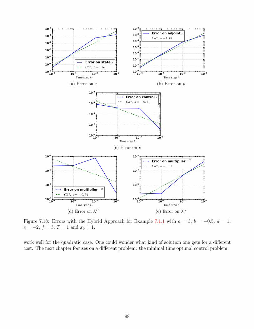
10-5 10-4 10-3 10-2
Time step hI
10-8
10-7
10-6
10-5
10-4
10-3
10-2
Error on state x
Ch a, a=1. 59
(a) Error on x
10-5 10-4 10-3 10-2
Time step hI
10-9
10-8
10-7
10-6
10-5
10-4
10-3
10-2
Error on adjoint p
Ch a, a=1. 78
(b) Error on p
10-5 10-4 10-3 10-2
Time step hI
10-7
10-6
10-5
10-4
10-3
Error on control v
Ch a, a= − 0. 71
(c) Error on v
10-5 10-4 10-3 10-2
Time step hI
10-8
10-7
10-6
10-5
Error on multiplier λH
Ch a, a= − 0. 54
(d) Error on λH
10-5 10-4 10-3 10-2
Time step hI
10-6
10-5
10-4
10-3
Error on multiplier λG
Ch a, a=0. 81
(e) Error on λG
Figure 7.18: Errors with the Hybrid Approach for Example 7.1.1 with a = 3, b = −0.5, d = 1,e = −2, f = 3, T = 1 and x0 = 1.
work well for the quadratic case. One could wonder what kind of solution one gets for a differentcost. The next chapter focuses on a different problem: the minimal time optimal control problem.
98
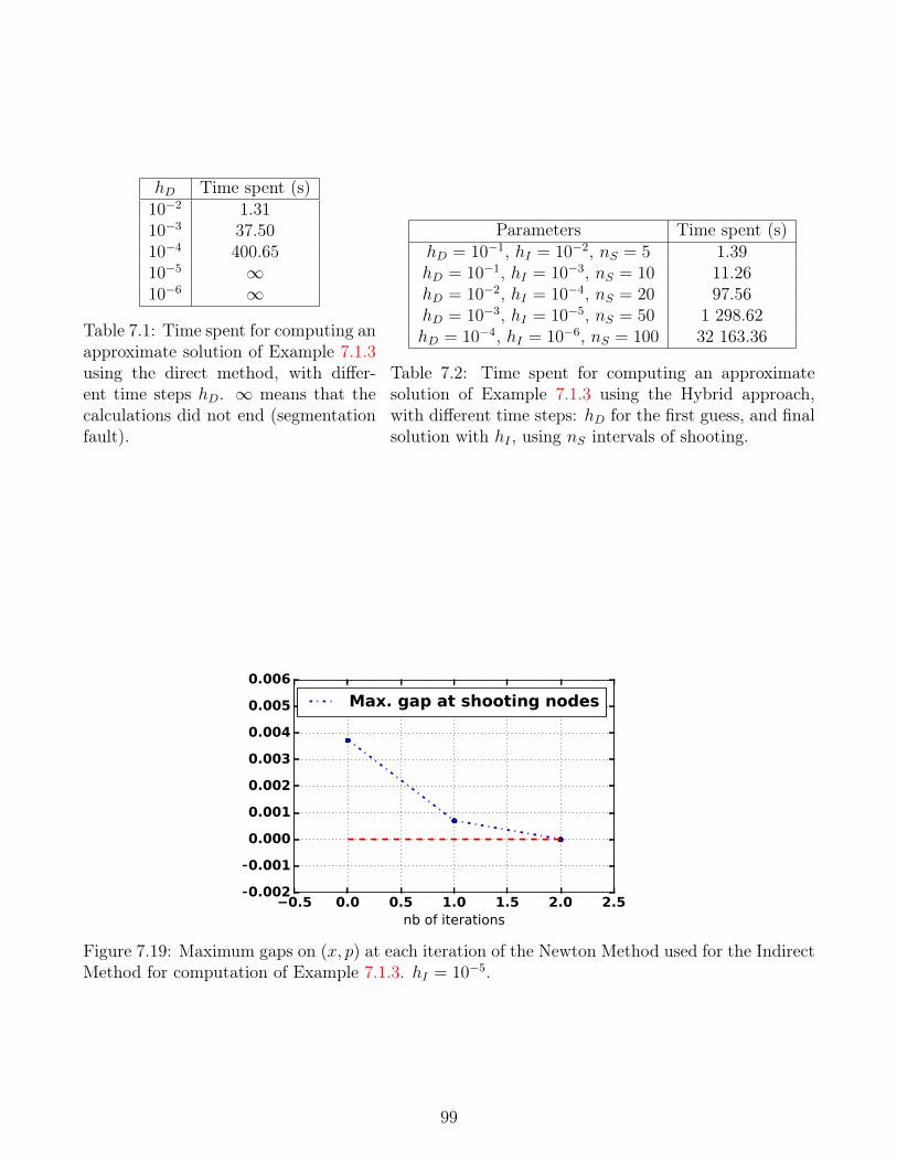
hD Time spent (s)10−2 1.3110−3 37.5010−4 400.6510−5 ∞10−6 ∞
Table 7.1: Time spent for computing anapproximate solution of Example 7.1.3using the direct method, with differ-ent time steps hD. ∞ means that thecalculations did not end (segmentationfault).
Parameters Time spent (s)hD = 10−1, hI = 10−2, nS = 5 1.39hD = 10−1, hI = 10−3, nS = 10 11.26hD = 10−2, hI = 10−4, nS = 20 97.56hD = 10−3, hI = 10−5, nS = 50 1 298.62hD = 10−4, hI = 10−6, nS = 100 32 163.36
Table 7.2: Time spent for computing an approximatesolution of Example 7.1.3 using the Hybrid approach,with different time steps: hD for the first guess, and finalsolution with hI , using nS intervals of shooting.
−0.5 0.0 0.5 1.0 1.5 2.0 2.5nb of iterations
−0.002
−0.001
0.000
0.001
0.002
0.003
0.004
0.005
0.006
Max. gap at shooting nodes
Figure 7.19: Maximum gaps on (x, p) at each iteration of the Newton Method used for the IndirectMethod for computation of Example 7.1.3. hI = 10−5.
99
Part IV
Optimality conditions for the minimal timeproblem
100

Chapter 8
Extension of the nonlinear first orderconditions
Abstract. In this chapter, we extend the results of Section 3.2 in order to tackle the minimaltime problem for systems with complementarity constraints. A special focus is then made on LCS,and we investigate a bang-bang property.
This chapter focuses on finding first order conditions for the minimal time problem:
T ∗ = min T (x, u) (8.1)
s.t.
x(t) = φ(x(t), u(t)),
g(x(t), u(t)) ≤ 0,
h(x(t), u(t)) = 0, a.e. on [0, T (x, u)]
0 ≤ G(x(t), u(t)) ⊥ H(x(t), u(t)) ≥ 0,
u(t) ∈ U(x(0), x(T (x, u))) = (x0, xf ),
(8.2)
with φ : Rn × Rm → Rn, g : Rn × Rm → Rq, h : Rn × Rm → Rp, G,H : [t0, t1] × Rn × Rm → Rl,U ⊂ Rmu , x0, xf ∈ Rn given. We suppose that F and φ are L×B-measurable, where L×B denotesthe σ-algebra of subsets of appropriate spaces generated by product sets M × N , where M is aLebesgue (L) measurable subset in R, and N is a Borel (B) measurable subset in Rn × Rm.We denote a solution of this problem by (T ∗, x∗, u∗). If we don’t bound u with the constraint U ,then the solution will most probably be T ∗ = 0 (i.e. an impulsive control, provided (8.2) is givena mathematical meaning).
The first order conditions given in [59] do not tackle this problem, since therein, the finaltime T ∗ is fixed beforehand. However, slight changes in the proof made for [109, Theorem 8.7.1]allow us to derive first order conditions for (8.1)(8.2). This chapter is organized as follows: first,the necessary conditions for (8.1)(8.2) will be derived. Then, we will show how these results areadapted to the problem of minimal time control for LCS, and some cases where the hypothesis aremet. Finally, the result will be illustrated for a certain class of one dimensional LCS, deriving theanalytical solution.
101
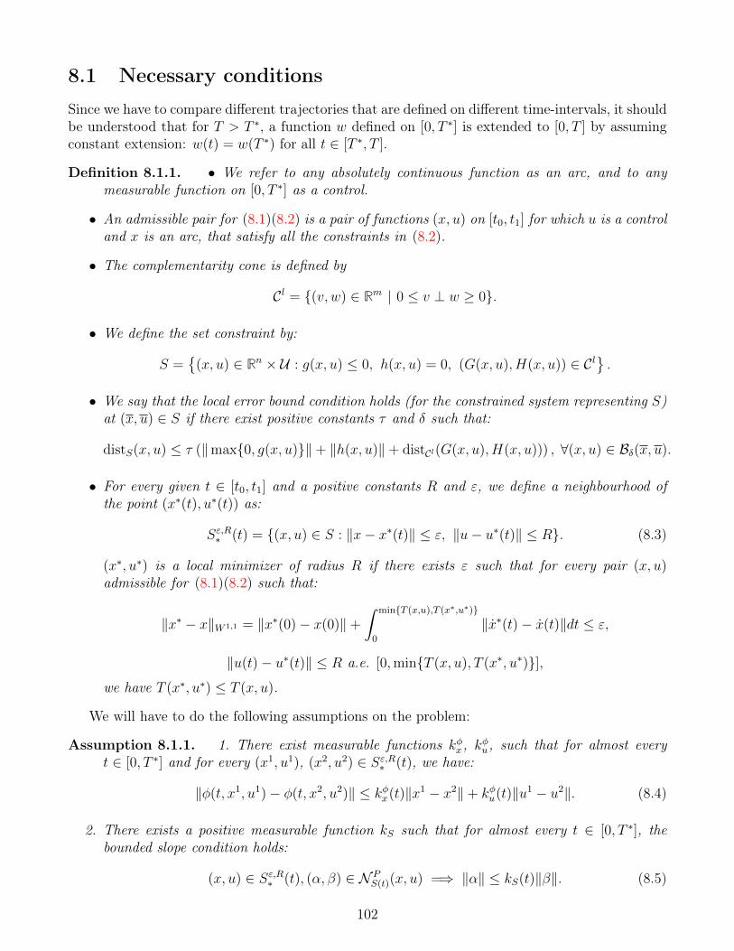
8.1 Necessary conditionsSince we have to compare different trajectories that are defined on different time-intervals, it shouldbe understood that for T > T ∗, a function w defined on [0, T ∗] is extended to [0, T ] by assumingconstant extension: w(t) = w(T ∗) for all t ∈ [T ∗, T ].
Definition 8.1.1. • We refer to any absolutely continuous function as an arc, and to anymeasurable function on [0, T ∗] as a control.
• An admissible pair for (8.1)(8.2) is a pair of functions (x, u) on [t0, t1] for which u is a controland x is an arc, that satisfy all the constraints in (8.2).
• The complementarity cone is defined by
Cl = (v, w) ∈ Rm | 0 ≤ v ⊥ w ≥ 0.
• We define the set constraint by:
S =
(x, u) ∈ Rn × U : g(x, u) ≤ 0, h(x, u) = 0, (G(x, u), H(x, u)) ∈ Cl.
• We say that the local error bound condition holds (for the constrained system representing S)at (x, u) ∈ S if there exist positive constants τ and δ such that:
distS(x, u) ≤ τ (‖max0, g(x, u)‖+ ‖h(x, u)‖+ distCl(G(x, u), H(x, u))) , ∀(x, u) ∈ Bδ(x, u).
• For every given t ∈ [t0, t1] and a positive constants R and ε, we define a neighbourhood ofthe point (x∗(t), u∗(t)) as:
Sε,R∗ (t) = (x, u) ∈ S : ‖x− x∗(t)‖ ≤ ε, ‖u− u∗(t)‖ ≤ R. (8.3)
(x∗, u∗) is a local minimizer of radius R if there exists ε such that for every pair (x, u)admissible for (8.1)(8.2) such that:
‖x∗ − x‖W 1,1 = ‖x∗(0)− x(0)‖+
∫ minT (x,u),T (x∗,u∗)
0
‖x∗(t)− x(t)‖dt ≤ ε,
‖u(t)− u∗(t)‖ ≤ R a.e. [0,minT (x, u), T (x∗, u∗)],
we have T (x∗, u∗) ≤ T (x, u).
We will have to do the following assumptions on the problem:
Assumption 8.1.1. 1. There exist measurable functions kφx , kφu, such that for almost everyt ∈ [0, T ∗] and for every (x1, u1), (x2, u2) ∈ Sε,R∗ (t), we have:
‖φ(t, x1, u1)− φ(t, x2, u2)‖ ≤ kφx(t)‖x1 − x2‖+ kφu(t)‖u1 − u2‖. (8.4)
2. There exists a positive measurable function kS such that for almost every t ∈ [0, T ∗], thebounded slope condition holds:
(x, u) ∈ Sε,R∗ (t), (α, β) ∈ N PS(t)(x, u) =⇒ ‖α‖ ≤ kS(t)‖β‖. (8.5)
102
3. The functions kφx , and kSkφu are integrable, and there exists a positive number η such that
R ≥ ηkS(t) a.e. t ∈ [0, T ∗].
4. φ is L × B-measurable, g, h, G and H are strictly differentiable in variable (x, u).
Let (x∗, u∗) be a local minimizer of (8.1)(8.2). In order to compute the first order conditionof this problem, one introduces a new state variable (as inspired by [109]), absolutely continuous,which will represent time. For any T > 0, denote this variable τ : [0, T ] → [0, T ∗], and let usintroduce x = x τ , u = u τ . Then, for any t ∈ [0, T ]:
˙x(t) = τ(t)x(τ(t)) = τ(t)φ(x(t), u(t)),
0 ≤ G(x(t), u(t)) ⊥ H(x(t), u(t)) ≥ 0.
This method is at the core of the proof for the following Theorem.Define the sets
I−t (x, u) = i ∈ q : gi(x(t), u(t)) < 0,
I+0t (x, u) = i : Gi(x(t), u(t)) > 0 = Hi(x(t), u(t)),
I0+t (x, u) = i : Gi(x(t), u(t)) = 0 < Hi(x(t), u(t)),
I00t (x, u) = i : Gi(x(t), u(t)) = 0 = Hi(x(t), u(t)),
and for any (λg, λh, λG, λH) ∈ Rp+q+2m, denote:
Ψ(x, u;λg, λh, λG, λH) = g(x, u)ᵀλg + h(x, u)ᵀλh −G(x, u)ᵀλG −H(x, u)ᵀλH . (8.6)
Theorem 8.1.1. Suppose Assumption 8.1.1 holds. Let (x∗, u∗) be a local minimizer for (8.1)(8.2).If for almost every t ∈ [0, T ∗] the local error bound condition for the system representing S holdsat (x∗(t), u∗(t)) (see Definition 8.1.1), then (x∗, u∗) is W-stationary; i.e. there exist an arc p :[0, T ∗] → Rn, a scalar λ0 ∈ 0, 1 and multipliers λg : [0, T ∗] → Rq, λh : [0, T ∗] → Rp, λG, λH :[0, T ∗]→ Rm such that:
(λ0, p(t)) 6= 0 ∀t ∈ [0, T ∗], (8.7a)
(p(t), 0) ∈ ∂C 〈−p(t), φ(·, ·)〉 (x∗(t), u∗(t))
+∇x,uΨ(x∗(t), u∗(t);λg(t), λh(t), λG(t), λH(t))
+ 0 × NCU (u∗(t)),
(8.7b)
λg(t) ≥ 0, λgi (t) = 0, ∀i ∈ I−t (x∗, u∗), (8.7c)
λGi (t) = 0, ∀i ∈ I+0t (x∗, u∗), (8.7d)
λHi (t) = 0, ∀i ∈ I0+t (x∗, u∗), (8.7e)
λ0 = 〈p(t), φ(x∗(t), u∗(t))〉. (8.7f)
Moreover, the Weierstrass condition of radius R holds: for almost every t ∈ [0, T ∗] :
(x∗(t), u) ∈ S, ‖u− u∗(t)‖ < R =⇒ 〈p(t), φ(x∗(t), u)〉 ≤ 〈p(t), φ(x∗(t), u∗(t))〉. (8.7g)
103

Proof. Let a ∈ C2([0, T ∗],Rn) be such that a(0) = x∗(0) and ‖a−x∗‖W 1,1 =∫ T ∗
0‖a(t)−x∗(t)‖dt < ε
2.
Let b : [0, T ∗] → Rm be a function such that ‖u∗(t) − b(t)‖ < R2. Let us introduce the following
fixed-end time optimal control problem:
min τ(T ∗) (8.8)
s.t.
˙x(t) = α(t)φ(x(t), u(t)),τ(t) = α(t),z(t) = α(t)‖φ(x(t), u(t))− a(τ(t))‖g(x(t), u(t)) ≤ 0,h(x(t), u(t)) = 0, a.e. on [0, T ∗]0 ≤ G(x(t), u(t)) ⊥ H(x(t), u(t)) ≥ 0,α(t) ∈
[12, 3
2
],
u(t) ∈ U ,‖u(t)− b(τ(t))‖ ≤ R
2,
(x(0), x(T ∗)) = (x0, xf ),τ(0) = 0, |z(0)− z(T ∗)| ≤ ε
2.
(8.9)
Denote by (x, τ, z, u, v, α) an admissible trajectory for (8.8)(8.9), where (x, τ, z) are state variablesand (u, v, α) are controls. We claim that a minimizer for this problem is(
x∗, τ ∗ : t 7→ t, z : t 7→∫ t
0
‖x∗(s)− a(s)‖ds, u∗, v∗, α∗ ≡ 1
)(8.10)
with minimal cost τ ∗(T ∗) = T ∗. To prove this, let us assume that another admissible trajectory(x, τ, z, u, v, α) has a lower cost T = τ(T ∗) < T ∗. Therefore, τ(0) = 0, τ(t) =
∫ t0α(s)ds, and since
α > 0, τ is a continuous strictly increasing function from [0, T ∗] to [0, T ]. Hence it admits aninverse τ−1. Define on [0, T ]:
x = x τ−1, u = u τ−1
and extend these functions to [0, T ∗] by assuming that x(t) = x(T ) for all t ∈ [T, T ∗] (the samegoes for u). Obviously, (x, u) is an admissible trajectory for (8.1)(8.2), with minimal time T . Also,it is in the neighborhood of (x∗, u∗), since for almost all t ∈ [0, T ],
‖u∗(t)− u(t)‖ ≤ ‖u∗(t)− b(t)‖+ ‖u(t)− b(t)‖
≤ R
2+ ‖u(σ)− b(τ(σ))‖ where t = τ(σ)
≤ R
104
and:
‖x− x∗‖W 1,1 =
∫ T
0
‖x(t)− x∗(t)‖dt
≤∫ T
0
‖x(t)− a(t)‖dt+
∫ T
0
‖x∗(t)− a(t)‖dt
≤∫ T
0
‖φ(x(t), u(t))− a(t)‖dt+ε
2
≤∫ T ∗
0
‖φ(x(σ), u(σ))− a(τ(σ))‖τ(σ)dσ +ε
2
≤∫ T ∗
0
‖φ(x(σ), u(σ))− a(τ(σ))‖α(σ)dσ +ε
2
≤ z(T ∗)− z(0) +ε
2≤ ε.
Therefore, since they are in the same neighbourhood, the two trajectories can be compared.Since (x∗, u∗) is supposed to be a local minimizer for (8.1)(8.2), we should have T ∗ ≤ T . This is acontradiction, so the claim that (8.10) is the minimizer was right.Remark that since we supposed that Assumption 8.1.1 is verified, the same assumptions adaptedfor problem (8.8)(8.9) are also valid. Therefore, the results of [59, Theorem 3.2] for (8.8)(8.9) statethat there exists an arc p : [0, T ∗] → Rn, a scalar λ0 ∈ 0, 1 and multipliers λg : [0, T ∗] → Rq,λh : [0, T ∗] → Rp, λG, λH : [0, T ∗] → Rm such that (8.7a)-(8.7e) hold, along with the Weierstrasscondition (8.7g).Notice that since z∗(T ∗) − z∗(0) < ε
2and ‖u∗(t) − b(t)‖ < R
2(the constraints are inactive), these
inequalities do not appear in the first order conditions (the normal cone associated with theseconstraints reduces to 0). Also, one could argue that there should be an adjoint state associatedwith z, but simple calculations show that it is identically 0.Moreover, we should have another arc pτ associated with τ , but it must comply with pτ ≡ 0,pτ (T
∗) = −λ0, such that pτ ≡ −λ0. Also, the stationary inclusion associated with α leads to0 ∈ −〈p, φ(x∗(t), u∗(t))〉− pτ (t) +NC
[ 12 ,32 ]
(α(t)). But since α ≡ 1 and 1 ∈]
12, 3
2
[, NC
[ 12 ,32 ]
(α(t)) = 0for almost every t ∈ [0, T ∗], and so, it yields (8.7f).
8.2 Application to LCS
8.2.1 Sufficient condition for the bounded slope condition
These results still rely on assumptions, among which the bounded slope condition is a stringent,non-intuitive, and hard to verify condition. A sufficient condition for the bounded slope conditionto hold is given by [59, Proposition 3.7], and recalled in Proposition 3.2.1. We give some cases for
105
which this condition holds when the underlying system is an LCS:
T ∗ = min T (x, u, v) (8.11)
s.t.
x(t) = Ax(t) +Bv(t) + Fu(t),
0 ≤ v(t) ⊥ Cx(t) +Dv(t) + Eu(t) ≥ 0, a.e. on [0, T ∗]
u(t) ∈ U(x(0), x(T ∗)) = (x0, xf ),
(8.12)
where A ∈ Rn×n, D ∈ Rm×m, E ∈ Rm×mu , B ∈ Rn×m, F ∈ Rn×mu , C ∈ Rm×n, U ⊆ Rmu . Sinceu is constrained (u(t) ∈ U), in contrast to Chapter 6 for the Linear Quadratic case, the MPECLICQ cannot be used, and therefore we can not prove easily the existence of an S-stationarytrajectory with the same multipliers λG, λH . However, a direct application of [59, Theorem 3.5(b)]to (8.8)(8.9) proves the following proposition.
Proposition 8.2.1. Suppose Assumption 8.1.1 for the problem (8.11)(8.12) holds. Suppose alsothat U is a union of finitely many polyhedral sets. Let (x∗, u∗, v∗) be a local minimizer for (8.11)(8.12).Then, (x∗, u∗, v∗) is M-stationary, meaning it is W-stationary with arc p, and moreover, there existmeasurable functions ηG, ηH : [0, T ∗]→ Rm such that:
0 = Bᵀp+DᵀηH + ηG,
0 ∈ −F ᵀp− EᵀηH +NCU (u∗(t)),
ηGi (t) = 0, ∀i ∈ I+0t (x∗, u∗, v∗),
ηHi (t) = 0, ∀i ∈ I0+t (x∗, u∗, v∗),
ηGi ηHi = 0 or ηGi > 0, ηHi > 0, ∀i ∈ I00
t (x∗, u∗, v∗).
Since the system is linear, [59, Proposition 2.3] asserts that the local error bound conditionholds at every admissible point. There is one case for which one can check that the bounded slopecondition hold: when U = Rmu , as proved in Proposition 6.1.1. However, this case of unboundedU is rather unrealistic, since it could lead to T ∗ = 0 (in the sense that the target xf can bereached from x0 given any positive time T ∗ > 0; see for instance [74] for an example). Whenone attempts to add a constraint U to the previous proof, Proposition 3.2.1 adds a normal conethat prevents checking the inequality, unless one supposes that the optimal trajectory is inside anR-neighbourhood which lies in the interior of U .
Nonetheless, there are two cases when (8.12) verifies the bounded slope condition, even withconstraints on u.
Proposition 8.2.2. Suppose:
• either C = 0,
• or D is a diagonal matrix with positive entries.
Then the bounded slope condition for (8.12) holds.
106
Proof. The case when C = 0 is obvious, when one applies directly Proposition 3.2.1. AssumeD =diag(d1, ..., dm), where the di > 0, i ∈ m, are the diagonal entries of D, and diag means thatD is a diagonal matrix built with these entries. First of all, remark that:
∀λH ∈ Rm, ‖CᵀλH‖ ≤ ‖CᵀD−1‖‖DλH‖.
Now, for t ∈ [0, T ∗] and (x, u) ∈ Sε,R∗ (t), take λG and λH in Rm such that:
λGi = 0, ∀i ∈ I+0t (x, u), λHi = 0, ∀i ∈ I0+
t (x, u),
λGi > 0, λHi > 0, or λGi λHi = 0, ∀i ∈ I00
t (x, u).
It yields:‖DλH‖2 =
∑i∈I+0
t (x,u)
(DiiλHi )2 +
∑i∈I0+t (x,u)
(DiiλHi )2 +
∑i∈I00t (x,u)
(DiiλHi )2
One can easily see that: ∑i∈I+0
t (x,u)
(DiiλHi )2 =
∑i∈I+0
t (x,u)
(DiiλHi + λGi )2,
0 =∑
i∈I0+t (x,u)
(DiiλHi )2 ≤
∑i∈I0+t (x,u)
(DiiλHi + λGi )2,
∀i ∈ I00t (x, u), (Diiλ
Hi )2 ≤ (Diiλ
Hi )2 + (λGi )2 + 2Diiλ
Hi λ
Gi = (Diiλ
Hi + λGi )2.
Therefore, it yields:
‖DλH‖2 ≤m∑i=1
(DiiλHi + λGi )2 = ‖DᵀλH + λG‖2.
One finally proves: ∀ζ ∈ NU(u),
‖CᵀλH‖ ≤ ‖CᵀD−1‖‖DᵀλH + λG‖ ≤ ‖CᵀD−1‖∥∥∥∥DᵀλH + λG
EᵀλH + ζ
∥∥∥∥ .Using Proposition 3.2.1, we see that (8.12) complies with the bounded slope condition.
8.2.2 A bang-bang property
Reachable set for linear systems
We turn ourselves to the reachability set of linear systems in order to state a result that will beuseful in order to prove a bang-bang property for LCS. Consider the following system:
x(t) = Mx(t) +Nu(t),
u(t) ∈ V ,(8.13)
for some matrices M ∈ Rn×n and N ∈ Rn×m. We define the reachable (or accessible) set fromx0 ∈ Rn at time t ≥ 0, with controls taking values in V , denoted by AccV(x0, t), the set of pointsx(t), where x : [0, t] → Rn is a solution of (8.13), with u(s) ∈ V for almost all s ∈ [0, t] andx(0) = x0. As stated in [103, Corollary 2.1.2], which is proved using Aumann’s theorem (see forinstance [39]), the following Proposition shows that the set of constraints V can be embedded inits convex hull:
107
Proposition 8.2.3. [103, Corollary 2.1.2] Suppose that V is compact. Then:
AccV(x0, t) = Accconv(V)(x0, t)
where conv(V) denotes the convex hull of V.
Thanks to Krein-Milman’s Theorem (see Appendix B), this justifies that minimal-time optimalcontrols can be searched as bang-bang controls (meaning, u only takes values that are extremalpoints of V if one supposes in addition that V is convex).
Extremal points for LCS
For this section, let us state the following Assumption:
Assumption 8.2.1. In (8.12), C = 0, D is a P-matrix, and U is a finite union of polyhedralcompact convex sets.
As it can be expected for a minimal time problem with linear dynamics, a bang-bang propertycan be proved, where the bang-bang controls have to be properly defined. Let us define first somenotions. Denote by Ω the constraints on the controls (u, v) in (8.12), meaning:
Ω = (u, v) ∈ U × Rm|0 ≤ v ⊥ Dv + Eu ≥ 0. (8.14)
The set AccΩ(x0, t) denotes the reachable set from x0 ∈ Rn at time t ≥ 0 with controls with valuesin Ω. For a convex set C, a point c ∈ C is called an extreme point if C\c is still convex. This isequivalent to say that:
c1, c2 ∈ C, c =c1 + c2
2=⇒ c = c1 = c2.
The set of extreme points of C will be denoted Ext(C).Suppose Ω is compact (which is not necessarily the case: take for instance D = 0 with 0 ∈ U).
Applying Proposition 8.2.3, one proves that:
AccΩ(x0, t) = Accconv(Ω)(x0, t).
The set Ω is not convex and has empty interior; finding its boundary or extreme points is notpossible in this case. However, Krein-Milman’s Theorem (see Appendix B) proves that conv(Ω)can be generated by its extreme points. In what follows, we will prove that the extreme points ofconv(Ω) are actually points of Ω that can be easily identified from the set U .
For an index set α ⊆ m, denote by Rmα the set of points q in Rm such that qα ≥ 0, qm\α ≤ 0,and define E−1Rmα = u ∈ Rmu|Eu ∈ Rmα (E is not necessarily invertible).
Lemma 8.2.1. Suppose Assumption 8.2.1 holds true. For a certain α ⊆ m, denote by Pα the set:
Pα = (u, v) ∈(U ∩ E−1Rmα
)× Rm|vα = 0, Dα•v + Eα•u = 0, v ≥ 0, Dv + Eu ≥ 0,
and by Eα the set:
Eα = (u, v) ∈ Ext(U ∩ E−1Rmα
)× Rm|vα = 0, Dα•v + Eα•u = 0, v ≥ 0, Dv + Eu ≥ 0.
Then Ext(Pα) = Eα.
108

Proof. If U ∩E−1Rmα is empty, then the equality is obvious. Choose α such that U ∩E−1Rmα is notempty.
• Eα ⊆ Ext(Pα): Let (u, v) ∈ Eα. Suppose that (u, v) 6∈ Ext(Pα). Thus, there exist (u1, v1)and (u2, v2) in Pα, both different than (u, v), such that (u, v) = 1
2[(u1, v1) + (u2, v2)]. But
this implies that u = 12(u1 + u2), and since u ∈ Ext(U ∩ E−1Rmα ), u = u1 = u2. Therefore,
since D is a P-matrix, v = SOL(D,Eu) = SOL(D,Eui) = vi for i ∈ 1, 2. Therefore,(u, v) = (u1, v1) = (u2, v2), and (u, v) is an extremal point of Pα. This is a contradiction.
• Ext(Pα) ⊆ Eα: Let (u, v) ∈ Ext(Pα). Suppose that u 6∈ Ext(U ∩ E−1Rmα ). Therefore, thereexists u1 and u2 in U∩E−1Rmα , different than u, such that u = 1
2(u1+u2). Define for i ∈ 1, 2
vi =SOL(D,Eui). Since Eu1 and Eu2 are members of Rmα , for i ∈ 1, 2:
viα = −(Dαα)−1(Eui)α, viα = 0.
So:vα = −(Dαα)−1(Eu)α =
1
2
(v1α + v2
α
),
vα = 0 =1
2
(v1α + v2
α
).
So (u, v) = 12
[(u1, v1) + (u2, v2)] with (ui, vi) ∈ Pα, i ∈ 1, 2. But since (u, v) ∈ Ext(Pα),u = u1 = u2. This is a contradiction.
Remark 8.2.1. If ker(E) = 0 (and in particular, if E is invertible), it may be easier to searchfor extreme points of the set EU ∩ Rmα , as one can prove easily that:
Ext(U ∩ E−1Rmα ) = E−1Ext(EU ∩ Rmα )
Proposition 8.2.4. Suppose Assumption 8.2.1 holds true. Denote by E the set E =⋃α⊆m Eα,
where Eα is defined in Lemma 8.2.1. Then, for all t > 0 and all x0 ∈ Rn,
AccΩ(x0, t) = AccE(x0, t),
where Ω is defined in (8.14).
Proof. The function SOL(D, ·) : q 7→ v =SOL(D, q) is piecewise linear and continuous, accordingto Proposition 1.1.2. The pieces of SOL(D, ·) are the sets Rmα , for α ranging over the subsets ofm. Therefore, for each α ⊆ m, the set U ∩ E−1Rmα is the union of compact convex polyhedra(possibly empty), and therefore it admits a finite number of extreme points. Thus, each Pα =(u, SOL(D,Eu)) | u ∈ U ∩ E−1Rmα in Lemma 8.2.1 is the union of compact convex polyhedra.In order to simplify the proof, suppose that U (and therefore, each non empty Pα) is a singlecompact convex polyhedron (and not a union of several; the proof would still be the same byreasoning on each of them). Therefore, by Lemma 8.2.1 and Krein-Milman’s theorem (see AppendixB), Pα = conv(Eα) for each subset α of m. Since it can be shown that Ω =
⋃α⊆mPα, it proves:
conv(Ω) = conv
(⋃α⊆m
Pα
).
Let us prove that conv(Ω) =conv(E):
109
• conv(Ω) ⊆conv(⋃
α⊆m Eα): Remark that for all β ⊆ m, Eβ ⊆
⋃α⊆m Eα. Therefore, Pβ =conv(Eβ) ⊆
conv(⋃
α⊆m Eα), and thus, since β was arbitrary, Ω =
⋃α⊆mPα ⊆ conv
(⋃α⊆m Eα
). It then
leads to: conv(Ω) ⊆conv(⋃
α⊆m Eα).
• conv(⋃
α⊆m Eα)⊆conv(Ω):
∀β ⊆ m, Eβ ⊆ conv(Eβ) = Pβ =⇒⋃α⊆m
Eα ⊆⋃α⊆m
Pα = Ω
=⇒ conv
(⋃α⊆m
Eα
)⊆ conv(Ω).
Applying now Proposition 8.2.3, it proves the following equalities:
AccE(x0, t) = Accconv(E)(x0, t) = Accconv(Ω)(x0, t) = AccΩ(x0, t).
The interest of Proposition 8.2.4 is twofold: first, the complementarity constraints does notaffect the bang-bang property that is shared with linear system (it is preserved even for this kindof piecewise linear system); secondly, it is actually sufficient to search for the extreme points ofU ∩ E−1Rmα , as proved in Lemma 8.2.1 with the sets Eα. This result is illustrated in the nextexamples.
Example 8.2.1.
T ∗ = min T (x, u, v) (8.15)
s.t.
x(t) = ax(t) + bv(t) + fu(t),
0 ≤ v(t) ⊥ dv(t) + eu(t) ≥ 0, a.e. on [0, T ∗]
u(t) ∈ U = [−1, 1]
(x(0), x(T ∗)) = (x0, xf ),
(8.16)
where a, b, d, f, e are scalars, and we suppose d > 0 and e 6= 0. We suppose also that there exist atleast one trajectory stirring x0 to xf .
In this case, there are two index sets α as described in Lemma 8.2.1: ∅ or 1. Therefore, weshould have a look at the extreme points of U ∩R1
∅ = U ∩R− = [−1, 0] and of U ∩R11 = U ∩R+ =
[0, 1]. Thus, it is sufficient to look at input functions u with values in −1, 0, 1. Suppose that theconstants in (8.16) (with u(t) supposed unconstrained for the moment) is completely controllable,which means:
If e > 0 : • if f < 0, then b ≥ 0 or [b < 0 and b− fde> 0].
• if f > 0, then b ≤ 0 or [b > 0 and b− fde< 0].
If e < 0 : the same cases as with e > 0 hold by inverting the sign of f .
All other cases (like f = 0 or e = 0) are discarded.Let us now deduce from Theorem 8.1.1 the only stationary solution. First of all, the equation
(8.7b) tells us that the adjoint state complies with the ODE p = −ap. Therefore there exists p0
such that:p(t) = p0e
−at, ∀t ∈ [0, T ∗].
110
Could we have p0 = 0 ? It would imply that p ≡ 0 and then, λ0 = 〈p(t), ax(t) + bv(t) + fu(t)〉 = 0,so (p(t), λ0) = 0 for almost all t in [0, T ∗]. This is not allowed, so p0 6= 0. Moreover, there existmultipliers λG and λH such that, for almost all t in [0, T ∗]:
λG(t) = −bp(t)− dλH(t), (8.17)
λG(t) = 0 if v(t) > 0 = dv(t) + eu(t), (8.18)
λH(t) = 0 if v(t) = 0 < dv(t) + eu(t), (8.19)
fp(t) + eλH(t) ∈ N[−1,1](u(t)) =
0 if |u(t)| 6= 1,
R+ if u(t) = 1,
−R+ if u(t) = −1,
(8.20)
λ0 = max 〈p(t), ax(t) + bv + fu〉,s.t. 0 ≤ v ⊥ dv + eu ≥ 0
(8.21)
(all these equations are derived from (8.7) with g ≡ h ≡ 0, G ≡ v, H ≡ Cx + Dv + Eu,φ ≡ Ax+Bv + Fu). Since d > 0, one can easily prove that:
v =1
dmax(0,−eu).
Let us suppose for now that e > 0 (all subsequent work is easily adapted for e < 0 by replacingu by −u). In this case:
v =
0 if u ∈ [0, 1],
− eud
if u ∈ [−1, 0].(8.22)
Let us now discuss all possible cases for u. If u(t) = 0, then v(t) = 0 = dv(t) + eu(t). We usestationarity conditions for (8.21): since the MPEC Linear Condition holds, there exists multipliersηH and ηG such that ηH = −f
ep(t), ηG =
(dfe− b)p(t), and
ηGηH = 0 or ηH > 0, ηG > 0
(one has M-stationarity, see Definition 3.1.3). However, ηH 6= 0 and ηG 6= 0. Furthermore, ηHhas the same sign as −fp0 and ηG has the same sign as fp0. Therefore, the two have oppositesigns, and u(t) = 0 can not be an M-stationary solution. Therefore, it proves that necessarily, theoptimal control u∗ complies with |u∗(t)| = 1 for almost all t on [0, T ∗].
• If u(t) = 1, then v(t) = 0 < dv(t)+eu(t), and by (8.19), λH(t) = 0. Then by (8.20), fp0 ≥ 0.
• If u(t) = −1, then v(t) > 0 = dv(t) + eu(t), and by (8.17)(8.18), λH(t) = − bdp(t). Then by
(8.20),(f − eb
d
)p0 ≤ 0.
It is impossible to have fp0 ≥ 0 and(f − eb
d
)p0 ≤ 0 at the same time, since f and f − eb
dhave
the same sign by the complete controllability conditions. Therefore, u∗ take only one value along[0, T ∗]: 1 or −1. Then we have two possible optimal state x∗ starting from x0:
if a 6= 0:
x∗(t) =
(x0 + f
a
)exp(at)− f
aif u∗(t) = 1,(
x0 + be−fdad
)exp(at)− be−fd
adif u∗(t) = −1.
111
One must then find the solution that complies with x(T ∗) = xf . One can isolate the optimaltime T ∗:
T ∗ =
1a
ln(axf+f
ax0+f
)if ax0 + f 6= 0 and axf+f
ax0+f> 0,
1a
ln(adxf+be−fdadx0+be−fd
)if adx0 + be− fd 6= 0 and adxf+be−fd
adx0+be−fd > 0.(8.23)
Since we supposed that there exists at least one trajectory stirring x0 to xf , one of these twoexpressions of T ∗ must be positive. Therefore, one can infer that:
u∗ ≡
1 if ax0 + f 6= 0 and axf+f
ax0+f> 0,
−1 if adx0 + be− fd 6= 0 and adxf+be−fdadx0+be−fd > 0.
if a = 0:
x∗(t) =
ft if u∗(t) = 1,be−fddt if u∗(t) = −1.
With the same calculations made in the case a 6= 0, one proves that:
u∗ ≡
1 if f 6= 0 and xf
f> 0,
−1 if be− fd 6= 0 and dxfbe−fd > 0.
The proof of Proposition 8.2.4 relies on the fact that when D is a P-matrix, Ω is the union ofcompact convex polyhedra. However, some examples show that even when D is not a P-matrix,then this property may hold.
Example 8.2.2.
T ∗ = min T (x, u, v) (8.24)
s.t.
x(t) = ax(t) + bv(t) + fu(t),
0 ≤ v(t) ⊥ −v(t) + u(t) ≥ 0, a.e. on [0, T ∗],
u(t) ∈ U = [−1, 1],
(x(0), x(T ∗)) = (x0, xf ).
(8.25)
It is clear that there exists no solution to the LCP(−1, u) appearing in (8.25) for u ∈ [−1, 0), so Ucan actually be restricted to [0, 1]. A graphic showing the shape of Ω and its convex hull is shownin Figure 8.1.
It clearly appears that conv(Ω) is generated by three extreme points:
(u, v) ∈ E = (0, 0), (1, 0), (1, 1).
Exactly the same way as in the proof of Proposition of 8.2.4, one can simply show that for all t ≥ 0and for all x0 ∈ R, AccΩ(x0, t) =AccE(x0, t). Therefore, the optimal trajectory can be searchedwith controls (u, v) with values in E. It is also interesting to note that this bang-bang property canbe guessed from the condition of maximisation of the Hamiltonian in (8.7g) and from Figure 8.1.Indeed, (8.7g) state that at almost all time t, the linear function Λ : (u, v) 7→ 〈p(t), Bv+Fu〉 mustbe maximized with variables (u, v) in Ω. When one tries to maximize Λ over conv(Ω) it becomes aLinear Program (LP) over a simplex. It is well known that linear functions reach their optimumover simplexes at extreme points; in this case, the extreme points are the points of E.
112

u0
v
Ωconv
1
1
Ω
Figure 8.1: Ω and its convex hull for (8.25)
8.2.3 Characterisation through HJB equation
An other way to solve the minimal time optimal control problem is through the Dynamic Program-ming Principle and the Hamilton-Jacobi-Bellman (HJB) equation. The theory needs pure controlconstraints, but not convexity of the set of constraints. Therefore, the Assumption that C = 0 in(8.12) still holds. However, one doesn’t need D to be a P-matrix anymore. The only necessaryAssumption needed is an assumption of compactness.
Assumption 8.2.2. In (8.12), C = 0, and the set Ω defined in (8.14) is a compact subset ofRmu × Rm.
The HJB equation is a non-linear PDE that the objective cost must comply with. In thisframework, the minimal time T ∗ is seen as a function of the target xf . However, the equation willnot be directly met by T ∗(xf ), but by a discounted version of it, called the Kružkov transform,and defined by:
z∗(xf ) =
1− e−T ∗(xf ) if T ∗(xf ) < +∞1 if T ∗(xf ) = +∞
(8.26)
This transformation comes immediately when one tries to solve this optimal control problem withthe running cost:
C(t(xf )) =
∫ t(xf )
0
e−tdt = 1− e−t(xf )
where t(xf ) is a free variable. Minimizing C(t(xf )) amounts to minimizing T ∗. Once one finds theoptimal solution z(xf ), it is easy to recover T ∗, since T ∗(xf ) = − ln(1− z(xf )).
The concept of solution for the HJB equation needs the concept of viscosity solution. Areminder of the definitions of sub- and supersolutions appears in Appendix C. But the most usefuldefinitions are recalled here. First of all, one needs the notion of lower semicontinuous envelope.
113
Definition 8.2.1. Denote z : X → [−∞,+∞], X ⊆ Rn. We call lower semicontinuous envelopeof z the function z˜ defined pointwise by:
z˜(x) = lim infy→x
z(y) = limr→0+
infz(y) : y ∈ X, |y − x| ≤ r
One can see easily that z˜ = z at every point where z is (lower semi-)continuous.Secondly, one needs the definition of an envelope solution.
Definition 8.2.2. Consider the Dirichlet problemF (x, z(x),∇z(x)) = 0 x ∈ κz(x) = g(x) x ∈ ∂κ
(8.27)
with κ ⊆ Rn open, F : κ× R× Rn → R continuous, and g : ∂κ→ R. Denote S = subsolutions of(8.27) and S = supersolutions of (8.27). Let z : κ→ R be locally bounded.
1. z is an envelope viscosity subsolution of (8.27) if there exists S(z) ⊆ S, S(z) 6= ∅, such that:
z(x) = supw∈S(z)
w(x), x ∈ κ
2. z is an envelope viscosity supersolution of (8.27) if there exists S(z) ⊆ S, S(z) 6= ∅, suchthat:
z(x) = infw∈S(z)
w(x), x ∈ κ
3. z is an envelope viscosity solution of (8.27) if it is an envelope viscosity sub- and supersolu-tion.
With these definitions, one can formulate the next Theorem, stating the HJB equation for z∗:
Theorem 8.2.1. z∗ is the envelope viscosity solution of the Dirichlet problem:z +H(x,∇z) = 1 in Rn\xf,z = 0 on xf,
(8.28)
whereH(x, p) = sup
(u,v)∈Ω
〈−p,Ax+Bv + Fu〉.
In case Assumption 8.2.1 is met, then H can be defined as:
H(x, p) = sup(u,v)∈E
〈−p,Ax+Bv + Fu〉, (8.29)
where E has been defined in Proposition 8.2.4.
Proof. By [10, Chapter V.3.2, Theorem 3.7], the lower semicontinuous envelope of z∗, z∗˜ , is theenvelope viscosity solution of the Dirichlet problem (8.28). Thanks to Proposition 8.2.3, one cananalyse the problem equivalently on Ω or on convΩ. Reasoning on convΩ rather than on Ω, onecan prove using [112, Proposition 2.6] that T ∗(·) is a lower semicontinuous function; therefore, sois z∗. It proves that z∗ = z∗˜ and therefore, z∗ is the envelope viscosity solution of (8.28).Finally, Proposition 8.2.4 justifies the expression of H in (8.29).
114
Remark 8.2.2. The target xf could be changed to any closed nonempty set T with compactboundary.
Example 8.2.3. Example 8.2.1 revisited.Let us check that the Kružkov transform of T ∗ found in (8.23) complies with (8.28). The verificationwill be carried in the case when axf+f
ax0+f> 0, the other cases being treated with the same calculations.
In this case, the Kružkov transform of T ∗ defined in (8.26) amounts to:
z∗(xf ) = 1−(ax+ f
ax0 + f
)− 1a
.
Therefore, one must check that
1− z∗(xf ) = −(axf + f
ax0 + f
)− 1a
= sup(u,v)∈Ω
(axf + bv + fu)
dz∗
dx(xf )
(8.30)
where Ω is defined as Ω = (u, v) ∈ −1, 0, 1 × R | 0 ≤ v ⊥ dv + eu ≥ 0.As it has been shown in Example 8.2.1, the sup in (8.30) is attained at u = 1, v = 0. Therefore:
sup(u,v)∈Ω
(axf + bv + fu)
dz∗
dx(xf )
= (axf + f)
(− 1
ax0 + f
(axf + f
ax0 + f
)− 1a−1)
= −(axf + f
ax0 + f
)− 1a
= 1− z∗
Therefore, using the same definition of H made in (8.29), it is proven that z∗ complies with theequation:
z∗ +H
(xf ,
dz∗
dx
)= 1,
which is the HJB Equation (8.28).
Conclusion
The necessary conditions for optimality exposed in Section 3.2 were extended to the case of minimaltime problem. These results were precised for LCS, and some special properties that the optimumpossesses in the case of LCS, were also shown. As future work, one could extend the class of LCScomplying for the Bounded Slope Condition, and also prove the bang-bang property for a broaderclass of LCS, as Example 8.2.2 suggests. Finally, most results presented here do not present statein the constraints: this needs to be enhanced.
115

Conclusion
In this thesis, the optimal control of Linear Complementarity Systems (LCS) has been studied.Two problems were treated: the Linear Quadratic (LQ) optimal control problem with linear com-plementarity, and the minimal time problem for LCS. These two problems show that differentaspects of the study of these systems produce useful results.
For the LQ problem, the main tool we studied are the necessary (and sufficient) conditions ofoptimality. The study of Mathematical Programming with Equilibrium Constraints (MPEC) hintsus that the definition of the multipliers, that are needed for defining properly the stationary condi-tions, are not expressed in a convenient way, neither for analytical purposes nor for computationalones. The main goal in this thesis has been to re-express these conditions in a more numericallytractable way. Eventually, these conditions are expressed as an LCS (with an additional inequal-ity), for which different results are already available. For instance, since these necessary conditionsare often expressed as a Boundary Value Problem (BVP), some results let us construct a way forsolving this problem. This, in turn, leads to the definition of two numerical methods for solvingthe LQ problem, based on the literature. These methods were implemented in a Python code,made in a way such that it is easy to use and to incorporate to a bigger library. The numericalapproximations suggest some properties that the optimal solutions may have, and lead to furtherperspectives.
Concerning the minimal time problem, necessary conditions of optimality were firstly derivedfor a more general, non-linear system with complementarity constraints, that did not appear inthe literature. However, these results, once applied to the case of LCS, seem not as fruitful andinstructive as they are for the LQ case (at least if one want to use them for numerical resolution).A more geometrical approach is then used, in order to prove a bang-bang property for LCS insome cases. This, in turn, can be used in order to simplify the search for an optimal solution.
Perspectives
Of course, as it is customary with any topic of research, this study stimulates other questions.
• Concerning the LQ problem, the set of admissible solutions (the state absolutely continuous,the control in L2) seems definitely too narrow: this is called the Lavrentiev effect. Thenecessary conditions obtained here should be extended to the case of RCBV solutions, assuggested in Section 1.2.3. Some results in [9] may help building these.
• Even in the case of absolutely continuous solutions, the optimality conditions for the LQproblem, written as a BVP where the underlying system is an LCS, is not fully analyzed.For instance, the Theorem 1.2.5 concerning the dependence of the BVP to the initial conditionstill needs to be fully adapted to this problem.
116
• The numerical methods work well for systems of low dimensional complementarity, but itseems harder to make them converge when the dimension is high. A work for enhancing theused algorithms is needed.
• Different assumptions were made across this manuscript, covering different aspects, like theexistence of an optimal solution, or properties that the constraints must meet (like E in-vertible for the LQ problem, D P-matrix for the minimal time problem, or the somewhatrestricting Bounded Slope Condition). Solving these questions or dropping some of theseassumptions, will allow one to apply these results to a bigger range of systems, some of themalready appearing in some engineering problems. A first approach may resemble to the onefound in [13]; it can most certainly be extended to complementarity constraints.
117

Appendix
118
Appendix A
Non-smooth Analysis
Different tools of non-smooth analysis were used in this manuscript. First, let us define the differentnotions of normal cones.
Definition A.0.1. Let Ω ⊆ Rn, and x ∈ cl Ω.
• The proximal normal cone to Ω at x is defined as:
N PΩ (x) = v ∈ Rn : ∃σ > 0; 〈v, y − x〉 ≤ σ‖y − x‖2 ∀y ∈ Ω.
• The limiting normal cone to Ω at x is defined as:
N LΩ (x) = v ∈ Rn : ∃(xk, vk)→ (x, v); vk ∈ N P
Ω (xk) ∀k.
• The Clarke normal cone to Ω at x is defined as NCΩ (x) = cl conv N L
Ω (x).
One can obtain the following inclusions:
N PΩ (x) ⊆ N L
Ω (x) ⊆ NCΩ (x) ∀x ∈ clΩ
Note that when Ω is convex, all these normal cones coincide with the normal cone of convexanalysis (see [91]).
Aside normal cones, one can also define subdifferential of various functions.
Definition A.0.2. Let φ : Rn → R∪+∞ a proper lower semicontinuous function, and x a pointsuch that φ(x) is finite. The limiting subdifferential of φ at x is defined as:
∂Lφ(x) =
v ∈ Rn : ∃(vk, xk)→ (x, v); lim
y→xk
φ(y)− φ(xk)− 〈vk, y − xk〉‖y − xk‖
≥ 0, ∀k
If φ is Lipschitz near x, then the Clarke subdifferential of φ at x can be defined as ∂Cφ(x) = clconv ∂Lφ(x).
119
Appendix B
Krein-Milman Theorem
Since the Krein-Milman Theorem is heavily used in Chapter 8, it is worth recalling its statement.Let us start with a definition.
Definition B.0.1. Let C be a convex compact subset of a Hausdorff locally convex set. Let c ∈ C.The point c is called an extremal point of C if C\c is still convex. Equivalently, c is an extremepoint of C if the following implication holds:
c1, c2 ∈ C, c =1
2(c1 + c2) =⇒ c = c1 = c2
The set of extreme points of C is denoted by Ext(C).
Theorem B.0.1 (Krein-Milman). Let C be a convex compact subset of a Hausdorff locally convexset. Then
C = cl conv (Ext(C))
120
Appendix C
Viscosity solutions
In order to understand some results concerning the HJB equation in Chapter 8, one needs to knowsome definitions related to the concept of viscosity solutions. The definitions given here, extractedfrom [10], are only the ones useful for this manuscript. In particular, the definitions given here arethe ones useful to handle the concept of discontinuous viscosity solutions. The interested readercan find broader results in [10] and the references therein.
Let us first define the notion of subsolution and supersolution of a first order equation
F (x, u,∇u) = 0 in Ω, (C.1)
with Ω ⊆ Rn and F : Ω× R× Rn → R continuous. For this, let us fix some notations: for E ⊆ Rn,denote
USC(E) = u : E → R upper semicontinuous,
LSC(E) = u : E → R lower semicontinuous.
Definition C.0.1. A function u ∈USC(Ω) (resp. LSC(Ω)) is a viscosity subsolution (resp. super-solution) of (C.1) if, for any φ ∈ C 1(Ω) and x ∈ Ω such that u − φ has a local maximum (resp.minimum) at x,
F (x, u(x),∇φ(x)) ≤ 0 (resp. ≥ 0).
121
Bibliography
[1] V. Acary, O. Bonnefon, and B. Brogliato. Time-stepping numerical simulation of switched cir-cuits within the nonsmooth dynamical systems approach. IEEE Transactions on Computer-Aided Design of Integrated Circuits and Systems, 29(7):1042–1055, 2010.
[2] V. Acary, O. Bonnefon, and B. Brogliato. Nonsmooth Modeling and Simulation for SwitchedCircuits, volume 69 of Lecture Notes in Electrical Engineering. Springer Science & BusinessMedia, 2011.
[3] V. Acary, B. Brogliato, and D. Goeleven. Higher order Moreau’s sweeping process: mathem-atical formulation and numerical simulation. Mathematical Programming, 113(1):133–217,2008.
[4] L. Adam and J.V. Outrata. On optimal control of a sweeping process coupled with anordinary differential equation. Discrete & Continuous Dynamical Systems-Series B, 19(9),2014.
[5] S. Adly, T. Haddad, and L. Thibault. Convex sweeping process in the framework of measuredifferential inclusions and evolution variational inequalities. Mathematical Programming,148(1-2):5–47, 2014.
[6] S. Adly, F. Nacry, and L. Thibault. Discontinuous sweeping process with prox-regular sets.ESAIM: Control, Optimisation and Calculus of Variations, 23(4):1293–1329, 2017.
[7] J. Andersson. A General-Purpose Software Framework for Dynamic Optimization. PhDthesis, Arenberg Doctoral School, KU Leuven, Department of Electrical Engineering(ESAT/SCD) and Optimization in Engineering Center, Kasteelpark Arenberg 10, 3001-Heverlee, Belgium, October 2013.
[8] P. Antsaklis and A. Nerode. Hybrid control systems: An introductory discussion to thespecial issue. IEEE Transactions on Automatic Control, 43(4):457–460, 1998.
[9] A.V. Arutyunov, D. Yu Karamzin, and F. L. Pereira. On constrained impulsive controlproblems. Journal of Mathematical sciences, 165(6):654–688, 2010.
[10] M. Bardi and I. Capuzzo-Dolcetta. Optimal control and viscosity solutions of Hamilton-Jacobi-Bellman equations. Springer Science & Business Media, 2008.
[11] S.C. Bengea and R.A. DeCarlo. Optimal control of switching systems. Automatica, 41(1):11–27, 2005.
[12] J. Betts. Practical methods for optimal control and estimation using nonlinear programming,volume 19. Siam, 2010.
122
[13] A. Boccia, M.D.R. De Pinho, and R. Vinter. Optimal control problems with mixed and purestate constraints. SIAM Journal on Control and Optimization, 54(6):3061–3083, 2016.
[14] J. F. Bonnans and A. Hermant. Second-order analysis for optimal control problems withpure state constraints and mixed control-state constraints. In Annales de l’Institut HenriPoincaré (C) Non Linear Analysis, volume 26, pages 561–598. Elsevier, 2009.
[15] B. Bonnard, L. Faubourg, G. Launay, and E. Trélat. Optimal control with state constraintsand the space shuttle re-entry problem. Journal of Dynamical and Control Systems, 9(2):155–199, 2003.
[16] B. Bonnard, L. Faubourg, and E. Trélat. Optimal control of the atmospheric arc of a spaceshuttle and numerical simulations with multiple-shooting method. Mathematical Models andMethods in Applied Sciences, 15(01):109–140, 2005.
[17] M. Branicky, V. Borkar, and S. K. Mitter. A unified framework for hybrid control: Modeland optimal control theory. IEEE Transactions on Automatic Control, 43(1):31–45, 1998.
[18] L.M. Briceno-Arias, N. D. Hoang, and J. Peypouquet. Existence, stability and optimality foroptimal control problems governed by maximal monotone operators. Journal of DifferentialEquations, 260(1):733–757, 2016.
[19] B. Brogliato. Some perspectives on the analysis and control of complementarity systems.IEEE Transactions on Automatic Control, 48(6):918–935, 2003.
[20] B. Brogliato. Absolute stability and the Lagrange–Dirichlet theorem with monotone multi-valued mappings. Systems & Control Letters, 51(5):343–353, 2004.
[21] B Brogliato. Nonsmooth Mechanics. Springer, 2016.
[22] B. Brogliato and L. Thibault. Existence and uniqueness of solutions for non-autonomouscomplementarity dynamical systems. Journal of Convex Analysis, 17(3):961–990, 2010.
[23] M. Brokate and P. Krejčí. Optimal control of ode systems involving a rate independentvariational inequality. Discrete & Continuous Dynamical Systems-Series B, 18(2), 2013.
[24] A.E. Bryson. Applied Optimal Control: Optimization, Estimation and Control. Halsted Pressbook’. Taylor & Francis, 1975.
[25] C. Büskens and H. Maurer. SQP-methods for solving optimal control problems with controland state constraints: adjoint variables, sensitivity analysis and real-time control. Journalof computational and applied mathematics, 120(1-2):85–108, 2000.
[26] K. Camlibel, L. Iannelli, A. Tanwani, and S. Trenn. Differential-algebraic inclusions withmaximal monotone operators. In Decision and Control (CDC), 2016 IEEE 55th Conferenceon, pages 610–615. IEEE, 2016.
[27] M.K. Camlibel, W.P.M.H. Heemels, and J.M.H. Schumacher. Consistency of a time-steppingmethod for a class of piecewise-linear networks. IEEE Transactions on Circuits and SystemsI: Fundamental Theory and Applications, 49(3):349–357, 2002.
123
[28] T. H. Cao and B. S. Mordukhovich. Optimal control of a perturbed sweeping process viadiscrete approximations. Disc. Cont. Dyn. Syst. Ser. B, 21(10):3331–3358, 2015.
[29] C. G Cassandras, D.L. Pepyne, and Y. Wardi. Optimal control of a class of hybrid systems.Automatic Control, IEEE Transactions on, 46(3):398–415, 2001.
[30] C. Castaing and M.D.P. Monteiro Marques. Bv periodic solutions of an evolution problemassociated with continuous moving convex sets. Set-Valued Analysis, 3(4):381–399, 1995.
[31] M.K. Çamlibel. Popov–Belevitch–Hautus type controllability tests for linear complementar-ity systems. Systems & Control Letters, 56(5):381–387, 2007.
[32] M.K. Çamlibel, W.P.M.H. Heemels, and J.M. Schumacher. On linear passive complement-arity systems. European Journal of Control, 8(3):220 – 237, 2002.
[33] M.K. Çamlibel and J.M. Schumacher. On the Zeno behavior of linear complementarity sys-tems. In Decision and Control, 2001. Proceedings of the 40th IEEE Conference on, volume 1,pages 346–351. IEEE, 2001.
[34] L. Cesari. Optimization-Theory and Applications: Problems with Ordinary Differential Equa-tions, volume 17. Springer Science & Business Media, 2012.
[35] M. Chyba, E. Hairer, and G. Vilmart. The role of symplectic integrators in optimal control.Optimal Control Applications and Methods, 30(4):367–382, 2009.
[36] F. Clarke. Optimization and Nonsmooth Analysis, volume 5. SIAM, 1990.
[37] F. Clarke. Necessary Conditions in Dynamic Optimization. Number 816. American Math-ematical Soc., 2005.
[38] F. Clarke and M.D.R. De Pinho. Optimal control problems with mixed constraints. SIAMJournal on Control and Optimization, 48(7):4500–4524, 2010.
[39] F. H. Clarke. A variational proof of Aumann’s theorem. Applied Mathematics and Optimiz-ation, 7(1):373–378, 1981.
[40] F.H. Clarke. The maximum principle under minimal hypotheses. SIAM Journal on Controland Optimization, 14(6):1078–1091, 1976.
[41] G. Colombo and V.V. Goncharov. The sweeping processes without convexity. Set-ValuedAnalysis, 7(4):357–374, 1999.
[42] G. Colombo, R. Henrion, N.D. Hoang, and B.S. Mordukhovich. Discrete approximations ofa controlled sweeping process. Set-Valued and Variational Analysis, 23(1):69–86, 2014.
[43] G. Colombo, R. Henrion, D. H. Nguyen, and B. S. Mordukhovich. Optimal control ofthe sweeping process over polyhedral controlled sets. Journal of Differential Equations,260(4):3397–3447, 2016.
[44] G. Colombo and M. Palladino. The minimum time function for the controlled Moreau’ssweeping process. SIAM Journal on Control and Optimization, 54(4):2036–2062, 2016.
[45] R. Cottle, J.-S. Pang, and R. Stone. The Linear Complementarity Problem. SIAM, 2009.
124
[46] M. d. R. de Pinho. Mixed constrained control problems. Journal of Mathematical Analysisand Applications, 278(2):293–307, 2003.
[47] M.D.R. De Pinho and J. Rosenblueth. Necessary conditions for constrained problems underMangasarian–Fromowitz conditions. SIAM Journal on Control and Optimization, 47(1):535–552, 2008.
[48] M. Diehl, H. G. Bock, H. Diedam, and P-B Wieber. Fast direct multiple shooting algorithmsfor optimal robot control. In Fast motions in Biomechanics and Robotics, pages 65–93.Springer, 2006.
[49] A. V. Dmitruk and A. M. Kaganovich. The hybrid maximum principle is a consequence ofPontryagin maximum principle. Systems & Control Letters, 57(11):964–970, 2008.
[50] A.V. Dmitruk. Maximum principle for the general optimal control problem with phase andregular mixed constraints. Computational Mathematics and Modeling, 4(4):364–377, 1993.
[51] A. Dontchev and W. Hager. The Euler approximation in state constrained optimal control.Mathematics of Computation, 70(233):173–203, 2001.
[52] A. Dontchev, W. Hager, and V. Veliov. Second-order Runge–Kutta approximations in controlconstrained optimal control. SIAM Journal on Numerical Analysis, 38(1):202–226, 2000.
[53] G. Elnagar and M. Kazemi. Pseudospectral Chebyshev optimal control of constrained non-linear dynamical systems. Computational Optimization and Applications, 11(2):195–217,1998.
[54] F. Facchinei and J.-S. Pang. Finite-Dimensional Variational Inequalities and Complement-arity Problems. Springer Science & Business Media, 2007.
[55] A. Giua, C. Seatzu, and C. Van der Mee. Optimal control of switched autonomous linear sys-tems. In Decision and Control, 2001. Proceedings of the 40th IEEE Conference on, volume 3,pages 2472–2477 vol.3, 2001.
[56] D. Goeleven and B. Brogliato. Stability and instability matrices for linear evolution vari-ational inequalities. IEEE Transactions on Automatic Control, 49(4):521–534, 2004.
[57] Q. Gong, M. Ross, W. Kang, and F. Fahroo. Connections between the covector mappingtheorem and convergence of pseudospectral methods for optimal control. ComputationalOptimization and Applications, 41(3):307–335, 2008.
[58] L. Guo, G.-H. Lin, and J. J. Ye. Solving mathematical programs with equilibrium constraints.Journal of Optimization Theory and Applications, 166(1):234–256, 2015.
[59] L. Guo and J. J. Ye. Necessary optimality conditions for optimal control problems withequilibrium constraints. SIAM Journal on Control and Optimization, 54(5):2710–2733, 2016.
[60] W. Hager. Runge–Kutta methods in optimal control and the transformed adjoint system.Numerische Mathematik, 87(2):247–282, 2000.
125

[61] L. Han, A. Tiwari, M.K. Çamlibel, and J.-S. Pang. Convergence of time-stepping schemes forpassive and extended linear complementarity systems. SIAM Journal on Numerical Analysis,47(5):3768–3796, 2009.
[62] M. Hautus and L. Silverman. System structure and singular control. Linear Algebra and itsApplications, 50:369–402, 1983.
[63] W.P.M.H. Heemels, J. M. Schumacher, and S. Weiland. Linear Complementarity Systems.SIAM Journal on Applied Mathematics, 60(4):1234–1269, 2000.
[64] W.P.M.H. Heemels, J.M. Schumacher, and S. Weiland. Well-posedness of linear complement-arity systems. In Decision and Control, 1999. Proceedings of the 38th IEEE Conference on,volume 3, pages 3037–3042. IEEE, 1999.
[65] O. Janin and C.-H. Lamarque. Comparison of several numerical methods for mechanical sys-tems with impacts. International Journal for Numerical Methods in Engineering, 51(9):1101–1132, 2001.
[66] C. Kanzow and A. Schwartz. Mathematical programs with equilibrium constraints: enhancedFritz John-conditions, new constraint qualifications, and improved exact penalty results.SIAM Journal on Optimization, 20(5):2730–2753, 2010.
[67] C. Kanzow and A. Schwartz. A new regularization method for mathematical programswith complementarity constraints with strong convergence properties. SIAM Journal onOptimization, 23(2):770–798, 2013.
[68] M. Kunze and M.D.P. Monteiro Marques. Yosida–Moreau regularization of sweeping pro-cesses with unbounded variation. Journal of Differential Equations, 130(2):292–306, 1996.
[69] Han L., Camlibel M.K., Pang J.-S., and Heemels W.P.M.H. A unified numerical scheme forlinear-quadratic optimal control problems with joint control and state constraints. Optimiz-ation Methods and Software, 27(4-5):761–799, 2012.
[70] J. Lasserre, D. Henrion, C. Prieur, and E. Trélat. Nonlinear optimal control via occupationmeasures and lmi-relaxations. SIAM Journal on Control and Optimization, 47(4):1643–1666,2008.
[71] D. Leenaerts. On linear dynamic complementarity systems. IEEE Transactions on Circuitsand Systems I, 46(8):1022–1026, 1999.
[72] S. Leyffer. MacMPEC: AMPL collection of MPECs, ht-tps://wiki.mcs.anl.gov/leyffer/index.php/macmpec, August 2015.
[73] S. Leyffer, G. López-Calva, and J. Nocedal. Interior methods for mathematical programswith complementarity constraints. SIAM Journal on Optimization, 17(1):52–77, 2006.
[74] J. Lohéac, E. Trélat, and E. Zuazua. Minimal controllability time for finite-dimensionalcontrol systems under state constraints. February 2018. working paper or preprint.
[75] Z.-Q. Luo, J.-S. Pang, and D. Ralph. Mathematical Programs with Equilibrium Constraints.Cambridge University Press, 1996.
126
[76] K. Makowski and L. Neustadt. Optimal control problems with mixed control-phase variableequality and inequality constraints. SIAM Journal on Control, 12(2):184–228, 1974.
[77] B. Maury and J. Venel. A mathematical framework for a crowd motion model. ComptesRendus Mathématique, 346(23-24):1245–1250, 2008.
[78] Michael McAsey, Libin Mou, and Weimin Han. Convergence of the forward-backward sweepmethod in optimal control. Computational Optimization and Applications, 53(1):207–226,2012.
[79] B. Mordukhovich. Variational Analysis and Generalized Differentiation II: Applications,volume 330. Springer Science & Business Media, 2006.
[80] B. Mordukhovich and L. Wang. Optimal control of differential-algebraic inclusions. InOptimal Control, Stabilization and Nonsmooth Analysis, pages 73–83. Springer, 2004.
[81] J.J. Moreau. Evolution problem associated with a moving convex set in a Hilbert space.Journal of Differential Equations, 26(3):347–374, 1977.
[82] J. Outrata. Optimality conditions for a class of mathematical programs with equilibriumconstraints. Mathematics of Operations Research, 24(3):627–644, 1999.
[83] J-S. Pang and M. Fukushima. Complementarity constraint qualifications and simplifiedb-stationarity conditions for mathematical programs with equilibrium constraints. Compu-tational Optimization and Applications, 13(1-3):111–136, 1999.
[84] J.-S. Pang and D. E. Stewart. Differential variational inequalities. Mathematical Program-ming, 113(2):345–424, 2008.
[85] J-S. Pang and D. E. Stewart. Solution dependence on initial conditions in differential vari-ational inequalities. Mathematical Programming, 116(1):429–460, 2009.
[86] B. Passenberg, P.E. Caines, M. Leibold, O. Stursberg, and M. Buss. Optimal control forhybrid systems with partitioned state space. IEEE Transactions on Automatic Control,58(8):2131–2136, 2013.
[87] B. Piccoli. Hybrid systems and optimal control. volume 1, pages 13–18. IEEE, 1998.
[88] L. Pontryagin, V.G. Boltyanskii, R.V. Gamkrelidze, and E.F. Mishchenko. The MathematicalTheory of Optimal Processes. 1962.
[89] R. Pytlak. Numerical Methods for Optimal Control Problems with State Constraints.Springer, 2006.
[90] R. Rockafellar and R.J-B Wets. Variational Analysis, volume 317. Springer Science &Business Media, 2009.
[91] R. T. Rockafellar. Convex Analysis. Princeton university press, 2015.
[92] M. Ross. A roadmap for optimal control: the right way to commute. Annals of the NewYork Academy of Sciences, 1065(1):210–231, 2005.
127
[93] M. Ross and F. Fahroo. Legendre pseudospectral approximations of optimal control prob-lems. In New Trends in Nonlinear Dynamics and Control and their Applications, pages327–342. Springer, 2003.
[94] J.M. Sanz-Serna. Symplectic Runge–Kutta schemes for adjoint equations, automatic differ-entiation, optimal control, and more. SIAM Review, 58(1):3–33, 2016.
[95] H. Scheel and S. Scholtes. Mathematical programs with complementarity constraints: Sta-tionarity, optimality, and sensitivity. Mathematics of Operations Research, 25(1):1–22, 2000.
[96] M.S. Shaikh and P.E. Caines. On the hybrid optimal control problem: theory and algorithms.IEEE Transactions on Automatic Control, 52(9):1587–1603, 2007.
[97] J. Shen and J-S. Pang. Linear complementarity systems: Zeno states. SIAM Journal onControl and Optimization, 44(3):1040–1066, 2005.
[98] G. Smirnov. Introduction to the Theory of Differential Inclusions, volume 41. AmericanMathematical Soc., 2002.
[99] D. Stewart. A high accuracy method for solving odes with discontinuous right-hand side.Numerische Mathematik, 58(1):299–328, 1990.
[100] J. Stoer and R. Bulirsch. Introduction to Numerical Analysis, volume 12. Springer Science& Business Media, 2013.
[101] H. J. Sussmann. A maximum principle for hybrid optimal control problems. In Proceedings ofthe 38th IEEE Conference on Decision and Control (Cat. No.99CH36304), volume 1, pages425–430 vol.1, Dec 1999.
[102] H. J. Sussmann. A nonsmooth hybrid maximum principle. In Stability and Stabilization ofNonlinear Systems, pages 325–354. Springer, 1999.
[103] E. Trélat. Contrôle optimal : Théorie & Applications. Vuibert, 2005. ISBN 2 7117 7175 X.
[104] E. Trélat. Optimal control and applications to aerospace: some results and challenges.Journal of Optimization Theory and Applications, 154(3):713–758, 2012.
[105] R. Vasudevan, H. Gonzalez, R. Bajcsy, and S. Shankar Sastry. Consistent approximationsfor the optimal control of constrained switched systems—part 1: A conceptual algorithm.SIAM Journal on Control and Optimization, 51(6):4463–4483, 2013.
[106] R. Vasudevan, H. Gonzalez, R. Bajcsy, and S. Shankar Sastry. Consistent approximations forthe optimal control of constrained switched systems—part 2: An implementable algorithm.SIAM Journal on Control and Optimization, 51(6):4484–4503, 2013.
[107] A. Vieira, B. Brogliato, and C. Prieur. Preliminary results on the optimal control of linearcomplementarity systems. IFAC-PapersOnLine, 50(1):2977 – 2982, 2017.
[108] A. Vieira, B. Brogliato, and C. Prieur. Quadratic Optimal Control of Linear Complementar-ity Systems: First order necessary conditions and numerical analysis. https://hal.inria.fr/hal-01690400, January 2018.
128
[109] R. Vinter. Optimal Control. Springer Science & Business Media, 2010.
[110] G. Wachsmuth. On LICQ and the uniqueness of Lagrange multipliers. Operations ResearchLetters, 41(1):78–80, 2013.
[111] A. Wächter and L. Biegler. On the implementation of an interior-point filter line-searchalgorithm for large-scale nonlinear programming. Mathematical programming, 106(1):25–57,2006.
[112] P.R. Wolenski and Y. Zhuang. Proximal analysis and the minimal time function. SIAMJournal on Control and Optimization, 36(3):1048–1072, 1998.
[113] J.J. Ye. Optimality conditions for optimization problems with complementarity constraints.SIAM Journal on Optimization, 9(2):374–387, 1999.
[114] J.J. Ye. Necessary and sufficient optimality conditions for mathematical programs withequilibrium constraints. Journal of Mathematical Analysis and Applications, 307(1):350–369, 2005.
[115] J.J. Ye, D.L. Zhu, and Q.J. Zhu. Exact penalization and necessary optimality conditions forgeneralized bilevel programming problems. SIAM Journal on Optimization, 7(2):481–507,1997.
129


