The largest step path following algorithm for monotone linear complementarity problems

Mathematical Programming 76 (1997) 309-332

The largest step path following algorithm for monotone linear complementarity problems

Clovis C. Gonzaga* Department of Mathematics, Federal University of Santa Catarina, Cx. Postal 5210, 88040 Florianopolis,

SC, Brasil

Received 18 May 1994; revised manuscript received 15 May 1996

A b s t r a c t

Path-following algorithms take at each iteration a Newton step for approaching a point on the central path, in such a way that all the iterates remain in a given neighborhood of that path. This paper studies the case in which each iteration uses a pure Newton step with the largest possible reduction in complementarity measure (duality gap).

This algorithm is known to converge superlinearly in objective values. We show that with the addition of a computationally trivial safeguard it achieves Q-quadratic convergence, and show that this behaviour cannot be proved by usual techniques for the original method.

Keywords: Linear complementarity problem; Primal-dual interior-point algorithm; Convergence of algorithms

1. I n t r o d u c t i o n

This paper describes a path-fol lowing algorithm for the monotone horizontal linear

complementar i ty problem, based on following the central path by feasible iterates. The

format of the problem, to be fully described in Section 2, is the following: find (x , s) E R 2n such that

x s = O,

( P ) Qx + R s = b ,

x , s >~ O,

where b E j~n, and Q, R E R n×n are such that for any u, v C ]R n,

i f Qu + Rv = 0 then uTv >10.

* E-mail: [email protected]. Research done while visiting Delft University of Technology, and supported in part by CAPES-Brazil.

0025-5610 Copyright (~) 1997 The Mathematical Programming Society, lnc. Published by Elsevier Science B.V. PH S0025-5610(96)00046-9

310 C.C, Gonzaga/Mathematical Programming 76 (1997) 309-332

This formulation is nice because it includes linear and convex quadratic programming problems expressed by their optimality conditions in their usual format, and also because the related algorithms can be analyzed with very little complexity added to the case of linear programming. Properties of this formulation are described in [2], where it is shown to be equivalent to the usual formulation with a single matrix. This equivalence is also shown in Gtiler [7].

Primal and primal-dual path following methods were developed simultaneously for linear programming. A description of the evolution of these methods until 1990 is found in Gonzaga [4]. Primal-dual methods originated from the description of the central path by Megiddo [ 13], followed by the algorithm of Kojima, Mizuno and Yoshise [ 10]. The same authors [9] and Monteiro and Adler [19,20] developed short step versions of that method which follow the central path in an Euclidean neighborhood and achieve the low complexity bound of O(v/-nL) iterations, where L is the length of the input data. Several variants and extensions of these algorithms for linear programming and linear complementarity problems are extensively described in Kojima, Megiddo, Noma

and Yoshise [8]. Feasible path following algorithms operate essentially as follows: each iteration starts

with a feasible pair (x, s) and a parameter p. > 0 such that the criterion 1 [[xs / t z _ eli <~ or, a c (0,0.5) is satisfied. This is a proximity measure, that certifies ( x , s ) as being near the central point associated with/z. The iteration consists of taking Newton steps (with or without line searches) to approach the condition x s =/z+e, where /z + = T/z, 3/ E (0, 1). The choice of )' in each iteration must be such that all iterates satisfy the proximity condition above. Short steps methods use a fixed value of T near l, and pure Newton steps. The steps can be enlarged by using several Newton steps with line searches in each iteration, but the complexity will fall to O ( n L ) , as shown in Gonzaga

[3]. The proximity measure associated with a feasible pair (x, s) and a parameter/z > 0

used in this paper will be given by the Euclidean norm Ilxs/ - ell. Several other measures are described in [8], but all the algorithms discussed below use the Euclidean norm. Algorithms based on larger neighborhoods have higher complexity, but are usually more efficient in practice. The present technique can be extended to other neighborhoods, but then line searches are needed and the analysis changes.

It is well known that the Newton step is always a combination of the steps for two choices of T: an affine-scaling step, which tries to achieve x s = 0 in one iteration (with T = 0), and the centering step, which tries to reach the central point for /z + = /z (with

T = I ) . Presently the best theoretical results relating convergence rates and computational

complexity are obtained for predictor-corrector algorithms, which alternate affine-scaling steps with line searches and centering steps. The main algorithm was introduced by Mizuno, Todd and Ye [ 17], based on a scheme previously used by Barnes, Chopra and Jensen [ 1 ] for primal linear programming.

I The notation will be discussed ahead in this section.

C.C. Gonzaga/Mathematical Programming 76 (1997) 309-332 311

In the case of linear programming, Ye, Gialer, Tapia and Zhang [26] and independently Mehrotra [ 14] proved Q-quadratic convergence for this algorithm, when considering the predictor and corrector steps as a single iteration. Ye and Anstreicher [25] proved the same rate for linear complementarity problems. The obvious drawback of this scheme is that two linear systems must be solved per iteration, but this can be relieved by the observation that the corrector step computation can reuse the hessian matrix from the predictor: this was proposed by Mehrotra [15], and Gonzaga and Tapia [6] showed that the quadratic rate of convergence is preserved if a safeguard is added to ensure the efficiency of the corrector steps when far from the optimal face.

The need for corrector steps at every iteration can be relaxed, as shown by Ye [24], and this gives rise to algorithms with sub-quadratic rates of convergence. In a very recent paper, Luo and Ye [ 11 ] show how corrector steps can be restrained to a finite number, thus achieving genuine quadratic convergence.

t .1. The largest Newton step

Instead of taking separate predictor and corrector steps, our approach consists in computing the minimum value of ~+ such that the pure feasible Newton step for solving x ' s ~ =/.t+e results in (x+,s +) such that IIx+s+/~ + -e l l ~< ,~. This can be found by computing the affine-scaling and centering directions from (x, s), and by choosing the appropriate combination of these two steps.

This approach was first described in [ 18]. The algorithm in a formulation based on the proximity measure given by the primal-dual potential function was studied by McShane for linear programming and for linear complementarity [ 12]. He proves superlinear convergence under the hypothesis that the iterate sequence converges, and proves quadratic convergence for non-degenerate problems, Bonnans and Gonzaga [2] show that the sequence always converges, thus confirming the superlinear convergence.

In this paper we show the following results: the largest step algorithm becomes quadratically convergent if a simple safeguard is added to the computation of the steplength; without the safeguard, it is not possible to prove quadratic convergence by means of our mathematical tools.

The algorithm and the main result are described in Section 2 and 3. The safeguard is presented in Section 3 for completeness, but its motivation depends on the separate description of the behaviour of the so-called small and large variables, which is done in Sections 4 and 5. Section 6 proves the main results, and ends by describing what can be expected for the original algorithm.

The reason for this behaviour is colloquially described as follows: when centering is used, both large and small variables are centered. If at the beginning of an iteration the large variables are already near their central values, there is much room to play with the small variables (which are responsible for reducing the objective) and /z+/~ = 0(/~) is obtained. Otherwise, this reduction cannot be proved. The safeguard detects the situation in which the large variables are severely off center, and corrects it by increasing the weight of the centering component of the step. The detection of this situation without

312 c.c. Gonzaga/Mathematical Programming 76 (1997) 309-332

the knowledge of the optimal partition is computationally simple, but conceptually not trivial, and will become completely clear only in Section 5.

1.2. Conventions

Given a vector x, d, the corresponding upper case symbol denotes as usual the diagonal matrix X, D defined by the vector. The symbol e will represent the vector of all ones,

with dimension given by the context. Given a matrix A, its null space and column range space are denoted respectively

by .N'(A) and ~ ( A ) . The projection matrix onto .N'(A) is PA, and its complement is

PA =1 --PA. We shall denote component-wise operations on vectors by the usual notations for

real numbers. Thus, given two vectors u, v of the same dimension, uv, u/v, etc. will denote the vectors with components UiUi, Ui/Ui, etc. This notation is consistent as long as component-wise operations always have precedence in relation to matrix operations.

Note that uv - Uv and i rA is a matrix, then Auv - AUv, but in general Auv ~ (Au)v. We shall frequently use the O(. ) and fl (.) notation to express the relationship between

functions. Our most common usage will be associated with a sequence {x k} of vectors and a sequence {/xk} of positive real numbers. In this case x k = O(/zk) means that there

is a constant K (dependent on problem data) such that for every k E N, Ilxktl < K/zk. Similarly, if x k > 0, x k = l~(/zk) means that (xk) - l = O(1/p,k). Finally, x k ~ /zk

means that x k = O(/zk) and x k = fl(/zk).

2. The problem

The monotone linear complementarity problem will be stated in the following format:

find (x, s) E ~2n such that

xs = O, (P) Q x + R s = b ,

x , s >~O,

where b E ~n, and Q, R E R n×n are such that for any u, o E ~n,

if Qu + Rv = 0 then uVv >10.

The feasible set for (P) and the set of interior solutions are respectively

F := { ( x , s ) E R2n I Qx + R s = b , x , s >/ O},

F °:={(x,s) E F [ x > O , s > O } .

We say that x is feasible if there exists s such that (x, s) E F. Similarly, s is feasible

if (x, s) E F for some x.


The set of optimal solutions and the set of strictly complementary optimal solutions

are respectively

~:={(x,s)~Flxs=O}, P:={(x,s)~lx+s>O}.

2.1. Hypotheses

F o ÷ ~ , ~'° + O.

The first hypothesis is necessary for feasible interior point methods. The latter is known as the strict complementarity hypothesis, thoroughly discussed in Monteiro and Wright [22]. It is a common hypothesis in nonlinear programming, without which it is usually impossible to achieve quadratic convergence of algorithms.

2.2. Central points

A feasible solution (x, s) is the central point associated with the parameter/z > 0 if

and only if xs = txe. It is well known (see for instance Kojima, Megiddo, Noma and Yoshise [8] ) that

the set of central points defines a differentiable curve /z > 0 ~ (x(/~), s( /z)) which ends at the analytic center of the optimal face.

Given (x, s) E F and /x > 0, the proximity of (x, s) to (x(/z) , s( /z)) is estimated by the measure

8(x , s , tz) := ~ - e .

We shall assume that an initial interior point (x °, s °) is given, as well as a parameter value/z ° > 0, such that 6(x °, s °,/z °) ~< 0.25.

Given ce E (0, 1 ) and/z °, the Euclidean-norm neighborhood of the central path with

radius a~ is defined as

.M',~ := { (x , s ) E F I ~(x,s , /~) ~< ot for some/z ~< ~o}.

In this paper we shall fix a = 0.25, and all points generated by the algorithms will be

in A/',~. A pair (x, s) is central if and only if it satisfies ~(x, s,/z) = 0 for some/z E (0,/z°].

If 6(x, s,/z) = 6 E (0, 1 ), then

xs - - = e + p , Ilpll = ~- /z

Premultiplying this expression by e T, we obtain

xTs = n/z( l + e), (a)

n

314 C.C. Gonzaga/Mathematical Programming 76 (1997) 309-332

This shows that for points in N',~, /z measures the complementarity error xVs (the duality gap in linear and quadratic programming problems). In particular, at a central point (x, s) = (x( /z) , s(/z) ) , / z = x T s / n .

This justifies path following algorithms, which generate sequences (x k, s k,/Zk) such that/zk ~ 0 and 6 ( x k, s k,/Zk) ~< a E (0, 1 ). The speed of convergence of the algorithms is described in terms of the sequence /Zk: Q-quadratic and Q-superlinear convergence correspond respectively to ~+l/IZk = O(/zk) and/zk+i//zk --* 0.

The path following algorithm will start each iteration from a point (x, s) E .A/',~ and a parameter value/z such that 8(x, s,/~) ~< a, usually coming from the former iteration (see the remarks below). Then it generates a new point ( x + , s +) by computing a Newton iteration for solving the problem below, which corresponds to the search for a point in the central trajectory:

x~ s I = y t ze , Q x I + Rs I = b,

where y E [0, 1 ]. The Newton step for this problem is given by

X + :=Xq--tt, S + :=S-FU,

where u, v are obtained by solving the system

su + xv = - x s + yl~e, Qu + Rv = 0. (2)

It is well known that (see for instance [21]) under our hypotheses the Newton step always has a unique solution (u, v).

We shall frequently deal with the proximity of the resulting point, which justifies the introduction of a special notation for y E (0, 1]:

X+ S+ - - e 6+(',/) := 6( x+, s+, yl~ ) = - ~ . (3)

The computation of 6+(y) is easy from the following argument: x+s + = xs + xv +

su + uv, and from the Newton step, xs + sv + su = ytze. Subtracting these expressions, we deduce that x+s + = uv + y lze and thus for 7' > 0,

6 + ( y ) = u_~ . (4)

Two choices of Y have special interest: ( i ) y = 0: the affine scaling step,

x a = x + u a, s ° = s + v °, (5)

(ii) 9/= 1: the centering step,

x C = x + u c, s c = s + v c. (6)

By superposition, it follows that the Newton step (2) satisfies

(u, v) = "y(u c, v c) "4- ( 1 -- 3/) (u a, va) , (7)

C.C. Gonzaga/ Mathematical Programming 76 (1997) 309-332 315

and the resulting point will be

(x +,s +) =7(x c,s c) + ( 1 - y)(x a,sa). (8)

The path following algorithm will choose at each iteration a value of 7 such that 8+(y) ~< a, so that (x+,s +) E.M~. The largest step in such a scheme will be such that ~ ( y ) = a.

2.3. Remarks on the parameter tz

Most primal-dual path following algorithms associate a parameter with each feasible

pair (x, s) by

x , s e F ° ~ ~ ( x , s) = x+ s / n .

This will not be done in this paper. We start each iteration with (x k, s k,/~k) and take a pure Newton step (2) to generate (x k+l , sk+l,y/Zk). There are several reasons why we

believe this to be the best choice: (i) It simplifies the theory, since the variation o f /z becomes trivially known. (ii) If Qu+Rv = 0 implies uTv = 0 (as in a problem coming from linear programming

or a skew symmetric linear complementarity problem), then both approaches coincide. In fact, given any (x, s,/1.) C F °, consider the Newton step (2), with Y C (0, 1]. We

have

(X + u)T(s q- U) = xT s -~- xTu q- sTl.t -'~ uTo = n"/Id, -]- uTv.

If uTv = 0, then y/z = (x+)Ts+/n. If this is not the case, then it is proved in [2] that uTv = O(/z2), and the approaches tend to coincide for small values of ~.

(iii) In any case, expression ( 1 ) shows that for any choice of /z such that 8(x, s,/z) ~< 0.25, /z(x, s) >/ /1.(1 - 1/4x/n). The improvement that can be obtained by choosing /z(x, s) is worse than 2.5% for n/> 100.

(iv) This is our most important remark. Given (x, s) C F °, the proximity to the central path should be measured by

8*(x,s)=min,~>o ~ - e I "

The unique minimizer is easily computed by differentiation, giving

~*(x, ~,)- Ilxsll2 xTs •

We conclude that the largest pure Newton step is obtained by substituting the following expression for (3) :

x+ s+ e 8+(Y)=~*(x+'s+)= ~*(x+, s+)

The largest step is computed by choosing y such that 8+(y) = 0.25. The computation of the step is more complicated, and we believe that it would not pay because of (iii).


Anyway, all the results derived in this paper can be easily extended to this choice of parameter, simply by observing that all the lemmas are still true if we give an extra reduction in IZk in the beginning of each iteration (keeping 3(x k, s k,/zk) ~< 0.25, of course).

(v) Finally, the largest possible step based on Newton directions is obtained by minimizing /z*(x, s) in the intersection of A/'~ and the bidimensional region defined by adding combinations of the centering and affine-scaling directions to the point of departure. The computational efficiency of this procedure is unknown.

3. The algorithm

In this section we describe the algorithm and list its convergence properties. The remainder of the paper will be dedicated to the proof of these results. From here on, we make the choice a = 0.25. The results can certainly be adapted for any positive

a ~< 0.25. We start by stating the algorithm with no safeguard.

Algorithm 1. Data: e > 0, (x° ,s °) E .N',, P~o E (0,/z °] such that 8(x°, s°,p.0) ~< 0.25.

k : = 0 R E P E A T

X : = X k, S : = S k, /£ : = /L/, k.

Compute (u c, v c) and (u" , v a) by solving the Newton equations (2) for y = l

and y = 0. Find Yk equal to the largest 7 E (0, 1) such that 2

6 + ( ~ ) = ( y u c + (1 -7)ua)(yvC+ ( 1 - y)v") =0.25. (9)

( x k+l , s k+l ) := (x, s) + y(u c, v c) + ( 1 - y) (u% v°).

/zk+l := y/z. k : = k + l .

U N T I L /z k < e .

Remarks. • Developing the expression for o~-(y) in the algorithm, one immediately sees that

it reduces to the solution of a quartic equation in y. We choose the largest root in (0, 1) to avoid complications with multiple crossings of the boundary of A/'~. In fact, the only thing that will be assumed in the theoretical development is that whenever

8+(0.1) >/0.25, Yk >1 0.1. • In this paper we shall assume that the computation is done exactly, but this is by no

means necessary. A sound way of computing y is the following: use a bisection scheme, stopping it at the first iteration in which it finds yl , 72 such that l > yl > 72, yl ~< 23/2,


and 6 + ( y l ) ~< a < 6+(3"2), then choose 3" = 3"I. Due to the technicality above, the

bisection scheme should start with the values O, O. 1, 1 for 3".

3.1. The safeguard

The algorithm in a similar formulation was studied by McShane for linear programming and for linear complementarity [12]. This algorithm converges superlinearly, but

we will show in Section 6 that it does not seem possible to prove quadratic convergence. This can nevertheless be remedied by a safeguard added before the computation of 7 in the algorithm. The safeguard will be described here for completeness, but we are aware that at this point the reader will probably not be able to understand its motivation.

A l g o r i t h m 2. Data: e > 0, (x °, s t ) E A/',~,/~0 E (0 , /z °] such that 8 (x °, s t , /zo) ~< 0.25.

k : = 0 R E P E A T

X : = X k, S : = S k, td,:=/d, k.

Compute (uC, v c) and (ua,v a) by solving the Newton equations (2) for 3" = 1

and 3 /=0 . I f 6+(0 .1 ) E (0 .2 ,0 .25) then choose Y E [0.1,0.7]

Else find 3' such that 8+(3,) = 0.25. (x~+l, s k+l ) := ( x , s ) +y(uC,v ¢) + (1 - 3")(ua,v~).

3'k := 3', /zk+l := 3"/z. k : = k + l .

UNTIL /zk < e

An interesting choice for 3" in the safeguard, which will be justified later, is 3/= 0.7. The safeguard is related to the behaviour of the so called large variables, which will

be described in the next section. The safeguard step is a realization of the following ideal command: let x* be the analytic center of the optimal face;

"I f the large variables are far from x* then enforce some centralization"

We shall show in the next section that the condition 6+(0.1) > 0.2 detects the

situation in which x is far from x*. Once we decide that centering is needed, there are several possible actions. The easiest

one is to take 3" = 1, and do a pure centering step as predictor-corrector algorithms do. We decided to complicate things a bit, and show that limited centering is sufficient. The number 0.1 was chosen arbitrarily: any e ~< 0.1 can be used in the safeguard step. An interesting way of rewriting the algorithm uses the following safeguard:

Find 3' such that 6+(3") = 0.25. I f 3 ' < 0.01 then if 6+(0 .1) > 0.2 then choose 3" E [0.01,0.7] .


The following facts will be proved in the analysis of the next section: (i) In an iteration in which the safeguard is not triggered, "Yk = O(ixk).

If bisection is used to compute 71 as above, then 71 ~< 2"yk = O(Ixk). (ii) There exists an integer J such that: if at an iteration k >~ J the step y = 0.7 is

taken, then the safeguard will never be triggered again in subsequent iterations; for any choice of ~/ E [0.1,0.7], the safeguard can be triggered no more than 7 /7 times after k = J.

These two facts prove the Q-quadratic convergence of Ixk.

3.2. Polynomial convergence

If instead of choosing "y as in the algorithm, one uses a certain small fixed value near 1, then the short steps methods of Kojima, Mizuno and Yoshise [9] and Monteiro and Adler [ 19] are reproduced. Then polynomial complexity of O ( v ~ L ) iterations is obtained. The step chosen by our algorithm is certainly longer than this short step, and one concludes that the complexity is preserved.

Now we present a proof of this fact, for completeness.

Lemma 1. At any iteration of Algorithm 1 or 2, 9' ~< 1 - 0.1/v'-n. The algorithms stop in O( x/-nL ) iterations, where L = ln(ix0/e).

Proof. Let (x, s, IX) be the data at the beginning of an arbitrary iteration. The first assertion in the Lemma is true by construction if the safeguard is used. Otherwise, we shall use the following central result in interior point methods (see for instance [ 16] ): if 6 = ~(x, s, yix) ~< 0.5, then fi(x +, s +, ?IX) < 82, where (x +, s ÷) is the point resulting from a Newton step (2).

All we need to prove is that if 8(x ,s , ix) ~< 0.25 and 1 >/ 7 /> 1 - 0.1/x/-n then 8(x, s,),/.t) ~< 0.5: the result above then guarantees that the algorithms do not choose ~'

in this interval. Let a E [0,0.1/x/n] , 8 = 8(x, s, ( 1 - a) ix) . We have

XS e 8 = (1 --~)IX

and hence

( 1 - o t ) ~ = XS-e+aetx ~<0.25+x/~a~<0.35.

It follows that ~ ~< 0.35/0.9, proving the linear convergence result. After k iterations, the algorithms obtain Ixk ~< (1 --0.1/x/-n)~IX0 and hence

0 , k In ~<kln 1 - 0.I ~ < - - - ~ - .

It follows that k ~< lOv/nln(ix0/ix~), and at termination k ~< lOv, rffL, completing the proof. []

C.C Gonzaga/ Mathematical Programming 76 (1997) 309-332 319

If the bisection scheme is used, this Lemma implies that y ~< 1 - 0.05/v/-n will be

found. The computation of y does not increase the complexity: using the bisection scheme

and counting each step of the bisection algorithm as one full iteration (disregarding

the fact that its internal complexity is very low), the following is true: either y E [0.1,1 - 0 . 05 /v~ ] and then a fixed number of bisection iterations will be sufficient, or each step of bisection divides/z by 2, which is much better than a complete short step. In fact, for k sufficiently large, yk < 0.5 because of the superlinear asymptotic

convergence, and from this point on the total number of bisection iterations is dominated by O(L) . Of course, this does not establish any lower complexity bound.

4. Analysis of the algorithm

Our scope is proving the assertions made in the last section. The analysis depends

on being able to describe separately the behaviour of the so-called small and large variables. This study is made in Bonnans and Gonzaga [2], and here we list the main

results without proofs. The optimal set ~ is a face of the polyhedron F, characterized by a partition {B, N}

of the index set { I . . . . . n}, so that for all (x, s) C .r "r'°, x8 > 0, xN = 0, sB = 0, sN > 0.

The vectors composed by (xB, sN) and (xN, sB) are called respectively the vectors of large and small variables.

Finding this optimal partition is as difficult as solving the original problem, and hence its knowledge cannot be assumed in the algorithms. But when we analyze the behaviour of a given sequence, we can assume that the partition is known. A great simplification is obtained if for the analysis we reorder the variables according to the following scheme:

The constraint Qx + Rs = b is rewritten as

[Q8 Rs] sN xN

And now the variables are renamed in the following sequence:

Q ~ [Q8 RNJ, R ~ [RB QNI, x*-- , s~-- . ( I0 ) SN XN

With this reordering, the optimal face is characterized simply by

f = { (x , s ) ClR2"ls=O, Qx=b,x>~O}. (11)

Monotonicity is not affected by reordering. In addition, the Newton directions are

invariant with respect to this transformation. This means that all algorithms based on the Newton step are invariant with respect to the permutation of variables. Of course the algorithms never use the knowledge of the optimal partition.

From now on, we assume that the variables are ordered as above, and thus x and s are respectively the vectors of large and small variables. We also assume for the remainder


of this section that (x, s) E .N'a and ,u. C (0 , /z ° ] are given, and study the Newton step from this point. The Newton equations remain unchanged,

su + xv = - x s + Ttze, Qu + Rv = 0. (12)

4. I. Scaled equations

Let us define the scaling vector d = V/-~-/s and scale the variables by

Yc=d-lx, ~ = d - l u , g=ds/Iz, ~=dv/tz. (13)

Other scaled variables like ~a, etc. are defined similarly. Note that this scaling differs from the usual one by the presence o f / z in the expressions. This only makes sense

because x and s are now the large and small variables. This scaling transfers the given x and s to the same vector xv/

~b = d - i x = --~- = (14)

and the proximity measure is given by

= 2 - e l ] . (15)

The scaled equations become, after dividing by/x~b,

~ + 0 = -~b + T~b -1 , QDii=-tzRD-~5, (16)

and ~To >~ 0 whenever ~, t7 satisfy the constraint above.

4.2. Solution of the scaled equations

Let us introduce one more simplification in notation, by defining

A=QD.

Following [2] , we know that with the monotonicity condition, any dual 3 feasible

direction ~ satisfies

O E "R.(AT).

Using this fact, one can prove that ~ is the projection of the right-hand side of the first equation in (16) onto the affine subspace defined by A~ = -I~RD-I~. But the

right-hand side of this equation is small, I~RD-I~ = O(/~), and thus (see [2] )

fi = PA(--t~ q- Ttb -1 ) --t- O(/.t.). (17)

Another interesting fact related to the scaled problem is the following: since any optimal solution (x*, s*) satisfies s* = 0, any feasible vector of small variables s is also

3 We shall frequently call x and s respectively 'primal' and "dual' variables. This is an obvious abuse of language, mainly after having reordered the variables.


a feasible direction s - s*. In particular for the scaled problem, ¢ is a dual feasible direction, and thus ¢ E T~(AT), i.e.

PA¢ = 0 , P A ¢ = ¢ , (18)

where/sA = 1 - Pa. The relevant properties of the scaled Newton step are described in the following

lemma.

Lemma 2. The solution (~, 5) of the scaled Newton equations (16) satisfy:

ri = PA(--¢ "1- •¢-1 ) .q~ O(At) = ~PA¢ - l + O(At),

O = PA(--¢ + ~/¢-' ) + O(At) = --¢ 4- TPA, ¢-1 + O(/z),

I~T5 = O(At).

Proof. Let (~, 0) be the solution of the scaled equations (16). Then t]+O = - ¢ + T ¢ -I Substituting (17),

p~(_¢ + ~,¢-1) + ~ = ( _ ¢ + T¢-1) + o (~) .

Since ~ E 7"~(AT), this is the unique orthogonal decomposition of the right-hand side along JV'(A) and T~(AT). It follows that

= PA(--¢ + ~/¢-1 ) + PAt(At) = PA(--¢ + , y ¢ - l ) + O(At).

The other expressions for the projections follow from the fact that PA¢ = 0. By direct substitution, one also deduces that ~To = O(/z), completing the proof. []

4.3. Sizes

For (x, s) E .N'~, it is well known that x ,-~ 1. See for instance Monteiro and Tsuchiya [21]. Using the fact that 8 (x , s , At) ~< a, it follows that s ,-~ At. Using these facts and Lemma 2, the following size limitations can be proved (detailed proofs are found in [2]):

x ~ l , s"~be, d - ,~ l , ¢ , ~ 1 ;

~ = O(T) + O(/x), 0 = O(1) , (19)

u = O ( ~ , ) + O ( A t ) , v = o ( A t ) .

The next lemma uses these sizes to expose very interesting properties of the affine- scaling step.

Lemma 3. Consider the affine-scaling step (u a, v a) from (x, s), obtained from the Newton equations with 7 = O. Then

x ~ = x + O ( A t ) , s ~ = O ( A t 2 ) .

322 C. C. Gonzaga/ Mathematical Programming 76 (1997) 309-332

Proof. From (19) with 7 = 0, u a = 0( /2) and hence x a = x + u a = x + O(/2), proving the first equality. We have:

s a = s + v ° = / 2 d - l (~b + ~a).

From Lemma 2 with y = O, ~ = -~b + 0( /2) , and it follows that s a =/2d- tO( /2) . Since d -I ,,~ l, this completes the proof. []

We are ready for the central result of this paper: a description of the behaviour of 6+ (7) , as 7 varies in (0, 1 ]. Most of our subsequent work will be the analysis of the expression in the lemma below, illustrated by Fig. 1.

Lemma 4. Consider a Newton iteration f r o m an interior pa i r (x, s) E A/'~ a n d / 2 > O,

and the proximi ty y C (0, 1 ] ~ 6 + ( y ) , defined in (3) . Let ( x c, s c) be the result o f the

centering step (6 ) . Then

xsc e 0 ( / 2 ) 6+(y) ~< (1 - y ) - ~ - + y6(xC, sC,/2) + - - ,y

xsC -- e 6+(7) ) ( 1 - - y ) -~- - y6(xC, sC,/2) - 9(/2)y

Proof. The Newton step is given by the superposition (8): for y E (0, 1], using Lemma

3,

x + = y x c + (1 -- y ) x a = y x c + (1 - y ) x + 0( /2) ,

s + = y s c + (I - y ) s ° = y s ~ + 0 ( / 2 2 ) .

Now compute x+s +, noting that x+O(/22) = 0(/22) and scO(/2) = O(/2 z) because s c = 0 ( / 2 ) .

x+s+ = Y 2xcsc + Y( 1 - y ) x s c + 0(/22).

Dividing by 7/2 > 0 and subtracting e = y e + ( 1 - y ) e,

--x+s+Y/2 -e=y(x~i-e)+(1-y)(x~ c e ) + O(/2)-3 /

Taking norm~ and using the triangle inequality, the expressions in the lemma follow, completing the proof. []

Our results will stem from the analysis of the expressions in the lemma above. In these expressions, the term 8 ( x c, s c, /2) is easy: it is the proximity after a centering step, very well known. It is small, and for 8(x, s,/2) <~ 0.25, we shall prove in Lemma 7 that 8 ( x c, s c , /2) <~ 0.03.

The term ot = IlxsC//2 - ell is not so simple. It is related to the primal proximity of x, and we will show that if x is nearly centered according to a primal-only proximity

C.C. Gonzaga/Mathematical Programming 76 (1997) 309-332

6+(9")

323

0 0.1 - - y , 1 8( x ~, s * , tz)

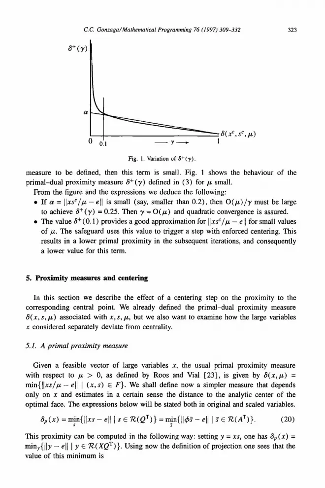
Fig. I. Variation of 6+(y).

measure to be defined, then this term is small. Fig. 1 shows the behaviour of the pr imal-dual proximity measure 8+(9") defined in (3) for p, small.

From the figure and the expressions we deduce the following: • I f a = ]lxsC/I ~ - eli is small (say, smaller than 0.2), then O( /z ) /9 ' must be large

to achieve 8+(9") = 0.25. Then 9' = O(/z) and quadratic convergence is assured. • The value 8 + (0.1) provides a good approximation for IlxsC/ - ell for small values

o f / z . The safeguard uses this value to trigger a step with enforced centering. This results in a lower primal proximity in the subsequent iterations, and consequently a lower value for this term.

5. Proximity measures and centering

In this section we describe the effect of a centering step on the proximity to the corresponding central point. We already defined the primal-dual proximity measure

6(x , s, tz) associated with x, s,/x, but we also want to examine how the large variables x considered separately deviate from centrality.

5.1. A pr imal proximity measure

Given a feasible vector of large variables x, the usual primal proximity measure

with respect to /~ > 0, as defined by Roos and Vial [23] , is given by 6 ( x , tz) =

m in{ l l x s / t z - ell I ( x , s ) E V}. We shall define now a simpler measure that depends only on x and estimates in a certain sense the distance to the analytic center of the optimal face. The expressions below will be stated both in original and scaled variables.

8 p ( X ) =nfi. n{llxs-ell IsE~(QT)}=~n{Ilck~-elIIgE~(AT)}. ( 2 0 )

This proximity can be computed in the following way: setting y = xs, one has 8p(X) =

miny{lly - ell I Y E ~ ( X Q T ) } . Using now the definition of projection one sees that the value of this minimum is


6 p ( X ) = Ileoxel[ = [[Pa~e[[ . (21)

The last equality follows from QX = Aqs. Note that this agrees with the usual centrality measure in the optimal face, as used

in primal algorithms (see for instance [4]) : if (x ,0) E 3 r = {(x ,0) I Qx = b ,x >>. 0}, then h = XPQxe is the centering direction, and 6p (x) is the proximity to the analytic center of Or

So, we have a primal-dual proximity measure S(x, s,/z) and a primal proximity 8p(X). By definition, since s and thus S/lZ lies in T~(QT), one always has 8p(x) ~< t3(x, s,/z). Our next task is to describe the effect of the Newton step on both measures, and to interrelate them.

We shall need two results in linear algebra. The first one is due to Mizuno [ 16] :

Lemma 5. Let p, q E ~n be such that pTq >~ O. Then

I [tPql[ <~ --~ liP + q[[2.

The second result, shown in [5], describes the effect of a slightly shifted scaling on the projection of a vector.

Lemma 6. Let q C ]~n be such that ltq - elloo ~ ~, where tr E (0, 1), and consider the projections h = PaP, h = qPaQqP, where A E R mxn and p E •n. Then

2 - a 11 h -~ll l----d flail

In particular, the following situation will appear later.

/f I Iq- elloo ~< 0.155, then ]]h - hi] ~< 0.4 llhll, a n d consequently Ilhll ~< 1.4 Ilhll

Now we prove three lemmas on the effect of the Newton centering step (u c, v c) on both proximity measures. The first two of these lemmas may have interest in themselves, since they describe how the proximity decreases along the Newton centering directions. We are unaware of the existence of these results in the literature. The third lemma relates 8p(X) to the value I l x s C / ~ - ell, which appears in Lemma 4.

The first lemma shows that moving along the centering directions reduces the primal- dual proximity continuously.

Lemma 7. If r (x , s, tz) = 6 <<. 0.25, then for any A E [0, 1],

82 ~(x + AuC,s + avC,/z) ~< (1 - A ) 8 + A22.]2.

In particular for A = 0.7,

8p(x + au c) <~ ~(x + au c, s + av c, tz) <~ 0.09.


Proof. We have for A E [0, 1], by definition,

6 ( x + au~ , s + 2vC, t~) = ( x + auC)(sl~ + ~v~) - e .

Developing the numerator,

(x + au~) (s + Av e) = x s + ~ ( x v ~" + su ¢) + ,~2uCvC.

Subtracting/~e = Alze Jr ( 1 - a ) txe from this equation,

( x + Au") ( s + Av c) - Ize = ( 1 - A) ( x s - I~e)

Jr a ( x v c + su c + x s - txe) Jr A2u~v ~.

From the Newton step (12), xv ~ Jr su ~ Jr x s -/.~e = 0, and hence after dividing by/z,

t ~ ( x J r A u C , s + ) t v C , t z ) = ( l - A ) [ ~ - - e ] + A 2 u ~ c

~< (1 - , ~ ) 8 ( x , s , ~ ) + a 2 ~ .

The last term can be computed using scaled variables. From ( 1 6 ) with 3 /= 1,

tic Jr Oc = -~b -t- ~b - l = ~b -I (-~b 2 + e).

Lemma 5 can be used because (t~c)Vo++ >/ 0 by the monotonicity condition, and hence

~ 1 1 = II~°~ll < ~ I1~-' _ e)jl 2 ~< ~ 1{ -211o i1 = _ ell 2.

] 1 1 But - ell = 8 by (15), and hence for i= 1 . . . . . n, ~-~ ~< ~ ~< 0--~" Substitut-

ing, we obtain

"< 2.1---2'

which leads directly to the desired result, completing the proof. []

Now we study the effect of the p r i m a l - d u a l step on the primal proximity, and conclude that limited primal centering will also be obtained.

Lemma 8. Let 8(x, s, t z) = 8 <~ 0.25, set 8p = 8p (x ) , and consider the centering step

(u c, v c). Then f o r any A E [ O, 1 ],

a ,p(x + au ~) ~ 8p - a ~ + a ~ + o ( ~ ) .< 8p - ~8~ + o ( ~ ) .

Proof. Let us work with the scaled problem, where the result of a partial centering step will be ~b + ht~ c.


Define the primal scaled centering direction /t, the primal centering direction h and C ']Po(A T) by

h = PA~e, h = CPA~e, ~ = 4,-x (e -- [0.

In fact, g E 7Z(AT), because (e - h) E R ( ~ A T) by construction. From (21), 8p(X) =

[l~ll, and we have the following very interesting fact:

aò(4, + h) ~< 11(4, + h ) g - e [ [ = [l(e + h ) ( e - h) - e l l = [l~=ll <~ I1~112 --a~ We begin by comparing h and u. We have ~c = pA¢-i + O(/z), and hence

4,-1 t~c = ¢-1PA4,-I + O(/~), h=PA¢,e .

We see that ¢ - l~c is related to h by a shifted scaling. Since ]]¢2 - ell ~< 0.25, 4,/2 /> 0.75, and ] 1/¢i - 1 ] ~< 0.155. From Lemma 6, we conclude that

114,-' PA,~-' - ~11 ~< 0.4 Ilhll = 0 . 4 6 o .

It follows that ¢-1~c = ~ + 0, with IIoll ~< 0.4 8ò + o(/~). Now we compute for A E [0, 1 ]:

aò(x + au c) ~< 11(4, + a ~ ) g - ell

= ][(¢ + aC(h + 0 ) ) ( ¢ - ~ ( e - h ) ) - e l i

= II(e + ah +/X0) ¢ e - h ) - ell

= II( ,x~- ~ - aT, 2 + a 0 ( e - h)l[

~ < ( l - a),~ò + aa~ + a l i e - h[l~ II011.

But [1~11 = ~ò <~ 8 < 0.25, and hence lie - i, II ~ ~ 1 2 5 Since II011 ~ o.4 aò, we get

6 p ( x + a u ~) <<. (1 - A ) 6 p +a6~ + 0.5 ASò + O(/~),

which corresponds by scaling to the desired inequality and completes the proof. []

The next lemma isolates the most crucial effect of primal proximity on the behaviour of the primal-dual centering step.

Lemma 9. Let 6 ( x , s , / z ) = 6 <<. 0.25 and consider the centering step (uC,oC). I f

t3p(x) ~ 0.1 then

xsC e - S - ~< 0.175 + O(tz).

Proof. Assume that 3ò(x) <~ 0.1. By (21), IIPavell ~< 0.1. From the Newton equations, xs + xv c - tze = - s u c and hence

XS c SU c - - e = - ¢~%

tz /z


Thus we must develop 114,~Cll . From Lemma 2 with 2/= 1 and 4, = O(1),

dp~t c = ~Pt~p -1 + O(/~) = ~b2~b-IpA~b-I + O(/z)

and hence

xsC e ~ - ~ll+=ll. ll+-'eA+-'ll÷o<.) ~< 1.25 II+-'PA+-'II+o(~),

b~:ause for i = , . . . . . n, I~, ~ - II ~ I1~ = - e l l - - ~ ~ 0 2 5 Now we use the Lemma 6 on shifted scalings in precisely the same case as in the proof of the former lemma, to conclude that

I[ ~b-1PA~b-I I[ ~< 1.4 [IeA~ell ~< 0.14.

Merging this to the inequality above, we obtain

xsC e - ~< 0.175 + O(/z),

completing the proof. []

6. The main results

Now we can put together our results. Remember that from the comments in the end of Section 4, we want small values for I l x s C / ~ - ell. From Lemma 9, we see that it is enough to have small values for the primal proximity ~p(X). We must keep in mind that this proximity cannot be computed because the optimal partition is not known, but it can be reduced by centering.

This is what we shall prove, for /z small: (a) If the primal proximity is low (Sp(x) < 0.1) then the safeguard is not triggered

and 2/k = O(/zk). (b) If the safeguard is triggered then 8p(x) is reduced. (c) If k is sufficiently large, then the reduction is permanent so that after a finite

number of applications of the safeguard the primal proximity stays forever below 0.1.

Lemma 10. Consider the sequences generated by Algorithm 1 or 2. There exists an iteration index K~ and a constant M > 0 such that for any k >>. Ki,

(i) l f 6 p ( x k) <~ 0.1 then 8+(0.1) < 0.2. (ii) l fS+(0 .1) < 0 . 2 then Yk <~ Mtzk.

Proof. Consider an iteration k. Dropping the indices, i.e, setting (x, s,/z) __= (x k, s t , /~,) , let us compute 6+(2/) as defined in (3), for y 6 (0, I].

From Lemma 7 with A = 1 and 6 ~< 0.25,

B(xC, sC,l~) E [0,0.03].

328 C.C. Gonzaga/Mathematical Programming 76 (1997)309-332

(i) Assume that 8p(x) <~ 0.1. Then by Lemma 9, llxsC/tz - ell <<. 0.175 + o ( /z ) . Using the first expression in Lemma 4,

8+(0.1) ~< 0.1 x 0.03 + 0.9 × 0.175 + O(/z) ~< 0.17 + O(/z).

For k sufficiently large, say k ~> k 1, 8+(0.1) < 0.2, and the safeguard is not triggered, proving (i) for k >~ k I.

(ii) Assume now that at the iteration k, 8+(0.1 ) < 0.2. From the second expression in Lemma 4,

0.2 ) 8 + ( 0 . 1 ) ) 0 . 9 [ f ~ - e - 0.003 - O(/.t)

and thus

0.203

For k sufficiently large, say k ) k 2,

IJ - l By construction, the steplength computation sets 8+(,/) = 0.25, and we obtain again from Lemma 4,

0 ( ~ ) 0.25 ~< ( 1 - T) × 0.23 + 0.03~, + - -

T OOz)

~< 0.23 + - - ,

and it follows that T = O(/z). So, (ii) is true for k >~ k 2. Both statements will be true if we take Kl = max{k 1, k2}, completing the proof. []

Lemma 11. Consider the sequences generated by Algorithm 1 or 2. There exists an

index 1(2 such that fo r any k >1 1(2, (i) For any k r > k,

1 k~--I 8p(X k' ) ~ 8p(X k) -- -~ ~-~ ?/iSp(X i) -~ 0.005.

i=k

(ii) I f 3'~ =0.7, then for any iteration k' > k, 6 , ( x k') <~ 0.1.

Proof. Consider an iteration k and set ( x , s , tz, y ) -- (Xk, Sk, tZk,yk). The Newton step

gives

u = y u C + (1 - y ) u a = y u c + O(/~),

due to (19). It follows that

8p ( X + ) = (~p ( X -Iv "~U c -~- 0(1£ ) ).


From the definition (20) and x ,~, 1, it is easy to see that t~p(.) is Lipschitz continuous,

and hence

8p(x +) = ap(x + ~,u c) + o ( ~ ) .

(i) From Lemma 8,

~p(X +) <<. 8p(X) - 3,t~p(x) /4 + O(tz) .

Since tzk + 0 at least linearly, Y]i=~/[/,i = O ( f l ' k ) - From the expression above, for k' > k,

k r - 1

, 1 ~ ~,~.(x~ ) + o ( ~ 0 . ~ , ( x k ) <~ ,~p(x k) - -~

i=k

For k sufficiently large, say k ~> k l, (i) is true. )ii) Using I_emma 7, after one iteration with 9' = 0.7,

8p(X k+l) <~ 0.09 + O(/~k).

For k sufficiently large, say k >1 k 2 >1 k j , ap(X t+l ) <~ 0.095. From this result and using (i) to bound the rest of the summation, we obtain (ii) for k >/k 2.

Both statements will be true if we take/('2 = k 2, completing the proof. []

Now we show that not only are both algorithms superlinearly convergent, but this convergence is fast in the sense of the lemma below.

Lemma 12. Consider the sequences generated by an application of Algorithm 1 or 2. Then

~'~'Yk < +c~. k=-I

Proof. Assume by contradiction that ~ - 1 "Yk = +c~. From Lemma 10, in any iteration such that 8v(x k) <~ 0.1, we have 3'k = O(/~k). Since

) -~1/zk < +C~, we must have 8p(X k) > 0.1 in some subsequence, and consequently

limsupBp(x k) ~> 0.1. (22)

From Lemma 11, we see that ~ l YkSP(xk) < +oo. This and the contradiction hypothesis imply that liminfSp(X k) = 0. Using again Lemma 11, it is enough to choose k >/('2 such that Bp(x k) < 0.05 to see that limsupBp(x k) ~< 0.055, contradicting (22)

and completing the proof. []

Lermna 13. Consider an application of Algorithm 2. Then the safeguard can only be triggered a finite number of times, and after its last usage the sequence (izk) converges to zero Q-quadratically.


Proof. From Lemma 12, the sequence (),~) converges to zero and hence for k sufficiently large, say k ~> /,23, )'k < 0.1. Then by construction, tS+(0.1) < 0.25 (see the remarks after Algorithm 1 ). Define K = max{Ki,K2,K3}, where KI and /22 are the iterate indices defined in Lem- mas 10 and 11, respectively. Let "~ be the minimum value of 9' used by the safeguard procedure. We shall prove the following:

The number of iterations in which the safeguard is triggered after the iteration K cannot exceed 7/'p.

After the last application of the safeguard, IXk+l = O(IX~). Since by Lemma 10 the safeguard is not triggered if 8p(x k) <<. 0.1, it is enough to

count how many steps with 3~ = ~ are needed to lower St, (.) from its maximum possible value 0.25 (because tSp(x) ~< 8(x ,s , IX) always) to the level 0.095. The count above is trivially obtained by applying Lemma 11.

To prove the last assertion, note that for k/> K, 8+(0.1 ) < 0.25 and the safeguard is not triggered. This implies tS+(0.1) < 0.2, and hence )'k = O(IXk) by Lemma 10, completing the proof. []

6.1. The original algorithm

Lemma 12 shows a positive result about the Algorithm 1. Here we show a negative result. We establish that it does not seem possible to prove quadratic convergence for this algorithm. To do this, we shall exhibit a reasonable situation in which the term a = I l x s C / i x - ell > 0.25. In this case it is clear from Lemma 4 and Fig. 1 that the relation 7/= O(/x) cannot be proved.

Assume that the large variables .~ and /z are given, and let g be defined by finding the unique solution of

= ~ - s feasible} 8(yc, g ,~) -~- e = m i n { ~ - e I .

Assume that 8(2, ~, IX) = 0.25, and that an iteration of Algorithm 1 starts from (2, g, IX). Then it immediately tollows that

~ - e >0 .25 .

Note that this situation cannot occur for small values of IX if the problem is non- degenerate: in this case the optimal face has a single point. If (xk,sk,IXk) E Af~ are constructed as above with/zk ~ 0, then x k - x(IXk) --+ 0 and then

.xksk e XkS(IXk) e (x k - X(IXk) )S(IXk) - ~ - - <~ - - = 4 0 ,

IXk Ixk

because s(IXk) = O(ixk). This completes our construction.

C~C. Gonzaga/Mathematical Programming 76 (1997) 309-332

Acknowledgements

331

I would like to thank Kees Roos and Tamas Terlaky, my hosts in Delft Technical University, for the opportunity of working in their very dynamical research group.

I also thank Mike Todd for helping me with several corrections and suggestions.

References

l I ] E.R. Barnes, S. Chopra and D.J. Jensen, The attine scaling method with centering, Technical Report, Department of Mathematical Sciences, IBM T.J. Watson Research Center, Yorktown Heights, NY (1988).

[21 J.E Bonnans and C.C. Gonzaga, Convergence of interior point algorithms for the monotone linear complementarity problem, Mathematics of Operations Research, to appear.

[ 31 C.C. Gonzaga, Large steps path-following methods for linear programming, Part 1: Barrier function method, SlAM Journal on Optimization I (1991) 268-279.

[4] C.C. Gonzaga, Path following methods for linear programming, SlAM Review 34 (1992) 167-227. [5] C.C. Gonzaga and R.A. Tapia, On the convergence of the Mizuno-Todd-Ye algorithm to the analytic

center of the solution set, SlAM Journal on Optimization, to appear. [61 C.C. Gonzaga and R.A. Tapia, On the quadratic convergence of the simplified Mizuno-Todd-Ye

algorithm for linear programming, SIAM Journal on Optimization, to appear. 17 ] O. Gtiler, Generalized linear complementarity problems and interior point algorithms for their solutions,

Internal Report, Department of Industrial Engineering and Operations Research, University of California (1993).

[ 8 ] M. Kojima, N. Megiddo, T. Noma and A. Yoshise, A Unified Approach to Interior Point Algorithms for Linear Complementarity Problems, Lecture Notes in Computer Science, 538 (Springer Verlag, Berlin, 1991).

[ 91 M. Kojima, S. Mizuno and A. Yosbise, A polynomial-time algorithm for a class of linear complementarity problems, Mathematical Programming 44 (1989) 1-26.

[ 10] M. Kojima, S. Mizuno and A. Yoshise, A primal-dual interior point algorithm for linear programming, in: N. Megiddo, ed., Progress in Mathematical Programming: Interior Point and Related Methods (Springer Verlag, New York, 1989) 29-47.

[ 11 ] Z.Q. Luo and Y. Ye, A genuine quadratically convergent polynomial interior point algorithm for linear programming, Technical Report, Depaa.ment of Management Science, University of Iowa, Iowa City, IA (1993).

[12] K. McShane, Superlinearly convergent O(vriL)-iteration interior-point algorithms for LP and the monotone LCP, SIAM Journal on Optimization 4 (1994) 247-261.

[ 13] N. Megiddo, Pathways to the optimal set in linear programming, in: N. Megiddo, ed., Progress in Mathematical Programming : Interior Pohtt and Related Methods (Springer Verlag, New York, 1989) 131-158.

114] S. Mehrotra, Quadratic convergence in a primal-dual method, Technical Report 91-15, Department of Industrial Engineering and Management Science, Northwestern University, Evanston, IL (1991 ).

[ 15] S. Mehrotra, On the implementation of a primal-dual interior point method, SlAM Journal on Optimization 2 (1992) 575-601.

[161 S. Mizuno, A new polynomial time method for a linear complementarity problem, Mathematical Programming 56 (1992) 31-43.

[171 S. Mizuno, M.J. Todd and Y. Ye, On adaptive step primal-dual interior-point algorithms for linear programming, Mathematics of Operations Research, to appear.

[ 18] S. Mizuno, A. Yoshise and T. Kikuchi, Practical polynomial time algorithms for linear complementarity problems, Journal of the Operations Research Society of Japan 32 (1989) 75-92.

[19] R.D.C. Monteiro and 1. Adler, Interior path following primal-dual algorithms: Part I: Linear programming, Mathematical Programming 44 (1989) 27-41.

[20] RD.C. Monteiro and I. Adler, Interior path following primal-dual algorithms: Part 11: Convex quadratic programming, Mathematical Programming 44 (1989) 43-66.

332 C.C. Gonzaga/Mathematical Programming 76 (l 997) 309-332

[21 ] R.D.C. Monteim and T. Tsuchiya, Limiting behavior of the derivatives of certain trajectories associated with a monotone horizontal linear complementarity problem, Working Paper 92-28, Department of Systems and Industrial Engineering, University of Arizona, Tucson, AZ (1992).

[22] R.D.C. Monteiro and S. Wright, Local convergence of interior-point algorithms for degenerate monotone LCP, Preprint MSC-P357-0493, Mathematics and Computer Science Division, Argonne National Laboratory, Argonne, IL (1993).

123] C. Roos and J.P. Vial, A polynomial method of approximate centers for linear programming, Mathematical Programming 54 (1992) 295-305.

[24] Y. Ye, Improving the asymptotic convergence of interior-point algorithms for linear programming, Working Paper 91-15, Department of Management Science, University of Iowa, Iowa City, IA ( 1991 ).

125] Y. Ye and K.M. Anstreicher, On quadratic and O(v"ffL) convergence of a predictor-corrector algorithm for the linear complementary problem, Mathematical Programming 62 (1993) 537-551.

126] Y. Ye, O. Giiler, R.A. Tapia and Y. Zhang, A quadratically convergent O( v~L)-iteration algorithm for linear programming, Mathematical Programming 59 (1993) 151 - 162.

Documents

The largest step path following algorithm for monotone linear complementarity problems