On the numerical treatment of linear–quadratic optimal control problems for general linear time-varying differential-algebraic equations

Journal of Computational and Applied Mathematics 242 (2013) 213–231

Contents lists available at SciVerse ScienceDirect

Journal of Computational and AppliedMathematics

journal homepage: www.elsevier.com/locate/cam

On the numerical treatment of linear–quadratic optimalcontrol problems for general linear time-varyingdifferential-algebraic equations✩

Stephen L. Campbell a, Peter Kunkel b,∗a Department of Mathematics, Box 8205, North Carolina State University, Raleigh, NC 27695-8205, USAb Mathematisches Institut, Universität Leipzig, Augustusplatz 10, 04109 Leipzig, Federal Republic of Germany

a r t i c l e i n f o

Article history:Received 8 February 2012Received in revised form 12 October 2012

MSC:49J1549M0549M2565L80

Keywords:Differential-algebraic equationOptimal controlRadauGauß–LobattoDirect transcriptionNumerical methods

a b s t r a c t

The development of numerical methods for finding optimal solutions of control problemsmodeled by differential-algebraic equations (DAEs) is an important task. Usually restric-tions are placed on the DAE such as being semi-explicit. Here the numerical solution ofoptimal control problems with linear time-varying DAEs as the process and quadratic costfunctionals is considered. The leading coefficient is allowed to be time-varying and the DAEmay be of higher index. Both a direct transcription approach and the solution of the neces-sary conditions are examined for two important discretizations.

© 2012 Elsevier B.V. All rights reserved.

1. Introduction

The Linear–Quadratic Regulator (LQR) problem is an important problem in control theory that arises in a number ofsituations including tracking problems and robust control. The LQR problem is also important as a test problem.

Differential-algebraic equations (DAEs) appear in awide variety of areas ranging from chemical engineering tomechanicsto electrical systems [1,2]. The control of DAEs has naturally received considerable study but has usually been limited tospecial classes of DAEs [3–5].

Linear time-varying systems pose a number of challenges. They arise naturally and as the linearizations of nonlinear sys-tems. The theory for general linear time-varying DAEs is considerably more complicated than that for linear time-invariantor semi-explicit DAEs.

There has been considerable work on the interrelated problems of numerical optimal control by different approachesincluding direct transcription, differential-algebraic equations, and boundary value problems. We note only [6–20]. In thispaper we consider the numerical solution of LQR problems with linear time-varying DAE processes. This paper is unique in

✩ This work has been supported by the Deutsche Forschungsgemeinschaft under grant no. KU964/7-1 and in part by NSF Grant DMS-0907832.∗ Corresponding author.

E-mail addresses: [email protected] (S.L. Campbell), [email protected] (P. Kunkel).

0377-0427/$ – see front matter© 2012 Elsevier B.V. All rights reserved.doi:10.1016/j.cam.2012.10.011

http://dx.doi.org/10.1016/j.cam.2012.10.011

http://www.elsevier.com/locate/cam

http://www.elsevier.com/locate/cam

mailto:[email protected]

mailto:[email protected]

http://dx.doi.org/10.1016/j.cam.2012.10.011

214 S.L. Campbell, P. Kunkel / Journal of Computational and Applied Mathematics 242 (2013) 213–231

several ways. A major one is that we consider higher index DAEs and we allow the leading coefficient to be variable. Thuswe do not assume that the system is semi-explicit which is often done in the numerical optimal control literature; see [3].

In particular, in this paperwediscuss various possibilities for the numerical treatment of linear–quadratic optimal controlproblems consisting of a quadratic cost functional (omitting for simplicity the argument in all coefficient functions)

J(x, u) =12x(t)TMx(t) +

12

t

txTWx + 2xT Su + uTRu dt, (1)

whereW ∈ C0(I, Rn,n), S ∈ C0(I, Rn,m), R ∈ C0(I, Rm,m),M ∈ Rn,n, I = [t, t], and an initial value problem for a linear DAE

Ex = Ax + Bu + f , x(t) = x (2)

as constraint, where E ∈ C0(I, Rn,n), A ∈ C0(I, Rn,n), B ∈ C0(I, Rn,m), f ∈ C0(I, Rn), and x ∈ Rn. Without loss of generality,we assume that W and R are pointwise symmetric and that M ∈ Rn,n is symmetric. Additionally, we assume that allgiven functions are sufficiently smooth. We then look for a trajectory (x, u) with x in an appropriately chosen subspaceX ⊆ C0(I, Rn) and u ∈ U = C0(I, Rm) which minimizes the cost (1).

We may distinguish between three main approaches for the determination of numerical approximations to the optimaltrajectory (x, u). The first approach is to derive the corresponding necessary conditions for a local extremum. In the presentcase, these are given by a boundary-value problem for a DAE which includes an adjoint equation for the involved Lagrangemultiplier. This boundary-value problem is then discretized to get the desired numerical approximations. For short, thisapproach is called ‘‘first optimize, then discretize’’. The second approach avoids involving the necessary conditions belongingto the given continuous problem by starting with the discretization of the whole optimal control problem. In this way,we get a finite-dimensional (discrete) optimal control problem for which the necessary conditions are well-known. Forshort, this approach is called ‘‘first discretize, then optimize’’. We refer to this as ‘‘direct transcription’’. In industrial gradedirect transcription codes being applied to nonlinear problems the resulting finite dimensional problem is often solved bya sequential quadratic programming or a barrier method utilizing sparse linear algebra [3].

The third approach, which we will not discuss further here, is control parameterization. In control parameterization onechooses a family of controls which are finitely parameterized. Then integration of the dynamics and evaluation of the costprovides a function of the parameters which can be fed to a standard optimizer. Due to its ease of implementation on prob-lems that are easy to integrate, control parameterization is also widely used in engineering. For control parameterizationit is clear what is considered the control since the control is treated as known for each evaluation of the cost. However, indirect transcription and the first approach that is not really the case. There are variables that are differentiated and thosethat are not. The undifferentiated variables are called algebraic variables. In general the algebraic variables include u andpart of x. What is important is not what the user thinks is the control but rather that there exists a choice of variables suchthat if they were the control, then an index one system results [21].

In the case of the problem studied here, standard techniques applied to the transcribed finite dimensional problem canyield the desired numerical approximations together with some discrete Lagrangemultipliers. As noted direct transcriptioncodes do not set up and solve necessary conditions. They use iterative optimization algorithms. However, in this paper weare analyzing two approaches so we will set up the necessary conditions for the transcribed problem for the purpose ofanalysis.

If the freeDAE (that is setting u = 0) in the constraint is semi-explicit and of differentiation index one, direct transcriptioncan be shown to yield a discretization of the necessary conditions belonging to the continuous problem [22]. In the presentpaper, we deal with the general case of a general (possibly higher-index) linear time-varying DAE. As discussed in [23],we replace this DAE by a DAE with differentiation index one which has the same solutions as the original DAE. This newDAE may not be semi-explicit. There are then two prominent families of one-step methods that are able to integrate suchDAEs, namely the Radau IIa methods [24], and the Gauß–Lobatto methods [25]. We will show how they can be used todiscretize the necessary conditions of the continuous problem and we will discuss what happens when we use them fordirect transcription.

This paper is organized as follows. In Section 2, we state a correct formulation of the optimal control problem byperforming an index reduction and list some properties that are important for the following discussion. In Section 3, wepresent possible discretizations of the necessary conditions of the continuous problem based on the Radau IIa and Gauß–Lobattomethods.We then discuss direct transcription based on the samemethods in Section 4. In particular, we address thequestion of determining in what way the equations obtained by direct transcription can be interpreted as a discretizationof the necessary conditions of the continuous problem. The different approaches are compared in Section 5 with the help ofsome numerical experiments. Finally, Section 6 gives some conclusions.

2. Preliminaries

As mentioned in the introduction, the first step in the treatment of the given optimal control problem is to perform anindex reduction for the DAE. This index reduction is based on an appropriate assumption on the regularity of the given DAE.Following [23], we assume the following Hypothesis 1, which is based on a so-called behavior formulation

E z = Az + f , (3)

S.L. Campbell, P. Kunkel / Journal of Computational and Applied Mathematics 242 (2013) 213–231 215

where E = [E 0], A = [A B], and the so-called derivative array equations

Mℓzℓ = Nℓzℓ + gℓ, (4)

where

(Mℓ)i,j =

ij

E (i−j)

−

i

j + 1

A(i−j−1), i, j ∈ 0 : ℓ,

(Nℓ)i,j =

A(i) for i ∈ 0 : ℓ, j = 0,0 otherwise,

(zℓ)j = z(j), j ∈ 0 : ℓ,

(gℓ)i = f (i), i ∈ 0 : ℓ,

as originally introduced in [26]. Here i ∈ j : k denotes i = j, . . . , k for j ≤ k.

Hypothesis 1. There exist integers µ, d, and a, such that the pair (Mµ,Nµ) has the following properties.

1. For all t ∈ I we have rank(Mµ(t)) = (µ + 1)n − a. This implies the existence of a smooth matrix function Z2 of size((µ + 1)n, a) and pointwise maximal rank satisfying ZT

2 Mµ = 0 on I.2. For all t ∈ I we have rank(ZT

2 Nµ(t)[In+m0 · · · 0]T ) = a. This implies the existence of a smooth matrix function T2 of size(n + m, d), d = n − a, and pointwise maximal rank satisfying ZT

2 Nµ[In+m0 · · · 0]TT2 = 0 on I.3. For all t ∈ I we have rank(E(t)T2(t)) = d. This implies the existence of a smooth matrix function Z1 of size (n, d) and

pointwise maximal rank satisfying rank(ZT1 E) = d on I.

Defining

E =

E10

, A =

A1

A2

, B =

B1

B2

, f =

f1f2

, (5)

with

E1 = ZT1 E, A1 = ZT

1 A, B1 = ZT1 B, f1 = ZT

1 f ,

A2 = ZT2 NµV

In0

, B2 = ZT

2 NµV0Im

, f2 = ZT

2 gµ,(6)

and V = [In+m0 · · · 0]T , we get the so-called reduced DAE

Ex = Ax + Bu + f , (7)

which can be shown to have the same (smooth) solutions as the original DAE in (2). Furthermore it satisfies Hypothesis 1with µ = 0 and the same values for d and a. This is due to the property that

E1 0A2 B2

has pointwise full row rank. (8)

Note that a consequence of (8) is that there is a (linear) feedback u = Kx + w such thatE1

A2 + B2K

is pointwise nonsingular, (9)

implying that the closed loop system

Ex = (A + BK)x + Bw + f , (10)

has differentiation index one for every continuous w. Finally, since (8) yields pointwise full row rank of E1, there exists apointwise orthogonal matrix function Q ∈ C(I, Rn,n) with Q = [Q1 Q2] such that

E1[Q1 Q2] = [E11 0], (11)

with a pointwise nonsingularmatrix function E11. We can now replace the DAE in (2) by (7) without changing the solution ofthe optimal control problem.Wemay even assume at least for theoretical purposes that (9) holdswith K = 0. For simplicity,we omit therefore the hats and assume that the DAE in (2) is a reduced DAE in the above sense.

Using

Ex = EE+Ex = Eddt

(E+Ex) − Eddt

(E+E)x,


we interpret the constraint (2) as

Eddt

(E+Ex) =

A + E

ddt

(E+E)

x + Bu + f , (E+Ex)(t) = x, (12)

where E+ is the (pointwise) Moore–Penrose generalized inverse of E [27]. We then have the following central result.

Theorem 2. The initial value problem (12) possesses a unique solution x ∈ X with

X = C1E+E(I, Rn) =

x ∈ C0(I, Rn) | E+Ex ∈ C1(I, Rn)

(13)

for every u ∈ C0(I, Rm), every f ∈ C0(I, Rn), and every x ∈ cokernel(E(t)) = range(E(t)T ).

For details, see [23]. On the basis of this theorem, standard techniques of abstract optimal control yield the followingnecessary condition.

Theorem 3. Consider the optimal control problem consisting of minimizing (1) subject to (2) with a consistent initial condition.Suppose that (2) is a reduced DAE with the above mentioned properties and that range(M) ⊆ cokernel(E(t)).

If (x, u) ∈ X×U is a solution to this optimal control problem, then there exists a Lagrangemultiplier function λ ∈ C1E+E(I, Rn),

such that (x, λ, u) satisfy the optimality boundary value problem

(a) Eddt

(E+Ex) =

A + E

ddt

(E+E)

x + Bu + f , (E+Ex)(t) = x,

(b) ET ddt

(EE+λ) = Wx + Su − (A + EE+E)Tλ, (EE+λ)(t) = −E+(t)TMx(t),

(c) 0 = ST x + Ru − BTλ.

(14)

Moreover, due to [23, Theorem 15] we have the following regularity result for the DAE in the boundary value prob-lem (14).

Theorem 4. The DAE in (14) possesses a well-defined differentiation index ν = 1 if and only if 0 A2Q2 B2

Q T2 A

T2 Q T

2 WQ2 Q T2 S

BT2 STQ2 R

is pointwise nonsingular. (15)

The function λ defines the Lagrange multiplier belonging to the constraint DAE. The Lagrange multiplier belonging tothe constraint given by the prescribed initial value is not stated in (14). It is actually given by γ = E(t)Tλ(t). See again [23]for more details and proofs. It should be mentioned in view of property (8) that (14) transforms covariantly with linearfeedbacks and that the DAE for λ is the correct formulation (in the sense that it displays the correct solution space) of theDAE

ddt

(ETλ) = Wx + Su − ATλ. (16)

Note that when we apply numerical discretization schemes, especially higher order ones, we typically assume that thedata is sufficiently often differentiable. In this respect, we do not need to use the formulation of the DAEs as in (14) whichdisplay the correct choice of the solution spaces for a sound theoretic treatment. Rather it is sufficient to discretize theformulations (2) and (16) or similar reformulations. Observing that the initial and end conditions in (14) actually consistof d scalar equations and that E(t)TE+(t)TM = M , we will use the necessary conditions in the form

(a) Ex = Ax + Bu + f , E1(t)x(t) = E1(t)x,

(b) ET λ = Wx + Su − (A + E)Tλ, Q1(t)T (E(t)Tλ(t) + Mx(t)) = 0,

(c) 0 = ST x + Ru − BTλ.

(17)

Under the condition (15) the algebraic constraints contained in (17) are given by

(a) 0 = A2x + B2u + f2,

(b) 0 = Q T2 (Wx + Su − (A + E)Tλ),

(c) 0 = ST x + Ru − BTλ.

(18)

Finally, note that due to the assumed block structure (5) of the DAE, the Lagrange multiplier λ naturally splits into two partsλ1 and λ2 belonging to the two different blocks in the data.

We close this section with the remark that (17) are only necessary conditions. A solution of these equations could be amaximum or a minimum or neither. To guarantee that a solution of (17) gives a minimum requires additional conditions on(1) and (2).


3. Discretization of the necessary conditions

There are two prominent families of discretization methods which are able to integrate DAEs of the form that arises inthe present context and which can also be used for the numerical solution of DAE boundary value problems. The first familyis the Radau IIa methods whose convergence properties for boundary-value problems are given in [18]. This approach doesnot distinguish between the two different kinds of equations in (7). It therefore leads to a simpler discrete system but hasthe potential disadvantage to be nonsymmetric. The second family of (symmetric) methods are the so-called Gauß–Lobattomethods introduced for DAE boundary-value problems whose convergence properties for boundary-value problems aregiven in [25].

In the following, we consider an equidistant grid given by the number N ∈ N of subintervals, i.e., we set

ti = t + ih, i ∈ 0 : N, h =t − tN

. (19)

The corresponding approximations for x, u, λ at the grid points ti will be denoted by xi, ui, λi, i ∈ 0 : N .

3.1. Using Radau IIa methods

Given the l-th Legendre polynomial Pl, l ∈ N0, defined by

Pl(s) =

dds

l

(s2 − 1)l, (20)

the nodes ϱ1, . . . , ϱk−1 of the Radau IIa collocation method for given k ∈ N are defined to be the zeros of the polynomial Plgiven by

Pl(s) =Pk(s) + Pk−1(s)

s + 1

shifted to the interval [0, 1]. Ordering these zeros and adding ϱk = 1 yields

0 < ϱ1 < · · · < ϱk−1 < ϱk = 1. (21)

Additionally setting ϱ0 = 0 and taking the Lagrange basis polynomials

Ll(τ ) =

kj=0j=l

τ − ϱj

ϱl − ϱj, (22)

we are looking for polynomials

xπ,i(t) = xiL0

t − tih

+

kl=1

Xi,lLl

t − tih

,

uπ,i(t) = uiL0

t − tih

+

kl=1

Ui,lLl

t − tih

,

λπ,i(t) = λiL0

t − tih

+

kl=1

Λi,lLl

t − tih

(23)

on [ti, ti+1], i ∈ 0 : (N−1), that fit together to form continuous functions xπ , uπ , λπ on I. The coefficients xi, ui, λi, i ∈ 0 : N ,and Xi,l,Ui,l, Λi,l, i ∈ 0 : (N − 1), l ∈ 1 : k, are fixed in such a way that xπ , uπ , λπ satisfy the boundary conditions containedin (17) and the DAEs contained in (17) at selected points. These points are called collocation points and are given by

ti,j = ti + ϱjh, i ∈ 0 : (N − 1), j ∈ 1 : k. (24)

For the formulation of the collocation conditions, we need the relations

xπ,i(ti,j) = vj,0xi +k

l=1

vj,lXi,l, λπ,i(ti,j) = vj,0λi +

kl=1

vj,lΛi,l, (25)

with the coefficients

vj,l = L′

l(ϱj), l ∈ 0 : k, j ∈ 1 : k. (26)


In this way, we get 2d boundary conditions, (2n + l)Nk collocation conditions and (2n + l)N continuity conditions forthe (2n + l)(Nk + N + 1) unknowns. Hence, we are missing 2a + l conditions. Due to the collocation conditions andthe continuity conditions, all numerical approximations will satisfy the algebraic constraints contained in (17) with theexception of x0, u0, λ0. If we include the consistency conditions for these, we obtain the discretization

(a) E(ti,j)1h

vj,0xi +

kl=1

vj,lXi,l

= A(ti,j)Xi,j + B(ti,j)Ui,j + f (ti,j), i ∈ 0 : (N − 1), j ∈ 1 : k,

(b) E1(t0)x0 = E1(t0)x,(c) 0 = A2(t0)x0 + B2(t0)u0 + f2(t0),

(d) E(ti,j)T1h

vj,0λi +

kl=1

vj,lΛi,l

= W (ti,j)Xi,j + S(ti,j)Ui,j − (A(ti,j) + E(ti,j))TΛi,j,

i ∈ 0 : (N − 1), j ∈ 1 : k,

(e) Q1(tN)T (E(tN)TλN + MxN) = 0,

(f) Q2(t0)T (W (t0)x0 + S(t0)u0 − (A(t0) + E(t0))Tλ0) = 0,

(g) 0 = S(ti,j)TXi,j + R(ti,j)Ui,j − B(ti,j)TΛi,j, i ∈ 0 : (N − 1), j ∈ 1 : k,

(h) 0 = S(t0)T x0 + R(t0)u0 − B(t0)Tλ0,

(i) xi+1 = Xi,k, ui+1 = Ui,k, λi+1 = Λi,k, i ∈ 0 : (N − 1)

(27)

of (17), which now consists of as many equations as unknowns.

3.2. Using Gauß–Lobatto methods

The main idea for the Gauß–Lobatto methods is to use different collocation points for the different types of equations in(7) in order to obtain a symmetric discretization. Let k ∈ N be given. The Gauß nodes ϱ1, . . . , ϱk are defined to be the zerosof the Legendre polynomial Pk shifted to the interval [0, 1] and ordered. The nodes σ1, . . . , σk−1 are defined to be the zerosof P ′

k shifted to the interval [0, 1] and ordered. Adding σ0 = 0 and σk = 1 then gives the corresponding set of Lobatto nodes.Altogether, we have nodes satisfying

0 < ϱ1 < · · · < ϱk < 1, 0 = σ0 < · · · < σk = 1. (28)

Note that the number of nodes in both sets differ in order to match the order of the associated quadrature formulas.Taking the Lagrange basis polynomials

Ll(τ ) =

kj=0j=l

τ − σj

σl − σj, (29)

we are looking for polynomials as in (23). In order to fix these polynomials, we now use two different sets of collocationpoints given by

ti,j = ti + ϱjh, i ∈ 0 : (N − 1), j ∈ 1 : k,si,j = ti + σjh, i ∈ 0 : (N − 1), j ∈ 0 : k.

(30)

The first set of collocation points is then used for the first block equations in (7), whereas the second set of collocation points(leaving out σ0) is used for the second block equations which just constitute the algebraic constraints of the DAE. To do thesame for (17)(b) as for (17)(a), we must split it into the corresponding two parts. Comparing with (18), these are given by

Q T1 E

T λ = Q T1 (Wx + Su − (A + E)Tλ), 0 = Q T

2 (Wx + Su − (A + E)Tλ). (31)

For the formulation of the collocation conditionswe again need the evaluations of the collocation polynomials (23) and theirderivatives at the corresponding collocation points. Introducing the coefficients

uj,l = Ll(ϱj), l ∈ 0 : k, j ∈ 1 : k,

vj,l = L′

l(ϱj), l ∈ 0 : k, j ∈ 1 : k,(32)

we get

xπ,i(ti,j) = uj,0xi +k

l=1

uj,lXi,l, uπ,i(ti,j) = uj,0ui +

kl=1

uj,lUi,l, λπ,i(ti,j) = uj,0λi +

kl=1

uj,lΛi,l, (33)


and

xπ,i(ti,j) =1h

vj,0xi +

kl=1

vj,lXi,l

, λπ,i(ti,j) =

1h

vj,0λi +

kl=1

vj,lΛi,l

. (34)

For the second set, we only need

xπ,i(si,j) = Xi,j, uπ,i(si,j) = Ui,j, λπ,i(si,j) = Λi,j. (35)

Proceeding now as before, we obtain the discretization

(a) E1(ti,j)1h

vj,0xi +

kl=1

vj,lXi,l

= A1(ti,j)

uj,0xi +

kl=1

uj,lXi,l

+ B1(ti,j)

uj,0ui +

kl=1

uj,lUi,l

+ f1(ti,j), i ∈ 0 : (N − 1), j ∈ 1 : k,

(b) 0 = A2(si,j)Xi,j + B2(si,j)Ui,j + f2(si,j), i ∈ 0 : (N − 1), j ∈ 1 : k,(c) E1(t0)x0 = E1(t0)x,(d) 0 = A2(t0)x0 + B2(t0)u0 + f2(t0),

(e) Q1(ti,j)TE(ti,j)T1h

vj,0λi +

kl=1

vj,lΛi,l

= Q1(ti,j)T

W (ti,j)

uj,0xi +

kl=1

uj,lXi,l

+ S(ti,j)

uj,0ui +

kl=1

uj,lUi,l

− (A(ti,j) + E(ti,j))T

uj,0λi +

kl=1

uj,lΛi,l

, i ∈ 0 : (N − 1), j ∈ 1 : k,

(f) 0 = Q2(si,j)T (W (si,j)Xi,j + S(si,j)Ui,j − (A(si,j) + E(si,j))TΛi,j), i ∈ 0 : (N − 1), j ∈ 1 : k,

(g) Q1(tN)T (E(tN)TλN + MxN) = 0,

(h) Q2(t0)T (W (t0)x0 + S(t0)u0 − (A(t0) + E(t0))Tλ0) = 0,

(i) 0 = S(ti,j)TXi,j + R(ti,j)Ui,j − B(ti,j)TΛi,j, i ∈ 0 : (N − 1), j ∈ 1 : k,

(j) 0 = S(t0)T x0 + R(t0)u0 − B(t0)Tλ0,

(k) xi+1 = Xi,k, ui+1 = Ui,k, λi+1 = Λi,k, i ∈ 0 : (N − 1)

(36)

of (17), which again consists of as many equations as unknowns.

4. Direct transcription

The idea of direct transcription is to first discretize the optimal control problem consisting of (1) and (2), and then todetermine the solution of the arising (linear) finite-dimensional minimizing problem. Since there are essentially two partsthatmust be discretized, namely the integral in the cost (1) and the DAE in the constraint (2), we could in principle deal withthese in a different way. To keep the following discussion as simple as possible, we want to apply the same discretizationto both parts. To achieve this, we incorporate the integral in the cost into the constraints by introducing the equivalentformulation as an initial value problem, which is often called the Bolza formulation. In this way, we get the equivalentproblem of minimizing

J(x, u, I) =12x(t)TMx(t) + I(t) (37)

subject to

(a) Ex = Ax + Bu + f , x(t) = x,

(b) I =12(xTWx + 2xT Su + uTRu), I(t) = 0.

(38)

Note that doing so means the constraint is no longer linear.For direct transcription using the methods of the previous section, we gather all equations that are related to the dis-

cretization of (38) and append them to the cost by means of some Lagrange multipliers.In the following we will denote the collection of the discrete approximations xi, i ∈ 0 : N , and Xi,j, i ∈ 0 : N, j ∈ 1 : k, by

xh. The same will apply to similarly discretized quantities.


4.1. Using Radau IIa methods

When using the Radau IIa method for given k ∈ N, we get the extended (discrete) functional

Lh(xh, uh, Ih, ηh, νh, ξh, ζh, δ, ε) =12x(t)TMx(t) + I(t)

+

N−1i=0

kj=1

νi,j

1h

vj,0Ii +

kl=1

vj,lIi,l

−

12(XT

i,jW (ti,j)Xi,j + 2XTi,jS(ti,j)Ui,j + UT

i,jR(ti,j)Ui,j)

+ ν0I0 +

N−1i=0

νi+1[Ii+1 − Ii,k] +

N−1i=0

kj=1

ηi,j

E(ti,j)

1h

vj,0xi +

kl=1

vj,lXi,l

− A(ti,j)Xi,j − B(ti,j)Ui,j − f (ti,j)

+

N−1i=0

ξ Ti+1[xi+1 − Xi,k] +

N−1i=0

ζ Ti+1[ui+1 − Ui,k]

+ δT[E1(t0)x0 − E1(t0)x] + εT

[−A2(t0)x0 − B2(t0)u0 − f2(t0)], (39)

which is nowunconstrained. Hence, the necessary conditions for aminimumare given by the requirement that the gradientswith respect to all unknowns vanish. As usual, the gradients with respect to the Lagrange multipliers just reproduce thediscrete system obtained by the Radau IIa method applied to the constraints (38). They can be easily read off (39) as theterms appearing in square brackets.

The gradients with respect to xh yield the necessary conditions (using the Kronecker symbol δk,l)

∇x0L =

kj=1

1hvj,0E(t0,j)Tη0,j + E1(t0)T δ − A2(t0)Tε = 0,

∇xiL =

kj=1

1hvj,0E(ti,j)Tηi,j + ξi = 0, i ∈ 1 : (N − 1),

∇xN L = MxN + ξN = 0,

∇Xi,lL = −W (ti,l)Xi,lνi,l − S(ti,l)Ui,lνi,l +

kj=1

1hvj,lE(ti,j)Tηi,j

− A(ti,l)Tηi,l − δk,lξi+1 = 0, i ∈ 0 : (N − 1), l ∈ 1 : k.

(40)

The gradients with respect to uh yield the necessary conditions

∇u0L = −B2(t0)Tε = 0,∇uiL = ζi = 0, i ∈ 1 : N,

∇Ui,lL = −S(ti,l)TXi,lνi,l − R(ti,l)Ui,lνi,l − B(ti,l)Tηi,l − δk,lζi+1 = 0, i ∈ 0 : (N − 1), l ∈ 1 : k.

(41)

Finally, the gradients with respect to Ih yield the necessary conditions

∇IiL =

kj=1

1hvj,0νi,j + νi = 0, i ∈ 0 : (N − 1),

∇IN L = 1 + νN = 0,

∇Ii,lL =

kj=1

1hvj,lνi,j − δk,lνi+1 = 0, i ∈ 0 : (N − 1), l ∈ 1 : k.

(42)

We start with the examination of (42). For this, we need the quantities

v =

v1,0...

vk,0

, V =

v1,1 · · · v1,k...

...vk,1 · · · vk,k

(43)

built from the coefficient (26). Furthermore, we need the Lagrange basis functions

Ll(τ ) =

kj=1j=l

τ − ϱj

ϱl − ϱj. (44)


These define the coefficients

A =

α1,1 · · · α1,k...

...αk,1 · · · αk,k

, β =

β1...βk

(45)

of the representation of the Radau IIa collocation method as a Runge–Kutta method by

αj,l =

ϱj

0Ll(τ ) dτ , βl =

1

0Ll(τ ) dτ . (46)

In particular, the coefficients β1, . . . , βk represent the weights of the underlying quadrature formula. With e =

(1, . . . , 1, 1)T and ek = (0, . . . , 0, 1)T , we then have the relations

v = −Ve, A = V−1, β = AT ek, (47)

the latter due to ϱk = 1. For more details, see, e.g., [2]. With ni = (νi,1, . . . , νi,k)T , the necessary conditions (42) read

1hvTni + νi = 0,

1hV Tni − νi+1ek = 0, i ∈ 0 : (N − 1) (48)

together with νN = −1. Due to

ni = hνi+1V−T ek = hνi+1AT ek = hνi+1β, νi = −

1hvTni = νi+1eTV TV−T ek = νi+1,

we obtain

νi = −1, i ∈ 0 : N,νi,j = −hβj, i ∈ 0 : (N − 1), j ∈ 1 : k. (49)

We now turn to the necessary conditions (41). Skipping the first relation for the moment, we have ζi = 0, i ∈ 1 : N , andthus, with the help of (49),

hβjS(ti,j)TXi,j + hβjR(ti,j)TUi,j − B(ti,j)Tηi,j = 0.

This finally gives

S(ti,j)TXi,j + R(ti,j)TUi,j − B(ti,j)Tηi,j

hβj= 0, i ∈ 0 : (N − 1), j ∈ 1 : k. (50)

To investigate the necessary conditions (40), we follow an idea of [22] and define polynomials Pi on [ti, ti+1] by

Pi(t) =

kl=1

E(ti,l)Tηi,l

hβlLl

t − tih

. (51)

Because of Ll ∈ Πk−1, where Πl denotes the space of polynomials with maximal order l, we have Pi ∈ Πk−1. Using the factthat the quadrature formula given by ϱj, βj, j ∈ 1 : k, is correct for all polynomials in Π2k−2 and that Ll ∈ Πk, we get

kj=1

1hvj,lE(ti,j)Tηi,j =

kj=1

1hL′

l(ϱj)E(ti,j)Tηi,j

=

kj=1

βjL′

l(ϱj)E(ti,j)Tηi,j

hβj=

kj=1

βjL′

l(ϱj)Pi(ti,j)

=

kj=1

βjL′

l

ti,j − ti

h

Pi(ti,j) =

1h

ti+1

tiL′

l

t − tih

Pi(t) dt

= Ll

t − tih

Pi(t)

ti+1

ti

−

ti+1

tiLl

t − tih

Pi(t) dt

= Ll(1)Pi(ti+1) − Ll(0)Pi(ti) − hk

j=1

βjLl(ϱj)Pi(ti,j)

=

−Pi(ti) for l = 0,δk,lPi(ti+1) − hβlPi(ti,l) otherwise.


Again skipping the first relation, we have ξi = Pi(ti), i ∈ 1 : (N − 1), so that

hβjW (ti,j)TXi,j + hβjS(ti,j)TUi,j + δk,jPi(ti+1) − hβjPi(ti,j) − A(ti,j)Tηi,j − δk,jPi+1(ti+1) = 0.

Hence,

Pi(ti,j) = W (ti,j)TXi,j + S(ti,j)TUi,j − A(ti,j)Tηi,j

hβj+

δk,j

hβj(Pi(ti+1) − Pi+1(ti+1)) = 0,

i ∈ 0 : (N − 1), j ∈ 1 : k ∨ i = N − 1, j ∈ 1 : (k − 1). (52)

Observing that ξN = −MxN , a similar consideration leads to

PN−1(tN) = W (tN)T xN + S(tN)TuN − A(tN)TηN−1,k

hβk+

1hβk

(PN−1(tN) + MxN) = 0. (53)

The skipped relations

E1(t0)T δ − A2(t0)Tε = P0(t0), B2(t0)Tε = 0 (54)

are the only ones that contain the Lagrangemultipliers δ, ε. Eqs. (54) uniquely determine ϵ, δ if the equations are consistent.A possible interpretation of these is by means of (9) which implies

E1(t0)T δ − (A2(t0) + B2(t0)K(t0))Tε = P0(t0).

This would fix the Lagrange multipliers according toE1(t0)

−(A2(t0) + B2(t0)K(t0))

T δε

= P0(t0),

but it would remain unclear whether the so fixed δ, ε will actually satisfy the necessary conditions (54). Numerical exper-iments (see next section) show that in general this is not the case.

For the interpretation of the obtained necessary conditions, we compare them with the presented discretizations of thenecessary conditions of the continuous problem. Obviously, we can see

Λi,j =ηi,j

hβj(55)

as the discrete approximation of the Lagrange multiplier λ at the collocation points. The relations (50) then correspond to(27)(g). But we miss the relation (27)(h), which is replaced by the relation for ε in (54). Observing

Pi(ti) =

kl=1

E(ti,l)Tηi,l

hβlL′

l(0),

Pi(ti+1) =

kl=1

E(ti,l)Tηi,l

hβlLl(1) = E(tik)T

ηi,k

hβk,

Pi(ti,j) =1h

kl=1

E(ti,l)Tηi,l

hβlL′

l(ϱj),

the relations (52) and (53) correspond to (27)(d). Similarly to above, wemiss the relation (27)(f) and the boundary condition(27)(e) is mixed into the discretization of the adjoint equation. The relations (52) have the form of a kind of discontinuouscollocation method, where we may expect that Pi(ti+1) − Pi+1(ti+1) → 0 for h → 0 at least for k > 1. In the case k = 1,where the Radau IIa method is just the implicit Euler method, we have Pi = 0. Observing that then βk = 1, the relations(52) become

1h(E(ti+2)

Tλi+2 − E(ti+1)Tλi+1) = W (ti+1)xi+1 + S(ti+1)ui+1 − A(ti+1)

Tλi+1,

if we set λi+1 = Λi,k. Shifting indices, this is just a discretization by means of the explicit Euler method.


4.2. Using Gauß–Lobatto methods

The Gauß–Lobatto method for given k ∈ N within direct transcription is treated along the lines of the Radau IIa method.Since the two parts of the DAE are discretized in a different way, we have two different kinds of Lagrangemultipliers relatedto the discretization of the DAE. In particular, we get the extended (discrete) functional

Lh(xh, uh, Ih, ηh, µh, νh, ξh, ζh, δ, ε) =12x(t)TMx(t) + I(t) +

N−1i=0

kj=1

νi,j

1h

vj,0Ii +

kl=1

vj,lIi,l

−12

uj,0xi +

kl=1

uj,lXi,j

T

W (ti,j)

uj,0xi +

kl=1

uj,lXi,j

−

uj,0xi +

kl=1

uj,lXi,j

T

S(ti,j)

uj,0ui +

kl=1

uj,lUi,j

−12

uj,0ui +

kl=1

uj,lUi,j

T

R(ti,j)

uj,0ui +

kl=1

uj,lUi,j

+ ν0I0 +

N−1i=0

νi+1[Ii+1 − Ii,k]

+

N−1i=0

kj=1

ηi,j

E1(ti,j)

1h

vj,0xi +

kl=1

vj,lXi,l

+ A1(ti,j)

uj,0xi +

kl=1

uj,lXi,j

− B1(ti,j)

uj,0ui +

kl=1

uj,lUi,j

− f1(ti,j)

+

N−1i=0

kj=1

µTi,j[−A2(si,j)Xi,j − B2(si,j)Ui,j − f2(si,j)] +

N−1i=0

ξ Ti+1[xi+1 − Xi,k] +

N−1i=0

ζ Ti+1[ui+1 − Ui,k]

+ δT[E1(t0)x0 − E1(t0)x] + εT

[−A2(t0)x0 − B2(t0)u0 − f2(t0)]. (56)

To simplify the notation, we will use here the representation of the collocation polynomials according to (33).The gradients with respect to xh yield the necessary conditions

∇x0L = −

kj=1

[uj,0W (t0,j)xπ,i(t0,j) + uj,0S(t0,j)uπ,i(t0,j)]ν0,j

+

kj=1

1hvj,0E1(t0,j) − uj,0A1(t0,j)

Tη0,j + E1(t0)T δ − A2(t0)Tε = 0,

∇xiL = −

kj=1

[uj,0W (ti,j)xπ,i(ti,j) + uj,0S(ti,j)uπ,i(ti,j)]νi,j

+

kj=1

1hvj,0E1(ti,j) − uj,0A1(ti,j)

Tηi,j + ξi = 0, i ∈ 1 : (N − 1),

∇xN L = MxN + ξN = 0,

∇Xi,lL = −

kj=1

[uj,lW (ti,j)xπ,i(ti,j) + uj,lS(ti,j)uπ,i(ti,j)]νi,j +

kj=1

1hvj,lE1(ti,j) − uj,lA1(ti,j)

Tηi,j

− A2(si,l)Tµi,l − δk,lξi+1 = 0, i ∈ 0 : (N − 1), l ∈ 1 : k.

(57)

The gradients with respect to uh yield the necessary conditions

∇u0L = −

kj=1

[uj,0S(t0,j)T xπ,i(t0,j) + uj,0R(t0,j)uπ,i(t0,j)]ν0,j −

kj=1

uj,0B1(t0,j)Tη0,j − B2(t0)Tε = 0,

∇uiL = −

kj=1

[uj,0S(ti,j)T xπ,i(ti,j) + uj,0R(ti,j)uπ,i(ti,j)]νi,j −

kj=1

uj,0B1(ti,j)Tηi,j + ζi = 0, i ∈ 1 : (N − 1),

∇uN L = ζN = 0,

∇Ui,lL = −

kj=1

[uj,lS(ti,j)T xπ,i(ti,j) + uj,lR(ti,j)uπ,i(ti,j)]νi,j −

kj=1

uj,lB1(ti,j)Tηi,j

− B2(si,l)Tµi,l − δk,lζi+1 = 0, i ∈ 0 : (N − 1), l ∈ 1 : k.

(58)


The gradients with respect to Ih coincide with (42). Thus, the same arguments as there yield

νi = −1, i ∈ 0 : N,νi,j = −hβj, i ∈ 0 : (N − 1), j ∈ 1 : k, (59)

with the only difference that βj, j ∈ 1 : k, are the weights of the Gauß quadrature formula. In particular, the quadratureformula given by ϱj, βj, j ∈ 1 : k, is correct for all polynomials in Π2k−1.

Investigating the necessary conditions (58), we as usual skip the first relation for themoment. Using (59), the second andthird relations give

ζi = (1 − δi,N)

k

j=1

uj,0B1(ti,j)Tηi,j − hk

j=1

βjuj,0[S(ti,j)T xπ,i(ti,j) + R(ti,j)uπ,i(ti,j)]

.

Thus, the fourth relation takes the form

hk

j=1

βjuj,l[S(ti,j)T xπ,i(ti,j) + R(ti,j)uπ,i(ti,j)] −

kj=1

uj,lB1(ti,j)Tηi,j − B2(si,l)Tµi,l

− δk,l(1 − δi,N)

k

j=1

uj,0B1(ti,j)Tηi,j − hk

j=1

βjuj,0[S(ti,j)T xπ,i(ti,j) + R(ti,j)uπ,i(ti,j)]

= 0.

For convenience, we now introduce

γl =

kj=1

βjuj,l, l ∈ 0 : k. (60)

Because of

γl =

kj=1

βjuj,l =

kj=1

βjLl(ϱj) =

1

0Ll(τ ) dτ ,

these are just the weights of the Lobatto quadrature formula with respect to the nodes σl. Furthermore, for

Ll(τ ) =

kj=1j=l

τ − ϱj

ϱl − ϱj(61)

we have that

Lj(σl) =βjuj,l

γl, j ∈ 1 : k, l ∈ 0 : k (62)

which follows from

γlLj(σl) =

kr=0

γrLl(σr)Lj(σr) =

1

0Ll(τ )Lj(τ ) dτ =

kr=1

βrLl(ϱr)Lj(ϱr) = βjLl(ϱj).

Thus, defining polynomials according to

(ST x)π,i(t) =

kj=1

S(ti,j)T xπ,i(ti,j)Lj

t − tih

,

(Ru)π,i(t) =

kj=1

R(ti,j)uπ,i(ti,j)Lj

t − tih

,

(BT1λ1)π,i(t) =

kj=1

B1(ti,j)Tηi,j

hβjLj

t − tih

(63)

on [ti, ti+1], we get

(ST x)π,i(si,l) =

kj=1

βjuj,l

γlS(ti,j)T xπ,i(ti,j),

(Ru)π,i(si,l) =

kj=1

βjuj,l

γlR(ti,j)uπ,i(ti,j),

(BT1λ1)π,i(si,l) =

kj=1

βjuj,l

γlB1(ti,j)T

ηi,j

hβj.

(64)


In this way, the necessary conditions get the form

(ST x)π,i(si,j) + (Ru)π,i(si,j) − (BT1λ1)π,i(si,j) − B2(si,j)T

µi,j

hγj= 0,

i ∈ 0 : (N − 2), j ∈ 1 : (k − 1) ∨ i = N − 1, j ∈ 1 : k, (65)

if we are not at inner grid points ti+1 = si,k. There, we instead have

12[(ST x)π,i(ti+1) + (Ru)π,i(ti+1) − (BT

1λ1)π,i(ti+1)]

+12[(ST x)π,i+1(ti+1) + (Ru)π,i+1(ti+1) − (BT

1λ1)π,i+1(ti+1)] − B2(ti+1)T µi,k

2hγk= 0, i ∈ 0 : (N − 2), (66)

where we used the fact that γ0 = γk.For the necessary conditions (57), we proceed accordingly. Following [22], we take the Lagrange basis polynomials

Ll(τ ) =

kj=0j=l

τ − ϱj

ϱl − ϱj(67)

with ϱ = 0 and define polynomials Pi on [ti, ti+1] by

Pi(t) = Pi−1(ti)L0

t − tih

+

kl=1

E1(ti,l)Tηi,l

hβlLl

t − tih

. (68)

In contrast to the construction for the Radau IIa methods, we can use here one additional interpolation point at ti. We cantherefore achieve by construction that the transition from Pi−1 to Pi is continuous at ti. Moreover, the choice of P0(t0) is free.

Using the fact that the quadrature formula given by ϱj, βj, j ∈ 1 : k, is correct for all polynomials in Π2k−1 and thatLl, Ll ∈ Πk, we get

kj=1

1hvj,lE(ti,j)Tηi,j =

kj=1

1hL′

l(ϱj)E1(ti,j)Tηi,j

=

kj=1

βjL′

l(ϱj)E1(ti,j)Tηi,j

hβj=

kj=1

βjL′

l(ϱj)Pi(ti,j)

=

kj=1

βjL′

l

ti,j − ti

h

Pi(ti,j) =

1h

ti+1

tiL′

l

t − tih

Pi(t) dt

= Ll

t − tih

Pi(t)

ti+1

ti

−

ti+1

tiLl

t − tih

Pi(t) dt

= Ll(1)Pi(ti+1) − Ll(0)Pi(ti) − hk

j=1

βjLl(ϱj)Pi(ti,j)

= δk,lPi(ti+1) − δ0,lPi(ti) − hk

j=1

βjuj,lPi(ti,j).

Skipping the first relation in (57), we have

ξi = −

kj=1

1hvj,0E1(ti,j) − uj,0A1(ti,j)

Tηi,j − h

kj=1

βjuj,0W (ti,j)xπ,i(ti,j) + S(ti,j)uπ,i(ti,j)

, i ∈ 1 : (N − 1).

The terms in the fourth relation of (57) after the elimination of ξi+1, which are related to the polynomials Pi, are given byk

j=1

1hvj,lE1(ti,j)Tηi,j + δk,l(1 − δi+1,N)

kj=1

1hvj,lE1(ti,j + h)Tηi+1,j

= δk,lPi(ti+1) − hk

j=1

βjuj,lPi(ti,j) + δk,l(1 − δi+1,N)

−Pi+1(ti+1) − h

kj=1

βjuj,0Pi(ti,j + h)

= δk,l(Pi(ti+1) − Pi+1(ti+1)) + δk,lδi+1,NPi+1(ti+1)


− hk

j=1

βjuj,lPi(ti,j) − δk,l(1 − δi+1,N)hk

j=1

βjuj,0Pi(ti,j + h)

= −hk

j=1

βjuj,lPi(ti,j) + δk,lδi+1,NPi+1(ti+1) − δk,l(1 − δi+1,N)hk

j=1

βjuj,0Pi(ti,j + h).

If we are not at inner grid points, we then get

hk

j=1

βjuj,l[W (ti,j)xπ,i(ti,j) + S(ti,j)uπ,i(ti,j)] −

kj=1

uj,lA1(ti,j)Tηi,j − A2(si,l)µi,l − hk

j=1

βjuj,lPi(ti,j) = 0.

Introducing the polynomials

(Wx)π,i(t) =

kj=1

W (ti,j)xπ,i(ti,j)Lj

t − tih

,

(Su)π,i(t) =

kj=1

S(ti,j)uπ,i(ti,j)Lj

t − tih

,

(AT1λ1)π,i(t) =

kj=1

A1(ti,j)Tηi,j

hβjLj

t − tih

,

ddt

(ET1λ1)

π,i

(t) =

kj=1

Pi(ti,j)Lj

t − tih

,

(69)

we can write this as

(Wx)π,i(si,j) + (Su)π,i(si,j) − (AT1λ1)π,i(si,j) −

ddt

(ET1λ1)

π,i

(si,j) − A2(si,j)Tµi,j

hγj= 0,

i ∈ 0 : (N − 1), j ∈ 1 : (k − 1). (70)

At inner grid points, we get the additional terms from ξi+1. In a similar manner to (66), we then obtain

12

(Wx)π,i(ti+1) + (Su)π,i(ti+1) − (AT

1λ1)π,i(ti+1) −

ddt

(ET1λ1)

π,i

(ti+1)

+12

(Wx)π,i+1(ti+1) + (Su)π,i+1(ti+1) − (AT

1λ1)π,i+1(ti+1) −

ddt

(ET1λ1)

π,i+1

(ti+1)

− A2(ti+1)T µi,k

2hγk= 0, i ∈ 0 : (N − 2). (71)

Observing finally that ξN = −MxN leads to

(Wx)π,N−1(tN) + (Su)π,N−1(tN) − (AT1λ1)π,N−1(tN) −

ddt

(ET1λ1)

π,N−1

(tN)

− A2(tN)TµN−1,k

hγk+

1hγk

(PN(tN) + MxN) = 0. (72)

Concerning the skipped relations, we have in principle the same situation as for the Radau IIa discretization. The onlydifference is that the representation for δ and ε is more complicated. But as before they seem not to have an interpretationin terms of a discretization of the necessary condition for the continuous problem.

For the interpretation of the obtained necessary conditions, we compare them with the presented discretizations of thenecessary conditions of the continuous problem. Obviously we can see

Λi,j =ηi,j

hβj, i ∈ 0 : (N − 1), j ∈ 1 : k, (73)

as the discrete approximation of the Lagrange multiplier λ1 at the collocation points ti,j. Accordingly,

Mi,j =µi,j

hγj, i ∈ 0 : (N − 1), j ∈ 1 : (k − 1) ∨ i = N − 1, j = k,

Mi,k =µi,k

2hγk, i ∈ 0 : (N − 2)

(74)


Table 1Errors of the Radau discretization of the necessary boundary value problem.

N k = 1 k = 2 k = 3 k = 4

2 2.951e-01 1.900e-03 4.927e-05 1.086e-064 1.296e-01 2.601e-04 3.508e-06 3.801e-088 6.098e-02 3.402e-05 2.341e-07 1.257e-09

16 2.961e-02 4.350e-06 1.512e-08 4.043e-11

Table 2Errors of theGauß–Lobatto discretization of the necessary boundary value problem.

N k = 1 k = 2 k = 3 k = 4

2 9.466e-03 2.916e-05 4.370e-07 6.839e-094 2.390e-03 2.033e-06 1.500e-08 1.211e-108 5.990e-04 1.341e-07 4.915e-10 2.015e-12

16 1.498e-04 8.610e-09 1.573e-11 3.242e-14

take the role of discrete approximations of the Lagrange multiplier λ2 at the collocation points si,j. The relations (65) and(66) correspond to (36)(i). But we miss the relation (27)(j), which is replaced by the meaningless relation for ε in (58). Therelations (70)–(72) correspond to (36)(e) and (f). Similarly to above, wemiss the relation (27)(h) and the boundary condition(36)(g) is mixed into the discretization of the adjoint equation. The form of the obtained equations is that of a two-level (weuse collocation polynomials, which interpolate other collocation polynomials), non-standard (we use the arithmetic meanof the two adjacent collocation polynomials at inner grid points for the collocation) collocation method.

5. Numerical experiments

In order to study the behavior of direct transcription discretization, we consider the linear–quadratic optimal controlproblem given by

E(t) =

1 0 ϕ(t)0 0 00 0 0

, A(t) =

0 0 −ϕ(t)0 0 −10 1 0

, B(t) =

110

, f (t) =

000

(75)

and

M =

1 0 ϕ(t)0 0 0

ϕ(t) 0 ϕ2(t)

, W (t) =

0 0 00 0 00 0 1

, S(t) =

000

, R(t) =

1, (76)

with some choice ϕ ∈ C1(I, R), I = [0, 1], and x = (1, 0, 0)T . Actually, this is the index-reduced formulation of an examplediscussed in [28], modified by a transformation to achieve a time-dependent kernel of E. It is known to have the exactsolution

x(t) =

1 −

13t +

13ϕ(t)

0

−13

, u(t) =

−

13

. (77)

For the following numerical experiments, we chose

ϕ(t) = exp(t). (78)

All the discrete systems that arise were solved up to machine precision so that the observed errors actually constitute thediscretization errors of the different approaches. In particular, the presented tables list the maximum ℓ2-error in x over allcollocation points. In the case of a missing error, the computed solution was obviously incorrect due to a vanishing costfunctional.

Table 1 shows the errors for the Radau discretization of the necessary boundary value problem as given by (27). Werecognize convergence of order min{2k − 1, k + 1}, which coincides with the theoretical results given in [18].

Table 2 shows the errors for the Gauß–Lobatto discretization of the necessary boundary value problem as given by (36).We recognize order min{2k, k + 2} convergence, which coincides with the theoretical results given in [25].

Table 3 shows the errors for direct transcription based on Radau discretization of the constraint DAE as discussed inSection 4.1. In all the cases, where we obtained a non-trivial numerical solution, we always observed a rank-deficiency ofone in the Jacobian. Here, we recognize convergence of order 1.


Table 3Errors of direct transcription based on Radau discretization.

N k = 1 k = 2 k = 3 k = 4

2 --------- --------- 9.169e-02 8.196e-024 --------- --------- 4.582e-02 3.730e-028 --------- 2.739e-01 2.279e-02 1.774e-02

16 --------- 1.501e-01 1.135e-02 8.646e-03

Table 4Errors of direct transcription based on Gauß–Lobatto discretization.

N k = 1 k = 2 k = 3 k = 4

2 --------- --------- 4.735e-01 1.170e+004 --------- 1.243e+00 2.602e-01 1.122e+008 2.827e-01 1.208e+00 1.366e-01 1.090e+00

16 2.782e-01 1.187e+00 6.998e-02 1.072e+00

-0.5

0

0.5

1

1.5

2

0 0.2 0.4 0.6 0.8 1-0.5

0

0.5

1

1.5

2

0 0.2 0.4 0.6 0.8 1

Fig. 1. Components x1 (top) and u (bottom) for direct transcription based on Radau (left) and Gauß–Lobatto (right) methods for N = 8 and k = 2.

Table 4 shows the errors for direct transcription based on Gauß–Lobatto discretization of the constraint DAE as discussedin Section 4.2. In all the cases, where we obtained a non-trivial numerical solution, we always observed a rank-deficiency ofone in the Jacobian.

Fig. 1 shows the components x1 and u for direct transcription based on the Radau and Gauß–Lobatto methods with thechoice N = 8 and k = 2. Obviously the solutions based on the necessary conditions are working much better. However, acouple of observations is in order. From Tables 3 and 4we see that for some values of k and hwe are seeingO(h) convergenceand in others no convergence. For direct transcription based on the Radau discretization we are seeing convergence fork = 2, 3, 4 while for Gauß–Lobatto we are seeing convergence only for k = 3. This difference is illustrated in Fig. 1 whichgraphs the direct transcription solutions for both discretizations for k = 2 and N = 8.

In order to obtain better behaved systems, we modified the systems obtained by direct transcription. The first modifica-tion was to replace the equations ∇x0L = 0 by an appropriate discretization of the optimality condition (14)(c) at the leftboundary. For direct transcription based on the Radau IIa methods we used

S(t0)T x0 + R(t0)u0 − B(t0)Tk

l=1

wlΛ0,l = 0. (79)

For direct transcription based on the Gauß–Lobatto methods we used

S(t0)T x0 + R(t0)u0 − B1(t0)Tk

l=1

wlΛ0,l − B2(t0)Tk

l=1

wlM0,l = 0. (80)

Here, the weights wl and wl, respectively, describe the evaluation at 0 of the interpolation polynomial with interpolationpoints at ϱ1, . . . , ϱk and σ1, . . . , σk, respectively.

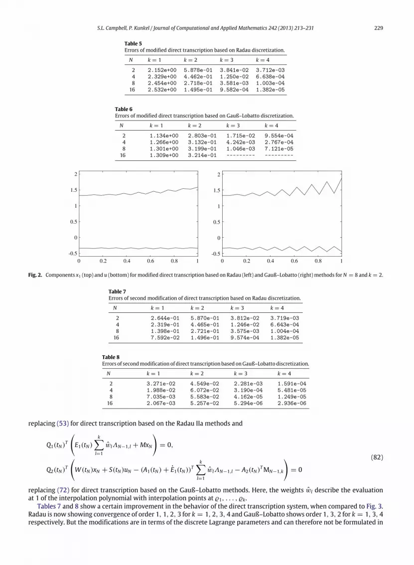
Tables 5 and 6 show some improvement in the behavior but the results are still not very satisfactory. The missing valuesin Table 6 for N = 16 are due to a numerical rank deficiency of the Jacobian. For Radau we are now seeing convergence fork = 2, 3, 4 that appears to be approaching k − 1. For Gauß–Lobatto we have order 2 for k = 3, 4.

Fig. 2 suggests that there is a problem with the boundary condition at the right boundary. Thus, we applied a secondmodification of the direct transcription system with

Q1(tN)T (E(tN)ΛN−1,k + MxN) = 0,

Q2(tN)T (W (tN)xN + S(tN)uN − (A(tN) + E(tN))TΛN−1,k) = 0,(81)


Table 5Errors of modified direct transcription based on Radau discretization.

N k = 1 k = 2 k = 3 k = 4

2 2.152e+00 5.878e-01 3.841e-02 3.712e-034 2.329e+00 4.462e-01 1.250e-02 6.638e-048 2.454e+00 2.718e-01 3.581e-03 1.003e-04

16 2.532e+00 1.495e-01 9.582e-04 1.382e-05

Table 6Errors of modified direct transcription based on Gauß–Lobatto discretization.

N k = 1 k = 2 k = 3 k = 4

2 1.134e+00 2.803e-01 1.715e-02 9.554e-044 1.266e+00 3.132e-01 4.242e-03 2.767e-048 1.301e+00 3.199e-01 1.046e-03 7.121e-05

16 1.309e+00 3.214e-01 --------- ---------

-0.5

0

0.5

1

1.5

2

0 0.2 0.4 0.6 0.8 1-0.5

0

0.5

1

1.5

2

0 0.2 0.4 0.6 0.8 1

Fig. 2. Components x1 (top) and u (bottom) formodified direct transcription based on Radau (left) and Gauß–Lobatto (right) methods forN = 8 and k = 2.

Table 7Errors of second modification of direct transcription based on Radau discretization.

N k = 1 k = 2 k = 3 k = 4

2 2.644e-01 5.870e-01 3.812e-02 3.719e-034 2.319e-01 4.465e-01 1.246e-02 6.643e-048 1.398e-01 2.721e-01 3.575e-03 1.004e-04

16 7.592e-02 1.496e-01 9.574e-04 1.382e-05

Table 8Errors of secondmodification of direct transcription based onGauß–Lobatto discretization.

N k = 1 k = 2 k = 3 k = 4

2 3.271e-02 4.549e-02 2.281e-03 1.591e-044 1.988e-02 6.072e-02 3.190e-04 5.481e-058 7.035e-03 5.583e-02 4.162e-05 1.249e-05

16 2.067e-03 5.257e-02 5.294e-06 2.936e-06

replacing (53) for direct transcription based on the Radau IIa methods and

Q1(tN)T

E1(tN)

kl=1

wlΛN−1,l + MxN

= 0,

Q2(tN)T

W (tN)xN + S(tN)uN − (A1(tN) + E1(tN))T

kl=1

wlΛN−1,l − A2(tN)TMN−1,k

= 0

(82)

replacing (72) for direct transcription based on the Gauß–Lobatto methods. Here, the weights wl describe the evaluationat 1 of the interpolation polynomial with interpolation points at ϱ1, . . . , ϱk.

Tables 7 and 8 show a certain improvement in the behavior of the direct transcription system, when compared to Fig. 3.Radau is now showing convergence of order 1, 1, 2, 3 for k = 1, 2, 3, 4 and Gauß–Lobatto shows order 1, 3, 2 for k = 1, 3, 4respectively. But the modifications are in terms of the discrete Lagrange parameters and can therefore not be formulated in


-0.5

0

0.5

1

1.5

0.5

1.5

2

0 0.2 0.4 0.6 0.8 0.2 0.4 0.6 0.81-0.5

0

1

2

0 1

Fig. 3. Components x1 (top) and u (bottom) for second modification of direct transcription based on Radau (left) and Gauß–Lobatto (right) methods forN = 8 and k = 2.

terms of a discrete optimization problem beforehand. Moreover, in view of the results for the discretization of the necessaryboundary value problem, the results for direct transcription are still not satisfactory.

6. Conclusion

In interpreting order results for optimal control problems it is important to keep in mind that in practice they aredependent on the smoothness of the problem. In applications there are sometimes limitations on the smoothness thatis available. For example, functions in the dynamics may come from measured data directly or by interpolation. Controland state constraints can create discontinuities in the control or its derivative. If problem smoothness is known, then theboundary value solution seems much more efficient. However, if the boundary value problem is more complex or there isnot the needed smoothness and a direct transcription approach is attempted the Radau discretization appears better basedon the tests here.

It has been observed for other discretizations with ODE dynamics that the necessary conditions for the discretization aresometimes a numerical approximation of a transformed version of the necessary conditions for the continuous problem [14].We have applied direct transcription using the two discretizations discussed here to a DAE with constant leading term butwhich is not semi-explicit. Without any modifications we again saw reduced order for both methods. However, with thefirst modification we saw no order reduction for either Radau or Gauss–Lobatto. But as noted there was still order reductionin the time-varying coefficient case.

We see then that there are two effects going on creating reduction. One has to do with the fact that modifications areneeded to the solution of the discrete necessary conditions to have any hope of high order on problems that are not semi-explicit. However, even if that is done, as we have shown here, a leading coefficient with varying nullspace can still resultin order reduction even for the modified problem.

References

[1] K.E. Brenan, S.L. Campbell, L.R. Petzold, Numerical Solution of Initial-Value Problems in Differential-Algebraic Equations, in: Classics in AppliedMathematics, vol. 14, SIAM, Philadelphia, PA, 1996.

[2] P. Kunkel, V. Mehrmann, Differential-Algebraic Equations — Analysis and Numerical Solution, EMS Publishing House, Zürich, Switzerland, 2006.[3] J.T. Betts, Practical Methods for Optimal Control and Estimation using Nonlinear Programming, second ed., Society for Industrial and Applied

Mathematics, Philadelphia, PA, 2010.[4] L. Dai, Singular Control Systems, Springer-Verlag, Berlin, Germany, 1989.[5] A. Kumar, P. Daoutidis, Control of Nonlinear Differential Algebraic Equation Systems with Applications to Chemical Processes, in: Research Notes in

Mathematics, Pitman, 1999.[6] U.M. Ascher, R.J. Spiteri, Collocation software for boundary value differential-algebraic equations, SIAM Journal on Scientific Computing 15 (1994)

938–952.[7] J.T. Betts, Trajectory optimization in the presence of uncertainty, The Journal of the Astronautical Sciences 54 (2) (2006) 227–243.[8] N. Biehn, S.L. Campbell, L. Jay, T. Westbrook, Some comments on DAE theory for IRK methods and trajectory optimization, Journal of Computational

and Applied Mathematics 120 (2000) 109–131.[9] H.G. Bock, K.J. Plitt, A multiple shooting algorithm for direct solution of optimal control problems, in: Proceedings of the 9th IFAC World Congress,

Pergamon Press, Budapest, Hungary, 1984, pp. 242–247.[10] P.J. Enright, B.A. Conway, Discrete approximations to optimal trajectories using direct transcription and nonlinear programming, AIAA Journal of

Guidance, Control, and Dynamics 15 (4) (1992) 994–1002.[11] M. Gerdts, Local minimum principle for optimal control problems subject to differential-algebraic equations of index two, Journal of Optimization

Theory and Applications 130 (2006) 441–460.[12] M. Gerdts, Direct shooting method for the numerical solution of higher-index DAE optimal control problems, Journal of Optimization Theory and

Applications 117 (2) (2003) 267–294.[13] W.W. Hager, Numerical analysis in optimal control, in: Conference on Optimal Control of Complex Structures, in: International Series of Numerical

Mathematics, vol. 139, Birkhauser Verlag, Basel, Switzerland, 2001, pp. 83–93.[14] W.W. Hager, Runge–Kutta methods in optimal control and the transformed adjoint system, Numerische Mathematik 87 (2000) 247–282.[15] A.L. Herman, B.A. Conway, Direct optimization using collocation based on high-Order Gauss–Lobatto quadrature rules, AIAA Journal of Guidance,

Control, and Dynamics 19 (3) (1996) 592–599.


[16] J.S. Logsdon, L.T. Biegler, Accurate solution of differential-algebraic optimization problems, Industrial Engineering Chemical Research 28 (11) (1989)1628–1639.

[17] V.H. Schulz, H.G. Bock, M.C. Steinbach, Exploiting invariants in the numerical solution of multipoint boundary value problems for DAE, SIAM Journalon Scientific Computing 19 (1998) 440–467.

[18] R. Stöver, Collocation methods for solving linear differential-algebraic boundary value problems, Numerische Mathematik 88 (2001) 771–795.[19] O. von Stryk, Numerical solution of optimal control problems by direct collocation, in: Roland Bulirsch, Angelo Miele, Josef Stoer, Klaus H. Well (Eds.),

Optimal Control, in: International Series of Numerical Mathematics, vol. 111, Birkhäuser Verlag, Basel, 1993, pp. 129–143.[20] O. von Stryk, R. Bulirsch, Direct and indirect methods for trajectory optimization, Annals of Operations Research 37 (1992) 357–373.[21] A. Engelsone, S.L. Campbell, J.T. Betts, Direct transcrition solution of higher-index optimal control problems and the virtual index, Applied Numerical

Mathematics 57 (2007) 281–296.[22] S. Kameswaran, L.T. Biegler, Simultaneous dynamic optimization strategies: recent advances and challenges, Computers and Chemical Engineering

30 (2006) 1560–1575.[23] P. Kunkel, V. Mehrmann, Optimal control for unstructured nonlinear differential-algebraic equations of arbitrary index, Mathematics of Control,

Signals, and Systems 20 (2008) 227–269.[24] E. Hairer, G. Wanner, Solving Ordinary Differential Equations II, Springer-Verlag, Berlin, 1991.[25] P. Kunkel, V. Mehrmann, R. Stöver, Symmetric collocation for unstructured nonlinear differential-algebraic equations of arbitrary index, Numerische

Mathematik 91 (2004) 475–501.[26] S.L. Campbell, A general form for solvable linear time varying singular systems of differential equations, SIAM Journal of Mathematical Analysis 18

(1987) 1101–1115.[27] S.L. Campbell, C.D. Meyer, Generalized Inverses of Linear Transformations, in: SIAM Classics, SIAM, Philadelphia, 2009.[28] A. Backes, Optimale Steuerung der linearen DAE im fall index 2. Dissertation, Mathematisch-Naturwissenschaftliche Fakultät, Humboldt-Universität

zu Berlin, Berlin, Germany, 2006.

Documents

On the numerical treatment of linear–quadratic optimal control problems for general linear time-varying differential-algebraic equations