Optimal Control Using an Algebraic Method forControl-Affine Nonlinear Systems

Chang-Hee Won and Saroj BiswasDepartment of Electrical and Computer Engineering

Temple University1947 N. 12th Street

Philadelphia, PA 19122Voice (215) 204-6158, Fax (215) 204-5960cwon@temple.edu, sbiswas@temple.edu

April 20, 2007

Abstract

A deterministic optimal control problem is solved for a control-affine nonlin-

ear system with a nonquadratic cost function. We algebraically solve the Hamilton-

Jacobi equation for the gradient of the value function. This eliminates the need to

explicitly solve the solution of a Hamilton-Jacobi partial differential equation. We

interpret the value function in terms of the control Lyapunov function. Then we

provide the stabilizing controller and the stability margins. Furthermore, we derive

an optimal controller for a control-affine nonlinear system using the state dependent

Riccati equation (SDRE) method; this method gives a similar optimal controller as

the controller from the algebraic method. We also find the optimal controller when

the cost function is the exponential-of-integral case, which is known as risk-sensitive

(RS) control. Finally, we show that SDRE and RS methods give equivalent optimal

controllers for nonlinear deterministic systems. Examples demonstrate the proposed

methods.

1

Keywords: Optimal Control, Hamilton-Jacobi Equation, Control-Affine Nonlinear

System, Nonquadratic Cost, Algebraic Method

1 Introduction

A number of researchers have worked on the nonlinear optimal control problem,

but they usually assume a linear system with a quadratic form of the cost function

[3, 8, 9]. For example, Glad used a quadratic form of the cost function with higher

order terms [8]. Here, we consider a cost function which is quadratic in control

action but nonquadratic with respect to the states. Also, we consider the affine-

control nonlinear system that is linear in control action but nonlinear in terms of the

state. Then we derive the Hamilton-Jacobi (HJ) partial differential equation. A major

challenge in nonlinear optimal control is in solving this HJ partial differential equation.

We solve the HJ equation by viewing the HJ equation as an algebraic equation and

solve for the gradient of the cost function. The optimal controller is found using

the gradient of the cost function. By converting the HJ partial differential equation

problems into the algebraic equation problems, we can solve HJ partial differential

equation more easily. Obtaining an optimal controller using the partial derivative

of the cost function has been discussed in the literature. For example, see [15]. In

our formulation, however, we go a step further and algebraically solve the gradient

2

of the cost function in terms of the system parameters and weighting functions. In

this paper, we consider a nonlinear deterministic system and optimize a nonquadratic

cost function.

Recently, the control Lyapunov function is generating renewed interest in non-

linear optimal control. We investigate the stability and robustness properties of the

optimal controller using a control Lyapunov function. In 2000, Primbs et al. solved

nonlinear control problems using a new class of receding horizon control and control

Lyapunov function [13]. This control scheme heuristically relates pointwise min-norm

control with receding horizon control, and it does not analytically solve nonlinear op-

timal control problems. In 2004, Curtis and Beard solved a nonlinear control problem

using the satisficing sets and control Lyapunov function [4]. This framework com-

pletely characterizes all universal formulas, but they have two utility functions that

quantify the benefits and costs of an action, which is different from traditional op-

timal control cost function. In this paper, we solve a unconstrained optimal control

problem with nonquadratic cost function for a deterministic affine-control nonlinear

system.

Two other methods of dealing with the nonlinear optimal control problems are

State Dependent Riccati Equation (SDRE) method [3] and risk-sensitive control

method [9, 16]. The SDRE methods solve a nonlinear optimal control problem

through a Riccati equation that depends on the state. The method seems to work well

in applications but rigorous theoretical proofs are lacking in this area. The authors

3

will derive SDRE and the optimal controller using Kronecker products. An example

demonstrates that we obtain a similar optimal controller as our optimal controller

obtained through the algebraic method. The risk-sensitive control method is an opti-

mal control method that assumes an exponential of the quadratic cost function. For a

linear deterministic system, the linear quadratic regulator problem and risk-sensitive

control problem provide same optimal controller. In this paper, we show that the

risk-sensitive controller is equivalent to the SDRE controller for a special nonlinear

system. Thus, we show that there is a close relationship between the optimal control

using the algebraic, SDRE, and risk-sensitive methods. The preliminary version of

the current paper was presented in [17].

In the next section, we derive the optimal full-state-feedback solution of a deter-

ministic affine nonlinear system. In Subsection 2.1, we interpret the stability and

robustness of the optimal controller by relating control Lyapunov function (clf) in-

equality to the HJ equation. In Sections 3 and 4, two other nonlinear optimal control

methods are discussed; the state dependent Riccati Equation (SDRE) method and

risk-sensitive control method. Here, we derive the SDRE controller for a nonlinear

system for a quadratic form cost function. Finally, risk-sensitive control law is derived

for a nonlinear deterministic system.

4

2 Hamilton-Jacobi Equation and Optimal Controller

Consider the following nonlinear system, which is linear in the control action but

nonlinear with respect to the state.

dx(t)

dt= g(x(t)) + B(x(t))u(t), x(0) = x0 (1)

where g : IRn → IRn, B : IRn → IRn×m, x ∈ IRn, and u ∈ U = IRm. By a control,

we mean any U valued, Lebesgue measurable function u on (0,∞) for any t < ∞.

Assume that g and B are continuously differentiable in x. Furthermore, consider

the following nonquadratic infinite-time cost function, which is quadratic in control

action but nonquadratic with respect to the state,

J(x, u) =∫

∞

0

[l(x) + u′R(x)u]dτ, (2)

where l(x) is continuously differentiable and nonnegative definite, R(x) is symmetric

and positive definite for all x 6= 0, and ′ denotes transposition. We also assume

that [g(x), l(x)] is zero-state detectable. The optimization problem is to design a

state-feedback controller that will minimize the cost function, Eq. (2), subject to (1).

Assuming that there exists a twice continuously differentiable (C2), V : IRn → IR+, we

obtain the following Hamilton Jacobi (HJ) equation [5] using dynamic programming

method.

1

4

∂V (x)

∂x

′

B(x)R−1(x)B′(x)∂V (x)

∂x− g′(x)

∂V (x)

∂x− l(x) = 0. (3)

It is well known that the value functions are not necessarily continuously differen-

tiable. So, this C2 assumption is a first step toward solving the full-state-feedback

5

control problem. For the above HJ equation, with differentiability and a nonnegative

definiteness assumptions, the optimal controller can be found as

u∗ = −1

2R−1(x)B′(x)

∂V (x)

∂x. (4)

Here we note that∂V (x)

∂xis a column vector. By the positive definite assumption of

R(x) in the cost function, Eq. (2), the inverse of R(x) exists for all x 6= 0. Therefore,

the controller is a candidate for an optimal controller.

Here, instead of finding V from the HJ equation, we will determine an explicit

expression for∂V (x)

∂x. To find the optimal controller we introduce a generalized

version of the lemma by Liu and Leake [12, 14]. Our version generalizes the Lemma

to include positive semi-definite matrices by using pseudo-inverse (Moore-Penrose

generalized inverse).

Lemma 2.1 Let x ∈ IRn be a real n-vector, z(x) and y(x) be real r-vector functions,

and α(x) be a real function defined on IRn. Let X be a positive semi-definite and

symmetric real matrix. Then z(x) satisfies the condition

z′(x)Xz(x) + 2z′(x)y(x) + α(x) = 0 (5)

if and only if

y′(x)X+y(x) ≥ α(x), (6)

where X+ is the pseudo-inverse of X. In this case, the set of all solutions to (5) is

represented by

z(x) = −X+y(x) + H+a(x)β(x) (7)

6

where

β(x) =(

y′(x)X+y(x) − α(x))

1

2 . (8)

Let H be a square matrix, such that X = H ′H, and a(x) is an arbitrary unit vector.

We assume that a(x), z(x) are images of H for all x.

Proof. The sufficiency is shown by direct substitution. Suppressing the arguments

and substituting Eq. (7) into Eq. (5) gives

(−y′X+ + β ′a′H+′

)X(−X+y + H+aβ) + 2(−y′X+ + β ′a′H+′

)y + α = 0.

After some manipulations we obtain

y′X+y − 2β ′a′H+′

XX+y − β ′a′H+′

XH+aβ − 2y′X+y + 2β ′a′H+′

y + α = 0.

We used the pseudo-inverse property, X+XX+ = X+. The second term on the left

side of the equality is rewritten as −2β ′a′H+′

H ′H(H ′H)+y. Then we use pseudo-

inverse properties A′+ = A+′

and HH+a = a for any vector a which is an image of H

[11, p. 434]. We also use the assumption that a is an image of H . So, the second term

on the left hand side, now becomes −2β ′(HH+a)′HH+H ′+y = −2β ′a′HH+H+′

y =

−2β ′(H+′

H ′a)′H+′

y = −2β ′a′H+′

y. Thus, it cancels with the fifth term on the left

hand side. Now we obtain

−y′X+y + α − β ′a′H+′

XH+aβ = 0. (9)

Now, we consider the third term on the left hand side of the above equation. Because

we assumed that a(x) is an image of H , we have H+′

XH+ = H+′

H ′HH+ = I. Thus,

7

the third term on the left hand side of Eq. (9) becomes β ′a′aβ. We reduce Eq. (9)

into

−y′X+y + α − β ′β = 0.

By substituting Eq. (8) into the above equation, we establish the sufficiency.

To show the conditions are necessary, we change the variables z = Hz and y =

(H+)′y. Then we note that y′X+y = |y|2 < α implies

|z + y|2 < 0,

which is a contradiction. Let w = z + y, then using Eq. (8), we note that (5) implies

w′w = β2. Take a =w

|w| , we have w = aβ. Substituting the variables back we have

z + y = aβ

Hz + (H+)′y = aβ

Hz = −(H+)′y + aβ

z = −(H ′H)+y + H+aβ.

In the last step we used the assumption that z is an image of H . Consequently, (7)

follows. 2

Remark 2.1 This lemma gives a quadratic formula for the vectors.

Now, we present the following corollary for positive definite X, which follows from

the above lemma. This is the lemma that was given by Liu and Leake [12, 14].

8

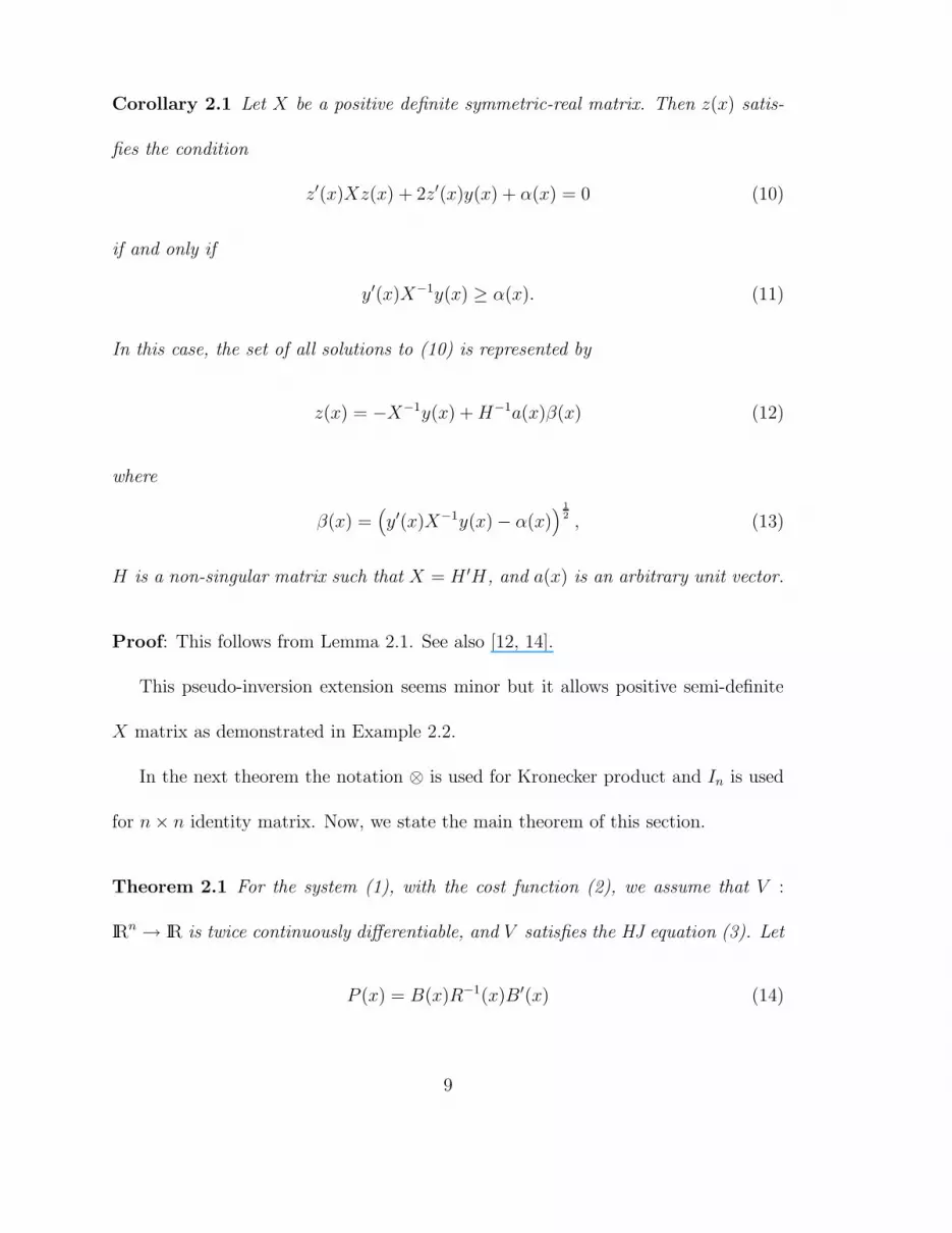
Corollary 2.1 Let X be a positive definite symmetric-real matrix. Then z(x) satis-

fies the condition

z′(x)Xz(x) + 2z′(x)y(x) + α(x) = 0 (10)

if and only if

y′(x)X−1y(x) ≥ α(x). (11)

In this case, the set of all solutions to (10) is represented by

z(x) = −X−1y(x) + H−1a(x)β(x) (12)

where

β(x) =(

y′(x)X−1y(x) − α(x))

1

2 , (13)

H is a non-singular matrix such that X = H ′H, and a(x) is an arbitrary unit vector.

Proof: This follows from Lemma 2.1. See also [12, 14].

This pseudo-inversion extension seems minor but it allows positive semi-definite

X matrix as demonstrated in Example 2.2.

In the next theorem the notation ⊗ is used for Kronecker product and In is used

for n × n identity matrix. Now, we state the main theorem of this section.

Theorem 2.1 For the system (1), with the cost function (2), we assume that V :

IRn → IR is twice continuously differentiable, and V satisfies the HJ equation (3). Let

P (x) = B(x)R−1(x)B′(x) (14)

9

and

ρ(x) =√

P (x)a(x)√

g′(x)P+(x)g(x) + l(x), (15)

where a(x) is an arbitrary unit vector. For an affine nonlinear system (1), the optimal

controller that minimizes the cost function (2) is given by

u∗(x) = −R−1(x)B′(x)P+(x) [g(x) + ρ(x)] , (16)

if the following symmetry, non-negative definite, and image requirements are satisfied.

P+

(

∂g

∂x′+

∂ρ

∂x′

)

+∂P+

∂x′(In ⊗ (g + ρ)) =

(

∂g

∂x′+

∂ρ

∂x′

)

′

P+ + (In ⊗ (g + ρ))′(

∂P+

∂x′

)

′

,

(17)

P+

(

∂g

∂x′+

∂ρ

∂x′

)

+∂P+

∂x′(In ⊗ (g + ρ)) ≥ 0, (18)

and

a(x) and∂V (x)

∂xare images of

√

B(x)R−1(x)B′(x)/2 for all x. (19)

Proof. Utilizing Lemma 2.1 on Eq. (3) with z =∂V

∂x, X = (BR−1B′/4), y =

−g/2, and α = −l, we have

∂V

∂x= −1

2

(

1

4BR−1B′

)+

(−g) +

√

(

1

4BR−1B′

)+

a

√

1

4g′

(

1

4BR−1B′

)+

g + l

= 2(BR−1B′)+g + 2√

(BR−1B′)+a√

g′ (BR−1B′)+ g + l. (20)

We let H =√

B(x)R−1(x)B′(x)/2. From Eq. (4), the optimal controller is given as

u∗ = −R−1B′(BR−1B′)+g − R−1B′

√

(BR−1B′)+a√

g′ (BR−1B′)+ g + l

= −R−1B′(BR−1B′)+

[

g +√

BR−1B′a√

g′ (BR−1B′)+ g + l]

, (21)

10

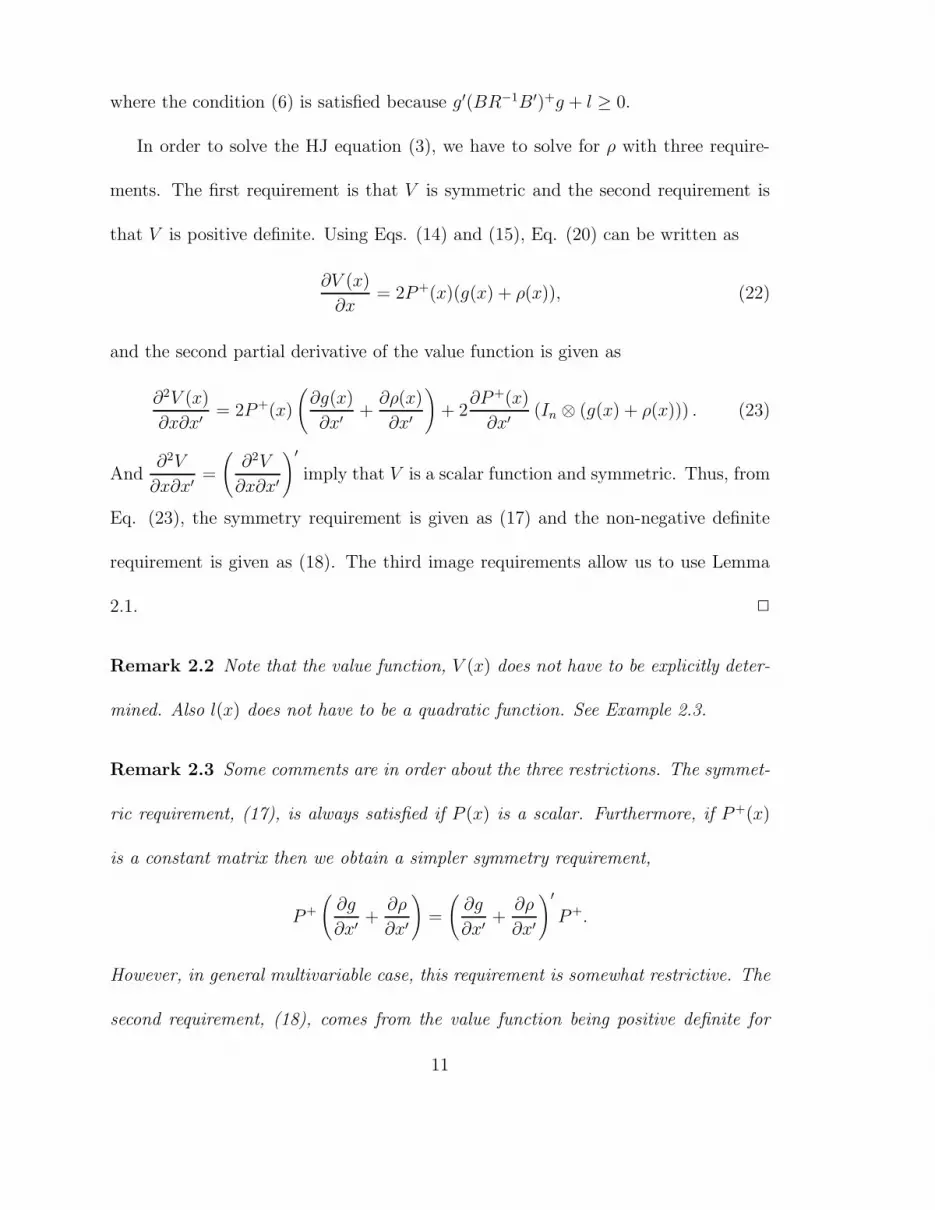
where the condition (6) is satisfied because g′(BR−1B′)+g + l ≥ 0.

In order to solve the HJ equation (3), we have to solve for ρ with three require-

ments. The first requirement is that V is symmetric and the second requirement is

that V is positive definite. Using Eqs. (14) and (15), Eq. (20) can be written as

∂V (x)

∂x= 2P+(x)(g(x) + ρ(x)), (22)

and the second partial derivative of the value function is given as

∂2V (x)

∂x∂x′= 2P+(x)

(

∂g(x)

∂x′+

∂ρ(x)

∂x′

)

+ 2∂P+(x)

∂x′(In ⊗ (g(x) + ρ(x))) . (23)

And∂2V

∂x∂x′=

(

∂2V

∂x∂x′

)

′

imply that V is a scalar function and symmetric. Thus, from

Eq. (23), the symmetry requirement is given as (17) and the non-negative definite

requirement is given as (18). The third image requirements allow us to use Lemma

2.1. 2

Remark 2.2 Note that the value function, V (x) does not have to be explicitly deter-

mined. Also l(x) does not have to be a quadratic function. See Example 2.3.

Remark 2.3 Some comments are in order about the three restrictions. The symmet-

ric requirement, (17), is always satisfied if P (x) is a scalar. Furthermore, if P+(x)

is a constant matrix then we obtain a simpler symmetry requirement,

P+

(

∂g

∂x′+

∂ρ

∂x′

)

=

(

∂g

∂x′+

∂ρ

∂x′

)

′

P+.

However, in general multivariable case, this requirement is somewhat restrictive. The

second requirement, (18), comes from the value function being positive definite for

11

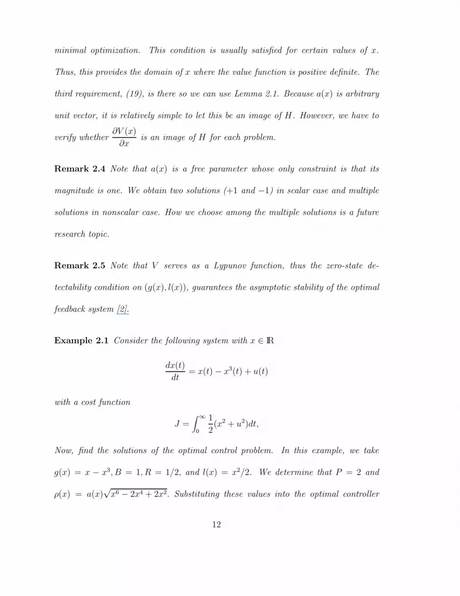
minimal optimization. This condition is usually satisfied for certain values of x.

Thus, this provides the domain of x where the value function is positive definite. The

third requirement, (19), is there so we can use Lemma 2.1. Because a(x) is arbitrary

unit vector, it is relatively simple to let this be an image of H. However, we have to

verify whether∂V (x)

∂xis an image of H for each problem.

Remark 2.4 Note that a(x) is a free parameter whose only constraint is that its

magnitude is one. We obtain two solutions (+1 and −1) in scalar case and multiple

solutions in nonscalar case. How we choose among the multiple solutions is a future

research topic.

Remark 2.5 Note that V serves as a Lypunov function, thus the zero-state de-

tectability condition on (g(x), l(x)), guarantees the asymptotic stability of the optimal

feedback system [2].

Example 2.1 Consider the following system with x ∈ IR

dx(t)

dt= x(t) − x3(t) + u(t)

with a cost function

J =∫

∞

0

1

2(x2 + u2)dt,

Now, find the solutions of the optimal control problem. In this example, we take

g(x) = x − x3, B = 1, R = 1/2, and l(x) = x2/2. We determine that P = 2 and

ρ(x) = a(x)√

x6 − 2x4 + 2x2. Substituting these values into the optimal controller

12

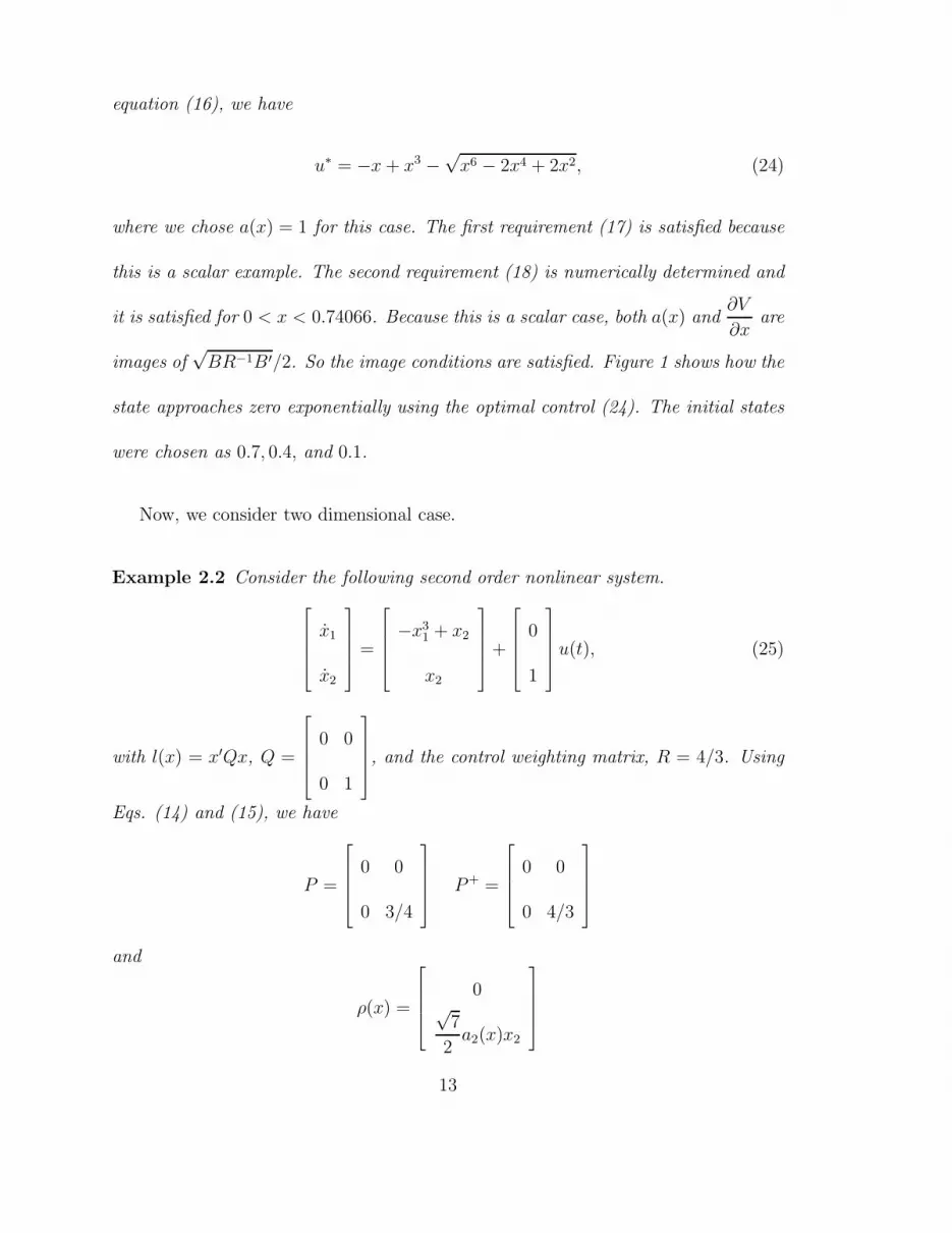
equation (16), we have

u∗ = −x + x3 −√

x6 − 2x4 + 2x2, (24)

where we chose a(x) = 1 for this case. The first requirement (17) is satisfied because

this is a scalar example. The second requirement (18) is numerically determined and

it is satisfied for 0 < x < 0.74066. Because this is a scalar case, both a(x) and∂V

∂xare

images of√

BR−1B′/2. So the image conditions are satisfied. Figure 1 shows how the

state approaches zero exponentially using the optimal control (24). The initial states

were chosen as 0.7, 0.4, and 0.1.

Now, we consider two dimensional case.

Example 2.2 Consider the following second order nonlinear system.

x1

x2

=

−x31 + x2

x2

+

0

1

u(t), (25)

with l(x) = x′Qx, Q =

0 0

0 1

, and the control weighting matrix, R = 4/3. Using

Eqs. (14) and (15), we have

P =

0 0

0 3/4

P+ =

0 0

0 4/3

and

ρ(x) =

0√

7

2a2(x)x2

13

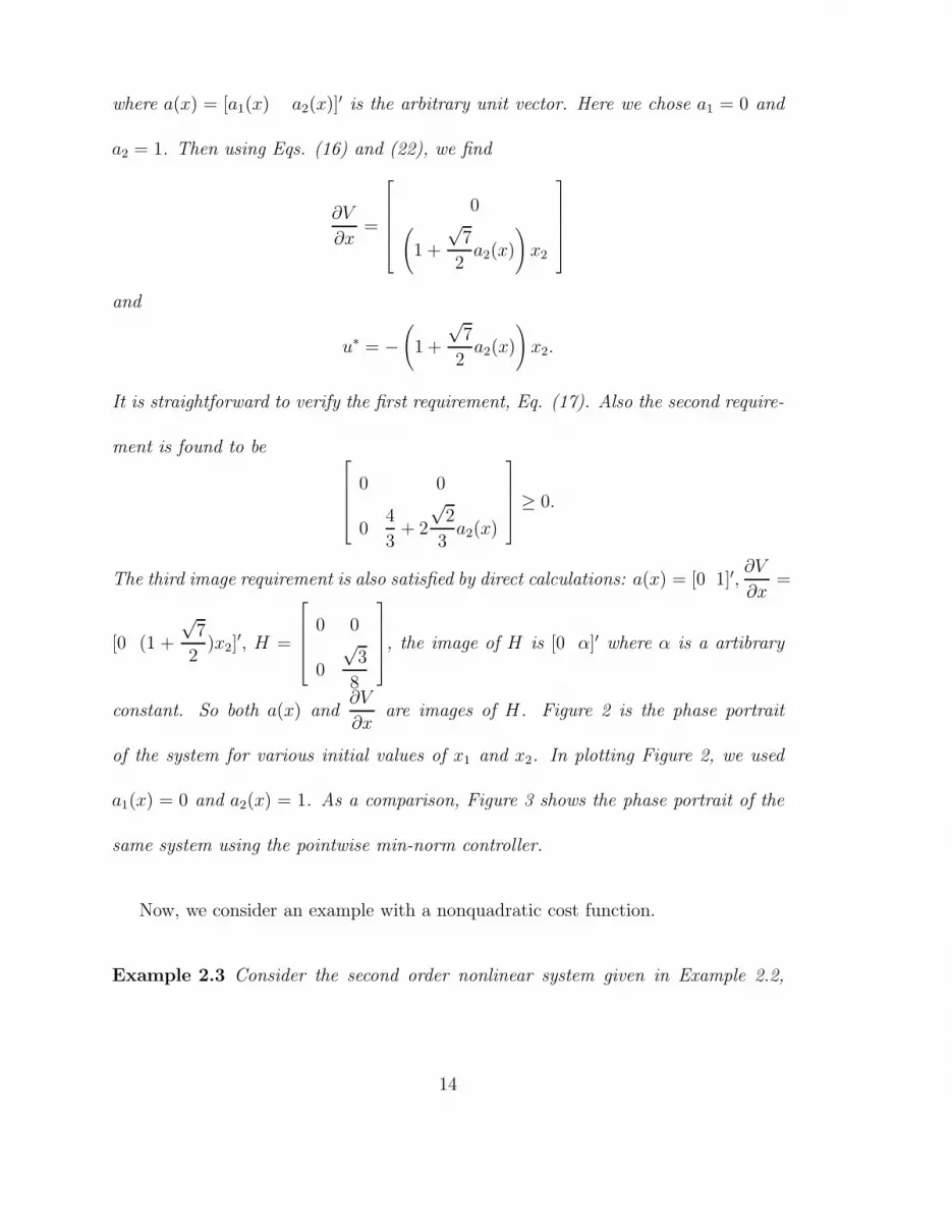
where a(x) = [a1(x) a2(x)]′ is the arbitrary unit vector. Here we chose a1 = 0 and

a2 = 1. Then using Eqs. (16) and (22), we find

∂V

∂x=

0(

1 +

√7

2a2(x)

)

x2

and

u∗ = −(

1 +

√7

2a2(x)

)

x2.

It is straightforward to verify the first requirement, Eq. (17). Also the second require-

ment is found to be

0 0

04

3+ 2

√2

3a2(x)

≥ 0.

The third image requirement is also satisfied by direct calculations: a(x) = [0 1]′,∂V

∂x=

[0 (1 +

√7

2)x2]

′, H =

0 0

0

√3

8

, the image of H is [0 α]′ where α is a artibrary

constant. So both a(x) and∂V

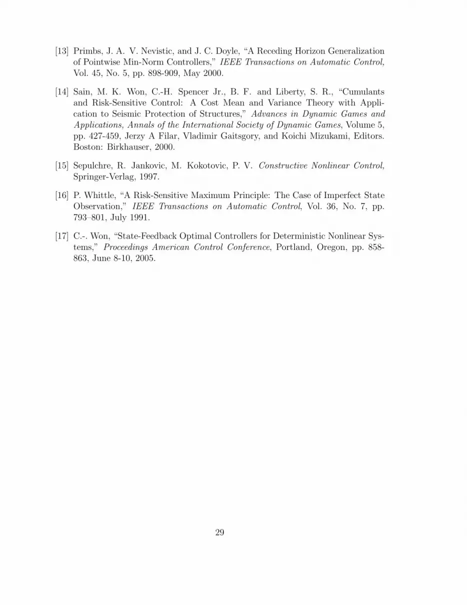
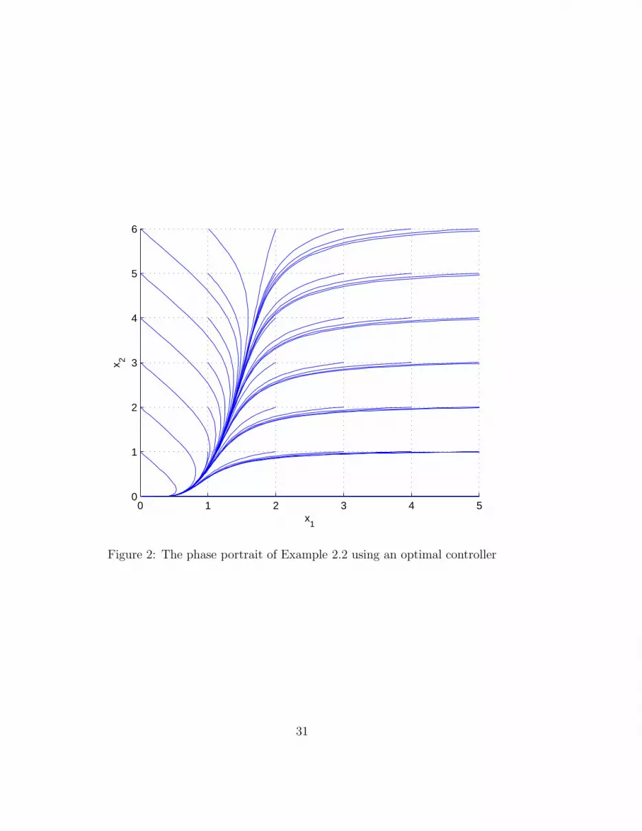
∂xare images of H. Figure 2 is the phase portrait

of the system for various initial values of x1 and x2. In plotting Figure 2, we used

a1(x) = 0 and a2(x) = 1. As a comparison, Figure 3 shows the phase portrait of the

same system using the pointwise min-norm controller.

Now, we consider an example with a nonquadratic cost function.

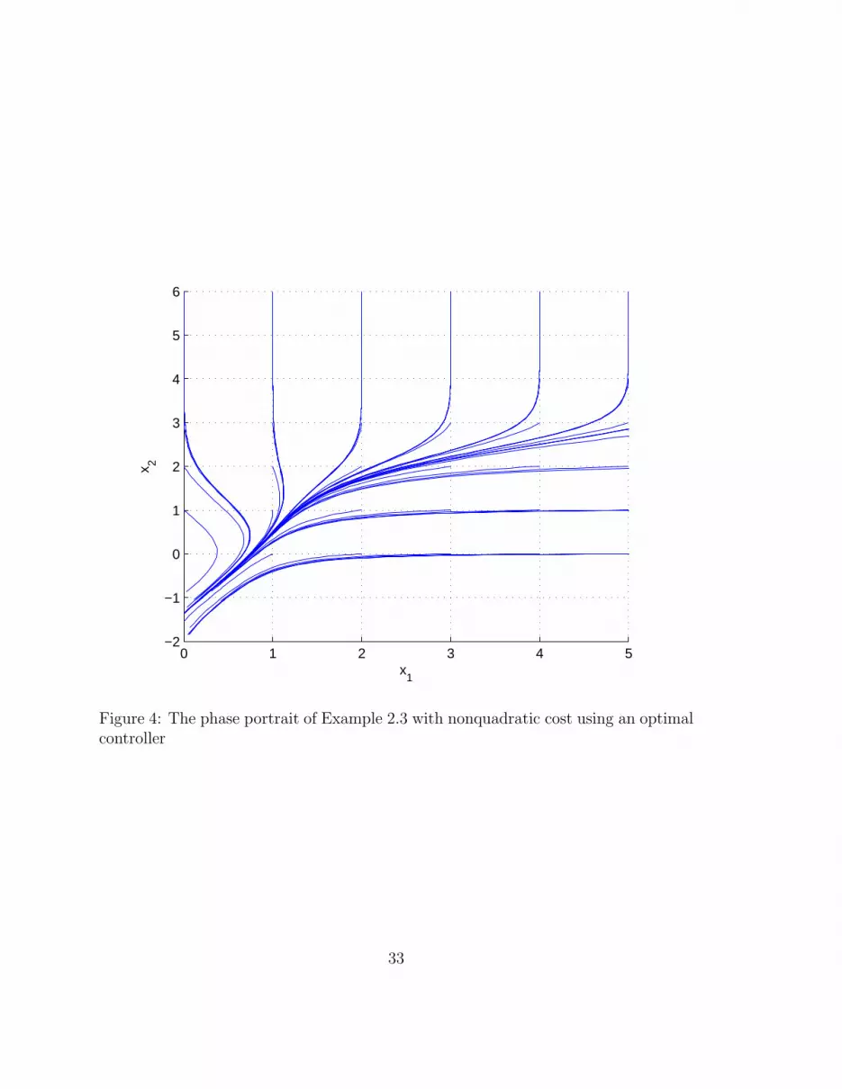
Example 2.3 Consider the second order nonlinear system given in Example 2.2,

14

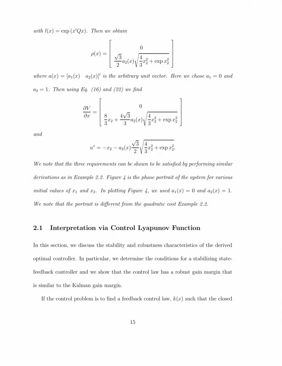
with l(x) = exp (x′Qx). Then we obtain

ρ(x) =

0√

3

2a2(x)

√

4

3x2

2 + exp x22

where a(x) = [a1(x) a2(x)]′ is the arbitrary unit vector. Here we chose a1 = 0 and

a2 = 1. Then using Eq. (16) and (22) we find

∂V

∂x=

0

8

3x2 +

4√

3

3a2(x)

√

4

3x2

2 + exp x22

and

u∗ = −x2 − a2(x)

√3

2

√

4

3x2

2 + exp x22.

We note that the three requirements can be shown to be satisfied by performing similar

derivations as in Example 2.2. Figure 4 is the phase portrait of the system for various

initial values of x1 and x2. In plotting Figure 4, we used a1(x) = 0 and a2(x) = 1.

We note that the portrait is different from the quadratic cost Example 2.2.

2.1 Interpretation via Control Lyapunov Function

In this section, we discuss the stability and robustness characteristics of the derived

optimal controller. In particular, we determine the conditions for a stabilizing state-

feedback controller and we show that the control law has a robust gain margin that

is similar to the Kalman gain margin.

If the control problem is to find a feedback control law, k(x) such that the closed

15

loop system

x = f(x, k(x)) (26)

is asymptotically stable at the equilibrium point x = 0, then we can choose a function

V (x) as a Lyapunov function, and find k(x) to guarantee that for all x ∈ IRn such

that

∂V (x)

∂x

′

(g(x) + B(x)k(x)) ≤ −W (x). (27)

A system for which an appropriate choice of V (x) and W (x) exists is said to possess

a control Lyapunov function (clf). Following [10] we define the control Lyapunov

function, V (x), of system (26) to be smooth, positive definite, and radially unbounded

if

infu

{

∂V

∂xf(x, u)

}

< 0, (28)

for all x not equal to zero.

In order to relate the clf inequality to the HJ equation of the optimal control, we

introduce the following lemma by Curtis and Beard with a slight modification [4].

Lemma 2.2 If S = S ′ > 0 then the set of solutions to the quadratic inequality

ζ ′Sζ + d′ζ + c ≤ 0 (29)

where ζ ∈ IRn is nonempty if and only if

1

4d′S−1d − c ≥ 0 (30)

and is given by

ζ = −1

2S−1d + S−1/2v

√

1

4d′S−1d − c (31)

16

where v ∈ B(IRn) = {ζ ∈ IRn : ‖ζ‖ ≤ 1}.

Proof. See [4], and modify the inequalities.

Now, we state the theorem that gives all stabilizing controller.

Theorem 2.2 For the system (1), with the cost function (2), we assume that V

satisfies the HJ equation (3). We also assume that V (x) is C2, positive definite, and

radially unbounded function. Moreover, we assume W (x) = l(x)+k′(x)R(x)k(x). All

state-feedback stabilizing controllers for the assumed form of W are given by

k = −1

2R−1B′

∂V

∂x+ R−1/2v

√

1

4

∂V

∂x

′

BR−1B′∂V

∂x− g′

∂V

∂x− l (32)

if and only if

1

4

∂V

∂x

′

BR−1B′∂V

∂x− g′

∂V

∂x− l ≥ 0. (33)

Proof. From (27), we obtain the control Lyapunov function inequality as

∂V

∂x

′

(g + Bk) + l + k′Rk ≤ 0. (34)

Then we let ζ = k, S = R, d = B′∂V

∂x, and c = g′

∂V

∂x+ l and use Lemma 2.2 on Eq.

(34), to obtain all the stabilizing controller. 2

Remark 2.6 Following [4], we can also show that k(x) in Eq. (32) is inversely

optimal for some R(x) and l(x).

Here we discuss the robustness property of the optimal controller. We follow the

definition of the stability margin given in [4]: an asymptotically stabilizing control

17

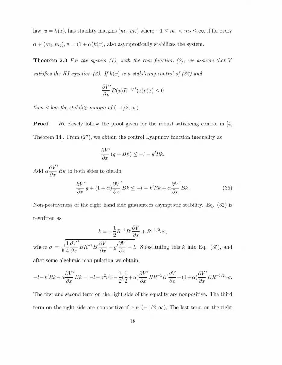
law, u = k(x), has stability margins (m1, m2) where −1 ≤ m1 < m2 ≤ ∞, if for every

α ∈ (m1, m2), u = (1 + α)k(x), also asymptotically stabilizes the system.

Theorem 2.3 For the system (1), with the cost function (2), we assume that V

satisfies the HJ equation (3). If k(x) is a stabilizing control of (32) and

∂V

∂x

′

B(x)R−1/2(x)v(x) ≤ 0

then it has the stability margin of (−1/2,∞).

Proof. We closely follow the proof given for the robust satisficing control in [4,

Theorem 14]. From (27), we obtain the control Lyapunov function inequality as

∂V

∂x

′

(g + Bk) ≤ −l − k′Rk.

Add α∂V

∂x

′

Bk to both sides to obtain

∂V

∂x

′

g + (1 + α)∂V

∂x

′

Bk ≤ −l − k′Rk + α∂V

∂x

′

Bk. (35)

Non-positiveness of the right hand side guarantees asymptotic stability. Eq. (32) is

rewritten as

k = −1

2R−1B′

∂V

∂x+ R−1/2vσ,

where σ =

√

1

4

∂V

∂x

′

BR−1B′∂V

∂x− g′

∂V

∂x− l. Substituting this k into Eq. (35), and

after some algebraic manipulation we obtain,

−l−k′Rk+α∂V

∂x

′

Bk = −l−σ2v′v− 1

2(1

2+α)

∂V

∂x

′

BR−1B′∂V

∂x+(1+α)

∂V

∂x

′

BR−1/2vσ.

The first and second term on the right side of the equality are nonpositive. The third

term on the right side are nonpositive if α ∈ (−1/2,∞), The last term on the right

18

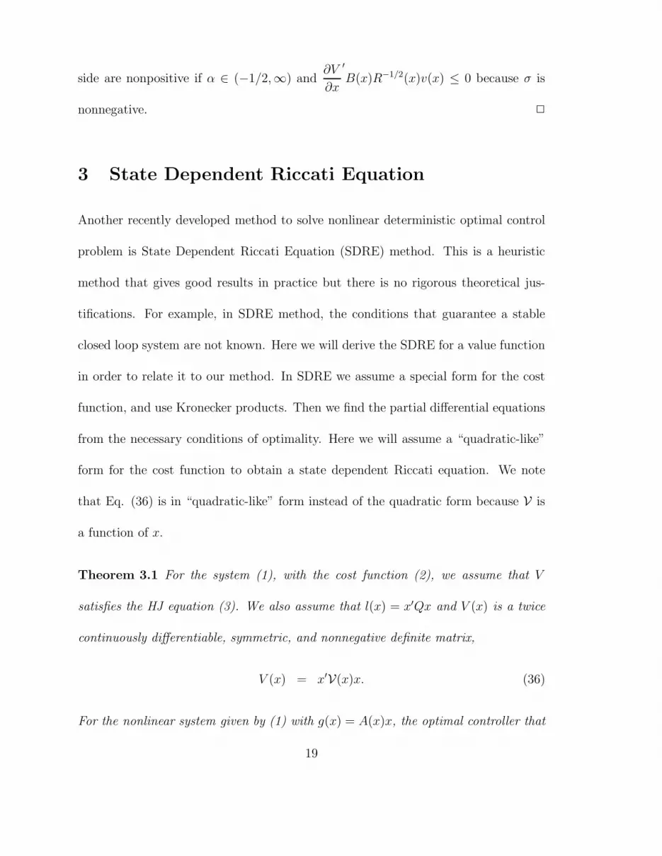
side are nonpositive if α ∈ (−1/2,∞) and∂V

∂x

′

B(x)R−1/2(x)v(x) ≤ 0 because σ is

nonnegative. 2

3 State Dependent Riccati Equation

Another recently developed method to solve nonlinear deterministic optimal control

problem is State Dependent Riccati Equation (SDRE) method. This is a heuristic

method that gives good results in practice but there is no rigorous theoretical jus-

tifications. For example, in SDRE method, the conditions that guarantee a stable

closed loop system are not known. Here we will derive the SDRE for a value function

in order to relate it to our method. In SDRE we assume a special form for the cost

function, and use Kronecker products. Then we find the partial differential equations

from the necessary conditions of optimality. Here we will assume a “quadratic-like”

form for the cost function to obtain a state dependent Riccati equation. We note

that Eq. (36) is in “quadratic-like” form instead of the quadratic form because V is

a function of x.

Theorem 3.1 For the system (1), with the cost function (2), we assume that V

satisfies the HJ equation (3). We also assume that l(x) = x′Qx and V (x) is a twice

continuously differentiable, symmetric, and nonnegative definite matrix,

V (x) = x′V(x)x. (36)

For the nonlinear system given by (1) with g(x) = A(x)x, the optimal controller that

19

minimizes the cost function (2) with l(x) = x′Q(x)x, is given by

k∗(x) = −1

2R−1(x)B′(x)

∂V (x)

∂x= −1

2R−1(x)B′

(

2V(x)x + (In ⊗ x′)∂V(x)

∂xx

)

. (37)

Provided that the following conditions are satisfied:

0 = A′(x)V(x) + V(x)A(x) + Q(x) − V(x)B(x)R−1(x)B′(x)V(x), (38)

√

R−1(x)B′(x)(In ⊗ x′)∂V(x)

∂x=√

R−1(x)B′(x)

[

∂V(x)

∂x⊗ x′

]

= 0, (39)

and

A(x)′(In ⊗ x′)∂V(x)

∂x= 0. (40)

Proof. Suppressing arguments for simplicity, we obtain the following HJ equation

using Eqs. (3) and (4)

0 = x′A′∂V

∂x− 1

4

(

∂V

∂x

)

′

BR−1B′∂V

∂x+ x′Qx. (41)

This is a necessary partial differential equation for the optimal control problem. Be-

cause V (x) is assumed to be symmetric and nonnegative definite matrix, we have

∂V

∂x= 2V(x)x + (In ⊗ x′)

∂V∂x

x, (42)

where ⊗ is the Kronecker product. Substitute the above equations into Equation (41)

to obtain

0 = x′Qx − x′VBR−1B′Vx

−[

(In ⊗ x′)∂V∂x

x

]

′

BR−1B′Vx − 1

4

[

(In ⊗ x′)∂V∂x

x

]

′

BR−1B′

[

(In ⊗ x′)∂V∂x

x

]

+x′A′2Vx + x′A′

[

(In ⊗ x′)∂V∂x

x

]

. (43)

20

Rewriting the above equation, we get

0 = x′

(

Q − VBR−1B′V + 2A′V)

x

+x′

[

−∂V∂x

′

(In ⊗ x′)′BR−1B′V − 1

4

∂V∂x

′

(In ⊗ x)BR−1B′(In ⊗ x′)∂V∂x

+ A′(In ⊗ x′)∂V∂x

]

x.

(44)

Thus, we obtain the three conditions in Eqs. (38), (39), and (40). And the optimal

controller is given by Eq. (37). 2

Remark 3.1 Note that for the special case when A(x) and B(x) are in the phase-

variable form of the state equation, the condition (39) is satisfied. Furthermore, both

conditions (39) and (40) are satisfied if∂V∂xi

= 0 for i = 1, · · · , n.

Example 3.1 Consider Example 2.2 in Section 2. Just rewriting the system equation

we have

x1

x2

=

−x21 1

0 1

x1

x2

+

0

1

k. (45)

Substituting the same Q and R matrices as in Example 2.2, and using Eq. (38) we

obtain,

V =

0 0

04 − 2

√7

3

.

And from Eq. (37) the optimal controller is determined to be

k∗ = −(

1 +

√7

2

)

x2.

This is the same controller as Section 2, Example 2.2. Because V is a constant in

this example, the state dependent Riccati equation (38) was the only requirement.

21

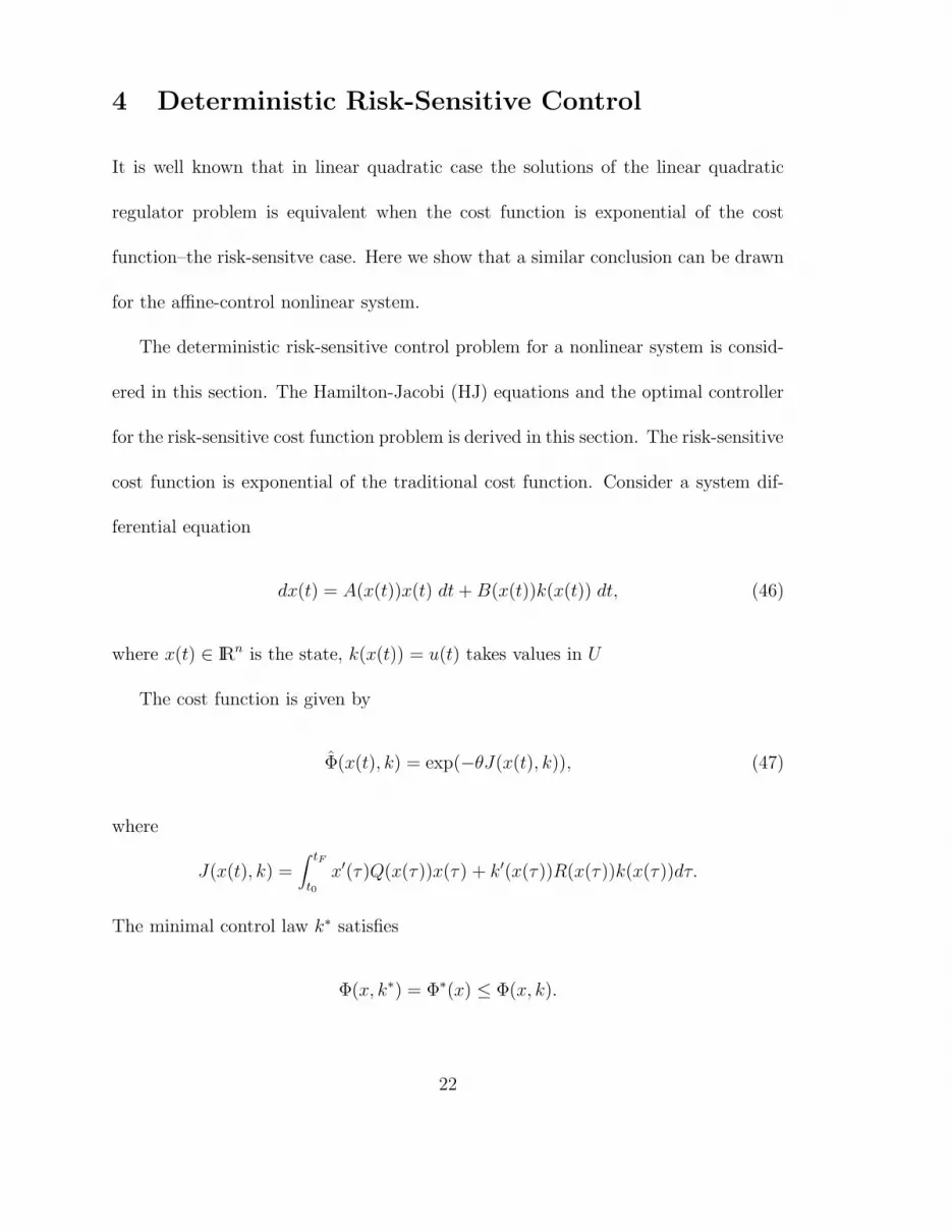
4 Deterministic Risk-Sensitive Control

It is well known that in linear quadratic case the solutions of the linear quadratic

regulator problem is equivalent when the cost function is exponential of the cost

function–the risk-sensitve case. Here we show that a similar conclusion can be drawn

for the affine-control nonlinear system.

The deterministic risk-sensitive control problem for a nonlinear system is consid-

ered in this section. The Hamilton-Jacobi (HJ) equations and the optimal controller

for the risk-sensitive cost function problem is derived in this section. The risk-sensitive

cost function is exponential of the traditional cost function. Consider a system dif-

ferential equation

dx(t) = A(x(t))x(t) dt + B(x(t))k(x(t)) dt, (46)

where x(t) ∈ IRn is the state, k(x(t)) = u(t) takes values in U

The cost function is given by

Φ(x(t), k) = exp(−θJ(x(t), k)), (47)

where

J(x(t), k) =∫ tF

t0x′(τ)Q(x(τ))x(τ) + k′(x(τ))R(x(τ))k(x(τ))dτ.

The minimal control law k∗ satisfies

Φ(x, k∗) = Φ∗(x) ≤ Φ(x, k).

22

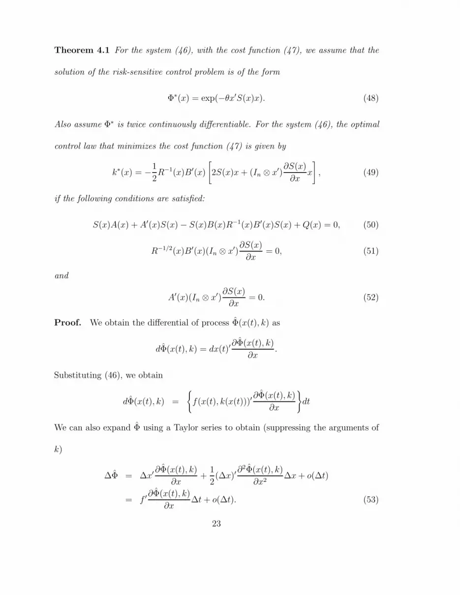
Theorem 4.1 For the system (46), with the cost function (47), we assume that the

solution of the risk-sensitive control problem is of the form

Φ∗(x) = exp(−θx′S(x)x). (48)

Also assume Φ∗ is twice continuously differentiable. For the system (46), the optimal

control law that minimizes the cost function (47) is given by

k∗(x) = −1

2R−1(x)B′(x)

[

2S(x)x + (In ⊗ x′)∂S(x)

∂xx

]

, (49)

if the following conditions are satisfied:

S(x)A(x) + A′(x)S(x) − S(x)B(x)R−1(x)B′(x)S(x) + Q(x) = 0, (50)

R−1/2(x)B′(x)(In ⊗ x′)∂S(x)

∂x= 0, (51)

and

A′(x)(In ⊗ x′)∂S(x)

∂x= 0. (52)

Proof. We obtain the differential of process Φ(x(t), k) as

dΦ(x(t), k) = dx(t)′∂Φ(x(t), k)

∂x.

Substituting (46), we obtain

dΦ(x(t), k) =

{

f(x(t), k(x(t)))′∂Φ(x(t), k)

∂x

}

dt

We can also expand Φ using a Taylor series to obtain (suppressing the arguments of

k)

∆Φ = ∆x′∂Φ(x(t), k)

∂x+

1

2(∆x)′

∂2Φ(x(t), k)

∂x2∆x + o(∆t)

= f ′∂Φ(x(t), k)

∂x∆t + o(∆t). (53)

23

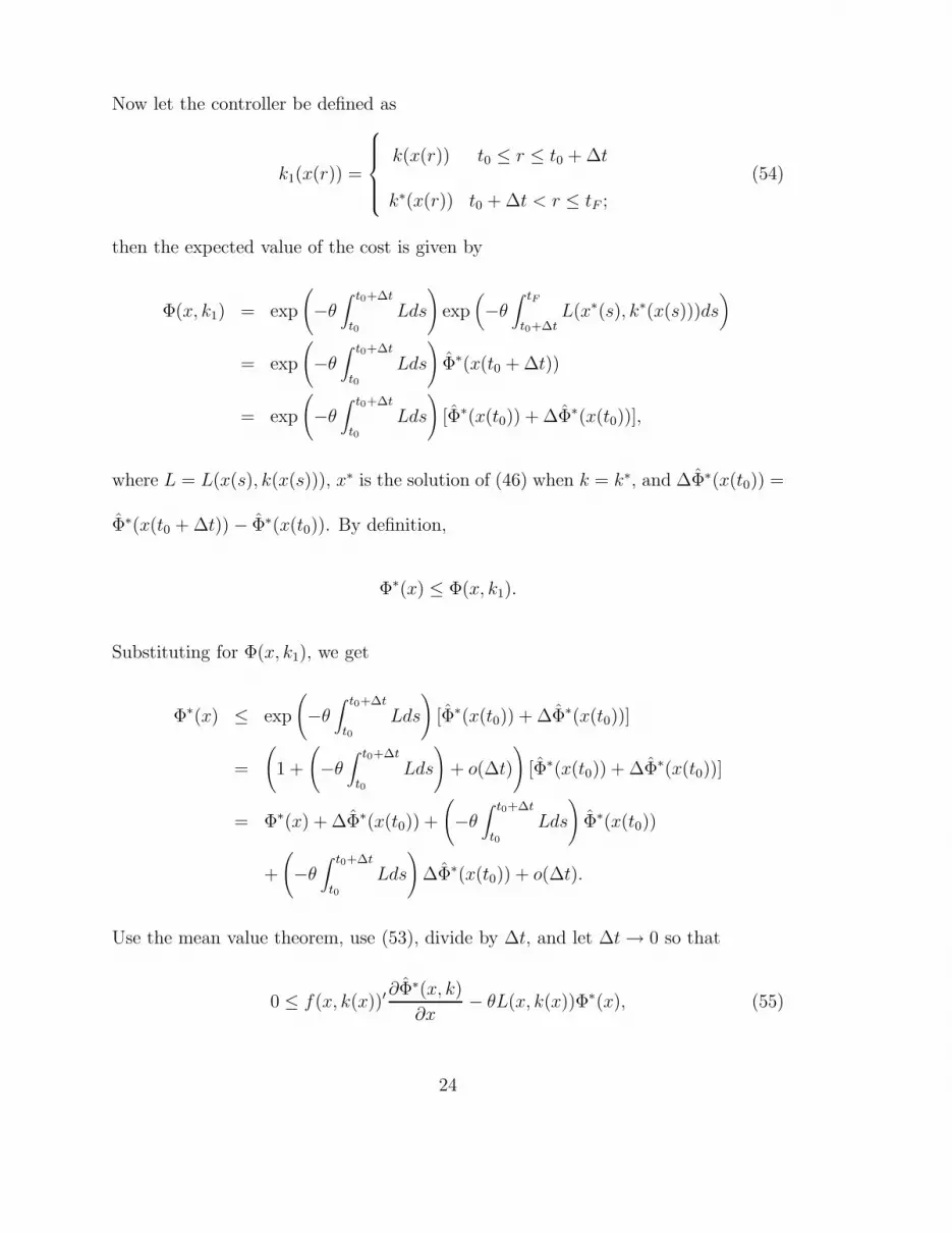
Now let the controller be defined as

k1(x(r)) =

k(x(r)) t0 ≤ r ≤ t0 + ∆t

k∗(x(r)) t0 + ∆t < r ≤ tF ;

(54)

then the expected value of the cost is given by

Φ(x, k1) = exp

(

−θ∫ t0+∆t

t0Lds

)

exp(

−θ∫ tF

t0+∆tL(x∗(s), k∗(x(s)))ds

)

= exp

(

−θ∫ t0+∆t

t0Lds

)

Φ∗(x(t0 + ∆t))

= exp

(

−θ∫ t0+∆t

t0Lds

)

[Φ∗(x(t0)) + ∆Φ∗(x(t0))],

where L = L(x(s), k(x(s))), x∗ is the solution of (46) when k = k∗, and ∆Φ∗(x(t0)) =

Φ∗(x(t0 + ∆t)) − Φ∗(x(t0)). By definition,

Φ∗(x) ≤ Φ(x, k1).

Substituting for Φ(x, k1), we get

Φ∗(x) ≤ exp

(

−θ∫ t0+∆t

t0Lds

)

[Φ∗(x(t0)) + ∆Φ∗(x(t0))]

=

(

1 +

(

−θ∫ t0+∆t

t0Lds

)

+ o(∆t)

)

[Φ∗(x(t0)) + ∆Φ∗(x(t0))]

= Φ∗(x) + ∆Φ∗(x(t0)) +

(

−θ∫ t0+∆t

t0Lds

)

Φ∗(x(t0))

+

(

−θ∫ t0+∆t

t0Lds

)

∆Φ∗(x(t0)) + o(∆t).

Use the mean value theorem, use (53), divide by ∆t, and let ∆t → 0 so that

0 ≤ f(x, k(x))′∂Φ∗(x, k)

∂x− θL(x, k(x))Φ∗(x), (55)

24

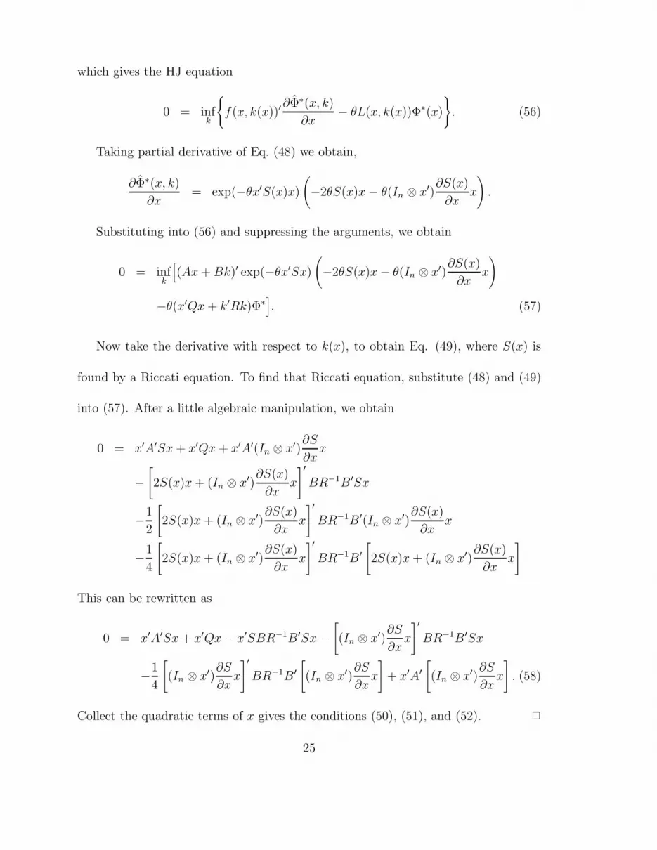
which gives the HJ equation

0 = infk

{

f(x, k(x))′∂Φ∗(x, k)

∂x− θL(x, k(x))Φ∗(x)

}

. (56)

Taking partial derivative of Eq. (48) we obtain,

∂Φ∗(x, k)

∂x= exp(−θx′S(x)x)

(

−2θS(x)x − θ(In ⊗ x′)∂S(x)

∂xx

)

.

Substituting into (56) and suppressing the arguments, we obtain

0 = infk

[

(Ax + Bk)′ exp(−θx′Sx)

(

−2θS(x)x − θ(In ⊗ x′)∂S(x)

∂xx

)

−θ(x′Qx + k′Rk)Φ∗

]

. (57)

Now take the derivative with respect to k(x), to obtain Eq. (49), where S(x) is

found by a Riccati equation. To find that Riccati equation, substitute (48) and (49)

into (57). After a little algebraic manipulation, we obtain

0 = x′A′Sx + x′Qx + x′A′(In ⊗ x′)∂S

∂xx

−[

2S(x)x + (In ⊗ x′)∂S(x)

∂xx

]

′

BR−1B′Sx

−1

2

[

2S(x)x + (In ⊗ x′)∂S(x)

∂xx

]

′

BR−1B′(In ⊗ x′)∂S(x)

∂xx

−1

4

[

2S(x)x + (In ⊗ x′)∂S(x)

∂xx

]

′

BR−1B′

[

2S(x)x + (In ⊗ x′)∂S(x)

∂xx

]

This can be rewritten as

0 = x′A′Sx + x′Qx − x′SBR−1B′Sx −[

(In ⊗ x′)∂S

∂xx

]

′

BR−1B′Sx

−1

4

[

(In ⊗ x′)∂S

∂xx

]

′

BR−1B′

[

(In ⊗ x′)∂S

∂xx

]

+ x′A′

[

(In ⊗ x′)∂S

∂xx

]

. (58)

Collect the quadratic terms of x gives the conditions (50), (51), and (52). 2

25

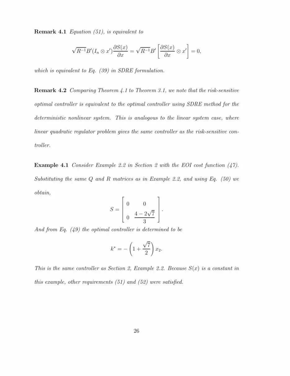
Remark 4.1 Equation (51), is equivalent to

√R−1B′(In ⊗ x′)

∂S(x)

∂x=

√R−1B′

[

∂S(x)

∂x⊗ x′

]

= 0,

which is equivalent to Eq. (39) in SDRE formulation.

Remark 4.2 Comparing Theorem 4.1 to Theorem 3.1, we note that the risk-sensitive

optimal controller is equivalent to the optimal controller using SDRE method for the

deterministic nonlinear system. This is analogous to the linear system case, where

linear quadratic regulator problem gives the same controller as the risk-sensitive con-

troller.

Example 4.1 Consider Example 2.2 in Section 2 with the EOI cost function (47).

Substituting the same Q and R matrices as in Example 2.2, and using Eq. (50) we

obtain,

S =

0 0

04 − 2

√7

3

.

And from Eq. (49) the optimal controller is determined to be

k∗ = −(

1 +

√7

2

)

x2.

This is the same controller as Section 2, Example 2.2. Because S(x) is a constant in

this example, other requirements (51) and (52) were satisfied.

26

5 Conclusions

For a affine-control nonlinear system with nonquadratic cost function, we pre-

sented a method to determine an optimal controller. We view the HJ equation as

an algebraic equation and solve for the gradient of the value function. Then this

gradient of the value function is used to obtain the optimal controller. Furthermore,

we investigated the robustness and stability properties of the optimal controller by

relating the value function to the control Lyapunov function. We showed that the

optimal controller is a stabilizing controller with good stability margins. Moreover,

we investigated two other nonlinear deterministic optimal control methods; state de-

pendent Riccati equation (SDRE) and risk-sensitive controls. First, we derived the

optimal controller through SDRE. Second, we derived an optimal controller when

the cost function is the exponential of the quadratic cost function which is the de-

terministic risk-sensitive control problem. We conclude that SDRE method gives an

equivalent optimal control as the risk-sensitive controller for a deterministic nonlinear

system. This will not be the case for stochastic systems. Simple examples illustrate

the developed optimal controller determination procedures.

6 Acknowledgments

This work is supported by the National Science Foundation grant, ECS-0554748.

27

References

[1] D. S. Bernstein, Matrix Mathematics, Princeton University Press, Princeton,New Jersey, 2005.

[2] C. I. Byrnes, A. Isidori, and J. C. Willems, “Passivity, Feedback Equivalence, andthe Global Stabilization of Minimum Phase Nonlinear Systems,” IEEE Transac-tions on Automatic Control, Vol. 36, No. 11, pp. 1228-1240, November 1991.

[3] J. R. Cloutier, C. N. D’Souza, and C. P. Mracek, “Nonlinear Regulation andNonlinear H∞ Control Via the State-Dependent Riccati Equation Technique:Part I, Theory; Prat II, Examples” Proceedings of the International Conferenceon Nonlinear Problems in Aviation and Aerospace, pp. 117–142, May 1996.

[4] J. W. Curtis and R. W. Beard, “Satisficing: A New Approach to ConstructiveNonlinear Control,” IEEE Transactions on Automatic Control, Vol. 49, No. 7,pp. 1090-1102, 2004.

[5] W. H. Fleming and R. W. Rishel, Deterministic and Stochastic Optimal Control,Springer-Verlag, New York, 1975.

[6] Freeman, R. A. and Kokotovic, P. V., “Optimal Nonlinear Controllers for Feed-back Linearizable Systems,” 1994 Workshop on Robust Control via VariableStructure and Lyapunov Techniques, Benevento, Italy, September 1994.

[7] Freeman, R. A. and Kokotovic, P. V., “Inverse Optimality in Robust Stabiliza-tion,” SIAM J. on Control and Optimization, Vol. 12, No. 4, pp. 1365-1391, July1996.

[8] S. Torkel Glad, “Robustness of Nonlinear State Feedback–A Survey,” Automat-ica, Vol. 23, No. 4, pp. 425-435, 1987.

[9] D. H. Jacobson, “Optimal Stochastic Linear Systems with Exponential Perfor-mance Criteria and Their Relationship to Deterministic Differential Games,”IEEE Transactions on Automatic Control, Volume AC-18, pp. 124–131, 1973.

[10] Miroslav Krstic, Ioannis Kanellakopoulos, and Petar Kokotovic, Nonlinear andAdaptive Control Design, John Wiley & Sons, Inc. 1995.

[11] P. Lancaster and M. Tismenetsky, The Theory of Matrices, Second Edition,Academic Press, 1985.

[12] R. W. Liu and J. Leake, “Inverse Lyapunov Problems,” Technical Report No. EE-6510, Department of Electrical Engineering, University of Notre Dame, August1965.

28

[13] Primbs, J. A. V. Nevistic, and J. C. Doyle, “A Receding Horizon Generalizationof Pointwise Min-Norm Controllers,” IEEE Transactions on Automatic Control,Vol. 45, No. 5, pp. 898-909, May 2000.

[14] Sain, M. K. Won, C.-H. Spencer Jr., B. F. and Liberty, S. R., “Cumulantsand Risk-Sensitive Control: A Cost Mean and Variance Theory with Appli-cation to Seismic Protection of Structures,” Advances in Dynamic Games andApplications, Annals of the International Society of Dynamic Games, Volume 5,pp. 427-459, Jerzy A Filar, Vladimir Gaitsgory, and Koichi Mizukami, Editors.Boston: Birkhauser, 2000.

[15] Sepulchre, R. Jankovic, M. Kokotovic, P. V. Constructive Nonlinear Control,Springer-Verlag, 1997.

[16] P. Whittle, “A Risk-Sensitive Maximum Principle: The Case of Imperfect StateObservation,” IEEE Transactions on Automatic Control, Vol. 36, No. 7, pp.793–801, July 1991.

[17] C.-. Won, “State-Feedback Optimal Controllers for Deterministic Nonlinear Sys-tems,” Proceedings American Control Conference, Portland, Oregon, pp. 858-863, June 8-10, 2005.

29

0 2 4 6 8 100

0.1

0.2

0.3

0.4

0.5

0.6

0.7

Time

Sta

te

Figure 1: The state, x, as a function of time, t.

30

0 1 2 3 4 50

1

2

3

4

5

6

x1

x 2

Figure 2: The phase portrait of Example 2.2 using an optimal controller

31

0 0.5 1 1.5 2 2.5 3 3.5 4 4.5 50

1

2

3

4

5

6

x1

x 2

Figure 3: The phase portrait of Example 2.2 using a min-norm controller

32

0 1 2 3 4 5−2

−1

0

1

2

3

4

5

6

x1

x 2

Figure 4: The phase portrait of Example 2.3 with nonquadratic cost using an optimalcontroller

33