International Journal of Pure and Applied Mathematics————————————————————————–Volume 31 No. 1 2006, 9-22

A PARAMETER SEARCH ALGORITHM BASED

ON OPTIMAL LINEAR CODES

Gregory M. Constantine1, John Bartels2, Marius Buliga3 §,Gilles Clermont4, Yoram Vodovotz5

1Department of MathematicsUniversity of Pittsburgh

Pittsburgh, PA 15260, USAe-mail: gmc@euler.math.pitt.edu

2Immunetrics, Inc.Pittsburgh, PA 15260, USA

3Department of MathematicsUniversity of Pittsburgh-Bradford

Bradford, PA 16701, USAe-mail: buliga@pitt.edu

4Department of Critical Care MedicineUniversity of Pittsburgh Medical Center

Pittsburgh, PA 15260, USA5 Department of Surgery

University of Pittsburgh Medical CenterPittsburgh, PA 15260, USA

Abstract: Modeling by way of dynamical systems often leads to systems ofordinary differential equations involving a large number of parameters, such asgrowth rates and initial conditions. A parameter search algorithm based onoptimal linear codes is developed having as aim the identification of differentregimes of behaviour of the model and its calibration to data.

AMS Subject Classification: 68R01, 37M05Key Words: optimization, differential equations, immune system, mathe-matical modeling

Received: June 7, 2006 c© 2006, Academic Publications Ltd.

§Correspondence author

10 G.M. Constantine, J. Bartels, M. Buliga, G. Clermont, Y. Vodovotz

1. Introduction

Acute systemic inflammation is triggered by stresses on a living organism suchas infection or trauma. This response involves a cascade of events mediated bya network of cells and molecules. The process localizes and identifies an insult,strives to eliminate offending agents, and initiates a repair process.

Complexities of the immune system are discussed in Bone [1], Mira et al [8]and Medzhitov [7]. It has been suggested that mathematical modeling mightprovide an effective tool to grapple with the complexity of the inflammatoryresponse to infection and trauma (Nathan [9], Buchman et al [2], Neugebaueret al [10]). Modeling is increasingly being used to address clinically relevantbiological complexity, in some cases leading to novel predictions (Kitano [5],Chow et al [3]). In silico simulations based on mathematical models have re-cently been shown to be useful at the therapeutic level; cf. Clermont et al [4].We embarked on an iterative process of model generation, verification and cal-ibration in animal models, and subsequent hypothesis generation. The model,described by a system of differential equations (see Chow et al [3] for explicitlists of the ordinary differential equations involved) aims to explain the reac-tion of the immune system in several scenarios, by engaging processes that takeplace at the molecular level. The focus of this paper is on the development of aglobal search strategy of the parameter space that aids in predicting regime be-haviour of the model as well as optimizing its fit to observed data. The generaloutline of the algorithm is presented in Section 2. Implementational issues arediscussed in Section 3, with comparisons with other known algorithms formingthe contents of Section 4. The regime classification and prediction, based on amultinomial logistic model, is described in the last section.

2. A Parameter Optimization Algorithm Based on Optimal Codes

The algorithm was developed out of the need to survey a high dimensionalparameter space in which varying one or two parameters at a time, while keepingthe others fixed, is simply not practical. It has at its core a (binary) codewith efficient covering properties of the high dimensional parameter space. Forexpository transparency we worked with Hamming (binary) codes, but othercodes over arbitrary finite fields with optimal covering properties may be used.The setting is that of a finite dimensional vector space V of dimension n overF2, the binary field, endowed with the usual inner product with values in F2.We specify the code as the orthogonal complement of the space generated by the

A PARAMETER SEARCH ALGORITHM BASED... 11

row vectors of a parity check matrix H of full row rank. The code is, therefore,

C = {x : Hx = 0}.

Let the dimension of C be k. Of equal interest are the cosets of the code. Acoset Cy is specified as follows:

Cy = {x : Hx = y},

where y is the “syndrome” vector defining the coset in question. Since C hasdimension k, the vector y is a column vector of dimension n− k. The set {Cy}represents the set of 2n−k cosets of C, as y runs over the set of all binary vectorsof dimension n − k. The reader is refered to MacWilliams and Sloane [6] formaterial on coding theory.

We write out some of the details for the Hamming code in 7 dimensions,assuming that we have seven parameters, defined by the parity check matrix

H =

1 0 1 0 1 0 10 1 1 0 0 1 10 0 0 1 1 1 1

.

This matrix H yields a code of dimension 4, consisting of 16 binary vectors.

We shall make use of a binary code C in the following way. The responsefunction f of n (usually real) parameters x1, . . . , xn is to be investigated overa product space B =

∏ni=1[ai, bi], with ai ≤ xi ≤ bi; 1 ≤ i ≤ n. For illustrative

purposes we assume that the usually vector-valued response function is a scalarfunction. This function is in practice obtained by integrating the ODE systemnumerically (which we call the model) and assigning a measure of discrepancybetween the model and the data. To describe how the algorithm works weassume that we want to numerically find the minimum of f over B. Take avector x = (x1, . . . , xn) ∈ B. Code x as a binary vector by placing a 0 incoordinate position i if xi ∈ [ai,

ai+bi

2 ] and a 1 otherwise; write x̄ for the codedx.

By either a deliberate or a random process select a point xi0 ∈ [ai,ai+bi

2 ] =

Bi0 and a point xi1 ∈ (ai+bi

2 , bi] = Bi1; 1 ≤ i ≤ n. A point (x1j1 , . . . , xnjn), withjm being either 0 or 1, belongs to the “cell”

∏ni=1 Biji

. Consider now the set ofcoded points of B,

{(x̄1j , . . . , x̄nj) : j = 0, 1}.

This process defines 2n binary vectors which we now view as the elements ofan n−dimensional vector space V over the field with two elements F2. Indeed,

12 G.M. Constantine, J. Bartels, M. Buliga, G. Clermont, Y. Vodovotz

with the points xij fixed, the correspondence

(x1j1 , . . . , xnjn) ↔ (x̄1j1, . . . , x̄njn),

with jm = 0 or 1, is a bijection by way of which we shall identify the selectedpoints of B, which we denote by V (B), with elements of V. In particular, anysubset S of points of V identifies through this bijection a corresponding set ofpoints in B, which we write as S(B). This is the case with the set of vectors ina linear code C of V as well. If C is a linear code of dimension k, the subsetC(B) consists of 2k points in B. By abuse of language, we may on occasionrefer to C(B) as the points of the code C.

If the objective is to minimize function f over B, the algorithm first identifiesthe cells Bij associated with the code C. Within each cell Bij the algorithmreplicates itself, that is, it treats cell Bij as a new space B. It selects points inBij in accordance to (a code equivalent to) C (two codes are called equivalent ifone is obtained from the other upon a permutation of coordinates). We evaluatethe function f at all points selected in Bij , for all cells Bij. This allows us toidentify a subset L of cells that yield the smallest values of f. If the minimumobtained so far is satisfactory, we stop. Else we iterate the procedure withineach of the cells in L. This allows evaluation of the function f on a finer localmesh (at a deeper level of iteration). The nested level may be repeated anynumber of times. We stop when the minimum reached on f is sufficiently low.The list L keeps tabs of the addresses of the cells of interest at the various levelsof iteration. All this happens only for cells associated with the code C. We canthus select from list L a point xC (found in some cell of code C) such thatf(xC) is the smallest value of f found so far. Produce the list of differences

L = {f(x)−f(xC )||x−xC || : x ∈ C(B)} and select x0 ∈ C(B) such that f(x0)−f(xC )

||x0−xC || is

maximal (in general x in the list L actually runs over the set of cosets selectedso far). Along the line xC − t(x0−xC) find a smallest positive value t0 of t suchthat xC − t0(x0 − xC) is in a cell of V (B) not examined thus far. The codedversion of xC − t0(x0 −xC) = y defines a vector in V not previously considered,and hence identifies a new coset Cy = y + C of C. Before moving to the nextcoset a local analysis of the best cells found so far is performed as described indetail in the implementational section.

The coset Cy thus identified has the same optimal covering properties of V

as does C. The process followed for code C is now repeated for the coset Cy.

After examining m ≤ n−k cosets of C, call them {Cy1, . . . , Cym} (let y1 = 0, so

Cy1= C), we obtain m points P = {xCyi

: 1 ≤ i ≤ m} from the correspondingm lists. The point in P at which f attains a minimum is the point the algorithmgives as solution to the optimization problem. The algorithm thus combines

A PARAMETER SEARCH ALGORITHM BASED... 13

local gradient properties with global reach throughout the region B by way ofthe cosets of the code C.

3. Implementational Issues

This recursive process of subdivision and evaluation provides a general frame-work for our search algorithm. In order to actually implement this as a proce-dure, we must make several decisions about the details of our search process.Below we discuss the major considerations that must be addressed, and presentour strategies for dealing with them.

3.1. Search Procedure

The search algorithm proceeds in a manner similar to A* search; that is, we gen-erate candidate subregions of the space to be searched, compute an estimatedquality score for each candidate, and build a ranked list of these candidates. Oneach iteration of the algorithm, we remove the most promising region from thefront of the list, evaluate sample points within that region to update our qualityestimate, re-insert the updated region into the list, and possibly add to the listnew candidate regions discovered during evaluation. As discussed later, someadditional work may be done to bound the list growth within finite memorylimitations. The following discussion assumes the existence of a customizableranking function R(c), which computes a measure of the quality of a given cellc in the coded space V . While the choice of R(c) is crucial to succesful use ofthe algorithm, the search procedure itself is independent of how R(c) is defined.Our discussion casts the search as a minimization problem and thus assumesthat lower values of the objective function f(x) and the ranking function R(c)are preferred, though this could be inverted for maximization problems. Im-mediately below we describe the details of the search procedure in terms of anabstract R(c), while discussion of the design considerations for a concrete R(c)are continued later.

We require initial bounds for each parameter Pi, of the form Pi ∈ [Li,Hi].These bounds completely specify the n-dimensional search space B, and thusdefine our initial search cell c0. We create the empty ranked-cell list L, andinsert a record for c0 into this list. We also define Sb to be the best solutionever seen, and initially set it to null. The routine then selects the most promisingcell c from L, such that R(c) ≤ R(c′) for all c′ in L. The next step is to performan evaluation of c, which requires a design decision on how to apply the code

14 G.M. Constantine, J. Bartels, M. Buliga, G. Clermont, Y. Vodovotz

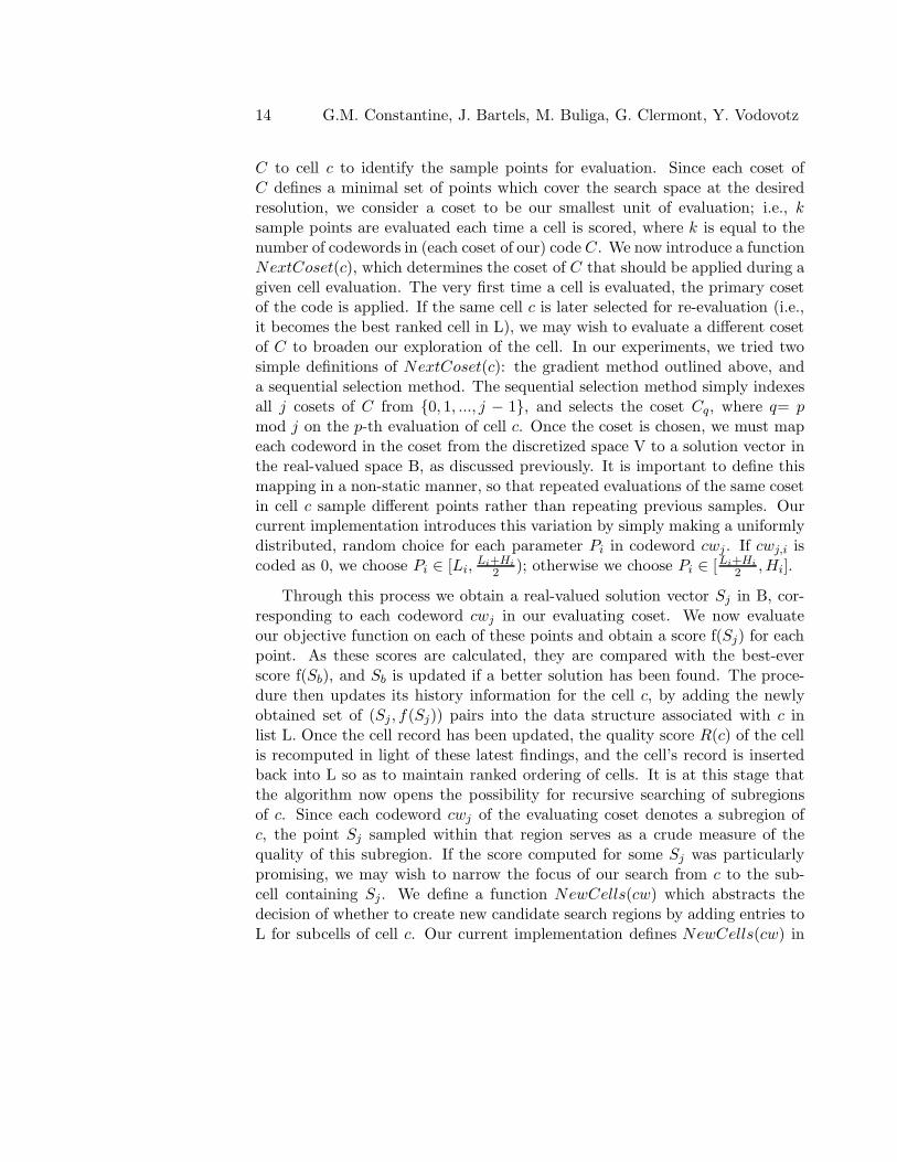
C to cell c to identify the sample points for evaluation. Since each coset ofC defines a minimal set of points which cover the search space at the desiredresolution, we consider a coset to be our smallest unit of evaluation; i.e., k

sample points are evaluated each time a cell is scored, where k is equal to thenumber of codewords in (each coset of our) code C. We now introduce a functionNextCoset(c), which determines the coset of C that should be applied during agiven cell evaluation. The very first time a cell is evaluated, the primary cosetof the code is applied. If the same cell c is later selected for re-evaluation (i.e.,it becomes the best ranked cell in L), we may wish to evaluate a different cosetof C to broaden our exploration of the cell. In our experiments, we tried twosimple definitions of NextCoset(c): the gradient method outlined above, anda sequential selection method. The sequential selection method simply indexesall j cosets of C from {0, 1, ..., j − 1}, and selects the coset Cq, where q= p

mod j on the p-th evaluation of cell c. Once the coset is chosen, we must mapeach codeword in the coset from the discretized space V to a solution vector inthe real-valued space B, as discussed previously. It is important to define thismapping in a non-static manner, so that repeated evaluations of the same cosetin cell c sample different points rather than repeating previous samples. Ourcurrent implementation introduces this variation by simply making a uniformlydistributed, random choice for each parameter Pi in codeword cwj . If cwj,i iscoded as 0, we choose Pi ∈ [Li,

Li+Hi

2 ); otherwise we choose Pi ∈ [Li+Hi

2 ,Hi].

Through this process we obtain a real-valued solution vector Sj in B, cor-responding to each codeword cwj in our evaluating coset. We now evaluateour objective function on each of these points and obtain a score f(Sj) for eachpoint. As these scores are calculated, they are compared with the best-everscore f(Sb), and Sb is updated if a better solution has been found. The proce-dure then updates its history information for the cell c, by adding the newlyobtained set of (Sj , f(Sj)) pairs into the data structure associated with c inlist L. Once the cell record has been updated, the quality score R(c) of the cellis recomputed in light of these latest findings, and the cell’s record is insertedback into L so as to maintain ranked ordering of cells. It is at this stage thatthe algorithm now opens the possibility for recursive searching of subregionsof c. Since each codeword cwj of the evaluating coset denotes a subregion ofc, the point Sj sampled within that region serves as a crude measure of thequality of this subregion. If the score computed for some Sj was particularlypromising, we may wish to narrow the focus of our search from c to the sub-cell containing Sj. We define a function NewCells(cw) which abstracts thedecision of whether to create new candidate search regions by adding entries toL for subcells of cell c. Our current implementation defines NewCells(cw) in

A PARAMETER SEARCH ALGORITHM BASED... 15

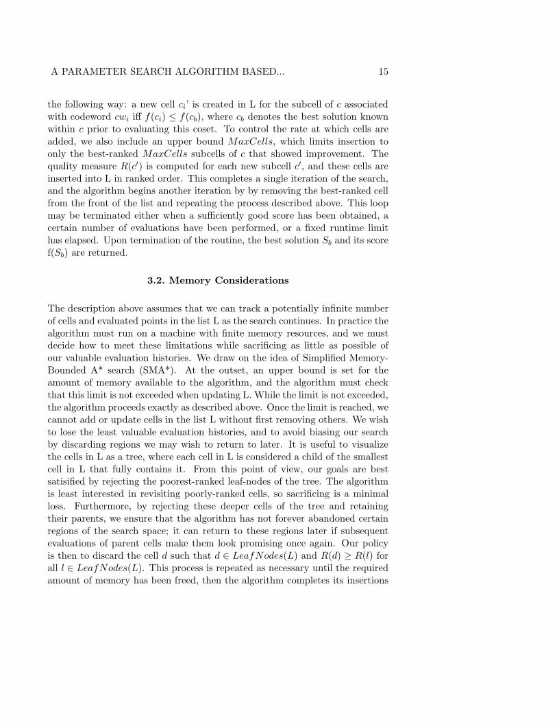
the following way: a new cell ci’ is created in L for the subcell of c associatedwith codeword cwi iff f(ci) ≤ f(cb), where cb denotes the best solution knownwithin c prior to evaluating this coset. To control the rate at which cells areadded, we also include an upper bound MaxCells, which limits insertion toonly the best-ranked MaxCells subcells of c that showed improvement. Thequality measure R(c′) is computed for each new subcell c′, and these cells areinserted into L in ranked order. This completes a single iteration of the search,and the algorithm begins another iteration by by removing the best-ranked cellfrom the front of the list and repeating the process described above. This loopmay be terminated either when a sufficiently good score has been obtained, acertain number of evaluations have been performed, or a fixed runtime limithas elapsed. Upon termination of the routine, the best solution Sb and its scoref(Sb) are returned.

3.2. Memory Considerations

The description above assumes that we can track a potentially infinite numberof cells and evaluated points in the list L as the search continues. In practice thealgorithm must run on a machine with finite memory resources, and we mustdecide how to meet these limitations while sacrificing as little as possible ofour valuable evaluation histories. We draw on the idea of Simplified Memory-Bounded A* search (SMA*). At the outset, an upper bound is set for theamount of memory available to the algorithm, and the algorithm must checkthat this limit is not exceeded when updating L. While the limit is not exceeded,the algorithm proceeds exactly as described above. Once the limit is reached, wecannot add or update cells in the list L without first removing others. We wishto lose the least valuable evaluation histories, and to avoid biasing our searchby discarding regions we may wish to return to later. It is useful to visualizethe cells in L as a tree, where each cell in L is considered a child of the smallestcell in L that fully contains it. From this point of view, our goals are bestsatisified by rejecting the poorest-ranked leaf-nodes of the tree. The algorithmis least interested in revisiting poorly-ranked cells, so sacrificing is a minimalloss. Furthermore, by rejecting these deeper cells of the tree and retainingtheir parents, we ensure that the algorithm has not forever abandoned certainregions of the search space; it can return to these regions later if subsequentevaluations of parent cells make them look promising once again. Our policyis then to discard the cell d such that d ∈ LeafNodes(L) and R(d) ≥ R(l) forall l ∈ LeafNodes(L). This process is repeated as necessary until the requiredamount of memory has been freed, then the algorithm completes its insertions

16 G.M. Constantine, J. Bartels, M. Buliga, G. Clermont, Y. Vodovotz

and resumes.

3.3. Design of Ranking Functions

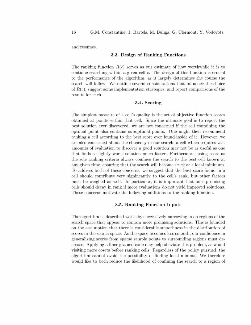
The ranking function R(c) serves as our estimate of how worthwhile it is tocontinue searching within a given cell c. The design of this function is crucialto the performance of the algorithm, as it largely determines the course thesearch will follow. We outline several considerations that influence the choiceof R(c), suggest some implementation strategies, and report comparisons of theresults for each.

3.4. Scoring

The simplest measure of a cell’s quality is the set of objective function scoresobtained at points within that cell. Since the ultimate goal is to report thebest solution ever discovered, we are not concerned if the cell containing theoptimal point also contains suboptimal points. One might then recommendranking a cell according to the best score ever found inside of it. However, weare also concerned about the efficiency of our search; a cell which requires vastamounts of evaluation to discover a good solution may not be as useful as onethat finds a slightly worse solution much faster. Furthermore, using score asthe sole ranking criteria always confines the search to the best cell known atany given time, ensuring that the search will become stuck at a local minimum.To address both of these concerns, we suggest that the best score found in acell should contribute very significantly to the cell’s rank, but other factorsmust be weighed as well. In particular, it is important that once-promisingcells should decay in rank if more evaluations do not yield improved solutions.These concerns motivate the following additions to the ranking function.

3.5. Ranking Function Inputs

The algorithm as described works by successively narrowing in on regions of thesearch space that appear to contain more promising solutions. This is foundedon the assumption that there is considerable smoothness in the distribution ofscores in the search space. As the space becomes less smooth, our confidence ingeneralizing scores from sparse sample points to surrounding regions must de-crease. Applying a finer-grained code may help alleviate this problem, as wouldvisiting more cosets before ranking cells. Regardless of the policy pursued, thealgorithm cannot avoid the possibility of finding local minima. We thereforewould like to both reduce the likelihood of confining the search to a region of

A PARAMETER SEARCH ALGORITHM BASED... 17

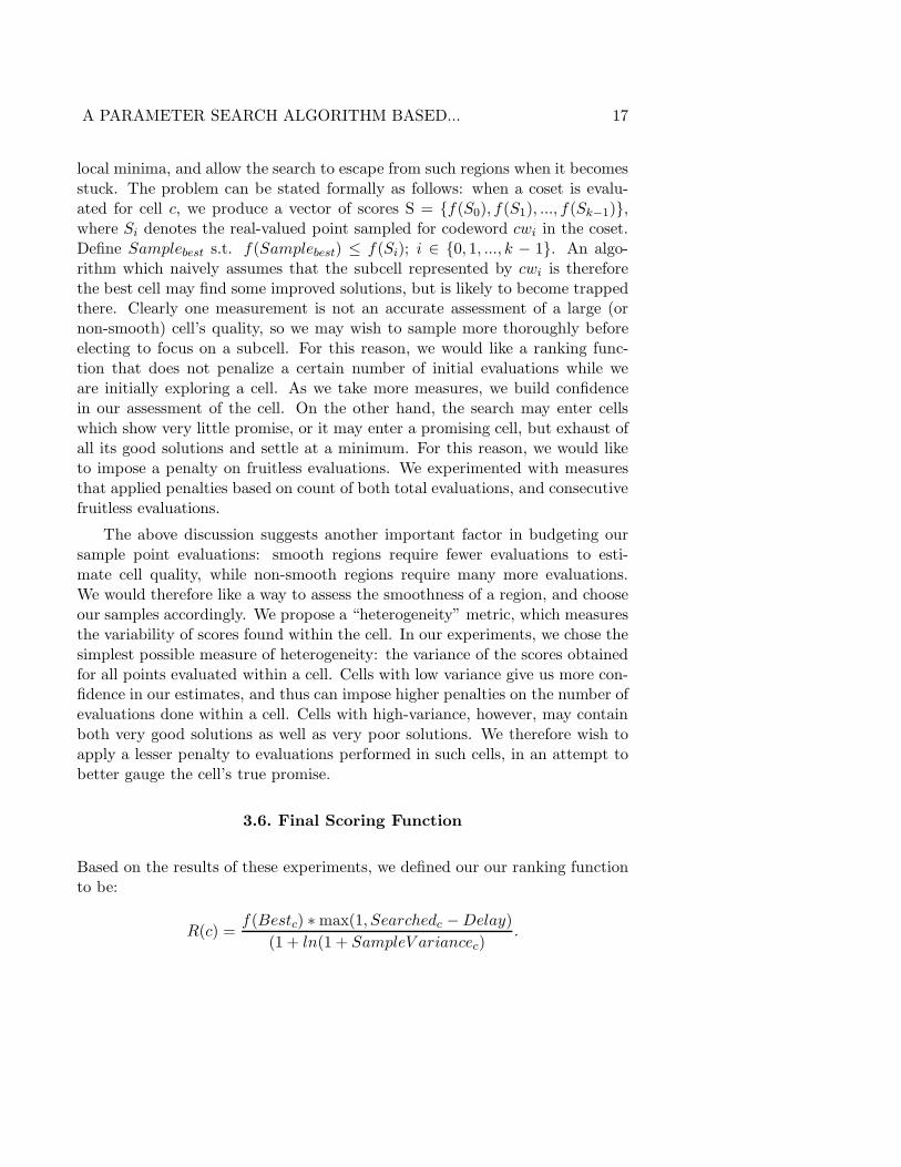
local minima, and allow the search to escape from such regions when it becomesstuck. The problem can be stated formally as follows: when a coset is evalu-ated for cell c, we produce a vector of scores S = {f(S0), f(S1), ..., f(Sk−1)},where Si denotes the real-valued point sampled for codeword cwi in the coset.Define Samplebest s.t. f(Samplebest) ≤ f(Si); i ∈ {0, 1, ..., k − 1}. An algo-rithm which naively assumes that the subcell represented by cwi is thereforethe best cell may find some improved solutions, but is likely to become trappedthere. Clearly one measurement is not an accurate assessment of a large (ornon-smooth) cell’s quality, so we may wish to sample more thoroughly beforeelecting to focus on a subcell. For this reason, we would like a ranking func-tion that does not penalize a certain number of initial evaluations while weare initially exploring a cell. As we take more measures, we build confidencein our assessment of the cell. On the other hand, the search may enter cellswhich show very little promise, or it may enter a promising cell, but exhaust ofall its good solutions and settle at a minimum. For this reason, we would liketo impose a penalty on fruitless evaluations. We experimented with measuresthat applied penalties based on count of both total evaluations, and consecutivefruitless evaluations.

The above discussion suggests another important factor in budgeting oursample point evaluations: smooth regions require fewer evaluations to esti-mate cell quality, while non-smooth regions require many more evaluations.We would therefore like a way to assess the smoothness of a region, and chooseour samples accordingly. We propose a “heterogeneity” metric, which measuresthe variability of scores found within the cell. In our experiments, we chose thesimplest possible measure of heterogeneity: the variance of the scores obtainedfor all points evaluated within a cell. Cells with low variance give us more con-fidence in our estimates, and thus can impose higher penalties on the number ofevaluations done within a cell. Cells with high-variance, however, may containboth very good solutions as well as very poor solutions. We therefore wish toapply a lesser penalty to evaluations performed in such cells, in an attempt tobetter gauge the cell’s true promise.

3.6. Final Scoring Function

Based on the results of these experiments, we defined our our ranking functionto be:

R(c) =f(Bestc) ∗ max(1, Searchedc − Delay)

(1 + ln(1 + SampleV ariancec).

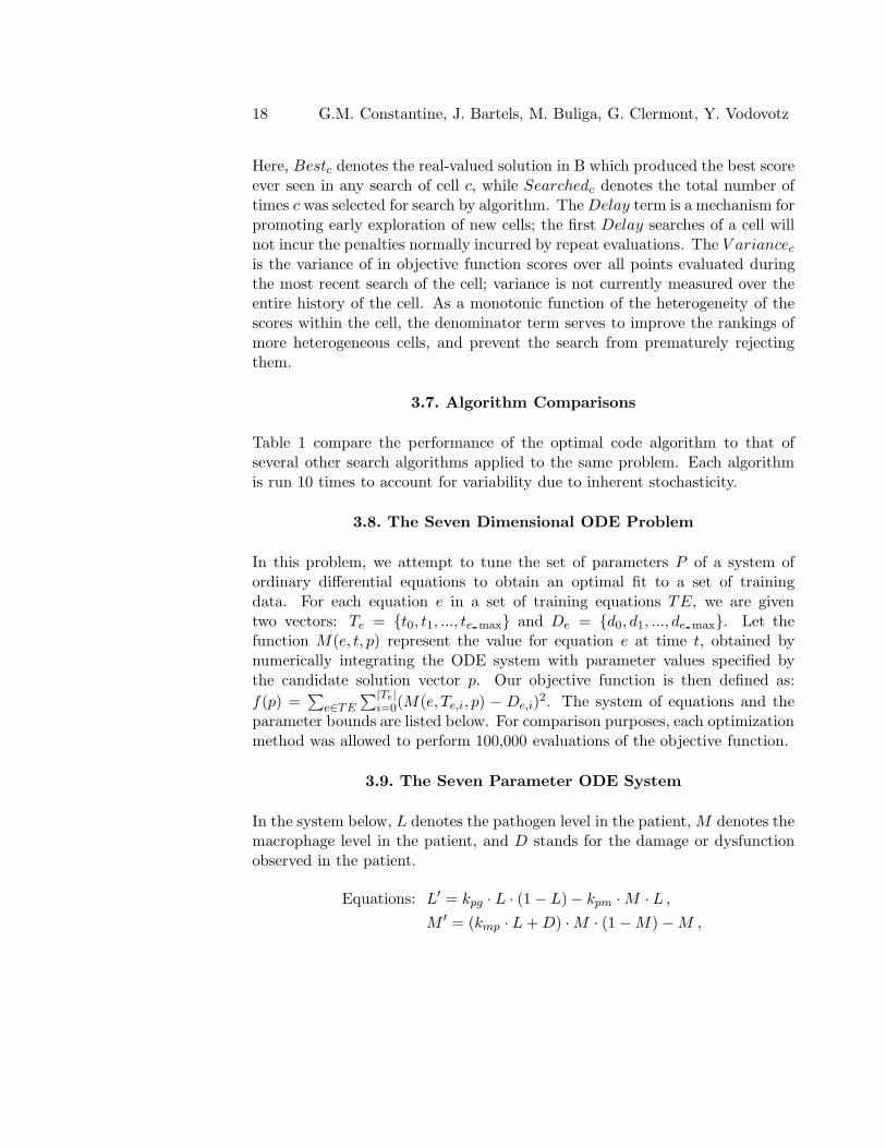
18 G.M. Constantine, J. Bartels, M. Buliga, G. Clermont, Y. Vodovotz

Here, Bestc denotes the real-valued solution in B which produced the best scoreever seen in any search of cell c, while Searchedc denotes the total number oftimes c was selected for search by algorithm. The Delay term is a mechanism forpromoting early exploration of new cells; the first Delay searches of a cell willnot incur the penalties normally incurred by repeat evaluations. The V ariancec

is the variance of in objective function scores over all points evaluated duringthe most recent search of the cell; variance is not currently measured over theentire history of the cell. As a monotonic function of the heterogeneity of thescores within the cell, the denominator term serves to improve the rankings ofmore heterogeneous cells, and prevent the search from prematurely rejectingthem.

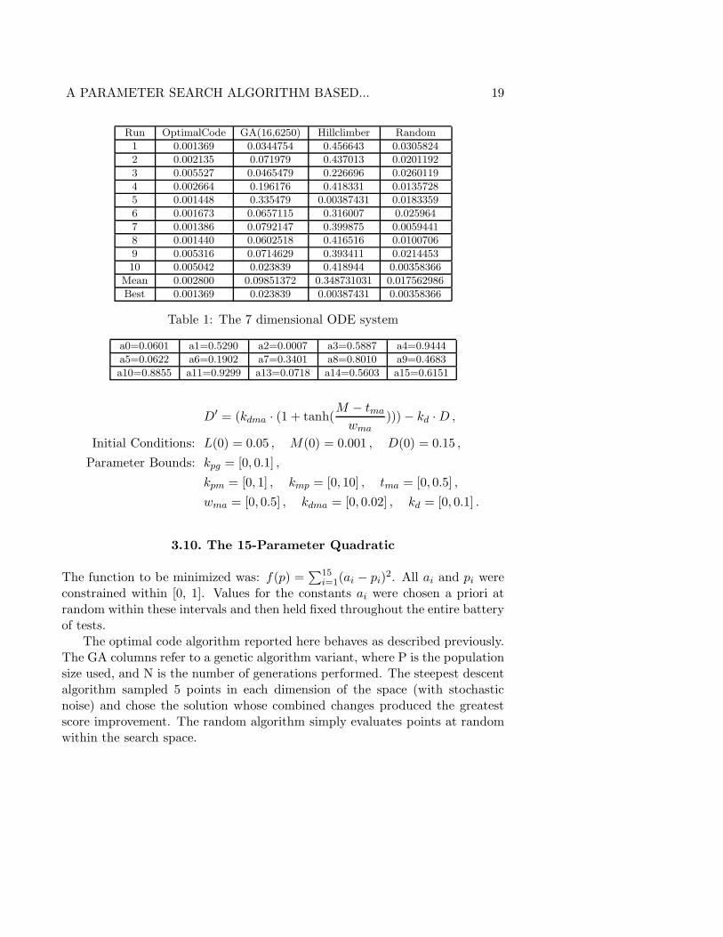
3.7. Algorithm Comparisons

Table 1 compare the performance of the optimal code algorithm to that ofseveral other search algorithms applied to the same problem. Each algorithmis run 10 times to account for variability due to inherent stochasticity.

3.8. The Seven Dimensional ODE Problem

In this problem, we attempt to tune the set of parameters P of a system ofordinary differential equations to obtain an optimal fit to a set of trainingdata. For each equation e in a set of training equations TE, we are giventwo vectors: Te = {t0, t1, ..., te max} and De = {d0, d1, ..., de max}. Let thefunction M(e, t, p) represent the value for equation e at time t, obtained bynumerically integrating the ODE system with parameter values specified bythe candidate solution vector p. Our objective function is then defined as:

f(p) =∑

e∈TE

∑|Te|i=0(M(e, Te,i, p) − De,i)

2. The system of equations and theparameter bounds are listed below. For comparison purposes, each optimizationmethod was allowed to perform 100,000 evaluations of the objective function.

3.9. The Seven Parameter ODE System

In the system below, L denotes the pathogen level in the patient, M denotes themacrophage level in the patient, and D stands for the damage or dysfunctionobserved in the patient.

Equations: L′ = kpg · L · (1 − L) − kpm · M · L ,

M ′ = (kmp · L + D) · M · (1 − M) − M ,

A PARAMETER SEARCH ALGORITHM BASED... 19

Run OptimalCode GA(16,6250) Hillclimber Random

1 0.001369 0.0344754 0.456643 0.0305824

2 0.002135 0.071979 0.437013 0.0201192

3 0.005527 0.0465479 0.226696 0.0260119

4 0.002664 0.196176 0.418331 0.0135728

5 0.001448 0.335479 0.00387431 0.0183359

6 0.001673 0.0657115 0.316007 0.025964

7 0.001386 0.0792147 0.399875 0.0059441

8 0.001440 0.0602518 0.416516 0.0100706

9 0.005316 0.0714629 0.393411 0.0214453

10 0.005042 0.023839 0.418944 0.00358366

Mean 0.002800 0.09851372 0.348731031 0.017562986

Best 0.001369 0.023839 0.00387431 0.00358366

Table 1: The 7 dimensional ODE system

a0=0.0601 a1=0.5290 a2=0.0007 a3=0.5887 a4=0.9444

a5=0.0622 a6=0.1902 a7=0.3401 a8=0.8010 a9=0.4683

a10=0.8855 a11=0.9299 a13=0.0718 a14=0.5603 a15=0.6151

D′ = (kdma · (1 + tanh(M − tma

wma

))) − kd · D ,

Initial Conditions: L(0) = 0.05 , M(0) = 0.001 , D(0) = 0.15 ,

Parameter Bounds: kpg = [0, 0.1] ,

kpm = [0, 1] , kmp = [0, 10] , tma = [0, 0.5] ,

wma = [0, 0.5] , kdma = [0, 0.02] , kd = [0, 0.1] .

3.10. The 15-Parameter Quadratic

The function to be minimized was: f(p) =∑15

i=1(ai − pi)2. All ai and pi were

constrained within [0, 1]. Values for the constants ai were chosen a priori atrandom within these intervals and then held fixed throughout the entire batteryof tests.

The optimal code algorithm reported here behaves as described previously.The GA columns refer to a genetic algorithm variant, where P is the populationsize used, and N is the number of generations performed. The steepest descentalgorithm sampled 5 points in each dimension of the space (with stochasticnoise) and chose the solution whose combined changes produced the greatestscore improvement. The random algorithm simply evaluates points at randomwithin the search space.

20 G.M. Constantine, J. Bartels, M. Buliga, G. Clermont, Y. Vodovotz

Run OptimalCode GA(2048,44) Hillclimber Random

1 0.0832361 1.83559 1.97709e-05 68.379

2 0.217762 1.68968 2.22564e-05 60.54

3 0.0772086 1.68611 1.3165e-05 68.1213

4 0.220271 2.62141 1.1364e-05 66.9669

5 0.540058 1.72501 9.60819e-06 69.3401

6 0.229307 2.22178 1.08077e-05 79.7582

7 0.169243 1.23769 3.66222e-05 55.4995

8 0.0960766 3.02225 1.51147e-05 74.71

9 0.299546 2.87475 5.29135e-06 94.2987

10 0.320636 4.24115 2.10776e-05 72.1723

Mean 0.22533443 2.315542 1.6507804e-05 70.9786

Best 0.0772086 1.23769 5.29135e-06 55.4995

Table 2: The 15-dimensional quadratic

4. Classifying Parameter Sets Yielding Different Regimes

Though minimizing an objective function occurs any time one fits a modelto data, one of our main objectives is to predict the correct regime for a givenvector of parameters. The first step is to identify originally a set of regimes thatthe system of ODE’s could produce; see also Neugebauer [10]. While severalpotential regimes may be suspected to exist a priori, not all possible regimes willusually be known. However, each time we evaluate the model at a parameterset (i.e., numerically integrate it) we either classify the resulting function in oneof the known regimes or decide to create a new regime. We can thus eventuallyexpand the set of regimes as the computer simulation progresses. Comparison ofregimes involves defining a measure that compares two regimes and computesa distance between them. We decided to use a measure that matches only“qualitatively defining features” of the functions in questions, such as notablepeaks, tail behaviour, or other qualitatively relevant traits. We shall then saythat two functions are in the same regime if they have qualitatively similarfeatures; else they represent different regimes (this measure is quite differentfor the more usual least squares metric, but it addresses better the qualitativefeatures we seek in the model).

We now describe how we can use the algorithm in the previous section inconjunction with a multinomial logistic distribution to classify any point in theparameter space. The outcomes of the logistic distribution are the r distinctregimes. We now start the algorithm. At each parameter point selected, byintegrating the ODE system, we obtain the response function. We computedistances to each of the r regimes and classify that parameter point in one of

A PARAMETER SEARCH ALGORITHM BASED... 21

them. The code ensures that the parameter space is optimally covered each timewe select a new coset of parameter points. After a sufficiently large number ofiterations we may notice points in the parameter space, where bifurcations seemto occur. In the neighborhood of such points (should they prove of investigativeinterest) we can locally replicate the search just described. We refer to Seydel[11] for detailed information on issues related to bifurcation.

To classify an arbitrary parameter point θ we use the multinomial logisticas follows: think of the points in the parameter space that we evaluated andclassified as data for the logistic model. Using maximum likelihood estimation,in the usual way, estimate from this data the coefficients in the logistic func-tion. Use the multinomial logistic model thus created to predict that θ yieldsa response in regime i with probability pi (with the pi summing to 1). Theprobabilities pi are estimated from the predictive equations generated by themultinomial logistic model. As is commonly done, we now classify θ in the classcorresponding to regime j, where j is defined by pj = max1≤i≤r pi.

Acknowledgments

The work is funded under the NIH grant GM67240.

References

[1] R.C. Bone, Immunologic dissonance: a continuing evolution in our under-standing of the systemic inflammatory response syndrome (SIRS) and themultiple organ dysfunction syndrome (MODS), Ann. Intern. Med., 125

(1996), 680-687.

[2] T.G. Buchman, J.P. Cobb, A.S. Lapedes, et al, Complex systems analysis:a tool for shock research, Shock, 16 (2001), 248-251.

[3] C.C. Chow, et al, Quantitative dynamics of the acute inflammatory re-sponse in shock states, American Journal of Physiology (2004), To Appear.

[4] G. Clermont, et al, In silico modeling of clinical trials: a method comingof age, Critical Care Medicine (2004), To Appear.

[5] H. Kitano, Systems biology: a brief overview, Science, 295 (2002), 1662-1664.

22 G.M. Constantine, J. Bartels, M. Buliga, G. Clermont, Y. Vodovotz

[6] F.J. MacWilliams, N.J.A. Sloane, The Theory of Error Correcting Codes,North Holland, Amsterdam (1978).

[7] R. Medzhitov, C.J. Janeway, Innate immunity, N. Engl. J. Med., 343

(2000), 338-344.

[8] J.P. Mira, A. Cariou, F. Grall, et al, Association of TNF2, a TNF-a pro-moter polymorphism, with septic shock susceptibility and mortality. Amulticenter study, JAMA, 282 (1999), 561-568.

[9] C. Nathan, Points of control in inflammation, Nature, 420 (2002), 846-852.

[10] E.A. Neugebauer, C. Willy, S. Sauerland, Complexity and non-linearity inshock research: reductionism or synthesis?, Shock, 16 (2001), 252-258.

[11] R. Seydel, Practical Bifurcation and Stability Analysis: From Equilibrium

to Chaos, Second Edition, Springer Verlag, New York (1994).