Optimal design for prediction using local linear

regression and the DSI-criterion

Verity A. Fisher, David C. Woods and Susan M. LewisUniversity of Southampton, Southampton, UK

{V.Fisher,D.Woods,S.M.Lewis}@southampton.ac.uk

Abstract When it is anticipated that data to be collected from an experiment cannot be ad-equately described by a low-order polynomial, alternative modelling and new design methodsare required. Local linear regression, where the response is approximated locally by a seriesof weighted linear regressions, is an effective nonparametric smoothing method that makesfew assumptions about the functional form of the response. We present new methods forthe optimal design of experiments for local linear regression, including a new criterion, calledDSI-optimality, to find designs that enable precise prediction across a continuous interval.Designs are found numerically for weights defined through the Gaussian and uniform kernels.Theoretical results are presented for the uniform kernel and the special case of prediction ata single point. The sensitivity of the designs to the choice of bandwidth in the local linearregression is studied, and it is found that designs for the Gaussian kernel with large band-width have a small number of distinct design points. The methodology is motivated by, anddemonstrated on, an experiment from Tribology.

Key words: DS-optimality, linear smoothing, nonparametric regression, weighted least squares.

1 Introduction

Increasingly, data from experiments in science and technology are used to investigate complexsystems where the response function cannot be adequately approximated by a simple regres-sion function such as a low-order polynomial. For such data, the more flexible approach ofnonparametric regression is preferred where fewer assumptions are required on the functionalform of the response.

Previous research (Muller, 1992, 1996; Fedorov, Montepiedra and Nachtsheim, 1999) hasfound designs for local linear regression tailored to prediction at a finite set of points withinthe design region. The research in this paper gives, for the first time, methods for the efficientdesign of experiments for prediction of the whole curve across a continuous interval using locallinear regression. We introduce a new design selection criterion, DSI-optimality, and presentproperties of the resulting designs, together with some examples. The work is motivated by,and demonstrated on, an experiment from Tribology.

1.1 Linear smoothing

Assume the response, y, depends on a single explanatory variable, x, through

yj = g(xj) + εj , (1)

1

where g(·) is an unknown function, xj and yj are the jth design point and associated response,respectively, and εj is an error random variable with constant variance σ2 (j = 1, . . . , n).Further, we assume εi and εj are independent.

The function g(x) is estimated by a linear smoother g(x), defined through the followingweighted linear combination of the observations yj,

g(x) =n∑j=1

Sj(x)yj . (2)

Here, Sj(x) is a smoothing weight that determines the influence of yj on a prediction at x(see, for example, Ramsay and Silverman, 2005, ch. 4). The simplest example of a linearsmoother is simple linear regression. Further, more complex, examples can be found in Buja,Hastie and Tibshirani (1989), Wand and Jones (1995, ch. 5) and Simonoff (1996, ch. 5).

1.2 Tribology application

To motivate the methodology, we consider an experiment from the field of Tribology, whichis the study of interacting surfaces in relative motion. The experiment was a pilot study toassess how different controllable factors affect the wear of a pin and disc assembly when thesurface of the disc is lubricated by an oil.

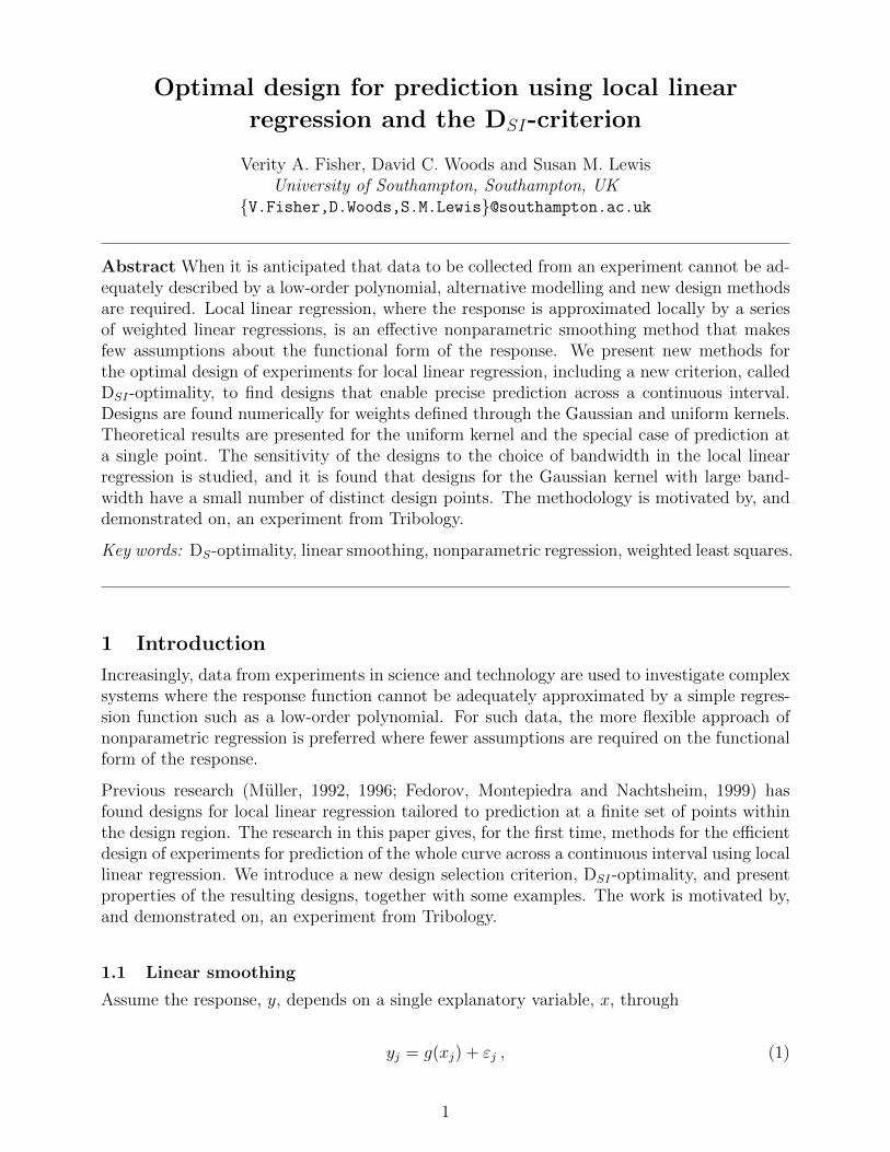
Data from one run of the process was obtained by measuring the total wear of the disc andpin at a given number of time points after the disc has started spinning. The data fromdifferent runs of the process may differ due to random variation and the various differentsettings chosen for the controllable factors which included disc material, pin material and theaddition of various contaminants to the lubricant. Data from two runs of the process areshown in Figure 1. Notice that wear can actually decrease at some time points due to a buildup of contamination in the groove, or “wear scar”, worn into the disc by the pin.

In this paper, we find optimal designs for predicting curves such as those given in Figure 1 us-ing only a small number of design points; that is, we choose the ‘best’ subset {x1, . . . , xn} ⊂ Rof points at which to observe the process. In Section 2 we describe prediction via the locallinear estimator. Section 3 introduces optimal design for this prediction method and, in par-ticular, DSI-optimal designs for predicting the curve across an interval. Results are presentedin Section 4 for the special case of prediction at a single point, as well as prediction acrossan interval. In Section 5, DSI-optimal designs are found for a simulated wear experiment,motivated by the Tribology application. We make our concluding remarks in Section 6.

2 Local linear regression

We employ local regression methods (Pelto, Elkins and Boyd, 1968 and Cleveland, 1979)to estimate g(·). Local fitting weights the observations to ensure that points closer (or morelocal) to x have larger influence on g(x). For prediction at a point x∗, local weighted regressionfits a pth degree polynomial using weighted least squares.

2

500 1000 1500 2000 25000.001

0.002

0.003

0.004

0.005

0.006

Time Index500 1000 1500 2000 2500

0.007

0.008

0.009

0.01

0.011

0.012

0.013

0.014

Time Index

Fig 1: Data from run 1 (left) and run 2 (right) of the wear experiment withexamples of a locally linear smooth fit (red)

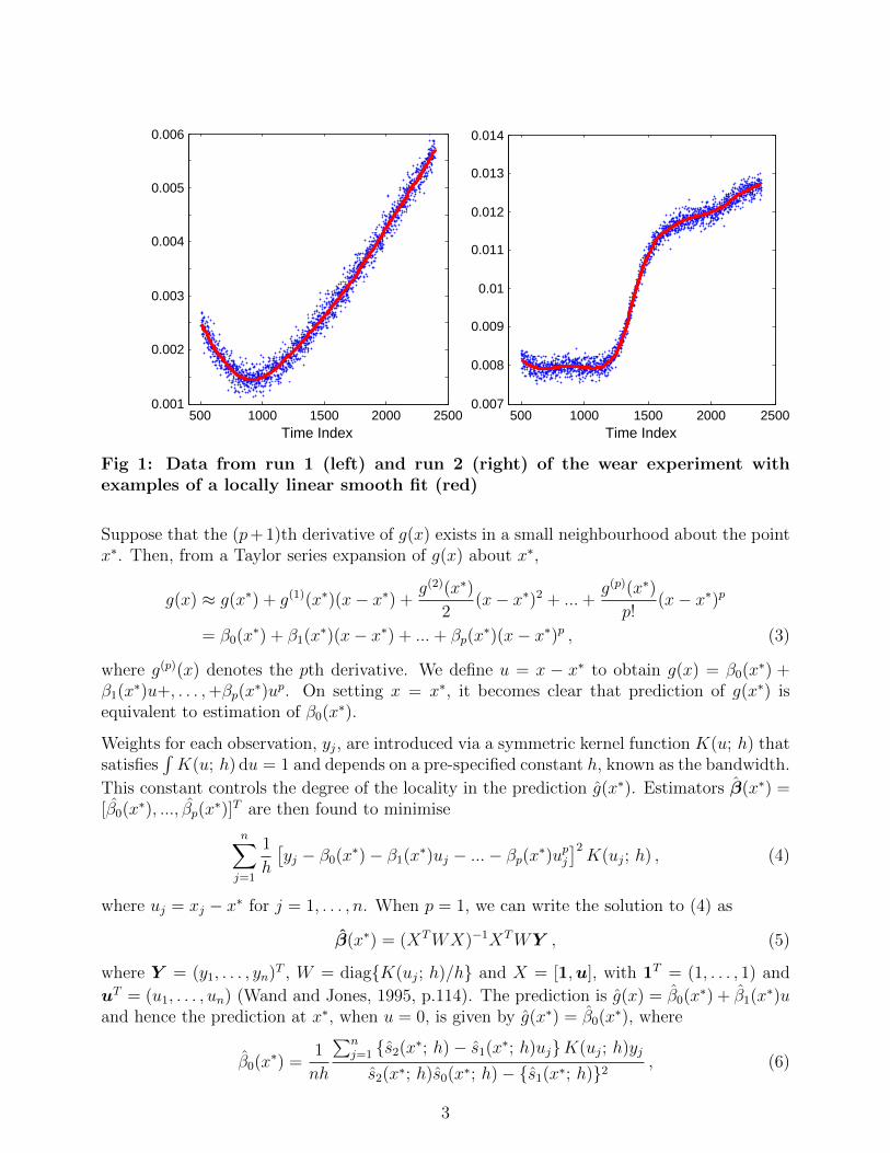
Suppose that the (p+ 1)th derivative of g(x) exists in a small neighbourhood about the pointx∗. Then, from a Taylor series expansion of g(x) about x∗,

g(x) ≈ g(x∗) + g(1)(x∗)(x− x∗) +g(2)(x∗)

2(x− x∗)2 + ...+

g(p)(x∗)

p!(x− x∗)p

= β0(x∗) + β1(x

∗)(x− x∗) + ...+ βp(x∗)(x− x∗)p , (3)

where g(p)(x) denotes the pth derivative. We define u = x − x∗ to obtain g(x) = β0(x∗) +

β1(x∗)u+, . . . ,+βp(x

∗)up. On setting x = x∗, it becomes clear that prediction of g(x∗) isequivalent to estimation of β0(x

∗).

Weights for each observation, yj, are introduced via a symmetric kernel function K(u; h) thatsatisfies

∫K(u; h) du = 1 and depends on a pre-specified constant h, known as the bandwidth.

This constant controls the degree of the locality in the prediction g(x∗). Estimators β(x∗) =[β0(x

∗), ..., βp(x∗)]T are then found to minimise

n∑j=1

1

h

[yj − β0(x∗)− β1(x∗)uj − ...− βp(x∗)upj

]2K(uj; h) , (4)

where uj = xj − x∗ for j = 1, . . . , n. When p = 1, we can write the solution to (4) as

β(x∗) = (XTWX)−1XTWY , (5)

where Y = (y1, . . . , yn)T , W = diag{K(uj; h)/h} and X = [1,u], with 1T = (1, . . . , 1) and

uT = (u1, . . . , un) (Wand and Jones, 1995, p.114). The prediction is g(x) = β0(x∗) + β1(x

∗)uand hence the prediction at x∗, when u = 0, is given by g(x∗) = β0(x

∗), where

β0(x∗) =

1

nh

∑nj=1 {s2(x∗; h)− s1(x∗; h)uj}K(uj; h)yj

s2(x∗; h)s0(x∗; h)− {s1(x∗; h)}2, (6)

3

and sr(x∗; h) =

∑nk=1 u

rkK(uk; h)/(nh), for r = 0, 1, 2. From (2), the smoothing weights at

x∗ are given by

Sj(x∗) =

1

nh

∑nj=1 {s2(x∗; h)− s1(x∗; h)uj}K(uj; h)

s2(x∗; h)s0(x∗; h)− s1(x∗; h)2.

Note that when K(uj; h) = h for all uj, then β0(x∗) reduces to the ordinary least squares

estimator of the intercept in a simple linear regression. A further special case, the Nadaraya-Watson estimator (Nadaraya, 1964; Watson, 1964), is obtained when p = 0. Fan (1992)established the advantages of the local linear smoother (p = 1) over the Nadaraya-Watsonestimator in terms of expected squared error.

In this paper, we find designs for the uniform and Gaussian kernel functions:

Uniform: K(u; h) =

{0.5 if |u/h| ≤ 1 ,

0 otherwise .

Gaussian: K(u; h) =1√2π

exp

{− u2

2h2

}, −∞ < u <∞ .

We choose these kernels to demonstrate the differences in optimal designs for truncated andnon-truncated kernel functions. Clearly, both kernel functions are non-increasing functionsof |u| = |x− x∗|. For the uniform kernel, observations y with corresponding |x− x∗| > h willnot influence prediction at x. The Gaussian kernel function is monotonically decreasing withu2 but monotonically increasing with h. These two kernels present some different issues fordesign; for example, with a truncated kernel such as the uniform, at least two design pointsare required to lie within distance h of x∗ to enable the local linear smoother to be estimated.For both kernels, lower prediction variance is obtained when more design points lie within hof the point x.

3 Experimental design for local prediction

In this section, we define a design selection criterion, the DSI-criterion, for prediction of g(x∗)for x∗ ∈ I = [a, b] ⊂ R using local linear smoothing. We find designs ξn = {x1, ..., xn}, withx1 ≤ . . . ≤ xn.

Similar problems were considered by Muller (1992), Muller (1996) and Fedorov et al. (1999)for local linear regression. Muller (1992) and Muller (1996) found designs that minimised aweighted sum of variances of the estimator β0(xi), for prediction at points x∗i , i = 1, ..., q:

ΨM(ξ) = trace

{q∑i=1

Ai(XTi WiXi)

−1

}, (7)

where Ai = aiA, ai is a given scalar and A = e1eT1 with e1 the first column of a p× p identity

matrix. The p× p matrix, XTi WiXi, is the information matrix for the linear model

Y = Xiβ(x∗i ) + η , (8)

4

where Xi = [1n,ui, . . . ,upi ], u

Ti = (ui1, . . . , uin) and uij = xj − x∗i . The n-vector η ∼

N(0,W−1), with W the diagonal matrix of kernel weights. That is, (8) is the linear modelthat would lead to estimators (5) of β(xi). Muller (1992) found designs by maximising (7)for examples when prediction was required at a set of q = 9 equally spaced points in [−1, 1]and when x could only take values from this same set.

Fedorov et al. (1999) also found designs for local linear smoothing but adopted a mean squarederror criterion where the true model was assumed to be a local linear regression of higher order.We follow Muller (1992) and make the assumption that sufficient prior information is availableto choose an appropriate value of h to render the bias negligible.

Designs for alternative local smoothing methods have been considered by Cheng, Hall andTitterington (1998) and Biedermann and Dette (2001), among other authors.

3.1 DSI-optimal designs for prediction

Our design selection criterion is motivated by model (8). Under this model, and using notationthat suppresses the dependence of X and W on x∗, the variance-covariance matrix of β(x∗)is given from equation (5) by

Var(β(x∗)

)= σ2(XTWX)−1XTWW−1WX(XTWX)−1

= σ2(XTWX)−1 , (9)

with corresponding information matrix M(ξn) = XTWX.

For the prediction of g(x∗), interest is only in β0(x∗). Hence, we apply DS-optimality (see,

for example, Atkinson et al., 2007), which selects designs that minimise the variance of asubset of model parameter estimators whilst regarding the remaining parameters as nuisanceparameters. The information matrix can be partitioned as

M(ξn) = XTWX

=

[M11(ξn) M12(ξn)M21(ξn) M22(ξn)

]=

1

h

[ ∑nj=1K (uj;h)

∑nj=1 ujK (uj;h)∑n

j=1 ujK (uj;h)∑n

j=1 u2jK (uj;h)

].

In general, the DS-optimality criterion seeks a design that minimises the determinant ofM−1

11 (ξn) or, equivalently, maximises

|M11(ξn)−M12(ξn)M−122 M

T12(ξn)| = |M(ξn)|

|M22(ξn)|.

For local linear regression, and estimation of β0(x∗),

|M(ξn)| = |XTWX| =

[1

h

n∑j=1

K (uj; h)

][1

h

n∑j=1

u2jK (uj; h)

]−

[1

h

n∑j=1

ujK (uj; h)

]2,

5

and

|M22(ξn)| = 1

h

n∑j=1

u2jK (uj; h) .

Hence, a DS-optimal design for prediction at a point x∗ for local linear regression maximisesthe objective function

ΨS(ξn) =

∑nj=1K (uj; h)

∑nj=1 u

2jK (uj; h)− [

∑nj=1 ujK (uj; h)]2

h∑n

j=1 u2jK (uj; h)

. (10)

This objective function is equivalent to (7) with q = 1.

To select designs for predicting the whole curve over an interval, we construct a compoundcriterion (Atkinson et al., 2007, ch.21) by integrating (10) across I = [a, b].

Definition 1: A DSI-optimal design ξ∗n for prediction across the interval [a, b] for local linearregression maximises

ΨSI(ξn) =1

h

∫ b

a

log

n∑j=1

K (xj − x∗; h)−

[∑nj=1

(xj−x∗h

)K (xj − x∗; h)

]2∑n

j=1

(xj−x∗h

)2K (xj − x∗; h)

dx∗

=

∫ b

a

log [L(x∗)] dx∗ , (11)

where

L(x∗) =1

h

n∑j=1

K (xj − x∗; h)−

[∑nj=1

(xj−x∗h

)K (xj − x∗; h)

]2∑n

j=1

(xj−x∗h

)2K (xj − x∗; h)

.

We integrate the logarithm of (10) as an alternative to integrating the DS-efficiency across[a, b]. Here taking logs compensates for any differences in scale in (10) for different values ofx∗ (see also Woods et al., 2006).

Note that we do not restrict the design region to be the interval [a, b] (cf Box and Draper,1959 and the concept of the operability region). However, most DSI-optimal designs have allpoints within, or close to, the interval [a, b].

Evaluation of (11) is analytically intractable for both the uniform and Gaussian kernels andhence we find designs by applying a Legendre-Gauss quadrature approximation (see Golub andWelsch, 1969). Thus, we maximise a weighted sum of the logarithm of objective function (10)at pa abscissa values,

ΨSI(ξn) ≈pa∑i=1

κi log [L(x∗i )] , (12)

where x∗i are chosen as solutions to the Legendre polynomials and κi are Legendre-Gaussweights. By comparing values of (12) calculated using different values of pa, we concludedthat pa = 25 was a sufficient in most cases (including for large n); a value of pa = 500 wasused for a few, more difficult, integrals.

6

4 Theoretical and numerical results

In this section, we apply the DSI-criterion to find designs for different values of run sizes n.First, we consider the special case of DS-optimality for predicting at a single point x∗, wheresome theoretical results on optimal designs can be derived.

4.1 Designs for prediction at a single point

We now derive sufficient conditions for a design to be DS-optimal, i.e. maximising (10), forprediction at a single point using local linear regression. We then demonstrate the results forthe uniform kernel. Our discussion of the Gaussian kernel is delayed to Section 4.2 where weapply DSI-optimality. We first prove a simple but useful result.

Lemma 1. An upper bound, U , for objective function (10) is given by

U =n

hK(0; h) ≥ max

ξn∈Dn

{ΨS(ξn)} .

where Dn is the set of all possible designs of run size n.

Proof. By definition, K(0; h) is the maximum value ofK. Hence, K (uj; h) = [K(0; h)− f(uj)]where f(x) ≥ 0 for all x and f(0) = 0 . Hence (10) can be expressed as

ΨS(ξn) =1

h

(n∑j=1

[K(0; h)− f(uj)]−[∑n

j=1 ujK(uj; h)]2∑nj=1 u

2jK(uj; h)

).

As the kernel is a non-negative function,

[∑n

j=1 ujK(uj; h)]2∑nj=1 u

2jK(uj; h)

> 0 ,

and hence

ΨS(ξ) =1

h

(n∑j=1

[K(0; h)− f(uj)]−[∑n

j=1 ujK (uj; h)]2∑nj=1 u

2jK (uj; h)

)(13)

≤ 1

h

n∑j=1

[K(0; h)− f(uj)]

=1

h

n∑j=1

K(0; h)− 1

h

n∑j=1

f(uj)

≤ n

hK(0; h) . (14)

Lemma 1 leads directly to a sufficient condition for a design to be DS-optimal.

Theorem 1. A sufficient condition for design ξ∗n to be DS-optimal for prediction at a singlepoint using local linear regression is that ΨS(ξ∗n) = nK(0; h)/h.

Proof. Proof follows directly from Lemma 1.

7

4.1.1 Optimal designs using the uniform kernel

We now find DS-optimal designs for prediction at a single point under the uniform kernel.Using this kernel, objective function (10) simplifies to:

ΨS(ξn) =1

2h

[n∑j=1

1A(uj)−[∑n

j=1 uj1A(uj)]2∑n

j=1 u2j1A(uj)

], (15)

where

1A(uj) =

{1 if uj ∈ A,0 otherwise ,

andA = {uj; |uj| ≤ h} . (16)

It is straightforward to establish the form of DS-optimal designs that maximise (15) as acorollary to Theorem 1.

Corollary 1. For the uniform kernel and prediction at x∗, a design ξn = {x1, . . . , xn} withn ≥ 2 that satisfies

(i) |xj − x∗| ≤ h for j = 1, . . . , n

(ii) x =∑n

j=1 xj/n = x∗

(iii)∑n

j=1(xj − x)2 > 0

has ΨS(ξn) = n2h

and is DS-optimal.

Proof. Conditions (i)-(iii) imply that (a) 1A(uj) = 1 for all j = 1, . . . , n, (b)∑n

j=1(xj−x∗) = 0,

and (c)∑n

j=1(xj − x∗)2 > 0. Hence, it follows from the form of (15) that

ΨS(ξ∗n) =nK(0; h)

h=

n

2h. (17)

The DS-optimality of the design follows directly from Theorem 1.

The result from Corollary 1 was verified numerically by finding a variety of DS-optimal designsvia minimisation of −ΨS(ξn) using the fminsearch and ksrlin routines in MATLAB (2010)and the Nelder-Mead algorithm (Nelder and Mead, 1965). Every design found satisfied theconditions in Corollary 1, with ΨS(ξn) = n/2h. Fedorov et al. (1999) found designs under amean squared error criterion for the uniform kernel on [−1, 1] with h = 2. For this choiceof kernel and bandwidth, every design point in [−1, 1] has equal weight for prediction at anypoint in x∗ ∈ [−1, 1]. Their design had equally replicated support points {−1, 1} and, fromCorollary 1, this design is also DS-optimal.

4.2 Designs for prediction across an interval

We apply the DSI-optimality criterion using local linear regression. For the numerical results,we take the interval [−1, 1], that is a = −1 and b = 1. Designs for predicting at a finitenumber of given points can be found in Fisher (2012).

8

Table 1: DSI-optimal designs for prediction over [−1, 1] using a uniform kernel forn design points and bandwidth h

n h = 0.212 ±0.08 ±0.27 ±0.45 ±0.62 ±0.80 ±0.9815 ±1.00 ±0.83 ±0.68 ±0.54 ±0.38 ±0.24 ±0.11 0.00

h = 0.55 ±1.00 ±0.50 0.006 ±0.99 ±0.55 ±0.207 ±1.03 ±0.61 ±0.30 0.008 ±1.04 ±0.71 ±0.39 ±0.1612 ±1.12 ±0.86 ±0.65 ±0.45 ±0.27 ±0.0615 ±1.12 ±0.95 ±0.78 ±0.54 ±0.40 ±0.30 ±0.17 0.00

h = 0.754 ±0.94 ±0.255 ±1.09 ±0.53 0.006 ±1.10 ±0.63 ±0.137 ±1.10 ±0.82 ±0.22 0.008 ±1.17 ±0.83 ±0.46 ±0.0812 ±1.18 ±1.04 ±0.80 ±0.55 ±0.16 ±0.0515 ±1.20 ±1.09 ±0.90 ±0.70 ±0.52 ±0.18 ±0.10 0.00

h = 13 ±1.00 0.004 ±1.12 ±0.325 ±1.16 ±0.52 0.006 ±1.19 ±0.65 ±0.307 ±1.30 ±0.85 ±0.36 0.008 ±1.30 ±0.90 ±0.47 ±0.2412 ±1.34 ±1.10 ±0.82 ±0.52 ±0.37 ±0.2115 ±1.38 ±1.17 ±0.97 ±0.72 ±0.51 ±0.38 ±0.25 0.00

9

4.2.1 DSI-optimal designs for the uniform kernel

Table 1 gives DSI-optimal and efficient designs found by numerical search for the uniformkernel and a variety of values of n and h. The choices of n and h were restricted to ensureadequate numbers of points in each sub-interval [x−h, x+h] (with x−h ≥ −1 and x+h ≤ 1).For example, when h = 0.2 at least 11 points are required to predict over an interval of lengthtwo. In general, the minimum number of design points required is given by

nmin =b− ah

+ 1 , (18)

The designs found are all symmetric about 0, resulting from the symmetry of the kernelfunction and the prediction interval. The points span an interval just wider than the predictioninterval [−1, 1] and, although well spread across the interval, they are not equally spaced.Generally, the range of the design points increases with n; the pattern with changing h is lessclear. For smaller n and larger h, the numerical optimisation was more straightforward andfaster.

4.3 DSI-optimal designs using the Gaussian kernel

As in the previous section, Table 2 presents DSI-optimal designs for the Gaussian kernelfound via numerical search. Once again all the designs are symmetric about 0, due to the

Table 2: DSI-optimal designs for prediction over [−1, 1] using a Gaussian kernel forn design points and bandwidth h. When design points are repeated, the numberof repetitions is given in parentheses

n h = 0.2 h = 0.52 ±0.16 ±0.653 ±0.72 0.00 ±0.88 0.004 ±0.88 ±0.31 ±0.96 ±0.315 ±0.92 ±0.46 0.00 ±1.00 ±0.53 0.006 ±0.93 ±0.54 ±0.18 ±0.88(2) 0.00(2)7 ±0.95 ±0.59 ±0.30 0.00 ±0.92(2) ±0.27 0.008 ±0.96 ± 0.64 ±0.39 ±0.12 ±0.95(2) ±0.50 0.00(2)12 ±0.98 ±0.85 ±0.52(2) ±0.17(2) ±0.88(4) 0.00(4)15 ±0.95(2) ±0.61(2) ±0.43 ±0.20(2) 0.00 ±0.88(5) 0.00(5)

h = 0.75 h = 12 ±0.77 ±0.873 ±0.98 0.00 ±1.09 0.004 ±0.86 ±0.68 ±0.87(2)5 ±0.88(2) 0.00 ±0.99 0.006 ±0.85(2) ±0.60 ±0.87(3)7 ±0.85(3) 0.00 ±0.95(3) 0.008 ±0.85(3) ±0.52 ±0.87(4)12 ±0.84(5) ±0.33 ±0.87(6)15 ±0.81(7) 0.00 ±0.90(7) 0.00

10

symmetry of both the kernel function and prediction interval. However, for larger values of h,the designs now have substantial numbers of repeated points. Larger values of h represent lesslocal behaviour, and hence fewer support points are required. Large values of h also resultin design points closer to the extremes of [−1, 1]; for larger h, these points will still havesubstantial weight for predictions near the centre of the interval. However, unlike designs forthe uniform kernel, no points from these designs lie outside the prediction interval.

To assess the robustness of designs to the choice of kernel function, we calculate the efficiencyunder the Gaussian kernel of a design found assuming the uniform kernel would be used forthe modelling. The efficiency is given by

Eff = exp{

ΨG(ξu)−ΨG(ξG)},

where ΨG(ξu) and ΨG(ξG) are the respective values of objective function (12) calculated usingthe Gaussian kernel for two designs: (a) ξu, the DSI-optimal design under the uniform kernel;and (b) ξG, the DSI-optimal design using the Gaussian kernel. Two examples are considered:(i) h = 0.5 and n = 5 and (ii) h = 0.5 and n = 15. For both cases, design ξu can be found inTable 1 and ξG in Table 2. For case (i), the two designs have very similar design points andthe uniform kernel design has very high efficiency of 0.998. For case (ii), the uniform designhas a substantially greater number of distinct design points than the design found using theGaussian kernel but still has high efficiency of 0.932.

In general, designs found for the Gaussian kernel may not perform well under the uniformkernel, especially for large n, as they have fewer than nmin distinct design points. Hence,designs for the uniform kernel are more robust to the choice of kernel function.

5 Application to the tribology experiment

We now demonstrate the DSI-criterion using simulated data sets motivated by the Tribologyexperiment and assess the performance of the resulting designs. Recall that the aim of theexperiment was to predict the wear curve over an interval. For each of the two runs of theprocess (Figure 1), the original data sets had 1900 data points, to which we fit local linearregression models. The bandwidths, h = 0.2 and h = 0.1 for runs 1 and 2, respectively, werechosen “by eye” to achieve adequate descriptions of the mean response.

DSI-optimal designs for these two bandwidths are given in Table 3 for the Gaussian kerneland a variety of values of n. For design selection, we scaled the prediction interval to [−1, 1].Notice once again the symmetry of the designs. For these relatively complex curves andsmaller bandwidths, the optimal designs have many distinct points; the designs for h = 0.1have more distinct points than the designs for h = 0.2.

To allow assessment of the performance of these designs relative to using all the points in theoriginal data set, we simulate wear observations from independent normal distributions withmean given by the local linear regressions (Figure 1) and variance 2.25×10−8, commensuratewith background variability exhibited by the process. We then compared the local linearregression models obtained from the DSI-optimal designs and the whole data sets. Figure 2shows the smoothed fits for these runs, using h = 0.2 and h = 0.1, respectively, for both thewhole data set and the data from the corresponding DSI-optimal designs with n = 25 (run1) and n = 30 (run 2).

11

Table 3: Further DSI-optimal designs for predicting over [−1, 1] using a Gaussiankernel for n design points and bandwidth h. When design points are repeated,the number of repetitions is given in parentheses

n h = 0.115 ±0.98 ±0.81 ±0.67 ±0.53 ±0.40 ±0.27 ±0.13 0.0020 ±0.99 ±0.87 ±0.75 ±0.66 ±0.55 ±0.45 ±0.35 ±0.25

±0.15 ±0.0525 ±0.99 ±0.94 ±0.77(2) ±0.63 ±0.58 ±0.48 ±0.41 ±0.32

±0.24 ±0.16 ±0.08 0.0030 ±0.98(2) ±0.81(2) ±0.71 ±0.60(2) ±0.50 ±0.42 ±0.39 ±0.26(2)

±0.16 ±0.09 ±0.05

h = 0.215 ±0.95(2) ±0.61(2) ±0.43 ±0.20(2) 0.0020 ±0.94(3) ±0.57(3) ±0.38 ±0.1625 ±0.96(3) ±0.79 ±0.54(4) ±0.21(3) 0.16

For run 1, the prediction from the DSI-optimal design with n = 25 points slightly over-predictsfor x ∈ [600, 1200]. The choice of h = 0.2 for this run perhaps over-smoothes the data in thissub-interval. However, a smaller choice of h leads to under-smoothing for larger values of x.For run 2, the DSI-optimal design with h = 0.1 and n = 30 provides a reasonably accuratefit.

To assess quantitatively the performance of the DSI-optimal designs, we calculated “movingwindow” mean squared errors (MSEs):

δi =k=i+100∑k=i−100

[g(xk)− yk]2 , i = 101, . . . , 1800 . (19)

For each run, (19) was calculated for the whole data set, labelled δi(w), and the DSI-optimaldesign, labelled δ(ξ). For an overall comparison, we used the average standardised difference

∆ =1

1700

1800∑i=101

∆i ,

where

∆i =δi(ξ)− δi(w)

δi(ξ). (20)

In all these comparisons, it should be recognised that a DSI-optimal design was found tominimise the prediction variance and not the mean squared error.

For run 1, Figure 3 shows the fitted curves from DSI-optimal designs with n = 15, 20, 25points and h = 0.2, the fitted curves for the whole data set, and plots of δi for the optimaldesigns and the whole data set. Figure 4 gives equivalent plots for run 2 with DSI-optimaldesigns for n = 15, 20, 25, 30 points and h = 0.1.

For both runs, there is little qualitative difference between the regression curves for the optimaldesigns with different numbers of runs (Figures 3(a) and 4(a)). The moving window MSEs,

12

400 600 800 1000 1200 1400 1600 1800 2000 2200 24000

0.001

0.002

0.003

0.004

0.005

0.006

0.007

x

Run 1

400 600 800 1000 1200 1400 1600 1800 2000 2200 24000.007

0.008

0.009

0.01

0.011

0.012

0.013

0.014

x

Run 2

Fig 2: Simulated data (small blue dots) and DSI-optimal designs (large blackdots) for n = 25 (run 1) and n = 30 (run 2) with smooth fitted curves using thewhole data set (red) and the data from the design points (black)

13

500 1000 1500 2000 25001

2

3

4

5

6x 10−3

x

(a)

500 1000 1500 2000 25001

2

3

4

5

6x 10−3

x

(b)

500 1000 1500 2000 25000

0.2

0.4

0.6

0.8

1

1.2x 10−5

x

MS

E

(d)

500 1000 1500 2000 25000

0.2

0.4

0.6

0.8

1

1.2x 10−5

x

MS

E

(c)

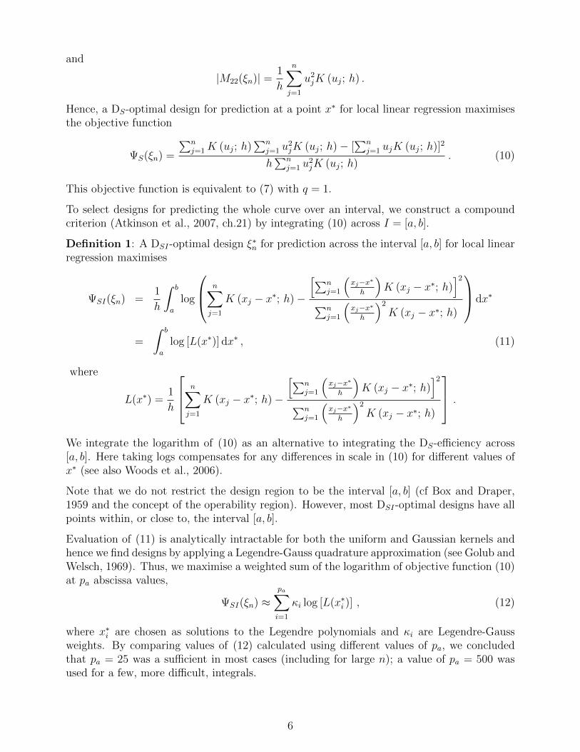
Fig 3: Run 1: Smooth fits from local linear regressions and MSE plots (a) g(x)using data corresponding to DSI-optimal designs with 15 (blue), 20 (green) and25 (red) design points, (b) g(x) for the whole data set, (c) MSE for g(x) for 15,20 and 25 design points and (d) MSE for g(x) for the whole data set

δi, for each design (Figures 3(c) and 4(c)) are two-or three-orders of magnitude smaller thanthe mean predictions, reflecting the strong signal to noise ratio. The MSE for the whole dataset for each run (Figures 3(d) and 4(d)) is of similar magnitude to that obtained from theoptimal designs. The common peaks in the plots for δi, in the sub-interval [600, 1200] for run1 and [1000, 1500] for run 2, are indicative of areas where prediction is harder, for examplewhere the curve has its steepest slope for run 2.

The average standardised difference ∆ is smallest for run 1, ∆ = 0.189, when n = 15, andsmallest for run 2, ∆ = 0.166, when n = 25. While it would be expected that larger designswould produce smaller values of ∆, it should be noted that these results are for a singlesimulated set of data. A larger simulation study would likely produce more intuitive results.

5.1 Robustness of prediction to bandwidth selection

In general, there is likely to be some uncertainty in the correct choice of bandwidth h whendesigning an experiment. Even when studying run 1 and run 2, with data available, thischoice was not completely clear. To assess the robustness of the quality of the model fit fromDSI-optimal designs to the choice of h, we use run 2 and compare predictions from usingthe whole data set and h = 0.1 (considered the best “by eye” choice of bandwidth) to thepredictions obtained from optimal designs found for h = 0.2 and h = 0.3.

14

500 1000 1500 2000 25000.007

0.008

0.009

0.01

0.011

0.012

0.013

0.014

x

(a)

500 1000 1500 2000 25000.007

0.008

0.009

0.01

0.011

0.012

0.013

0.014

x

(b)

500 1000 1500 2000 25000

0.5

1

1.5

2x 10−5

x

MS

E

(d)

500 1000 1500 2000 25000

0.5

1

1.5

2x 10−5

x

MS

E

(c)

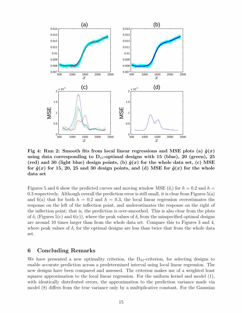
Fig 4: Run 2: Smooth fits from local linear regressions and MSE plots (a) g(x)using data corresponding to DSI-optimal designs with 15 (blue), 20 (green), 25(red) and 30 (light blue) design points, (b) g(x) for the whole data set, (c) MSEfor g(x) for 15, 20, 25 and 30 design points, and (d) MSE for g(x) for the wholedata set

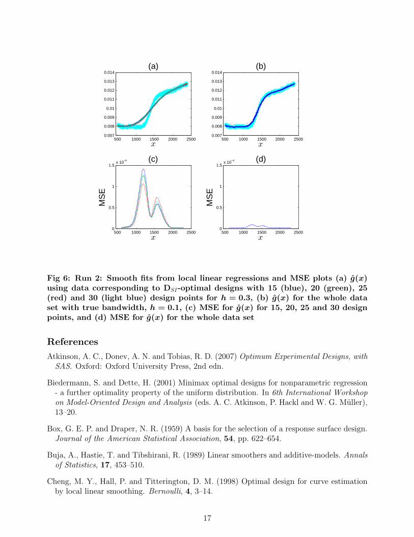
Figures 5 and 6 show the predicted curves and moving window MSE (δi) for h = 0.2 and h =0.3 respectively. Although overall the prediction error is still small, it is clear from Figures 5(a)and 6(a) that for both h = 0.2 and h = 0.3, the local linear regression overestimates theresponse on the left of the inflection point, and underestimates the response on the right ofthe inflection point; that is, the prediction is over-smoothed. This is also clear from the plotsof δi (Figures 5(c) and 6(c)), where the peak values of δi from the misspecified optimal designsare around 10 times larger than from the whole data set. Compare this to Figures 3 and 4,where peak values of δi for the optimal designs are less than twice that from the whole dataset.

6 Concluding Remarks

We have presented a new optimality criterion, the DSI-criterion, for selecting designs toenable accurate prediction across a predetermined interval using local linear regression. Thenew designs have been compared and assessed. The criterion makes use of a weighted leastsquares approximation to the local linear regression. For the uniform kernel and model (1),with identically distributed errors, the approximation to the prediction variance made viamodel (8) differs from the true variance only by a multiplicative constant. For the Gaussian

15

500 1000 1500 2000 25000.007

0.008

0.009

0.01

0.011

0.012

0.013

0.014

x

(a)

500 1000 1500 2000 25000.007

0.008

0.009

0.01

0.011

0.012

0.013

0.014

x

(b)

500 1000 1500 2000 25000

1

2

3

4

5

6

7

8x 10−5

x

MS

E

(d)

500 1000 1500 2000 25000

1

2

3

4

5

6

7

8x 10−5

x

MS

E

(c)

Fig 5: Run 2: Smooth fits from local linear regressions and MSE plots (a) g(x)using data corresponding to DSI-optimal designs with 15 (blue), 20 (green), 25(red) and 30 (light blue) points for h = 0.2, (b) g(x) for the whole data set withtrue bandwidth, h = 0.1, (c) MSE for g(x) for 15, 20, 25 and 30 design points,and (d) MSE for g(x) for the whole data set

kernel, the approximation also makes an adjustment to the bandwidth.

A clear direction for future work, motivated by the Tribology application, is to find designsthat assume a varying bandwidth across the prediction interval. Such models and designswould be better able to approximate responses that display marked differences in smoothness.

Acknowledgments

This work was supported by the UK Engineering and Physical Sciences Research Councilthrough a PhD studentship (Fisher) and a Fellowship (Woods; EP/J018317/1). The au-thors thank Professor Robert Wood, Dr Ling Wang and Dr Terry Harvey (National Centrefor Advanced Tribology, University of Southampton) and Dr Ramkumar Penchaliah (IndianInstitute of Technology Madras) for providing the data for the example, and for related dis-cussions. The authors also acknowledge the use of the IRIDIS High Performance ComputingFacility, and associated support services at the University of Southampton, in the completionof this work.

16

500 1000 1500 2000 25000.007

0.008

0.009

0.01

0.011

0.012

0.013

0.014

x

(a)

500 1000 1500 2000 25000.007

0.008

0.009

0.01

0.011

0.012

0.013

0.014

x

(b)

500 1000 1500 2000 25000

0.5

1

1.5x 10−4

x

MS

E

(d)

500 1000 1500 2000 25000

0.5

1

1.5x 10−4

x

MS

E

(c)

Fig 6: Run 2: Smooth fits from local linear regressions and MSE plots (a) g(x)using data corresponding to DSI-optimal designs with 15 (blue), 20 (green), 25(red) and 30 (light blue) design points for h = 0.3, (b) g(x) for the whole dataset with true bandwidth, h = 0.1, (c) MSE for g(x) for 15, 20, 25 and 30 designpoints, and (d) MSE for g(x) for the whole data set

References

Atkinson, A. C., Donev, A. N. and Tobias, R. D. (2007) Optimum Experimental Designs, withSAS. Oxford: Oxford University Press, 2nd edn.

Biedermann, S. and Dette, H. (2001) Minimax optimal designs for nonparametric regression- a further optimality property of the uniform distribution. In 6th International Workshopon Model-Oriented Design and Analysis (eds. A. C. Atkinson, P. Hackl and W. G. Muller),13–20.

Box, G. E. P. and Draper, N. R. (1959) A basis for the selection of a response surface design.Journal of the American Statistical Association, 54, pp. 622–654.

Buja, A., Hastie, T. and Tibshirani, R. (1989) Linear smoothers and additive-models. Annalsof Statistics, 17, 453–510.

Cheng, M. Y., Hall, P. and Titterington, D. M. (1998) Optimal design for curve estimationby local linear smoothing. Bernoulli, 4, 3–14.

17

Cleveland, W. S. (1979) Robust locally weighted regression and smoothing scatterplots. Jour-nal of the American Statistical Association, 74, 829–836.

Fan, J. Q. (1992) Design-adaptive nonparametric regression. Journal of the American Statis-tical Association, 87, 998–1004.

Fedorov, V. V., Montepiedra, G. and Nachtsheim, C. J. (1999) Design of experiments forlocally weighted regression. Journal of Statistical Planning and Inference, 81, 363–382.

Fisher, V. A. (2012) Optimal and efficient experimental design for nonparametric regressionwith application to functional data. Ph.D. thesis, University of Southampton, UK.

Golub, G. H. and Welsch, J. H. (1969) Calculation of Gauss quadrature rules. Mathematicsof Computation, 23, 221–230.

MATLAB (2010) Version 7.10.0 (R2010a). The MathWorks Inc., Natick, Massachusetts.

Muller, W. G. (1992) Optimal design for moving local regressions, unpublished technicalreport. URL http://epub.wu.ac.at/932/ (accessed 09/12/12).

— (1996) Optimal design for local fitting. Journal of Statistical Planning and Inference, 55,389–397.

Nadaraya, E. A. (1964) On estimating regression. Theory of Probability and its Applications,10, 186–190.

Nelder, J. and Mead, R. (1965) A simplex method for function minimization. The ComputerJournal, 7, 308–313.

Pelto, C. R., Elkins, T. A. and Boyd, H. A. (1968) Automatic contouring of irregularly spaceddata. Geophyisics, 33, 424–430.

Ramsay, J. O. and Silverman, B. (2005) Functional Data Analysis. New York: Springer, 2ndedn.

Simonoff, J. S. (1996) Smoothing Methods in Statistics. New York: Springer-Verlag.

Wand, M. P. and Jones, M. (1995) Kernel Smoothing. London: Chapman and Hall.

Watson, G. S. (1964) Smooth regression analysis. Sankhya A, 26, 101–116.

Woods, D. C., Lewis, S. M., Eccleston, J. A. and Russell, K. G. (2006) Designs for generalizedlinear models with several variables and model uncertainty. Technometrics, 48, 284–292.

18