International Journal of Fracture manuscript No.(will be inserted by the editor)

On fracture testing of piezoelectric ceramics

Yael Motola · Leslie Banks-Sills · Victor

Fourman

Received: date / Accepted: date

Abstract Fracture tests carried out on unpoled and poled PZT-5H four-point bend

specimens are presented in this paper. The crack faces were parallel to the poling di-

rection. Both mechanical loads and electric fields were applied to the poled specimens.

The experimental results were analyzed by means of the finite element method and a

conservative M -integral including the crack face boundary conditions. Fracture tests

on four-point bend PIC-151 specimens with the crack faces perpendicular to the pol-

ing directions were also analyzed here; the experimental results were taken from the

literature. A mixed mode fracture criterion is proposed for piezoelectric ceramics. This

criterion is based upon the energy release rate and two phase angles. This criterion was

implemented with experimental results from the literature and from this investigation.

Excellent agrement was found between the fracture curve and the experimental re-

sults of the specimens with the crack faces perpendicular to the poling direction. With

some scatter, reasonable agreement was observed between the fracture curve and the

experimental results of the specimens with crack faces parallel to the poling direction.

Keywords piezoelectric ceramics · fracture tests · intensity factors · energy release

rate · M -integral · fracture criterion · finite element method

1 Introduction

Piezoelectric ceramics are in widespread use as sensors and actuators in smart struc-

tures, despite the absence of a fundamental understanding of their fracture behavior.

Piezoceramics are brittle and susceptible to cracking. As a result of the importance

The Dreszer Fracture Mechanics LaboratorySchool of Mechanical EngineeringFaculty of EngineeringTel Aviv UniversityRamat Aviv 69978, IsraelTel.: +972-3-640-8132Fax: +972-3-640-7617E-mail: ymotola@eng.tau.ac.il, banks@eng.tau.ac.ilAppears in: International Journal of Fracture, 159 (2009) 167–190, DOI 10.1007/s10704-009-9392-x.

2

of the reliability of these devices, there has been tremendous interest in studying the

fracture and failure behavior of such materials. To understand failure mechanisms of

piezoelectric materials and maintain the stability of cracked piezoelectric structures

operating in an environment of combined electro-mechanical loading, analysis of its

mechanical and electrical behavior is a prerequisite.

One of the key problems in properly analyzing fracture behavior of piezoelectric

ceramics is selection of the correct boundary conditions on the crack faces. There have

been four possible sets of boundary conditions presented in the literature, i.e. imper-

meable, permeable, semi-permeable and energetically consistent boundary conditions.

With the impermeable crack assumption, the permittivity of the gap is taken to be

zero. This implies that the normal component of the electric flux density must vanish

there (Deeg 1980). In contrast, with the permeable model, the crack is assumed not

to perturb the electric field so that both the electric potential and normal electric flux

density are continuous across the crack faces (Parton 1976). Semi-permeable boundary

conditions were proposed by Hao and Shen (1994), in which the electric permeability

in the crack gap is accounted for. In each of these three models, it is assumed that the

crack faces are traction free. Landis (2004) proposed a new set of boundary conditions

that consists of the semi-permeable electric boundary conditions and additional crack

closing tractions; these conditions are called the energetically consistent boundary con-

ditions. Application of the energetically consistent boundary conditions on the crack

faces solved the problem that McMeeking (2004) found in which the energy release

rate calculated far from the crack tip and in its vicinity for semi-permeable conditions

differed. In this study, energetically consistent boundary conditions are employed.

There have been various experimental techniques used in conducting fracture tests

on piezoelectric materials. They include compact tension, three and four-point bend-

ing tests, indentation fracture techniques and the double torsion test (Qin 2001). Many

tests have been carried out with the indentation technique (Tobin and Pak 1993; Lynch

1998; Shindo et al. 2001; Schneider et al. 2003). For many fracture experiments, po-

larized piezoelectric ceramics have been treated to be isotropic and use was made of

purely mechanical calibrations for the stress intensity factor KI (Freiman et al. 1974;

Bruce et al. 1978; McHenry and Koepke 1983; Pohanka et al. 1983; Tobin and Pak 1993;

Zhang et al. 2004). The fracture toughness obtained in this way may be defined as the

apparent fracture toughness and is typically referred to as KIc in the literature. This

parameter is influenced by the relation between the mechanical and electrical loads.

The apparent fracture toughness for a crack parallel to the poling direction was found

to be higher than that obtained for a crack perpendicular to the poling direction (Pis-

arenko et al. 1985; Tobin and Pak 1993; Shindo et al. 2001; Zhang et al. 2004). However,

this parameter by itself should not be used to predict fracture of poled material.

There are conflicting experimental results in the literature for the electric field

effect on crack propagation. It was found that a positive electric field promoted crack

propagation and a negative electric field inhibited it (Tobin and Pak 1993; Lynch 1998;

Park and Sun 1995a; Shindo et al. 2001); whereas the opposite trends were observed

by Wang and Singh (1997) and Shindo et al. (2005). Perhaps, the difference between

the behavior of the results obtained by Wang and Singh (1997) and others is related

to the material which was tested. Shindo et al. (2005) examined composite PZT-metal

specimens; hence, this may explain the difference in the results.

An important study which shows how to assess the behavior of the air within a

crack was carried out by Schneider et al. (2003). The electric potential difference across

cracks formed by indentation in PZT was measured by means of a Kelvin probe. For

3

this particular problem, the permittivity of the medium within the cavity was found

to be κa = 40κ0, where κ0 is the dielectric permittivity of vacuum. It may be noted

that this is the only study in which the dielectric permittivity value within the crack

gap was determined.

In several investigations, energy based fracture criteria for piezoelectric ceramics

were considered (Park and Sun 1995b; Gao et al 1997; Fulton and Gao 2001; Jelitto

et al. 2005a; Jelitto et al. 2005b). Park and Sun (1995b) formulated the mechanical

strain energy release rate as a fracture criterion of piezoelectric materials, based on

the assumptions that crack growth is a process of mechanical deformation and the

crack faces are impermeable. However, crack growth driven by purely electric fields in

poled ferroelectrics has been observed in experiments (Cao and Evans 1994; Shang and

Tan 2001). A local energy release rate criterion was presented in Gao et al. (1997) and

Fulton and Gao (2001) based on electric nonlinearity caused by a domain switching zone

ahead of the crack tip. Impermeable crack face boundary conditions were also assumed

there. Jelitto et al. (2005a) used the energy release rate obtained by Suo (1991), as a

fracture criterion for analyzing results obtained with four-point bend specimens. This

expression is based upon the load and electric current measured during the experiment.

For an applied field of 0.5 MV/m, the energy release rate was zero or negative, which is

not physically reasonable. Jelitto et al. (2005b) presented fracture curves of KI versus

KIV using the impermeable and permeable assumptions. For both conditions, there

were discrepancies between the measured and calculated curves.

A generalized fracture criterion for piezoelectric ceramics requires the development

of a unified theory, which consists of mixed mode behavior, together with application

of the energetically consistent crack face boundary conditions. For criteria based on an

energy release rate, a phase angle or angles are required together with the expression

for G. This approach will be considered in this investigation. The main objective of

this study was to develop an energy based fracture criterion for piezoelectric ceramics

based on experimental and numerical results. Fracture tests on poled PZT materials

were conducted on notched four-point bend specimens. The notches were introduced

parallel to the poling direction. Both loads and electric fields were applied to the

specimens. Finite element analyses were carried out by filling the notch with air. A

conservative M -integral was used to obtain the intensity factors KI , KII and KIV .

The energetically consistent boundary conditions were applied to the notch surfaces.

In addition, experimental results obtained by Jelitto et al. (2005b) in which the notch

faces were perpendicular to the poling direction were also analyzed and presented.

In Section 2, the governing equations are presented. The conservative M -integral

is extended for the energetically consistent boundary conditions applied to the notch

faces in Section 3. A mixed mode fracture criterion is developed in Section 4. It is

based upon the energy release rate and two phase angles. In Section 5, fracture tests

on unpoled and poled PZT-5H specimens are described and analyzed. Analyses carried

out on experimental results of Jelitto et al. (2005b) are also presented. The fracture

criterion is implemented with the experimental results of Jelitto et al. (2005b) and

those obtained in this investigation.

2 Governing Equations

The governing equations for analyzing elasto-electric problems in piezoelectric materi-

als are presented in this section. The piezoelectric effect can be expressed in terms of

4

constitutive relations, that may be derived from basic thermodynamic principles (Ikeda

1990; Qin 2001). The constitutive equations presented here are for linear behavior. Un-

der high electrical or mechanical fields, piezoelectric material behaves non-linearly. The

latter subject is not treated in this investigation. There are four equivalent constitu-

tive representations commonly used in the theory of linear piezoelectricity to describe

a coupled interaction between the mechanical and electric variables. Each type has

its own set of independent variables and corresponds to a different thermodynamic

function. One way of writing these equations is

σij = CEijklϵkl − esijEs (1)

Di = eiklϵkl + κϵisEs (2)

where σij is the stress tensor, CEijkl is the elastic stiffness tensor at a constant electric

field, ϵkl is the strain tensor, esij is the piezoelectric coupling tensor, Es is the electric

field vector, Di is the electric flux density vector, κϵis is the permittivity tensor at a

constant strain and i,j,k,l,s = 1, 2, 3. Note that eqs. (1) and (2) are written in the

e-form. It should be pointed out that the derivation of eqs. (1) and (2) is based upon

the electric enthalpy density function

h =1

2CEijklϵijϵkl −

1

2κϵijEiEj − esijEsϵij . (3)

In the absence of body forces and surface charges, the equilibrium equations and

Gauss’ equation are given by

σji,j = 0 (4)

Di,i = 0 . (5)

The strain-displacement and electric field-potential equations are written as

2ϵij = ui,j + uj,i (6)

Ei = −ϕ,i (7)

where i, j = 1, 2, 3 and ϕ is the electric potential.

In order to employ the M -integral, the first term of the asymptotic expressions for

the stress, displacement, and electric fields, as well as the electric potential is required.

A complete set of these expressions was presented in Appendix A of Banks-Sills et al.

(2008).

3 M -integral for the energetically consistent boundary conditions applied

on a notch

TheM -integral is extended in this section to include the energetically consistent bound-

ary conditions applied to a flat-surfaced notch. The energetically consistent boundary

conditions are given by (Landis 2004)

D+n = D−

n = −κa(ϕ+ − ϕ−)

(u+n − u−n )(8)

σ+nn = σ−nn =1

2κa

(ϕ+ − ϕ−

u+n − u−n

)2

(9)

5

A

x2

x1

C7

C2

C4

C6C8

C1

C9

x2

x1q

R

r

(a) (b)

Fig. 1 (a) Integration paths for a notch. (b) Geometric details of the notch.

where Dn, σnn, un are the normal components of the electric flux density, stress

and displacement, respectively, on the notch faces, ϕ is the electric potential on the

notch faces, and the superscripts + and − denote the upper and lower notch faces,

respectively. In addition, in eqs. (8) and (9) κa is the dielectric permittivity of the

media inside the notch. For the straight parts of the notch, n is replaced by x2 (see

Fig. 1). Along the rounded part of the notch, ϕ− is taken as its value at r = 0,

u+n = R+ ur(R), u−n = 0, and σnn = σrr (see Fig. 1b).

Rice (1968a) showed that the J-integral is path independent for a notch with

straight edges, as shown in Fig. 1a; hence, the conservative M -integral may be ex-

tended for this geometry, as well. The M -integral for a notch is derived in a manner

similar to that of a crack in Motola and Banks-Sills (2009) as

M (1,2α) =

∫A

[C

(1,2α)1 − C(1,2α)

2 − h(1,2α)δ1β]∂q1∂xβ

dA

+

∫C2

→(σ(1)β2 u

(2α)β,1 − c3D

(1)2 E

(2α)1

)dx1

+

∫C4

←(σ(1)β2 u

(2α)β,1 − c3D

(1)2 E

(2α)1

)dx1

+

∫C6

→(σ(1)β2 u

(2α)β,1 − c3D

(1)2 E

(2α)1

)q1dx1

+

∫C7

←(σ(1)β2 u

(2α)β,1 − c3D

(1)2 E

(2α)1

)q1dx1

+

∫C8

y(−h(1,2α) cos θ + σ

(1)βr u

(2α)β,1 − c3D

(1)r E

(2α)1

)R√

R2 − x21dx1

+

∫C9

y(h(1,2α) cos θ − σ(1)βr u

(2α)β,1 + c3D

(1)r E

(2α)1

)R√

R2 − x21dx1 (10)

6

where the paths Ci, i = 1, ..., 9 are illustrated in Fig. 1a, C(1,2α)1 , C

(1,2α)2 , h(1,2α) and

c3 are given by

C(1,2α)1 = σ

(1)βγ u

(2α)γ,1 + σ

(2α)βγ u

(1)γ,1 (11)

C(1,2α)2 = c3

(D

(1)β E

(2α)1 + D

(2α)β E

(1)1

)(12)

c3 =e226

κ22EA(13)

h(1,2α) = σ(1)β γ ϵ

(2α)β γ − c3D

(1)β E

(2α)β . (14)

In eqs. (10) through (14), β, γ = 1, 2. Following Banks-Sills et al. (2008) and Motola

and Banks-Sills (2009), the variables with the hat in these equations are normalized

quantities given as

R =R

Lx1 =

x1L

u1 =u1L

u2 =u2L

(15)

σij =σijEA

ϵij = ϵij Ei =κ22e26

Ei Di =Di

e26(16)

where L is a characteristic length of the problem, e26 is a contracted piezoelectric

constant, κ22 is the permittivity perpendicular to the poling direction, and EA is

Young’s modulus in the poling direction. The superscripts (1) and (2α) in eqs. (10)

through (14) represent two solutions. The field quantities of solution (1) are obtained

from a finite element analysis. Solution (2α) with α = a, b, c consists of three auxiliary

solutions and is obtained from the first term of the asymptotic solution in eqs. (A27)

and (A29) in Banks-Sills et al. (2008). In eq. (10), θ is the angle between the x1-axis

and r (see Fig. 1b) and the function q1 is defined for finite element analysis as

q1 =

8∑m=1

Nm(ξ, η) q1m (17)

where Nm are the finite element shape functions of an eight noded isoparametric el-

ement and ξ and η are the coordinates in the parent element (for further details, see

Banks-Sills and Sherman 1992). The integral in eq. (10) is calculated numerically in

various rings about the notch; details will be given in the sequel.

When the ratio of R/a approaches zero, the notch is sufficiently narrow, so that it

may be treated as a crack (Rice 1968b). This may be further justified by noting that if

the radius of curvature R≪ a, taken to be analogous to a small scale yielding zone, the

K field still controls the behavior in some annular neighborhood of the notch. Based

on this assumption, the following equation may be used (Banks-Sills et al. 2008)

M (1,2α) =1

2

[(k(1)

)TL−1k(2α) +

(k(2α)

)TL−1k(1)

](18)

where

k = V−1k (19)

7

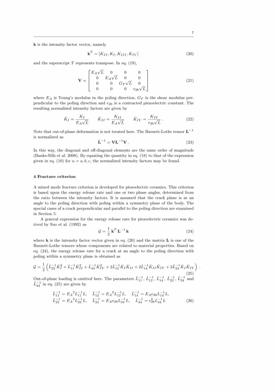
k is the intensity factor vector, namely

kT = [KII ,KI ,KIII ,KIV ] (20)

and the superscript T represents transpose. In eq. (19),

V =

EA

√L 0 0 0

0 EA

√L 0 0

0 0 GT

√L 0

0 0 0 e26√L

(21)

where EA is Young’s modulus in the poling direction, GT is the shear modulus per-

pendicular to the poling direction and e26 is a contracted piezoelectric constant. The

resulting normalized intensity factors are given by

KI =KI

EA

√L

KII =KII

EA

√L

KIV =KIV

e26√L. (22)

Note that out-of-plane deformation is not treated here. The Barnett-Lothe tensor L−1

is normalized as

L−1 = VL−1V . (23)

In this way, the diagonal and off-diagonal elements are the same order of magnitude

(Banks-Sills et al. 2008). By equating the quantity in eq. (18) to that of the expression

given in eq. (10) for α = a, b, c, the normalized intensity factors may be found.

4 Fracture criterion

A mixed mode fracture criterion is developed for piezoelectric ceramics. This criterion

is based upon the energy release rate and one or two phase angles, determined from

the ratio between the intensity factors. It is assumed that the crack plane is at an

angle to the poling direction with poling within a symmetry plane of the body. The

special cases of a crack perpendicular and parallel to the poling direction are examined

in Section 5.

A general expression for the energy release rate for piezoelectric ceramics was de-

rived by Suo et al. (1992) as

G =1

2kT L−1 k (24)

where k is the intensity factor vector given in eq. (20) and the matrix L is one of the

Barnett-Lothe tensors whose components are related to material properties. Based on

eq. (24), the energy release rate for a crack at an angle to the poling direction with

poling within a symmetry plane is obtained as

G =1

2

(L−122 K

2I + L−1

11 K2II + L−1

44 K2IV + 2L−1

12 KIKII + 2L−114 KIIKIV + 2L−1

24 KIKIV

).

(25)

Out-of-plane loading is omitted here. The parameters L−111 , L−1

12 , L−114 , L−1

22 , L−124 and

L−144 in eq. (25) are given by

L−111 = EA

2L−111 L, L−1

12 = EA2L−1

12 L, L−114 = EAe26L

−114 L,

L−122 = EA

2L−122 L, L−1

24 = EAe26L−124 L, L−1

44 = e226L−144 L (26)

8

where L−1ij are elements of the matrix L−1, EA and e26 are the Young’s modulus in

the poling direction and a piezoelectric coupling coefficient, respectively, and L is a

characteristic length of the problem. The relation between the matrices L−1

and L−1

is given in eq. (23). It is worth mentioning that the units of L−1ij are N/m. Finally, the

intensity factors in eq. (25) are normalized according to eqs. (22).

The energy release rate G may be rewritten as

G =1

2L−122 K

2I

(1 + 2

L−124

L−122

KIV

KI

+ 2L−112

L−122

KII

KI

+ 2L−114

L−122

KIIKIV

K2I

+L−144

L−122

K2IV

K2I

+L−111

L−122

K2II

K2I

).

(27)

Thus, it is possible to define

GI ≡1

2L−122 K

2I . (28)

When the crack propagates G = Gc, so that

Gc = GIc

(1 + 2

L−124

L−122

KIV

KI

+ 2L−112

L−122

KII

KI

+ 2L−114

L−122

KIIKIV

K2I

+L−144

L−122

K2IV

K2I

+L−111

L−122

K2II

K2I

)(29)

where

GIc =1

2L−122 K

2Ic . (30)

To obtain GIc, values of GI from eq. (28) are obtained at failure for each test and

averaged, as will be discussed in the sequel. Introducing two phase angles

ψ = tan−1 KIV

KI

, ϕ = tan−1 KII

KI

(31)

eq. (29) becomes

Gc = GIc

(1 + 2

L−124

L−122

tanψ + 2L−112

L−122

tanϕ+ 2L−114

L−122

tanψ tanϕ+L−144

L−122

tan2 ψ +L−111

L−122

tan2 ϕ

).

(32)

This is a three-dimensional failure surface for the case in which the crack faces are at

an angle to the poling direction and in which the critical energy release rate Gc is a

function of the phase angles ψ and ϕ.

For a crack perpendicular to the poling direction, the component L−114 is zero.

In addition, for symmetric applied loading and electric field, KII was found to be

negligible, as will be shown in the sequel. Therefore, for this case, there is only one

non-zero phase angle ψ given in eq. (31)1 leading to the failure curve

Gc = GIc

(1 + 2

L−124

L−122

tanψ +L−144

L−122

tan2 ψ

). (33)

For a crack perpendicular to the poling direction, there is coupling between the first

and fourth modes of fracture. This coupling is expressed by the second term in the

parentheses of the right hand side of eq. (33).

For a crack parallel to the poling direction, L−124 is zero. In addition, in the four-point

bend specimen tested here, both the applied loading and electric field were symmetric,

9

P a

F/2 F/2

W

LS1

S2

Fig. 2 Four-point bend specimen.

so that KII was negligible (implying ϕ = 0) and there was nearly no coupling between

modes I and IV (see Section 5.2). Thus, the failure curve for a crack parallel to the

poling direction with symmetric applied loading and electric field may be found based

on eq. (32) as

Gc = GIc

(1 +

L−144

L−122

tan2 ψ

). (34)

5 Fracture tests and analysis

Fracture tests on poled and unpoled PZT-5H (Morgan Electro Ceramics, Wrexham,

UK) ceramics have been performed. Both electric fields and mechanical loads were

applied during the fracture tests. An Instron (Bucks, UK) loading machine No. 8872

was employed with a load cell of 250 N maximum capacity. The displacement rate of

the tests was set to 0.001 mm/sec; this rate was controlled using a ±2.5 mm LVDT,

which was connected to the loading machine. An electric potential was applied through

the electrodes of the specimen using a high dc power supply with a capacity of 5 kV.

A modular Navitar microscope with a 24 x zoom and directional front illumination

was employed to visualize an area near the upper surface of the specimen along its

centerline. Pictures of this area were taken every three seconds by a Pixelink PL-A686

high resolution microscopy camera, which is designed to capture quality images. This

camera has a resolution of 6.6 Megapixels.

Tests were carried out on four-point bend specimens illustrated in Fig. 2 according

to an ESIS standard (2000). The nominal dimensions of the specimens are width W =

4 mm, length L = 45 mm, thickness B = 3 mm, spans S1 = 40 mm and S2 = 20 mm

(see Figs. 2 and 3). The tests were conducted on a specimen with a centrally located

edge notch. The initial notch was created by a diamond saw blade. For the unpoled

specimens, the width of the diamond saw blade was 0.35 mm. In order to decrease

the width of the notch, a diamond saw blade with a width of 0.2 mm was used for

the poled specimens. It may be noted that this notch was machined twice in order to

10

L=45mm, W=4mm 0.2mm, B=3mm 0.2mm+_+_

LB

W

V-notch

(a)

ab

c

b

S

(b)

a = 0.8 - 1.2mm

b ~ 0.5mm

c > width of razor

a - b > c

b ~ 30 , or as small as possible

S = V-notch width

Ay

x

Fig. 3 Schematic view of geometry of (a) V-notch specimen and (b) notch detail.

LVDT

specimen

load cell

four-point bend jig

Fig. 4 Fracture specimen in four-point bend jig.

obtain symmetric corners at its edges. The second notch was created using a Techni

Edge knife. For poled specimens, the crack faces were parallel to the poling direction.

The four-point bend jig, which was fabricated for this application is shown in Fig. 4.

This apparatus was made of graphite epoxy G10, which is an insulating material and

was chosen in order to prevent sparks between the poled piezoelectric specimen and

the jig.

11

5.1 Fracture tests of unpoled material

Nine unpoled PZT-5H specimens were tested. The dimensions of the specimens and

the notches are presented in Table 9 in the Appendix. The notch dimensions were

measured using ANALYSIS (2006) software for image processing. It may be observed

from Table 9 that for all specimens, the second notch does not conform to the standard

(a − b > c), since the width of the initial notch c is larger than the length a − b (see

Fig. 3). There were some technical difficulties in creating the second notch and some

of the specimens broke during this process. The initial notch width c is almost two

times greater than the width of the diamond saw blade. In addition, for some of the

specimens, the total length of the notch was smaller than the standard requirement of

0.8 mm. This occurred for specimens F-7, F-8, F-9 and F-11. In addition, for some of

the specimens, the angle of the second notch β is larger than 30◦. It may be noted that

insertion of this angle is quite difficult to control.

For all specimens, except F-7 and F-11, an area near the upper surface surrounding

the centerline of the specimen was photographed during the test. The vertical and

horizontal displacements of a point along the centerline of the specimen near its upper

side are obtained using ANALYSIS (2006) and LABVIEW (2007) softwares. The weight

of the upper part of the loading device (1.4 N) was taken into account in the load-

displacement curves. For the most part, the curves are nonlinear. For specimens F-7 and

F-11, the region near one of the rollers and not that of the centerline was photographed.

Digital analysis in this region did not provide smooth displacement data. Hence, graphs

for these two specimens were not produced. The horizontal displacement was smaller

by at least one order of magnitude than the vertical displacement for all specimens;

therefore, its influence was neglected.

The load at fracture Fc was measured at the end of each fracture test; the fracture

toughness was calculated according to this value for each specimen. For crack lengths

0.8 mm ≤ a ≤ 1.2 mm, values of KIc were calculated using the relation

KIc =Fc

B√W

S1 − S2W

3√α

2 (1− α)1.5Y (35)

where B and W are the specimen thickness and width (see Fig. 3a), S1 and S2 are the

support spans (see Fig. 2), α = a/W and Y is the stress intensity calibration factor

given by

Y = 1.9887− 1.326α−(3.49− 0.68α+ 1.35α2

)α (1− α)

(1 + α)2. (36)

For the specimens with a notch depth less than 0.8 mm, the calculation of KIc was

carried out using a finite element analysis, since it could not have been calculated

according to eq. (35). These analyses were performed on normalized notch lengths of

α = 0.175, 0.1875 and 0.2; the fracture toughness was calculated by linear interpolation

for notch lengths in that range. It may be noted that the difference between the value

calculated from the finite element analysis and eq. (35) for α = 0.2 was 0.5%.

Values of the load at fracture and the fracture toughness are presented in Table 1.

Specimens F-2 and F-15 were broken at loads of 20.3 and 8.4 N, respectively, which

are much smaller than the values obtained for the rest of the specimens. For these

specimens fracture did not occur in a straight line ahead of the notch, but rather at

an angle to this line. It was concluded that there were some initial cracks in these

12

Table 1 Load at fracture, fracture toughness and reduced Young’s modulus for tests of un-poled PZT-5H.

specimen no. a (mm) Fc (N) KIc (MPa√m) E (GPa)

F-2 0.84 20.3 - -

F-7 0.72 31.6 0.98 33.6

F-8 0.71 33.1 1.00 34.0

F-9 0.71 35.0 1.08 31.5

F-10 0.80 34.1 1.13 24.4

F-11 0.75 31.4 0.99 27.2

F-12 0.89 31.2 1.08 34.2

F-14 0.85 27.2 0.93 27.9

F-15 0.94 8.4 - -

specimens, probably created during the machining of the second notch. Therefore,

the fracture toughness was not calculated for these specimens. For all other specimens,

fracture occurred in a straight line ahead of the notch. The average value of the fracture

toughness for the unpoled material is KIc = 1.03 MPa√m.

Finally, the critical energy release rate may be calculated for the unpoled PZT-5H

material, which is isotropic. For plane strain conditions (Irwin 1958)

GIc =1− ν2

EK2

Ic (37)

where KIc is the fracture toughness, E is Young’s modulus and ν is Poisson’s ratio.

Here, KIc = 1.03 MPa√m and ν = 0.33 (Zhu and Yang 2004). It may be noted that

Young’s modulus was measured from tensile tests carried out on unpoled PZT-5H mate-

rial as E = 47.7 GPa (Motola et al. 2009). Use of this value in a finite element analysis,

carried out on specimen F-9, showed a different value for the vertical displacement at

point A (see Fig. 3a) than that obtained in the experiment through image processing. It

is assumed that this difference is a result of the nonlinear behavior of the piezoelectric

ceramic. The finite element analyses were carried out using a linear model. To account

for the nonlinearity of the piezoceramic in the finite element analysis, Young’s mod-

ulus E was reduced. This is a pseudo Young’s modulus which allows fitting between

the load-displacement curve found in the finite element analysis and in the experiment;

these values are presented in Table 1. The average value of Young’s modulus calculated

from Table 1 is E = 31.3 GPa; this value is smaller by 34% than that measured in the

tensile tests. The critical energy release rate for the unpoled material is obtained from

eq. (37) for each specimen and averaged to obtain GIc = 30.6 N/m.

5.2 Fracture tests of poled material

Sixteen poled PZT-5H specimens were tested. Both electric fields and mechanical loads

were applied during the fracture tests. The specimens were first poled with electrodes

attached at the specimen ends by Morgan Electro Ceramics (Wrexham, UK) and the

notches were machined parallel to the poling direction (see Fig. 2) at Tel Aviv Uni-

versity. An electric potential was applied through the electrodes of the specimen using

13

(a) (b)

Fig. 5 Poled PZT-5H four-point bend specimen with (a) electrodes placed at its edges and(b) conductive copper strips near the notch.

a high dc power supply with a capacity of 5 kV. One electrode was grounded and a

positive electric potential was applied on the other one. Initially, the potential differ-

ence was applied to the electrodes placed at the edges of the specimen, as illustrated in

Fig. 5a. At a later stage of the testing, conductive copper strips glued to the specimen

were used as electrodes; the distance between the two strips was 6 mm (see Fig. 5b).

Recall that for the former case the distance between the electrodes was 45 mm. The

specimen thickness B = 3 mm and its width W = 4 mm (see Fig. 3a); these are

nominal dimensions. By moving the electrodes closer together, a substantially lower

electric potential may be applied for a specific electric field. Specimens P-1, P-5, P-7,

P-10, P-25, P-26, P-38 and P-42 were tested with application of an electric potential

to the conductive strips; for the remainder of the specimens, an electric potential was

applied to the electrodes at the edges of the specimen. The absolute values of the

electric field applied in the experiments ranged between zero and 0.4 MV/m. In the

experiments, an electric field was applied, held at a given value, and then the specimen

was mechanically loaded until fracture occurred.

The dimensions of the specimens and the notches are presented in Table 10 in the

Appendix. A load-displacement curve was obtained for each specimen. Values of the

displacement were obtained using ANALYSIS (2006) and LABVIEW (2007) softwares.

The maximum vertical displacement, the load at fracture and the applied electric field

in each test are presented in Table 11 in the Appendix. The weight of the upper part of

the loading device (1.4 N) was taken into account in obtaining the load-displacement

curves. The average value of the load at fracture for the poled material is 31.0 N with

a range between 25.0 N and 38.4 N. Nonlinear behavior was found for all specimens.

A finite element analysis was carried out for each test using ANSYS (2007). A

model was made of a piezoelectric specimen containing a notch filled with an isotropic

dielectric material. The mesh in the vicinity of the notch for specimen P-10 is illustrated

in Fig. 6; the remainder of the mesh contained quadrilateral elements. This mesh

consists of 18,200 eight noded isoparametric elements and 55,261 nodal points. Meshes

for other specimens were similar to that in Fig. 6. The load at fracture Fc and electric

field E were applied in the analyses (see Table 11 in the Appendix). Electrodes were

placed at two alternative positions (see Fig. 5). For that in Fig. 5a, a suitable electric

potential was applied at the specimen edges. For the case shown in Fig. 5b, the electric

potential was applied at nodal points in the interior of the specimen along two lines

in the x-direction (see Fig. 3a) at a distance of 3 mm on each side of the specimen

centerline. On one line the applied electric potential was zero and on the other one

it had a positive value. The dimensions of the specimens and notches are given in

Table 10. It may be noted that it was not possible to model the radius of curvature of

the notch (S in Table 10) in the finite element model; therefore, the notch tip had a V-

shape. The angle of the V-shape notch β (see Table 10) changes for each finite element

analysis. In the finite element analysis, the thickness B = 1 m, whereas, its actual

14

notch

(b)(a)

notch

Fig. 6 (a) Mesh in the vicinity of the notch for specimen P-10 and (b) an enlargement of thearea surrounding the notch tip.

Table 2 Material properties for PZT-5H from Berlincourt and Krueger (1959).

property CE11 (GPa) CE

22 (GPa) CE55 (GPa) CE

12 (GPa) CE23 (GPa)

value 117 126 23.0 84.1 79.5property e11 (C/m2) e12 (C/m2) e26 (C/m2) κϵ11 (F/m) κϵ22 (F/m)value 23.3 -6.55 17.0 1.30095× 10−8 1.5045× 10−8

dimension is that given in Table 10. In the analyses, the applied load was adjusted

accordingly. Material properties of the piezoelectric specimen are those presented in

Table 2; however, some of these properties were changed, as will be discussed in the

sequel.

It was proposed to determine the dielectric permittivity within the notch by means

of a hybrid numerical/experimental method. To this end, an assumed value of the

permittivity was taken in the finite element analysis and the vertical displacement

of point A (see Fig 3a) along the centerline of the specimen near its upper side was

found. This value was compared to that measured in the experiment by means of image

processing. If these values were equal, then the dielectric permittivity of the media

inside the notch was to be taken as that in the finite element model. If these values

were not equal, a new value of permittivity would be assumed in the finite element

model, until convergence was attained. However, it was found that the permittivity

has a negligible influence on the finite element results. Values of κa = 0, κ0, 2κ0, 5κ0and 10κ0 were taken in the analyses of specimens P-9 and P-12 and the same value

of the vertical displacement of point A was obtained in all models. Therefore, for all

subsequent analyses, it was assumed that since the notches are quite wide, the value

of the dielectric permittivity inside them is that of air, namely κa = κ0.

Initially, material properties of PZT-5H given in Table 2 were used for the specimen

in the finite element model. However, the vertical displacement obtained in the finite

element model was much lower than the value measured in the experiment. It may

be mentioned that the mechanical properties were measured by a resonance technique

by the manufacturer and may be found as EA = 48.8 GPa and ET = 60 GPa from

15

the data in Table 2. Note that the axial and transverse directions are in the x and

y-directions (see Fig. 3a), respectively. Young’s modulus ET was measured by Motola

et al. (2009) by means of tensile tests. This property was determined as ET = 50.3 GPa

for an electric field E = 0, which is 16% lower than that given by the manufacturer.

The manufacturer used resonance tests to determine the mechanical properties; it was

seen by Fett and Munz (2000) that resonance tests produce higher values for these

parameters than mechanical tests. Moreover, it was found by Fett et al. (2003) that

ET is not affected when the electric field is changed.

In the finite element analysis of specimen P-28, which had no notch and was es-

pecially tested in four-point bending for calibration of the material properties, both

EA and ET were taken as EA = 40.3 GPa and ET = 50.3 GPa, which are lower by

16% and 17%, respectively, from the values given by the manufacturer. It was seen

that even with this reduction in the mechanical properties, the correct displacement

at point A (see Fig. 3a) was not obtained in the finite element analysis and was lower

by 44% than that measured by image processing in the experiment. Therefore, it is

assumed that this difference is a result of the nonlinear behavior of the piezoelectric

ceramic. The finite element analyses were carried out using a linear model. To account

for the nonlinearity of the piezoceramic in the finite element analysis of P-28, Young’s

modulus in the transverse direction ET and the piezoelectric coupling coefficients e11and e12 were reduced. Bending is most influenced by these material properties. It was

found that the influence of other mechanical and piezoelectric properties on the vertical

displacement is negligible. The dielectric properties have no effect on bending and are

those given in Table 2 (namely κϵ11 and κϵ22 ). Recall that for PZT-5H, e11 = 23.3 C/m2

and e12 = −6.55 C/m2 (see Table 2). The correct vertical displacement for P-28 was

obtained with EA = 40.3 GPa, ET = 29 GPa, e11 = 7.77 C/m2 and e12 = −2.18 C/m2.

Material properties were calibrated according to the behavior of the load-displace-

ment curve for each specimen. That is, finite element analyses were carried out iter-

atively until the numerically obtained load-displacement curve agreed approximately

with that obtained experimentally. These calibrated material properties for the four-

point bend specimens given in Table 12 in the Appendix may be compared to EA =

48.8 GPa and ET = 60 GPa obtained from the material properties in Table 2 which

are given by the manufacturer (Berlincourt and Krueger 1958), ET = 50.3 GPa as de-

termined by Motola et al. (2009) by means of tensile tests, and e11 and e12 presented

in Table 2. It may be observed in Table 12 that for all specimens the reduced values

of EA, e11 and e12 are the same. For specimens P-5, P-9, P-12, P-16, P-17, P-18 and

P-38, as well as for specimens P-1, P-7 and P-13, the reduced value of ET is the same.

Whereas for the remainder of the specimens the value of ET differs for each one. For all

specimens, EA and ET are reduced by 17% and approximately 50%, respectively, and

the piezoelectric coupling coefficients are smaller by about one third than those given

in Table 2. These material parameters should not be considered as the actual material

parameters but rather those that account for the nonlinear behavior of the material. It

may be noted that the finite element analyses of specimens P-9 and P-12 with different

values of dielectric permittivity inside the notch were carried out with the reduced

mechanical and piezoelectric properties given in Table 12. It was found once again that

different values of κa/κ0, between zero and 10, do not affect the vertical displacement

of point A shown in Fig. 3a.

The load-displacement curves obtained from the experiment and the finite element

analysis for specimens P-10 and P-47 are shown in Fig. 7. It may be observed in this

figure that the load-displacement curve is nonlinear for both specimens. However, the

16

30

20

10

0 0.02 0.04 0.06(b)

experimentFE

(a)

30

20

10

0 0.02 0.04 0.06

A

x

yP

ux(mm)

F(N

)

ux(mm)

F(N

)

Fig. 7 Experimental and numerical load-displacement curves at point A in the x-directionfor specimens (a) P-10 and (b) P-47.

2

1

2

1

1

2

12 1 2

Fig. 8 Integration paths for the notch in the poled PZT-5H specimen.

nonlinearity is greater for specimen P-10 in Fig. 7a than for specimen P-47 in Fig. 7b;

for specimen P-10, the applied electric field was twice that as for P-47. Hence, it

appears logical that the nonlinearity is greater for specimen P-10. The solid line in

Fig. 7, which represents the finite element analysis (FE), goes through zero and fits the

experimental points near the load at fracture. Similar nonlinear behavior was observed

for other specimens.

Intensity factors were calculated for each test using the M -integral. In the finite

element analysis, the notch was filled with a dielectric material. From the results, the

displacements un and the electric potential ϕ on the notch faces were calculated and

substituted into eqs. (8) and (9) to obtain the energetically consistent boundary con-

ditions on the notch faces. The M -integral was evaluated along two paths surrounding

the notch tip, as illustrated in Fig. 8. Recall that theM -integral for a notch with appli-

cation of the energetically consistent boundary conditions consists of an area integral

and line integrals, as described in eq. (10) and Fig. 1. Nevertheless, here, the notch

tip is not curved as in Fig. 1b and is V-shaped. The front edge of the notch including

the V and the two horizontal lines of its wider part in Fig. 8 were not included in the

calculation. It was found that values of the line integrals in eq. (10) were smaller by

four to five orders of magnitude than the area integral. Hence, the integral along these

lines was excluded from the calculation. Thus, the two paths of theM -integral included

17

Table 3 Average values of KI and KIV obtained with the M -integral for the four-point bend

PZT-5H poled specimens.

specimen a (mm) Fc (N) E (MV/m) KI × 10−5 KIV × 10−5

P-5 0.82 34.0 0.4 2.91 3.09

P-25 0.76 29.5 0.3 2.42 2.22

P-42 0.80 38.4 0.3 3.28 2.27

P-10 0.78 32.3 0.2 2.69 1.51

P-9 0.67 30.0 0.1 2.41 0.769

P-12 0.81 31.7 0.1 2.74 0.817

P-26 0.84 30.6 0.1 2.61 0.776

P-13 0.88 30.7 0 2.72 O(10−12)

P-18 0.87 25.0 0 2.25 O(10−11)

P-16 0.94 32.3 -0.1 3.02 -0.884

P-17 0.72 31.5 -0.1 2.47 -0.763

P-47 0.87 30.0 -0.1 2.67 -0.848

P-49 0.81 25.9 -0.1 2.18 -0.808

P-7 0.81 32.3 -0.2 2.69 -1.53

P-38 0.80 29.5 -0.3 2.39 -2.29

P-1 0.82 32.5 -0.4 2.77 -3.10

the elements shown in Fig. 8 and the straight lines, which are paths C2, C4, C6 and C7

in eq. (10) and Fig. 1a. It may be seen in Fig. 8 that the elements within these paths

are taken far from the notch tip; hence, its influence on the calculation is minimized.

It may be further pointed out that the radius of curvature of the notch S in the tested

specimens given in Table 10 is relatively small in comparison to the total notch length

a (the maximum value of S is 40 µm). Therefore, the ratio of S/a approaches zero in

the finite element models and the notch is sufficiently narrow, so that it may be treated

as a crack in relating the stress intensity factors to the M -integral in eq. (18).

Values of KI and KIV , given in eq. (22)1 and (22)3 were obtained from the two

paths using the M -integral (see Fig. 8); the average from these two paths is presented

in Table 3. Normalization of the intensity factors in eq. (22) is carried out using EA =

40.3 GPa (see Table 12), e26 = 17 C/m2 (see Table 2) and L = 1 m (L = B, the

thickness in the finite element analysis). Values of KII were negligible in comparison

to the other intensity factors; therefore, these values are not presented. The stress

intensity factor KII was between O(10−7) to O(10−9) for cases in which an electric

field was applied and O(10−16) to O(10−17) when only a mechanical load was applied;

hence, it was assumed to be zero. First, path independence was examined. It was

observed that values of KI agreed to 2 significant figures for the two paths. For KIV ,

values along the two paths agreed to 2 significant figures when KIV is O(10−5). For

lower absolute values of KIV , poorer agreement between paths was found.

It may be observed in Table 3 that KI is strongly influenced by the mechanical

force. The influence of the electric field on KI appears to be negligible. On the other

hand, the electric field highly influences KIV , as may be seen in Table 3. Its value

changes approximately according to the change in the electric field. For example, when

18

-0.5 -0.4 -0.3 -0.2 -0.1 0 0.50.40.30.20.1

-0.5 -0.4 -0.3 -0.2 -0.1 0 0.50.40.30.20.1

-1

-2

-3

-4

1

2

3

4

(a) (b)

0.5

1.0

1.5

2.5

2.0

3.0KI^

E (MV/m)

E (MV/m)

KIV^

3.5 x10-5

x10-5

Fig. 9 The normalized intensity factors (a) KI and (b) KIV versus the applied electric fieldin the four-point bend experiments.

E = 0.4 MV/m, KIV is almost four times higher than the value obtained for E =

0.1 MV/m. Furthermore, when E = 0, values of KIV are O(10−16) and O(10−17),

which are taken as zero. In addition, the sign of the electric flux density intensity

factor is determined by the sign of the electric field and its behavior is relatively

symmetric. Nevertheless, it appears that the mechanical force also affects KIV . For

a specific electric field, an increase of the load at fracture is generally followed by an

increase in the absolute value of KIV .

A further analysis was carried out for specimen P-1 with application of the imper-

meable boundary conditions. Hence, the dielectric permittivity inside the notch was

taken as zero, so that the notch was no longer filled with a dielectric material. It was

found that KIV differed by 0.1% with respect to the results obtained for the ener-

getically consistent boundary conditions. The difference between values of KI for the

impermeable and exact boundary conditions was negligible. In addition, another anal-

ysis with the dielectric permittivity inside the notch κa = 10κ0 was carried out for

specimen P-42. It should be noted that the line integrals along the notch faces were

included in the calculations. The difference between KI for the energetically consistent

boundary conditions with κa = κ0 and κa = 10κ0 was negligible, as well. On the

other hand, KIV differed by -0.8% with respect to the results obtained for the ener-

getically consistent boundary conditions with application of κa = κ0. An analysis with

application of the impermeable boundary conditions slightly increased the electric flux

density intensity factor in comparison to an analysis with the energetically consistent

boundary conditions and κa = κ0. Whereas, an analysis with κa = 10κ0 decreased

KIV . Values of KI were not influenced by the permittivity, as observed in Motola and

Banks-Sills (2009).

In Fig. 9, graphs of the normalized intensity factors KI and KIV from eqs. (22)1and (22)3 versus the applied electric field are presented. The normalized stress intensity

factor KI is plotted in Fig. 9a and approximated by a least square straight line parallel

to the horizontal axis. From this graph, the value of KIc = 2.64× 10−5 is obtained. A

value of KIc may be calculated from KIc by means of eq. (22)1 as KIc = 1.06 MPa√m.

19

Table 4 Material properties for PIC-151 (Jelitto et al. 2005b).

property CE11 (GPa) CE

22 (GPa) CE55 (GPa) CE

12 (GPa) CE23 (GPa)

value 100.45 107.65 19.624 63.854 63.124property e11 (C/m2) e12 (C/m2) e26 (C/m2) κϵ11 (F/m) κϵ22 (F/m)value 15.1 -9.6 12.0 7.5402× 10−9 9.8235× 10−9

In eq. (22)1, EA = 40.3 GPa (see Table 12) and the characteristic length L = 1 m (L =

B, the thickness in the finite element analysis). It should be emphasized that KIc is the

apparent fracture toughness for mixed mode, which should not be used for predicting

failure, but only for obtaining the failure curve. Recall that for the unpoled material,

the average value of the fracture toughness was obtained as KIc = 1.03 MPa√m (see

Section 4.1). Of course, for the poled material failure is more complicated involving

mixed modes. For the unpoled material, there is a single mode of fracture; thus, KIc

may be used to predict failure for this case. For PZT-5H, the difference in values of KIc

between the unpoled and the material poled parallel to the crack faces is negligible.

Next, the electric flux density intensity factor KIV is plotted in Fig. 9b. It behaves

linearly with respect to the applied electric field E and may be approximated by

KIV = 7.68× 10−5E (38)

where the regression coefficient R2 = 0.999.

To conclude, for this case in which the crack faces are parallel to the poling direction,

there appears to be nearly insignificant coupling between the first and fourth modes

of fracture. The decoupling was observed in the finite element analyses. Values of KI

were only affected by the applied force, whereas, KIV was influenced mainly by the

electric field. For a crack parallel to the poling direction, coupling exists between KII

and KIV . For this poling direction, both KII and KIV cause in-plane notch sliding

displacement. However, in these experiments KII was negligible.

5.3 Analysis of experimental results from Jelitto et al. (2005b)

Tests were carried out by Jelitto et al. (2005b) on four-point bend specimens fabri-

cated from the piezoelectric ceramic PIC-151. This material is similar to PZT-5H. In

these experiments the crack faces were perpendicular to the poling direction and both

mechanical loads and electric fields were applied. Material properties are taken from

Jelitto et al. (2005b) and are presented in Table 4, for the poling direction along the

x1-axis (the −y-axis in Fig. 10). Following Jelitto et al. (2005b), the dimensions of the

specimens are L = 24 mm, S1 = 20 mm, S2 = 10 mm, the width W = 4 mm and

the thickness B = 3 mm (see Fig. 10). The samples were placed in a Fluorinert-liquid

to prevent electric sparks; this material is dielectrically isotropic with the permittivity

κa = 1.75κ0.

Using the same boundary conditions applied in the tests by Jelitto et al. (2005b),

numerical analyses were carried. In the finite element analyses, the thickness B = 1 m,

whereas its actual dimension was 3 mm. Initially, analyses were carried out by modeling

the notch as a crack, as described in Motola and Banks-Sills (2009); in prescribing

the energetically consistent boundary conditions in eqs. (8) and (9), iterations are

20

F/2 F/2

a

S2S1

L

WPx

y

aR

Fig. 10 Four-point bend specimen and an enlargement of the notch for analyses of experi-mental results of Jelitto et al. (2005b).

required. In this case, because of the low applied loads, convergence could not be

reached. Therefore, a specimen with a notch was analyzed instead. According to the

specimen configurations, several notch lengths were used in the analyses, namely a =

1.1 mm, 1.5 mm and 2.0 mm; the notch radius R = 90 µm (see Fig. 10). The ratio of

R/a ranged between 0.045 and 0.082; hence, it was sufficiently small, so that the notch

may be treated as a crack in using eq. (18) and as described in Section 3.

First, two finite element models were analyzed. The first model contained a piezo-

electric specimen with a notch filled with dielectric isotropic material (Fluorinert-

liquid); whereas the second one consisted of an empty notch within the specimen.

For the second model, the analyses were conducted by means of an iterative procedure

for which the normal electric flux density Dn and stress σnn were calculated at each

step from the normal displacement and electric potential values using eqs. (8) and (9).

For the first iteration, impermeable boundary conditions were enforced, so that the val-

ues of the normal electric flux density and stress on the notch surfaces were zero. The

analyses of the two models were carried out for crack length a = 2 mm, applied electric

field E = 0.45 MV/m and load at fracture Fc = 7367 N (for the actual thickness of the

specimen of 3 mm the equivalent force is 22.1 N). The finite element meshes contained

78,100 and 75,700 eight noded isoparametric elements and 235,651 and 228,594 nodal

points for the model with the filled and empty notch, respectively. The meshes in the

vicinity of the notch tip were similar for both models and are shown in Fig. 11.

The M -integral was evaluated along two paths surrounding the notch tip. Recall

that the M -integral for a notch with application of the energetically consistent bound-

ary conditions consists of an area integral and line integrals (see eq. (10)). To minimize

the influence of the notch tip, the elements on the integration paths were taken far

from the notch tip. Values of the average normalized intensity factors, obtained from

the two paths, with application of Fc = 7367 N and E = 0.45 MV/m for a = 2 mm,

are presented in Table 5 for both models. Recall the normalization in eqs. (22). Fifty

iterations were carried out for the analysis with the empty notch with a maximum

tolerance of 0.01% for the electric flux density and the stress on the crack faces in

eqs. (8) and (9). Note that the line integrals along the notch boundary were negligible

in the calculation and differed by less than 3%. Moreover, it may be observed in Table 5

that the difference between results for the two models with the filled and empty notch

is -1.5% and 1.4% for KI and KIV , respectively. Values of the normalized intensity

21

notchnotch

(a) (b)

Fig. 11 Mesh in the vicinity of the notch for (a) the filled notch and (b) the empty notch.

Table 5 Average normalized values of the intensity factors for a = 2 mm, E = 0.45 MV/mand F = 7367 N for a four-point bend specimen of Jelitto et al. (2005b) shown in Fig. 10 witha filled and empty notch.

KI × 10−5 KII KIV × 10−5

filled notch 1.34 O(10−13) 6.96empty notch 1.36 O(10−14) 6.86

factor KII were negligible for both models. It may be pointed out that analyses of the

model with the empty notch, which were based on iterations, required computer time

which was two orders of magnitude greater than that for the filled notch. Furthermore,

the model with the filled notch is considered more accurate, since the iterative model

is based on approximate equations (eqs. (8) and (9)). Therefore, the remainder of the

analyses were carried out only on the model with the filled notch. A coarse mesh was

designed for the model with the filled notch consisting of 18,750 elements and 56,841

nodal points. The differences between the fine and coarse meshes were -4.1% and -

.2% for KI and KIV , respectively. Hence, for all results presented in this section, fine

meshes were employed.

Different loads and electric fields were applied in the finite element analyses of each

specimen as shown in Table 6. Note that the applied force in Table 6 is adjusted to the

3 mm thickness. The finite element meshes contained between 68,020 and 80,480 eight

noded isoparametric elements and 205,373 and 242,799 nodal points depending upon

notch length. The mesh in the vicinity of the notch edge is illustrated in Fig. 11a for

a = 2 mm; the remainder of the mesh not shown contained quadrilateral elements.

Average values of KI and KIV , given in eqs. (22)1 and (22)3, respectively, and

obtained from two paths, with application of different loads and electric fields for all

notch lengths, are presented in Table 6. In eqs. (22), EA = 60.2 GPa, as calculated

according to material properties given in Table 4, and e26 = 12.0 C/m2 (see Table 4).

Values of KII were negligible in comparison to the other intensity factors; therefore,

these values are not presented. The stress intensity factor KII was O(10−8) for a =

22

Table 6 Average values of KI and KIV obtained with the M -integral for the four-point bend

specimen of Jelitto et al. (2005b) in Fig. 10 with application of different loads and electric

fields for all notch lengths.

a (mm) Fc (N) E (MV/m) KI × 10−5 KIV × 10−5

2 22.1 0.45 1.35 6.81

2 22.5 0.30 1.41 5.41

2 23.6 0.15 1.48 4.00

2 23.6 0 1.48 2.48

2 22.0 -0.30 1.39 -0.730

2 21.4 -0.45 1.35 -2.31

2 22.4 -0.60 1.41 -3.73

1.5 36.3 0.30 1.62 5.32

1.5 34.7 0 1.54 2.60

1.5 33.2 -0.30 1.47 -0.115

1.5 33.3 -0.45 1.48 -1.41

1.5 32.6 -0.60 1.45 -2.76

1.5 35.9 -0.75 1.59 -3.82

1.1 37.6 0.60 1.29 6.59

1.1 40.5 0.45 1.39 5.65

1.1 41.3 0.30 1.41 4.58

1.1 42.9 0 1.46 2.47

1.1 42.1 -0.15 1.44 1.32

1.1 39.2 -0.30 1.34 0.0497

1.1 mm and a = 1.5 mm and O(10−13) to O(10−14) for a = 2 mm; hence, it was

assumed to be zero. It is observed in Table 6 that the influence of the electric field on

KI is negligible and the effect of the applied load predominates. For a specific crack

length, KI is approximately proportional to the critical applied load Fc. On the other

hand, both the mechanical force and electric field affect values of KIV (see Table 6).

The greater the value of the electric field, the greater the value of KIV . Furthermore,

for E = −0.3 MV/m and a = 1.1 and 1.5 mm, KIV differs by 1-2 orders of magnitude

from its value obtained for E = 0.3 MV/m. Path independence was examined, as well.

It was seen that for KI there were slight differences if at all between the two paths. For

KIV , paths agreed to 2 to 3 significant figures when KIV was of order O(10−5). For

lower absolute values of KIV , poorer agreement between paths was found. Nevertheless,

when KIV is of order O(10−7), it may be considered as zero.

Values of KIV are plotted versus those of KI and presented in Fig. 12. It is observed

that values of KI are relatively constant with respect to KIV . The average value of KI ,

obtained for all points, is 1.44 × 10−5. Note that Jelitto et al. (2005b) calculated the

intensity factors for impermeable and permeable boundary conditions using the stress

extrapolation method. The average value of KI was approximately 0.9 MPa√m for

both boundary conditions. Whereas, values of KIV ranged between −0.5 × 10−3 and

1.0×10−3 C/m3/2 for the impermeable boundary conditions and between 0.25×10−3

and 0.32× 10−3 C/m3/2 for the permeable boundary conditions. In this investigation,

23

6

4

2

0

-2

-4

x10-5

KIV^ KI(average)=1.44x10-5^

a=2mma=1.5mma=1.1mm

0.5 1.51KI^

x10-5

8

2

-6

Fig. 12 The intensity factor KIV versus KI from analyses of experimental results of Jelittoet al. 2005b.

the average value of the mode I stress intensity factor KI = 0.86 MPa√m and KIV

ranges between −0.46× 10−3 and 0.82× 10−3 C/m3/2.

A further analysis was carried out for a = 2 mm, E = 0.45 MV/m and Fc = 22.1 N

with application of the impermeable boundary conditions. Hence, the dielectric per-

mittivity inside the notch was taken as zero, so that the notch was no longer filled with

a dielectric material. It was found that KI and KIV differed by 3.2% and 2.2%, respec-

tively, with respect to the results obtained for the energetically consistent boundary

conditions. Thus, in this case, an analysis with application of the impermeable bound-

ary conditions slightly overestimated these intensity factors.

5.4 Failure criterion

Fracture criteria obtained in Section 4 are applied using the intensity factors obtained

for the two cases considered here in which the crack faces are perpendicular and parallel

to the poling direction. First, the failure criterion in eq. (33) is applied using the

intensity factors presented in Table 6 for four-point bend PIC-151 specimens poled

perpendicular to the crack faces. For each test, the critical energy release rate Gc and

the phase angle ψ were calculated using eqs. (25) and (31)1, respectively, with the

intensity factors in Table 6 and with KII = 0. These values are presented in Table 7.

24

Table 7 Values of the critical energy release rate Gc, the phase angle ψ and the domainswitching zone size Rs obtained for fracture tests of Jelitto et al. (2005b).

specimen no. a (mm) Fc (N) E (MV/m) Gc (N/m) ψ Rs (mm)

J-1 2.0 22.1 0.45 0.0 1.38 0.62

J-2 2.0 22.5 0.30 6.0 1.32 0.39

J-3 2.0 23.6 0.15 10.3 1.22 0.21

J-4 2.0 23.6 0 11.4 1.03 0.08

J-5 2.0 22.0 -0.30 6.2 -0.48 0.01

J-6 2.0 21.4 -0.45 0.6 -1.04 0.07

J-7 2.0 22.4 -0.60 -5.6 -1.21 0.19

J-8 1.5 36.3 0.30 10.5 1.28 0.38

J-9 1.5 34.7 0 12.4 1.04 0.09

J-10 1.5 33.2 -0.30 8.6 -0.08 0.00

J-11 1.5 33.3 -0.45 5.1 -0.76 0.03

J-12 1.5 32.6 -0.60 -0.5 -1.09 0.10

J-13 1.5 35.9 -0.75 -4.9 -1.18 0.20

J-14 1.1 37.6 0.60 -0.3 1.38 0.58

J-15 1.1 40.5 0.45 4.9 1.33 0.43

J-16 1.1 41.3 0.30 8.0 1.27 0.28

J-17 1.1 42.9 0 11.1 1.04 0.08

J-18 1.1 42.1 -0.15 10.4 0.74 0.02

J-19 1.1 39.2 -0.30 7.4 0.04 0.00

It may be observed in Table 7 that some of the values of the critical energy release

rate are negative or close to zero; hence, these values are not physically plausible. It is

possible that this phenomenon occurs because of a large domain switching zone in the

vicinity of the notch tip. If the applied electric field or load is sufficiently high, it may

be anticipated that the domain switching zone near the notch tip becomes too large;

therefore, the small scale domain switching zone assumption justifying K-dominance

ceases to be valid. The size of the domain switching zone Rs may be estimated similarly

to the plastic zone near a crack tip for elastic materials and plane strain conditions

(Irwin 1960; Jelitto et al. 2005b) as

Rs =1

6π

(KIV

κ11Ec

)2

(39)

where Ec is the coercive field and is approximately 1.0 MV/m for PIC-151 (Schneider

2007) and κ11 is the permittivity in the poling direction (see Table 4). It may be noted

that the yield stress and KI in Irwin’s approach are replaced by the coercive field

multiplied by κ11 and KIV , respectively.

The size of the domain switching zone in the neighborhood of the notch tip was

calculated for each test according to eq. (39) and presented in Table 7. One would

like to assume that if the domain switching zone size is small with respect to the

25

5

0-0.5

a=2mma=1.5mma=1.1mm 10

15

0.5 1 1.5-1 y-1.5

gc(N/m)

Fig. 13 Fracture curve and experimental results of Jelitto et al. (2005b).

notch length and unbroken ligament, then the concept of K-dominance is valid. If on

the other hand, the zone is large with respect to in-plane dimensions, then the test

results must be analyzed by taking into account the nonlinear behavior. It may be

observed in Table 7 that Rs is large in comparison to the notch length for specimens

J-1, J-7, J-13 and J-14. In addition, for these specimens, the critical energy release

rate is zero or negative; therefore, on the basis of the large domain switching zone,

these specimens could be excluded in implementing the fracture criterion. It may be

noted that the size of the domain switching zone is not proportional to the value of Gc.One would expect that there should be such a correlation. Moreover, although positive

values of Gc are obtained for specimens J-2, J-3, J-8, J-15 and J-16, the length of the

domain switching zone is large in comparison to the notch length. Hence, the domain

switching zone criterion does not appear suitable for these tests. It may be further seen

in Table 7 that for specimens J-6 and J-12, in which negative electric fields are applied,

Rs is sufficiently small in comparison to the notch length, although the critical energy

release rate is close to zero. These points should also be excluded from the fracture

criterion. Note that higher values of KIV are obtained for positive electric fields (see

Table 6). Therefore, when a negative electric field is applied, it decreases the size of

the domain switching zone; whereas, application of a load and a positive electric field

increases its length. To conclude, the domain switching zone criterion presented here

does not appear suitable for these experiments and a modified criterion should be

developed.

In Fig. 13, a graph of the critical energy release rate Gc as a function of the phase

angle ψ is presented. It may be observed that Gc is not a constant, but rather a function

of the mode mixity. The colored symbols in Fig. 13 represent values of the critical energy

release rate calculated from eq. (25) vs ψ of eq. (31)1 for the fracture tests presented

in Table 7 with positive values of Gc; specimen J-6 is also excluded, although its value

is very close to the failure curve. In addition, eq. (33) is plotted as the solid curve in

Fig. 13. Values below this curve are safe; for those above it, failure is expected. The

value of GIc used for this curve is given in eq. (30). The value of KIc is found as the

average of the values of KI at failure in Table 6 excluding those for which Gc is negativeor close to zero. Its value is 1.46×10−5 which is slightly different from the value shown

in Fig. 12 which includes all of the tests. With L−122 = 8.151 × 1010 N/m a value of

GIc = 8.6 N/m is found. Excellent agreement is observed between the experimental

26

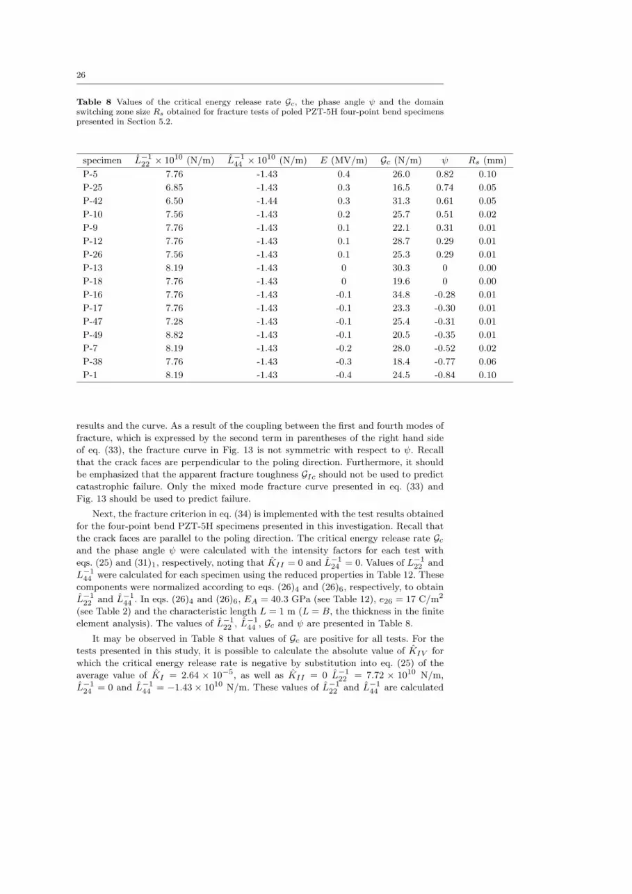
Table 8 Values of the critical energy release rate Gc, the phase angle ψ and the domainswitching zone size Rs obtained for fracture tests of poled PZT-5H four-point bend specimenspresented in Section 5.2.

specimen L−122 × 1010 (N/m) L−1

44 × 1010 (N/m) E (MV/m) Gc (N/m) ψ Rs (mm)

P-5 7.76 -1.43 0.4 26.0 0.82 0.10

P-25 6.85 -1.43 0.3 16.5 0.74 0.05

P-42 6.50 -1.44 0.3 31.3 0.61 0.05

P-10 7.56 -1.43 0.2 25.7 0.51 0.02

P-9 7.76 -1.43 0.1 22.1 0.31 0.01

P-12 7.76 -1.43 0.1 28.7 0.29 0.01

P-26 7.56 -1.43 0.1 25.3 0.29 0.01

P-13 8.19 -1.43 0 30.3 0 0.00

P-18 7.76 -1.43 0 19.6 0 0.00

P-16 7.76 -1.43 -0.1 34.8 -0.28 0.01

P-17 7.76 -1.43 -0.1 23.3 -0.30 0.01

P-47 7.28 -1.43 -0.1 25.4 -0.31 0.01

P-49 8.82 -1.43 -0.1 20.5 -0.35 0.01

P-7 8.19 -1.43 -0.2 28.0 -0.52 0.02

P-38 7.76 -1.43 -0.3 18.4 -0.77 0.06

P-1 8.19 -1.43 -0.4 24.5 -0.84 0.10

results and the curve. As a result of the coupling between the first and fourth modes of

fracture, which is expressed by the second term in parentheses of the right hand side

of eq. (33), the fracture curve in Fig. 13 is not symmetric with respect to ψ. Recall

that the crack faces are perpendicular to the poling direction. Furthermore, it should

be emphasized that the apparent fracture toughness GIc should not be used to predict

catastrophic failure. Only the mixed mode fracture curve presented in eq. (33) and

Fig. 13 should be used to predict failure.

Next, the fracture criterion in eq. (34) is implemented with the test results obtained

for the four-point bend PZT-5H specimens presented in this investigation. Recall that

the crack faces are parallel to the poling direction. The critical energy release rate Gcand the phase angle ψ were calculated with the intensity factors for each test with

eqs. (25) and (31)1, respectively, noting that KII = 0 and L−124 = 0. Values of L−1

22 and

L−144 were calculated for each specimen using the reduced properties in Table 12. These

components were normalized according to eqs. (26)4 and (26)6, respectively, to obtain

L−122 and L−1

44 . In eqs. (26)4 and (26)6, EA = 40.3 GPa (see Table 12), e26 = 17 C/m2

(see Table 2) and the characteristic length L = 1 m (L = B, the thickness in the finite

element analysis). The values of L−122 , L−1

44 , Gc and ψ are presented in Table 8.

It may be observed in Table 8 that values of Gc are positive for all tests. For the

tests presented in this study, it is possible to calculate the absolute value of KIV for

which the critical energy release rate is negative by substitution into eq. (25) of the

average value of KI = 2.64 × 10−5, as well as KII = 0 L−122 = 7.72 × 1010 N/m,

L−124 = 0 and L−1

44 = −1.43× 1010 N/m. These values of L−122 and L−1

44 are calculated

27

-1.5 -1.0 0 0.5 1.0 1.5y

10

20

30

-0.5

40gc (N/m)

P-49

P-17

P-47

P-13

P-16

P-5

P-18

P-12

P-26

P-9

P-42

P-10

P-25

P-7

P-1

P-38

E = -0.1 MV/mE = 0 E = -0.1 MV/mE = -0.2 MV/mE = -0.3 MV/mE = -0.4 MV/m

E = -0.4 MV/mE = -0.3 MV/mE = -0.2 MV/m

P a

F/2 F/2

W

Fig. 14 Fracture curve and experimental results of the four-point bend PZT-5H poled speci-mens (crack faces are parallel to the poling direction).

as the average of the values given in Table 8. Thus, a negative value of Gc is obtained

for |KIV | ≥ 6.13 × 10−5. If eq. (38) is extrapolated for values of |E| > 0.4 MV/m,

it is possible to calculate the value of the electric field E for which Gc is negative.

Substituting |KIV | = 6.13 × 10−5 into eq. (38) leads to E = 0.798 MV/m. Note that

this value is extremly close to the coercive field Ec ∼ 0.8 MV/m for PZT-5H (Schneider

2007).

The size of the domain switching zone Rs may be estimated similarly to that given

in eq. (39) as

Rs =1

6π

(KIV

κ22Ec

)2

(40)

where κ22 is the permittivity perpendicular to the poling direction (see Table 2).

The size of the domain switching zone was calculated for each test according to

eq. (40) and is presented in Table 8. In eq. (40), the coercive field Ec = 0.8 MV/m,

κ22 = 1.5045× 10−8 F/m (see Table 2) and values of KIV are calculated for each test

by means of eq. (22)3 using KIV given in Table 3, e26 in Table 2 and L = 1 m. It may

be observed in Table 8 that Rs is relatively small in comparison to the notch length for

all specimens, although the amount of domain switching increases with an increase in

the absolute value of the applied electric field. Thus, for the PZT-5H four-point bend

specimens in which the crack faces are parallel to the poling direction, the domain

switching effect is minor in comparison to the PIC-151 specimens for which the crack

faces are perpendicular to the poling direction.

In Fig. 14, the critical energy release rate Gc is plotted as a function of the phase

angle ψ given in eq. (31)1. The colored symbols in Fig. 14 represent the values of

the critical energy release rate and ψ for the each of the fracture tests presented in

Table 8. To obtain a plot of eq. (33), a value of GIc is required. This is obtained as

the average value of eq. (30) of each test, so that GIc = 27.0. Note that the average

value of the normalized mode I stress intensity factor at failure KIc is not used since

28

L−122 was taken to vary with each test. With this value of GIc, eq. (34) is plotted

as the solid curve in Fig. 14. It may be observed in Fig. 14 that with some scatter,

reasonable agreement is observed between the fracture curve and the experimental

results. Since there is decoupling between the electrical and mechanical loads, it would

be expected that the applied load would decrease with increase in crack length. It

may be observed in Table 11 that there is no correlation between applied load and

crack length. It is possible that the scatter is a result of a distribution in the damage

caused by introduction of the second notch (see Fig. 3) which is introduced manually.

Uniform dimensions of the notch between specimens were difficult to obtain. In fact,

the alignment of the two notches was less than perfect. Moreover, it was not possible

to conform to the restriction on the length of the second notch (a − b) in comparison

with the width of the first notch c (see Table 10). It is thought that the difficulty with

the second notch is the major source of the scatter. Improved tools for machining the

notch should enhance results in future research.

Finally, it may be recalled that GIc = 30.6 N/m for the PZT-5H unpoled material.

Since there was a single deformation mode for the unpoled material, there was a single

value for the fracture toughness or critical energy release rate GIc of this material.

On the other hand, for the poled material, GIc = 27.0 N/m is the apparent fracture

toughness and failure may not be predicted with this value. The value of GIc for

the unpoled material is higher than that obtained for the material (PZT-5H) poled

parallel to the crack faces. In addition, for PIC-151 poled perpendicular to the crack

faces GIc = 8.6 N/m. The material PIC-151 is similar to PZT-5H. Hence, it is seen that

material poled parallel to the crack faces is tougher than material poled perpendicular

to the crack faces. It is less tough than the unpoled material. It may be further noted

that in the analyses of the PIC-151 material poled perpendicular to the crack faces,

material properties were not reduced as for the poled PZT-5H in this investigation.

Thus, reduction in the material properties of PIC-151 poled perpendicular to the crack

faces may increase their GIc values.

6 Summary and Conclusions

This investigation included both numerical and experimental analyses carried out on

PZT four-point bend specimens. Fracture tests were conducted on unpoled and poled

PZT-5H four-point bend specimens. For the poled specimens, the crack (notch) faces

were parallel to the poling direction with both mechanical loads and electric fields

applied to the specimens. Finite element analyses were carried out on specimens with

notches using the conservativeM -integral; these analyses included crack face boundary

conditions. Experimental results of Jelitto et al. (2005b) were analyzed by means of

the conservative M -integral, as well. In that study, fracture tests were conducted on

four-point bend PIC-151 specimens with the notch faces perpendicular to the poling

direction. In addition, a general mixed mode fracture criterion was presented for piezo-

electric ceramics; this criterion was based upon the energy release rate and two phase

angles. The criterion was specialized for the two cases studied here.

The main observations from the numerical and experimental investigations are

summarized. From the analyses of the four-point bend poled PZT-5H specimens, it

was observed that the dielectric permittivity within the notch had negligible influence

on the results. It was assumed that since the notches were quite wide, the value of

the permittivity inside them was that of air, namely κa = κ0. For the four-point bend

29

PZT-5H specimens, the difference in values between the fracture toughness KIc of the

unpoled specimens and that of the apparent fracture toughness of the material poled

parallel to the crack faces was seen to be negligible. Material poled parallel to the

crack faces was found to be tougher (greater GIc) than material poled perpendicular

to the crack faces and less tough than the unpoled material. Excellent agreement was

observed between the fracture curve and the experimental results obtained for the

PIC-151 material poled perpendicular to the crack faces. Nevertheless, some values

of the critical energy release rate were negative or close to zero for this case. It was

assumed that these values were obtained because of the domain switching zone in the

vicinity of the crack tip. However, the domain switching zone criterion does not appear

suitable for these experiments and a modified criterion should be developed in the

future. Moreover, analyzing the specimens with the impermeable crack face boundary

conditions led to a difference of 3.2% and 2.2%, respectively, for the normalized intensity

factors KI and KIV . Recall that in this case the notch was filled with a fluid whose

dielectric permittivity was κa = 1.75κ0. Reasonable agreement was observed between

the fracture curve and the experimental results of the PZT-5H material poled parallel

to the crack faces. Here, the domain switching zone was not great, although the load

vs displacement curves from the tests were nonlinear.

Further investigation of the scatter in this case is required. It is also suggested that

in the future the fracture test be reanalyzed with a nonlinear constitutive relation. This

study presents a basis for a sound methodology for assessing failure of piezoelectric

ceramics.

Acknowledgements We would like to thank the Belfer family for their continuing support.In addition, we would like to express our appreciation to Dr. Hans Jelitto for providing us withdetails of experimental results performed by him and coworkers, as well as helpful communica-tions. We are indebted to Professor Raymond Boxman and Dr. Vladimir Weinstein for helpfuldiscussions and technical assistance related to electrical engineering aspects of the tests.

References

1. ANALYSIS (2006) Release 3.2, Olympus soft imaging systems, Munster, Germany2. ANSYS (2007) Release 11, Ansys, Inc., Canonsburg, Pennsylvania, U.S.A.3. Banks-Sills L, Sherman D (1992) On the computation of stress intensity factors for three-dimensional geometries by means of the stiffness derivative and J-integral methods. Int JFract 53:1–20

4. Banks-Sills L, Motola Y, Shemesh L (2008) The M-integral for calculating intensity factorsof an impermeable crack in a piezoelectric material. Engng Fract Mech 75:901-925

5. Berlincourt D, Krueger HA (1959) Properties of Morgan Electro Ceramic ceramics, Tech-nical Publication TP-226, Morgan Electro Ceramics

6. Bruce JG, Gerberich WW, Koepke BG (1978) Subcritical crack growth in PZT. In: BradtRC, Hasselman DPH, Lange FF (eds) Fracture mechanics of ceramics, crack growth andmicrostructure, Vol. 4, pp 687–709

7. Cao H, Evans AG (1994) Electric-field-induced fatigue crack growth in piezoelectrics. J AmCer Soc 77:1783–1786

8. Deeg WF (1980) The analysis of dislocation, crack and inclusion problems in piezoelectricsolids. Ph.D. thesis, Stanford University

9. ESIS Procedures and Documentations (2000) Procedure for determining the fracturetoughness of ceramics using the single-edge-V-notched beam (SEVNB) method. ESIS P5-00/VAMAS. European Structural Integrity Society

10. Fett T, Munz D (2000) Measurement of Young’s moduli for Lead Zirconate Titanate (PZT)ceramics. J Test Eval 28:27–35

30

11. Fett T, Munz D, Thun G (2003) Stress-strain behaviour of a soft PZT ceramic undertensile and compression loading and a transverse electric field. Ferroelec 297:83–90

12. Freiman SW, McKinney KR, Smith HL (1974) Slow crack growth in polycrystalline ce-ramics. In: Bradt RC, Hasselman DPH, Lange FF (eds) Fracture mechanics of ceramics,microstructure, materials, and applications, Vol. 2, pp 659–676

13. Fulton CC, Gao H (2001) Effect of local polarization switching on piezoelectric fracture.J Mech Phys Solids 49:927–952

14. Gao H, Zhang T-Y, Tong P (1997) Local and global energy release rates for an electricallyyielded crack in a piezoelectric ceramic. J Mech Phys Solids 45:491–510

15. Hao T-H, Shen Z-Y (1994) A new electric boundary condition of electric fracture mechanicsand its applications. Engng Fract Mech 47:793–802

16. Ikeda T (1990) Fundamentals of piezoelectricity, Oxford University Press, Oxford, UK17. Irwin GR (1958) Fracture. In: Flugge S (ed) Encyclopedia of physics, Springer, Germany,Vol. VI, pp 551–590

18. Irwin GR (1960) Plastic zone near a crack and fracture toughness. In: Proceedings of theSeventh Sagamore Ordinance Materials Research Conference, N.Y., Vol. 4, pp 6378

19. Jelitto H, Felten F, Hausler C, Kessler H, Balke H, Schneider GA (2005a) Measurmentof energy release rates for cracks in PZT under electromechanical loads. J Euro Cer Soc25:2817–2820

20. Jelitto H, Kessler H, Schneider GA, Balke H (2005b) Fracture behavior of poled piezoelec-tric PZT under mechanical and electrical loads. J Euro Cer Soc 25:749–757

21. LABVIEW (2007) Release 8.2, National Instruments, Austin, Texas22. Landis CM (2004) Energetically consistent boundary conditions for electromechanical frac-ture. Int J Solids Struct 41:6291–6315

23. Lynch CS (1998) Fracture of ferroelectric and relaxor electro-ceramics: influence of electricfield. Acta Mater 46:599–608

24. McHenry KD, Koepke BG (1983) Electric field effects on subcritical crack growth. In:Bradt RC, Evans AG, Hasselman DPH, Lange FF (eds) Fracture mechanics of ceramics,measurements, transformations, and high-temperature fracture, Vol. 5, pp 337–352

25. McMeeking RM (2004) The energy release rate for a Griffith crack in a piezoelectricmaterial. Engng Fract Mech 71:1149–1163

26. Motola Y, Banks-Sills L (2009) M-Integral for calculating intensity factors of crackedpiezoelectric materials using the exact boundary conditions. J Appl Mech 76:011004, DOI:10.1115/1.2998485

27. Motola Y, Banks-Sills L, Fourman V (2009) A note on tensile testing of poled and unpoledpiezoelectruc ceramics. Strain DOI: 10.1111/j.1475-1305.2008.00477.x

28. Park S, Sun CT (1995a) Fracture criteria for piezoelectric ceramics. J Am Cer Soc 78:1475–1480

29. Park S, Sun CT (1995b) Effect of electric field on fracture of piezoelectric ceramics. Int JFract 70:203–216

30. Parton VZ (1976) Fracture mechanics of piezoelectric materials. Acta Astro 3:671-68331. Pisarenko GG, Chushko VM, Kovalev SP (1985) Anisotropy of fracture toughness of piezo-electric ceramics. J Am Cer Soc 68:259–265

32. Pohanka RC, Frieman SW, Okazaki K, Tashiro S (1983) Fracture of piezoelectric materials.In: Bradt RC, Evans AG, Hasselman DPH, Lange FF (eds) Fracture mechanics of ceramics,measurements, transformations, and high-temperature fracture, Vol. 5, pp 353–364

33. Qin QH (2001) Fracture mechanics of piezoelectric materials. WIT Press, England34. Rice JR (1968a) A path independent integral and the approximate analysis of strainconcentration by notches and cracks. J Appl Mech 35:379–386

35. Rice JR (1968b) Mathematical analysis in the mechanics of fracture. In: Liebowitz H (ed)Fracture, Vol. II, pp 191–311

36. Schneider GA, Felten F, McMeeking RM (2003) The electrical potential difference acrosscracks in PZT measured by Kelvin Probe Microscopy and the implications for fracture. ActaMater 51:2235–2241

37. Schneider GA (2007) Influence of electric field and mechanical stresses on the fracture offerroelectrics. Annu Rev Mater Res 37:491–538

38. Shang JK, Tan X (2001) A maximum strain criterion for electric-field-induced fatiguecrack propagation in ferroelectric ceramics. Mater Sci Engng A 301:131–139

39. Shindo Y, Oka M, Horiguchi K (2001) Analysis and testing of indentation fracture behaviorof piezoelectric ceramics under an electric field. J Engng Mater Techno 123:293–300

31

40. Shindo Y, Narita F, Mikami M (2005) Double torsion testing and finite element analysisfor determining the electric fracture properties of piezoelectric ceramics. J Appl Phys 97:1–7

41. Suo Z (1991) Mechanics concepts for failure in ferroelectric ceramics. In: Srinivasan AV(ed) Smart structures and materials, AMD 123, pp 1–6

42. Suo Z, Kuo CM, Barnett DM, Willis JR (1992) Fracture mechanics for piezoelectric ce-ramics. J Mech Phys Solids 40:739–765

43. Tobin AG, Pak YE (1993) Effect of electric fields on fracture behavior of PZT ceramics.SPIE 1916:78–86

44. Wang H, Singh RN (1997) Crack propagation in piezoelectric ceramics: effects of appliedelectric field. J Appl Phys 81:7471–7479

45. Zhang XP, Galea S, Ye L, Mai YW (2004) Characterization of the effects of appliedelectric fields on fracture toughness and cyclic electric field induced fatigue crack growth forpiezoceramic PIC 151. Smart Mater Struc 13:9–16

46. Zhu T, Yang W (1997) Toughness variation of ferroelectrics by polarization switch undernon-uniform electric field. Acta Mater 45:4695–4702

32

Table 9 Specimen and notch dimensions for unpoled material (see Fig. 3).

specimen no. L(mm) W(mm) B(mm) a(mm) b(mm) c(mm) β (◦) S (µm)

F-2 45.07 4.03 3.01 0.84 0.57 0.63 29 20

F-7 45.07 4.03 3.00 0.72 0.57 0.66 23 40

F-8 45.06 4.03 3.01 0.71 0.56 0.64 45 26

F-9 45.03 4.01 3.00 0.71 0.54 0.61 37 24

F-10 45.02 4.02 2.98 0.80 0.55 0.66 33 18

F-11 45.06 4.04 2.97 0.75 0.52 0.61 37 26

F-12 45.09 4.04 3.00 0.89 0.56 0.64 31 20

F-14 45.05 4.00 2.99 0.85 0.54 0.64 33 18

F-15 45.06 4.02 3.00 0.94 0.56 0.65 28 19

Appendix

In Table 9 the dimensions of the unpoled PZT-5H fracture specimens and notches are

presented; they are shown in Fig. 3.

The dimensions of the poled PZT-5H fracture specimens and notches are presented

in Table 10 and illustrated in Fig. 3. The maximum vertical displacement, the load

at fracture and the applied electric field in these tests are presented in Table 11.

Calibrated material properties for the four-point bend poled PZT-5H specimens are

given in Table 12. These were used to carry out the finite element calculations to obtain

the intensity factors.

Table 10 Specimen and notch dimensions for poled PZT-5H material (see Fig. 3).

specimen no. L(mm) W(mm) B(mm) a(mm) b(mm) c(mm) β (◦) S (µm)

P-1 45.02 4.00 2.98 0.83 0.66 0.36 38 31

P-5 45.07 3.99 2.99 0.82 0.65 0.36 39 21

P-7 45.08 4.01 2.98 0.81 0.66 0.36 44 25

P-9 45.07 4.01 2.98 0.67 0.57 0.37 50 19

P-10 45.04 3.99 2.99 0.78 0.65 0.34 32 38

P-12 45.08 4.00 2.98 0.81 0.72 0.62 42 29

P-13 45.02 4.01 2.99 0.88 0.72 0.37 47 29

P-16 45.00 3.98 2.98 0.94 0.72 0.61 40 28

P-17 45.02 3.99 2.99 0.72 0.60 0.33 34 17

P-18 45.01 3.98 2.99 0.87 0.57 0.31 33 40

P-25 45.06 3.99 2.98 0.76 0.64 0.34 44 27

P-26 45.01 3.99 2.98 0.84 0.68 0.33 38 17

P-38 45.03 4.01 2.99 0.80 0.65 0.35 42 30

P-42 45.05 3.99 2.97 0.80 0.69 0.37 50 28

P-47 45.02 3.99 2.98 0.87 0.70 0.56 40 17

P-49 45.05 3.99 2.99 0.81 0.67 0.38 49 19

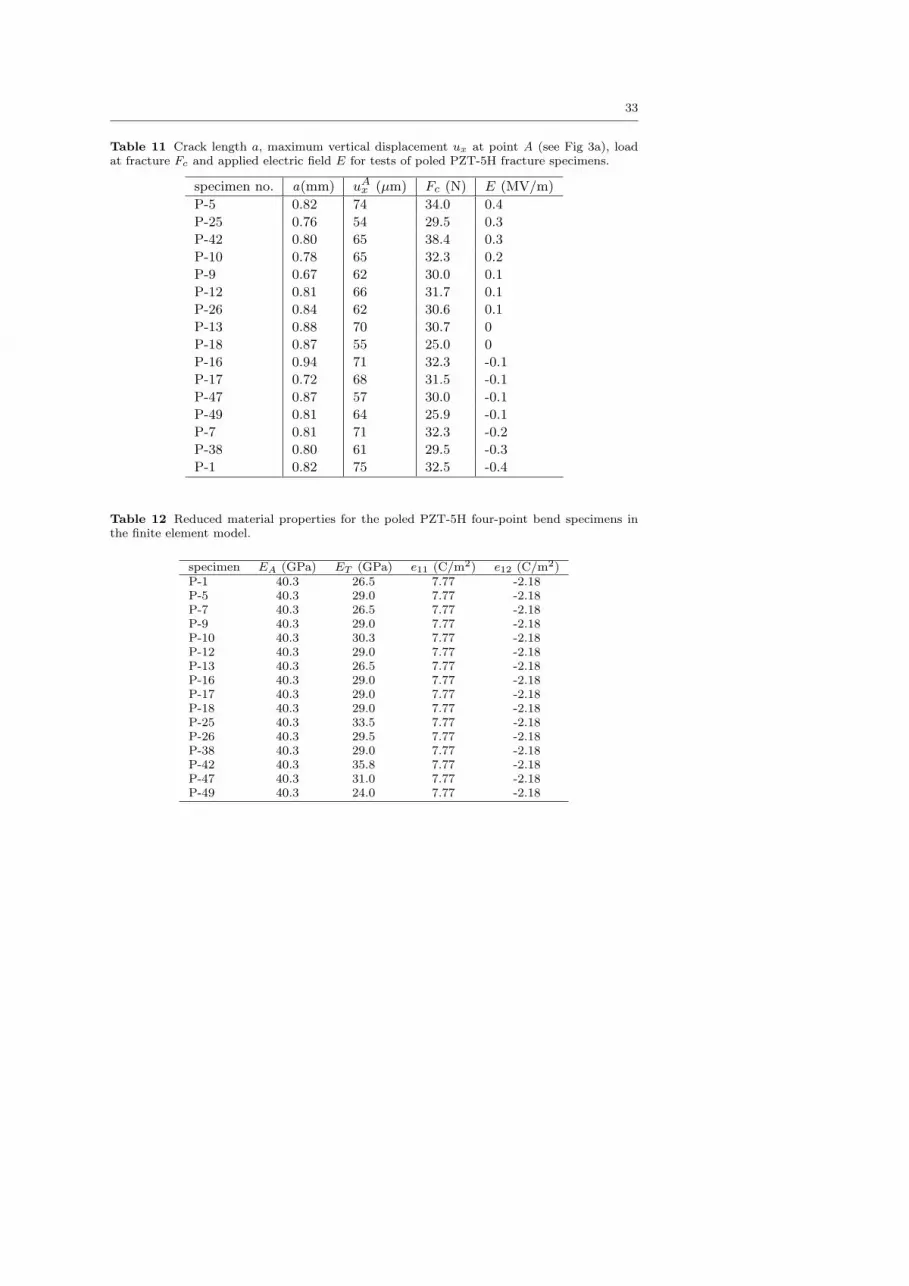
33

Table 11 Crack length a, maximum vertical displacement ux at point A (see Fig 3a), loadat fracture Fc and applied electric field E for tests of poled PZT-5H fracture specimens.

specimen no. a(mm) uAx (µm) Fc (N) E (MV/m)

P-5 0.82 74 34.0 0.4

P-25 0.76 54 29.5 0.3

P-42 0.80 65 38.4 0.3

P-10 0.78 65 32.3 0.2

P-9 0.67 62 30.0 0.1

P-12 0.81 66 31.7 0.1

P-26 0.84 62 30.6 0.1

P-13 0.88 70 30.7 0

P-18 0.87 55 25.0 0

P-16 0.94 71 32.3 -0.1

P-17 0.72 68 31.5 -0.1

P-47 0.87 57 30.0 -0.1

P-49 0.81 64 25.9 -0.1

P-7 0.81 71 32.3 -0.2

P-38 0.80 61 29.5 -0.3

P-1 0.82 75 32.5 -0.4

Table 12 Reduced material properties for the poled PZT-5H four-point bend specimens inthe finite element model.

specimen EA (GPa) ET (GPa) e11 (C/m2) e12 (C/m2)P-1 40.3 26.5 7.77 -2.18P-5 40.3 29.0 7.77 -2.18P-7 40.3 26.5 7.77 -2.18P-9 40.3 29.0 7.77 -2.18P-10 40.3 30.3 7.77 -2.18P-12 40.3 29.0 7.77 -2.18P-13 40.3 26.5 7.77 -2.18P-16 40.3 29.0 7.77 -2.18P-17 40.3 29.0 7.77 -2.18P-18 40.3 29.0 7.77 -2.18P-25 40.3 33.5 7.77 -2.18P-26 40.3 29.5 7.77 -2.18P-38 40.3 29.0 7.77 -2.18P-42 40.3 35.8 7.77 -2.18P-47 40.3 31.0 7.77 -2.18P-49 40.3 24.0 7.77 -2.18