Embed Size (px)
Citation preview

A Comprehensive Piezoelectric Bending-Beam Model Inspired byMicroaerial Vehicle Applications
by
Peter Andras Kovacs Szabo
A thesis submitted in conformity with the requirementsfor the degree of Doctor of Philosophy
Graduate Department of the Institute for Aerospace StudiesUniversity of Toronto
© Copyright 2016 by Peter Andras Kovacs Szabo

Abstract
A Comprehensive Piezoelectric Bending-Beam Model Inspired by Microaerial Vehicle Applications
Peter Andras Kovacs Szabo
Doctor of Philosophy
Graduate Department of the Institute for Aerospace Studies
University of Toronto
2016
Microaerial vehicles are an up-and-coming area of robotics which is fuelled by modern understanding
of the unsteady aerodynamics of insect flight and the development of new actuation technologies. In
the past two decades computer simulations have aided in uncovering the lift mechanisms which flying
insects use to stay aloft. Using these details, roboticists had begun using lightweight structures and high
power density actuators to mimic the physical parameters and flapping kinematics of flying insects with
the intent to recreate the dynamics of insect flight. One of the most important aspects of flapping-wing
microaerial vehicles is the actuation method. Piezoelectric bending-beam actuators have been scaled up
from MEMS technology for use in microaerial vehicle applications owing to their high power density and
performance at low mass.
The initial development toward the UTIAS Robotic Dragonfly, a microaerial vehicle platform using a
piezoelectric-based actuator, is outlined. The components are fabricated from lightweight materials such
as a carbon fibre frame, polymide film joints, and polyester film wings while the actuator is a piezoelectric
bending-beam which was designed using existing mathematical models. The design and fabrication of
the wings, actuator, transmission, and power supply are detailed. The prototypes are measured for
lift generation using custom lift sensors which had undergone static and dynamic calibration for low-
force, high-bandwidth measurement. Although the resulting lift curves qualitatively correspond with
the literature, it was determined that more power was needed for lift-off to be achieved and existing
piezoelectric models do not fully account for maximizing the force-deflection relationship.
An extension to the existing Ballas model of piezoelectric bending-beam devices is derived. This
modified Ballas model incorporates devices beyond constant width. Actuator performance limitations
highlighted the need for a more comprehensive piezoelectric bending-beam model. The final contribution
is a derivation of a new bending-beam model to permit multiple layers, any continuous width profile,
and independent layer excitation. An energy-based approach using the extended Hamilton’s principle
was used to incorporate the generalities desired in the new piezoelectric bending-beam model. Examples
of the new model are compared to both simulation and experiment for verification as well as to showcase
its versatility.
ii

Acknowledgements
This thesis would not have been possible were it not for my parents, Lajos & Margit Szabo. I am
forever grateful to them for instilling in me at an early age the concepts of perseverance and hard work.
They sacrificed everything so that I could have the opportunity to do anything.
I would like to thank my fiancee, Adrienne, for her never-ending support, understanding, and patience
throughout this endeavour. I am lucky to have you in my life and I look forward to wherever the future
takes us. I’m sorry it took so long. I am also indebted to my brother and his wife, David & Florence
Szabo. Both of you have always been so kind and welcoming to me, your support has helped me through
the toughest of times. My fellow undergraduate classmates and closest friends, Sujeev Ruban and Kristen
Yee Loong, thank you for giving me support when I needed support and space when I needed space.
But most importantly, thank you for reminding me to keep things in perspective.
I would like to express my gratitude to my supervisor, Prof. D’Eleuterio, for helping me grow as an
academic, an engineer, and as a person. Gabe, I think I speak for the entire group when I say that you
have nurtured in us an appreciation for more than just academics and scholarship, but also art, history,
literature, politics, sports, and so much more. I can confidently say that I am a much better person now
than when I first arrived. I would also like to thank the other members of my Doctoral Examination
Committee, Prof. DeLaurier and Prof. Liu, for their advice, insight, and guidance. I am grateful to
Prof. Zingg and Prof. Davis for entrusting me with the responsibility of instructing AER525 on my own,
it was an invaluable experience. Along the same vein, I also thank Prof. Emami for providing me with
the opportunity to learn and grow through my teaching assistantships over the years. The expertise of
the faculty of the University of Toronto has been a tremendous resource and I thank Prof. Damaren,
Prof. Steeves, Prof. Sun, and Prof. Weis in particular for being so accommodating and eager to share
their knowledge.
“The real University has no specific location. It owns no property, pays no salaries, and
receives no material dues. The real University is a state of mind. It is that great heritage
of rational thought that has been brought down to us through the centuries and which does
not exist at any specific location. It’s a state of mind which is regenerated throughout the
centuries by a body of people who traditionally carry the title of professor, but even that title
is not part of the real University. The real University is nothing less than the continuing body
of reason itself.”
- Zen and the Art of Motorcycle Maintenance by Robert M. Pirsig (b. 1928)
Other members of the Robotic Dragonfly team deserve recognition for the hard work toward our
common goal, namely: Vidya Menon, Zain Ahmed, Allen Chee, Jai Bansal, Murtaza Bohra, Susan
Choi, Alison McPhail, and Behrad Vatankhahghadim. I would like to thank those who have provided
input and fruitful discussion to help better my thesis, in alphabetical order: Heather Armstrong, David
Beach, Dr. Ernest Earon, Francis Frenzel, Terence Fu, Jonathan Gammell, Dr. Paul Grouchy, Kenneth
Law, Anton Rubisov, Alexander Smith, Adam Sniderman, Dr. Adam Trischler, Dr. Susie Wadgymar,
and Li Zhou.
Even though there is little hope that they would remember me, I would like to express my appreciation
to Prof. Michael Dickinson, Prof. Ronald Fearing, and Prof. Z. Jane Wang for coming to speak at the
University of Toronto and permitting me to bombard them with questions in private afterwards.
iii

Contents
1 Introduction 1
1.1 Motivation . . . . . . . . . . . . . . . . . . . . . . . . . . . . . . . . . . . . . . . . . . . . 2
1.1.1 Why Mimic Nature? . . . . . . . . . . . . . . . . . . . . . . . . . . . . . . . . . . . 2
1.1.2 Biomimetic Microrobotics . . . . . . . . . . . . . . . . . . . . . . . . . . . . . . . . 4
1.1.3 Actuation Technology . . . . . . . . . . . . . . . . . . . . . . . . . . . . . . . . . . 5
1.1.4 Piezoelectric Bending-Beam Models . . . . . . . . . . . . . . . . . . . . . . . . . . 5
1.2 Flapping-Winged Flight at UTIAS . . . . . . . . . . . . . . . . . . . . . . . . . . . . . . . 6
1.3 UTIAS Robotic Dragonfly Project . . . . . . . . . . . . . . . . . . . . . . . . . . . . . . . 7
1.3.1 Thesis Scope . . . . . . . . . . . . . . . . . . . . . . . . . . . . . . . . . . . . . . . 7
1.3.2 Contributions . . . . . . . . . . . . . . . . . . . . . . . . . . . . . . . . . . . . . . . 8
2 Literature Review 10
2.1 The Dragonfly . . . . . . . . . . . . . . . . . . . . . . . . . . . . . . . . . . . . . . . . . . 11
2.1.1 The Fossil Record . . . . . . . . . . . . . . . . . . . . . . . . . . . . . . . . . . . . 11
2.1.2 Morphology . . . . . . . . . . . . . . . . . . . . . . . . . . . . . . . . . . . . . . . . 13
2.1.3 Flight Kinematics . . . . . . . . . . . . . . . . . . . . . . . . . . . . . . . . . . . . 15
2.1.4 Muscle Power . . . . . . . . . . . . . . . . . . . . . . . . . . . . . . . . . . . . . . . 17
2.1.5 Sympetrum sanguineum . . . . . . . . . . . . . . . . . . . . . . . . . . . . . . . . . 19
2.2 Understanding Insect Flight . . . . . . . . . . . . . . . . . . . . . . . . . . . . . . . . . . . 20
2.2.1 Flapping Simulations . . . . . . . . . . . . . . . . . . . . . . . . . . . . . . . . . . . 21
2.2.2 Scaled Flapping Experiments . . . . . . . . . . . . . . . . . . . . . . . . . . . . . . 23
2.2.3 Flight Mechanisms . . . . . . . . . . . . . . . . . . . . . . . . . . . . . . . . . . . . 25
2.3 Microaerial Vehicles . . . . . . . . . . . . . . . . . . . . . . . . . . . . . . . . . . . . . . . 27
2.3.1 Motivation . . . . . . . . . . . . . . . . . . . . . . . . . . . . . . . . . . . . . . . . 28
2.3.2 Applications . . . . . . . . . . . . . . . . . . . . . . . . . . . . . . . . . . . . . . . 28
2.3.3 Existing MAV Projects . . . . . . . . . . . . . . . . . . . . . . . . . . . . . . . . . 28
2.4 Piezoelectric Actuation . . . . . . . . . . . . . . . . . . . . . . . . . . . . . . . . . . . . . . 42
2.4.1 The Piezoelectric Effect . . . . . . . . . . . . . . . . . . . . . . . . . . . . . . . . . 42
2.4.2 History of Piezoelectricity . . . . . . . . . . . . . . . . . . . . . . . . . . . . . . . . 44
2.4.3 Linear Theory of Piezoelectricity . . . . . . . . . . . . . . . . . . . . . . . . . . . . 46
2.4.4 Piezoelectric Bending-Beams . . . . . . . . . . . . . . . . . . . . . . . . . . . . . . 52
2.4.5 Off-the-Shelf Solutions . . . . . . . . . . . . . . . . . . . . . . . . . . . . . . . . . . 54
2.4.6 Existing Piezoelectric Bending-Beam Models . . . . . . . . . . . . . . . . . . . . . 54
iv

3 UTIAS Robotic Dragonfly 67
3.1 The Goal . . . . . . . . . . . . . . . . . . . . . . . . . . . . . . . . . . . . . . . . . . . . . 67
3.1.1 Idealised Dragonfly . . . . . . . . . . . . . . . . . . . . . . . . . . . . . . . . . . . . 68
3.1.2 Future Concept . . . . . . . . . . . . . . . . . . . . . . . . . . . . . . . . . . . . . . 68
3.2 Prototype Design Methodology . . . . . . . . . . . . . . . . . . . . . . . . . . . . . . . . . 69
3.2.1 Overview . . . . . . . . . . . . . . . . . . . . . . . . . . . . . . . . . . . . . . . . . 69
3.2.2 Wings . . . . . . . . . . . . . . . . . . . . . . . . . . . . . . . . . . . . . . . . . . . 71
3.2.3 Actuator . . . . . . . . . . . . . . . . . . . . . . . . . . . . . . . . . . . . . . . . . 74
3.2.4 Transmission . . . . . . . . . . . . . . . . . . . . . . . . . . . . . . . . . . . . . . . 79
3.2.5 Frame . . . . . . . . . . . . . . . . . . . . . . . . . . . . . . . . . . . . . . . . . . . 82
3.2.6 Power Supply . . . . . . . . . . . . . . . . . . . . . . . . . . . . . . . . . . . . . . . 83
3.3 Actuator-Transmission-Wing (ATW) System . . . . . . . . . . . . . . . . . . . . . . . . . 85
3.3.1 Energy-Based Model . . . . . . . . . . . . . . . . . . . . . . . . . . . . . . . . . . . 86
3.3.2 Model of the ATW System . . . . . . . . . . . . . . . . . . . . . . . . . . . . . . . 88
3.3.3 Overall System of Equations . . . . . . . . . . . . . . . . . . . . . . . . . . . . . . 92
3.3.4 Usability of the ATW Model . . . . . . . . . . . . . . . . . . . . . . . . . . . . . . 93
3.3.5 Resonant Behaviour . . . . . . . . . . . . . . . . . . . . . . . . . . . . . . . . . . . 94
3.4 Lift Measurement Set-Up . . . . . . . . . . . . . . . . . . . . . . . . . . . . . . . . . . . . 95
3.4.1 Existing Solutions . . . . . . . . . . . . . . . . . . . . . . . . . . . . . . . . . . . . 95
3.4.2 Requirements . . . . . . . . . . . . . . . . . . . . . . . . . . . . . . . . . . . . . . . 96
3.4.3 Design . . . . . . . . . . . . . . . . . . . . . . . . . . . . . . . . . . . . . . . . . . . 96
3.4.4 Calibration . . . . . . . . . . . . . . . . . . . . . . . . . . . . . . . . . . . . . . . . 99
3.5 Summary of 2P Platform Iterations . . . . . . . . . . . . . . . . . . . . . . . . . . . . . . . 106
3.6 Experimentation . . . . . . . . . . . . . . . . . . . . . . . . . . . . . . . . . . . . . . . . . 108
3.6.1 Resonance Testing . . . . . . . . . . . . . . . . . . . . . . . . . . . . . . . . . . . . 108
3.6.2 Prototype Testing . . . . . . . . . . . . . . . . . . . . . . . . . . . . . . . . . . . . 108
3.6.3 Comparison to Literature . . . . . . . . . . . . . . . . . . . . . . . . . . . . . . . . 116
4 Modified Ballas Model 121
4.1 Review of Ballas Model Rectangular Formulation . . . . . . . . . . . . . . . . . . . . . . . 121
4.2 Modified Ballas Model Problem Set-Up . . . . . . . . . . . . . . . . . . . . . . . . . . . . 125
4.2.1 General Width Function . . . . . . . . . . . . . . . . . . . . . . . . . . . . . . . . . 125
4.2.2 Flexural Rigidity for the General Width Case . . . . . . . . . . . . . . . . . . . . . 126
4.2.3 Piezoelectric Bending Moment for the General Width Case . . . . . . . . . . . . . 126
4.3 Modified Ballas Model General Width Formulation . . . . . . . . . . . . . . . . . . . . . . 127
4.3.1 Applied Torque . . . . . . . . . . . . . . . . . . . . . . . . . . . . . . . . . . . . . . 127
4.3.2 Applied Force . . . . . . . . . . . . . . . . . . . . . . . . . . . . . . . . . . . . . . . 129
4.3.3 Applied Uniform Pressure Load . . . . . . . . . . . . . . . . . . . . . . . . . . . . . 130
4.3.4 Electric Charge . . . . . . . . . . . . . . . . . . . . . . . . . . . . . . . . . . . . . . 131
4.4 Common Configurations . . . . . . . . . . . . . . . . . . . . . . . . . . . . . . . . . . . . . 136
4.4.1 Rectangular Case . . . . . . . . . . . . . . . . . . . . . . . . . . . . . . . . . . . . . 137
4.4.2 Trapezoidal Case . . . . . . . . . . . . . . . . . . . . . . . . . . . . . . . . . . . . . 137
4.4.3 Parabolic Case . . . . . . . . . . . . . . . . . . . . . . . . . . . . . . . . . . . . . . 138
4.4.4 Higher-Order Cases . . . . . . . . . . . . . . . . . . . . . . . . . . . . . . . . . . . 138
v

5 New Actuator Model 139
5.1 Problem Set-Up . . . . . . . . . . . . . . . . . . . . . . . . . . . . . . . . . . . . . . . . . . 139
5.2 General Multilayered Piezoelectric Beam . . . . . . . . . . . . . . . . . . . . . . . . . . . . 142
5.2.1 Extended Hamilton’s Principle . . . . . . . . . . . . . . . . . . . . . . . . . . . . . 142
5.2.2 Equations of Equilibrium . . . . . . . . . . . . . . . . . . . . . . . . . . . . . . . . 144
5.3 Finite-Element Model . . . . . . . . . . . . . . . . . . . . . . . . . . . . . . . . . . . . . . 145
5.3.1 Discretized Equations of Equilibrium . . . . . . . . . . . . . . . . . . . . . . . . . . 146
5.3.2 Engineering Constitutive Relations . . . . . . . . . . . . . . . . . . . . . . . . . . . 146
5.3.3 Change of Variables . . . . . . . . . . . . . . . . . . . . . . . . . . . . . . . . . . . 147
5.3.4 Layer-Based vs. Source-Based Representation . . . . . . . . . . . . . . . . . . . . . 147
5.4 Application of the Model . . . . . . . . . . . . . . . . . . . . . . . . . . . . . . . . . . . . 148
5.4.1 Boundary Conditions . . . . . . . . . . . . . . . . . . . . . . . . . . . . . . . . . . 148
5.4.2 Global Behaviour of Cantilever Case . . . . . . . . . . . . . . . . . . . . . . . . . . 149
5.4.3 Local Behaviour of a Beam . . . . . . . . . . . . . . . . . . . . . . . . . . . . . . . 149
5.4.4 Common Cases . . . . . . . . . . . . . . . . . . . . . . . . . . . . . . . . . . . . . . 149
5.4.5 Multisource Cases . . . . . . . . . . . . . . . . . . . . . . . . . . . . . . . . . . . . 151
5.5 Simulation . . . . . . . . . . . . . . . . . . . . . . . . . . . . . . . . . . . . . . . . . . . . . 151
5.6 Experimental Procedure . . . . . . . . . . . . . . . . . . . . . . . . . . . . . . . . . . . . . 153
5.6.1 Piezoceramic: PZT-5H . . . . . . . . . . . . . . . . . . . . . . . . . . . . . . . . . . 153
5.6.2 Experimental Set-up . . . . . . . . . . . . . . . . . . . . . . . . . . . . . . . . . . . 154
5.7 Experiments . . . . . . . . . . . . . . . . . . . . . . . . . . . . . . . . . . . . . . . . . . . . 156
5.7.1 Experiment 1: Verification of New Model . . . . . . . . . . . . . . . . . . . . . . . 156
5.7.2 Experiment 2: Quadratic Width Profile . . . . . . . . . . . . . . . . . . . . . . . . 160
5.7.3 Experiment 3: Independent Layer Drive . . . . . . . . . . . . . . . . . . . . . . . . 163
5.7.4 Experiment 4: Nontraditional Boundary Conditions . . . . . . . . . . . . . . . . . 165
5.7.5 Discussion . . . . . . . . . . . . . . . . . . . . . . . . . . . . . . . . . . . . . . . . . 168
6 Conclusion 170
6.1 Future Work . . . . . . . . . . . . . . . . . . . . . . . . . . . . . . . . . . . . . . . . . . . 171
6.1.1 Lift Measurement System Upgrade . . . . . . . . . . . . . . . . . . . . . . . . . . . 171
6.1.2 On-Board Power Supply . . . . . . . . . . . . . . . . . . . . . . . . . . . . . . . . . 172
6.1.3 Dynamic Actuator Model . . . . . . . . . . . . . . . . . . . . . . . . . . . . . . . . 173
6.1.4 Optimization of UTIAS Robotic Dragonfly Actuator . . . . . . . . . . . . . . . . . 173
6.1.5 Alternative Actuator Materials . . . . . . . . . . . . . . . . . . . . . . . . . . . . . 173
6.2 Contributions . . . . . . . . . . . . . . . . . . . . . . . . . . . . . . . . . . . . . . . . . . . 173
6.3 Closing Thoughts . . . . . . . . . . . . . . . . . . . . . . . . . . . . . . . . . . . . . . . . . 174
Appendix A: UTIAS Robotic Dragonfly Design Schematics 175
Appendix B: Power Supply Circuit Diagram 183
Appendix C: Lift Sensor Circuit Diagrams 185
Bibliography 187
vi

List of Tables
2.1 Sympetrum sanguineum physical parameters from Wakeling & Ellington [141,143] . . . . 20
2.2 Sympetrum sanguineum performance parameters from Wakeling & Ellington [142,143] . . 20
2.3 Comparison of DelFly platforms . . . . . . . . . . . . . . . . . . . . . . . . . . . . . . . . 29
2.4 Comparison of Cornell University Hovering MAV platforms . . . . . . . . . . . . . . . . . 31
2.5 Comparison of Carnegie Mellon University hovering MAV platforms . . . . . . . . . . . . 32
2.6 Comparison of University of Delaware/Purdue University MAV platforms . . . . . . . . . 34
2.7 Micromechanical Flying Insect properties . . . . . . . . . . . . . . . . . . . . . . . . . . . 35
2.8 Comparison of Harvard University MAV platforms . . . . . . . . . . . . . . . . . . . . . . 38
2.9 List of classic thermodynamic potentials [5] . . . . . . . . . . . . . . . . . . . . . . . . . . 46
2.10 List of intensive and extensive variables . . . . . . . . . . . . . . . . . . . . . . . . . . . . 48
2.11 List of thermodynamic functions [84] . . . . . . . . . . . . . . . . . . . . . . . . . . . . . . 48
2.12 List of constitutive equation pairs [71,84] . . . . . . . . . . . . . . . . . . . . . . . . . . . 48
2.13 Compressed matrix notation . . . . . . . . . . . . . . . . . . . . . . . . . . . . . . . . . . . 51
2.14 Highlights and limitations of the Smits et al. model . . . . . . . . . . . . . . . . . . . . . 56
2.15 Highlights and limitations of the Ballas model . . . . . . . . . . . . . . . . . . . . . . . . . 57
2.16 Highlights and limitations of the Tabesh & Frechette model . . . . . . . . . . . . . . . . . 59
2.17 Highlights and limitations of the Fernandes & Pouget model . . . . . . . . . . . . . . . . . 60
2.18 Highlights and limitations of the Wood et al. model . . . . . . . . . . . . . . . . . . . . . 61
2.19 Highlights and limitations of the Tiersten model . . . . . . . . . . . . . . . . . . . . . . . 62
2.20 Highlights and limitations of the Tanaka model . . . . . . . . . . . . . . . . . . . . . . . . 63
2.21 Highlights and limitations of the Erturk & Inman model . . . . . . . . . . . . . . . . . . . 65
3.1 Idealised Dragonfly overall body parameters . . . . . . . . . . . . . . . . . . . . . . . . . . 68
3.2 Idealised Dragonfly wing physical parameters . . . . . . . . . . . . . . . . . . . . . . . . . 68
3.3 Idealised Dragonfly wing kinematic specifications . . . . . . . . . . . . . . . . . . . . . . . 68
3.4 Spanwise and chordwise stiffness of dragonfly wings based on Combes & Daniel [21] . . . 72
3.5 Properties of the artificial dragonfly wings . . . . . . . . . . . . . . . . . . . . . . . . . . . 74
3.6 Summary of actuator models used . . . . . . . . . . . . . . . . . . . . . . . . . . . . . . . 76
3.7 PZT-5H piezoceramic properties from Piezo Systems, Inc. [98] . . . . . . . . . . . . . . . . 76
3.8 A sample of some of the actuators designed and fabricated . . . . . . . . . . . . . . . . . . 77
3.9 Comparison of drive configuration performance . . . . . . . . . . . . . . . . . . . . . . . . 77
3.10 Comparison of planform configuration performance . . . . . . . . . . . . . . . . . . . . . . 79
3.11 Comparison of rectangular vs wide-base trapezoidal planform performance . . . . . . . . . 79
3.12 Tracking the change in `2 in the second platform . . . . . . . . . . . . . . . . . . . . . . . 81
vii

3.13 Power supply requirements . . . . . . . . . . . . . . . . . . . . . . . . . . . . . . . . . . . 84
3.14 Dual drive circuit phase relationships . . . . . . . . . . . . . . . . . . . . . . . . . . . . . . 85
3.15 Summary of properties of components of interest . . . . . . . . . . . . . . . . . . . . . . . 88
3.16 List of parameters for 2P12 relevant to the ATW system . . . . . . . . . . . . . . . . . . . 94
3.17 List of lift sensor requirements . . . . . . . . . . . . . . . . . . . . . . . . . . . . . . . . . 96
3.18 Comparison of SMD load cells S100 and S2154 . . . . . . . . . . . . . . . . . . . . . . . . 98
3.19 Specifications of the DAQ: (MCC USB-1608G5) . . . . . . . . . . . . . . . . . . . . . . . . 98
3.20 Expected performance for the S100-based and S215-based amplification circuits . . . . . . 99
3.21 List of precision masses . . . . . . . . . . . . . . . . . . . . . . . . . . . . . . . . . . . . . 100
3.22 Motorized calibrator parameters . . . . . . . . . . . . . . . . . . . . . . . . . . . . . . . . 102
3.23 Summary of physical parameters of select platform iterations . . . . . . . . . . . . . . . . 106
3.24 List of natural frequencies for select prototype iterations . . . . . . . . . . . . . . . . . . . 108
3.25 List of quantitative results for 2P20 at the seven wingbeat frequencies of interest . . . . . 111
3.26 Comparison of mean lift between experiment and simulation . . . . . . . . . . . . . . . . . 118
3.27 Comparison of lift coefficients between experiment and simulation . . . . . . . . . . . . . 119
5.1 Sample of width functions (0 ≤ x ≤ `) . . . . . . . . . . . . . . . . . . . . . . . . . . . . . 140
5.2 List of intensive and extensive variables . . . . . . . . . . . . . . . . . . . . . . . . . . . . 140
5.3 Experiment 1: physical parameters . . . . . . . . . . . . . . . . . . . . . . . . . . . . . . . 156
5.4 Experiment 1 Case 1: applied 100 mN tip force, charge fixed . . . . . . . . . . . . . . . . 158
5.5 Experiment 1 Case 2: applied 100 mN tip force, charge nonfixed . . . . . . . . . . . . . . 159
5.6 Experiment 1 Case 3: contemporary models applied 41.5 V potential . . . . . . . . . . . . 160
5.7 Experiment 1 Case 3: applied 41.5 V potential . . . . . . . . . . . . . . . . . . . . . . . . 160
5.8 Experiment 2: physical parameters . . . . . . . . . . . . . . . . . . . . . . . . . . . . . . . 161
5.9 Experiment 2 Case 1: applied 100 mN tip force, charge fixed . . . . . . . . . . . . . . . . 161
5.10 Experiment 2 Case 2: applied 100 mN tip force, charge nonfixed . . . . . . . . . . . . . . 162
5.11 Experiment 2 Case 3: applied 41.5 V potential . . . . . . . . . . . . . . . . . . . . . . . . 163
5.12 Experiment 3: physical parameters . . . . . . . . . . . . . . . . . . . . . . . . . . . . . . . 164
5.13 Experiment 3: applied ΦA = 41.5 V and ΦB = 32.5 V . . . . . . . . . . . . . . . . . . . . 165
5.14 Experiment 4: physical parameters . . . . . . . . . . . . . . . . . . . . . . . . . . . . . . . 166
5.15 Experiment 4: applied 41.5 V potential . . . . . . . . . . . . . . . . . . . . . . . . . . . . 168
viii

List of Figures
1.1 Early attempts at manned flight . . . . . . . . . . . . . . . . . . . . . . . . . . . . . . . . 2
1.2 Examples of early small-scale flapping-wing development at UTIAS . . . . . . . . . . . . . 6
2.1 Genus Meganeura dated from the Carboniferous period (300 million years ago) . . . . . . 12
2.2 Highlights of dragonfly morphology . . . . . . . . . . . . . . . . . . . . . . . . . . . . . . . 14
2.3 Comparison of flying insect stroke planes during hovering [150] . . . . . . . . . . . . . . . 16
2.4 Comparison of insect flight muscles2 . . . . . . . . . . . . . . . . . . . . . . . . . . . . . . 18
2.5 Sympetrum sanguineum [7] . . . . . . . . . . . . . . . . . . . . . . . . . . . . . . . . . . . 20
2.6 Various DelFly platforms . . . . . . . . . . . . . . . . . . . . . . . . . . . . . . . . . . . . 30
2.7 Various Cornell University hovering MAV platforms . . . . . . . . . . . . . . . . . . . . . 31
2.8 Various Carnegie Mellon University MAV platforms . . . . . . . . . . . . . . . . . . . . . 33
2.9 Various University of Delaware/Purdue University MAV platforms . . . . . . . . . . . . . 34
2.10 Highlights of the Micromechanical Flying Insect . . . . . . . . . . . . . . . . . . . . . . . . 35
2.11 Various Harvard University MAV platforms . . . . . . . . . . . . . . . . . . . . . . . . . . 38
2.12 Harvard “pop-up” monolithic assembly method [124] . . . . . . . . . . . . . . . . . . . . . 39
2.13 Active control of the wing hinge rest position of the Harvard RoboBee [133] . . . . . . . . 41
2.14 Piezoelectric crystal structure (a) above and (b) below the Curie temperature [10] . . . . 43
2.15 Comparison of piezoelectric crystal regions throughout the poling process . . . . . . . . . 44
2.16 Bending caused by piezoelectric effect (piezoelectric upper, elastic lower) . . . . . . . . . . 53
2.17 Examples of typical drive methods for bimorph actuators . . . . . . . . . . . . . . . . . . 53
2.18 Highlights of the Ballas multilayered piezoelectric bending-beam model [10] . . . . . . . . 58
2.19 Tanaka configuration [132] . . . . . . . . . . . . . . . . . . . . . . . . . . . . . . . . . . . . 64
3.1 Artistic rendition of future UTIAS Robotic Dragonfly . . . . . . . . . . . . . . . . . . . . 69
3.2 Major components of the UTIAS Robotic Dragonfly prototype . . . . . . . . . . . . . . . 70
3.3 Comparison of the two UTIAS Robotic Dragonfly piezoelectric-based platforms . . . . . . 71
3.4 Dragonfly hindwing venation pattern comparison [79] . . . . . . . . . . . . . . . . . . . . . 72
3.5 Artificial wings of the UTIAS Robotic Dragonfly . . . . . . . . . . . . . . . . . . . . . . . 74
3.6 Examples of drive configurations and width planforms used . . . . . . . . . . . . . . . . . 75
3.7 Comparison of force-displacement curves for select cases . . . . . . . . . . . . . . . . . . . 78
3.8 Overview of the transmission mechanism . . . . . . . . . . . . . . . . . . . . . . . . . . . . 80
3.9 Transmission kinematics throughout the stroke period . . . . . . . . . . . . . . . . . . . . 80
3.10 Select prototypes with assembled ATW systems . . . . . . . . . . . . . . . . . . . . . . . . 82
3.11 Overview of the dual drive circuit . . . . . . . . . . . . . . . . . . . . . . . . . . . . . . . . 85
ix

3.12 Positioning of the body frame B and stroke-plane frame S . . . . . . . . . . . . . . . 87
3.13 Summary of relevant properties of the ATW system . . . . . . . . . . . . . . . . . . . . . 88
3.14 Detailed diagrams of each ATW body with parameters defined . . . . . . . . . . . . . . . 89
3.15 Load cell options and completed lift sensors . . . . . . . . . . . . . . . . . . . . . . . . . . 97
3.16 Overview of the lift sensor circuit . . . . . . . . . . . . . . . . . . . . . . . . . . . . . . . . 99
3.17 Static calibration transformation results . . . . . . . . . . . . . . . . . . . . . . . . . . . . 101
3.18 Dynamic calibration device details . . . . . . . . . . . . . . . . . . . . . . . . . . . . . . . 103
3.19 S100-based lift sensor dynamic results . . . . . . . . . . . . . . . . . . . . . . . . . . . . . 104
3.20 S215-based lift sensor dynamic results . . . . . . . . . . . . . . . . . . . . . . . . . . . . . 105
3.21 CAD models of the 2P# platform iterations of interest . . . . . . . . . . . . . . . . . . . . 107
3.22 Downstroke and upstroke for 2P16T at 14.2 Hz wingbeat frequency . . . . . . . . . . . . 110
3.23 Downstroke and upstroke for 2P20 at 25.0 Hz wingbeat frequency . . . . . . . . . . . . . 111
3.24 Experimental results for 2P20 at 15.1 Hz wingbeat frequency . . . . . . . . . . . . . . . . 112
3.25 Experimental results for 2P20 at 20.0 Hz wingbeat frequency . . . . . . . . . . . . . . . . 113
3.26 Experimental results for 2P20 at 25.0 Hz wingbeat frequency . . . . . . . . . . . . . . . . 113
3.27 Experimental results for 2P20 at 27.6 Hz wingbeat frequency . . . . . . . . . . . . . . . . 114
3.28 Experimental results for 2P20 at 30.1 Hz wingbeat frequency . . . . . . . . . . . . . . . . 114
3.29 Experimental results for 2P20 at 32.5 Hz wingbeat frequency . . . . . . . . . . . . . . . . 115
3.30 Experimental results for 2P20 at 38.3 Hz wingbeat frequency . . . . . . . . . . . . . . . . 115
3.31 Comparison of 2P20 experimental results to simulation . . . . . . . . . . . . . . . . . . . 119
4.1 Highlights of Ballas multilayered piezoelectric bending-beam model . . . . . . . . . . . . . 122
4.2 Planform view of an actuator with width as a function of x . . . . . . . . . . . . . . . . . 126
5.1 Overview of a generalized piezoelectric bending-beam . . . . . . . . . . . . . . . . . . . . 140
5.2 Breakdown of a generalized multilayered beam . . . . . . . . . . . . . . . . . . . . . . . . 141
5.3 A generalized multimorph . . . . . . . . . . . . . . . . . . . . . . . . . . . . . . . . . . . . 141
5.4 Examples of physical boundary conditions . . . . . . . . . . . . . . . . . . . . . . . . . . . 148
5.5 Configuration examples . . . . . . . . . . . . . . . . . . . . . . . . . . . . . . . . . . . . . 150
5.6 Individual elements in the x and z directions . . . . . . . . . . . . . . . . . . . . . . . . . 152
5.7 Example of a fabricated bending-beam test sample . . . . . . . . . . . . . . . . . . . . . . 153
5.8 Experimental set-up used during testing . . . . . . . . . . . . . . . . . . . . . . . . . . . . 155
5.9 Experiment 1: physical set-up . . . . . . . . . . . . . . . . . . . . . . . . . . . . . . . . . . 156
5.10 Experiment 1 Case 1: applied 100 mN tip force, charge fixed . . . . . . . . . . . . . . . . 159
5.11 Experiment 1 Case 2: applied 100 mN tip force, charge nonfixed . . . . . . . . . . . . . . 159
5.12 Experiment 1 Case 3: applied 41.5 V potential . . . . . . . . . . . . . . . . . . . . . . . . 160
5.13 Experiment 2: physical set-up . . . . . . . . . . . . . . . . . . . . . . . . . . . . . . . . . . 161
5.14 Experiment 2 Case 1: applied 100 mN tip force, charge fixed . . . . . . . . . . . . . . . . 162
5.15 Experiment 2 Case 2: applied 100 mN tip force, charge nonfixed . . . . . . . . . . . . . . 162
5.16 Experiment 2 Case 3: applied 41.5 V potential . . . . . . . . . . . . . . . . . . . . . . . . 163
5.17 Experiment 3: physical set-up . . . . . . . . . . . . . . . . . . . . . . . . . . . . . . . . . . 164
5.18 Experiment 3: applied ΦA = 41.5 V and ΦB = 32.5 V . . . . . . . . . . . . . . . . . . . . 166
5.19 Experiment 4: physical set-up . . . . . . . . . . . . . . . . . . . . . . . . . . . . . . . . . . 167
5.20 Experiment 4: applied 41.5 V potential . . . . . . . . . . . . . . . . . . . . . . . . . . . . 168
x

“Any sufficiently advanced technology
is indistinguishable from magic.”
- Sir Arthur C. Clarke (1917-2008)
Chapter 1
Introduction
Mankind has long had a fascination with flight. Most early attempts at manned flight followed a
biomimetic approach with the hope that flapping a large pair of wings the way birds do would make
them soar into the sky. A famous example is Leonardo da Vinci’s flying machine from the late 1400s;
the wings, through rope and pulleys, were designed to be actuated by a pilot while a tail was intended
to function much like that of a bird. This is also the fashion that Otto Lillenthal attempted, his kleiner
Schlagflugelapparat in the 1890s had wings strapped to the arms of a person as they feverishly attempted
to take-off - always failing. Try as they might, neither da Vinci’s nor Lillenthal’s designs ever flew and it
took until the early 20th century before Orville & Wilbur Wright became the first to achieve sustained,
powered, manned flight. On December 17, 1903 at Kill Devil Hills, North Carolina, Wilbur Wright
piloted the Wright Flyer for 59 s covering a distance of 852 ft on the fourth and final flight of the
day. Their success can be attributed to the attention to four primary factors: aerodynamics, structure,
power, and control. They lived in a time where the understanding of aerodynamics led to a flurry of
research on airfoils, engines, and lightweight frames. They themselves, having spent years building and
repairing printing presses and bicycles, had constructed their own wind-tunnels in order to experiment
with airfoils in their workshop. Also necessary was the development of a strong and light frame which
could hold the wings together and carry a pilot plus engine. Only prior to that had combustion engines
become efficient enough for powered flight to be remotely plausible. Finally, the Wright brothers had
the ingenuity to develop a method of roll control which revolutionised the approach to flight. Many
contemporary designers had pitch and yaw control figured out by using some derivative of an elevator
and a rudder, but it was wing-warping devised by the Wright brothers which permitted the ability to
adjust roll and allowed them to stay in the air for more than a few moments. What is important here
is that manned flight came about because of a timely collision of technological advancement and an
understanding of the physics at play. Without any one of the four areas of development (aerodynamics,
structure, power, and control), the Wright brothers arguably would not have succeeded.
We are once again nearing a revolutionary time regarding a milestone in man-made flight: recreating
insect flight. Even when the Wright brothers were about to make their historic flights, their contem-
poraries, and society in general knew that it would only be a matter of time before someone would
achieve manned flight. The flight of insects, however, seemed like such an impossibility to mimic at
the time. Insect wings flapped at such a fast rate that the human eye could not decipher what was
going on. Motion picture cameras were still in their infancy and it would be decades before frame rates
1

2 Chapter 1. Introduction
(a) Otto Lilienthal (1894) (b) Wright Flyer (1903)
Figure 1.1: Early attempts at manned flight
would become fast enough to catch a glimpse of insect wings in action. Fast-forward to today, it is
now coming to a time where another collision of technological advancement and an understanding of the
physics will make the recreation of insect flight a reality. The development of actuation methods, such
as piezoelectric bending-beams, which are extremely light-weight yet high in power density can actually
meet or exceed that of real insects [159]. The task of dealing with very high wingbeat frequencies also
tests the limits of nature, and by observing the use of resonance in insect exoskeletons during flight can
provide guidance to engineers [59]. Just as important is the aerodynamic understanding of what goes
on around a flapping wing. It is simply not valid to assume a quasisteady analysis of the aerodynamics
of an insect wing flapping at a constant wingbeat frequency [42]. It has only been within the last couple
of decades that it can confidently be said how insects generate lift [138]. There are lift mechanisms
which do not play significant roles in the conventional laminar flow regime of fixed-wing aircraft but
are vital to insect flight, such as clap-and-fling or delayed stall. The primary driving force behind this
new understanding of aerodynamics has been the rapid advancement in computation technology and the
widespread accessibility and power of modern computer simulations. Suddenly, dealing with equations
which had previously been seen as too computationally immense to do by hand can now be done by a
computer in mere minutes if not moments.
1.1 Motivation
The main areas of interest in the pursuit of insect flight recreation is in aerodynamics and actuation.
In developing small-scale robotic insects, much can be learned about the unsteady aerodynamic lift
mechanisms which allow them to fly. Also, the gains in actuator technology are essential for future
microrobotic development as well as any field which makes use of lightweight actuators and sensors.
1.1.1 Why Mimic Nature?
Insects have developed a unique method to fight over the past hundreds of millions of years of evolution.
Large flying creatures, such as birds or bats, flap their wings at a much slower rate than insects. This
is because insects have a much greater reliance on unsteady lift mechanisms which is attributed to
their small size. Insects can afford much higher wing-beat frequencies since all of their flight muscle is
in their thorax while their wings are almost completely passive, rigid structures protruding from the
body [23]. Much of what man has taken advantage of in order to get humans off the ground is very
different than how an insect gets airborne. If a conventional fixed-wing aircraft were to be reduced to
the size of an insect, in order to maintain a similar flow regime, the aircraft would likely have to increase

1.1. Motivation 3
its translational speed well beyond what is technologically feasible or practical at this point [22]. The
solution to artificial flight at very small scales appears to be the use of the same unsteady lift mechanisms
to that of insects.
There are many different types of flying insect with a wide range of wing configurations, sizes, stroke
patterns, and wing-beat frequencies. Where does one begin? Based on the fossil record, some insect
varieties have been around long enough to watch many others come and go. That is to say, some utilize
ancient flying techniques which are much more primitive than other more modern insects. Some of the
first fliers appear to have existed over 350 million years ago and bear a striking resemblance to modern
day dragonflies [42]. Like these modern counterparts, the flight muscles were simple and powered four
wings arranged in two pairs. In fact, modern dragonflies appear virtually unchanged in configuration
right down to similar venation patterns of the wings [23]. More recently evolved insects, such as flies or
bees, have only a single pair of wings and more complex flight musculature which allows for even higher
wing-beat frequencies [16]. Some of these more modern insects utilise complex wing kinematics, such
as clap-and-fling or stroke-plane deviation, which are not normally observed in dragonfly flight. Yet,
dragonflies are still considered some of the most manoeuvrable flying insects to date; that they have
survived for hundreds of millions of years with minimal change is a testament to that.
One interesting phenomenon that many flying insects take advantage of is resonance. The thorax,
where the insect flight muscle is located, behaves as a resonant structure in tune with the operating
wing-beat frequency of the insect. It is believed that in this way insects are able to maximize efficiency
for flight [16]. At resonance, large amplitudes can result from small effort. In both nature and in robotics,
resonance is an integral part of small-scale flapping flight.
Some unique understanding can only come about through experimentation and observation. A simu-
lation is only as good as the assumptions and model simplifications made whereas a physical experiment
can expose some unanticipated results if sufficient detail is included. For example, in 2011 at the Uni-
versity of California, Berkeley, a team led by Ronald Fearing was experimenting with a bipedal running
microrobot which had proven to be unstable during rapid running as it would lose balance and fall over
at high speeds [14]. When experimenting by progressively adding spars, then fixed wings, and eventually
flapping wings to the robot, each addition demonstrated better stability and allowed the robot to run
faster and climb steeper inclines without toppling over. Here, the addition of flapping wings were shown
to be by far more advantageous to the “success” of a running microrobot [97]. What is interesting
about this is that a hypothesis crystallized as to how flight had evolved in nature hundreds of millions of
years ago. The evolutionary origins of flight remain a contentious area amongst evolutionary biologists,
both paleontologically and biomechanically, but it has been suggested that running creatures developed
protrusions out of their thoracic wall for inertial stability [23]. This change could have provided an
evolutionary advantage by improving stability and thus possibly allowing them to escape predators or
reach spaces unattainable than those without. Perhaps this adaptation improved the likelihood of sur-
vival and thus allowed the genes of these early adopters to propagate. The extensions could have grown
membranes over time and eventually became actively moveable by flexing thoracic muscles. This could
very well be how insect flight came about and the aforementioned robotic experiment reinforces this
hypothesis [96]. An insect with moveable, membrane-covered spars, moving fast enough to lift-off or
glide would provide an evolutionary advantage to survive. These kinds of discovery are just some of the
many unknowns which are revealed during robotic experimentation, and it is possible that simulation
alone would not have generated this idea.

4 Chapter 1. Introduction
1.1.2 Biomimetic Microrobotics
The name given to flying robots of the scale of insects is microaerial vehicles (MAVs). The definition
is intentionally vague as an MAV has come to describe not just insect-mimicking flapping-wing robots,
but also fixed-wing aircraft and rotorcraft of very small size. An MAV is generally accepted to be any
flying robot of centimetre-scale while commonly being less than 20 cm in its largest dimension. This
thesis will focus primarily on flapping-wing MAVs.
The list of applications of flapping-wing MAVs are wide and varied. Obvious examples are those which
make use of their small size and biomimetic appearance in order to be discrete, such as surveillance and
reconnaissance for example. A great advantage of flapping-wing MAVs is that their manoeuvrability
combined with small size makes them versatile, cheap, and expendable. Ideal applications such as search
& rescue, exploration of hazardous environments, and traversing cluttered environments take advantage
of this [161,171]. Many police departments and militaries currently use large, often solitary, unmanned
aerial vehicles (UAVs) to perform tasks such as crowd monitoring. Drawbacks of a such large UAV is
that it is often very expensive, upwards of $100, 000 each, limited in effectiveness by having only the
single drone to cover a potentially large area, and debilitating in the event that a technical malfunction
causes the entire mission to come to a halt [160]. Instead, a swarm of MAVs could be used to cover more
area, more quickly, and for less cost. Even if a small number of MAVs are lost, the swarm’s ability to
complete the mission would not be appreciably compromised.
There has been a number of flapping-wing MAV projects to date, some only superficially share
flapping wings in common with insects and nothing more while others strive to be more thoroughly
biomimetic. An example of a loosely insect-mimicking MAV is the DelFly Micro from the Delft University
of Technology which has two pairs of wings clapping together in the same plane but also has a rudder
and elevator at the rear much like a conventional airplane. This MAV does have wings which flap, but
the wing design, flapping kinematics, body mass, and control surfaces do not conform to anything found
in nature.
The first realistic attempt at the development of a true biomimetic MAV came from the University
of California, Berkeley in the late 1990s and was called the Micromechanical Flying Insect (MFI) [14].
What is meant by realistic is that the structural and actuation technology was similar to the mass,
stiffness, and power generated by real insects of comparable size. It was able to control its wings with
two degrees of freedom and could generate lift, albeit not enough to achieve lift-off. Even though it was
not entirely successful, the MFI project laid the foundation for much of the field of insect-inspired MAV
research today. Many of the current primary investigators of the leading MAV research groups across
the United States had at one time formed the original core of researchers for the MFI project over a
decade ago. Some of these members being Robert Wood now at Harvard University, Metin Sitti now at
Carnegie Mellon University, and Xinyan Deng now at Purdue University to name several.
To date, the most successful MAV project is the RoboBee from Harvard University under Robert
Wood [60]. A simplified actuation method where a single piezoelectric actuator and an otherwise bare-
bones prototype tethered to an off-board power supply achieved lift-off in 2007. Since then, the group has
added roll, pitch, and yaw control capabilities and are currently working on on-board sensor integration.
The wing kinematics are designed to replicate that of a honeybee while the mass specifications match
that of a real insect [161]. There is still much to be done before autonomous MAVs become a reality.
Miniature sensors and a power supply of sufficiently low mass are still technologically out of reach for
now, while fabrication consistency leaves much to be desired.

1.1. Motivation 5
1.1.3 Actuation Technology
The governing factor limiting the development of MAVs is the ability to generate enough lift to carry
itself along with the required sensors, actuators, microcontroller, and power supply all on-board. The
typical dragonfly with a wingspan less than 6 cm would have a mass below 140 mg. Commonly, dragonfly
flight muscle makes up approximately 50% of the total body mass, leaving a budget of 70 mg for both
a power supply and actuator if biomimetic specifications are to hold [143].
There is a number of actuator technologies which could be considered for MAVs such as: piezo-
electrics, shape memory alloys, electroactive polymers, and electromagnetic-based motors to name a
few [16, 73]. The most important factors to be considered are power density and response time. Con-
ventional DC motors are the default for large UAVs since they are fast, powerful, and readily available.
However, electromagnetic effects do not scale well when miniaturized and therefore are only an option
for very large MAVs since the smallest DC motors typically have masses greater than 300 mg. Shape
memory alloys typically have low response times as they tend to overheat and need time to cool. Piezo-
electrics, however, have high power density, very high response times, and are fully customizable to any
size [73].
Some intermediate steps towards a functional MAV is the development of technologies which match
or exceed the performance of their biological counterparts. Insect flight muscle must be powerful enough
and efficient in order to keep and insect aloft for any significant duration. Through experimentation,
some biological insect muscles have been shown to have a power densities up to 83 W/kg. Comparatively,
piezoceramics, a form of piezoelectric material, have been measured to have power densities upwards of
400 W/kg [161]. This is one area where a man-made technology exceeds nature at this scale.
Thus far, the most successful MAVs which match the mass and wing kinematics of biological insects
use piezoelectric bending-beam actuators. The majority of mathematical models for these actuators
were developed for applications in microelectromechanical systems (MEMS). As a result of this, common
models typically do not cater to the centimetre-scale needs of MAV development and do not account
for mass minimization or variation of other configuration-specific parameters to maximize power output.
This leaves a need for a more general actuator model.
1.1.4 Piezoelectric Bending-Beam Models
The primary actuation method pursued during this thesis has been piezoelectric-based. A piezoelectric
material generates a voltage potential when a pressure is applied, and conversely, it generates a pressure
when voltage potential is applied. The piezoelectric effect was first discovered by the Curie brothers,
Pierre & Jacques, in the late 1800s while they experimented with pyroelectric materials. Mathematical
rigour was not introduced until the derivation of the constitutive equations for piezoelectric materials
developed by Walter Cady [18] and Warren Mason [84] in the 1940s. The foundation for all piezoelectrics
today was laid by these two researchers.
The piezoelectric effect has been harnessed by bonding layers together and driving them with op-
posing voltage potential signals to result in large and useful deflections. These are called piezoelectric
bending-beams and their application as both actuators and sensors has been tremendously influential to
the modern world. As is often the case, the usefulness of a phenomenon was limited until a mathematical
representation, or model, is developed to describe its behaviour. Although piezoelectric bending-beam
models have existed since the mid 1950s, use of these in microrobotic actuators was not seriously de-

6 Chapter 1. Introduction
scribed until Smits et al. [121] from Boston University developed their own model in the late 1980s.
They sought to design a microrobotic walking hexapod using piezoelectric bending-beams as the actua-
tion method for the legs. During their research, they discovered that there were no existing models which
described the behaviour in a practical, engineering sense. Their model was designed to be easily applied
to robotic cases where a coupling matrix using the beam properties was used as a mathematical tool to
transform input signals to output performance. This representation of piezoelectric bending-beams was
limited to simple cases under very specific conditions. Later groups have expanded on this concept, but
each new model has its own advantages and disadvantages. Notable other models are that of Ballas [10]
who expanded on the model of Smits et al. to multiple layers and more detail in the coupling matrix
and Erturk & Inman [47] who aimed for sensor-based applications such as energy harvesting.
With the success of piezoelectric bending-beam actuators for the Harvard MicroFly and RoboBee,
the question arises: are existing piezoelectric bending-beam models sufficiently comprehensive to design
actuators powerful enough to drive lift-off for larger MAVs such as one based on a dragonfly platform?
1.2 Flapping-Winged Flight at UTIAS
The University of Toronto Institute for Aerospace Studies (UTIAS) has had a long history of investigating
flapping-wing flight. Research has spanned from aerodynamic modelling of flapping wings to manned
ornithopter design to MAV development. Contributions in these areas at UTIAS were led by James
DeLaurier.
DeLaurier developed aerodynamic models for flapping-wing flight which were based on modified
strip theory and accounted for things such as vortex-wake effects, partial leading-edge suction, and post-
stall behaviour [28, 29]. Later models combined aerodynamics and structural aspects with the goal of
simulating the deformations of high aspect ratio wings [102]. The primary purpose of these models was
to pave the way for ornithopter design and fabrication.
(a) MENTOR electric-poweredmodel (2007) (b) Tandem-wing Cyberhawk set-up (2007)
Figure 1.2: Examples of early small-scale flapping-wing development at UTIAS
Using mathematical models to aid in the development of efficient wings which twist during a flapping
stroke, small hand-thrown ornithopters were built and tested leading to successful flights in the early
1990s [30]. A lightweight and reliable drive mechanism for generating the flapping motion was essential

1.3. UTIAS Robotic Dragonfly Project 7
to maintain lift generation. The long-term goal was to design and build a manned ornithopter, a feat
which had never been done before. Under DeLaurier and Jeremy Harris, the UTIAS Ornithopter No.1
took flight in 2006 to stake claim as the first manned ornithopter flight. Powered by a small engine, it
managed to generate sufficient lift from its flapping mechanism. A few years later in 2011, the Snowbird
became the first human-powered ornithopter to take flight and generate lift which was led by DeLaurier’s
students Todd Reichert and Cameron Robertson. Leg-press motion was used by the pilot in place of a
mechanical engine to force the wings to deform before being relaxed to create flapping motions [102].
Both of these projects utilised years of research in the development of flapping-wing aerodynamic models.
Also under DeLaurier, UTIAS had done research on smaller flapping-wing robots. In 1997, DARPA
issued a desire for a small flapping-wing UAV with the upper-limit of a 15 cm wingspan and maximum
mass of 50 g. Some work was done toward a platform which was actuated using electroactive polymers
[82]. Later, in the 2000s, the hummingbird-based MENTOR was developed working in conjunction
with industrial partners. This slightly larger UAV was designed with 2-dimensional flow simulations to
characterize it under hover conditions. The result was a four-wing platform which was much heavier
than an MAV, but was able to take flight by using either a gasoline-powered engine (580 g) or electric
DC motors (440 g) [171]. Although flight-time was limited (∼ 1 min for gas and ∼ 30 s for electric) due
to the stringent size requirements.
Finally, wind-tunnel experimentation of tandem ornithopter wings was also done in order to charac-
terize wing-wing effects between forewing and hindwing pairs. Two sets of wings with drive mechanisms
were removed from a commercially available toy ornithopter (Air Hogs Cyberhawk by Spinmaster Corp.)
and fixed to a mount within a wind-tunnel. The wing pairs were driven at various phase differences
while the net lift was measured in order to determine what, if any, benefit there was to mutual wake
interference [152]. Although much larger than an MAV at a mass of 28 g and wingspan near 30 cm, this
was one of the earliest tandem wing platforms tested at UTIAS.
1.3 UTIAS Robotic Dragonfly Project
In 2008, the Space Robotics Group at UTIAS initiated the UTIAS Robotic Dragonfly Project. The
primary goal was to begin development of a robotic MAV platform which mimicked the physical param-
eters and flight kinematics of a dragonfly. The resulting dynamics would then be compared to simulation
and biological specimens. It was envisioned that this platform could eventually be the foundation of an
autonomous platform. Over the years a number of students have taken part in the project by working
on subsets of the long-term goal of autonomous flight.
1.3.1 Thesis Scope
This dissertation documents the initial foundation of the UTIAS Robotic Dragonfly project. As such, a
significant portion is dedicated to a review of the field of insect-scaled MAVs. This includes high-level
understanding of insect flight mechanics, mesoscale fabrication techniques, actuator design, experimental
apparatus design, simulation, and experimentation. As the project went on, this thesis evolved to focus
on the area of actuation. A gap was identified in the understanding of piezoelectric bending-beam
actuators with more variability while retaining ease of use for engineering application.

8 Chapter 1. Introduction
The following thesis statement reflects that focus as it is the primary contribution of this work:
Traditional piezoelectric bending-beam actuator models are insufficient to drive a microaerial
vehicle designed and fabricated to match the scale and motion of a dragonfly. To aid in
future microrobotic development, a finite-element method based on Hamilton’s principle can
be derived to describe the behaviour of piezoelectric bending-beam actuators which can in-
clude any continuous variable width planform, multiple layers, independent layer drive, and
nontraditional boundary conditions.
This presentation of the progress of the UTIAS Robotic Dragonfly project is broken into three ma-
jor components: background, prototype MAV development, and actuator investigation. In Chapter 2,
presented is a survey of existing technology regarding MAV development. This includes insect flight me-
chanics and existing actuator models. In Chapter 3, the focus is on the initial development of the robotic
dragonfly prototype. These early iterations were based on the parameters and performance specifica-
tions of the dragonfly species Sympetrum sanguineum which had been heavily researched by Wakeling
& Ellingtion in the late 1990s [141–143]. The prototypes were meant to recreate the wing kinematics of
a dragonfly and did not include sensors, microcontroller, or on-board power supply. The piezoelectric
actuators used were designed using traditional piezoelectric bending-beam models. Chapter 4 investi-
gates an extension of an existing piezoelectric bending-beam model initially developed by Ballas in order
to account for beams of any continuous width profile. Finally, Chapter 5 details the development of
an all-new piezoelectric bending-beam model. This model accounts for variable configurations such as
multiple layers, continuous variable width planform, and independent layer drive. It is the hope that
this new model will provide the ability to design optimal actuator configurations for future MAVs by
maximizing their power density while minimizing mass. This model has the potential to be applied to
innumerable sensor and actuator scenarios.
1.3.2 Contributions
Many contributions have been made to the field over the course of this thesis. In regard to insect-scaled
MAVs, a Lagrangian-based model has been developed as the basis for simulations of the actuator-
transmission-wing (ATW) system of MAVs which utilize piezoelectric bending-beams as the actuation
method. The mechanism was initially introduced for MAV use by UC Berkeley and proven successful by
Harvard University; however, the energy-based model introduced in this thesis is one of the most viable
options as a foundation for future simulations. In order to verify MAV performance, a cost-effective
and accurate lift sensor apparatus has been presented to measure the high-bandwidth and low-force
performance of insects and insect-scaled MAVs. As no commercial solutions exist, this new lift sensor
design can be implemented by future MAV researchers in need of an apparatus to verify performance
in this niche regime. With the design and fabrication of a UTIAS Robotic Dragonfly prototype, the
first lift curve measurement of an at-scale dragonfly MAV was achieved. Only simulations and large-
scale experimentation have been presented in the literature to date. The experimental verification of
at-scale prototypes is vital in order to confirm our understanding of low-Reynolds number, flapping-wing
flight and the fabrication methods to achieve them. Although prototype lift-off was not achieved, these
experimental lift curves have been compared to aerodynamic-based lift curve simulations of comparable
platforms by other groups. This research resulted in the publication of the first at-scale robotic dragonfly
lift results [130].

1.3. UTIAS Robotic Dragonfly Project 9
In pursuing lift-off, more power from the actuator was desired. The first attempt was to take
an existing piezoelectric bending-beam model, the Ballas model, and modifying it to permit higher
power densities. This was achieved by reformulating the derivation to include continuous variable width
planforms thereby increasing the power density. For example, an actuator with a tapered width can
have a higher output force to mass ratio than one of constant width. The second attempt was the
derivation of an all-new energy based piezoelectric bending-beam model. This new model permits greater
variation than existing models while still retaining a useful presentation. The new model can account
for piezoelectric bending-beams of continuous variable width planforms, multiple layers, independent
layer drive, and nonconstant boundary conditions. These abilities can be used to optimize future MAV
actuators to fit the precise needs of the platform in order to drive lift-off. In addition, this new formulation
has the potential to be useful for any number of applications outside of the MAV field. This research
resulted in a publication highlighting the derivation and experimental verification of this new model [129].

“It’s said that, according to the law of aeronautics and the
wingspan and circumference of the bumblebee, it is aeronautically
impossible for the bumblebee to fly. However, the bumblebee, being
unaware of these scientific facts, goes ahead and flies anyway.”
- Gov. Michael D. Huckabee (b. 1955)
Chapter 2
Literature Review
Pop culture has often promoted the notion that bumblebees should not be able to fly based upon our
limited understanding of aerodynamics. It is difficult to pin down the origins of this rumour, but
most date it to the time of Ludwig Prandtl in the 1920s where it supposedly was popularized among
his students at the University of Gottingen [88]. As the story goes, a journalist (or biologist in some
renditions) was at a dinner party and asked an aerodynamicist sitting at the same table about the flight
of bumblebees [150]. The aerodynamicist did a simple calculation on the back of a napkin to find the
lift generation of a bumblebee as if it were an airplane. He approximated the body mass, wing area,
flight speed, but most important, assumed that the wings were outstretched, fixed, and smooth. The
result, unsurprisingly, was that the calculation yielded insufficient lift. At the time, the importance
of the additional lift generation effects caused by flapping wings was suspected but not yet rigorously
understood, a detail especially lost on a napkin. This “proof” was immediately seized by the journalist
and was all that was needed to poke fun at the know-it-all scientific community. This event is said to
have seeded the trend of making modern aerodynamics the butt of jokes by declaring that bumblebees
can indeed fly even without the permission of aerodynamicists. The rumour stuck as evidenced by the
quotation at the head of this Chapter, and continues to make the rounds. All that this napkin calculation
proved, however, was that under the assumptions made a bumblebee with fixed, smooth wings cannot
glide and that science has always had a poor PR team. This highlights the importance of acknowledging
the assumptions made and recognizing the limitations therein.
This Chapter presents the relevant background for MAV flight, the foundation for the development
for a robotic dragonfly, and summarizes the piezoelectric actuation of MAVs. The focus of this thesis is
the recreation of dragonfly flight, so the discussion begins with what is known about dragonfly history,
morphology, and flight kinematics. Next is a summary of flight mechanisms believed to be behind
flapping-wing insect lift generation and the computer simulations which support them. The scope of
this thesis does not include a thorough aerodynamic analysis of MAVs, but some foundational works
and background are provided for context. A collection of existing biologically inspired MAV projects
details the state of art in the field follows. Finally, a focus is placed upon the actuation method of choice:
piezoelectric bending-beams, their history, and application.
10

2.1. The Dragonfly 11
2.1 The Dragonfly
At first glance, the dragonfly appears to be a very complicated and purpose-built predator. They have
two pairs of large wings with complex venation patterns which can move very much independent of
one another, a powerful thorax which houses the flight muscle, a very long abdomen which can contort
and bend during flight, large bulbous compound eyes for spotting prey, and the capability of extreme
manoeuvrability. Dragonflies are one of nature’s most successful aerial hunters who eat only on the
wing, meaning that they capture prey such as mosquitoes and other small insects only while in flight.
They can hover with their bodies seemingly hanging in the air with their wings just a blur or they
can perform such acrobatics that the human eye cannot track. By using modern technology to observe
and investigate dragonfly flight much has been revealed about their impressive capabilities. It has been
documented that, depending on the size and species of dragonfly, they can reach top speeds between
7 − 15 m/s [7, 23]. Often these speeds are correlated with body mass, the larger the dragonfly the
faster it can fly [142]. It has been reported that their mastery of flight has given them the ability to
make 90° turns in as few as three wingbeats [68]. The interaction of the wing pairs are known to have a
significant influence on the flight performance.
What is not obvious at first glance is that dragonflies are one of the most evolutionarily simple fliers.
Based on the fossil record, modern dragonflies are direct descendants from Protodonata which took to
the air over 350 million years ago [23]. Having independent forewing and hindwing pairs of wings is
a very old motif and appears to be the first to thrive in nature [6]. As the fossil evidence progresses
through time, it appears that a single wing pair became popular along the evolutionary line and makes
use of more advanced flight mechanics than the tandem wing pair which dragonflies employ [143].
There are many features of the dragonfly which makes it an ideal model for robotic recreation. The
combination of predictable wing kinematics and the decoupling of the forewing and hindwing pairs of
wings make it more desirable to mimic than its more evolutionarily advanced single wing pair counter-
parts. This Section will explore the evolutionary history which makes the dragonfly a primitive flier as
well as the kinematics which has allowed it to be one of the most successful aerial predators to this day.
2.1.1 The Fossil Record
Based on the fossil record, insects were the first to take flight over 350 million years ago, well before birds
and bats [23]. Interestingly, some of the first fliers would not look too foreign to us today. Evidence
suggests that these pioneering insects had four wings, two pairs, along with a large thorax and long
abdomen. In fact, these Protodonata share a virtually identical structure to modern day dragonflies [17].
The most significant difference between dragonflies today and their ancestors is in their size. Modern
dragonflies have wingspans ranging from 5 − 19 cm, but their prehistoric counterparts are believed to
have had wingspans up to 70 cm [88]. For example, the genus Meganeura is said to have had a wingspan
up to 70 cm based on fossil evidence and is shown in Figure 2.1. These massive fliers appeared to have
been a result of the rich atmospheric conditions of the time. Along with arthropods and amphibians,
Protodonata living in the late Carboniferous and early Permian periods experienced gigantism which is
believed to have been facilitated by the hyperoxic environment. This hyperdense, oxygen-rich atmosphere
could have had an effect on the aerodynamic force production in flying insects thus driving them to grow
larger. The late Permian transition to hypoxia, a drastic drop in atmospheric oxygen, is believed to be
why these creatures have had such a reduction in size over time [38].

12 Chapter 2. Literature Review
One theory about the evolutionary origin of flight suggests that wings had originally developed as
simple extensions of the thoracic wall. These protrusions could have first been used to stabilize a fast
running insect. Over time, they would evolve membranes and allow insects to traverse difficult terrain
or inclines by flapping their wings while scurrying - making use of damping effects. Eventually, these
flapping wings would support flight. It has been suggested that this process of protrusions evolving into
wings could have taken over 100 million years before they actually became airborne [23]. Evolutionary
biologists propose that the four-winged platform was the basis for all insect flight and the modern
examples which we see all around us today. Dragonflies are primitive winged insects which have had
independently controllable wings for at least the last 300 million years and have continued to this day
with two unlinked pairs of wings [137, 142]. Careful examination of modern two-winged insects can
reveal remnants of their link to ancient dragonflies. For example, beetles have adapted their forewings
into protective shells to protect their hindwings when they are not elevated during flight. The result
is that beetles are bulky, heavy, and ungraceful fliers. Flies, however, have retained their forewings
for flight while their hindwings have evolved into what are called halteres, essentially small knobbed
protrusions from the thorax which swing out of phase with the wings and act as gyroscopes. These
sensory organs provide feedback information to the insect regarding body rotations and changes in
orientation. Butterflies have adapted to allow their wing pairs to beat in unison, acting as a single
large wing [166]. There are many definitions of success when adapting to an environment, however, the
fundamental focus relevant to this thesis is flight itself.
(a) Reconstruction (b) Cast of fossil1
Figure 2.1: Genus Meganeura dated from the Carboniferous period (300 million years ago)
Dragonflies belong to the order Odonata, and share it with another predatory flying insect: the
damselfly. To the uninitiated, they may seem synonymous but upon closer inspection differences become
obvious. They do share a long history and do have many physical similarities: large eyes, muscular
thorax, long abdomen, and two pairs of high aspect ratio wings. However, when it comes to flight
kinematics they are very different. As mentioned earlier, a dragonfly flaps its wings along well defined
stroke planes and the forewings and hindwings can flap out of phase with one another. The damselfly has
evolved more efficient flapping mechanics as its wings are not restricted to follow limited stroke planes
and tend to deviate far from the path of previous strokes. The path traced by a dragonfly’s wingtips
are in fact not along a straight line but rather very small ellipses or figure-eights. These traces are close
enough to a straight line that it often is referred to as a stroke plane. The damselfly, however, has no
consistent stroke plane and the wingtips can trace a path anywhere from the horizontal to a 60° incline
and everywhere in between from stroke to stroke. Damselflies almost always beat all four wings in
1On display at the Royal Belgian Institute of Natural Sciences, Brussels, Belgium

2.1. The Dragonfly 13
unison. What is interesting is that damselflies make use of a phenomenon known as “clap-and-fling”
where the wings on opposing sides reach up above the body to touch, or clap, then fling apart [142]. This
action is not observed in dragonflies but is believed to be a more advanced form of lift generation. As
the wings fling apart, a suction effect momentarily increases the lift generated by the damselfly and, in
part, permits them to flap their wings at roughly half the wingbeat frequency of dragonflies to generate
sufficient lift [143]. Flight muscle mass is also reduced in damselflies as they are more efficient fliers.
The result of this is that damselflies tend to be less manoeuvrable and exhibit more of a fluttering type
of flight, but use less energy than dragonflies.
2.1.2 Morphology
Dragonflies, along with damselflies, belong to the order Odonata. However, dragonflies solely comprise
the entire suborder of Anisoptera which derives from the Greek anisos meaning “uneven” and pteros
meaning “wings”. This is because dragonflies have two pairs of wings which differ in size, venation
pattern, and planform. The hindwings are noticeably larger in planform area and mean chord when
compared to the forewings. Damselflies typically have forewings and hindwings of equal planform.
Generally, dragonflies can spend more than half of their lives in a nymph stage after hatching from
an egg. They live underwater and hunt virtually any prey smaller than themselves, commonly other
insects, tadpoles, and small fish. The length of the nymph stage varies depending on the species, but
1−2 years is not uncommon [7]. After maturing, the nymph will pull itself out of the water and shed its
skin to reveal the more lean flight-ready body. The wings are inflated from a large pouch on its dorsal
side through a process which takes approximately 10 minutes. Owing to seasonality, a dragonfly will
only have several months of flight to gather food and mate before it dies [17]. When dragonflies are
in adulthood, they have four wings attached to their muscular thorax, long abdomens, and two large
compound eyes. Although they have six legs they cannot walk, but rather only use their legs to perch
between flights [23]. Sizing of contemporary dragonflies can vary between the smallest with wingspans as
low as 5 cm, flapping frequency of 40 Hz, and body mass of 100 mg up to the largest with wingspans up
to 17 cm, flapping frequency 20 Hz, and body mass of 1 g [7, 9, 57, 88,94, 142]. A uniform characteristic
across all dragonfly species is that the body hangs below the wing nodes, where the wings attach to the
thorax, which allows for passive pendulum stability while in flight [42]. All locomotion originates from
the thorax where the flight muscle is located. This muscle can account for up to 15− 49% of the entire
body mass [78,143].
Insect wings, unlike those in birds and bats, have no muscle within the wing itself [23]. Birds can
manipulate or alter the shape of their wings during flight whereas insect wings are strictly passive
structures. There are multiple reasons for this. Muscles are heavy and insect wings are necessarily
low mass in order to flap with such high wingbeat frequency. It is still important for insect wings to
change shape in advantageous ways throughout the stroke period, however, and they do this through
passive means. It has been observed that wings can undergo dramatic deformations during flight [21].
Dragonfly wings consist of rigid, longitudinal or radiating veins supporting a flexible membrane which
results in a very light, yet strong, structure [42, 166]. Groups of the larger, longitudinal veins act like
trusses for strength. The most rigid component is the thick leading edge which runs from the base to
the wingtip [167]. Approximately midway along the leading edge is the nodus which is similar to a joint
connecting the halves of the leading edge to bridge the entire span as well as a junction for radial veins.
Vein-stiffening is achieved by the tube-like veins which provide structural stability without significantly

14 Chapter 2. Literature Review
adding mass. The thin and often transparent membrane has typical thickness between 2−12 µm [79,88].
There are several observations of note with regards to this structure. First, a complex venation pattern
connected by the membrane allows for the wing to sustain impact by yielding or crumpling [101, 167].
Bending forces converted to pure tension or compression throughout the structure seem to optimize the
distribution of internal forces [79]. Flight is essential for survival as it is the dragonfly’s only mode of
transportation; thus robustness of the wing is necessary. Second, as a result of the venation pattern the
wings are not flat and smooth which has an effect on the aerodynamic performance. The corrugations
on the surfaces of the wing channel the flow and trap vortices which alters the effective profile of the
wing [141]. Third, the corrugation caused by the venation pattern makes the wing more rigid but still
allows for it to flex. The result is a wing that changes its shape and cambers during flight [78, 166]. It
appears that the nodus, located midway along the leading edge of the wing, behaves like a hinge and
can dampen the effect of vibration [79]. The vein structure dictates how the wing will change shape
during the stroke period. In the case of the dragonfly, the structure appears to permit beneficial passive
deformations [21].
An interesting feature found on the wings of most dragonfly species is the pterostigma. A pigmented
spot on the leading edge close to wingtip of all four wings, the pterostigma is a sack of fluid which has
greater density than in any other part of the wing [94]. It turns out that most insect species with long,
slender wings such as dragonflies, snakeflies, and some wasps have pterostigmas. A common observable
behaviour of these species is the tendency to glide, that is, to fly momentarily without flapping their
wings [141,166]. With any wing which has its mass axis behind torsion axis (in the case of the dragonfly,
the leading edge), it is susceptible to the self-excited phenomena known as flutter. These vibrations
occur at a critical speed during gliding and is a passive mechanism which extracts energy from air flow.
Flutter can be catastrophic during flight and can cause the insect to become unstable. To combat flutter,
researchers believe that dragonflies had evolved pterostigmas to offer passive, inertial pitch control by
forcing the centre of mass of the wing closer to the torsion axis. This is why the pterostigma is located
at the extreme leading edge of the wing. Through experiment by Norberg [94], it appears that the
pterostigma location and mass is near optimal. Tests with pterostigmas removed entirely from wings
demonstrated that flutter speed dropped. The presence of a pterostigma raised the critical speed before
flutter occurred by 10− 25%.
(a) Dragonfly body components (b) Example of dragonfly wings
Figure 2.2: Highlights of dragonfly morphology

2.1. The Dragonfly 15
There have been multiple researchers who have gathered data on dragonfly body parameters including
the dimensions, mass, and stiffness of components. Of particular interest to this dissertation is the
detailed measurements of morphological parameters of the dragonfly species Sympetrum sanguineum
done by Wakeling & Ellington [141–143]. These measurements form the basis of the work that follows.
2.1.3 Flight Kinematics
As stated in Section 2.1.1, the dragonfly is known to be one of the first fliers and is the primitive
foundation for many more modern flying insects alive today. The dragonfly, however, continues to thrive
and can be found across the world, still a dominant predator of small insects [7]. Here we discuss the
flight kinematics of dragonflies and what makes them so successful.
Dragonflies have two pairs of wings, smaller forewings and larger hindwings, which can flap with
various phase differences between them. These forewings and hindwings are attached to the thorax at
the base of the wings approximately one chordlength apart [151]. One stroke period is taken to be
one full cycle of motion by a wing starting from a certain position in the stroke plane, traversing an
entire up-down motion, and then returning to the initial position with generally similar velocity and
acceleration as the outset. Forewings and hindwings may or may not flap in phase, but they typically
have identical wingbeat frequencies. It had long been suspected that the interactions of the pairs of
wings could result in dramatic changes in lift force production [143]. In fact, it has recently been
shown that the phase between wing pairs has a significant influence on thrust and power as well as the
ability to increase power efficiency [137]. In general, wing pairs almost always have a constant phase
difference with very quick transitions of phase occurring within the span of one wingbeat [6]. There are
three main observed relationships in phase: parallel-stroking (0° phase), counter-stroking (180° phase),
or phase-shifted [106]. Through observation of real dragonflies, whenever phase-shifted flight occurs,
the hindwings always lead the forewings by between 0 − 180°. Through simulation, Huang & Sun [69]
calculated that when the forewings lead the hindwings, a decrease in lift production occurs which may
explain why it is not seen in nature. Calculations by Wakeling & Ellington [142] have shown that the
optimum phase is 90° for maximum energy extraction by the hindwings from wake of forewings. It is
with this 90° phase-shifted flapping when biological dragonfly specimens have been observed performing
common forward flight. Counter-stroking, or 180° phase flapping, has been observed in stationary
hovering cases [106,151]. Finally, parallel-stroking, or 0° phase flapping, has been observed in biological
specimens when they are performing extreme manoeuvres such as take-off, yaw rotations, or other sudden
changes in direction [6, 151]. This greater-than-normal force production comes at the cost of efficiency,
and is sparingly used [142]. Observation by Alexander [6] suggests that dragonflies rarely flap in phase
for more than six wingbeats a time.
Dragonflies, depending on the species, usually have a consistent wingbeat frequency which varies by
only several periods per second and ranges between 20 − 40 Hz regardless of the phase shift between
the wing pairs [7, 88]. This frequency tends to be higher as dragonfly size decreases [86]. Wakeling
& Ellington have reported that the dragonfly species Sympetrum sanguineum has a typical wingbeat
frequency of 39 Hz with very little variation [142]. Although usually consistent, Ruppell [106] observed
that in some cases dragonflies are able to increase their wingbeat frequency when demanded, but most
sources note little variation.
A unique feature of dragonfly flight kinematics are how the wings move alongside the body. During
flight, the wings are mostly confined to what is called the stroke plane [42]. The wings move up and

16 Chapter 2. Literature Review
(a) Normal hovering (b) Inclined stroke plane
Figure 2.3: Comparison of flying insect stroke planes during hovering [150]
down along this stroke plane, while the wings pitch out of phase with the stroke [142]. In most modern
insects with only two wings, such as flies or bees, the stroke plane during hovering is horizontal such that
all of the lift acts in-line to the force of gravity. This is called “normal hovering.” Dragonflies, however,
have an oblique stroke where the wings move along an “inclined plane” relative to the body. During
hover, the dragonfly body is horizontal [90, 150]. This is due to all of the muscles within the dragonfly
thorax being tilted slightly backwards [166]. See Figure 2.3 for a comparison of normal hovering to
inclined plane hovering. For insect flight, the convention is to call all force generated perpendicular to
the stroke plane as lift, and all force generated in-line with the stroke plane as drag. Therefore, in normal
hovering all weight-supporting vertical force is from the lift generated while virtually all of the drag is
cancelled out by the back-and-forth motion [150]. In dragonflies, however, due to the inclined stroke
plane, the weight-supporting vertical force is contributed by a combination of lift and drag primarily
during the downstroke [90]. Through analysis which will be discussed later, it has been shown through
simulation that upwards of 73% of the weight-supporting vertical force produced during dragonfly flight
is contributed by just the drag alone during the downstroke [150].
Wakeling & Ellington [142] measured the stroke plane angles of Sympetrum sanguineum specimens
during flight to be, on average, 48° from the horizontal in the forewings and 50° from the horizontal in
the hindwings. Most observations of the forward flight of dragonflies suggest that the majority of the
change in direction of thrust is due to the forward body tilt of the dragonfly while the stroke plane angle
remains mostly constant relative to the body. Some gentle manoeuvres appear to be controlled by tilting
of stroke plane but it does not appear to be the primary method of changing thrust direction [42,106]. It
is also important to note that the wingtips do not follow the stroke plane exactly, but some observations
suggest a slight ellipse or figure-eight pattern [23, 143]. However, when compared to the more modern
two-winged insects, this deviation is mostly negligible. Within the confines of the stroke plane, the
dragonfly is able to control a number of things across many wingbeats. First, the amplitude the wing
traverses along the stroke plane can be asymmetrical on the left and right sides of each wing pair, that
is, the mean stroke amplitude on one side of the dragonfly can be different than that of the other wing.
It has been observed that the dragonfly can drive any of its wings along the stroke plane to amplitudes
which range anywhere between 73 − 150°. Furthermore, the dragonfly can also manipulate the mean
stroke plane angle of each wing such that it does not have to be at the common rest position, but can be
more dorsal or more ventral [42]. Any of the previously mentioned manipulations of amplitude within
the stroke plane are typically achieved without change in flapping frequency [106].

2.1. The Dragonfly 17
The thoracic muscles drive the leading edge of the wing along the stroke plane. Pronation and
supination occur at the top and bottom of the stroke, respectively. This is when the angle of attack
of the wing switches from positive to negative or vice versa. The wings are not completely rigid, and
they twist along the span [150]. As this occurs, the centre of mass and aerodynamic centre of the wing
cause the trailing edge to lag due to both inertia and aerodynamic damping. This lag causes the pitch of
the wing to change greatly throughout the stroke period [106]. Even though dragonflies can manipulate
the angle of attack throughout the period, it has been shown that a passively changing wing pitch due
to aerodynamic damping is sufficient for lift during hovering and is more efficient than active control
of pitch [13]. This passive rotation has the added effect of causing the wing to camber owing to the
variation structure of the wing as well [142]. The amount of lift generated may be controlled by the
timing of the wing rotation when actively controlled.
Generally, as the dragonfly is in flight, it tends to turn its body to face the direction of travel. There
is the least amount of drag on the body when the long and slender abdomen is in-line with the direction
of oncoming air flow. For this reason dragonflies are often seen facing into a breeze or wind during
hover [141]. When a dragonfly makes a sudden forward movement, the entire body will tilt forward in
order to direct the thrust in order to reach higher velocities [142].
There have been multiple researchers who have devised methods to track and quantify the stroke kine-
matics of dragonflies. Wakeling & Ellington [142] had used a two-camera system, mounted orthogonally
to one another to capture the free flight of dragonflies passing through a small airspace in a controlled
environment. This provided both the stroke amplitude and wing pitch of both the forewings and hind-
wings of forward flight of Sympetrum sanguineum specimens. A more robust method for determining
wing kinematics, body position, and the attitude of free-flight of dragonflies was by H. Wang et al. [144].
The resulting algorithm allowed them to use natural landmarks on the dragonfly wing to approximate
wingbeat frequency, flapping angle, wing pitch, torsional angle, and even the camber deformation of the
wings with great accuracy.
2.1.4 Muscle Power
As stated in Section 2.1.2, dragonfly wings consist of stiff veins with membranous material. Unlike birds
and bats, all dragonfly power comes from the thorax where all of the flight muscle is located [23]. By
sacrificing all ability to actively control the shape the wing, the inertial cost of high-frequency flapping
can be dramatically reduced [166]. As these muscles are relied upon for marathon-like performance,
almost all insect flight muscle is aerobic tissue [153].
Flying insects can have their muscle structure broken down into one of two categories: direct or
indirect flight muscle. The former is the most primitive and is sometimes described as synchronous
muscle. The nervous stimulation from the brain is limited to under 100 Hz, and the signals sent to the
muscle can directly control the contraction of the muscles for each wingbeat [41]. Direct muscle can be
found in dragonflies, grasshoppers, locust, butterflies, and other large insects with relatively low wingbeat
frequencies. Indirect flight muscle, on the other hand, often uses a different mechanism within the thorax
and is sometimes described as asynchronous muscle [78, 113]. This type of muscle is found in insects
who have wingbeat frequencies much higher than nervous signals can travel, sometimes over 300 Hz.
It is believed that the insect does not directly control the up-down motions of the wings throughout
the stroke period, but rather, the muscle contractions are decoupled and act without direct input from
the brain. The other surrounding muscle can be used to manipulate the multiperiodic behaviour of the

18 Chapter 2. Literature Review
wing by actively restricting the wing pitch or stroke amplitude using the supporting musculature [41,61].
Indirect flight muscle can be found in flies, beetles, bumblebees, and other insects with relatively high
wingbeat frequencies [78]. See Figure 2.4 for a comparison of insect flight muscle types.
Focusing on the dragonfly, the direct flight muscles in the thorax are arranged such that each wing is
powered independently. For a single wing, a pair of muscles run parallel to each other in the dorso-ventral
direction. One muscle contracts for the upstroke while the other contracts for the downstroke around
a pivot-point [23]. Each muscle is like a prismatic structure made up from multiple fibres which are
collected in small longitudinal bundles [153]. The power produced by these muscles is transmitted to the
wing through the complex interactions of hardened parts of the exoskeleton. The muscles themselves are
connected directly from the thoracic wall, called the pleuron, to individual protrusions in the exoskeleton,
called sclerites, which are located at the base of the wing [78]. The ligaments which hold the wing,
muscles, and the supporting structure together are highly elastic and called resilin [41, 78]. Smith [113]
investigated the structure of the flight muscle of dragonfly specimens from the genus Aeshna. He provided
a detailed description using an electron microscope requiring the organization of this specialized tubular
muscle. It has been suggested that the elasticity of the dragonfly wing mechanism allows for the recovery
of inertial power to be stored as potential energy and reused in the next part of the stroke period [143].
In fact, it has been said that the power output of insect muscle is insufficient to flap without elastic
storage of inertial energy [41].
(a) Direct Flight Muscles
(b) Indirect Flight Muscles
Figure 2.4: Comparison of insect flight muscles2
It is important to be able to quantify the capability of insect flight muscle, and many have attempted
to do so. For example, Ellington [41] attempted to calculate the output energy of insect muscle based
on muscle properties and on the oxygen consumption of insects through experiment. He assumed that
virtually all of the oxygen uptake was used by flight muscles for the purposes of lift generation. Other
researchers used different techniques including aerodynamic simulation to calculate the power unleashed
on the surroundings by the wings [128]. Obviously, different insects will have different maximum output
capabilities. Also, a single insect performing a relatively comfortable task such as hovering would
2From the Amateur Entomologists’ Society, http://www.amentsoc.org (retrieved 2015-2-11)

2.1. The Dragonfly 19
not require the maximum effort possible by the insect. Therefore, the range of measurements and
calculations are expected to vary. Nevertheless, a range has been determined. For flying insects in
general (direct and indirect muscle), the muscle power density measured from various methods ranged:
80−88 W/kg [41], 80−83 W/kg [159], and 100 W/kg [48] which included flies, bumblebees, locusts, etc.
For dragonflies in particular, Wakeling & Ellington calculated values for Sympetrum sanguineum power
output which varied significantly for steady hovering to be as low as 35.4 W/kg and for instantaneous
extreme manoeuvres to be as much as 156.2 W/kg. Power output was calculated to be 2.5 mW during
hover and up to 10.5 mW during peak manoeuvres [143]. Larger dragonflies have been determined
to have power outputs of 29.6 mW for Aeschna juncea and 36.0 mW for Anax parthenope, which are
much larger than Sympetrum sanguineum [9, 126]. As discussed earlier in Section 2.1.3, the high lift
production of parallel-stroke phasing is only momentarily implemented due to its high cost and should
be interpreted only as a temporary peak output. Finally, Marden [83] sought to quantify the maximum
lift production in many insects, birds, and bats by loading their bodies with lead weights and then
stimulating them to lift-off if they could where best results were documented. Shortly afterwards, the
specimens were systematically euthanised and body parameters thoroughly recorded. Many assumptions
were made, but once again the numbers could prove to be useful guidelines. Dragonflies were shown to
have a maximum lift production of 59.9 N/kg in this experiment.
One consistent phenomenon about insect flight is the use of resonance. The flight muscle combined
with the exoskeleton, wings, and relevant joints constitutes a resonant system. In this way, the output
performance may be maximized while using only a limited amount of energy from the flight muscle [16].
It appears as though resonance is an integral part of the miniaturization of flapping flight.
2.1.5 Sympetrum sanguineum
Wakeling & Ellington [141–143] performed two experiments on Sympetrum sanguineum specimens: “Ex-
periment 1” on gliding flight and “Experiment 2” on forward flapping flight. Both experiments utilised
orthogonally mounted cameras positioned such that a high resolution video (1000− 3000 fps) could be
captured of a small area directly in the flight path of unconstrained dragonfly specimens in free flight
within an enclosed greenhouse environment. Dragonflies were captured from the wild and promptly
tested by coercing them to fly laps around the greenhouse while video recorded their flybys. Imme-
diately after experimentation, the specimens were euthanized and disassembled such that their body
components could be accurately measured for dimensions and mass. The videos were post-processed
and, by taking into account the physical parameter information, the wing kinematics were extrapolated.
The same datasets were also used to approximate the power consumption/output of each flight.
See Table 2.1 for a summary of Wakeling & Ellington’s measurements of physical parameters of a
handful of specimens where mb is the body mass, mm the muscle mass, `fw the forewing length, `hw
the hindwing length, Afw the forewing planform area, and Ahw hindwing planform area. It can be seen
that the muscle mass to body mass ratio is near 0.5 for this species. See Table 2.2 for a summary of
Wakeling & Ellington’s observations and calculations of performance parameters over the entire sample
population.
In addition to the numerical results, Wakeling & Ellington [143] made a number of observations.
First, it appeared as though the forewing-hindwing interactions resulted in dramatic changes in force
production. Second, although the dragonfly wingbeat is periodic and generally follows the stroke plane,
it is never exactly a sinusoid and tends to deviate from the stroke plane by small amounts.

20 Chapter 2. Literature Review
Figure 2.5: Sympetrum sanguineum [7]
Table 2.1: Sympetrum sanguineum physical parameters from Wakeling & Ellington [141,143]
SSan2 SSan5 SSan6 SSan9 SSan21 SSan22 SSan24 SSan26 SSan27mb 121.9 133.0 111.5 139.3 137.9 123.8 113.8 115.0 135.2 gmm 60.0 64.2 53.4 68.1 - - - - - g`fw 27.85 27.23 26.38 29.44 28.0 26.3 27.4 26.7 28.3 mmAfw 163.9 156.2 146.3 178.7 179.3 162.6 161.1 151.4 174.3 mm2
`hw 26.9 26.17 25.49 28.54 27.1 25.7 27.1 25.7 27.0 mmAhw 206.7 200.5 190.0 230.1 229.5 201.0 207.6 255.0 227.1 mm2
Table 2.2: Sympetrum sanguineum performance parameters from Wakeling & Ellington [142,143]
Parameter Mean ValueStroke Plane 50°Wingbeat Frequency 39 HzForewing Max/Min Stroke Amplitude +45.3°/−45.2°Forewing Midstroke +0.1°Hindwing Max/Min Stroke Amplitude +44.9°/−56.7°Hindwing Midstroke +5.9°
Muscle Power Density Hover 35.4 Wkg−1
Muscle Power Density Max 156.2 Wkg−1
They also suggested, after analysis of the power consumption calculations, that dragonflies can
usefully recover some of the inertial power from the deceleration of the wing before changing direction
by storing it in elastic structures. Without this capability, they concluded that insufficient force would
be produced [41].
2.2 Understanding Insect Flight
Insects have been navigating the air for over 350 million years while humans have taken to manned flight
for a little over the last 110 years [23, 150]. Even though nature had developed a method of flight eons
ago, it was not the method used by man to get off the ground. In fact, the underlying principles of
manned flight is very different than that of insects. Conventional aerodynamics is based on rigid wings
moving at constant velocity through a steady flow whereas insect flight relies upon the unsteady flow
around small flapping wings [35]. The characterization of these two very different regimes is paramount
in order to understand insect flight and will undoubtedly be essential in getting insect-inspired MAVs
into the air.

2.2. Understanding Insect Flight 21
The variation of insects which can fly is wide. Some of the largest flying insects, helicopter damselflies,
can have a wingbeat frequency as low as 5 Hz whereas tiny midges can fly with a wingbeat frequency
closer to 1000 Hz [7, 39]. Weis-Fogh made the generalization that any flying animal which has a body
mass more than about 100 g cannot hover for a prolonged time. Even though all flying insects depend
on unsteady flow to stay aloft, there is a general trend where the larger the insect, the slower it flaps its
wings, and the less unsteady the flow [154].
A quantitative measure of the flow around a body moving through the air is the Reynolds number,
Re. This nondimensional parameter is the ratio of the inertia of moving fluid mass to the viscous
dissipation of motion [107]. It characterizes the fluid-dynamics regime and is commonly defined as
Re =kinematic forces
viscous forces=ρV L
µ(2.1)
where ρ is the density of the fluid, V is the fluid velocity, L is the characteristic length, and µ is the
dynamic viscosity of the fluid [155]. The magnitude of the Reynolds number can provide significant
insight into the behaviour of the flow encountered by a flying object. A large Re corresponds to a flow
where the inertial forces dominate. This is traditionally when airfoils of conventional aircraft operate and
unsteady effects are at a minimum [154]. An example of a high Reynolds number is the flow around a
large passenger jet, typically around Re ≈ 107, which was designed to travel in steady flow. In contrast, a
low Re indicates that viscous forces cannot be ignored and unsteady effects are likely [107]. Most insects
fly in a low Reynolds regime realm of Re ≈ 10− 104 where viscous forces are significant [107,138,154].
There has historically been incomplete knowledge of unsteady force production in insect flight, espe-
cially in the low Reynolds number range below Re ≈ 104 where most smaller insects fly [34]. It has been
only recently that insect flight has become more understood. Over the past two decades, through the
use of computer simulation and scaled models, flow behaviour around the wings of insects has become
more thoroughly documented. The following Sections will discuss these methods and how they have
contributed to the understanding of insect flight.
2.2.1 Flapping Simulations
The mathematics used when simulating the physics of flight in the past has been limited by the simplifi-
cations and assumptions made in order to reduce the problems into something practically solvable. Only
recently has computer technology advanced enough for simulations of very complex scenarios become
feasible. The Navier-Stokes equations have long been accepted as the mathematical representation of
fluid flow. However, the computational complexity of solving these equations for the airflow around a
flapping wing had made accurate solutions out of reach for some time.
Early attempts at modelling the flapping wings of insect flight relied on the quasisteady approach.
Weis-Fogh and Jensen in the 1960s and 1970s in particular presented solutions with this method [150].
The quasisteady approach assumes that the net lift generated over a stroke period could be approximated
as a collection of instantaneous measurements based on traditional steady flow assumptions superimposed
together. This method depends solely on the angle of attack of the wing, its geometry, and relative fluid
velocity at each interval where all time-dependent characteristics of force generation are ignored [34,107].
This can be sufficient if the flapping frequency is slow enough that the time-dependency is not significant,
however, for insects this is seldom the case [28]. The result is a simulation that has no memory of past
behaviour. It turns out that temporal effects are a significant contributor to insect lift generation, and

22 Chapter 2. Literature Review
these initial simulations proved to be insufficient in describing the lift observed in biological specimens.
In time, various alternative methods included: blade-element theory, addition of vortex-wake effects,
and other lift mechanisms which were thought to be responsible for lift in flapping wings [28, 42]. The
beginning of realistic insect flight simulation came with the combination of detailed insect kinematics
and the brute force computation of the Navier-Stokes equations which began to uncover the unsteady
motion of the fluid around the wings.
In 2000, Z.J. Wang [149] developed a high-order numerical tool to solve the Navier-Stokes equations
around a two-dimensional dragonfly wing. The simulation used the simplified kinematics of observed
dragonfly flight of a single wing, such as: 50° inclined plane, 40 Hz wingbeat frequency, two-dimensional
cross-section of a flat plate with a 1 cm chord, sinusoidal amplitude, and sinusoidal angle of attack. The
primary assumptions and limitations were acknowledged: the stroke plane in a real dragonfly is more of a
figure-eight than the simple inclined plane simulated, the angle of attack was kinematically driven to be
exactly out of phase with the stroke amplitude rather than influenced by the dynamics, spanwise effects
were neglected as this was a two-dimensional simulation, and this was only a single wing acting alone.
What was demonstrated, however, was that when temporal effects were taken into account, unique lift
mechanisms appeared. For the first time a dragonfly wing, when extrapolated to a realistic dragonfly
wingspan and multiplied by four wings, was shown to theoretically generate sufficient lift to stay aloft.
The primary observation was the creation of a dipole jet of counter-rotating vortices. This vortex pair
generated a large vertical force during each downstroke and drove the mean lift over a stroke period to
be enough for a dragonfly to balance its weight.
In order to characterize the lift generation of tandem wing dragonfly flight, Z.J. Wang & Russell [151]
extended the two-dimensional Navier-Stokes solver to two wings. Video of tethered biological dragonfly
samples were transcribed into two-dimensional datasets for wing kinematics which were then used to
calculate aerodynamic behaviour. The insect geometries were then used to generate power estimates.
The kinematic behaviours simulated were between 0 − 160° phase with the hindwing leading. The
conclusion was that out of phase flight, 40 − 160° phase, required minimum power for hovering and
forward flight whereas in-phase flight, 0° phase, generated the maximum lift but required more power
to achieve. The mean lift force varied by 60% while power output varied by 40% due to phase alone.
This tends to be in agreement with biologists’ observation since dragonflies in nature seem to only use
in-phase flapping to perform extreme manoeuvres for only several wingbeats at a time [6].
The work of Sun & Lan [128] shed more light on the aerodynamic capabilities of dragonflies. A
three-dimensional simulation of both pairs of dragonfly wings was presented. Similar simplifications and
assumptions were made as to that of Z.J. Wang, but with the wings as three-dimensional flat plates with
kinematic similarities to real dragonflies while moving in the hover condition; that is, counter-stroking
with exactly 180° phase shift. This simulation studied the aerodynamic force generation and mechanical
power requirements of hovering flight by solving the Navier-Stokes equations in three dimensions. As
a result, this study included the spanwise flow along the wings as well as the wing-wing interaction of
a forewing and hindwing in the counterstroking case. Generally, the results verified the conclusions of
Z.J. Wang’s two-dimensional model: large vertical force generation due to leading edge vortices during
the downstroke. Also determined was some spanwise influence and that wing-wing interaction during
counterstroke is not very strong but is only slightly detrimental to lift generation.
There still existed uncertainty with the impact of phase difference between the forewing and hindwing
has on lift generation across all phase conditions. In 2005, J.K. Wang & Sun [145] extended Sun & Lan’s

2.2. Understanding Insect Flight 23
Navier-Stokes solver to incorporate more detailed wing parameters and calculate the lift behaviour of a
number of phase differences between wing pairs. Previous simulations assumed that the wings were flat
plates, but this new simulation added much more detail by using three-dimensional models of each wing
which relied upon information from biological specimens. The primary wing detail addition was that the
chord length was represented as a function of wingspan such that the wing planform was typical of real
dragonflies. The simulations characterized the lift behaviour of wings with 0°, 60°, 90°, and 180° phase
with the hindwing leading. The results showed that the 180° phase case had two clear force peaks per
stroke period whereas the other three cases had a single, larger force peak. Once again, wing-wing
interaction was deemed slightly detrimental to lift production, but had much more of an influence on
the 180° phase case then on the other phase conditions. This is believed to be due to the wings, being
at opposite ends of their respective ends of their stroke period in other phase cases, must pass through
the downwash of the other for each wingbeat [145].
A final example of the analysis of dragonfly flight is from Huang & Sun [69] who demonstrated in
more detail the effect that tandem wings have on one another. They used their Navier-Stokes solver to
compare the flow around a forewing and hindwing independent from one another to the flow of a tandem
pair of wings working in proximity. When the hindwing slightly leads the forewings, as is often the case
observed in nature, there is only a slight influence on lift performance. If the forewings led, the hindwings
would pass unfavourably through the wake of the forewings in forward flight and likely explains why
this latter behaviour is unseen in nature. In general, the aerodynamic performance of tandem wings are
mostly influenced by the translational fight speed of the dragonfly and the phase difference between the
wings is favourable when the hindwings lead the forewings.
2.2.2 Scaled Flapping Experiments
As is often the case, a simulation is only as good as the simplifications and assumptions made, so
experimental verification is important. It has proven difficult to observe and characterize the flow
around insect wings due to the high wingbeat frequency and the complexity of the aerodynamics around
them. Once again, only in the past several decades has the technology become widely available for
flow visualizations to be possible. High-speed cameras, particle image velocimetry (PIV), force/torque
transducers, etc. have been essential tools in the characterization of insect lift mechanisms.
To characterize insect flight and dragonfly flight in particular, the ideal case would be to closely
observe experiments on a biological specimen. There are a number of problems with this, however.
First, insects are difficult to work with. Dragonflies prefer to eat on the wing and are notoriously
difficult to feed in captivity. Deceased specimens, or detached wings have been used in experiments for
lift/drag coefficient evaluation, but they tend to dry out and become brittle within hours [94]. Second,
they are not cooperative. It is difficult to stimulate an insect into doing what it is that is desired, such
as flapping with a phase difference of 90° and maximum effort, for example. Third, it can be useful to
measure the forces and torques at the base of the wing, which has never been done with a biological
specimen to this author’s knowledge. An artificial device designed to mimic the relevant parameters and
kinematics of a dragonfly wing is a necessary alternative and the desired sensors can be incorporated into
the design of the apparatus. An artificial device also allows for the freedom of control and repeatability
without fear of muscle fatigue or uncooperative subjects. Sensors could be mounted anywhere, including
at the base of the wing which has been impossible with biological specimens to date. For a number
of reasons, it has been advantageous to scale up artificial devices. Small sensors/actuators sometimes

24 Chapter 2. Literature Review
cannot be implemented or are too costly, larger wing motions make for discerning flows more obvious,
and the very small size of insects make it difficult to recreate accurate components. The fundamental
principle behind physically scaling up a moving wing and still achieving identical flow characteristics is
by keeping the Reynolds number consistent. As discussed in the introduction of Section 2.2, the flow
regime is dictated by the balance of kinematic forces to viscous forces. By scaling up the physical size of
the wing, one or more other parameters must change in order to keep the balance. Often this is done by
reducing the wingbeat frequency and/or changing the fluid to mineral oil in order to change the density
and viscosity.
Some of the earliest scaled experiments designed to mimic insect lift generation were not of dragonfly
kinematics, but were nonetheless important for uncovering essential lift mechanisms used by all flapping
wing insects. In 1993 Dickinson & Gotz [34] built a scaled-up two-dimensional model of a flapping wing.
This 100 cm aluminium airfoil moved through a sucrose solution in order to maintain a Reynolds number
comparable to that for insects. Flow visualizations highlighted the leading edge vortices generated while
a force transducer measured the lift generated. The goal was to observe the unsteady mechanisms and
time-dependent forces produced as the angle of attack changed at various points in a stroke period. This
model was followed-up by a more advanced version which will be discussed below.
Van den Berg & Ellington [139] developed “The Flapper” which was a scaled-up robot which mimicked
the wing kinematics of a hovering Hawkmoth, Manduca sexta. This platform was scaled up 9.6-times to
a wing length of 46.5 cm. It had a wingbeat frequency of 3.3 Hz in order to maintain an Re similar to a
real hawkmoth. The experiments demonstrated the existence of a leading edge vortex which increased
in size along the leading edge, spanwise from the wing base to wingtip.
Dickinson has long worked with fruit flies, particularly Drosophila melanogaster, and has character-
ized many insect lift mechanisms as well as control behaviour [43, 127]. A scaled model he developed
demonstrated unsteady aerodynamic lift mechanisms which are prevalent in many flying insects such as
rotational lift and wake capture - both of which will be detailed more in the following Section [35]. The
robot consisted of two symmetric mechanisms in a mineral oil bath. Each wing was fabricated out of
plexiglass and had a length of 25 cm and thickness of 3.2 mm. The effect of changes in wing kinematics
on unsteady aerodynamic forces were documented by visualization of the flow and a two-dimensional
force sensor at the wing base. Of note was that the production of aerodynamic force was sensitive to the
deviation of the wing from the mean stroke plane. This deviation produced less lift during the period
but the ability of the wing to deviate could be used by an insect to augment lift asymmetrically. A com-
parison of the experimental results with early quasisteady estimates showed that, during hovering, the
quasisteady calculations reasonably predicted the averaged mean lift across an entire stroke period, but
grossly underestimated the mean drag coefficient. He determined that this was likely due to rotational
effects on the flow which quasisteady methods would not account for [108].
There have been multiple projects which had aimed to recreate and measure the kinematics and
dynamics of dragonfly flight by scaling up the physical parameters. One of the earliest attempts was by
Deubel et al. [33] who took great care in the recreation of the wings by milling the venation pattern out
of foam. The design was scaled up 8-times and the wing was made to have a well defined vein structure
similar to that of a real dragonfly.
Another group, Y. Wang et al. [148], designed an 11-times scaled-up model to mimic the parameters
and stroke kinematics of the dragonfly Aeshna juncea. A six DOF force/torque sensor was mounted at
the wing base in order to collect dynamic measurements. The wing itself was composed of a detailed

2.2. Understanding Insect Flight 25
carbon fibre divinycell foam vein structure with a plastic wrap membrane. The pitch of the wing was not
actuated, but rather relied upon a spring with adjustable stiffness in order to allow passive movement
based upon aerodynamic damping. With a reduced wingbeat frequency of 1 Hz, the lift coefficients
calculated from the resulting data appeared to match those from the three-dimensional Navier-Stokes
simulation by Sun & Lan [128].
Maybury & Lehmann [87] developed a 3-times scaled-up electromechanical model of dragonfly wings
in order to investigate the wing-wing interaction between forewings and hindwings. Their 19 cm wings
were modelled after the dragonfly species Polycanthagyna melanictera and were driven at 0.67 Hz through
a mineral oil bath while the flow around the wings were recorded using a PIV system. They concluded
that the hindwing lift generation benefited from moving through the wake of the forewing when the
phase difference is approximately 90° with the hindwing leading.
A group led by Deng [68] developed an experiment to observe the interaction between the forewings
and hindwings of a dragonfly. They used a dynamically scaled set of wings that were 19.0 cm and
18.5 cm in length with a 250 µm thick membrane. The wings were driven at various phase differences
through mineral oil in order to maintain the Re regime. They noticed only a slight influence in lift when
the hindwings led the forewings. However, when the forewings led the hindwings a significant drop in
lift of up to 20− 60% was observed, once again reinforcing what simulations had claimed.
2.2.3 Flight Mechanisms
Several aerodynamic phenomena must be defined before discussing the unconventional flight mechanisms
of flying insects. Steady flow is a movement of a fluid which is time independent, that is, all time
derivatives within a flow field are zero. Rudimentary modelling of an airplane wing is done within a
steady flow. Unsteady flow, in contrast, is a movement of a fluid in which the time derivatives do vary.
This flow is temporal and only objects moving through very simple unsteady flows could be reasonably
approximated using quasisteady analysis. As has been discussed earlier, the aerodynamics involved in
insect flight is unsteady and often complex [107]. As defined in (2.1), the Reynolds number is a ratio of
inertial forces to viscous forces and can be a guiding tool in the comparision of flapping experiments and
simulation results. Laminar flow is smooth and steady whereas turbulent flow is unsteady and stochastic.
It has been suggested that vortices generated by flapping wings are likely responsible for most of the lift
force generated by flying insects [42].
Conventional aerodynamic theory, used for airplane design, is based on rigid wings moving at a
constant velocity, or steady flow. This can also be described as a translational lift mechanism. Insect
flight, however, also relies on more complex aerodynamics around a flapping wing, or unsteady flow.
Insect wings differ from airfoils in three fundamental ways: the mean angle of attack of an insect wing
during a halfstroke is higher than the stall angle, an insect wing reverses pitch periodically, and an
insect wing will accelerate and decelerate during stroke reversal [150]. A flapping-winged insect can
be described as having two distinct categories of lift mechanisms: translational and rotational [35].
Translational mechanisms primarily occur during the middle of the up and down phases of a stroke
period (upstroke and downstroke) whereas rotational mechanisms primarily occur during the top and
bottom transitional phases during stroke reversal (pronation and supination).
A translational lift mechanism which was one of the earliest proposed for explaining insect lift gen-
eration is delayed stall. This occurs during the translational phases of the stroke where the wing moves
through the air with a very large angle of attack [35]. The large angle between the wing and the air

26 Chapter 2. Literature Review
causes a leading edge vortex to form on the wing opposite of the direction of travel. This vortex results
in higher circulation around the wing [138]. If left to continue, the vortex would eventually detach and
there would be a sudden drop in lift resulting in stall [107]. However, the wing of an insect would
transition into the next phase, by pronation or supination, thus avoiding stall. Just before this change,
a large amount of lift has been observed. It has also been suggested that the absence of von Karman
vortex shedding can be attributed to the spanwise convection of vorticity. This prevents the leading edge
vortex from accumulating into something unstable [150]. The spanwise flow of the leading edge vortex
convects the vorticity out towards the wingtip. This appears to be the reason why the wing can travel
at such high angles of attack, well in excess of those supported only under steady-state conditions [42].
Dickinson verified the existence of lift generation via delayed stall and the timing of its peak lift genera-
tion during a stroke period. However, both simulation and experiment suggested that just translational
mechanisms alone were insufficient to fully account for the lift that insects must produce in order to fly
and manoeuvre as they do [35].
One method of additional lift generation which has been observed in some flying insects is “clap-
and-fling.” As discussed in Section 2.1.3, clap-and-fling has not been observed in dragonflies, but is used
by more modern insects such as damselflies. First identified as a lift generation method by Weis-Fogh
in the 1970s, it is not size dependent and even large animals can benefit [154]. It works by having a
pair of wings come together dorsally behind an insect (clap) and then change direction and separate
apart (fling) by pronating to downstroke [107, 110]. This helps the animal build up circulation before
the downstroke in addition to during it [154]. The process of clap-and-fling generates a low pressure
region between the wings as the wings separate. As the wings move away from one another, the leading
edges separate first while the trailing edges lag behind momentarily. By doing this, the air around the
wings rushes in to fill the void which causes vorticity [138]. There is evidence that clap-and-fling is very
important in the lift generation of some species, but it is not used by all insects. For example, dragonflies
and damselflies both have two wing pairs, but the kinematics are much different [35]. This absence in
dragonflies is due to their limited stroke amplitude whereas damselflies utilize clap-and-fling and as a
result are able to afford wingbeat frequencies less than half of that seen in dragonflies of comparable
size.
Insects also benefit from purely rotational mechanisms to generate lift, even those which do not
utilize clap-and-fling. Dickinson [35] hypothesized various insect lift mechanisms by observing lift curves
from his scaled-up fruitfly robot. When comparing experimental results to quasisteady analysis, the
lift production compared well during the translational components. However, large force peaks near
pronation and supination were observed and could not be explained by mere translational effects alone.
He concluded that rotational effects must also play a role. In particular, two distinct force peaks were
observed, one just before stroke reversal and another just after, which were unexplainable by translational
means. These were named rotational circulation and wake capture, respectively. He estimated that
approximately 35% of the lift production measured by his scaled model was due to these two previously
unknown rotational effects.
Rotational circulation occurs as a large transient force which develops during either stroke reversal.
It is akin to the Magnus effect in that an increase in flow velocity on one side of the wing and decrease in
flow on the other side produces a difference in pressure, thus leading to additional lift. The magnitude
and direction of rotational circulation is heavily influenced by the timing and phase relationship between
the stroke amplitude and wing pitch. An early flip is analogous to backspin and a late flip is analogous to

2.3. Microaerial Vehicles 27
topspin [35]. Dickinson noted that by controlling the timing of the flip, an insect could actively control
the comparative lift production on each wing, thus initiating yaw or body roll.
Wake capture occurs as a large transient force which develops after a stroke reversal. This is where
a wing benefits from the wake produced from the previous halfstroke [110, 138]. After reversal, a wing
passes through the large velocity field surrounding it which is the remnant of the wake generated by the
previous halfstroke [35,107]. The timing of the force peak due to wake capture appears to be independent
of the phase relationship between stroke amplitude and pitch. However, the direction and magnitude
can vary. An early flip generates positive lift, a late flip generates negative lift, and a symmetric flip
results in no lift perpendicular to the stroke plane yet generates significant drag in-line with the stroke
plane. It turns out that the latter case is key when explaining the lift generated during inclined plane
flight, such as that of dragonflies [35]. What is interesting to note is that an insect uses energy to flap its
wings but can regain and utilize that spent energy to its benefit in future strokes though wake capture.
Although dragonflies do not make use of clap-and-fling, they do make use of the other translational
and rotational lift mechanisms discussed above. The use of tandem wings have been shown to be
responsible for increasing energy efficiency, thrust, and power with the appropriate phase shift between
the forewings and hindwings together [137]. In particular, parallel-stroking can fuse the vortices of both
the forewing and hindwing resulting in significant lift on the downstroke [134].
2.3 Microaerial Vehicles
Since the advent of powered flight over a century ago, man has pushed the boundaries of what is
possible through the understanding of aerodynamics and new technologies. Unmanned aerial vehicles
(UAVs) have been an area of focus for some time. A UAV can take many forms ranging from remote
controlled toy planes to autonomous drones flying through hazardous airspace. Some of the oldest UAV
applications were the conversion of full-sized military aircraft and transitioning them into large radio-
controlled vehicles to fly pilotless. The trend of UAVs, however, has been a reduction in size. Small
fixed-wing planes, helicopters, quadrotors, and flapping wing robots make up a new category of flying
devices: microaerial vehicles (MAVs). The MAV is a subset of the UAV category. Much larger UAVs
fail to make use of the complex aerodynamics utilised by insects in nature. As discussed in Section 2.2,
insects make use of unique lift mechanisms observed at the low Reynolds number regimes of flapping
flight. A subset of MAV development has been the attempted recreation of this phenomenon.
The development of flapping wing MAVs has been a popular goal for some time, however, significant
strives did not occur until modern technology had become available. Lightweight and strong materials
combined with high power density actuation methods are essential to the recreation of insect flight.
The foundational project leading to the recent surge in MAV development began at the University of
California, Berkeley in 1998. The Micromechanical Flying Insect (MFI) project sought to develop a
fruitfly-mimicking MAV which matched the physical parameters, flight kinematics, and overall perfor-
mance of its biological counterpart. Since that time, dozens of legitimate MAV research projects have
taken root in many of the worlds leading research institutions. This Section will discuss the contributions
and progress of some of these groups.

28 Chapter 2. Literature Review
2.3.1 Motivation
Much can be learned from the quest to recreate insect flight. Nature has found a way to take to the air
hundreds of millions of years ago by taking advantage of aerodynamic mechanisms we are still uncovering.
By far the most abundant forms of man-created flight makes use of simplified aerodynamics and has
shown to be sufficient for manned flight. It is known that the Reynolds number is linearly proportional
to a characteristic dimension of a vehicle [155]. As the size decreases, the less effective conventional flight
becomes and flapping flight thrives. It is then that flapping wings can prove to be more advantageous
than fixed wings [22]. This highlights the fact that there is yet much to be understood. We can learn
about lift mechanisms from nature through observation, simulation, and mimicry. By seeing how nature
has done it could provide the information necessary to make possible small-scale robotic flight. In
addition, it can shed some light on the evolutionary process of how flight in nature came to be.
2.3.2 Applications
Not just an academic exercise, striving to recreate insect flight can be put to use. The potential ap-
plications for very small, cheap, and disposable MAVs is wide and varied. Common examples include:
surveillance, search & rescue, and exploration [22, 103, 138, 161, 171]. The opportunities for surveillance
are obvious. Having a robot which is very small reduces its detection while having flapping wings or mim-
icking insects would provide some disguise and could be easily overlooked. Some of the most well-funded
MAV projects have roots in the defence industry or the military [60]. The advantage of biologically
inspired MAVs being used as scouts or listening-devices is clear.
A less clandestine role for MAVs is search & rescue. Whether dealing with rugged terrain or the
aftermath of a tsunami, wheeled robots are inefficient where an airborne robot is undeterred. However,
police departments and militaries around the world have invested in large, solitary, and expensive UAV
solutions which can be very costly and are limited in that a single drone can only cover so much area
when time is precious. Alternatively, for the same cost, hundreds of small MAVs could be deployed to
work as a swarm. The group could easily overcome the loss of any individual MAV, which are relatively
inexpensive, whereas any downtime of a single, large UAV would be costly. Navigating or mapping of
hazardous environments would also be an ideal application of a swarm of MAVs.
An intriguing potential application is exploration on other planetary bodies with less dense atmo-
spheres. As discussed earlier in Section 2.2, a method of categorizing flow within a fluid is the Reynolds
number. In Earth’s atmosphere, near sea-level, the density and composition varies only slightly and the
primary factors influencing the Reynolds are the velocity and size of the aircraft. The smaller the aircraft,
the more it must rely on unsteady effects since ultra-high velocities are not feasible. The atmosphere
of another planetary body can be much different in density and viscosity perhaps making it difficult for
the conventional Reynolds regimes associated with airplane flight. Perhaps it would be advantageous to
send an aircraft which utilizes the unsteady lift mechanisms observed in insects here on Earth. It can
also be imagined that a large robot, much larger than an insect, could use identical mechanisms to fly
through the more-dense atmosphere of another planetary body as insects do here.
2.3.3 Existing MAV Projects
This Section summarizes the some of the most recent work done by other research groups on MAV
development. There are many MAV projects, but only the most relevant are discussed.

2.3. Microaerial Vehicles 29
There are three categories of biologically inspired MAV projects: superficial biomimicry, kinematic
biomimicry, and true biomimicry. The first category, superficial biomimicry, typically utilizes flapping
wings as the main source of propulsion and/or lift. The wing kinematics, and thus aerodynamics, do not
follow what is observed in nature and the remaining physical parameters (mass, dimensions, etc.) are
not tied to realistic biological insects. This allows the researchers to have the most freedom in terms of
fabrication materials and actuation methods as they are not limited by any specific mass or power density
requirements. Examples include the DelFly from the Delft University of Technology [32] and Cornell
University’s MAV. The second category, kinematic biomimicry, aims to reproduce the wing kinematics
as seen in nature. In order to simplify this, the physical parameters are not restricted to realistic insect
parameters in order to simplify the use of conventional technology. By allowing the dimensions and mass
to be increased, the number of off-the-shelf components available to meet the goals significantly increases.
Conventional actuators such as DC motors can easily power large MAVs and allow for rapid prototyping
to yield fruitful results. Examples include the MAV projects at Carnegie Mellon University [91], the
University of Delaware, and Chiba Institute of Technology’s Beetle [172]. The third category, true
biomimicry, strives to meet both the goals of realistic flight kinematics and the physical parameters of
a flying insect. This is difficult to achieve for a number of reasons. Adhering to the dimensional, mass,
and performance requirements of a real insect require strong yet low mass materials and components,
unconventional high power density actuators, and unique fabrication techniques. Unfortunately, the use
of conventional actuation is not possible for the most true to form biologically inspired MAVs due to
their large mass. Everything must be low mass, namely: a power source, electronics, computer, sensors,
and structural components are difficult to achieve. Only a handful of research groups have attempted to
design and fabricate an MAV with these strict requirements, such as the Micromechanical Flying Insect
project from the University of California, Berkeley [14] and the RoboBee from Harvard University [60].
Summaries of these research projects follows.
DelFly Series, Delft University of Technology
One of the most well known flapping wing MAV projects is the DelFly series [32]. The project is led
by Guido de Croon at the Delft University of Technology. The goal has been to develop a lightweight,
flapping wing platform able to carry sensors on-board while also being capable of travelling at high speeds
as well as hovering [24]. There have been several iterations of the DelFly which have flown successfully,
generally reducing in size each time. The group thrives on a top-down approach to MAV design, that is,
to first build a large ornithopter with all of the desired functionality for study and then scale down for
the next iteration. There have thus far been three DelFly platforms which are compared in Figure 2.6
and Table 2.3.
Table 2.3: Comparison of DelFly platforms
Parameter DelFly I DelFly II DelFly MicroMass 21.0 16.0 3.1 gWingspan 50 28 10 cmActuator Motor Motor MotorBattery Life 9 15 3 minLift-Off Yes Yes Yes
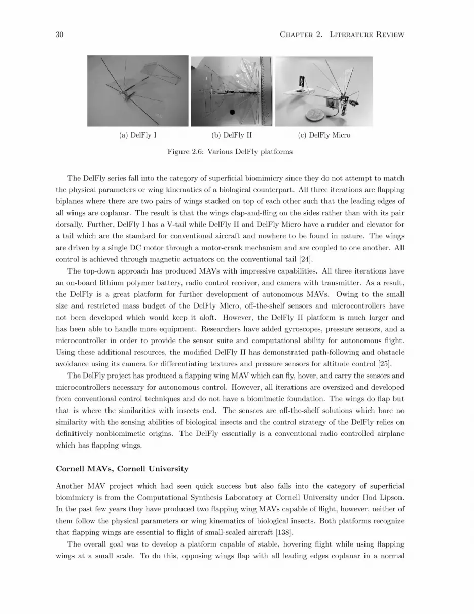
30 Chapter 2. Literature Review
(a) DelFly I (b) DelFly II (c) DelFly Micro
Figure 2.6: Various DelFly platforms
The DelFly series fall into the category of superficial biomimicry since they do not attempt to match
the physical parameters or wing kinematics of a biological counterpart. All three iterations are flapping
biplanes where there are two pairs of wings stacked on top of each other such that the leading edges of
all wings are coplanar. The result is that the wings clap-and-fling on the sides rather than with its pair
dorsally. Further, DelFly I has a V-tail while DelFly II and DelFly Micro have a rudder and elevator for
a tail which are the standard for conventional aircraft and nowhere to be found in nature. The wings
are driven by a single DC motor through a motor-crank mechanism and are coupled to one another. All
control is achieved through magnetic actuators on the conventional tail [24].
The top-down approach has produced MAVs with impressive capabilities. All three iterations have
an on-board lithium polymer battery, radio control receiver, and camera with transmitter. As a result,
the DelFly is a great platform for further development of autonomous MAVs. Owing to the small
size and restricted mass budget of the DelFly Micro, off-the-shelf sensors and microcontrollers have
not been developed which would keep it aloft. However, the DelFly II platform is much larger and
has been able to handle more equipment. Researchers have added gyroscopes, pressure sensors, and a
microcontroller in order to provide the sensor suite and computational ability for autonomous flight.
Using these additional resources, the modified DelFly II has demonstrated path-following and obstacle
avoidance using its camera for differentiating textures and pressure sensors for altitude control [25].
The DelFly project has produced a flapping wing MAV which can fly, hover, and carry the sensors and
microcontrollers necessary for autonomous control. However, all iterations are oversized and developed
from conventional control techniques and do not have a biomimetic foundation. The wings do flap but
that is where the similarities with insects end. The sensors are off-the-shelf solutions which bare no
similarity with the sensing abilities of biological insects and the control strategy of the DelFly relies on
definitively nonbiomimetic origins. The DelFly essentially is a conventional radio controlled airplane
which has flapping wings.
Cornell MAVs, Cornell University
Another MAV project which had seen quick success but also falls into the category of superficial
biomimicry is from the Computational Synthesis Laboratory at Cornell University under Hod Lipson.
In the past few years they have produced two flapping wing MAVs capable of flight, however, neither of
them follow the physical parameters or wing kinematics of biological insects. Both platforms recognize
that flapping wings are essential to flight of small-scaled aircraft [138].
The overall goal was to develop a platform capable of stable, hovering flight while using flapping
wings at a small scale. To do this, opposing wings flap with all leading edges coplanar in a normal

2.3. Microaerial Vehicles 31
(a) Large (b) 3D printed
Figure 2.7: Various Cornell University hovering MAV platforms
hovering fashion. Since all known flapping hovering flight in insects is inherently unstable, a method of
damping the body of the aircraft to retard pitching was developed in order to give the MAV some degree
of passive stability [103]. A comparison of the two Cornell hovering MAV platforms see Figure 2.7 and
Table 2.4.
Table 2.4: Comparison of Cornell University Hovering MAV platforms
Parameter Large 3D PrintedMass 24.2 3.9 gWingspan 45 14.3 cmActuator Motor MotorBattery Life 33 85 sLift-Off Yes Yes
The first, and larger, platform was developed in 2008. An unusual feature was the use of eight
individual wings, four pairs, moving in a plane generating lift using normal hovering with a wingbeat
frequency of 20 Hz. Each wing pair was driven by its own 1.2 g DC motor and the whole system is
powered by two 3.7 V lithium polymer batteries rated at 90 mAh with a mass of 3.1 g each. The wings
were made from a carbon fibre frame with polyester acting as a membrane. The overall system had
a mass of 24.2 g and wingspan of 45 cm. Sails extended above and below the plane of wings which
attempted to impede any body torques from pitching the robot. The sails allowed the system to be
passively stable for flights lasting up to 33 s [138]. No control surfaces were present to control or reorient
the MAV.
The second platform, developed in 2010, was smaller and had made use of 3D printing technology. It
was an evolution of the first platform but with a significant reduction in size. Only four wings, two pairs,
were powered by a single DC motor but are still arranged to flap in the same plane. Unlike the previous
platform, the wings were not assembled from lesser components but rather were fabricated as one piece
using a 3D printer. This had the distinct advantages of being very consistent as well as allowing for
unique and complex designs. For this project, however, the wing design was not selected to follow any
particular biological example. Nonetheless, the wings were observed to twist and camber during stroke
testing which is similar to real insects. To the researchers, however, this was seen as a problem and the
wings were reinforced to act more like flat plates [103]. Sails, identical to the first platform, extended
above and below the frame for passive stability. The overall system had a mass of 3.9 g, wingspan of
14.3 cm, and free flight of 85 s with the on-board batteries. Once again, no control surfaces were present
to control or reorient the MAV.

32 Chapter 2. Literature Review
Both platforms have successfully demonstrated hovering flight. The use of 3D printing for develop-
ment is notable as it demonstrates its usefulness in small-scale fabrication. With the intent, 3D printing
could be used to replicate insect-like wings including the complex vein structures and surface textures.
The lift capabilities demonstrated by these platforms, hovering and being able to carry small loads,
leaves one optimistic for further development. Sensors and microcontrollers can easily be envisioned.
However, the current concepts do not allow direct avenues toward the addition of control surfaces and are
only passively stable. As they are now, the existing designs are very prone to external disturbances such
as wind. These platforms are only loosely biologically inspired, perhaps the investigation of biological
insects could provide some guidance for the control of flapping mechanisms.
CMU MAV, Carnegie Mellon University
Another MAV project has been under development at the NanoRobotics Lab at Carnegie Mellon Uni-
versity under Metin Sitti [91]. What is most notable about this group is that their goal at the outset
was true biomimicry with a small and lightweight piezoelectric-actuated platform. After years of de-
velopment and testing resulted in insufficient lift, the group relaxed their requirements and switched
to kinematic biomimicry by scaling up dimensions and mass to allow for a larger DC motor-actuated
platform.
One of the main goals of this project was to develop an insect-inspired MAV with future control
considerations in mind. Incorporating control concepts very early in the design process was perceived
to be of utmost importance for the long-term success of the project. To truly mimic a flying insect, the
flapping wing MAV should be able to actively stabilize itself during flight. Key design features were to
utilize the passive behaviour of wing pitching and the resonant behaviour of the entire system [65]. All
platforms were tested with off-board power and no batteries were mounted. For a comparison of the two
platforms see Figure 2.8 and Table 2.5.
Table 2.5: Comparison of Carnegie Mellon University hovering MAV platforms
Parameter Piezo-Based Motor-BasedMass 0.7 2.7 gWingspan > 6 > 20 cmActuator Piezo (dual) MotorBattery Life N/A N/A sLift-off No Yes
The first platform relied upon piezoelectric actuation and was first tested in 2010. The design was
based on piezoelectric bending-beam actuators driving a four bar mechanism acting as a transmission
to the wings. The final design used two piezoelectric actuators, one for each wing, thus driving them
independently of one another. As the wings were uncoupled, the flapping amplitude and mean flapping
amplitude allowed for roll and pitch control of the system. The MAV was designed to have a mass of
705 mg, wingspan of over 6 cm, and a wingbeat frequency of 55 Hz [63]. The actuators themselves were
based on the work of Harvard University and had a mass of 130 mg each. Unfortunately, the piezoelectric
actuators were not powerful enough to generate sufficient lift, in fact, only a mean lift force of 1.4 mN
was achieved, which is much less than required to balance the body [64]. In addition, this platform
was externally powered during testing and would need some custom power circuitry for an autonomous
version due to piezoelectrics requiring high voltage to operate (> 100 V). Planning was done for an even

2.3. Microaerial Vehicles 33
smaller version, approximately half the wingspan with a mass of 160 mg. This smaller version yielded
promising simulation results, however, the MAV was not feasible to fabricate and was abandoned.
After attempts at a piezoelectric-based MAV failed, a second platform using DC motors as the
actuation method was then developed. Electromagnetic devices scale poorly, and as a result, the smallest
commercially available DC motors are in the hundreds of milligrams. The motors selected for this
platform were 1.2 g each, with a separate motor per wing. Once again, with a separate actuator moving
each wing, the flapping amplitude and mean flapping amplitude allowed for roll and pitch control of the
system. Unlike other motor-based projects, such as the DelFly, there were no cranks or gears involved.
Instead, each motor was directly connected to a wing spar along with a torsional spring. The motor
was driven by a sinusoidal voltage of up to ±5.5 V with a frequency meant to behave at resonance with
the motor-spring system [62]. Owing to the mass of the motors, the overall size of the MAV had to
be increased to a mass of 2.7 g, wingspan over 20 cm, and a wingbeat frequency of 10 Hz. Using an
off-board power supply and guide wires, this platform was able to achieve lift-off and was measured to
have a 1.4 lift-to-weight ratio [65].
(a) Piezo-Based (b) Motor-Based
Figure 2.8: Various Carnegie Mellon University MAV platforms
Dynamic models of both platforms were developed using a Lagrangian energy approach and used
to simulate flight. The models were based on quasisteady approximations of the aerodynamic forces as
a result of driven wing kinematics. The result was a close prediction of lift generation in the second
platform [65].
Although the first platform aimed to have realistic physical properties and wing kinematics by using
piezoelectric bending-beam actuators, it did not produce nearly enough lift for lift-off. By reverting to
more conventional DC motors as the actuation method and significantly increasing the size and mass
budget, lift-off was achieved but at the sacrifice of no longer being a realistic insect size.
Dragonfly MAV/Cicada MAV, University of Delaware/Purdue University
One of the smallest dragonfly-specific projects was at the University of Delaware under Xinyan Deng.
The initial goal of the project was to design and build a realistic dragonfly MAV by mimicking the
kinematics of their biological counterparts while ignoring realistic physical parameters. As discussed in
Section 2.2.2, this group initially focused on scaled experiments of dragonfly wings. They mounted a
pair of dynamically controlled dragonfly wings, a forewing and hindwing, submerged in a tank of mineral
oil. The wings were 19 cm and 18.5 cm in length for the forewing and hindwing, respectively [68]. By
adjusting the phase difference between the wings they investigated the aerodynamic influence of the
wing-wing interactions.

34 Chapter 2. Literature Review
(a) Dragonfly (b) Cicada (c) EM
Figure 2.9: Various University of Delaware/Purdue University MAV platforms
Table 2.6: Comparison of University of Delaware/Purdue University MAV platforms
Parameter Dragonfly Cicada EMMass > 20.0 2.9 > 5.2 gWingspan > 32 > 10 9− 14 cmActuator Motor Motor ElectromagneticBattery Life N/A N/A N/A sLift-off No No Yes
A robotic dragonfly platform was developed using a 7 g DC motor with a slider-crank mechanism
for each wing pair. The wings were oversized, with a wingspan over 32 cm, and a wingbeat frequency
of 2 Hz. There were no on-board sensors, microcontroller, or battery. All power was tethered from an
off-board source and the prototype was driven open-loop. The mean lift generated was only 93.7 mN
and was much less than what was required to balance the body mass. It did not achieve lift-off [36].
Deng eventually moved to Purdue University before 2011 to continue her research. A new focus was
the development of a cicada platform which used a single pair of wings with a DC motor as the actuator.
The overall platform has a body mass of 2.9 g and a wingspan over 10 cm. The cicada platform has yet
to achieve lift-off [67]. Refer to Figure 2.9 and Table 2.6 for a comparison of the dragonfly and cicada
MAVs.
In 2014, Deng et al. [104] changed actuation methods and began development of an electromagnetic-
based MAV. This two-wing platform utilised a novel method of two electromagnetic actuators, one for
each wing, to generate a flapping motion with no transmission. However, owing to the size of the
actuators (2.6 g each) and massive amounts of power required (24 V tether with 5.76 W of power), this
platform is far from being a feasible biomimetic MAV.
MFI, University of California, Berkeley
A seminal project which began the modern era of MAV research was led by Ronald Fearing of the
Biomimetic Millisystems Lab at the University of California, Berkeley [14]. Beginning in 1998, the first
serious attempt at a biomimetic flapping-wing MAV was the Micromechanical Flying Insect (MFI). The
conditions were ripe to begin an MAV project as the combination of the robotics group led by Fearing
and resident biologists Michael Dickinson and Robert Dudley in UC Berkeley’s biology department.
The collaboration seemed natural as both biologists had decades of experience researching insect flight
between them and had much to contribute to the ideal wing kinematics of the MFI project.
To say that the project goals were ambitious at the time would be an understatement. The template
to be mimicked was a common blowfly, Calliphora [48]. The final MFI goal was specified to have a

2.3. Microaerial Vehicles 35
(a) Partial MFI (b) Artificial ocelli (c) Artificial halteres
Figure 2.10: Highlights of the Micromechanical Flying Insect
total mass less than 100 mg, wingspan of 25 mm, wingbeat frequency of 150 Hz, wing stroke amplitude
of 140°, wing pitch range of ±45°, and deliver 8 mW of mechanical power to the wings [170]. From
the outset, the plan was to include active wing pitch control into the design as well as the independent
control of each of the two wings. The design had the primary components of: thorax, actuators, wings,
and sensors. Piezoelectric actuators combined with a flexible thorax structure were selected as the design
direction [14]. See Figure 2.10a and Table 2.7 for details.
A real insect is a complicated arrangement of muscles and joints inside of an exoskeleton forming
the thorax which has been observed to operate at mechanical resonance during flight [48]. For the
MFI, a complex frame made of carbon fibre trusses acted as an exoskeleton. Inside this frame were
mounted multiple four-bar linkages and spherical joints to move the wings while powered from several
actuators [111,170]. Each wing would have two actuators which would magnify their deflection through
the four-bar mechanisms not only to make the wings flap, but to control the pitch of the wing at will.
This system of the frame with linkages was tuned to resonate at the desired operating frequency of the
MAV. All mechanisms were so small that conventional joints could not be used, so compliant flexure
joints comprised of 12.5 µm thick Polyester to act as rotational hinges [19,111]. In order for the wings to
perform to the desired stroke amplitude range of ±70°, the actuator interface of the four-bar mechanisms
had to be displaced by ±0.25 mm [170].
Table 2.7: Micromechanical Flying Insect properties
Parameter MFIMass 100 mgWingspan 25 mmActuator Piezo (multiple)Battery Life N/A sLift-off No
The actuation method selected for the MFI was piezoelectric bending-beam unimorphs where one
layer was an active piezoceramic while the other was steel to provide some elasticity [111].
Experimentation was also done with elastic extensions to the actuator tip in order to reduce mass
and have greater tip displacement for less blocked force. Another variation was to add a secondary
piezoceramic layer, not to aid in actuation, but to behave as a sensor to provide feedback of the state of the
actuator [19]. Many iterations of piezoelectric actuators were developed, but the final unimorph design
to drive the four-bar mechanisms of the transmission were composed of steel and PZN-PT piezoceramic
[170]. Each actuator had dimensions 5 mm× 1 mm× 0.2 mm where the PZN-PT was 150 µm thick and

36 Chapter 2. Literature Review
the steel was 50 µm thick resulting in a mass of 15 mg. The actuators were expected to generate 7 mW
of power when driven with an excitation voltage of 200 V [48].
The performance of the four-bar mechanisms with these actuators and wings was experimented on
a fixed test-bed. With a feed-forward control signal driving a single wing to a trajectory at a wing-beat
frequency of 150 Hz and stroke amplitude of ±70°, the mean lift over many stroke periods was 506 µN
per wing. This test apparatus demonstrated that the actuated four-bar mechanism design could generate
the necessary lift when on an isolated test bed. However, the entire platform, thorax and all, was too
heavy and the actual natural frequency of the prototype was much lower than expected. Tiny strain
gauges, 1 mm in length, were added to the wing spars in order to measure the force generated. Based on
experimentation, they were shown to be accurate to within ±10 µN [170]. The prototype did not achieve
lift-off. Later attempts to increase lift included a drastic increase in wingbeat frequency, up to 275 Hz,
which required actuators of much larger stiffness. These actuators were enlarged to 100 mg each in order
to double the stiffness. With the increased drive frequency and actuator stiffness, the mean lift over
multiple stroke periods improved to 1400 µN per wing [125]. This demonstrated the benefit of increased
wingbeat frequency on performance; however, the cost was an impossibly large set of actuators. Lift-off
was once again not achieved.
In addition to the lift experiments, the MFI project also did extensive work on dynamic simulations
and sensor development. With the long-term goal of autonomous flight, some sensing capabilities would
be necessary in order to provide feedback to a future controller for flight stabilization. In keeping with
the biomimetic approach, several biologically inspired sensors for navigation and stabilization were put
into development. These sensors both had to match similar performance specifications of their biological
counterparts while also meeting the strict low mass and low power budgets allotted [168]. The first
sensor was based on ocelli which are light sensitive photosensors located on the head of some flying
insects. Multiple ocelli can be found on the upper surface of the insect and are used to detect light from
the sky. They are believed to aid in horizontal stabilization, and in some species, for migratory purposes
by following areas of high light intensity such as the sun. For the MFI project, researchers worked to
construct a small, multifaceted sensor which housed four photodiodes angled outward in four directions.
In this way, the individual photodiodes could be used to detect when the MAV was not oriented in an
upright position if one (or more) measures only small amounts of light intensity. The final sensor had
dimensions 5 mm × 5 mm × 5 mm and a mass of 150 mg [168]. Although functional, it was still much
too large and heavy to be used for flight. The artificial ocelli constructed for the MFI project can be
seen in Figure 2.10b. A second sensor was based on halteres, commonly found on two-winged insects
such as houseflies. Halteres, as mentioned previously, are a pair of knobby protrusions, one on each
side of the thorax, which are used to measure body rotations by acting as gyroscopes. It is believed
that they once were a second pair of wings which have, over time, evolved into these small sensory
organs. The halteres vibrate 180° out of phase with the wings and are angled to not be perpendicular
with the body such that they are not coplanar to each other and can thus be sensitive to rotations in
all three dimensions [168]. The MFI project developed artificial halteres which were 5.5 mm in length
and had a mass of 10 mg each while being driven to vibration by piezoelectric actuators. The Coriolis
effect influenced the halteres during changes in direction and was measured by small strain gauges at
the base of the halteres. Through experimentation, these artificial halteres demonstrated remarkable
accuracy when compared to simulation [169]. The halteres constructed for the MFI project can be seen
in Figure 2.10c. Finally, houselfies have relatively poor vision but are able to respond to changes in

2.3. Microaerial Vehicles 37
contrast. The MFI group began experimenting with optic flow arrays which consisted of a low resolution
camera. In this way, the sensor could provide some feedback for significant changes in the environment
as a form of visual stimulus [168].
Strict requirements, great attention to current insect flight research, and creative use of technology
allowed the MFI project to lay the foundation for all current MAV projects. Unfortunately, the MFI
never did achieve lift-off and the project appears to have been retired in 2008. However, the MFI project
proved to be the genesis of all major flapping-wing MAV projects across the United States today. Metin
Sitti of Carnegie Mellon University, Xinyan Deng of Purdue University, and Robert Wood of Harvard
University all began their MAV research while working on the MFI project at the University of California,
Berkeley.
The Biomimetic Millisystems Lab at UC Berkeley has been home to a number of other microrobotic
projects. DASH (dynamic autonomous sprawled hexapod) was a six-legged walker which was modified to
have flapping wings mounted upon it to experiment with wing-assisted running and discovered potential
implications for avian flight evolution [96]. BOLT (bipedal ornithopter for locomotion transitioning)
was a lightweight bipedal ornithopter which transitions between terrestrial and aerial locomotion [97].
VelociRoACH implemented an aerodynamic rotational damper to demonstrate that rotational dynamics
could improve stability while running [58]. Multiple other MAV projects involving ornithopters with
larger wingspans have since expanded on the findings of the MFI project [105].
MicroFly/RoboBee, Harvard University
Without question, the most successful true biomimetic flapping-wing MAV project has been under
Robert Wood of the Harvard Microrobotics Lab at Harvard University [60]. Under Wood, this MAV
project evolved from UC Berkeley’s MFI project beginning in the mid 2000s [160]. This group is
considered leaders in the field because it was the first to demonstrate that a partial biomimetic MAV
could achieve lift-off, which it did in 2007 [159]. The project has had two phases: the first being the
Harvard Microrobotic Fly (HMF) which was modelled after Diptera and flew in 2007, the second was
the RoboBee which was modelled after a honeybee first appeared in 2012 [133]. The HMF had a single
piezoelectric actuator which drove both wings whereas the RoboBee design had two separate piezoelectric
actuators which drive each wing independently [133]. The direct impact of this project on the field has
been monumental. An influential demonstration of design, fabrication, and implementation of modern
technologies are just a few examples of their contributions. The key characteristics of insect flight which
they had implemented in their designs are the mechanical advantage insects use in their thoracic muscles
and joints to amplify the wing stroke, tuning the system to operate at resonance, and that some aspects
of insect wing trajectories are mechanically hard-coded during flight [161].
Biomimetic systems must make use of modern technology in order to meet, and perhaps exceed,
the capabilities of their biological counterparts. Insect flight muscle has been measured to have power
densities around 80− 83 W/kg, but piezoceramics have been shown to have power densities upwards of
400 W/kg. By taking advantage of the performance of this piezoelectric material, this becomes one of
the first microrobotic systems which has the potential to exceed that of nature [159,161]. Both Dipteran
insects and honeybees use direct flight muscles attached to their exoskeletons. A push-pull method of the
muscles attached to a network of joints behaves kinematically like a four-bar mechanism [158]. The HMF
and RoboBee use carbon fibre beams with flexures of polymide film between them to create comparable
four-bar mechanisms while keeping mass to a minimum. The four-bar amplifies the near linear input of

38 Chapter 2. Literature Review
(a) Harvard HMF Model (b) Harvard HMF Realization (c) Harvard RoboBee
Figure 2.11: Various Harvard University MAV platforms
the piezoelectric bending-beam actuator into an angular output to drive the wings [133]. By driving the
actuator at resonance, the stroke amplitude was magnified significantly [81].
Table 2.8: Comparison of Harvard University MAV platforms
Parameter HMF RoboBeeMass 60 80 mgWingspan 30 30 mmActuator Piezo (single) Piezo (dual)Battery Life N/A N/A sLift-off Yes Yes
The wings were designed to match the size and shape of the insects they were mimicking. The
primary goal was to keep the wings rigid for the expected loading conditions of aerodynamic force at
the desired wingbeat frequency. Early iterations had wings made of polyester with simplified carbon
fibre spars while later iterations had 3D printed wings with more complex vein structures. Each wing
measured 15 mm in length and had a mass of 400 µg. The wings would pitch passively based on a
polymide film hinge which could be selected to adhere the maximum angle desired [161]. Early wing
kinematics allowed for passive wing pitching only and stroke plane deviation was restricted as it was
the easiest to fabricate. Even with these simplifications, however, the wing kinematics resembled that
of real insects during hover conditions [81].
The first platform was the Harvard Microrobotic Fly (HMF) which was the first true biomimetic
partial MAV to lift-off. Partial, in this case, means that it was only a frame with an actuator. To that
point, no sensors, microcontroller, or on-board power supply was present. The basic design was to mimic
the physical characteristics of a Dipteran fly and had a total wingspan of 30 mm, body mass of 60 mg, and
wingbeat frequency of 250 Hz [158–160]. Fabricated mostly out of carbon fibre with polymide film joints,
the single actuator was a custom designed piezoelectric bending-beam actuator. The actuator itself was
composed of PZT-5H piezoceramic and had a mass of 40 mg with a tip deflection of ±400 µm [161]. The
tip of the actuator interfaced with the rest of the system through a transmission which amplified the
translational input into a wing rotation. A bidirectional force of the actuator resulted in the up/down
motion of the wings. The wings were simple replications of Dipteran wings using carbon fibre spars and
1.5 µm polyester for a wing membrane [159]. Through the transmission, all wing motion was restricted
to a constant stroke plane [81]. The Harvard group recognized that resonance would have to play a key
roll in order to succeed. Using an energy modelling approach, the resonant frequency of the system was
approximated [158]. Unfortunately, the calculated resonant frequency of the design was to meant to
match the performance of a real fly, being 250 Hz, whereas the actual observed performance of the HMF

2.3. Microaerial Vehicles 39
was closer to 110 Hz [161]. The HMF still was able to give the desired stroke amplitude and generated
sufficient force to lift-off. In fact, the average lift was 1.14 mN producing a lift-to-weight ratio near
2 [158]. Using high-speed video to observe the wing kinematics of the passively pitching wings, the wing
trajectory appeared to be nearly identical to biological insects. As there was no method of passive or
active stabilization of the body in the early stages of the project, the entire MAV had to be restricted
to guide wires allowing only one dimensional movement. Several years after first achieving lift-off, some
attempts at active stabilization were done by adding two small piezoelectric actuators on the frame to
asymmetrically alter the wing kinematics. The result was adjusting the mean stroke amplitude on one
side to be larger than the other, thus instigating roll [51]. Although sound in principle, this modification
proved too costly in mass and was ineffective for in-flight stabilization.
The second platform was the RoboBee which has also been able to achieve lift-off. This version
was modelled after the common honeybee but retained somewhat similar design requirements to the
HMF with the exception of a reduced wingbeat frequency. A major source of funding for this project
has been the National Science Foundation with the intent of swarms of artificial pollinators to mitigate
crop losses owing to large quantities of honeybee deaths [92]. The actual platform has a wingspan of
30 mm, body mass of 80 mg, and wingbeat frequency of 120 Hz [81]. The primary difference between
the RoboBee and its predecessor, the HMF, was in actuation. The RoboBee utilised two piezoelectric
actuators which independently drove the wings. Now each wing could have any desired stroke amplitude
and mean stroke amplitude independent from one another, thus allowing pitch and roll control more
reliably. The variation in output thrust was achieved through modulation of these amplitudes. Once
again, however, the wings remained restricted to a specific stroke plane [81]. The platform itself, with
nothing but the frame, wings, and actuators were able to achieve lift-off with a maximum mean lift
force of 1.3 mN. There was no on-board power supply and the necessary 19 mW of power was supplied
through a tether. Even with the careful laser-cutting fabrication process, imperfections in construction
still permeated the prototypes. Any asymmetry in the flapping mechanism would cause the robot to
deviate from the vertical trajectory [95]. Robust control methods were necessary for free flight. Using a
network of eight high-speed cameras located in the surrounding environment to provide feedback to an
off-board controller, the RoboBee was fed drive signals through an umbilical in order to perform stable
altitude and attitude in flight for over 20 s [81]. It was then demonstrated to be capable of executing
simple pitching and rolling manoeuvres. The RoboBee had proven to be an at-scale platform which
could fly and be stabilized. All that was missing were the appropriate on-board sensors, microcontroller,
and power supply.
(a) Before “pop-up” (b) After “pop-up”
Figure 2.12: Harvard “pop-up” monolithic assembly method [124]
The size of the prototypes proved to bring about special challenges. With a scale between mi-
crons and centimetres, the fabrication method required to construct these prototypes were too large for

40 Chapter 2. Literature Review
MEMS methods and too small for conventional assembly techniques. In between these two realms is
the mesoscale which had no rigorously established fabrication procedures beforehand. A new method
dubbed “Smart Composite Materials” (SCM) was developed which layered materials, cut them to size
with a laser, added epoxy, applied compression, cured in an oven, and assembled the components [163].
This method made it easy to construct complex structures with rigid components combined with the
flexible joints in a consistent manner. In addition, a “pop-up” assembly method had proven to drastically
reduce variation. First, all layers of carbon fibre, adhesive and flexible joint layers were combined into
a monolithic structure. Then the appropriate patterns were cut using a laser similar to printed circuit
board manufacturing methods. With careful design, the assembly could “pop-up” into the final three-
dimensional configuration and be fixed in-plane using adhesives or a soldering process. This method
allowed topologically complex designs to be easily aligned and assembled [124]. See Figure 2.12 for an
example of this method with the HMF. The long-term goal of the “pop-up” method is to support quick
and easy manufacturing of mesoscale devices at industrial pace.
The Harvard group has done a lot of work applying existing piezoelectric actuation technology to
MAV applications. Continuing the work of Smits [121], the group at Harvard has experimented with
material selection, composite fabrication methods, and different drive configurations beneficial to micro-
robotics [157]. More detailed, however, is their attention to the push/pull performance of the actuator
at resonance to better mimic the behaviour of real insect flight muscle [81]. Essential to the future
autonomous flight of the RoboBee is the ability to provide on-board power. Piezoelectrics are unique
in that they are low power devices which require low current but high voltage in order to operate. Ac-
knowledging that the most likely power supply to have the most energy density at the low masses desired
are lithium polymer batteries with low output voltages around 3.7 V, a method of boosting the voltage
up above 200 V was necessary. Karpelson [76], a member of the Harvard Microrobotics Lab, developed
multiple ultralight, high-voltage power circuits for DC-DC amplification. The result was a 20 mg circuit
capable of boosting a 5 V signal up to 200 V while still maintaining 70 mW of power output which is
more than enough to power the drive actuators and multiple sensors of the RoboBee. The circuit itself
consisted of two stages, a tapped inductor to generate the high voltage and a switching amplifier in order
to generate a sinusoidal drive signal.
The Harvard group attempted to simulate the dynamic behaviour of the wings using blade-element
models. Detailed equations of motion were derived for the rotational dynamics of the wings leading
to aerodynamic force and moment estimates. They were unable to reproduce the unsteady flow fea-
tures, such as wake capture, as their method was quasisteady and only estimated forces based only on
instantaneous forces [156]. They were unsure as to the significance of muscle involvement of wing flip
(pronation or supination) and to whether they could actively control the rotation or merely provide
adjustments [156, 161]. What was agreed upon was that the passive rotation of wings during flapping
flight was both effective and the easiest to recreate in a robotic insect. They were one of the first groups
to use a simple wing hinge to passively allow a rigid wing to pitch due to aerodynamic damping [156]. In
the basic Harvard platforms, the wing hinges were constructed of thin-film polymide acting as rotational
springs between the carbon fibre transmission and leading edge of the wing. The stiffness of these hinges
were determined by modelling the joints as wide, thin, and short cantilevers [163]. If the hinge was too
stiff, the wing would under-rotate. If the hinge was not stiff enough, the wing would over-rotate and
tend to flutter during normal operation. More recently, the group has developed a method of active
pitch control of the wings during flight. A differential, controlled by a single piezoelectric actuator, can

2.3. Microaerial Vehicles 41
adjust the resting orientation of the wing hinge of each wing, thus biasing the wing pitch without having
an impact on stroke plane amplitude [133]. If retrofitted with this differential, the RoboBee could have
independent wing amplitude control and wing pitch control giving it even more control surfaces to aid
in flight correction.
Figure 2.13: Active control of the wing hinge rest position of the Harvard RoboBee [133]
With two MAV platforms capable of lift-off and the ability to control themselves, the Harvard group
has been working to develop biomimetic sensors to provide on-board feedback. For the HMF, a biolog-
ically inspired optical flow sensor matching the very low visual capabilities of flies was fabricated and
tested. The 4× 32 pixel array was very low resolution, but it did allow for changes in contrast, and thus
movement, to be observed [40].
Another sensor was Harvard’s attempt at recreating ocelli. Similar to that of UC Berkeley, these
sensors are meant to measure the light intensity of the sky to maintain orientation with the horizon.
They had shown that an angular velocity estimate is all that is needed to stabilize the upright orientation
of the MAV. The final sensor had dimensions 4.0 mm × 4.0 mm × 3.3 mm and a mass of 25 mg [54].
Using off-board power and computational processing, control signals were sent to the MAV using the
ocelli sensor as the sole source of feedback information to successfully keep it vertical while hovering.
A third sensor used to stabilize the attitude of the RoboBee is a MEMS-based gyroscope. Using an
off-the-shelf inertial measurement unit (MPU9150 from Invensense), which has a mass of 40 mg, was
mounted to the RoboBee platform. This sensor had a 3-axis accelerometer, 3-axis gyroscope, and a
3-axis magnetometer. Adding to this the high bandwidth capability of 1 kHz, this was one of the first
MEMS sensors lightweight enough to be carried on-board an MAV with such broad functionality. Using
off-board computational processing and tethered power, the RoboBee with this sensor demonstrated
attitude stabilization for 2 to 5 s while hovering while a camera system provided feedback solely for
positional feedback [53].
The progress made by the Harvard Microrobotics Lab is impressive. They have the capability to
fabricate a prototype from scratch to flight-ready in less than one week [159]. Significant obstacles
remain, however. Components such as sensors, power source, and microcontroller must be made small
enough and yet remain effective for the autonomous flight of MAVs to be possible. Each prototype, even
with rigorous fabrication methods, still have slight asymmetries which need to be overcome by robust
control methods.

42 Chapter 2. Literature Review
2.4 Piezoelectric Actuation
In the quest to recreate insect flight, one of the most crucial components is the method of actuation.
The actuator dictates the entirety of the design of an MAV from the overall dimensions to the power
supply selection. What is paramount is that the actuator must provide the minimum amount of energy
to power the wings to generate lift. As discussed in Section 2.1.4, insect flight muscle has a power density
of 80 to 83 W/kg [159]. For an MAV equivalence, this could be considered the required power density
of the actuator plus the battery source since the insect flight muscle alone accounts for both of those
responsibilities although in engineering this can be flexible.
When the characteristic dimension of an MAV is measured in millimetres, conventional actuation
methods such as electromagnetic motors become ineffective due to scaling issues. Although powerful and
easily capable of high bandwidth output, existing DC motors are simply too heavy for true biomimetic
applications. If mass requirements were relaxed, however, DC motors would be a very attractive option.
Another possible option is shape memory alloys (SMAs), although scalable to any size, they do not
fair well at the high bandwidth operation regime of insect flight due to their high current draw and
undesirable tendency to overheat. Piezoelectrics are a welcomed alternative; they tend to be scalable,
capable of high bandwidth operation, and do not tend to suffer from overheating issues [73].
Piezoelectricity is process of electromechanical interaction inherent in certain materials. The study
of piezoelectric materials is complex in that it involves crystal physics, material science, and electrome-
chanical interaction. While attempting to model such phenomena requires the combination of mechanics,
electromagnetic theory, and thermodynamics [71].
One of the most successful insect-inspired MAV projects to date has utilised piezoelectric bending-
beam actuators, namely, Harvard University’s RoboBee. Citing the high power density of 400 W/kg
for piezoelectrics as the primary reason for their selection, it appears that this is the best choice for
true biomimetic MAV applications at present [159]. Obstacles to overcome include the necessarily high
voltage requirement to get piezoelectric actuators to perform as well as finding the optimal configuration
for a particular application.
Piezoelectric bending-beams are not just limited to the field of microrobotics. The inherent properties
of piezoelectric materials make them useful as both actuators and sensors. They can provide feedback
about their environment just as well as they can interact with it. Piezoelectric materials have a tendency
of behaving somewhat like capacitors and, given the right conditions, could be used to extract energy
from their surrounding environment to be collected and stored is energy harvesters [70,136].
2.4.1 The Piezoelectric Effect
The word piezoelectricity derives from the Greek words piezein, meaning “to press,” and elektron, mean-
ing “amber,” which was the name the ancient Greeks gave to the mysterious attractive force observed
when some materials were rubbed. The category of piezoelectric materials are special in that a defor-
mation caused by an external pressure will result in the production of an electric field, and conversely,
the application of an electric field will result in a deformation. These are called the direct piezoelectric
effect and the inverse piezoelectric effect, respectively [18]. In general, sensors make use of the former
while actuators make use of the latter. A piezoelectric material serves three primary purposes: first as a
capacitor for storing electrical energy, second as a motor for converting electrical energy into mechanical
energy, and third as a generator for converting mechanical energy into electrical energy [84].

2.4. Piezoelectric Actuation 43
(a) Centrosymmetric (b) Noncentrosymmetric
Figure 2.14: Piezoelectric crystal structure (a) above and (b) below the Curie temperature [10]
Both the direct and inverse piezoelectric effect are manifestations of same fundamental property of the
crystal structure [71]. All crystals fall into 32 classes, 20 of which demonstrate piezoelectric properties
and 12 which do not. What determines the piezoelectricity of a crystal is determined by its centre
symmetry [84]. Materials which show piezoelectric behaviour have tetragonal crystal structures which
do not have a symmetric centre, and are therefore called noncentrosymmetric as seen in Figure 2.14. As a
result, the positive and negative ions of the crystal lattice lead to the phenomenon of polarization. When
a piezoelectric crystal is observed from an outside point of view with no applied stresses or potentials,
the entire crystal is electrically neutral. In order for the piezoelectric effect to occur, polar axes must
exist within the crystal structure. A combination of uniform stresses produce a separation of the centres
of gravity of the positive and negative charges and induce a dipole moment which is necessary for the
production of polarization by stresses [84]. This means that the distribution of the electric charge within
the chemical bonds exist in a dipole moment. This is the measure of the positive and negative charges
and their separation within a charge system and also defines the polarization direction of the system [10].
The electrical polarization caused by the dipole moment within a crystal cell can be represented
by a polarization vector. The material can have multiple regions with different polarization directions
best represented by a vector field. Each region is a collection of aligned dipoles which naturally occur in
random orientations to one another as seen in Figure 2.15a. In order to make piezoelectric materials useful
for engineering purposes, the various regions can all be aligned into a single polarization direction through
a process called “poling.” This is done by raising the temperature of a piezoelectric material above its
Curie temperature, then the material consists of simple cubic crystal structures and is temporarily
centrosymmetric. In this state, the various regions no longer have dipoles present and are essentially
free to reorient themselves. The application of an external electric field causes all regions to align. As the
temperature is reduced back below the Curie temperature, these regions become locked in parallel. This
process can be seen in Figure 2.15b to Figure 2.15c. The material again becomes noncentrosymmetric
but now all of the dipoles throughout become aligned and the material is then said to be macroscopically
polarized [10, 12]. This process is used in the manufacturing of piezoceramics such as the popular lead
zirconate titanate (PZT) family.
When an electric field is applied to a macroscopically polarized piezoelectric material in the same
direction as the polarization direction, the material uniformly responds by expanding in that direction

44 Chapter 2. Literature Review
(a) Before polarization (b) During polarization (c) After polarization
Figure 2.15: Comparison of piezoelectric crystal regions throughout the poling process
while also contracting in the perpendicular directions. If the electric field is applied in the opposite
direction of polarization, the material will contract in that direction while expanding in the perpendicular
directions. Piezoelectricity is a linear effect and the reversal of the applied electric field results in the
reverse mechanical effect [12]. An applied electric field can cause the material to undergo expansions and
compressions dependent on the orientation of the monocrystalline structure resulting from polarization.
2.4.2 History of Piezoelectricity
Knowledge of piezoelectricity’s existence has been around for millennia, however, it first became known
to modern Europe when Dutch merchants brought tourmaline crystals from Ceylon, now Sri Lanka, in
the 1700s [18]. Piezoelectricity is closely tied to the phenomenon of pyroelectricity which is the electrical
behaviour of a crystal due to thermal effects. The official discovery of the piezoelectric effect has been
attributed to the French physicists Pierre & Jacques Curie in 1880. The Curie brothers intentionally
set out to observe piezoelectricity as they hypothesized of its existence due to their previous experience
with pyroelectric materials [18]. They observed that select materials, such as tourmaline, respond to
an applied mechanical stress by the production of electric surface charges which led to the discovery of
the direct piezoelectric effect [84]. In fact, they noticed that deformation in certain directions caused
consistent and proportional electrical surface charges and were quick to develop a relationship between
the application direction of pressure and resulting charge [12]. Other naturally occurring crystals were
found to demonstrate piezoelectric behaviour in early investigations, these include: zinc blende, cane
sugar, topaz, Rochelle salt, and quartz to name a few [85]. The inverse effect was not immediately
obvious to them, however, Gabriel Lippman the following year hypothesized its existence through his
theoretical work which was promptly confirmed by the Curie brothers. The discovery of piezoelectricity
earned the Curie brothers the Plante prize in 1895.
The piezoelectric effect remained only a novelty for decades. It was only with the outbreak of war did
practical applications begin to surface. During World War I, Paul Langevin in Paris requested that the
French government invest in efforts to devise some way of detecting submarines. He conceived of the idea
of using quartz glued between metal plates could act as emitters when excited by a voltage potential.
When applied, the crystals expanded and sent out a longitudinal wave which could also be detected
using the same method in reverse [84]. These signals would be picked up by transducers from surface
ships [85]. The resulting echoes could be used to locate immersed objects such as submarines as well as
exploring the depths of the ocean bottom. Langevin is often credited for the creation of ultrasonics and
the use of acoustic waves [18].

2.4. Piezoelectric Actuation 45
With the successful application of piezoelectrics, the end of the war led to many peacetime applica-
tions. Early in the 1920s, quartz was used to create oscillators and filters, Rochelle salt in low-frequency
transducers, and tourmaline for measuring hydrostatic pressures [84]. Quartz crystals became widely
used as resonators for frequency control and time-keeping by using a vibrating quartz plate or ring to
replace the conventional swinging pendulum [18]. Starting in the 1930s, C.B. Sawyer worked on crystal
growth as well as crystal element fabrication as part of the quest to uncover materials with even greater
piezoelectric coupling [72]. Other applications included: microphones, telephone speakers and receivers,
phonograph pick-ups, all of which were superior to their electromagnetic predecessors [12,18].
One piezoelectric pioneer was Walter G. Cady of Wesleyan University. His life’s work took root
while contributing to the antisubmarine task group in 1917 on underwater signalling and detection [72].
After realising the promise of piezoelectrics, Cady collaborated with General Electric in 1921 on quartz
resonators. He showed that quartz crystals could be used as control oscillators with the prominent
application being the frequency control of military communication equipment [84]. He developed the first
piezoelectric resonators using mechanical resonance as the foundation of oscillators and filters. His work
profoundly influenced radio transmitter technology and frequency control applications thereafter [18].
Another pioneer was Warren P. Mason of Bell Telephone Laboratories. Mason was the first to
establish the interrelation of dielectric, piezoelectric, and elastic constants in Rochelle salt and materials
of high piezoelectric coupling [72]. Bell Labs did significant research into piezoelectric crystals and their
application to communication equipment, filters, oscillators, and electromechanical transducers is felt to
this day [84]. During the war effort in World War II, communication filters required very large crystals
(> 5 cm), as supply became short during and after the war and alternatives were needed [84]. Bell
Labs developed multiple artificial piezoelectric materials with high piezoelectric coupling properties such
as ADP (ammonium dihydrogen phosphate), DKT (dipotassium tartrate), and EDT (ethylene diamine
tartrate). The latter of which had quickly replaced quartz in telephone filters when quartz was difficult
to obtain in large quantities [84]. As Mason’s career was coming to an end, others at Bell Labs continued
to contribute to piezoelectrics such as Harry F. Tiersten with his primary work being on the dynamics
of piezoelectric plates [135].
At the end of World War II, the rapid increase in interest for piezoelectrics led to two seminal texts
on the subject: Piezoelectricity by Cady in 1946 [18] and Piezoelectric Crystals and Their Application to
Ultrasonics by Mason in 1950 [84]. These are often viewed as the foundation of the field of piezoelectricity
today. The increase in interest also necessitated the need for conformity such that the major contributors
could align with respect to notation. The Standards on Piezoelectric Crystals of 1949 was written by
a Piezoelectric Committee formed by the Institute of Radio Engineers, chaired by Cady and heavily
influenced by Mason [1]. Since then, standards have been updated several times leading to the most
recent in 1987 by the IEEE [2], this time heavily influenced by Tiersten.
Today, most piezoelectrics in use are artificial with ever-increasing performance well exceeding those
found in nature. One of those has been the family of piezoceramics such as lead zirconate titanate,
or PZT [80]. The process in producing these polycystalline ceramics ensure that very high coupling
coefficients result through a process which aligns the polarization regions such that they work uniformly.
Most of the older crystal-based transducers have since been replaced by these piezoceramics which are
much more effective and easier to produce en masse [85]. Today, piezoelectrics are found in most
electronic devices, medical equipment, and so much more as they make great sensors due to their small-
size, sensitivity, and lack of a need for excitation.

46 Chapter 2. Literature Review
2.4.3 Linear Theory of Piezoelectricity
In order to make use of piezoelectric materials, the fundamental principles behind the piezoelectric effect
must be described mathematically. This Section summarizes the contents of the IEEE Standards of
Piezoelectricity [2] as well as the work of Ballas [10], Cady [18], Mason [84], and Tiersten [135].
A linear relationship between the mechanical and electrical behaviour of piezoelectrics has been
well documented. The linear theory of piezoelectricity couples the mechanical behaviour using linear
elastic equations with the electrical behaviour using the charge equations of electrostatics. This yields a
relationship via a collection of piezoelectric constants. It is important to note, however, that the electric
variables are not purely static, but quasistatic, yet can be approximated as such for most uses.
Piezoelectric Thermodynamic Functions
Piezoelectricity is process of electromechanical interaction and energy conversion. The piezoelectric
constitutive equations are the basis for many piezoelectric bending-beam models for use in engineering
applications. However, the origins of these equations are rooted in thermodynamics.
A thermodynamic potential is a scalar quantity which is used to represent the thermodynamic state
of a system. The four classical thermodynamic potentials are: internal energy (U), enthalpy (H),
Helmholtz free energy (A), and Gibbs free energy (G). Each of these are comprised of four variables
describing the system, namely: pressure (p), volume (V ), temperature (Θ), and entropy (σ). Of these
variables, two are independent and two are dependent. These are summarized in Table 2.9 as outlined
by the International Union of Pure and Applied Chemistry (IUPAC) [5].
Table 2.9: List of classic thermodynamic potentials [5]
Potential Function Differential Indep. Var.Internal Energy U = Θσ − pV dU = Θdσ − pdV U(σ, V )Enthalpy H = U + pV dH = Θdσ + V dp H(σ, p)Helmholtz Free Energy A = U −Θσ dA = −σdΘ− pdV A(Θ, V )Gibbs Free Energy G = U −Θσ + pV dG = −σdΘ + V dp G(Θ, p)
The internal energy is the capacity of the system to do work and release heat. In general, this
excludes the kinetic energy of motion of the system and the potential energy due to external force
fields (electrostatic/electromagnetic/etc.). It can be changed by heating the system or doing work on it.
Usually this is a preferred expression of a system under constant volume and entropy. From the 1st and
2nd Laws of Thermodynamics,
dU = δQ+ δW (2.2)
where dU is the exact differential of the internal energy, δQ is the infinitesimal differential of heat
transfer, and δW is the infinitesimal differential of work done. For a reversible process, the 2nd Law
implies that δQ = Θdσ. Also, work can be represented as δW = −pdV where the negative signifies
energy flow from system to the surroundings. Now (2.2) becomes
dU = Θdσ − pdV (2.3)
where, as stated earlier, the internal energy is a function of the independent variables entropy and
volume.

2.4. Piezoelectric Actuation 47
The enthalpy is the capacity of the system to do nonmechanical work and release heat. Usually this is
a preferred expression of a system under constant pressure and entropy. Starting with (2.3) and adding
d(pV ) to both sides
dU + d(pV ) =Θdσ − pdV + d(pV )
d(U + pV ) =Θdσ − pdV + V dp+ pdV
dH =Θdσ + V dp
(2.4)
where H = U + pV is a function of the independent variables entropy and pressure.
The Helmholtz free energy is the capacity of the system to do work. Usually this is a preferred
expression of a system under constant volume and temperature. Starting with (2.3) and subtracting
d(Θσ) from both sides
dU − d(Θσ) =Θdσ − pdV − d(Θσ)
d(U −Θσ) =Θdσ − pdV − σdΘ−Θdσ
dA =− σdΘ− pdV
(2.5)
where A = U −Θσ is a function of the independent variables temperature and volume.
The Gibbs free energy is the capacity of the system to do nonmechanical work. Usually this is a
preferred expression of a system under constant pressure and temperature. Starting with (2.5) and
adding d(pV ) to both sides
dA+ d(pV ) =− σdΘ− pdV + d(pV )
d(A+ pV ) =− σdΘ− pdV + V dp+ pdV
dG =− σdΘ + V dp
(2.6)
where G = A+ pV is a function of the independent variables temperature and pressure.
In his 1946 text, Cady [18] discussed the new piezoelectric formulation as an analogous represen-
tation to the well-known thermodynamic expressions discussed. In this way, internal energy, enthalpy,
Helmholtz free energy, and Gibbs free energy can be redefined in terms of strain, stress, electric dis-
placement, and electric field. Here, the work done is not in terms of pressure-volume but in stress-strain
and electric displacement-electric field relationships. In order to maintain the full set of combinations of
independent variables additional thermodynamic functions are defined. These are: elastic enthalpy H1,
electric enthalpy H2, elastic Gibbs free energy G1, and electric Gibbs free energy G2.
The foundational thermodynamic function is internal energy of a volume, U , now also defined [84] as
U = TijSij + EkDk + Θσ
where Tij is the stress tensor, Sij is the strain tensor, Ek the electric field, Dk the electric displacement,
Θ the temperature, and σ the entropy of that volume. The three terms represent each of the three
variable pairs, as listed in Table 2.10.
Using the internal energy as a starting point, all eight relevant thermodynamic functions can be
collected and are listed in Table 2.11. When dealing with electromechanically coupled systems, they can
be broken down into two categories: adiabatic and isothermal. The former where entropy is assumed

48 Chapter 2. Literature Review
Table 2.10: List of intensive and extensive variables
Intensive ExtensiveTij ←→ SijEk ←→ Dk
Θ ←→ σ
constant and the latter when temperature is assumed constant [71]. If thermal effects are ignored (or
assumed constant), the eight equations can be reduced to four.
Table 2.11: List of thermodynamic functions [84]
Potential Function Indep. Var.Internal Energy U = TijSij + EkDk + Θσ U(Sij , Dk, σ)Enthalpy H = U − TijSij − EkDk H(Tij , Ek, σ)Elastic Enthalpy H1 = U − TijSij H1(Tij , Dk, σ)Electric Enthalpy H2 = U − EkDk H2(Sij , Ek, σ)Helmholtz Free Energy A = U −Θσ A(Sij , Dk,Θ)Gibbs Free Energy G = U − TijSij − EkDk −Θσ G(Tij , Ek,Θ)Elastic Gibbs Free Energy G1 = U − TijSij −Θσ G1(Tij , Dk,Θ)Electric Gibbs Free Energy G2 = U − EkDk −Θσ G2(Sij , Ek,Θ)
Each of the eight thermodynamic functions can lead to a set of three constitutive equations (eight
groups of three equations where the three dependent variables are functions of the three independent
variables). However, if we ignore pyroelectric effects, or that at least one of temperature or entropy will
always be zero, then there are four pairs of constitutive equations (four pairs of two equations where
the two dependent variables are functions of the two independent variables). These reduced constitutive
equations are listed in Table 2.12 [2, 71].
Table 2.12: List of constitutive equation pairs [71,84]
Indep. Var. Const. Equations Thermodynamic FunctionSij , Dk Tij = cDijklSkl − hkijDk U = 1
2cDijklSijSkl − hkijDkSij + 1
2βSijDiDj
Ei = −hiklSkl + βSikDk
Tij , Ek Sij = sEijklTkl + dkijEk H = − 12sEijklTijTkl − dkijEkTij − 1
2εTijEiEj
Di = diklTkl + εTikEkTij , Dk Sij = sDijklTkl + gkijDk H1 = − 1
2sDijklTijTkl − gkijDkTij + 1
2βTijDiDj
Ei = −giklTkl + βTikDk
Sij , Ek Tij = cEijklSkl − ekijEk H2 = 12cEijklSijSkl − ekijEkSij − 1
2εSijEiEj
Di = eiklSkl + εSikEk
Mechanical Considerations
By looking at small deformation theory, where an infinitesimal volume is assumed, several important
equations regarding mechanical relationships are defined. First, the displacement ui is defined to be
in the three-dimensional Cartesian frame (where i,j = 1, 2, 3). From this, the spatial gradient can be
defined as
ui,j =∂ui∂xj
= Sij + ωij

2.4. Piezoelectric Actuation 49
which is a second rank tensor with nine components and can be broken down into symmetric, Sij , and
nonsymmetric, ωij , parts where
Sij =1
2(ui,j + uj,i) and ωij =
1
2(uj,i − ui,j)
If the nonsymmetric portion, the rigid rotation, is ignored then the spatial gradient can be approximated
to be
ui,j ≈ Sij (2.7)
which is known as the strain tensor.
The surface traction (ti) represents the mechanical interaction between two components on the surface
(S) of the material. Also important is the stress tensor (Tij), defined as
ti = niTij (2.8)
where ni represents the outward unit normal from the surface where the traction acts. A relationship
which will be useful later is found by using a linear approximation of a conservation of linear momentum
leading to
Tij,i = ρuj (2.9)
where ρ is the mass density of the material. The final mechanical relationship of use is the divergence
theorem, listed here as ∫SniAi dS =
∫VAi,i dV (2.10)
which states that the outward flux of a vector field through a closed surface is equal to the volume (V)
integral of the divergence over the region inside the surface.
These mechanical relationships are discussed in detail by Tiersten [135] and summarized by the IEEE
Standards of Piezoelectricity [2].
Electrical Considerations
Full electromagnetic equations are not usually needed for piezoelectric theory and often quasielectrostatic
approximations are adequate [2]. In the cases discussed in this dissertation the magnetic effects are
assumed to be negligible compared to the electrical effects of piezoelectric actuators. Once again in
Cartesian components, the relevant parameters of electrical theory are the electric field (Ei) and electric
displacement (Di). The electric field is a vector field of electric force caused by electric charges and is
defined as
Ei = −Φ,i (2.11)
where Φ is a voltage potential. The electric displacement is a vector field which accounts for free and
bound charges and is defined as
Di = ε0Ei + Pi
where ε0 is the dielectric permittivity of free space and Pi represents components of the polarization
vector. In this dissertation, the electric displacement is assumed to satisfy the electrostatic equation for
an insulator, namely
Di,i = 0 (2.12)

50 Chapter 2. Literature Review
These electrical relationships are discussed in detail by Tiersten [135] and summarized by the IEEE
Standards of Piezoelectricity [2].
Energy Considerations
Tiersten [135] proposed using the 1st Law of Thermodynamics as a starting point. The principle of
conservation of energy for a piezoelectric body can be represented as a balance between the energy
(kinetic plus internal) inside the volume V being equal to the rate at which work is done by surface
tractions across the surface minus the flux of electric energy out of the surface. This can be written as
∂
∂t
∫V
(1
2ρu2
j + U
)dV =
∫S
(tj uj − njΦDj
)dS (2.13)
where U is the internal energy, tj are the surface tractions, and nj are outward normals. The benefit of
this representation is that it puts forth the existence of the internal energy U and its relationship with
previously defined parameters. By substituting in (2.8), applying the divergence theorem from (2.10),
and integrating with respect to time, (2.13) can be simplified to become
ρuj uj + U = (Tij uj),i − (ΦDi),i (2.14)
After substitution of (2.7) and (2.12) then rearranging, what results is
U = TijSij + EiDi (2.15)
This is in fact the 1st Law of Thermodynamics as applied to a piezoelectric medium and is the basis for
the remainder of linear piezoelectric analysis in this dissertation.
Piezoelectric Constitutive Equations
Now that the mechanical, electrical, and energy considerations have been accounted for, the linear
piezoelectric constitutive equations can be discussed. First, the electric enthalpy (H2), previously defined
[84] as
H2 = U − EiDi (2.16)
is the only enthalpy needed. Henceforth, H2 will be shortened to H for convenience. Differentiating
with respect to time yields
H = U − EiDi −DiEi (2.17)
Substitution of (2.15) leads to
H = TijSij −DiEi (2.18)
This would imply that the electric enthalpy is a function of strain and electric field, meaning H (S,E).
Upon closer inspection, this would meant that the relationships for stress and electric displacement are
H =∂H
∂SijSij +
∂H
∂EiEi where
∂H
∂Sij= Tij and
∂H
∂Ei= −Di (2.19)
Since the primary interest is in a linear relationship, the homogeneous quadratic representation for

2.4. Piezoelectric Actuation 51
H in (2.19) can be written as
H =1
2cEijklSijSkl − ekijEkSij −
1
2εSijEiEj (2.20)
where cEijkl, eikl, and εSij are the elastic, piezoelectric, and dielectric permittivity constants. Now the
constitutive equations for linear piezoelectricity can be stated using the relationships in (2.19) along
with the definition of electric enthalpy in (2.20) to be
Tij = cEijklSkl − ekijEkDi = eiklSkl + εSijEk
(2.21)
where Tij is the second-order stress tensor, cEijkl is the fourth-order stiffness tensor, Skl is the second-
order strain tensor, eikl is the third-order piezoelectric stress tensor, Ek is the first-order electric field
tensor, Di is the first-order electric displacement tensor, and εSij is the second-order dielectric permittivity
tensor [2]. In order to write this in matrix form, the terms are converted to compressed matrix notation
(Voigt notation) as is commonly defined in Table 2.13.
Table 2.13: Compressed matrix notation
ij or kl p or q11 122 233 3
23 or 32 431 or 13 512 or 21 6
The tensor terms can be rewritten into compressed matrix notation as
Tij = Tp, cEijkl = cEpq, Skl = Sq, and eikl = eiq
Now the piezoelectric constitutive equations can be rewritten as
Tp = cEpqSq − ekpEkDi = eiqSq + εSikEk
(2.22)
where
Sij = Sq when i = j, q = 1, 2, 3
2Sij = Sq when i 6= j, q = 4, 5, 6
These constitutive equations can be expanded in matrix form for materials possessing three mutually
perpendicular planes of symmetry (orthotropic symmetry) [135]

52 Chapter 2. Literature Review
T1
T2
T3
T4
T5
T6
D1
D2
D3
=
cE11 cE12 cE13 · · · · · −e31
cE12 cE22 cE23 · · · · · −e32
cE13 cE23 cE33 · · · · · −e33
· · · cE44 · · · −e24 ·· · · · cE55 · −e15 · ·· · · · · cE66 · · ·· · · · e15 · εS11 · ·· · · e24 · · · εS22 ·e31 e32 e33 · · · · · εS33
S1
S2
S3
S4
S5
S6
E1
E2
E3
(2.23)
Finally, the general enthalpy density function in (2.20) can be represented in compressed matrix
notation as
H =1
2cEpqSpSq − ekpEkSp −
1
2εSpEiEj (2.24)
2.4.4 Piezoelectric Bending-Beams
The use of piezoelectric materials as bending-beams was first introduced by the Curie brothers in 1887
who experimented with early piezoelectric bimorphs. They cemented two piezoelectric bars to show that
an applied electric field could induce differing strains in each layer thus leading to bending. Further
work was done by Sawyer [109] who demonstrated that the physical deformation of the device was
sufficient to generate a signal which appeared to be reliable and repeatable. Since then, much attention
has been given to this area of research as the number of applications has steadily increased. The
advantages of piezoelectric bending-beams are enticing as they can provide large strains (10−4 to 10−3),
high response speeds, energy efficiency, simple fabrication, and can be very low mass [147]. One of the
most appealing features of the piezoelectric effect is that it functions without any external excitation
which is why piezoelectric materials have found such wide use as sensors. Popular applications of
piezoelectric bending-beams include: energy harvesters, high power-density actuation for microrobotics,
and MEMS sensors to name a few.
Piezoelectric bending-beams take advantage of the forward piezoelectric effect for sensory applications
where mechanical energy is converted into electrical energy while the inverse piezoelectric effect is used for
actuation applications where electrical energy is converted into mechanical energy [147]. For actuators,
an expanding layer is bonded (on a plane orthogonal to polarization) to another layer which either
contracts or is merely elastic. When excited, the entire beam will bend due to the induced strain within
the piezoelectric layer(s) and at the bonded surfaces as shown in Figure 2.16. It has been the intent
of piezoelectric bending-beam mathematical models to describe the global and/or local behaviour of
piezoelectric devices based upon the physical parameters and given inputs. Global behaviour describes
the state of the tip (deflection, angle, etc.) or overall volume displaced while the local behaviour describes
the state at numerous points along the beam (deflection, angle, etc. at every point along the beam
length). Usually, the most popular design considerations have been the global output tip displacement,
blocked force, and resonant frequency [147].
In order to characterize desired behaviours, numerous mathematical models have been derived and
presented in the literature, each with a different focus in mind. Commonly, researchers have sought to
forge relationships between extensive variables, those which are proportional to the amount of matter
present in the system, and intensive variables, those which are not influenced by the amount of matter

2.4. Piezoelectric Actuation 53
z
xΦ
z
Px
Figure 2.16: Bending caused by piezoelectric effect (piezoelectric upper, elastic lower)
present in the system, of a piezoelectric bending-beam. Typical extensive variables are the tip torque
(τ), tip force (f), pressure load (p), and voltage potential (Φ) while typical intensive variables are the
angle (α), deflection (u), volume displaced (V ), and charge (Q) [10,114].
Existing actuator models are often limited to a handful of drive methods. For example, a simple device
with a single piezoelectric layer bonded to an elastic layer is called a unimorph (also sometimes called
a monomorph [10] or heterogeneous bimorph [117]). The expanding or contracting of the piezoelectric
layer under excitation induces bending as the elastic layer resists strain. Factors affecting the beam
behaviour are permanently guided by the polarization direction, whether the elastic layer is bonded on
its upper or lower surface, and the polarity of the applied electric voltage potential.
A more complex device with two piezoelectric layers is called a bimorph (also sometimes called
a homogeneous bimorph [121]). There are a number of bimorph configurations with regards to the
polarization directions of the layers and application of voltage potential. Traditional drive configurations
for bimorphs are the series drive and parallel drive methods. As seen in Figure 2.17, more advanced
drive configurations have been proposed for bimorph actuators such as alternating drive and simultaneous
drive [165]. These newer configurations require more complex drive signals, but do allow for more freedom
of actuation as will be discussed later.
P2
P1Φ
(a) Series
w
x
x
Φ P2
P1
(b) Parallel
ΦB
P2
P1ΦA
(c) Simultaneous
ΦBP2
P1ΦA
(d) Alternating
Figure 2.17: Examples of typical drive methods for bimorph actuators
Other multimorph devices exist, some with three or more piezoelectric layers. Most drive methods
proposed for these multimorphs to date have been extensions of the simple drive methods [10].

54 Chapter 2. Literature Review
2.4.5 Off-the-Shelf Solutions
Piezoelectric bending-beams have become popular in applications of small-scale actuation and sensing
in recent decades. As a result, a new industry has emerged which has attempted to take advantage of
this trend by providing out-of-box products which are easy for customers to implement. Most of these
solutions are composite structures which follow specific fabrication methods and can be mass produced
to commonly desired dimensions. Several examples include: Mide actuators, LIPCA (LIght-weight
Piezoceramic Composite Actuator), RAINBOW (Reduced And INternally Biased Oxide Wafer), and
THUNDER (THin layer UNimorph DrivER) [77, 93]. These solutions, and others, usually undergo a
fabrication process of bonding piezoceramic layers to elastic layers with adhesives and applied pressure.
Unfortunately, these products are not typically suitable for MAV applications for multiple reasons. First,
due to the desire to make them as broadly marketable as possible, these products are often of undesirable
dimensions and can be too heavy to use. Second, they typically use moderate drive signals and thus do
not maximize the output power potential.
One of the smallest off-the-shelf prefabricated actuators is from Piezo Systems, Inc. This manu-
facturer has made available a wide range of piezoelectric actuator products [99]. The smallest in their
inventory is the T215-A4CL-103X model, which has dimensions 31.8 mm × 3.2 mm × 0.4 mm, mass of
220 mg, tip deflection of ±300 µm, blocked force of ±400 µN, and natural frequency of 275 Hz. Since
this actuator is a bimorph in series configuration, the maximum applied voltage is limited to ±120 V
before depolarization occurs. This actuator, although relatively small and light, is much heavier than
what is required for true biomimetic applications.
Although complete out-of-box actuators are unavailable for MAV applications, components for actu-
ator fabrication are readily available. Piezo Systems, Inc. supplies an entire line of various piezoceramic
sheets (such as PZT-5H and PZT-5A) in a range of thicknesses which can be trimmed and bonded as
desired [99].
2.4.6 Existing Piezoelectric Bending-Beam Models
For use in microrobotics, or other engineering applications, mathematical models which predict the static
and/or dynamic behaviour of piezoelectric bending-beams are essential. Currently, the two prevailing
avenues for the derivation of mathematical models of piezoelectric bending-beams are the direct approach
and the energy approach. The direct approach uses the governing equations for a beam and the electrical
equations of piezoelectricity in order to determine the induced strain along the bonded surfaces of each
layer [120]. This allows for global behaviours of the beam to be determined through the calculated layer
interactions. Although this method can yield an analytical solution when linear assumptions are made,
it is heavily configuration-based in that induced strain between layers must be painstakingly calculated,
thus making it difficult to adapt a given solution method to different beam configurations and external
boundary conditions. In contrast, the energy approach commonly makes use of Hamilton’s principle
in order to derive an analytical solution. The piezoelectric constitutive equations combined with some
configuration information allows for the energy terms and work terms to be used in the derivation of
motion equations. A distinct advantage of using energy methods is that the specific interaction between
the layers is not of minute importance, thus changing boundary conditions or beam configurations can
be done swiftly. For this reason, the energy approach lends itself well to more complex multilayered
situations.

2.4. Piezoelectric Actuation 55
There have been many contributions to piezoelectric bending-beam theory based on the direct ap-
proach. One of the most influential has been the body of work stemming from Smits et al. [120] as being a
direct approach method to modelling unimorph (single piezoelectric layer) and bimorph (dual piezoelec-
tric layers) actuators for microrobotic purposes. The models his group presented were of bending-beams
of constant width and were derived for the common series drive or parallel drive voltage potential con-
figurations. This was the earliest presentation of the “coupling matrix” which was presented as a 4× 4
matrix which transforms intensive parameters into extensive parameters [114,117]. This matrix has been
used in static actuator design and is useful for the quick calculation of static or quasistatic behaviours
given known inputs or disturbances [121]. Equation (2.25) shows a generalized coupling matrix [10].
α
u
V
Q
︸ ︷︷ ︸Extensive
=
m11 m12 m13 m14
m21 m22 m23 m24
m31 m32 m33 m34
m41 m42 m43 m44
︸ ︷︷ ︸
CouplingMatrix
τ
f
p
Φ
︸ ︷︷ ︸Intensive
(2.25)
An expansion of the Smits et al. derivation was done by Q-M Wang [146, 147] with the extended
focus of gaining insight into the energy and work done by piezoelectric actuators while under excitation.
However, this was also limited only to unimorph and bimorph actuators of constant width while using
only series and parallel drive configurations. Another use of the direct approach was the development
of an actuator with a tapered width profile by Wood et al. [165] for use in microrobotics. The intent
was to reduce the mass of an actuator by eliminating the highest stress point of a beam and spread it
along the entire actuator length which was done by changing the planform geometry from rectangular
to trapezoidal. The result was a beam with a higher power density. Additional drive configurations
beyond the traditional series drive and parallel drive were also investigated, namely, alternating drive
and simultaneous drive which were presented as being applicable to bimorph actuators.
The energy approach has the advantage of lending itself well to complex designs, especially multi-
layered configurations. As an example, Ballas [10] built upon the work of Smits et al. by presenting
an updated coupling matrix by extending the physical configuration to unlimited layers instead of the
simple two layer unimorph or bimorph cases. However, in his model all layers are driven in a cascaded
parallel drive fashion and by a single voltage potential source. Another result of his derivation allowed
for the determination of the local behaviour, that is, at any point along the length of the beam instead
of only at the tip, contrary to the Smits et al. result. Once again, this model only accounted for con-
stant width bending-beams. The advantage of the energy approach can be seen when using Hamilton’s
principle to derive the analytical solution for a multilayered piezoelectric bending-beams. This was
showcased by Tiersten [135] during his derivation of a piezoelectric bending plate model. By finding
the Lagrangian and virtual work represented by the desired intensive and extensive parameters, then
applying the extended Hamilton’s principle allowed for the desired motion equations to be found. A
multilayered version of this model was presented by Tanaka [132] but was left in a general form and
is not readily usable. A more recent contribution by Fernandes & Pouget [49] included refinements in
how the electric fields of different layers interact at layer interfaces as well as a correction for shearing
effects. It is important to note that these foundational energy approaches did not specify multiple layer
drive potentials or anything other than constant width geometries for the beams. There are a number of
contemporary models which have been used to determine the static behaviour of piezoelectric devices.

56 Chapter 2. Literature Review
Smits et al. Model [115–121]
A practical model of piezoceramic-based actuators was developed under Smits in the late 1980s and
early 1990s. Some of the preeminent microrobotic groups such as the UC Berkeley MFI project and
Harvard University’s HMF were influenced by this work [112]. Smits had stated that the motivation for
this model was the lack of a complete or coherent piezoelectric actuator model for practical engineering
use during their effort to develop their own microrobotic walker in the late 1980s [120].
Smits et al. developed models for cantilever unimorphs and bimorphs of symmetric active layer
thickness (either one or two active layers only) which have constant width and a single voltage potential
source. Only simple bimorph drive configurations had been presented (series drive and parallel drive).
Table 2.14: Highlights and limitations of the Smits et al. model
Highlights - rectangular width profile only- cantilever case only- unimorph (1 active layer plus 1 elastic layer) and bimorph (2 active layers)- bimorph parallel and series drive configurations only- introduced the 4× 4 coupling matrix (simple calculation of global effects)- simple dynamic behaviour (applied harmonic force/moment/pressure/voltage)
Limitations - cannot account for varying width profiles- cannot account for BCs other than cantilever case- only works for 2 or 3 layered beams- bimorphs must be symmetric- only works for simple drive configurations (series and parallel)- only accounts for global behaviour (tip conditions only)- dynamic behaviour limited to sinusoidal disturbances
The derivation begins with a constant-width two-layered cantilever beam as the device. Either
bimorph (series or parallel drive) and unimorph actuators were modelled. The input terms are the applied
tip moment (τ), tip force (f), uniform pressure load (p), and voltage potential (Φ). The output terms
are the tip angle (α), tip deflection (u), volume displaced (V ), and charge (Q). Using the piezoelectric
constitutive equations, such as those in (2.22), along with assuming that the beam in pure bending, the
strain of each layer at their interface was equated in order to determine the total energy and capacitance
of the beam. By simulating a number of external disturbances, the global behaviour of the beam was
determined. The following was the final coupling matrices of the Smits et al. series drive and parallel
drive bimorphs:
α
u
V
Q
=
3sE11`2wt3p
3sE11`2
4wt3p
sE11`3
4t3p
3d31`4t2p
3sE11`2
4wt3p
sE11`3
2wt3p
3sE11`4
16t3p
3d31`2
8t2psE11`
3
4t3p
3sE11`4
16t3p
3wsE11`5
40t3p
d31w`3
8t2p3d31`4t2p
3d31`2
8t2p
d31w`2
8t2p
εT33`w2tp
(1− k231
4
)
τ
f
p
Φ
(2.26)
and α
u
V
Q
=
3sE11`2wt3p
3sE11`2
4wt3p
sE11`3
4t3p
−3d31`2t2p
3sE11`2
4wt3p
sE11`3
2wt3p
3sE11`4
16t3p
−3d31`2
4t2psE11`
3
4t3p
3sE11`4
16t3p
3wsE11`5
40t3p
−d31w`34t2p
−3d31`2t2p
−3d31`2
4t2p
−d31w`24t2p
2εT33`wtp
(1− k231
4
)
τ
f
p
Φ
(2.27)

2.4. Piezoelectric Actuation 57
where ` is the beam length, w the width, tp the piezoelectric layer thickness, d31 the piezoelectric
coefficient, sE11 the elastic compliance, εT33 the dielectric permittivity, and k31 a coupling factor. Full
derivations can be found in [117, 121]. Fundamental assumptions made in order to reach a working
model was that the applied electric field is linear through the piezoceramic thickness and that the beam
is in pure bending where only the lengthwise stress is nonzero (the stress through the thickness and
across the width are assumed negligible) [121].
An important observation as a result of this model is that, for a fixed drive voltage, the actuator
configuration could be selected such that maximizing tip displacement would result in minimizing blocked
force, and vice versa. This trade-off is often revisited by later researchers using piezoelectric actuators
for MAV applications with regards to maximizing performance [147].
In addition to the previously mentioned models above, Smits et al. also calculated the energy density
and capacitance of the various beam configurations presented. A limited dynamic extension of the Smits
et al. model was presented where sinusoidal disturbances can be applied and the resulting behaviour
predicted [116]. Although this model is widely regarded as one of the most useful for engineering
purposes, Smits himself did not demonstrate rigorous verification of the model through experimentation.
Ballas Model [10,11]
An improvement on the Smits et al. model was presented by Ballas. His model began from the same
constitutive equations as that of Smits et al. but also incorporated an energy approach in order to arrive
at a more general coupling matrix. In this way, multiple layers are permitted under a cascaded parallel
drive configuration from a single voltage potential source. Also, the local behaviour of deflection, angle,
volume at any point along the length can also be calculated.
Ballas’ model was meant for cantilever multimorphs which have constant width with a single power
supply. Only a cascaded parallel drive configuration is supported, although each layer can have any
material composition and thickness.
Table 2.15: Highlights and limitations of the Ballas model
Highlights - rectangular width profile only- cantilever case only- unlimited number of layers (permits nonsymmetric layer thickness)- cascaded parallel drive configuration with singe supply only- utilizes the coupling matrix (local behaviour along length)- dynamic behaviour (applied harmonic force/moment/pressure/voltage)
Limitations - cannot account for varying width profiles- cannot account for BCs other than cantilever case- only works for one drive configuration (cascaded parallel with single supply)- dynamic behaviour limited to sinusoidal disturbances
Ballas began with a constant-width multilayered cantilever beam as the device. The layers are driven
in a cascaded parallel drive configuration such that layer pairs are all driven by the same supply source
as seen in Figure 2.18a. The input terms are the applied tip moment (τ), tip force (f), uniform pressure
load (p), and voltage potential (Φ). The output terms are the tip angle (α), tip deflection (u), volume
displaced (V ), and charge (Q). The resulting coupling matrix has an identical set-up as that of Smits
et al., but the parameters are presented as a function of x such that the deflection, angle, and volume
displaced can be determined at any point along the length of the beam. For the parallel drive, two-layer

58 Chapter 2. Literature Review
(a) Ballas configuration(b) Displacement results for the Ballas
static model
Figure 2.18: Highlights of the Ballas multilayered piezoelectric bending-beam model [10]
case, the coupling matrix terms are exactly the same as the Smits et al. parallel drive coupling matrix
when looking at global behaviour at the beam tip. A summary of the model follows:
C =1
3
n∑i=1
wisE11,i
3hi
z − i∑j=1
hj
z − i−1∑j=1
hj
+ h3i
(2.28)
mp =1
2
n∑i=1
wid31,i
sE11,ihi
2zhi − 2hi
i∑j=1
hj + h2i
(2.29)
α(x)
u(x)
V (x)
Q(x)
= Cb
τ
f
p
Φ
(2.30)
where
Cb =
`C
(x`
)`2
2C
[2(x`
)−(x`
)2] w`3
6C
[3(x`
)− 3
(x`
)2+(x`
)3] mp`C
(x`
)`2
2C
(x`
)2 `3
6C
[3(x`
)2 − (x` )3] w`4
24C
[6(x`
)2 − 4(x`
)3+(x`
)4] mp`2
2C
(x`
)2w`3
6C
(x`
)3 w`4
24C
[4(x`
)3 − (x` )4] w2`5
120C
[10(x`
)3 − 5(x`
)4+(x`
)5] mpw`3
6C
(x`
)3mp`C
(x`
) mp`2
2C
[2(x`
)−(x`
)2] wmp`3
6C
[3(x`
)− 3
(x`
)2+(x`
)3] [∑ni−1
wi`hi
(εT33,i −
d231,isE11,i
)+
m2p`
C
] (x`
)
Full derivations can be found in the original source [10]. Static experimental results were presented
which have been compared to the above model. The experimental set-up consisted of a constant voltage
potential applied to the device while the deflection of the beam was measured by a laser displacement
sensor. Displacement vs voltage was plotted for both the model and experimental results and is repeated
here and are a close match (Figure 2.18b).
Tabesh & Frechette Model [131]
Tabesh & Frechette developed a piezoelectric bending-beam model which does not assume a linear
distribution of voltage through the thickness of each layer. The goal was to have a more accurate model

2.4. Piezoelectric Actuation 59
of piezoelectric bending-beams for energy harvester applications. The model was meant for cantilever
bimorphs with a nonpiezoelectric centre-vane that has a constant width. Both series drive and parallel
drive configurations are supported.
Table 2.16: Highlights and limitations of the Tabesh & Frechette model
Highlights - assumes nonlinear voltage through thickness- rectangular width profile only- cantilever case only- bimorph (2 active layers)- parallel and series drive configurations only- global static and simple vibrational dynamic behaviour
Limitations - cannot account for varying width profiles- cannot account for BCs other than cantilever case- only works for 2 piezo-layered beams with an elastic vane- beam must be symmetric- only works for simple drive configurations (series and parallel)- only accounts for global behaviour (tip conditions only)- only works for simple vibrational dynamic cases
The derivation began with the assumption that longitudinal stress is dominant while other stresses
are negligible. The resulting deflection (u(`)) and charge (Q) from applied force (f) or voltage potential
(Φ). Maxwell’s equations and a force equilibrium equation form the foundation with an electric field
which was assumed to be quadratic. The following is a summary of their static model under parallel
drive:
f =Ku−ΘΦ
Q =Θu+ CtfΦ(2.31)
where
K =wt3p
4αpsE11`3, Θ =
3d31wtp4se11`
(1 +
tctp
), Ctf ' αp
4εT33`w
tp − tc
(1− 9k2
31
16
(1 +
tctp
))where tc is the thickness of the centre-vane, tp is the thickness of the piezoelectric layer, αp is a scaling
ratio, ` is the beam length, w the width, d31 the piezoelectric coefficient, sE11 the elastic compliance, εT33
the dielectric permittivity, and k31 a coupling factor. Full derivations can be found in [131].
All previously mentioned models assumed a linear electric field through the thickness of the piezo-
electric material. Some researchers have shown that this is not an accurate assumption in many cases.
A quadratic approximation of electric field was demonstrated to be a closer match to reality by Tabesh
& Frechette [131]. However, examples were only given for constant width profile beams which were
bimorphs under either series drive or parallel drive and a linear electric field assumptions is still a good
approximation in most cases.
Through experimentation and the measurement of displacement and current dissipation, the deflec-
tion and charge of test samples were compared to simulation and shown to closely match.

60 Chapter 2. Literature Review
Fernandes & Pouget Model [49,50]
Fernandes & Pouget have developed a detailed laminated plate piezoelectric model which accounted for
shearing correction of the elastic displacement. This approach had a single-layer mechanical displacement
combined with a layer-wise modelling of the electric potential [49].
Table 2.17: Highlights and limitations of the Fernandes & Pouget model
Highlights - rectangular width profile only- multilayered beams- simply supported case demonstrated only- unimorph and series drive configurations- accounts for shearing effects- detailed global and local behaviour for the static case
Limitations - cannot account for varying width profiles- only shown for simple-simple BCs- only demonstrated for series drive configuration (no interface connections)
Their static model was based on Hamilton’s principle which approximated the elastic displacement
of a multilayered beam. The input terms were the surface traction (t) and the surface charge density
of electric charge (Q). The output terms were the deflection (u) and the electric potential (Φ). The
composite beam was made up of different materials which acts as a coupled single-layer beam with
continuity conditions at layer interfaces [50]. Using the piezoelectric constitutive equations, (2.22), only
the static case was simulated where the disturbances were surface pressure and applied electric potential.
The derivation procedure is complex and approximates the interaction between layers and the bound-
ary conditions, but takes care of mechanical and electrical considerations simultaneously as it is based on
Hamilton’s principle. The electric potential was applied or measured across the upper and lower layers
only, regardless of the number of layers. A simplification of assuming cylindrical bending and eliminating
all stresses and strains in the y-direction led to a final 2-dimensional model. The common assumptions
of neglecting thermal effects, linear electric field, and pure bending simplified the derivation [49]. The
solution to the resulting motion equations can be found as a Fourier series [50].
Fernandes & Pouget compared their model to a full finite-element method (FEM) model as well
as a simple Love-Kirchoff model (elementary beam/plate theory with significant kinematic assump-
tions); however, there was no comparison to real experiments. The simulation comparison included
local behaviour and shown cases of through the thickness voltage potential change. Two loading cases
demonstrated the sensor effect, with an applied force per area load to the upper surface, and the ac-
tuator effect, with an applied electric potential across the upper and lower faces. Three structures
were simulated: series bimorph, unimorph, and series bimorph with a centre-vane. All three structures
were simply-supported at both ends. The Fernandes & Pouget model matched a FEM simulation very
well with applied pressure loads demonstrating significant improvement over the simple Love-Kirchoff
model. However, the applied voltage potential did show improvement with the Fernandes & Pouget
model performing better than the simple Love-Kirchoff model, but still falling well short of the FEM
benchmark [49].

2.4. Piezoelectric Actuation 61
Wood et al. Model [157,165]
The HMF and RoboBee projects at Harvard University led Wood to develop a new actuator model
which would seek to optimize piezoelectric actuators for the low mass applications of MAVs. Existing
models had seemingly lacked the capability to account for the high force, high displacement, and low
mass required for MAV flight [165]. The model incorporated two new design features: geometry and
optimal high-field driving. The width of an actuator designed with this model was tapered along the
length, or of trapezoidal planform. Also, the ability to add a rigid extension was included [157].
Table 2.18: Highlights and limitations of the Wood et al. model
Highlights - rectangular/trapezoidal width profiles only- cantilever case demonstrated only- introduced simultaneous and alternating drive configurations- included rigid extension into model- optimized for maximum strain before fatigue failure
Limitations - cannot account for curved width profiles- cannot account for BCs other than cantilever case- cannot account for multilayered drive configurations- only works for 2 piezo-layered beams with an elastic vane- only accounts for global behaviour (tip conditions only)- only static case shown
The derivation uses the linear piezoelectric constitutive equations combined with laminate plate
theory to incorporate both elastic and piezoelectric properties of the layers. All thermal effects were
ignored and the beam was assumed to bend in one direction without any external axial loading. The
geometry of the beam was given the capability of having a linearly varying width while maintaining a
cantilever condition. A rigid extension could also be incorporated to act as a lever in order to increase
tip deflection. The beam was demonstrated as a piezoelectric bimorph with an elastic centre-vane [165].
A summary of the actuator tip deflection (u(`)) and blocked force (fb) without a rigid extension are
u(`) =P (E3)`2
2− C44f`
3
wnom
[(wr − 2)2ln((2− wr)/wr)− 6 + 10wr − 4w2
r
8(1− wr)3
]fb =
3P (E3)wnom2C44
[8(1− wr)3
3(wr − 2)2ln((2− wr)/wr)− 18 + 30wr − 12w2r
]where P (E3) and C44 contain reorganized elastic and piezoelectric properties of the various layers, wnom
is the nominal or mean width of the beam, and wr is the width ratio of the base to the tip of a beam
with linearly decreasing width. See the original publication for details of the derivation [165].
Although derived as a static model, simple dynamic behaviour was assumed valid in quasistatic
simulation as long as it was operating far from resonance. In addition to the usual series and parallel
drive techniques, Wood et al. introduced simultaneous and continuous drive configurations in order to
combat depolarization effects. If the electric field applied to a piezoelectric layer was applied opposite
to the direction of polarity, the polarization direction can flip if the magnitude is large enough. Both
series and parallel drive can suffer from this if the drive voltage is too large. Instead, both simultaneous
and alternating drive were intended to keep only unipolar fields on each layer thus avoiding the risk
of depolarization. As mentioned, the polarization direction of a piezoceramic is set during the poling
process when the polarity of all crystals are aligned. However, each crystal element can suffer from

62 Chapter 2. Literature Review
a 180° flip in polarity if the applied electric field becomes too large. For example, if the electric field
applied to a series drive actuator becomes too large, the layer with opposite polarity would flip and then
have a polarization direction identical to that of the other layer, thus rendering it useless as an actuator.
To avoid depolarization, the drive signal must be unipolar in-line with the polarization direction and not
bipolar [74,76]. For PZT-5H, the maximum drive field before depolarization occurs has been reported to
be 2.3 Vµm−1 [165]. For a series drive actuator with layer thickness of 127 µm, this would restrict the
applied voltage potential to below 55.2 V. The result of implementing simultaneous or alternating drive
is that much larger drive voltages can be applied with the only limit being fatigue of the material [157].
Using PZT-5H and carbon fibre, Wood et al. fabricated test samples in order to verify the new
model. The result was good agreement between experimentation and simulation. This model became
the foundation of the HMF and RoboBee projects [165].
Tiersten Model [135]
The energy approach to piezoelectric bending-beams was first introduced by Harry F. Tiersten who
was a member of the Department of Mechanics at the Rensselaer Polytechnic Institute and Bell Tele-
phone Laboratories. By applying the extended Hamilton’s principle to a piezoelectric volume, complex
equations of motion for a vibrating piezoelectric plate were determined. This work was the first major
stepping-stone toward a broad and encompassing model.
Table 2.19: Highlights and limitations of the Tiersten model
Highlights - rectangular width profile only- cantilever case only- dynamic behaviour (applied harmonic force/moment/pressure/voltage)
Limitations - meant for a flat plate- does not state case for varying width profiles- cannot account for BCs other than cantilever case- drive configurations not discussed- dynamic behaviour (vibrational, standing wave solution)
Tiersten derived his model by including both the mechanical and energy considerations of a piezoelec-
tric flat plate. Hamilton’s principle was used in order to get the general equation of motion. However,
there was no presentation of a static case but rather delved directly into vibrational models. The input
terms were the surface traction (t) and surface charge per unit area (σ). The output terms were the tip
displacement (u) and voltage potential (φ).
After defining mechanical and energy foundations, the piezoelectric considerations lead to the homo-
geneous quadratic form of the electric enthalpy
H =1
2cEijklSijSkl − eijkEiSjk −
1
2εSijEiEj
Using Teirsten’s definitions of stress and electric displacement as
τij =∂H
∂Sijand Di = − ∂H
∂Ei

2.4. Piezoelectric Actuation 63
the linear piezoelectric constitutive equations could be constructed as
τij = cijklSkl − ekijEkDi = eiklSkl + εikEk
Using the extended Hamilton’s principle,
δ
∫ t2
t1
Ldt+
∫ t2
t1
δWdt = 0 (2.32)
where the Lagrangian and virtual work are defined as
L =
∫V
(1
2ρuj uj −H
)dV and δW =
∫S
(tkδuk − σδφ) dS
The result is a complex generalised motion equation for vibrational plate applications. There are no
direct experimental results presented by Tiersten which pertain to this model. Only presented are
additional model derivations for vibrational cases.
Tanaka Model [132]
This model, presented by Haruo Tanaka from the Department of Electrocommunication at Tohoku
University is an extensions of the work of Tiersten. It appears that the goal of his work was to have the
motion equations of bending bars in order to easily develop the equivalent circuits for bending vibrators
in a systematic way. Only the basic differential equations for bending motion of a multilayered beam
were presented without experimental verification.
Table 2.20: Highlights and limitations of the Tanaka model
Highlights - rectangular width profile only- cantilever case only- multilayered beams- inertial effects (dynamics) included
Limitations - cannot account for varying width profiles- cannot account for boundary conditions other than cantilever case- all layers must be piezoelectric- does not discuss drive configurations- final result is in complex differential equation form (not easily usable)
Tanaka started with a constant-width multilayered cantilever beam as the device. The input terms
which constituted the work done were the surface force per unit area (fa), surface moment per unit area
(τa), and surface charge per unit area (Qa). The output terms were the deflection (u) and voltage (Φ).
Instead of starting with constitutive equations, Tanaka began with the enthalpy density function
presented by Tiersten,
H =
6∑i=1
6∑j=1
1
2cEijSiSj −
3∑k=1
6∑j=1
ekjEkSj −3∑k=1
3∑l=1
1
2εSklEkEl (2.33)
By assuming that the multilayered bar was very thin led to T2 = 0 and T3 = 0. Also assuming an

64 Chapter 2. Literature Review
Figure 2.19: Tanaka configuration [132]
orthotropic material led to an enthalpy density for the mth layer as
Hm =1
2cmS
21 − emS1E3 −
1
2εmE
23 (2.34)
where
cm =1
sE11
, em =d31
sE11
, εm = εT33 −d2
31
sE11
(2.35)
The Tanaka model had an enthalpy density description of each layer in terms of S1 and E3 whereby
Hamilton’s principle is applied with the following relations
S1 =d2u
dx2(z − z0) and E = −dΦ
dz
This led to the result∫ t2
t1
dt∑m
[−∫ `
0
(ρmamu+Km
d4u
dx4
)δu dx + b
∫ zm+1
zm
∫ `
0
dD3
dzδΦ dxdz
− b
∫ `
0
(σm +D3 dx δΦ
∣∣∣∣∣z=zm+1
z=zm
+
(Km
d3u
dx3+ Fm
)δu
∣∣∣∣x=`
x=0
−(Km
d2u
dx2− emb
∫ zm+1
zm
(z − z0)dΦ
dzdz −Mm
)δdu
dx
∣∣∣∣x=`
x=0
]= 0
which is not easily usable. Full derivations can be found in the original source [132]. There are no direct
experimental results in any of the formative publications by Tanaka which pertain to this model.
Erturk & Inman Model [26, 27,44–47,100]
Another energy-based model using Hamilton’s principle was presented by Alper Erturk of the Virginia
Polytechnic Institute, formerly of the Georgia Institute of Technology, and Daniel J. Inman of the
University of Michigan, formerly of the Virginia Polytechnic Institute. This model focused primarily on

2.4. Piezoelectric Actuation 65
energy harvester applications. In addition to the model, a finite-element method (FEM) was presented for
practical application [47]. Several progressively more-complex cantilever approximations were presented:
Euler-Bernoulli (pure bending), Rayleigh (also accounts for rotary inertial effects), and Timoshenko (also
accounts for rotary inertial effects and transverse shear effects).
Their motivation was rooted in energy harvester applications as is reflected in their formulation of
strictly cantilevered devices with a single voltage source. Their model focused on typically rectangular,
cantilevered unimorphs or bimorphs with traditional series and parallel drive configurations. Since their
goal was the modelling of energy harvesters, by definition, the aim was the collection and storage of
electrical energy generated by piezoelectric devices due to external environmental disturbances. Their
emphasis was on single voltage supply and was not concerned with multiple, independent layer excitation.
Table 2.21: Highlights and limitations of the Erturk & Inman model
Highlights - cantilever case demonstrated only- varying cross-section along length permitted (not demonstrated)- unimorph, bimorph, and multimorph permitted (only uni/bimorph demonstrated)- Euler-Bernoulli/Rayleigh/Timoshenko bending- formulated for applied external force excitation (dynamic)
Limitations - no applied torque/pressure/voltage presented (only applied force)- single voltage potential only- no coupling matrix- presented as only dynamic vibrational response
Erturk & Inman took the standard piezoelectric constitutive equations and reduced them into several
cases with varying complexity under certain bending conditions. First, the piezoelectric constitutive
equations under Euler-Bernoulli assumptions (thin beam) were[T1
D3
]=
[cE11 −e31
e31 εS33
][S1
E3
]
The piezoelectric constitutive equations under Timoshenko assumptions (moderately thick beam) wereT1
T5
D3
=
cE11 · −e31
· cE55 ·e31 · εS33
S1
S5
E3
Finally, the piezoelectric constitutive equations for a Kirchoff plate (thin plate) were
T1
T2
T6
D3
=
cE11 cE12 · −e31
cE12 cE22 · −e32
· · cE66 ·e31 e32 · εS33
S1
S2
S6
E3
Continuing with the Euler-Bernoulli case, an energy-based model was developed using the following
procedure. The total tip displacement was generalised to have two nonzero dimensions, namely,
u =
[u0(x, t)− z ∂w
0(x, t)
∂x0 w0(x, t)
]T

66 Chapter 2. Literature Review
which led to strain Sxx and stress Txx
Sxx(x, z, t) =u0(x, t)
∂x− z ∂
2w0(x, t)
∂x2
Txx(x, z, t) = cE11Sxx(x, z, t) + e31φ(t)
hp
where cE11 is the approximated piezoelectric coupling coefficient, e31 is the approximated piezoelectric
dielectric, φ(t) is the voltage output (E3 = −φ(t)/hp), and hp is the thickness of the piezoelectric layer.
From this, the total potential energy (U) was described to be
U =1
2
(∫V
STT dV)
where S is the vector of strain components and T is the vector of stress components. Next, the total
kinetic energy (T ) was described to be
T =1
2
(∫Vρ∂uTm∂t
∂um∂t
dV)
where ρ is the mass density of the substance and um is the modified displacement vector (superposition
of u and base displacement). The internal electrical energy of the piezoelectric layer (Wie) was
Wie =1
2
(∫V
ETD dV)
where E is the vector of electric field components and D is the vector of electric displacement components.
Finally, the virtual work of nonconservative forces which is Wnc = Q(t)δφ(t) which consists primarily of
charge (Q(t)) and the voltage. Hamilton’s principle was applied leading to∫ t2
t1
(δT − δU + δWie + δWnc) dt = 0
In order to describe the behaviour of the system, two finite series expansions represent the two
components of vibration response while the electrical variable remains only φ(t).
w0(x, t) =
N∑r=1
ar(t)αr(x) and u0(x, t) =
N∑r=1
br(t)βr(x)
where αr(x) and βr(x) are trial functions which satisfy the necessary boundary conditions and N is the
number of modes considered. Now T , U , and Wie were rewritten using the finite series expansions and
substituted into Lagrange’s equations in order to find the motion equations.
d
dt
(∂T
∂ai
)− ∂T
∂ai+∂U
∂ai− ∂Wie
∂ai= 0
d
dt
(∂T
∂bi
)− ∂T
∂bi+∂U
∂bi− ∂Wie
∂bi= 0
d
dt
(∂T
∂φi
)− ∂T
∂φi+∂U
∂φi− ∂Wie
∂φi= Q

“He who loves practice without theory is like the
sailor who boards ship without a rudder and
compass and never knows where he may cast.”
- Leonardo da Vinci (1452-1519)
Chapter 3
UTIAS Robotic Dragonfly
With much of the background, motivation, and state of the art laid down in the previous Chapter, here
begins the body of novel work of this thesis. In the fall of 2008, the Space Robotics Group at UTIAS
embarked upon the journey to develop an insect-scaled MAV [123]. Driven by recent breakthroughs in
the understanding of insect aerodynamics, characterization of lift mechanisms, and advances in small
actuation technology, the ground seemed to be fertile for MAV development. Other research groups
had success with MAV development and the prospect of robotic insect flight within the next decade
seemed likely. Reinforced by the extensive work on morphology and wing kinematics by Wakeling &
Ellington [141–143] in the late 1990s as well as the knowledge of the evolutionary origins of insect flight
(see Section 2.1.1), the tandem wing-pair dragonfly was settled upon as the foundational archetype for
this new robotic platform [141]. The UTIAS Robotic Dragonfly project was born.
This Chapter will discuss the initial goals of the project, idealised specifications of the final MAV,
design and fabrication of the various subcomponents, equipment and method of lift measurement, and
performance of the prototypes to date.
3.1 The Goal
There were a series of goals laid down at the outset of this thesis with the ultimate being the design,
fabrication, and stabilization of an autonomous robotic dragonfly MAV which mimics the physical pa-
rameters, wing kinematics, and dynamics of a real dragonfly. This dissertation, however, documents only
the progress toward this goal thus far. After a detailed foundation of the field in Chapter 2, the plan was
to attempt the design and fabrication of iterations of a dragonfly MAV. First, at-scale prototypes using
existing materials with a single wing-pair (2P# series) followed by tandem wing-pair prototypes (3P#
series). If and when lift-off was achieved, the focus would then move more toward sensors, power supply,
and computation in order to pave the way for control and eventually autonomous flight. These were
ambitious goals for the project, and undoubtedly, areas of focus were expected to be uncovered along
the way where novel contributions could be made. Unfortunately, lift-off has not yet been achieved, but
promising lift curves were captured leading to avenues of development.
The following subsections discuss the specifications and objectives that has guided the design process
of the robotic dragonfly project.
67

68 Chapter 3. UTIAS Robotic Dragonfly
3.1.1 Idealised Dragonfly
The Idealised Dragonfly is a collection of physical and performance specifications which has served as
a guideline for the design of the UTIAS Robotic Dragonfly. In keeping with the true biomimetic ap-
proach, the dominate physical parameters and the wing kinematics sought to mimic those from biological
specimens found in nature. The primary inspiration was the dragonfly species Sympetrum sanguineum
which had been extensively studied by biologists Wakeling & Ellington [141–143] in the late 1990s (see
Section 2.1.5).
Using measurements and observations listed in Table 2.1 and Table 2.2 from Chapter 2, the param-
eters for an Idealised Dragonfly were made. Table 3.1 and Table 3.2 list the physical specifications and
Table 3.3 lists the performance specifications of the UTIAS Robotic Dragonfly.
Table 3.1: Idealised Dragonfly overall body parameters
Parameter ValueBody Mass 140 mgBody Length 40 mmWingspan 68 mm
Table 3.2: Idealised Dragonfly wing physical parameters
Parameter Forewing HindwingLength 30 29 mmMax Chord 7 9 mmPlanform Area 180 240 mm2
Spar Thickness 400 400 µmMembrane Thickness 6 6 µm
Table 3.3: Idealised Dragonfly wing kinematic specifications
Parameter ValueStroke Plane 50°Stroke Amplitude (fore/hind) ±45°Stroke Midpoint (fore/hind) 0°Wingbeat Frequency 40 HzPhase Shift 0°/90°/180°
Using the biological Sympetrum sanguineum as a template, the power output required to mimic
dragonfly flight was calculated. As stated in Section 2.1.5, the muscle mass to body mass ratio was
approximately 0.5 and the max muscle power density was 156.2 W/kg [143]. With the total body
mass of the Idealised Dragonfly being 140 g led to a required power output of 10.5 mW during peak
manoeuvres. This is the maximum necessary amount of mechanical power from the wings which is
required for high performance insect flight at this scale.
3.1.2 Future Concept
The long-term goal of the project was to create a fully autonomous robotic dragonfly platform. An
early conceptual design incorporated piezoelectric bending-beam actuators along with mock sensors,
microcontroller, and power supply. Several mock-ups of this concept were prepared in Figure 3.1.

3.2. Prototype Design Methodology 69
Figure 3.1: Artistic rendition of future UTIAS Robotic Dragonfly
3.2 Prototype Design Methodology
This Section discusses the early design and realisation of the UTIAS Robotic Dragonfly prototype it-
erations. Beginning with an overview of the various platforms, the subsequent subsections detail the
development of all major components. At any point during this Section the reader may wish to refer to
the detailed design schematics in Appendix A.
3.2.1 Overview
The overall design concept of the UTIAS Robotic Dragonfly was to use piezoelectric-based actuation
methods to drive the flapping wing pairs. The major components included: wings, actuator(s), trans-
mission(s), and frame as seen in Figure 3.2 on a single wing-pair model. From a high-level, the frame
housed the actuator(s), transmission(s), and wings while the power supply was off-board and provided
power via an umbilical tether.
In principle, a piezoelectric bending-beam actuator would generate a tip force and tip displacement
which would, through a mechanical transmission, transform into a flapping motion of the wings. The
actuator was essentially a vibrating cantilever beam where, through the piezoelectric effect, an external
power supply provided an input voltage potential to excite the beam. The tip deflection of the beam
travels along an arc. However, the maximum tip displacement of piezoelectric bending-beam actuators is
significantly smaller than the actuator length, and can therefore be approximated as a linear displacement
in the vertical direction. In this way, even though the actuator-transmission-wing (ATW) system contains
six bodies, with this simplification it has only a single degree-of-freedom (DOF). A single actuator would
be responsible for the amplitude control of a symmetric wing pair identically to one another. As the

70 Chapter 3. UTIAS Robotic Dragonfly
(a) Frame (b) Actuator
(c) Wings (d) Transmission
Figure 3.2: Major components of the UTIAS Robotic Dragonfly prototype
initial intent was lift-off first, followed by control development sometime later, achieving asymmetric
stroke amplitude control was not a high priority in early development. Along the same vein, the wing
pitch was passively regulated by aerodynamic interactions and a joint stiffness which could, in the future,
be replaced by a more biologically accurate active control system. It should be noted that for the lift
generation in MAVs a passive wing pitch has been shown to be sufficient for lift-off [62,158].
Over the course of prototype development, there have been several platforms each with multiple
iterations. A platform is defined as a prototype with a specific design niche whereas an iteration is
defined as a progression of that platform. The naming convention is as follows: #P# where the first
number signifies the platform while the last number signifies the iteration (e.g. 2P11 is the eleventh
iteration of the second platform). There have been three platforms which have been fabricated thus
far: 1P#, 2P#, and 3P# series. The first platform, 1P# series, were very early proof-of-concepts of
fabrication methods on a simple DC motor-driven prototype. The second platform, 2P# series, were
attempts at an at-scale prototype driven by piezoelectric bending-beams, in both dimension and mass,
which had only a single pair of wings. This was done in order to simplify fabrication and isolate wing
pair performance. The third platform, 3P# series, were attempts at an at-scale prototype, in both
dimension and mass, which had two pairs of wings working in tandem. See Figure 3.3 for a comparison
of the latter two platforms. The majority of prototype development was with the middle platform with
the hopes that once lift-off was achieved, that extending onto the third platform would follow.
The following subsections detail the design considerations and fabrication techniques of the major
components.

3.2. Prototype Design Methodology 71
(a) Generic 2P# platform (b) Generic 3P# platform
Figure 3.3: Comparison of the two UTIAS Robotic Dragonfly piezoelectric-based platforms
3.2.2 Wings
A fundamental component in recreating dragonfly flight is in the design of the wings. These flapping
wings must incorporate specific properties and have inherent passive behaviours in order to perform well
during small-scale flapping flight [138]. The wings should mimic nature as best as possible by maintaining
the low mass and high stiffness properties in order to yield similar performance to that of real biological
specimens. Using wings from real dragonflies had been ruled out as they would be impractical since
they have been shown to dry out and become brittle after being separated from a living organism [94].
Artificial wings are necessary and much can be learned from other MAV research groups which had
attempted this task in the past.
Biological Insect Wings
The four wings of a dragonfly are separated into a pair of forewings and a pair of hindwings. They are
passive structures with all flapping power being generated by the thoracic flight muscle attached at the
base of the wings [21]. Insect wings are known to be stiff enough to effectively encounter aerodynamic
interactions in order to generate lift during flapping while also being flexible enough to yield during
impact without being damaged [166]. The low mass of the wings generate only small inertial effects
while flapping and thus the dominant forces are aerodynamic. In most dragonfly species, the mass of all
four wings combined can account for roughly 3− 5% of the total body mass [33].
The detailed structure of a biological dragonfly wing consists of a leading edge, complex venation
patterns, and a flexible membrane integrating them all together [166]. The leading edge is the thickest
and most stiff component of the vein structure and is directly connected to the flight muscle at the
wing base. Dragonfly wings are known to have a complex venation pattern made up of tube-like veins
emanating from the leading edge [79]. These cross-veins form a pattern which is consistently observed
in many dragonfly species [21, 166]. The venation pattern of the forewings are mirror images of one
another, likewise for the hindwing pair although the planform of the hindwings is much larger. As the
wing moves through the air during flapping flight dramatic deformations can occur. The wings appear
to permit beneficial deformations such as cambering which changes the aerodynamic forces encountered
to favourably improve lift. Also, the vein-stiffening of the wing has been demonstrated to provide tensile
and compressive stability within the structure while keeping the wing at very low mass [21, 79]. A
visualization of a common dragonfly venation pattern as well as the major vein structure are shown in
Figure 3.4. The veins are interlocked by a tough and flexible membrane which is often transparent but
vary depending upon species. This membrane uses the rigidity of the vein-structure to maintain shape

72 Chapter 3. UTIAS Robotic Dragonfly
while facing the majority of aerodynamic forces during flapping flight. Even with the membrane, the
wings are not smooth but rather are highly corrugated which also has an impact on lift production [166].
Depending on the dragonfly species, the membrane can range between 4− 12 µm in thickness [79].
(a) Complete venation pattern (b) Major frame pattern
Figure 3.4: Dragonfly hindwing venation pattern comparison [79]
Other than the easily measured physical parameters of the wing (such as length, chord, mass, etc.)
one of the most important performance characteristics is its stiffness and ability to flex during flapping
flight. Combes & Daniel [21] sought to develop a relationship between the span or chord and flexural
stiffness of insect wings by thoroughly documenting the wing stiffness of a variety of insect types.
They experimented on multiple specimens of each species and observed that wing stiffness is strongly
correlated with wing size and venation pattern. These experiments assessed the bending of the wing
in both spanwise and chordwise directions through an incremental application of point forces while
measuring the resulting deflection. The stiffness, EI, was assumed to be like a beam in pure bending
EI =f`3
3u(3.1)
where f is the applied point force, ` the effective beam length (where the point load was applied) and u
the deflection observed. The final result after experimentation suggested that the spanwise and chordwise
stiffness of dragonfly wings can be related to the relevant length using the logarithmically relationships
(EI)w = `2.97w 100.08 and (EI)c = `2.08
c 10−1.73 (3.2)
where `w is the wing length and `c is the chord length. Based on the Idealised Dragonfly parameters
listed in Table 3.2, the spanwise and chordwise stiffnesses of the forewings and hindwings were calculated
using (3.2) and are summarized in Table 3.4.
Table 3.4: Spanwise and chordwise stiffness of dragonfly wings based on Combes & Daniel [21]
Parameter Forewing Hindwing
Spanwise Stiffness 36.1 32.6 10−6 Nm2
Chordwise Stiffness 0.613 1.03 10−6 Nm2
Artificial Wing Design
The wings of the robotic dragonfly were developed with the intent of using existing technology, materials,
and methods combined with minimalist design in order to match the overall physical parameters and
performance capabilities of real insect wings. Materials such as carbon fibre, polymide film, and polyester
film were essential in artificial wing fabrication. Carbon fibre has a very high strength to weight ratio
making it an ideal candidate for the vein structure of artificial wings. Polymide film is extremely flexible
and does not fatigue easily thus making it great for hinge or joint applications. Very thin polyester film
has similar flexibility to the membrane of insect wings.

3.2. Prototype Design Methodology 73
The design concept of the wing follows in-line with that of Harvard University’s HMF in that the
entire wing was meant to be rigid in the chordwise direction, where the pitching of the wing would be
passively dictated by a flexible wing hinge. It has been suggested that a passive wing pitch, although
not entirely biomimetic, would allow for near-optimal lift generation during hovering [138]. The primary
motivation for this was the fact that the active pitch control of the wing would require complex control
surface implementation, likely necessitating the addition of actuation on an already-flapping wing. It
could be envisioned that in order to implement overall body roll, pitch, and yaw without wing pitch
control could be done by manipulating the wing stroke amplitude of each wing independently. The wings
themselves followed a simplified venation structure fabricated using carbon fibre to recreate a leading
edge and major frame structure. The major frame was described by Li et al. [79] who demonstrated
the importance of radially sprouting major veins along the chord of each wing. The forewings have
three of these radial veins while the hindwings have four. Using plate sketches of a typical Sympetrum
sanguineum specimen [7], these veins were simplified and their location and position were estimated.
A polyester membrane of 6 µm thick polyester film was then used to attach the veins with the leading
edge.
It is very difficult to capture the subtle characteristics of biological insect wings in an artificial
recreation. The complexity of the vein structure, cambering of the wing during flight, and surface
corrugation to manipulate boundary layer attachment have evolved over millions of years for biological
dragonflies. To include all of these intricate features would be great project in itself. For the purposes of
this dissertation, only the most significant characteristics were included into the design. The spanwise
stiffness of each wing was assumed to be the stiffness of the most significant component: the leading
edge. The leading edge consisted of a single carbon fibre beam, and the stiffness of that beam can be
calculated using the equation for a beam in pure bending in (3.1). Assuming the leading edge of a
forewing had a square cross-section of 150 µm × 150 µm and length of 30 mm the resulting spanwise
stiffness becomes 28.7 × 10⁻⁶ Nm2. As the wing pitch for the artificial wing is passive, the rigid wing
structure was connected to the transmission via a revolute joint called the wing hinge. This wing
hinge had a rotational stiffness much less than the relatively rigid chordwise stiffness of its biological
counterpart. The passive joint of the artificial wing was meant to be consistent throughout the stroke
and relied upon the aerodynamic interactions and inertial behaviour of the flapping wing in order to
pitch appropriately throughout the stroke. If the wing hinge was too stiff, then the wing would not pitch
enough to generate sufficient drag perpendicular to the stroke plane. If the wing hinge was not stiff
enough, the rigid wing would overly pitch and possibly flutter throughout the stroke which also would
result in insufficient drag. All three cases were observed during later experimentation and fine tuning was
key. An ideal situation would be to have an elaborate dynamic model combined with an aerodynamic
model for flapping wings in order to approximate the necessary wing hinge stiffness, unfortunately, this
is still under development. In the meantime, a combination of mimicking the chordwise stiffness of
biological dragonflies from Table 3.4 and experimental trial and error had led to practical application
dimensions. The wing hinges were modelled as revolute joints with rotation stiffness krot as described
by Wood [163] et al. as thin bending-beams
krot =EKwht
3h
12`h(3.3)
where EK is the Young’s modulus of polymide film, and wh, th, `h the width, thickness, and length of the

74 Chapter 3. UTIAS Robotic Dragonfly
hinge. An example of a functional wing hinge was fabricated out of polymide film and had dimensions of
wh = 2.0 mm, th = 12.7 µm, and `h = 0.5 mm leading to a rotational stiffness of krot = 1.71×10⁻⁶ Nm.
Performance highlights of the final design are listed in Table 3.5.
Table 3.5: Properties of the artificial dragonfly wings
Parameter Forewing Hindwing
Spanwise Stiffness 28.7 25.1 10−6 Nm2
Wing Pitch Stiffness 1.71 1.71 10−6 NmMass 2.66 3.45 10−6 kg
(a) CAD drawing of wing design (b) Realization of artificial wings
Figure 3.5: Artificial wings of the UTIAS Robotic Dragonfly
Artificial Wing Fabrication
A custom procedure was necessary in order to fabricate the artificial wings for the UTIAS Robotic
Dragonfly. Unidirectional carbon fibre prepreg with a thickness of 150 µm was used for the leading edge
and veins. This carbon fibre comes embedded with epoxy resin which, once raised to a high enough
temperature in an oven, will bond with any material in contact and become rigid when cured. The
curing procedure is important as the 6 µm thick polyester membrane, to which the carbon fibre veins are
attached, can be susceptible to warping if the curing temperature is too high. The fabrication procedure
for the wing hinges was a loosely modified version of that presented by Wood et al. [163] for the HMF
development and discussed further in Section 3.2.4. This modified procedure followed the steps: cutting
carbon fibre prepreg to the desired leading edge and vein dimensions, laying out the venation pattern to
one side of polyester film using a template to ensure dimensions, placing the composite structure into
an oven for curing at 125°C for 30 min, then finally trimming the excess polyester to fit the desired
planform dimensions of the wing. For detailed wing dimensions, refer to Appendix A.
3.2.3 Actuator
The actuation method selected was based on piezoelectric bending-beams due to their low mass and
high energy density. Using this method for MAV applications is not new, but was pioneered by the MFI
group at UC Berkeley [48] and extensively used within the field thereafter [64,161]. In almost all cases,
the relatively small actuator displacements necessitated the development of a mechanical transmission
to generate the large flapping amplitudes desired.

3.2. Prototype Design Methodology 75
A very brief overview of piezoelectric bending-beam functionality is that an applied voltage potential
across layers of differing polarity can induce strain between layers. If layers are oriented appropriately,
bending can result. The tip deflections and forces generated by this bending have been well characterised
for specific configurations, rectangular bimorphs in particular. For a more thorough explanation, refer to
Section 2.4.4 where piezoelectric induced bending is discussed in detail. For the purposes of this Section,
the focus is on the utilization of existing piezoelectric bending-beam models.
As the UTIAS Robotic Dragonfly project progressed, multiple actuator designs were fabricated and
tested. The intent of each iteration varied from experimentation using small-scale fabrication methods
to maximizing tip deflection and force through design. With that in mind, the end goal was to match the
performance requirements set out by the Idealised Dragonfly in Section 3.1.1 where the power output
for hovering would be 2.5 mW and peak power output from the wings would be 10.5 mW for a 140 mg
prototype.
Actuator Design
For the design of the UTIAS Robotic Dragonfly, existing piezoelectric bending-beam models were used.
An introduction to these models, and more, can be reviewed in Section 2.4.6. Initial actuator iterations
were based on the static behaviours of the Smits et al. [121] series drive and parallel drive models. The
coupling matrices for these two models were presented in (2.26) for series drive and (2.27) for parallel
drive. Alternatively, the Ballas [10] model was also used for parallel drive cases as was presented in
(2.30). There exists several interesting modifications to Ballas’ model. The first being a manipulation
to allow it to behave as a simultaneous drive bimorph by assuming that one layer is strictly passive.
The second being more complex, which is the ability to account for tapered width planforms as shown
in Figure 3.6. The derivation of the latter case was not presented by Ballas but is the subject of the
derivation in Chapter 4. The results of such manipulations, however, are listed in these Sections. The
usage of these models are summarised in Table 3.6.
P2
P1Φ
(a) Series
w
x
x
Φ P2
P1
(b) Parallel
ΦB
P2
P1ΦA
(c) Simultaneous
w
x
l
w1
xy
(d) Rectangular
l
w2w1
x
xy
(e) Trapezoidal
w
l
w1
x
xy
(f) Triangular
Figure 3.6: Examples of drive configurations and width planforms used
Actuator Fabrication
The piezoelectric material used was the piezoceramic PZT-5H (T105-H4E-602 by Piezo Systems, Inc.).
For the purposes of this project, the relevant coefficients of PZT-5H were the elastic stiffness cE11, elastic

76 Chapter 3. UTIAS Robotic Dragonfly
Table 3.6: Summary of actuator models used
Drive Method Planform ModelsSeries Rectangular Smits (Series)
Parallel Rectangular Smits (Parallel) and BallasSimultaneous Rectangular Ballas (adjusted)Simultaneous Trapezoidal Modified Ballas (adjusted)
compliance sE11, piezoelectric stress constant e31, piezoelectric strain constant d31, dielectric permittivity
under constant stress εT33, dielectric permittivity under constant strain εS33, and the dielectric permittivity
of free space constant ε0. The values used for these constants are listed in Table 3.7.
Table 3.7: PZT-5H piezoceramic properties from Piezo Systems, Inc. [98]
Parameter Value
sE11 15.1 10−12 N−1m2
d31 -300 10−12 N−1CεT33 3850ε0 8.8541878. . . 10−12 Fm−1
Like most piezoceramics, the entire upper surface and lower surface act as a single electrode. When all
properties and parameters were known, the layers were cut from material sheets supplied at the desired
thickness of 127 µm. For both elastic and piezoelectric layers, cutting can be achieved in a number
of ways (laser, high-speed saw, etc.), but for this project a method of scoring piezoceramic sheets was
used. When all layers had been individually prepared, they were assembled together and bonded using
a conductive epoxy (CW2400 by Chemtronics) followed by applied pressure to uniformly distribute the
epoxy throughout the layer interface. The amount of epoxy used was small and assumed negligible in
calculations. With all layers assembled and left to set for 24 h, the entire device was trimmed to the
desired dimensions such that all layers were uniform in length and width. The piezoceramic bending-
beam was then mounted to a carbon fibre cross support to later be affixed to the frame. Terminal
electrodes were attached to each piezoceramic layer interface (MSF-003-NI Solder/Flux Kit by Piezo
Systems, Inc.). With the device fully fabricated, it was then ready to be tested.
Actuator Iterations
Over the duration of the project, dozens of actuators had been designed using existing models and
hundreds had been fabricated and tested. The intent was to verify that fabrication methods were
adequate to match the performance of the models. A small selection of some of the designed actuators
are listed in Table 3.8. Omitted are the designs with centre-vanes which are added to increase force
production at the expense of deflection. Polyester film, polymide film, carbon fibre, and steel were
experimented with mixed results. Of note are A16, A21, and A22 which were not designed using
existing models but were developed through a modification of the Ballas model as they have tapered
width profiles. This Modified Ballas model is derived and discussed in detail in Chapter 4.
Actuator Discussion
A tool available for the design of piezoelectric bending-beam actuators is the force-displacement curve
presented by Q-M Wang [146]. This tool provides a quantitative measure of the performance of an

3.2. Prototype Design Methodology 77
Table 3.8: A sample of some of the actuators designed and fabricated
No. Drive ` [mm] w1 [mm] w2 [mm] ttot[mm] m [mg] Φ [V] ufree [mm] fblk [mN]A1 Ser. 25.0 3.0 3.0 0.254 143 110 0.512 24.9A2 Ser. 17.5 4.0 4.0 0.254 133 110 0.251 47.5A5 Ser. 30.0 5.0 5.0 0.254 286 110 0.737 34.6A6 Ser. 28.0 5.0 5.0 0.254 267 110 0.642 37.1A8 Sim. 15.0 4.0 4.0 0.254 114 300 0.502 151.2A12 Sim. 20.0 5.0 5.0 0.254 191 300 0.893 141.7A13 Sim. 14.0 6.5 6.5 0.254 173 300 0.437 263.2A15 Sim. 14.0 6.0 6.0 0.254 160 300 0.437 243.0A16 Sim. 15.0 5.0 5.0 0.254 143 300 0.502 189.0A16T Sim. 15.0 5.0 3.0 0.254 114 300 0.502 168.7A18 Sim. 11.0 6.0 6.0 0.254 126 300 0.270 309.2A19 Sim. 14.0 4.0 4.0 0.254 107 300 0.437 162.0A20 Ser. 14.0 4.0 4.0 0.254 107 110 0.160 59.4A21T Sim. 10.0 4.0 2.0 0.254 57 300 0.223 195.7A22T Sim. 10.0 6.0 2.0 0.254 76 300 0.223 275.4
actuator where the area under the curve is a the work available. On the y-axis is the maximum tip
deflection, which is the deflection with no impeding tip force, and on the x-axis is the blocked force,
which is the maximum output force with no deflection permitted. By inspecting the coupling matrix of
a series drive actuator from Smits et al. for example, one can determine that the width of an actuator
has no effect on its tip displacement (for a given voltage potential) while it is a factor in blocked force.
As discussed in Section 2.4.6, one limiting factor of actuator performance is depolarization which is tied
to the layer configuration. By having two actuators with identical dimensions (length, width, thickness)
but one configured in series drive while the other in simultaneous drive, the magnitude of applied voltage
potential could be significantly increased. The power output increases as a result. Although no existing
model defines both series drive and simultaneous drive configurations, by modifying the existing Smits et
al. or Ballas models a comparative calculation of their performance could be made. In Figure 3.7a, the
force-displacement curve for two actuators with identical ` = 14 mm, w = 4 mm, and tp = 127 µm are
shown but the series drive actuator is excited with a near-limit Φ = 55 V while the simultaneous actuator
is excited with 300 V. The difference in performance is obvious and clearly the drive configuration is
influential. Configuration and performance highlights are listed in Table 3.9.
Table 3.9: Comparison of drive configuration performance
Parameter Symbol Series Drive Simultaneous DriveDrive Voltage Φ 110 300 VTip Deflection ufree 0.160 0.474 10−3 mBlocked Force fblk 59.4 162.0 10−3 NWork W 9.53 70.96 10−6 Nm
Another method of improving actuator performance is by changing the width planform. Conventional
actuators have a constant-width, rectangular width planform as seen in Figure 3.6d. By introducing a
100% taper as in Figure 3.6f, where w2 = 0, while applying identical voltage potential, the actuator mass
can be reduced by 50% while the tip deflection remains unchanged and the blocked force is reduced by
33%. This demonstrates an increase in power density as the actuator mass reduces at a much greater
rate than the drop-off in performance. This triangular width planform would be undesirable in practical

78 Chapter 3. UTIAS Robotic Dragonfly
0 20 40 60 80 100 120 140 160 1800
0.05
0.1
0.15
0.2
0.25
0.3
0.35
0.4
0.45
0.5Force−Displacement Curve − Different Drives
Force (mN)
Tip
Dis
plac
emen
t (m
m)
SeriesSimultaneous
(a) Series vs. simultaneous drive
0 10 20 30 40 50 60 70 800
0.02
0.04
0.06
0.08
0.1
0.12
0.14
0.16Force−Displacement Curve − Different Planforms
Force (mN)
Tip
Dis
plac
emen
t (m
m)
RectangularTrapezoidalTriangular
(b) Various planforms
0 10 20 30 40 50 60 70 800
0.02
0.04
0.06
0.08
0.1
0.12
0.14
0.16Force−Displacement Curve − Identical Mass
Force (mN)
Tip
Dis
plac
emen
t (m
m)
RectangularWide Trapezoidal
(c) Identical mass
0 50 100 150 200 250 3000
0.1
0.2
0.3
0.4
0.5
0.6
0.7
0.8
0.9Force−Displacement Curve − Different Planforms
Force (mN)
Tip
Dis
plac
emen
t (m
m)
A12A16TA20A22T
(d) Various planforms
Figure 3.7: Comparison of force-displacement curves for select cases
applications as the tip would be much too susceptible to fracture with the application of any load. The
Harvard group demonstrated the successful usage of an actuator with a 50% taper as seen in Figure 3.6e,
where w2 = w1/2, which had half the benefit of the previously mentioned triangular width planform
configuration. By applying this taper ratio, the actuator was optimized to not have any single point
along the length to be the focus of stress [165]. Although no existing model outlines a variable width
planform, by modifying the existing Ballas model a comparative calculation of the performance of various
actuator width planforms could be made. In Figure 3.7b, three actuators with identical drive, `, and tp
are shown but the planforms of each actuator vary. Configuration and performance highlights are given
in Table 3.10. The improvement in power density increases proportionally to the increase in taper ratio.
Another perspective is to keep the target mass constant while varying the actuator dimensions. For
example, two actuators with identical drive, `, and tp are listed in Table 3.11. Although the actuator
mass remains the same, the one with a wide trapezoidal planform has much higher performance than
the one with rectangular planform. The difference in force-displacement curve is obvious and shown in
Figure 3.7b as well as in Table 3.11.
The force-displacement curve for four actuators (A12, A16T , A20, and A22T which were listed in
Table 3.8) are compared in Figure 3.7d. These actuators form the basis of the four select prototype

3.2. Prototype Design Methodology 79
Table 3.10: Comparison of planform configuration performance
Parameter Symbol Rectangular Trapezoidal TriangularWidth (Base) w1 4.0 4.0 4.0 10−3 mWidth (Tip) w2 4.0 2.0 0.0 10−3 mMass m 106.7 80.0 53.3 10−6 kgTip Deflection ufree 0.160 0.160 0.160 10−3 mBlocked Force fblk 59.4 51.3 39.6 10−3 NWork W 9.53 8.22 6.35 10−6 Nm
Table 3.11: Comparison of rectangular vs wide-base trapezoidal planform performance
Parameter Symbol Rectangular Wide TrapezoidalWidth (Base) w1 4.0 6.0 10−3 mWidth (Tip) w2 4.0 2.0 10−3 mMass m 106.7 106.7 10−6 kgTip Deflection ufree 0.160 0.160 10−3 mBlocked Force fblk 59.4 72.1 10−3 NWork W 9.53 11.57 10−6 Nm
iterations which are repeatedly referenced throughout this Chapter. These prototype iterations are:
2P12, 2P16T , 2P20, and 2P22T .
It is readily apparent that conventional piezoelectric actuator designs do not lend well to the needs
of microrobotic applications. Further, existing piezoelectric bending-beam models are limited in their
ability to tackle the needs of maximizing power density while simultaneously minimizing mass. Therefore,
there is a need for a new, more comprehensive, piezoelectric bending-beam actuator model which could
provide a medium for optimal actuator design for microrobotics. An attempt to fill this gap is the new
model derived in Chapter 5.
3.2.4 Transmission
A fundamental challenge with the application of piezoelectric bending-beams in MAVs is the conver-
sion of the very small displacement of the actuator tip into the relatively large flapping motion of the
wings. Although there are many examples of geared transmission designs (see [32, 55, 172]), the design
implemented for the robotic dragonfly was inspired by the early attempts at UC Berkeley [48] and suc-
cessful demonstration by Harvard University [159]. A general view of the UTIAS Robotic Dragonfly
transmission is highlighted in Figure 3.8a.
Transmission Design
The transmission design solution is based on a four-bar linkage which converts the low displacement/high
force of the actuator (hundreds of µm and hundreds of mN) to high angle/low force at the wings
(±45° and tens of mN). The general geometry of the transmission is shown in Figure 3.8b and the
kinematics observed are given (3.4) as presented by Wood et al. [158]. The exact dimensions of each
prototype iteration varied, but the most influential transmission dimension is that of the lever arm, `2.
The smaller the magnitude of `2, the larger the stroke amplitude of the wing and the more tip force
required by the actuator.

80 Chapter 3. UTIAS Robotic Dragonfly
The simple geometric equations governing transmission motion [158] are
θ = cos−1
u2 − 2u`1 + 2`22
2`2
√(`1 − u)
2+ `22
+ tan−1
(`2
`1 − u
)− π
2(3.4)
(a) General transmission
l
u
l
1
2θ
(b) Detailed transmission geometry
Figure 3.8: Overview of the transmission mechanism
In order to constrain motion of the transmission components to the desired kinematics, the rigid
linkages were connected by flexible joints made of polymide film. These flexures were designed to add
stiffness to the system and could be modelled as short, thin, and wide bending-beams [163]. Rotational
stiffness, based on elementary beam theory is
krot =EKwht
3h
12`h(3.5)
where EK is the Young’s modulus of polymide film, and `h, wh, and th the length, width, and thickness
of the joint, respectively. It has been shown to be advantageous to place joints in-line with the rigid
linkages as opposed to corner locations. This is to prevent buckling and to encourage a torque-free rest
position which aids in flapping symmetry [8].
(a) Top of stroke (b) Midstroke (c) Bottom of stroke
Figure 3.9: Transmission kinematics throughout the stroke period
The functionality of the transmission is demonstrated by the series in Figure 3.9. As the actuator tip
deflects downward, the stroke amplitude of the wings are rotated upward. Conversely, as the actuator
tip deflects upward, the stroke amplitude of the wings are rotated downward. The reader can appreciate
the parallels between the direct flight muscle of biological insects, as discussed in Section 2.1.4, and the
push/pull of this artificial transmission in terms of functionality.

3.2. Prototype Design Methodology 81
Transmission Fabrication
The entire transmission is made of a combination of carbon fibre prepreg and polymide film. The
unidirectional carbon fibre prepreg had a thickness of 150 µm and comes embedded with epoxy resin.
Once placed in an oven and raised to a high enough temperature, this epoxy bonds with any material
in contact before becoming rigid after cooling. The polymide film had a thickness of 12.7 µm and is
known to be extremely flexible while also being resistant to fatigue even after thousands of high-angle
deflections.
The fabrication procedure was loosely based on that presented by Wood et al. [163] called Smart
Composite Microstructures (SCM). Owing to limited resources and lacking essential equipment, the
SCM process had to be modified to be cut by hand rather than with laser cutters. The transmission
assembly is comprised of five subassemblies to simplify the curing process. Each subassembly consisted
of one or two joints where two carbon fibre layers sandwiched a full-length film of polymide but with
gaps in carbon fibre 0.5 mm in length. This left the polymide film exposed and is where the bending
action occurs. The procedure for each subassembly was as follows: polymide film was cut into segments
sized to match the final planform of each subassembly, carbon fibre prepreg was cut into segments sized
to match the desired rigid links, the carbon fibre prepreg was mounted onto both sides of the polymide
film carefully making sure to position the joints where desired, the subassemblies were briefly compressed
before curing in an oven at 150°C for 30 min, finally, the subassemblies were trimmed of excess before
being assembled into the final transmission using cyanoacrylate.
Transmission Iterations
Over the course of the project, the drive actuators had evolved through multiple iterations. As a result,
the transmission dimensions had been modified to match the new actuator properties. Of paramount
importance was the changed in the lever arm `2 which directly dictated the influence the actuator force
and deflection had on the wing stroke amplitude. This, in turn, affected the amount of aerodynamic
interactions at the wings. A summary of the length `2 for various prototype iterations is given in
Table 3.12. Note that the actuator dimensions, drive method, and resulting performance varied, thus
motivating the need for varying `2.
Table 3.12: Tracking the change in `2 in the second platform
Iteration(s) `2 [mm]2P11, 2P14, 2P15 0.302P4-2P10, 2P13 0.45
2P12, 2P22 0.602P1-2P3, 2P18-2P21 0.70
2P17 0.90
A second significant design influence is that of resonance. As discussed earlier in Section 2.1.2, insects
make use of resonant structures in order to achieve high amplitudes with relatively low effort [16, 158].
To effect resonance, the mass and stiffness of the transmission joints were tuned to the desired natural
frequency of the system. The natural frequency of the ATW system is discussed thoroughly in Section 3.3
and the resulting performance in Section 3.6. For detailed transmission component dimensions, refer to
Appendix A.

82 Chapter 3. UTIAS Robotic Dragonfly
(a) 2P1 (b) 2P3
(c) 2P20 (d) 2P21
Figure 3.10: Select prototypes with assembled ATW systems
3.2.5 Frame
A frame structure was necessary to support all of the active components of the prototype. This structure
acted as a virtual ground upon which the moving ATW system moved in relation. In addition to keeping
all of the components in place, it was important that the frame have minimal mass such that it would
not hinder lift-off. One of the first MAV groups to consider an insect-scaled frame was at UC Berkeley.
The MFI project utilised composite materials in order to design a lightweight thorax which housed four
actuators, twenty-six joints, and two wings [162]. The objective here was to develop a lightweight and
rigid frame.
Frame Design
The actuator was mounted to one end of the frame while the transmission supports were mounted to the
other end. The alignment and rigidity of the frame was important such that the actuator tip displace-
ments were maximally influencing the transmission, so any deflection of the frame could compromise
the effectiveness of the actuator. Along the same vein, any asymmetries in the frame or transmission
mounts could lead to asymmetrical wing stroke amplitudes of each wing since the lever arm for each
wing mechanism would change undesirably.
Frame Fabrication
Composite materials have high strength-to-weight performance compared to metals [162]. This makes
composites, such as carbon fibre, ideal for MAV applications. Since there were no membranes or joints
as part of the frame design, rigid carbon fibre beams were sufficient and no carbon fibre prepreg was

3.2. Prototype Design Methodology 83
used. The beams were purchased in predetermined dimensions, then cut and trimmed to length. Both
150 µm and 300 µm thicknesses were experimented with. These components were then bonded together
using cyanoacrylate. The bonding process was simple where the components were held in place, often
with the aid of assembly fixtures for alignment. Overall, however, the frame assembly was prepared and
assembled by hand.
Frame Iterations
Each prototype iteration warranted custom frame dimensions in order to minimize mass and to account
for changes in actuator and transmission dimensions. In addition, the 2P# and 3P# platforms had to
incorporate one and two pairs of wings, respectively. For detailed frame schematics, refer to Appendix A.
3.2.6 Power Supply
With a procedure for designing and fabricating piezoelectric actuators, a method for providing the
required power (voltage potential and current) was necessary. This task was achieved using a short-term
umbilical solution as an on-board power supply could not be easily implemented at this time. The
umbilical was meant to supply the robotic dragonfly platform with the required input signals to drive
the actuators for lift testing and was therefore not necessary to be on-board. The long-term solution of
on-board power would require a significant research investment and is discussed briefly in Chapter 6.
Piezoelectric actuators require very low power to operate. They operate as high voltage (hundreds of
volts) and low current (tens to hundreds of milliamps) devices which can behave much like capacitors.
Thus, they can retain much of the input power as charge for later use. Piezoelectric bending-beams in
particular produce generous force (hundreds of millinewtons) with relatively high deflection (hundreds
of µm) given their small size and low mass [126]. If only a low voltage supply is available, it must be
amplified to very high levels to become usable. Piezoelectric materials can suffer from depolarization if
the applied voltage is in reverse to the polarization direction and if the magnitude is large enough. This
is the limiting factor in traditional series and parallel drive configurations as they necessitate potentials
opposite to the polarization direction of at least one layer. More complex configurations can avoid the
problem of depolarization by never reversing the polarity of applied voltage potential [74, 76].
Piezoelectric actuators are not perfectly efficient in converting input electrical energy into output
mechanical energy. However, estimates suggest that piezoelectric efficiency can vary significantly based
on the device configuration and application. These estimates usually suggest between 10−30% efficiency
can be achieved when converting electrical energy to mechanical energy [73]. As per the requirements of
the Idealised Dragonfly described in Section 3.1.1, the mechanical power required is 2.5 mW for hovering
flight and up to 10.5 mW for extreme manoeuvres. Assuming the applied voltage is 300 V the desired
output mechanical power to achieve hovering flight the input electrical power required would range from
28− 83 µA, depending on actuator efficiency. This is clearly a wide range, but the upper value was used
as a guideline for design.
Important to flapping-wing MAV applications is the wingbeat frequency. For piezoelectric bending-
beam actuators, this means that the drive signal must have a defined period. It has been shown that,
although not exactly matching nature, a sinusoidal amplitude for a flapping wing is most efficient [102].
The wingbeat frequency of the Idealised Dragonfly is 40 Hz, but for experimentation purposes it was
convenient to control this variable from a range of 0− 40 Hz.

84 Chapter 3. UTIAS Robotic Dragonfly
Table 3.13: Power supply requirements
Parameter ValueNumber of Channels 2Max. Voltage Potential 300 VMax. Output Current (per channel) 100 µADrive Frequency 0− 40 HzPhase Difference (between channels) 0°/90°/180°/270°
In order to drive these actuators what was needed is a unipolar (positive-only) sinusoidal voltage
peaking at 300 V with a frequency of up to 40 Hz and able to supply up to 100 µA of current for
each actuator. Since the tandem wing robotic dragonfly platform had two pairs of wings with a single
actuator driving each pair, two signals were deemed necessary. In order to recreate the various phase
conditions seen in dragonfly flight, these two signals would be controllable such that the relative phase
shift could be selected to be 0°, 90°, 180°, or 270° between them. The last case, 270°, although not seen
in nature would be interesting to test in order to observe the resulting implications to lift generation.
See Table 3.13 for a summary of these requirements.
Umbilical Solution
The short-term scope of the project sought lift generation, the power supply was not required to be
on-board. The prototypes were to be mounted onto a lift sensor and therefore an umbilical providing
the drive signal would be sufficient for this stage. A significant benefit to this method was that existing
technology including off-the-shelf components were readily available for use and could be fabricated in
a relatively short time-frame. By being open to an off-board power source, a reliable and powerful
apparatus could be used and mass would not be an issue. The primary goal was then to meet the
required performance specifications listed in Table 3.13.
There were several options leading to the realization of this drive apparatus. The most versatile
and simplest method would be to use a combination of a programmable microcontroller or computer to
generate the drive signal(s) and then feed them through amplifiers to reach the high voltages required.
Although the cleanest method, the cost would be hundreds or thousands of dollars. Alternatively, a
less expensive option of using existing bench-top equipment in conjunction with inexpensive circuit
components could achieve the same result. The latter method was pursued. Figure 3.11 provides
an overview of the circuit components which are broken down into two stages: a low voltage signal-
conditioning stage and a high voltage amplification stage.
The first stage received a low voltage, ±3 V, bipolar sinusoid at the desired frequency generated by
a bench-top function generator (PM 5133 by Philips). The signal was split into two channels where
one was simply fed forward while the other was fed through an all-pass filter in order to apply a phase
shift where the amount of shift was determined by the selection of a capacitor (C3) and adjustment of a
potentiometer (P ). See Table 3.14 for a list of settings and resulting phase output of the two channels.
The two channels were then converted into unipolar sinusoids through summation amplifiers. For the
second stage, the two signals were then amplified up to the final desired drive voltage using a 300 V
power supply (U300Y20 by Acopian) as the source. This amplification procedure achieved the high gain
of GAMP2 = 37.4 by using high voltage operational-amplifiers (PA341 by Apex Microtechnology). The

3.3. Actuator-Transmission-Wing (ATW) System 85
PhaseShift
Large-GainAMP2
SUM1
SUM2
Small-GainAMP1
Small-GainAMP2
Low-VoltageSplitter
Large-GainAMP1
LowHVPowerSupply
FuncGen
HighHVPowerSupply
Ch20-300V
Ch10-300V
Figure 3.11: Overview of the dual drive circuit
common noninverting amplifier relationship is
GAMP2 = 1 +R4
R5
where R4 = 182 kΩ and R5 = 5 kΩ are the resistors selected to achieve a 300 V output of the second
stage from an 8 V input from the first stage. In summary, the input to the first stage was a ±3 V bipolar
sinusoid at the desired frequency, ω, while the output of the second stage were two 0− 300 V unipolar
sinusoids at the identical drive frequency with the desired phase shift of 0°, 90°, 180°, or 270° between
them. The use of potentiometers allowed for the possibility of other phase cases in addition to the
prescribed four to be readily performed bench-top. For a detailed circuit diagram with a full component
list refer to Appendix B.
Table 3.14: Dual drive circuit phase relationships
Phase Case Potentiometer Capacitor Ch. 2 Phase ShiftParallel-Stroke P = 10 kΩ C3 removed 0°Forward Phase-Stroke P = 10 kΩ C3 = 50 nF 90°Counter-Stroke P = 1/(2πCω) C3 shorted 180°Anti Phase-Stroke P = 10 kΩ C3 = 50 nF 270°
3.3 Actuator-Transmission-Wing (ATW) System
The bending-beam actuator, transmission, and wings constitute the primary moving parts of the lift gen-
erating mechanism of the UTIAS Robotic Dragonfly. This Section analyses the multibody ATW system.
The intricate transmission converts a small near-linear tip deflection of a piezoelectric bending-beam
actuator into a flapping motion of the wings. The kinematics of the transmission are straightforward,
and the static behaviour of the ATW system is well understood (see Figure 3.8b and Equation (3.4)).
However, the dynamic behaviour of this system is less obvious. A Lagrangian formulation was used to
identify a set of motion and constraint equations which were used to determine the relationship between
the multiple moving bodies of the system and thus their dynamic behaviour. In this way, the design
of the body geometries and actuator properties could be guided by analysing the simulation results in
order to achieve a desired performance. In addition, an investigation into the natural frequency of the
system highlighted which parameters are the most significant for the tuning of this phenomenon.

86 Chapter 3. UTIAS Robotic Dragonfly
3.3.1 Energy-Based Model
The primary goal was to characterise the performance of a single ATW system by determining the
equations of motion in terms of the various components within it. Using forward dynamics and dictating
the force supplied by the actuator throughout a given time-frame, the trajectory of the wings could be
determined. Refer to Figure 3.9 for a two-dimensional series of the transmission motion.
Lagrange’s Equations
For this analysis, a Lagrangian formulation was used due its versatility in representing multibody systems
with many constraints. A brief summary of the key components of the Lagrangian formulation follows
[31,56]. The Lagrangian (L) of a body or system is the difference between its kinetic energy and potential
energy,
L = T − V
where T is the kinetic energy, and V the potential energy. Lagrange’s equations,
d
dt
(∂L
∂qk
)− ∂L
∂qk= Qk,∆ +Qk, +Qk,control where k = 1 . . . n (3.6)
are a series of equations which describe the relationship between the n unique generalised coordinates
of the system (qk) with any nonconservative forces (Qk,∆), constraint forces (Qk,), and control forces
(Qk,control) included.
By combining Lagrange’s equations with all unique constraint equation(s), the equation of motion
describing the dynamic behaviour of the system can be found. The accuracy of this result is directly
influenced by the assumptions and simplifications made.
Assumptions and Simplifications
In order to begin, the system must be converted into terms that can be easily described by the kinetic
energy and potential energy of the system. As such, a series of simplifications and assumptions were made
in order to make the impending calculations easier to manage. For the overall ATW system, the model
described only a single pair of wings. As the MAV was intended to move freely in three-dimensional
space, this model assumed only the case of hovering. A body frame B was fixed to the MAV such
that the x-y-z axes point forward, to the left, and upward, respectively, as shown in Figure 3.12. The
stroke plane of the MAV, where it is assumed that all components of the transmission move within, was
fixed at a 50° inclined plane (from the horizontal). A stroke plane frame S was defined such that the
x′-y-z′ axes point perpendicular, to the left, and along the stroke plane, respectively. It can equivalently
be stated that S was rotated relative to B by −40° about the y-axis. Therefore, the effect of gravity
will always act 40° downward from the ATW plane under hover conditions.
The actuator is essentially a vibrating cantilever beam where, through the piezoelectric effect, an
external power supply provides a sinusoidal input voltage potential to excite the beam. The tip deflection
of the beam travels along an arc. However, the maximum tip displacement of a piezoelectric bending-
beam actuator is significantly smaller than the actuator length, and can therefore be approximated
as a linear displacement. In this way, even though the ATW system contains six bodies, with this
simplification it has only a single DOF. Put another way, the displacement of the actuator is tied to the
stroke amplitude of the wings and vice versa.

3.3. Actuator-Transmission-Wing (ATW) System 87
x
x'
y
zz'
40o
40o
Figure 3.12: Positioning of the body frame B and stroke-plane frame S
The actuator was represented as a point mass (ma) with a translational spring (ka) related to
the stiffness of the cantilevered actuator. The force generated by the actuator upon the system was
labelled fDrive. Although a significant simplification, this allowed for much more simple kinematic and
dynamic analysis of resonant behaviour. Since the actuator force was assumed to be translational and
not rotational, the actuator stiffness could be calculated from its properties as a cantilever beam, being
ka =Epwt
3
4`3
where Ep is the Young’s modulus of the piezoceramic, w the width, t the total thickness, and ` the
length of the actuator.
The joints between bodies were composed of polymide film, as discussed in Section 3.2.4. As before,
the joints were represented by rotational springs whose stiffnesses were determined by modelling the
joints as wide, thin, and short cantilevers as in (3.5). There were a total of six rotational joints in the
system divided into three symmetric pairs labelled as k1, k2, and k3. In this model, each joint was
symmetrically identical about z′-x′.
The intent of this model was to focus on the behaviour of the ATW multibody system, and not delve
into the aerodynamic detail of the wing-air interaction. Thus, the wings were modelled as rigid cantilever
beams with identical mass and inertial properties of actual wings with simple aerodynamic drag force
acting upon it. No wing pitch was taken into account. However, a significant effect on performance is
due to aerodynamic interactions, and therefore must be included.
Existing models for approximating drag forces for simple objects and shapes such as a flat plate
are readily available. Often, these are a function of the surface area of the object, its velocity, its drag
coefficient, and the fluid density of its surroundings. For example, a crude method is the drag equation
for a flat plate,
fD =1
2ρairU
2cpCDAw
where ρair is the density of air, Ucp the velocity of the object, CD the drag coefficient, and Aw the
surface area of the object [155]. For objects which rotate or flap, these relationships can become much
more complicated [110]. As the minute aerodynamic detail is not within the scope of this dissertation, a
temporary place-holder for aerodynamic effects is given in general here and could be derived with more
detail in the future. It was assumed that the drag induced on a flapping object can be observed as a

88 Chapter 3. UTIAS Robotic Dragonfly
torque (τD) acting about the axis of rotation. This drag torque is a function of some parameters of the
object and its surroundings which are contained within a constant (Caero) and are influenced by the
square of the angular velocity (θ2).
τD = Caeroθ2
3.3.2 Model of the ATW System
Using assumptions to aid in the modelling of the actuator, joints, and aerodynamic damping, a model
of the ATW system was assembled. The various bodies of the system were given the labels: actuator
(Ba), transmission base (B0), left transmission linkage (BL1), right transmission linkage (BR1), left
wing (BL2), and right wing (BR2). See Figure 3.13 for an overall view of the system, Figure 3.14 for the
individual bodies comprising the system, and Table 3.15 for a summary of their important parameters.
k3fdrive
faero
faero
z'
y
k2 k2 k3
k1 k1
ka
BaB0
BL1
BL2 BR2
BR1
Figure 3.13: Summary of relevant properties of the ATW system
Table 3.15: Summary of properties of components of interest
Property Symbol UnitsActuator mass ma kgTransmission base mass m0 kgTransmission linkage mass mL1 = mR1 ≡ m1 kgWing mass mL2 = mR2 ≡ m2 kgTransmission linkage length `L1 = `R1 ≡ `1 mWing rotation arm length `L2 = `R2 ≡ `2 mWing rotation to centre of mass length `L2,cm = `R2,cm ≡ `3 mWing rotation to centre of pressure length `L2,cp = `R2,cp ≡ `4 mActuator stiffness (translational) ka Nm−1
Joint stiffness (rotational) k1 = k2 = k3 NmAerodynamic damping (rotational) CaeroTransmission linkage second moment of mass JL1 = JR1 ≡ J1 kgm2
Wing assembly second moment of mass JL2 = JR2 ≡ J2 kgm2
Gravity acting out of y − z′ plane g′ ≡ g cos(40°) ms−2

3.3. Actuator-Transmission-Wing (ATW) System 89
(ya ,za)
aθ
fdrive
(a) Actuator (Ba)
(y0,z0)
0θ
(b) Trans. base (B0)
(yL1,zL1)
L1
lL1
(c) Trans. link left (BL1)
(yR1,zR1)
R1
lR1
(d) Trans. link right (BR1)
(yL2,zL2)
L2
faero
lL2,cplL2
lL2,cm
θ
(e) Wing left (BL2)
(yR2,zR2) R2
faero
lR2,cplR2
lR2,cm
θ
(f) Wing right (BR2)
Figure 3.14: Detailed diagrams of each ATW body with parameters defined
Constraint Equations
The system was assumed to be moving in the two-dimensional z′-y plane, therefore, only three generalised
coordinates were necessary to fully describe the position and orientation of each body. First, the position
and orientation of each body was described in terms of (y, z′) for position of the rotation point of the
body (or centre of mass if the body does not rotate), and the angle the body makes with either axis, φ
from the z′-axis or θ from the y-axis (refer to Figure 3.14). Using only these generalised coordinates, a
collection of constraint equations were required.
By default, it was assumed that bodies which were fixed relative to the frame in both translation
and rotation had the relevant generalised coordinates fixed to zero, namely
ya = y0 = yL1 = yR1 = yL2 = yR2 = 0
z′L2 = z′R2 = 0
θa = θ0 = 0
These ten coordinates had no effect on the kinetic and potential energy of the system. The kinematic
constraints between bodies in terms of the remaining coordinates and bodies properties were
z′a − z′0 = 0
z′0 − z′L1 = 0
z′0 − z′R1 = 0
z′L1 + `1 cosφL1 + `2 sin θL2 = `1
z′R1 + `1 cosφR1 + `2 sin θR2 = `1
`1 sinφL1 + `2 cos θL2 = `2
`1 sinφR1 + `2 cos θR2 = `2

90 Chapter 3. UTIAS Robotic Dragonfly
The first step in finding the constraint forces was to take the time derivative of these seven nonzero
constraint equations, yielding
z′a − z′0 = 0
z′0 − z′L1 = 0
z′0 − z′R1 = 0
z′L1 − `1φL1 sinφL1 + `2θL2 cos θL2 = 0
z′R1 − `1φR1 sinφR1 + `2θR2 cos θR2 = 0
`1φL1 cosφL1 − `2θL2 sin θL2 = 0
`1φR1 cosφR1 − `2θR2 sin θR2 = 0
However, by taking symmetry into account, these seven reduce to
z′ ≡ z′a = z′0 = z′L1 = z′R1
φ ≡ φL1 = φR1
θ ≡ θL2 = θR2
This left only three unique generalised coordinates (z′, φ, θ). For convenience, the time-derivative
constraints could be rewritten in the form of the two unique constraint equations
z′ − `1 sinφφ+ `2 cos θθ = 0
`1 cosφφ− `2 sin θθ = 0(3.7)
These are the time derivative constraint equations which could then be converted into the matrix
representation of Pfaffian form [31]
Ξqq = 0
where
Ξq =
[1 −l1 sinφ l2 cos θ
0 l1 cosφ −l2 sin θ
]and q =
z′
φ
θ
Now, using the method of Lagrange multipliers [31], constraint forces could be generated while defining
the conservative forces as
Qk, =∑j
λjΞjk (3.8)
where λ1 and λ2 are the constraint forces. The conservative forces, based on (3.8), were found to be
Qz′, = λ1
Qφ, = −`1 sinφλ1 + `1 cosφλ2
Qθ, = `2 cos θλ1 − `2 sin θλ2
(3.9)

3.3. Actuator-Transmission-Wing (ATW) System 91
Solving Lagrange’s Equations
In order to solve the left-hand side of (3.6), the kinetic (T ) and potential (V ) energies of each body were
collected:
Ba : TBa =1
2ma(z′)2, VBa = mag
′z′ +1
2ka(z′)2
B0 : TB0 =1
2m0(z′)2, VB0 = m0g
′z′
BL1 : TBL1=
1
2m1
((z′)2 +
1
4`21φ
2 + `1z′φ cosφ
)+
1
2J1φ
2
VBL1= m1g
′(z′ +
1
2`1 cosφ
)+
1
2k1φ
2 +1
2k2(φ+ θ)2
BR1 : TBR1=
1
2m1
((z′)2 +
1
4`21φ
2 + `1z′φ cosφ
)+
1
2J1φ
2
VBR1= m1g
′(z′ +
1
2`1 cosφ
)+
1
2k1φ
2 +1
2k2(φ+ θ)2
BL2 : TBL2=
1
2m2`
23θ
2 +1
2J2θ
2, VBL2= m2g
′ (`1 + `3 sin θ) +1
2k3θ
2
BR2 : TBR2=
1
2m2`
23θ
2 +1
2J2θ
2, VBR2= m2g
′ (`1 + `3 sin θ) +1
2k3θ
2
Next, taking the Lagrangian of the system, L = T − V , the kinetic energy less the potential energy:
L =1
2(ma +m0 + 2m1)(z′)2 +
(1
4m1`
21 + J1
)φ2 + (m2`
23 + J2)θ2 +m1`1z
′φ cosφ
− 1
2ka(z′)2 − (ma +m0 + 2m1)g′z′ −m1`1g
′ cosφ− 2m2`3 sin θ
− k1φ2 − k2(φ+ θ)2 − k3θ
2 − 2m2g′`1
The left hand side of the three Lagrange’s equations corresponding to the three generalised coordi-
nates are
d
dt
(∂L
∂z′
)− ∂L
∂z′= (ma +m0 + 2m1)z′ +m1`1(φ cosφ− φ2 sinφ) + kaz
′ + (ma +m0 + 2m1)g′ + fdrive
d
dt
(∂L
∂φ
)− ∂L
∂φ=
(1
2m1`
21 + 2J1
)φ+m1`1(z′ cosφ− g′ sinφ) + 2k1φ+ 2k2(φ+ θ)
d
dt
(∂L
∂θ
)− ∂L
∂θ= (2m2`
23 + 2J2)θ + 2m2`3g
′ cos θ + 2k2(φ+ θ) + 2k3θ
(3.10)
Nonconservative Forces
The only nonconservative forces that were taken into account were the aerodynamic forces acting on the
wings. Previously, Caero was determined to have a relationship with the angular velocity squared, θ2.

92 Chapter 3. UTIAS Robotic Dragonfly
The range of motion in the z′ and φ directions were small, thus those aerodynamic forces were negligible.
Qz′,∆ = 0
Qφ,∆ = 0
Qθ,∆ = −2Caeroθ2
(3.11)
Control Forces
Assuming that the only drive force acting on the system was in the z′-direction at the point mass repre-
sentation of the actuator (see Figure 3.9), the value of Aamplitude was selected such that the capabilities
of the actuator were never exceeded. For future work, the dynamic behaviour of the actuator should be
included into the model here.
Qz′,control = fdrive = Aamplitude sinωt
Qφ,control = 0
Qθ,control = 0
(3.12)
3.3.3 Overall System of Equations
The general form of the equations that define this system are
d
dt
(∂L
∂z′
)− ∂L
∂z′= Qz′, +Qz′,control
d
dt
(∂L
∂φ
)− ∂L
∂φ= Qφ,
d
dt
(∂L
∂θ
)− ∂L
∂θ= Qθ,aero +Qθ,
ϕ1(z′, z′, φ, φ, θ, θ, t) = 0
ϕ2(z′, z′, φ, φ, θ, θ, t) = 0
(3.13)
where the first three equations are Lagrange’s equation for each generalised coordinate and the final two
are the constraints. Collecting (3.9)-(3.10) and substituting into (3.13) yields
(ma +m0 + 2m1)z′ +m1`1(φ cosφ− φ2 sinφ) + kaz′ + (ma +m0 + 2m1)g′ + fdrive = λ1(
1
2m1`
21 + 2J1
)φ+m1`1(z′ cosφ− g′ sinφ) + 2k1φ+ 2k2(φ+ θ) = −`1 sinφλ1 + `1 cosφλ2
(2m2`23 + 2J2)θ + 2m2`3g
′ cos θ + 2k2(φ+ θ) + 2k3θ = `2 cos θλ1 − `2 sin θλ2 − 2Caeroθ2
z′ − `1 sinφφ+ `2 cos θθ = 0
`1 cosφφ− `2 sin θθ = 0
(3.14)
Since there are n = 3 generalised coordinates and m = 2 constraint equations, there was a total of
n −m = 1 DOF, and thus, a single equation of motion. This equation of motion is found by reducing
the five equations with five unknowns (z′, φ, θ, λ1, and λ2) of (3.14) into a single equation with a single
unknown. It is obvious that this result would be quite messy to do in general, thus further simplifications
can be useful and are discussed in the following Section.

3.3. Actuator-Transmission-Wing (ATW) System 93
3.3.4 Usability of the ATW Model
The desire is to apply the equations of motion (3.14) to describe detailed dynamic behaviour of the
UTIAS Robotic Dragonfly. However, the complexity of the aforementioned motion equation is a barrier.
A useful step is to reduce (3.14) through a series of approximations to extract usable information. Of
paramount interest is the dynamic behaviour at, below, and above resonance. In this Section, two
scenarios are presented where Scenario 1 served to shed light on the natural frequency of the ATW
system and Scenario 2 detailed the dynamic behaviour of the system at and near resonance.
Scenario 1
This first scenario was to identify the natural frequency of the ATW system. As an aside, a simple
mass-spring system is often in the form of the differential equation
Mx+Kx = 0
where the natural frequency, ωnat, can be identified as
ωnat =1
2π
√K
M(3.15)
By making the appropriate approximations of (3.14), it was possible to reduce it to a form such as the
one above. The ultimate small-angle assumptions φ << 1 and θ << 1 lead to
cosφ = 1, sinφ = φ, cos θ = 1, and sin θ = θ
which is reasonable only for very small angles of φ and θ. However, by making these approximations the
form of (3.14) neatly reduces to
[(2m2`
23 + 2J2) + `22(ma +m0 + 2m1)
]θ +
[(2(k2 + k3) + `22ka)
]θ
+ [(2m2`3 − `2(ma +m0 + 2m1))g′ − `2fdrive] +O(θ2) = 0 (3.16)
where higher order terms are omitted. By focusing only on the coefficients on the linear acceleration
and position and using (3.15), the natural frequency of the system could be approximated to be
ωnat ≈1
2π
√2(k2 + k3) + `22ka
2m2`23 + 2J2 + `22(ma +m0 + 2m1)Hz (3.17)
where it can be observed that by increasing the remaining joint or actuator stiffnesses or decreasing
component masses or moments of mass would result in a higher natural frequency.
Unfortunately, by using this overly simplified equation of motion (3.16), the nonconservative forces
are excluded. For example, notably absent is the aerodynamic term.

94 Chapter 3. UTIAS Robotic Dragonfly
Scenario 2
By capturing more terms with better approximations (Taylor series expansion) a more realistic simulation
model should result. The new approximation of φ << 1 leads to
cosφ = 1, sinφ = φ, cos θ ≈(
1− θ2
2
), and sin θ ≈
(θ − θ3
6
)which is reasonable for higher ranges of θ. It should be noted that φ will always be very small. By
making these approximations, the form of (3.14) reduces to
[(2m2`
23 + 2J2) + `22(ma +m0 + 2m1)−m1`
22θ]θ +
[2Caero −m1`
22
]θ2
+
[1
2(`2(ma +m0 + 2m1)g′ − 2m2`3g
′ + `2fdrive) + 3
(`2`1k2
)]θ2 +
[2(k2 + k3) + `22ka)
]θ
+ [(2m2`3 − `2(ma +m0 + 2m1))g′ − `2fdrive] +O(θ3) = 0 (3.18)
This more comprehensive equation of motion includes more terms than (3.18) as well as the aerodynamic
term which is essential to a more complete description of dynamic behaviour. This tool will be used to
aid in characterization of prototype design and performance.
3.3.5 Resonant Behaviour
An important aspect of prototype performance is its resonant behaviour. Ideally, the prototype should
operate at a wingbeat frequency very near the first resonant mode of the system. An approximation of
the natural frequency equation was determined using the reduced model of the ATW system and was
given in (3.17). The first prototype iteration to be analysed with this method was 2P12, which had been
designed solely using quasistatic methods and had not taken dynamics into consideration. The relevant
parameters for 2P12 are given in Table 3.16.
Table 3.16: List of parameters for 2P12 relevant to the ATW system
Parameter Value Parameter Value
ka 158.75 Nm−1 ma 190.5 10−6 kgk2 1.44 10−6 Nm m0 15.3 10−6 kgk3 0.43 10−6 Nm m1 3.3 10−6 kg`2 0.6 10−3 m m2 13.2 10−6 kg
`3 4.6 10−3 m J2 1.25 10−9 kgm2
Using the parameters in Table 3.16 and Equation (3.17) from the ATW system model, the natural
frequency was approximated as being ωnat,2P12,sim = 22.2 Hz. In order to validate this, an experimental
comparison was needed. A 2P12 prototype was mounted on a grounded fixture to ensure that the only
components in motion would be those included in the ATW system. The wings were then displaced to
approximately +45° and then released. Since the actuator and joint stiffnesses have their rest position
at φ = θ = 0°, the wings would spring back down to the rest position following a series of oscillations. A
high-speed camera captured these resulting oscillations. During post-processing, 10 full oscillations were
counted and the resulting time elapsed was taken to be 10 periods. From this, the natural frequency
of this 2P12 prototype was observed to be ωnat,2P12,obs = 21.0 Hz. It is important to note that the
simulated natural frequency was simplified to exclude aerodynamic effects, thus eliminating any damping

3.4. Lift Measurement Set-Up 95
in the calculation leading to the natural frequency approximation. However, even with this simplification,
the comparison between simulation and observation matched very well with less than 6% error. This
tool was then incorporated as part of the design process in all of the proceeding prototype iterations.
3.4 Lift Measurement Set-Up
In order to quantitatively assess the performance of the UTIAS Robotic Dragonfly, an apparatus was
required to measure the performance and lift generated. Much of the research done in the literature to
date regarding the recreation of dragonfly kinematics has been done using scaled-up wings often moving
slowly through a viscous medium, such as mineral oil. Then the goal was to generate similar performance
under identical Reynolds regimes as real dragonflies. A distinct advantage to scaled experiments is the
convenient use of “off-the-shelf” sensors and measurement systems which are designed to operate and
detect forces in a range above those experienced by insects. Sometimes those sensors were mounted at
the wing node, the base of the wing, to measure multidimensional forces and/or torques throughout
the stroke-period. Unfortunately, when working with an at-scale prototype such as in the scope of this
project, the ability to mount sensors at the wing nodes are difficult, expensive, and can significantly
detract from the performance of the prototype itself [164]. An alternative method is the measurement of
resulting body forces to assess performance by measuring the overall lift generation of the MAV. In this
way, the forces generated by the wings throughout the stroke-period could be measured without hindering
the performance of the prototype by disturbing wing configurations. Since the primary interest was in
the net lift generated by the robotic dragonfly, overall body effects should be the focus of investigation.
The forces generated by an insect-scaled MAV are very small, and the transient behaviour of a
flapping wing can be complex. The sensitivity of the lift sensor must include very low force resolution
as well as a very high measurement bandwidth in order to capture what is truly transpiring during
flapping-wing flight.
3.4.1 Existing Solutions
There were no “off-the-shelf” products for measuring the lift force generation of MAVs and attempted
solutions by other groups appear to be custom [3]. The required low-force range coupled with the high-
bandwidth sample rate is not something that has had many industrial applications, and therefore no
quick solutions are available. Some similar products could only fulfil part of the need, such as being only
low-force or only the high bandwidth sensor, but were incapable of achieving both [37].
Other research groups who are investigating flying insects or insect-scaled MAVs had turned their
focus inward by developing their own force sensing systems. The MFI group at UC Berkeley had tackled
the issue by designing and fabricating a custom 2-dimensional load cell [164]. The goal of this sensor was
to measure the body forces of a housefly and, eventually, the MFI prototype. The design consisted of
two double-cantilevers orthogonally convolved with one another. Each double-cantilever measured only
in one direction and the pair combined for a 2-dimensional measurement. Maximum load, minimum
resolution, and system resonance were taken into account for the design. The resulting performance
was a load cell that had a minimum resolution of 40 µN and a natural frequency of 325 Hz. Purdue
University developed a less accurate force sensor with a resolution of ±0.2 mN as they were working with
a larger scaled prototype [67]. Harvard University worked on a torque sensor in the µNm range based

96 Chapter 3. UTIAS Robotic Dragonfly
on capacitive displacement technology. The result was an apparatus with a resolution of ±4.5 µNm and
a bandwidth of 1 kHz to measure body torques on their RoboBee [52].
Regardless, all MAV projects with similar goals have resorted to custom, in-house solutions which
has its pros and cons. A custom solution has the benefit of perfectly suiting the needs of the project
and can be much cheaper, however, it can also be a time consuming and expensive to develop.
3.4.2 Requirements
The lift sensor must be able to achieve certain criteria in order for it to be useful for quantitative analysis
of MAV performance. From a high-level perspective, the lift sensor had to allow for the measurement
of detailed transient lift force of an MAV under test. In order to do that, the force, bandwidth, and
dynamic behaviour of the lift sensor had to be accounted for in the design. The expected output lift
force of an MAV could be hinted at from the literature. The Idealised Dragonfly was expected to have a
mean lift of 1.4 mN and wingbeat frequency of 40 Hz. Z.J. Wang’s [149] simulation suggested that peak
forces within the stroke would be approximately an order of magnitude greater than the mean lift during
hovering, both in the positive and negative directions. With a buffer to account for deviation outside
the norm, the maximum momentary load expected should be no greater than 100 mN of force. In order
to capture the detail of the transients, a high resolution was required. Therefore, the sensor must be
able to distinguish forces as little as 10 µN [158]. To achieve accurate representation of the transients
of the lift curve, multiple samples were necessary. Wood et al. [161] suggested that at least 100 samples
per stroke period would be sufficient. With an expected wingbeat frequency of 40 Hz for the Idealised
Dragonfly, this would require a measurement bandwidth of 4000 Hz. In order to characterize the lift
curve of an MAV, multiple wingbeats are required to determine when a repeated, steady-state behaviour
has been reached. Therefore a minimum of 50 wingbeats were recorded during any given experiment.
For a summary of these requirements, see Table 3.17.
Table 3.17: List of lift sensor requirements
Parameter ValueMaximum Load > 100 mNMinimum Resolution ±10 µNBandwidth (sample rate) 4000 HzMinimum Samples > 5000Natural Frequency >> 40 Hz
The behaviour of the lift sensor under dynamic measurement conditions is of vital importance. As
the MAV to be tested would be operating with flapping wings, the lift sensor itself must be able to
operate with those conditions in mind and maintain impartial measurement reporting. The natural
frequency of the lift sensor must be well above the operating frequency of the MAV to be tested. Often,
at least 10-times greater than the operating would be desired. Also, the mass of the MAV itself may
also significantly reduce the natural frequency of the lift sensor and must also be accounted for.
3.4.3 Design
The method selected for this lift sensor was based upon a bending-beam load cell. Although “off-the-
shelf” load cells are meant for static operation, it was believed that they could also be utilised in dynamic

3.4. Lift Measurement Set-Up 97
(a) SMD S100 (b) SMD S215
(c) S100-based apparatus (d) S215-based apparatus
Figure 3.15: Load cell options and completed lift sensors
situations given that they stay within restricted operating conditions. One of the main benefits of this
method is the low-cost, by using existing components and subassemblies. A load cell works by detecting
an applied force by bending, this bend is observed through the entire beam as a change in strain which
can be measured by strain gauges. A small strain will result in a change of resistance of this strain
gauge. By applying a known voltage potential to a resistor network including one or more strain gauges,
changes in strain will result in measurable voltage change across elements within the network. The
information from the load cell can be calibrated using a known transformation between an applied force
and a measurable voltage. So long as the load cell has properties which make its natural frequency well
outside of the operating frequency of the MAV under test, the dynamic measurement of force should
follow a similar procedure to a static measurement.
Most low-cost load cells are 1-dimensional, which would permit only the force in one direction to
be measured at a given time. The nature of the application required that the load cell be as sensitive
as possible, which has trade-offs. Each load cell is rated for a maximum load and excitation voltage.
These two factors limit the sensitivity of the system where the former limits the amount of strain to be
measured and the latter dictates the amount of measurable voltage change for a given strain. If the load
cell is too stiff then the resulting strain is too small to generate significant voltage change. However,
the reduction in stiffness results in lowering of natural frequency which can had adverse effects during
dynamic operation. If the excitation voltage is too low, then the change in voltage across a strain gauge
is immeasurable. It is almost a certainty that the change in voltage must be amplified, as it likely will be
in the sub-millivolt range. If this signal is too small, however, then amplification becomes unreasonably
large as noise then becomes indistinguishable from the signal itself.
Two load cells were short-listed for this task, the simple cantilever S100 (SMD2207-000A by Strain
Measurement Devices, Inc.) and the double cantilever S215 (SMDS2551-002 by Strain Measurement

98 Chapter 3. UTIAS Robotic Dragonfly
Devices, Inc.). Both of these load cells have full Wheatstone bridge strain gauge configurations to
maximize their sensitivity as well as convenient mounting holes already fabricated. The major differences
are in the stiffnesses, and thus sensitivities. The specifications for both of these load cells are listed in
Table 3.18. In addition, experimentation determined that the unloaded natural frequencies of each load
cell was 129 Hz and 930 Hz for the S100 and S215 load cells, respectively.
Table 3.18: Comparison of SMD load cells S100 and S2154
Parameter S100 S215Max. Load ±0.5 ±8.9 NDeflection at Max. Load 0.76 0.11 mmRated Output 1 2 mV/VBridge Resistance 10000 1000 ΩMax. Excitation Voltage 15 20 VCantilever Type Single DoubleMaterial Aluminium Stainless Steel
A base platform was fabricated to mount each load cell, necessary circuitry, and any peripherals. The
load cell was then mounted so that it was raised at least 10 cm above the base to prevent any potential
ground effects from interfering with the flapping wings of an MAV under test.
Table 3.19: Specifications of the DAQ: (MCC USB-1608G5)
Parameter ValueMaximum Input Voltage ±10 VMinimum Input Resolution ±0.1 mVBandwidth (Sample Rate) 250 kHz
The amplification circuitry was necessary to convert the small changes in voltage within a strain
gauge into something which could be measured by a data acquisition device (DAQ). The DAQ selected
was the USB-1608G (Measurement Computing Corp.) and had a sample rate of 250 kHz, maximum
input voltage of ±10 V, and input resolution of 0.1 mV. See Table 3.19 for a summary of the DAQ
specifications. The load cell specifications laid out in Table 3.17 dictated the minimum resolution of
the lift sensor to be 10 µN of force which must translate into a voltage change greater than 0.1 mV
after amplification for it to be measurable by the DAQ. Also from Table 3.17, the maximum expected
load was 100 mN which must translate into a voltage less than 10 V such that it does not exceed the
maximum input capability of the DAQ. To determine the amplified voltage which was measured by the
DAQ, Φamp, the following equation was used
Φamp = γf
fmaxΦeG (3.19)
where γ is the rated output, f is the applied force, fmax is the maximum force the load cell is rated
for, Φe is the load cell excitation voltage, and G is the gain of the amplification circuit. Both the rated
output and maximum load cell force are properties of the load cell and were listed in Table 3.18. Since
both the S100 and S215 load cells had very different properties, it was not unreasonable to conclude that
they would require different amplification circuitry to meet the desired performance requirements. It was
4From Strain Measurement Devices, Inc., http://www.smdsensors.com/5From Measurement Computing Corp., http://www.mccdaq.com/

3.4. Lift Measurement Set-Up 99
ZeroOffset
Amplifier
Low-VoltageSplitter
Low VPowerSupply
DAQ
LoadCell
Figure 3.16: Overview of the lift sensor circuit
proposed that the amplification gain be set to GS100 = 1000 for the S100 circuit and GS215 = 10000 for
the S215 circuit. The latter was unusually high and ran the risk of significant noise and/or drift issues.
See Table 3.20 for a summary of the calculation variables. The result of these gain values permitted the
DAQ to measure the appropriate voltages without exceeding design limitations.
Table 3.20: Expected performance for the S100-based and S215-based amplification circuits
Parameter Symbol S100 S215Rated Output γ 1 2 mV/VRated Force flimit 0.5 8.9 NExcitation Voltage Φe 10 12 VGain G 1000 10000Resolution Φamp(fres = 10 µN) 0.20 0.27 mVMax. Load Φamp(fmax = 100 mN) 2.0 2.7 V
An overview of the lift sensor amplification circuit is shown in Figure 3.16 while a detailed schematic
of the final amplification circuits and components can be found in Appendix C. A power supply and
low voltage splitter provided all circuit components with the necessary voltage sources and appropriate
polarities. The load cell was supplied with an excitation voltage such that the nodes on either side of
the Wheatstone bridge should have near zero potential difference with no load, and a nonzero potential
difference with a load in the range of millivolts. An offset circuit allowed the user to manually tare the
amplifier output to zero. The amplification circuit amplified the potential difference from the load cell
to a measurable signal which was recorded by the DAQ throughout all experimentation.
3.4.4 Calibration
With the lift sensor designed and fabricated, all that remained was the verification that the recorded
measurements were true. A calibration procedure was necessary to ensure accurate results. The goal
of calibration was to determine a transformation between an applied force on the load cell and the
resulting output voltage being recorded by the DAQ. Both static and dynamic calibration procedures
were devised. It was hypothesized that the static transformation could be extrapolated to dynamic cases
so long as resonance of the lift sensor apparatus was avoided.

100 Chapter 3. UTIAS Robotic Dragonfly
Static Calibration
The static calibration sought to develop a numerical relationship between applied load forces to the
amplified output voltage. This transformation could then be used to quantify the lift generated by an
MAV mounted on the lift sensor. Although (3.19) gave an ideal calculation of the output voltage for a
given force, the reality of the transformation was influenced by inconsistencies in the tolerance of circuit
components, fabrication imperfections in the load cells, and any other additional factor which was not
accounted for in the calculation.
The quality of calibration hinged upon the precision of the standard, or control, used. In this case,
very small forces could have been generated using piezoelectric actuators but they themselves would be
at the mercy of their fabrication consistency. Instead, a set of precision masses were used as the basis
of verification of the transformation value. The set included four masses, ranging from 1− 10 g. Using
a jewellery scale, the masses were characterized as listed in Table 3.21.
Table 3.21: List of precision masses
Label 1 2 5 10Actual Mass 0.999 1.997 4.991 9.983 gAccuracy 99.9 99.8 99.7 99.8 %
With the lift sensors connected to their amplification circuits, the precision masses were methodically
placed onto the load cell tip with the DAQ recording the change in voltage. Over multiple measurements
of each mass, a mean and standard deviation were calculated. As expected, the relationship between
applied load and change in voltage was linear. The initial calibration involved 22 trials of each of the
precision masses. The S100-based lift sensor and its resulting transformation are shown in Figure 3.17a.
In addition to the rigorous initial calibration procedure of the sensor, a brief calibration was done before
and after each actuator or prototype experiment. This brief procedure included the data collection of
each precision mass as well as the the identification of the tare value to ensure accuracy. The mean
transformation, from known applied force to resulting voltage potential, was 16.0 V/N with a standard
deviation of 0.3. The inverse of this, 0.0625 N/V, was the transformation used to convert measured volt-
age potentials into the force experienced by the S100-based lift sensor. The coefficient of determination
was r2S100 = 0.999338.
A similar procedure was followed for the S215-based lift sensor. The initial calibration involved
14 trials of each of the precision masses. The S215-based lift sensor and its resulting transformation
are shown in Figure 3.17b. The mean transformation, from known applied force to resulting voltage
potential, was 23.7 V/N with a standard deviation of 0.3. The inverse of this, 0.0422 N/V, was the
transformation used to convert observed voltage potential into the force experienced by the S215-based
lift sensor. The coefficient of determination was r2S215 = 0.999212. It should be noted that with the
extremely high gain of the amplification circuitry required to amplify the very low output signals of the
S215 bridge, post-processing was required. The use of a low-pass filter simulated using Matlab was used
due to the high noise amplified along with the desired signal.

3.4. Lift Measurement Set-Up 101
0 0.005 0.01 0.015 0.02 0.025 0.03 0.035 0.04 0.045 0.050
0.2
0.4
0.6
0.8
1
1.2S100−Based Lift Sensor − Static Calibration
Applied Force (N)
Vol
tage
(V
)
r2 = 0.999338
MeanData Points
(a) S100-based lift sensor static results
0 0.005 0.01 0.015 0.02 0.025 0.03 0.035 0.04 0.045 0.050
0.2
0.4
0.6
0.8
1
1.2S215−Based Lift Sensor − Static Calibration
Applied Force (N)
Vol
tage
(V
)
r2 = 0.999212
MeanData Points
(b) S215-based lift sensor static results
Figure 3.17: Static calibration transformation results

102 Chapter 3. UTIAS Robotic Dragonfly
Dynamic Calibration
The dynamic verification of the lift sensors sought to determine if the transformation found during static
calibration could be extrapolated to dynamic cases. In other words, could dynamic measurements be
assumed to be quasistatic? To achieve this, a method was needed of generating dynamic forces to measure
experimentally which could also be independently calculated using well defined dynamic principles for
comparison. In addition, the generated dynamic forces must exhibit performance characteristics similar
to what was expected from the prototypes and not exceed the design capabilities of the lift sensors
in order to be useful. From Table 3.17, the largest peak force should not exceed 100 mN yet still be
appreciably larger than 1 mN and the frequency of the signal should be capable of varying from 0−40 Hz
in order to adequately represent the predicted range of prototype operation.
By using a small pager motor to spin a known mass would generate a centripetal force which could
be easily calculated given the mass, distance from the origin, and angular frequency, the force acting
along the rotating arm could be determined. By varying the revolutions per minute of the motor, the
angular frequency (ωc) and thus force generated can be varied without changing components. The latter
was selected to pursue.
Using well established equations, the centripetal force fc is defined as
fc = mc`c4π2
T 2
where mc is the mass at the end of the arm, `c is the length of the arm, and T the duration of one period
of revolution as seen in Figure 3.18. The parameters of the motorized calibrator are listed in Table 3.22.
This centripetal force is constant but can further be broken down into two time-varying components
along the x and y-axes such that
fc = fc,x(t) + fc,y(t)
where
fc,x(t) = fc cos θ(t) = mc`c4π2
T 2cos
(2π
Tt
)and fc,y(t) = fc sin θ(t) = mc`c
4π2
T 2sin
(2π
Tt
)(3.20)
where fc,x and fc,y are the component forces in the x and y directions, respectively and the angle of the
rotating mass ζ(t) is
ζ(t) =2π
Tt
when assuming that the angular velocity is constant for an applied DC voltage.
Table 3.22: Motorized calibrator parameters
Parameter Symbol ValueMass mc 57.0 mgArm Length `c 6.7 mm
As for the experimental procedure, the load cell was oriented such that the 1-dimensional mea-
surement axis would be perpendicular to gravity. In that way, the mass would be rotating in a plane
orthogonal to gravity. This was done to minimize the effect of all forces other than the centripetal force
of the dynamic calibrator. The pager motor could be modelled as a black box, where an applied DC
voltage would generate a certain angular frequency. The angular frequency could be obtained experi-

3.4. Lift Measurement Set-Up 103
(a) Realization
ζ(t)
ω
lfc,y
fc,x
y
x
fcmc
c
c
(b) Free body diagram
Figure 3.18: Dynamic calibration device details
mentally by the use of a high-speed camera to determine the time period as well as to synchronize the
kinematics with the force data. These experimental results, force and angle as a function of time, could
be compared to the simulation results by using the experimental time period and the parameters from
Table 3.22 to solve for fc,y(t) in (3.20).
The results demonstrated the importance of the dynamic verification. Both the S100-based and S215-
based lift sensors were tested with the dynamic calibrator at multiple angular frequencies (approximately
26 Hz, 36 Hz, and 44 Hz). The S215-based lift sensor performed well, with no significant deviation
between the experimental and simulation results for the recorded period. However, the S100-based lift
sensor showed dramatic differences between the experimental and simulation results as the frequency
increased. It appeared as though the proximity of the operating angular frequency of the dynamic
calibrator and the natural frequency of the S100 load cell was the culprit. The dynamic results for the
S100-based lift sensor are shown in Figure 3.19. Similarly, the dynamic results for the S215-based lift
sensor are shown in Figure 3.20. The error (difference between the experimental measurements and
simulated calculations once kinematics were aligned) was calculated in two ways: the mean error and
mean absolute error. The former averages both positive and negative values whereas the latter averages
the absolute value of the error. The standard deviation for both error data sets were also calculated.
In conclusion, the S100-based lift sensor should be used for static measurements only whereas the
S215-based lift sensor can be confidently used for both static and dynamic measurements.

104 Chapter 3. UTIAS Robotic Dragonfly
0 0.02 0.04 0.06 0.08 0.1 0.12 0.14 0.16 0.18 0.2−0.04
−0.03
−0.02
−0.01
0
0.01
0.02
0.03
0.04
Time [s]
For
ce [N
]
Comparison of Dynamic Experimental and Simulation Results − S100 at 24.9 Hz
ExpSim
(a) ω = 24.9 Hz
0 0.02 0.04 0.06 0.08 0.1 0.12 0.14 0.16 0.18 0.2−0.04
−0.03
−0.02
−0.01
0
0.01
0.02
0.03
0.04
Time [s]
For
ce [N
]
Comparison of Dynamic Experimental and Simulation Results − S100 at 35.0 Hz
ExpSim
(b) ω = 35.0 Hz
0 0.02 0.04 0.06 0.08 0.1 0.12 0.14 0.16 0.18 0.2−0.04
−0.03
−0.02
−0.01
0
0.01
0.02
0.03
0.04
Time [s]
For
ce [N
]
Comparison of Dynamic Experimental and Simulation Results − S100 at 44.1 Hz
ExpSim
(c) ω = 44.1 Hz
Figure 3.19: S100-based lift sensor dynamic results

3.4. Lift Measurement Set-Up 105
0 0.02 0.04 0.06 0.08 0.1 0.12 0.14 0.16 0.18 0.2−0.04
−0.03
−0.02
−0.01
0
0.01
0.02
0.03
0.04
Time [s]
For
ce [N
]Comparison of Dynamic Experimental and Simulation Results − S215 at 26.4 Hz
ExpSim
(a) ω = 26.4 Hz
0 0.02 0.04 0.06 0.08 0.1 0.12 0.14 0.16 0.18 0.2−0.04
−0.03
−0.02
−0.01
0
0.01
0.02
0.03
0.04
Time [s]
For
ce [N
]
Comparison of Dynamic Experimental and Simulation Results − S215 at 36.2 Hz
ExpSim
(b) ω = 36.2 Hz
0 0.02 0.04 0.06 0.08 0.1 0.12 0.14 0.16 0.18 0.2−0.04
−0.03
−0.02
−0.01
0
0.01
0.02
0.03
0.04
Time [s]
For
ce [N
]
Comparison of Dynamic Experimental and Simulation Results − S215 at 44.7 Hz
ExpSim
(c) ω = 44.7 Hz
Figure 3.20: S215-based lift sensor dynamic results

106 Chapter 3. UTIAS Robotic Dragonfly
3.5 Summary of 2P Platform Iterations
Over the course of the project, a total of 22 different 2P# platform iterations were designed. Each
iteration had between 1−6 prototypes actually fabricated for the purposes of testing. The methodology
behind the changes in design parameters gradually evolved over time. To showcase the most important
performance leaps, a total of 4 iterations are the subject of focus, namely: 2P12, 2P16T , 2P20, and
2P22T (Figure 3.21). The most relevant physical parameters of these iterations are summarized in
Table 3.23. For detailed design schematics of the latter 2 iterations, refer to Appendix A.
Table 3.23: Summary of physical parameters of select platform iterations
Parameter Variable 2P12 2P16T 2P20 2P22TWings
Length `w 30.0 30.0 30.0 30.0 10−3 mMean Chord `ch,mean 6.0 6.0 6.0 6.0 10−3 mMax Chord `ch.max 7.0 7.0 7.0 7.0 10−3 mMembrane Thickness tc 6.0 6.0 6.0 6.0 10−6 mPlanform Area Aw 182.6 182.6 182.6 182.6 10−6 m2
Wing (only) Mass mw 2.7 2.7 2.7 2.7 10−6 kgWing Hinge Rot. Stiffness kw 0.64 2.56 2.56 2.56 10−6 Nm
ActuatorPlanform − Rect. Trap. Rect. Trap.Drive Configuration − Sim. Sim. Sim. Sim.Drive Voltage Φ(t) 0− 300 0− 300 0− 300 0− 300 VLength `a 20.0 15.0 14.0 10.0 10−3 mWidth Base w1 5.0 5.0 4.0 6.0 10−3 mWidth Tip w2 5.0 3.0 4.0 2.0 10−3 mFree Tip Deflection ufree ±0.893 ±0.502 ±0.437 ±0.223 10−3 mBlocked Force fblk ±141.7 ±168.7 ±162.0 ±275.4 10−3 NTip Translational Stiffness ka 158.7 335.9 370.3 1233.7 Nm−1
Mass ma 190.5 114.3 106.7 76.2 10−6 kgTransmission
Rotation Arm Length `2 0.6 0.6 0.6 0.45 10−3 mWing CM Distance `3 4.6 4.0 5.0 5.4 10−3 mBase Mass m0 15.3 15.3 13.1 7.5 10−6 kgLinkage Mass m1 3.3 3.3 2.2 2.2 10−6 kgWing Assembly Mass m2 13.2 16.7 13.4 12.9 10−6 kgJoint 2 Rot. Stiffness k2 1.44 1.71 1.71 1.71 10−6 NmJoint 3 Rot. Stiffness k3 0.43 1.71 1.71 1.71 10−6 Nm
Wing Assembly 2nd Mom. J2 1.25 1.29 1.25 1.25 10−9 kgm2
FrameLength `f 30.0 24.0 20.0 14.0 10−3 mWidth wf 8.6 8.6 7.3 7.3 10−3 mHeight hf 24.4 20.6 16.7 10.6 10−3 mMass mf 251.7 212.8 69.1 32.6 10−6 kg
OverallWingspan − 75.6 75.6 74.9 75.2 10−3 mMass − 540.1 421.1 251.6 170.4 10−6 kgQuantity Constructed − 4 2 5 4

3.5. Summary of 2P Platform Iterations 107
(a) Iteration 2P12
(b) Iteration 2P16T
(c) Iteration 2P20
(d) Iteration 2P22T
Figure 3.21: CAD models of the 2P# platform iterations of interest

108 Chapter 3. UTIAS Robotic Dragonfly
3.6 Experimentation
This Section details the experimental testing that the 4 prototype iterations of interest underwent. Res-
onant behaviour, qualitative stroke kinematics, and quantitative lift curves of iterations 2P12, 2P16T ,
2P20, and 2P22T are discussed.
3.6.1 Resonance Testing
Vitally important to the performance of prototype iterations was operation at the natural frequency of
each system. By operating at resonance, it was hypothesized that even moderate magnitudes of applied
voltage potential could result in very large stroke amplitudes. In Section 3.3.5, a generic ATW system
was modelled and used to form a method of approximating the natural frequency of each prototype.
This approximation was shown to be very accurate even though simplifications were made. The design
of proceeding prototypes took this calculation into account when determining component and actuator
dimensions. Although the Idealised Dragonfly has an operating frequency of 40 Hz, designs prioritized
stroke amplitude and lift generation first. As a result, the prototype iterations were designed to operate
at natural frequencies within the range of 30 − 40 Hz. See Table 3.24 for a list of calculated natural
frequencies based on data from Table 3.23 as well as their actual natural frequencies as observed through
experimentation for the select prototype iterations.
Table 3.24: List of natural frequencies for select prototype iterations
Iteration Calculated Observed2P12 22.2 21.0 Hz2P13 40.2 38.1 Hz
2P16T 32.0 29.4 Hz2P20 32.2 30.7 Hz
2P22T 44.6 42.3 Hz
The experimental natural frequency of prototype iterations was determined by two methods: passive
response to external disturbance and active response to powered drive at increasing frequency. The first
method was a passive process and was discussed in Section 3.3.5. By utilizing the stiffness of the actuator
and joints, an applied impulse displaced the single DOF of the system which resulted in oscillations that
asymptotically returned to rest. By recording the time period of each oscillation, the natural frequency
was determined. The second method was an active process which involved powering a prototype using
a sinusoidal voltage while gradually ramping-up the drive frequency with the largest being recorded.
Dramatic changes in stroke amplitude were observed, most notably near resonance.
3.6.2 Prototype Testing
For lift testing, the prototypes were mounted onto the load cell of the S215-based lift sensor using an
4-40 nylon bolt (94613A109 and 94812A112 by McMaster-Carr Supply Company). The axis of the bolt
mount was in-line with the point of calibration done in Section 3.4. The prototype was then connected
to the power circuitry detailed in Section 3.2.6 with only a single channel for 2P# platform iterations.
Also, a high-speed camera (Exilim EX-F1 by Casio) was positioned to record the overall kinematics of
the prototype during the lift test. Owing to the low resolution of this camera, it was difficult to collect
anything more than qualitative kinematic information. During the experiment, a fast-response LED

3.6. Experimentation 109
began blinking at a known frequency midway through the duration of the test. The DAQ recorded three
channels simultaneously: lift sensor voltage, drive signal voltage, and the LED signal. The first was
the lift measurement in terms of voltage which was later used to convert to lift force via the calibration
transformation, the second was used to synchronize the drive voltage and the lift force, and the third
was used to synchronize the high-speed video information with the lift and drive signal data. Prototype
iterations underwent various trials, as will be discussed in the following subsections.
Iterations 2P12 and 2P13
The iterations leading up to the 2P12 iteration were guided primarily by trial-and-error. The actuators
had evolved from series and parallel drive configurations into a simultaneous drive configuration to
maximize the output performance of the bimorph configuration. This loose methodology of design led
to a prototype iteration which had the desired physical dimensions of the Idealised Dragonfly, but was
very overweight. The actuator was the primary cause of this large mass whose dimensions were arrived
at with the hopes of boosting performance from previous designs.
A summary of the performance of the 2P12 iteration included: poor stroke amplitude (below ±25°),
low observed natural frequency (21.0 Hz), and inconsistent lift generation. The design methodology of
2P13, and later, iterations were more rigorous. At this stage, the ATW model was developed in order
to better understand the dynamic behaviour of the system. The result, detailed in Section 3.3, provided
a quantitative method of analysing a platform as well as deciding which parameters were the most
influential to enhancing performance. This model predicted that the 2P12 natural frequency should
be approximately 22.2 Hz which was not far off from the 21.0 Hz observed. By recognizing that the
primary factor which dictated resonant behaviour was the actuator stiffness, ka, the 2P13 iteration was
of identical design to 2P12 save for a more stiff actuator with the attempt of forcing the system to a
natural frequency nearer to that of the Idealised Dragonfly. The calculated natural frequency of the
2P13 iteration was 40.2 Hz but was later observed to be 38.1 Hz in realization. Although through
experimentation the system natural frequency performance was largely met, significant issues emerged.
The aerodynamic interactions encountered at such a high wingbeat frequency became much too large
for the actuator to overcome resulting in marginal stroke amplitude. More power was needed as very
little lift was being generated in this condition.
Iteration 2P16T
A desire to increase power while reducing mass led to experimentation with actuators of nonconventional
planform. Chapter 4 discusses an extension to the Ballas model for piezoelectric bending-beams which
allows for any continuous width planform. The 2P16T iteration utilised an actuator with a trapezoidal
planform which increased power density when compared to a similar actuator of constant, rectangular
width planform. The reduction in mass was greater than the reduction in blocked force, thus making
the actuator more power dense. In addition to the trapezoidal planform actuator, the 2P16T iteration
had less stiff wing hinges to promote wing pitching as well as a general reduction in natural frequency
to 32.0 Hz. This design was an attempt to better utilize the aerodynamic interactions encountered
by previous iterations. The observed natural frequency was 29.4 Hz, once again coming close to the
prediction of the ATW system model. Unfortunately, this natural frequency was once again much too
high for any appreciable stroke amplitude to occur.

110 Chapter 3. UTIAS Robotic Dragonfly
Figure 3.22: Downstroke and upstroke for 2P16T at 14.2 Hz wingbeat frequency
There was impressive pitching of the wings at low frequencies, namely 14.2 Hz, as can be seen in
Figure 3.22. Unfortunately, the low wingbeat frequency of that experiment resulted in only marginal
lift production. However, when the frequency was increased the wing pitching would become erratic
due to the low wing hinge stiffness. More stiff wing hinges and a more powerful actuator were deemed
necessary.
Iteration 2P20
By uniting the information learned from previous iterations, 2P20 combined stiff wing hinges, midrange
natural frequency design, and an actuator with moderate stiffness and power. The designed natural
frequency was 32.2 Hz, once again closely predicting the observed natural frequency of 30.7 Hz found
during experiment. This iteration yielded the most impressive results in terms of performance and is
the main focus of prototype result discussion.
The experimental methodology sought to examine 2P20 performance at various wingbeat frequencies.
The full range of tests were between 10−40 Hz where a total of 7 specific drive frequencies were singled out
and examined in detail. The lift measurements and other observations are discussed of drive frequencies:
15.1 Hz, 20.0 Hz, 25.0 Hz, 27.6 Hz, 30.1 Hz, 32.5 Hz, and 38.3 Hz. Important to note is that although
the wing hinge stiffness remained constant throughout this testing, the wing pitch only performed well
within a certain frequency band (between 20 − 28 Hz). Below this range the wing hinge proved to
be too stiff for appreciable wing pitching while above this range erratic behaviour began to occur. A
summary of quantitative lift results and qualitative kinematic results are listed in Table 3.25. Force data
as collected over 10 wingbeats for each test, where the mean lift was an average across that timespan.
Detailed discussion of performance at each drive frequency follows.
The first drive frequency to be discussed was 15.1 Hz, which was the lowest of the group. The lift
curve and drive signal recorded are displayed in Figure 3.24. The stroke amplitude was large, as expected,
due to the low aerodynamic forces encountered. However, only small wing pitching was observed due to
the relatively high wing hinge stiffness design. This was due to the fact that this prototype was meant
to handle much higher frequencies, and thus, higher aerodynamic forces. The mean lift calculated was
0.27 mN across 10 complete stroke periods.

3.6. Experimentation 111
Table 3.25: List of quantitative results for 2P20 at the seven wingbeat frequencies of interest
Parameter Drive15.1 Hz 20.0 Hz 25.0 Hz 27.6 Hz 30.1 Hz 32.5 Hz 38.3 Hz
Mean Lift 0.27 0.59 0.91 1.22 0.76 1.03 0.57 10−3 NMin. Force −1.8 −2.8 −4.4 −4.7 −4.0 −5.9 −7.7 10−3 NMax. Force 2.4 5.2 7.2 8.1 7.4 6.9 6.0 10−3 NStroke Amp. High High High Medium Low Medium Low
Approx. ±45° ±45° ±40° ±35° ±20° ±30° ±10°Wing Pitch Low Low High High Medium High Low
Approx. ±5° ±10° ±45° ±45° ±30° ±40° ±10°
The next drive frequency was 20.0 Hz. The lift curve and drive signal that were recorded are displayed
in Figure 3.25. The resulting stroke amplitude continued to be large for similar reasons as in the previous
case. However, some increase in wing pitching was observed and is reflected by a noticeable jump in lift
production. The mean lift calculated was 0.59 mN across 10 complete stroke periods.
The first promising results were during the drive frequency tests of 25.0 Hz. The lift curve and
drive signal are displayed in Figure 3.26. Here, both the stroke amplitude and wing pitch were both
impressively large. The qualitative kinematics observed appeared very much like the movements of a
biological specimen in terms of kinematics. A collage of still images from the high-speed video of the
downstroke and upstroke are showcased in Figure 3.23. The mean lift calculated was 0.91 mN across 10
complete stroke periods.
Figure 3.23: Downstroke and upstroke for 2P20 at 25.0 Hz wingbeat frequency
At a drive frequency of 27.6 Hz the largest mean lift force was recorded. The lift curve and drive
signal are displayed in Figure 3.27. Similar maximum stroke amplitude and wing pitching as in the
previous case was observed. The most significant difference in kinematics, other than the faster rate,
was a noticeable flip (overextension of pitch) occurred at the top and bottom of the stroke. During the
transitions between the upstrokes and downstrokes the wings would swing dramatically which resulted in
large lift peaks. The mean lift was calculated to be 1.22 mN across 10 complete stroke periods. This was
the largest mean lift of all tests. It is important to note that if this force production could be reproduced
with an actuator with less mass, one that is more power dense, then lift-off would be a realistic.

112 Chapter 3. UTIAS Robotic Dragonfly
The drive frequency of 30.1 Hz was the closest to the projected natural frequency of the system. The
design methodology of this prototype iteration was based on the justification that maximum amplitude
should occur when operating at, or near, resonance. The hope was that this would maximize performance.
However, this is not what was observed. The lift curve and drive signal are displayed in Figure 3.28.
Instead of maximizing stroke amplitude and lift, what was observed was a dip in both with regards to
the performance of the next closest two drive frequencies in the ranges inspected. The direct reason for
lack of lift production is that the wing pitch throughout the stroke period became wild and erratic. It
appears that the wing hinge design was not stiff enough for resonance operation and the result left much
to be desired. The mean lift calculated was 0.76 mN across 10 complete stroke periods.
At the drive frequency of 32.5 Hz, the performance again resembled expected behaviour. The lift
curve and drive signal are displayed in Figure 3.29. The wing pitching was much less erratic than at
the previous, near-resonance, case. A flip at the top and bottom of the stroke occurred once again but
with smaller amplitude. This is similar to the 27.6 Hz tests but with less amplitude. This was likely
due to the increased aerodynamic interactions of the higher wingbeat rate. The mean lift calculated was
1.03 mN across 10 complete stroke periods.
The final drive frequency of 38.3 Hz capped the test series. The lift curve and drive signal are
displayed in Figure 3.30. As expected, this high frequency resulted in the actuator being unable to
generate sufficient power to overcome the aerodynamic interactions. The stroke amplitude dwindled
as did the wing pitching. The actuator simply did not have enough power to perform. The mean lift
calculated was 0.57 mN across 10 complete stroke periods.
0 0.02 0.04 0.06 0.08 0.1 0.12 0.14 0.16 0.18 0.2−0.01
−0.005
0
0.005
0.012P20 Lift Curve at 15.1 Hz
Lift
For
ce (
N)
Time (s)
DownstrokeTransient LiftMean Lift
0 0.02 0.04 0.06 0.08 0.1 0.12 0.14 0.16 0.18 0.20
50
100
150
200
250
300
Driv
e S
igna
l (V
)
Time (s)
Figure 3.24: Experimental results for 2P20 at 15.1 Hz wingbeat frequency

3.6. Experimentation 113
0 0.02 0.04 0.06 0.08 0.1 0.12 0.14 0.16 0.18 0.2−0.01
−0.005
0
0.005
0.012P20 Lift Curve at 20.0 Hz
Lift
For
ce (
N)
Time (s)
DownstrokeTransient LiftMean Lift
0 0.02 0.04 0.06 0.08 0.1 0.12 0.14 0.16 0.18 0.20
50
100
150
200
250
300
Driv
e S
igna
l (V
)
Time (s)
Figure 3.25: Experimental results for 2P20 at 20.0 Hz wingbeat frequency
0 0.02 0.04 0.06 0.08 0.1 0.12 0.14 0.16 0.18 0.2−0.01
−0.005
0
0.005
0.012P20 Lift Curve at 25.0 Hz
Lift
For
ce (
N)
Time (s)
DownstrokeTransient LiftMean Lift
0 0.02 0.04 0.06 0.08 0.1 0.12 0.14 0.16 0.18 0.20
50
100
150
200
250
300
Driv
e S
igna
l (V
)
Time (s)
Figure 3.26: Experimental results for 2P20 at 25.0 Hz wingbeat frequency

114 Chapter 3. UTIAS Robotic Dragonfly
0 0.02 0.04 0.06 0.08 0.1 0.12 0.14 0.16 0.18 0.2−0.01
−0.005
0
0.005
0.012P20 Lift Curve at 27.6 Hz
Lift
For
ce (
N)
Time (s)
DownstrokeTransient LiftMean Lift
0 0.02 0.04 0.06 0.08 0.1 0.12 0.14 0.16 0.18 0.20
50
100
150
200
250
300
Driv
e S
igna
l (V
)
Time (s)
Figure 3.27: Experimental results for 2P20 at 27.6 Hz wingbeat frequency
0 0.02 0.04 0.06 0.08 0.1 0.12 0.14 0.16 0.18 0.2−0.01
−0.005
0
0.005
0.012P20 Lift Curve at 30.1 Hz
Lift
For
ce (
N)
Time (s)
DownstrokeTransient LiftMean Lift
0 0.02 0.04 0.06 0.08 0.1 0.12 0.14 0.16 0.18 0.20
50
100
150
200
250
300
Driv
e S
igna
l (V
)
Time (s)
Figure 3.28: Experimental results for 2P20 at 30.1 Hz wingbeat frequency

3.6. Experimentation 115
0 0.02 0.04 0.06 0.08 0.1 0.12 0.14 0.16 0.18 0.2−0.01
−0.005
0
0.005
0.012P20 Lift Curve at 32.5 Hz
Lift
For
ce (
N)
Time (s)
DownstrokeTransient LiftMean Lift
0 0.02 0.04 0.06 0.08 0.1 0.12 0.14 0.16 0.18 0.20
50
100
150
200
250
300
Driv
e S
igna
l (V
)
Time (s)
Figure 3.29: Experimental results for 2P20 at 32.5 Hz wingbeat frequency
0 0.02 0.04 0.06 0.08 0.1 0.12 0.14 0.16 0.18 0.2−0.01
−0.005
0
0.005
0.012P20 Lift Curve at 38.3 Hz
Lift
For
ce (
N)
Time (s)
DownstrokeTransient LiftMean Lift
0 0.02 0.04 0.06 0.08 0.1 0.12 0.14 0.16 0.18 0.20
50
100
150
200
250
300
Driv
e S
igna
l (V
)
Time (s)
Figure 3.30: Experimental results for 2P20 at 38.3 Hz wingbeat frequency

116 Chapter 3. UTIAS Robotic Dragonfly
Iteration 2P22T
With the success in performance of the previous iterations, it was determined that lift-off was a real
possibility. To achieve this, however, lift performance had to be maintained while reducing the mass
of the 2P20 iteration to at least even with the mean lift force generated if hover was to be achieved.
Keeping identical actuator dimensions was not an option, mass needed to be shed. Again pursuing a
trapezoidal planform for the actuator while shrinking the size resulted in increased actuator stiffness.
This was met with an increase in system natural frequency to 44.6 Hz. It was well understood that the
previous iterations encountered aerodynamic interactions at high frequencies which could not be easily
overcome. However, it was theorized that the increased blocked force production of this new actuator
could possibly have tackled it. Additional improvements included a significantly trimmed frame to be
as lightweight as possible.
Unfortunately, the reduction in actuator length reduced the tip deflection by too much which resulted
in insufficient performance. More power was needed combined with further reductions in mass.
3.6.3 Comparison to Literature
An important exercise in verification was the comparison of experimental results to the literature. The
experiments discussed in Section 3.6.2 are of the performance of 2P# series of prototypes which had
only a single pair of wings. To the best of the author’s knowledge, these are the only insect-scaled
biomimetic experiments to recreate dragonfly wing kinematics and dynamics. A number of simulations
and scaled experiments have been presented in the literature with regards to dragonfly flight as discussed
in Section 2.2. It can be useful to compare the experimental results discussed in this Chapter with some of
the dragonfly-specific simulations presented by others. The most noteworthy simulations were developed
by Z.J. Wang [149] and Sun & Lan [128]. Both of these studies simulated the aerodynamic interactions
around dragonfly wings and provided nondimenionalized lift force information. In addition, both of
these studies supplied results for only the forewing pair so as to be readily compared to the experimental
results gathered.
In order to modify the published simulation results to the UTIAS Robotic Dragonfly case without
redoing the simulation, the results were scaled to a 30 mm wing and then doubled to appropriately
account for both active wings of the 2P20 prototype. Owing to the poor wing pitch performance of
2P20 near the simulation frequencies of 40 Hz, the lift curve with the most realistic dragonfly pitch and
amplitude kinematics had been selected as the basis for comparison. This was selected to be the lift
curve of 2P20 which performed at 25.0 Hz.
The 2-dimensional simulation done by Z.J. Wang [149] solved the Navier-Stokes equations for typical
dragonfly forewing motion. A simulated wing was kinematically driven to move sinusoidally along a
50° inclined stroke plane at a wingbeat frequency of 40 Hz. As this was a 2-dimensional model, flow was
calculated using only the cross-section of a wing which could be extrapolated to be of constant chord
throughout the wingspan. This had the limitation of excluding end-effects and spanwise flow. The wing
essentially was assumed to move as a translating and pitching body rather than a flapping one about a
node. The mean lift coefficient for a single forewing was calculated to be CL,wang = 1.97 as noted by
later publications [128].
The 3-dimensional simulation done by Sun & Lan [128] also solved the Navier-Stokes equations for
moving dragonfly wings. However, this simulation focused on the contributions of the forewings and

3.6. Experimentation 117
hindwings both independently as well as together at a phase difference. A 52° inclined stroke plane and
wingbeat frequency of 36 Hz was used to calculate the flow. As this simulation was 3-dimensional, a
more realistic flapping rotational motion was simulated than in the Z.J. Wang method. Also resulting
from the third dimension was the inclusion of end-effects and spanwise flow. The mean lift coefficient
for a single forewing was calculated to be CL,sl = 1.53 which reflects the common observation that
3-dimensional insect wing simulations report lower values than that of 2-dimensional ones. In order
to modify the published simulation results to the UTIAS Robotic Dragonfly case without redoing the
simulation, their result for the forewings independent of the hindwing interaction was used.
Tools for Comparative Analysis
In the literature, much of the reported simulation results are in the form of a nondimensional transient
lift coefficient where a single stroke period is presented. For comparison with experimental results, the
definition used for calculating nondimensional lift coefficient (CL) [150] using experimentally measured
vertical force is given by
CL =fL
0.5ρairU2(2Aw)(3.21)
where fL is the measured vertical force (z-direction), ρair is the air density, U is the mean translational
velocity of the wing, and Aw is the area of a single forewing. The mean velocity of a wing [90] is given
by
U = 2Θωr2 (3.22)
where Θ is the maximum range of stroke plane amplitude, ω is the wingbeat frequency, and r2 is the
second moment of wing area. Using this, the Reynolds number could be calculated as
Re =U`ch,mean
νair(3.23)
where `ch,mean is the mean wing chord and νair is the kinematic viscosity of air. The nondimensional
weight of a prototype [90] can be useful in weight-balancing analysis and is given by
C2P# =m2P#g
0.5ρairU2(2Aw)(3.24)
where m2P# is the overall mass of the prototype iteration and g is the acceleration due to gravity.
Time-Course Analysis
The experimental lift curve results for the 2P20 platform were examined closely. Physical parameters
were used from Table 3.23 and performance data from Table 3.25 along with the r2 = 0.0233 m, known
constants of air density ρair = 1.2754 kgm−3, and kinematic viscosity νair = 1.51 × 10⁻⁵ m2s−1. By
substituting these parameters into (3.22) yielded a mean wing velocity of U = 1.63 ms−1 and into (3.23)
yielded a Reynolds number of Re = 646.
During the experiments of the previous Section, the wing pitch was passive whereas in the Z.J. Wang
simulation the wing pitch was kinematically driven. The modified Z.J. Wang simulation was adjusted to
25.0 Hz and overlaid in Figure 3.31a. Although the experimental mean lift is similar, the peak-to-peak
vertical force is much greater in the experimental measurements. Qualitatively the peaks and troughs
lined-up suggesting that similar lift mechanisms are at play.

118 Chapter 3. UTIAS Robotic Dragonfly
Sun & Lan published results on the vertical lift coefficient for the forewings only, which has been
recreated here. Once again, the comparison was made to the lift curve of 2P20 at 25.0 Hz. The
nondimensional Sun & Lan simulation was adjusted to 25.0 Hz and overlaid with experimental results
in Figure 3.31a. Although the mean lift is similar, the peak-to-peak vertical force is much greater in the
experimental measurements and the qualitative peaks and troughs lined-up with those observed in the
modified Sun & Lan simulation once again suggesting that similar lift mechanisms are at play.
The differences between the Z.J. Wang simulation and the Sun & Lan simulation was discussed by
the latter and is primarily attributed to the inclusion of 3-dimensional effects. Phenomena such as
spanwise flow along the wing and an increasing leading edge vortex were used to explain the drop in lift
coefficient. Regarding the difference in the experimental results presented here, there are a number of
reasons for the variation, including: difference in drive frequency (simulations were scaled from 36 Hz in
the simulations down to 25.0 Hz in the experiment), difference in wing size (the Sun & Lan simulation
had a wing length of 0.0474 m), and the low resolution of wing pitch kinematics in the experiment.
What can be clearly observed is the significant contribution of vertical force generated during the
downstroke. As observed in the literature, insects which make use of inclined-plane hovering generated
the majority of vertical weight-balancing force from drag during the downstroke [90,108,128].
Force-Balance Analysis
By taking the mean of multiple wingbeats, the experimental mean lift results are given in Table 3.25 as
0.91 mN across 10 periods. The simulation mean lift, based on the aforementioned assumptions used
to generate the simulation curves in Figure 3.31a, were calculated to be 0.99 mN for the Z.J. Wang
simulation and 0.79 mN for the Sun & Lan simulation.
As the three results represent the forewing pair only, they would be responsible for approximately
42% of the total lift contributing to a flying insect or MAV as the breakdown of lift generation across all
four wings individually appears to be very close to matching the ratio of the planform of each wing to the
total planform area of all wings [128]. However, the experimental platform 2P20 had the significantly
overweight mass of 251.6 mg (see Table 3.23). In order to be necessary for Idealised Dragonfly flight
only less than half of 140 mg (see Table 3.1) would need to be lifted.
Using (3.24), the nondimensional weight of various platforms were calculated. For the overweight
2P20 platform, the necessary lift coefficient for force-balance was calculated to be CL,2P20 = 4.06 which
is unreasonably large. For the Idealised Dragonfly, the necessary lift coefficient for force-balance was
calculated to be CL,ID = 1.57 when taking into account two forewings and two hindwings.
Table 3.26: Comparison of mean lift between experiment and simulation
Symbol Mean Lift [mN] CommentsExperiment fL,exp 0.91 Calculated mean of 10 wingbeats at 25.0 Hz2D Z.J. Wang fL,wang 0.99 Calculated from [149] scaled by 25/403D Sun & Lan fL,sl 0.79 Calculated from [128] scaled by 2P20 parameters

3.6. Experimentation 119
0 0.02 0.04 0.06 0.08 0.1 0.12 0.14 0.16 0.18 0.2−0.01
−0.005
0
0.005
0.01
Comparison of 2P20 Experiment to Simulations at 25.0 Hz
Lift
For
ce (
N)
Time (s)
Downstroke2P20 Experiment2D ZJ Wang Simulation3D Sun & Lan Simulation
(a) Experiment and simulation lift curves at 25.0 Hz [128,149]
0 0.2 0.4 0.6 0.8 1−8
−6
−4
−2
0
2
4
6
8
10
12
14Nondimensional comparison of 2P20 experiment to simulations
Lift
Coe
ffici
ent
Period
Downstroke2P20 Experiment+/− 1 s.t.d.2D ZJ Wang Simulation3D Sun & Lan Simulation
(b) Lift coefficient comparison of experimental and simulationresults [128,149]
Figure 3.31: Comparison of 2P20 experimental results to simulation
Nondimensional Analysis
In order to directly compare 2P20 performance to simulations in the literature, the nondimensional lift
coefficient was calculated. Using (3.21) with the mean of 10 stroke periods of the 25.0 Hz experimental
results yielded the nondimensional mean lift coefficient of CL,exp = 1.50. A comparison of experimental
and simulation lift coefficients are listed in Table 3.27 and a nondimensional lift coefficient curve for one
stroke period is shown in Figure 3.31b.
Table 3.27: Comparison of lift coefficients between experiment and simulation
Symbol Mean Lift Coeff. CommentsExperiment CL,exp 1.50 Calculated using 25.0 Hz data in (3.21)2D Z.J. Wang CL,wang 1.97 From [149] but listed in [128]3D Sun & Lan CL,sl 1.53 Listed in [128]

120 Chapter 3. UTIAS Robotic Dragonfly
Discussion
In the end, only some of the goals were achieved to date. The design and fabrication of at-scale prototypes
proved to be difficult, yet many aspects were achieved. Prototype iterations were shown to generate lift,
although insufficient for lift-off, and were quantitatively comparable to what would be required to lift-off
the Idealised Dragonfly according to simulations in the literature. These prototypes were simply too
heavy. Power needs to be maintained and a significant drop in mass required in order for an at-scale
robotic dragonfly to lift-off.
Future design considerations must take into account several relationships which have been observed.
An increase in natural frequency to match nature would produce more lift; however, to achieve this an
actuator must produce much more power to overcome the aerodynamic interactions encountered. An
investigation into the detailed aerodynamics is key to further the likelihood of success which is out of the
scope of this dissertation. It should be important to note, however, that the wing kinematics and drive
frequency of the HMF from Harvard University does not nearly match that of its biological counterparts,
so they too had to make concessions. The Harvard group initially aimed to match housefly-like wingbeat
frequencies of 180 Hz, but settled for the much, much lower 110 Hz since it seemed to generate the lift
they needed.
With the intent of developing more power dense actuators, a modification to the Ballas model of
piezoelectric bending-beams was derived (detailed next in Chapter 4), yet was found to be insufficient
as well. It is not unfathomable to believe that with some modifications to existing designs that lift-off
could be achieved. However, the UTIAS Robotic Dragonfly is still a long way from generating enough
lift to carry additional payloads such as its own power supply or sensors.
The logical next step is to develop more power dense actuators. Most piezoelectric bending-beam
models were developed for conventional applications and were not intended for the lean applications of
MAVs. It is possible that one could increase the performance of piezoelectric bending-beams by yet
untapped design strategies. This is the motivation for Chapter 5, the development of a new piezo-
electric bending-beam model which could be used to optimize for MAV applications by incorporating
unconventional designs in terms of drive configuration, planform, materials, and boundary conditions.

“There is no problem so bad that you
can’t make it worse.”
- Col. Chris A. Hadfield (b. 1959)
Chapter 4
Modified Ballas Model
During early development of the UTIAS Robotic Dragonfly, simple contemporary piezoelectric bending-
beam models were used as outlined in Section 3.2.3. These models included the Smits et al. [121] series
and parallel drive models as well as the Ballas [10] cascaded parallel drive model. Over the course of
the project it became apparent that the actuator performance based on these contemporary models was
insufficient to achieve lift-off using this platform. In an effort to push the performance over the threshold
to lift-off, an increase in power density was deemed necessary. Inspired by Wood et al. [165], an actuator
with a trapezoidal planform would reduce its mass at a greater rate than it would lose output work
done for identical drive conditions, thus improving power density. Since the existing Ballas model is
commonly cited in microrobotic applications and was presented in detail, it was sought to modify that
model to account for more than just the standard rectangular planform as presented by Ballas. It was
soon realised that with adequate manipulation, this Modified Ballas model could account for actuators
with any continuous variable width planform, such as: constant width (rectangular), linearly varying
width (trapezoidal/triangular), quadratic varying width (parabolic), and beyond. This Chapter details
the derivation used to reach the model leading to the design of trapezoidal actuators used in Section 3.2.3
for the UTIAS Robotic Dragonfly prototype iterations.
4.1 Review of Ballas Model Rectangular Formulation
Before commencing with the formulation of the general width case of the Modified Ballas model, a
summary of the foundations of the Ballas model are presented. The literature review in Chapter 2
contains highlights of the uses of the Ballas model, and can be found in Section 2.4.6. The breakdown
of layers is repeated in Figure 4.1a. Everything presented here in Section 4.1 is not the work of this
author, but a summary of what was presented by Ballas and Smits et al., and will lay the groundwork
for the remainder of the Chapter.
The typical Ballas piezoelectric bending-beam actuator can be represented by the following general
case. It is assumed that the beam is fixed at one end and free at the other. The actuator is composed
of N layers which are identical in width (w), and length (`), but each layer may have unique uniform
thickness (t), or composition. Each layer is assumed to be perfectly bonded to its neighbouring layers.
All intensive variables (α, u, V , and Q) and extensive variables (τ , f , p, and Φ) are as defined as in
Section 2.4.
121

122 Chapter 4. Modified Ballas Model
x
τ
x
z
P
Φ
x
E1
P E3
P E2
P EN
P EN-1
y
layer 1
layer 2layer 3
layer N-1layer N
p
f
neutral axis
x
x ...
(a) Simple Ballas model general case with parallel drive layer excitation only
x
z
x
layer 1
layer 2layer 3
layer N-1layer N
neutral axis
x
x
zt1
t2
t3
tN-1
tN
...
y
(b) Cross-section of a generalised Ballas model multilayered actuator
Figure 4.1: Highlights of Ballas multilayered piezoelectric bending-beam model
The neutral axis, z, of a multilayered actuator maintains the same length throughout bending. The
location of the neutral axis is simple to determine for actuators which are symmetric in both layer
thickness and material, but less intuitive in asymmetric actuators and must be calculated. It is taken to
be that the neutral axis is coincident with the x axis when no bending occurs. The distance from the
neutral axis to the bottom of the actuator is z and is shown in Figure 4.1b.
The N layers are identified as in Figure 4.1b with the first layer at the bottom and the nth layer
given a thickness of tn. It is assumed that every layer shares identical length and width. Therefore, the
location of the interface between two layers can be identified geometrically in terms of the neutral axis
distance from the bottom of the actuator, z, and the layer thicknesses, t1 . . . tN . Assuming that each
layer is of uniform composition within itself and N > 1 (more than one layer), the distance z can be
calculated using the geometric relations and the elastic properties of each layer, sE11,n, namely
z
N∑n=1
tnsE11,n
=
(t12
)(t1sE11,1
)+
(t1 +
t22
)(t2sE11,2
)+ · · ·+
(t1 + t2 + · · ·+ tN
2
)(tNsE11,N
)

4.1. Review of Ballas Model Rectangular Formulation 123
which, after rearrangement, leads to
z =
t212sE11,1
+∑Nn=2
tnsE11,n
(tn2 +
∑n−1k=1 tk
)∑Nn=1
tnsE11,n
Next, the interface between each layer must be identified with relation to the neutral axis and is
given the symbol b. Starting with the bottom of the actuator, b0, and then adding each layer thickness
b0 = −z
bn = −z +
N∑n=1
tn, 1 ≤ n ≤ N
Presented next is a brief overview of the existing method presented by Ballas to determining the
coupling matrix for a multilayered actuator of constant width [10]. The energy density, wtot, and
constitutive equations for piezoelectric materials originate from thermodynamic principles [84]:
wtot =1
2E3D3 +
1
2T1S1 (4.1)
D3 = εT33E3 + d31T1 (4.2)
S1 = d31E3 + sE11T1 (4.3)
where S1 is the strain in the x direction, T1 the axial stress in the x direction, εT33 the dielectric per-
mittivity, d31 the piezoelectric coefficient, sE11 the elastic compliance, E3 the electric field through the
thickness, and D3 the electric displacement through the thickness.
Rearranging (4.3) gives a representation for the stress, T1, to become
T1 =1
sE11
[−S1 − d31E3] (4.4)
This can be used to represent the stress for the nth layer and all corresponding properties. Also, the
strain can be represented by a deflection in the z direction and the curvature of a neutral axis, κn, where
κn =∂2u
∂x2(4.5)
further leading to
T1,n =1
sE11,n
[−zκn − d31,nE3,n] (4.6)
If the stress in each layer is taken into account the resulting bending torque of the entire actuator
can be calculated as
τ = w
N∑n=1
∫ bn
bn−1
T1,nz dz (4.7)
Using (4.4)-(4.7) leads to
τ = −κnw
3
N∑n=1
1
sE11,n
[b3n − b3n−1
]− w
2
N∑n=1
d31,nE3,n
sE11,n
[b2n − b2n−1
]

124 Chapter 4. Modified Ballas Model
From this, the total flexural rigidity (C) and piezoelectric bending moment (Mp) can be represented as
τ = −Cκn −Mp (4.8)
where
C =w
3
N∑n=1
1
sE11,n
[b3n − b3n−1
](4.9)
Mp =w
2
N∑n=1
d31,nE3,n
sE11,n
[b2n − b2n−1
](4.10)
Returning to the mechanical stress within the nth layer, the stress can now be represented without the
use of κn by substitution from (4.8) yielding
T1,n =1
sE11,n
[z
(τ +Mp
C
)− d31,nE3,n
](4.11)
By taking the equation for the energy density of piezoelectric materials (4.1) and substituting in the
constitutive equations (4.2) and (4.3) then limiting the properties to only the nth layer yields the energy
density wtot,n to be
wtot,n =1
2εT33,nE
23,n + d31,nE3,nT1,n +
1
2sE11,nT
21,n (4.12)
Integrating this over the length, width, and height of the layer yields the total stored energy of the nth
layer as
Wtot,n =
∫ bn
bn−1
∫ w
0
∫ `
0
wtot,n dxdydz (4.13)
Summation of all layers yields the total stored energy of the entire actuator
Wtot =
N∑n=1
Wtot,n
where, after substitution of (4.11)-(4.13) and then taking note of the relationship, the total stored energy
can be rewritten to be
Wtot =1
2
N∑n=1
∫ `
0
[wεT33,nE
23,ntn
]dx−1
2
N∑n=1
∫ `
0
[wd2
31,nE23,ntn
sE11,n
]dx
+
∫ `
0
[τ2
2C+τMp
C+M2p
2C
]dx
(4.14)
Also used is the ordinary differential equation of the bending line, τ = −C ∂2u∂x2 , which leads to
Wtot =1
2
N∑n=1
∫ `
0
[wεT33,nE
23,ntn
]dx− 1
2
N∑n=1
∫ `
0
[wd2
31,nE23,ntn
sE11,n
]dx
+
∫ `
0
[C
2
(∂2u
∂x2
)2
−(∂2u
∂x2
)Mp +
M2p
2C
]dx
(4.15)
The theorem of total potential energy states when a system is in a steady state if the variation of

4.2. Modified Ballas Model Problem Set-Up 125
the total potential energy vanishes,
Π = Wtot −Wa
where Wa is called the final value work and depending on the intensive-extensive parameter pair, can
be defined as
Wa,τ = τα(`)
Wa,f = fu(`)
Wa,p = pwu(`)
∫ `
0
dx
Wa,q = Φ
∫ `
0
q dx
(4.16)
The intent is to minimize (4.1). To do this, the Ritz method is applied by using a generalised displacement
function, u(x), described by k comparison functions, ui(x), and unknown coefficients, ai, in the form
u(x) =
k∑i=1
aiui(x) (4.17)
A set of k linear equations are set and must satisfy the condition
∂Π
∂aq= 0 with i ≤ q ≤ k (4.18)
The result of this set of linear equations will yield the coefficients: a2, a3, and a4 which are required
to determine the entries m in the coupling matrix found in the form of (2.25). The deflection of the
actuator would be summarised by
u(x) = a2`2
(x2
`2
)+ a3`
3
(x3
`3
)+ a4`
4
(x4
`4
)(4.19)
By differentiating or integrating (4.19), a similar equation could be found for α(x) and V (x), respectively.
4.2 Modified Ballas Model Problem Set-Up
The set-up of the Modified Ballas model is identical to the existing Ballas model but with the incorpo-
ration of continuous variable width. This Section details the difference to the problem set-up and its
formulation.
4.2.1 General Width Function
The primary difference of this modified model is the incorporation of nonrectangular with planforms.
The width can be described as a distance in the y direction and is a function of distance x along the

126 Chapter 4. Modified Ballas Model
x
xy
l
w2w1
w(x)
Figure 4.2: Planform view of an actuator with width as a function of x
length of the actuator as described by a Jth order polynomial
w(x) =
J∑j=0
cjxj
= cJxJ + cJ−1x
J−1 + · · ·+ c1x+ c0
(4.20)
When considering an actuator as in Figure 4.2, ` is the length of the actuator, x is the distance along
the length of the actuator from the base (where 0 ≤ x ≤ `). Since the width is no longer assumed to
be constant, w1 and w2 are the widths at the base and the tip of the actuator, respectively. It can be
deduced that the rectangular case of (4.20) occurs when J = 0 and c0 = w1. It can also be deduced that
the trapezoidal case of (4.20) occurs when J = 1, c1 = (w2−w1)` , and c0 = w1. It should be noted that by
taking the trapezoidal case and setting w2 = 0 the triangular case is revealed. Planforms with curved
edges occur when a higher-order polynomial is fit to match the desired width planform (when J > 1). In
fact, any continuous width profile that can be represented by a polynomial would work with this general
width function.
4.2.2 Flexural Rigidity for the General Width Case
The total flexural rigidity presented in (4.9) is a summation of each layer and assumes that the width
of each layer is constant (rectangular). By replacing constant width with w(x) from (4.20), the total
flexural rigidity of a general width actuator becomes
C(x) = w(x)
N∑n=1
1
3sE11,n
[b3n − b3n−1
]= w(x)Cmod
(4.21)
where
Cmod =
N∑n=1
1
3sE11,n
[b3n − b3n−1
]
4.2.3 Piezoelectric Bending Moment for the General Width Case
The multilayered piezoelectric bending moment presented in (4.10) is a summation of each layer and
assumes that the width of each layer is constant (rectangular). By replacing the constant width with

4.3. Modified Ballas Model General Width Formulation 127
w(x) from (4.20), the total flexural rigidity of a general width actuator becomes
Mp(x) = w(x)
N∑n=1
d31,nE3,n
2sE11,n
[b2n − b2n−1
]= w(x)Mp,mod
(4.22)
where
Mp,mod =
N∑n=1
d31,nE3,n
2sE11,n
[b2n − b2n−1
]Going even further, the voltage potential is separated from Mp,mod which will be useful later when
discussing the effects of charge. This leaves
Mp,mod =
N∑n=1
d31,n
2sE11,ntn
[b2n − b2n−1
]Φ
= mp,modΦ
(4.23)
where
mp,mod =
N∑n=1
d31,n
2sE11,ntn
[b2n − b2n−1
]
4.3 Modified Ballas Model General Width Formulation
Presented here is the formulation for the general method to determining the constituent equations of
piezoelectric bending actuators at any point along the length of the actuator as the width varies as a
function of x under cascaded parallel drive.
4.3.1 Applied Torque
The goal of this subsection is to determine the influence of an applied torque, τ , on the intensive
parameters α(x), u(x), and V (x) using the procedure described by Ballas and summarized in Section 4.1
while taking into account a general width function.
By assuming an applied torque, the final value work term required is chosen from (4.16) and repeated
here
Wa,τ = τα(`) = τ∂u
∂x
∣∣∣∣x=`
(4.24)
Substituting (4.24) and the total stored energy, (4.15), into the total potential energy of an actuator
yields
Π =1
2
N∑n=1
∫ `
0
[wεT33,nE
23,ntn
]dx− 1
2
N∑n=1
∫ `
0
[wd2
31,nE23,ntn
sE11,n
]dx
+
∫ `
0
[C
2
(∂2u
∂x2
)2
−(∂2u
∂x2
)Mp +
M2p
2C
]dx− τ
∂u
∂x
∣∣∣∣x=`
Substituting (4.17) in for u and taking the partial derivative with respect to ai yields the general integral

128 Chapter 4. Modified Ballas Model
minimum of the total potential energy by setting it equal to zero (4.18) results in∫ `
0
∂
∂aq
(∂2u
∂x2
)[C
(∂2u
∂x2
)−Mp
]dx− τ ∂
∂aq
(∂u
∂x
)∣∣∣∣x=`
= 0
Now substituting (4.21) and (4.22) to account for varying width creates∫ `
0
w(x)∂
∂aq
(∂2u
∂x2
)[Cmod
(∂2u
∂x2
)−Mp,mod
]dx− τ ∂
∂aq
(∂u
∂x
)∣∣∣∣x=`
= 0 (4.25)
Using the Ritz Method, the displacement function u(x) can be replaced by k comparison functions
ui(x) and unknown coefficients ai as shown in (4.17). By selecting ui(x) = xi yields
u(x) =
k∑i=2
aixi
By using this definition for u(x), the following can be determined:
∂2u
∂x2=
k∑i=2
i(i− 1)aixi−2
∂
∂aq
(∂2u
∂x2
)= q(q − 1)xq−2
∂
∂aq
(∂u
∂x
)∣∣∣∣x=`
= q`q−1
Substituting (4.20) into (4.25) and rearranging yields a system of equations where the only unknowns
are ai
q(q − 1)
k∑i=2
i(i− 1)ai
J∑j=0
cj`i+j−3
(q + i+ j − 3)=
qτ
Cmod`+Mp,mod
Cmod
q(q − 1)
J∑j=0
cj`j−1
(q + j − 1)
(4.26)
By selecting k = 4 with (4.26), where i ≤ q ≤ k, yields a system of three equations with the three
unknowns: aτ,2, aτ,3, and aτ,4. This can be summarised in the matrix form
Aτ
aτ,2
aτ,3
aτ,4
= Bτ (4.27)
where
Aτ =
4(∑J
j=0cj`
j−1
(j+1)
)12(∑J
j=0cj`
j
(j+2)
)24(∑J
j=0cj`
j+1
(j+3)
)12(∑J
j=0cj`
j−1
(j+2)
)36(∑J
j=0cj`
j
(j+3)
)72(∑J
j=0cj`
j+1
(j+4)
)24(∑J
j=0cj`
j−1
(j+3)
)72(∑J
j=0cj`
j
(j+4)
)144
(∑Jj=0
cj`j+1
(j+5)
)
Bτ =
2 τCmod`
+ 2Mp,mod
Cmod
(∑Jj=0
cj`j−1
(j+1)
)3 τCmod`
+ 6Mp,mod
Cmod
(∑Jj=0
cj`j−1
(j+2)
)4 τCmod`
+ 12Mp,mod
Cmod
(∑Jj=0
cj`j−1
(j+3)
)

4.3. Modified Ballas Model General Width Formulation 129
Solving the system of equations (4.27) will yield aτ,2, aτ,3, and aτ,4 in terms of the actuator properties.
The deflection of the actuator as a function of x due to applied torque and voltage potential can be
constructed
uτ (x) = aτ,2`2(x`
)2
+ aτ,3`3(x`
)3
+ aτ,4`4(x`
)4
= m21(x)τ +m24(x)Φ
which are later used to populate the coupling matrix. Taking the derivative with respect to x yields the
angle due to the applied torque and voltage potential for each layer
ατ (x) =duτ (x)
dx
= m11(x)τ +m14(x)Φ
Integrating the displacement function over the width and distance along the length of the actuator yields
the volume displacement due to applied torque and voltage potential for each layer
Vτ (x) =
∫ x
0
∫ w(x′)
0
uτ (x′) dydx′
= m31(x)τ +m34(x)Φ
4.3.2 Applied Force
A similar procedure can be followed for determining the constituent equation terms relating to applied
force to the one in the previous Section. By replacing the starting point of minimum potential energy
with applied force yields
∫ `
0
w(x)∂
∂aq
(∂2u
∂x2
)[Cmod
(∂2u
∂x2
)−Mp,mod
]dx− f ∂u
∂aq
∣∣∣∣x=`
= 0 (4.28)
By continuing with the Ansatz function described in (4.3.1), the following can be determined
∂2u
∂x2=
k∑i=2
i(i− 1)aixi−2
∂
∂aq
(∂2u
∂x2
)= q(q − 1)xq−2
∂u
∂aq
∣∣∣∣x=`
= `q
(4.29)
Substituting (4.20) and (4.29) into (4.28) and rearranging yields a system of equations where the only
unknowns are ai
q(q − 1)
k∑i=2
i(i− 1)ai
J∑j=0
cj`i+j−3
(q + i+ j − 3)=
f
Cmod+Mp,mod
Cmod
q(q − 1)
J∑j=0
cj`j−1
(q + j − 1)

130 Chapter 4. Modified Ballas Model
By selecting k = 4 where i ≤ q ≤ k yields a system of three equations with the three unknowns: af,2,
af,3, and af,4. This can be summarised in the matrix form
Af
af,2
af,3
af,4
= Bf (4.30)
where
Af = Aτ
Bf =
f
Cmod+ 2
Mp,mod
Cmod
(∑Jj=0
cj`j−1
(j+1)
)f
Cmod+ 6
Mp,mod
Cmod
(∑Jj=0
cj`j−1
(j+2)
)f
Cmod+ 12
Mp,mod
Cmod
(∑Jj=0
cj`j−1
(j+3)
)
Solving the system of equations (4.30) will yield af,2, af,3, and af,4 in terms of the actuator properties.
Similarly as in the applied torque scenario, coupling matrix entries can be deduced from these coefficients
uf (x) = af,2`2(x`
)2
+ af,3`3(x`
)3
+ af,4`4(x`
)4
= m22(x)f +m24(x)Φ
αf (x) =duf (x)
dx
= m12(x)f +m14(x)Φ
Vf (x) =
∫ x
0
∫ w(x′)
0
uf (x′) dydx′
= m32(x)f +m34(x)Φ
4.3.3 Applied Uniform Pressure Load
A similar procedure can be followed for determining the constituent equation terms relating to applied
uniform pressure load to the one in the previous Sections. By replacing the starting point of minimum
potential energy with one for applied uniform pressure yields∫ `
0
w(x)∂
∂aq
(∂2u
∂x2
)[Cmod
(∂2u
∂x2
)−Mp,mod
]dx− p
∫ `
0
w(x)∂u
∂aqdx = 0 (4.31)
By continuing with the Ansatz function described in (4.3.1), the following can be determined
∂2u
∂x2=
k∑i=2
i(i− 1)aixi−2
∂
∂aq
(∂2u
∂x2
)= q(q − 1)xq−2
∂u
∂aq= xq
(4.32)

4.3. Modified Ballas Model General Width Formulation 131
Substituting (4.20) and (4.32) into (4.31) and rearranging yields a system of equations where the only
unknowns are ai
q(q − 1)
k∑i=2
i(i− 1)ai
J∑j=0
cj`i+j−3
(q + i+ j − 3)=
p
Cmod
J∑j=0
cj`j+1
(q + j + 1)+Mp,mod
Cmodq(q − 1)
J∑j=0
cj`j−1
(q + j − 1)
By selecting k = 4 where i ≤ q ≤ k yields a system of three equations with the three unknowns: ap,2,
ap,3, and ap,4. This can be summarised in the matrix form
Ap
ap,2
ap,3
ap,4
= Bp (4.33)
where
Ap = Aτ = Af
Bp =
p
Cmod
(∑Jj=0
cj`j+1
(j+3)
)+ 2
Mp,mod
Cmod
(∑Jj=0
cj`j−1
(j+1)
)p
Cmod
(∑Jj=0
cj`j+1
(j+4)
)+ 6
Mp,mod
Cmod
(∑Jj=0
cj`j−1
(j+2)
)p
Cmod
(∑Jj=0
cj`j+1
(j+5)
)+ 12
Mp,mod
Cmod
(∑Jj=0
cj`j−1
(j+3)
)
Solving the system of equations (4.33) will yield ap,2, ap,3, and ap,4 in terms of the actuator properties.
Similarly as in the applied torque scenario, coupling matrix entries can be deduced from these coefficients
up(x) = ap,2`2(x`
)2
+ ap,3`3(x`
)3
+ ap,4`4(x`
)4
= m23(x)p+m24(x)Φ
αp(x) =dup(x)
dx
= m13(x)p+m14(x)Φ
Vp(x) =
∫ x
0
∫ w(x′)
0
up(x′) dydx′
= m33(x)p+m34(x)Φ
4.3.4 Electric Charge
Similar to the original Ballas model, the total potential energy Π has to be formulated as a function of
charge Q. Starting with (4.14) but making the width a function of x and substituting (4.21) and (4.22)
Wtot =1
2
N∑n=1
∫ `
0
w(x)[εT33,nE
23,ntn
]dx− 1
2
N∑n=1
∫ `
0
w(x)
[d2
31,nE23,ntn
sE11,n
]dx
+
∫ `
0
[τ2
2w(x)Cmod+τMp,mod
Cmod+w(x)M2
p,mod
2Cmod
]dx
(4.34)

132 Chapter 4. Modified Ballas Model
From Ballas [10],
Φ =
∑Nn=1Qn∑Nn=1 Cn
=QtotCtot
where Qn and Cn are the charge and capacitance of the nth layer. Ballas also surmised that
Ctot =∂Qtot∂Φ
and Qtot =∂Wtot
∂Φ
leading to
Ctot =∂2Wtot
∂Φ2
Rearranging (4.34), substituting (4.23), and representing Wtot as a function of x by changing the inte-
gration from the entire beam length ` to the variable x yields
Wtot(x) =
N∑n=1
∫ x
0
w(x′)
[εT33,n
2tnΦ2
]dx′ −
N∑n=1
∫ x
0
w(x′)
[d2
31,n
2sE11,ntnΦ2
]dx′
+
∫ x
0
[τ2
2w(x′)Cmod+τmp,mod
CmodΦ +
w(x′)m2p,mod
2CmodΦ2
]dx′
Using this and taking the double partial derivative of Wtot(x) with respect to Φ results in
∂2Wtot(x)
∂Φ2= xw(x)
[N∑n=1
εT33,n
tn−
N∑n=1
d231,n
sE11,ntn+m2p,mod
2Cmod
]
Taking note that∂2Wtot
∂Φ2= w(x)C ′modx = Ctot
where
C ′mod =
N∑n=1
εT33,n
tn−
N∑n=1
d231,n
sE11,ntn+m2p,mod
2Cmod
Knowing that all layers are in cascaded parallel drive configuration, the charge across each layer is taken
to be identical, leading to
Φ =∂Q
∂Ctot=
1
w(x)C ′mod
∂Q
∂x
Taking the total energy from (4.34) and rearranging in terms of C ′p,mod leads to
Wtot =
∫ `
0
1
2w(x)C ′modΦ
2 dx+
∫ `
0
τ2
2w(x)Cmoddx+
∫ `
0
τmp,mod
CmodΦ dx
Finally, substituting Φ = ∂Q/∂x reveals the total energy in terms of charge
Wtot =
∫ `
0
1
2w(x)C ′mod
(∂Q
∂x
)2
dx+
∫ `
0
τ2
2w(x)Cmoddx+
∫ `
0
τmp,mod
Cmod
(∂Q
∂x
)dx (4.35)
Also from Ballas [10],
Wa = Φ
∫ `
0
(∂Q
∂x
)dx (4.36)

4.3. Modified Ballas Model General Width Formulation 133
Finding the minimum potential energy by substituting (4.35) and subtracting (4.36) presents
Π =1
2C ′mod
∫ `
0
1
w(x)
(∂Q
∂x
)2
dx+τmp,mod
CmodC ′mod
∫ `
0
1
w(x)
(∂Q
∂x
)dx
+
∫ `
0
τ2
2Cmodw(x)dx− Φ
∫ `
0
(∂Q
∂x
)dx (4.37)
Following a similar method as before in using the Ritz method, the charge function Q(x) can be replaced
by k comparison functions Qi(x) and unknown coefficients ai. By selecting Qi(x) = xi yields
Q(x) =
k∑i=1
aixi (4.38)
By substituting (4.38) into (4.37) then taking the partial derivative with respect to the coefficients and
setting to zero, ∂Π/∂ai = 0, yields
1
C ′mod
∫ `
0
1
w(x)
∂
∂ai
∂Q
∂x
[(∂Q
∂x
)+mp,mod
Cmodτ
]dx− Φ
∫ `
0
∂
∂ai
(∂Q
∂x
)dx = 0
After rearrangement and substitution of the general width function (4.20), the minimizing function
becomes
∫ `
0
∂
∂ai
(∂Q
∂x
)[(∂Q
∂x
)+mp,mod
Cmodτ
]dx = ΦC ′mod
∫ `
0
J∑j=0
cjxj
∂
∂ai
(∂Q
∂x
)dx (4.39)
By continuing with the Ansatz function defined in (4.38), the following can be determined
∂Q
∂x=
k∑i=1
iaixi−1
∂
∂aq
(∂Q
∂x
)= qxq−1
(4.40)
Charge Due to Applied Torque
The first case is the effect on charge due to an applied torque. Taking (4.39) and substituting (4.40)
results in a system of equations where the only unknowns are ai
q
k∑i=1
i`i−1
(q + i− 1)ai = −mp,mod
Cmodτ + qC ′mod
J∑j=0
cj`j
(j + q)Φ (4.41)
By selecting k = 3 with (4.41), where i ≤ q ≤ k, yields a system of three equations with the three
unknowns: aQτ,1, aQτ,2, and aQτ,3. This can be summarised in the matrix form
AQτ
aQτ,1
aQτ,2
aQτ,3
= BQτ (4.42)

134 Chapter 4. Modified Ballas Model
where
AQτ =
1 ` `2
1 4`3
3`2
2
1 3`2
9`2
5
BQτ =
−mp,mod
Cmodτ + C ′mod
(∑Jj=0
cj`j
(j+1)
)Φ
−mp,mod
Cmodτ + 2C ′mod
(∑Jj=0
cj`j
(j+2)
)Φ
−mp,mod
Cmodτ + 3C ′mod
(∑Jj=0
cj`j
(j+3)
)Φ
Solving the system of equations (4.42) will yield aQτ,1, aQτ,2, and aQτ,3 in terms of the actuator
properties. Similarly as in the applied torque scenario, coupling matrix entries can be deduced from
these coefficients
Qτ (x) = aQτ,1x+ aQτ,2x2 + aQτ,3x
3
= m41(x)τ +m44(x)Φ
Charge Due to Applied Force
An applied force f can be represented as
τ = −f(`− x) (4.43)
Replacing the applied torque τ from (4.39) with (4.43) leads to the new minimization
∫ `
0
∂
∂ai
(∂Q
∂x
)[(∂Q
∂x
)− (`− x)mp,mod
Cmodf
]dx = ΦC ′mod
∫ `
0
J∑j=0
cjxj
∂
∂ai
(∂Q
∂x
)dx
After some simplification, this minimization can be rearranged into
q
k∑i=1
i`i−1
(q + i− 1)ai =
mp,mod
Cmod(`− x)f + qC ′mod
J∑j=0
cj`j
(j + q)Φ (4.44)
By selecting k = 3 with (4.44), where i ≤ q ≤ k, yields a system of three equations with the three
unknowns: aQf,1, aQf,2, and aQf,3. This can be summarised in the matrix form
AQf
aQf,1
aQf,2
aQf,3
= BQf (4.45)
where
AQf = AQτ
BQf =
mp,mod`2Cmod
f + C ′mod
(∑Jj=0
cj`j
(j+1)
)Φ
mp,mod`3Cmod
f + 2C ′mod
(∑Jj=0
cj`j
(j+2)
)Φ
mp,mod`4Cmod
f + 3C ′mod
(∑Jj=0
cj`j
(j+3)
)Φ

4.3. Modified Ballas Model General Width Formulation 135
Solving the system of equations (4.45) will yield aQf,1, aQf,2, and aQf,3 in terms of the actuator
properties. Similarly as in the applied torque scenario, coupling matrix entries can be deduced from
these coefficients
Qf (x) = aQf,1x+ aQf,2x2 + aQf,3x
3
= m42(x)f +m44(x)Φ
Charge Due to Uniform Applied Load
An applied pressure p can be represented as
feq = pw(x)(`− x)
τ = −pw(x)(`− x)2
2
(4.46)
Replacing the applied torque τ from (4.39) with (4.46) leads to the new minimization
∫ `
0
∂
∂ai
(∂Q
∂x
)(∂Q∂x
)− (`− x)2mp,mod
2Cmod
J∑j=0
cjxj
p
dx = ΦC ′mod
∫ `
0
J∑j=0
cjxj
∂
∂ai
(∂Q
∂x
)dx
After some simplification, this minimization can be rearranged into
q
k∑i=1
i`i−1
(q + i− 1)ai = q
mp,mod
Cmod
J∑j=0
cj`j+2
(j + q)(j + q + 1)(j + q + 2)
p+ qC ′mod
J∑j=0
cj`j
(j + q)Φ (4.47)
By selecting k = 3 with (4.47), where i ≤ q ≤ k, yields a system of three equations with the three
unknowns: aQp,1, aQp,2, and aQp,3. This can be summarised in the matrix form
AQp
aQp,1
aQp,2
aQp,3
= BQp (4.48)
where
AQp = AQτ = AQf
BQp =
mp,mod
Cmod
(∑Jj=0
cj`j+2
(j+1)(j+2)(j+3)
)p+ C ′mod
(∑Jj=0
cj`j
(j+1)
)Φ
2mp,mod
Cmod
(∑Jj=0
cj`j+2
(j+2)(j+3)(j+4)
)p+ 2C ′mod
(∑Jj=0
cj`j
(j+2)
)Φ
3mp,mod
Cmod
(∑Jj=0
cj`j+2
(j+3)(j+4)(j+5)
)p+ 3C ′mod
(∑Jj=0
cj`j
(j+3)
)Φ
Solving the system of equations (4.48) will yield aQp,1, aQp,2, and aQp,3 in terms of the actuator
properties. Similarly as in the applied torque scenario, coupling matrix entries can be deduced from
these coefficients
Qp(x) = aQp,1x+ aQp,2x2 + aQp,3x
3
= m43(x)p+m44(x)Φ

136 Chapter 4. Modified Ballas Model
4.4 Common Configurations
Using the formulation outlined in the previous Section, the generalised coupling matrix isα(x)
u(x)
V (x)
Q(x)
=
m11 m12 m13 m14
m21 m22 m23 m24
m31 m32 m33 m34
m41 m42 m43 m44
τ
f
p
Φ
where the m## entries depend upon the planform configuration and can be interpreted through the
general width function. There are an unlimited number of cases, but three in particular are highlighted.
These cases are: rectangular planform, trapezoidal planform, and parabolic planform. Each entry of the
coupling matrix can be extended into a generalised form which will be useful. Each term, in general,
can be represented as:
m11 = aτ,2`(x`
)+ aτ,3`
2(x`
)2
+ aτ,4`3(x`
)3
m21 = aτ,2`2(x`
)2
+ aτ,3`3(x`
)3
+ aτ,4`4(x`
)4
m31 = aτ,2`3(x`
)3
+ aτ,3`4(x`
)4
+ aτ,4`5(x`
)5
m41 = aQτ,1x+ aQτ,2x2 + aQτ,3x
3
m12 = af,2`(x`
)+ af,3`
2(x`
)2
+ af,4`3(x`
)3
m22 = af,2`2(x`
)2
+ af,3`3(x`
)3
+ af,4`4(x`
)4
m32 = af,2`3(x`
)3
+ af,3`4(x`
)4
+ af,4`5(x`
)5
m42 = aQf,1x+ aQf,2x2 + aQf,3x
3
m13 = ap,2`(x`
)+ ap,3`
2(x`
)2
+ ap,4`3(x`
)3
m23 = ap,2`2(x`
)2
+ ap,3`3(x`
)3
+ ap,4`4(x`
)4
m33 = ap,2`3(x`
)3
+ ap,3`4(x`
)4
+ ap,4`5(x`
)5
m43 = aQp,1x+ aQp,2x2 + aQp,3x
3
m14 = aQτ/f/p,2`(x`
)+ aQτ/f/p,3`
2(x`
)2
+ aQτ/f/p,4`3(x`
)3
m24 = aQτ/f/p,2`2(x`
)2
+ aQτ/f/p,3`3(x`
)3
+ aQτ/f/p,4`4(x`
)4
m34 = aQτ/f/p,2`3(x`
)3
+ aQτ/f/p,3`4(x`
)4
+ aQτ/f/p,4`5(x`
)5
m44 = aQ,1x+ aQ,2x2 + aQ,3x
3
(4.49)

4.4. Common Configurations 137
4.4.1 Rectangular Case
The rectangular case is the one presented by Ballas in his existing model. The Modified Ballas model
reaches the identical result when the width function is
w(x) = w1
where the constant width is w1. By following the formulation described in Section 4.2, the following
constants are discovered which can be substituted into (4.49) to reveal the coupling matrix for the
rectangular case.
aτ,2 = 12w1Cmod
aQτ,1 = −mp,mod
Cmod
aτ,3 = 0 aQτ,2 = 0aτ,4 = 0 aQτ,3 = 0
af,2 = `2w1Cmod
aQf,1 =mp,mod`Cmod
af,3 = − 16w1Cmod
aQf,2 = −mp,mod
2Cmod
af,4 = 0 aQf,3 = 0
ap,2 = `2
4CmodaQp,1 =
mp,mod`2
Cmod
ap,3 = − `6Cmod
aQp,2 = −w1mp,mod`2Cmod
ap,4 = 124Cmod
aQp,3 =w1mp,mod
6Cmod
aQτ/f/p,2 =mp,mod
2C′modaQ,1 = w1C
′mod
aQτ/f/p,3 = 0 aQ,2 = 0aQτ/f/p,4 = 0 aQ,3 = 0
4.4.2 Trapezoidal Case
The trapezoidal case is of a bending-beam of linearly-varying width. This case is represented by the
Modified Ballas model when the width function is
w(x) = w1 +(w2 − w1)
`x, for 0 ≤ x ≤ `
where the width at the base is w1 and the width of the tip is w2. By following the formulation described
in Section 4.2, the following constants are discovered which can be substituted into (4.49) to reveal the
coupling matrix for the trapezoidal case.
aτ,2 = 1Cmod
[6w2
2+3w2w1+w21
w32+9w2
2w1+9w2w21+w3
1
]aQτ,1 = −mp,mod
Cmod
aτ,3 = − 53`Cmod
[(w2−w1)(3w2−w1)
w32+9w2
2w1+9w2w21+w3
1
]aQτ,2 = 0
aτ,4 = 53`2Cmod
[(w2−w1)2
w32+9w2
2w1+9w2w21+w3
1
]aQτ,3 = 0
af,2 = `2Cmod
[11w2
2+8w2w1+w21
w32+9w2
2w1+9w2w21+w3
1
]aQf,1 =
mp,mod`Cmod
af,3 = − 53Cmod
[w2(3w2−w1)
w32+9w2
2w1+9w2w21+w3
1
]aQf,2 = −mp,mod
2Cmod
af,4 = 53`Cmod
[w2(w2−w1)
w32+9w2
2w1+9w2w21+w3
1
]aQf,3 = 0

138 Chapter 4. Modified Ballas Model
ap,2 = `2
12Cmod
[21w3
2+27w22w1+11w2w
21+w3
1
w32+9w2
2w1+9w2w21+w3
1
]aQp,1 =
mp,mod`2
40Cmod(w2 + 19w1)
ap,3 = − `18Cmod
[30w3
2+19w22w1+10w2w
21+w3
1
w32+9w2
2w1+9w2w21+w3
1
]aQp,2 =
mp,mod`10Cmod
(w2 − 6w1)
ap,4 = 172Cmod
[41w3
2+9w22w1+9w2w
21+w3
1
w32+9w2
2w1+9w2w21+w3
1
]aQp,3 = −mp,mod
12Cmod(w2 − 3w1)
aQτ/f/p,2 =mp,mod
2C′modaQ,1 = w1C
′mod
aQτ/f/p,3 = 0 aQ,2 =C′mod
2` (w2 − w1)aQτ/f/p,4 = 0 aQ,3 = 0
4.4.3 Parabolic Case
The parabolic case is of a bending-beam of quadratically-varying width. This case is represented by the
Modified Ballas model when the width function is
w(x) = w1 +(w2 − w1)
`2x2, for 0 ≤ x ≤ `
where the width at the base is w1 and the width of the tip is w2. By following the formulation described
in Section 4.2, the following constants are discovered which can be substituted into (4.49) to reveal the
coupling matrix for the parabolic case.
aτ,2 = 52Cmod
[12w2
2+15w2w1+8w21
w32+42w2
2w1+108w2w21+24w3
1
]aQτ,1 = −mp,mod
Cmod
aτ,3 = 803`Cmod
[(w2−w1)2
w32+42w2
2w1+108w2w21+24w3
1
]aQτ,2 = 0
aτ,4 = 3512`2Cmod
[3w2
2−11w2w1+8w21
w32+42w2
2w1+108w2w21+24w3
1
]aQτ,3 = 0
af,2 = 5`8Cmod
[42w2
2+79w2w1+19w21
w32+42w2
2w1+108w2w21+24w3
1
]aQf,1 =
mp,mod`Cmod
af,3 = − 56Cmod
[29w2
2+2w2w1+4w21
w32+42w2
2w1+108w2w21+24w3
1
]aQf,2 = −mp,mod
2Cmod
af,4 = 3548`Cmod
[11w2
2−12w2w1+w21
w32+42w2
2w1+108w2w21+24w3
1
]aQf,3 = 0
ap,2 = 5`2
24Cmod
[30w3
2+89w22w1+77w2w
21+14w2
1
w32+42w2
2w1+108w2w21+24w3
1
]aQp,1 = −mp,mod`
2
140Cmod(w2 − 71w1)
ap,3 = − 5`18Cmod
[21w2
2+36w22w1+40w2w
21+8w2
1
w32+42w2
2w1+108w2w21+24w3
1
]aQp,2 =
mp,mod`14Cmod
(w2 − 8w1)
ap,4 = 1144Cmod
[281w2
2+252w22w1+423w2w
21+94w2
1
w32+42w2
2w1+108w2w21+24w3
1
]aQp,3 = −mp,mod
42Cmod(2w2 − 9w1)
aQτ/f/p,2 =mp,mod
2C′modaQ,1 = w1C
′mod
aQτ/f/p,3 = 0 aQ,2 = 0
aQτ/f/p,4 = 0 aQ,3 =C′mod
3`2 (w2 − w1)
4.4.4 Higher-Order Cases
As mentioned earlier, any continuous variable width planform can be described using this method. By
representing the desired width using a polynomial such as in (4.20) and following the procedure outlined
in Section 4.2, a coupling matrix for that bending-beam device can be determined.

“If you wish to make an apple pie from
scratch, you must first invent the universe.”
- Dr. Carl E. Sagan (1934-1996)
Chapter 5
New Actuator Model
Most existing mathematical models presented to date which describe the behaviour of piezoelectric
bending-beams do not clearly incorporate several useful design attributes. The cantilever case is, not
surprisingly, the most common of presented boundary conditions although situations can be envisioned
where other physical constraints may be desirable. They do not accommodate general planforms and
usually only rectangular or tapered planforms are permitted. Most importantly, models often only
include a single voltage source to drive layers while it can be advantageous to independently drive layers.
The new model presented in this Chapter aimed to increase generality as well as practicality of piezo-
electric bending-beam devices. It has the ability to account for general planforms of variable continuous
width such as tapered or curved geometries, each piezoelectric layer can be driven by an independent
voltage potential source or left passive as merely an elastic layer, and nontraditional boundary conditions
can be applied at will. A finite-element method was used to arrive at a discretized model for practical
application. The result is an extension of the traditional coupling matrix for global behaviours which
accounts for each additional independent voltage excitation as well as a more detailed framework for the
simulation of local behaviours. In addition, the finite-element method allows for a detailed description
of the behaviour of the displacement and voltage potential throughout the device.
The goal was to have a comprehensive method which could accommodate far more configurations than
contemporary piezoelectric bending-beam models while maintaining the ease-of-use of the piezoelectric
constitutive coefficient matrix. This new actuator model could be an aid in the design of piezoelectric
bending-beam actuators with very high power densities. This new model has been summarized in a
publication [129].
5.1 Problem Set-Up
Consider a cantilevered beam of length ` with symmetric width profile w(x) about y = 0 as shown in
Figure 5.1. Bending is assumed only in the z direction and the neutral plane of the beam is in the x-y
plane. Examples of planform geometries subsumed by the model are shown in Table 5.1.
The beam is composed of N piezoelectric or elastic layers stacked in the z-direction as seen in
Figure 5.2. Although they are taken to have identical planforms, the layers may possess different but
uniform thickness. The upper surface of the nth layer is located at a distance zn above the neutral plane
and therefore its thickness is tn = zn − zn−1 where z0 is the distance to the lower surface of the bottom
139

140 Chapter 5. New Actuator Model
x
z
y
l
ttot
w(x)
Figure 5.1: Overview of a generalized piezoelectric bending-beam
Table 5.1: Sample of width functions (0 ≤ x ≤ `)
Planform Diagram Width Function
Rectangular(constant)
w
x
l
w1
xy
w(x) = w1
Triangular(linear)
w
l
w1
x
xy
w(x) = w1(1− x` )
Trapezoidal(linear)
l
w2w1
x
xy
w(x) = w1 + (w2−w1)` x
Parabolic(quadratic)
x
xy
w1 w2
l
w(x) = w1 + (w2−w1)`2 x2
layer from the neutral plane. Thus total thickness of the bending-beam is ttot =∑Nn=1 tn.
The intensive and extensive variables involved are summarized in Table 5.2. For each layer, however,
a separate voltage potential Φn and charge Qn are assumed for now.
Table 5.2: List of intensive and extensive variables
Intensive Extensiveα Angle τ Tip Torqueu Deflection f Tip ForceV Volume Displaced p Pressure LoadQ Charge Φ Voltage Potential

5.1. Problem Set-Up 141
x
z
z
neutral axis
layer 1layer 2layer 3
layer N-1layer N
z0
z2
zN-1
zN
z3
z1
zN-2
t1
t2
t3
tN-1tN
lttot
... ......
...
Figure 5.2: Breakdown of a generalized multilayered beam
x
z
layer 1layer 2layer 3
layer N-1layer N
P1
P2
P3
PN-1
PN
Φ3
ΦΦN
Φ1
Φ2
... ......
......N-1
Figure 5.3: A generalized multimorph
A device with two or more piezoelectric layers is called a multimorph. Most drive methods proposed
to date for multimorphs have been direct extensions of the simple drive methods. Each layer in the new
model can be excited individually or in groups. A generalized multimorph is shown in Figure 5.3. Note
that the polarity direction of each layer as well as the polarity of the applied voltage potential can be
reversed as desired.
The governing equations for a uniform piezoelectric body has been well established in the literature
and the guidelines and notation set by the IEEE Standard on Piezoelectricity [2] are followed. Recall
from Section 2.4.3 that the electric enthalpy density function for a general piezoelectric body is
H =1
2cEijSiSj − ekjEkSj −
1
2εSklEkEl
Using this, the electric enthalpy density of a single-layer piezoelectric beam under the assumptions can
be found. For a beam set along the x axis and bending in the z direction, all strains except S1 vanish
and all stresses except T1 can be ignored according to Euler-Bernoulli assumptions. As the electrodes are
located on the upper and lower surfaces of this beam, it can also be assumed that there is no potential

142 Chapter 5. New Actuator Model
variation in the x and y directions, thus E1 = E2 = 0. What remains of (2.23), then, is
T1 = cE11S1 − e31E3
D3 = e31S1 + εS33E3
The electric enthalpy density function becomes
H =1
2cE11S
21 − e31E3S1 −
1
2εS33E
23
As these will be the only parameters used from here on, the following notational simplifications can be
made
T , T1, S , S1, D , D3, E , E3, c , cE11, e , e31, ε , εS33
5.2 General Multilayered Piezoelectric Beam
The multilayered piezoelectric beam first considers the layers individually, the combines them. Each
layer, taken to be an Euler-Bernoulli beam, is assumed to experience the same bending displacement
u(x). The longitudinal strain profile in the x direction of the nth layer is given by
Sn = −z ∂2u
∂x2, zn−1 ≤ z ≤ zn
Also, from Maxwell’s equations,
En = −∂φ∂z
is the electric field across the nth layer in the z-direction [135]. Here φ(z) is the electric potential field
through the beam. The electric enthalpy density function Hn for the nth layer can then be written as
Hn(x, z) =1
2cnz
2
(∂2u
∂x2
)2
− enz∂φn∂z
∂2u
∂x2− 1
2εn
(∂φn∂z
)2
(5.1)
where cn, en, and εn represent the stiffness, piezoelectric stress, and dielectric constants of the nth layer.
The total electric enthalpy density function is the sum of the individual functions.
5.2.1 Extended Hamilton’s Principle
The extended Hamilton’s principle can be applied in order to find the corresponding motion equations
of the system which mush satisfy
δ
∫ t2
t1
L dt+
∫ t2
t1
δW dt = 0 (5.2)
where L is the Lagrangian and δW is the virtual work done on the system. Here, the Lagrangian is
given by the electric enthalpy of the beam [135]. That is,
L =
N∑n=1
∫ `
0
∫ zn
zn−1
w(x)Hn(x, z) dxdz (5.3)

5.2. General Multilayered Piezoelectric Beam 143
The work done on the beam has contributions from the tip force (f) through the tip deflection (u`),
the tip torque (τ) through the tip rotation (α`), the pressure (p(x)) acting on the surface of the beam
through the volume displaced (V ), and the surface charge (Qn) at the top of each layer through the
voltage potential (φ(zn)− φ(zn−1)) across the layer. The bottom surface of the first layer is assumed to
have zero voltage potential and act as a reference (φ(z0) = 0).
The virtual work is therefore
δW = fδu` + τδα` +
∫ `
0
p(x)w(x)δu(x) dx+
N∑n=1
Qn [δφ(zn)− δφ(zn−1)] (5.4)
where u` = u(`) and α` = α(`). It will be convenient to rearrange the last term as
N∑n=1
Qn [δφ(zn)− δφ(zn−1)] =
N−1∑n=1
(Qn −Qn+1)δφn +QNδφN (5.5)
where φn , φ(zn).
To determine the variation in the Lagrangian, (5.1) is substituted into (5.3). Assuming cantilevered
conditions for now, displacement and slope at the root are zero, although more general boundary con-
ditions can be applied as will be discussed. Taking the terms in the resulting expression one at a time
starting with the nth component of the first term,
δ
∫ `
0
∫ zn
zn−1
1
2cnz
2w(x)
(∂2u
∂x2
)2
dxdz =− cnhn∂
∂x
[w(x)
∂2u
∂x2
]`
δu`
+ cnhn
[w(x)
∂2u
∂x2
]`
δα`
+ cnhn
∫ `
0
∂2
∂x2
(w(x)
∂2u
∂x2
)δu(x) dx
(5.6)
where hn , 13
(z3n − z3
n−1
)and cn is assumed constant although it can be taken as a function of x and
z. The components in the second term are
δ
∫ `
0
∫ zn
zn−1
enw(x)z∂φ
∂z
∂2u
∂x2dxdz =− en
∫ zn
zn−1
z∂φ
∂zdz
[∂w
∂x
]`
δu`
+ en
∫ zn
zn−1
z∂φ
∂zdz w(`)δα`
+ en
∫ `
0
∫ zn
zn−1
∂2w
∂x2z∂φ
∂zδu(x) dxdz
+ en
∫ `
0
w(x)∂2u
∂x2dx (znδφn − zn−1δφn−1)
− en∫ `
0
∫ zn
zn−1
w(x)∂2u
∂x2δφ(z) dxdz
(5.7)

144 Chapter 5. New Actuator Model
where en has been assumed constant. The components in the third term are,
δ
∫ `
0
∫ zn
zn−1
1
2εnw(x)
(∂φ
∂z
)2
dxdz =Aεn
(∂φ
∂z
∣∣∣∣zn
δφn −∂φ
∂z
∣∣∣∣zn−1
δφn−1
)
−Aεn∫ zn
zn−1
∂2φ
∂z2δφ(z) dz
(5.8)
where A is the planform area of the beam and assuming εn as constant as well.
5.2.2 Equations of Equilibrium
Using (5.3)-(5.8) in (5.2) and collecting terms leads to the equations of equilibrium for the piezoelectric
beam. Collecting the coefficients of δu` yields
B∂
∂x
[w(x)
∂2u
∂x2
]`
−Θ
[∂w
∂x
]`
= f (5.9)
where
B ,N∑n=1
cnhn =1
3
N∑n=1
cn(z3n − z3
n−1) and Θ ,N∑n=1
en
∫ zn
zn−1
z∂φ
∂zdz
Collecting the coefficients of δα` yields
−B[w(x)
∂2u
∂x2
]`
+ w(`)Θ = τ (5.10)
Collecting the coefficients of δu(x) yields
−B ∂2
∂x2
(w(x)
∂2u
∂x2
)+ Θ
∂2w
∂x2= w(x)p(x) (5.11)
For the δφn terms, using (5.5) as a guide by noting that
N∑n=1
en(znδφn − zn−1δφn−1) =
N−1∑n=1
(en − en+1)znδφn + eNzNδφN
andN∑n=1
εn
(∂φ
∂z
∣∣∣∣zn
δφn −∂φ
∂z
∣∣∣∣zn−1
δφn−1
)=
N−1∑n=1
(εn − εn+1)∂φ
∂z
∣∣∣∣zn
δφn + εN∂φ
∂z
∣∣∣∣zN
δφN
This yields
β(en − en+1)zn −A(εn − εn+1)∂φ
∂z
∣∣∣∣zn
= Qn −Qn+1, n = 1 . . . N − 1
βeNzN −AεN∂φ
∂z
∣∣∣∣zN
= QN
where
β ,∫ `
0
w(x)∂2u
∂x2dx

5.3. Finite-Element Model 145
This is a recursive relation for Qn but each can be expressed explicitly as
−A
[εn
∂φ
∂z
∣∣∣∣zn
+
N∑m=n+1
εm
(∂φ
∂z
∣∣∣∣zm
+∂φ
∂z
∣∣∣∣zm−1
)]
+β
[enzn +
N∑m=n+1
em(zm − zm−1)
]= Qn, n = 1 . . . N − 1
βeNzN = QN
Finally, collecting the coefficients of δφ(z) yields
en
∫ `
0
w(x)∂2u
∂x2dx− εnA
∂2φ
∂z2= 0, n = 1 . . . N − 1 (5.12)
5.3 Finite-Element Model
The equilibrium equations (5.9)-(5.12) can be solved by numerical means. However, by using a finite-
element model, φ(z) and u(x) can be discretized. The displacement field is then defined as
u(x) =∑i
ψi(x)ri , ψT (x)r (5.13)
where ψi(x) are admissible basis functions. In accordance with the standard finite-element approach to a
bending-beam, ψi(x) are localized Hermite polynomials and the coordinates ri correspond to deflections
and slopes at the nodes between elements. The voltage potential field can be similarly defined as
φ(z) =∑j
χj(z)sj , χT (z)s (5.14)
where sj are the voltage potential coordinates.
The Lagrangian is found by substituting (5.13) and (5.14) into (5.3) yielding
L =
[1
2rTKuur− rTKuφs−
1
2sTKφφs
]where the major components are
Kuu =
N∑n=1
∫ `
0
∫ zn
zn−1
cnz2w(x)ψ,xxψ
T,xx dxdz
Kuφ =
N∑n=1
∫ `
0
∫ zn
zn−1
enzw(x)ψ,xxχT,z dxdz
Kφφ =
N∑n=1
∫ `
0
∫ zn
zn−1
εnw(x)χ,zχT,z dxdz
(5.15)
where
ψ,xx , coli
[∂2ψi∂x2
]and χ,z , colj
[∂χj∂z
]

146 Chapter 5. New Actuator Model
The virtual work, from (5.4), becomes
δW = δrT (τtα + ftu + ptV ) + δsTN∑n=1
Qntφn
where
tα , ψ,x(`), tu , ψ(`), tV ,∫ `
0
w(x)ψ(x) dx, tφn, χ(zn)− χ(zn−1) (5.16)
The discretized equations of equilibrium can be derived by directly applying Lagrange’s equations.
5.3.1 Discretized Equations of Equilibrium
The resulting equations are
Kuur−Kuφs = τtα + ftu + ptV
−KTuφr−Kφφs =
N∑n=1
Qntφn
This can be collected into the single matrix equation
Kη = Tf (5.17)
where
η =
[r
s
], K =
[Kuu −Kuφ
−KTuφ −Kφφ
], T =
[tα tu tV · . . . ·· · · tφ1 . . . tφN
], f =
τ
f
p
Q1
...
QN
In (5.17), K and T are constructed in terms of the geometric, elastic, and electric properties of the
beam and f consists of applied external disturbances.
5.3.2 Engineering Constitutive Relations
What is sought are the relationships between the extensive and intensive variables, that is, the engineering
constitutive relation. For the rotation and deflection, respectively, of the beam at the tip can be written
ψT,x(`)r ≡ tTαr = α` and ψT (`)r ≡ tTu r = u`
The displaced volume of the beam can be written as∫ `
0
w(x)ψT (x)r dx ≡ tTV r = V

5.3. Finite-Element Model 147
Finally, the voltage across the nth layer, i.e., φ(zn)− φ(zn−1) can be written as
[χ(zn)− χ(zn−1)]T
sn ≡ tTφnsn = Φn
These relations can be summarized as
TTη = θ (5.18)
where θ = col [α`, u`, V,Φ1, . . . ,ΦN ].
Combining (5.17) and (5.18) leads to
θ = Cf (5.19)
where
C = TTK−1T (5.20)
Equation (5.19) is the constitutive relation for piezoelectric beams and C is the piezoelectric constitutive
coefficient matrix, whose accuracy depends on the number of elements used in the model.
5.3.3 Change of Variables
Unfortunately, θ and f in (5.19) are a mixture of intensive and extensive variables. This may not be
desirable as the extensive variables τ , f , p, and Φn are usually considered the drive variables. However,
all Φn can be swapped with all Qn to create a relation that gathers the intensive and extensive variables.
Equation (5.19) can be rewritten as [α
Φ
]=
[CA CB
CC CD
][τ
Q
](5.21)
where
α ,
α`u`V
, Φ ,
Φ1
...
ΦN
, τ ,
τfp
, Q ,
Q1
...
QN
Rearrangement of (5.21) produces[
α
Q
]=
[(CA −CBC−1
D CC
)CBC−1
D
−C−1D CC C−1
D
][τ
Φ
](5.22)
This procedure can be customized such that any pair could be swapped.
5.3.4 Layer-Based vs. Source-Based Representation
It is often the case that there is an unequal number of voltage potentials to number of layers (e.g. a
parallel drive bimorph has one voltage potential and two layers). The voltage potential and charge of
each layer-group are encapsulated within f and θ. Although each layer has its own row, the layers within
each layer-group are affected by the same voltage potential/charge and share the same column in the T
matrix. Each new voltage potential-charge has its own column.

148 Chapter 5. New Actuator Model
5.4 Application of the Model
Now that the general case of the model has been presented, the application to specific cases are discussed.
5.4.1 Boundary Conditions
Unlike models such as that of Smits et al. [121] or Ballas [10], the new model can accommodate more
than just the cantilever case. The advantage of the finite-element method is that boundary conditions
can be enforced at any element, both physical and electrical, which is achieved by holding fixed the
relevant generalized coordinates in η.
Physical Boundary Conditions
The most common support condition is the cantilever case where the displacement and slope at one end
of the beam are fixed to be zero. This and other support conditions are shown in Figure 5.4.
(a) Cantilever (fixed-free)
(b) Simply supported (simple-simple)
(c) Fixed-simple
(d) Complex
Figure 5.4: Examples of physical boundary conditions
Recalling that the generalized coordinates representing the deflection of the beam along the length are
r. The known physical support conditions are labelled rb whereas ra represents the remaining unknowns
along the beam.
Electrical Boundary Conditions
Boundary conditions can also be known voltage potentials at specific locations through the thickness
of the beam and, most commonly, at interfaces between layers. Similarly as for the physical boundary
conditions, the known voltage potentials are labelled sb whereas sa are the remaining unknown voltage
potentials throughout the beam.

5.4. Application of the Model 149
Implementation of Boundary Conditions
The desired boundary conditions are collected into ηb while the unknown terms remain as ηa, which
leads to
η =
[ηa
ηb
]where ηa =
[ra
sa
]and ηb =
[rb
sb
](5.23)
Revisiting (5.17) and rearranging the rows and columns of K and rows of T to correspond with the
order in (5.23) yields [Kaa Kab
Kba Kbb
][ηa
ηb
]=
[Ta
Tb
]f (5.24)
The first equation of (5.24) can be rearranged as
Kaaηa = Taf −Kabηb (5.25)
where the only unknowns are gathered in ηa while all other terms are known boundary conditions or
properties of the beam.
5.4.2 Global Behaviour of Cantilever Case
The most common physical boundary condition scenario is the cantilever case. The new model utilizes
the piezoelectric constitutive coefficient matrix, Ccant, in order to provide a simple way of calculating
the expected global behaviour of cantilever beams. Equation (5.17) can be rewritten, taking into account
the desired boundary conditions, as
Ccant = TTaK−1
aaTa
where Ta and Kaa represent the beam properties associated with the unknown generalized coordinates.
Here, Ccant is the piezoelectric constitutive coefficient matrix for the cantilever case with the physical
boundary conditions of the cantilever case infused within the terms on the right-hand side. With applied
disturbances f , the global behaviour of the beam can be determined as described in (5.19).
5.4.3 Local Behaviour of a Beam
The detailed local behaviour of a beam requires the boundary conditions to be accounted as before the
external disturbances are applied. Taking (5.25) and rearranging leads to
ηa = K−1aa (Taf −Kabηb) (5.26)
where ηb contains the boundary conditions, physical rb and electrical sb. By solving for ηa completes
the deflection and voltage potential fields.
5.4.4 Common Cases
Several common cases are reviewed.

150 Chapter 5. New Actuator Model
Φz0
z1p
e
z2
(a) Common case: unimorph
Φz0
z2
1
2z1
(b) Common case: series
w
x
x
Φz0
z1
z2
1
2
(c) Common case: parallel
w
x
ΦB
ΦA 1
2
3
z0
z2
z1
z3
(d) Multisource configuration
Figure 5.5: Configuration examples
Unimorph Cantilever
A unimorph cantilever has a single piezoelectric layer and a single elastic layer. See Figure 5.5a for
configuration details. From (5.17) the relevant matrices are
K =
[(Kuue + Kuup
)−Kuφp
−KTuφp
−Kφφp
]
T =
[tα tu tV ·· · · tφp
], f =
τ
f
p
Q
, θ =
α`
u`
V
Φ
Series Drive Cantilever
A bimorph cantilever under series drive configuration has both layers sharing a single voltage potential
source applied at the outside electrodes. See Figure 5.5b for configuration details. The simulation utilizes
a hybrid layer where both layers share a single set of generalized coordinates. From (5.17) the relevant
matrices are
K =
[(Kuu1
+ Kuu2) (−Kuφ1
−Kuφ2)(
−KTuφ1−KT
uφ2
)(−Kφφ1 −Kφφ2)
]
T =
tα tu tV ·· · · tφ1
· · · tφ2
, f =
τ
f
p
Q
, θ =
α`
u`
V
Φ

5.5. Simulation 151
Parallel Drive Cantilever
A bimorph cantilever under parallel drive configuration has both layers sharing a single voltage potential
source applied across each layer individually. See Figure 5.5c for configuration details. The simulation
allows both layers their own generalized coordinates but are influenced by a single voltage potential in
the T matrix. From (5.17) the relevant matrices are
K =
[(Kuu1
+ Kuu2) (−Kuφ1
−Kuφ2)(
−KTuφ1−KT
uφ2
)(−Kφφ1 −Kφφ2)
]
T =
tα tu tV ·· · · − 1
2tφ1
· · · 12tφ2
, f ′ =
τ
f
p
Q
, θ′ =
α`
u`
V
Φ
5.4.5 Multisource Cases
The advantage of the new model is in representing beams influenced by independent voltage sources
on combinations of layers. These multisource configurations can have layers excited individually or in
groups. In this way, any number of new configurations are possible.
An example of a complex configuration is shown in Figure 5.5d. Using the new model with source-
based representation, (5.17) becomes
K =
[(Kuu1 + Kuu2 + Kuu3) (−Kuφ1 −Kuφ2 −Kuφ3)
(−KTuφ1−KT
uφ2−KT
uφ3) (−Kφφ1
−Kφφ2−Kφφ3
)
]
T =
tα tu tV · ·· · · − 1
2tφ1·
· · · 12tφ2
·· · · · −tφ3
, f =
τ
f
p
QA
QB
, θ =
α`
u`
V
ΦA
ΦB
where ΦA and ΦB are the voltage potentials across the affected layers of the voltage potential A and B,
respectively.
5.5 Simulation
A simulation of the global and/or local behaviour of a particular device can be achieved using the new
model if the physical parameters and applied disturbances are known.
Owing to the simplifying assumptions, it is possible for the length and thickness of the device to
be segmented independently. First, a series of elements comprising the total length in the x direction
simulates the bending in the z direction. Second, a series of elements comprising the total thickness of
the device simulates the voltage potential distribution in the z direction. These two sets of elements
combine to describe the behaviour of interest of the device.
The total number of elements comprising the length is N` and the number of elements comprising
the thickness of the beam is Nt. Therefore, each element along the length has size `e and each element

152 Chapter 5. New Actuator Model
le
ξ=-1 ξ=0 ξ=1
ψ1ψ2
ψ3ψ4
(a) Displacement element in x
te
ζ=-1
ζ=0
ζ=1
χ1χ2
χ3χ4
(b) Voltage element in z
Figure 5.6: Individual elements in the x and z directions
along the thickness of the beam has size te such that
`e =`
N`and ten =
tnNt
For convenience, the natural coordinates ξ and ζ are temporarily used in place of x and z with basis
functions over the range of each element where
ξ =2x
`e− 1 and ζ =
2z
ten− 1 (5.27)
and ξ and ζ vary from −1 to 1 for the range over the element of interest and zero everywhere else.
The basis functions used for the length and thickness are cubic Hermite splines and were selected to
be
ψ =
14 (1− ξ)2
(2 + ξ)`e8 (1− ξ)2
(1 + ξ)14 (1 + ξ)
2(2− ξ)
− `e8 (1 + ξ)2
(1− ξ)
and χ =
14 (1− ζ)
2(2 + ζ)
te8 (1− ζ)
2(1 + ζ)
14 (1 + ζ)
2(2− ζ)
− te8 (1 + ζ)2
(1− ζ)
for the simulations in this dissertation, although any other which satisfy the conditions mentioned
would be acceptable. The first two rows of ψ represent the magnitude and change in magnitude of the
displacement at one end of the element while the last two rows represent those same variables for the
other end of the element. This is identical for χ except that the parameter of interest is voltage potential.
In this way, the end of the previous element and the beginning of the next element can be linked to one
another, and so on for all elements. These shape functions are used in the integration process as detailed
in (5.17). After integration, the variables are converted back into x and z using the relationships in
(5.27). From this, all relevant matrices (Kuu, Kuφ, etc.) for initiating a simulation can be determined.
For global behaviour, only the piezoelectric constitutive coefficient matrix, C, is necessary and is found
by solving (5.20). For local behaviour, every point along the length is required and is found by solving
(5.25).

5.6. Experimental Procedure 153
5.6 Experimental Procedure
The physical configuration of a piezoelectric device must be known in order for fabrication to begin.
Necessary parameters include: device length `, width profile w(x), number of layers N , layer thickness
tn, layer compositions with corresponding elastic and piezoelectric properties, polarization directions,
and physical boundary conditions which restrict the bending motion of the beam.
The piezoelectric material used throughout this article is the PZT-5H piezoceramic (T105-H4E-602
by Piezo Systems, Inc.). Like most piezoceramics, the entire upper and lower surfaces act as independent
electrodes, thus restricting the voltage potential difference to through the thickness. With all properties
and parameters known, the layers were cut from material sheets supplied at the desired thickness. For
both elastic and piezoelectric layers, cutting can be achieved in a number of ways (laser, high-speed
saw, etc.), but for this dissertation a method of scoring piezoceramic sheets until separation was used.
When all layers had been individually prepared, they were assembled together and bonded using a
conductive epoxy (CW2400 by Chemtronics) with applied pressure to uniformly distribute the epoxy
throughout the layer interface. The amount of epoxy used was assumed negligible and thus not included
in calculations. All layers were assembled and left to set for 24 h. Afterwards, the entire device was
trimmed to the desired dimensions such that all layers are uniform in length and width profile. Using the
assigned boundary conditions as a guide, mounts were constructed out of carbon fibre and plastic where
the device was affixed such that it does not impede the desired bending motion. Terminal electrodes
were attached to each piezoceramic layer interface (MSF-003-NI Solder/Flux Kit by Piezo Systems, Inc.)
using 40 AWG magnet wire. Finally, an epoxy resin was used to clamp the piezoceramic device to the
plastic mount such that only the desired length is permitted to deflect. With the device fully fabricated,
as seen in Figure 5.7, it was then ready to be mounted and tested.
Figure 5.7: Example of a fabricated bending-beam test sample
5.6.1 Piezoceramic: PZT-5H
For the purposes of this Section, the material used was PZT-5H whose relevant parameters are the elastic
stiffness cE11, elastic compliance sE11, piezoelectric stress constant e31, piezoelectric strain constant d31,
dielectric permittivity under constant stress εT33, dielectric permittivity under constant strain εS33, and
the dielectric permittivity of free space constant ε0.
When an Euler-Bernoulli assumption is made, the number of relevant coefficients reduces to three,
namely, cE11, e31, and εS33. However, many contemporary models (including Smits et al. [121], Ballas [10],
and Tabesh & Frechette [131]) begin from a different piezoelectric constitutive pair which use sE11,

154 Chapter 5. New Actuator Model
d31, and εT33. Since the entirety of each coefficient matrix is necessary to exactly convert between these
representations as dictated by the IEEE Standards on Piezoelectricity [2], approximations were necessary
for the reduced case. An approximation method was used by Tanaka [132] and Erturk & Inman [47],
these are
c =1
sE31
, e =d31
sE31
, εS33 = εT33ε0 −d2
31
sE31
(5.28)
The required coefficients on the right-hand-side are listed in Table 3.7 of Section 3.2.3.
5.6.2 Experimental Set-up
A method was required to measure the charge across the electrodes of each sample. The relationship
between applied voltage and charge is taken to be
Q = CΦ0
where C is the capacitance of the layer and Φ0 is the applied voltage potential across the layer. Another
useful relationship is that between charge and current
i =dQ
dt(5.29)
where i is the current representing the change in charge over time.
The common parallel RC circuit can be examined as an example for how charge generated across a
layer could be measured. An applied excitation voltage Φ0 allows the charge to build up and reach a
steady state. When the voltage source is removed, the charge of the capacitor is dissipated through the
accompanying resistor where the voltage drop can be measured. If the voltage change is recorded as a
function of time, Φ(t), and the resistance R is known, then the current passing through the resistor can
be determined. The result is the current as a function of time i(t).
The voltage across an RC circuit and the current passing through the resistor as functions of time
can be calculated as
Φ(t) = Φ0e− t
RC and i(t) =Φ0
Re−
tRC
where Φ0 is the initial voltage, t1 is the time when the voltage potential is removed, and t2 is a time
when Φ(t) << Φ0. By integrating the observed current over the time it took to dissipate the stored
energy from the capacitor, the charge stored within it is determined, as in
Q =
∫ t2
t1
i(t) dt
Note that this is also a rearrangement of (5.29).
The device under test was mounted in a fixed position using a plastic fixture with an epoxy casing
where the lead wires from each electrode were connected in the desired drive configuration. The output
wires were connected through a unity-gain amplifier to a data acquisition device, or DAQ (USB-1608G
by Measurement Computing Corp.). In this way, when a force was applied to the tip of the sensor, the
DAQ would safely record the voltage potential, Φ(t), generated (see Figure 5.8a). The resistance RT
provided a path for the charge of the device to dissipate while being monitored by the DAQ. This set-up

5.6. Experimental Procedure 155
was used for Experiments 1, 2, and 4 in Section 5.7.
DAQ
Φ RT
(a) Experiments 1, 2, and 4
x
DAQ
Ch1
Ch2
RT1ΦA
ΦB RT2
(b) Experiment 3
Figure 5.8: Experimental set-up used during testing
For a three-layer multimorph set-up, the resistances RT1and RT2
provided paths for the charge across
each layer combination of the device to dissipate while being monitored by the DAQ (see Figure 5.8b).
This set-up was used for Experiment 3.
Visual measurements of displacement were recorded in order to determine the deflection field, u(x).
A fixed camera was situated at a known distance from the device and images were taken before and
after the disturbance was applied. Using a known scale within the images, the before-load and after-load
positions of five points along the length of the device were calculated. The measurement error of the
camera given this configuration, based on minimum pixel size and distance from the device under test,
has been determined to be ±10 µm. In post-processing, a curve was interpolated using the five points
(for both the before-load and after-load situations). Independent iterations of this procedure were done
for multiple samples from which a mean before-load curve and mean after-load curve were determined.
From these curves, the angle field, α(x), and volume displaced, V (x), were then calculated.
Experimental Error
The experimental error reported throughout Section 5.7 was calculated as the standard deviation (σ) of
the multiple samples obtained. The standard deviation (σ) demonstrates the variability of measurements
where the likelihood of a new measurement falling within one standard deviation of the mean is 68%.
The standard deviation is defined as
σ =
√∑ki (xi − x)2
k − 1where x =
1
k
k∑i
xi
and k is the number of measurements. All experimental data listed in tables throughout this Section
are experimental means. The error ranges reported in the tables and errorbars displayed in the figures
are the standard deviation.

156 Chapter 5. New Actuator Model
5.7 Experiments
It was important to show the validity of the new model by comparing it to the results of contemporary
models. This occurred in Experiment 1 where simulation results of the new model were compared to
the simulation results of contemporary models as well as experimental data. The final three Experi-
ments were to showcase the versatility of the new model by comparing its simulation results to that of
experimental observation in more complex configurations.
5.7.1 Experiment 1: Verification of New Model
In order for a direct comparison of the new model and contemporary models to take place, the conditions
for the simulation must use parameters and conditions which are within the capability of contemporary
models. As such, a bimorph cantilevered actuator composed of PZT-5H piezoceramic with constant
width and traditional parallel drive method were assumed (see Figure 5.9). Arbitrarily selected physical
parameters are listed in Table 5.3 and were the dimensions upon which the comparison takes place.
Table 5.3: Experiment 1: physical parameters
Parameter ValueLength ` = 32 mm
Width Function w(x) = 12 mmLayer Thickness t1 = t2 = 127 µm
w
x
l
w1
xy
(a) Planform
w
x
x
Φ
xz
1
2
z0
z1
z2
(b) Drive
(c) Physical BCs
Figure 5.9: Experiment 1: physical set-up
Three separate cases were used as the basis of comparison. Case 1 dealt with an applied tip force of
f = 100 mN while holding charge fixed to zero, Case 2 dealt with an applied tip force of f = 100 mN
while leaving charge nonfixed, and Case 3 dealt with an applied voltage potential of Φ = 41.5 V.
Contemporary Models
The physical parameters, material properties, and disturbances were applied using the models of Smits
et al. [121], Ballas [10], and Tabesh & Frechette [131]. The piezoelectric actuators and sensors presented
therein describe the behaviour of bimorphs of constant width profile under parallel drive conditions.
Refer to Section 2.4.6 for details of these models.
New Model
The new model simulation presented in Section 5.5 was applied to this case with the parameters listed
in Table 3.7 and Table 5.3. The number of elements selected for the length was N` = 1000 and for the
thickness of each layer was Nt = 200. From (5.17) for a parallel drive bimorph the relevant matrices are

5.7. Experiments 157
K =
[(Kuu1 + Kuu2) (−Kuφ1 −Kuφ2)(−KT
uφ1−KT
uφ2
)(−Kφφ1
−Kφφ2)
]
T =
tα tu tV ·· · · − 1
2tφ1
· · · 12tφ2
, f =
τ
f
p
Q
, θ =
α`
u`
V
Φ
The necessary boundary conditions were the physical cantilever case (rb) and the reference voltage
defined at the interface between the two layers (sb). The boundary conditions, generalized coordinates,
and their locations were
ηb =
[rb
sb
]=
r1
r2
s201
s203
=
0
0
0
0
and ηa =
[ra
sa
]=
r3
...
r2002
s1
...
s200
s202
s204
...
s404
(5.30)
From this, the piezoelectric constitutive coefficient matrix, C, was found using (5.20). This can be used
to solve for the global behaviour of Case 1 (θ = col [α`, u`, V,Φ]) by applying f = 100 mN to this matrix.
To solve for the global behaviour of Case 2 and Case 3 (θmod = col [α`, u`, V,Q]), the change of variables
procedure outlined in Section 5.3.3 was used.
To solve for the local behaviour for Case 1, the simulation set-up was as outlined in (5.30) and ηa
was solved using (5.25). For Case 2, the resulting charge magnitude from the global behaviour was fed
into (5.25) along with the force disturbance to calculate the displacement field, ra, with nonfixed charge.
To solve for the local behaviour for Case 3, the disturbance was an applied voltage potential of
Φ = 41.5 V. The necessary boundary conditions were the physical cantilever case (rb) and the applied
voltage across the upper and lower layers (sb). The simulation set-up was as outlined in (5.31) and ηa
was solved using (5.25).

158 Chapter 5. New Actuator Model
ηb =
[rb
sb
]=
r1
r2
s1
s201
s203
s403
=
0
0
41.5
0
0
41.5
and ηa =
[ra
sa
]=
r3
...
r2002
s2
...
s200
s202
s204
...
s402
s404
(5.31)
Experimental
A batch of devices were fabricated using the method described in Section 5.6 and based upon the
geometry listed in Table 5.3 using PZT-5H. Each device was connected as described in Figure 5.8a. A
total of 15 sample measurements for Case 1 and 12 sample measurements for Case 2 were collected. For
each measurement, the experimental deflection at five points along the beam length were measured and
the line of best fit was interpolated in order to determine the curvature from which the angle and volume
displaced were also calculated. All sample measurement interpolations were used to calculate the overall
mean results of the experiment.
Case 1 Results
The experimental mean of deflection is plotted along with the simulation results in Figure 5.10. The
experimental voltage potential was measured only across the upper and lower surfaces of the layers and
therefore only the through-the-thickness simulation values are plotted. A summary of the new model
and experimental results for Case 1 are listed in Table 5.4.
Table 5.4: Experiment 1 Case 1: applied 100 mN tip force, charge fixed
New Model Exp.α(`) 40.7 46± 5 10−3
u(`) 0.903 0.79± 0.05 10−3 mV 132 106± 9 10−9 m3
Φ 7.25 7.5± 0.4 V
Case 2 Results
The simulation results are plotted in Figure 5.11. A summary of the numerical results of the new model
and contemporary models for Case 2 are listed in Table 5.5.
Case 3 Results
The experimental mean of deflection is plotted along with the simulation results in Figure 5.12. The
experimental voltage potential was measured only across the upper and lower surfaces of the layers and

5.7. Experiments 159
0 5 10 15 20 25 300
0.5
1
1.5
Length [mm]
Dis
plac
emen
t [m
m]
New ModelExperiment
(a) Displacement Field
−10 −8 −6 −4 −2 0 2 4 6 8 100
0.05
0.1
0.15
0.2
0.25
Potential [V]
Thi
ckne
ss [m
m]
New ModelExperimentLayer Interface
(b) Voltage Potential Field
Figure 5.10: Experiment 1 Case 1: applied 100 mN tip force, charge fixed
Table 5.5: Experiment 1 Case 2: applied 100 mN tip force, charge nonfixed
Smits Ballas New Modelα(`) 47.2 47.2 47.2 10−3
u(`) 1.01 1.01 1.01 10−3 mV 145 145 145 10−9 m3
Q 1.43 1.43 1.43 10−6 C
0 5 10 15 20 25 300
0.5
1
1.5
Length [mm]
Dis
plac
emen
t [m
m]
New Model
Figure 5.11: Experiment 1 Case 2: applied 100 mN tip force, charge nonfixed
therefore only the through the thickness simulation values are plotted. The value of charge generated
was measured using the method described in Section 5.6.2 for each sample and the mean determined.
A summary of the numerical results of the contemporary models for Case 3 are listed in Table 5.6. A
summary of the new model and experimental results for Case 3 are listed in Table 5.7.
It can clearly be seen that the new model simulation matches exactly with contemporary models.

160 Chapter 5. New Actuator Model
Table 5.6: Experiment 1 Case 3: contemporary models applied 41.5 V potential
Smits Ballas T&Fα(`) −37.1 −37.1 - 10−3
u(`) −0.593 −0.593 −0.593 10−3 mV −75.9 −75.9 - 10−9 m3
Q 8.18 8.18 8.17 10−6 C
Table 5.7: Experiment 1 Case 3: applied 41.5 V potential
New Model Exp.α(`) −37.1 −43± 3 10−3
u(`) −0.593 −0.70± 0.04 10−3 mV −75.9 −91± 9 10−9 m3
Q 8.18 7.2± 0.3 10−6 C
0 5 10 15 20 25 30−1.5
−1
−0.5
0
Length [mm]
Dis
plac
emen
t [m
m]
New ModelExperiment
(a) Displacement Field
0 5 10 15 20 25 30 35 40 45 500
0.05
0.1
0.15
0.2
0.25
Potential [V]
Thi
ckne
ss [m
m]
New ModelExperimentLayer Interface
(b) Voltage Potential Field
Figure 5.12: Experiment 1 Case 3: applied 41.5 V potential
5.7.2 Experiment 2: Quadratic Width Profile
A notable feature of the new model is to account for piezoelectric bending-beam devices of nonconstant
width geometries. The new model was used to calculate the behaviour of devices of quadratic width
profile, and the simulation results were compared to experimental results.
Once again, device parameters had been selected to be a bimorph actuator composed of PZT-5H
piezoceramic with traditional parallel drive method for convenience. In this case a quadratically vary-
ing width profile was selected (see Figure 5.13). Arbitrarily selected physical parameters are listed in
Table 5.8 as the parameters upon which the simulations and experiments were based.
Three separate cases were used as the basis of comparison. Case 1 dealt with an applied tip force of
f = 100 mN while holding charge fixed to zero, Case 2 dealt with an applied tip force of f = 100 mN

5.7. Experiments 161
Table 5.8: Experiment 2: physical parameters
Parameter ValueLength ` = 32 mm
Width Function w(x) =(12− 6
`2x2)
mmLayer Thickness t1 = t2 = 127 µm
x
xy
w1 w2
l
(a) Planform
w
x
x
Φ
xz
1
2
z0
z1
z2
(b) Drive
(c) Physical BCs
Figure 5.13: Experiment 2: physical set-up
while leaving charge nonfixed, and Case 3 dealt with an applied voltage potential of Φ = 41.5 V.
Simulation
The simulation followed an identical set-up as in Experiment 1 (Section 5.7.1) except using parameters
based upon the geometry listed in Table 5.8. The only appreciable difference in Experiment 2 is the
nonconstant width function w(x). The application of this difference was accounted for in the calculation
of (5.17) for the simulation.
Experimental Procedure
The experimental procedure followed an identical set-up as in Experiment 1 (Section 5.7.1). A total of
10 sample measurements for Case 1 and 12 sample measurements for Case 2 were tested.
Case 1 Results
The experimental mean of deflection is plotted along with the simulation results in Figure 5.14. A
summary of the new model simulation and experimental results for Case 1 are listed in Table 5.9.
Table 5.9: Experiment 2 Case 1: applied 100 mN tip force, charge fixed
New Model Exp.α(`) 44.4 52± 6 10−3
u(`) 0.942 0.84± 0.04 10−3 mV 67.3 80± 20 10−9 m3
Φ 8.70 8.9± 0.4 V
As one would expect to observe, the displacement was larger when compared to Experiment 1 owing
to the reduction in width along the length of the parabolic bending-beam.
Case 2 Results
The simulation results are plotted in Figure 5.15. A summary of the numerical results of the new model
for Case 2 are listed in Table 5.10.

162 Chapter 5. New Actuator Model
0 5 10 15 20 25 300
0.5
1
1.5
Length [mm]
Dis
plac
emen
t [m
m]
New ModelExperiment
(a) Displacement Field
−10 −8 −6 −4 −2 0 2 4 6 8 100
0.05
0.1
0.15
0.2
0.25
Potential [V]
Thi
ckne
ss [m
m]
New ModelExperimentLayer Interface
(b) Voltage Potential Field
Figure 5.14: Experiment 2 Case 1: applied 100 mN tip force, charge fixed
Table 5.10: Experiment 2 Case 2: applied 100 mN tip force, charge nonfixed
New Modelα(`) 52.3 10−3
u(`) 1.07 10−3 mV 75.3 10−9 m3
Q 1.43 10−6 C
0 5 10 15 20 25 300
0.5
1
1.5
Length [mm]
Dis
plac
emen
t [m
m]
New Model
Figure 5.15: Experiment 2 Case 2: applied 100 mN tip force, charge nonfixed
Case 3 Results
The experimental mean of deflection is plotted along with the simulation results in Figure 5.16. The
value of charge generated in Case 3 was measured using the method described in Section 5.6.2 for each
sample and the mean determined. A summary of the new model simulation and experimental results
for Case 3 are listed in Table 5.11.
It is interesting to note that the angle and displacement of the parabolic planform bending-beam was

5.7. Experiments 163
Table 5.11: Experiment 2 Case 3: applied 41.5 V potential
New Model Exp.α(`) −37.1 −41± 5 10−3
u(`) −0.593 −0.69± 0.04 10−3 mV −38.0 −64± 9 10−9 m3
Q 6.82 6.8± 0.2 10−6 C
0 0.005 0.01 0.015 0.02 0.025 0.03−1.5
−1
−0.5
0x 10
−3
Length [m]
Dis
plac
emen
t [m
]
New ModelExperiment
(a) Displacement Field
0 5 10 15 20 25 30 35 40 45 500
0.05
0.1
0.15
0.2
0.25
Potential [V]
Thi
ckne
ss [m
m]
New ModelExperimentLayer Interface
(b) Voltage Potential Field
Figure 5.16: Experiment 2 Case 3: applied 41.5 V potential
identical to the rectangular planform case from Experiment 1. This was expected as the tip deflection
due to applied voltage potential is proportional to beam length squared and inversely proportional to
layer thickness squared as demonstrated by Smits et al. [121]. The beam width was not a factor in
deflection, and thus angle. However, it was a factor in both volume displaced and charge as the amount
of material was different.
5.7.3 Experiment 3: Independent Layer Drive
Another highlight of the new model is the ability to account for devices which have multiple independent
excitation voltages. Here the new model was used to calculate the behaviour of a device with three active
layers with two independent excitation voltages. The simulation results were compared to experiment.
Device parameters had been selected to be a three-layer multimorph actuator composed of PZT-5H
piezoceramic with constant width such that the layers have polarization directions as given in Figure 5.17.
Arbitrarily selected physical parameters are listed in Table 5.12 as the dimensions upon which the
simulation and experiments were based. This example dealt with a combination of two independent
drive voltages to excite the device where one acted across two layers and the other acted across a single
layer. These drive voltages were ΦA = 41.5 V and ΦB = 32.5 V.

164 Chapter 5. New Actuator Model
Table 5.12: Experiment 3: physical parameters
Parameter ValueLength ` = 30 mm
Width Function w(x) = 5 mmLayer Thickness t1 = t2 = t3 = 127 µm
w
x
l
w1
xy
(a) Planform
w
x
ΦB
ΦA 1
2
3
xz
z0
z2
z1
z3
(b) Drive
(c) Physical BCs
Figure 5.17: Experiment 3: physical set-up
Simulation
The new model simulation presented in Section 5.5 are applied to this case with the parameters listed
in Table 5.12. The number of elements selected for the length was N` = 1000 and for the thickness each
layer was Nt = 200. From (5.17) the relevant matrices were
K =
[(Kuu1 + Kuu2 + Kuu3) (−Kuφ1 −Kuφ2 −Kuφ3)
(−KTuφ1−KT
uφ2−KT
uφ3) (−Kφφ1 −Kφφ2 −Kφφ3)
]
T =
tα tu tV · ·· · · − 1
2tφ1·
· · · 12tφ2
·· · · · −tφ3
, f =
τ
f
p
QA
QB
, θ =
α`
u`
V
ΦA
ΦB
From this, the piezoelectric constitutive coefficient matrix, C, was found using (5.20). To solve for the
global behaviour (θmod = col [α`, u`, V,Q]), the change of variables procedure outlined in Section 5.3.3
was used.
To solve for the local behaviour, the disturbance was an applied potentials of ΦA = 41.5 V and
ΦB = 32.5 V. The necessary boundary conditions were the physical cantilever case (rb) and the applied
voltage across the upper and lower layers (sb). The simulation set-up was as outlined in (5.32) and ηa
was solved using (5.25).

5.7. Experiments 165
ηb =
[rb
sb
]=
r1
r2
s1
s201
s203
s403
s405
s605
=
0
0
41.5
0
0
41.5
41.5
9
and ηa =
[ra
sa
]=
r3
...
r2002
s2
...
s200
s202
s204
...
s402
s404
s406
...
s604
s606
(5.32)
Experimental Procedure
The experimental procedure followed an identical set-up as in Experiment 1 (Section 5.7.1) except using
the geometry listed in Table 5.12 and connections as shown in Figure 5.8b. A total of 8 samples were
tested.
Results
The experimental mean of deflection was plotted along with the simulation results in Figure 5.18. The
value of charge generated was measured using the method described in Section 5.6.2 for each sample
and the mean determined. A summary of the new model simulation and experimental results are listed
in Table 5.13.
Table 5.13: Experiment 3: applied ΦA = 41.5 V and ΦB = 32.5 V
New Model Exp.α(`) −17.5 −18± 4 10−3
u(`) −0.263 −0.29± 0.02 10−3 mV −13.1 −16± 3 10−9 m3
QA 2.98 2.9± 0.3 10−6 CQB 1.30 1.3± 0.1 10−6 C
5.7.4 Experiment 4: Nontraditional Boundary Conditions
Another ability of this model is to account for piezoelectric bending-beam devices with complex boundary
conditions. Many contemporary models focused only on the cantilever case [120]; however, some models
had made attempts for other cases such as that by Fernandes & Pouget [49]. The new model can handle
various complex boundary condition cases.

166 Chapter 5. New Actuator Model
0 0.005 0.01 0.015 0.02 0.025 0.03−5
−4
−3
−2
−1
0x 10
−4
Length [m]
Dis
plac
emen
t [m
]
New ModelExperiment
(a) Displacement Field
0 5 10 15 20 25 30 35 40 45 500
0.05
0.1
0.15
0.2
0.25
0.3
0.35
Potential [V]
Thi
ckne
ss [m
m]
New ModelExperimentLayer Interface
(b) Voltage Potential Field
Figure 5.18: Experiment 3: applied ΦA = 41.5 V and ΦB = 32.5 V
This example compared simulation results to experiment of a beam that has fixed-simple boundary
conditions. That is, the displacement and angle at one end and the displacement at the other end were
kept fixed to zero.
Once again, device parameters had been selected to be a bimorph actuator composed of PZT-5H
piezoceramic with traditional parallel drive method. In this case fixed-simple boundary conditions were
selected (see Figure 5.19). Arbitrarily selected physical parameters are listed in Table 5.14 as the
parameters upon which the simulations and experiments were based. Only a single case was used for
the basis of comparison with an applied voltage potential of Φ = 41.5 V.
Table 5.14: Experiment 4: physical parameters
Parameter ValueLength ` = 66 mm
Width Function w(x) = 5 mmLayer Thickness t1 = t2 = 127 µm
Simulation
The new model simulation presented in Section 5.5 were applied to this case with the parameters listed
in Table 5.14. The number of elements selected for the length was N` = 1000 and for the thickness of
each layer was Nt = 200. Since in this case both layers were of identical material, opposite polariza-

5.7. Experiments 167
w
x
l
w1
xy
(a) Planform
w
x
x
Φ
xz
1
2
z0
z1
z2
(b) Drive
(c) Physical BCs
Figure 5.19: Experiment 4: physical set-up
tion direction, and connected in parallel fashion, the total beam capacitance was equal to the sum of
capacitance of both layers. The boundary conditions for this configuration were fixed-simple, where the
displacement and angle at one end and only the displacement at the other end are fixed to zero. The
relevant matrices are identical to Experiments 1 and 2. The difference was in the support conditions.
To solve for the local behaviour, the disturbance was an applied voltage potential of Φ = 41.5 V.. The
necessary boundary conditions were the physical cantilever case (rb) and the applied voltage across the
upper and lower layers (sb). The simulation set-up was as outlined in (5.33) and ηa was solved using
(5.25).
ηb =
[rb
sb
]=
r1
r2
r2001
s1
s201
s203
s403
=
0
0
0
41.5
0
0
41.5
and ηa =
[ra
sa
]=
r3
...
r2000
r2002
s2
...
s200
s202
s204
...
s402
s404
(5.33)
Experimental Procedure
The experimental procedure followed an identical set-up as in Experiment 1 (Section 5.7.1) except using
the geometry listed in Table 5.8 namely the fixed-simple support boundary conditions. A total of 12
samples were tested. In addition, a physical stop was positioned at the beam end to satisfy the fixed-tip
boundary condition.
Results
The experimental mean of deflection is plotted along with the simulation results in Figure 5.20. The
value of charge generated in Case 2 was measured using the method described in Section 5.6.2 for each
sample and the mean determined. A summary of the new model simulation and experimental results
for Case 2 are listed in Table 5.15.

168 Chapter 5. New Actuator Model
0 0.01 0.02 0.03 0.04 0.05 0.06−5
−4
−3
−2
−1
0x 10
−4
Length [m]
Dis
plac
emen
t [m
]
New ModelExperiment
(a) Displacement Field
0 5 10 15 20 25 30 35 40 45 500
0.05
0.1
0.15
0.2
0.25
Potential [V]
Thi
ckne
ss [m
m]
New ModelExperimentLayer Interface
(b) Voltage Potential Field
Figure 5.20: Experiment 4: applied 41.5 V potential
Table 5.15: Experiment 4: applied 41.5 V potential
New Model Exp.α(`) 19.1 22± 8 10−3
u(`) 0.000 0.000± 0.01 10−3 mV −34.6 −40± 20 10−9 m3
Q - 7.1± 0.3 10−6 C
5.7.5 Discussion
In observing the results of Experiments 1 through 4, it is noticeable that there was a discrepancy
between the simulation results and the experimental results. Several possible explanations exist for why
this was so, namely: model simplification assumptions, fabrication limitations, data collection method,
and inconsistencies with piezoelectric constants.
Of course simplifying assumptions during the model derivation would lead to a less accurate simula-
tion; however, they should still be reasonable given the operating range of the devices in question. The
majority of the strain that occurred would be along the length of a beam which was long, narrow, and
thin. For this reason, an Euler-Bernoulli beam assumption should be representative. Also, the upper
and lower surfaces of each piezoelectric layer behaved as a single electrode, thus the voltage potential
field in the x and y directions should be negligible when compared to the z direction. Granted, for the
finite-element procedure a sufficiently large number of elements must be selected. It should be noted that
the new model matches the performance of contemporary models given the same piezoelectric constants
for the simple case of a rectangular bimorph under parallel drive conditions (see Section 5.7.1).
When fabricating samples for testing, inconsistencies could occur. Dimensions during the shaping of
devices are accurate only to a limit and epoxy used to bond layers was neglected. These should not have

5.7. Experiments 169
had as great an influence as the discrepancy showed, however.
The method used to measure deflection had an accuracy of ±10 µm. The variation between measure-
ments were greater than the instrument error and thus was unlikely to be the cause of the discrepancy.
Finally, the constants used in the simulation to calculate the predicted behaviour of the devices may
not have been representative. The material used, PZT-5H, does seem to have inconsistent documentation
of the relevant piezoelectric constants within the literature itself. Also, the supplier of the batch of
PZT-5H used for these experiments provided constants through correspondence which differed from
other sources they provided, such as their website. Take Experiment 1 Cases 1 and 3 for example.
If the piezoelectric stress constant e31 is increased by 8%, the simulated displacement in both cases
moves closer to the observed experimental measurements. For Experiment 1 Case 1, the observed
deflection was u(`) = 0.79±0.05 mm while simulation deflection before modification is u(`) = 0.903 mm
and after modification is u(`) = 0.885 mm. For Experiment 1 Case 3, the observed deflection was
u(`) = −0.70± 0.04 mm while simulation deflection before modification is u(`) = −0.593 mm and after
modification is u(`) = −0.640 mm. Granted, not all of the piezoelectric constants are independent from
one another (see [2]), but this example demonstrates the influence of accurate material parameters.
The piezoelectric constants are not all independent of one another (see [2]), but this example demon-
strates the influence of inaccurate material parameters. As further evidence of the potential correction
to the numerical results a change in e31 can have, we note that the root mean square error for all
Experimental Cases are: RMSe(α`) = 4.91 × 10⁻³, RMSe(u`) = 0.0864 mm, RMSe(V ) = 17.2 mm3,
RMSe(Φ) = 0.226 V, and RMSe(Q) = 0.492 µC. After modifying the piezoelectric stress constant by
8%, the root mean square error for all Experimental Cases are: RMSe′(α`) = 4.82× 10⁻³, RMSe′(u`) =
0.0600 mm, RMSe′(V ) = 15.1 mm3, RMSe′(Φ) = 0.483 V, and RMSe′(Q) = 0.461 µC. There is im-
provement in all measurements except the voltage potential. Moreover, the calculated displacement of
the beams are brought much closer to the measurement errors of the experimental results in all the
individual cases.
Piezoelectric bending-beam devices are used as sensors and actuators in a wide variety of applica-
tions. Most existing mathematical models, however, lack a generality in allowing for nonconstant width
profiles and complex drive voltage configurations to be used. The new model presented in this Chapter
accounts for multilayered bending-beam devices of any continuous variable width planform with multi-
ple independent drive voltages. Also presented is a finite-element method to generating a piezoelectric
constitutive coefficient matrix for any complex configuration allows the ease of prediction of global tip
behaviours. Once this matrix is determined for a given calculation the beam behaviour for any applied
disturbance can be calculated with ease. Also, a detailed description of local behaviours along the length
and throughout the thickness can also be calculated. This new model is an improvement on contem-
porary models and can provide a foundation for the design of piezoelectric bending-beam devices in
countless applications.
When comparing simulations between contemporary models to the new model for simple constant
width cases, the results indicated identical behaviour. More complex cases of quadratic width geometries
demonstrated that a simulation of the new model yielded equally matching results to experiments within
an explainable margin of error. Finally, a case involving multiple and independent drive voltages also
demonstrated that the new model simulation yielded matching global and local behaviour when compared
to experiment within an explainable margin of error. Therefore, this new model is an improvement on
contemporary models and can provide a base for the design of piezoelectric bending-beam devices.

“Never regret thy fall,
O Icarus of the fearless flight
For the greatest tragedy of them all
Is never to feel the burning light.”
- Oscar Wilde (1854-1900)
Chapter 6
Conclusion
Although there is a long history of flapping-wing flight at UTIAS, this dissertation was the first in the
Space Robotics group to pursue biologically-inspired MAV development. Early intentions were to map
the history of MAV projects, become familiar with the basics of the field, identify the research focus
of other groups, and to see what contributions could be made. After the initial investigation, the goal
was to complete as much work toward a functional, autonomous biologically-inspired MAV as possible.
To do this, the plan was to match the physical parameters to that of a biological dragonfly, mimic the
dominant kinematics, then verify the resulting dynamics by measuring the lift forces generated during
flight conditions.
A large collection of biological dragonfly data, existing MAV projects by other research groups, and
modern actuation design was compiled, thus lighting the way for the remainder of the project. Off-the-
shelf test equipment for lift measurement within the MAV regime did not exist and had to be designed
and fabricated. Numerous sub-gram MAV platforms based on the dragonfly species Sympetrum san-
guineum were fabricated using modified methods adapted from various research teams. These prototypes
generated lift curves reminiscent of nature, the most impressive of which generated sufficient lift for the
flight of an Idealised Dragonfly and were it not for the prototype being overweight it is possible that
it too could have flown. When lack of power was observed and deemed the culprit, the focus turned
to actuation technology as the new centre of attention. In this dissertation two independent piezoelec-
tric bending-beam models were presented. The first was the Modified Ballas model which dealt with
bending-beams of cascaded parallel drive and had been extended to account for devices of any contin-
uous variable width planform. The second was an all-new model which accounted for bending-beam
devices of any continuous variable width planform as well as multiple layers with multiple independent
drive voltages. For the latter model, a finite-element method was presented as a convenient means of
generating a piezoelectric constitutive coefficient matrix for any complex configuration which allowed for
the simple calculation of global tip behaviour. With this matrix, the beam behaviour for any applied
disturbance could be calculated with ease. Also, a detailed description of local behaviour along the
length and throughout the thickness could also be calculated. The new model is an improvement on
contemporary models and can provide a foundation for the design of piezoelectric bending-beam devices
in countless applications given its versatility and breadth.
At the close of this dissertation, one of the most pressing questions is: why had the Harvard RoboBee
achieved lift-off while the UTIAS Robotic Dragonfly had not? There are a number of theories, but
170

6.1. Future Work 171
the most prominent in that the base platform of the RoboBee followed the design characteristics of a
honeybee with short wings whereas dragonfly wings are long and slender by comparison. This means
that the aerodynamic interactions encountered may be greater in the dragonfly as the wingtips trace a
path farther from the point of rotation, especially when the larger planform area is taken into account.
The velocity experienced by the far spans of the wings is much greater than that of the nearer regions.
The resulting power required by the actuator to generate sufficient force to overcome the aerodynamic
damping appeared to be too great with conventional design methods. In addition, it is not easy to
fabricate an at-scale flapping-wing MAV with consistency. Many groups have tried in recent years, such
as UC Berkeley and Carnegie Mellon University. Yet, only Harvard has achieved lift-off to date within
the insect-scaled realm.
What can be done to push the UTIAS Robotic Dragonfly to lift-off? It has been hypothesized that the
fundamental bottleneck preventing lift-off for the UTIAS Robotic Dragonfly was insufficient power. The
wings appeared to encounter such great aerodynamic interactions at the desired operating frequencies
that the stroke amplitudes were suppressed. If this was indeed the case, then a better understanding
of the power generated by the actuators as well as the detailed aerodynamics around the moving wings
of the prototypes are required. A combination of the new actuator model with better aerodynamic
modelling is key in order to optimize the lift force generation of the UTIAS Robotic Dragonfly while
simultaneously reducing its mass in order to improve power density.
6.1 Future Work
The author of this dissertation was the first member in the Space Robotics Group at UTIAS to work
on the Robotic Dragonfly project. As such, a tremendous amount of work was undertaken which was
not feasible to achieve in a single thesis. This Section highlights some of the most significant next steps
which need to be taken in order for the project to succeed going forward. Also discussed are the works of
other Space Robotics Group members who have been working in tandem with the author on this project
in order to achieve these goals.
6.1.1 Lift Measurement System Upgrade
To aid in the analysis of future prototypes it would be advantageous to expand the capabilities of existing
lift measurement methods. The current lift sensor design was discussed in detail in Section 3.4 and was
only capable of measuring force in a single dimension. Being able to measure 2-dimensions simultaneously
would paint a better picture and could uncover important information crucial to prototype development.
The MFI group at UC Berkeley had designed a custom load cell in order to measure very small
forces in 2-dimensions [164]. This load cell was constructed of two double cantilevers convolved with one
another. At the Space Robotics Group at UTIAS, then-undergraduate student Susan Choi [20] under
the guidance of Prof. D’Eleuterio and this author, began development of a 2-dimensional lift sensor.
This design was based on the existing S215-based lift sensor amplification circuitry but used a custom
dual double cantilever. The custom load cell design was tuned such that its natural frequency was well
above the operating frequency of UTIAS Robotic Dragonfly prototypes. This design relied upon the
assumption that both dimensions could be decoupled and that the application of forces could be split into
orthogonal measurements. These measurements could then, in turn, be reconstructed in post-processing.
Later work by current MASc student Zain Ahmed began work on the calibration procedure. Preliminary

172 Chapter 6. Conclusion
results were promising, but development is still needed to sort out amplification and power issues. As
with the 1-dimensional lift sensor, both static and dynamic calibration is necessary.
A significant gap in the data collection of the prototypes is the lack of reliable quantitative kinematic
data. Space Robotics Group MASc student Vidya Menon is developing an algorithm to analyse the visual
data from a single high-speed camera by detecting and tracking identification-markers on a prototype
wing. In this way, detailed kinematic behaviour of the wing during an experiment could be extracted
from recorded video footage. Some work is to be done, but the fusion of this method of wing kinematics
combined with lift sensor technology for force measurement would provide synchronized kinematic and
dynamic data of MAV performance.
6.1.2 On-Board Power Supply
For the future of the UTIAS Robotic Dragonfly project, an on-board power supply is required. Un-
fortunately, there is no complete power supply solution utilizing existing technology which meets the
requirements of a low mass, low volume, and a high power density which could be amplified to 300 V to
drive piezoelectrics. No work has been done to solve this problem in this dissertation, however, advances
in the field and their direction of development are briefly discussed here.
Review of the literature by the then-undergraduate student, Murtaza Bohra, has suggested that
lightweight battery technology is being developed which could find applications in the MAV field [15].
Lithium polymer (Li-po) batteries have been cited as the most power dense for low mass applications
and is reinforced by their prevalence in small electronics such as cellular phones and R/C toys. Li-po
batteries have output voltages ranging from 3.2− 3.7 V depending on the environment temperature and
have energy densities of upwards of 170 mWh/g [24]. Unfortunately, even the smallest off-the-shelf Li-po
batteries are much too heavy for true biomimetic applications, with some of the lightest on the market
having a mass of 330 mg with dimensions 3 mm× 9 mm× 10 mm (GM300910H by Power Stream). It is
possible for smaller sizes to be custom designed, but at much higher cost. Alternatively, newer Lithium
ion batteries which are directly integrated into a paper foundation have energy densities of 108 mWh/g
and are being developed for very low power (sub-milliwatt) applications. There are no off-the-shelf
products as yet, but they could be designed with the limitations of 0.2 mg/cm2
and cost of $200/g [66].
In addition, there are other potential power sources which are low-mass, such as: super-capacitors, solar
cells, or even fuel cells [75]. The most promising source, Lithium-based batteries, have the distinct
disadvantage of being low voltage and could be used to power on-board electronics such as sensors or
microcontroller in addition to being boosted to drive piezoelectric actuators.
Attempts by other MAV research groups to tackle the problem of low voltage power sources have
seen progress. Harvard University has experimented with various methods of boosting or amplifying low
voltages of 3.7 V up to 100 − 300 V for use with piezoelectrics. Steltz [126] experimented with boost
converters, transformers, and switching transistors while Karpelson [74,76] managed to design and build
tiny circuits which successfully boosted the voltage and generated sinusoids for MAV applications. The
latter circuitry involved a first stage of a custom-built tapped inductor boost converter to generate a
constant high voltage followed by a second stage switching amplifier to create a sinusoid. The combined
dual-stage circuit had a mass of 20 mg and was capable of boosting 3.7 V up to 200 V with 70 mW of
electrical power output [76]. Assuming an electrical to mechanical efficiency of 10%, that would provide
an output mechanical power of 7 mW which is ample for the Idealised Dragonfly to hover. Although
Harvard University has yet to demonstrate an MAV with on-board power, progress is being made.

6.2. Contributions 173
6.1.3 Dynamic Actuator Model
The new actuator model presented in Chapter 5 was for static and quasistatic cases only. The next logical
step is a dynamic extension of the model which would need to account for inertial effects and dynamic
disturbances. The dynamic extension would not be too onerous mathematically, but the experimental
verification alone warrants months of work which could be done sometime in the future. The primary
goal for this dynamic extension would be to predict the complex resonant behaviour of actuators under
dynamic drive and aerodynamic load. Existing dynamic actuator models by Smits et al. [116] and
Ballas [10] are only capable of accounting for simple sinusoidal disturbances while operating well away
from resonance.
6.1.4 Optimization of UTIAS Robotic Dragonfly Actuator
The ultimate goal of this project was the autonomous flight of the UTIAS Robotic Dragonfly. The first
major step toward this goal must be lift-off. What configurations of actuator dimensions, drive signals,
and transmission design could generate the optimal output to push prototypes to flight? In addition
to a dynamic actuator model, there needs to be better understanding of the aerodynamics of dragonfly
wings in motion.
Aerodynamic modelling is currently being done at UTIAS by Space Robotics Group MASc student
Zain Ahmed [4], sensor evaluation by undergrauate student Alison McPhail [89], and quasisteady wing lift
and drag coefficient analysis by Behrad Vatankhahghadim [140]. It is possible that with a combination
of the new actuator model and an aerodynamic model which predicts the forces to be encountered under
various conditions, an optimal actuator configurations could be designed and implemented.
6.1.5 Alternative Actuator Materials
It may be advantageous to explore other strain-based materials for use in bending-beam actuators. In
particular, macro-fibre composites (MFC) appears to be a promising candidate. Initially developed at
NASA Langley Research Center in the late 1990s, it was created for use in shaping aerodynamic surfaces
in helicopter blades.
MFCs are composed of a piezoelectric elements connected by conductor electrodes embedded within
an elastic base such as epoxy. Some advantages of MFCs over piezoceramics include: reduced brittleness,
lightweight, and they have the capability of making use of d33 coupling which can be greater than d31
leading to high strain and thus forces [122]. MFCs have been successfully designed for controlling vibra-
tion, noise, and deflections in composite structural beams and panels and may be a suitable alternative
to PZT-5H for MAV platforms.
6.2 Contributions
The important contributions of this dissertation include the first at-scale artificial dragonfly wing ex-
periments, a useful extension on the popular Ballas model of piezoelectric bending-beams to the more
versatile Modified Ballas model, and the development of a new comprehensive model for piezoelec-
tric bending-beams. The work done measure the transient lift production of at-scale robotic dragonfly
forewings led to a publication [130].

174 Chapter 6. Conclusion
The new actuator model has the ability to incorporate any continuous variable width planform,
independent layer drive, and unconventional boundary conditions. These features make it valuable for
future work in microrobotics as well as having numerous applications for sensors, energy harvesters, and
much more. This new model led to a publication [129].
6.3 Closing Thoughts
The field of MAVs is rapidly growing. As the market for the larger UAVs gain popularity in today’s
world among hobbiests through to the military, the drive for ever smaller and more compact MAVs seems
to follow naturally. With research groups such as Harvard University leading the way with impressive
sensor and control development, one must not forget that other groups are close behind and branching
further out along the way. It is only a matter of time before the appropriate power sources, sensors, and
microcontrollers combine with more consistent fabrication technology to make the field of MAVs that
much more accessible. At this pace, swarms of flapping-wing MAVs are just on the horizon.

Appendix A
UTIAS Robotic Dragonfly Design Schematics
This appendix summarizes the design schematics for two design iterations of the UTIAS Robotic Drag-
onfly, namely, 2P20 and 2P22. Both of these iterations shared identical wing designs, but had different
transmissions, frames, and actuators. The following pages provide the dimensions for the subassemblies:
wings, transmission, frame. Also, a drawing of the final overall assembly is also shown.
Table A.1: Index of Appendix A figures
Figure Iteration DescriptionA.1 2P20/2P22 Right wing subassembly (veins/membrane/wing hinge)A.2 2P20 FrameA.3 2P20 Transmission subassemblyA.4 2P20 Overall prototype iteration assembledA.5 2P22 FrameA.6 2P22 Transmission subassemblyA.7 2P22 Overall prototype iteration assembled
175

305
3
3
6
13.5
00
47°
27°
17°
8.500
15
15.5
00
2 1
0.150
0.150
0.012
0.150
0.006
2P20
/2P2
2 W
ing
TITLE
:
SCA
LE:
mm
Figure A.1: Right wing for both 2P20 and 2P22
176

20.1
50
22
2
16.1
50
2
40°
0.15
00.
150
7
7.300
2P20
Fra
me
TITLE
:
SCA
LE:
mm
Figure A.2: Frame subassembly for 2P20
177

1 2
2 4
2
2
2
0.15
00.
150
0.15
0
0.15
0
0.15
0
0.150
0.150
2P20
Tra
nsTIT
LE:
SCA
LE:
mm
Figure A.3: Transmission subassembly for 2P20
178

2P20
SCALE:
TITLE:
mm
Figure A.4: 2P20
179

2
12.1
46
14
1.500
1.500
40°
0.15
00.
150
7
7.300
2P22
Fra
me
TITLE
:
SCA
LE:
mm
Figure A.5: Frame subassembly for 2P22
180

1 2 1
1 1
4.50
0
2
2
20.
150
0.15
00.
150
0.15
00.
150
0.150
0.150
SCA
LE:
TITLE
:
mm 2P
22 T
rans
Figure A.6: Transmission subassembly for 2P22
181

SCA
LE:
TITLE
:
mm
2P22
Figure A.7: 2P22
182

Appendix B
Power Supply Circuit Diagram
Table B.1: Parts list for dual drive circuit
Component ID Description QtyCapacitors C1 220 µF 1
C2 1 µF 4C3 50 nF 1C4 5 pF 2
Resistors R1 10 kΩ 8R2 50 kΩ 2R3 160 kΩ 1R4 182 kΩ 2R5 5 kΩ 2R6 51 Ω 2Rφ 25 kΩ 1RG 80 kΩ 2RB 12 kΩ 10 W 2
Potentiometers Pφ 0− 100 kΩ 1PG 0− 50 kΩ 2
Integrated Circuits BA03 +3 V Regulator 1LM7812 +12 V Regulator 1LM7912 −12 V Regulator 1TLE2426 Voltage Splitter 1LM675 Power Buffer 1
OPA227 Op-Amp 5PA341 High-Voltage Op-Amp 2
Equipment Low V Power Supply BK Precision 1760 1High V Power Supply Acopian U300Y20 1Function Generator Philips PM 5133 1
183

Fu
nct
ion
Gen
erat
or
Low
VP
ower
Su
pply
gnd
Hig
h V
Pow
erS
upp
lyC
1
+30
V
0VC
2
C2
C2
C2
TLE
2426
LM67
5
BA
03
LM78
12
LM79
12
R1
R1
R1
R1
R1
R1
R1
R1
PO
OP
A22
7O
PA
227
OP
A22
7O
PA
227
OP
A22
7
R2
R2
PG
R1
R3
PA
341
PA
341
R6
R6
C3
C4
C4
R4
R5
RB
R4
R5
RB
+30
0V
0-30
0V
Sin
uso
id
0V +30
0V
0-30
0V
Sin
uso
id
0V
+32
1V
-21V
0V+30
0V
R1
RG
PG
RG
RO
1
8
2
4
5
21
1
2
3
1
23
3 2
7 4
63 2
7 4
6
3 2
7 4
63 2
7 4
6
3 2
7 4
6
9 10
63
2
14
5
9 10
63
2
14
5
Figure B.1: Detailed circuit diagram for dual drive circuit
184

Appendix C
Lift Sensor Circuit Diagrams
Table C.1: Parts list for S100 lift sensor
Component ID Description QtyCapacitors C1 220 µF 1
C2 1 µF 4Resistors R1 10 kΩ 8
RG 12 Ω 1Potentiometers POffset 0− 10 kΩ 1Integrated Circuits LM7810 +10 V Regulator 1
LM7910 −10 V Regulator 1TLE2426 Voltage Splitter 1BUF634 Power Buffer 1OPA228 Op-Amp 1INA103 Instrumentation Amplifier 1
Equipment Power Supply BK Precision 1760 1DAQ MCC USB-1608G 1S100 SMD S100 Load Cell 1
DAQ
PowerSupply
gnd
C1
+30V
0VC2
C2
C2
TLE2426 BUF634
LM7810
LM7910
S100
OPA228
INA103
R1 R1
RG
POffset
+10V
-10V
1
8
2
33
4
6
7
1
2
3
1
2 3
3
2
7
4
6
10
11
9
7
1
2
6
13
15
16
8
Figure C.1: Detailed circuit diagram for the S100 lift sensor
185

Table C.2: Parts list for S215 lift sensor
Component ID Description QtyCapacitors C1 220 µF 1
C2 1 µF 4C3 15 pF 4
Resistors R1 10 kΩ 8RG 12 Ω 1R2 1 kΩ 8R3 20 kΩ 8
Potentiometers POffset 0− 10 kΩ 1Integrated Circuits LM7812 +12 V Regulator 1
LM7912 −12 V Regulator 1TLE2426 Voltage Splitter 1OPA547 Power Buffer 1OPA228 Op-Amp 2INA103 Instrumentation Amplifier 1
Equipment Power Supply BK Precision 1760 1DAQ MCC USB-1608G 1S215 SMD S215 Load Cell 1
DAQ
PowerSupply
gnd
C1
+30V
0VC2
C2
C2
TLE2426 OPA547
LM7812
LM7912
S215
OPA228
OPA228INA103
R1
C3
R1
RG
R2
R3
POffset
+12V
-12V
1
8
2
3
14
6
7
2 5
3
1
2
3
1
2 3
3
2
7
4
6
2
3
7
4
610
11
9
7
1
2
6
13
15
16
8
Figure C.2: Detailed circuit diagram for the S215 lift sensor
186

Bibliography
[1] IRE Standards on Piezoelectric Crystals. In Proceedings of the Institute of Radio Engi-
neers, pages 1378-1395, December 1949.
[2] IEEE Standard on Piezoelectricity. ANSI/IEEE Std 176-1987, September 1987.
[3] K. Abe, Y. Tanida, A. Konno, and M. Uchiyama. A Directional Deflection Sensor Beam for Very
Small Force/Torque Measurement. In Proceedings of IEEE Conference on Intelligent Robots and
Systems, pages 1056–1061, 2003.
[4] Z.S. Ahmed. Modeling of the Leading-Edge Vortex in Dragonfly Flight. BASc thesis, Division of
Engineering Science, University of Toronto, April 2013.
[5] R.A. Alberty. Use of Legendre Transforms in Chemical Thermodynamics. Pure Applied Chemsitry,
73(8):1349–1380, 2001.
[6] D.E. Alexander. Unusual Phase Relationships Between the Forewings and Hindwings in Flying
Dragonflies. Journal of Experimental Biology, 109:379–383, 1984.
[7] R.R. Askew. The Dragonflies of Europe. Harley Books, Essex, England, second edition, 2004.
ISBN: 9780946589753.
[8] S. Avadhanula and R.S. Fearing. Flexure Design Rules for Carbon Fiber Microrobotic Mechanisms.
In Proceedings of IEEE International Conference on Robotics and Automation, pages 1579–1584,
2005.
[9] A. Azuma and T. Watanabe. Flight Performance of a Dragonfly. Journal of Experimental Biology,
137:221–252, 1988.
[10] R.G. Ballas. Piezoelectric Multilayer Bending Beam Actuators. Microtechnology and MEMS.
Springer, 2007. ISBN: 9783540326410.
[11] R.G. Ballas, H.F. Schlaak, and A.J. Schmid. Closed Form Analysis of Piezoelectric Multilayer
Bending Actuators Using Constituent Equations. IEEE Transactions on Solid-State Sensors, Ac-
tuators and Microsystems, 1:788–791, June 2005.
[12] A. Ballato. Piezoelectricity: Old Effect, New Thrusts. IEEE Transactions on Ultrasonics, Ferro-
electrics, and Frequency Control, 42(5):916–926, 1995.
[13] A.J. Bergou, S. Xu, and Z.J. Wang. Passive Wing Pitch Reversal in Insect Flight. Journal of Fluid
Mechanics, 591:321–337, 2007.
187

188 Bibliography
[14] Biomimetic Millisystems Lab, University of California, Berkeley.
http://robotics.eecs.berkeley.edu/~ronf/biomimetics.html.
[15] M. Bohra. Design of the Power Subsystem for a Micro-Robotic Dragonfly. BASc thesis, Division
of Engineering Science, University of Toronto, April 2012.
[16] C.T. Bolsmann, B. Palsson, H.F.L. Goosen, R.H. Munnig-Schmidt, and F. van Keulen. The Use of
Resonant Structures for Miniaturizing FMAVs. In Proceedings of US-European Competition and
Workshop on Micro Air Vehicle Systems & European Micro Air Vehicle Conference and Flight
Competition, 2007.
[17] British Broadcasting Corporation. Life in the Undergrowth: Episode 2 - Taking to the Air.
Documentary, 2005.
[18] W.G. Cady. Piezoelectricity. McGraw-Hill Inc., New York, 1946.
[19] D. Campolo, R. Sahai, and R.S. Fearing. Development of Piezoelectric Bending Actuators with
Embedded Piezoelectric Sensors for Micromechanical Flapping Mechanisms. In Proceedings of
IEEE International Conference on Robotics and Automation, volume 3, pages 3339–3346, 2003.
[20] S.Y. Choi. Measurement of the Two Dimensional Force on Micro-Robotic Dragonfly. BASc thesis,
Division of Engineering Science, University of Toronto, April 2013.
[21] S.A. Combes and T.L. Daniel. Flexural Stiffness in Insect Wings I. Scaling and the Influence of
Wing Venation. Journal of Experimental Biology, 206(17):2979–2987, 2003.
[22] A. Cox, A. Monopoli, D. Cveticanin, M. Goldfarb, and E. Garcia. The Development of Elas-
todynamic Components for Piezoelectrically Actuated Flapping Micro-Air Vehicles. Journal of
Intelligent Material Systems and Structures, 13:611–615, 2002.
[23] S. Dalton. Borne on the Wind. Reader’s Digest Press. Distributed by E.P. Dutton & Co., Inc.,
New York, first edition, 1975. ISBN: 0701121300.
[24] G.C.H.E. de Croon, K.M.E. de Clercq, R. Ruijsink, B. Remes, and C. de Wagter. Design, Aero-
dynamics, and Vision-Based Control of the DelFly. International Journal of Micro Air Vehicles,
1(2):71–97, 2009.
[25] G.C.H.E. de Croon, M.A. Groen, C. de Wagter, B. Remes, R. Ruijsink, and B.W. van Oudheusden.
Design, Aerodynamics, and Autonomy of the DelFly. Bioinspiration and Biomimetics, 7(2):1–36,
2012.
[26] C. De Marquis Jr., A. Erturk, and D.J. Inman. An Electromechanical Finite Element Model for
Piezoelectric Energy Harvester Plates. Journal of Sound and Vibration, 327(1):9–25, 2009.
[27] C. De Marquis Jr., W.G.R. Vieira, A. Erturk, and D.J. Inman. Modeling and Analysis of Piezo-
electric Energy Harvesting From Aeroelastic Vibrations Using the Double-Lattice Method. ASME
Journal of Vibration and Acoustics, 133(1):011003, 2011.
[28] J.D. DeLaurier. An Aerodynamic Model for Flapping-Wing Flight. Aeronautical Journal,
97(964):125–130, 1993.

Bibliography 189
[29] J.D. DeLaurier. The Development of an Efficient Ornithopter Wing. Aeronautical Journal, 97:153–
162, 1993.
[30] J.D. DeLaurier and J.M. Harris. A Study of Mechanical Flapping-Wing Flight. Aeronautical
Journal, 97(968):277–285, 1993.
[31] G.M.T. D’Eleuterio and G.R. Heppler. Newton’s Second Law and All That. Copyright G.M.T.
D’Eleuterio & G.R. Heppler 1993-2010, 2010.
[32] DelFly, MAV Lab, Delft University of Technology. http://www.delfly.nl/.
[33] T. Deubel, S. Wanke, C. Weber, and F. Wedekind. Modelling and Manufacturing of a Dragonfly
Wing as Basis for Bionic Research. In Proceedings of International Design Conference, pages
215–220, 2006.
[34] M.H. Dickinson and K.G. Gotz. Unsteady Aerodynamic Performance of Model Wings at Low
Reynolds Numbers. Journal of Experimental Biology, 174:45–64, 1993.
[35] M.H. Dickinson, F-O Lehmann, and S.P. Sane. Wing Rotation and the Aerodynamic Basis of
Insect Flight. Science Magazine, 284:1954–1960, 1999.
[36] C. Dileo and X. Deng. Design of and Experiments on a Dragonfly-Inspired Robot. Advanced
Robotics, 23:1003–1021, 2009.
[37] T.C. Duc, J.F. Creemer, and P.M. Sarro. Piezoresistive Cantilever Beam for Force Sensing in Two
Dimensions. IEEE Sensor Journal, 7:96–104, 2007.
[38] R. Dudley. Atmospheric Oxygen, Giant Paleozoic Insects and the Evolution of Aerial Locomotor
Performance. Journal of Experimental Biology, 201:1043–1050, 1998.
[39] R. Dudley. The Biomechanics of Insect Flight: Form, Function, Evolution. Princeton University
Press, second edition, 2000. ISBN: 9780691094915.
[40] P.J. Duhamel, N-O Perez-Arancibia, G.L. Barrows, and R.J. Wood. Altitude Feedback Control
of a Flapping-Wing Microrobot Using an On-Board Biologically Inspired Optical Flow Sensor.
In Proceedings of IEEE International Conference on Robotics and Automation, pages 4228–4235,
2012.
[41] C.P. Ellington. Power and Efficiency of Insect Flight Muscle. Journal of Experimental Biology,
115:293–304, 1985.
[42] C.P. Ellington. The Novel Aerodynamics of Insect Flight: Applications to Micro-Air Vehicles.
Journal of Experimental Biology, 202:3439–3448, 1999.
[43] M.J. Elzinga, W.B. Dickson, and M.H. Dickinson. The Influence of Sensory Delay on the Yaw
Dynamics of a Flapping Insect. Journal of the Royal Society Interface, 9:1685–1696, 2012.
[44] A. Erturk and D.J. Inman. A Distributed Parameter Electromechanical Model for Cantilevered
Piezoelectric Energy Harvesters. ASME Journal of Vibration and Acoustics, 130(4):041002, 2008.
[45] A. Erturk and D.J. Inman. Issues in Mathematical Modeling of Piezoelectric Energy Harvesters.
Smart Materials and Structures, 17(6):065016, 2008.

190 Bibliography
[46] A. Erturk and D.J. Inman. An Experimentally Validated Bimorph Cantilever Model for Piezo-
electric Energy Harvesting from Base Excitations. Smart Materials and Structures, 18(2):025009,
2009.
[47] A. Erturk and D.J. Inman. Piezoelectric Energy Harvesters. John Wiley & Sons, Ltd., Chichester,
2011. ISBN: 9780470682548.
[48] R.S. Fearing, K.H. Chang, M.H. Dickinson, D.L. Pick, M. Sitti, and J. Yan. Wing Transmission
for a Micromechanical Flying Insect. In Proceedings of IEEE International Conference on Robotics
and Automation, volume 2, pages 1509–1516, 2000.
[49] A. Fernandes and J. Pouget. An Accurate Modelling of Piezoelectric Multi-layer Plates. European
Journal of Mechanics A/ Solids, 21:629651, 2002.
[50] A. Fernandes and J. Pouget. Analytical and Numerical Modelling of Laminated Composites with
Piezoelectric Elements. Journal of Intelligent Material Systems and Structures, 15:753–761, 2004.
[51] B.M. Finio, B. Eum, C. Oland, and R.J. Wood. Asymmetric Flapping for a Robotic Fly Using a
Hybrid Power-Control Actuator. In Proceedings of IEEE International Conference on Intelligent
Robots and Systems, pages 2755–2762, 2009.
[52] B.M. Finio, K.C. Galloway, and R.J. Wood. An Ultra-High Precision, High Bandwidth Torque Sen-
sor for Microrobotics Applications. In Proceedings of IEEE International Conference on Intelligent
Robots and Systems, pages 31–38, 2011.
[53] S.B. Fuller, E.F. Helbling, P. Chirarattananon, and R.J. Wood. Using a MEMS Gyroscope to
Stabilize the Attitude of a Fly-Sized Hovering Robot. In Proceedings of International Micro Air
Vehicle Conference, 2014.
[54] S.B. Fuller, M. Karpelson, A. Censi, K.Y. Ma, and R.J. Wood. Controlling Free Flight of a
Robotic Fly Using an Onboard Vision Sensor Inspired by Insect Ocelli. Journal of the Royal
Society Interface, 11:20140281, 2014.
[55] C. Galinski and R. Zbikowski. Insect-Like Flapping Wing Mechanism Based On a Double Spherical
Scotch Yoke. Journal of the Royal Society Interface, 2:223–235, 2005.
[56] D.T. Greenwood. Principles of Dynamics. Prentice Hall Inc., Englewood Cliffs, NJ, second edition,
1988. ISBN: 0137099819.
[57] L.F. Groeneveld, V. Clausnitzer, and H. Hadrys. Convergent Evolution of Gigantism in Damselflies
of Africa and South America? Evidence from Nuclear and Mitochondrial Sequence Data. Molecular
Phylogenetics and Evolution, 42:339–346, 2007.
[58] D.W. Haldane, K.C. Peterson, F.L.G. Bermudez, and R.S. Fearing. Animal-Inspired Design and
Aerodynamic Stabilization of a Hexapedal Millirobot. In In Proceedings of IEEE International
Conference on Robotics and Automation, pages 3279–3286, 2013.
[59] J-H Han, J-S Lee, and D-K Kim. Bio-Inspired Flapping UAV Design: A University Perspective. In
Proceedings of SPIE Conference on Health Monitoring of Structural and Biological Systems, 2009.

Bibliography 191
[60] Harvard Microrobotics Lab, Harvard University. http://micro.seas.harvard.edu/.
[61] A. Hedenstrom. How Insect Flight Steering Muscles Work. Public Library of Science Biology,
12(3):e1001822, 2014.
[62] L. Hines. Design and Control of a Flapping Flight Micro Aerial Vehicle. PhD thesis, Robotics
Institute, Carnegie Mellon University, 2014.
[63] L. Hines, V. Arabagi, and M. Sitti. Control Performance Simulation in the Design of a Flapping
Wing Micro-Aerial Vehicle. In Proceedings of IEEE International Conference on Intelligent Robots
and Systems, pages 1090–1095, 2010.
[64] L. Hines, V. Arabagi, and M. Sitti. Free Flight Simulations and Pitch and Roll Control Experi-
ments of a Sub-Gram Flapping-Flight Micro Aerial Vehicle. In Proceedings of IEEE International
Conference on Robotics and Automation, pages 1–7, 2011.
[65] L. Hines, D. Campolo, and M. Sitti. Liftoff of a Motor-Driven, Flapping-Wing Microaerial Vehicle
Capable of Resonance. IEEE Transactions on Robotics, 30:220–232, 2014.
[66] L. Hu, H. Wu, F. La Mantia, Y. Yang, and Y. Cui. Thin, Flexible Secondary Li-Ion Paper Batteries.
American Chemical Society Nano, 4(10):5843–5848, 2010.
[67] Z. Hu, B. Cheng, and X. Deng. Lift Generation and Flow Measurements of a Robotic Insect. In Pro-
ceedings of AIAA Aerospace Sciences Meeting Including the New Horizons Forum and Aerospace
Exposition, 2011.
[68] Z. Hu, R. McCauley, S. Schaeffer, and X. Deng. Aerodynamics of Dragonfly Flight and Robotic
Design. In Proceedings of IEEE International Conference on Robotics and Automation, pages
3061–3066, 2009.
[69] H. Huang and M. Sun. Dragonfly Forewing-Hindwing Interaction at Various Flight Speeds and
Wing Phasing. American Institute of Aeronautics and Astronautics Journal, 45:508–511, 2007.
[70] M. Ibrahim and A. Salehian. Modeling, Fabrication, and Experimental Validation of Hybrid Piezo-
Magnetostrictive and Piezomagnetic Energy Harvesting Units. Journal of Intelligent Material
Systems and Structures, 26:1259–1271, 2014.
[71] T. Ikeda. Fundamentals of Piezoelectricity. Oxford University Press Inc., 1996. ISBN:
9780198564607.
[72] H. Jaffe. Reminisciences of W.G. Cady and the Early History of Ferroelectricity. Ferroelectrics,
9:151–153, 1975.
[73] M. Karpelson, G-Y Wei, and R.J. Wood. A Review of Actuation and Power Electronics Options
for Flapping-Wing Robotic Insects. In Proceedings of IEEE International Conference on Robotics
and Automation, pages 779–786, 2008.
[74] M. Karpelson, G-Y Wei, and R.J. Wood. Milligram-Scale High-Voltage Power Electronics for
Piezoelectric Microrobots. In Proceedings of IEEE International Conference on Robotics and Au-
tomation, pages 2217–2224, 2009.

192 Bibliography
[75] M. Karpelson, G-Y Wei, and R.J. Wood. Driving High Voltage Piezoelectric Actuators in Micro-
robotic Applications. Sensors and Actuators A: Physical, 176:78–89, 2012.
[76] M. Karpelson, J.P. Whitney, G-Y Wei, and R.J. Wood. Design and Fabrication of Ultralight High-
Voltage Power Circuits for Flapping-Wing Robotic Insects. In Proceedings of the Applied Power
Electronics Conference and Exposition, pages 2070–2077, 2011.
[77] K.Y. Kim, K.H. Park, H.C. Park, N.S. Goo, and K.J. Yoon. Performance Evaluation of Lightweight
Piezo-Composite Actuators. Sensors and Actuators A: Physical, 120:123–129, 2005.
[78] C.R. Knospe. Insect Flight Mechanisms: Anatomy and Kinematics, 1998. Mechanical and
Aerospace Engineering, University of Virginia.
[79] Z-X Li, W. Shen, G-S Tong, J-S Tian, and L. Vu-Quoc. On the Vein-Stiffening Membrane Structure
of a Dragonfly Hind Wing. Journal of Zhejiang University, SCIENCE A, 10:72–81, 2008.
[80] C. Liu. Foundations of MEMS. Prentice Hall, University of Illinois at Urbana-Champaign, 2006.
ISBN: 9780132497398.
[81] K.Y. Ma, P. Chirarattananon, S.B. Fuller, and R.J. Wood. Controlled Flight of a Biologically
Inspired, Insect-Scale Robot. Science Magazine, 340:603–607, 2013.
[82] M.E. MacMaster. Stability of a Flapping Wing Micro Aerial Vehicle. MASc thesis, Institute for
Aerospace Studies, University of Toronto, 2001.
[83] J.H. Marden. Maximum Lift Production During Takeoff in Flying Animals. Journal of Experi-
mental Biology, 130:235–258, 1987.
[84] W.P. Mason. Piezoelectric Crystals and Their Application to Ultrasonics. The Bell Telephone
Series. Van Nostrand Company, Inc., New York, 1950.
[85] W.P. Mason. Piezoelectricity, its History and Applications. Journal of the Acoustical Society of
America, 70(6):1561–1566, 1981.
[86] M.L. May. Wingstroke Frequency of Dragonflies (Odonata: Anisoptera) in Relation of Temperature
and Body Size. Journal of Comparitive Physiology, 144:229–240, 1981.
[87] W.J. Maybury and F-O Lehmann. The Fluid Dynamics of Flight Control by Kinematic Phase Lag
Variation Between Two Robotic Insect Wings. Journal of Experimental Biology, 207:4707–4726,
2004.
[88] J.H. McMasters. The Flight of the Bumblebee and Related Myths of Entomological Engineering.
American Scientist, 77(2):164–169, 1989.
[89] A. McPhail. Sensor Study for a Robotic Dragonlfy. BASc thesis, Division of Engineering Science,
University of Toronto, April 2013.
[90] X.L. Mou, Y.P. Liu, and M. Sun. Wing Motion Measurement and Aerodynamics of Hovering True
Hoverflies. Journal of Experimental Biology, 214:2832–2844, 2011.
[91] NanoRobotics Lab, Carnegie Mellon University. http://nanolab.me.cmu.edu/.

Bibliography 193
[92] National Science Foundation. Flight of the RoboBee. Press Release 16-064, June 7, 2016.
[93] Q-V Nguyen, H.C. Park, N.S. Goo, and D. Byun. An Insect-Like Flapping-Wing Device Actuated
by a Compressed Unimorph Piezoelectric Composite Actuator. Intelligent Unmanned Systems:
Theory and Applications, 192:101–117, 2009.
[94] R.A. Norberg. The Pterostigma of Insect Wings an Inertial Regulator of Wing Pitch. Journal of
Comparative Physiology A: Neuroethology, Sensory, Neural, and Behavioral Physiology, 81:9–22,
1972.
[95] N-O Perez-Arancibia, K.Y. Ma, K.C. Galloway, J.D. Greenberg, and R.J. Wood. First Controlled
Vertical Flight of a Biologically Inspired Microrobot. Bioinspiration & Biomimetics, 6:036009,
2011.
[96] K. Peterson, P. Birkmeyer, R. Dudley, and R.S. Fearing. A Wing-Assisted Running Robot and
Implications for Avian Flight Evolution. Bioinspiration & Biomimetics, 6:046008, 2011.
[97] K. Peterson and R.S. Fearing. Experimental Dynamics of Wing Assisted Running for a Bipedal
Ornithopter. In Proceedings of IEEE International Conference on Intelligent Robots and Systems,
pages 5080–5086, 2011.
[98] Piezo Systems, Inc. Typical Matrix for PSI-5H4E, July 2013.
[99] Piezo Systems, Inc., 65 Tower Office Park, Woburn, MA, USA 01801. http://www.piezo.com/.
[100] S. Priya and D.J. Inman. Energy Harvesting Technologies. Springer, 2009. ISBN: 9781441945525.
[101] H. Rajabi, A. Shafiei, Dirks J-H Darvizeh, A., E. Appel, and S.N. Gorb. Effect of Microstructure
on the Mechanical and Damping Behaviour of Dragonfly Wing Veins. Journal of the Royal Society
Open, 3:160006, 2016.
[102] T.M. Reichert. Kinematic Optimization in Birds, Bats and Ornithopters. PhD thesis, Institute
for Aerospace Studies, University of Toronto, 2011.
[103] C. Richter and H. Lipson. Untethered Hovering Flapping Flight of a 3D-Printed Mechanical Insect.
In Proceedings of International Conference on Artificial Life, pages 787–803, 2010.
[104] J.A. Roll, B. Cheng, and X. Deng. An Electromagnetic Actuator for High-Frequency Flapping-
Wing Microair Vehicles. IEEE Transactions on Robotics, 31(2):400–414, 2015.
[105] C. Rose and R.S. Fearing. Comparison of Ornithopter Wind Tunnel Force Measurements with
Free Flight. In Proceedings of IEEE International Conference on Robotics and Automation, pages
1816–1821, 2014.
[106] G. Ruppell. Kinematic Analysis of Symmetrical Flight Manoeuvres of Odonata. Journal of Ex-
perimental Biology, 144:13–42, 1989.
[107] S.P. Sane. Review: The Aerodynamics of Insect Flight. Journal of Experimental Biology, 206:4191–
4208, 2003.
[108] S.P. Sane and M.H. Dickinson. The Control of Flight Force by a Flapping Wing: Lift and Drag
Production. Journal of Experimental Biology, 204:2607–2626, 2001.

194 Bibliography
[109] C.B. Sawyer. The Use of Rochelle Salt Crystals for Electrical Reproducers and Microphones. In
Proceedings of the Institute of Radio Engineers, volume 19, pages 2020–2029, 1931.
[110] W. Shyy, H. Aono, C-K Kang, and H. Liu. An Introduction to Flapping Wing Aerodynamics.
Cambridge University Press, 2013. ISBN: 9781107037267.
[111] M. Sitti. Piezoelectrically Actuated Four-Bar Mechanism With Two Flexible Links for Microme-
chanical Flying Insect Thorax. IEEE/ASME Transactions on Mechatronics, 8:26–36, 2003.
[112] M. Sitti, D. Campolo, J. Yan, and R.S. Fearing. Development of PZT and PZN-PT Based Uni-
morph Actuators for Micromechanical Flapping Mechanisms. In Proceedings of IEEE International
Conference on Robotics and Automation, volume 4, pages 3839–3846, 2001.
[113] D.S. Smith. The Organization of the Flight Muscle in a Dragonfly, Aeshna Sp. (Odonata). Journal
of Biophysical and Biochemical Cytology, 11(1):119–145, 1961.
[114] J.G. Smits. Design Considerations of a Piezoelectric-On-Silicon Microrobot. Sensors and Actuators
A: Physical, 35:129–135, 1992.
[115] J.G. Smits and A. Ballato. Network Representation for Piezoelectric Bimorphs. IEEE International
Symposium on Applications of Ferroelectrics, 38(6):220–224, May 1990.
[116] J.G. Smits and A. Ballato. Dynamic Behavior of Piezoelectric Bimorphs. In Proceedings of the
IEEE Ultrasonics Symposium, pages 463–465, 1993.
[117] J.G. Smits and W-S Choi. The Constituent Equations of Piezoelectric Heterogeneous Bimorphs.
IEEE Transactions on Ultrasonics, Ferroelectrics and Frequency Control, 38(3):256–270, 1991.
[118] J.G. Smits and W-S Choi. The Effectiveness of a Piezoelectric Heterogeneous Bimorph to Perform
Mechanical Work Under Various Constant Loading Conditions. Ferroelectrics, 135:1:447–459, 1992.
[119] J.G. Smits and T.K. Cooney. The Effectiveness of a Piezoelectric Bimorph Actuator to Perform
Mechanical Work Under Various Constant Loading Conditions. Ferroelectrics, 119:1:89–105, 1991.
[120] J.G. Smits and S.I. Dalke. The Constituent Equations of Piezoelectric Bimorphs. In Proceedings
of IEEE Ultrasonics Symposium, volume 2, pages 781–784, 1989.
[121] J.G. Smits, S.I. Dalke, and T.K. Cooney. The Constituent Equations of Piezoelectric Bimorphs.
Sensors and Actuators A: Physical, 28:41–61, 1991.
[122] H.A. Sodano. Macro-Fiber Composites for Sensing, Actuation and Power Generation. MSc thesis,
Department of Mechanical Engineering, Virginia Polytechnic Institute and State University, 2003.
[123] Space Robotics Group, Institute for Aerospace Studies, University of Toronto.
http://sr.utias.utoronto.ca.
[124] P.S. Sreetharan, J.P. Whitney, M.D. Strauss, and R.J. Wood. Monolithic Fabrication of Millimeter-
Scale Machines. Journal of Micromechanics and Microengineering, 22:055027, 2012.
[125] E. Steltz, S. Avadhanula, and R.S. Fearing. High Lift Force with 275 Hz Wing Beat in MFI.
In Proceedings of IEEE/RSJ International Conference on Intelligent Robots and Systems, pages
3987–3992, 2007.

Bibliography 195
[126] E. Steltz, M. Seeman, S. Avadhanula, and R.S. Fearing. Power Electronics Design Choice for
Piezoelectric Microrobots. In Proceedings of IEEE International Conference on Intelligent Robots
and Systems, pages 1322–1328, 2006.
[127] A.D. Straw, K. Branson, T.R. Neumann, and M.H. Dickinson. Multi-Camera Real-Time Three-
Dimensional Tracking of Multiple Flying Animals. Journal of the Royal Society Interface, 8:395–
409, 2011.
[128] M. Sun and S.L. Lan. A Computational Study of the Aerodynamic Forces and Power Requirements
of Dragonfly (Aeschna juncea) Hovering. Journal of Experimental Biology, 207:1887–1901, 2004.
[129] P.A.K. Szabo and G.M.T. D’Eleuterio. A Comprehensive Model for Multilayered Piezoelectric
Bending-Beams with Independently Excited Layers. Journal of Intelligent Material Systems and
Structures, (In Review), 2016.
[130] P.A.K. Szabo and G.M.T. D’Eleuterio. At-Scale Lift Experiments Modeling Dragonfly Forewings.
Bioinspiration and Biomimetics, (In Review), 2016.
[131] A. Tabesh and L.G. Frechette. An Improved Small-Deflection Electromechanical Model for Piezo-
electric Bending Beam Actuators and Energy Harvesters. Journal of Micromechanics and Micro-
engineering, 18:104009, 2008.
[132] H. Tanaka. Generalized Basic Equations for Bending Motions of Piezoelectric Bars Formulated
from Hamilton’s Principle. Journal of the Acoustical Society of America, 95:1768–1772, 1994.
[133] Z.E. Teoh and R.J. Wood. A Flapping-Wing Microrobot with a Differential Angle-of-Attack
Mechanism. In Proceedings of IEEE International Conference on Robotics and Automation, pages
1373–1380, 2013.
[134] A.L.R. Thomas, G.K. Taylor, R.B. Srygley, R.L. Nudds, and R.J. Bomphrey. Dragonfly Flight:
Free-Flight and Tethered Flow Visualizations Reveal a Diverse Array of Unsteady Lift-Generating
Mechanisms, Controlled Primarily via Angle of Attack. Journal of Experimental Biology, 207:4299–
4323, 2004.
[135] H.F. Tiersten. Linear Piezoelectric Plate Vibrations: Elements of the Linear Theory of Piezo-
electricity and the Vibrations of Piezoelectric Plates. Plenum Press, New York, 1969. ISBN:
9781489962218.
[136] Y. Ting, G. Hariyanto, B.K. Hou, S. Ricky, S. Amelia, and C-K Wang. Investigation of En-
ergy Harvest and Storage by Using Curve-shape Piezoelectric Unimorph. In Proceedings of IEEE
International Symposium on Industrial Electronics, pages 2047–2052, 2009.
[137] J.R. Usherwood and F-O Lehmann. Phasing of Dragonfly Wings Can Improve Aerodynamic
Efficiency by Removing Swirl. Journal of the Royal Society Interface, 5:1303–1307, 2008.
[138] F. van Breugel, W. Regan, and H. Lipson. From Insects to Machines: Demonstration of a Pas-
sively Stable, Unthethered Flapping-Hovering Micro-Air Vehicle. IEEE Robotics & Automation
Magazine, 15:68–74, 2008.

196 Bibliography
[139] C. van den Berg and C.P. Ellington. The Three-Dimensional Leading-Edge Vortex of a ‘Hovering’
Model Hawkmoth. Philosophical Transactions of the Royal Society B: Biological Sciences, 352:329–
340, 1997.
[140] B. Vatankhahghadim. Empirical Determination of Lift and Drag Coefficients of a Micro-Robotic
Dragonfly’s Wings. BASc thesis, Division of Engineering Science, University of Toronto, April
2014.
[141] J.M. Wakeling and C.P. Ellington. Dragonfly Flight: I. Gliding Flight and Steady-State Aerody-
namic Forces. Journal of Experimental Biology, 200:543–556, 1997.
[142] J.M. Wakeling and C.P. Ellington. Dragonfly Flight: II. Velocities, Accelerations and Kinematics
of Flapping Flight. Journal of Experimental Biology, 200:557–582, 1997.
[143] J.M. Wakeling and C.P. Ellington. Dragonfly Flight: III. Lift and Power Requirements. Journal
of Experimental Biology, 200:583–600, 1997.
[144] H. Wang, L. Zeng, H. Liu, and C. Yin. Measuring Wing Kinematics, Flight Trajectory and Body
Attitude During Forward Flight and Turning Maneuvers in Dragonflies. Journal of Experimental
Biology, 206:745–757, 2003.
[145] J.K. Wang and M. Sun. A Computational Study of the Aerodynamics and Forewing-Hindwing
Interaction of a Model Dragonfly in Forward Flight. Journal of Experimental Biology, 208:3785–
3804, 2005.
[146] Q-M Wang, X-H Du, B. Xu, and L.E. Cross. Electromechanical Coupling and Output Efficiency of
Piezoelectric Bending Actuators. IEEE Transactions on Ultrasonics, Ferroelectrics and Frequency
Control, 46:638–646, 1999.
[147] Q-M Wang, X-H Du, B. Xu, R. Liu, and L.E. Cross. Nonlinear Piezoelectric Behavior of Ceramic
Bending Mode Actuators Under Strong Electric Fields. Journal of Applied Physics, 86(6):3352–
3360, May 1999.
[148] Y. Wang, S. Kalyanasundaram, and J. Young. Design and Fabrication of Dragonfly Test Bed
for Aerodynamic Characterization. In Proceedings of Australasian Conference on Robotics and
Automation, 2008.
[149] Z.J. Wang. Two Dimensional Mechanism for Insect Hovering. Physical Review Letters, 85:2216–
2219, 2000.
[150] Z.J. Wang. Dissecting Insect Flight. Annual Review of Fluid Mechanics, 37:183–210, 2005.
[151] Z.J. Wang and D. Russell. Effect of Forewing and Hindwing Interaction on Aerodynamic Forces
and Power in Hovering Dragonfly Flight. Physical Review Letters, 99:148101, 2007.
[152] J. Warkentin and J.D. DeLaurier. Experimental Aerodynamic Study of Tandem Flapping Mem-
brane Wings. Journal of Aircraft, 44:1653–1661, 2007.
[153] T. Weis-Fogh. Diffusion in Insect Wing Muscle, the Most Active Tissue Known. Journal of
Experimental Biology, 41:229–256, 1964.

Bibliography 197
[154] T. Weis-Fogh. Unusual Mechanisms for the Generation of Lift in Flying Animals. Scientific
American, 233:81–87, 1975.
[155] F.M. White. Fluid Mechanics. McGraw-Hill Inc., fifth edition, 2003. ISBN: 0072402172.
[156] J.P. Whitney and R.J. Wood. Aeromechanics of Passive Rotation in Flapping Flight. Journal of
Fluid Mechanics, 660:197–220, 2010.
[157] R.J. Wood. Composite Microstructures, Microactuators and Sensors for Biologically Inspired Micro
Air Vehicles. PhD thesis, University of California, Berkeley, 2004.
[158] R.J. Wood. Design, Fabrication, and Analysis of a 3DOF, 3cm Flapping-Wing MAV. In Proceedings
of IEEE International Conference on Intelligent Robots and Systems, pages 1576–1581, 2007.
[159] R.J. Wood. Liftoff of a 60mg Flapping-Wing MAV. In Proceedings of IEEE International Confer-
ence on Intelligent Robots and Systems, pages 1889–1894, 2007.
[160] R.J. Wood. Fly, Robot Fly. IEEE Spectrum, March 2008.
[161] R.J. Wood. The First Takeoff of a Biologically Inspired At-Scale Robotic Insect. In IEEE Trans-
actions on Robotics, volume 24, pages 341–347, 2008.
[162] R.J. Wood, S. Avadhanula, M. Menon, and R.S. Fearing. Microrobotics Using Composite Materi-
als: The Micromechanical Flying Insect Thorax. In Proceedings of IEEE International Conference
on Robotics and Automation, 2003.
[163] R.J. Wood, S. Avadhanula, R. Sahai, E. Steltz, and R.S. Fearing. Microrobot Design Using Fiber
Reinforced Composites. Journal of Mechanical Design, 130:052304, 2008.
[164] R.J. Wood and R.S. Fearing. Flight Force Measurements for a Micromechanical Flying Insect. In
Proceedings of IEEE International Conference on Intelligent Robots and Systems, volume 1, pages
355–362, 2001.
[165] R.J. Wood, E. Steltz, and R.S. Fearing. Optimal Energy Density Piezoelectric Bending Actuators.
Sensors and Actuators A: Physical, 119:476–488, 2005.
[166] R.J. Wootton. The Mechanical Design of Insect Wings. Scientific American, 263:114–120, 1990.
[167] R.J. Wootton. Functional Morphology of Insect Wings. Annual Review of Entomology, 37:113–140,
1992.
[168] W-C Wu, L. Schenato, R.J. Wood, and R.S. Fearing. Biomimetic Sensor Suite for Flight Control
of a Micromechanical Flying Insect: Design and Experimental Results. In Proceedings of IEEE
International Conference on Robotics and Automation, volume 1, pages 1146–1151, 2003.
[169] W-C Wu, R.J. Wood, and R.S. Fearing. Halteres for the Micromechanical Flying Insect. In
Proceedings of IEEE International Conference on Robotics and Automation, volume 1, pages 60–
65, 2002.
[170] J. Yan, R.J. Wood, S. Avadhanula, M. Sitti, and R.S. Fearing. Towards Flapping Wing Control
for a Micromechanical Flying Insect. In Proceedings of IEEE International Conference on Robotics
and Automation, volume 4, pages 3901–3908, 2001.

198 Bibliography
[171] P. Zdunich, D. Bilyk, M. MacMaster, D. Loewen, J.D. DeLaurier, R. Kornbluh, T. Low, S. Stan-
ford, and D. Holeman. Development and Testing of the Mentor Flapping-Wing Micro Air Vehicle.
Journal of Aircraft, 44:1701–1711, 2007.
[172] L. Zhou. A Small Flapping Robot Modeled on a Beetle. MASc thesis, Chiba Institute of Technology,
March 2015.


