Modeling of a Piezoelectric Beam Spring X. (Xinran) Liu BSc

Modeling of a Piezoelectric Beam Spring

X. (Xinran) Liu

BSc Report

C eDr. R. Carloni

Dr. H. Hemmes Dr.ir. H. Wormeester

August 2016

030RAM2016 Robotics and Mechatronics

EE-Math-CS University of Twente

P.O. Box 217 7500 AE Enschede

The Netherlands

2

Blank page

3

Abstract: This report contains a brief study of the piezo material, an analytical calculation of the beam bending and a dynamic simulation of the changing of stiffness. Finite Element Method is used in statics simulation in SolidWorks. Feedback PI controller and spring-damper system is used in Simulink to simulate the piezo stiffening. The outcomes of this assignment are a SolidWorks assembly that can be used in an upper level system to simulate the artificial muscle and robot joint, and a Simulink voltage controller for the robot to have faster react. It also gives theoretical proof, evaluation and suggestion on the sample.

4

Blank page

5

Table of Contents:

1 Introduction ............................................................................................................. 6

1.1 Problem definition ........................................................................................ 6

2 Materials ................................................................................................................. 6

2.1 Introduction .................................................................................................. 6

2.2 Principle of variable stiffness material ......................................................... 7

2.3 Applications of PVdF and piezo materials ................................................... 7

2.4 Actuator construction ................................................................................... 8

2.5 Experiment result ......................................................................................... 8

3 Model .................................................................................................................... 11

3.1 Statics model .............................................................................................. 11

3.1.1 Analytical statics model ................................................................... 11

3.1.2 Finite element model ........................................................................ 12

3.2 Dynamic model .......................................................................................... 12

3.2.1 Introduction to dynamic model ........................................................ 12

3.2.2 Introduction to creep effect .............................................................. 13

3.2.3 Zener model ..................................................................................... 13

4 Result .................................................................................................................... 15

4.1 Result of statics models .............................................................................. 15

4.1.1 Results of statics experiment ........................................................... 15

4.1.2 Results of analytical statics simulations .......................................... 15

4.1.3 Finite element model ........................................................................ 16

4.1.4 Comparison ...................................................................................... 17

4.1.5 Conclusion ....................................................................................... 17

4.2 Results of dynamic models ......................................................................... 18

4.2.1 Results of dynamic experiment ........................................................ 18

4.2.2 Results of dynamic simulation ......................................................... 18

4.2.3 Controller design for the dynamic model ........................................ 19

4.2.4 Comparison ...................................................................................... 21

5 Conclusion ............................................................................................................ 23

6 Suggestion ............................................................................................................. 23

7 References ............................................................................................................. 23

8 Appendix ............................................................................................................... 24

8.1 Models ........................................................................................................ 24

8.1.1 Matlab code for analytical models ................................................... 24

8.1.2 Matlab code for voltage input .......................................................... 24

8.1.3 Matlab code for linear fit ................................................................. 24

8.1.4 Building SolidWorks models ........................................................... 24

8.1.5 Equation and Simulink model of the full Zener dynamic models ... 26

8.1.6 Simulink model of the simplified spring-damper system ................ 27

8.1.7 Electrical analog ............................................................................... 27

8.2 Results ........................................................................................................ 28

8.2.1 Simulink results for spring-damper model ...................................... 28

8.2.2 SolidWorks result for single layer ................................................... 28

8.2.3 Information on SolidWorks multilayer assembly model and its full

result report. ................................................................................................. 29

6

1 Introduction To make an artificial muscle and joint, the springs should be able to change its

stiffness. A way to do so is using a movable pivot to change the lever length. It is

called variable stiffness actuator. However this setup uses two motors and is too

heavy and too big for an artificial muscle. The piezo Variable Stiffness Joint (VSJ) is

the alternative for it. It is made of organic composite material mostly. Therefore it is

much lighter and smaller.

For example, in the case of the VSJ used in a robot, the actuator should be able to

change the stiffness from 0.7 Nm/rad to 948 Nm/rad in 0.6s.[1] Therefore to know

dynamic behavior of the material is crucial for later on designing control function for

the material to achieve the goal of changing stiffness.

1.1 Problem definition

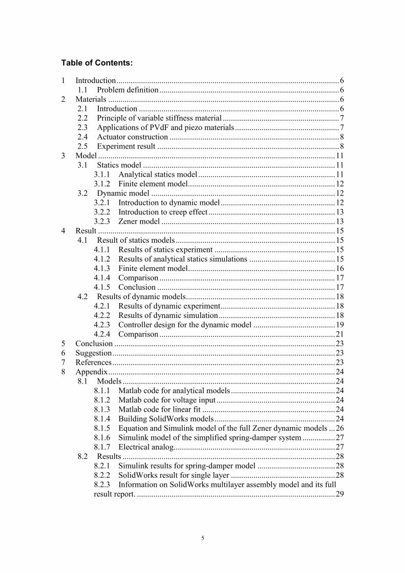
This bachelor assignment will focus on the piezo leaf spring in the VSJ. A leaf spring

with length 59.8mm, width 19.8mm and height 0.19mm is composed by a pair of

plastic covering layers, a pair of aluminum layer to provide voltage difference, an

active piezo layer and an insulating nylon layer. These springs will be put radially on

the VSJ in Figure 4. The first part of the report will focus on the material properties of

this sample.

This piezo element can change its stiffness when a voltage difference is applied. In the

second part of the report, a SolidWorks model will be built to try simulating the

bending under different stiffness (=different voltage), since the robot is designed in

SolidWorks.

Finally, the report will focus on the delay of the stiffness changes and give a physical

model describing the delay. To compensate this delay, a feedback PI controller is also

designed.

Figure 1: The geometric configurations of the leaf spring.

2 Materials

2.1 Introduction

In this chapter the principle and mechanism of the variable stiffness material are

introduced. The materials those constructing the actuator and its leaf spring are

described. An experiment about the mechanical properties is given.

7

2.2 Principle of variable stiffness material

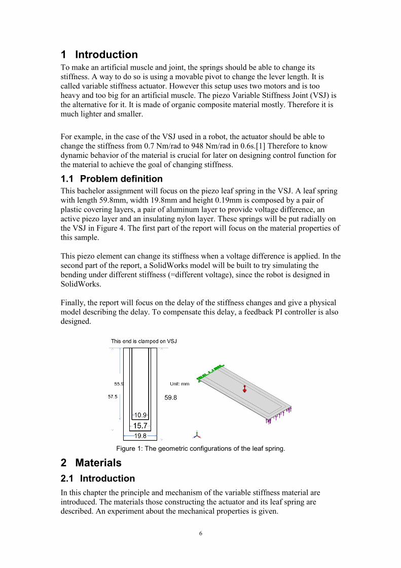
The active piezo layer of the leaf spring is mainly PVdF (polymer of copolymer of

vinylidene fluoride and trifluoroethylene (C2F2H2)n ). The theory of piezoelectric is

that electric charge is accumulated in response to stress applied on the piezo material

and reacts back to the material. In the case of the application of VSJ, by adding or

removing the charges, the mechanical behavior, the internal stress, is expected to

change.

Figure 2: The formula for PVdF

1

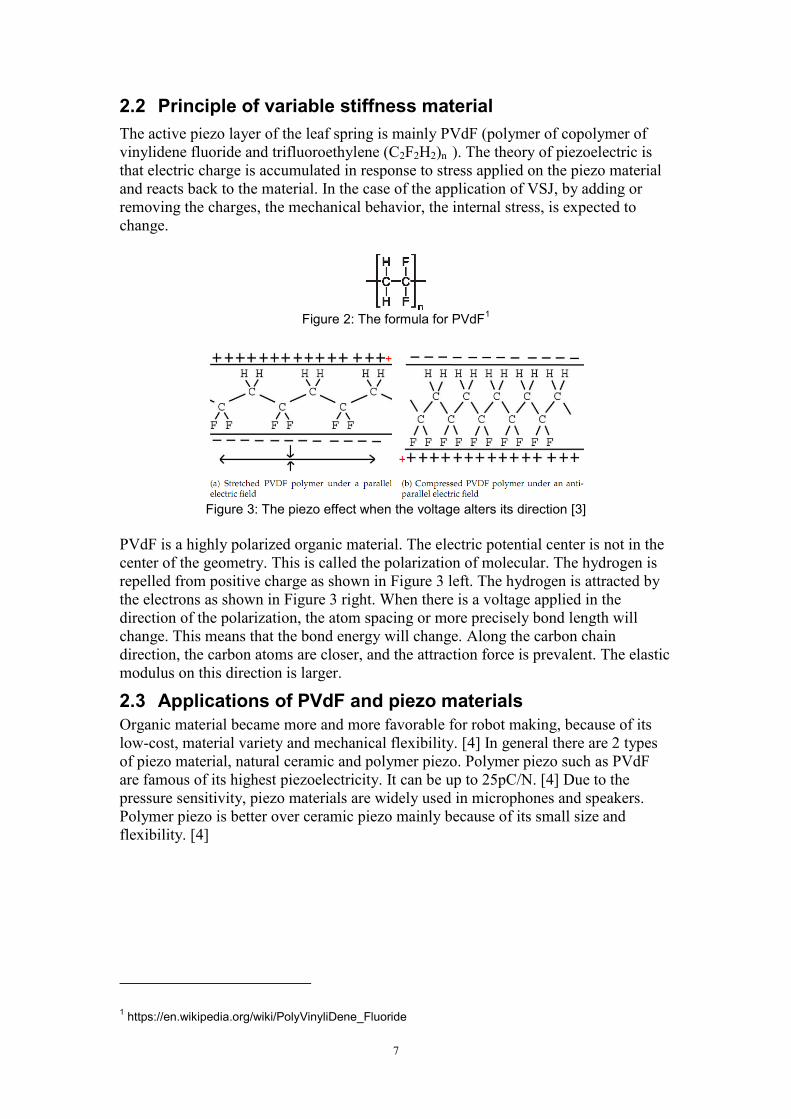
Figure 3: The piezo effect when the voltage alters its direction [3]

PVdF is a highly polarized organic material. The electric potential center is not in the

center of the geometry. This is called the polarization of molecular. The hydrogen is

repelled from positive charge as shown in Figure 3 left. The hydrogen is attracted by

the electrons as shown in Figure 3 right. When there is a voltage applied in the

direction of the polarization, the atom spacing or more precisely bond length will

change. This means that the bond energy will change. Along the carbon chain

direction, the carbon atoms are closer, and the attraction force is prevalent. The elastic

modulus on this direction is larger.

2.3 Applications of PVdF and piezo materials

Organic material became more and more favorable for robot making, because of its

low-cost, material variety and mechanical flexibility. [4] In general there are 2 types

of piezo material, natural ceramic and polymer piezo. Polymer piezo such as PVdF

are famous of its highest piezoelectricity. It can be up to 25pC/N. [4] Due to the

pressure sensitivity, piezo materials are widely used in microphones and speakers.

Polymer piezo is better over ceramic piezo mainly because of its small size and

flexibility. [4]

1 https://en.wikipedia.org/wiki/PolyVinyliDene_Fluoride

8

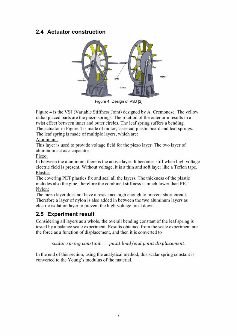
2.4 Actuator construction

Figure 4: Design of VSJ [2]

Figure 4 is the VSJ (Variable Stiffness Joint) designed by A. Cremonese. The yellow

radial placed parts are the piezo springs. The rotation of the outer arm results in a

twist effect between inner and outer circles. The leaf spring suffers a bending.

The actuator in Figure 4 is made of motor, laser-cut plastic board and leaf springs.

The leaf spring is made of multiple layers, which are:

Aluminum:

This layer is used to provide voltage field for the piezo layer. The two layer of

aluminum act as a capacitor.

Piezo:

In between the aluminum, there is the active layer. It becomes stiff when high voltage

electric field is present. Without voltage, it is a thin and soft layer like a Teflon tape.

Plastic:

The covering PET plastics fix and seal all the layers. The thickness of the plastic

includes also the glue, therefore the combined stiffness is much lower than PET.

Nylon:

The piezo layer does not have a resistance high enough to prevent short circuit.

Therefore a layer of nylon is also added in between the two aluminum layers as

electric isolation layer to prevent the high-voltage breakdown.

2.5 Experiment result

Considering all layers as a whole, the overall bending constant of the leaf spring is

tested by a balance scale experiment. Results obtained from the scale experiment are

the force as a function of displacement, and then it is converted to

.

In the end of this section, using the analytical method, this scalar spring constant is

converted to the Young‟s modulus of the material.

9

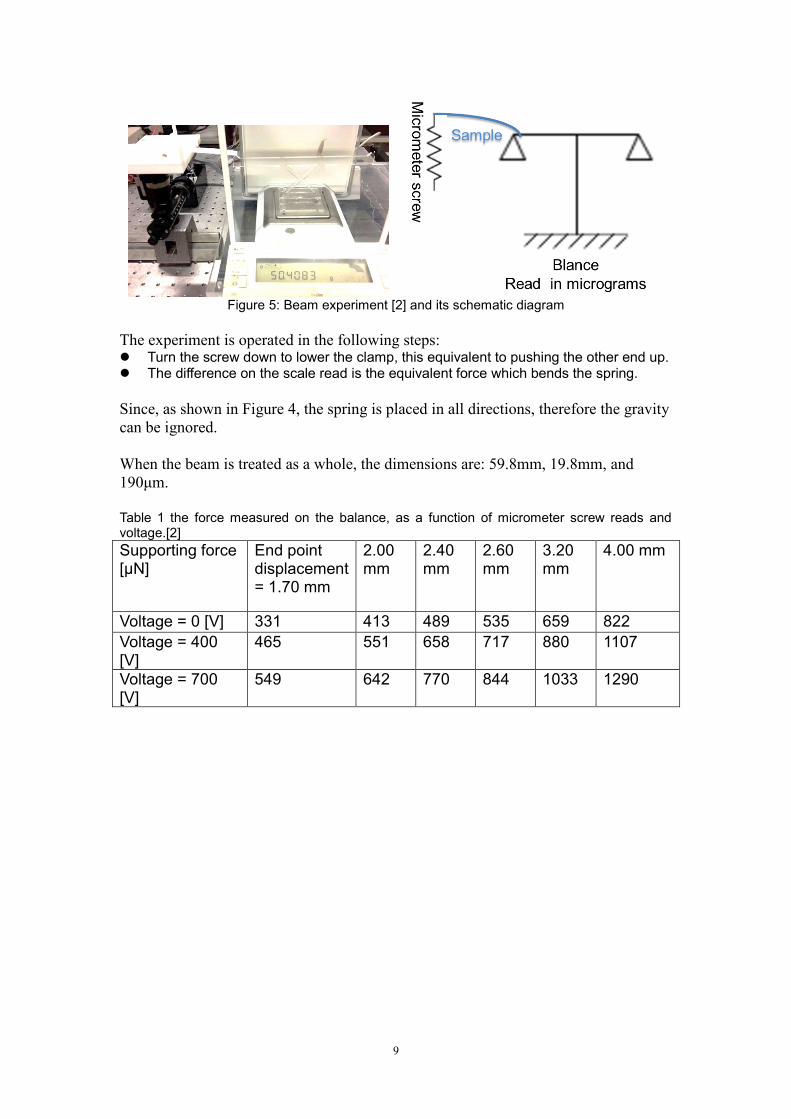
Figure 5: Beam experiment [2] and its schematic diagram

The experiment is operated in the following steps: Turn the screw down to lower the clamp, this equivalent to pushing the other end up. The difference on the scale read is the equivalent force which bends the spring.

Since, as shown in Figure 4, the spring is placed in all directions, therefore the gravity

can be ignored.

When the beam is treated as a whole, the dimensions are: 59.8mm, 19.8mm, and

190μm.

Table 1 the force measured on the balance, as a function of micrometer screw reads and voltage.[2]

Supporting force [μN]

End point displacement = 1.70 mm

2.00 mm

2.40 mm

2.60 mm

3.20 mm

4.00 mm

Voltage = 0 [V] 331 413 489 535 659 822

Voltage = 400 [V]

465 551 658 717 880 1107

Voltage = 700 [V]

549 642 770 844 1033 1290

10

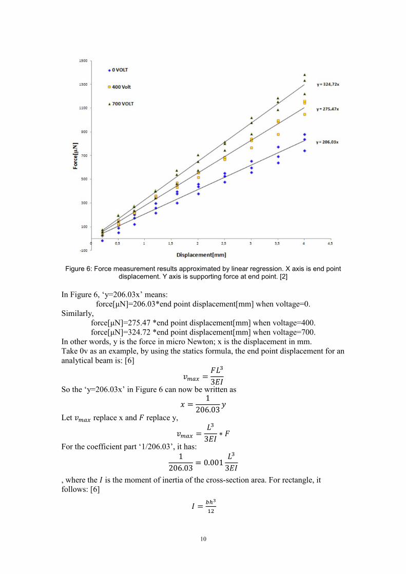
Figure 6: Force measurement results approximated by linear regression. X axis is end point

displacement. Y axis is supporting force at end point. [2]

In Figure 6, „y=206.03x‟ means:

force[μN]=206.03*end point displacement[mm] when voltage=0.

Similarly,

force[μN]=275.47 *end point displacement[mm] when voltage=400.

force[μN]=324.72 *end point displacement[mm] when voltage=700.

In other words, y is the force in micro Newton; x is the displacement in mm.

Take 0v as an example, by using the statics formula, the end point displacement for an

analytical beam is: [6]

So the „y=206.03x‟ in Figure 6 can now be written as

Let replace x and replace y,

For the coefficient part „1/206.03‟, it has:

, where the is the moment of inertia of the cross-section area. For rectangle, it

follows: [6]

11

Fill in =1.1317e-14, =59.8e-3:

, since k=206.03, 275.47, 324.72 for 0v, 400v, 700v respectively.

So, it gives E=1.298e9, 1.735e9, 2.045e9 Pa respectively.

After a linear fit using code in Appendix 8.1.3, the following voltage-stiffness relation

is found.

3 Model

3.1 Statics model

3.1.1 Analytical statics model

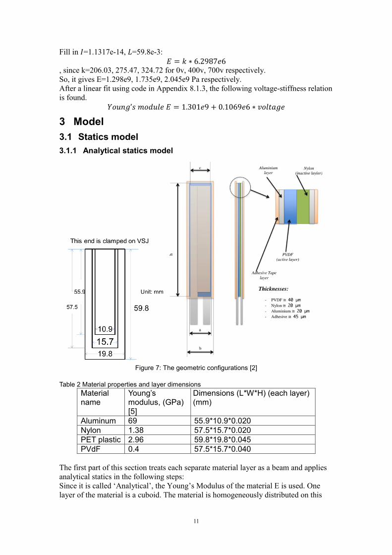
Figure 7: The geometric configurations [2]

Table 2 Material properties and layer dimensions

Material name

Young‟s modulus, (GPa) [5]

Dimensions (L*W*H) (each layer) (mm)

Aluminum 69 55.9*10.9*0.020

Nylon 1.38 57.5*15.7*0.020

PET plastic 2.96 59.8*19.8*0.045

PVdF 0.4 57.5*15.7*0.040

The first part of this section treats each separate material layer as a beam and applies

analytical statics in the following steps:

Since it is called „Analytical‟, the Young‟s Modulus of the material E is used. One

layer of the material is a cuboid. The material is homogeneously distributed on this

12

cuboid. The 3D model can be simplified to 2D model with only the longitude and the

thickness direction left. [6] Besides, the cuboid beam can be seen as a linear system.

[6] The effective external force loaded on the beam can be separated into two

components ---- the supporting force and the body weight. The supporting force in the

2D model is a point load at the end, which makes the beam curves as the following

function: [6]

( ) (1)

, where is the force, is the vertical displacement at point .

The body weight, the homogenous gravity will make the beam bend as the following

function: [6]

( ) (2)

, where is the force density along the beam length direction .

The superposition of the two is the final shape:

( )

( ) (3)

, where the is the moment of inertia of the cross-section area. For rectangle, it

follows: [6]

(4)

Thus the displacement as a function of position is described as Equation 3. The

simulation results of this model are in section 4.1.2.

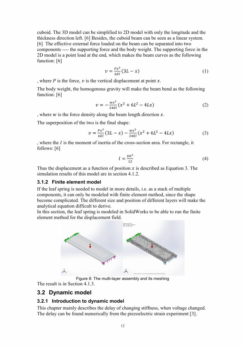
3.1.2 Finite element model

If the leaf spring is needed to model in more details, i.e. as a stack of multiple

components, it can only be modeled with finite element method, since the shape

become complicated. The different size and position of different layers will make the

analytical equation difficult to derive.

In this section, the leaf spring is modeled in SolidWorks to be able to run the finite

element method for the displacement field.

Figure 8: The multi-layer assembly and its meshing

The result is in Section 4.1.3.

3.2 Dynamic model

3.2.1 Introduction to dynamic model

This chapter mainly describes the delay of changing stiffness, when voltage changed.

The delay can be found numerically from the piezoelectric strain experiment [3].

13

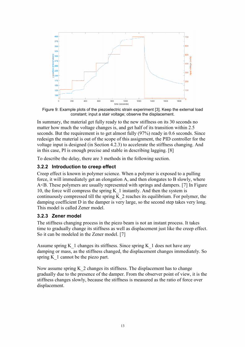
Figure 9: Example plots of the piezoelectric strain experiment [3]. Keep the external load

constant; input a stair voltage; observe the displacement.

In summary, the material get fully ready to the new stiffness on its 30 seconds no

matter how much the voltage changes is, and get half of its transition within 2.5

seconds. But the requirement is to get almost fully (97%) ready in 0.6 seconds. Since

redesign the material is out of the scope of this assignment, the PID controller for the

voltage input is designed (in Section 4.2.3) to accelerate the stiffness changing. And

in this case, PI is enough precise and stable in describing lagging. [8]

To describe the delay, there are 3 methods in the following section.

3.2.2 Introduction to creep effect

Creep effect is known in polymer science. When a polymer is exposed to a pulling

force, it will immediately get an elongation A, and then elongates to B slowly, where

A<B. These polymers are usually represented with springs and dampers. [7] In Figure

10, the force will compress the spring K_1 instantly. And then the system is

continuously compressed till the spring K_2 reaches its equilibrium. For polymer, the

damping coefficient D in the damper is very large, so the second step takes very long.

This model is called Zener model.

3.2.3 Zener model

The stiffness changing process in the piezo beam is not an instant process. It takes

time to gradually change its stiffness as well as displacement just like the creep effect.

So it can be modeled in the Zener model. [7]

Assume spring K_1 changes its stiffness. Since spring K_1 does not have any

damping or mass, as the stiffness changed, the displacement changes immediately. So

spring K_1 cannot be the piezo part.

Now assume spring K_2 changes its stiffness. The displacement has to change

gradually due to the presence of the damper. From the observer point of view, it is the

stiffness changes slowly, because the stiffness is measured as the ratio of force over

displacement.

14

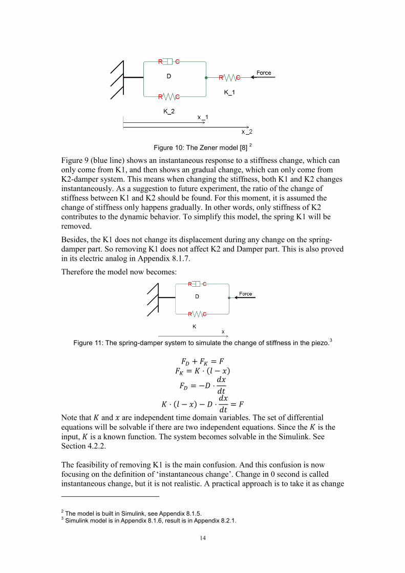
Figure 10: The Zener model [8]

2

Figure 9 (blue line) shows an instantaneous response to a stiffness change, which can

only come from K1, and then shows an gradual change, which can only come from

K2-damper system. This means when changing the stiffness, both K1 and K2 changes

instantaneously. As a suggestion to future experiment, the ratio of the change of

stiffness between K1 and K2 should be found. For this moment, it is assumed the

change of stiffness only happens gradually. In other words, only stiffness of K2

contributes to the dynamic behavior. To simplify this model, the spring K1 will be

removed.

Besides, the K1 does not change its displacement during any change on the spring-

damper part. So removing K1 does not affect K2 and Damper part. This is also proved

in its electric analog in Appendix 8.1.7.

Therefore the model now becomes:

Figure 11: The spring-damper system to simulate the change of stiffness in the piezo.

3

( )

( )

Note that and are independent time domain variables. The set of differential

equations will be solvable if there are two independent equations. Since the is the

input, is a known function. The system becomes solvable in the Simulink. See

Section 4.2.2.

The feasibility of removing K1 is the main confusion. And this confusion is now

focusing on the definition of „instantaneous change‟. Change in 0 second is called

instantaneous change, but it is not realistic. A practical approach is to take it as change

2 The model is built in Simulink, see Appendix 8.1.5.

3 Simulink model is in Appendix 8.1.6, result is in Appendix 8.2.1.

15

in a very short time, shorter than the sampling time. In the simulation results for all 3

of the Zener, Simplified-spring-damper system and the PI models (in Section 4.2.2),

they show a rapid change, which are all faster than the sample time. So they can be

taken as instantaneous change.

In Simulink for Zener model, not only the parameters but also the initial values in the

integrator are dependent on the material and assembly. The PI model (in Section

4.2.2), however, only has two parameters depend on the material and assembly. The

integrator initials are always zero, independent from the material and assembly.

So this report tries using PI model to realize the properties of Zener model. And the

steps are in Section 4.2.2. PI is just one of the many ways to (partly) describe Zener

model.

4 Result

4.1 Result of statics models

4.1.1 Results of statics experiment

The beam bending experiment has been described in section 2.5. In that section, the

bending experiment is operated on the whole sample, the obtained Young‟s modulus

is equivalent to the combination of multiple material properties.

4.1.2 Results of analytical statics simulations

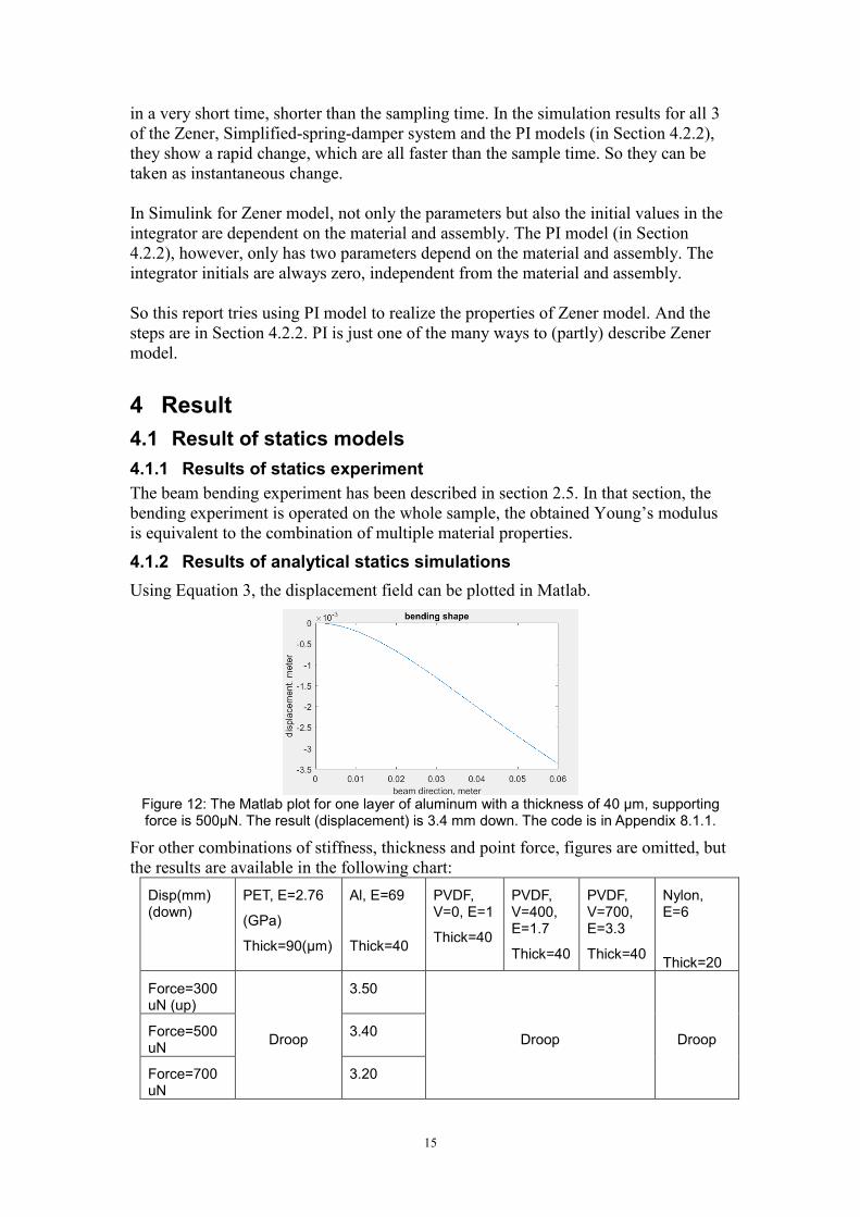
Using Equation 3, the displacement field can be plotted in Matlab.

Figure 12: The Matlab plot for one layer of aluminum with a thickness of 40 μm, supporting force is 500μN. The result (displacement) is 3.4 mm down. The code is in Appendix 8.1.1.

For other combinations of stiffness, thickness and point force, figures are omitted, but

the results are available in the following chart:

Disp(mm) (down)

PET, E=2.76

(GPa)

Thick=90(μm)

Al, E=69

Thick=40

PVDF, V=0, E=1

Thick=40

PVDF, V=400, E=1.7

Thick=40

PVDF, V=700, E=3.3

Thick=40

Nylon, E=6

Thick=20

Force=300 uN (up)

Droop

3.50

Droop Droop Force=500 uN

3.40

Force=700 uN

3.20

16

Force=900 uN

3.00

In the table above, droop means the material is too soft and it completely bends down.

In other words, it is out of the linear deformation range. Therefore in the per layer

analysis, only the results for the aluminum layer is useful.

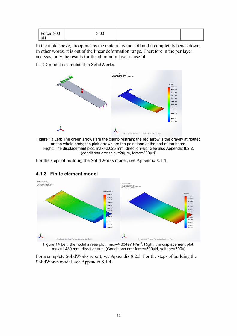
Its 3D model is simulated in SolidWorks.

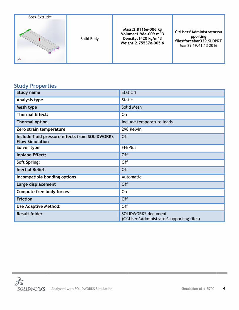
Figure 13 Left: The green arrows are the clamp restrain; the red arrow is the gravity attributed

on the whole body; the pink arrows are the point load at the end of the beam. Right: The displacement plot, max=2.025 mm, direction=up. See also Appendix 8.2.2.

(conditions are: thick=20μm, force=300μN)

For the steps of building the SolidWorks model, see Appendix 8.1.4.

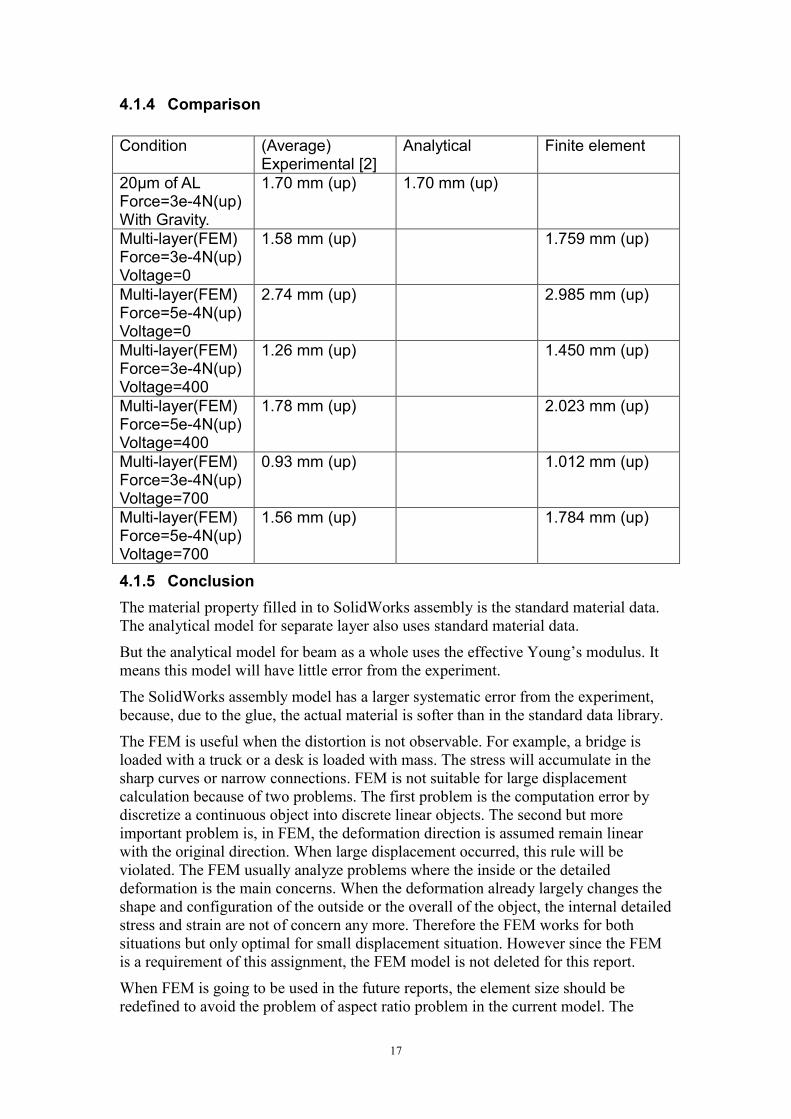
4.1.3 Finite element model

Figure 14 Left: the nodal stress plot, max=4.334e7 N/m

2. Right: the displacement plot,

max=1.439 mm, direction=up. (Conditions are: force=500μN, voltage=700v)

For a complete SolidWorks report, see Appendix 8.2.3. For the steps of building the

SolidWorks model, see Appendix 8.1.4.

17

4.1.4 Comparison

Condition (Average) Experimental [2]

Analytical Finite element

20μm of AL Force=3e-4N(up) With Gravity.

1.70 mm (up) 1.70 mm (up)

Multi-layer(FEM) Force=3e-4N(up) Voltage=0

1.58 mm (up) 1.759 mm (up)


2.74 mm (up) 2.985 mm (up)


1.26 mm (up) 1.450 mm (up)


1.78 mm (up) 2.023 mm (up)


0.93 mm (up) 1.012 mm (up)


1.56 mm (up) 1.784 mm (up)

4.1.5 Conclusion

The material property filled in to SolidWorks assembly is the standard material data.

The analytical model for separate layer also uses standard material data.

But the analytical model for beam as a whole uses the effective Young‟s modulus. It

means this model will have little error from the experiment.

The SolidWorks assembly model has a larger systematic error from the experiment,

because, due to the glue, the actual material is softer than in the standard data library.

The FEM is useful when the distortion is not observable. For example, a bridge is

loaded with a truck or a desk is loaded with mass. The stress will accumulate in the

sharp curves or narrow connections. FEM is not suitable for large displacement

calculation because of two problems. The first problem is the computation error by

discretize a continuous object into discrete linear objects. The second but more

important problem is, in FEM, the deformation direction is assumed remain linear

with the original direction. When large displacement occurred, this rule will be

violated. The FEM usually analyze problems where the inside or the detailed

deformation is the main concerns. When the deformation already largely changes the

shape and configuration of the outside or the overall of the object, the internal detailed

stress and strain are not of concern any more. Therefore the FEM works for both

situations but only optimal for small displacement situation. However since the FEM

is a requirement of this assignment, the FEM model is not deleted for this report.

When FEM is going to be used in the future reports, the element size should be

redefined to avoid the problem of aspect ratio problem in the current model. The

18

average ratio of length, width and height of the 3D element after meshing is called

aspect ratio. In the per layer simulation, the aspect ratio is about 110. In the multi-

layer simulation, the aspect ratio is about 700. In Finite Element Theory, an

acceptable aspect ratio has to be less than 3. The per-layer model and the multi-layer

model have aspect ratio out of this range, the calculating error is uncontrollable. This

is because, for this sample, length:height=3000:1 approximately. However if the

optimal aspect ratio 1.5 is chosen, about 10 million elements will be created. This is

out of the range of the memory of a personal computer.

The whole-beam model, which treats all layers as a whole, has an aspect ratio about

10, which makes the error in a reasonable range comparing to the other two models.

In addition to the aspect ratio, there is a problem about the vague definition of gluing

the sample. In the SolidWorks model, parts are connected with locking. In practice,

for the available samples, the connection may not be very good. But measuring the

sliding coefficient is of no use, since these samples are made by hand and may vary a

lot.

4.2 Results of dynamic models

4.2.1 Results of dynamic experiment

The test of impulse response and frequency response of the sample is mainly

described in section 3.2.1.

4.2.2 Results of dynamic simulation

The creep analog and the electrical analog use differential equation model. It is

sensitive to the initial condition and the parameters. Therefore the model is not easy to

adapt the parameter changes. The previous report by Visschers had given the impulse

response by voltage-strain measurements. On a modeling and controller designing

propose, this impulse response model will be enough. It is

, where are constants. [3]

It is a solution to the first order differential equation given in Section 3.2.3.

And the time constant is found to be 5s for -3dB and 30s for settle point. Using this

system transfer function, it is found by trial that the following equations have such

impulse response as well:

( )

(5)

( ) ( ) ∫ ( )

(6)

, where ( ) is the system output, ( ) is the error on the feedback loop.

A proportion and integration feedback loop can describe equation (5) and (6). In

Figure 15, the plant contains the PI feedback loop. The piezo plant first compute the

normalized stiffness and output to port2 for observation, and then compute the

stiffness.

19

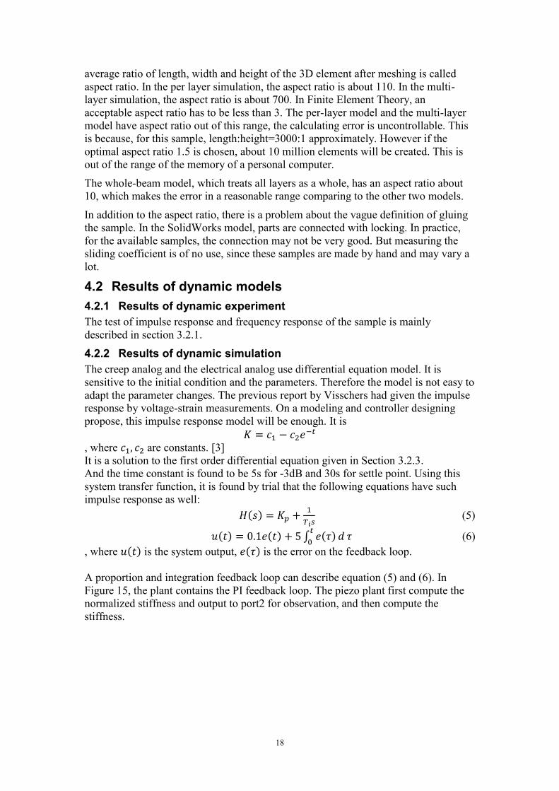
Figure 15: The exploded view of the group „plant‟ in the Simulink model.

Increasing the gain will make the system react faster, but will also introduce

overshoot. The gain Ki 0.1 and gain Ti 0.2 are found by trial. They can make the

reaction curve accurate enough to describe the material dynamic.

For control propose, the out1 is the stiffness, meanwhile the out2 is the normalized

stiffness which follows the equation below.

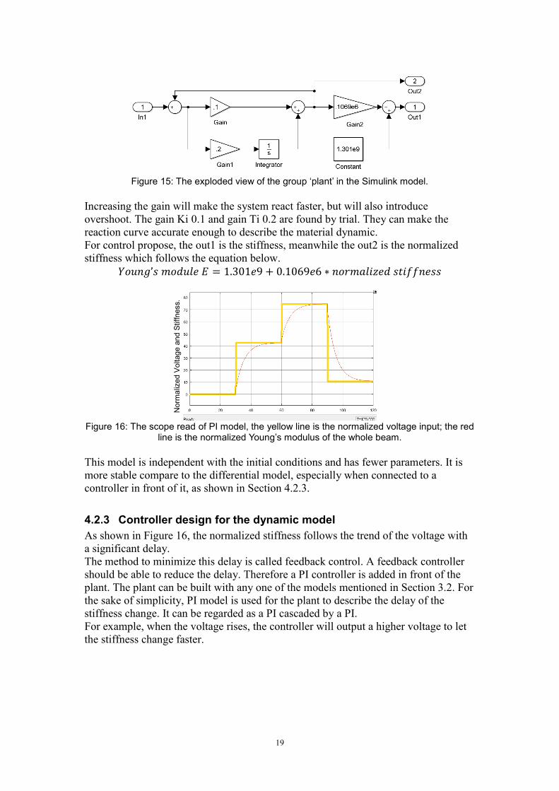
Figure 16: The scope read of PI model, the yellow line is the normalized voltage input; the red

line is the normalized Young‟s modulus of the whole beam.

This model is independent with the initial conditions and has fewer parameters. It is

more stable compare to the differential model, especially when connected to a

controller in front of it, as shown in Section 4.2.3.

4.2.3 Controller design for the dynamic model

As shown in Figure 16, the normalized stiffness follows the trend of the voltage with

a significant delay.

The method to minimize this delay is called feedback control. A feedback controller

should be able to reduce the delay. Therefore a PI controller is added in front of the

plant. The plant can be built with any one of the models mentioned in Section 3.2. For

the sake of simplicity, PI model is used for the plant to describe the delay of the

stiffness change. It can be regarded as a PI cascaded by a PI.

For example, when the voltage rises, the controller will output a higher voltage to let

the stiffness change faster.

Norm

aliz

ed V

oltage a

nd S

tiff

ness.

20

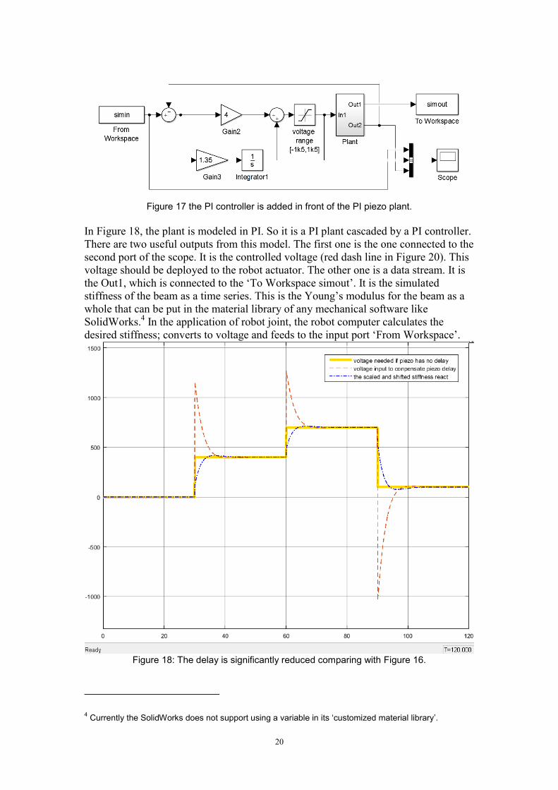
Figure 17 the PI controller is added in front of the PI piezo plant.

In Figure 18, the plant is modeled in PI. So it is a PI plant cascaded by a PI controller.

There are two useful outputs from this model. The first one is the one connected to the

second port of the scope. It is the controlled voltage (red dash line in Figure 20). This

voltage should be deployed to the robot actuator. The other one is a data stream. It is

the Out1, which is connected to the „To Workspace simout‟. It is the simulated

stiffness of the beam as a time series. This is the Young‟s modulus for the beam as a

whole that can be put in the material library of any mechanical software like

SolidWorks.4 In the application of robot joint, the robot computer calculates the

desired stiffness; converts to voltage and feeds to the input port „From Workspace‟.

Figure 18: The delay is significantly reduced comparing with Figure 16.

4 Currently the SolidWorks does not support using a variable in its „customized material library‟.

21

The third method finally outputs the elasticity Young‟s modulus that can be read by

other simulation software. For example use a variable in the Elastic Modulus of the

customized material.

4.2.4 Comparison

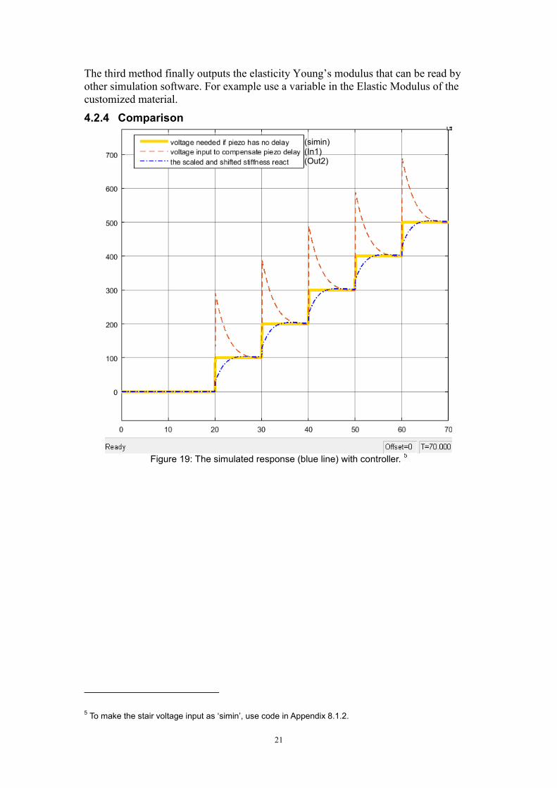
Figure 19: The simulated response (blue line) with controller.

5

5 To make the stair voltage input as „simin‟, use code in Appendix 8.1.2.

(simin) (In1) (Out2)

22

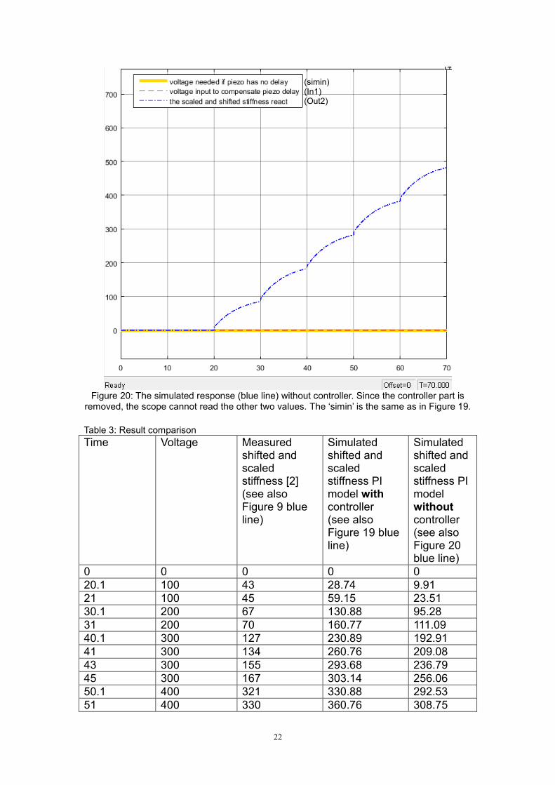
Figure 20: The simulated response (blue line) without controller. Since the controller part is

removed, the scope cannot read the other two values. The „simin‟ is the same as in Figure 19.

Table 3: Result comparison

Time Voltage Measured shifted and scaled stiffness [2] (see also Figure 9 blue line)

Simulated shifted and scaled stiffness PI model with controller (see also Figure 19 blue line)

Simulated shifted and scaled stiffness PI model without controller (see also Figure 20 blue line)

0 0 0 0 0

20.1 100 43 28.74 9.91

21 100 45 59.15 23.51

30.1 200 67 130.88 95.28

31 200 70 160.77 111.09

40.1 300 127 230.89 192.91

41 300 134 260.76 209.08

43 300 155 293.68 236.79

45 300 167 303.14 256.06

50.1 400 321 330.88 292.53

51 400 330 360.76 308.75

(simin) (In1) (Out2)

23

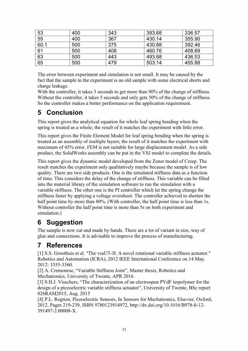
53 400 343 393.68 336.57

55 400 367 430.14 355.90

60.1 500 375 430.88 392.46

61 500 408 460.76 408.69

63 500 443 493.68 436.53

65 500 479 503.14 455.88

The error between experiment and simulation is not small. It may be caused by the

fact that the sample in the experiment is an old sample with some electrical shorts and

charge leakage.

With the controller, it takes 3 seconds to get more than 90% of the change of stiffness.

Without the controller, it takes 5 seconds and only gets 50% of the change of stiffness.

So the controller makes a better performance on the application requirement.

5 Conclusion

This report gives the analytical equation for whole leaf spring bending when the

spring is treated as a whole; the result of it matches the experiment with little error.

This report gives the Finite Element Model for leaf spring bending when the spring is

treated as an assembly of multiple layers; the result of it matches the experiment with

maximum of 45% error. FEM is not suitable for large displacement model. As a side

product, the SolidWorks assembly can be put in the VSJ model to complete the details.

This report gives the dynamic model developed from the Zener model of Creep. The

result matches the experiment only qualitatively maybe because the sample is of low

quality. There are two side products. One is the simulated stiffness data as a function

of time. This considers the delay of the change of stiffness. This variable can be filled

into the material library of the simulation software to run the simulation with a

variable stiffness. The other one is the PI controller which let the spring change the

stiffness faster by applying a voltage overshoot. The controller achieved to shorten the

half point time by more than 80%. (With controller, the half point time is less than 1s.

Without controller the half point time is more than 5s on both experiment and

simulation.)

6 Suggestion The sample is now cut and made by hands. There are a lot of variant in size, way of

glue and connections. It is advisable to improve the process of manufacturing.

7 References [1] S.S. Groothuis et al. "The vsaUT-II: A novel rotational variable stiffness actuator."

Robotics and Automation (ICRA), 2012 IEEE International Conference on 14 May.

2012: 3355-3360.

[2] A. Cremonese, “Variable Stiffness Joint”, Master thesis, Robotics and

Mechatronics, University of Twente, APR 2016.

[3] S.H.J. Visschers, “The characterization of an electrospun PVdF terpolymer for the

design of a piezoelectric variable stiffness actuator”, University of Twente, BSc report

026RAM2015, Aug. 2015

[4] P.L. Regtien, Piezoelectric Sensors, In Sensors for Mechatronics, Elsevier, Oxford,

2012, Pages 219-239, ISBN 9780123914972, http://dx.doi.org/10.1016/B978-0-12-

391497-2.00008-X.

http://dx.doi.org/10.1016/B978-0-12-391497-2.00008-X

http://dx.doi.org/10.1016/B978-0-12-391497-2.00008-X

24

[5] W.D. Callister and D.G. Rethwisch, Fundamentals of Materials Science and

Engineering, 4th edition, John Wiley & Sons, 2012, ISBN 9781118061602.

[6] R.C. Hibbeler, Statics and Mechanics of Material, 12th

edition, Pearson Education,

2011, ISBN 9789810686321.

[7] N.G. McCrum, Principles of Polymer Engineering, 2nd

edition, Oxford University

Press, 1997, ISBN 9780198565260.

[8] H. Meng, The Principle of Automatic Control, 2nd

edition, China Machine Press,

2013, ISBN 9787111448273.

8 Appendix

8.1 Models

8.1.1 Matlab code for analytical models E=69e9;%material

L=59.8e-3;

P=900e-6;%force

x=1e-3*59.8;%for multiple point, say x=1e-3*[.1:.1:59.8];

%for end-point only, say x=1e-3*59.8

b=19.8e-3;

h=20e-6;%thick

I=(b*h^3)/12;

mcl=2700*1*b*h;%density e.g. 2.7g/cm3, fill in mcl=2700*1*b*h= how many kg a

1 meter long such beam

w=mcl*9.8/1;

v=(x.^2*P)/(6*E*I).*(3*L-x)-(w*x.^2)/(24*E*I).*(x.^2+6*L^2-4*L*x) %positive

direction up, so gravity down

8.1.2 Matlab code for voltage input t=[.1:.1:70];

v(1:200)=0;

v(201:300)=100;

v(301:400)=200;

v(401:500)=300;

v(501:600)=400;

v(601:700)=500;

simin=[t;v]';

8.1.3 Matlab code for linear fit >> st=1e9*[1.298,1.735,2.045]';vt=1e2*[0,4,7]';

>> f0=fit(vt,st,'poly1')

f0 = Linear model Poly1:

f0(x) = p1*x + p2

Coefficients (with 95% confidence bounds):

p1 = 1.069e+06 (8.574e+05, 1.28e+06)

p2 = 1.301e+09 (1.203e+09, 1.399e+09)

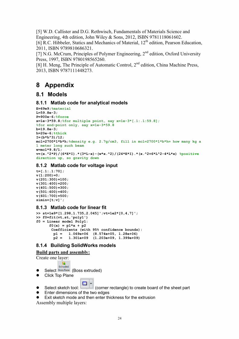
8.1.4 Building SolidWorks models

Build parts and assembly:

Create one layer:

Select (Boss extruded) Click Top Plane

Select sketch tool: (corner rectangle) to create board of the sheet part Enter dimensions of the two edges Exit sketch mode and then enter thickness for the extrusion

Assembly multiple layers:

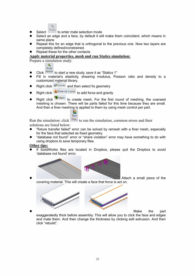
25

Select to enter mate selection mode Select an edge and a face, by default it will make them coincident, which means in

same plane Repeat this for an edge that is orthogonal to the previous one. Now two layers are

completely defined/constrained. Repeat these for the other contacts

Apply material properties, mesh and run Statics simulation:

Prepare a simulation study:

Click to start a new study, save it as “Statics 1” Fill in material‟s elasticity, shearing modulus, Poisson ratio and density to a

customized material library.

Right click and then select fix geometry

Right click to add force and gravity

Right click to create mesh, For the first round of meshing, the coarsest meshing is chosen. There will be parts failed for this time because they are small. And then a finer meshing is applied to them by using mesh control per part.

Run the simulation: click to run the simulation, common errors and their

solutions are listed below: "fixture transfer failed" error can be solved by remesh with a finer mesh, especially

for the face that selected as fixed geometry. “database not found‟‟ error or “share violation” error may have something to do with

using dropbox to save temporary files.

Other tips: If SolidWorks files are located in Dropbox, please quit the Dropbox to avoid

„database not found‟ error.

Attach a small piece of the covering material. This will create a face that force is act on.

Make the part exaggeratedly thick before assembly. This will allow you to click the face and edges and mate them. And then change the thickness by clicking edit extrusion. And then click “rebuild”.

26

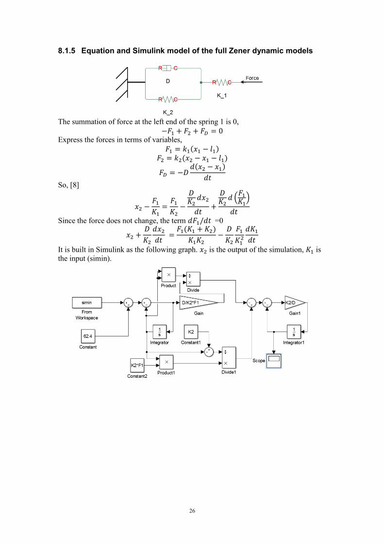
8.1.5 Equation and Simulink model of the full Zener dynamic models

The summation of force at the left end of the spring 1 is 0,

Express the forces in terms of variables,

( ) ( )

( )

So, [8]

( )

Since the force does not change, the term =0

( )

It is built in Simulink as the following graph. is the output of the simulation, is

the input (simin).

27

8.1.6 Simulink model of the simplified spring-damper system

Result of it is in Appendix 8.2.1

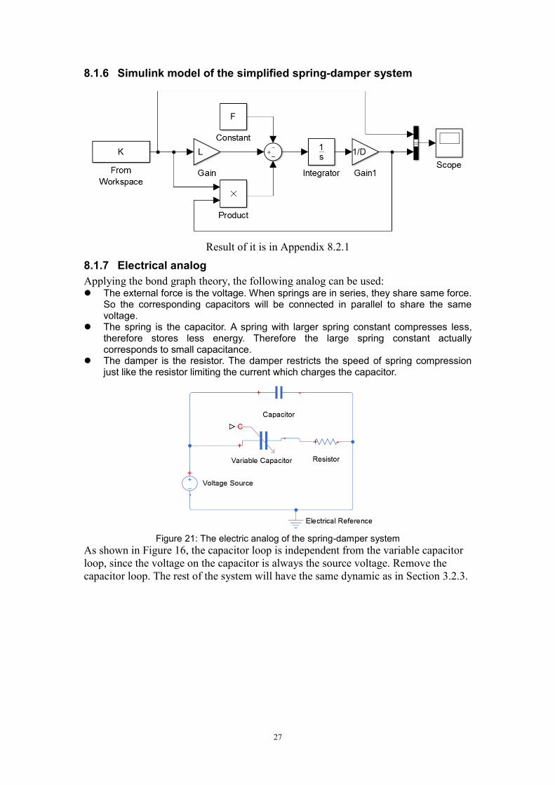
8.1.7 Electrical analog

Applying the bond graph theory, the following analog can be used: The external force is the voltage. When springs are in series, they share same force.

So the corresponding capacitors will be connected in parallel to share the same voltage.

The spring is the capacitor. A spring with larger spring constant compresses less, therefore stores less energy. Therefore the large spring constant actually corresponds to small capacitance.

The damper is the resistor. The damper restricts the speed of spring compression just like the resistor limiting the current which charges the capacitor.

Figure 21: The electric analog of the spring-damper system

As shown in Figure 16, the capacitor loop is independent from the variable capacitor

loop, since the voltage on the capacitor is always the source voltage. Remove the

capacitor loop. The rest of the system will have the same dynamic as in Section 3.2.3.

28

8.2 Results

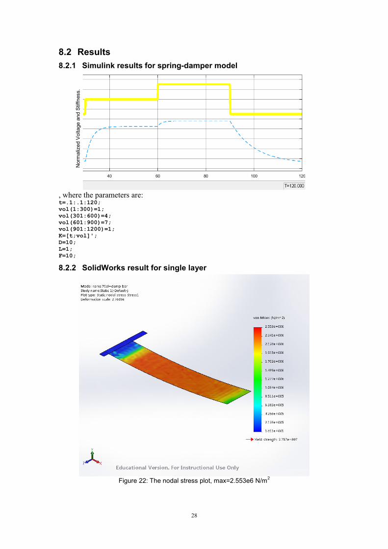
8.2.1 Simulink results for spring-damper model

, where the parameters are: t=.1:.1:120;

vol(1:300)=1;

vol(301:600)=4;

vol(601:900)=7;

vol(901:1200)=1;

K=[t;vol]';

D=10;

L=1;

F=10;

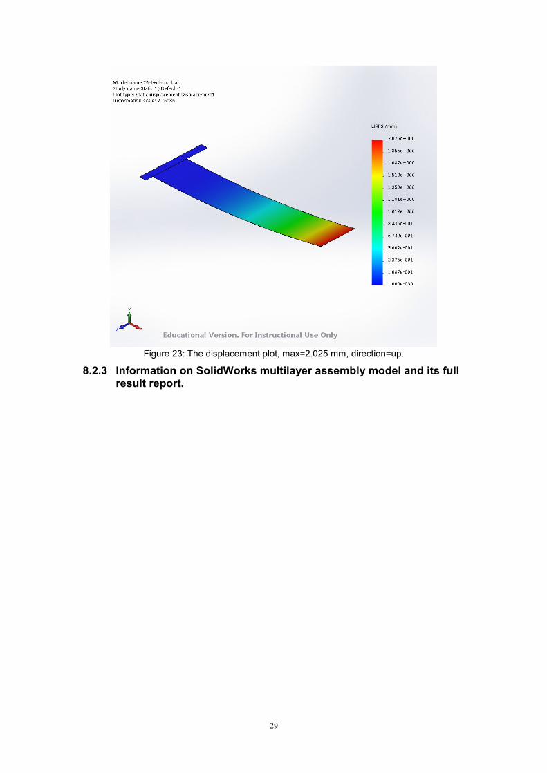
8.2.2 SolidWorks result for single layer

Figure 22: The nodal stress plot, max=2.553e6 N/m

2

Norm

aliz

ed V

oltage a

nd S

tiff

ness.

29

Figure 23: The displacement plot, max=2.025 mm, direction=up.

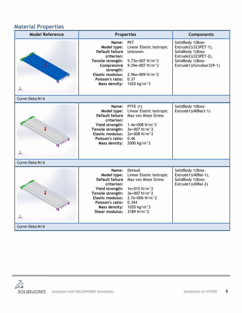
8.2.3 Information on SolidWorks multilayer assembly model and its full result report.

Analyzed with SOLIDWORKS Simulation Simulation of 415700 2

Model Information

Model name: 415700

Current Configuration: Default

Solid Bodies

Document Name and Reference

Treated As Volumetric Properties Document Path/Date

Modified

Boss-Extrude2

Solid Body

Mass:7.56602e-005 kg Volume:5.32818e-008 m^3

Density:1420 kg/m^3 Weight:0.00074147 N

C:\Users\Administrator\supporting

files\323PET.SLDPRT Apr 10 18:52:11 2016


Boss-Extrude2

Solid Body




files\323PET.SLDPRT Apr 10 18:52:11 2016

Boss-Extrude1

Solid Body




files\408act.SLDPRT Apr 08 13:13:27 2016

Boss-Extrude1

Solid Body




files\408al.SLDPRT Apr 10 18:52:11 2016

Boss-Extrude1

Solid Body




files\408al.SLDPRT Apr 10 18:52:11 2016

Boss-Extrude1

Solid Body




files\408nyl.SLDPRT Apr 08 13:13:27 2016


Boss-Extrude1

Solid Body

Mass:2.8116e-006 kg Volume:1.98e-009 m^3 Density:1420 kg/m^3

Weight:2.75537e-005 N


files\forcebar329.SLDPRT Mar 29 19:41:13 2016

Study Properties Study name Static 1

Analysis type Static

Mesh type Solid Mesh

Thermal Effect: On

Thermal option Include temperature loads

Zero strain temperature 298 Kelvin

Include fluid pressure effects from SOLIDWORKS Flow Simulation

Off

Solver type FFEPlus

Inplane Effect: Off

Soft Spring: Off

Inertial Relief: Off

Incompatible bonding options Automatic

Large displacement Off

Compute free body forces On

Friction Off

Use Adaptive Method: Off

Result folder SOLIDWORKS document (C:\Users\Administrator\supporting files)


Units Unit system: SI (MKS)

Length/Displacement mm

Temperature Kelvin

Angular velocity Rad/sec

Pressure/Stress N/m^2


Material Properties

Model Reference Properties Components

Name: PET Model type: Linear Elastic Isotropic

Default failure criterion:

Unknown

Tensile strength: 5.73e+007 N/m^2 Compressive

strength: 9.29e+007 N/m^2

Elastic modulus: 2.96e+009 N/m^2 Poisson's ratio: 0.37

Mass density: 1420 kg/m^3

SolidBody 1(Boss-Extrude2)(323PET-1), SolidBody 1(Boss-Extrude2)(323PET-2), SolidBody 1(Boss-Extrude1)(forcebar329-1)

Curve Data:N/A

Name: PTFE (1) Model type: Linear Elastic Isotropic


Max von Mises Stress

Yield strength: 1.4e+008 N/m^2 Tensile strength: 3e+007 N/m^2 Elastic modulus: 2e+008 N/m^2

Poisson's ratio: 0.46 Mass density: 2000 kg/m^3

SolidBody 1(Boss-Extrude1)(408act-1)

Curve Data:N/A

Name: Default Model type: Linear Elastic Isotropic



Yield strength: 1e+015 N/m^2 Tensile strength: 3e+007 N/m^2 Elastic modulus: 2.7e+006 N/m^2


Shear modulus: 3189 N/m^2

SolidBody 1(Boss-Extrude1)(408al-1), SolidBody 1(Boss-Extrude1)(408al-2)

Curve Data:N/A


Name: Nylon 101 Model type: Linear Elastic Isotropic



Yield strength: 6e+007 N/m^2 Tensile strength: 7.92897e+007 N/m^2 Elastic modulus: 1e+009 N/m^2


Thermal expansion coefficient:

1e-006 /Kelvin

SolidBody 1(Boss-Extrude1)(408nyl-1)

Curve Data:N/A


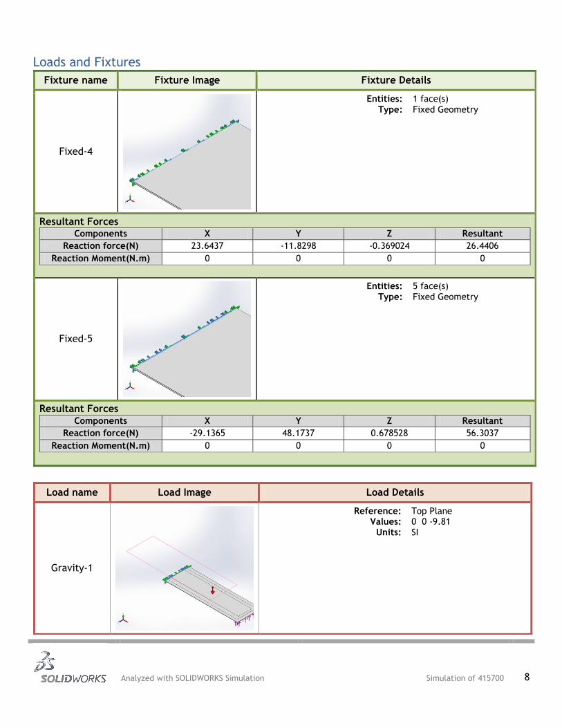
Loads and Fixtures

Fixture name Fixture Image Fixture Details

Fixed-4

Entities: 1 face(s) Type: Fixed Geometry

Resultant Forces Components X Y Z Resultant

Reaction force(N) 23.6437 -11.8298 -0.369024 26.4406

Reaction Moment(N.m) 0 0 0 0

Fixed-5

Entities: 5 face(s) Type: Fixed Geometry

Resultant Forces Components X Y Z Resultant

Reaction force(N) -29.1365 48.1737 0.678528 56.3037

Reaction Moment(N.m) 0 0 0 0

Load name Load Image Load Details

Gravity-1

Reference: Top Plane Values: 0 0 -9.81

Units: SI


Force-1

Entities: 1 face(s) Type: Apply normal force

Value: 0.15 N

Connector Definitions No Data


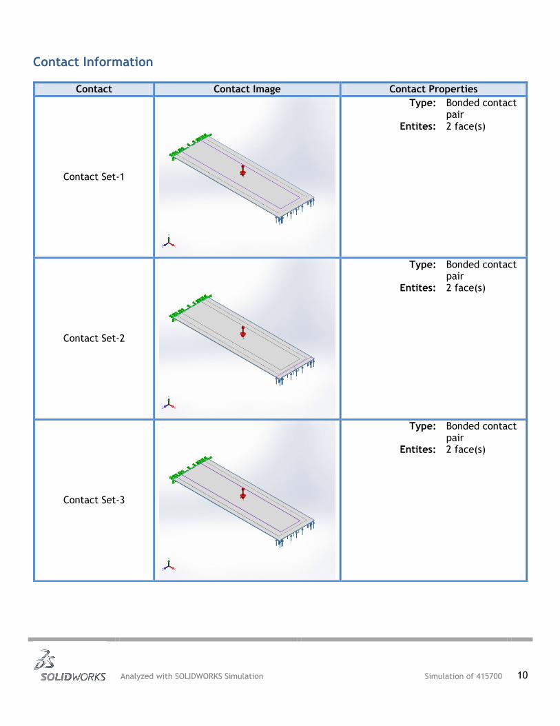
Contact Information

Contact Contact Image Contact Properties

Contact Set-1

Type: Bonded contact pair

Entites: 2 face(s)

Contact Set-2


Entites: 2 face(s)

Contact Set-3


Entites: 2 face(s)


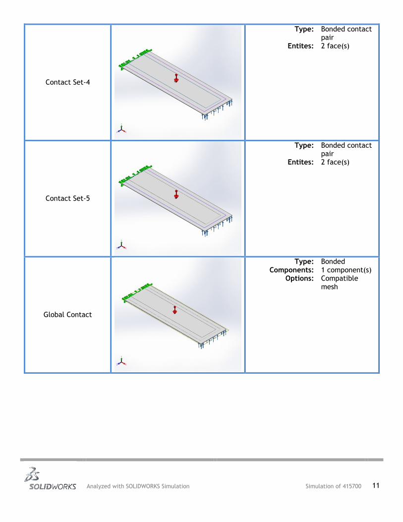
Contact Set-4


Entites: 2 face(s)

Contact Set-5


Entites: 2 face(s)

Global Contact

Type: Bonded Components: 1 component(s)

Options: Compatible mesh


Mesh information Mesh type Solid Mesh

Mesher Used: Curvature based mesh

Jacobian points 4 Points

Maximum element size 2.08751 mm

Minimum element size 2.08751 mm

Mesh Quality High

Remesh failed parts with incompatible mesh Off

Mesh information - Details

Total Nodes 20500

Total Elements 11257

Maximum Aspect Ratio 7682.2

% of elements with Aspect Ratio < 3 0

% of elements with Aspect Ratio > 10 100

% of distorted elements(Jacobian) 0

Time to complete mesh(hh;mm;ss): 00:00:04

Computer name: WIN7X200S


Mesh Control Information:

Mesh Control Name Mesh Control Image Mesh Control Details

Control-1

Entities: 5 Solid Body (s) Units: mm Size: 1.93095

Ratio: 1.5


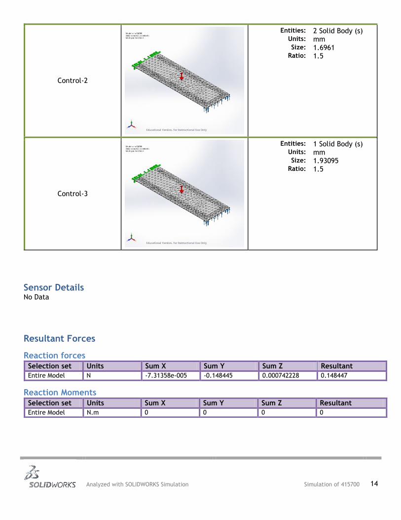
Control-2


Ratio: 1.5

Control-3


Ratio: 1.5

Sensor Details No Data

Resultant Forces

Reaction forces

Selection set Units Sum X Sum Y Sum Z Resultant

Entire Model N -7.31358e-005 -0.148445 0.000742228 0.148447

Reaction Moments

Selection set Units Sum X Sum Y Sum Z Resultant

Entire Model N.m 0 0 0 0


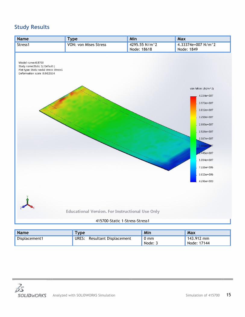
Study Results

Name Type Min Max

Stress1 VON: von Mises Stress 4295.55 N/m^2 Node: 18618

4.33374e+007 N/m^2 Node: 1849

415700-Static 1-Stress-Stress1

Name Type Min Max

Displacement1 URES: Resultant Displacement 0 mm Node: 3

143.912 mm Node: 17144


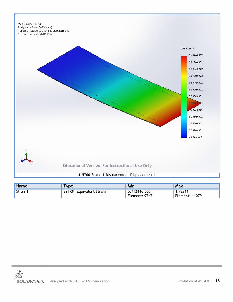
415700-Static 1-Displacement-Displacement1

Name Type Min Max

Strain1 ESTRN: Equivalent Strain 5.71244e-005 Element: 9747

1.72311 Element: 11079

Documents

Modeling of a Piezoelectric Beam Spring X. (Xinran) Liu BSc