Embed Size (px)
Citation preview
General rights Copyright and moral rights for the publications made accessible in the public portal are retained by the authors and/or other copyright owners and it is a condition of accessing publications that users recognise and abide by the legal requirements associated with these rights.
Users may download and print one copy of any publication from the public portal for the purpose of private study or research.
You may not further distribute the material or use it for any profit-making activity or commercial gain
You may freely distribute the URL identifying the publication in the public portal If you believe that this document breaches copyright please contact us providing details, and we will remove access to the work immediately and investigate your claim.
Downloaded from orbit.dtu.dk on: Jul 14, 2022
Microwave Activation ofDrug Release.
Jónasson, Sævar Þór
Publication date:2014
Document VersionPublisher's PDF, also known as Version of record
Link back to DTU Orbit
Citation (APA):Jónasson, S. Þ. (2014). Microwave Activation of Drug Release. DTU Elektro.
Sævar Þór Jónasson
Microwave Activation of Drug Release PhD thesis, September 2014

The work presented in this thesis was carried out at the Departmentof Electrical Engineering in partial fulfillment of the requirements for
the PhD degree at the Technical University of Denmark.
Supervisors:
Tom Keinicke Johansen, Associate Professor, PhD,Vitaliy Zhurbenko, Assistant Professor, PhD,Department of Electrical Engineering,Technical University of Denmark
www.elektro.dtu.dk
i
Preface
This thesis is submitted as a part of the requirements to achieve the PhDdegree at the Department of Electrical Engineering, Technical Universityof Danmark. The PhD study was carried out from November 1st, 2009 toMarch 31st, 2013, with the exception of September 14th 2012 to Novem-ber 26th 2012. From January 1st 2011 to June 30st 2011 I had an ex-ternal research stay at the Department of Biomedical Engineering, Reyk-javik University under the supervision of Prof. Ceon Ramon. Financialsupport for the PhD Study was provided by the Villum Kann RasmussenFonden as a part of the NAMEC (NAno MEChanical sensors and actu-ator, http://www.namec.dtu.dk/) consortium, consisting of members fromDTU-Elektro, DTU-Nanotech, DTU-Mathematics and KU-Pharma. Asso-ciate Professor Tom Keinicke Johansen acted as the main project supervisorand Assistant Professor Vitaliy Zhurbenko as the co-supervisor.
ii
Acknowledgements
I would like to begin by thanking my former supervisor, Prof. Viktor Krozerfor encouraging me and giving me the opportunity of persuing a PhD atthe Technical University of Denmark within a field of my special interest.Secondly, I would like to thank my supervisors Associate Prof. Tom KeinickeJohansen and Assistant Prof. Vitaliy Zhurbenko for being there when Ineeded it. PhD students Brian Sveistrup Jensen and Carlos Cilla Hernandezshould receive special gratitude for our many scientific and non-scientificdiscussions.
I would like to thank DTU Elektro’s mechanical workshop for all theirassistance on the mechanical parts and technician Bo Brændstrup for hissupport. I express my gratitude to Associate Prof. Sergey Pivnenko forall his antenna measurements for me and researcher Tonny Rubæk for hisassistance in COMSOL and LabView. Associate Prof. Samel Arslanagic alsodeserves thanks for his assistance. Special thanks goes out to Prof. CeonRamon and Associate Prof. Haraldur Auðunsson for their hospitality duringmy external stay.
I thank my whole family, my parents Jónas and Edda, my sister Erlaand my brother Arnór for understanding my situation and my limited timeduring this work.
This work is in its entirety dedicated to my son Isaac Jónas Sævarssonwho is always in my heart and on my mind.
Technical University of DenmarkKgs. Lyngby, Denmark
September, 2014
Sævar Þór Jónasson
iii
Abstract
Due to current limitations in control of pharmaceutical drug release in thebody along with increasing medicine use, methods of externally-controlleddrug release are of high interest. In this thesis, the use of microwaves isproposed as a technique with the purpose of externally activating pharma-ceutical drug capsules, in order to release drugs at a pre-determined locationat a pre-determined time. The concept is, to use an array of transmittingsources that add together in phase to produce a constructive interference ata certain focus point inside the human body. To this end, an experimentalsetup, called the microwave activation system has been developed and testedon a body phantom that emulates the human torso. The system presentedin this thesis, operates unobtrusively, i.e. without physically interfering withthe target (patient). The torso phantom is a simple dual-layered cylindricalstructure that contains fat and muscle tissue mimicking media. The coreof the system consists of a single submerged antenna, four external anten-nas, four transmitters and four receivers, all designed to operate within theISM-band around 2.45 GHz with a bandwidth of 100 MHz.
The wave behaviour inside the phantom is of interest for disclosing essen-tial information about the limitations of the concept, the phantom and thesystem. For these purposes, a twofold operation of the microwave activationsystem was performed, which are reciprocal of each other.
In the first operation phase, named mapping, microwaves were trans-mitted from within the phantom and were received externally to the phan-tom. With this setup, the amplitudes and phases of the transmitted signalwere measured as the submerged source was moved around, inside the phan-tom. The measurement results reveal a significant influence of the so-calledcreeping waves, on the measured signal. If the submerged source was ata certain offset from the centre of the phantom, the receiver furthest awayfrom the submerged source, measured the contribution from the creepingwaves instead of the contribution from the direct path. These creeping waves(diffracted waves) originated from the face of the phantom from which thesubmerged source was closest. Most of the power of the transmitted wave,exits at that face and followed the curvature of the phantom, on both sides,and was ultimately received on the other side of the phantom, by the receiverfarthest away from the submerged source.
iv
In the second operation phase of the microwave activation system, namedfocusing, four transmitters, external to the phantom, transmitted microwavesat the phantom. The phases and amplitudes of each of the transmitters werecontrolled to provide a constructive interference at a pre-determined focuspoint. Focusing microwaves inside the torso phantom was partly accom-plished close to the centre of the phantom. Outside a certain radius fromthe centre, the effect of creeping waves is believed to be responsible for thelimitations of focusing. An experiment was performed to verify the presenceof creeping waves.
Due to the inherent high wave attenuation in biological tissues, such asmuscles at microwave frequencies, sensitive receiving structures are suggestedto be integrated on a drug capsule. The capsules are meant to contain thepharmaceutical drugs and the receiving structure is presented to efficientlyutilize the available power, to be present at the focusing location. Split-ringresonators are proposed to be integrated on the lid of the capsules whichconcentrate their acquired power to high-amplitude electric fields across thegaps of the split-ring resonators, at the resonance frequency. An optimal con-ductivity for the lossy dielectric lid of the capsule is suggested in this work.The specific conductivity property of the lid that the split-ring resonators aresuggested to be integrated on is, to ensure maximum temperature increasein the lid. The temperature increase is proposed to be used to melt an ad-hesive layer, between the container and its lid, consequently releasing thedrug. Experiments were performed to determine the optimal orientation ofthe split-ring resonators, in respect to the polarization of the exciting wave.
v
Resumé
På grund af nuværende begrænsninger vedrørende kontrol af frigivelse aflægemiddelstoffer i kroppen, samtidig med et stigende medicinforbrug, ermetoder til ekstern kontrolleret frigivelse af lægemiddelstoffer af stor inter-esse. I denne afhandling foreslås brug af mikrobølger som en teknik til ek-stern aktivering af frigivelsen af lægemiddel på et forudbestemt sted til etforudbestemt tidspunkt. Konceptet går ud på at benytte et array af senderesom addere i fase for at producere konstruktiv interferens ved et bestemtfokuspunkt inden i den menneskelige krop. Til dette formål er en eksperi-mental opstilling, kaldet mikrobølgeaktiveringssystemet, blevet udviklet ogtestet på et fantom der efterligner den menneskelige torso. Systemet sompræsenteres i denne afhandling virker diskret, altså uden at indvirke fysisk påmålet (patienten). Fantomet er en simpel dobbelt-lagdelt cylindrisk struk-tur som indeholder et medium der efterligner fedt og muskelvæv. Kernenaf systemet består af en enkelt nedsænket antenne, fire eksterne antenner,fire sendere og fire modtagere, alle designet til at virke indenfor ISM-båndetomkring 2.45 GHz med en båndbredde på 100 MHz.
Opførelsen af bølgerne inden i fantomet er af interesse for at afsløre essen-tiel information omkring begrænsninger af konceptet, fantomet og systemet.Til dette formål anvendes mikrobølgeaktiveringssystemet på to forskelligemåder som er reciprokke af hinanden.
I den første fase, kaldet mapping, transmitteres mikrobølger fra indeni fantomet og modtages eksternt udenfor fantomet. Med denne opstillingmåles amplituden og fasen af det transmitteret signal mens den nedsænketkilde bevæges rundt inden i fantomet. Måleresultaterne afslører en bety-dende indflydelse fra såkaldte overfladebølger. Hvis den nedsænket kildeer ved et bestemt offset fra centrum af fantomet vil modtageren placeretlængst væk fra kilden måle bidraget fra overfladebølger i stedet for bidragetfra den direkte vej. Disse overfladebølger har deres udspring fra overfladenaf fantomet tættest på den nedsænket kilde. Størstedelen af effekten i dentransmitterede bølge eksistere på denne overflade og følger fantomets faconrundt på begge sider og vil til sidst ultimativt blive modtaget på den andenside af fantomet af modtageren længst fra den nedsænket kilde.
vi
I den anden fase, kaldet fokusering, transmitterer fire sendere udenforfantomet mikrobølger ind i mod fantomet. Fasen og amplituden af hvertransmitter kontrolleres individuelt for at give konstruktiv interferens ved etforudbestemt fokuspunkt. Fokuseringen af mikrobølger kan delvis opnås tætpå centrum af fantomet. Udenfor en bestemt radius fra centrum menes ef-fekten fra overfladebølger at være ansvarlig for en begrænsning i fokusering.Et eksperiment er udført for at verificere tilstedeværelsen af disse overflade-bølger.
På grund af den store dæmpning af bølger i biologisk væv, så sommuskler, ved mikrobølge frekvenser er der forslået at følsomme modtagestruk-turer kan integreres oven på en kapsel. Kapslen er tiltænkt at indeholdelægemiddelet og modtagerstrukturen er indført for at bedst muligt at ud-nytte effekten til rådighed i fokuspunktet. Det foreslås at integrerede split-ringsstrukturer placeres på låget af kapslen hvorved et elektrisk felt med højamplitude koncentreres i mellemrummet af split-ringsstrukturen ved dennesresonansfrekvens. Som en del af dette arbejde er en optimal konduktivitetfor det tabsrige dielektriske låg af kapslen bestemt. Egenskaberne fra lågetsspecifikke konduktivitets er valgt for at sikre maksimal temperaturstigning ilåget. Det foreslås at benytte temperaturstigningen til at smelte et adhesivtlag mellem containeren indeholdende lægemiddelet og låget for at efterføl-gende at frigive medicinen. Eksperimenter er udført for at bestemme denoptimale orientering af split-ringsstrukturen i forhold til den indfaldendebølge.

vii
Acronyms and Abbreviations
ADC Analog to Digital ConverterADS Advanced Design SystemATC American Technologcy CeramicsBPF Band-Pass FilterCW Continous WaveCST Computer Simulation TechnologyDAC Digital to Analog ConverterDGBE Diethylene Glycol Butyl EtherDTU Danish: Danmarks Tekniske Universitet (The Technical Uni-
versity of Denmark)EMI Electromagnetic InterferenceESA European Space AgencyFFT Fast Fourier TransformGND GroundHPA High Power AmplifierIF Intermidiate FrequencyLDMOS Laterally Diffused Metal Oxide SemiconductorLNA Low Noise AmplifierLO Local OscillatorLPF Low-Pass FilterMCU Microcontroller UnitMTMM Muscle Tissue Mimicking MediaNAMEC NAnoMechanical sensors and actuators (Project collabora-
tion between Technical University of Denmark and Copen-hagen University)
NI National Instruments (Corp.)PA Power AmplifierPCB Printed Circuit BoardPLL Phase Locked LoopPW Pulsed WaveRF Radio FrequencyRX-i Receiver Number iSMA SubMiniature version A connectorSPI Serial Peripheral InterfaceSRR Split-Ring ResonatorTEM Transverse ElectromagneticTX-i Transmitter Number iVA Variable AttenuatorVGA Variable Gain AmplifierVPS Variable Phase Shifter
viii
Patents
Below is listed the patent that resulted from the PhD study.
[PAT1] Sævar Þór Jónasson, "Ingestible Capsule for Remote Con-trolled Release of a Substance," European Patent Office,Patent Application No. 12187095.0, Filing Date: 3rd Oc-tober 2012.
ix
Publications
Below are listed the papers that have resulted from the PhD study period.
[CP1] Sævar Þór Jónasson, Brian Sveistrup Jensen and TomKeinicke Johansen, "Study of Split-Ring Resonators for useon a Pharmaceutical Drug Capsule for Microwave ActivatedDrug Release," In Proc. EuMC 2012 Amsterdam, Oct. 2012.
[CP2] Sævar Þór Jónasson, Tom Keinicke Johansen and VitaliyZhurbenko, "Design and Characterization of a Low-ViscousMuscle Tissue Mimicking Media at the ISM-band (2.4-2.48GHz) for Easy Antenna Displacement in In Vitro Measure-ments," In Proc. APMC 2012 Kaohsiung, Dec. 2012.
[CP3] Sævar Þór Jónasson, Vitaliy Zhurbenko and Tom Keinicke Jo-hansen, "Microwave Assisted Drug Delivery," Accepted, URSIGeneral Assembly and Scientific Symposium, Aug. 2014.
[CP4] Brian Sveistrup Jensen, Sævar Þór Jónasson, Thomas Jensenand Tom Keinicke Johansen, "Vital Signs Detection Radarusing Low Intermediate-Frequency Architecture and Single-Sideband Transmission," EuRAD 2012 Amsterdam, Oct.2012.
x
[CP5] Carlos Cilla Hernández, Sævar Þór Jónasson and Jesper Han-berg , "Bondwire array modeling for the design of hybridhigh power amplifiers above C-band," APMC 2012 Kaohsi-ung, Dec. 2012.
[CP6] Chenhui Jiang, Tom Keinicke Johansen, Sævar Þór Jónas-son, Lei Yan and Anja Boisen, "Cantilever-Based MicrowaveBiosensors: Analysis, Designs and Optimizations," In Proc.27th Annual Review of Progress in Applied ComputationalElectromagnetics, Virginia, USA, 2011.

CONTENTS xi
Contents
Preface i
Abstract iii
Resumé v
Acronyms and Abbreviations vii
Patents viii
Publications ix
1 Introduction 11.1 Project Description . . . . . . . . . . . . . . . . . . . . . . . . 11.2 Motivation . . . . . . . . . . . . . . . . . . . . . . . . . . . . . 21.3 Thesis Overview . . . . . . . . . . . . . . . . . . . . . . . . . 4
2 Literature Survey 82.1 Hyperthermia . . . . . . . . . . . . . . . . . . . . . . . . . . . 82.2 Wireless Body Area Network . . . . . . . . . . . . . . . . . . 92.3 Discussion . . . . . . . . . . . . . . . . . . . . . . . . . . . . . 13
3 Electromagnetic Properties of Biological Media 153.1 Lossy Biological Media . . . . . . . . . . . . . . . . . . . . . . 153.2 Transmission and Reflection at Interfaces . . . . . . . . . . . 18
4 Muscle Tissue Mimicking Media Development 284.1 Introduction . . . . . . . . . . . . . . . . . . . . . . . . . . . . 284.2 Reference Medium . . . . . . . . . . . . . . . . . . . . . . . . 284.3 Design and Verification . . . . . . . . . . . . . . . . . . . . . . 304.4 Discussion . . . . . . . . . . . . . . . . . . . . . . . . . . . . . 33
5 Microwave Activation System - Overview 355.1 Introduction . . . . . . . . . . . . . . . . . . . . . . . . . . . . 355.2 Operating Principle . . . . . . . . . . . . . . . . . . . . . . . . 37

CONTENTS xii
5.3 Human Torso Phantom Structure . . . . . . . . . . . . . . . . 385.4 Continuous Wave vs. Pulsed Wave . . . . . . . . . . . . . . . 415.5 System-Level Block Diagram - Mapping . . . . . . . . . . . . 425.6 System-Level Block Diagram - Focusing . . . . . . . . . . . . 45
6 Microwave Activation System - Development 476.1 Encapsulated Coaxially Fed Sleeve Dipole . . . . . . . . . . . 476.2 Stacked Patch Antenna . . . . . . . . . . . . . . . . . . . . . 536.3 Transmitter . . . . . . . . . . . . . . . . . . . . . . . . . . . . 566.4 Receiver . . . . . . . . . . . . . . . . . . . . . . . . . . . . . . 626.5 Various Microwave Parts . . . . . . . . . . . . . . . . . . . . . 676.6 Microcontroller Modules . . . . . . . . . . . . . . . . . . . . . 706.7 Data Acquisition and User Interface . . . . . . . . . . . . . . 726.8 The Microwave Activation System . . . . . . . . . . . . . . . 74
7 System Measurements - Mapping 807.1 Measurement Setup . . . . . . . . . . . . . . . . . . . . . . . . 807.2 Calibration . . . . . . . . . . . . . . . . . . . . . . . . . . . . 837.3 Results and Discussion . . . . . . . . . . . . . . . . . . . . . . 83
8 System Measurements - Focusing 968.1 Measurement Setup . . . . . . . . . . . . . . . . . . . . . . . . 968.2 Focusing . . . . . . . . . . . . . . . . . . . . . . . . . . . . . . 978.3 Results . . . . . . . . . . . . . . . . . . . . . . . . . . . . . . . 998.4 Discussion . . . . . . . . . . . . . . . . . . . . . . . . . . . . . 104
9 Creeping Waves 1079.1 Creeping Wave Behaviour . . . . . . . . . . . . . . . . . . . . 1079.2 Impact of Creeping Waves in a Human Voxel Model . . . . . 1119.3 Creeping Wave’s Influence on Focusing . . . . . . . . . . . . . 1139.4 Creeping Wave Verification Experiment . . . . . . . . . . . . 114
10 Performance-Reduction Factors 11610.1 Antenna Perturbation . . . . . . . . . . . . . . . . . . . . . . 11610.2 Leakage of Microwave Signal through Cables . . . . . . . . . . 11610.3 Symmetry of the Encapsulated Sleeve Dipole Antenna . . . . 11810.4 Position Offset of Inner Cylinder . . . . . . . . . . . . . . . . 12010.5 Reflections due to Leakage . . . . . . . . . . . . . . . . . . . . 121
11 Micro-Containers for Pharmaceutical Drugs 12211.1 Introduction . . . . . . . . . . . . . . . . . . . . . . . . . . . . 12211.2 Split-Ring Resonator for Drug Activation . . . . . . . . . . . 12311.3 The Structure of the Capsule . . . . . . . . . . . . . . . . . . 12411.4 Heating of the Drug Capsule . . . . . . . . . . . . . . . . . . 12711.5 Optimizing Power Dissipation in the Lid . . . . . . . . . . . . 131

CONTENTS xiii
11.6 Experimental Split-Ring Resonator on the Lid . . . . . . . . . 132
12 Conclusion 137
A Calibration Verification 1
B Fat Mimicking Media 2
C Dielectric Measurements 4
D System Measurements 5
Patent Application 1 [PA1] 14
Conference Paper 1 [CP1] 45
Conference Paper 2 [CP2] 50
Conference Paper 3 [CP3] 54
Conference Paper 4 [CP4] 59
Conference Paper 5 [CP5] 64
Conference Paper 6 [CP6] 68
1
Chapter 1
Introduction
1.1 Project Description
The description of the PhD project proposal, as defined by DTU-Elektro,sets the guidelines for the research in this thesis. The PhD-student shallfollow these guidelines, which are described below.
The purpose of the PhD project is to develop a microwave system and allits components for application in bio-sensing and drug delivery. The de-velopment will include microwave component development, system architec-ture design, proof-of-principle demonstrator and electromagnetic modelingof microwave-body interaction. In particular the following tasks shall bepursued during the project:
• System architecture- and antenna design for constructive interferenceof microwaves within a human body-like phantom, based on EM sim-ulations.
• Determination of the field strength and estimation of the local heatinginside biological materials.
• Study of pulsed versus continuous-wave microwave operation for localheating.
• Development of the antenna and signal generation hardware, includingthe phase control for focusing.
• System assembly and proof-of-principle testing on simplified phantoms.
1.2 Motivation 2
1.2 Motivation
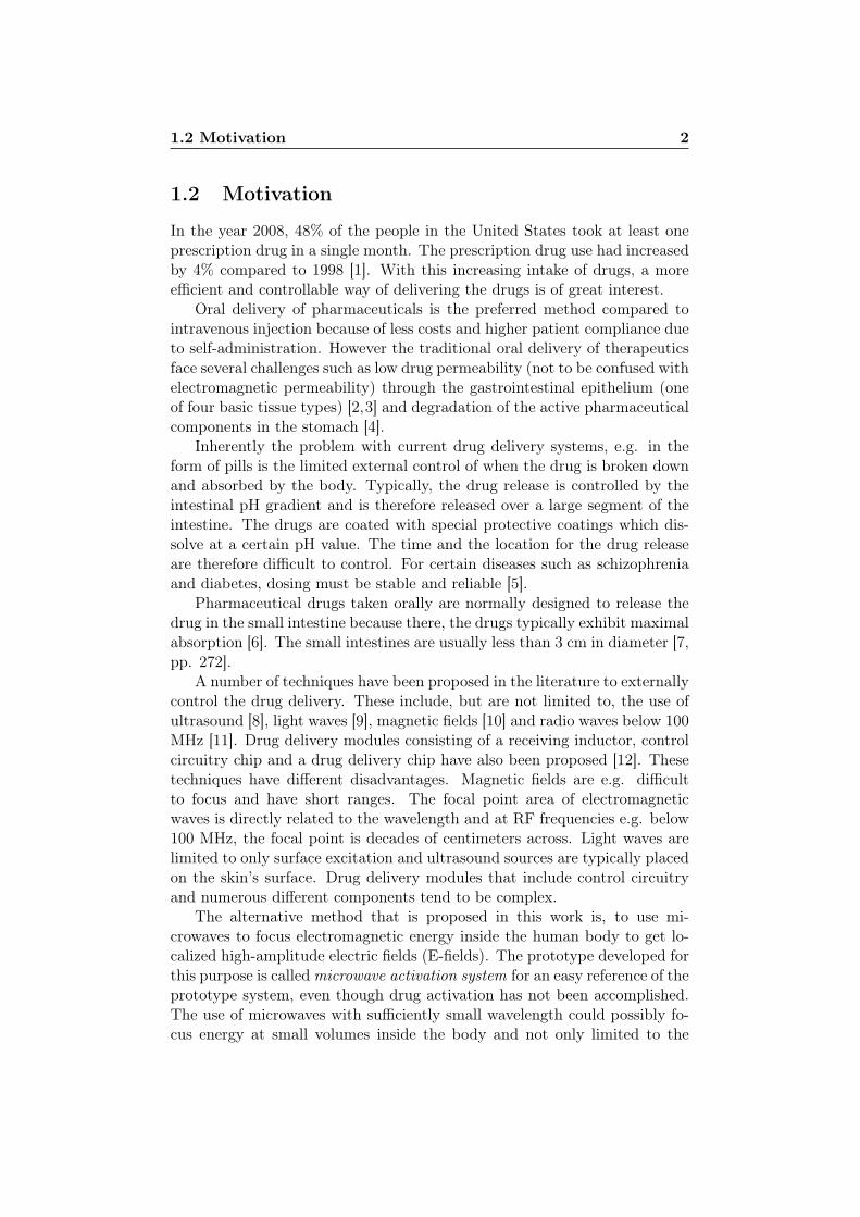
In the year 2008, 48% of the people in the United States took at least oneprescription drug in a single month. The prescription drug use had increasedby 4% compared to 1998 [1]. With this increasing intake of drugs, a moreefficient and controllable way of delivering the drugs is of great interest.
Oral delivery of pharmaceuticals is the preferred method compared tointravenous injection because of less costs and higher patient compliance dueto self-administration. However the traditional oral delivery of therapeuticsface several challenges such as low drug permeability (not to be confused withelectromagnetic permeability) through the gastrointestinal epithelium (oneof four basic tissue types) [2,3] and degradation of the active pharmaceuticalcomponents in the stomach [4].
Inherently the problem with current drug delivery systems, e.g. in theform of pills is the limited external control of when the drug is broken downand absorbed by the body. Typically, the drug release is controlled by theintestinal pH gradient and is therefore released over a large segment of theintestine. The drugs are coated with special protective coatings which dis-solve at a certain pH value. The time and the location for the drug releaseare therefore difficult to control. For certain diseases such as schizophreniaand diabetes, dosing must be stable and reliable [5].
Pharmaceutical drugs taken orally are normally designed to release thedrug in the small intestine because there, the drugs typically exhibit maximalabsorption [6]. The small intestines are usually less than 3 cm in diameter [7,pp. 272].
A number of techniques have been proposed in the literature to externallycontrol the drug delivery. These include, but are not limited to, the use ofultrasound [8], light waves [9], magnetic fields [10] and radio waves below 100MHz [11]. Drug delivery modules consisting of a receiving inductor, controlcircuitry chip and a drug delivery chip have also been proposed [12]. Thesetechniques have different disadvantages. Magnetic fields are e.g. difficultto focus and have short ranges. The focal point area of electromagneticwaves is directly related to the wavelength and at RF frequencies e.g. below100 MHz, the focal point is decades of centimeters across. Light waves arelimited to only surface excitation and ultrasound sources are typically placedon the skin’s surface. Drug delivery modules that include control circuitryand numerous different components tend to be complex.
The alternative method that is proposed in this work is, to use mi-crowaves to focus electromagnetic energy inside the human body to get lo-calized high-amplitude electric fields (E-fields). The prototype developed forthis purpose is calledmicrowave activation system for an easy reference of theprototype system, even though drug activation has not been accomplished.The use of microwaves with sufficiently small wavelength could possibly fo-cus energy at small volumes inside the body and not only limited to the
1.2 Motivation 3
surface. Microwaves do have their challenges in biological media, where oneof the most limiting factors is the inherent attenuation of the electromag-netic (EM) waves propagating in tissues with high water content, especiallymuscle tissues.
In order to efficiently utilize the received power despite this limitationcaused by tissues of high water content, specially designed micro-containers(also referred to as capsules) for pharmaceutical drugs is proposed in thiswork, to exploit the high-amplitude E-fields. The containers consist, amongother, of resonance circuits that are able to concentrate their received powerto localized areas on the capsule. This in turn, heats up parts of the con-tainers’ lid for the drug to be released.
Hyperthermia systems have been around for decades and their purposeis typically to heat up cancerous tissues in cancer treatment [13–36]. Non-invasive hyperthermia systems are similar to the microwave activation systemin the way that electromagnetic waves are to be transmitted into a humanbody and therefore many of the same principles apply in the microwaveactivation system as in non-invasive hyperthermia systems.
Non-invasive hyperthermia systems are meant to heat up cancerous tis-sues inside the body, which can result in prolonged exposure time of theperson to electromagnetic waves due to the body’s natural temperature reg-ulating abilities. Due to the heat, blood flow increases in the heated tissuewhich can improve the effectiveness of chemo- and radiation therapy. The mi-crowave activation system’s function also is to radiate electromagnetic wavesinto the human body, which inevitably causes some temperature increase.The main difference between known non-invasive hyperthermia systems andthe microwave activation system is that, the microwave activation system isto operate in the far-field of the transmitting antennas whereas the patientis typically situated in the near-field of hyperthermia applicators. The pro-posed micro-containers are specifically designed to respond to microwaves ata certain frequency that induce high-intensity E-fields with the help of thereceiving structure, which again induces localized heating in the containers.By the use of these containers, the idea is to try and avoid prolong heating ofthe body’s tissues while inducing enough heat in the containers themselvesto release the drug. No other external activation systems for drug releasebased on microwaves are currently known to the author.
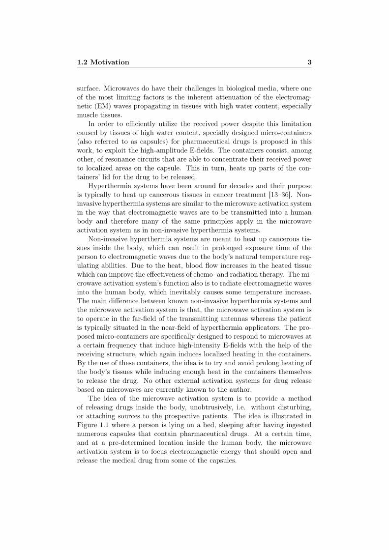
The idea of the microwave activation system is to provide a methodof releasing drugs inside the body, unobtrusively, i.e. without disturbing,or attaching sources to the prospective patients. The idea is illustrated inFigure 1.1 where a person is lying on a bed, sleeping after having ingestednumerous capsules that contain pharmaceutical drugs. At a certain time,and at a pre-determined location inside the human body, the microwaveactivation system is to focus electromagnetic energy that should open andrelease the medical drug from some of the capsules.
1.3 Thesis Overview 4
Figure 1.1: A person sleeping after ingesting drug capsules that arebeing activated by four external microwave applicators and drug isreleased.
1.3 Thesis Overview
The approach to this work was primarily practical, as the main purpose wasto develop and build an experimental microwave system which consists ofnumerous microwave and several non-microwave modules. This work wasstarted off by reviewing previous research on related topics such as hyper-thermia and wireless body area networks to find out what has been examinedbefore. The findings of the literature survey form, among other, the basisfor the design considerations in later chapters where the system is developedon both block- and module-level.
A fundamental theoretical description of electromagnetic (EM) proper-ties of biological media is considered essential to the understanding of awave behaviour in such media and is therefore presented in this thesis, asthe first topic after the literature survey. Wave transmission and reflectionat interfaces between two media, where at least one of the two media hasthe properties of a biological media is included as a part of the fundamentaltheoretical description.
1.3 Thesis Overview 5
In order to appropriately model human interaction with EM waves, hu-man tissue-like media must be fabricated for simulation purposes. The de-velopment of a suitable muscle tissue mimicking media is presented rightafter the description of EM properties of biological media due to its closerelation. Since no suitable media recipe that imitates muscle tissue seemedto exist in the literature, it was of high importance to develop such a recipein order to properly mimic human muscle tissue.
After the presentation of previous work in the literature, the theoreti-cal description of biological media properties and the creation of a mixturethat imitates muscle tissue, the system development is considered. The mi-crowave activation system that has the purpose of transmitting EM wavesinto a phantom was first designed at a block-level. There, e.g. the operat-ing frequency was chosen along with considerations on continuous wave vs.pulsed wave transmission. After the block-level design, the development ofeach individual block (module) of the system was performed. The chapter onmodule design and fabrication describes an extensive work done on numerousmicrowave modules. The design, fabrication and verification of each moduleis described in a relatively short manner since they are many and becauseseveral of these modules are designed using standard engineering techniques.Although some modules are described in a short manner, design and prac-tical fabrication effort is not reflected in the length of the description. Themost laborious work was done on the development of an antenna that hasthe ability to operate submerged in a muscle tissue mimicking medium andmaintain omnidirectional field distribution and it is therefore described in amore detailed manner.
When the development of the system had been finished, two kind ofexperimental setups were measured on. First, the wave transmission frominside a phantom and outwards was measured. The result from this setupprovides information on the wave propagation as measured by the receivers,while changing the source’s location inside the phantom. Secondly is a setupwhere several sources transmit simultaneously from the far-field of the phan-tom and radiate at the phantom in order to try and accomplish a focus pointinside the phantom. The wave behaviour encountered during these measure-ments is then discussed and more experiments to verify the explanationsgiven in the discussion, were performed.
As with any practical system, imperfections will to greater or less ex-tent affect the functionality of the system. Therefore, some of the essentialperformance-reduction factors are discussed after the measurement results.These factors are important to keep in mind while interpreting the measure-ments results.
Heating up a volume inside the body with microwaves as suggested inthe PhD project proposal was quickly found to be very challenging. The ideaof having a sensitive receiving structure attached to the drug-container thatreacts to EM fields which activates the drug release was therefore additionally
1.3 Thesis Overview 6
conceived. There was an encouragement to file a patent application for theidea, which was done and is currently in a PCT patent application stageat the European Patent Office. The concept of the receiving structure isdescribed at the end of this thesis in more details with simulation results.
A more detailed overview of the topic for each chapter is given below.
Chapter 2 presents a literature survey of prior research on the interac-tion of microwaves with the human body. Attention is primarily directed atthe field of hyperthermia and the field of wireless body area networks.
Chapter 3 begins with introducing the theory of biological tissues aslossy media. The behaviour of plane waves at the interfaces between twolossless media as well as between a lossless and a lossy media, such as anair - fat interface, is then examined. Attention is directed at the Brewsterangle and wave attenuation in biological media at oblique incident angles formaximizing power transfer into tissue.
The development of a suitable muscle tissue mimicking media is presentedin Chapter 4. A basic recipe is given, including only two ingredients. Animproved and a more complex recipe with three ingredients is furthermoregiven.
In Chapter 5 an overview of the microwave activation system is given. Theprinciple of operation is explained and the human torso phantom is pre-sented. The phantom is useful in verifying the functionality of the systemas well as to give an indication of the wave behaviour inside and aroundan actual human torso that, would be exposed to the microwave activationsystem’ waves. Various critical design-choices are discussed such as the eval-uation of the differences between continuous and pulsed waves. At the endof the chapter, designs are given for the mapping and the focusing opera-tions. These two cases describe a process of exiting EM waves from withinthe phantom as well as exiting EM waves from the outside of the phantom,respectively.
Chapter 6 presents the development of the individual modules that themicrowave activation system consists of. These include an antenna that isspecially developed for being submerged in a muscle tissue mimicking media,stacked patch antennas with extended bandwidth and controllable transmit-ters and receivers. Other microwave components such as a power amplifierthat ensures correct local oscillator drive and a 4-way power divider that hasa very good phase balance are also considered. Then the digital part is cov-ered which includes microcontroller boards, digital control, data acquisitionand the user interface for the PC.
1.3 Thesis Overview 7
In Chapter 7 the measurement results from the mapping operation are pre-sented. The behaviour of EM waves, which were transmitted from withinthe phantom and received externally to the phantom, are discussed and ex-planations about their behaviour are proposed.
Chapter 8 shows measurement results from the focusing operation. Fourexternal antennas were used to transmit EM waves towards a human torsophantom from a distance of about 0.7 m, arranged evenly around the phan-tom. An internal antenna, located inside the phantom was moved aroundin the phantom for amplitude measurements. Results from focusing of mi-crowaves inside the human torso phantom are presented.
Creeping waves are explained in Chapter 9 and their effect on focusingis discussed along with simulations that are carried out on a human voxelmodel. An experiment was performed to verify their presence.
Chapter 10 discusses several factors that need to be kept in mind whileoperating the microwave activation system and during interpretation of themeasured data. Some of these factors can result in performance-reductionof the overall system if not taken care of.
Chapter 11 deals with the development of a micro-container (capsule) thatis to hold pharmaceutical drugs until released. The capsule is proposed tobe equipped with a resonance circuit that, when mounted on a media withspecific EM properties, heats up a certain part of the capsule and releasesthe drug. Experiments were performed to determine what influence the ori-entation of the capsule has on its abilities to be excited by EM waves andby extension, release the medical drugs.
Chapter 12 summarizes the conclusions of the work that is presented here.
8
Chapter 2
Literature Survey
This chapter describes existing work on the influence of electromagneticwaves in and around a human body for medical or communication purposes.To the best of the author’s knowledge, no previous work exists on usingelectromagnetic waves in the microwave region for external drug activationpurposes. The topics that are considered are hyperthermia in cancer treat-ment and the use of wireless body area network. Both of these topics dealwith electromagnetic waves inside the human body or close to the surface ofthe body.
2.1 Hyperthermia
Hyperthermia has been shown to be effective, especially when combinedchemo- and radio-therapy, in the treatment against cancer [37, 38]. As pre-viously noted, non-invasive hyperthermia systems are used to heat up can-cerous tissues in the body without penetrating the body. Hyperthermiautilized various frequencies such as 40 MHz [13], 60 MHz [15], 100 MHz [14],140 MHz [16, 17], 433 MHz [18–22], 520 MHz [23], 630 MHz [24], 915 MHz[25–32] and 2.45 GHz [33–36].
Phased arrays have been the most popular setups for non-invasive hy-perthermia systems due to the ability of focusing [13, 13, 14, 16–18, 20, 22,25–27, 31, 33, 36, 39–48]. In order to measure the E-fields inside or on thesurface of phantoms and as a feedback signal for adaptive array, typically annon-perturbing E-field probe have been used. [14,49,50].
High power transmitters have been used with phased arrays to increasethe temperature up to 6C for up to several hours. Power levels of 35W [31],40W [16], 100W [26,27], 150W [18,22], 175W [51], 300W [25], 500W [14,20]and 860W [52] have been shown in the literature. Several of the systems makeuse of a water bolus, which typically contain de-ionized water to couple theelectromagnetic energy into the patient and therefore avoid large reflections[14,20,22,27,29,34,41,53].
2.2 Wireless Body Area Network 9
Several attempts have been made to measure the effects of the phasedarray non-invasive hyperthermia systems in regards to temperature distribu-tion mapping. The most precise technique is claimed to be MRI (MagneticResonance Imaging) [54, 55]. However other methods have also been pre-sented for this purpose such as presented in [51,56] or [57] for phantoms. Anon-perturbing temperature probe is presented in [58] which can be used,with negligible disturbance of the E-field.
Various types of applicators have been presented in the literature fornon-invasive hyperthermia systems. These include dipole antennas [14, 17,21, 35, 42], end-loaded dipole antennas [16], square applicators [25], induc-tive current sheet applicators [59], microstrip spiral antennas [27], microstrippatch antennas [41,59], parabolic reflectors [60], helical radiators [13], waveg-uide antennas [34, 59, 61] and metal-plate lens applicators that are found toradiate 2 times deeper than a regular waveguide antenna [20].
There is a fine line when irradiating tissues between heating it, withoutdamaging the tissue and causing a definite injury. Research has shown thatwhen heating tissue to 43.5C for 40 minutes, no injury is presented butwhen heated for 60 minutes, major damage occurs [62]. By heating to hightemperatures, prolonged heating time can be avoided [63]. Time can bedecreased by a factor of two for every single degree increase in temperature[26].
Variations in physical parameters [64, 65] such as e.g. fat thickness canhave big influence on the appearance of hot spots in the fat layer and themuscle layer underneath [24,53].
Both single antenna array ring structures or multiple ring structures havebeen presented in the literature. In general, the ability to focus and avoidhot spots, which appear at least above 250 MHz [66], are improved with morethan one ring [48]. With increasing number of radiators, power optimizationgets improved [17, 18, 45, 67]. By implementing adaptive nulling techniques,hot spots in healthy tissues can be reduced significantly [52,55,68]. Reportsalso exist of the possibility of using broadband signals to focus electromag-netic waves and reduce hot spots [23,69], although mostly for low loss breasttissue.
2.2 Wireless Body Area Network
Wireless body area network (WBAN) consist of a number of wireless devicesthat communicate with each other and are either wearable or implantable inthe human body. This can, e.g. be a single wireless sensor inside the bodythat communicates to an outside network such as a local area network, or anumber of sensors on the body communicating with each other. The termwireless body-centric communications describes the communication methodbetween modules located in and around the body.
2.2 Wireless Body Area Network 10
There are three scenarios for wireless body-centric communications, wherethe two most relevant will be covered below:
• Off-body, where a device located on a body communicates with one ormore devices located off-body (not covered here).
• On-body, where a number of devices located on the body communicatewith each other.
• In-body, where some (or all) of the devices are implanted in the body,rather than worn (e.g. pace-makers).
Over the last few years, the interest of WBANs has grown significantlyand common applications of WBANs are within medicine, military, sportsand multimedia. Writings by T.G. Zimmerman at IBM gave the field ofpersonal area networks or, the more common, body area networks a lift intothe current form [70,71]. Today, sensors are often placed in shoes of runnersthat can communicate with their mobile devices which makes a completerecording of the pace, distance, time elapsed and calories burned duringthe workout [72]. Wrist watches can record heart-rate while receiving GPSsignals from satellites for accurate positioning [73]. For diagnosing sleepingdisorders, a compact device is attached on the body to measure among otherEEG, ECG and EMG signals and transmits the signals in real time overBluetooth to a tablet or a personal computer to be diagnosed [74].
Sensor modules are often simply connected to a standard off-the-shelfwireless module for transmitting and receiving the necessary data withoutgiving too much considerations to propagation paths or the influence of thebody on the antenna. These standard wireless modules typically supportwidespread technologies such as Bluetooth, WLAN or Zigbee and are usedfor simplicity and to ensure reliable data transfer [75,76]. Bluetooth, WLANand Zigbee operate in the license-free band between 2.4 and 2.5 GHz. Fur-thermore, Zigbee also operates at 868 MHz and 915 MHz bands [77]. Arecently allocated band, the so-called MICS (Medical Implant Communica-tion System) band, operating between 402 and 405 MHz is mainly aimed atcommunication between medical implants and external transceivers. Thisband is, however, limited to maximum EIRP of -16 dBm since the frequencyband is shared with the METAIDS meteorological system [78].
The power consumptions of the sensors and wireless devices is one of thebiggest concern in WBANs. The size and weight of the unit is at a largepart determined by the battery required to supply current to the circuits.The running time of the unit is also determined by the battery size, since itis directly related to the power consumption. For these reasons, it can beessential to reduce power consumption as much as possible. The efficiencyof the transmit and receive antenna as well as the ability to predict thepropagation behaviour from or on the body are of high importance, especiallywhen determining wave propagation path and attenuation of a system.
2.2 Wireless Body Area Network 11
2.2.1 On-Body Communication
Transmitting from one place on the surface of the body to another placeon the surface of the body is called on-body communication. Transmissionpaths can e.g. be direct line of sight or, the transmitter and the receivercan be on opposite sides of the body. For the line-of-sight case the propa-gation is simpler than when the path is a curved path, a reflecting path ora combination of both. The human body essentially acts as a wave guid-ing structure [79] which allows for curved paths. An example of this is inhearing aids where a person has one hearing aid in each ear and one de-vice transmits data to the other hearing aid to obtain stereo sound effect inboth ears [80]. Propagation model for the human head can e.g. be foundin [81] whereas a conventional dual-slope model can be obtained to providean on-body propagation model for the human body as a function of distancein [82].
A challenging part of any on-body system is the antenna design. Anantenna placed on the skin of a person can experience detuning in reso-nance frequency and change in gain pattern [77, 83]. The electromagneticproperties of the skin varies from person to person and things such as in-creased perspiration can change the conductivity of the skin and thereforethe antenna properties. Some on-body antennas [84,85] show decreased effi-ciency of between 40% and 90% when placed on a phantom simulating muscletissue [86]. Specialized antennas have been manufactured to excite creepingwaves specifically for transmission along the curvature of the body in [87].According to [88], in order to match the characteristics of the creeping waves,the on-body antennas must be vertically polarized with an end-fire patternalong the body surface.
2.2.2 In-Body Communication
Transmitting from a source inside the body and outwards to an external re-ceiver and vice versa is known as in-body communication. Inductive couplingis the most commonly used technique for communicating with implanted de-vices, due to its simplicity and deep penetration into the human body owingto the non-magnetic properties of the body. Inductive coupling has typicallyvery short range which requires the external transceiver to be touching theperson [78]. A longer communication range can be achieved by operatingat higher frequencies since that gives rise to propagating electromagneticwaves. This also improves the bandwidth and therefore higher bitrates canbe realized.
The propagation behaviour of electromagnetic waves inside the humanbody is complicated to model due to the numerous different tissue typesand variations in the human form between every individual. There have,however, been advances in this area over the last decade or so.
2.2 Wireless Body Area Network 12
The creation of a propagation model for wireless body area networksstarted with [89] for small dipole antennas inside the body which have beenfurther developed, e.g. in [90] where simulations and measurements are com-pared for a homogeneous phantom. Propagation models using heterogeneousmodels have since been introduced [91, 92]. Experiments with propagationmodels outside the body have also been presented [93]
A general limitation of transmitting data from within the human body isthe signal to noise ratio (SNR) at the receiver’s end. Faster data-rates callfor wider bandwidth which often mean higher operating frequencies and withhigher frequencies, power attenuation increases in human tissues, thus reduc-ing the received signal power. More advanced modulation schemes than theclassical QPSK (Quadrature Phase-Shift Keying) and FSK (Frequency-ShiftKeying) are not considered practical in the case of medical implants as theyrequire more data processing capabilities and are more power consuming.QPSK and FSK, however, require positive SNR in order to operate satisfac-tory [78]. Selection of the operating frequency not only determines the powerattenuation in tissue due to tissue conductivity’s frequency dependence, butit also determines the free-space path loss. This path loss is one of the largestsingle loss factors of the propagating wave between an implanted source anda transceiver external to the body and ultimately greatly influences the SNR.Beside selecting the optimal frequency, by increasing the transmitting power,the gains of the transmitting and receiving antennas as well as increasing thereceiver’s sensitivity are measures of increasing the SNR. The most effectiveand perhaps simple action could however be, to simply bring the transmitterand the receiver physically closer to each other, if possible.
Variations in implant situations can have high impact on propagationmodels. For example, when dealing with propagation models of implants inmoving patients, transmitting to a stationary receiver at a distance from thepatient, additional margin, due to fading, should be taken into a considera-tion to account for reflections in the patient’s room [78, 94]. When dealingwith an implant in a patient’s stomach, there is a difference in whether thepatient has recently eaten or not that has to be accounted for. Wave at-tenuation is shown to be greater and steeper if a radiator is placed insidean empty stomach (radiator surrounded with air) compared to a full stom-ach [95, 96]. When examining the effect of varying frequency close to theimplanted source, revealing results appear. In [95] a drop in the E-field ofapproximately 90 dB, relative to the source, is seen within 7 centimetresfrom the source, almost independent of the frequency. This is suggested tobe due to the quasi-static E-field’s dependence on distance rather than fre-quency. Also it is noted that generally the average received signal decreaseslogarithmically with distance as expected.
2.3 Discussion 13
2.3 Discussion
The objective of this work is to examine the possibility of using microwavesfor external activation of drug release. The project description from Chapter1 provides the guidelines for this work and must be followed. Beside theseguidelines, I imposed a requirement as well which is that, the system shalloperate in the far-field. Ultimately, the idea is that drug release inside thebody can be activated externally for the convenience of the patient. Thisincludes, but is not limited to, release of medicine during the night while thepatient is sleeping. For this reason, only an unobtrusive system is consideredas a possibility in this work. Even though this requirement poses a significantchallenge to transmit sufficient power into the human body, it also simplifieswave propagation analysis.
Hyperthermia systems are treatment systems where patients are typicallyplaced in the near-field of the applicators. This reduces the effect of pathloss which is inevitable in systems that operate in the far-field. The powerlevels of hyperthermia systems are not applicable in the microwave activationsystem as the objective is not to heat tissue and maintain high temperaturesover a period of time, rather it is to excite a receiving structure on a drugcapsule.
Several hyperthermia systems utilize water bolus that is placed at thesurface of the patient’s skin. The transmitting antennas are typically sub-merged in this water bolus. This is done because from theory predictionsand previous research, large wave reflections at air - skin interface have beenobserved. A theoretical analysis is performed on wave propagation at inter-faces typical for the human body in Chapter 3, where a method of maximumtransmission of power into the body is also suggested.
According to the literature, the number of antennas and the number ofring structures around the patient improves the ability to focus and reduceshot spots outside the focus point. However, a certain degree of simplicityhad to be maintained and therefore four sources were considered sufficientto provide a proof-of-principle setup.
The operating frequency of the microwave activation system was chosento be around 2.45 GHz. A number of phased-array hyperthermia systemshave been reported to operate at this frequency, some specially designed fordeep-seated tumour irradiation. Smaller wavelength of the operating sys-tem ensures narrower focus point, but the losses also increase with higherfrequency and therefore it was a matter of compromise. The choice of op-erating frequency was ultimately decided based on the practicality of theavailability of microwave components since for an entire system, numerousdifferent components were required. A discussion on the choice of operatingfrequency is covered in further detail in Chapter 5.
As presented above, inductive coupling is the most commonly used tech-nique for communicating with implanted devices which is rarely operated at

2.3 Discussion 14
microwave frequencies. The literature of wireless body area networks largelycovers only standard wireless modules such as Bluetooth, WLAN and Zigbeeand generally not much consideration is given to the actual microwave part.There are, however, several reported cases where the propagation behaviourof EM waves inside the human body has been modelled, both for homo-geneous and heterogeneous phantoms. The homogeneous model predictsapproximately 5 dB power attenuation for every centimeter in muscle.
15
Chapter 3
Electromagnetic Properties ofBiological Media
In this chapter, the electromagnetic properties of lossy media such as bi-ological tissues are examined. Also the transmission and the reflection atboundaries of air and fat are studied for determining the power transfer intoa body or a phantom.
3.1 Lossy Biological Media
Losses in media such as biological tissues are a consequence of a finite andnon-zero conductivity. The conductivity typically contains both static andfrequency dependent components that result in a current flow when an E-field is applied.
∇×H = Jc + Jd, (3.1)
is one of Maxwell’s equations and shows the relation between the magneticfield intensity,H and the two current densities in a source-free lossy dielectricmedia. Jc is the conduction current density which represents flow of electronsand holes and Jd is the displacement current density. The relation betweenthe conduction current and the electric field intensity, E, is
Jc = σsE, (3.2)
where σs is the static conductivity (DC-conductivity) in [S/m]. Similarly forthe displacement current and the electric flux density, D, the relation is
Jd = jωD, (3.3)
where ω is the angular frequency and can be represented by the frequency,f, ω = 2πf .
3.1 Lossy Biological Media 16
The electric flux density and the electric field intensity are linked throughthe complex permittivity, ε with:
D = εE. (3.4)
The complex permittivity has, as the name indicates, a real part and animaginary part and is represented by
ε = ε′ − jε′′ = ε0(ε′r − jε′′r), (3.5)
where ε0 is the permittivity of vacuum (8.854 ·10−12 F/m), ε′r is the real part(often referred to as the relative dielectric constant) and ε′′r is the imaginarypart of the relative permittivity.
The magnitude of the real part is directly related to the medium’s abil-ity to store E-field whereas the imaginary part represents the losses in themedium as a result of an oscillating E-field.
By inserting (3.2) through (3.5) into (3.1) the result is
∇×H = σsE + jω(ε′ − jε′′)E (3.6)
= (σs + ωε′′)E + jωε′E (3.7)
= σeE + jωε′E, (3.8)
where σe is the effective conductivity and is given by
σe = σs + ωε′′. (3.9)
The effective conductivity is frequency dependent and includes bothlosses due to conduction current as well as losses due to displacement cur-rent. The effective conductivity is used throughout this work and will beinterchangeably referred to as the effective conductivity or simply the con-ductivity. Materials that often are nearly lossless at DC, such as deionizedwater that has σs = 0.0001 S/m [97] become lossy at microwave frequencies.At 2.45 GHz e.g., the conductivity is σe = 1.35 S/m for deionized water andthe losses are almost solely due to the displacement current.
Table 3.1 lists examples of relative permittivity and conductivity valuesfor some typical biological tissues at 2.45 GHz [98,99].
The complex propagation constant γ is composed of α and β and theirrelationship is
γ = α+ jβ. (3.10)
The propagation constant describes the phase change and attenuation ofa travelling wave in a lossy medium.

3.1 Lossy Biological Media 17
Table 3.1: Typical relative permittivity and effective conductivityfor biological tissues at 2.45 GHz.
Tissue ε′r σe [S/m]
Fat 5.28 0.10
Bone 15.0 0.60
Skin 38.0 1.46
Brain 42.5 1.51
Muscle 53.6 1.81
Wave attenuation in media is dependent on σe and ε′r and is representedusing the attenuation constant by [100, pp. 139]
α = ω√µε′
1
2
[√1 +
( σeωε′
)2− 1
] 12
, (3.11)
where µ is the permeability. All parameters are that of the media. Thepermeability of biological tissue is approximately the same as that of vacuumand can therefore be directly replaced by µ0 = 4π · 10−7 H/m [101, pp. 33].In a lossless media σe is zero and therefore α becomes zero as well. Thephase constant, β, is similarly [100, pp. 139]
β = ω√µε′
1
2
[√1 +
( σeωε′
)2+ 1
] 12
. (3.12)
Table 3.2 shows α and β of skin, fat and muscle at 2.45 GHz, based onε′r and σe from Table 3.1. As can be seen, the attenuation in every cm ofmuscle is very close to the attenuation in a cm of skin, or approximately 4dB, which can be found by multiplying α with 0.08686 [97].
Table 3.2: Typical attenuation constants and phase constants forbiological tissues at 2.45 GHz along with the wavelength in the tissue.
Tissue α αdB β λ
[Np/m] [dB/cm] [rad/m] [cm]
Muscle 46.24 4.01 378.67 1.7
Fat 15.29 1.33 169.55 5.3
Skin 44.31 3.85 319.57 2.0
3.2 Transmission and Reflection at Interfaces 18
3.2 Transmission and Reflection at Interfaces
Radiating electromagnetic waves at a human torso for the purpose of havingpower penetrating into a tissue efficiently, requires considerations about wavebehaviour at interfaces between two media. Attention is directed at theair-fat interface which analogous to the experimental setup to be presentedin Chapter 5. This kind of interface can cause large reflections, thus lowpenetration of power.
Electromagnetic waves that are traveling from air (media 1) across anair-fat interface are partially reflected at the interface and the rest is trans-mitted into the fat (media 2). The levels of the reflected and the transmittedwaves depend upon the respective permittivities and conductivities as wellas the polarization and the incidence angle of the field. This will be furtherexplained in the next sections.
3.2.1 Lossless - Lossless Interface
Biological tissues such as muscle and skin can be considered as a interme-diate conductive media, on the low conductive end. A good dielectric is amedia that fulfils (σ/ωε′) 1 and a good conductor as a media that fulfils(σ/ωε′) 1 [100, pp. 74-75].
At 2.45 GHz, muscle has e′r = 53.6 and σ = 1.81 S/m [98] which gives(σ/ωε′) = 0.25. Disputably, 0.25 is not much less than 1 and thereforemuscle is categorized here as a intermediate conductive media. Fat is ingeneral slightly lossy, with (σ/ωε′) = 0.14 and can be categorized as eithera intermediate conductive media or as a good dielectric. In this section,lossless fat is defined as a medium that has similar permittivity to fat butwith zero conductivity. The simplification of a lossless fat in this section is forillustrating the transmission and reflection behaviour at a air-fat boundaryin approximate manner.
In Figure 3.1, two media with a planar interface are shown for two po-larization cases. Media 1 (air) has the permittivity ε1 and permeability µ1and media 2 (fat) has correspondingly ε2 and µ2. The conductivities σ1, σ2are 0 S/m as both media are considered lossless for now.
If there is an incident uniform TEM (transverse electromagnetic) wavetravelling from air into a fat at an incident angle, θi, in respect to the normalto the planar interface of the two media, part of the wave gets reflected whilethe rest is transmitted into the lossless fat. The plane of the interface lies inthe x-y plane and the normal vector out of media 2, n, is in the negative zdirection.
The incident wave can be split into a linearly polarized perpendicularcomponent and a parallel component, as shown in Figure 3.1(a) and 3.1(b),respectively. A perpendicular polarized wave has the E-field vector perpen-dicular to the plane created by the direction vector of the incident wave,
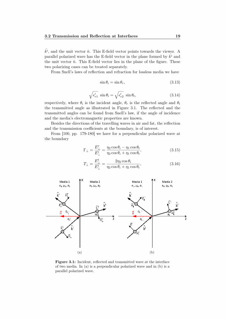
3.2 Transmission and Reflection at Interfaces 19
ki, and the unit vector n. This E-field vector points towards the viewer. Aparallel polarized wave has the E-field vector in the plane formed by ki andthe unit vector n. This E-field vector lies in the plane of the figure. Thesetwo polarizing cases can be treated separately.
From Snell’s laws of reflection and refraction for lossless media we have
sin θi = sin θr, (3.13)
√ε′r1 sin θi =
√ε′r2 sin θt, (3.14)
respectively, where θi is the incident angle, θr is the reflected angle and θtthe transmitted angle as illustrated in Figure 3.1. The reflected and thetransmitted angles can be found from Snell’s law, if the angle of incidenceand the media’s electromagnetic properties are known.
Besides the directions of the travelling waves in air and fat, the reflectionand the transmission coefficients at the boundary, is of interest.
From [100, pp. 179-180] we have for a perpendicular polarized wave atthe boundary
Γ⊥ =Er⊥Ei⊥
=η2 cos θi − η1 cos θtη2 cos θi + η1 cos θt
, (3.15)
T⊥ =Et⊥Ei⊥
=2η2 cos θi
η2 cos θi + η1 cos θt, (3.16)
(a) (b)
Figure 3.1: Incident, reflected and transmitted wave at the interfaceof two media. In (a) is a perpendicular polarized wave and in (b) is aparallel polarized wave.
3.2 Transmission and Reflection at Interfaces 20
(a) (b)
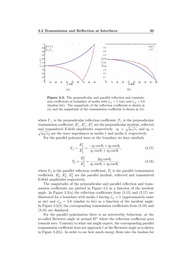
Figure 3.2: The perpendicular and parallel reflection and transmis-sion coefficients at boundary of media with ε′r1 = 1 (air) and ε′r2 = 5.8(lossless fat). The magnitude of the reflection coefficient is shown in(a) and the magnitude of the transmission coefficient is shown in (b).
where Γ⊥ is the perpendicular reflection coefficient, T⊥ is the perpendiculartransmission coefficient, Ei⊥, E
r⊥, E
t⊥ are the perpendicular incident, reflected
and transmitted E-field amplitudes respectively. η1 =√µ1/ε1 and η2 =√
µ2/ε2 are the wave impedances in media 1 and media 2, respectively.For the parallel polarized wave at the boundary we have similarly
Γ‖ =Er‖
Ei‖=−η1 cos θi + η2 cos θtη1 cos θi + η2 cos θt
, (3.17)
T‖ =Et‖
Ei‖=
2η2 cos θiη1 cos θi + η2 cos θt
, (3.18)
where Γ‖ is the parallel reflection coefficient, T‖ is the parallel transmissioncoefficient, Ei‖, E
r‖ , E
t‖ are the parallel incident, reflected and transmitted
E-field amplitudes respectively.The magnitudes of the perpendicular and parallel reflection and trans-
mission coefficients are plotted in Figure 3.2 as a function of the incidentangle. In Figure 3.2(a) the reflection coefficients from (3.15) and (3.17) areillustrated for a boundary with media 1 having ε′r1 = 1 (approximately sameas air) and ε′r2 = 5.8 (similar to fat) as a function of the incident angle.In Figure 3.2(b) the corresponding transmission coefficients from (3.16) and(3.18) are displayed.
For the parallel polarization there is an noteworthy behaviour, at theso-called Brewster angle at around 67 where the reflection coefficient goestowards zero. Contrary to what one might expect, the corresponding paralleltransmission coefficient does not approach 1 at the Brewster angle as is shownin Figure 3.2(b). In order to see how much energy flows into the lossless fat

3.2 Transmission and Reflection at Interfaces 21
in the parallel case, the power transmission coefficient, TPWR‖ , is found. The
time-averaged power densities for the incident, reflected and transmittedplane waves are
~Si =1
2R~Ei × ~H i∗
=
1
2η1
∣∣Ei∣∣2 ki, (3.19)
~Sr =1
2R~Er × ~Hr∗
=
1
2η1|Er|2 kr, (3.20)
~St =1
2R~Et × ~Ht∗
=
1
2η2
∣∣Et∣∣2 kt, (3.21)
respectively. The energy that is incident on a unit area of the interface of thetwo media is the normal component of the power density vector. This alsoapplies to the energies propagating away from the interface, the reflectedand transmitted power densities. This results in
n · ~Si = − 1
2η1
∣∣Ei∣∣2 cos θi, (3.22)
n · ~Sr =1
2η1|Er|2 cos θr, (3.23)
n · ~St = − 1
2η2
∣∣Et∣∣2 cos θt, (3.24)
where the minus signs of the incident and transmitted waves are due to thefact that their respective k vectors are in the opposite direction to the vectornormal to media 2, n.
The power transmission coefficient, TPWR‖ can now be found as
TPWR‖ =
n · ~Stn · ~Si
=η1
∣∣∣Et‖∣∣∣2
cos θt
η2
∣∣∣Ei‖∣∣∣2
cos θi
=
√ε′r2ε′r1
cos θtcos θi
∣∣T‖∣∣2 , (3.25)
as well as the power reflection coefficient
ΓPWR‖ =
n · ~Srn · ~Si
=η1
∣∣∣Er‖∣∣∣2
cos θr
η1
∣∣∣Ei‖∣∣∣2
cos θi
=∣∣Γ‖∣∣2 , (3.26)
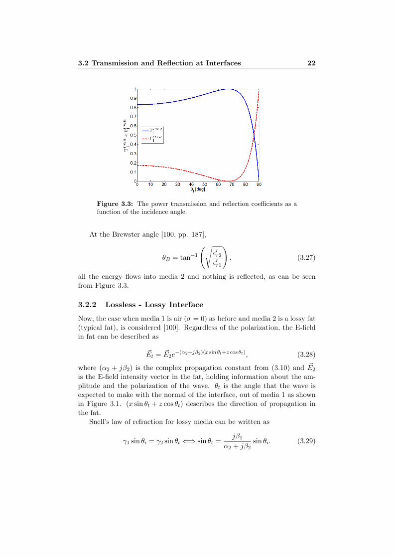
since from Snell’s law of reflection, (3.13), θi = θr.Figure 3.3 illustrates the parallel power transmission and reflection co-
efficients as a function of the incidence angle at the boundary of two mediahaving ε′r1 = 1 and ε′r2 = 5.8, as before.
3.2 Transmission and Reflection at Interfaces 22
Figure 3.3: The power transmission and reflection coefficients as afunction of the incidence angle.
At the Brewster angle [100, pp. 187],
θB = tan−1
(√ε′r2ε′r1
), (3.27)
all the energy flows into media 2 and nothing is reflected, as can be seenfrom Figure 3.3.
3.2.2 Lossless - Lossy Interface
Now, the case when media 1 is air (σ = 0) as before and media 2 is a lossy fat(typical fat), is considered [100]. Regardless of the polarization, the E-fieldin fat can be described as
~Et = ~E2e−(α2+jβ2)(x sin θt+z cos θt), (3.28)
where (α2 + jβ2) is the complex propagation constant from (3.10) and ~E2
is the E-field intensity vector in the fat, holding information about the am-plitude and the polarization of the wave. θt is the angle that the wave isexpected to make with the normal of the interface, out of media 1 as shownin Figure 3.1. (x sin θt + z cos θt) describes the direction of propagation inthe fat.
Snell’s law of refraction for lossy media can be written as
γ1 sin θi = γ2 sin θt ⇐⇒ sin θt =jβ1
α2 + jβ2sin θi. (3.29)

3.2 Transmission and Reflection at Interfaces 23
Using cos2 θt + sin2 θt = 1, we can write
cos θt =
√1−
(jβ1
α2 + jβ2
)2
sin2θi = s(cos ζ + j sin ζ), (3.30)
where s(cos ζ + j sin ζ) is a vector in the complex plane since θt is clearly acomplex angle, indicating a non-uniform wave. Inserting (3.30) and (3.29)into (3.28), ~Et can now be written as
~Et = ~E2e−(α2+jβ2)
(x
jβ1α2+jβ2
sin θi+zs(cos ζ+j sin ζ)). (3.31)
The jβ1α2+jβ2
term from (3.30) can be rewritten as
jβ1α2 + jβ2
· α2 − jβ2α2 − jβ2
=
a︷ ︸︸ ︷β1β2
α22 + β22
+j
b︷ ︸︸ ︷β1α2
α22 + β22
, (3.32)
where a represents the real part and b the imaginary part. (3.30) can nowbe rewritten as
cos θt =
√1−
(a2 + j2ab− b2
)sin2θi, (3.33)
and combining s(cos ζ + j sin ζ) from (3.30) and (3.33), cos2 θt becomes
cos2 θt = s2(cos ζ + j sin ζ)2 (3.34)
= s2
cos 2ζ︷ ︸︸ ︷(cos2 ζ − sin2 ζ) +js2
sin 2ζ︷ ︸︸ ︷2(cos ζ sin ζ) (3.35)
= 1− a2 sin2 θi + b2 sin2 θi − j2ab sin2 θi. (3.36)
From (3.35) and (3.36) the real parts must be equal, thus
s2 cos 2ζ = 1− (a2 − b2) sin2 θi, (3.37)
and the imaginary parts as well
s2 sin 2ζ = −2ab sin2 θi. (3.38)
An effort to simplify the argument in the exponential of (3.31) yields
− (α2 + jβ2)
(x
jβ1α2 + jβ2
sin θi + zs(cos ζ + j sin ζ)
)
= −x(aα2 − bβ2) sin θi − jx(bα2 + aβ2) sin θi
− zα2e︷ ︸︸ ︷
s(α2 cos ζ − β2 sin ζ)−jzq︷ ︸︸ ︷
s(α2 sin ζ + β2 cos ζ), (3.39)
3.2 Transmission and Reflection at Interfaces 24
where we define s(α2 cos ζ − β2 sin ζ) as the effective attenuation constant,α2e and s(α2 sin ζ + β2 cos ζ) as q, for ease of reference.
Examining the (aα2 − bβ2) factor from (3.39) closer results in
(aα2 − bβ2) =β1β2
α22 + β22
α2 −β1α2
α22 + β22
β2 = 0. (3.40)
Likewise, the (bα2 + aβ2) factor can be replaced by β1 since
a =bβ2α2
, (3.41)
and
b =β1α2
α22 + β22
⇐⇒ β1 = bα2 +bβ22α2
, (3.42)
which results in
β1 = bα2 + aβ2. (3.43)
Using the results from (3.39), (3.40) and (3.43), (3.31) can be written as
~Et = ~E2e−zα2e · e−j(xβ1 sin θi+zq). (3.44)
The first thing to notice about the result in (3.44) is that the transmittedwave is indeed a non-uniform wave since the planes of constant amplitude andplanes of constant phases do not coincide. It is noteworthy that the waveis only attenuated in the z-direction, regardless of the angle of incidence.In principle, it means that when the resulting wave is travelling in somedirection in the x-z plane, as is the case here, only the travel in z-direction willcause attenuation. The magnitude of the attenuation is, however, dependenton the angle of incident. The resulting angle of transmission and the effectivephase constant are
ψt = tan−1(β1 sin θi
q
), (3.45)
β2e =√
(β1 sin θi)2 + q2, (3.46)
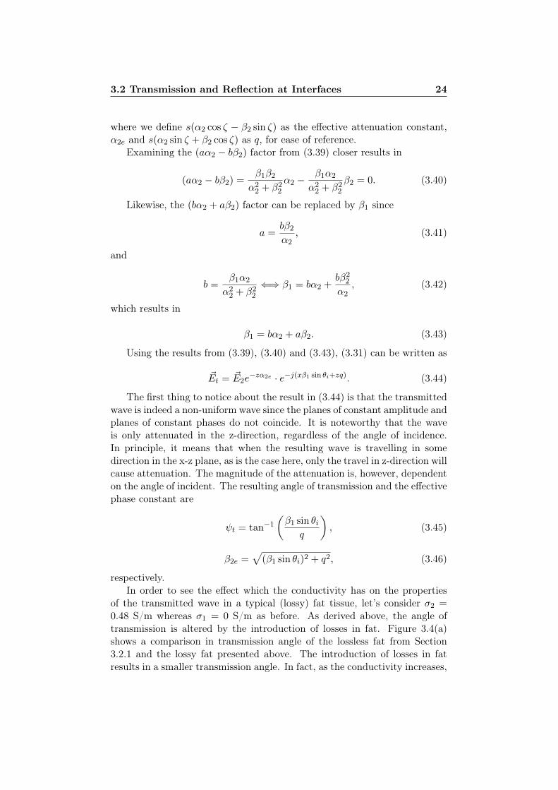
respectively.In order to see the effect which the conductivity has on the properties
of the transmitted wave in a typical (lossy) fat tissue, let’s consider σ2 =0.48 S/m whereas σ1 = 0 S/m as before. As derived above, the angle oftransmission is altered by the introduction of losses in fat. Figure 3.4(a)shows a comparison in transmission angle of the lossless fat from Section3.2.1 and the lossy fat presented above. The introduction of losses in fatresults in a smaller transmission angle. In fact, as the conductivity increases,
3.2 Transmission and Reflection at Interfaces 25
(a) (b)
Figure 3.4: In (a) the angle of transmission for lossless and interme-diate conductive media is shown. In (b) the phase constant of media2 along with the effective phase constant of a travelling wave in lossymedia at an oblique angle is shown.
the transmission angle approaches 0, since there can not exist a tangentialE-field in a perfect electrical conductor. Figure 3.4(b) illustrates how theconductivity slightly alters the behaviour of the phase constant in fat whichbecomes dependent on the incident angle in the lossy fat. This is also truefor the effective attenuation constant, α2e.
As will become evident later in this work, the ε′r2 and σ2 values repre-senting fat, actually are the measured values for a media that emulates theelectromagnetic properties of fat in the microwave activation system (dis-cussed in Appendix B).
3.2.3 Maximum Power Transfer into Tissue
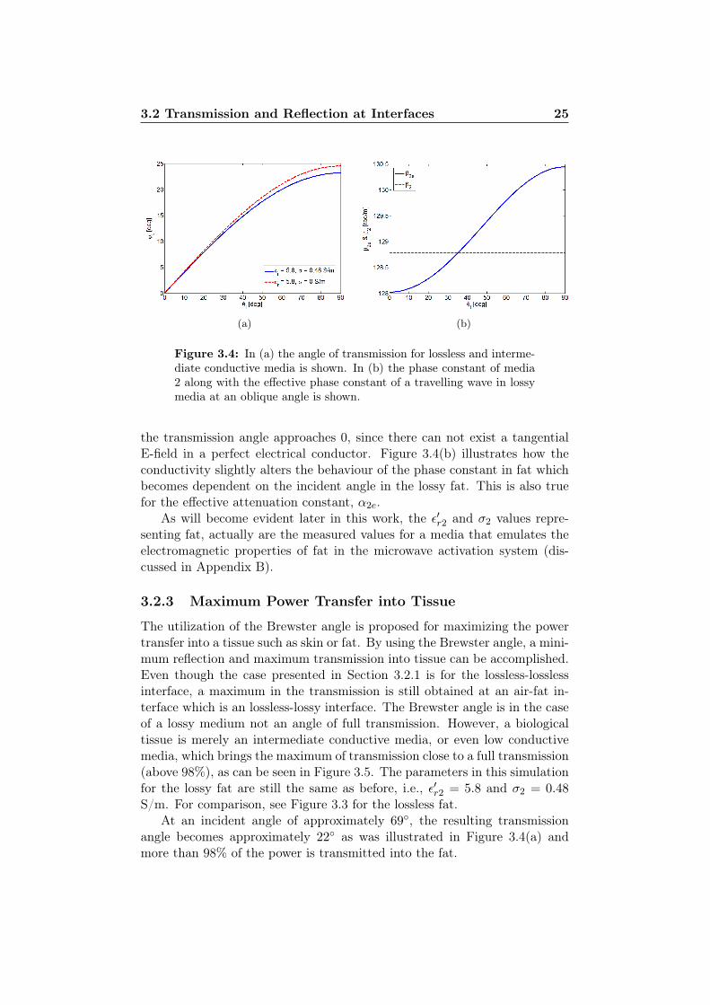
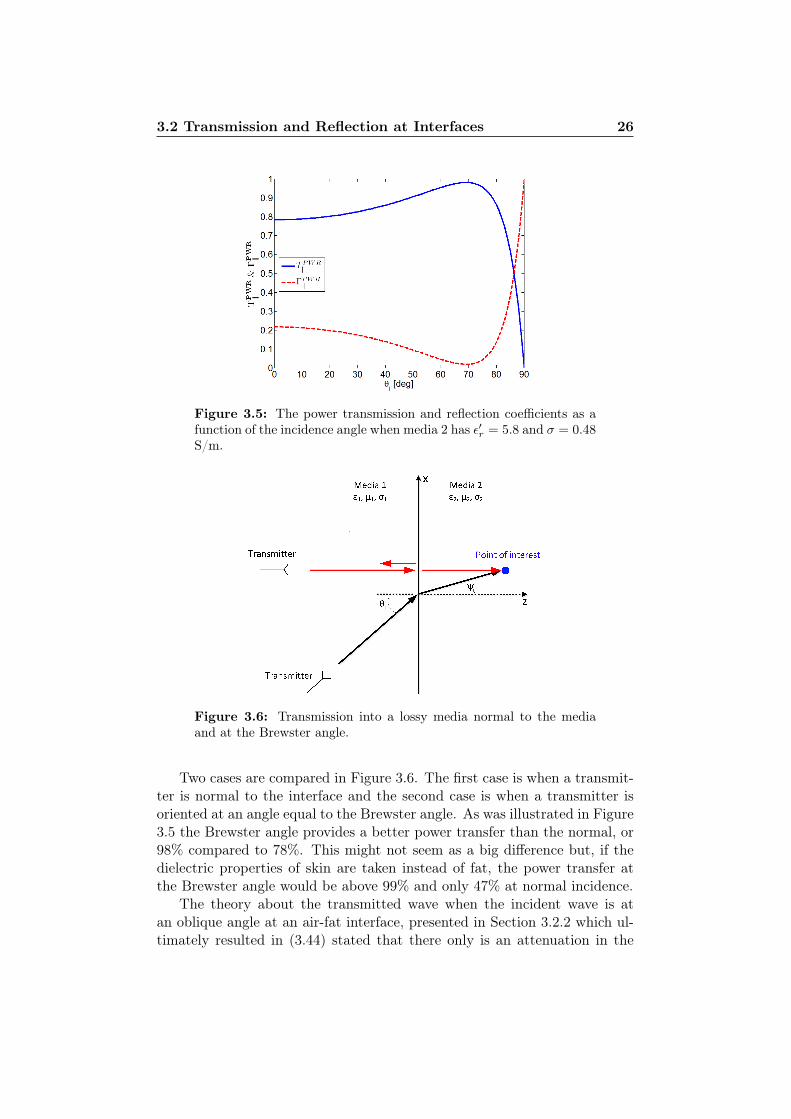
The utilization of the Brewster angle is proposed for maximizing the powertransfer into a tissue such as skin or fat. By using the Brewster angle, a mini-mum reflection and maximum transmission into tissue can be accomplished.Even though the case presented in Section 3.2.1 is for the lossless-losslessinterface, a maximum in the transmission is still obtained at an air-fat in-terface which is an lossless-lossy interface. The Brewster angle is in the caseof a lossy medium not an angle of full transmission. However, a biologicaltissue is merely an intermediate conductive media, or even low conductivemedia, which brings the maximum of transmission close to a full transmission(above 98%), as can be seen in Figure 3.5. The parameters in this simulationfor the lossy fat are still the same as before, i.e., ε′r2 = 5.8 and σ2 = 0.48S/m. For comparison, see Figure 3.3 for the lossless fat.
At an incident angle of approximately 69, the resulting transmissionangle becomes approximately 22 as was illustrated in Figure 3.4(a) andmore than 98% of the power is transmitted into the fat.
3.2 Transmission and Reflection at Interfaces 26
Figure 3.5: The power transmission and reflection coefficients as afunction of the incidence angle when media 2 has ε′r = 5.8 and σ = 0.48S/m.
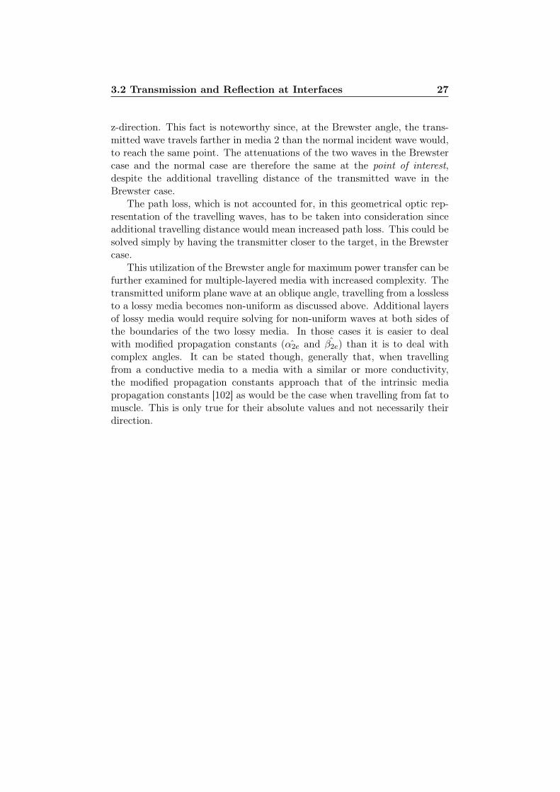
Figure 3.6: Transmission into a lossy media normal to the mediaand at the Brewster angle.
Two cases are compared in Figure 3.6. The first case is when a transmit-ter is normal to the interface and the second case is when a transmitter isoriented at an angle equal to the Brewster angle. As was illustrated in Figure3.5 the Brewster angle provides a better power transfer than the normal, or98% compared to 78%. This might not seem as a big difference but, if thedielectric properties of skin are taken instead of fat, the power transfer atthe Brewster angle would be above 99% and only 47% at normal incidence.
The theory about the transmitted wave when the incident wave is atan oblique angle at an air-fat interface, presented in Section 3.2.2 which ul-timately resulted in (3.44) stated that there only is an attenuation in the
3.2 Transmission and Reflection at Interfaces 27
z-direction. This fact is noteworthy since, at the Brewster angle, the trans-mitted wave travels farther in media 2 than the normal incident wave would,to reach the same point. The attenuations of the two waves in the Brewstercase and the normal case are therefore the same at the point of interest,despite the additional travelling distance of the transmitted wave in theBrewster case.
The path loss, which is not accounted for, in this geometrical optic rep-resentation of the travelling waves, has to be taken into consideration sinceadditional travelling distance would mean increased path loss. This could besolved simply by having the transmitter closer to the target, in the Brewstercase.
This utilization of the Brewster angle for maximum power transfer can befurther examined for multiple-layered media with increased complexity. Thetransmitted uniform plane wave at an oblique angle, travelling from a losslessto a lossy media becomes non-uniform as discussed above. Additional layersof lossy media would require solving for non-uniform waves at both sides ofthe boundaries of the two lossy media. In those cases it is easier to dealwith modified propagation constants (α2e and β2e) than it is to deal withcomplex angles. It can be stated though, generally that, when travellingfrom a conductive media to a media with a similar or more conductivity,the modified propagation constants approach that of the intrinsic mediapropagation constants [102] as would be the case when travelling from fat tomuscle. This is only true for their absolute values and not necessarily theirdirection.

28
Chapter 4
Muscle Tissue MimickingMedia Development
4.1 Introduction
For experimental setups of the interaction of microwaves and biologicaltissue, phantoms are traditionally used as the equivalent of a biological tissue.Phantoms are designed to have similar electromagnetic properties as a hu-man, within a specific frequency range. Depending on the complexity of aphantom, it can consist of one or more different tissue mimicking media.
Several different types of phantom recipes have been proposed throughthe years such as [103–110]. Phantoms are often made from solid materialsand high viscous gels that are optically non-transparent. These kinds ofphantoms are preferred when they have to take a certain form, such as a legor a head because they do not easily lose their original shape with time andcan be cast in the required form. These kind of phantoms, however, cannotaccommodate for free movements of measurement probes inside the media.One of the most important tissue type to mimic accurately is the muscle asit is one of the main cause of EM wave attenuation in the body and also itconstitutes a large part of the human body.
4.2 Reference Medium
The most utilized muscle tissue mimicking media recipe for 2.45 GHz waspresented by Chou et al. [103] and was therefore a possible candidate for thiswork. Its viscous properties were, however, undocumented and unknown.The recipe was followed and the resulting electromagnetic properties mea-sured.
The mixture was fabricated from deionized water, household salt (NaCl),polyethylene powder (<20 µm diameter) and TX-151. When mixing to-gether, the salt was first dissolved in the water, a drop of dishwashing liquid
4.2 Reference Medium 29
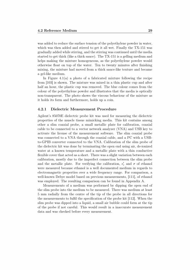
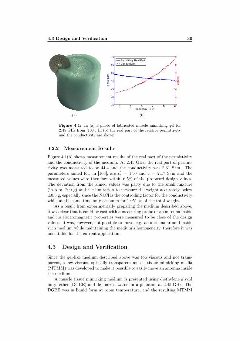
was added to reduce the surface tension of the polyethylene powder in water,which was then added and stirred to get it all wet. Finally the TX-151 wasgradually added while stirring, and the stirring was continued until the mediastarted to get thick (like a thick sauce). The TX-151 is a gelling medium andhelps making the mixture homogeneous, as the polyethylene powder wouldotherwise float on top of the water. Ten to twenty minutes after finishingmixing, the mixture had moved from a thick sauce-like texture and becamea gel-like medium.
In Figure 4.1(a) a photo of a fabricated mixture following the recipefrom [103] is shown. The mixture was mixed in a thin plastic cup and afterhalf an hour, the plastic cup was removed. The blue colour comes from thecolour of the polyethylene powder and illustrates that the media is opticallynon-transparent. The photo shows the viscous behaviour of the mixture asit holds its form and furthermore, holds up a coin.
4.2.1 Dielectric Measurement Procedure
Agilent’s 85070E dielectric probe kit was used for measuring the dielectricproperties of the muscle tissue mimicking media. This kit contains amongother a slim coaxial probe, a small metallic plate for calibration, coaxialcable to be connected to a vector network analyzer (VNA) and USB key toactivate the license of the measurement software. The slim coaxial probewas connected to a VNA through the coaxial cable, and a PC with a USB-to-GPIB converter connected to the VNA. Calibration of the slim probe ofthe dielectric kit was done by terminating the open end using air, de-ionizedwater at a known temperature and a metallic plate with a thin conductiveflexible cover that acted as a short. There was a slight variation between eachcalibration, mostly due to the imperfect connection between the slim probeand the metallic plate. For verifying the calibration, ε′r and σ of ethanolwere measured because ethanol is a well documented medium in regards toelectromagnetic properties over a wide frequency range. For comparison, awell-known Debye model based on previous measurements, [111], of ethanolwas employed. The resulting comparison can be found in Appendix A.
Measurements of a medium was performed by dipping the open end ofthe slim probe into the medium to be measured. There was medium at least5 mm radially from the centre of the tip of the probe in all directions forthe measurements to fulfil the specification of the probe kit [112]. When theslim probe was dipped into a liquid, a small air bubble could form at the tipof the probe if not careful. This would result in a inaccurate measurementdata and was checked before every measurement.
4.3 Design and Verification 30
(a)
1 2 3 4 5 610
20
30
40
50
60
70
ε r rea
l par
tFrequency [GHz]
1 2 3 4 5 60
1
2
3
4
5
6
σ [S
/m]
Permittivity Real PartConductivity
(b)
Figure 4.1: In (a) a photo of fabricated muscle mimicking gel for2.45 GHz from [103]. In (b) the real part of the relative permittivityand the conductivity are shown.
4.2.2 Measurement Results
Figure 4.1(b) shows measurement results of the real part of the permittivityand the conductivity of the medium. At 2.45 GHz, the real part of permit-tivity was measured to be 44.4 and the conductivity was 2.31 S/m. Theparameters aimed for, in [103], are ε′r = 47.0 and σ = 2.17 S/m and themeasured values were therefore within 6.5% of the proposed design values.The deviation from the aimed values was party due to the small mixture(in total 200 g) and the limitation to measure the weight accurately below±0.5 g, especially since the NaCl is the controlling factor for the conductivitywhile at the same time only accounts for 1.051 % of the total weight.
As a result from experimentally preparing the medium described above,it was clear that it could be cast with a measuring probe or an antenna insideand its electromagnetic properties were measured to be close of the designvalues. It was, however, not possible to move, e.g. an antenna around insidesuch medium while maintaining the medium’s homogeneity, therefore it wasunsuitable for the current application.
4.3 Design and Verification
Since the gel-like medium described above was too viscous and not trans-parent, a low-viscous, optically transparent muscle tissue mimicking media(MTMM) was developed to make it possible to easily move an antenna insidethe medium.
A muscle tissue mimicking medium is presented using diethylene glycolbutyl ether (DGBE) and de-ionized water for a phantom at 2.45 GHz. TheDGBE was in liquid form at room temperature, and the resulting MTMM
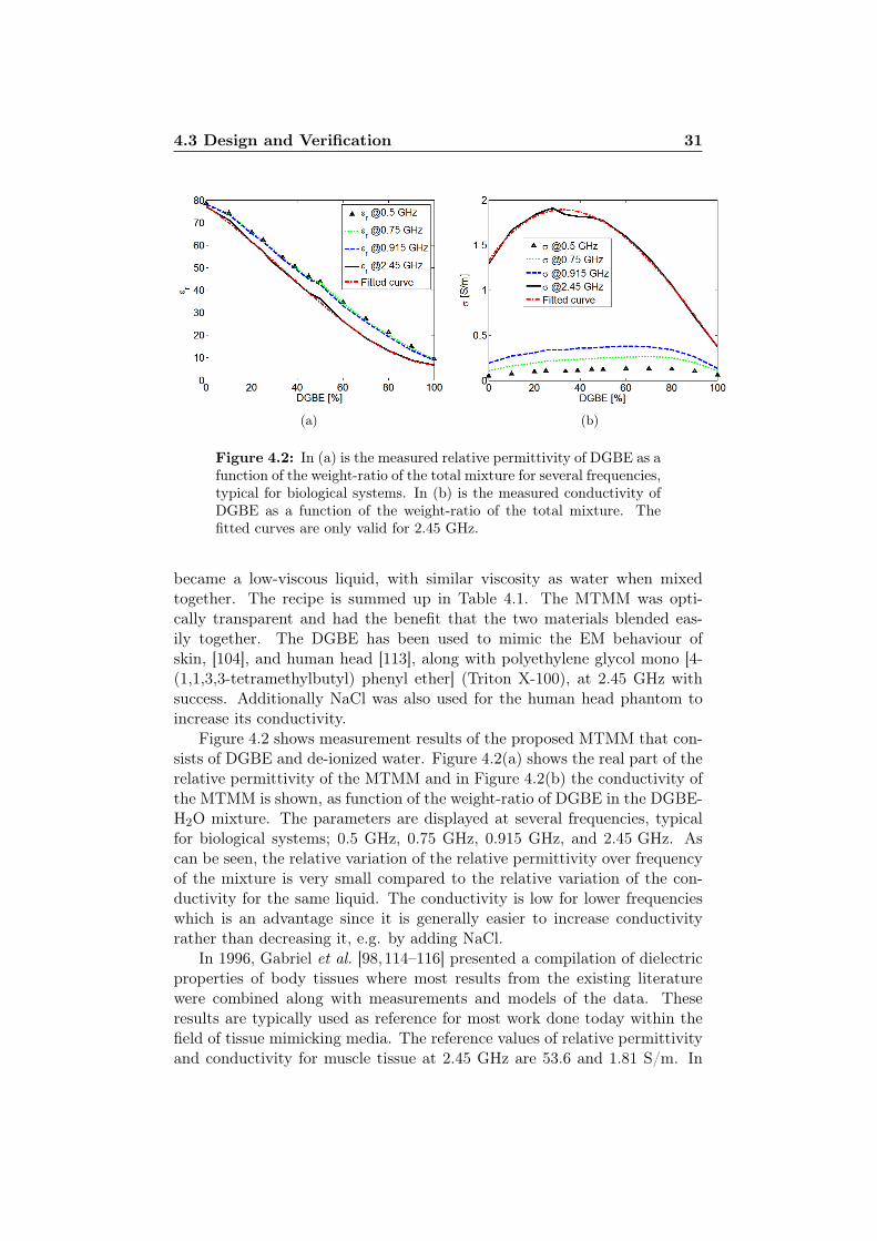
4.3 Design and Verification 31
(a) (b)
Figure 4.2: In (a) is the measured relative permittivity of DGBE as afunction of the weight-ratio of the total mixture for several frequencies,typical for biological systems. In (b) is the measured conductivity ofDGBE as a function of the weight-ratio of the total mixture. Thefitted curves are only valid for 2.45 GHz.
became a low-viscous liquid, with similar viscosity as water when mixedtogether. The recipe is summed up in Table 4.1. The MTMM was opti-cally transparent and had the benefit that the two materials blended eas-ily together. The DGBE has been used to mimic the EM behaviour ofskin, [104], and human head [113], along with polyethylene glycol mono [4-(1,1,3,3-tetramethylbutyl) phenyl ether] (Triton X-100), at 2.45 GHz withsuccess. Additionally NaCl was also used for the human head phantom toincrease its conductivity.
Figure 4.2 shows measurement results of the proposed MTMM that con-sists of DGBE and de-ionized water. Figure 4.2(a) shows the real part of therelative permittivity of the MTMM and in Figure 4.2(b) the conductivity ofthe MTMM is shown, as function of the weight-ratio of DGBE in the DGBE-H2O mixture. The parameters are displayed at several frequencies, typicalfor biological systems; 0.5 GHz, 0.75 GHz, 0.915 GHz, and 2.45 GHz. Ascan be seen, the relative variation of the relative permittivity over frequencyof the mixture is very small compared to the relative variation of the con-ductivity for the same liquid. The conductivity is low for lower frequencieswhich is an advantage since it is generally easier to increase conductivityrather than decreasing it, e.g. by adding NaCl.
In 1996, Gabriel et al. [98,114–116] presented a compilation of dielectricproperties of body tissues where most results from the existing literaturewere combined along with measurements and models of the data. Theseresults are typically used as reference for most work done today within thefield of tissue mimicking media. The reference values of relative permittivityand conductivity for muscle tissue at 2.45 GHz are 53.6 and 1.81 S/m. In
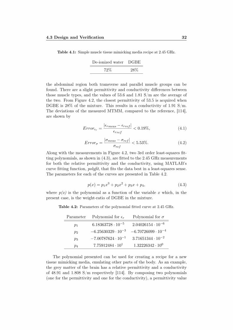
4.3 Design and Verification 32
Table 4.1: Simple muscle tissue mimicking media recipe at 2.45 GHz.
De-ionized water DGBE
72% 28%
the abdominal region both transverse and parallel muscle groups can befound. There are a slight permittivity and conductivity differences betweenthose muscle types, and the values of 53.6 and 1.81 S/m are the average ofthe two. From Figure 4.2, the closest permittivity of 53.5 is acquired whenDGBE is 28% of the mixture. This results in a conductivity of 1.91 S/m.The deviations of the measured MTMM, compared to the reference, [114],are shown by
Errorεr =|εrmeas − εrref |
εrref< 0.19%, (4.1)
Errorσ =|σmeas − σref |
σref< 5.53%. (4.2)
Along with the measurements in Figure 4.2, two 3rd order least-squares fit-ting polynomials, as shown in (4.3), are fitted to the 2.45 GHz measurementsfor both the relative permittivity and the conductivity, using MATLAB’scurve fitting function, polyfit, that fits the data best in a least-squares sense.The parameters for each of the curves are presented in Table 4.2.
p(x) = p1x3 + p2x
2 + p3x+ p4, (4.3)
where p(x) is the polynomial as a function of the variable x which, in thepresent case, is the weight-ratio of DGBE in the mixture.
Table 4.2: Parameters of the polynomial fitted curve at 2.45 GHz.
Parameter Polynomial for εr Polynomial for σ
p1 6.18363728 · 10−5 2.04026154 · 10−6
p2 −6.25630329 · 10−3 −6.70726099 · 10−4
p3 −7.00787624 · 10−1 3.71651344 · 10−2
p4 7.75912484 · 101 1.32226342 · 100
The polynomial presented can be used for creating a recipe for a newtissue mimicking media, emulating other parts of the body. As an example,the grey matter of the brain has a relative permittivity and a conductivityof 48.91 and 1.808 S/m respectively [114]. By composing two polynomials(one for the permittivity and one for the conductivity), a permittivity value
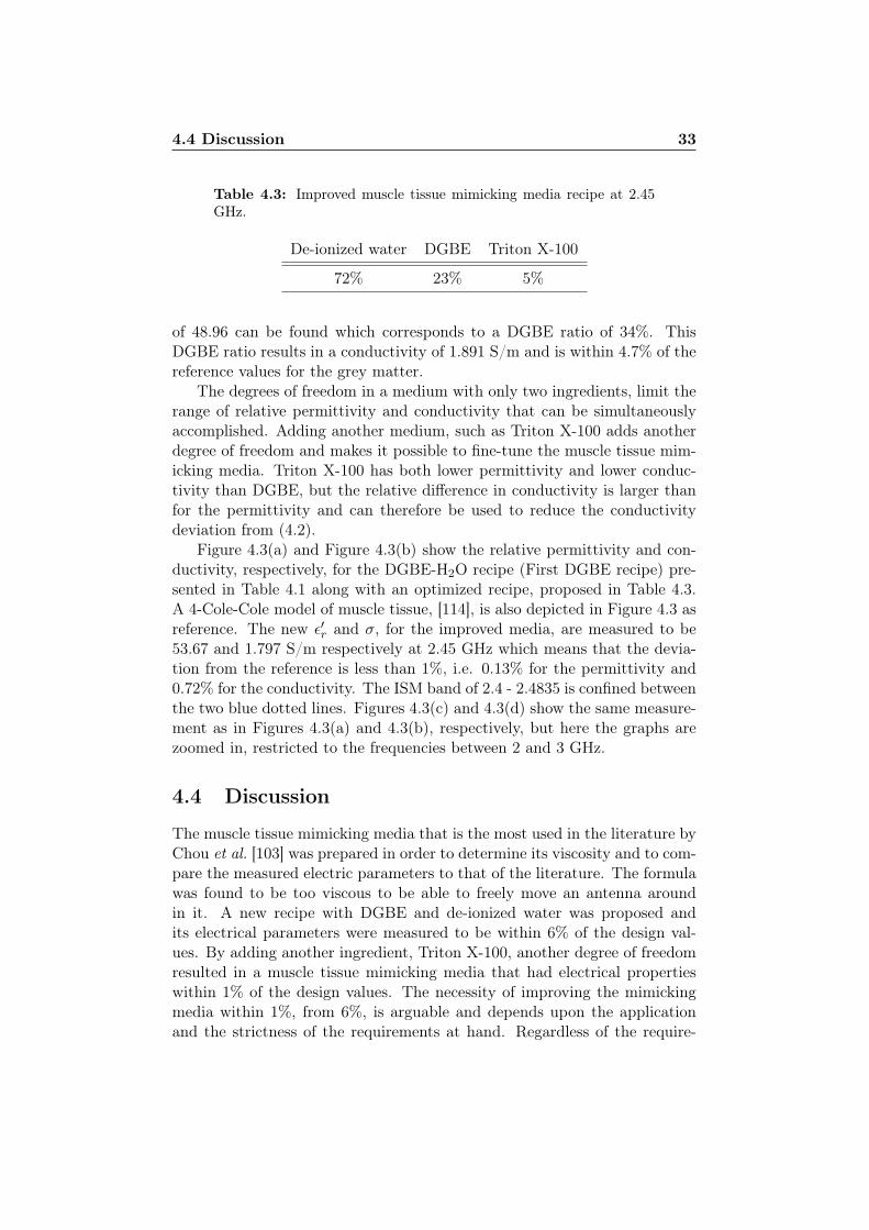
4.4 Discussion 33
Table 4.3: Improved muscle tissue mimicking media recipe at 2.45GHz.
De-ionized water DGBE Triton X-100
72% 23% 5%
of 48.96 can be found which corresponds to a DGBE ratio of 34%. ThisDGBE ratio results in a conductivity of 1.891 S/m and is within 4.7% of thereference values for the grey matter.
The degrees of freedom in a medium with only two ingredients, limit therange of relative permittivity and conductivity that can be simultaneouslyaccomplished. Adding another medium, such as Triton X-100 adds anotherdegree of freedom and makes it possible to fine-tune the muscle tissue mim-icking media. Triton X-100 has both lower permittivity and lower conduc-tivity than DGBE, but the relative difference in conductivity is larger thanfor the permittivity and can therefore be used to reduce the conductivitydeviation from (4.2).
Figure 4.3(a) and Figure 4.3(b) show the relative permittivity and con-ductivity, respectively, for the DGBE-H2O recipe (First DGBE recipe) pre-sented in Table 4.1 along with an optimized recipe, proposed in Table 4.3.A 4-Cole-Cole model of muscle tissue, [114], is also depicted in Figure 4.3 asreference. The new ε′r and σ, for the improved media, are measured to be53.67 and 1.797 S/m respectively at 2.45 GHz which means that the devia-tion from the reference is less than 1%, i.e. 0.13% for the permittivity and0.72% for the conductivity. The ISM band of 2.4 - 2.4835 is confined betweenthe two blue dotted lines. Figures 4.3(c) and 4.3(d) show the same measure-ment as in Figures 4.3(a) and 4.3(b), respectively, but here the graphs arezoomed in, restricted to the frequencies between 2 and 3 GHz.
4.4 Discussion
The muscle tissue mimicking media that is the most used in the literature byChou et al. [103] was prepared in order to determine its viscosity and to com-pare the measured electric parameters to that of the literature. The formulawas found to be too viscous to be able to freely move an antenna aroundin it. A new recipe with DGBE and de-ionized water was proposed andits electrical parameters were measured to be within 6% of the design val-ues. By adding another ingredient, Triton X-100, another degree of freedomresulted in a muscle tissue mimicking media that had electrical propertieswithin 1% of the design values. The necessity of improving the mimickingmedia within 1%, from 6%, is arguable and depends upon the applicationand the strictness of the requirements at hand. Regardless of the require-
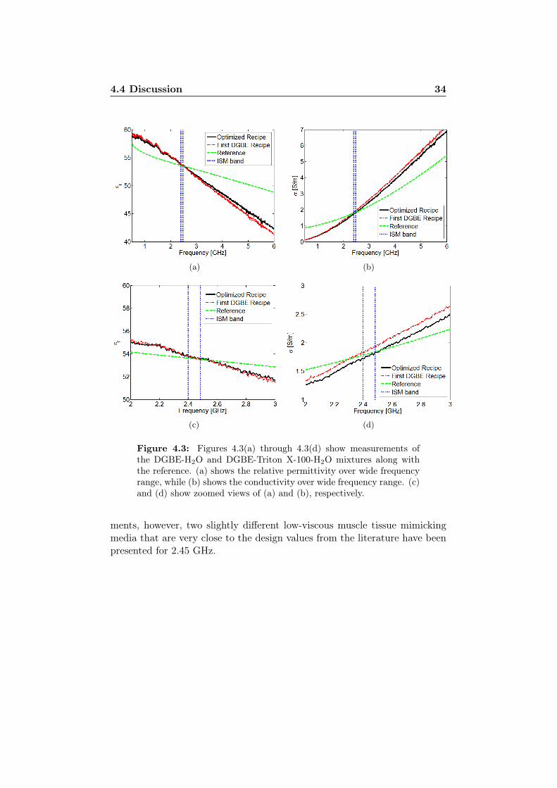
4.4 Discussion 34
(a) (b)
(c) (d)
Figure 4.3: Figures 4.3(a) through 4.3(d) show measurements ofthe DGBE-H2O and DGBE-Triton X-100-H2O mixtures along withthe reference. (a) shows the relative permittivity over wide frequencyrange, while (b) shows the conductivity over wide frequency range. (c)and (d) show zoomed views of (a) and (b), respectively.
ments, however, two slightly different low-viscous muscle tissue mimickingmedia that are very close to the design values from the literature have beenpresented for 2.45 GHz.
35
Chapter 5
Microwave Activation System -Overview
5.1 Introduction
Constructive interference of electromagnetic waves were proposed in Chapter1 as the method to be utilized in the microwave activation system. Multiplesuperimposed waves that are in phase, add together creating a focus point.There are a number of critical design-choices to be made in a system thatis to radiate electromagnetic waves inside the human body. These includeoperating frequency, number and location of antennas, pulsed vs. continuouswave, power level and flexibility of the system.
Generally with increasing frequency, attenuation in biological tissues in-creases and makes it more challenging to penetrate deeper into the body.With higher frequency, due to its smaller wavelength it is, however, possibleto focus onto smaller volumes. Components such as antennas can be madesmaller and that impacts the overall size of the system as well as the far-fieldregion.
The most similar systems that focus electromagnetic waves inside thehuman body are non-invasive electromagnetic hyperthermia systems. Thesesystems are able to illuminate the surface or the sub-surface of a body partin order to heat up a specific volume. The heat is usually applied to regionsin the body that contain a cancerous tissue for the purpose of increasingchemo- and radiation therapy’s effectiveness. Hyperthermia systems havebeen made, utilizing various frequencies, typically within any of the ISMbands between 40 MHz and 2.45 GHz.
The two most often used frequencies within hyperthermia throughout theyears have been 433 MHz and 915 MHz. There have been several publica-tions regarding selection of the optimal frequency for penetrating deep intobiological tissue. The suggested frequencies are among others 1.5 GHz [117]and 1 GHz [118]. Practical matters such as the size of the radiating an-
5.1 Introduction 36
tennas, availability of components at the operating frequency and cost alsoaffect the choice of frequency. Typically the physical size of the antennaneeds to be around one half the operating wavelength. Antennas that aresmaller than that tend to have reduced efficiency. In general, with increasingfrequency the focus point inside the tissue becomes smaller. The half-powerspot size at the focal depth is around 3/4 of the wavelength in diameter [43].The conductivity of biological tissue also increases with higher frequencies,as was shown in Section 4, resulting in higher power loss. A trade-off there-fore has to be made when selecting the operating frequency. As stated inChapter 2, the operating frequency of the current microwave activation sys-tems is chosen to be 2.45 GHz mainly because the required components arereadily available. The fact that the antennas can be relatively small sizedand the predicted focus area is smaller than it would be at lower frequenciesare also good qualities. Limited existing research on the topic, at 2.45 GHzalso makes it interesting to examine and perhaps supplement to the existingresearch, if possible. The system is designed to cover a bandwidth of 100MHz, i.e. from 2.4 to 2.5 GHz to cover the ISM band and more importantly,to allow for manufacturing deviations.
The process of typical medication such as orally ingested pills as describedin Chapter 1, has its difficulties. The introduction to a microwave activa-tion system for drug release is to offer an alternative solution to standarddrug delivery mechanisms. The goal is to deliver drugs without presentinga restrain to a person. That means that strapping a person with a belt ofantennas or having a person lie in a specially made bench where bags ofwater are placed on the person could be avoided. A drug delivery system ofthat kind would almost defeat the purpose of its existence if a person needsto strap on a belt every time they need a dose of medicine, instead of justtaking a pill or having an injection.
Having an unobtrusive microwave activation system inherently causesseveral issues. One of the issues is the power coupling from air to the tissue.Air has a relative permittivity close to 1 and coupling into a tissue that hasa relative permittivity of 38 - 53, depending on the type of tissue, causesa high reflection at the boundary. As was presented in Section 3.2.3, thereflected power of a normal incident plane wave is approximately 53% (-3.3dB) of the incident power, making less than half of the transmitted powerenter into the tissue. It is however worth mentioning that a reflection loss of3.3 dB is equivalent to losses that would occur in less than 0.9 cm of extramuscle thickness. Variation of muscle mass between individuals can easilybe beyond 0.9 cm, hence the reflection loss is not a dominant factor.
Another important issue is the path loss that occurs in travelling waves.The path loss decreases the power density with distance from the radiatingantenna. The farther the radiating antennas are from the target, the lesspower is radiated onto the target.
5.2 Operating Principle 37
5.2 Operating Principle
The experimental setup for microwave activation consists of four antennas,a simple dual-layered cylindrical phantom, a single antenna operating insidethe phantom, four transmitters, four receivers, two frequency synthesizers, adriver amplifier, three power dividers along with a PC and data acquisitionhardware. The outer layer of the phantom represents fat layer of a humanand the inner layer represents a muscle layer.
The principle of operation for the experimental setup is twofold. First,an antenna that is operating inside of a phantom (internal antenna) is con-nected to a single transmitter and radiates EM waves from within the phan-tom and outwards. Receivers are connected to four external antennas. Theabsolute and relative amplitudes and phases, respectively, at the locations ofthe external antennas are measured and collected using the data acquisitionhardware along with the PC. This is referred to as mapping.
In the second part of operation, each of the four external antennas areconnected to their own transmitter. Their relative amplitudes and phasesare set to obtain constructive interference and hence a focus point. Theinternal antenna are used, connected to a single receiver, measuring thetotal amplitude received. This is referred to as focusing.
Focusing in this case can be considered the reciprocal of the mappingsince the phantommedia, as well as real biological tissues, are linear, isotropicand, with certain approximation, time-invariant media. For the experimen-tal setup for microwave activation, Lorentz’s reciprocity principle can be uti-lized, since the system fulfils the requirement for a reciprocal system [100, pp.323]. The Lorentz’s reciprocity principle can be written, when the fields areobserved in the far field and the sources are in the same medium, as follows
∫∫∫
V( ~E1 · ~J2 − ~H1 · ~M2)dv
′ =
∫∫∫
V( ~E2 · ~J1 − ~H2 · ~M1)dv
′, (5.1)
where ~J and ~M are electric and magnetic sources, respectively. ~E1 and ~H1
are the electric and magnetic field intensities, respectively, that are generatedby ~J1 and ~M1. Similarly, ~E2 and ~H2 are generated by ~J2 and ~M2. Assumingthat we have no magnetic sources we get
∫∫∫
V( ~E1 · ~J2)dv′ =
∫∫∫
V( ~E2 · ~J1)dv′. (5.2)
This form of reduced Lorentz’s reciprocity theorem (5.2) states is that ife.g. a current density at location 1 generates an E-field at location 2, anotherequal current source which is at location 2, will generate the same E-field atlocation 1.
This essentially means that the forward transmission coefficient S21 hasto be equal to the reverse transmission coefficient S12 for a system where
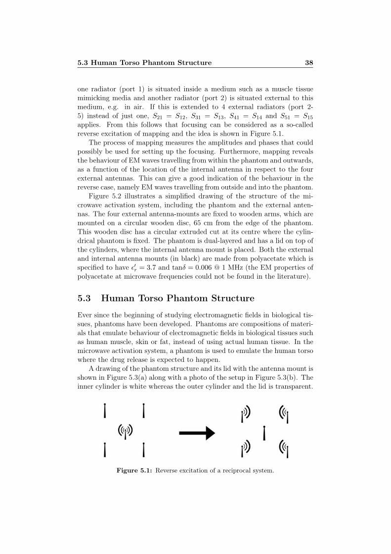
5.3 Human Torso Phantom Structure 38
one radiator (port 1) is situated inside a medium such as a muscle tissuemimicking media and another radiator (port 2) is situated external to thismedium, e.g. in air. If this is extended to 4 external radiators (port 2-5) instead of just one, S21 = S12, S31 = S13, S41 = S14 and S51 = S15applies. From this follows that focusing can be considered as a so-calledreverse excitation of mapping and the idea is shown in Figure 5.1.
The process of mapping measures the amplitudes and phases that couldpossibly be used for setting up the focusing. Furthermore, mapping revealsthe behaviour of EM waves travelling from within the phantom and outwards,as a function of the location of the internal antenna in respect to the fourexternal antennas. This can give a good indication of the behaviour in thereverse case, namely EM waves travelling from outside and into the phantom.
Figure 5.2 illustrates a simplified drawing of the structure of the mi-crowave activation system, including the phantom and the external anten-nas. The four external antenna-mounts are fixed to wooden arms, which aremounted on a circular wooden disc, 65 cm from the edge of the phantom.This wooden disc has a circular extruded cut at its centre where the cylin-drical phantom is fixed. The phantom is dual-layered and has a lid on top ofthe cylinders, where the internal antenna mount is placed. Both the externaland internal antenna mounts (in black) are made from polyacetate which isspecified to have ε′r = 3.7 and tanδ = 0.006 @ 1 MHz (the EM properties ofpolyacetate at microwave frequencies could not be found in the literature).
5.3 Human Torso Phantom Structure
Ever since the beginning of studying electromagnetic fields in biological tis-sues, phantoms have been developed. Phantoms are compositions of materi-als that emulate behaviour of electromagnetic fields in biological tissues suchas human muscle, skin or fat, instead of using actual human tissue. In themicrowave activation system, a phantom is used to emulate the human torsowhere the drug release is expected to happen.
A drawing of the phantom structure and its lid with the antenna mount isshown in Figure 5.3(a) along with a photo of the setup in Figure 5.3(b). Theinner cylinder is white whereas the outer cylinder and the lid is transparent.
Figure 5.1: Reverse excitation of a reciprocal system.
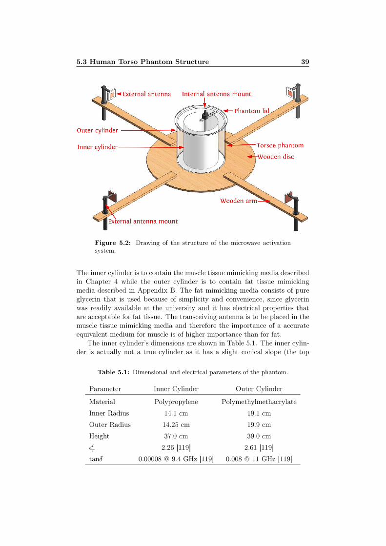
5.3 Human Torso Phantom Structure 39
Figure 5.2: Drawing of the structure of the microwave activationsystem.
The inner cylinder is to contain the muscle tissue mimicking media describedin Chapter 4 while the outer cylinder is to contain fat tissue mimickingmedia described in Appendix B. The fat mimicking media consists of pureglycerin that is used because of simplicity and convenience, since glycerinwas readily available at the university and it has electrical properties thatare acceptable for fat tissue. The transceiving antenna is to be placed in themuscle tissue mimicking media and therefore the importance of a accurateequivalent medium for muscle is of higher importance than for fat.
The inner cylinder’s dimensions are shown in Table 5.1. The inner cylin-der is actually not a true cylinder as it has a slight conical slope (the top
Table 5.1: Dimensional and electrical parameters of the phantom.
Parameter Inner Cylinder Outer Cylinder
Material Polypropylene Polymethylmethacrylate
Inner Radius 14.1 cm 19.1 cm
Outer Radius 14.25 cm 19.9 cm
Height 37.0 cm 39.0 cm
ε′r 2.26 [119] 2.61 [119]
tanδ 0.00008 @ 9.4 GHz [119] 0.008 @ 11 GHz [119]
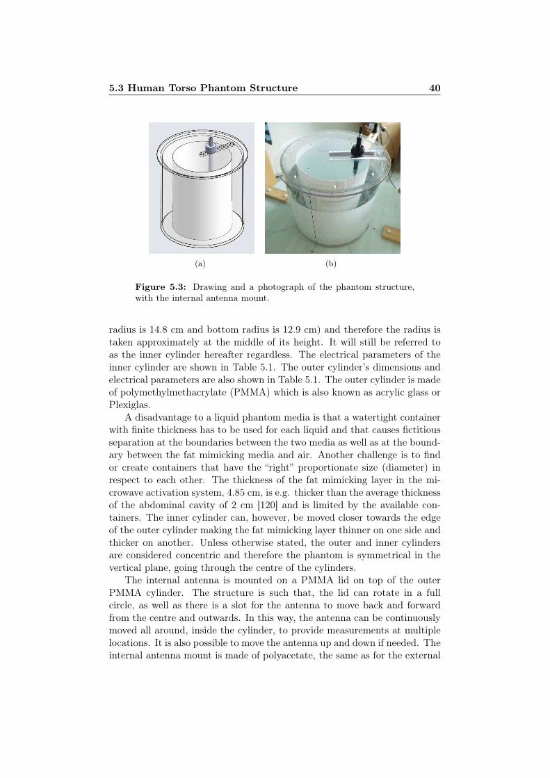
5.3 Human Torso Phantom Structure 40
(a) (b)
Figure 5.3: Drawing and a photograph of the phantom structure,with the internal antenna mount.
radius is 14.8 cm and bottom radius is 12.9 cm) and therefore the radius istaken approximately at the middle of its height. It will still be referred toas the inner cylinder hereafter regardless. The electrical parameters of theinner cylinder are shown in Table 5.1. The outer cylinder’s dimensions andelectrical parameters are also shown in Table 5.1. The outer cylinder is madeof polymethylmethacrylate (PMMA) which is also known as acrylic glass orPlexiglas.
A disadvantage to a liquid phantom media is that a watertight containerwith finite thickness has to be used for each liquid and that causes fictitiousseparation at the boundaries between the two media as well as at the bound-ary between the fat mimicking media and air. Another challenge is to findor create containers that have the “right” proportionate size (diameter) inrespect to each other. The thickness of the fat mimicking layer in the mi-crowave activation system, 4.85 cm, is e.g. thicker than the average thicknessof the abdominal cavity of 2 cm [120] and is limited by the available con-tainers. The inner cylinder can, however, be moved closer towards the edgeof the outer cylinder making the fat mimicking layer thinner on one side andthicker on another. Unless otherwise stated, the outer and inner cylindersare considered concentric and therefore the phantom is symmetrical in thevertical plane, going through the centre of the cylinders.
The internal antenna is mounted on a PMMA lid on top of the outerPMMA cylinder. The structure is such that, the lid can rotate in a fullcircle, as well as there is a slot for the antenna to move back and forwardfrom the centre and outwards. In this way, the antenna can be continuouslymoved all around, inside the cylinder, to provide measurements at multiplelocations. It is also possible to move the antenna up and down if needed. Theinternal antenna mount is made of polyacetate, the same as for the external
5.4 Continuous Wave vs. Pulsed Wave 41
antenna mounts.A doughnut shape piece of polystyrene is cut out and placed in between
the two cylinders in order to hold the inner cylinder in a semi-fixed position inrespect to the outer one. The polystyrene is placed above the fat mimickingmedia, occupying space that only occupied air before. As polystyrene is veryclose to air’s permittivity, it does not influence the phantom. The polystyreneis not shown in the figures.
A disadvantage of using glycerin as the fat layer in the dual-layered phan-tom is that, the density of glycerin is higher than the density of the muscletissue mimicking media. The inner cylinder is not completely fixed to theouter cylinder which means that inner cylinder floats, unless the volume ofthe glycerin is lowered a bit below the muscle media.
Figure 5.3 shows the phantom with a circular cross-section. The maxi-mum power transfer into the phantom at the Brewster angle, as discussedin Section 3.2.3, can be possible for (maximum) two locations on the phan-tom from every single transmitter. In a near proximity of these locations, thepower transfer will be higher than the normal incident case. A pre-destortinglens could perhaps be designed to obtain more locations of maximum powertransfer and is a task for a future research. To utilize the maximum powertransfer method in the experimental setup for focusing is complex and willnot be covered in further details in this work. Although it will not be utilizedin this work, the method was found to be interesting and I had not comeacross the combination of Brewster angle and oblique angle transmissionsinto lossy media in the literature, even though it might (probably) alreadyhave been published.
5.4 Continuous Wave vs. Pulsed Wave
When it comes to evaluating whether a continuous wave (CW) system ora pulsed wave (PW) system is best suited for microwave activation of drugrelease, several factors have to be considered such as safety, simplicity andfunctionality.
Human biophysical reactions to microwaves are mostly documented to bea thermo-physiological response. Experimental studies are in conflict whenit comes to the comparison of the biophysical response of CW comparedto PW, when the time-average radiated power is the same, or similar. In[121] and [122] e.g. no conclusive difference was found when applying PWcompared to CW. However significant decrease in arterial blood pressures inrats have been reported [123] when radiated with PW and auditory effectsuch as clicking, buzzing and hissing noises are a known response to highpeak E-field PW [124]. No conclusions can be made, currently, about therelative safety of using PW compared to CW. There seems however, to be atendency throughout the literature, that either PW and CW causes similar
5.5 System-Level Block Diagram - Mapping 42
responses in tissue or, that PW causes more negative effects than CW, ratherthan vice versa.
A pulse can be represented as a Fourier transformation including mul-tiple frequencies. As was presented in Section 4, the dielectric propertiesof biological tissues vary over frequency, making them frequency dispersive.This results in different phase velocities for waves of different frequencies ascan be seen through
vp = ω/β, (5.3)
where β is the same as presented in Equation 3.12. Lets consider two wavestravelling in a muscle tissue, one at 2.45 GHz and the other at 4.9 GHz. Thephase velocity for the 2.45 GHz would be 0.4065·108 m/s and 0.4183·108 m/sfor 4.9 GHz. Without any losses in the muscle, the phase velocities would beapproximately 1% higher than the presented values, indicating the relativeinsignificance of losses, to phase velocity in biological tissue. However, therelative permittivities of 53.6 and 50.3 at 2.45 GHz and 4.9 GHz, respectively,are responsible for the phase velocities being approximately 13-14% of thespeed of light.
For biological tissues the most dominating factor in controlling dispersionis therefore the variation in relative permittivity with frequency. The lossesin the tissues, even though they grow very fast with increasing frequency,have little influence on the dispersion. This is true as long as (σ/ωε′)2 << 1is fulfilled, which is typically the case for biological tissues at microwavefrequencies below 6 GHz (e.g. (σ/ωε′)2 = 0.06 for muscle tissue at 2.45GHz). The dispersive effects described above can cause pulses to distortwhen travelling in the human body.
Analysis of pulses done in [125] indicates that, a PW does not penetratedeeper in tissues than CW signals having frequency equal to or lower thanthe fundamental frequency of the PW since higher harmonics of the funda-mental frequency are attenuated more. The narrower the pulse is, the moreattenuation occurs [64].
When it comes to simplicity, the CW system has the advantage. Apulsed system requires e.g. a pulse generator and all the circuits need to berelatively wideband. The CW system can on the contrary, be narrowband,therefore relaxing the requirements towards components and circuit designs.
All things considered, the CW approach is selected for the microwaveactivation system for drug release.
5.5 System-Level Block Diagram - Mapping
The system block design is carried out keeping in mind that, preferably thesame equipment is to be used for both mapping and focusing, and there-fore the link budgets for both setups are realized simultaneously. Whendetermining the receiver architecture, the limitation of real components is
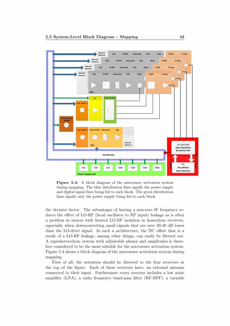
5.5 System-Level Block Diagram - Mapping 43
AttenuatorPhase Shifter VGA
Internal AntennaTX1
PA
Freq. Synth. 2
Freq. Synth. 1
NI USB-6009Data Aquisition& Control Unit
PCNI LabView
User InterfaceD
igit
al C
on
tro
l
Mea
sure
men
ts
LNA RF-BPF Attenuator VGA Mixer IF-BPF IF-AmpExternal Antenna
LNA RF-BPF Attenuator VGA Mixer IF-BPF IF-AmpExternal Antenna
LNA RF-BPF Attenuator VGA Mixer IF-BPF IF-AmpExternal Antenna
LNA RF-BPF Attenuator VGA Mixer IF-BPF IF-AmpExternal Antenna
RX1
3V3 5V0-5V0 15V0-15V0 24V012V0
Power Supply Unit
Distribution
Power Divider
OCTX Refence10 MHz
Figure 5.4: A block diagram of the microwave activation systemduring mapping. The blue distribution lines signify the power supplyand digital signal lines being fed to each block. The green distributionlines signify only the power supply being fed to each block.
the decisive factor. The advantages of having a non-zero IF frequency re-duces the effect of LO-RF (local oscillator to RF input) leakage as is oftena problem in mixers with limited LO-RF isolation in homodyne receivers,especially when downconverting small signals that are over 30-40 dB lowerthan the LO-drive signal. In such a architecture, the DC offset that is aresult of a LO-RF leakage, among other things, can easily be filtered out.A superheterodyne system with adjustable phases and amplitudes is there-fore considered to be the most suitable for the microwave activation system.Figure 5.4 shows a block diagram of the microwave activation system duringmapping.
First of all, the attention should be directed to the four receivers atthe top of the figure. Each of these receivers have, an external antennaconnected to their input. Furthermore every receiver includes a low noiseamplifier (LNA), a radio frequency band-pass filter (RF-BPF), a variable
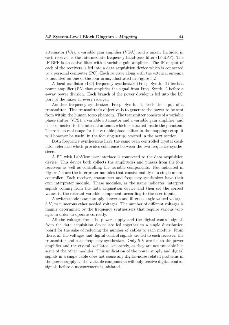
5.5 System-Level Block Diagram - Mapping 44
attenuator (VA), a variable gain amplifier (VGA), and a mixer. Included ineach receiver is the intermediate frequency band-pass filter (IF-BPF). TheIF-BPF is an active filter with a variable gain amplifier. The IF output ofeach of the receivers is fed into a data acquisition device which is connectedto a personal computer (PC). Each receiver along with the external antennais mounted on one of the four arms, illustrated in Figure 5.2
A local oscillator (LO) frequency synthesizer (Freq. Synth. 2) feeds apower amplifier (PA) that amplifies the signal from Freq. Synth. 2 before a4-way power division. Each branch of the power divider is fed into the LOport of the mixer in every receiver.
Another frequency synthesizer, Freq. Synth. 1, feeds the input of atransmitter. This transmitter’s objective is to generate the power to be sentfrom within the human torso phantom. The transmitter consists of a variablephase shifter (VPS), a variable attenuator and a variable gain amplifier, andit is connected to the internal antenna which is situated inside the phantom.There is no real usage for the variable phase shifter in the mapping setup, itwill however be useful in the focusing setup, covered in the next section.
Both frequency synthesizers have the same oven controlled crystal oscil-lator reference which provides coherence between the two frequency synthe-sizers.
A PC with LabView user interface is connected to the data acquisitiondevice. This device both collects the amplitudes and phases from the fourreceivers as well as controlling the variable components. Not indicated inFigure 5.4 are the interpreter modules that consist mainly of a single micro-controller. Each receiver, transmitter and frequency synthesizer have theirown interpreter module. These modules, as the name indicates, interpretsignals coming from the data acquisition device and then set the correctvalues to the relevant variable component, according to the user inputs.
A switch-mode power supply converts and filters a single valued voltage,5 V, to numerous other needed voltages. The number of different voltages ismainly determined by the frequency synthesizers that require various volt-ages in order to operate correctly.
All the voltages from the power supply and the digital control signalsfrom the data acquisition device are fed together to a single distributionboard for the sake of reducing the number of cables to each module. Fromthere, all the voltages and digital control signals are fed to each receiver, thetransmitter and each frequency synthesizer. Only 5 V are fed to the poweramplifier and the crystal oscillator, separately, as they are not tuneable likesome of the other modules. This unification of the power supply and digitalsignals in a single cable does not cause any digital-noise related problems inthe power supply as the variable components will only receive digital controlsignals before a measurement is initiated.
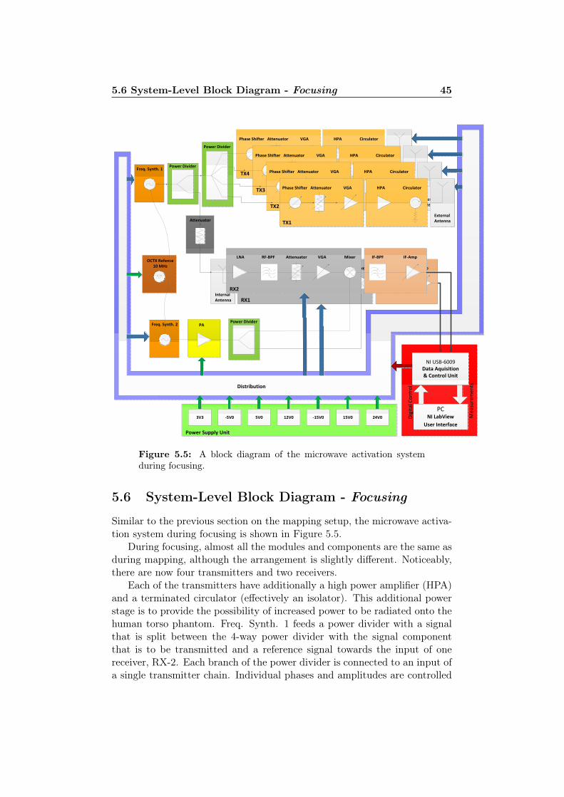
5.6 System-Level Block Diagram - Focusing 45
Freq. Synth. 1
NI USB-6009Data Aquisition& Control Unit
PCNI LabView
User Interface
Dig
ital
Co
ntr
ol
Me
asu
rem
en
ts
AttenuatorPhase Shifter VGA
TX4
HPA Circulator
External Antenna
Power Divider
AttenuatorPhase Shifter VGA
TX3
HPA Circulator
External Antenna
AttenuatorPhase Shifter VGA
TX2
HPA Circulator
External Antenna
AttenuatorPhase Shifter VGA
TX1
HPA Circulator
External Antenna
Distribution
Internal Antenna
LNA RF-BPF Attenuator VGA Mixer IF-BPF IF-Amp
RX1
3V3 5V0-5V0 15V0-15V0 24V012V0
Power Supply Unit
OCTX Refence10 MHz
PA
Attenuator
Freq. Synth. 2
LNA RF-BPF Attenuator VGA Mixer IF-BPF IF-Amp
RX2
Power Divider
Power Divider
Figure 5.5: A block diagram of the microwave activation systemduring focusing.
5.6 System-Level Block Diagram - Focusing
Similar to the previous section on the mapping setup, the microwave activa-tion system during focusing is shown in Figure 5.5.
During focusing, almost all the modules and components are the same asduring mapping, although the arrangement is slightly different. Noticeably,there are now four transmitters and two receivers.
Each of the transmitters have additionally a high power amplifier (HPA)and a terminated circulator (effectively an isolator). This additional powerstage is to provide the possibility of increased power to be radiated onto thehuman torso phantom. Freq. Synth. 1 feeds a power divider with a signalthat is split between the 4-way power divider with the signal componentthat is to be transmitted and a reference signal towards the input of onereceiver, RX-2. Each branch of the power divider is connected to an input ofa single transmitter chain. Individual phases and amplitudes are controlled
5.6 System-Level Block Diagram - Focusing 46
with the variable phase shifter, the variable attenuator and the variable gainamplifier in every transmitter chain. Each external antenna is connected tothe output of the circulator.
A receiver, RX-1, is connected to the internal antenna. The overall gainof the receiver and ultimately the amplitude of the received signal can beadjusted with the variable attenuator, variable gain amplifier and the IFamplifier, which also has variable gain. This is especially convenient duringmeasurements of signals of large dynamic range.
The power level of Freq. Synth. 2 is amplified in the PA before it is splitin two in a power divider and each part of the signal is fed to the mixers ofthe two receivers.
The input of the receiver, RX-2, is connected to an attenuator that at-tenuates the output from Freq. Synth. 1. This setup of having an additionalreceiver, such as RX-2, connected to the output of Freq. Synth. 1 (RF input)and Freq. Synth. 2 (LO input) provides a constant phase reference to thereceived signal of the internal antenna (RF input of RX-1). This is used inthe calibration process for the focusing.
Similarly as in the mapping setup, the power supply voltages and thedigital control signals are combined and then distributed to each transmitter,the receiver and to each frequency synthesizer. Not indicated in Figure 5.5is the power supply for each of the HPA which is kept separate due to theirhigh current consumption.
Both Freq. Synth. 1 and 2 can be used interchangeably in both setupssince they are identical. The specific naming of each synthesizer is arbitraryand is only to distinguish between the two. This is also valid for the receiversmentioned here, RX-1 and RX-2 which could just as well have been RX-3and RX-4 instead or any combination of the four manufactured.
All electronic modules and components will be covered in more detail inthe next chapter.
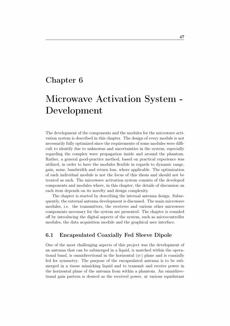
47
Chapter 6
Microwave Activation System -Development
The development of the components and the modules for the microwave acti-vation system is described in this chapter. The design of every module is notnecessarily fully optimized since the requirements of some modules were diffi-cult to identify due to unknowns and uncertainties in the system, especiallyregarding the complex wave propagation inside and around the phantom.Rather, a general good-practice method, based on practical experience wasutilized, in order to have the modules flexible in regards to dynamic range,gain, noise, bandwidth and return loss, where applicable. The optimizationof each individual module is not the focus of this thesis and should not betreated as such. The microwave activation system consists of the developedcomponents and modules where, in this chapter, the details of discussion oneach item depends on its novelty and design complexity.
The chapter is started by describing the internal antenna design. Subse-quently, the external antenna development is discussed. The main microwavemodules, i.e. the transmitters, the receivers and various other microwavecomponents necessary for the system are presented. The chapter is roundedoff by introducing the digital aspects of the system, such as microcontrollermodules, the data acquisition module and the graphical user interface.
6.1 Encapsulated Coaxially Fed Sleeve Dipole
One of the most challenging aspects of this project was the development ofan antenna that can be submerged in a liquid, is matched within the opera-tional band, is omnidirectional in the horizontal (φ-) plane and is coaxiallyfed for symmetry. The purpose of the encapsulated antenna is to be sub-merged in a tissue mimicking liquid and to transmit and receive power inthe horizontal plane of the antenna from within a phantom. An omnidirec-tional gain pattern is desired as the received power, at various equidistant
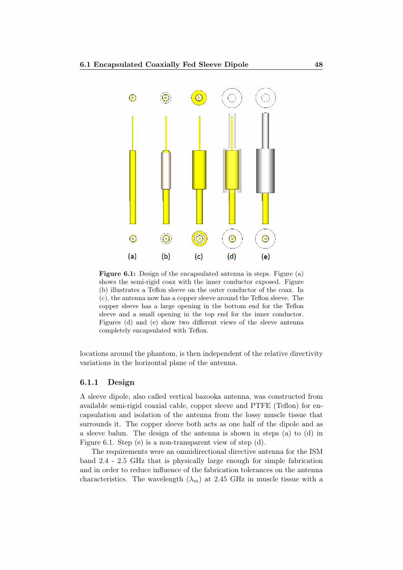
6.1 Encapsulated Coaxially Fed Sleeve Dipole 48
Figure 6.1: Design of the encapsulated antenna in steps. Figure (a)shows the semi-rigid coax with the inner conductor exposed. Figure(b) illustrates a Teflon sleeve on the outer conductor of the coax. In(c), the antenna now has a copper sleeve around the Teflon sleeve. Thecopper sleeve has a large opening in the bottom end for the Teflonsleeve and a small opening in the top end for the inner conductor.Figures (d) and (e) show two different views of the sleeve antennacompletely encapsulated with Teflon.
locations around the phantom, is then independent of the relative directivityvariations in the horizontal plane of the antenna.
6.1.1 Design
A sleeve dipole, also called vertical bazooka antenna, was constructed fromavailable semi-rigid coaxial cable, copper sleeve and PTFE (Teflon) for en-capsulation and isolation of the antenna from the lossy muscle tissue thatsurrounds it. The copper sleeve both acts as one half of the dipole and asa sleeve balun. The design of the antenna is shown in steps (a) to (d) inFigure 6.1. Step (e) is a non-transparent view of step (d).
The requirements were an omnidirectional directive antenna for the ISMband 2.4 - 2.5 GHz that is physically large enough for simple fabricationand in order to reduce influence of the fabrication tolerances on the antennacharacteristics. The wavelength (λm) at 2.45 GHz in muscle tissue with a
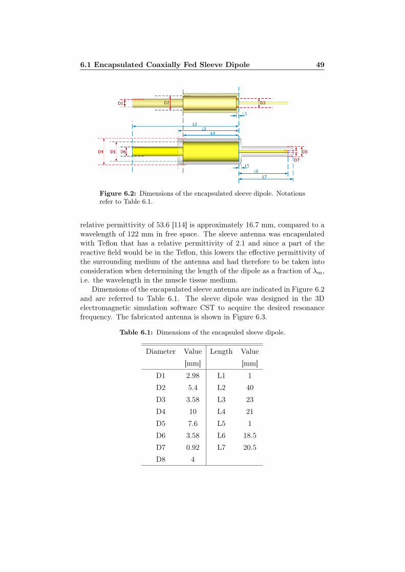
6.1 Encapsulated Coaxially Fed Sleeve Dipole 49
Figure 6.2: Dimensions of the encapsulated sleeve dipole. Notationsrefer to Table 6.1.
relative permittivity of 53.6 [114] is approximately 16.7 mm, compared to awavelength of 122 mm in free space. The sleeve antenna was encapsulatedwith Teflon that has a relative permittivity of 2.1 and since a part of thereactive field would be in the Teflon, this lowers the effective permittivity ofthe surrounding medium of the antenna and had therefore to be taken intoconsideration when determining the length of the dipole as a fraction of λm,i.e. the wavelength in the muscle tissue medium.
Dimensions of the encapsulated sleeve antenna are indicated in Figure 6.2and are referred to Table 6.1. The sleeve dipole was designed in the 3Delectromagnetic simulation software CST to acquire the desired resonancefrequency. The fabricated antenna is shown in Figure 6.3.
Table 6.1: Dimensions of the encapsuled sleeve dipole.
Diameter Value Length Value
[mm] [mm]
D1 2.98 L1 1
D2 5.4 L2 40
D3 3.58 L3 23
D4 10 L4 21
D5 7.6 L5 1
D6 3.58 L6 18.5
D7 0.92 L7 20.5
D8 4
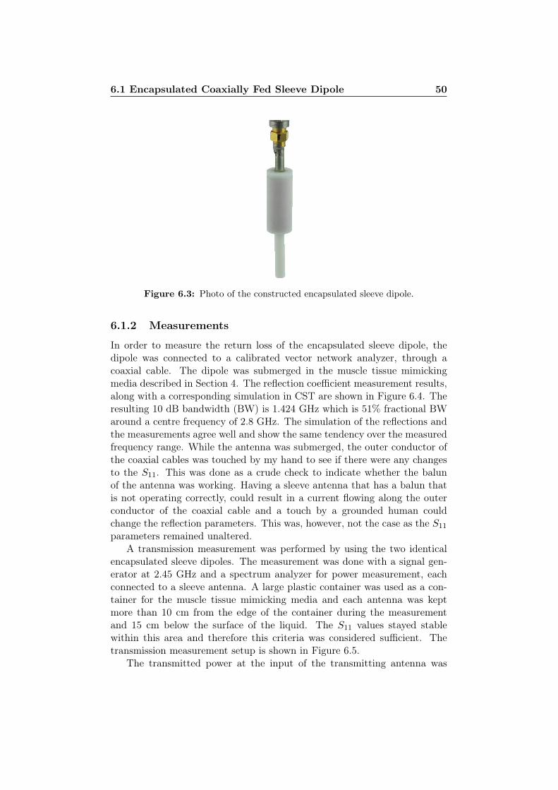
6.1 Encapsulated Coaxially Fed Sleeve Dipole 50
Figure 6.3: Photo of the constructed encapsulated sleeve dipole.
6.1.2 Measurements
In order to measure the return loss of the encapsulated sleeve dipole, thedipole was connected to a calibrated vector network analyzer, through acoaxial cable. The dipole was submerged in the muscle tissue mimickingmedia described in Section 4. The reflection coefficient measurement results,along with a corresponding simulation in CST are shown in Figure 6.4. Theresulting 10 dB bandwidth (BW) is 1.424 GHz which is 51% fractional BWaround a centre frequency of 2.8 GHz. The simulation of the reflections andthe measurements agree well and show the same tendency over the measuredfrequency range. While the antenna was submerged, the outer conductor ofthe coaxial cables was touched by my hand to see if there were any changesto the S11. This was done as a crude check to indicate whether the balunof the antenna was working. Having a sleeve antenna that has a balun thatis not operating correctly, could result in a current flowing along the outerconductor of the coaxial cable and a touch by a grounded human couldchange the reflection parameters. This was, however, not the case as the S11parameters remained unaltered.
A transmission measurement was performed by using the two identicalencapsulated sleeve dipoles. The measurement was done with a signal gen-erator at 2.45 GHz and a spectrum analyzer for power measurement, eachconnected to a sleeve antenna. A large plastic container was used as a con-tainer for the muscle tissue mimicking media and each antenna was keptmore than 10 cm from the edge of the container during the measurementand 15 cm below the surface of the liquid. The S11 values stayed stablewithin this area and therefore this criteria was considered sufficient. Thetransmission measurement setup is shown in Figure 6.5.
The transmitted power at the input of the transmitting antenna was
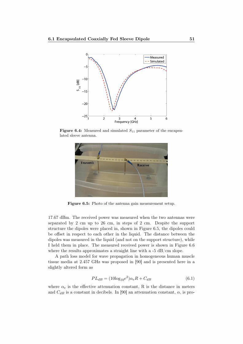
6.1 Encapsulated Coaxially Fed Sleeve Dipole 51
Figure 6.4: Measured and simulated S11 parameter of the encapsu-lated sleeve antenna.
Figure 6.5: Photo of the antenna gain measurement setup.
17.67 dBm. The received power was measured when the two antennas wereseparated by 2 cm up to 26 cm, in steps of 2 cm. Despite the supportstructure the dipoles were placed in, shown in Figure 6.5, the dipoles couldbe offset in respect to each other in the liquid. The distance between thedipoles was measured in the liquid (and not on the support structure), whileI held them in place. The measured received power is shown in Figure 6.6where the results approximates a straight line with a -5 dB/cm slope.
A path loss model for wave propagation in homogeneous human muscletissue media at 2.457 GHz was proposed in [90] and is presented here in aslightly altered form as
PLdB = (10log10e2)αeR+ CdB (6.1)
where αe is the effective attenuation constant, R is the distance in metersand CdB is a constant in decibels. In [90] an attenuation constant, α, is pro-
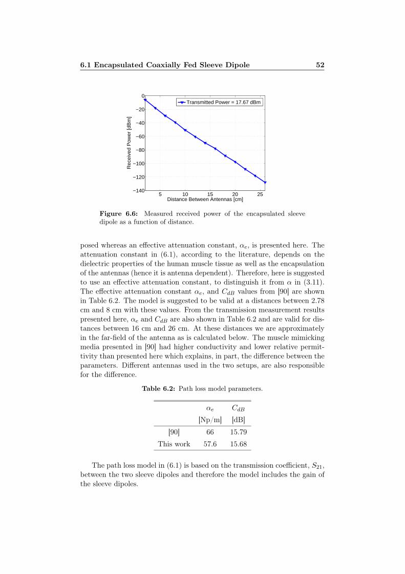
6.1 Encapsulated Coaxially Fed Sleeve Dipole 52
5 10 15 20 25−140
−120
−100
−80
−60
−40
−20
0
Distance Between Antennas [cm]
Rec
eive
d P
ower
[dB
m]
Transmitted Power = 17.67 dBm
Figure 6.6: Measured received power of the encapsulated sleevedipole as a function of distance.
posed whereas an effective attenuation constant, αe, is presented here. Theattenuation constant in (6.1), according to the literature, depends on thedielectric properties of the human muscle tissue as well as the encapsulationof the antennas (hence it is antenna dependent). Therefore, here is suggestedto use an effective attenuation constant, to distinguish it from α in (3.11).The effective attenuation constant αe, and CdB values from [90] are shownin Table 6.2. The model is suggested to be valid at a distances between 2.78cm and 8 cm with these values. From the transmission measurement resultspresented here, αe and CdB are also shown in Table 6.2 and are valid for dis-tances between 16 cm and 26 cm. At these distances we are approximatelyin the far-field of the antenna as is calculated below. The muscle mimickingmedia presented in [90] had higher conductivity and lower relative permit-tivity than presented here which explains, in part, the difference between theparameters. Different antennas used in the two setups, are also responsiblefor the difference.
Table 6.2: Path loss model parameters.
αe CdB
[Np/m] [dB]
[90] 66 15.79
This work 57.6 15.68
The path loss model in (6.1) is based on the transmission coefficient, S21,between the two sleeve dipoles and therefore the model includes the gain ofthe sleeve dipoles.
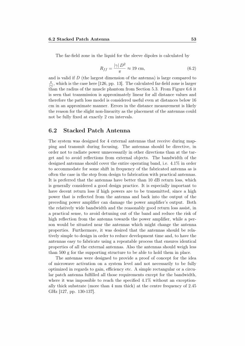
6.2 Stacked Patch Antenna 53
The far-field zone in the liquid for the sleeve dipoles is calculated by
Rff =|γ|D2
π≈ 19 cm, (6.2)
and is valid if D (the largest dimension of the antenna) is large compared toπ|γ| , which is the case here [126, pp. 13]. The calculated far-field zone is largerthan the radius of the muscle phantom from Section 5.3. From Figure 6.6 itis seen that transmission is approximately linear for all distance values andtherefore the path loss model is considered useful even at distances below 16cm in an approximate manner. Errors in the distance measurement is likelythe reason for the slight non-linearity as the placement of the antennas couldnot be fully fixed at exactly 2 cm intervals.
6.2 Stacked Patch Antenna
The system was designed for 4 external antennas that receive during map-ping and transmit during focusing. The antennas should be directive, inorder not to radiate power unnecessarily in other directions than at the tar-get and to avoid reflections from external objects. The bandwidth of thedesigned antennas should cover the entire operating band, i.e. 4.1% in orderto accommodate for some shift in frequency of the fabricated antenna as isoften the case in the step from design to fabrication with practical antennas.It is preferred that the antennas have better than 10 dB return loss, whichis generally considered a good design practice. It is especially important tohave decent return loss if high powers are to be transmitted, since a highpower that is reflected from the antenna and back into the output of thepreceding power amplifier can damage the power amplifier’s output. Boththe relatively wide bandwidth and the reasonably good return loss assist, ina practical sense, to avoid detuning out of the band and reduce the risk ofhigh reflection from the antenna towards the power amplifier, while a per-son would be situated near the antennas which might change the antennaproperties. Furthermore, it was desired that the antennas should be rela-tively simple to design in order to reduce development time and, to have theantennas easy to fabricate using a repeatable process that ensures identicalproperties of all the external antennas. Also the antennas should weigh lessthan 500 g for the supporting structure to be able to hold them in place.
The antennas were designed to provide a proof of concept for the ideaof microwave activation on a system level and not necessarily to be fullyoptimized in regards to gain, efficiency etc. A simple rectangular or a circu-lar patch antenna fulfilled all those requirements except for the bandwidth,where it was impossible to reach the specified 4.1% without an exception-ally thick substrate (more than 4 mm thick) at the centre frequency of 2.45GHz [127, pp. 130-137].
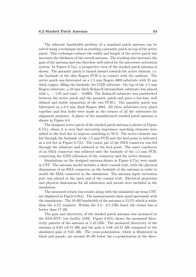
6.2 Stacked Patch Antenna 54
The inherent bandwidth problem of a standard patch antenna can besolved using a technique such as stacking a parasitic patch on top of the activepatch. This technique reduces the width and length of the active patch butincreases the thickness of the overall antenna. The stacking also increases thegain of the antenna and was therefore well suited for the microwave activationsystem. In Figure 6.7(a), a perspective view of the stacked patch antenna isshown. The parasitic patch is turned inward towards the active element, i.e.the backside of the thin Rogers PCB is in contact with the ambient. Theactive patch was fabricated on a 1.5 mm Rogers 4003 substrate with 35 µmthick copper, filling the backside, for GND reference. On top of the 1.5 mmRogers substrate, a 10 mm thick Rohacell intermediate substrate was placedwith εr = 1.05 and tanδ = 0.0002. The Rohacell substrate was sandwichedbetween the active patch and the parasitic patch and gives a low-loss, welldefined and stable separation of the two PCB’s. The parasitic patch wasfabricated on a 0.2 mm thick Rogers 4003. All three substrates were gluedtogether and four holes were made in the corners of all the substrates foralignment purposes. A photo of the manufactured stacked patch antenna isshown in Figure 6.8.
The designed active patch of the stacked patch antenna is shown in Figure6.7(b), where it is seen that microstrip impedance matching elements wereadded to the feed line to improve matching to 50 Ω. The active element wasfed through the backside of the 1.5 mm PCB and the feed point is indicatedas a red dot in Figure 6.7(b). The centre pin of the SMA connector was fedthrough the substrate and soldered at the feed point. The outer conductorof an SMA connector was soldered onto the backside of the 1.5 mm PCB,connecting the GND references of the connector and the active element.
Simulations on the designed antenna shown in Figure 6.7(a) were madein CST. The antenna model includes a short coaxial stub, with the physicaldimensions of an SMA connector on the backside of the antenna in order tomodel the SMA connector in the simulation. The antenna input excitationport was placed at the open end of the coaxial stub. Electrical propertiesand physical dimensions for all substrates and metals were included in thesimulation.
The measured return loss results along with the simulated one from CST,are displayed in Figure 6.9(a). The measurements show good agreement withthe simulations. The 10 dB bandwidth of the antenna is 13.5% which is widerthan the 4.1% required. Within the 2.4 - 2.5 GHz band, the return loss isbetter than 17 dB.
The gain and directivity of the stacked patch antenna was measured atthe ESA-DTU test facility [128]. Figure 6.9(b) shows the measured direc-tivity pattern of the antenna at 2.45 GHz. The measured directivity of theantenna is 8.83 ±0.15 dBi and the gain is 8.68 ±0.15 dBi compared to thesimulated gain of 8.65 dBi. The cross-polarization, which is illustrated inblack and purple, are around 40 dB below the co-polarization in the direc-
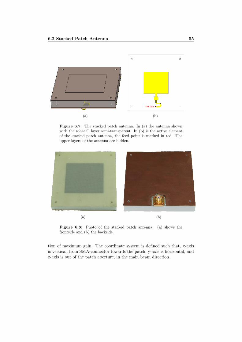
6.2 Stacked Patch Antenna 55
(a) (b)
Figure 6.7: The stacked patch antenna. In (a) the antenna shownwith the rohacell layer semi-transparent. In (b) is the active elementof the stacked patch antenna, the feed point is marked in red. Theupper layers of the antenna are hidden.
(a) (b)
Figure 6.8: Photo of the stacked patch antenna. (a) shows thefrontside and (b) the backside.
tion of maximum gain. The coordinate system is defined such that, x-axisis vertical, from SMA-connector towards the patch, y-axis is horizontal, andz-axis is out of the patch aperture, in the main beam direction.
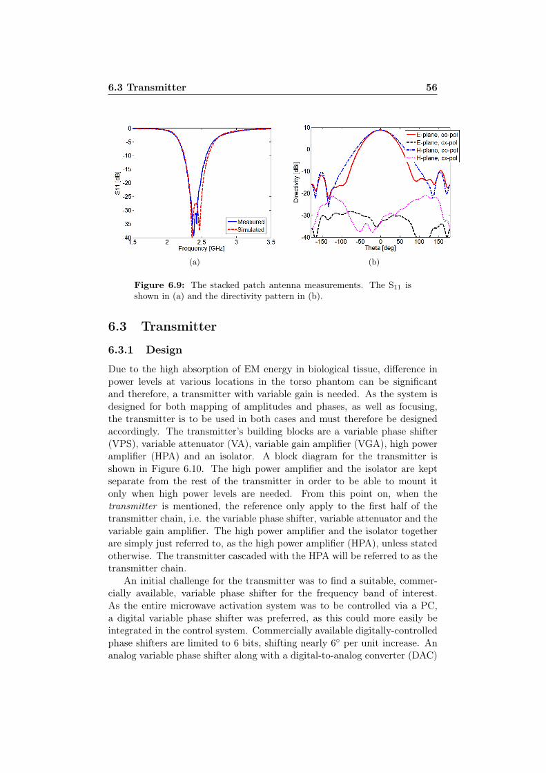
6.3 Transmitter 56
(a) (b)
Figure 6.9: The stacked patch antenna measurements. The S11 isshown in (a) and the directivity pattern in (b).
6.3 Transmitter
6.3.1 Design
Due to the high absorption of EM energy in biological tissue, difference inpower levels at various locations in the torso phantom can be significantand therefore, a transmitter with variable gain is needed. As the system isdesigned for both mapping of amplitudes and phases, as well as focusing,the transmitter is to be used in both cases and must therefore be designedaccordingly. The transmitter’s building blocks are a variable phase shifter(VPS), variable attenuator (VA), variable gain amplifier (VGA), high poweramplifier (HPA) and an isolator. A block diagram for the transmitter isshown in Figure 6.10. The high power amplifier and the isolator are keptseparate from the rest of the transmitter in order to be able to mount itonly when high power levels are needed. From this point on, when thetransmitter is mentioned, the reference only apply to the first half of thetransmitter chain, i.e. the variable phase shifter, variable attenuator and thevariable gain amplifier. The high power amplifier and the isolator togetherare simply just referred to, as the high power amplifier (HPA), unless statedotherwise. The transmitter cascaded with the HPA will be referred to as thetransmitter chain.
An initial challenge for the transmitter was to find a suitable, commer-cially available, variable phase shifter for the frequency band of interest.As the entire microwave activation system was to be controlled via a PC,a digital variable phase shifter was preferred, as this could more easily beintegrated in the control system. Commercially available digitally-controlledphase shifters are limited to 6 bits, shifting nearly 6 per unit increase. Ananalog variable phase shifter along with a digital-to-analog converter (DAC)
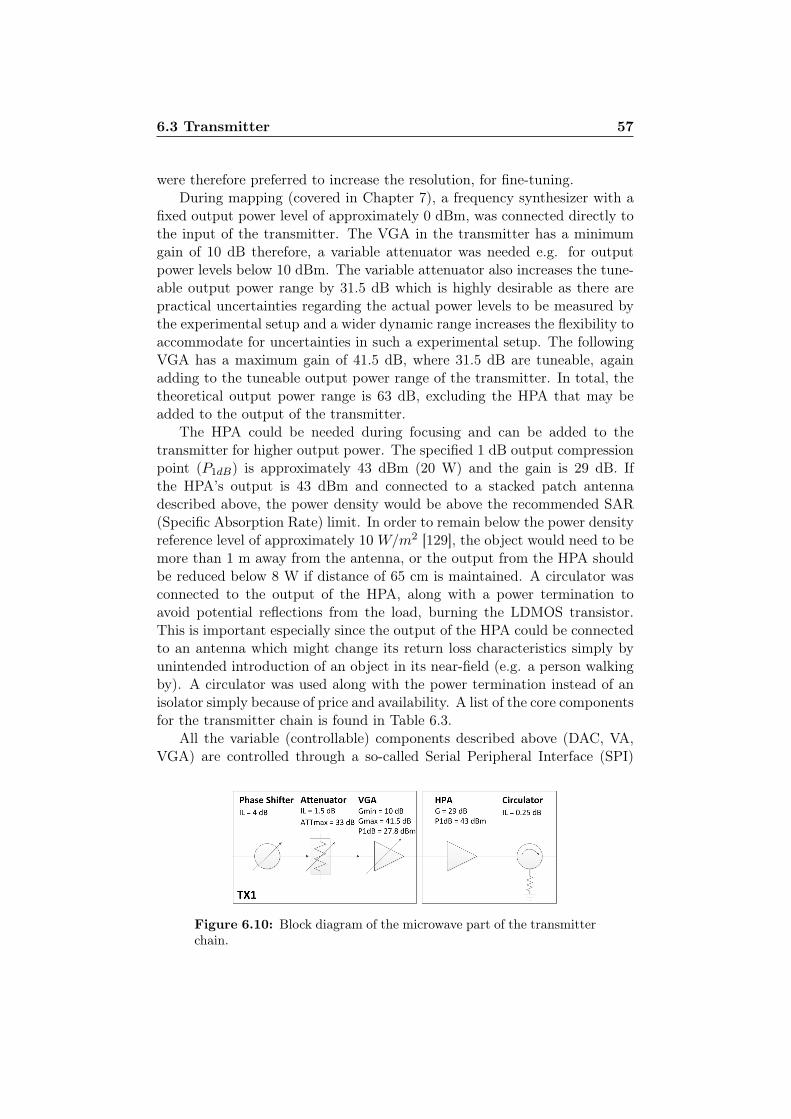
6.3 Transmitter 57
were therefore preferred to increase the resolution, for fine-tuning.During mapping (covered in Chapter 7), a frequency synthesizer with a
fixed output power level of approximately 0 dBm, was connected directly tothe input of the transmitter. The VGA in the transmitter has a minimumgain of 10 dB therefore, a variable attenuator was needed e.g. for outputpower levels below 10 dBm. The variable attenuator also increases the tune-able output power range by 31.5 dB which is highly desirable as there arepractical uncertainties regarding the actual power levels to be measured bythe experimental setup and a wider dynamic range increases the flexibility toaccommodate for uncertainties in such a experimental setup. The followingVGA has a maximum gain of 41.5 dB, where 31.5 dB are tuneable, againadding to the tuneable output power range of the transmitter. In total, thetheoretical output power range is 63 dB, excluding the HPA that may beadded to the output of the transmitter.
The HPA could be needed during focusing and can be added to thetransmitter for higher output power. The specified 1 dB output compressionpoint (P1dB) is approximately 43 dBm (20 W) and the gain is 29 dB. Ifthe HPA’s output is 43 dBm and connected to a stacked patch antennadescribed above, the power density would be above the recommended SAR(Specific Absorption Rate) limit. In order to remain below the power densityreference level of approximately 10 W/m2 [129], the object would need to bemore than 1 m away from the antenna, or the output from the HPA shouldbe reduced below 8 W if distance of 65 cm is maintained. A circulator wasconnected to the output of the HPA, along with a power termination toavoid potential reflections from the load, burning the LDMOS transistor.This is important especially since the output of the HPA could be connectedto an antenna which might change its return loss characteristics simply byunintended introduction of an object in its near-field (e.g. a person walkingby). A circulator was used along with the power termination instead of anisolator simply because of price and availability. A list of the core componentsfor the transmitter chain is found in Table 6.3.
All the variable (controllable) components described above (DAC, VA,VGA) are controlled through a so-called Serial Peripheral Interface (SPI)
Figure 6.10: Block diagram of the microwave part of the transmitterchain.
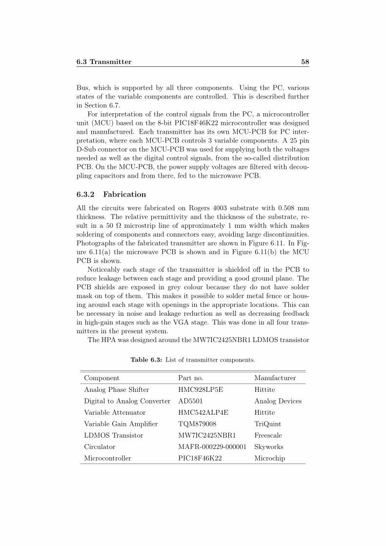
6.3 Transmitter 58
Bus, which is supported by all three components. Using the PC, variousstates of the variable components are controlled. This is described furtherin Section 6.7.
For interpretation of the control signals from the PC, a microcontrollerunit (MCU) based on the 8-bit PIC18F46K22 microcontroller was designedand manufactured. Each transmitter has its own MCU-PCB for PC inter-pretation, where each MCU-PCB controls 3 variable components. A 25 pinD-Sub connector on the MCU-PCB was used for supplying both the voltagesneeded as well as the digital control signals, from the so-called distributionPCB. On the MCU-PCB, the power supply voltages are filtered with decou-pling capacitors and from there, fed to the microwave PCB.
6.3.2 Fabrication
All the circuits were fabricated on Rogers 4003 substrate with 0.508 mmthickness. The relative permittivity and the thickness of the substrate, re-sult in a 50 Ω microstrip line of approximately 1 mm width which makessoldering of components and connectors easy, avoiding large discontinuities.Photographs of the fabricated transmitter are shown in Figure 6.11. In Fig-ure 6.11(a) the microwave PCB is shown and in Figure 6.11(b) the MCUPCB is shown.
Noticeably each stage of the transmitter is shielded off in the PCB toreduce leakage between each stage and providing a good ground plane. ThePCB shields are exposed in grey colour because they do not have soldermask on top of them. This makes it possible to solder metal fence or hous-ing around each stage with openings in the appropriate locations. This canbe necessary in noise and leakage reduction as well as decreasing feedbackin high-gain stages such as the VGA stage. This was done in all four trans-mitters in the present system.
The HPA was designed around the MW7IC2425NBR1 LDMOS transistor
Table 6.3: List of transmitter components.
Component Part no. Manufacturer
Analog Phase Shifter HMC928LP5E Hittite
Digital to Analog Converter AD5501 Analog Devices
Variable Attenuator HMC542ALP4E Hittite
Variable Gain Amplifier TQM879008 TriQuint
LDMOS Transistor MW7IC2425NBR1 Freescale
Circulator MAFR-000229-000001 Skyworks
Microcontroller PIC18F46K22 Microchip
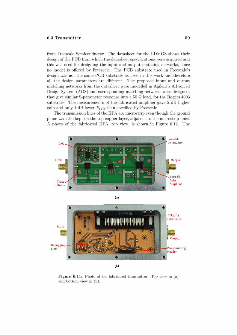
6.3 Transmitter 59
from Freescale Semiconductor. The datasheet for the LDMOS shows theirdesign of the PCB from which the datasheet specifications were acquired andthis was used for designing the input and output matching networks, sinceno model is offered by Freescale. The PCB substrate used in Freescale’sdesign was not the same PCB substrate as used in this work and thereforeall the design parameters are different. The proposed input and outputmatching networks from the datasheet were modelled in Agilent’s AdvancedDesign System (ADS) and corresponding matching networks were designed,that give similar S-parameter response into a 50 Ω load, for the Rogers 4003substrate. The measurements of the fabricated amplifier gave 2 dB highergain and only 1 dB lower P1dB than specified by Freescale.
The transmission lines of the HPA are microstrip even though the groundplane was also kept on the top copper layer, adjacent to the microstrip lines.A photo of the fabricated HPA, top view, is shown in Figure 6.12. The
Figure 6.11: Photo of the fabricated transmitter. Top view in (a)and bottom view in (b).
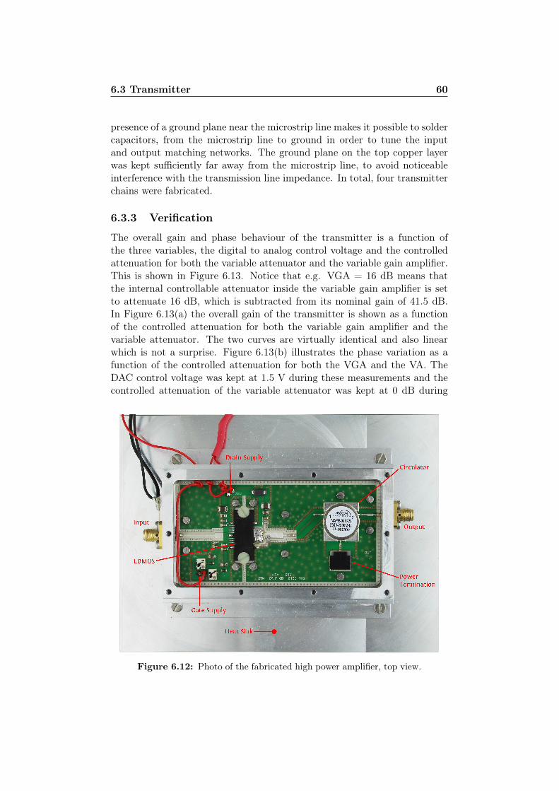
6.3 Transmitter 60
presence of a ground plane near the microstrip line makes it possible to soldercapacitors, from the microstrip line to ground in order to tune the inputand output matching networks. The ground plane on the top copper layerwas kept sufficiently far away from the microstrip line, to avoid noticeableinterference with the transmission line impedance. In total, four transmitterchains were fabricated.
6.3.3 Verification
The overall gain and phase behaviour of the transmitter is a function ofthe three variables, the digital to analog control voltage and the controlledattenuation for both the variable attenuator and the variable gain amplifier.This is shown in Figure 6.13. Notice that e.g. VGA = 16 dB means thatthe internal controllable attenuator inside the variable gain amplifier is setto attenuate 16 dB, which is subtracted from its nominal gain of 41.5 dB.In Figure 6.13(a) the overall gain of the transmitter is shown as a functionof the controlled attenuation for both the variable gain amplifier and thevariable attenuator. The two curves are virtually identical and also linearwhich is not a surprise. Figure 6.13(b) illustrates the phase variation as afunction of the controlled attenuation for both the VGA and the VA. TheDAC control voltage was kept at 1.5 V during these measurements and thecontrolled attenuation of the variable attenuator was kept at 0 dB during
Figure 6.12: Photo of the fabricated high power amplifier, top view.
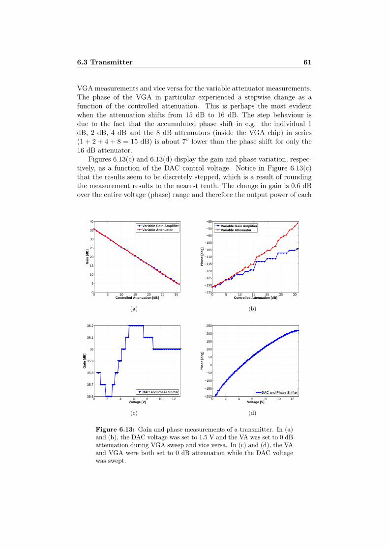
6.3 Transmitter 61
VGAmeasurements and vice versa for the variable attenuator measurements.The phase of the VGA in particular experienced a stepwise change as afunction of the controlled attenuation. This is perhaps the most evidentwhen the attenuation shifts from 15 dB to 16 dB. The step behaviour isdue to the fact that the accumulated phase shift in e.g. the individual 1dB, 2 dB, 4 dB and the 8 dB attenuators (inside the VGA chip) in series(1 + 2 + 4 + 8 = 15 dB) is about 7 lower than the phase shift for only the16 dB attenuator.
Figures 6.13(c) and 6.13(d) display the gain and phase variation, respec-tively, as a function of the DAC control voltage. Notice in Figure 6.13(c)that the results seem to be discretely stepped, which is a result of roundingthe measurement results to the nearest tenth. The change in gain is 0.6 dBover the entire voltage (phase) range and therefore the output power of each
0 5 10 15 20 25 300
5
10
15
20
25
30
35
40
Controlled Attenuation [dB]
Gai
n [
dB
]
Variable Gain AmplifierVariable Attenuator
(a)
0 5 10 15 20 25 30−135
−130
−125
−120
−115
−110
−105
−100
−95
−90
−85
Controlled Attenuation [dB]
Ph
ase
[deg
]
Variable Gain AmplifierVariable Attenuator
(b)
0 2 4 6 8 10 1235.6
35.7
35.8
35.9
36
36.1
36.2
Voltage [V]
Gai
n [
dB
]
DAC and Phase Shifter
(c)
0 2 4 6 8 10 12−200
−150
−100
−50
0
50
100
150
200
250
Voltage [V]
Ph
ase
[deg
]
DAC and Phase Shifter
(d)
Figure 6.13: Gain and phase measurements of a transmitter. In (a)and (b), the DAC voltage was set to 1.5 V and the VA was set to 0 dBattenuation during VGA sweep and vice versa. In (c) and (d), the VAand VGA were both set to 0 dB attenuation while the DAC voltagewas swept.
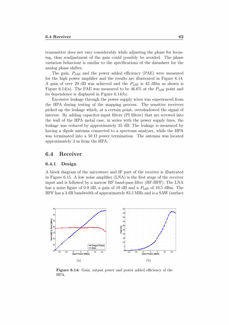
6.4 Receiver 62
transmitter does not vary considerably while adjusting the phase for focus-ing, thus readjustment of the gain could possibly be avoided. The phasevariation behaviour is similar to the specifications of the datasheet for theanalog phase shifter.
The gain, P1dB and the power added efficiency (PAE) were measuredfor the high power amplifier and the results are illustrated in Figure 6.14.A gain of over 29 dB was achieved and the P1dB is 43 dBm as shown isFigure 6.14(a). The PAE was measured to be 46.6% at the P1dB point andits dependence is displayed in Figure 6.14(b).
Excessive leakage through the power supply wires was experienced fromthe HPA during testing of the mapping process. The sensitive receiverspicked up the leakage which, at a certain point, overshadowed the signal ofinterest. By adding capacitor-input filters (PI filters) that are screwed intothe wall of the HPA metal case, in series with the power supply lines, theleakage was reduced by approximately 35 dB. The leakage is measured byhaving a dipole antenna connected to a spectrum analyzer, while the HPAwas terminated into a 50 Ω power termination. The antenna was locatedapproximately 2 m from the HPA.
6.4 Receiver
6.4.1 Design
A block diagram of the microwave and IF part of the receiver is illustratedin Figure 6.15. A low noise amplifier (LNA) is the first stage of the receiverinput and is followed by a narrow RF band-pass filter (RF-BPF). The LNAhas a noise figure of 0.9 dB, a gain of 19 dB and a P1dB of 19.5 dBm. TheBPF has a 3 dB bandwidth of approximately 83.5 MHz and is a SAW (surface
−15 −10 −5 0 5 10 1510
15
20
25
30
35
40
45
Input Power [dBm]
Gai
n [
dB
] &
Po
ut
[dB
m]
Output PowerGain
(a)
−15 −10 −5 0 5 10 150
5
10
15
20
25
30
35
40
45
50
Input Power [dBm]
PA
E [
%]
(b)
Figure 6.14: Gain, output power and power added efficiency of theHPA.
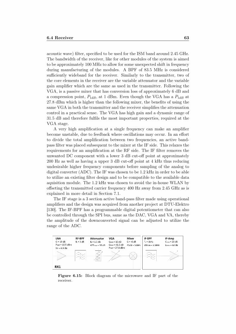
6.4 Receiver 63
acoustic wave) filter, specified to be used for the ISM band around 2.45 GHz.The bandwidth of the receiver, like for other modules of the system is aimedto be approximately 100 MHz to allow for some unexpected shift in frequencyduring manufacturing of the modules. A BPF of 83.5 MHz is consideredsufficiently wideband for the receiver. Similarly to the transmitter, two ofthe core elements in the receiver are the variable attenuator and the variablegain amplifier which are the same as used in the transmitter. Following theVGA, is a passive mixer that has conversion loss of approximately 6 dB anda compression point, P1dB, at 1 dBm. Even though the VGA has a P1dB at27.8 dBm which is higher than the following mixer, the benefits of using thesame VGA in both the transmitter and the receiver simplifies the attenuationcontrol in a practical sense. The VGA has high gain and a dynamic range of31.5 dB and therefore fulfils the most important properties, required at theVGA stage.
A very high amplification at a single frequency can make an amplifierbecome unstable, due to feedback where oscillations may occur. In an effortto divide the total amplification between two frequencies, an active band-pass filter was placed subsequent to the mixer at the IF side. This relaxes therequirements for an amplification at the RF side. The IF filter removes theunwanted DC component with a lower 3 dB cut-off point at approximately200 Hz as well as having a upper 3 dB cut-off point at 4 kHz thus reducingundesirable higher frequency components before sampling of the analog todigital converter (ADC). The IF was chosen to be 1.2 kHz in order to be ableto utilize an existing filter design and to be compatible to the available dataaquisition module. The 1.2 kHz was chosen to avoid the in-house WLAN byoffseting the transmitted carrier frequency 400 Hz away from 2.45 GHz as isexplained in more detail in Section 7.1.
The IF stage is a 3 section active band-pass filter made using operationalamplifiers and the design was acquired from another project at DTU-Elektro[130]. The IF-BPF has a programmable digital potentiometer that can alsobe controlled through the SPI bus, same as the DAC, VGA and VA, therebythe amplitude of the downconverted signal can be adjusted to utilize therange of the ADC.
Figure 6.15: Block diagram of the microwave and IF part of thereceiver.
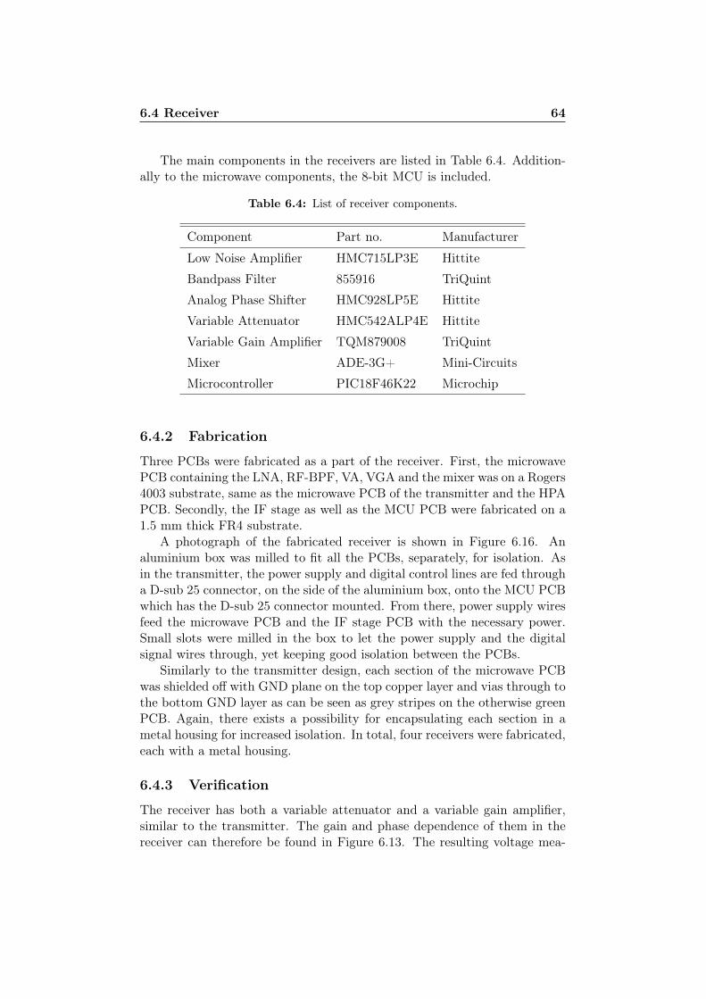
6.4 Receiver 64
The main components in the receivers are listed in Table 6.4. Addition-ally to the microwave components, the 8-bit MCU is included.
Table 6.4: List of receiver components.
Component Part no. Manufacturer
Low Noise Amplifier HMC715LP3E Hittite
Bandpass Filter 855916 TriQuint
Analog Phase Shifter HMC928LP5E Hittite
Variable Attenuator HMC542ALP4E Hittite
Variable Gain Amplifier TQM879008 TriQuint
Mixer ADE-3G+ Mini-Circuits
Microcontroller PIC18F46K22 Microchip
6.4.2 Fabrication
Three PCBs were fabricated as a part of the receiver. First, the microwavePCB containing the LNA, RF-BPF, VA, VGA and the mixer was on a Rogers4003 substrate, same as the microwave PCB of the transmitter and the HPAPCB. Secondly, the IF stage as well as the MCU PCB were fabricated on a1.5 mm thick FR4 substrate.
A photograph of the fabricated receiver is shown in Figure 6.16. Analuminium box was milled to fit all the PCBs, separately, for isolation. Asin the transmitter, the power supply and digital control lines are fed througha D-sub 25 connector, on the side of the aluminium box, onto the MCU PCBwhich has the D-sub 25 connector mounted. From there, power supply wiresfeed the microwave PCB and the IF stage PCB with the necessary power.Small slots were milled in the box to let the power supply and the digitalsignal wires through, yet keeping good isolation between the PCBs.
Similarly to the transmitter design, each section of the microwave PCBwas shielded off with GND plane on the top copper layer and vias through tothe bottom GND layer as can be seen as grey stripes on the otherwise greenPCB. Again, there exists a possibility for encapsulating each section in ametal housing for increased isolation. In total, four receivers were fabricated,each with a metal housing.
6.4.3 Verification
The receiver has both a variable attenuator and a variable gain amplifier,similar to the transmitter. The gain and phase dependence of them in thereceiver can therefore be found in Figure 6.13. The resulting voltage mea-
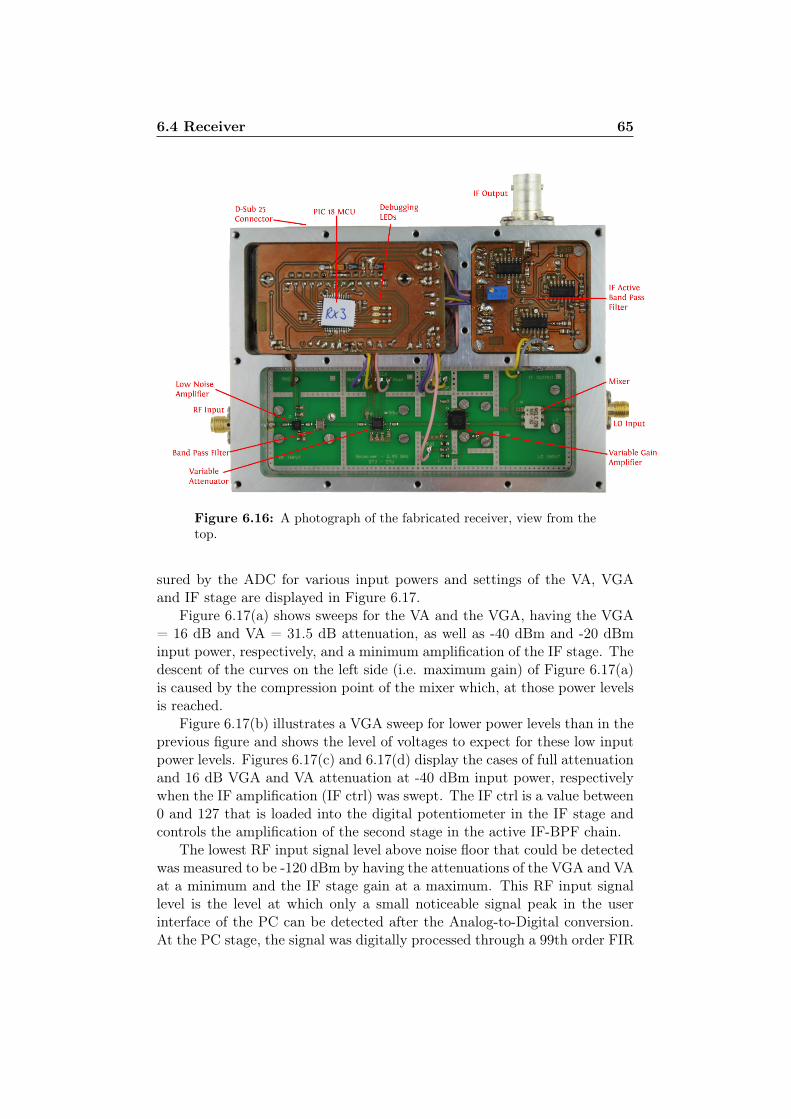
6.4 Receiver 65
Figure 6.16: A photograph of the fabricated receiver, view from thetop.
sured by the ADC for various input powers and settings of the VA, VGAand IF stage are displayed in Figure 6.17.
Figure 6.17(a) shows sweeps for the VA and the VGA, having the VGA= 16 dB and VA = 31.5 dB attenuation, as well as -40 dBm and -20 dBminput power, respectively, and a minimum amplification of the IF stage. Thedescent of the curves on the left side (i.e. maximum gain) of Figure 6.17(a)is caused by the compression point of the mixer which, at those power levelsis reached.
Figure 6.17(b) illustrates a VGA sweep for lower power levels than in theprevious figure and shows the level of voltages to expect for these low inputpower levels. Figures 6.17(c) and 6.17(d) display the cases of full attenuationand 16 dB VGA and VA attenuation at -40 dBm input power, respectivelywhen the IF amplification (IF ctrl) was swept. The IF ctrl is a value between0 and 127 that is loaded into the digital potentiometer in the IF stage andcontrols the amplification of the second stage in the active IF-BPF chain.
The lowest RF input signal level above noise floor that could be detectedwas measured to be -120 dBm by having the attenuations of the VGA and VAat a minimum and the IF stage gain at a maximum. This RF input signallevel is the level at which only a small noticeable signal peak in the userinterface of the PC can be detected after the Analog-to-Digital conversion.At the PC stage, the signal was digitally processed through a 99th order FIR
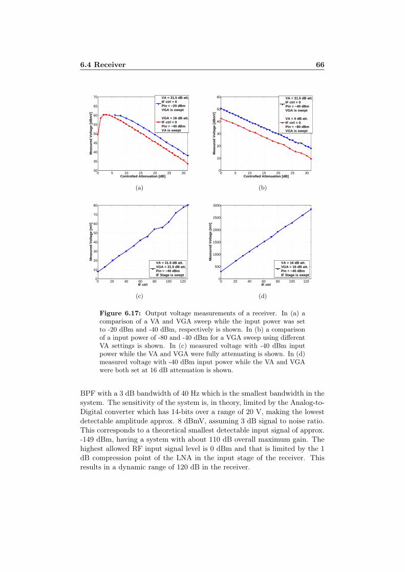
6.4 Receiver 66
0 5 10 15 20 25 3030
35
40
45
50
55
60
65
70
Controlled Attenuation [dB]
Mea
sure
d V
olta
ge [d
Bm
V]
VA = 31.5 dB att.IF ctrl = 0Pin = −20 dBmVGA is swept
VGA = 16 dB att.IF ctrl = 0Pin = −40 dBmVA is swept
(a)
0 5 10 15 20 25 300
10
20
30
40
50
60
Controlled Attenuation [dB]
Mea
sure
d V
olta
ge [d
Bm
V]
VA = 31.5 dB att.IF ctrl = 0Pin = −40 dBmVGA is swept
VA = 0 dB att.IF ctrl = 0Pin = −80 dBmVGA is swept
(b)
0 20 40 60 80 100 1200
10
20
30
40
50
60
70
80
IF ctrl
Mea
sure
d V
olta
ge [m
V]
VA = 31.5 dB att.VGA = 31.5 dB att.Pin = −40 dBmIF Stage is swept
(c)
0 20 40 60 80 100 1200
500
1000
1500
2000
2500
3000
IF ctrl
Mea
sure
d V
olta
ge [m
V]
VA = 16 dB att.VGA = 16 dB att.Pin = −40 dBmIF Stage is swept
(d)
Figure 6.17: Output voltage measurements of a receiver. In (a) acomparison of a VA and VGA sweep while the input power was setto -20 dBm and -40 dBm, respectively is shown. In (b) a comparisonof a input power of -80 and -40 dBm for a VGA sweep using differentVA settings is shown. In (c) measured voltage with -40 dBm inputpower while the VA and VGA were fully attenuating is shown. In (d)measured voltage with -40 dBm input power while the VA and VGAwere both set at 16 dB attenuation is shown.
BPF with a 3 dB bandwidth of 40 Hz which is the smallest bandwidth in thesystem. The sensitivity of the system is, in theory, limited by the Analog-to-Digital converter which has 14-bits over a range of 20 V, making the lowestdetectable amplitude approx. 8 dBmV, assuming 3 dB signal to noise ratio.This corresponds to a theoretical smallest detectable input signal of approx.-149 dBm, having a system with about 110 dB overall maximum gain. Thehighest allowed RF input signal level is 0 dBm and that is limited by the 1dB compression point of the LNA in the input stage of the receiver. Thisresults in a dynamic range of 120 dB in the receiver.
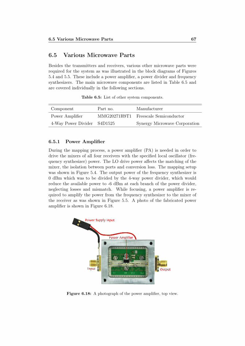
6.5 Various Microwave Parts 67
6.5 Various Microwave Parts
Besides the transmitters and receivers, various other microwave parts wererequired for the system as was illustrated in the block diagrams of Figures5.4 and 5.5. These include a power amplifier, a power divider and frequencysynthesizers. The main microwave components are listed in Table 6.5 andare covered individually in the following sections.
Table 6.5: List of other system components.
Component Part no. Manufacturer
Power Amplifier MMG20271H9T1 Freescale Semiconductor
4-Way Power Divider S4D1525 Synergy Microwave Corporation
6.5.1 Power Amplifier
During the mapping process, a power amplifier (PA) is needed in order todrive the mixers of all four receivers with the specified local oscillator (fre-quency synthesizer) power. The LO drive power affects the matching of themixer, the isolation between ports and conversion loss. The mapping setupwas shown in Figure 5.4. The output power of the frequency synthesizer is0 dBm which was to be divided by the 4-way power divider, which wouldreduce the available power to -6 dBm at each branch of the power divider,neglecting losses and mismatch. While focusing, a power amplifier is re-quired to amplify the power from the frequency synthesizer to the mixer ofthe receiver as was shown in Figure 5.5. A photo of the fabricated poweramplifier is shown in Figure 6.18.
Figure 6.18: A photograph of the power amplifier, top view.
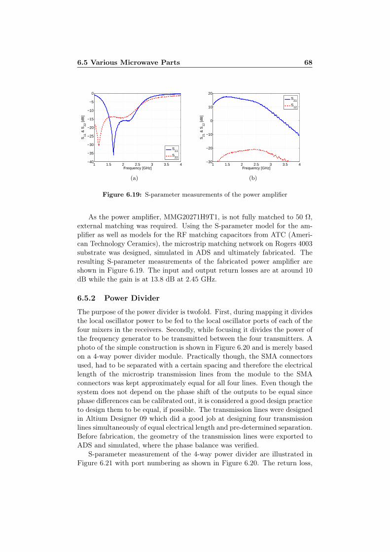
6.5 Various Microwave Parts 68
1 1.5 2 2.5 3 3.5 4−40
−35
−30
−25
−20
−15
−10
−5
0
Frequency [GHz]
S11
& S
22 [d
B]
S11
S22
(a)
1 1.5 2 2.5 3 3.5 4−30
−20
−10
0
10
20
Frequency [GHz]
S21
& S
12 [d
B]
S21
S12
(b)
Figure 6.19: S-parameter measurements of the power amplifier
As the power amplifier, MMG20271H9T1, is not fully matched to 50 Ω,external matching was required. Using the S-parameter model for the am-plifier as well as models for the RF matching capacitors from ATC (Ameri-can Technology Ceramics), the microstrip matching network on Rogers 4003substrate was designed, simulated in ADS and ultimately fabricated. Theresulting S-parameter measurements of the fabricated power amplifier areshown in Figure 6.19. The input and output return losses are at around 10dB while the gain is at 13.8 dB at 2.45 GHz.
6.5.2 Power Divider
The purpose of the power divider is twofold. First, during mapping it dividesthe local oscillator power to be fed to the local oscillator ports of each of thefour mixers in the receivers. Secondly, while focusing it divides the power ofthe frequency generator to be transmitted between the four transmitters. Aphoto of the simple construction is shown in Figure 6.20 and is merely basedon a 4-way power divider module. Practically though, the SMA connectorsused, had to be separated with a certain spacing and therefore the electricallength of the microstrip transmission lines from the module to the SMAconnectors was kept approximately equal for all four lines. Even though thesystem does not depend on the phase shift of the outputs to be equal sincephase differences can be calibrated out, it is considered a good design practiceto design them to be equal, if possible. The transmission lines were designedin Altium Designer 09 which did a good job at designing four transmissionlines simultaneously of equal electrical length and pre-determined separation.Before fabrication, the geometry of the transmission lines were exported toADS and simulated, where the phase balance was verified.
S-parameter measurement of the 4-way power divider are illustrated inFigure 6.21 with port numbering as shown in Figure 6.20. The return loss,
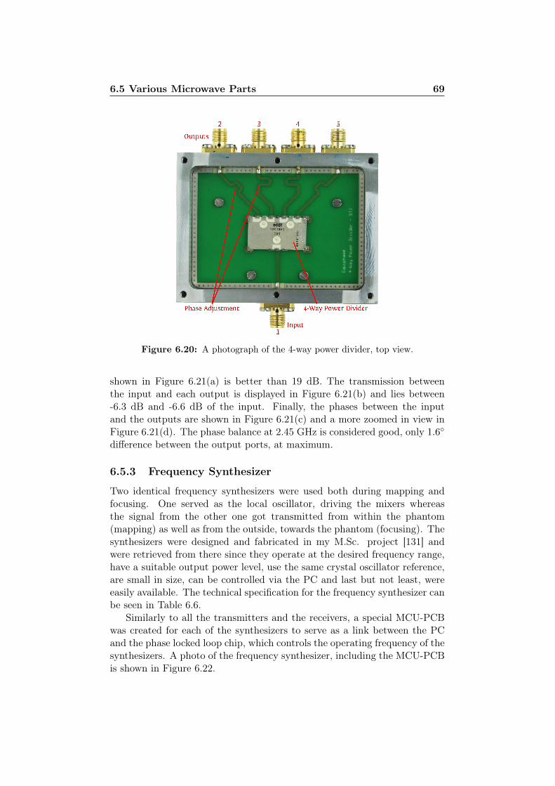
6.5 Various Microwave Parts 69
Figure 6.20: A photograph of the 4-way power divider, top view.
shown in Figure 6.21(a) is better than 19 dB. The transmission betweenthe input and each output is displayed in Figure 6.21(b) and lies between-6.3 dB and -6.6 dB of the input. Finally, the phases between the inputand the outputs are shown in Figure 6.21(c) and a more zoomed in view inFigure 6.21(d). The phase balance at 2.45 GHz is considered good, only 1.6
difference between the output ports, at maximum.
6.5.3 Frequency Synthesizer
Two identical frequency synthesizers were used both during mapping andfocusing. One served as the local oscillator, driving the mixers whereasthe signal from the other one got transmitted from within the phantom(mapping) as well as from the outside, towards the phantom (focusing). Thesynthesizers were designed and fabricated in my M.Sc. project [131] andwere retrieved from there since they operate at the desired frequency range,have a suitable output power level, use the same crystal oscillator reference,are small in size, can be controlled via the PC and last but not least, wereeasily available. The technical specification for the frequency synthesizer canbe seen in Table 6.6.
Similarly to all the transmitters and the receivers, a special MCU-PCBwas created for each of the synthesizers to serve as a link between the PCand the phase locked loop chip, which controls the operating frequency of thesynthesizers. A photo of the frequency synthesizer, including the MCU-PCBis shown in Figure 6.22.
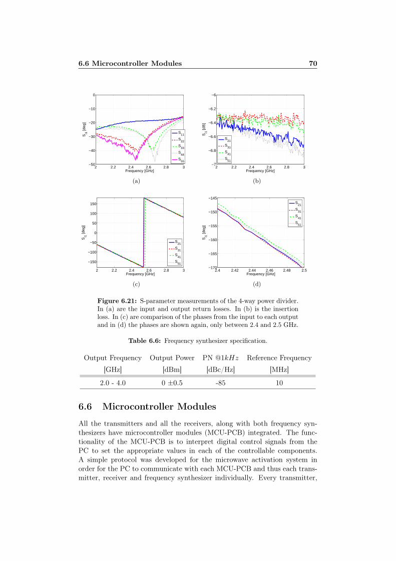
6.6 Microcontroller Modules 70
2 2.2 2.4 2.6 2.8 3−50
−40
−30
−20
−10
0
Frequency [GHz]
Si1
[deg
]
S11
S22
S33
S44
S55
(a)
2 2.2 2.4 2.6 2.8 3−7
−6.8
−6.6
−6.4
−6.2
−6
Frequency [GHz]
Si1
[dB
]
S21
S31
S41
S51
(b)
2 2.2 2.4 2.6 2.8 3
−150
−100
−50
0
50
100
150
Frequency [GHz]
Si1
[deg
]
S21
S31
S41
S51
(c)
2.4 2.42 2.44 2.46 2.48 2.5−170
−165
−160
−155
−150
−145
Frequency [GHz]
Si1
[deg
]
S21
S31
S41
S51
(d)
Figure 6.21: S-parameter measurements of the 4-way power divider.In (a) are the input and output return losses. In (b) is the insertionloss. In (c) are comparison of the phases from the input to each outputand in (d) the phases are shown again, only between 2.4 and 2.5 GHz.
Table 6.6: Frequency synthesizer specification.
Output Frequency Output Power PN @1kHz Reference Frequency
[GHz] [dBm] [dBc/Hz] [MHz]
2.0 - 4.0 0 ±0.5 -85 10
6.6 Microcontroller Modules
All the transmitters and all the receivers, along with both frequency syn-thesizers have microcontroller modules (MCU-PCB) integrated. The func-tionality of the MCU-PCB is to interpret digital control signals from thePC to set the appropriate values in each of the controllable components.A simple protocol was developed for the microwave activation system inorder for the PC to communicate with each MCU-PCB and thus each trans-mitter, receiver and frequency synthesizer individually. Every transmitter,
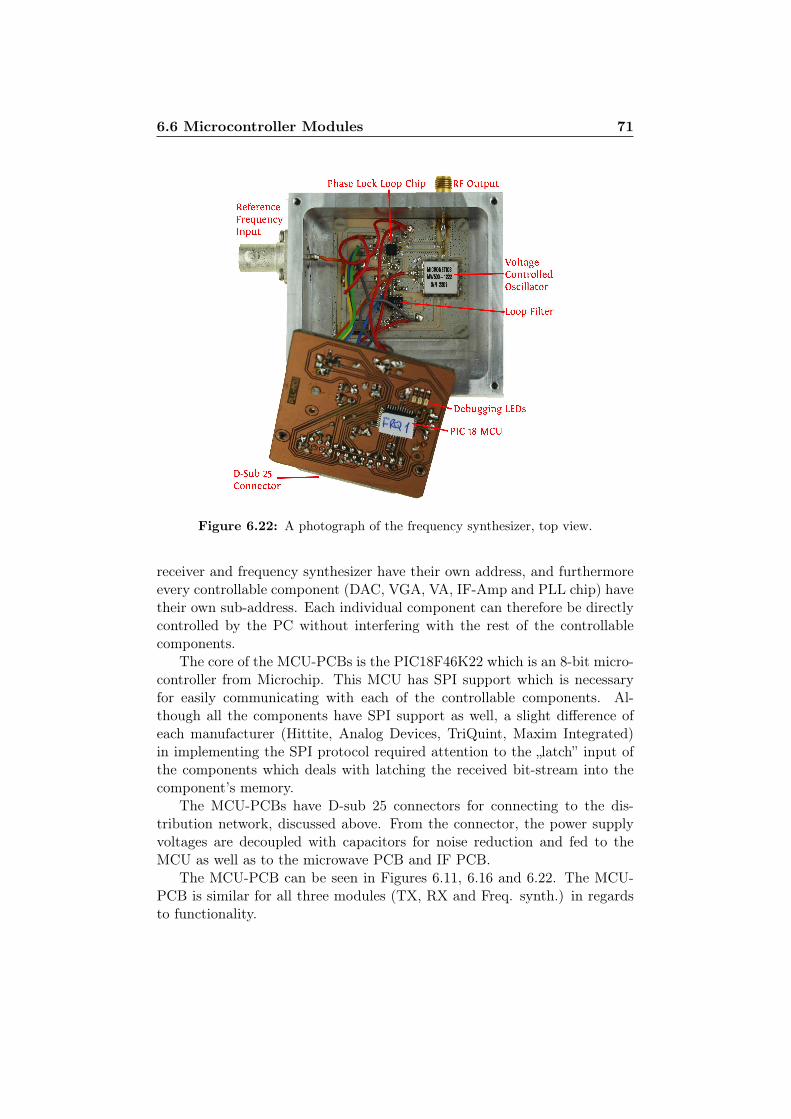
6.6 Microcontroller Modules 71
Figure 6.22: A photograph of the frequency synthesizer, top view.
receiver and frequency synthesizer have their own address, and furthermoreevery controllable component (DAC, VGA, VA, IF-Amp and PLL chip) havetheir own sub-address. Each individual component can therefore be directlycontrolled by the PC without interfering with the rest of the controllablecomponents.
The core of the MCU-PCBs is the PIC18F46K22 which is an 8-bit micro-controller from Microchip. This MCU has SPI support which is necessaryfor easily communicating with each of the controllable components. Al-though all the components have SPI support as well, a slight difference ofeach manufacturer (Hittite, Analog Devices, TriQuint, Maxim Integrated)in implementing the SPI protocol required attention to the „latch” input ofthe components which deals with latching the received bit-stream into thecomponent’s memory.
The MCU-PCBs have D-sub 25 connectors for connecting to the dis-tribution network, discussed above. From the connector, the power supplyvoltages are decoupled with capacitors for noise reduction and fed to theMCU as well as to the microwave PCB and IF PCB.
The MCU-PCB can be seen in Figures 6.11, 6.16 and 6.22. The MCU-PCB is similar for all three modules (TX, RX and Freq. synth.) in regardsto functionality.
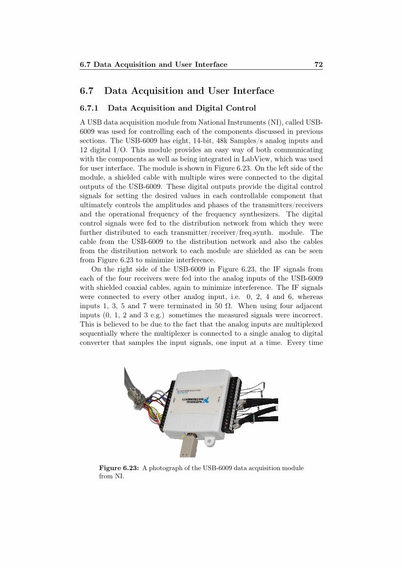
6.7 Data Acquisition and User Interface 72
6.7 Data Acquisition and User Interface
6.7.1 Data Acquisition and Digital Control
A USB data acquisition module from National Instruments (NI), called USB-6009 was used for controlling each of the components discussed in previoussections. The USB-6009 has eight, 14-bit, 48k Samples/s analog inputs and12 digital I/O. This module provides an easy way of both communicatingwith the components as well as being integrated in LabView, which was usedfor user interface. The module is shown in Figure 6.23. On the left side of themodule, a shielded cable with multiple wires were connected to the digitaloutputs of the USB-6009. These digital outputs provide the digital controlsignals for setting the desired values in each controllable component thatultimately controls the amplitudes and phases of the transmitters/receiversand the operational frequency of the frequency synthesizers. The digitalcontrol signals were fed to the distribution network from which they werefurther distributed to each transmitter/receiver/freq.synth. module. Thecable from the USB-6009 to the distribution network and also the cablesfrom the distribution network to each module are shielded as can be seenfrom Figure 6.23 to minimize interference.
On the right side of the USB-6009 in Figure 6.23, the IF signals fromeach of the four receivers were fed into the analog inputs of the USB-6009with shielded coaxial cables, again to minimize interference. The IF signalswere connected to every other analog input, i.e. 0, 2, 4 and 6, whereasinputs 1, 3, 5 and 7 were terminated in 50 Ω. When using four adjacentinputs (0, 1, 2 and 3 e.g.) sometimes the measured signals were incorrect.This is believed to be due to the fact that the analog inputs are multiplexedsequentially where the multiplexer is connected to a single analog to digitalconverter that samples the input signals, one input at a time. Every time
Figure 6.23: A photograph of the USB-6009 data acquisition modulefrom NI.
6.7 Data Acquisition and User Interface 73
an input was sampled, a capacitor in the ADC was charged up and whenmultiplexing fast between the inputs, it could cause some residual voltageon the ADC input from the previous sample. By terminating every otheranalog input this was avoided as the terminations make sure that the inputcapacitor was uncharged before next sampling.
6.7.2 User Interface
The amplitude, phase and frequency of each module were controlled from aLabView virtual instrument (VI), I developed for the microwave activationsystem. Figure 6.24 illustrates a part of the digital control user interfacein LabView. The frequency control for frequency synthesizer 1 is displayedalong with the DAC voltage control and the attenuation for TX-1 as well asthe attenuation and amplification for RX-1.
A reference frequency along with the operational frequency of each fre-quency synthesizer were typed in, in the frequency control tab where theappropriate register values were calculated and sent to the MCU-PCB ofthe frequency synthesizers. In the transmitter tab, the DAC voltage was setwhich ultimately controls the phase as illustrated in Figure 6.13(d). In boththe transmitter and receiver tabs each individual attenuator setting, 0 - 31.5dB attenuation with 0.5 dB steps were set for both the variable attenuatorand the variable gain amplifier and are represented with 16, 8, 4, 2, 1 and0.5 dB buttons. Finally, the IF amplifier was controlled with a slider in thereceiver tab.
The received IF signals are illustrated in graphs in tabs for each individ-ual receiver, RX-1 to RX-4. This includes a fast Fourier transform (FFT)of the received signals before and after software filtering for visualization ofthe frequency content of each IF signal. The amplitudes and relative phasesare displayed in the total received signal tab where the IF signals can becompared. From this tab, the automatic measurements are controlled. Ameasurement was taken every 20 seconds, which provided a pause to changethe position of the internal antenna before the next measurement. A screen-shot of few of the tabs is shown in Figure 6.25.
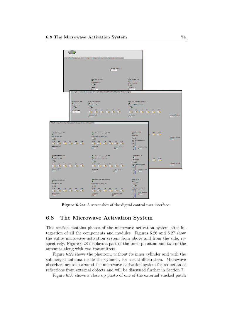
6.8 The Microwave Activation System 74
Figure 6.24: A screenshot of the digital control user interface.
6.8 The Microwave Activation System
This section contains photos of the microwave activation system after in-tegration of all the components and modules. Figures 6.26 and 6.27 showthe entire microwave activation system from above and from the side, re-spectively. Figure 6.28 displays a part of the torso phantom and two of theantennas along with two transmitters.
Figure 6.29 shows the phantom, without its inner cylinder and with thesubmerged antenna inside the cylinder, for visual illustration. Microwaveabsorbers are seen around the microwave activation system for reduction ofreflections from external objects and will be discussed further in Section 7.
Figure 6.30 shows a close up photo of one of the external stacked patch
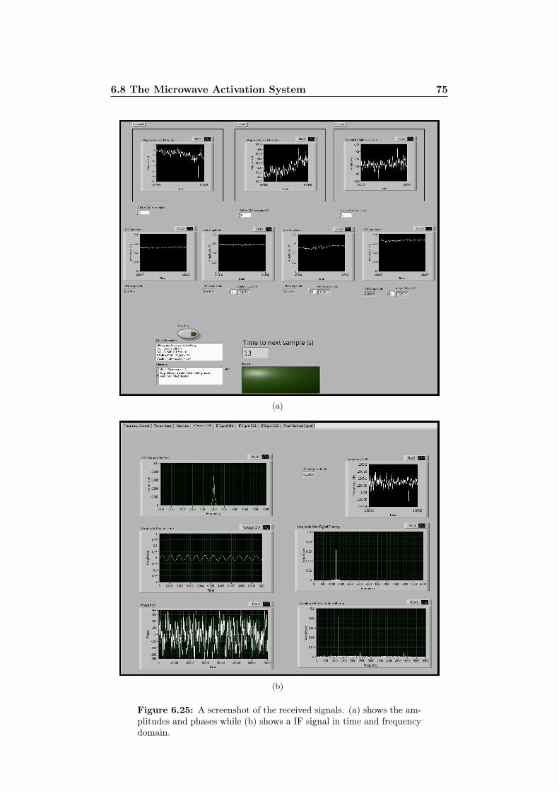
6.8 The Microwave Activation System 75
(a)
(b)
Figure 6.25: A screenshot of the received signals. (a) shows the am-plitudes and phases while (b) shows a IF signal in time and frequencydomain.
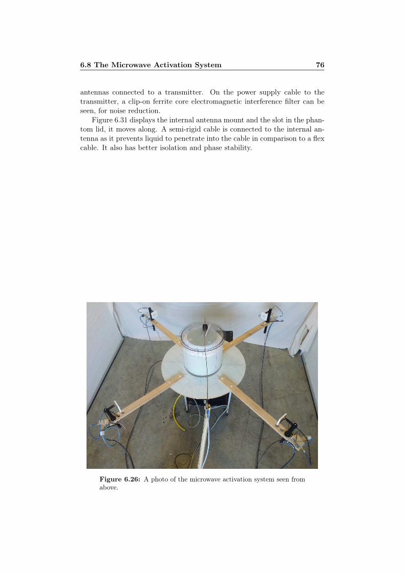
6.8 The Microwave Activation System 76
antennas connected to a transmitter. On the power supply cable to thetransmitter, a clip-on ferrite core electromagnetic interference filter can beseen, for noise reduction.
Figure 6.31 displays the internal antenna mount and the slot in the phan-tom lid, it moves along. A semi-rigid cable is connected to the internal an-tenna as it prevents liquid to penetrate into the cable in comparison to a flexcable. It also has better isolation and phase stability.
Figure 6.26: A photo of the microwave activation system seen fromabove.
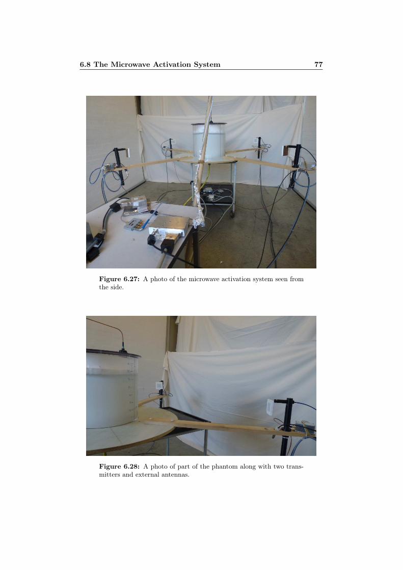
6.8 The Microwave Activation System 77
Figure 6.27: A photo of the microwave activation system seen fromthe side.
Figure 6.28: A photo of part of the phantom along with two trans-mitters and external antennas.
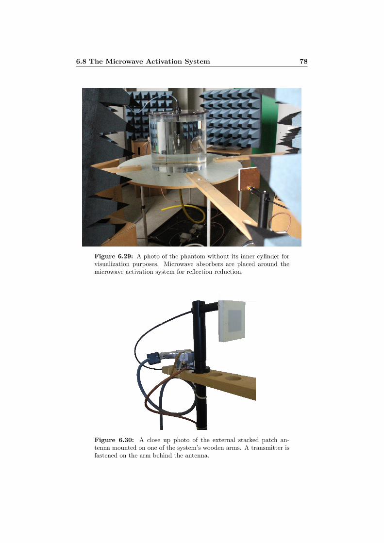
6.8 The Microwave Activation System 78
Figure 6.29: A photo of the phantom without its inner cylinder forvisualization purposes. Microwave absorbers are placed around themicrowave activation system for reflection reduction.
Figure 6.30: A close up photo of the external stacked patch an-tenna mounted on one of the system’s wooden arms. A transmitter isfastened on the arm behind the antenna.
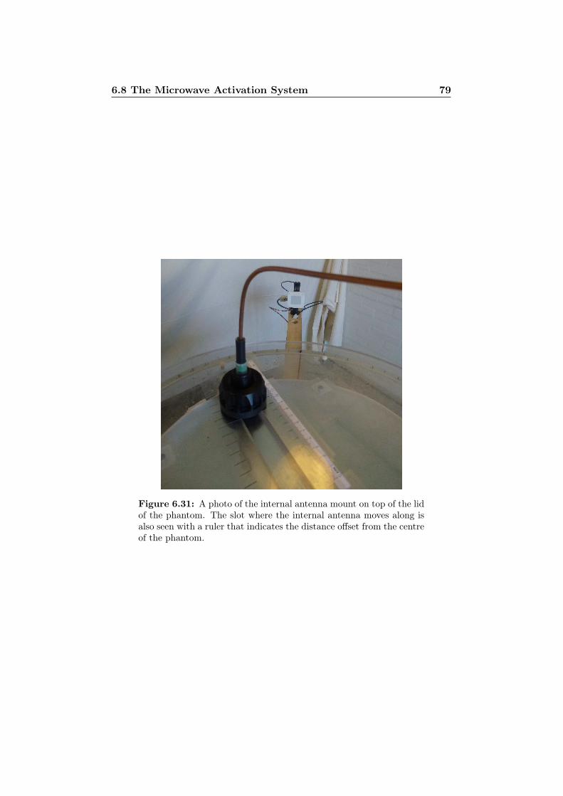
6.8 The Microwave Activation System 79
Figure 6.31: A photo of the internal antenna mount on top of the lidof the phantom. The slot where the internal antenna moves along isalso seen with a ruler that indicates the distance offset from the centreof the phantom.

80
Chapter 7
System Measurements -Mapping
In this chapter, attention is directed at a source, transmitting from within aphantom that is representing the human torso. Four receivers are distributedaround the phantom in an annular manner to measure the resulting fields.Transmission from within a cylindrically layered structure such as the hu-man torso phantom is of great interest when examining the wave behaviourinside and around a human torso. Amplitudes and phases on the outsideof the phantom will vary as the transmitting source inside the phantom ismoved around. This dependency will be mapped with measurements, basedon the experimental setup that was introduced in Section 5.5 using the man-ufactured modules presented in Chapter 6. The measurement results arecompared to simulation results and their deviations are discussed in thischapter.
7.1 Measurement Setup
In the microwave activation system where high dynamic range is required tomeasure high signal levels at one point and very low signal levels at another,the influence of reflections from external objects had to be minimized. Ife.g., the transmitted signal from within the phantom has a high power levelwhen it exits at one point of the phantom and a very low power level atanother point, external objects can in fact reflect the high level signal in away that it overshadows the low level signal. This would cause an incorrectmeasurement and distort the overall mapping. The risk of reflections fromexternal objects was reduced with the introduction of microwave absorbers.In Figure 7.1, a simple representation of the microwave activation system isillustrated along with the microwave absorbers. Eight microwave absorberswere placed in the plane of measurement, where one was placed behind eachreceiver and one between each receiver as shown in the figure. The absorbers
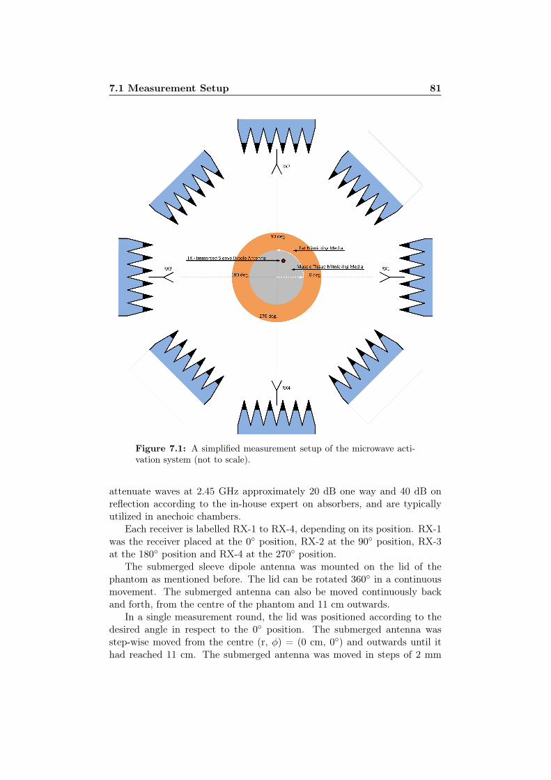
7.1 Measurement Setup 81
Figure 7.1: A simplified measurement setup of the microwave acti-vation system (not to scale).
attenuate waves at 2.45 GHz approximately 20 dB one way and 40 dB onreflection according to the in-house expert on absorbers, and are typicallyutilized in anechoic chambers.
Each receiver is labelled RX-1 to RX-4, depending on its position. RX-1was the receiver placed at the 0 position, RX-2 at the 90 position, RX-3at the 180 position and RX-4 at the 270 position.
The submerged sleeve dipole antenna was mounted on the lid of thephantom as mentioned before. The lid can be rotated 360 in a continuousmovement. The submerged antenna can also be moved continuously backand forth, from the centre of the phantom and 11 cm outwards.
In a single measurement round, the lid was positioned according to thedesired angle in respect to the 0 position. The submerged antenna wasstep-wise moved from the centre (r, φ) = (0 cm, 0) and outwards until ithad reached 11 cm. The submerged antenna was moved in steps of 2 mm
7.1 Measurement Setup 82
with a typical uncertainty of ±0.5 mm, for each measurement. The 2 mmstep were chosen as this is approximately λm/8 and was the smallest stepsize the antenna can be reliably moved in a manual manner. The submergedantenna mount was made of a plastic screw on the lid, and when displacingthe antenna, the screw was loosened, moved and then tightened again beforea new measurement was taken. Alongside the slot in the lid, where theantenna moved back and forth, there is a fixed ruler with 1 mm resolutionand on the antenna mount there is a slot, used as a reference for the internalantenna in respect to the ruler. A close-up of the antenna mount and the slotwith the ruler was shown in Figure 6.31. The displacement of the antennawas controlled manually which explains the uncertainty of typically ±0.5mm.
An automatic measurement could be started as described in Section 6.7where the computer took a measurement every 20 seconds. After each repo-sitioning of the internal antenna, I stepped behind one of the absorbers toreduce the risk of being a source of reflection and therefore disturbing themeasurements.
The frequency of synthesizer 1 was set to 2450.0004 MHz and the fre-quency of synthesizer 2 was set to 2450.0016 MHz. This provided an IF of 1.2kHz. It was found that there was a constant carrier signal at 2450.0000 MHzin the ambient, probably due to the in-house wireless network and thereforesynthesizer 1 was set at a 400 Hz offset from 2450.0000 MHz. This ambi-ent noise was measured using a spectrum analyzer with a dipole antennaconnected to its input. The carrier in question was concluded to be fromthe ambient as when the experimental setup was powered down, the carriersignal remained unchanged in both amplitude and frequency.
TX-1 was the transmitter used in the mapping process. The attenuatorsetting was set to attenuate 8 dB and the VGA has also enabled 10 dBattenuation. The receivers, RX-1 to RX-4 had attenuator settings set to 14dB and VGA set to 8 dB attenuation and finally the variable gain IF stageat a factor 23/127. This modest gain settings for the receivers preventedthe ADC to saturate when the antenna was closest to the outskirt of thephantom as well as the overall signal quality was better. The noise floor wasbelow 5 mV for these settings on the receivers and was determined from thedisplay showing the measured voltage of the IF signal in the Labview userinterface.
The height of the internal antenna was such that, the centre of the an-tenna was (vertically) in the middle from the bottom of the cylinder andthe top of the fat mimicking media. The fat mimicking media was not filledall the way to the top of the outer cylinder as mentioned before, due to theproblem with buoyancy of the inner cylinder containing the muscle tissuemimicking media. The heights of the four external antennas were adjustedso the centres of the stacked patch antennas were in the same horizontalplane as the internal antenna. The maximum gains of the external antennas
7.2 Calibration 83
were therefore in the same horizontal plane, and full advantage was taken oftheir high gain.
7.2 Calibration
When the internal antenna was placed at the centre of the phantom, thereceivers did not measure the same phase. A 0 position e.g. resulted in aslightly different phase measurements than e.g. at 135 position of the lid.
Due to variations from receiver to receiver, variation in length of SMAcoaxial cables connecting the receivers to the antennas and the local oscillatoras well as difference in distance between each external antenna to the internalantenna, the measured phases in the receivers needed calibration.
For every measurement round, at a certain position of the lid, the internalantenna was placed at the centre of the phantom. In software, the phasesare adjusted to zero. The phase control was displayed in Figure 6.25. Thiszeroing of the phases was repeated for every rotational position of the lid,immediately before measuring.
Note that when mentioning some values in degrees in the text below, ittypically refers to the phantom lid’s position and not a phase, unless statedotherwise.
7.3 Results and Discussion
Referring to Figure 7.1, a measurement round was acquired for every 10
rotational increment of the internal antenna orientation from 0 to 360.Additionally, measurements were obtained between every two receivers, i.e.at 45, 135, 225 and 315 for a symmetry comparison. The starting po-sition, defined as 0 was at the location of RX-1 as indicated in Figure7.1 for convenience. Every measurement round includes 55 measurementspoints, from 0 (centre of the phantom) and to 11 cm outwards. Since eachmeasurement point was taken discretely and the internal antenna was repo-sitioned for every measurement point, a limited number of points had to betaken. A step radially outwards of 2 mm provided a relatively dense phaseand amplitude information as every step is about 1/8 of the wavelength inthe muscle tissue mimicking media. In total, the number of discrete mea-surements points of the mapping process was 2200, which was rather timeconsuming. The number of points also had to be restricted because of longterm variation of, especially, the tissue mimicking media which evaporatedand deteriorated over time. Each of the four receivers RX-1 through RX-4,measured an amplitude and a phase. The measured phases of RX-2, RX-3and RX-4 were taken relative to the phase of RX-1, which was the reference.
A simulation model was created in COMSOL Multiphysics. A 2-D dual-layer phantom with a line current source (out of plane) that represents the
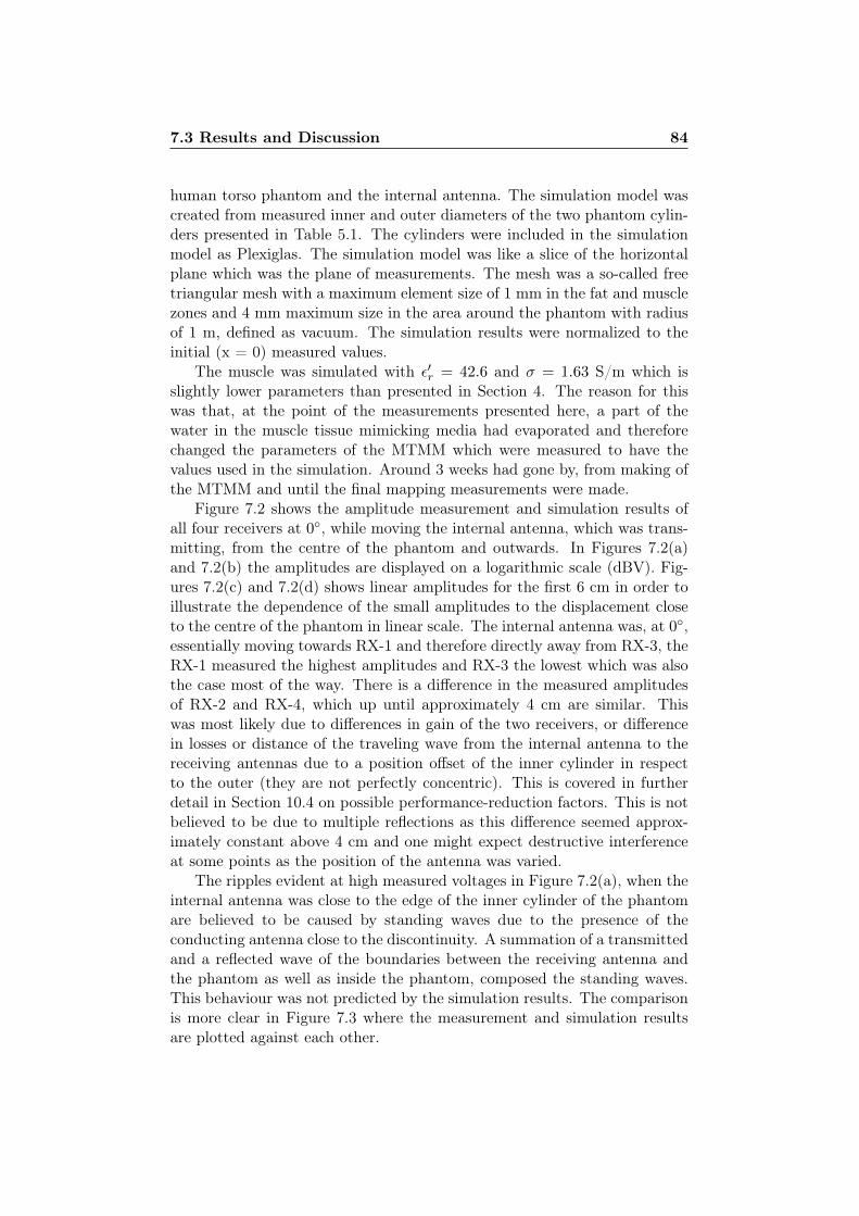
7.3 Results and Discussion 84
human torso phantom and the internal antenna. The simulation model wascreated from measured inner and outer diameters of the two phantom cylin-ders presented in Table 5.1. The cylinders were included in the simulationmodel as Plexiglas. The simulation model was like a slice of the horizontalplane which was the plane of measurements. The mesh was a so-called freetriangular mesh with a maximum element size of 1 mm in the fat and musclezones and 4 mm maximum size in the area around the phantom with radiusof 1 m, defined as vacuum. The simulation results were normalized to theinitial (x = 0) measured values.
The muscle was simulated with ε′r = 42.6 and σ = 1.63 S/m which isslightly lower parameters than presented in Section 4. The reason for thiswas that, at the point of the measurements presented here, a part of thewater in the muscle tissue mimicking media had evaporated and thereforechanged the parameters of the MTMM which were measured to have thevalues used in the simulation. Around 3 weeks had gone by, from making ofthe MTMM and until the final mapping measurements were made.
Figure 7.2 shows the amplitude measurement and simulation results ofall four receivers at 0, while moving the internal antenna, which was trans-mitting, from the centre of the phantom and outwards. In Figures 7.2(a)and 7.2(b) the amplitudes are displayed on a logarithmic scale (dBV). Fig-ures 7.2(c) and 7.2(d) shows linear amplitudes for the first 6 cm in order toillustrate the dependence of the small amplitudes to the displacement closeto the centre of the phantom in linear scale. The internal antenna was, at 0,essentially moving towards RX-1 and therefore directly away from RX-3, theRX-1 measured the highest amplitudes and RX-3 the lowest which was alsothe case most of the way. There is a difference in the measured amplitudesof RX-2 and RX-4, which up until approximately 4 cm are similar. Thiswas most likely due to differences in gain of the two receivers, or differencein losses or distance of the traveling wave from the internal antenna to thereceiving antennas due to a position offset of the inner cylinder in respectto the outer (they are not perfectly concentric). This is covered in furtherdetail in Section 10.4 on possible performance-reduction factors. This is notbelieved to be due to multiple reflections as this difference seemed approx-imately constant above 4 cm and one might expect destructive interferenceat some points as the position of the antenna was varied.
The ripples evident at high measured voltages in Figure 7.2(a), when theinternal antenna was close to the edge of the inner cylinder of the phantomare believed to be caused by standing waves due to the presence of theconducting antenna close to the discontinuity. A summation of a transmittedand a reflected wave of the boundaries between the receiving antenna andthe phantom as well as inside the phantom, composed the standing waves.This behaviour was not predicted by the simulation results. The comparisonis more clear in Figure 7.3 where the measurement and simulation resultsare plotted against each other.
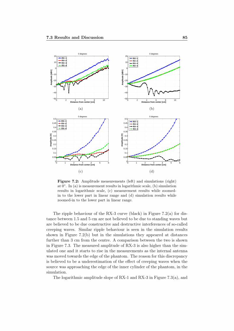
7.3 Results and Discussion 85
0 2 4 6 8 10−50
−40
−30
−20
−10
0
10
200 degrees
Distance from center [cm]
Am
plitu
de [d
BV
]
RX−1RX−2RX−3RX−4
(a)
0 2 4 6 8 10−50
−40
−30
−20
−10
0
10
200 degrees
Distance from center [cm]
Am
plitu
de [d
BV
]
RX−1RX−2RX−3RX−4
(b)
0 1 2 3 4 5 60
0.05
0.1
0.15
0.2
0.25
0.3
0.35
0.4
0.45
0.50 degrees
Distance from center [cm]
Am
plitu
de [V
]
RX−1RX−2RX−3RX−4
(c)
0 1 2 3 4 5 60
0.05
0.1
0.15
0.2
0.25
0.3
0.35
0.4
0.45
0.50 degrees
Distance from center [cm]
Am
plitu
de [V
]
RX−1RX−2RX−3RX−4
(d)
Figure 7.2: Amplitude measurements (left) and simulations (right)at 0. In (a) is measurement results in logarithmic scale, (b) simulationresults in logarithmic scale, (c) measurement results while zoomed-in to the lower part in linear range and (d) simulation results whilezoomed-in to the lower part in linear range.
The ripple behaviour of the RX-3 curve (black) in Figure 7.2(a) for dis-tance between 1.5 and 5 cm are not believed to be due to standing waves butare believed to be due constructive and destructive interferences of so-calledcreeping waves. Similar ripple behaviour is seen in the simulation resultsshown in Figure 7.2(b) but in the simulations they appeared at distancesfurther than 3 cm from the centre. A comparison between the two is shownin Figure 7.3. The measured amplitude of RX-3 is also higher than the sim-ulated one and it starts to rise in the measurements as the internal antennawas moved towards the edge of the phantom. The reason for this discrepancyis believed to be a underestimation of the effect of creeping waves when thesource was approaching the edge of the inner cylinder of the phantom, in thesimulation.
The logarithmic amplitude slope of RX-1 and RX-3 in Figure 7.3(a), and
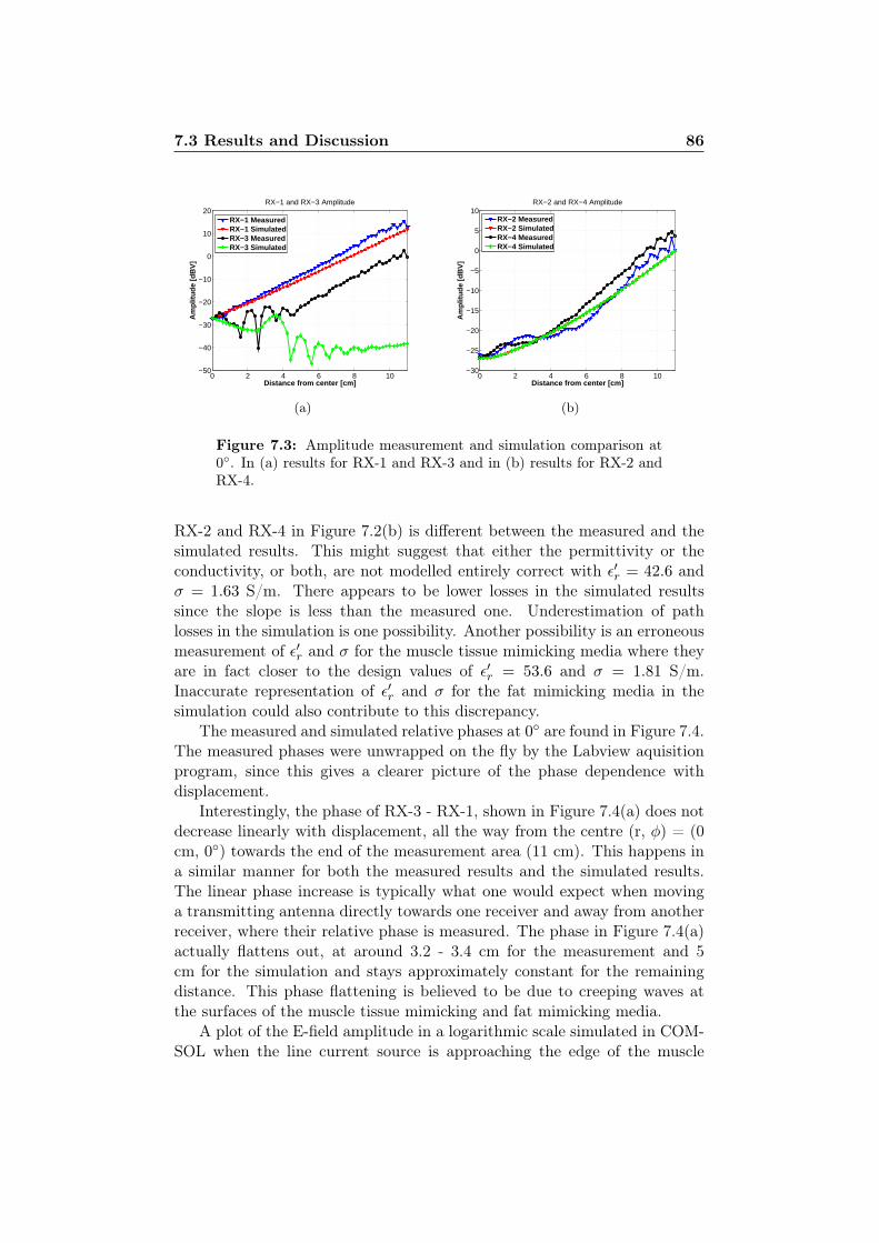
7.3 Results and Discussion 86
0 2 4 6 8 10−50
−40
−30
−20
−10
0
10
20RX−1 and RX−3 Amplitude
Distance from center [cm]
Am
plitu
de [d
BV
]
RX−1 MeasuredRX−1 SimulatedRX−3 MeasuredRX−3 Simulated
(a)
0 2 4 6 8 10−30
−25
−20
−15
−10
−5
0
5
10RX−2 and RX−4 Amplitude
Distance from center [cm]
Am
plitu
de [d
BV
]
RX−2 MeasuredRX−2 SimulatedRX−4 MeasuredRX−4 Simulated
(b)
Figure 7.3: Amplitude measurement and simulation comparison at0. In (a) results for RX-1 and RX-3 and in (b) results for RX-2 andRX-4.
RX-2 and RX-4 in Figure 7.2(b) is different between the measured and thesimulated results. This might suggest that either the permittivity or theconductivity, or both, are not modelled entirely correct with ε′r = 42.6 andσ = 1.63 S/m. There appears to be lower losses in the simulated resultssince the slope is less than the measured one. Underestimation of pathlosses in the simulation is one possibility. Another possibility is an erroneousmeasurement of ε′r and σ for the muscle tissue mimicking media where theyare in fact closer to the design values of ε′r = 53.6 and σ = 1.81 S/m.Inaccurate representation of ε′r and σ for the fat mimicking media in thesimulation could also contribute to this discrepancy.
The measured and simulated relative phases at 0 are found in Figure 7.4.The measured phases were unwrapped on the fly by the Labview aquisitionprogram, since this gives a clearer picture of the phase dependence withdisplacement.
Interestingly, the phase of RX-3 - RX-1, shown in Figure 7.4(a) does notdecrease linearly with displacement, all the way from the centre (r, φ) = (0cm, 0) towards the end of the measurement area (11 cm). This happens ina similar manner for both the measured results and the simulated results.The linear phase increase is typically what one would expect when movinga transmitting antenna directly towards one receiver and away from anotherreceiver, where their relative phase is measured. The phase in Figure 7.4(a)actually flattens out, at around 3.2 - 3.4 cm for the measurement and 5cm for the simulation and stays approximately constant for the remainingdistance. This phase flattening is believed to be due to creeping waves atthe surfaces of the muscle tissue mimicking and fat mimicking media.
A plot of the E-field amplitude in a logarithmic scale simulated in COM-SOL when the line current source is approaching the edge of the muscle
7.3 Results and Discussion 87
0 2 4 6 8 10−2000
−1800
−1600
−1400
−1200
−1000
−800
−600
−400
−200
0RX−3 − RX−1 Phase
Distance from center [cm]
Pha
se [d
eg]
RX−3 − RX−1 MeasuredRX−3 − RX−1 Simulated
(a)
0 2 4 6 8 10−700
−600
−500
−400
−300
−200
−100
0RX−2 − RX−1 & RX−4 − RX−1 Phase
Distance from center [cm]
Pha
se [d
eg]
RX−2 − RX−1 MeasuredRX−2 − RX−1 SimulatedRX−4 − RX−1 MeasuredRX−4 − RX−1 Simulated
(b)
Figure 7.4: Phase measurements and simulation in COMSOL at 0.In (a) is the results for RX-3 - RX-1 and in (b) is the results for RX-2- RX-1 and RX-4 - RX-1.
phantom is shown in Figure 7.5. Red colour indicates high intensity andblue colour low intensity. The graph’s purpose is give an indication of thebehaviour of the field and not exact amplitude values. Interestingly, thereare two low amplitude stripes away from the bottom of the phantom. It isseen that on the opposite site to the source, in the muscle phantom there isa low-amplitude (blue) zone. Yet, outside the phantom radially away, down-wards from this blue zone, the amplitude is at places green, i.e. with higheramplitude than the blue zone. This indicates that the direct path from thesource was not alone determining the amplitudes at locations away from thesource and therefore it is suggested to be due to diffraction, often referredto as creeping waves.
When the internal antenna was at distances above 3.2 mm from the cen-tre (5 cm in the simulation), the received power of RX-3 must have originatedfrom the area of the phantom that faces RX-1. With increasing internal an-tenna displacement from the centre, the power exiting the phantom towardsRX-1 rose and the power exiting the phantom towards RX-3 was reduced.Up until the „knee” (above 3.4 cm for the measurement or 5 cm for the sim-ulation) of the RX-3 - RX-1 curve, the received power of RX-3 arose fromthe direct path from the internal antenna towards RX-3 as expected. Ataround the knee, the power from the direct path was approximately equal tothe power from the creeping waves and at displacements above the knee, thecreeping wave dominated the received power of RX-3. This phenomenon ofcreeping waves is further explained in Chapter 9. The steeper slope of themeasured phase, seen in Figure 7.4(a), compared to the simulated one, indi-cates a lower relative permittivity of the muscle or the fat in the simulationsthan in the measurements.
In Figure 7.4(b) the measured and simulated relative phases of RX-2
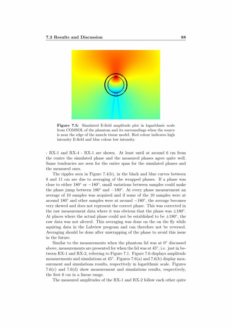
7.3 Results and Discussion 88
Figure 7.5: Simulated E-field amplitude plot in logarithmic scalefrom COMSOL of the phantom and its surroundings when the sourceis near the edge of the muscle tissue model. Red colour indicates highintensity E-field and blue colour low intensity.
- RX-1 and RX-4 - RX-1 are shown. At least until at around 6 cm fromthe centre the simulated phase and the measured phases agree quite well.Same tendencies are seen for the entire span for the simulated phases andthe measured ones.
The ripples seen in Figure 7.4(b), in the black and blue curves between8 and 11 cm are due to averaging of the wrapped phases. If a phase wasclose to either 180 or −180, small variations between samples could makethe phase jump between 180 and −180. At every phase measurement anaverage of 10 samples was acquired and if some of the 10 samples were ataround 180 and other samples were at around −180, the average becomesvery skewed and does not represent the correct phase. This was corrected inthe raw measurement data where it was obvious that the phase was ±180.At places where the actual phase could not be established to be ±180, theraw data was not altered. This averaging was done on the on the fly whileaquiring data in the Labview program and can therefore not be reversed.Averaging should be done after unwrapping of the phase to avoid this issuein the future.
Similar to the measurements when the phantom lid was at 0 discussedabove, measurements are presented for when the lid was at 45, i.e. just in be-tween RX-1 and RX-2, referring to Figure 7.1. Figure 7.6 displays amplitudemeasurements and simulations at 45. Figures 7.6(a) and 7.6(b) display mea-surement and simulations results, respectively in logarithmic scale. Figures7.6(c) and 7.6(d) show measurement and simulations results, respectively,the first 6 cm in a linear range.
The measured amplitudes of the RX-1 and RX-2 follow each other quite
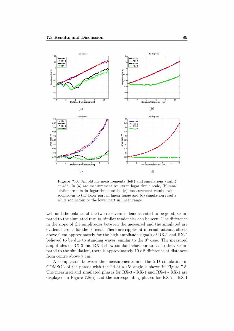
7.3 Results and Discussion 89
0 2 4 6 8 10−50
−40
−30
−20
−10
0
10
2045 degrees
Distance from center [cm]
Am
plitu
de [d
BV
]
RX−1RX−2RX−3RX−4
(a)
0 2 4 6 8 10−50
−40
−30
−20
−10
0
10
2045 degrees
Distance from center [cm]
Am
plitu
de [d
BV
]
RX−1RX−2RX−3RX−4
(b)
0 1 2 3 4 5 60
0.05
0.1
0.15
0.2
0.25
0.3
0.35
0.4
0.45
0.545 degrees
Distance from center [cm]
Am
plitu
de [V
]
RX−1RX−2RX−3RX−4
(c)
0 1 2 3 4 5 60
0.05
0.1
0.15
0.2
0.25
0.3
0.35
0.4
0.45
0.545 degrees
Distance from center [cm]
Am
plitu
de [V
]
RX−1RX−2RX−3RX−4
(d)
Figure 7.6: Amplitude measurements (left) and simulations (right)at 45. In (a) are measurement results in logarithmic scale, (b) sim-ulation results in logarithmic scale, (c) measurement results whilezoomed-in to the lower part in linear range and (d) simulation resultswhile zoomed-in to the lower part in linear range.
well and the balance of the two receivers is demonstrated to be good. Com-pared to the simulated results, similar tendencies can be seen. The differencein the slope of the amplitudes between the measured and the simulated areevident here as for the 0 case. There are ripples at internal antenna offsetsabove 9 cm approximately for the high amplitude signals of RX-1 and RX-2believed to be due to standing waves, similar to the 0 case. The measuredamplitudes of RX-3 and RX-4 show similar behaviour to each other. Com-pared to the simulation, there is approximately 10 dB difference at distancesfrom centre above 7 cm.
A comparison between the measurements and the 2-D simulation inCOMSOL of the phases with the lid at a 45 angle is shown in Figure 7.8.The measured and simulated phases for RX-3 - RX-1 and RX-4 - RX-1 aredisplayed in Figure 7.8(a) and the corresponding phases for RX-2 - RX-1
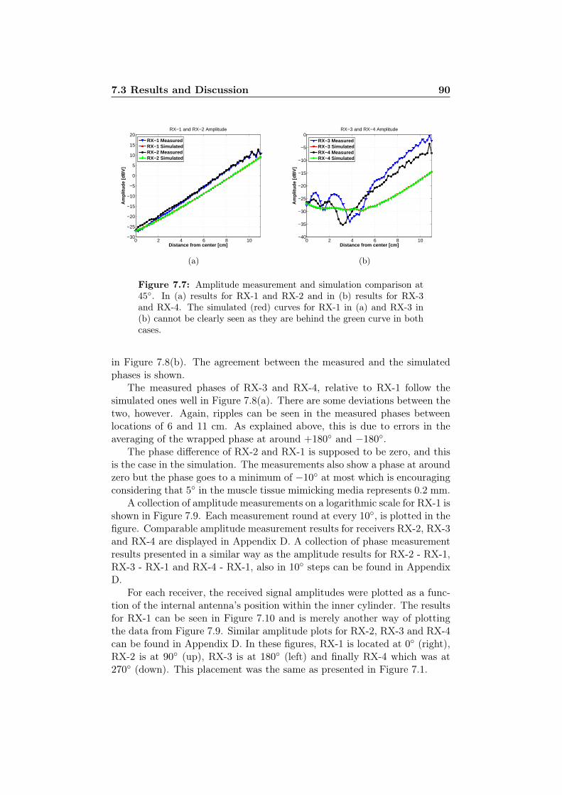
7.3 Results and Discussion 90
0 2 4 6 8 10−30
−25
−20
−15
−10
−5
0
5
10
15
20RX−1 and RX−2 Amplitude
Distance from center [cm]
Am
plitu
de [d
BV
]
RX−1 MeasuredRX−1 SimulatedRX−2 MeasuredRX−2 Simulated
(a)
0 2 4 6 8 10−40
−35
−30
−25
−20
−15
−10
−5
0RX−3 and RX−4 Amplitude
Distance from center [cm]
Am
plitu
de [d
BV
]
RX−3 MeasuredRX−3 SimulatedRX−4 MeasuredRX−4 Simulated
(b)
Figure 7.7: Amplitude measurement and simulation comparison at45. In (a) results for RX-1 and RX-2 and in (b) results for RX-3and RX-4. The simulated (red) curves for RX-1 in (a) and RX-3 in(b) cannot be clearly seen as they are behind the green curve in bothcases.
in Figure 7.8(b). The agreement between the measured and the simulatedphases is shown.
The measured phases of RX-3 and RX-4, relative to RX-1 follow thesimulated ones well in Figure 7.8(a). There are some deviations between thetwo, however. Again, ripples can be seen in the measured phases betweenlocations of 6 and 11 cm. As explained above, this is due to errors in theaveraging of the wrapped phase at around +180 and −180.
The phase difference of RX-2 and RX-1 is supposed to be zero, and thisis the case in the simulation. The measurements also show a phase at aroundzero but the phase goes to a minimum of −10 at most which is encouragingconsidering that 5 in the muscle tissue mimicking media represents 0.2 mm.
A collection of amplitude measurements on a logarithmic scale for RX-1 isshown in Figure 7.9. Each measurement round at every 10, is plotted in thefigure. Comparable amplitude measurement results for receivers RX-2, RX-3and RX-4 are displayed in Appendix D. A collection of phase measurementresults presented in a similar way as the amplitude results for RX-2 - RX-1,RX-3 - RX-1 and RX-4 - RX-1, also in 10 steps can be found in AppendixD.
For each receiver, the received signal amplitudes were plotted as a func-tion of the internal antenna’s position within the inner cylinder. The resultsfor RX-1 can be seen in Figure 7.10 and is merely another way of plottingthe data from Figure 7.9. Similar amplitude plots for RX-2, RX-3 and RX-4can be found in Appendix D. In these figures, RX-1 is located at 0 (right),RX-2 is at 90 (up), RX-3 is at 180 (left) and finally RX-4 which was at270 (down). This placement was the same as presented in Figure 7.1.
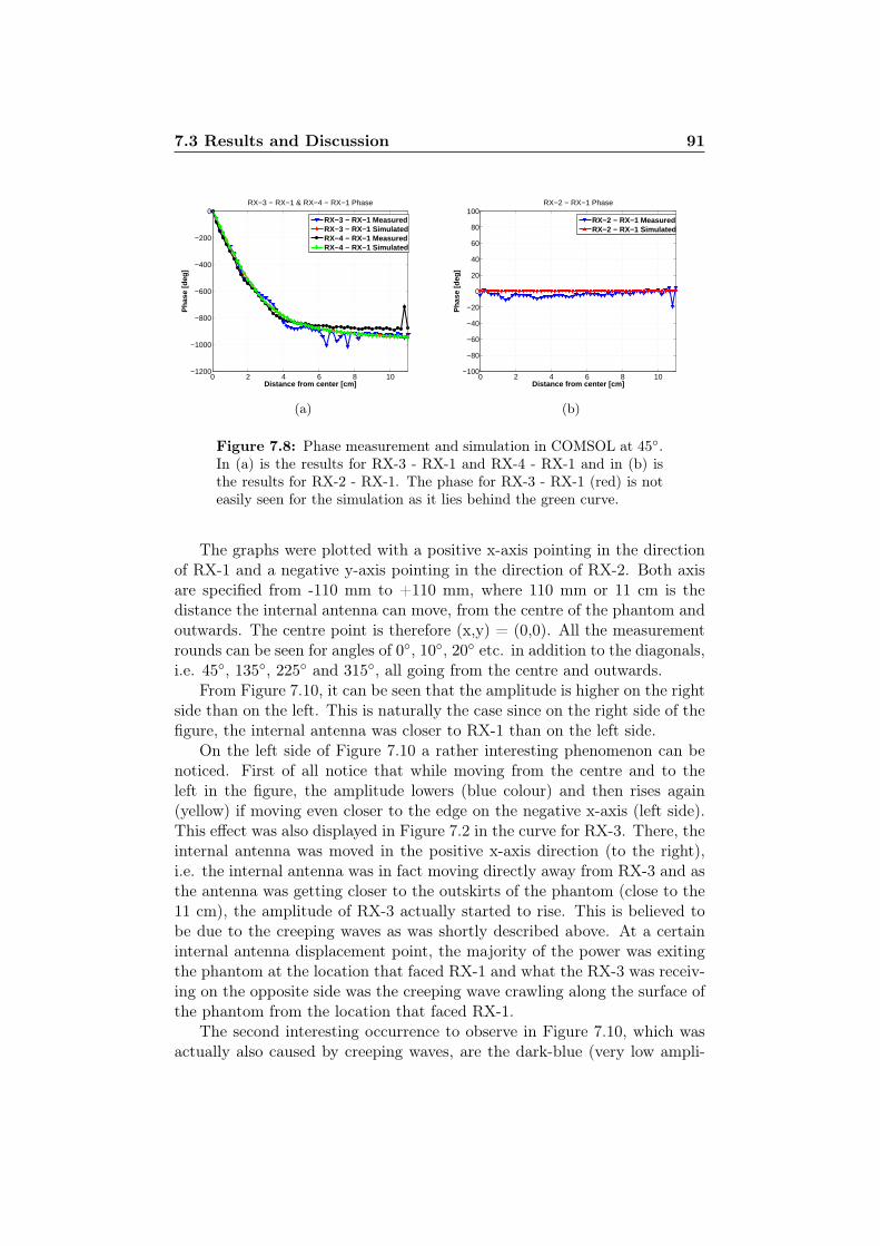
7.3 Results and Discussion 91
0 2 4 6 8 10−1200
−1000
−800
−600
−400
−200
0RX−3 − RX−1 & RX−4 − RX−1 Phase
Distance from center [cm]
Pha
se [d
eg]
RX−3 − RX−1 MeasuredRX−3 − RX−1 SimulatedRX−4 − RX−1 MeasuredRX−4 − RX−1 Simulated
(a)
0 2 4 6 8 10−100
−80
−60
−40
−20
0
20
40
60
80
100RX−2 − RX−1 Phase
Distance from center [cm]
Pha
se [d
eg]
RX−2 − RX−1 MeasuredRX−2 − RX−1 Simulated
(b)
Figure 7.8: Phase measurement and simulation in COMSOL at 45.In (a) is the results for RX-3 - RX-1 and RX-4 - RX-1 and in (b) isthe results for RX-2 - RX-1. The phase for RX-3 - RX-1 (red) is noteasily seen for the simulation as it lies behind the green curve.
The graphs were plotted with a positive x-axis pointing in the directionof RX-1 and a negative y-axis pointing in the direction of RX-2. Both axisare specified from -110 mm to +110 mm, where 110 mm or 11 cm is thedistance the internal antenna can move, from the centre of the phantom andoutwards. The centre point is therefore (x,y) = (0,0). All the measurementrounds can be seen for angles of 0, 10, 20 etc. in addition to the diagonals,i.e. 45, 135, 225 and 315, all going from the centre and outwards.
From Figure 7.10, it can be seen that the amplitude is higher on the rightside than on the left. This is naturally the case since on the right side of thefigure, the internal antenna was closer to RX-1 than on the left side.
On the left side of Figure 7.10 a rather interesting phenomenon can benoticed. First of all notice that while moving from the centre and to theleft in the figure, the amplitude lowers (blue colour) and then rises again(yellow) if moving even closer to the edge on the negative x-axis (left side).This effect was also displayed in Figure 7.2 in the curve for RX-3. There, theinternal antenna was moved in the positive x-axis direction (to the right),i.e. the internal antenna was in fact moving directly away from RX-3 and asthe antenna was getting closer to the outskirts of the phantom (close to the11 cm), the amplitude of RX-3 actually started to rise. This is believed tobe due to the creeping waves as was shortly described above. At a certaininternal antenna displacement point, the majority of the power was exitingthe phantom at the location that faced RX-1 and what the RX-3 was receiv-ing on the opposite side was the creeping wave crawling along the surface ofthe phantom from the location that faced RX-1.
The second interesting occurrence to observe in Figure 7.10, which wasactually also caused by creeping waves, are the dark-blue (very low ampli-
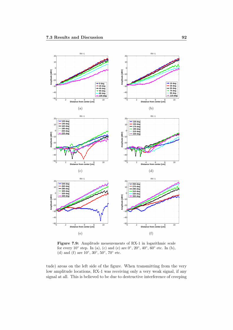
7.3 Results and Discussion 92
0 2 4 6 8 10−50
−40
−30
−20
−10
0
10
20RX−1
Distance from center [cm]
Am
plit
ud
e [d
BV
]
0 deg20 deg40 deg60 deg80 deg100 deg
(a)
0 2 4 6 8 10−50
−40
−30
−20
−10
0
10
20RX−1
Distance from center [cm]
Am
plit
ud
e [d
BV
]
10 deg30 deg50 deg70 deg90 deg110 deg
(b)
0 2 4 6 8 10−50
−40
−30
−20
−10
0
10
20RX−1
Distance from center [cm]
Am
plit
ud
e [d
BV
]
120 deg140 deg160 deg180 deg200 deg220 deg
(c)
0 2 4 6 8 10−50
−40
−30
−20
−10
0
10
20RX−1
Distance from center [cm]
Am
plit
ud
e [d
BV
]
130 deg150 deg170 deg190 deg210 deg230 deg
(d)
0 2 4 6 8 10−50
−40
−30
−20
−10
0
10
20RX−1
Distance from center [cm]
Am
plit
ud
e [d
BV
]
240 deg260 deg280 deg300 deg320 deg340 deg
(e)
0 2 4 6 8 10−50
−40
−30
−20
−10
0
10
20RX−1
Distance from center [cm]
Am
plit
ud
e [d
BV
]
250 deg270 deg290 deg310 deg330 deg350 deg
(f)
Figure 7.9: Amplitude measurements of RX-1 in logarithmic scalefor every 10 step. In (a), (c) and (e) are 0, 20, 40, 60 etc. In (b),(d) and (f) are 10, 30, 50, 70 etc.
tude) areas on the left side of the figure. When transmitting from the verylow amplitude locations, RX-1 was receiving only a very weak signal, if anysignal at all. This is believed to be due to destructive interference of creeping
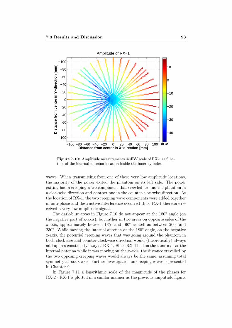
7.3 Results and Discussion 93
Distance from center in X−direction [mm]
Dis
tanc
e fr
om c
ente
r in
Y−d
irect
ion
[mm
]Amplitude of RX−1
−100 −80 −60 −40 −20 0 20 40 60 80 100
−100
−80
−60
−40
−20
0
20
40
60
80
100
dBV
−40
−30
−20
−10
0
10
Figure 7.10: Amplitude measurements in dBV scale of RX-1 as func-tion of the internal antenna location inside the inner cylinder.
waves. When transmitting from one of these very low amplitude locations,the majority of the power exited the phantom on its left side. The powerexiting had a creeping wave component that crawled around the phantom ina clockwise direction and another one in the counter-clockwise direction. Atthe location of RX-1, the two creeping wave components were added togetherin anti-phase and destructive interference occurred thus, RX-1 therefore re-ceived a very low amplitude signal.
The dark-blue areas in Figure 7.10 do not appear at the 180 angle (onthe negative part of x-axis), but rather in two areas on opposite sides of thex-axis, approximately between 135 and 160 as well as between 200 and230. While moving the internal antenna at the 180 angle, on the negativex-axis, the potential creeping waves that was going around the phantom inboth clockwise and counter-clockwise direction would (theoretically) alwaysadd up in a constructive way at RX-1. Since RX-1 lied on the same axis as theinternal antenna while it was moving on the x-axis, the distance travelled bythe two opposing creeping waves would always be the same, assuming totalsymmetry across x-axis. Further investigation on creeping waves is presentedin Chapter 9.
In Figure 7.11 a logarithmic scale of the magnitude of the phases forRX-2 - RX-1 is plotted in a similar manner as the previous amplitude figure.
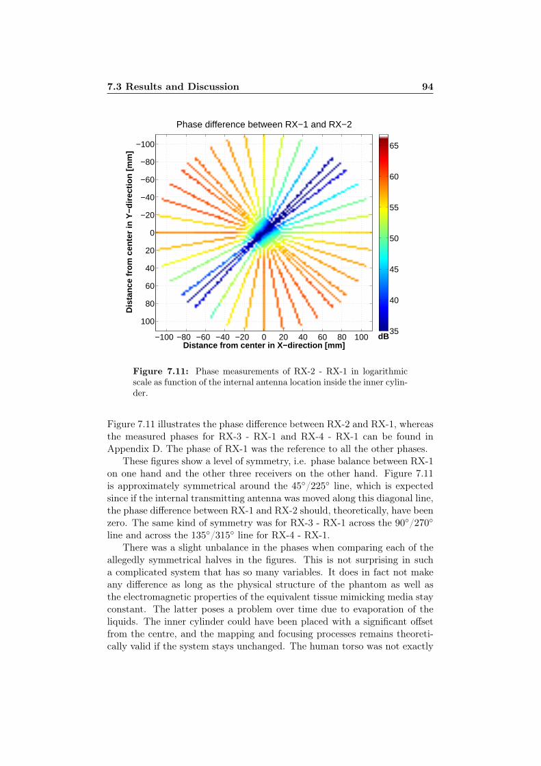
7.3 Results and Discussion 94
Distance from center in X−direction [mm]
Dis
tanc
e fr
om c
ente
r in
Y−d
irect
ion
[mm
]Phase difference between RX−1 and RX−2
−100 −80 −60 −40 −20 0 20 40 60 80 100
−100
−80
−60
−40
−20
0
20
40
60
80
100
dB35
40
45
50
55
60
65
Figure 7.11: Phase measurements of RX-2 - RX-1 in logarithmicscale as function of the internal antenna location inside the inner cylin-der.
Figure 7.11 illustrates the phase difference between RX-2 and RX-1, whereasthe measured phases for RX-3 - RX-1 and RX-4 - RX-1 can be found inAppendix D. The phase of RX-1 was the reference to all the other phases.
These figures show a level of symmetry, i.e. phase balance between RX-1on one hand and the other three receivers on the other hand. Figure 7.11is approximately symmetrical around the 45/225 line, which is expectedsince if the internal transmitting antenna was moved along this diagonal line,the phase difference between RX-1 and RX-2 should, theoretically, have beenzero. The same kind of symmetry was for RX-3 - RX-1 across the 90/270
line and across the 135/315 line for RX-4 - RX-1.There was a slight unbalance in the phases when comparing each of the
allegedly symmetrical halves in the figures. This is not surprising in sucha complicated system that has so many variables. It does in fact not makeany difference as long as the physical structure of the phantom as well asthe electromagnetic properties of the equivalent tissue mimicking media stayconstant. The latter poses a problem over time due to evaporation of theliquids. The inner cylinder could have been placed with a significant offsetfrom the centre, and the mapping and focusing processes remains theoreti-cally valid if the system stays unchanged. The human torso was not exactly

7.3 Results and Discussion 95
symmetrical and there was not a special requirement for the torso phan-tom to be symmetrical. However, it was preferred and attempted to havethe torso phantom and the microwave activation system as symmetrical aspossible during the initial measurements in order to verify the balance andsimilarities between the transmitters on one hand and the receivers on theother.
96
Chapter 8
System Measurements -Focusing
The essence of the external activation of pharmaceutical drugs with mi-crowaves, depends on the ability to induce EM power at certain areas insidethe body. A documented side effect of being irradiated by EM waves is that,unwanted heating of areas, other than intended, can occur. A method forreducing the side effects is, to superimpose EM waves from multiple sources,creating a focus point which inherently has higher amplitude than its sur-roundings, thus allowing for reduction of the radiated power from individualsources. This chapter describes the focusing experiments of the microwaveactivation system on the human torso phantom where measurement resultsare presented along with a discussion.
8.1 Measurement Setup
There are many similarities in the focusing case and in the mapping casewhen it comes to the measurement setup. Eight microwave absorbers werealso utilized here to minimize reflections from clutter. Clutter are objectsthat are not part of the microwave activation system and are dependent onthe current surroundings of the systems such as e.g. walls, chairs, tablesand shelves. During focusing, the position of the external antennas was un-changed in respect to the mapping and the phantom was the same. Thesetup was shown in Figure 7.1, but now with RX interchanged with TX.The component block diagram of the focusing setup was illustrated in Fig-ure 5.5. Now, the external antennas were connected to the outputs of thetransmitters, without the HPA boosting stage.
The four transmitters TX-1 to TX-4 were at the same locations as thereceivers RX-1 to RX-4 were in the mapping case, respectively, i.e. TX-1was at 0, TX-2 at 90 etc.
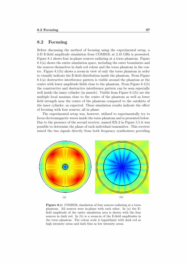
8.2 Focusing 97
8.2 Focusing
Before discussing the method of focusing using the experimental setup, a2-D E-field amplitude simulation from COMSOL at 2.45 GHz is presented.Figure 8.1 shows four in-phase sources radiating at a torso phantom. Figure8.1(a) shows the entire simulation space, including the outer boundaries andthe sources themselves in dark red colour and the torso phantom in the cen-tre. Figure 8.1(b) shows a zoom-in view of only the torso phantom in orderto visually indicate the E-field distribution inside the phantom. From Figure8.1(a) destructive interference pattern is visible around the phantom at thecentre with lower amplitude fields close to the phantom. From Figure 8.1(b)the constructive and destructive interference pattern can be seen especiallywell inside the inner cylinder (in muscle). Visible from Figure 8.1(b) are themultiple local maxima close to the centre of the phantom as well as lowerfield strength near the centre of the phantom compared to the outskirts ofthe inner cylinder, as expected. These simulation results indicate the effectof focusing with four sources, all in phase.
The experimental setup was, however, utilized to experimentally try tofocus electromagnetic waves inside the torso phantom and is presented below.Due to the presence of the second receiver, named RX-2 in Figure 5.5 it waspossible to determine the phase of each individual transmitter. This receivermixed the two signals directly from both frequency synthesizers providing
(a) (b)
Figure 8.1: COMSOL simulation of four sources radiating at a torsophantom. All sources were in-phase with each other. In (a) the E-field amplitude of the entire simulation area is shown with the foursources in dark red. In (b) is a zoom-in of the E-field amplitudes inthe torso phantom. The colour scale is logarithmic with dark red ashigh intensity areas and dark blue as low intensity areas.
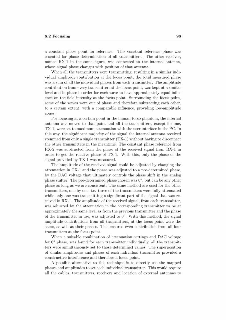
8.2 Focusing 98
a constant phase point for reference. This constant reference phase wasessential for phase determination of all transmitters. The other receiver,named RX-1 in the same figure, was connected to the internal antenna,whose signal phase changes with position of that antenna.
When all the transmitters were transmitting, resulting in a similar indi-vidual amplitude contribution at the focus point, the total measured phasewas a sum of all the individual phases from each transmitter. The amplitudecontribution from every transmitter, at the focus point, was kept at a similarlevel and in phase in order for each wave to have approximately equal influ-ence on the field intensity at the focus point. Surrounding the focus point,some of the waves were out of phase and therefore subtracting each other,to a certain extent, with a comparable influence, providing low-amplitudezones.
For focusing at a certain point in the human torso phantom, the internalantenna was moved to that point and all the transmitters, except for one,TX-1, were set to maximum attenuation with the user interface in the PC. Inthis way, the significant majority of the signal the internal antenna receivedstemmed from only a single transmitter (TX-1) without having to disconnectthe other transmitters in the meantime. The constant phase reference fromRX-2 was subtracted from the phase of the received signal from RX-1 inorder to get the relative phase of TX-1. With this, only the phase of thesignal provided by TX-1 was measured.
The amplitude of the received signal could be adjusted by changing theattenuation in TX-1 and the phase was adjusted to a pre-determined phase,by the DAC voltage that ultimately controls the phase shift in the analogphase shifter. The pre-determined phase chosen was 0, but can be any otherphase as long as we are consistent. The same method are used for the othertransmitters, one by one, i.e. three of the transmitters were fully attenuatedwhile only one was transmitting a significant part of the signal that was re-ceived in RX-1. The amplitude of the received signal, from each transmitter,was adjusted by the attenuation in the corresponding transmitter to be atapproximately the same level as from the previous transmitter and the phaseof the transmitter in use, was adjusted to 0. With this method, the signalamplitude contributions from all transmitters, at the focus point were thesame, as well as their phases. This ensured even contribution from all fourtransmitters at the focus point.
When a suitable combination of attenuation settings and DAC voltagefor 0 phase, was found for each transmitter individually, all the transmit-ters were simultaneously set to those determined values. The superpositionof similar amplitudes and phases of each individual transmitter provided aconstructive interference and therefore a focus point.
A possible alternative to this technique is to directly use the mappedphases and amplitudes to set each individual transmitter. This would requireall the cables, transmitters, receivers and location of external antennas to
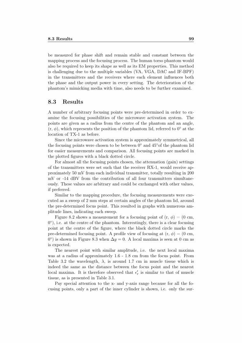
8.3 Results 99
be measured for phase shift and remain stable and constant between themapping process and the focusing process. The human torso phantom wouldalso be required to keep its shape as well as its EM properties. This methodis challenging due to the multiple variables (VA, VGA, DAC and IF-BPF)in the transmitters and the receivers where each element influences boththe phase and the output power in every setting. The deterioration of thephantom’s mimicking media with time, also needs to be further examined.
8.3 Results
A number of arbitrary focusing points were pre-determined in order to ex-amine the focusing possibilities of the microwave activation system. Thepoints are given as a radius from the centre of the phantom and an angle,(r, φ), which represents the position of the phantom lid, referred to 0 at thelocation of TX-1 as before.
Since the microwave activation system is approximately symmetrical, allthe focusing points were chosen to be between 0 and 45of the phantom lidfor easier measurements and comparison. All focusing points are marked inthe plotted figures with a black dotted circle.
For almost all the focusing points chosen, the attenuation (gain) settingsof the transmitters were set such that the receiver RX-1, would receive ap-proximately 50 mV from each individual transmitter, totally resulting in 200mV or -14 dBV from the contribution of all four transmitters simultane-ously. These values are arbitrary and could be exchanged with other values,if preferred.
Similar to the mapping procedure, the focusing measurements were exe-cuted as a sweep of 2 mm steps at certain angles of the phantom lid, aroundthe pre-determined focus point. This resulted in graphs with numerous am-plitude lines, indicating each sweep.
Figure 8.2 shows a measurement for a focusing point of (r, φ) = (0 cm,0), i.e. at the centre of the phantom. Interestingly, there is a clear focusingpoint at the centre of the figure, where the black dotted circle marks thepre-determined focusing point. A profile view of focusing at (r, φ) = (0 cm,0) is shown in Figure 8.3 when ∆y = 0. A local maxima is seen at 0 cm asis expected.
The nearest point with similar amplitude, i.e. the next local maximawas at a radius of approximately 1.6 - 1.8 cm from the focus point. FromTable 3.2 the wavelength, λ, is around 1.7 cm in muscle tissue which isindeed the same as the distance between the focus point and the nearestlocal maxima. It is therefore observed that ε′r is similar to that of muscletissue, as is presented in Table 3.1.
Pay special attention to the x- and y-axis range because for all the fo-cusing points, only a part of the inner cylinder is shown, i.e. only the sur-
8.3 Results 100
roundings of each of the focus points was examined.The next focus point was set to (r, φ) = (2 cm, 20) and the result is
shown in Figure 8.4. Again, a clear focus point is seen at the location of thepre-determined focusing point marked with black circle. The nearest pointwith similar amplitude was at a radius of 2.1 cm from the focus point. Thenearest surroundings to the focus point were considerably lower in amplitudethan the focus point itself. Notice that, the scale for this figure is not the
Distance from center in X−direction [mm]
Dis
tanc
e fr
om c
ente
r in
Y−d
irect
ion
[mm
]
Amplitude of RX−1
−40 −30 −20 −10 0 10 20 30 40
−40
−30
−20
−10
0
10
20
30
40dBV
−30
−25
−20
−15
−10
−5
Figure 8.2: Focusing at the centre of the phantom (r, φ) = (0 cm,0).
−40 −20 0 20 40−30
−25
−20
−15
−10
−5
0∆ y = 0 Profile
Distance from center [cm]
Am
plit
ud
e [d
BV
]
∆ y = 0
Figure 8.3: Focusing at the centre of the phantom (r, φ) = (0 cm,0). A profile view when ∆y = 0.
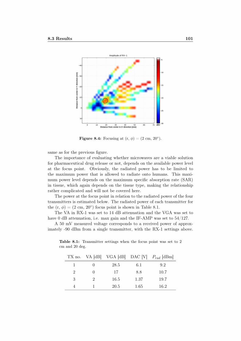
8.3 Results 101
Distance from center in X−direction [mm]
Dis
tanc
e fr
om c
ente
r in
Y−d
irect
ion
[mm
]
Amplitude of RX−1
0 10 20 30 40 50 60 70
−40
−30
−20
−10
0
10
dBV−30
−25
−20
−15
−10
−5
Figure 8.4: Focusing at (r, φ) = (2 cm, 20).
same as for the previous figure.The importance of evaluating whether microwaves are a viable solution
for pharmaceutical drug release or not, depends on the available power levelat the focus point. Obviously, the radiated power has to be limited tothe maximum power that is allowed to radiate onto humans. This maxi-mum power level depends on the maximum specific absorption rate (SAR)in tissue, which again depends on the tissue type, making the relationshiprather complicated and will not be covered here.
The power at the focus point in relation to the radiated power of the fourtransmitters is estimated below. The radiated power of each transmitter forthe (r, φ) = (2 cm, 20) focus point is shown in Table 8.1.
The VA in RX-1 was set to 14 dB attenuation and the VGA was set tohave 0 dB attenuation, i.e. max gain and the IF-AMP was set to 54/127.
A 50 mV measured voltage corresponds to a received power of approx-imately -90 dBm from a single transmitter, with the RX-1 settings above.
Table 8.1: Transmitter settings when the focus point was set to 2cm and 20 deg.
TX no. VA [dB] VGA [dB] DAC [V] Prad [dBm]
1 0 28.5 6.1 9.2
2 0 17 8.8 10.7
3 2 16.5 1.37 19.7
4 1 20.5 1.65 16.2
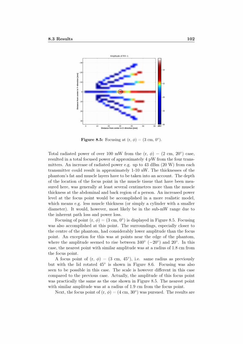
8.3 Results 102
Distance from center in X−direction [mm]
Dis
tanc
e fr
om c
ente
r in
Y−d
irect
ion
[mm
]
Amplitude of RX−1
0 10 20 30 40 50 60
−30
−20
−10
0
10
20
30
dBV−30
−25
−20
−15
−10
Figure 8.5: Focusing at (r, φ) = (3 cm, 0).
Total radiated power of over 100 mW from the (r, φ) = (2 cm, 20) case,resulted in a total focused power of approximately 4 pW from the four trans-mitters. An increase of radiated power e.g. up to 43 dBm (20 W) from eachtransmitter could result in approximately 1-10 nW. The thicknesses of thephantom’s fat and muscle layers have to be taken into an account. The depthof the location of the focus point in the muscle tissue that have been mea-sured here, was generally at least several centimetres more than the musclethickness at the abdominal and back region of a person. An increased powerlevel at the focus point would be accomplished in a more realistic model,which means e.g. less muscle thickness (or simply a cylinder with a smallerdiameter). It would, however, most likely be in the sub-mW range due tothe inherent path loss and power loss.
Focusing of point (r, φ) = (3 cm, 0) is displayed in Figure 8.5. Focusingwas also accomplished at this point. The surroundings, especially closer tothe centre of the phantom, had considerably lower amplitude than the focuspoint. An exception for this was at points near the edge of the phantom,where the amplitude seemed to rise between 340 (−20) and 20. In thiscase, the nearest point with similar amplitude was at a radius of 1.8 cm fromthe focus point.
A focus point of (r, φ) = (3 cm, 45), i.e. same radius as previouslybut with the lid rotated 45 is shown in Figure 8.6. Focusing was alsoseen to be possible in this case. The scale is however different in this casecompared to the previous case. Actually, the amplitude of this focus pointwas practically the same as the one shown in Figure 8.5. The nearest pointwith similar amplitude was at a radius of 1.9 cm from the focus point.
Next, the focus point of (r, φ) = (4 cm, 30) was pursued. The results are
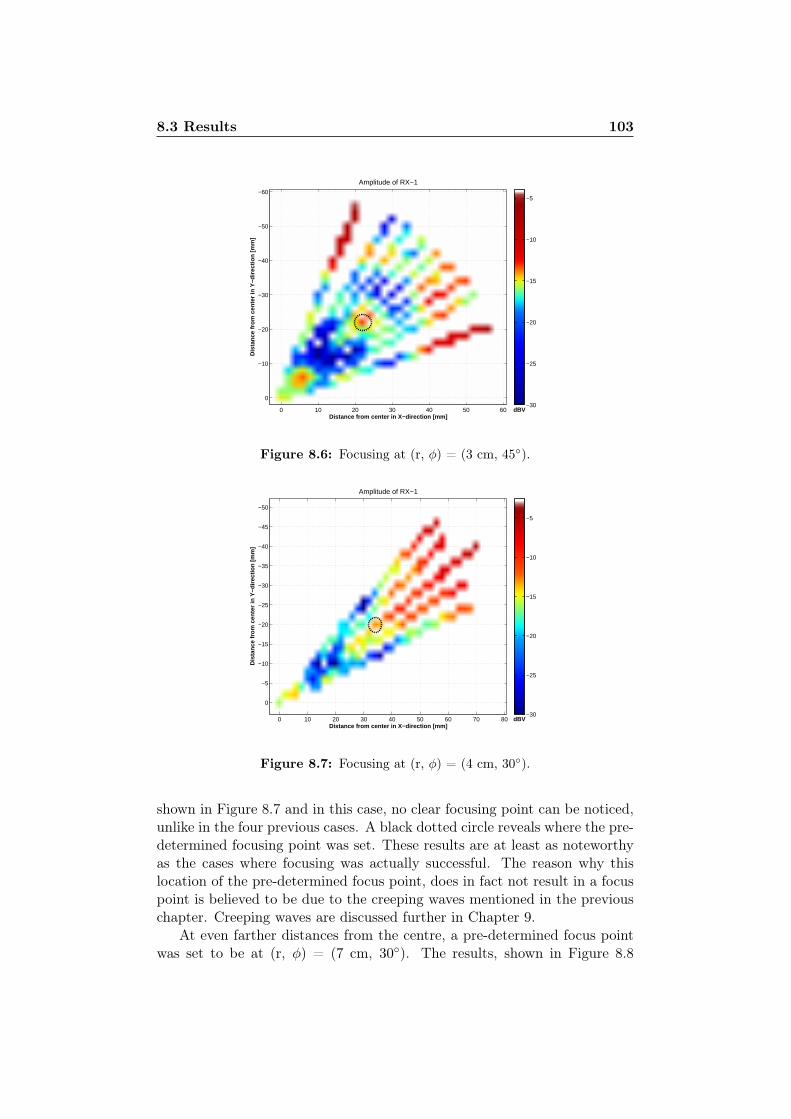
8.3 Results 103
Distance from center in X−direction [mm]
Dis
tanc
e fr
om c
ente
r in
Y−d
irect
ion
[mm
]
Amplitude of RX−1
0 10 20 30 40 50 60
−60
−50
−40
−30
−20
−10
0
dBV−30
−25
−20
−15
−10
−5
Figure 8.6: Focusing at (r, φ) = (3 cm, 45).
Distance from center in X−direction [mm]
Dis
tanc
e fr
om c
ente
r in
Y−d
irect
ion
[mm
]
Amplitude of RX−1
0 10 20 30 40 50 60 70 80
−50
−45
−40
−35
−30
−25
−20
−15
−10
−5
0
dBV−30
−25
−20
−15
−10
−5
Figure 8.7: Focusing at (r, φ) = (4 cm, 30).
shown in Figure 8.7 and in this case, no clear focusing point can be noticed,unlike in the four previous cases. A black dotted circle reveals where the pre-determined focusing point was set. These results are at least as noteworthyas the cases where focusing was actually successful. The reason why thislocation of the pre-determined focus point, does in fact not result in a focuspoint is believed to be due to the creeping waves mentioned in the previouschapter. Creeping waves are discussed further in Chapter 9.
At even farther distances from the centre, a pre-determined focus pointwas set to be at (r, φ) = (7 cm, 30). The results, shown in Figure 8.8
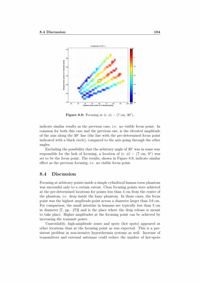
8.4 Discussion 104
Distance from center in X−direction [mm]
Dis
tanc
e fr
om c
ente
r in
Y−d
irect
ion
[mm
]
Amplitude of RX−1
20 30 40 50 60 70 80 90 100
−70
−60
−50
−40
−30
−20
−10dBV
−30
−25
−20
−15
−10
−5
0
Figure 8.8: Focusing at (r, φ) = (7 cm, 30).
indicate similar results as the previous case, i.e. no visible focus point. Incommon for both this case and the previous one, is the elevated amplitudeof the axis along the 30 line (the line with the pre-determined focus pointindicated with a black circle), compared to the axis going through the otherangles.
Excluding the possibility that the arbitrary angle of 30 was in some wayresponsible for the lack of focusing, a location of (r, φ) = (7 cm, 0) wasset to be the focus point. The results, shown in Figure 8.9, indicate similareffect as the previous focusing, i.e. no visible focus point.
8.4 Discussion
Focusing at arbitrary points inside a simple cylindrical human torso phantomwas successful only to a certain extent. Clear focusing points were achievedat the pre-determined locations for points less than 4 cm from the centre ofthe phantom, i.e. deep inside the lossy phantom. In those cases, the focuspoint was the highest amplitude-point across a diameter larger than 3.6 cm.For comparison, the small intestine in humans are typically less than 3 cmin diameter [7, pp. 272] and is the place where the drug release is meantto take place. Higher amplitudes at the focusing point can be achieved byincreasing the transmit power.
Unavoidably, high-amplitude zones and spots (hot spots) appeared atother locations than at the focusing point as was expected. This is a per-sistent problem in non-invasive hyperthermia systems as well. Increase oftransmitters and external antennas could reduce the number of hot-spots
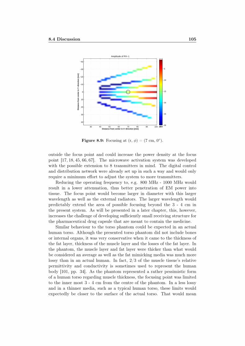
8.4 Discussion 105
Distance from center in X−direction [mm]
Dis
tanc
e fr
om c
ente
r in
Y−d
irect
ion
[mm
]
Amplitude of RX−1
30 40 50 60 70 80 90 100
−40
−30
−20
−10
0
10
20
30
40
dBV−30
−25
−20
−15
−10
−5
Figure 8.9: Focusing at (r, φ) = (7 cm, 0).
outside the focus point and could increase the power density at the focuspoint [17, 18, 45, 66, 67]. The microwave activation system was developedwith the possible extension to 8 transmitters in mind. The digital controland distribution network were already set up in such a way and would onlyrequire a minimum effort to adjust the system to more transmitters.
Reducing the operating frequency to, e.g. 800 MHz - 1000 MHz wouldresult in a lower attenuation, thus better penetration of EM power intotissue. The focus point would become larger in diameter with this largerwavelength as well as the external radiators. The larger wavelength wouldpredictably extend the area of possible focusing beyond the 3 - 4 cm inthe present system. As will be presented in a later chapter, this, however,increases the challenge of developing sufficiently small receiving structure forthe pharmaceutical drug capsule that are meant to contain the medicine.
Similar behaviour to the torso phantom could be expected in an actualhuman torso. Although the presented torso phantom did not include bonesor internal organs, it was very conservative when it came to the thickness ofthe fat layer, thickness of the muscle layer and the losses of the fat layer. Inthe phantom, the muscle layer and fat layer were thicker than what wouldbe considered an average as well as the fat mimicking media was much morelossy than in an actual human. In fact, 2/3 of the muscle tissue’s relativepermittivity and conductivity is sometimes used to represent the humanbody [101, pp. 34]. As the phantom represented a rather pessimistic formof a human torso regarding muscle thickness, the focusing point was limitedto the inner most 3 - 4 cm from the centre of the phantom. In a less lossyand in a thinner media, such as a typical human torso, these limits wouldexpectedly be closer to the surface of the actual torso. That would mean
8.4 Discussion 106
that there is probably a larger zone inside an actual human that creation ofa focus point would be possible. Also a higher-amplitude focus point wouldalso be accomplished in a human due to less losses and thinner structures.
The simple 2-D model in COMSOL shows good agreement with the ex-perimental dual-layered phantom. This implies that a 2-D model in COM-SOL of a actual human torso slice, of the patient in question, could possiblybe utilized for predicting and adjusting the phases and amplitudes of theexternal transmitters to obtain a pre-determined focus point.
107
Chapter 9
Creeping Waves
In the previous chapters on system measurements for the mapping and thefocusing, creeping waves were presented. Creeping waves is a name of a caseof diffraction where an electromagnetic wave can propagate along a curvedpath into a shadow zone (out of line of sight). In this chapter the behaviourof the creeping waves and their effect on external microwave activation ofpharmaceutical drug release are examined.
9.1 Creeping Wave Behaviour
A similar behaviour to the creeping waves, described in the previous chaptersfor the phantom, would be expected when transmitting from within, or at,a human torso, resulting in some noteworthy effects.
The principle of the creeping waves on a biological tissue equivalent phan-tom is presented in a simplistic manner in Figure 9.1. Figure 9.1(a) indicateshow the power reaches receivers RX-1 and RX-3 on opposite sides when theinternal antenna is at the centre of the phantom, with blue and red arrowswhen only two main paths are considered. In this case, power would beradiated radially away from the internal antenna to RX-1 and RX-3. Figure9.1(b) shows a case when the internal antenna is offset from the centre enoughfor the creeping waves to overshadow the direct waves as was discussed inChapter 7. This was at least 3.2 cm offset from the centre of the phantomwhen the lid was positioned at 0. In the creeping wave case, the majorityof the power would exit the phantom, facing RX-1. Creeping waves followthe curvature of the phantom and would ultimately be received by RX-3. Apart of the power would also travel in the direct path towards RX-3 but itsamplitude would be lower than from the creeping wave. The waves can alsotravel along other paths, but only these three paths are considered in this ex-ample. The creeping waves do not strictly confine themselves to boundariesor surfaces, but also travel in both media, with a different velocity due toa different permittivity. Figure 9.1 shows only the principle of the creeping
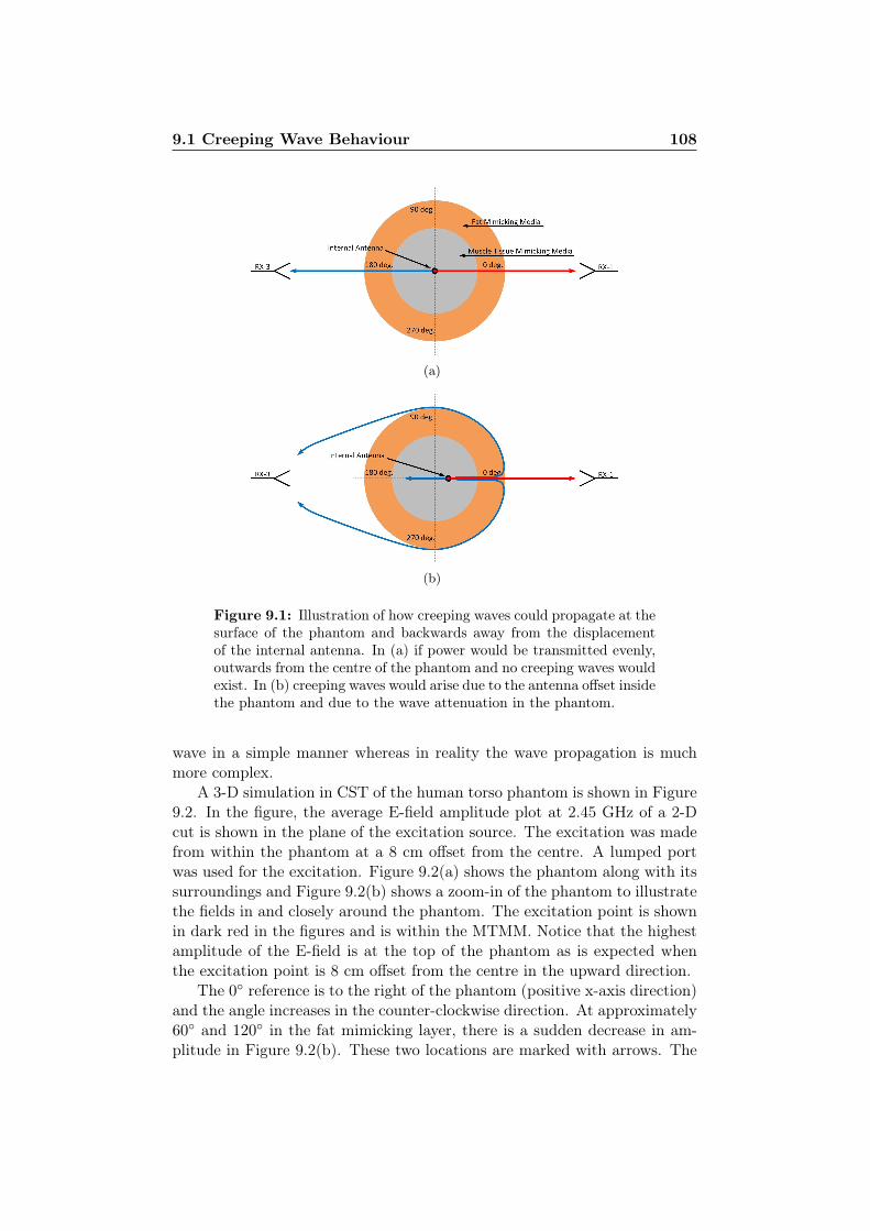
9.1 Creeping Wave Behaviour 108
(a)
(b)
Figure 9.1: Illustration of how creeping waves could propagate at thesurface of the phantom and backwards away from the displacementof the internal antenna. In (a) if power would be transmitted evenly,outwards from the centre of the phantom and no creeping waves wouldexist. In (b) creeping waves would arise due to the antenna offset insidethe phantom and due to the wave attenuation in the phantom.
wave in a simple manner whereas in reality the wave propagation is muchmore complex.
A 3-D simulation in CST of the human torso phantom is shown in Figure9.2. In the figure, the average E-field amplitude plot at 2.45 GHz of a 2-Dcut is shown in the plane of the excitation source. The excitation was madefrom within the phantom at a 8 cm offset from the centre. A lumped portwas used for the excitation. Figure 9.2(a) shows the phantom along with itssurroundings and Figure 9.2(b) shows a zoom-in of the phantom to illustratethe fields in and closely around the phantom. The excitation point is shownin dark red in the figures and is within the MTMM. Notice that the highestamplitude of the E-field is at the top of the phantom as is expected whenthe excitation point is 8 cm offset from the centre in the upward direction.
The 0 reference is to the right of the phantom (positive x-axis direction)and the angle increases in the counter-clockwise direction. At approximately60 and 120 in the fat mimicking layer, there is a sudden decrease in am-plitude in Figure 9.2(b). These two locations are marked with arrows. The
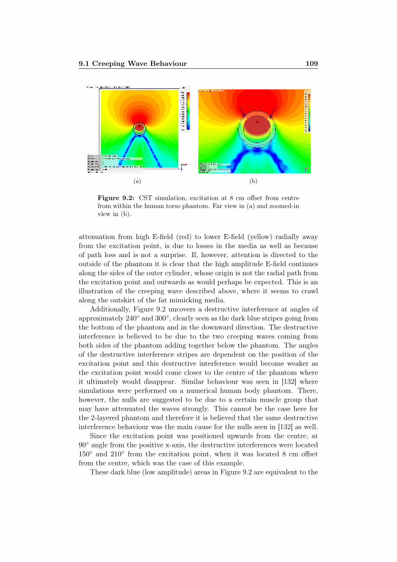
9.1 Creeping Wave Behaviour 109
(a) (b)
Figure 9.2: CST simulation, excitation at 8 cm offset from centrefrom within the human torso phantom. Far view in (a) and zoomed-inview in (b).
attenuation from high E-field (red) to lower E-field (yellow) radially awayfrom the excitation point, is due to losses in the media as well as becauseof path loss and is not a surprise. If, however, attention is directed to theoutside of the phantom it is clear that the high amplitude E-field continuesalong the sides of the outer cylinder, whose origin is not the radial path fromthe excitation point and outwards as would perhaps be expected. This is anillustration of the creeping wave described above, where it seems to crawlalong the outskirt of the fat mimicking media.
Additionally, Figure 9.2 uncovers a destructive interference at angles ofapproximately 240 and 300, clearly seen as the dark blue stripes going fromthe bottom of the phantom and in the downward direction. The destructiveinterference is believed to be due to the two creeping waves coming fromboth sides of the phantom adding together below the phantom. The anglesof the destructive interference stripes are dependent on the position of theexcitation point and this destructive interference would become weaker asthe excitation point would come closer to the centre of the phantom whereit ultimately would disappear. Similar behaviour was seen in [132] wheresimulations were performed on a numerical human body phantom. There,however, the nulls are suggested to be due to a certain muscle group thatmay have attenuated the waves strongly. This cannot be the case here forthe 2-layered phantom and therefore it is believed that the same destructiveinterference behaviour was the main cause for the nulls seen in [132] as well.
Since the excitation point was positioned upwards from the centre, at90 angle from the positive x-axis, the destructive interferences were located150 and 210 from the excitation point, when it was located 8 cm offsetfrom the centre, which was the case of this example.
These dark blue (low amplitude) areas in Figure 9.2 are equivalent to the
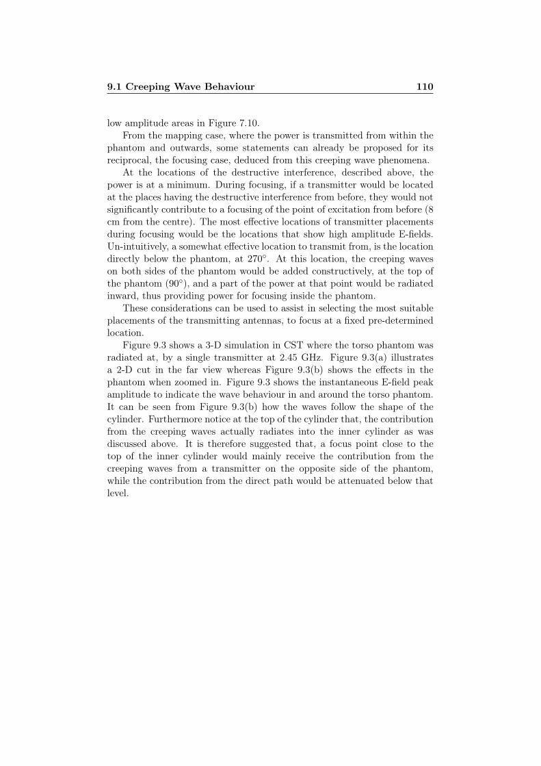
9.1 Creeping Wave Behaviour 110
low amplitude areas in Figure 7.10.From the mapping case, where the power is transmitted from within the
phantom and outwards, some statements can already be proposed for itsreciprocal, the focusing case, deduced from this creeping wave phenomena.
At the locations of the destructive interference, described above, thepower is at a minimum. During focusing, if a transmitter would be locatedat the places having the destructive interference from before, they would notsignificantly contribute to a focusing of the point of excitation from before (8cm from the centre). The most effective locations of transmitter placementsduring focusing would be the locations that show high amplitude E-fields.Un-intuitively, a somewhat effective location to transmit from, is the locationdirectly below the phantom, at 270. At this location, the creeping waveson both sides of the phantom would be added constructively, at the top ofthe phantom (90), and a part of the power at that point would be radiatedinward, thus providing power for focusing inside the phantom.
These considerations can be used to assist in selecting the most suitableplacements of the transmitting antennas, to focus at a fixed pre-determinedlocation.
Figure 9.3 shows a 3-D simulation in CST where the torso phantom wasradiated at, by a single transmitter at 2.45 GHz. Figure 9.3(a) illustratesa 2-D cut in the far view whereas Figure 9.3(b) shows the effects in thephantom when zoomed in. Figure 9.3 shows the instantaneous E-field peakamplitude to indicate the wave behaviour in and around the torso phantom.It can be seen from Figure 9.3(b) how the waves follow the shape of thecylinder. Furthermore notice at the top of the cylinder that, the contributionfrom the creeping waves actually radiates into the inner cylinder as wasdiscussed above. It is therefore suggested that, a focus point close to thetop of the inner cylinder would mainly receive the contribution from thecreeping waves from a transmitter on the opposite side of the phantom,while the contribution from the direct path would be attenuated below thatlevel.
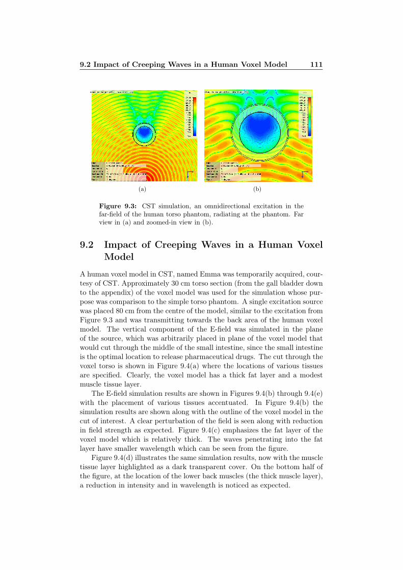
9.2 Impact of Creeping Waves in a Human Voxel Model 111
(a) (b)
Figure 9.3: CST simulation, an omnidirectional excitation in thefar-field of the human torso phantom, radiating at the phantom. Farview in (a) and zoomed-in view in (b).
9.2 Impact of Creeping Waves in a Human VoxelModel
A human voxel model in CST, named Emma was temporarily acquired, cour-tesy of CST. Approximately 30 cm torso section (from the gall bladder downto the appendix) of the voxel model was used for the simulation whose pur-pose was comparison to the simple torso phantom. A single excitation sourcewas placed 80 cm from the centre of the model, similar to the excitation fromFigure 9.3 and was transmitting towards the back area of the human voxelmodel. The vertical component of the E-field was simulated in the planeof the source, which was arbitrarily placed in plane of the voxel model thatwould cut through the middle of the small intestine, since the small intestineis the optimal location to release pharmaceutical drugs. The cut through thevoxel torso is shown in Figure 9.4(a) where the locations of various tissuesare specified. Clearly, the voxel model has a thick fat layer and a modestmuscle tissue layer.
The E-field simulation results are shown in Figures 9.4(b) through 9.4(e)with the placement of various tissues accentuated. In Figure 9.4(b) thesimulation results are shown along with the outline of the voxel model in thecut of interest. A clear perturbation of the field is seen along with reductionin field strength as expected. Figure 9.4(c) emphasizes the fat layer of thevoxel model which is relatively thick. The waves penetrating into the fatlayer have smaller wavelength which can be seen from the figure.
Figure 9.4(d) illustrates the same simulation results, now with the muscletissue layer highlighted as a dark transparent cover. On the bottom half ofthe figure, at the location of the lower back muscles (the thick muscle layer),a reduction in intensity and in wavelength is noticed as expected.
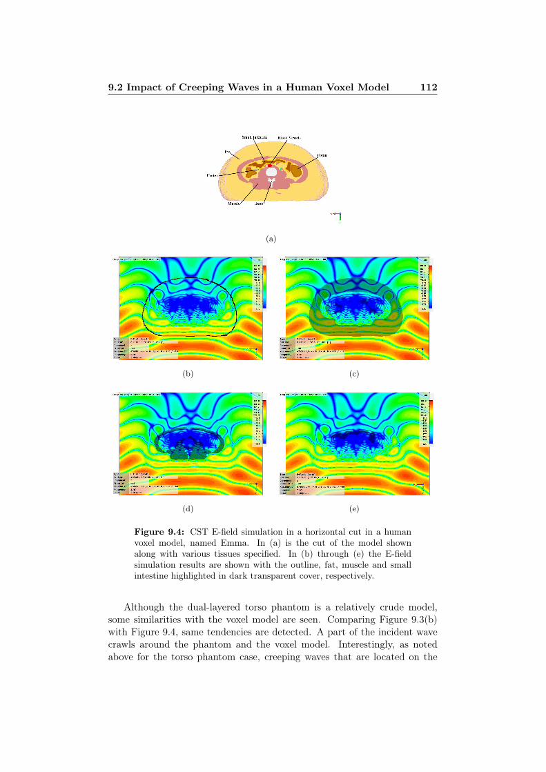
9.2 Impact of Creeping Waves in a Human Voxel Model 112
(a)
(b) (c)
(d) (e)
Figure 9.4: CST E-field simulation in a horizontal cut in a humanvoxel model, named Emma. In (a) is the cut of the model shownalong with various tissues specified. In (b) through (e) the E-fieldsimulation results are shown with the outline, fat, muscle and smallintestine highlighted in dark transparent cover, respectively.
Although the dual-layered torso phantom is a relatively crude model,some similarities with the voxel model are seen. Comparing Figure 9.3(b)with Figure 9.4, same tendencies are detected. A part of the incident wavecrawls around the phantom and the voxel model. Interestingly, as notedabove for the torso phantom case, creeping waves that are located on the
9.3 Creeping Wave’s Influence on Focusing 113
front side (upper half) of the voxel model, result in a wave transmissioninwards into the voxel model. This is perhaps most clearly illustrated belowthe abdominal muscle layer, in Figure 9.4(d). A similar effect is displayed atthe top of the cylindrical muscle layer, in Figure 9.3(b), where waves werebeing transmitted into the phantom, from the top (on the other side of thesource).
This behaviour of the E-field in the voxel model, which was alreadypredicted by the cylindrical torso phantom, suggests that creeping wavesalso need to be taken into consideration in actual human torsos. Figure9.4(e) illustrates the location of the small intestine along with the E-fieldsimulation results. Since the location of drug release is meant to be in thesmall intestine, the figure reveals that the main contribution of the E-fieldat the location of the small intestine, from an exciting wave coming frombehind of the model, would mostly be due to creeping waves.
9.3 Creeping Wave’s Influence on Focusing
Let’s consider two separate cases of having four sources transmitting at thephantom for focusing. The first case is where the contribution of the receivedsignal inside the phantom is from the direct path of all the transmitters, aswould be the case when the receiving internal antenna (focus point) wouldbe close to the centre of the phantom. The second case is when the internalantenna is closer to an edge of the phantom and assuming that a part ofthe received signal stems from an indirect path due to creeping waves. Forsimplicity, let’s only consider points on the positive x-axis, i.e. from thecentre of the phantom and towards TX-1. The setup was shown in Figure7.1 where RX are interchanged with TX.
For the first case, imagine a pre-determined focus point close to thecentre of the phantom, e.g. (r, φ) = (1 cm, 0). When measuring thereceived amplitude to the left (towards the centre) of the focus point stepby step (i.e. 0.8 cm, 0.6 cm, 0.4 cm etc.), the contribution from TX-3 wouldincrease and the contribution from TX-1 would decrease. When measuringthe amplitude to the right of the focus point, the opposite would happen,i.e. the contribution from TX-3 would decrease and the contribution fromTX-1 would increase.
For the second case, imagine a pre-determined focus point closer to theedge of the phantom, e.g. (r, φ) = (7 cm, 0). At the left side (near thecentre) of the focus point, the contribution from TX-3 would reduce as wellas the contribution from TX-1 since both waves are essentially radiating fromthe edge of the phantom that faces TX-1. Oppositely, the contribution fromboth TX-3 and TX-1 would increase when moving towards the edge of thephantom. This continuous increase is seen in Figures 8.7 and 8.8 in the 30
line (line of the pre-determined focus point) where no focusing is found.
9.4 Creeping Wave Verification Experiment 114
These behaviours around the focus point of the first and the second caseare believed to be the reasons why the results from first case show an evidentfocus point and the second case does not.
9.4 Creeping Wave Verification Experiment
An experiment was arranged in order to verify the previous creeping wavediscussions. The internal antenna was fixed at a 8 cm offset from the centre ofphantom, at 0 (directly in front of TX-1’s location from before). Microwaveabsorbers were placed around the phantom to reduce any reflections. Asingle transmitter, TX-3, was used for the excitation and was located on theopposite side.
Three cases were tested. In the first case, the TX-3 was simply transmit-ting unobstructed onto the phantom. In the second case a 3 cm thick blockof a layered planar microwave absorber was placed in front of the phantom,facing the transmitter TX-3, touching the surface of the outer cylinder ofthe phantom. This setup is shown in Figure 9.5(a). Figure 9.5(b) shows thethird case where the same planar microwave absorber was placed behind thephantom, relative to TX-3. Everything was kept unchanged for the threecases with the exception of the placement of the planar microwave absorber.Since the planar microwave absorber has several layers of various EM prop-erties, it was made sure that in both case 2 and case 3, the same layer wasfacing the phantom.
The reference case, which is the first case where no planar absorber wasused, produced approximately 50 mV in the receiver. In the second case,where the absorber was placed directly in front of the phantom, only a minorchange was found in the received signal which read around 48 mV. Themost noteworthy results were generated by the third case where the planarabsorber was located behind the phantom. Here the signal level droppedto 5 mV. It is believed that there are creeping waves propagating aroundthe phantom, originating from TX-3 and a part of these creeping waves areadded in phase behind the phantom, at the location of the layered absorberin case three. The layered microwave absorber, heavily attenuates the fieldsthat otherwise would be transmitted into the phantom, thus the receivedsignal was significantly reduced.
These results support the previous claims of creeping waves crawlingaround the phantom and are transmitted inwards, from the opposite side ofthe source.
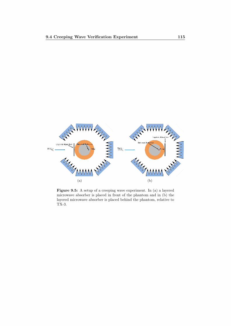
9.4 Creeping Wave Verification Experiment 115
(a) (b)
Figure 9.5: A setup of a creeping wave experiment. In (a) a layeredmicrowave absorber is placed in front of the phantom and in (b) thelayered microwave absorber is placed behind the phantom, relative toTX-3.
116
Chapter 10
Performance-Reduction Factors
In this chapter, deviations and practical issues that could have the possibilityof influencing the microwave activation system and therefore the measure-ment results are discussed. Solutions and precautions are described in therelevant cases.
10.1 Antenna Perturbation
In general, the result of direct measurements can get distorted due to theintroduction of the measurement device. For example, placing a thermometerin a glass of water e.g. to measure its temperature changes the temperatureof the water. E-field measurements are no exception. Typically, the E-fieldis measured with some sort of metallic probe or an antenna. Due to theinherent properties of metal, the tangential E-field is forced to zero at thesurface of the metal and therefore also in the media bordering to it becauseof Maxwell’s boundary condition for highly conductive media such as copper.
The fabricated encapsulated sleeve dipole antenna is 7.6 mm in diameterwhere the metal is the thickest. This is a bit less than one half of a wavelengthin muscle tissue mimicking media, where it was utilized. This surely causesfield perturbation around the antenna. A detailed investigation into this isoutside the scope of this work but it is worth to mention it, as it could bean interesting topic for additional study.
10.2 Leakage of Microwave Signal through Cables
Leakage through cables was one of the most limiting factors for acquiringhigh dynamic range and caused problems during measurements. Leakage isunfortunate and has the undesirable effect that, increasing the signal level ina transmitter does not help at all since the leakage level simply rises alongwith the transmitter’s increase.
10.2 Leakage of Microwave Signal through Cables 117
An ordinary flexible coaxial SMA cable used in the microwave labora-tories at DTU has screening effectiveness at around 90 dB [133, pp. 92],meaning that the signals propagating on the cable are attenuated 90 dBwhen measuring the leakage in the air outside the cable. After propagating10 cm through muscle tissue, a travelling wave at 2.45 GHz would be attenu-ated more than 40 dB, in addition to the inherent path loss of the travellingwave.
Not only are the coaxial SMA cables, carrying the 2.45 GHz wave, re-sponsible for leakage to the ambient. The microwave energy can also leakthrough the power supply and digital control lines, which could also resultin crosstalk. During the design process, considerable effort was put intoreduction of these leakages such as multiple decoupling capacitors of var-ious values on the power supply lines. In the fabricated transmitter, themicrowave PCB was kept on one side of an aluminium box and the digitaland power supply circuits were on the other side, separated by a metallicwall. Power supply and digital control lines were fed through small holes inbetween the two parts. In the fabricated receiver, the microwave PCB wasagain kept separated from the power supply and digital signal part, with ametallic wall in between. The power supply and digital control lines werefed through holes in the wall between the PCBs.
Even though a considerable effort was put into the design stage, furtherreduction methods such as inserting capacitor-input filters (PI filters) inseries with the power supply lines were introduced to gain even more dynamicrange in the system. Low pass filters could also have been introduced in thedigital control lines that suppresses the microwaves without distorting thedigital signals too much.
Every receiver had a coaxial SMA cable to carry the signal from thereceiving antenna, a coaxial BNC cable for the downconverted IF signal anda 25 wire cable that carried both the required voltages and digital controllines. The 25 wire power supply cable is a shielded cable and at each endof the cable there is a shielded DIP-25 connector, intentionally to reduceleakage and interference.
In the microwave activation system, leakage was experienced to suchgreat extent that it interfered with the measurements to begin with. Theleakage signal was picked up by all the four receivers during mapping. Thesignal level was so high that it overshadowed the small signals being trans-mitted through the lossy torso phantom and the effect could clearly be seensince a movement of the internal antenna close to the centre of the phantom,had no influence on the received signal amplitude.
It could even be seen on the computer screen, that the leakage was in theambient and not from a direct coupling over a wire, because when movingan object (a piece of cardboard with aluminium foil attached) back andforward near the transmitter, the movement caused Doppler shift in thereceived frequency. As the cardboard with aluminium foil was moved, the
10.3 Symmetry of the Encapsulated Sleeve Dipole Antenna 118
received IF signal shifted in frequency above and below the operating IF asone would expect with a Doppler shift and suggests that the receivers werereceiving a wave that was reflected off the moving aluminium foil. It shouldbe noted that the output of the transmitter was, at this point, terminateddirectly in a 50 Ω termination without any additional cables between theoutput and the load which excludes leakage from transmission lines at thetransmitter’s output side. This strengthens the suggestion that the leakagecame in a large part from the digital control lines as they were the onlypoint out of the transmitter’s metallic housing that was not low-pass filteredin any way, even though effort was made in keeping them isolated.
The part of the flexible coaxial SMA cable carrying the signal, fromthe internal antenna and up until the measurement barrier (location of themicrowave absorbers), was exchanged with a semi-rigid coaxial SMA ca-ble. The semi-rigid cable has a screening effectiveness of approximately120 dB [133, pp. 32], 30 dB better than the flex cables. The semi-rigid cablealso provided increased mechanical stability in holding the internal antennain place and eliminated the problem of putting a flex cable into liquid, whichdeteriorates relatively fast over time, in liquid.
The biggest improvement to the leakage problem was the introductionof the electromagnetic interference (EMI) filters which consists of a snap-on ferrite core. A ferrite core EMI filter was put on every power supply(and digital signal control) cable, as close to the receivers and transmitteras possible as well as ferrite core filters were put on the coaxial BNC cablescarrying the IF signal, again as close to the receivers and transmitters aspossible. Also ferrite core filters were added to the frequency synthesizer’spower supply cables and on the coaxial BNC cable carrying the 10 MHzreference frequency, from a crystal oscillator. All these EMI filters reducedthe leakages by approximately 30 dB in total which was seen in the receivedsignal amplitude on the computer screen. With the addition of the snap-onEMI filters, the leakage signal disappeared into the noise floor. This made itpossible to actually see directly the change in the received signal amplitudewhile moving the internal transmitting antenna around in the phantom andwas an essential step in being able to measure signals originating from deepinside the phantom and not overshadowed from leakage.
10.3 Symmetry of the Encapsulated Sleeve DipoleAntenna
During measurements and in simulations, the encapsulated sleeve dipole an-tenna was assumed totally symmetrical in vertical planes, going through itscentre. Deviations in the fabrication of the encapsulated antenna make it,however, slightly asymmetric. The antenna is made out of a straight semi-rigid coaxial cable where the inner conductor sticks out as one of the poles
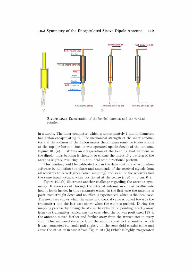
10.3 Symmetry of the Encapsulated Sleeve Dipole Antenna 119
(a) (b)
Figure 10.1: Exaggeration of the bended antenna and the verticalrotation.
in a dipole. The inner conductor, which is approximately 1 mm in diameter,has Teflon encapsulating it. The mechanical strength of the inner conduc-tor and the softness of the Teflon makes the antenna sensitive to deviationsat the top (or bottom since it was operated upside down) of the antenna.Figure 10.1(a) illustrates an exaggeration of the bending that happens inthe dipole. This bending is thought to change the directivity pattern of theantenna slightly, resulting in a non-ideal omnidirectional pattern.
This bending could be calibrated out in the data control and acquisitionsoftware by adjusting the phase and amplitude of the received signals fromall receivers to zero degrees (when mapping) and so all of the receivers hadthe same input voltage, when positioned at the centre (r, φ) = (0 cm, 0).
Figure 10.1(b) illustrates another challenge regarding the antenna sym-metry. It shows a cut through the internal antenna mount as to illustratehow it looks inside, in three separate cases. In the first case the antenna ispositioned straight down and no offset is experienced, which is the ideal case.The next case shows when the semi-rigid coaxial cable is pulled towards thetransmitter and the last case shows when the cable is pushed. During themapping process, by having the slot in the cylinder lid pointing directly awayfrom the transmitter (which was the case when the lid was positioned 135),the antenna moved farther and farther away from the transmitter in everystep. This increased distance from the antenna and to transmitter, whichit was connected to, could pull slightly on the semi-rigid coaxial cable andcause the situation in case 2 from Figure 10.1(b) (which is highly exaggerated
10.4 Position Offset of Inner Cylinder 120
for visual purposes).Case 3 from Figure 10.1(b) could happen when the slot in the lid would
be on exactly the opposite as in case 2, i.e. at 315. Now the internal antennawould get closer to the transmitter and therefore the semi-rigid cable of theinternal antenna could be slightly pushed.
The semi-rigid coaxial cable that was connected to the internal antennais, as the name indicates, rather stiff and did not bend with various po-sitioning of the internal antenna inside the phantom. A super-flex cableconnected the semi-rigid cable to the transmitter (receiver) and provided acertain flexibility when moving the internal antenna around. Even thoughit is much more flexible than the semi-rigid cable, it still needed to maintaincertain phase stability, i.e. one typically does not want the phase to shiftmuch when bending the cable. The super-flex cable has a double shielding toreduce leakage. This could, however, limit the flexibility of the cable whichmakes it not flexible enough to completely eliminate the offset of the internalantenna.
Rubber fittings were placed at the top and at the bottom of the internalantenna mount as is indicated in Figure 10.1(b) to reduce the offset describedabove. Electrical tape was also wrapped around the coaxial cable, at onepoint, to fill up the gap between the coaxial cable and the antenna mountwhich centralizes the antenna even further.
When rotating the lid on top of the outer phantom cylinder, the internalantenna and the semi-rigid coaxial cable did not actually rotate with it,only the internal antenna mount. A compromise had therefore to be madebetween centralizing the antenna and avoiding to completely fix it in theantenna mount.
10.4 Position Offset of Inner Cylinder
The inner cylinder was not completely fixed to the outer cylinder. Thiscaused a slight position offset of the inner cylinder in respect to the outerone. The submerged antenna was mounted on the lid which rotated on thetop of the outer cylinder and did therefore not rotate completely concentricto the inner cylinder. As mentioned before, a doughnut shaped polystyrenewas placed in between the two cylinders to hold their respective positions.Even though the polystyrene held the cylinders in place, there was an offsetof up to 3 mm due to deviations since the polystyrene was cut by hand.Figure 10.2 shows a much exaggerated example of this offset.
This offset would cause the wave, propagating from the submerged an-tenna, to travel faster (due to lower permittivity of fat compared to muscle)and therefore with less phase shift towards perhaps one receiver rather thananother, even though the antenna is e.g. positioned at (r, φ) = (0 cm, 0).This could skew the phase and amplitudes measurements during mapping
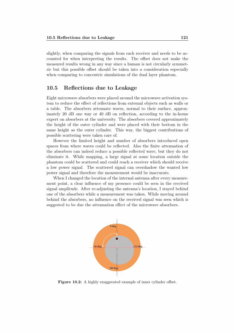
10.5 Reflections due to Leakage 121
slightly, when comparing the signals from each receiver and needs to be ac-counted for when interpreting the results. The offset does not make themeasured results wrong in any way since a human is not circularly symmet-ric but this possible offset should be taken into a consideration especiallywhen comparing to concentric simulations of the dual layer phantom.
10.5 Reflections due to Leakage
Eight microwave absorbers were placed around the microwave activation sys-tem to reduce the effect of reflections from external objects such as walls ora table. The absorbers attenuate waves, normal to their surface, approx-imately 20 dB one way or 40 dB on reflection, according to the in-houseexpert on absorbers at the university. The absorbers covered approximatelythe height of the outer cylinder and were placed with their bottom in thesame height as the outer cylinder. This way, the biggest contributions ofpossible scattering were taken care of.
However the limited height and number of absorbers introduced openspaces from where waves could be reflected. Also the finite attenuation ofthe absorbers can indeed reduce a possible reflected wave, but they do noteliminate it. While mapping, a large signal at some location outside thephantom could be scattered and could reach a receiver which should receivea low power signal. The scattered signal can overshadow the wanted lowpower signal and therefore the measurement would be inaccurate.
When I changed the location of the internal antenna after every measure-ment point, a clear influence of my presence could be seen in the receivedsignal amplitude. After re-adjusting the antenna’s location, I stayed behindone of the absorbers while a measurement was taken. While moving aroundbehind the absorbers, no influence on the received signal was seen which issuggested to be due the attenuation effect of the microwave absorbers.
Figure 10.2: A highly exaggerated example of inner cylinder offset.

122
Chapter 11
Micro-Containers forPharmaceutical Drugs
11.1 Introduction
Conventional pharmaceutical drug delivery, such as oral delivery of therapeu-tics, faces several obstacles. There are problems such as low drug penetrationthrough the gastrointestinal wall, degradation of the active pharmaceuticalcomponents in the stomach and the lack of external control of the actualtime and place of the drug release [2–4]. By externally activating pharma-ceutical drug capsules, e.g. by focusing microwaves into the area of interestand heating up the capsule, as shown in Figure 11.1, the time and place forthe drug release can be pre-determined.
Various techniques have been suggested for external drug activation thatare sensitive to magnetic fields [10], ultrasound [8], light waves [9] and radio-waves below 100 MHz [11] as was presented in Chapter 1. Complex drugdelivery modules including a receiving inductor, control circuitry chip and adrug delivery chip that uses low frequency EM waves for excitation, have alsobeen published in the literature, [12]. These techniques have disadvantagessuch as the inability to focus magnetic fields and low frequency electromag-netic waves, light wave is limited to only surface excitation and a high levelof complexity in the control circuitry.
At microwave frequencies, the possibility of focusing inside human bodiescould become realizable where the high-amplitude areas could be used for thedrug activation. The inherent high losses of biological tissues at microwavefrequencies as shown in previous chapters make it challenging to penetratedeep into tissues with sufficient power levels. It is therefore suggested tohave a very sensitive receiving structure on the drug capsule to absorb asignificant part of the power that is available, in order to use that energy toopen the capsule. A highly resonant structure, the split-ring resonator (SRR)is introduced in an attempt to accomplish this. A resonator is able to induce
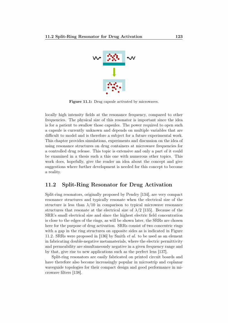
11.2 Split-Ring Resonator for Drug Activation 123
Figure 11.1: Drug capsule activated by microwaves.
locally high intensity fields at the resonance frequency, compared to otherfrequencies. The physical size of this resonator is important since the ideais for a patient to swallow those capsules. The power required to open sucha capsule is currently unknown and depends on multiple variables that aredifficult to model and is therefore a subject for a future experimental work.This chapter provides simulations, experiments and discussion on the idea ofusing resonance structures on drug containers at microwave frequencies fora controlled drug release. This topic is extensive and only a part of it couldbe examined in a thesis such a this one with numerous other topics. Thiswork does, hopefully, give the reader an idea about the concept and givesuggestions where further development is needed for this concept to becomea reality.
11.2 Split-Ring Resonator for Drug Activation
Split-ring resonators, originally proposed by Pendry [134], are very compactresonance structures and typically resonate when the electrical size of thestructure is less than λ/10 in comparison to typical microwave resonancestructures that resonate at the electrical size of λ/2 [135]. Because of theSRR’s small electrical size and since the highest electric field concentrationis close to the edges of the rings, as will be shown later, the SRRs are chosenhere for the purpose of drug activation. SRRs consist of two concentric ringswith a gap in the ring structures on opposite sides as is indicated in Figure11.2. SRRs were proposed in [136] by Smith et al. to be used as an elementin fabricating double-negative metamaterials, where the electric permittivityand permeability are simultaneously negative in a given frequency range andby that, give rise to new applications such as the perfect lens [137].
Split-ring resonators are easily fabricated on printed circuit boards andhave therefore also become increasingly popular in microstrip and coplanarwaveguide topologies for their compact design and good performance in mi-crowave filters [138].
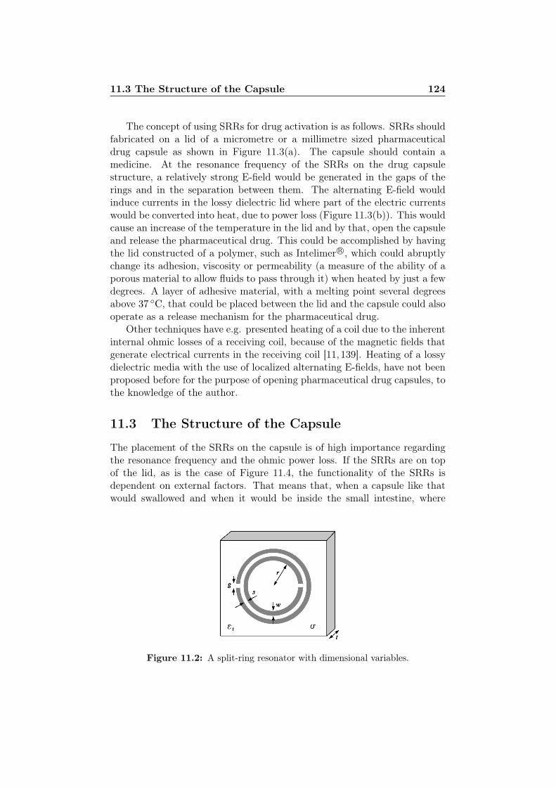
11.3 The Structure of the Capsule 124
The concept of using SRRs for drug activation is as follows. SRRs shouldfabricated on a lid of a micrometre or a millimetre sized pharmaceuticaldrug capsule as shown in Figure 11.3(a). The capsule should contain amedicine. At the resonance frequency of the SRRs on the drug capsulestructure, a relatively strong E-field would be generated in the gaps of therings and in the separation between them. The alternating E-field wouldinduce currents in the lossy dielectric lid where part of the electric currentswould be converted into heat, due to power loss (Figure 11.3(b)). This wouldcause an increase of the temperature in the lid and by that, open the capsuleand release the pharmaceutical drug. This could be accomplished by havingthe lid constructed of a polymer, such as Intelimer R©, which could abruptlychange its adhesion, viscosity or permeability (a measure of the ability of aporous material to allow fluids to pass through it) when heated by just a fewdegrees. A layer of adhesive material, with a melting point several degreesabove 37 C, that could be placed between the lid and the capsule could alsooperate as a release mechanism for the pharmaceutical drug.
Other techniques have e.g. presented heating of a coil due to the inherentinternal ohmic losses of a receiving coil, because of the magnetic fields thatgenerate electrical currents in the receiving coil [11, 139]. Heating of a lossydielectric media with the use of localized alternating E-fields, have not beenproposed before for the purpose of opening pharmaceutical drug capsules, tothe knowledge of the author.
11.3 The Structure of the Capsule
The placement of the SRRs on the capsule is of high importance regardingthe resonance frequency and the ohmic power loss. If the SRRs are on topof the lid, as is the case of Figure 11.4, the functionality of the SRRs isdependent on external factors. That means that, when a capsule like thatwould swallowed and when it would be inside the small intestine, where
Figure 11.2: A split-ring resonator with dimensional variables.
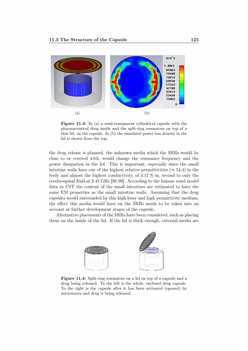
11.3 The Structure of the Capsule 125
(a) (b)
Figure 11.3: In (a) a semi-transparent cylindrical capsule with thepharmaceutical drug inside and the split-ring resonators on top of athin lid, on the capsule. In (b) the simulated power loss density in thelid is shown from the top.
the drug release is planned, the unknown media which the SRRs would beclose to or covered with, would change the resonance frequency and thepower dissipation in the lid. This is important, especially since the smallintestine walls have one of the highest relative permittivities (≈ 54.4) in thebody and almost the highest conductivity, of 3.17 S/m, second to only thecerebrospinal fluid at 2.45 GHz [98,99]. According to the human voxel modeldata in CST the content of the small intestines are estimated to have thesame EM properties as the small intestine walls. Assuming that the drugcapsules would surrounded by this high lossy and high permittivity medium,the effect this media would have on the SRRs needs to be taken into anaccount at further development stages of the capsule.
Alternative placements of the SRRs have been considered, such as placingthem on the inside of the lid. If the lid is thick enough, external media are
Figure 11.4: Split-ring resonators on a lid on top of a capsule and adrug being released. To the left is the whole, enclosed drug capsule.To the right is the capsule after it has been activated (opened) bymicrowaves and drug is being released.
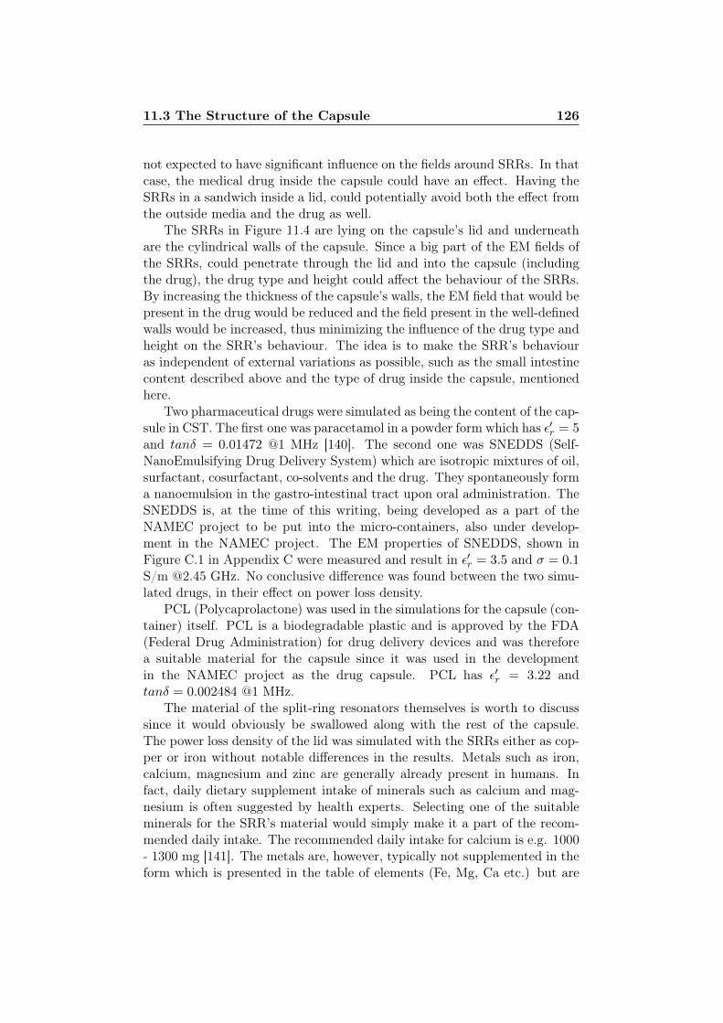
11.3 The Structure of the Capsule 126
not expected to have significant influence on the fields around SRRs. In thatcase, the medical drug inside the capsule could have an effect. Having theSRRs in a sandwich inside a lid, could potentially avoid both the effect fromthe outside media and the drug as well.
The SRRs in Figure 11.4 are lying on the capsule’s lid and underneathare the cylindrical walls of the capsule. Since a big part of the EM fields ofthe SRRs, could penetrate through the lid and into the capsule (includingthe drug), the drug type and height could affect the behaviour of the SRRs.By increasing the thickness of the capsule’s walls, the EM field that would bepresent in the drug would be reduced and the field present in the well-definedwalls would be increased, thus minimizing the influence of the drug type andheight on the SRR’s behaviour. The idea is to make the SRR’s behaviouras independent of external variations as possible, such as the small intestinecontent described above and the type of drug inside the capsule, mentionedhere.
Two pharmaceutical drugs were simulated as being the content of the cap-sule in CST. The first one was paracetamol in a powder form which has ε′r = 5and tanδ = 0.01472 @1 MHz [140]. The second one was SNEDDS (Self-NanoEmulsifying Drug Delivery System) which are isotropic mixtures of oil,surfactant, cosurfactant, co-solvents and the drug. They spontaneously forma nanoemulsion in the gastro-intestinal tract upon oral administration. TheSNEDDS is, at the time of this writing, being developed as a part of theNAMEC project to be put into the micro-containers, also under develop-ment in the NAMEC project. The EM properties of SNEDDS, shown inFigure C.1 in Appendix C were measured and result in ε′r = 3.5 and σ = 0.1S/m @2.45 GHz. No conclusive difference was found between the two simu-lated drugs, in their effect on power loss density.
PCL (Polycaprolactone) was used in the simulations for the capsule (con-tainer) itself. PCL is a biodegradable plastic and is approved by the FDA(Federal Drug Administration) for drug delivery devices and was thereforea suitable material for the capsule since it was used in the developmentin the NAMEC project as the drug capsule. PCL has ε′r = 3.22 andtanδ = 0.002484 @1 MHz.
The material of the split-ring resonators themselves is worth to discusssince it would obviously be swallowed along with the rest of the capsule.The power loss density of the lid was simulated with the SRRs either as cop-per or iron without notable differences in the results. Metals such as iron,calcium, magnesium and zinc are generally already present in humans. Infact, daily dietary supplement intake of minerals such as calcium and mag-nesium is often suggested by health experts. Selecting one of the suitableminerals for the SRR’s material would simply make it a part of the recom-mended daily intake. The recommended daily intake for calcium is e.g. 1000- 1300 mg [141]. The metals are, however, typically not supplemented in theform which is presented in the table of elements (Fe, Mg, Ca etc.) but are
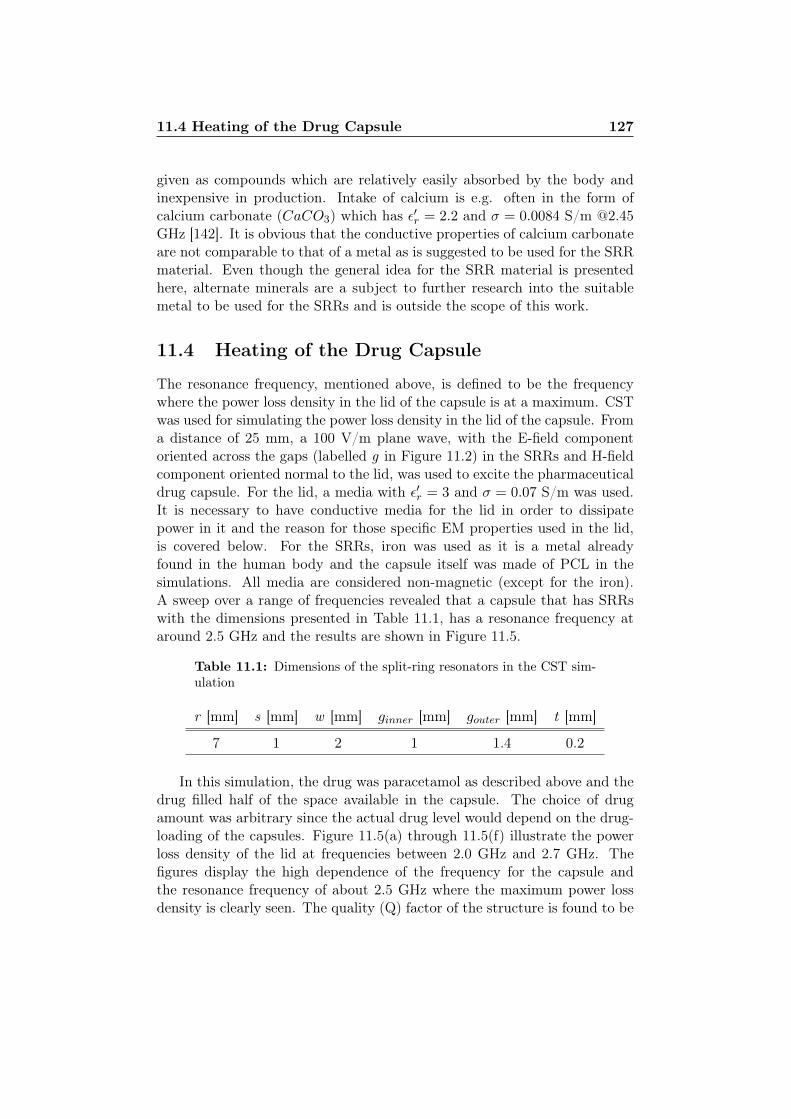
11.4 Heating of the Drug Capsule 127
given as compounds which are relatively easily absorbed by the body andinexpensive in production. Intake of calcium is e.g. often in the form ofcalcium carbonate (CaCO3) which has ε′r = 2.2 and σ = 0.0084 S/m @2.45GHz [142]. It is obvious that the conductive properties of calcium carbonateare not comparable to that of a metal as is suggested to be used for the SRRmaterial. Even though the general idea for the SRR material is presentedhere, alternate minerals are a subject to further research into the suitablemetal to be used for the SRRs and is outside the scope of this work.
11.4 Heating of the Drug Capsule
The resonance frequency, mentioned above, is defined to be the frequencywhere the power loss density in the lid of the capsule is at a maximum. CSTwas used for simulating the power loss density in the lid of the capsule. Froma distance of 25 mm, a 100 V/m plane wave, with the E-field componentoriented across the gaps (labelled g in Figure 11.2) in the SRRs and H-fieldcomponent oriented normal to the lid, was used to excite the pharmaceuticaldrug capsule. For the lid, a media with ε′r = 3 and σ = 0.07 S/m was used.It is necessary to have conductive media for the lid in order to dissipatepower in it and the reason for those specific EM properties used in the lid,is covered below. For the SRRs, iron was used as it is a metal alreadyfound in the human body and the capsule itself was made of PCL in thesimulations. All media are considered non-magnetic (except for the iron).A sweep over a range of frequencies revealed that a capsule that has SRRswith the dimensions presented in Table 11.1, has a resonance frequency ataround 2.5 GHz and the results are shown in Figure 11.5.
Table 11.1: Dimensions of the split-ring resonators in the CST sim-ulation
r [mm] s [mm] w [mm] ginner [mm] gouter [mm] t [mm]
7 1 2 1 1.4 0.2
In this simulation, the drug was paracetamol as described above and thedrug filled half of the space available in the capsule. The choice of drugamount was arbitrary since the actual drug level would depend on the drug-loading of the capsules. Figure 11.5(a) through 11.5(f) illustrate the powerloss density of the lid at frequencies between 2.0 GHz and 2.7 GHz. Thefigures display the high dependence of the frequency for the capsule andthe resonance frequency of about 2.5 GHz where the maximum power lossdensity is clearly seen. The quality (Q) factor of the structure is found to be
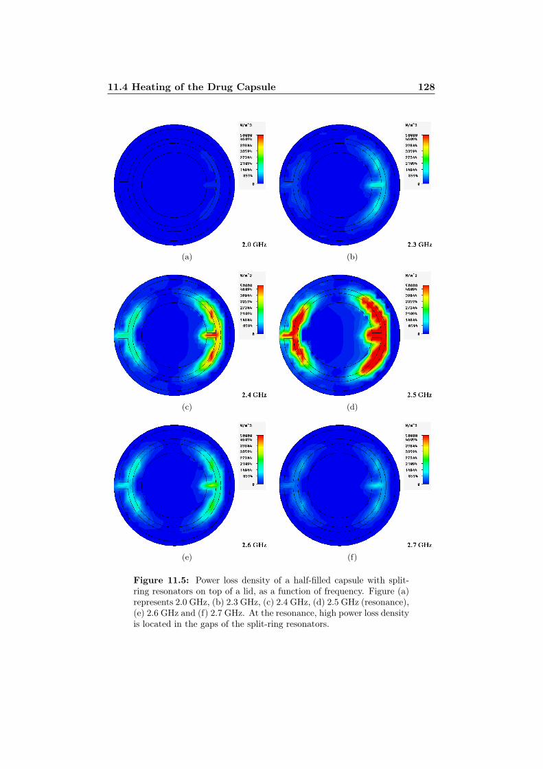
11.4 Heating of the Drug Capsule 128
(a) (b)
(c) (d)
(e) (f)
Figure 11.5: Power loss density of a half-filled capsule with split-ring resonators on top of a lid, as a function of frequency. Figure (a)represents 2.0 GHz, (b) 2.3 GHz, (c) 2.4 GHz, (d) 2.5 GHz (resonance),(e) 2.6 GHz and (f) 2.7 GHz. At the resonance, high power loss densityis located in the gaps of the split-ring resonators.
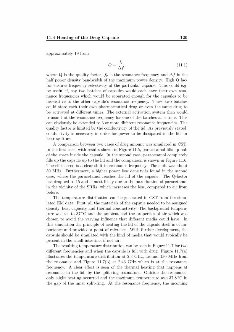
11.4 Heating of the Drug Capsule 129
approximately 19 from
Q =fr∆f
, (11.1)
where Q is the quality factor, fr is the resonance frequency and ∆f is thehalf power density bandwidth of the maximum power density. High Q fac-tor ensures frequency selectivity of the particular capsule. This could e.g.be useful if, say two batches of capsules would each have their own reso-nance frequencies which would be separated enough for the capsules to beinsensitive to the other capsule’s resonance frequency. These two batchescould store each their own pharmaceutical drug or even the same drug tobe activated at different times. The external activation system then wouldtransmit at the resonance frequency for one of the batches at a time. Thiscan obviously be extended to 3 or more different resonance frequencies. Thequality factor is limited by the conductivity of the lid. As previously stated,conductivity is necessary in order for power to be dissipated in the lid forheating it up.
A comparison between two cases of drug amount was simulated in CST.In the first case, with results shown in Figure 11.5, paracetamol fills up halfof the space inside the capsule. In the second case, paracetamol completelyfills up the capsule up to the lid and the comparison is shown in Figure 11.6.The effect seen is a clear shift in resonance frequency. The shift was about50 MHz. Furthermore, a higher power loss density is found in the secondcase, where the paracetamol reaches the lid of the capsule. The Q-factorhas dropped to 15 and is most likely due to the introduction of paracetamolin the vicinity of the SRRs, which increases the loss, compared to air frombefore.
The temperature distribution can be generated in CST from the simu-lated EM data. First, all the materials of the capsule needed to be assigneddensity, heat capacity and thermal conductivity. The background tempera-ture was set to 37 C and the ambient had the properties of air which waschosen to avoid the varying influence that different media could have. Inthis simulation the principle of heating the lid of the capsule itself is of im-portance and provided a point of reference. With further development, thecapsule should be simulated with the kind of media that would typically bepresent in the small intestine, if not air.
The resulting temperature distribution can be seen in Figure 11.7 for twodifferent frequencies and when the capsule is full with drug. Figure 11.7(a)illustrates the temperature distribution at 2.3 GHz, around 130 MHz fromthe resonance and Figure 11.7(b) at 2.43 GHz which is at the resonancefrequency. A clear effect is seen of the thermal heating that happens atresonance in the lid, by the split-ring resonators. Outside the resonance,only slight heating occurred and the maximum temperature was 37.8 C inthe gap of the inner split-ring. At the resonance frequency, the incoming
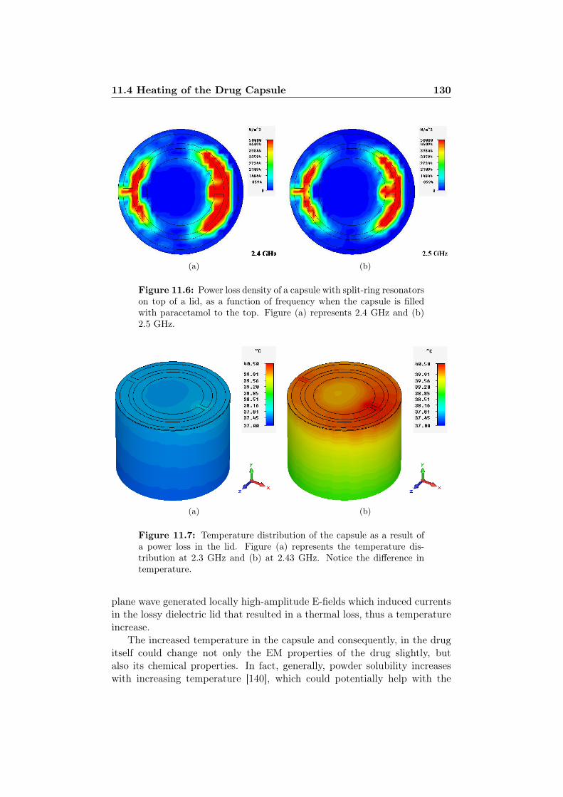
11.4 Heating of the Drug Capsule 130
(a) (b)
Figure 11.6: Power loss density of a capsule with split-ring resonatorson top of a lid, as a function of frequency when the capsule is filledwith paracetamol to the top. Figure (a) represents 2.4 GHz and (b)2.5 GHz.
(a) (b)
Figure 11.7: Temperature distribution of the capsule as a result ofa power loss in the lid. Figure (a) represents the temperature dis-tribution at 2.3 GHz and (b) at 2.43 GHz. Notice the difference intemperature.
plane wave generated locally high-amplitude E-fields which induced currentsin the lossy dielectric lid that resulted in a thermal loss, thus a temperatureincrease.
The increased temperature in the capsule and consequently, in the drugitself could change not only the EM properties of the drug slightly, butalso its chemical properties. In fact, generally, powder solubility increaseswith increasing temperature [140], which could potentially help with the
11.5 Optimizing Power Dissipation in the Lid 131
absorption efficiency of the drug in the body.Multiple split-ring resonators, split-rings on the side of the capsule, a
rectangular capsule with split-rings on each side and four concentric ringseach with their gap at a 90 offset are among the structural possibilities toprovide alternate heating spot pattern and different method of drug release,if required.
The diameter of the pharmaceutical capsule presented in these simula-tions was 26 mm which is relatively large for a capsule to be swallowed andwould need to be reduced by at least one half. The SRRs have not beenoptimized in respect to their physical size in any regards. A media for thelid with higher relative permittivity could be the first step in the size re-duction process. By having the SRRs inside the lid or on the other side ofthe lid, they would be surrounded, effectively, by a media of higher relativepermittivity and therefore their size would be reduced, for the same reso-nance frequency. I believe that the size and the arrangement of the SRRsand therefore the capsule can be reduced significantly, if optimized.
11.5 Optimizing Power Dissipation in the Lid
In general, substrates which are too conductive tend to short-circuit theSRRs which are fabricated on the substrate and kill off any resonance inthe rings. On the other hand, substrates that have very low conductivity,dissipate very little power.
Rogers 4003 R©, for example, is a low-loss substrate with σ = 0.001 S/mand ε′r = 3.55 @2.5 GHz and SRRs that are fabricated on such a substrate,behave as Hi-Q resonators, as is often the aspired property for filters, anddo therefore not dissipate notable power. Most substrates that are usedin printed circuit technology are relatively low-loss which means that lossysubstrates that can be used in conventional photolithography processes canbe difficult to find for the purpose of dissipating power.
Simulations of the optimal conductivity for a given relative permittivitywere performed in CST in order to provide the optimal parameters for max-imum temperature in the lid. Same as before, at a distance of 25 mm, a 100V/m plane wave, with the E-field component oriented across the gaps in theSRRs and H-field component oriented normal to the lid, was used to excitethe pharmaceutical drug capsule. All parameters were kept constant exceptfor the relative permittivity and the conductivity. The maximum tempera-ture point of the substrate at each combination of ε′r and σ at the resonancefrequency was taken. The result is shown in Figure 11.8. For a wide rangeof conductivities (Figure 11.8(a)) the maximum temperature was found tobe 41.5 C for a substrate with ε′r = 3 and σ = 0.07 S/m. The power lossdensity for the case of maximum dissipation is indicated in Figure 11.3(b)where it is illustrated that most of the lost power would be dissipated in the
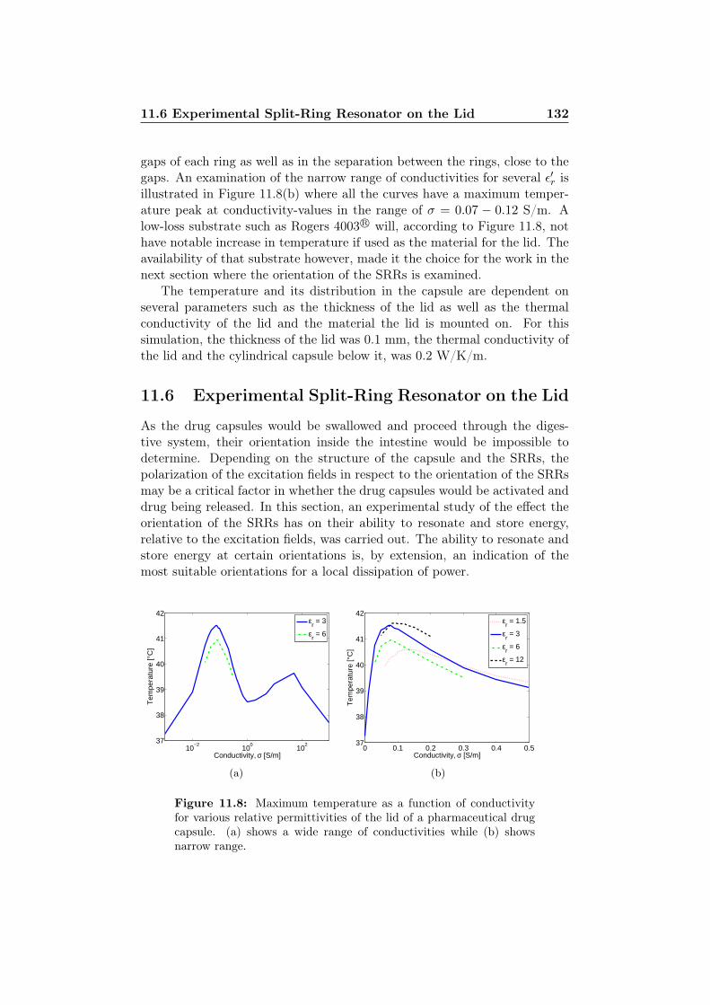
11.6 Experimental Split-Ring Resonator on the Lid 132
gaps of each ring as well as in the separation between the rings, close to thegaps. An examination of the narrow range of conductivities for several ε′r isillustrated in Figure 11.8(b) where all the curves have a maximum temper-ature peak at conductivity-values in the range of σ = 0.07 − 0.12 S/m. Alow-loss substrate such as Rogers 4003 R© will, according to Figure 11.8, nothave notable increase in temperature if used as the material for the lid. Theavailability of that substrate however, made it the choice for the work in thenext section where the orientation of the SRRs is examined.
The temperature and its distribution in the capsule are dependent onseveral parameters such as the thickness of the lid as well as the thermalconductivity of the lid and the material the lid is mounted on. For thissimulation, the thickness of the lid was 0.1 mm, the thermal conductivity ofthe lid and the cylindrical capsule below it, was 0.2 W/K/m.
11.6 Experimental Split-Ring Resonator on the Lid
As the drug capsules would be swallowed and proceed through the diges-tive system, their orientation inside the intestine would be impossible todetermine. Depending on the structure of the capsule and the SRRs, thepolarization of the excitation fields in respect to the orientation of the SRRsmay be a critical factor in whether the drug capsules would be activated anddrug being released. In this section, an experimental study of the effect theorientation of the SRRs has on their ability to resonate and store energy,relative to the excitation fields, was carried out. The ability to resonate andstore energy at certain orientations is, by extension, an indication of themost suitable orientations for a local dissipation of power.
10−2
100
102
37
38
39
40
41
42
Conductivity, σ [S/m]
Tem
pera
ture
[°C
]
εr = 3
εr = 6
(a)
0 0.1 0.2 0.3 0.4 0.537
38
39
40
41
42
Conductivity, σ [S/m]
Tem
pera
ture
[°C
]
εr = 1.5
εr = 3
εr = 6
εr = 12
(b)
Figure 11.8: Maximum temperature as a function of conductivityfor various relative permittivities of the lid of a pharmaceutical drugcapsule. (a) shows a wide range of conductivities while (b) showsnarrow range.
11.6 Experimental Split-Ring Resonator on the Lid 133
11.6.1 Fabrication
Split-ring resonators on top of a 1.5 mm thick Rogers 4003 R© substrate werefabricated for the experimental study. Each of the SRRs were fabricated ona circular disc with the diameter of 15 mm that functions as an enlarged lidfor a drug capsule. The dimensions of the SRRs are shown in Table 11.2 andtheir notations are referred to Figure 11.2. As mentioned before, the relativepermittivity and conductivity at 2.5 GHz are εr = 3.55 and σ = 0.001 S/m,respectively.
Table 11.2: Dimensions of the split-ring resonators in the experi-mental study.
r [mm] s [mm] w [mm] g [mm] t [mm]
5.1 0.3 0.3 0.2 1.5
11.6.2 Excitation
Having an external antenna array and focusing microwaves inside the humanbody from a far-field distance, we assume, in general, a propagating trans-verse electromagnetic (TEM) mode inside the body. This field would excitethe pharmaceutical drug capsule and especially the split-ring resonators ontop of the lid until the drug would be released. To approximate such aTEM excitation, a coplanar waveguide (CPW) structure was fabricated andis shown in Figure 11.9. Waves on a CPW have typically a quasi-TEM modesince part of the wave is located in the substrate while the other part is lo-cated in air. The CPW is approximately a 50 Ω tapered transmission linewith a 15 mm gap between the centre conductor and the ground referencesin the middle of the CPW structure. The large gap makes it possible to fitthe lids. This was accomplished by drilling a hole in the substrate in themiddle of the gap of the CPW and leaving room for placing the cylindricallid structures. In the plane of the CPW structure, the E-field component wasoriented across the gap where the SRRs are placed, the H-field componentwas oriented normal to the CPW structure and the direction of propagation,k, was normal to the E-H plane as is indicated in Figure 11.9.
11.6.3 Measurements
Measurements on six different orientations of the SRRs were performed. Theorientations are indicated in Figure 11.10 and are relative to the orientationof the quasi-TEM wave that was propagating in the CPW plane in Fig. 11.9.Each subfigure notation in Fig. 11.10 will be referred to as a case, e.g. theorientation in Figure 11.10(e) is referred to as case (e) and so on. For every
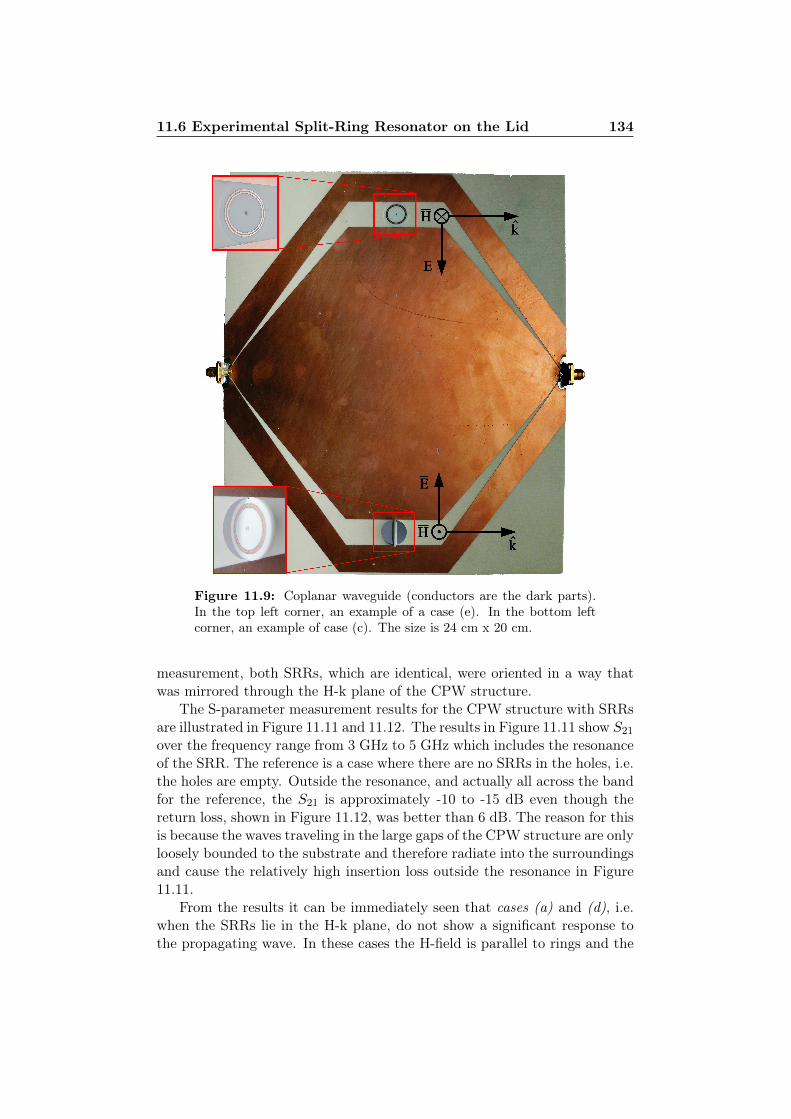
11.6 Experimental Split-Ring Resonator on the Lid 134
Figure 11.9: Coplanar waveguide (conductors are the dark parts).In the top left corner, an example of a case (e). In the bottom leftcorner, an example of case (c). The size is 24 cm x 20 cm.
measurement, both SRRs, which are identical, were oriented in a way thatwas mirrored through the H-k plane of the CPW structure.
The S-parameter measurement results for the CPW structure with SRRsare illustrated in Figure 11.11 and 11.12. The results in Figure 11.11 show S21over the frequency range from 3 GHz to 5 GHz which includes the resonanceof the SRR. The reference is a case where there are no SRRs in the holes, i.e.the holes are empty. Outside the resonance, and actually all across the bandfor the reference, the S21 is approximately -10 to -15 dB even though thereturn loss, shown in Figure 11.12, was better than 6 dB. The reason for thisis because the waves traveling in the large gaps of the CPW structure are onlyloosely bounded to the substrate and therefore radiate into the surroundingsand cause the relatively high insertion loss outside the resonance in Figure11.11.
From the results it can be immediately seen that cases (a) and (d), i.e.when the SRRs lie in the H-k plane, do not show a significant response tothe propagating wave. In these cases the H-field is parallel to rings and the
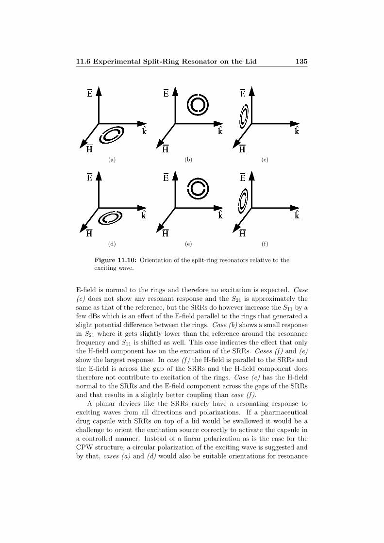
11.6 Experimental Split-Ring Resonator on the Lid 135
(a) (b) (c)
(d) (e) (f)
Figure 11.10: Orientation of the split-ring resonators relative to theexciting wave.
E-field is normal to the rings and therefore no excitation is expected. Case(c) does not show any resonant response and the S21 is approximately thesame as that of the reference, but the SRRs do however increase the S11 by afew dBs which is an effect of the E-field parallel to the rings that generated aslight potential difference between the rings. Case (b) shows a small responsein S21 where it gets slightly lower than the reference around the resonancefrequency and S11 is shifted as well. This case indicates the effect that onlythe H-field component has on the excitation of the SRRs. Cases (f) and (e)show the largest response. In case (f) the H-field is parallel to the SRRs andthe E-field is across the gap of the SRRs and the H-field component doestherefore not contribute to excitation of the rings. Case (e) has the H-fieldnormal to the SRRs and the E-field component across the gaps of the SRRsand that results in a slightly better coupling than case (f).
A planar devices like the SRRs rarely have a resonating response toexciting waves from all directions and polarizations. If a pharmaceuticaldrug capsule with SRRs on top of a lid would be swallowed it would be achallenge to orient the excitation source correctly to activate the capsule ina controlled manner. Instead of a linear polarization as is the case for theCPW structure, a circular polarization of the exciting wave is suggested andby that, cases (a) and (d) would also be suitable orientations for resonance
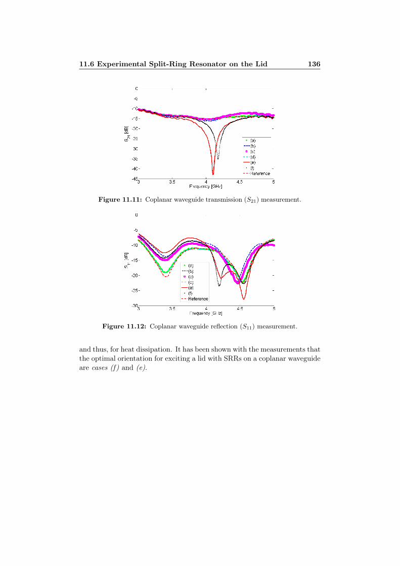
11.6 Experimental Split-Ring Resonator on the Lid 136
Figure 11.11: Coplanar waveguide transmission (S21) measurement.
Figure 11.12: Coplanar waveguide reflection (S11) measurement.
and thus, for heat dissipation. It has been shown with the measurements thatthe optimal orientation for exciting a lid with SRRs on a coplanar waveguideare cases (f) and (e).
137
Chapter 12
Conclusion
In this PhD thesis, a method of externally activating and releasing phar-maceutical drugs inside the human body with the use of microwaves, wasinvestigated. Current limitations in external control of the specific locationand the time of a drug release inside the human body formed the motiva-tion for this study. A two-sided solution to this problem was considered.First, a microwave activation system, consisting of four transmitting sourcesthat radiate electromagnetic waves, at a human torso. Secondly, a speciallydesigned micro-container for pharmaceutical drugs with sensitive receivingstructure to effectively utilize the received power for releasing the drug.
In the beginning of the thesis, electromagnetic properties of biologicaltissues were described and especially the wave interaction at a interface be-tween air and fat at an oblique incident angle, which gave rise to possibil-ities of optimum power transfer under a certain condition. If the angle ofincidence is set to be the Brewster angle, maximum power transfer could po-tentially be accomplished into a lossy media such as a skin or fat layer. Atoblique incidence angles, the power loss of the transmitted wave in the lossymedia is only dependent on the distance the wave travels in the directionnormal to the interface of the lossy media. The combination of utilizing theBrewster angle along with the fact that a wave is only attenuated in the nor-mal direction of an interface, gives the possibility of maximizing the powertransfer of a transmitted wave to a pre-determined point inside a lossy tissue.
For representing a human torso, a simple dual-layered cylindrical phan-tom was proposed. The phantom consists of two concentric plastic cylinders.The inner cylinder holds the muscle tissue mimicking media which, as thename indicates, emulates the electromagnetic properties of muscle tissue atthe operating frequency of 2.45 GHz whereas the outer cylinder holds thefat mimicking media. In order to be able to move a measuring or a trans-mitting antenna around freely, inside the phantom, a low-viscous optically
138
transparent muscle tissue mimicking media was developed and the resultingrecipe is 28% Diethylene Glycol Butyl Ether and 72% de-ionized water. Animproved liquid whose properties are within 1% from the reference valuesfor muscle tissue at 2.45 GHz, a recipe of 5% Triton X-100, 23% DiethyleneGlycol Butyl Ether and 72% de-ionized water was furthermore produced.
The microwave activation system was developed on the basis of being anunobtrusive system, i.e. without disturbing the prospective patients. To thisend, four external antennas were designed to radiate in the far-field, at thetorso phantom along with four microwave transmitters and four receivers.The operation of the system was two-fold. First, a mapping of the torsophantom was performed. This required an antenna, submerged in the mus-cle tissue mimicking medium to transmit from within the phantom and theexternal antennas were connected to receivers. The transmitting antennawas systematically moved around inside the phantom while phase and am-plitude measurements were acquired. The measurement results revealed thatcreeping waves were travelling along the curvature of the phantom, reachingthe receiver furthest away from the transmitting source. If the source was ata certain offset from the centre of the phantom, these creeping waves over-shadowed the contribution of the wave travelling along the direct path fromthe source to the receiver furthest away, due to the high attenuation in themuscle tissue mimicking media.
The measurements also gave an indication of standing waves between thetransmitting source and the layers of the phantom as well as the externalantennas. This was especially evident at locations inside the phantom wherethe transmitting source was close to the edge of the phantom.
The measurement results presented in the mapping process disclosed thewave behaviour in the cylindrical phantom. In agreement with Lorentz’sreciprocity theorem, these results predicted the behaviour of the second op-eration, i.e. the focusing.
In the focusing operation, four external transmitters radiated microwavesat the torso phantom from a distance of 65 cm. Two receivers were used.One receiver was connected to the antenna submerged in the muscle tissuemimicking media for the purpose of measuring the amplitude and phaseof the received signal. The other receiver was directly connected to bothfrequency synthesizers and provided a constant phase reference for calibra-tion purposes. The measuring submerged antenna was systematically movedaround in the phantom and the amplitudes were measured to uncover thefocus point, if any.
Already predicted by the mapping process, it was not possible to focusat 4 cm offset from the centre of the phantom and at larger offsets. Thisis believed to be due to the contribution of the creeping waves which arealso thought to be present if radiating at a human. At 3 cm offset andbelow, focusing was accomplished. The focusing resulted in a point of alocal maximum with a distance of approximately 2 cm to a neighbouring
139
point of similar amplitude.Predicted by simulations, a part of the waves that a source radiates at a
phantom from one side, crawls along the surface of the phantom, from bothsides, where they are added in phase on the opposite side of the phantom.These added creeping waves then radiate partly inwards into the phantomwhere their power is combined with power radiated from other sources. Anexperiment was performed that verified the presence of creeping waves. Alayered microwave absorber was placed in front of and behind the phantom,relative to a single transmitting source. The received amplitude at the loca-tion of the internal antenna, which was offset 8 cm from the centre, revealeda much lower amplitude when the absorber was behind the phantom. Theseunintuitive results suggest that the absorber attenuates the creeping wavesthat crawl around the phantom and previously radiated inwards.
Due to the high losses in muscle tissue mimicking media and the large sizeof the torso phantom, the received signal strength in the phantom were inthe order of pW when radiated with approximately hundred mW. The phan-tom’s dimensions are considerably pessimistic regarding the muscle thicknesswhich explains to a large degree, the high attenuation of the signals trav-elling through the phantom. The high attenuation factor of muscle tissueat 2.45 GHz is also the reason for the low received power, along with theinherent path loss of operating the system in the far-field. A lower operatingfrequency, of around 1 GHz is suggested for a compromise between increasedsize of the radiators and the improved penetration into the body. This, how-ever, increases the challenge of developing resonators for the pharmaceuticaldrug capsule which are sufficiently small. An increased number of radiatorsis also suggested for higher intensity focus point. By placing the radiatorscloser to the target, e.g. at the far-field limit, the effects of path loss can bereduced.
A micro-container with split-ring resonators (SRRs) on top of its lid isproposed to be externally activated in order to release a pharmaceutical druginside the body. The split-ring resonator’s resonance frequency was tunedby CST simulation of the container (capsule). At the resonance frequencyof the SRRs the external electromagnetic waves excited the SRRs whichconcentrated high-amplitude electric fields (E-fields) in the gap of the ringsand their separation. These high-amplitude fields induced currents in thelossy dielectric substrate that the lid is required to be made of. Too lowelectric conductivity of the lid and little power would be dissipated in thelid and too high conductivity would short-circuit the SRRs. The optimalconductivity of the dielectric media which the lid is made of was found withsimulations to be between 0.07 and 0.12 S/m. The induced currents in thelid resulted in a ohmic power loss, thus the temperature of the lid increased.This increased temperature could be used to melt a type of plastic that has amelting point between 37 and 42 C or even an adhesive medium that holds
140
the lid onto the capsule until activated.An experimental setup to find the most optimal orientation of the cap-
sule’s lid was made. Low-loss Rogers 4003 substrate was used as the liddielectric and SRRs were fabricated on top of it. Together, they representedan enlarged lid. A 50 Ω co-planar transmission line with holes in its gaps wasused to place the enlarged lids. In the gap of a co-planar line, quasi-TEM(transverse electromagnetic) fields can exist, approximating pure TEM fieldswhich would be used for exciting the drug capsules. The two most effectiveorientations of the SRRs are predicted to be when the E-field component isoriented across the gap of the SRRs, in the plane of the SRRs. The optimalorientation is when additionally the magnetic field component is normal tothe plane of the SRRs.
The power required for heating up the capsule’s lid seems to be orders ofmagnitude higher than is available from the current experimental microwavesetup at locations deep inside the human torso phantom. It does thereforenot immediately seem possible to use the current system for releasing med-ical drugs externally from the body phantom. That being said, the humantorso phantom is simple and presents a very pessimistic model for a humantorso which results in lower power levels than otherwise would probably beavailable. An effort should also be made into minimizing the size of the SRRsalong with maximizing the dissipated power in the capsule’s lid since thiswork only presents the principle of the concept’s operation and optimizationhas yet to be performed.
REFERENCES 141
References
[1] Qiuping Gu, Charles F. Dillon, and Vicki L. Burt. Prescription druguse continues to increase: U.s. prescription drug data for 2007-2008.NCHS Data Brief, 42:1–8, 2010.
[2] Kristy M. Ainslie, Rachel D. Lowe, Tristan T. Beaudette, Lamar Petty,Eric M. Bachelder, and Tejal A. Desai. Microfabricated devices for en-chanced bioadhesive drug delivery: Attachement to and small-moleculerelease trhough a cell monolayer under flow. Small, 24:2857–2863, 2009.
[3] Colin W. Pouton. Formulation of poorly water-soluble drugs for oraladministration: Physicochemical and physiological issues and the lipidformulation classification system. European Journal of PharmaceuticalSciences, 29:278–287, 2006.
[4] Sanjay B. Bari, Bharati R. Kadam, Yogini S. Jaiswal, and Atul A.Shirkhedkar. Impurity profile: Significance in active pharmaceuticalingredient. Eurasian Journal of Analytical Chemistry, 2:32–53, 2007.
[5] Anja Boisen. Naanomechanical sensors and actuators, fundamentalsand new direction (namec) - a vkr center of excellence. NAMECProject proposal to the VKR Foundation.
[6] David R. Friend. Drug delivery to the small intestine. Current Gas-troenterology Reports, 6:371–376, 2004.
[7] Nazmul Akunjee and Muhammed Akunjee. The Easy Guide to OSCEsfor Final Year Medical Students. Radcliffe Publishing Ltd., 2007.
[8] Holger Grull and Sander Langereis. Hyperthermia-triggered drug de-livery from temperature-sensitive liposomes using mri-guided high in-tensity focused ultrasound. Journal of Controlled Release, 161:317–327,2012.
[9] Cornelius Diamond and Scott Arouh. Light-activated drug deliverymethod and device. Patent, 2003. US 2003/0191458 A1.
[10] Jean Brault. Magnetic apparatus used for drug delivery. Patent, 2011.WO2011113140 (A1).
REFERENCES 142
[11] Somayyeh Rahimi, Elie H. Sarraf, Gregory K. Wong, and Kenichi Taka-hata. Implantable drug delivery device using frequency-controlled wire-less hydrogel microvalves. Biomedical Microdevices, 13:267–277, 2011.
[12] S. Smith, T.B. Tang, J.G. Terry, J.T.M. Stevenson, B.W. Flynn,H.M. Reekie, A.F. Murray, A.M. gundlach, D. Renshaw, B. Dhillon,A. Ohtori, Y. Inoue, and A.J. Walton. Development of a miniaturiseddrug delivery system with wireless power transfer and communication.IET Nanobiotechnology, 1:80–86, 2007.
[13] Gentei Sato, Chokichiro Shibata, Shuichi Sekimukai, Hiroshi Wak-abayashi, Kaoru Mitsuka, and Kenjiro Giga. Phase-controlled circulararray heating equipment for deep-seated tumors: Preliminary experi-ments. IEEE Transactions on Microwave Theory and Techniques, 34:520–525, 1986.
[14] A.J. Fenn and G.A. King. Adaptive radiofrequency hyperthermia-phased array system for improved cancer therapy: phantom targetmeasurements. International Journal of Hyperthermia, 10:189–208,1994.
[15] Paul F. Turner. Hyperthermia and inhomogeneous tissue effects usingan annular phased array. IEEE Transactions on Microwave Theoryand Techniques, 32:874–882, 1984.
[16] Liyong Wu, Robert J. McGough, Omar Ali Arabe, and Thaddeus V.Samulski. An rf phased array applicator designed for hyperthermiabreast cancer treatments. Physics in Medicine and Biology, 51:1–20,2006.
[17] M. Seebass, R. Beck, J. Gellermann, J. Nadobny, and P. Wust. Electro-magnetic phased arrays for regional hyperthermia: optimal frequencyand antenna arrangement. International Journal of Hyperthermia, 17:321–336, 2001.
[18] Margarethus M. Paulides, Jurriaan F. Bakker, Adrianus P. M.Zwamborn, and Gerard C. Van Rhoon. A head and neck hyperthermiaapplicator: Theoretical antenna array design. International Journal ofHyperthermia, 23:59–67, 2007.
[19] J.F. Bakker, M.M. Paulides, A.H. Westra, H.Schippers, and G.C. VanRhoon. Design and test of a 434 mhz multi-channel amplifier sys-tem for targeted hyperthermia applicators. International Journal ofHyperthermia, 26:158–170, 2010.
[20] Masahiro Hiraoka, Michihide Mitsumori, Naotoshi Hiroi, Shinji Ohno,Yoshiaki Tanaka, Youji Kotsuka, and Keizo Sugimachi. Development

REFERENCES 143
of rf and microwave heating equipment and clinical applications tocancer treatment in japan. IEEE Transactions on Microwave Theoryand Techniques, 48:1789–1799, 2000.
[21] Yong-Gang Gu and OM P. Gandhi. Phased-dipole applicators for torsoheating in electromagnetic hyperthermia. IEEE Transactions on Mi-crowave Theory and Techniques, 32:645–647, 1984.
[22] M.M. Paulides, J.F. Bakker, E. Neufeld, J. Van Der Zee, P.P. Jansen,P.C. Levendag, and G.C. Van Rhoon. The hypercollar: A novel appli-cator for hyperthermia in the head and neck. International Journal ofHyperthermia, 23:567–576, 2007.
[23] S. Jacobsen. Reduction of hot spots in hyperthermia by means ofbroadband energy transmission. Electronics Letters, 34:1901–1902,1998.
[24] C.K. Chou, J.A. McDougall, K.W. Chan, and K.H. Luk. Effects of fatthickness on heating patterns of the microwave applicator ma-151 at631 and 915 mhz. International Journal of Radiation Oncology BiologyPhysics, 19:1067–1070, 1990.
[25] Arthur W. Guy, Chung-Kwang Chou, and Kenneth H. Luk. 915-mhz phased-array system for treating tumors in cylindrical structures.IEEE Transactions on Microwave Theory and Techniques, 34:502–507,1986.
[26] A.J. Fenn, G.L. Wolf, and R.M. Fogle. An adaptive microwave phasedarray for targeted heating of deep tumours in intact breast: animalstudy results. International Journal of Hyperthermia, 15:45–61, 1999.
[27] Eric R. Lee, Tawna R. Wilsey, Peter Tarczy-Horoch, Daniel S. Kapp,Peter Fessenden, Allen Lohrbach, and Stavros D. Prionas. Body con-formable 915 mhz microstrip array applicators for large surface areahyperthermia. IEEE Transactions on Biomedical Engineering, 39:470–483, 1992.
[28] E.J. Gross, T.C. Cetas, P.R. Stauffer, R.L. Liu, and M.L.D. Lumori.Experimental assessment of phased-array heating of neck tumours. In-ternational Journal of Hyperthermia, 6:453–474, 1990.
[29] C.K. Chou, J.A. McDougall, K.W. Chan, and K.H. Luk. Heatingpatterns of microwave applicators in inhomogeneous arm and thighphantoms. Journal of Medical Physics, 18:1164–1170, 1991.
[30] Henry S. Ho, Arthur W. Guy, Rubens A. Sigelmann, and Justus F.Lehmann. Microwave heating of simulated human limbs by aperture
REFERENCES 144
sources. IEEE Transactions on Microwave Theory and Techniques, 19:224–231, 1971.
[31] C. J. Diederich and P.R. Stauffer. Pre-clinical evaluation of a mi-crowave planar array applicator for superficial hyperthermia. Interna-tional Journal of Hyperthermia, 9:227–246, 1993.
[32] Volker Hombach, Klaus Meier, Michael Burkhardt, Eberhard Kühn,and Niels Kuster. The dependence of em energy absorption upon hu-man head modeling at 900 mhz. IEEE Transactions on MicrowaveTheory and Techniques, 44:1865–1873, 1996.
[33] A.P. Anderson, M. Melek, and B.H. Brown. Feasibility of focusedmicrowave array system for tumour irradiation. Electronics Letters,15:564–565, 1979.
[34] Walter Gee, Shung-Wu Lee, Nelson K. Bong, Charles A. Cain, RajMittra, and Richard L. Magin. Focused array hyperthermia applicator:Theory and experiment. IEEE Transactions on Biomedical Engineer-ing, 31:38–46, 1984.
[35] P.A. Cudd, A.P. Anderson, M.S. Hawley, and J. Conway. Phased-arraydesign considerations for deep hyperthermia through layered tissue.IEEE Transactions on Microwave Theory and Techniques, 34:526–531,1986.
[36] M. Melek, A.P. Anderson, J. Conway, and B.H. Brown. Three dimen-sional phantom measurements validating the use of phased arrays fordeep-seated tumour irradiation. In Proceedings of the 13th EuropeanMicrowave Conference, 1983.
[37] Paul R. Strauffer. Evolving technology for thermal therapy of cancer.International Journal of Hyperthermia, 21:731–744, 2005.
[38] J. Conway and A.P. Anderson. Electromagnetic techniques in hyper-thermia. Clinical Physics and Physiological Measurement, 7:287–318,1986.
[39] Giorgio Arcangeli, Pietro P. Lombardini, Giorgio A. Lovisolo,Guglielmo Marsiglia, and Maurizio Piattelli. Focusing of 915 mhzelectromagnetic power on deep human tissues: A mathematical modelstudy. IEEE Transactions on Biomedical Engineering, 31:47–52, 1984.
[40] James R. Wait. Focused heating in cylindrical targets: Part 1. IEEETransactions on Microwave Theory and Techniques, 33:647–649, 1985.
[41] Hana Dobsicek Trefna, Jan Vrba, and Mikael Persson. Evaluation of apatch antenna applicator for time reversal hyperthermia. InternationalJournal of Hyperthermia, 26:185–197, 2010.
REFERENCES 145
[42] Paul F. Turner. Mini-annular phased array for limb hyperthermia.IEEE Transactions on Microwave Theory and Techniques, 34:508–513,1986.
[43] Richard L. Magin and Andrew F. Peterson. Noninvasive microwavephased arrays for local hyperthermia: a review. International Journalof Hyperthermia, 5:429–450, 1989.
[44] K.S. Nikita, N. Maratos, and N.K. Uzunoglu. Optimum excitation ofphases and amplitudes in a phased array hyperthermia system. Inter-national Journal of Hyperthermia, 8:515–528, 1992.
[45] Keith D. Paulsen, Shireen Geimer, Jingwu Tang, and William E.Boyse. Optimization of pelvic heating rate distributions with electro-magnetic phased arrays. International Journal of Hyperthermia, 15:157–186, 1999.
[46] Nagayoshi Morita, Takeshi Hamasaki, and Nobuaki Kumagai. An op-timal excitation method in multi-applicator systems for forming a hotzone inside the human body. IEEE Transactions on Microwave Theoryand Techniques, 34:532–538, 1986.
[47] Paul F. Turner. Regional hyperthermia with an annular phased array.IEEE Transactions on Biomedical Engineering, 31:106–114, 1984.
[48] P. Wust, M. Seebass, J. Nadobny, P. Deuflhard, G. Mönicrh, and R. Fe-lix. Simulation studies promote technological development of radiofre-quency phased array hyperthermia. International Journal of Hyper-thermia, 25:517–528, 2009.
[49] Mikaya L.D. Lumöri. Experimentally based modeling of field sourcesfor three-dimensional computation of sar in electromagnetic hyperther-mia and treatment planning. IEEE Transactions on Microwave Theoryand Techniques, 48:1522–1530, 2000.
[50] Alan J. Fenn and Gerald A. King. Experimental investigation of anadaptive feedback algorithm for hot spot reduction in radio-frequencyphased-array hyperthermia. IEEE Transactions on Biomedical Engi-neering, 43:273–280, 1996.
[51] H. Griffiths and A. Ahmed. Applied potential tomography for non-invasive temperature mapping in hyperthermia. Clinical Physics andPhysiological Measurement, 8:147–153, 1987.
[52] Alan J. Fenn, Vythialingam Sathiaseelan, Gerald A. King, and Paul R.Stauffer. Improved localization of energy deposition in adaptivephased-array hyperthermia treatment of cancer. The Lincoln Labo-ratory Journal, 9:187–196, 1996.
REFERENCES 146
[53] C.K. Chou. Evaluation of microwave hyperthermia applicators. Bio-electromagnetics, 13:581–597, 1992.
[54] Czeslaw J. Lewa and Jacques D. de Certaines. Body temperaturemapping by magnetic resonance imaging. Spectroscopy Letters, 27:1369–1419, 1994.
[55] P. Deuflhard, H.-C. Hege, and M. Seebass. Progress towards a com-bined mri / hyperthermia system. Technical report, Kanrad-Zuse-Zentrum für Informationstechnik Berlin, 2000.
[56] M.S. Hawley, J. Conway, A.P. Anderson, and P.A. Cudd. The in-fluence of tissue layering on microwave thermographic measurements.International Journal of Hyperthermia, 4:427–435, 1988.
[57] Y. Suzuki, M. Baba, M. Taki, K. Fukunaga, and S. Watanabe. Imag-ing the 3d temperature distributions caused by exposure of dielectricphantoms to high-frequency electromagnetic fields. IEEE Transactionson Dielectrics and Electrical Insulation, 13:744–750, 2006.
[58] R.G. Olsen and R.R. Bowman. Simple nonpertubing temperatureprobe for microwave/radio frequency dosimetry. Bioelectromagnetics,10:209–213, 1989.
[59] R.H. Johnson, A.W. Preece, and J.L. Green. Theoretical and exper-imental comparison of three types of electromagnetic hyperthermiaapplicator. Physics in Medicine and Biology, 35:761–779, 1990.
[60] Hua-Cheng Chang and Kenneth K. Mei. Penetration of a focusedelectromagnetic pulse into a biological material and its applicationto hyperthermia. In Antennas and Propagation Society InternationalSymposium, 1989.
[61] Arthur W. Guy. Electromagnetic fields and relative heating patternsdue to a rectangular aperture source in direct contact with bilayeredbiological tissue. IEEE Transactions on Microwave Theory and Tech-niques, 19:214–223, 1971.
[62] M.W. Dewhirst, B.L. Viglianti, M. Lora-Michiels, M. Hanson, and P.J.Hoopes. Basic principles of thermal dosimetry and thermal thresholdsfor tissue damage from hyperthermia. International Journal of Hyper-thermia, 19:267–294, 2003.
[63] George M. Hahn. Hyperthermia for the engineer: A short biologicalprimer. IEEE Transactions on Biomedical Engineering, 31:3–8, 1984.
[64] E.S.A.M. Lepelaars. Electromagnetic pulse distortion in living tissue.Medical and Biological Engineering and Computing, 64:213–220, 1996.
REFERENCES 147
[65] Krishnan Moten, Carl H. Durney, and Thomas G. Stockham Jr. Elec-tromagnetic pulsed-wave radiation in spherical models of dispersivebiological substances. Bioelectromagnetics, 12:319–333, 1991.
[66] Haralambos N. Kritikos and Herman P. Schwan. Hot spots generatedin conducting spheres by electromagnetic waves and biological implica-tions. IEEE Transactions on Biomedical Engineering, 19:53–58, 1972.
[67] James R. Wait and Mikaya Lumori. Focused heating in cylindricaltargets: Part 2. IEEE Transactions on Microwave Theory and Tech-niques, 34:357–359, 1986.
[68] Marc E. Kowalski, Babak Behnia, Andrew G. Webb, and Jian-MingJin. Optimization of electromagnetic phased-arrays for hyperthermiavia magnetic resonance temperature estimation. IEEE Transactionson Biomedical Engineering, 49:1229–1241, 2002.
[69] Mark Converse, Essex J. Bond, Susan C. Hagness, and Barry D. VanVeen. Ultrawide-band microwave space-time beamforming for hyper-thermia treatment of breast cancer: A computational feasibility study.IEEE Transactions on Microwave Theory and Techniques, 52:1876–1889, 2004.
[70] Aart Van Halteren, Richard Bults, Katarzyna Wac, Nicolai Dokovsky,George Koprinkow, Ing Widya, Dimitri Konstantas, and Val Jones.Wireless body area networks for healthcare: the mobihealth project.Wearable eHealth Systems for Personalised Health Management, 108:181–193, 2004.
[71] T.G. Zimmerman. Wireless networked digital devices: A new paradigmfor computing and communication. IBM Systems Journal, 38:566–574,1999.
[72] Nike; www.nike.com.
[73] Garmin; www.garmin.com.
[74] Nox Medical; www.noxmedical.com.
[75] E.Montón, J.F.Hernandez, J.M.Blasco, T.Hervé, J.Micallef, I.Grech,A.Brincat, and V.Traver. Body area network for wireless patient mon-itoring. Telemedicine and E-Health Communication Systems, 2:215–222, 2008.
[76] Yang Hao and Robert Foster. Wireless body sensor networks forhealth-monitoring applications. Physiological Measurement, 29:R27–R56, 2008.
REFERENCES 148
[77] University of London Yang Hao, Qeen Mary College. Antennas andpropagation for body centric wireless communications in healthcare.
[78] Anders J. Johansson. Performance of a radio link between a base sta-tion and a medical implant utilising the mics standard. In Proceedingsof the 26th Annual International Conference of the IEEE EMBS, 2004.
[79] A. Alomainy, A.S.Owadally, Y.Hao, C.G.Parini, Y.I.Nechayev,C.C.Constantinou, and P.S.Hall. Body-centric wlans for future wear-able computers. In International Workshop on wearable and im-plantable body sensor network, 2004.
[80] Thomas Zasowski, Gabriel Meyer, Frank Althaus, and Armin Wit-tneben. Ubw signal propagation of the human head. IEEE Transac-tions on Microwave Theory and Techniques, 54:1836–1845, 2006.
[81] Rihit Chandra and Anders J. Johansson. A link loss model for theon-body propagation channel for binaural hearing aids. IEEE Trans-actions on Antennas and Propagation, 61:6180–6189, 2013.
[82] A.Alomainy, Y.Hao, X.Hu, C.G.Parini, and P.S.Hall. Uwb on-bodyradio propagation and system modelling for wireless body-centric net-works. IEE Proceedings-Communications, 153:107–114, 2006.
[83] Laurens Roelens, Wout Joseph, Elisabeth Reusens, Gunter Vermeeren,and Luc Martens. Characterization of scattering parameters near aflat phantom for wireless body area networks. IEEE Transactions onElectromagnetic Compatibility, 50:185–193, 2008.
[84] Maciej Klemm and Gerhard Troester. Textile uwb antennas for wirelessbody area networks. IEEE Transactions on Antennas and Propagation,54:3192–3197, 2006.
[85] A.Pellegrini, A.Brizzi, L.Zhang, K.Ali, Y.Hao, X.Wu,C.C.Constantinou, Y.Nechayev, P.S.Hall, N.Chahat, M.Zhadobov,and R.Sauleau. Antennas and propagation for body-centric wirelesscommunications at millimeter-wave frequencies: A review. IEEEAntennas and Propagation Magazine, 55:262–287, 2013.
[86] Dominique L. Paul, Henry Giddens, Michael G. Paterson, Geoffrey S.Hilton, and Joe P. McGeehan. Impact of body and clothing on a wear-able textile dual band antenna at digital television and wireless com-munications bands. IEEE Transactions on Antennas and Propagation,61:2188–2194, 2013.
[87] L. Akhoondzadeh-Asl, Y.Nechayev, and P.S.Hall. Surface and creepingwaves excitation by body-worn antennas. In Loughborough Antennas& Propagation Conference, 2010.
REFERENCES 149
[88] Thierry Alves, Benoit Poussot, and Jean-Marc Laheurte. Analyticalpropagation modeling of ban channels based on the creeping-wave the-ory. IEEE Transactions on Antennas and Propagation, 59:1269–1274,2011.
[89] S.K.S. Gupta, S. Lalwani, Y. Prakash, E. Elsharawy, andL. Schwiebert. Towards a propagation model for wireless biomedicalapplications. In IEEE International Conference on Communications,2003.
[90] D.Kurup, W.Joseph, G.Vermeeren, and L.Martens. Path loss model forin-body communication in homogeneous human muscle tissue. Elec-tronics Letters, 45, 2009.
[91] Divya Kurup, Maria Scarpello, Günter Vermeeren, Wout Joseph,Kristof Dhaenens, Fabrice Axisa, Luc Martens, Dries Vande Ginste,Hendrik Rogier, and Jan Vanfleteren. In-body path loss models forimplants in heterogeneous human tissues using implantable slot dipoleconformal flexible antennas. EURASIP Journal on Wireless Commu-nications and Networking, 51:1–9, 2011.
[92] J. Gemio, J. Parrón, and J. Soler. Human body effects on implantableantennas for ism bands applications: Models comparison and propaga-tion losses study. Progress In Electromagnetics Research, 110:437–452,2010.
[93] E.Reusens, W.Joseph, G. WVermeeren, D.Kurup, and L.Martens. Realhuman body measurements, model, and simulations of a 2.45 ghz wire-less body area network communication channel. In 5th InternationalWorkshop on Wearable and Implantable Body Sensor Networks, 2008.
[94] Anders J. Johansson. Wireless Communication with Medical Implants:Antennas and Propagation. PhD thesis, Lund University, 2004.
[95] Akram Alomainy and Yang Hao. Modeling and characterization ofbiotelemetric radio channel from ingested implants considering organcontents. IEEE Transactions on Antennas and Propagation, 57:999–1005, 2009.
[96] A.Alomainy, Y.Hao, Y.Yuan, and Y.Liu. Modelling and character-isation of radio propagation from wireless implants at different fre-quencies. In Proceedings of the 9th European Conference on WirelessTechnology, 2006.
[97] David M. Pozar. Microwave Engineering 3rd ed. Wiley, 2005.
REFERENCES 150
[98] S. Gabriel, R.W. Lau, and C. Gabriel. The dielectric properties ofbiological tissues: 3. parametric models for the dielectric spectrum oftissues. Physics in Medicine and Biology, 41:2271–2293, 1996.
[99] FCC. Federal Communications Commision. Radio frequency safety.http://transition.fcc.gov/oet/rfsafety/dielectric.html, Visited Febru-ary 2013.
[100] Constantine A. Balanis. Advanced Engineering Electromagnetics. Wi-ley, 2012.
[101] Cynthia M. Furse, Douglas A. Christensen, and Carl H. Durney. BasicIntroduction to Bioelectromagnetics. CRC Press, 2009.
[102] Roger D. Radcliff and Constantine A. Balanis. Modified propagationconstants for nonuniform plane wave transmission through conductingmedia. IEEE Transactions on Geoscience and Remote Sensing, 20:408–411, 1982.
[103] Chung-Kwang Chou, Gang-Wu Chen, Arthur W. Guy, and Kenneth H.Luk. Formulas for preparing phantom muscle tissue at various radiofre-quencies. Bioelectromagnetics, 5:435–441, 1984.
[104] Tuba Yilmaz, Tutku Karacolak, and Erdem Topsakal. Characteriza-tion and testing of a skin mimicking material for implantable antennasoperating at ism band (2.4 ghz - 2.48 ghz). IEEE Antennas and Wire-less Propagation Letters, 7:418–420, 2008.
[105] P. Wust, H. Fähling, J. Berger, A. Jordan, G. Mönich, and R. Felix.Solid materials with high dielectric constants for hyperthermia appli-cations. International Journal of Hyperthermia, 14:183–193, 1998.
[106] Mariya Lazebnik, Ernest L. Madsen, Gary R. Frank, and Susan C.Hagness. Tissue-mimicking phantom materials for narrowband and ul-trawideband microwave applications. Physics in Medicine and Biology,50:4245–4258, 2005.
[107] Teruo Onishi, Ryo Ishido, Takuya Takimoto, Kazuyuki Saito, ShinjiUebayashi, Masaharu Takahashi, and Koichi Ito. Biological tissue-equivalent agar-based solid phantoms and sar estimation using thethermographic method in the range of 3-6 ghz. IEICE Trans. Com-mun., 88:3733–3741, 2005.
[108] Koichi Ito, Katsumi Furuya, Yoshinobu Okano, and Lira Hamada. De-velopment and characteristics of a biological tissue-equivalent phantomfor microwaves. Electronics and Communications in Japan, 84:67–77,2001.
REFERENCES 151
[109] Mark G. Douglas and C.K. Chou. Enabling the use of broadband tissueequivalent liquids for specific absorption rate measurements. In IEEEInternational Symposium on Electromagnetic Compatibility, 2007.
[110] A.P. Gregory, Y. Johnson, K. Fukunaga, R.N. Clarke, and A.W.Preece. Traceable dielectric measurements of new liquids for specificabsorption rate (sar) measurement in the frequency range 300 mhzto 6 ghz. In Conference on Precision Electromagnetic MeasurementsDigest, 2004.
[111] J. Barthel, K. Bachhuber, R.Buchner, and H. Hetzenauer. Dielectricspectra of some common solvents in the microwave region. water andlower alcohols. Chemical Physics Letters, 165:369–373, 1990.
[112] Agilent Technologies. Agilent 85070E Dielectric Probe Kit 200 MHz to50 GHz.
[113] IEEE Standards Coordinating Committee 34. IEEE RecommendedPractice for Determining the Peak Spatial-Average Specific AbsorptionRate (SAR) in the Human Head for Wireless Communications Devices:Measurement Techniques. IEEE Std 1528-2003. IEEE, 2003.
[114] Camelia Gabriel. Compilation of the dielectric properties of body tis-sues at rf and microwave frequencies, al/oe-tr-1996-0037. Technicalreport, Brooks Airforce Base, 1996.
[115] C. Gabriel, S. Gabriel, and E. Corthout. The dielectric properties ofbiological tissues: 1. literature survey. Physics in Medicine and Biology,41:2231–2249, 1996.
[116] S. Gabriel, R.W. Lau, and C. Gabriel. The dielectric properties ofbiological tissues: 2. measurements in the frequency range 10 hz to 20ghz. Physics in Medicine and Biology, 41:2251–2269, 1996.
[117] Hao Ling, Shung-Wu Lee, and Walter Gee. Frequency optimization offocused microwave hyperthermia applicators. Proceedings of the IEEE,72:224–225, 1984.
[118] Ada S. Y. Poon, Stephen O’Driscoll, and Teresa H. Meng. Optimalfrequency for wireless power transmission into dispersive tissue. IEEETransactions on Antennas and Propagation, 58:1739–1750, 2010.
[119] Bill Riddle, James Baker-Jarvis, and Jerzy Krupka. Complex permit-tivity measurements of common plastics over variable temperatures.IEEE Transactions on Microwave Theory and Techniques, 51:727–733,2003.
REFERENCES 152
[120] Zheryobkina O.N. and Kazanskiy O.V. About pulse propagation inbiological tissues. modeling taking into account dispersion and decay.In Ultrawideband and Ultrashort Impulse Signals, Sevastopol, Ukraine,2008.
[121] Eleanor R. Adair, Kevin S. Mylacraine, and Brenda L. Cobb. Partial-body exposure of human volunteers to 2450 mhz pulsed or cw fieldsprovokes similar thermoregulatory responses. Bioelectromagnetics, 22:246–259, 2001.
[122] Kenneth R. Foster and Michael H. Repacholi. Biological effects ofradiofrequency fields: Does modulation matter? Radiation Research,162:219–225, 2004.
[123] Shin-Tsu Lu, Satnam P. Mathur, Yahya Akyel, and Jonathan C. Lee.Ultrawide-band electromagnetic pulses induced hypotension in rats.Physiologi and Behavior, 65:753–761, 1999.
[124] Chung-Kwang Chou, Arthur W. Guy, and Robert Galambos. Auditoryperception of radio-frequency electromagnetic fields. Journal of theAcoustical Society of America, 71:1321–1334, 1982.
[125] Krishnan Moten, Carl H. Durney, and Thomas G. Stockham Jr. Elec-tromagnetic pulse propagation in dispersive planar dielectrics. Bioelec-tromagnetics, 10:35–49, 1989.
[126] Antenna Standards Committee. IEEE Standard Definitions of Termsof Antennas. IEEE Std 145-1993. IEEE, 1993.
[127] K.F. Lee and J.S. Dahele. Handbook of Microstrip Antennas. PeterPeregrinus Ltd., 1989.
[128] L. Foged, O. Breinbjerg, S. Pivnenko, G. Di Massa, and C. Sabatier.Antenna measurement facility comparison within the european an-tenna centre of excellence. In European Microwave Conference 2005,2005.
[129] Radio waves and health - mobile communications. ericsson ab.
[130] Brian Sveistrup Jensen. Microwave Instrument for Human Vital SignsDetection and Monitoring. PhD thesis, Technical University of Den-mark, 2012.
[131] Sævar Þór Jónasson. Microwave components for a breast cancer cam-era. Master’s thesis, Technical University of Denmark, 2009.

REFERENCES 153
[132] Lawrence C. Chirwa, Paul A. Hammond, Scott Roy, and David R.S.Cumming. Electromagnetic radiation from ingested sources in the hu-man intestine between 150 mhz and 1.2 ghz. IEEE Transactions onBiomedical Engineering, 50:484–492, 2003.
[133] Huber and Suhner. Microwave cables and assemblies, 2010.
[134] J. B. Pendry, A. J. Holden, and D. J. Robbins et al. Magnetism fromconductors and enhanced nonlinear phenomena. IEEE Transactionson Microwave Theory and Techniques, 47:2075–2084, 1999.
[135] Jesús Martel, Ricardo Marqués, Francisco Falcone, Juan D. Baena,Francisco Medina, Ferran Martín, and Mario Sorolla. A new lc se-ries element for compact bandpass filter design. IEEE Microwave andWireless Components Letters, 14:210–212, 2004.
[136] D. R. Smith, Willie J. Padilla, D. C. Vier, S. C. Nemat-Nasser, andS. Schultz. Composite medium with simultaneously negative perme-ability and permittivity. Physical Review Letters, 84:4184–4187, 2000.
[137] J. B. Pendry. Negative refraction makes a perfect lens. Physical ReviewLetters, 85:3966–3969, 2000.
[138] Joan García-García, Jordi Bonache, Ignacio Gil, Ferran Martín, Maríadel Castillo Velázquez-Ahumada, and Jesús Martel. Miniaturized mi-crostrip and cpw filters using coupled metamaterial resonators. IEEETransactions on Microwave Theory and Techniques, 54:2628–2635,2006.
[139] Megumi Morita, Takeshi Inoue, Tsutomu Yamada, Yasushi Takemura,Tetsu Niwa, and Tomio Inoue. Resonant circuits for hyperthermiaexcited by rf magnetic field of mri. IEEE Transactions of Magnetics,41:3673–3675, 2005.
[140] C.M. McLoughlin, W.A.M. McMinn, and T.R.A. Magee. Physical anddielectric properties of pharmaceutical powders. Powder Technology,134:40–51, 2003.
[141] Institute of Medicine of the National Academies. Dietary reference in-takes for calcium and vitamin d. Technical report, Institute of Medicineof the National Academies, 2011.
[142] N.G. Evans and M.G. Hamlyn. Alkali metal and alkali earth car-bonates at microwave frequencies, i: Dielectric properties. Journal ofMicrowave Power and Electromagnetic Energy, 33:24–26, 1998.
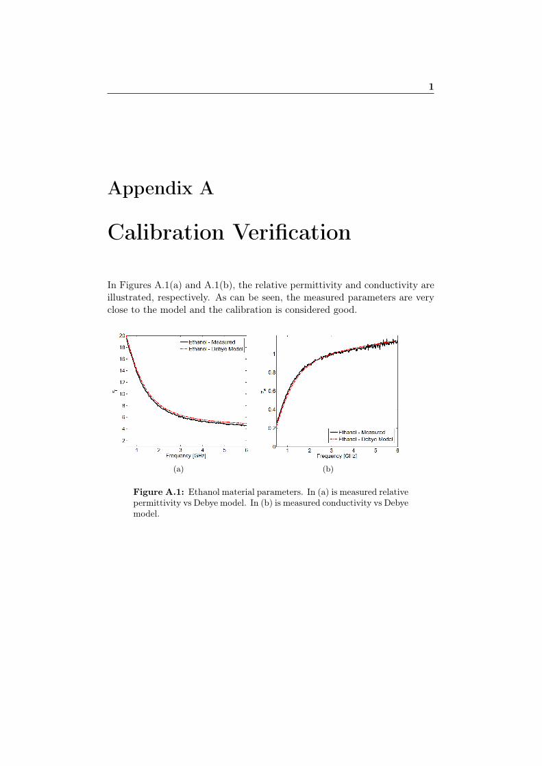
1
Appendix A
Calibration Verification
In Figures A.1(a) and A.1(b), the relative permittivity and conductivity areillustrated, respectively. As can be seen, the measured parameters are veryclose to the model and the calibration is considered good.
(a) (b)
Figure A.1: Ethanol material parameters. In (a) is measured relativepermittivity vs Debye model. In (b) is measured conductivity vs Debyemodel.
2
Appendix B
Fat Mimicking Media
In general for biological tissues, the conductivity of media follows the rel-ative permittivity, i.e. media with high permittivity tend to have higherconductivity. An example of this can be found in Table 3.1 where someaverage permittivity and conductivity values of some typical tissues at 2.45GHz were presented. Liquids that can emulate electromagnetic properties offat can be difficult to find due to fat’s combination of low conductivity andintermediate relative permittivity. For sanitary reasons, animal fat was notconsidered for the experimental setup.
Colza frying oil, that one could perhaps consider as a liquid fat, has e.g.ε′r = 3.2 and σ = 0.017 S/m at 2.45 GHz as can be seen in Figure C.1 inAppendix C. The conductivity of the oil is almost an order lower than thatof fat whereas water-based media typically have much higher ε′r and higherσ than fat.
For simplicity, 99.5% pure glycerin is utilized as a fat mimicking media.Glycerin is widely used as a coupling medium for microwave breast cancerimaging cameras and is therefore easily available for this project because sucha camera is in operation at the Department of Electrical Engineering, DTU.Glycerin is a thick liquid with vicosity that reminds of syrup. The dielectricproperties of glycerin are illustrated in Figure B.1. At around 2.45 GHz,ε′r = 5.8 and σ = 0.48 S/m. The relative permittivity of glycerin is slightlyhigher than that of fat and the conductivity is more than 4 times higher.This fat mimicking media can therefore, to some extent, be considered asthe effective fat, including both the skin layer as well as the fat layer. Therelatively high conductivity, however, causes much more attenuation in thephantom than would be expected in actual fat therefore, less power willpenetrate into the phantom. This must be considered when interpreting themeasurement results below.
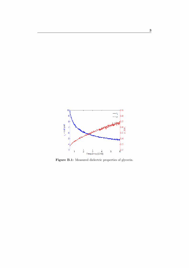
3
Figure B.1: Measured dielectric properties of glycerin.
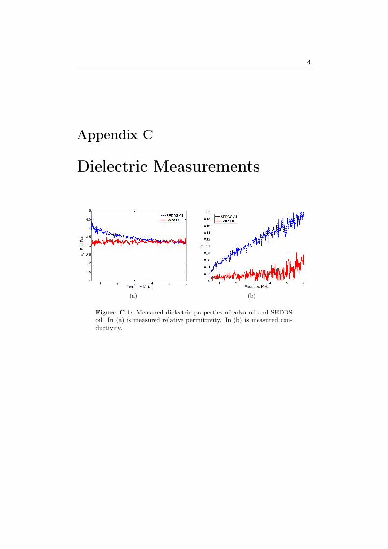
4
Appendix C
Dielectric Measurements
(a) (b)
Figure C.1: Measured dielectric properties of colza oil and SEDDSoil. In (a) is measured relative permittivity. In (b) is measured con-ductivity.

5
Appendix D
System Measurements
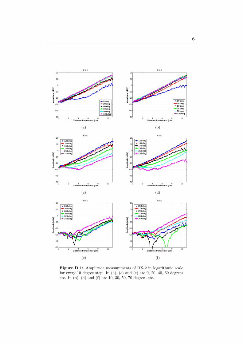
6
0 2 4 6 8 10−50
−40
−30
−20
−10
0
10
20RX−2
Distance from center [cm]
Am
plit
ud
e [d
BV
]
0 deg20 deg40 deg60 deg80 deg100 deg
(a)
0 2 4 6 8 10−50
−40
−30
−20
−10
0
10
20RX−2
Distance from center [cm]
Am
plit
ud
e [d
BV
]
10 deg30 deg50 deg70 deg90 deg110 deg
(b)
0 2 4 6 8 10−50
−40
−30
−20
−10
0
10
20RX−2
Distance from center [cm]
Am
plit
ud
e [d
BV
]
120 deg140 deg160 deg180 deg200 deg220 deg
(c)
0 2 4 6 8 10−50
−40
−30
−20
−10
0
10
20RX−2
Distance from center [cm]
Am
plit
ud
e [d
BV
]
130 deg150 deg170 deg190 deg210 deg230 deg
(d)
0 2 4 6 8 10−50
−40
−30
−20
−10
0
10
20RX−2
Distance from center [cm]
Am
plit
ud
e [d
BV
]
240 deg260 deg280 deg300 deg320 deg340 deg
(e)
0 2 4 6 8 10−50
−40
−30
−20
−10
0
10
20RX−2
Distance from center [cm]
Am
plit
ud
e [d
BV
]
250 deg270 deg290 deg310 deg330 deg350 deg
(f)
Figure D.1: Amplitude measurements of RX-2 in logarithmic scalefor every 10 degree step. In (a), (c) and (e) are 0, 20, 40, 60 degreesetc. In (b), (d) and (f) are 10, 30, 50, 70 degrees etc.
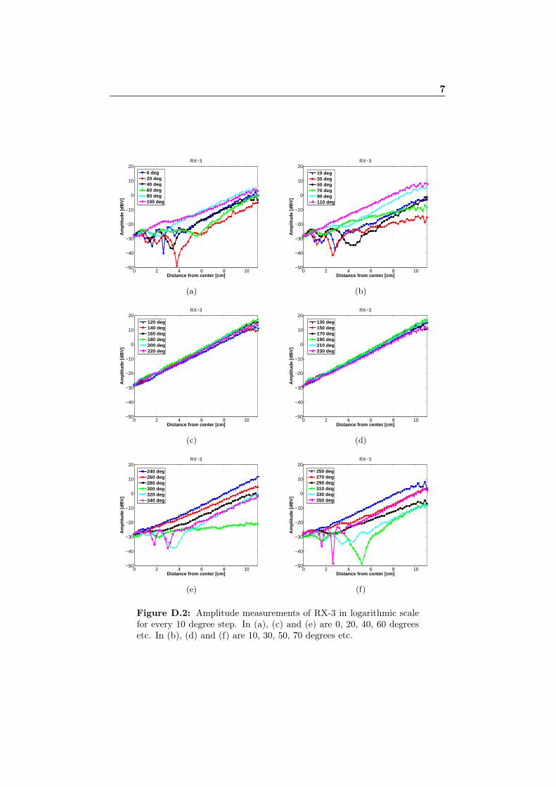
7
0 2 4 6 8 10−50
−40
−30
−20
−10
0
10
20RX−3
Distance from center [cm]
Am
plit
ud
e [d
BV
]
0 deg20 deg40 deg60 deg80 deg100 deg
(a)
0 2 4 6 8 10−50
−40
−30
−20
−10
0
10
20RX−3
Distance from center [cm]
Am
plit
ud
e [d
BV
]
10 deg30 deg50 deg70 deg90 deg110 deg
(b)
0 2 4 6 8 10−50
−40
−30
−20
−10
0
10
20RX−3
Distance from center [cm]
Am
plit
ud
e [d
BV
]
120 deg140 deg160 deg180 deg200 deg220 deg
(c)
0 2 4 6 8 10−50
−40
−30
−20
−10
0
10
20RX−3
Distance from center [cm]
Am
plit
ud
e [d
BV
]
130 deg150 deg170 deg190 deg210 deg230 deg
(d)
0 2 4 6 8 10−50
−40
−30
−20
−10
0
10
20RX−3
Distance from center [cm]
Am
plit
ud
e [d
BV
]
240 deg260 deg280 deg300 deg320 deg340 deg
(e)
0 2 4 6 8 10−50
−40
−30
−20
−10
0
10
20RX−3
Distance from center [cm]
Am
plit
ud
e [d
BV
]
250 deg270 deg290 deg310 deg330 deg350 deg
(f)
Figure D.2: Amplitude measurements of RX-3 in logarithmic scalefor every 10 degree step. In (a), (c) and (e) are 0, 20, 40, 60 degreesetc. In (b), (d) and (f) are 10, 30, 50, 70 degrees etc.
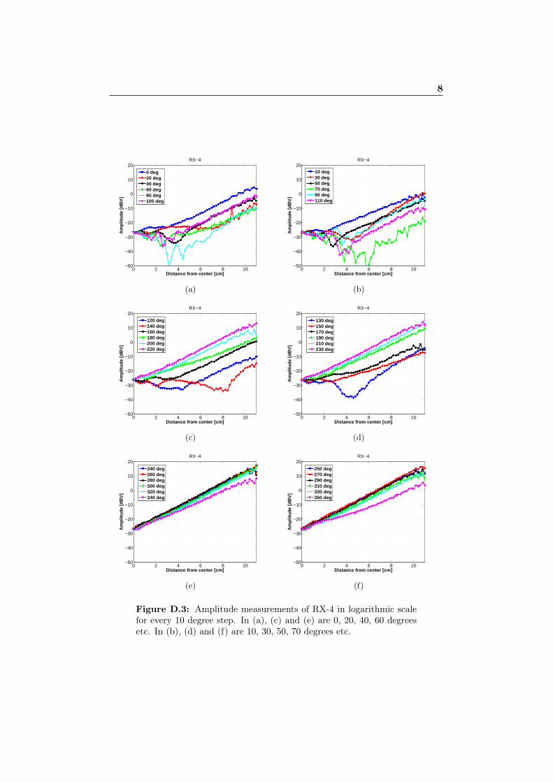
8
0 2 4 6 8 10−50
−40
−30
−20
−10
0
10
20RX−4
Distance from center [cm]
Am
plit
ud
e [d
BV
]
0 deg20 deg40 deg60 deg80 deg100 deg
(a)
0 2 4 6 8 10−50
−40
−30
−20
−10
0
10
20RX−4
Distance from center [cm]
Am
plit
ud
e [d
BV
]
10 deg30 deg50 deg70 deg90 deg110 deg
(b)
0 2 4 6 8 10−50
−40
−30
−20
−10
0
10
20RX−4
Distance from center [cm]
Am
plit
ud
e [d
BV
]
120 deg140 deg160 deg180 deg200 deg220 deg
(c)
0 2 4 6 8 10−50
−40
−30
−20
−10
0
10
20RX−4
Distance from center [cm]
Am
plit
ud
e [d
BV
]
130 deg150 deg170 deg190 deg210 deg230 deg
(d)
0 2 4 6 8 10−50
−40
−30
−20
−10
0
10
20RX−4
Distance from center [cm]
Am
plit
ud
e [d
BV
]
240 deg260 deg280 deg300 deg320 deg340 deg
(e)
0 2 4 6 8 10−50
−40
−30
−20
−10
0
10
20RX−4
Distance from center [cm]
Am
plit
ud
e [d
BV
]
250 deg270 deg290 deg310 deg330 deg350 deg
(f)
Figure D.3: Amplitude measurements of RX-4 in logarithmic scalefor every 10 degree step. In (a), (c) and (e) are 0, 20, 40, 60 degreesetc. In (b), (d) and (f) are 10, 30, 50, 70 degrees etc.
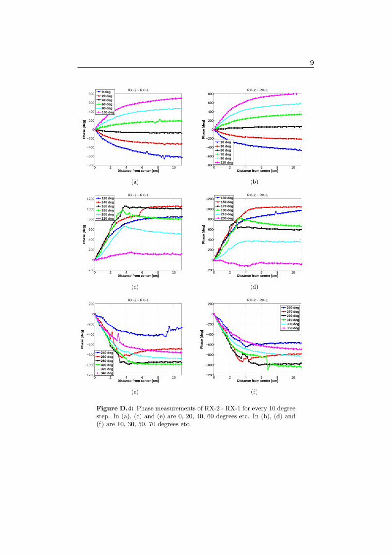
9
0 2 4 6 8 10−800
−600
−400
−200
0
200
400
600
800RX−2 − RX−1
Distance from center [cm]
Ph
ase
[deg
]
0 deg20 deg40 deg60 deg80 deg100 deg
(a)
0 2 4 6 8 10−800
−600
−400
−200
0
200
400
600
800RX−2 − RX−1
Distance from center [cm]
Ph
ase
[deg
]
10 deg30 deg50 deg70 deg90 deg110 deg
(b)
0 2 4 6 8 10−200
0
200
400
600
800
1000
1200RX−2 − RX−1
Distance from center [cm]
Ph
ase
[deg
]
120 deg140 deg160 deg180 deg200 deg220 deg
(c)
0 2 4 6 8 10−200
0
200
400
600
800
1000
1200RX−2 − RX−1
Distance from center [cm]
Ph
ase
[deg
]
130 deg150 deg170 deg190 deg210 deg230 deg
(d)
0 2 4 6 8 10−1200
−1000
−800
−600
−400
−200
0
200RX−2 − RX−1
Distance from center [cm]
Ph
ase
[deg
]
240 deg260 deg280 deg300 deg320 deg340 deg
(e)
0 2 4 6 8 10−1200
−1000
−800
−600
−400
−200
0
200RX−2 − RX−1
Distance from center [cm]
Ph
ase
[deg
]
250 deg270 deg290 deg310 deg330 deg350 deg
(f)
Figure D.4: Phase measurements of RX-2 - RX-1 for every 10 degreestep. In (a), (c) and (e) are 0, 20, 40, 60 degrees etc. In (b), (d) and(f) are 10, 30, 50, 70 degrees etc.
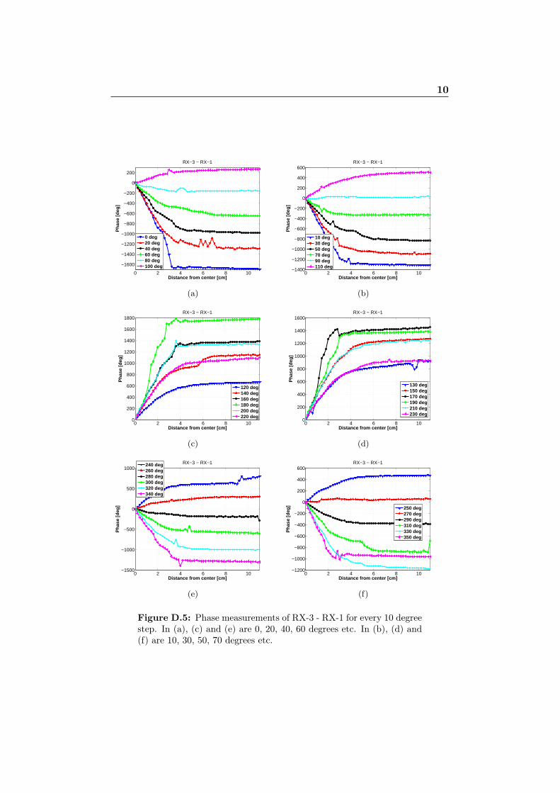
10
0 2 4 6 8 10
−1600
−1400
−1200
−1000
−800
−600
−400
−200
0
200
RX−3 − RX−1
Distance from center [cm]
Ph
ase
[deg
]
0 deg20 deg40 deg60 deg80 deg100 deg
(a)
0 2 4 6 8 10−1400
−1200
−1000
−800
−600
−400
−200
0
200
400
600RX−3 − RX−1
Distance from center [cm]
Ph
ase
[deg
]
10 deg30 deg50 deg70 deg90 deg110 deg
(b)
0 2 4 6 8 100
200
400
600
800
1000
1200
1400
1600
1800RX−3 − RX−1
Distance from center [cm]
Ph
ase
[deg
]
120 deg140 deg160 deg180 deg200 deg220 deg
(c)
0 2 4 6 8 100
200
400
600
800
1000
1200
1400
1600RX−3 − RX−1
Distance from center [cm]
Ph
ase
[deg
]
130 deg150 deg170 deg190 deg210 deg230 deg
(d)
0 2 4 6 8 10−1500
−1000
−500
0
500
1000RX−3 − RX−1
Distance from center [cm]
Ph
ase
[deg
]
240 deg260 deg280 deg300 deg320 deg340 deg
(e)
0 2 4 6 8 10−1200
−1000
−800
−600
−400
−200
0
200
400
600RX−3 − RX−1
Distance from center [cm]
Ph
ase
[deg
]
250 deg270 deg290 deg310 deg330 deg350 deg
(f)
Figure D.5: Phase measurements of RX-3 - RX-1 for every 10 degreestep. In (a), (c) and (e) are 0, 20, 40, 60 degrees etc. In (b), (d) and(f) are 10, 30, 50, 70 degrees etc.
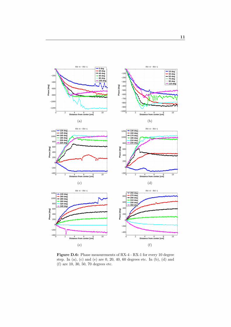
11
0 2 4 6 8 10
−1200
−1000
−800
−600
−400
−200
0RX−4 − RX−1
Distance from center [cm]
Ph
ase
[deg
]
0 deg20 deg40 deg60 deg80 deg100 deg
(a)
0 2 4 6 8 10−1000
−900
−800
−700
−600
−500
−400
−300
−200
−100
0RX−4 − RX−1
Distance from center [cm]
Ph
ase
[deg
]
10 deg30 deg50 deg70 deg90 deg110 deg
(b)
0 2 4 6 8 10−400
−200
0
200
400
600
800
1000
1200RX−4 − RX−1
Distance from center [cm]
Ph
ase
[deg
]
120 deg140 deg160 deg180 deg200 deg220 deg
(c)
0 2 4 6 8 10−200
0
200
400
600
800
1000
1200RX−4 − RX−1
Distance from center [cm]
Ph
ase
[deg
]
130 deg150 deg170 deg190 deg210 deg230 deg
(d)
0 2 4 6 8 10−400
−200
0
200
400
600
800
1000
1200RX−4 − RX−1
Distance from center [cm]
Ph
ase
[deg
]
240 deg260 deg280 deg300 deg320 deg340 deg
(e)
0 2 4 6 8 10
−400
−200
0
200
400
600
800
RX−4 − RX−1
Distance from center [cm]
Ph
ase
[deg
]
250 deg270 deg290 deg310 deg330 deg350 deg
(f)
Figure D.6: Phase measurements of RX-4 - RX-1 for every 10 degreestep. In (a), (c) and (e) are 0, 20, 40, 60 degrees etc. In (b), (d) and(f) are 10, 30, 50, 70 degrees etc.
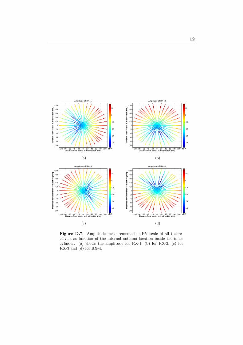
12
Distance from center in X−direction [mm]
Dis
tanc
e fr
om c
ente
r in
Y−d
irect
ion
[mm
]
Amplitude of RX−1
−100 −80 −60 −40 −20 0 20 40 60 80 100
−100
−80
−60
−40
−20
0
20
40
60
80
100
dBV
−40
−30
−20
−10
0
10
(a)
Distance from center in X−direction [mm]
Dis
tanc
e fr
om c
ente
r in
Y−d
irect
ion
[mm
]
Amplitude of RX−2
−100 −80 −60 −40 −20 0 20 40 60 80 100
−100
−80
−60
−40
−20
0
20
40
60
80
100
dBV
−40
−30
−20
−10
0
10
(b)
Distance from center in X−direction [mm]
Dis
tanc
e fr
om c
ente
r in
Y−d
irect
ion
[mm
]
Amplitude of RX−3
−100 −80 −60 −40 −20 0 20 40 60 80 100
−100
−80
−60
−40
−20
0
20
40
60
80
100
dBV
−40
−30
−20
−10
0
10
(c)
Distance from center in X−direction [mm]
Dis
tanc
e fr
om c
ente
r in
Y−d
irect
ion
[mm
]
Amplitude of RX−4
−100 −80 −60 −40 −20 0 20 40 60 80 100
−100
−80
−60
−40
−20
0
20
40
60
80
100
dBV
−40
−30
−20
−10
0
10
(d)
Figure D.7: Amplitude measurements in dBV scale of all the re-ceivers as function of the internal antenna location inside the innercylinder. (a) shows the amplitude for RX-1, (b) for RX-2, (c) forRX-3 and (d) for RX-4.
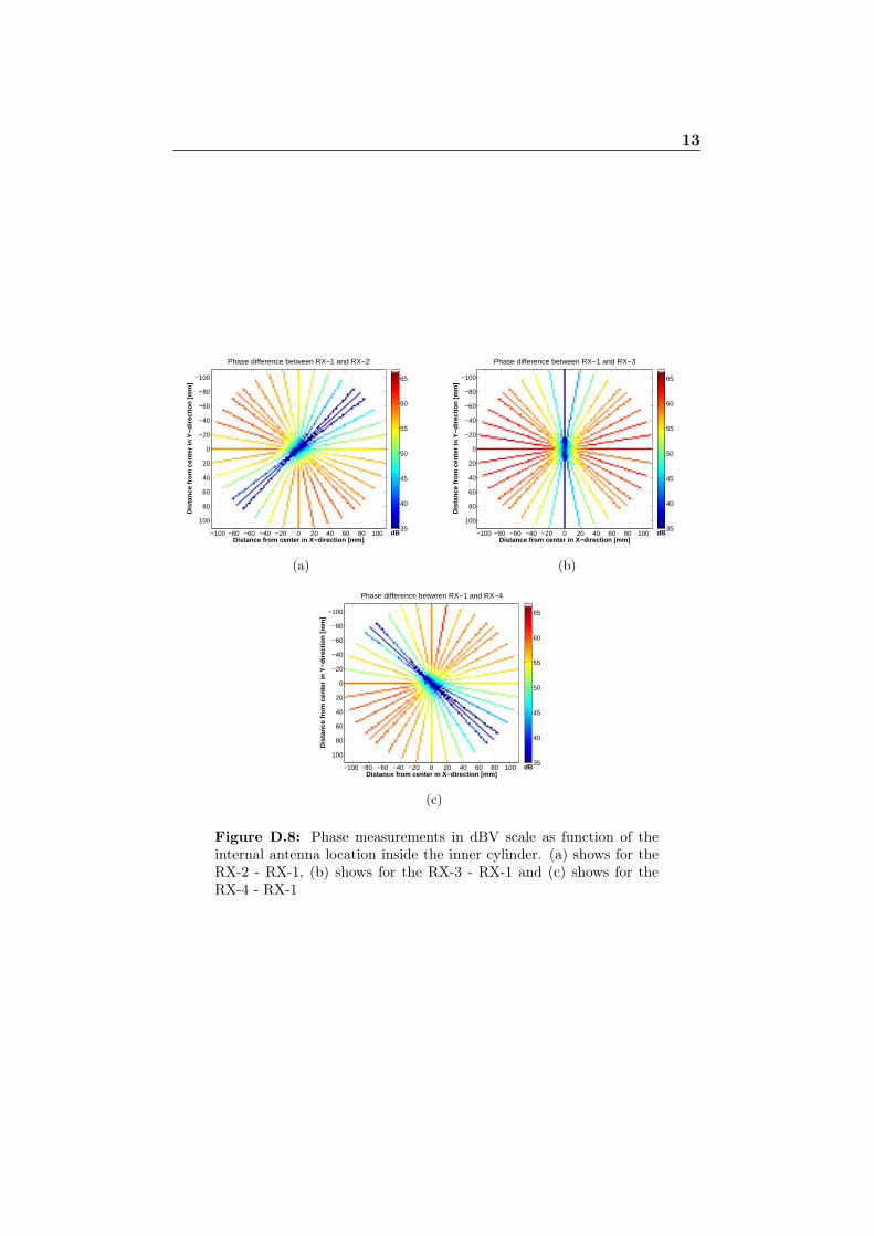
13
Distance from center in X−direction [mm]
Dis
tanc
e fr
om c
ente
r in
Y−d
irect
ion
[mm
]
Phase difference between RX−1 and RX−2
−100 −80 −60 −40 −20 0 20 40 60 80 100
−100
−80
−60
−40
−20
0
20
40
60
80
100
dB35
40
45
50
55
60
65
(a)
Distance from center in X−direction [mm]
Dis
tanc
e fr
om c
ente
r in
Y−d
irect
ion
[mm
]
Phase difference between RX−1 and RX−3
−100 −80 −60 −40 −20 0 20 40 60 80 100
−100
−80
−60
−40
−20
0
20
40
60
80
100
dB35
40
45
50
55
60
65
(b)
Distance from center in X−direction [mm]
Dis
tanc
e fr
om c
ente
r in
Y−d
irect
ion
[mm
]
Phase difference between RX−1 and RX−4
−100 −80 −60 −40 −20 0 20 40 60 80 100
−100
−80
−60
−40
−20
0
20
40
60
80
100
dB35
40
45
50
55
60
65
(c)
Figure D.8: Phase measurements in dBV scale as function of theinternal antenna location inside the inner cylinder. (a) shows for theRX-2 - RX-1, (b) shows for the RX-3 - RX-1 and (c) shows for theRX-4 - RX-1
14
Patent Application 1 [PA1]
Ingestible Capsule for Remote ControlledRelease of a Substance
Sævar Þór Jónasson
PatentOffice
: European Patent Office
PriorityDate
: 3. October 2012
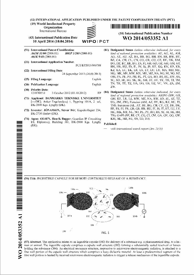


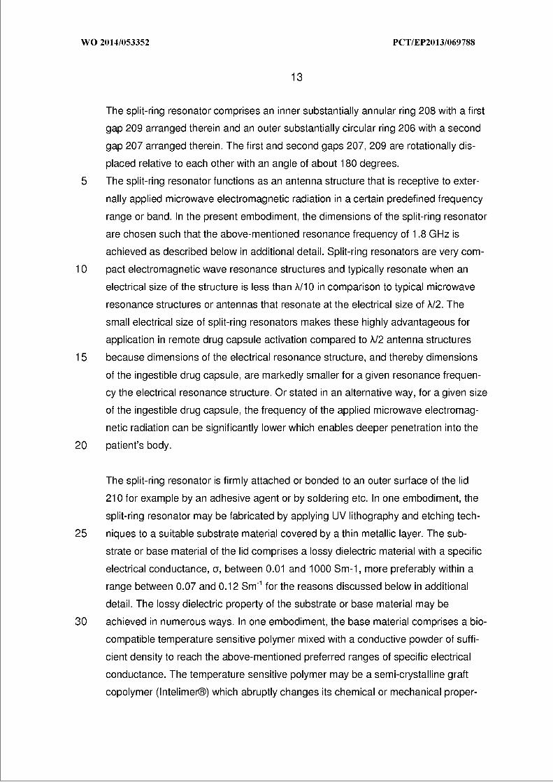
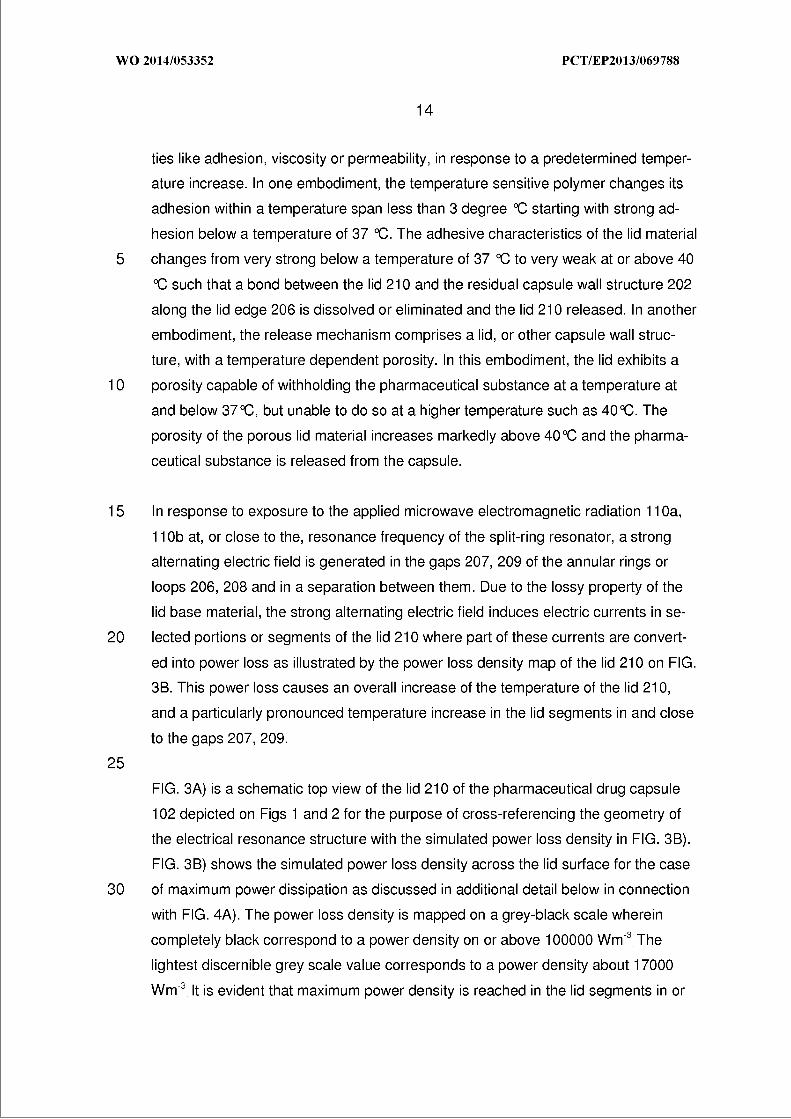
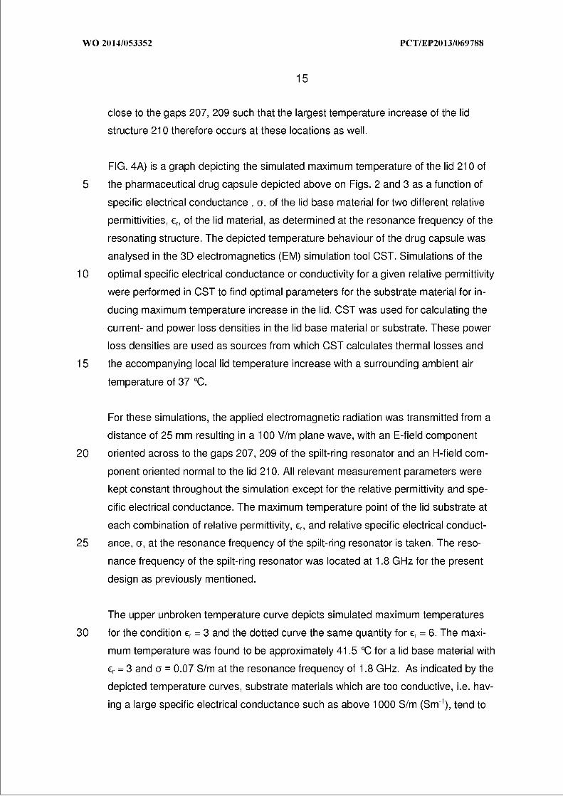
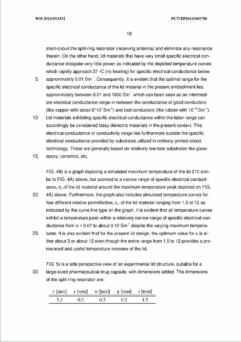
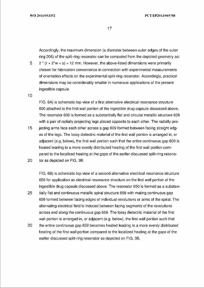


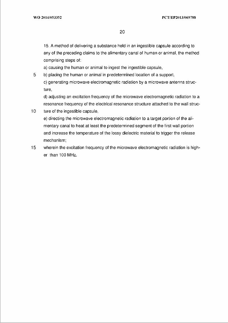
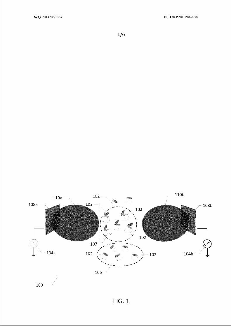
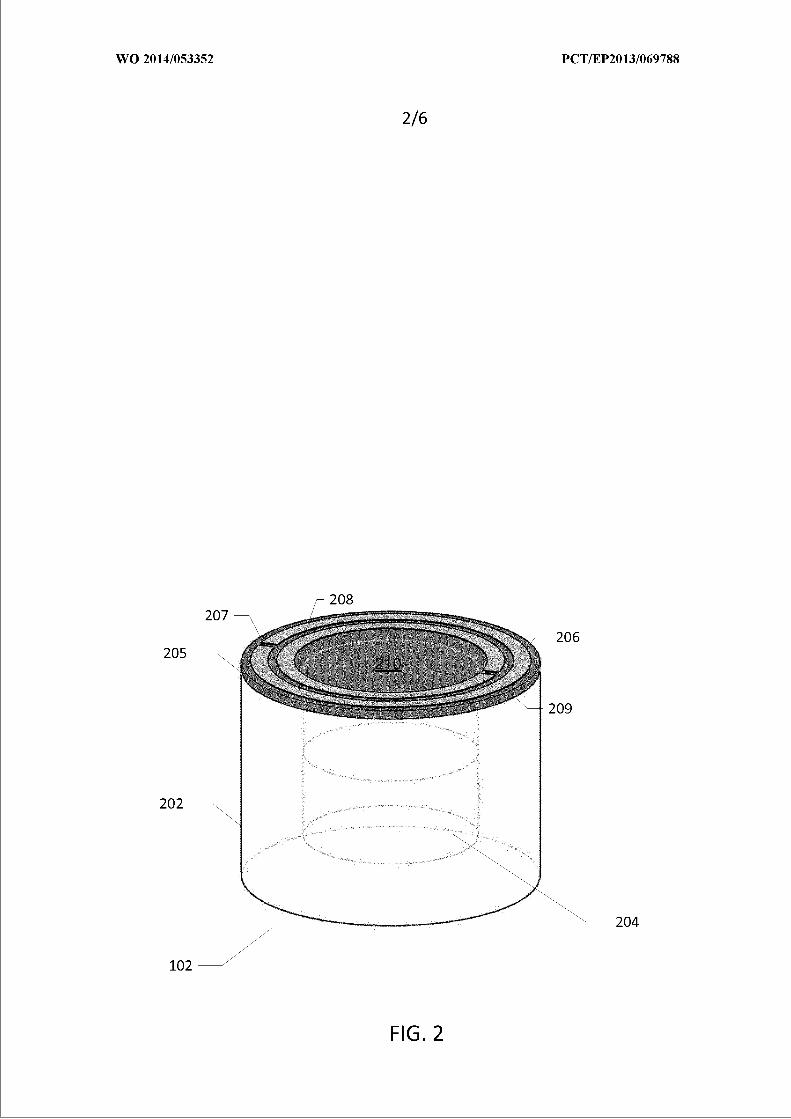
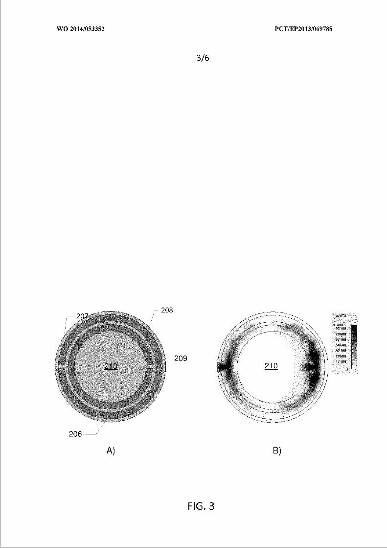
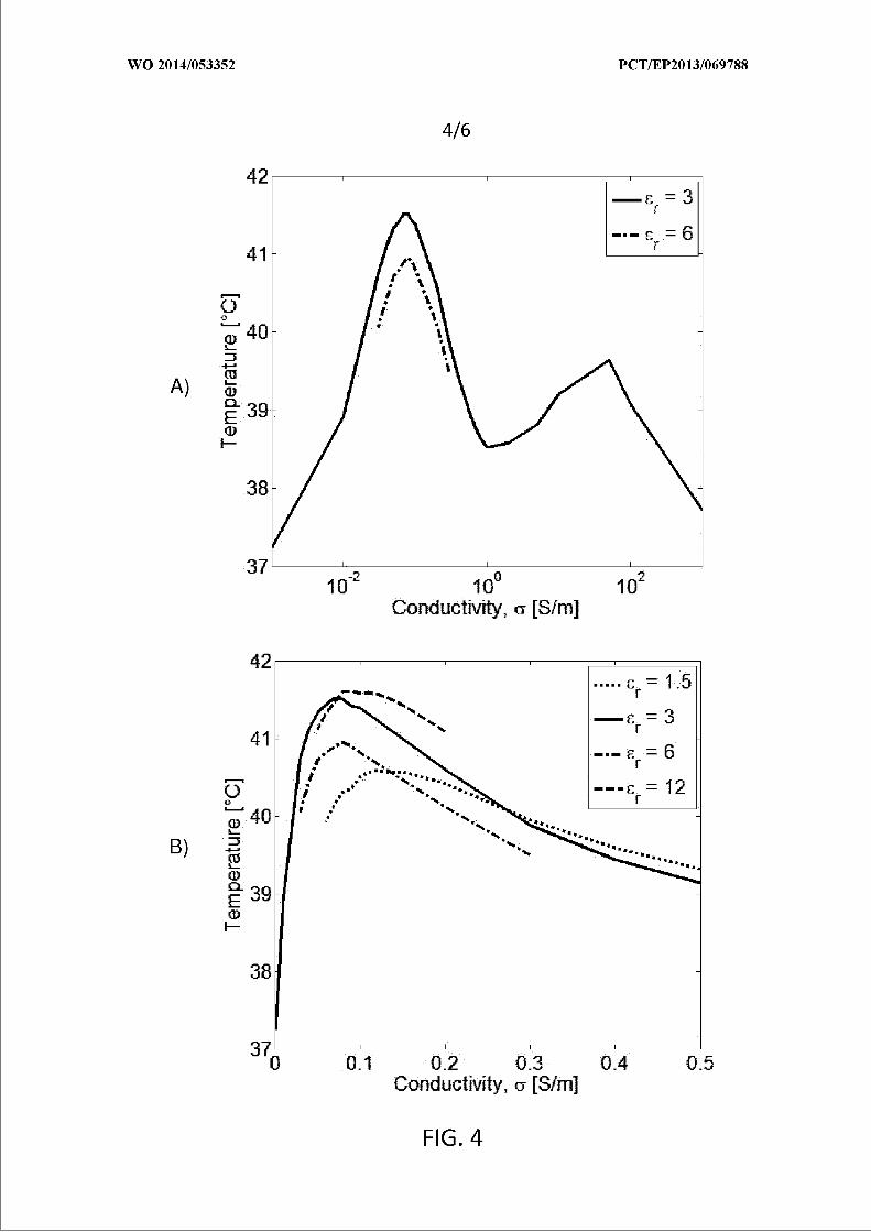
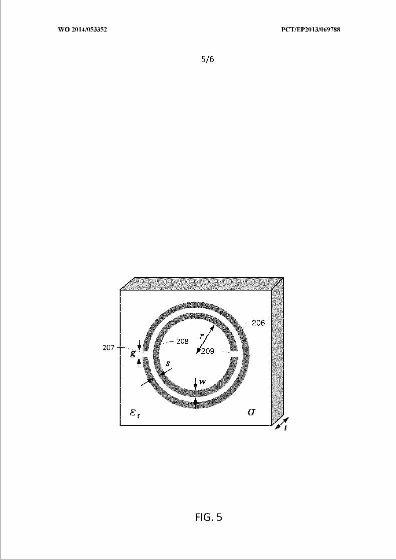
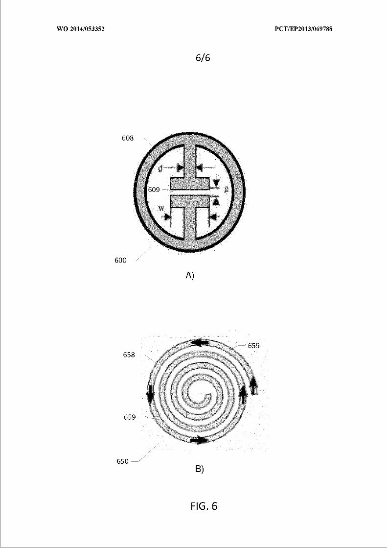

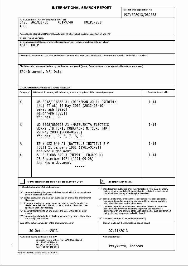
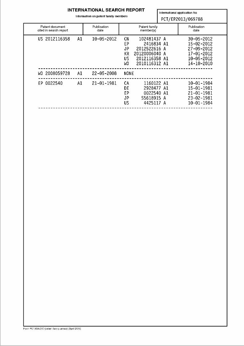
45
Conference Paper 1 [CP1]
Study of Split-Ring Resonators for use ona Pharmaceutical Drug Capsule forMicrowave Activated Drug Release
Sævar Þór Jónasson, Brian Sveistrup Jensenand Tom Keinicke Johansen
Conference:European Microwave Conference,Amsterdam RAI, The Netherlands,2012
Published : Oct. 2012
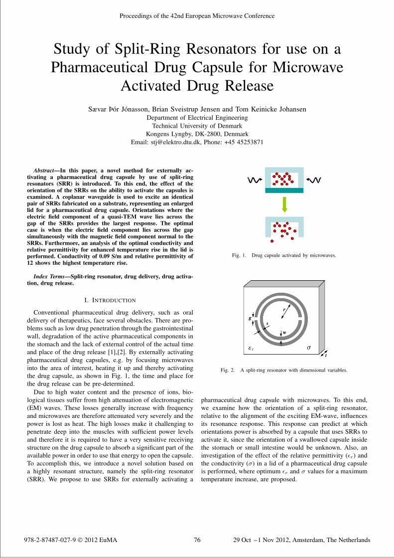
Study of Split-Ring Resonators for use on aPharmaceutical Drug Capsule for Microwave
Activated Drug ReleaseSævar Þór Jónasson, Brian Sveistrup Jensen and Tom Keinicke Johansen
Department of Electrical EngineeringTechnical University of Denmark
Kongens Lyngby, DK-2800, DenmarkEmail: [email protected], Phone: +45 45253871
Abstract—In this paper, a novel method for externally ac-tivating a pharmaceutical drug capsule by use of split-ringresonators (SRR) is introduced. To this end, the effect of theorientation of the SRRs on the ability to activate the capsules isexamined. A coplanar waveguide is used to excite an identicalpair of SRRs fabricated on a substrate, representing an enlargedlid for a pharmaceutical drug capsule. Orientations where theelectric field component of a quasi-TEM wave lies across thegap of the SRRs provides the largest response. The optimalcase is when the electric field component lies across the gapsimultaneously with the magnetic field component normal to theSRRs. Furthermore, an analysis of the optimal conductivity andrelative permittivity for enhanced temperature rise in the lid isperformed. Conductivity of 0.09 S/m and relative permittivity of12 shows the highest temperature rise.
Index Terms—Split-ring resonator, drug delivery, drug activa-tion, drug release.
I. INTRODUCTION
Conventional pharmaceutical drug delivery, such as oraldelivery of therapeutics, face several obstacles. There are pro-blems such as low drug penetration through the gastrointestinalwall, degradation of the active pharmaceutical components inthe stomach and the lack of external control of the actual timeand place of the drug release [1],[2]. By externally activatingpharmaceutical drug capsules, e.g. by focusing microwavesinto the area of interest, heating it up and thereby activatingthe drug capsule, as shown in Fig. 1, the time and place forthe drug release can be pre-determined.
Due to high water content and the presence of ions, bio-logical tissues suffer from high attenuation of electromagnetic(EM) waves. These losses generally increase with frequencyand microwaves are therefore attenuated very severely and thepower is lost as heat. The high losses make it challenging topenetrate deep into the muscles with sufficient power levelsand therefore it is required to have a very sensitive receivingstructure on the drug capsule to absorb a significant part of theavailable power in order to use that energy to open the capsule.To accomplish this, we introduce a novel solution based ona highly resonant structure, namely the split-ring resonator(SRR). We propose to use SRRs for externally activating a
Fig. 1. Drug capsule activated by microwaves.
Fig. 2. A split-ring resonator with dimensional variables.
pharmaceutical drug capsule with microwaves. To this end,we examine how the orientation of a split-ring resonator,relative to the alignment of the exciting EM-wave, influencesits resonance response. This response can predict at whichorientations power is absorbed by a capsule that uses SRRs toactivate it, since the orientation of a swallowed capsule insidethe stomach or small intestine would be unknown. Also, aninvestigation of the effect of the relative permittivity (εr) andthe conductivity (σ) in a lid of a pharmaceutical drug capsuleis performed, where optimum εr and σ values for a maximumtemperature increase, are proposed.
978-2-87487-027-9 © 2012 EuMA 29 Oct -1 Nov 2012, Amsterdam, The Netherlands
Proceedings of the 42nd European Microwave Conference
76
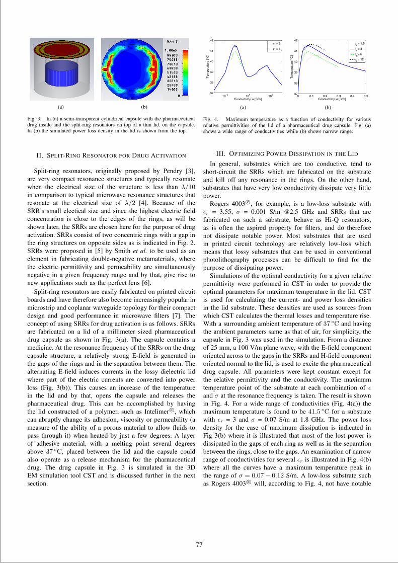
(a) (b)
Fig. 3. In (a) a semi-transparent cylindrical capsule with the pharmaceuticaldrug inside and the split-ring resonators on top of a thin lid, on the capsule.In (b) the simulated power loss density in the lid is shown from the top.
II. SPLIT-RING RESONATOR FOR DRUG ACTIVATION
Split-ring resonators, originally proposed by Pendry [3],are very compact resonance structures and typically resonatewhen the electrical size of the structure is less than λ/10in comparison to typical microwave resonance structures thatresonate at the electrical size of λ/2 [4]. Because of theSRR’s small electical size and since the highest electric fieldconcentration is close to the edges of the rings, as will beshown later, the SRRs are chosen here for the purpose of drugactivation. SRRs consist of two concentric rings with a gap inthe ring structures on opposite sides as is indicated in Fig. 2.SRRs were proposed in [5] by Smith et al. to be used as anelement in fabricating double-negative metamaterials, wherethe electric permittivity and permeability are simultaneouslynegative in a given frequency range and by that, give rise tonew applications such as the perfect lens [6].
Split-ring resonators are easily fabricated on printed circuitboards and have therefore also become increasingly popular inmicrostrip and coplanar waveguide topology for their compactdesign and good performance in microwave filters [7]. Theconcept of using SRRs for drug activation is as follows. SRRsare fabricated on a lid of a millimeter sized pharmaceuticaldrug capsule as shown in Fig. 3(a). The capsule contains amedicine. At the resonance frequency of the SRRs on the drugcapsule structure, a relatively strong E-field is generated inthe gaps of the rings and in the separation between them. Thealternating E-field induces currents in the lossy dielectric lidwhere part of the electric currents are converted into powerloss (Fig. 3(b)). This causes an increase of the temperaturein the lid and by that, opens the capsule and releases thepharmaceutical drug. This can be accomplished by havingthe lid constructed of a polymer, such as Intelimer R©, whichcan abruptly change its adhesion, viscosity or permeability (ameasure of the ability of a porous material to allow fluids topass through it) when heated by just a few degrees. A layerof adhesive material, with a melting point several degreesabove 37 C, placed between the lid and the capsule couldalso operate as a release mechanism for the pharmaceuticaldrug. The drug capsule in Fig. 3 is simulated in the 3DEM simulation tool CST and is discussed further in the nextsection.
10−2
100
102
37
38
39
40
41
42
Conductivity, σ [S/m]
Tem
pera
ture
[°C
]
εr = 3
εr = 6
(a)
0 0.1 0.2 0.3 0.4 0.537
38
39
40
41
42
Conductivity, σ [S/m]
Tem
pera
ture
[°C
]
εr = 1.5
εr = 3
εr = 6
εr = 12
(b)
Fig. 4. Maximum temperature as a function of conductivity for variousrelative permittivities of the lid of a pharmaceutical drug capsule. Fig. (a)shows a wide range of conductivities while (b) shows narrow range.
III. OPTIMIZING POWER DISSIPATION IN THE LID
In general, substrates which are too conductive, tend toshort-circuit the SRRs which are fabricated on the substrateand kill off any resonance in the rings. On the other hand,substrates that have very low conductivity dissipate very littlepower.
Rogers 4003 R©, for example, is a low-loss substrate withεr = 3.55, σ = 0.001 S/m @2.5 GHz and SRRs that arefabricated on such a substrate, behave as Hi-Q resonators,as is often the aspired property for filters, and do thereforenot dissipate notable power. Most substrates that are usedin printed circuit technology are relatively low-loss whichmeans that lossy substrates that can be used in conventionalphotolithography processes can be difficult to find for thepurpose of dissipating power.
Simulations of the optimal conductivity for a given relativepermittivity were performed in CST in order to provide theoptimal parameters for maximum temperature in the lid. CSTis used for calculating the current- and power loss densitiesin the lid substrate. These densities are used as sources fromwhich CST calculates the thermal losses and temperature rise.With a surrounding ambient temperature of 37 C and havingthe ambient parameters same as that of air, for simplicity, thecapsule in Fig. 3 was used in the simulation. From a distanceof 25 mm, a 100 V/m plane wave, with the E-field componentoriented across to the gaps in the SRRs and H-field componentoriented normal to the lid, is used to excite the pharmaceuticaldrug capsule. All parameters were kept constant except forthe relative permittivity and the conductivity. The maximumtemperature point of the substrate at each combination of εand σ at the resonance frequency is taken. The result is shownin Fig. 4. For a wide range of conductivities (Fig. 4(a)) themaximum temperature is found to be 41.5 C for a substratewith εr = 3 and σ = 0.07 S/m at 1.8 GHz. The power lossdensity for the case of maximum dissipation is indicated inFig 3(b) where it is illustrated that most of the lost power isdissipated in the gaps of each ring as well as in the separationbetween the rings, close to the gaps. An examination of narrowrange of conductivities for several εr is illustrated in Fig. 4(b)where all the curves have a maximum temperature peak inthe range of σ = 0.07− 0.12 S/m. A low-loss substrate suchas Rogers 4003 R© will, according to Fig. 4, not have notable
77
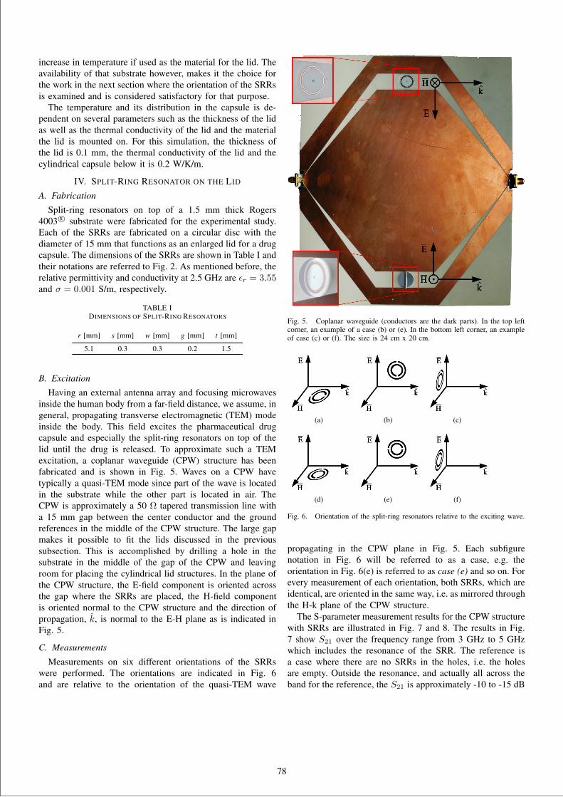
increase in temperature if used as the material for the lid. Theavailability of that substrate however, makes it the choice forthe work in the next section where the orientation of the SRRsis examined and is considered satisfactory for that purpose.
The temperature and its distribution in the capsule is de-pendent on several parameters such as the thickness of the lidas well as the thermal conductivity of the lid and the materialthe lid is mounted on. For this simulation, the thickness ofthe lid is 0.1 mm, the thermal conductivity of the lid and thecylindrical capsule below it is 0.2 W/K/m.
IV. SPLIT-RING RESONATOR ON THE LID
A. Fabrication
Split-ring resonators on top of a 1.5 mm thick Rogers4003 R© substrate were fabricated for the experimental study.Each of the SRRs are fabricated on a circular disc with thediameter of 15 mm that functions as an enlarged lid for a drugcapsule. The dimensions of the SRRs are shown in Table I andtheir notations are referred to Fig. 2. As mentioned before, therelative permittivity and conductivity at 2.5 GHz are εr = 3.55and σ = 0.001 S/m, respectively.
TABLE IDIMENSIONS OF SPLIT-RING RESONATORS
r [mm] s [mm] w [mm] g [mm] t [mm]
5.1 0.3 0.3 0.2 1.5
B. Excitation
Having an external antenna array and focusing microwavesinside the human body from a far-field distance, we assume, ingeneral, propagating transverse electromagnetic (TEM) modeinside the body. This field excites the pharmaceutical drugcapsule and especially the split-ring resonators on top of thelid until the drug is released. To approximate such a TEMexcitation, a coplanar waveguide (CPW) structure has beenfabricated and is shown in Fig. 5. Waves on a CPW havetypically a quasi-TEM mode since part of the wave is locatedin the substrate while the other part is located in air. TheCPW is approximately a 50 Ω tapered transmission line witha 15 mm gap between the center conductor and the groundreferences in the middle of the CPW structure. The large gapmakes it possible to fit the lids discussed in the previoussubsection. This is accomplished by drilling a hole in thesubstrate in the middle of the gap of the CPW and leavingroom for placing the cylindrical lid structures. In the plane ofthe CPW structure, the E-field component is oriented acrossthe gap where the SRRs are placed, the H-field componentis oriented normal to the CPW structure and the direction ofpropagation, k, is normal to the E-H plane as is indicated inFig. 5.
C. Measurements
Measurements on six different orientations of the SRRswere performed. The orientations are indicated in Fig. 6and are relative to the orientation of the quasi-TEM wave
Fig. 5. Coplanar waveguide (conductors are the dark parts). In the top leftcorner, an example of a case (b) or (e). In the bottom left corner, an exampleof case (c) or (f). The size is 24 cm x 20 cm.
(a) (b) (c)
(d) (e) (f)
Fig. 6. Orientation of the split-ring resonators relative to the exciting wave.
propagating in the CPW plane in Fig. 5. Each subfigurenotation in Fig. 6 will be referred to as a case, e.g. theorientation in Fig. 6(e) is referred to as case (e) and so on. Forevery measurement of each orientation, both SRRs, which areidentical, are oriented in the same way, i.e. as mirrored throughthe H-k plane of the CPW structure.
The S-parameter measurement results for the CPW structurewith SRRs are illustrated in Fig. 7 and 8. The results in Fig.7 show S21 over the frequency range from 3 GHz to 5 GHzwhich includes the resonance of the SRR. The reference isa case where there are no SRRs in the holes, i.e. the holesare empty. Outside the resonance, and actually all across theband for the reference, the S21 is approximately -10 to -15 dB
78
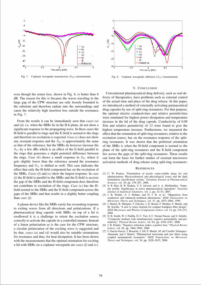
Fig. 7. Coplanar waveguide transmission (S21) measurement.
even though the return loss, shown in Fig. 8, is better than 6dB. The reason for this is because the waves traveling in thelarge gap of the CPW structure are only loosely bounded tothe substrate and therefore radiate into the surroundings andcause the relatively high insertion loss outside the resonancein Fig. 7.
From the results it can be immediately seen that cases (a)and (d), i.e. when the SRRs lie in the H-k plane, do not show asignificant response to the propagating wave. In these cases theH-field is parallel to rings and the E-field is normal to the ringsand therefore no excitation is expected. Case (c) does not showany resonant response and the S21 is approximately the sameas that of the reference, but the SRRs do however increase theS11 by a few dBs which is an effect of the E-field parallel tothe rings that generates a slight potential difference betweenthe rings. Case (b) shows a small response in S21 where itgets slightly lower than the reference around the resonancefrequency and S11 is shifted as well. This case indicates theeffect that only the H-field component has on the excitation ofthe SRRs. Cases (f) and (e) show the largest response. In case(f) the H-field is parallel to the SRRs and the E-field is accrossthe gap of the SRRs and the H-field component does thereforenot contribute to excitation of the rings. Case (e) has the H-field normal to the SRRs and the E-field component across thegaps of the SRRs and that results in a slightly better couplingthan case (f).
A planar device like the SRRs rarely has resonating responseto exiting waves from all directions and polarizations. If apharmaceutical drug capsule with SRRs on top of a lid isswallowed it is a challenge to orient the excitation sourcecorrectly to activate the capsule in a controlled manner. Insteadof a linear polarization as is the case for the CPW structure,a circular polarization of the exciting wave is suggested andby that, cases (a) and (d) would also be suitable orientationsfor resonance and thus, for heat dissipation. It has been shownwith the measurements that the optimal orientation for excitinga lid with SRRs on a coplanar waveguide are cases (f) and (e).
Fig. 8. Coplanar waveguide reflection (S11) measurement.
V. CONCLUSION
Conventional pharmaceutical drug delivery, such as oral de-livery of therapeutics, have problems such as external controlof the actual time and place of the drug release. In this paper,we introduced a method of externally activating parmaceuticaldrug capsules by use of split-ring resonators. For that purpose,the optimal electric conductivities and relative permittivitieswere simulated for highest power dissipation and temperatureincrease in the lid of the drug capsule. Conductivity of 0.09S/m and relative permittivity of 12 were found to give thehighest temperature increase. Furthermore, we measured theeffect that the orientation of split-ring resonators, relative to theexcitation source, has on the resonance response of the split-ring resonators. It was shown that the preferred orientationof the SRRs is when the H-field component is normal to theplane of the split-ring resonators and the E-field componentlies across the gaps of the split-ring resonators. These resultscan form the basis for further studies of external microwaveactivation methods of drug release using split-ring resonators.
REFERENCES
[1] C. W. Pouton, “Formulation of poorly water-soluble drugs for oraladministration: Physicochemical and physiological issues and the lipidformulation classification system,” European Journal of PharmaceuticalSciences, vol. 29, pp. 278–287, 2006.
[2] S. B. Bari, B. R. Kadam, Y. S. Jaiswal, and A. A. Shirkhedkar, “Impu-rity profile: Significance in active pharmaceutical ingredient,” EurasianJournal of Analytical Chemistry, vol. 2, pp. 32–53, 2007.
[3] J. B. Pendry, A. J. Holden, and D. J. R. et al., “Magnetism fromconductors and enhanced nonlinear phenomena,” IEEE Transactions onMicrowave Theory and Techniques, vol. 47, pp. 2075–2084, 1999.
[4] J. Martel, R. Marqués, F. Falcone, J. D. Baena, F. Medina, F. Martín, andM. Sorolla, “A new lc series element for compact bandpass filter design,”IEEE Microwave and Wireless Components Letters, vol. 14, pp. 210–212,2004.
[5] D. R. Smith, W. J. Padilla, D. C. Vier, S. C. Nemat-Nasser, and S. Schultz,“Composite medium with simultaneously negative permeability and per-mittivity,” Physical Review Letters, vol. 84, pp. 4184–4187, 2000.
[6] J. B. Pendry, “Negative refraction makes a perfect lens,” Physical ReviewLetters, vol. 85, pp. 3966–3969, 2000.
[7] J. García-García, J. Bonache, I. Gil, F. Martín, M. del Castillo Velázquez-Ahumada, and J. Martel, “Miniaturized microstrip and cpw filters usingcoupled metamaterial resonators,” IEEE Transactions on MicrowaveTheory and Techniques, vol. 54, pp. 2628–2635, 2006.
79
50
Conference Paper 2 [CP2]
Design and Characterization of aLow-Viscous Muscle Tissue Mimicking
Media at the ISM-band (2.4-2.48 GHz) forEasy Antenna Displacement in In Vitro
Measurements
Sævar Þór Jónasson, Tom Keinicke Johansenand Vitaliy Zhurbenko
Conference: Asia-Pacific Microwave Conference,Kaohsiung, Taiwan, 2012
Published : Dec. 2012.
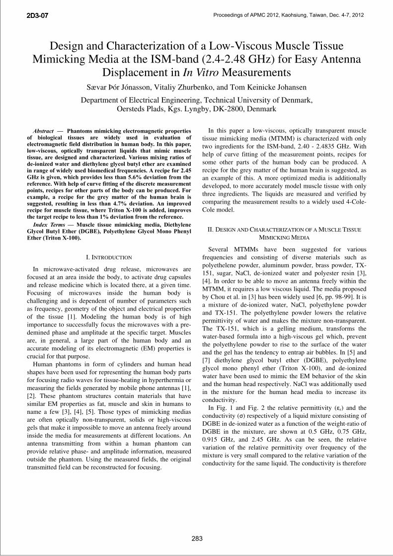
Design and Characterization of a Low-Viscous Muscle Tissue Mimicking Media at the ISM-band (2.4-2.48 GHz) for Easy Antenna
Displacement in In Vitro Measurements Sævar Þór Jónasson, Vitaliy Zhurbenko, and Tom Keinicke Johansen
Department of Electrical Engineering, Technical University of Denmark, Oersteds Plads, Kgs. Lyngby, DK-2800, Denmark
Abstract — Phantoms mimicking electromagnetic properties
of biological tissues are widely used in evaluation of electromagnetic field distribution in human body. In this paper, low-viscous, optically transparent liquids that mimic muscle tissue, are designed and characterized. Various mixing ratios of de-ionized water and diethylene glycol butyl ether are examined in range of widely used biomedical frequencies. A recipe for 2.45 GHz is given, which provides less than 5.6% deviation from the reference. With help of curve fitting of the discrete measurement points, recipes for other parts of the body can be produced. For example, a recipe for the grey matter of the human brain is suggested, resulting in less than 4.7% deviation. An improved recipe for muscle tissue, where Triton X-100 is added, improves the target recipe to less than 1% deviation from the reference.
Index Terms — Muscle tissue mimicking media, Diethylene Glycol Butyl Ether (DGBE), Polyethylene Glycol Mono Phenyl Ether (Triton X-100).
I. INTRODUCTION
In microwave-activated drug release, microwaves are focused at an area inside the body, to activate drug capsules and release medicine which is located there, at a given time. Focusing of microwaves inside the human body is challenging and is dependent of number of parameters such as frequency, geometry of the object and electrical properties of the tissue [1]. Modeling the human body is of high importance to successfully focus the microwaves with a pre-demined phase and amplitude at the specific target. Muscles are, in general, a large part of the human body and an accurate modeling of its electromagnetic (EM) properties is crucial for that purpose.
Human phantoms in form of cylinders and human head shapes have been used for representing the human body parts for focusing radio waves for tissue-heating in hyperthermia or measuring the fields generated by mobile phone antennas [1], [2]. These phantom structures contain materials that have similar EM properties as fat, muscle and skin in humans to name a few [3], [4], [5]. Those types of mimicking medias are often optically non-transparent, solids or high-viscous gels that make it impossible to move an antenna freely around inside the media for measurements at different locations. An antenna transmitting from within a human phantom can provide relative phase- and amplitude information, measured outside the phantom. Using the measured fields, the original transmitted field can be reconstructed for focusing.
In this paper a low-viscous, optically transparent muscle tissue mimicking media (MTMM) is characterized with only two ingredients for the ISM-band, 2.40 - 2.4835 GHz. With help of curve fitting of the measurement points, recipes for some other parts of the human body can be produced. A recipe for the grey matter of the human brain is suggested, as an example of this. A more optimized media is additionally developed, to more accurately model muscle tissue with only three ingredients. The liquids are measured and verified by comparing the measurement results to a widely used 4-Cole-Cole model.
II. DESIGN AND CHARACTERIZATION OF A MUSCLE TISSUE
MIMICKING MEDIA
Several MTMMs have been suggested for various frequencies and consisting of diverse materials such as polyethelene powder, aluminum powder, brass powder, TX-151, sugar, NaCl, de-ionized water and polyester resin [3], [4]. In order to be able to move an antenna freely within the MTMM, it requires a low viscous liquid. The media proposed by Chou et al. in [3] has been widely used [6, pp. 98-99]. It is a mixture of de-ionized water, NaCl, polyethylene powder and TX-151. The polyethylene powder lowers the relative permittivity of water and makes the mixture non-transparent. The TX-151, which is a gelling medium, transforms the water-based formula into a high-viscous gel which, prevent the polyethylene powder to rise to the surface of the water and the gel has the tendency to entrap air bubbles. In [5] and [7] diethylene glycol butyl ether (DGBE), polyethylene glycol mono phenyl ether (Triton X-100), and de-ionized water have been used to mimic the EM behavior of the skin and the human head respectively. NaCl was additionally used in the mixture for the human head media to increase its conductivity.
In Fig. 1 and Fig. 2 the relative permittivity ( r) and the conductivity ( ) respectively of a liquid mixture consisting of DGBE in de-ionized water as a function of the weight-ratio of DGBE in the mixture, are shown at 0.5 GHz, 0.75 GHz, 0.915 GHz, and 2.45 GHz. As can be seen, the relative variation of the relative permittivity over frequency of the mixture is very small compared to the relative variation of the conductivity for the same liquid. The conductivity is therefore
283
2D3-072D3-072D3-072D3-07 Proceedings of APMC 2012, Kaohsiung, Taiwan, Dec. 4-7, 2012
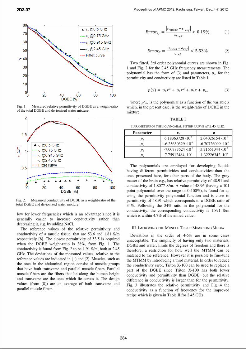
low for lower frequencies which is an advantage since it is generally easier to increase conductivity rather than decreasing it, e.g. by adding NaCl.
The reference values of the relative permittivity and conductivity of a muscle tissue, that are 53.6 and 1.81 S/m respectively [8]. The closest permittivity of 53.5 is acquired when the DGBE weight-ratio is 28%, from Fig. 1. The conductivity is found from Fig. 2 to be 1.91 S/m, both at 2.45 GHz. The deviations of the measured values, relative to the reference values are indicated in (1) and (2). Muscles, such as the ones in the abdominal region consist of muscle groups that have both transverse and parallel muscle fibers. Parallel muscle fibers are the fibers that lie along the human height and transverse are the ones which lie across it. The design values (from [8]) are an average of both transverse and parallel muscle fibers.
, (1)
. (2)
Two fitted, 3rd order polynomial curves are shown in Fig. 1 and Fig. 2 for the 2.45 GHz frequency measurements. The polynomial has the form of (3) and parameters, pn, for the permittivity and conductivity are listed in Table I.
, (3)
where p(x) is the polynomial as a function of the variable x which, in the present case, is the weight-ratio of DGBE in the mixture.
TABLE I
PARAMETERS OF THE POLYNOMIAL FITTED CURVE AT 2.45 GHZ.
Parameter r p1 6.18363728 ·10-5 2.04026154 ·10-6 p2 -6.25630329 ·10-3 -6.70726099 ·10-4 p3 -7.00787624 ·10-1 3.71651344 ·10-2 p4 7.75912484 ·101 1.32226342 ·100
The polynomials are employed for developing liquids
having different permittivities and conductivities than the ones presented here, for other parts of the body. The grey matter of the brain e.g., has relative permittivity of 48.91 and conductivity of 1.8077 S/m. A value of 48.96 (having a 101 point polynomial over the range of 0-100%), is found for r, using the permittivity polynomial function and is close to permittivity of 48.91 which corresponds to a DGBE ratio of 34%. Following the 34% ratio in the polynomial for the conductivity, the corresponding conductivity is 1.891 S/m which is within 4.7% of the aimed value.
III. IMPROVING THE MUSCLE TISSUE MIMICKING MEDIA
Deviations in the order of 4-6% are in some cases unacceptable. The simplicity of having only two materials, DGBE and water, limits the degrees of freedom and there is therefore, a restriction for how well the MTMM can be matched to the reference. However it is possible to fine-tune the MTMM by introducing a third material. In order to reduce the conductivity error, Triton X-100 can be used to replace a part of the DGBE since Triton X-100 has both lower conductivity and permittivity than DGBE, but the relative difference in conductivity is larger than for the permittivity. Fig. 3 illustrates the relative permittivity and Fig. 4 the conductivity as a function of frequency for the improved recipe which is given in Table II for 2.45 GHz.
Fig. 2. Measured conductivity of DGBE as a weight-ratio of the total DGBE and de-ionized water mixture.
Fig. 1. Measured relative permittivity of DGBE as a weight-ratio of the total DGBE and de-ionized water mixture.
284
2D3-072D3-072D3-072D3-07 Proceedings of APMC 2012, Kaohsiung, Taiwan, Dec. 4-7, 2012
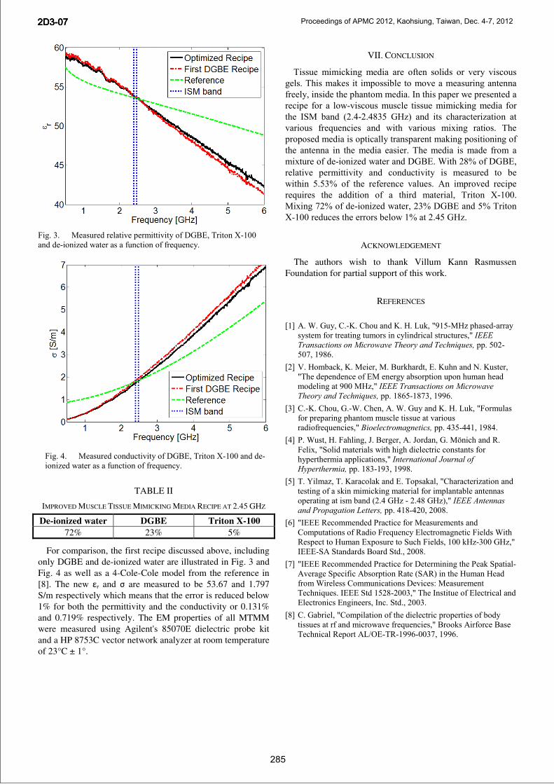
TABLE II
IMPROVED MUSCLE TISSUE MIMICKING MEDIA RECIPE AT 2.45 GHZ
De-ionized water DGBE Triton X-100 72% 23% 5%
For comparison, the first recipe discussed above, including only DGBE and de-ionized water are illustrated in Fig. 3 and Fig. 4 as well as a 4-Cole-Cole model from the reference in [8]. The new r and are measured to be 53.67 and 1.797 S/m respectively which means that the error is reduced below 1% for both the permittivity and the conductivity or 0.131% and 0.719% respectively. The EM properties of all MTMM were measured using Agilent's 85070E dielectric probe kit and a HP 8753C vector network analyzer at room temperature of 23°C ± 1°.
VII. CONCLUSION
Tissue mimicking media are often solids or very viscous gels. This makes it impossible to move a measuring antenna freely, inside the phantom media. In this paper we presented a recipe for a low-viscous muscle tissue mimicking media for the ISM band (2.4-2.4835 GHz) and its characterization at various frequencies and with various mixing ratios. The proposed media is optically transparent making positioning of the antenna in the media easier. The media is made from a mixture of de-ionized water and DGBE. With 28% of DGBE, relative permittivity and conductivity is measured to be within 5.53% of the reference values. An improved recipe requires the addition of a third material, Triton X-100. Mixing 72% of de-ionized water, 23% DGBE and 5% Triton X-100 reduces the errors below 1% at 2.45 GHz.
ACKNOWLEDGEMENT
The authors wish to thank Villum Kann Rasmussen Foundation for partial support of this work.
REFERENCES
[1] A. W. Guy, C.-K. Chou and K. H. Luk, "915-MHz phased-array system for treating tumors in cylindrical structures," IEEE Transactions on Microwave Theory and Techniques, pp. 502-507, 1986.
[2] V. Homback, K. Meier, M. Burkhardt, E. Kuhn and N. Kuster, "The dependence of EM energy absorption upon human head modeling at 900 MHz," IEEE Transactions on Microwave Theory and Techniques, pp. 1865-1873, 1996.
[3] C.-K. Chou, G.-W. Chen, A. W. Guy and K. H. Luk, "Formulas for preparing phantom muscle tissue at various radiofrequencies," Bioelectromagnetics, pp. 435-441, 1984.
[4] P. Wust, H. Fahling, J. Berger, A. Jordan, G. Mönich and R. Felix, "Solid materials with high dielectric constants for hyperthermia applications," International Journal of Hyperthermia, pp. 183-193, 1998.
[5] T. Yilmaz, T. Karacolak and E. Topsakal, "Characterization and testing of a skin mimicking material for implantable antennas operating at ism band (2.4 GHz - 2.48 GHz)," IEEE Antennas and Propagation Letters, pp. 418-420, 2008.
[6] "IEEE Recommended Practice for Measurements and Computations of Radio Frequency Electromagnetic Fields With Respect to Human Exposure to Such Fields, 100 kHz-300 GHz," IEEE-SA Standards Board Std., 2008.
[7] "IEEE Recommended Practice for Determining the Peak Spatial-Average Specific Absorption Rate (SAR) in the Human Head from Wireless Communications Devices: Measurement Techniques. IEEE Std 1528-2003," The Institue of Electrical and Electronics Engineers, Inc. Std., 2003.
[8] C. Gabriel, "Compilation of the dielectric properties of body tissues at rf and microwave frequencies," Brooks Airforce Base Technical Report AL/OE-TR-1996-0037, 1996.
Fig. 3. Measured relative permittivity of DGBE, Triton X-100 and de-ionized water as a function of frequency.
Fig. 4. Measured conductivity of DGBE, Triton X-100 and de-ionized water as a function of frequency.
285
2D3-072D3-072D3-072D3-07 Proceedings of APMC 2012, Kaohsiung, Taiwan, Dec. 4-7, 2012
54
Conference Paper 3 [CP3]
Microwave Assisted Drug Delivery
Sævar Þór Jónasson, Vitaliy Zhurbenkoand Tom Keinicke Johansen
Conference: URSI General Assembly and ScientificSymposium
Accepted : Aug. 2014
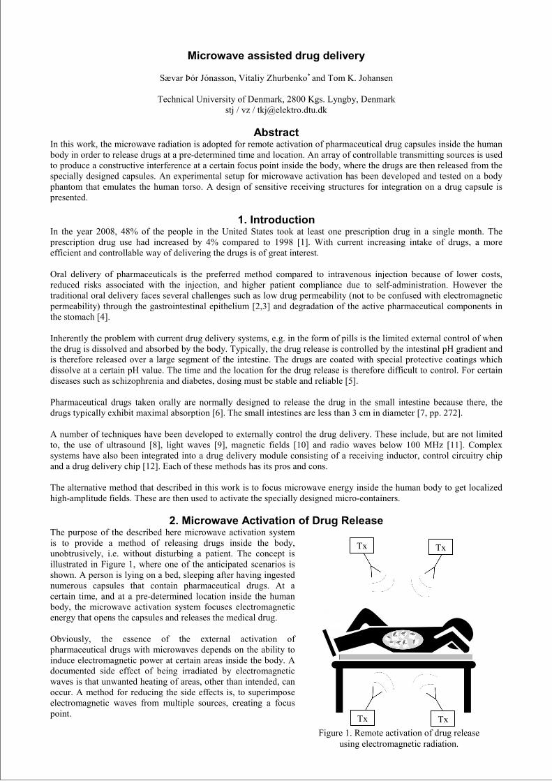
Microwave assisted drug delivery
Sævar Þór Jónasson, Vitaliy Zhurbenko* and Tom K. Johansen
Technical University of Denmark, 2800 Kgs. Lyngby, Denmark stj / vz / [email protected]
Abstract
In this work, the microwave radiation is adopted for remote activation of pharmaceutical drug capsules inside the human body in order to release drugs at a pre-determined time and location. An array of controllable transmitting sources is used to produce a constructive interference at a certain focus point inside the body, where the drugs are then released from the specially designed capsules. An experimental setup for microwave activation has been developed and tested on a body phantom that emulates the human torso. A design of sensitive receiving structures for integration on a drug capsule is presented.
1. Introduction In the year 2008, 48% of the people in the United States took at least one prescription drug in a single month. The prescription drug use had increased by 4% compared to 1998 [1]. With current increasing intake of drugs, a more efficient and controllable way of delivering the drugs is of great interest. Oral delivery of pharmaceuticals is the preferred method compared to intravenous injection because of lower costs, reduced risks associated with the injection, and higher patient compliance due to self-administration. However the traditional oral delivery faces several challenges such as low drug permeability (not to be confused with electromagnetic permeability) through the gastrointestinal epithelium [2,3] and degradation of the active pharmaceutical components in the stomach [4]. Inherently the problem with current drug delivery systems, e.g. in the form of pills is the limited external control of when the drug is dissolved and absorbed by the body. Typically, the drug release is controlled by the intestinal pH gradient and is therefore released over a large segment of the intestine. The drugs are coated with special protective coatings which dissolve at a certain pH value. The time and the location for the drug release is therefore difficult to control. For certain diseases such as schizophrenia and diabetes, dosing must be stable and reliable [5]. Pharmaceutical drugs taken orally are normally designed to release the drug in the small intestine because there, the drugs typically exhibit maximal absorption [6]. The small intestines are less than 3 cm in diameter [7, pp. 272]. A number of techniques have been developed to externally control the drug delivery. These include, but are not limited to, the use of ultrasound [8], light waves [9], magnetic fields [10] and radio waves below 100 MHz [11]. Complex systems have also been integrated into a drug delivery module consisting of a receiving inductor, control circuitry chip and a drug delivery chip [12]. Each of these methods has its pros and cons. The alternative method that described in this work is to focus microwave energy inside the human body to get localized high-amplitude fields. These are then used to activate the specially designed micro-containers.
2. Microwave Activation of Drug Release The purpose of the described here microwave activation system is to provide a method of releasing drugs inside the body, unobtrusively, i.e. without disturbing a patient. The concept is illustrated in Figure 1, where one of the anticipated scenarios is shown. A person is lying on a bed, sleeping after having ingested numerous capsules that contain pharmaceutical drugs. At a certain time, and at a pre-determined location inside the human body, the microwave activation system focuses electromagnetic energy that opens the capsules and releases the medical drug. Obviously, the essence of the external activation of pharmaceutical drugs with microwaves depends on the ability to induce electromagnetic power at certain areas inside the body. A documented side effect of being irradiated by electromagnetic waves is that unwanted heating of areas, other than intended, can occur. A method for reducing the side effects is, to superimpose electromagnetic waves from multiple sources, creating a focus point.
Figure 1. Remote activation of drug release using electromagnetic radiation.
Tx Tx
Tx Tx
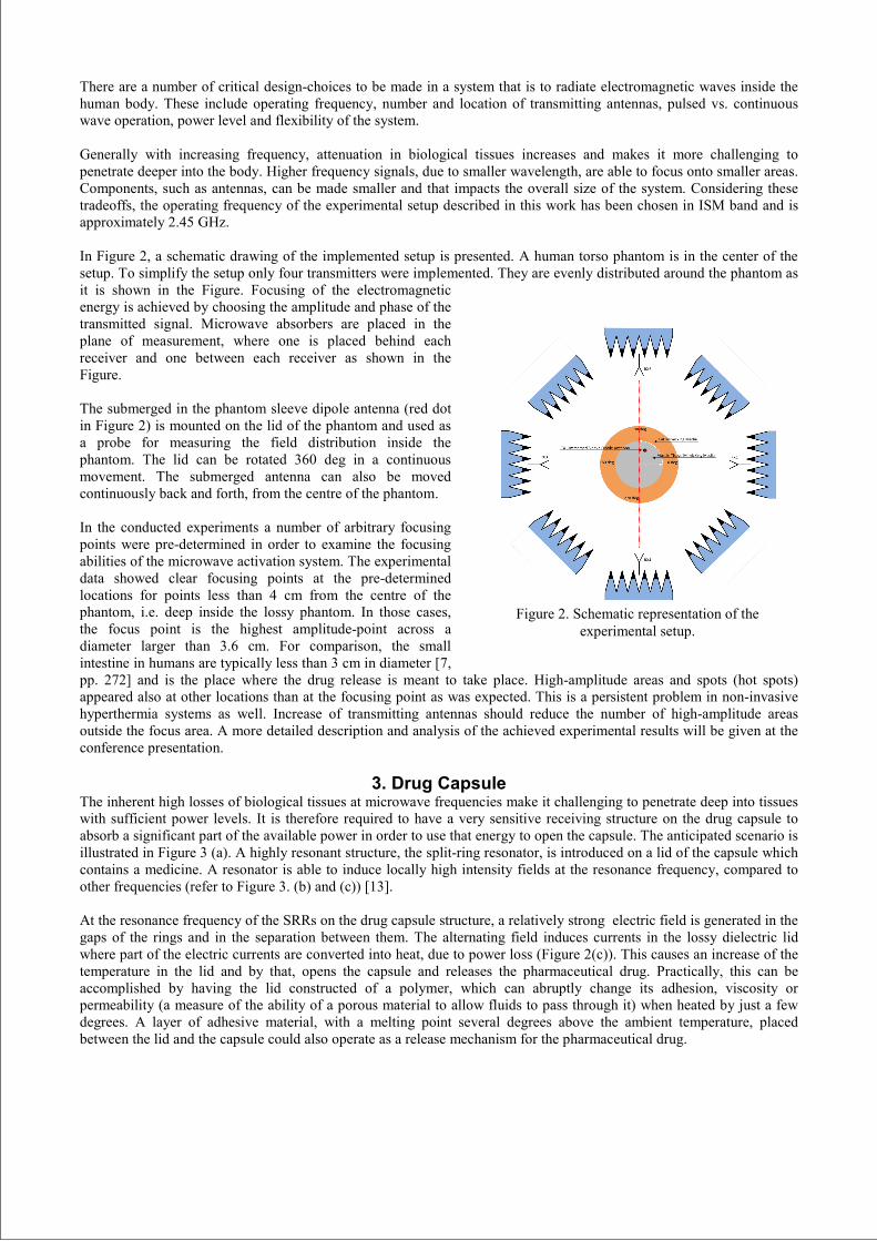
There are a number of critical design-choices to be made in a system that is to radiate electromagnetic waves inside the human body. These include operating frequency, number and location of transmitting antennas, pulsed vs. continuous wave operation, power level and flexibility of the system. Generally with increasing frequency, attenuation in biological tissues increases and makes it more challenging to penetrate deeper into the body. Higher frequency signals, due to smaller wavelength, are able to focus onto smaller areas. Components, such as antennas, can be made smaller and that impacts the overall size of the system. Considering these tradeoffs, the operating frequency of the experimental setup described in this work has been chosen in ISM band and is approximately 2.45 GHz. In Figure 2, a schematic drawing of the implemented setup is presented. A human torso phantom is in the center of the setup. To simplify the setup only four transmitters were implemented. They are evenly distributed around the phantom as it is shown in the Figure. Focusing of the electromagnetic energy is achieved by choosing the amplitude and phase of the transmitted signal. Microwave absorbers are placed in the plane of measurement, where one is placed behind each receiver and one between each receiver as shown in the Figure. The submerged in the phantom sleeve dipole antenna (red dot in Figure 2) is mounted on the lid of the phantom and used as a probe for measuring the field distribution inside the phantom. The lid can be rotated 360 deg in a continuous movement. The submerged antenna can also be moved continuously back and forth, from the centre of the phantom. In the conducted experiments a number of arbitrary focusing points were pre-determined in order to examine the focusing abilities of the microwave activation system. The experimental data showed clear focusing points at the pre-determined locations for points less than 4 cm from the centre of the phantom, i.e. deep inside the lossy phantom. In those cases, the focus point is the highest amplitude-point across a diameter larger than 3.6 cm. For comparison, the small intestine in humans are typically less than 3 cm in diameter [7, pp. 272] and is the place where the drug release is meant to take place. High-amplitude areas and spots (hot spots) appeared also at other locations than at the focusing point as was expected. This is a persistent problem in non-invasive hyperthermia systems as well. Increase of transmitting antennas should reduce the number of high-amplitude areas outside the focus area. A more detailed description and analysis of the achieved experimental results will be given at the conference presentation.
3. Drug Capsule The inherent high losses of biological tissues at microwave frequencies make it challenging to penetrate deep into tissues with sufficient power levels. It is therefore required to have a very sensitive receiving structure on the drug capsule to absorb a significant part of the available power in order to use that energy to open the capsule. The anticipated scenario is illustrated in Figure 3 (a). A highly resonant structure, the split-ring resonator, is introduced on a lid of the capsule which contains a medicine. A resonator is able to induce locally high intensity fields at the resonance frequency, compared to other frequencies (refer to Figure 3. (b) and (c)) [13]. At the resonance frequency of the SRRs on the drug capsule structure, a relatively strong electric field is generated in the gaps of the rings and in the separation between them. The alternating field induces currents in the lossy dielectric lid where part of the electric currents are converted into heat, due to power loss (Figure 2(c)). This causes an increase of the temperature in the lid and by that, opens the capsule and releases the pharmaceutical drug. Practically, this can be accomplished by having the lid constructed of a polymer, which can abruptly change its adhesion, viscosity or permeability (a measure of the ability of a porous material to allow fluids to pass through it) when heated by just a few degrees. A layer of adhesive material, with a melting point several degrees above the ambient temperature, placed between the lid and the capsule could also operate as a release mechanism for the pharmaceutical drug.
Figure 2. Schematic representation of the experimental setup.
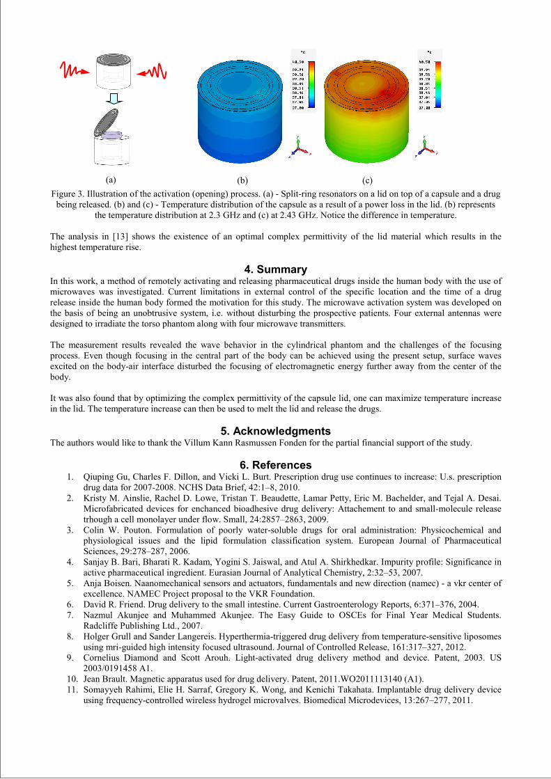
Figure 3. Illustration of the activation (opening) process. (a) - Split-ring resonators on a lid on top of a capsule and a drug
being released. (b) and (c) - Temperature distribution of the capsule as a result of a power loss in the lid. (b) represents the temperature distribution at 2.3 GHz and (c) at 2.43 GHz. Notice the difference in temperature.
The analysis in [13] shows the existence of an optimal complex permittivity of the lid material which results in the highest temperature rise.
4. Summary In this work, a method of remotely activating and releasing pharmaceutical drugs inside the human body with the use of microwaves was investigated. Current limitations in external control of the specific location and the time of a drug release inside the human body formed the motivation for this study. The microwave activation system was developed on the basis of being an unobtrusive system, i.e. without disturbing the prospective patients. Four external antennas were designed to irradiate the torso phantom along with four microwave transmitters. The measurement results revealed the wave behavior in the cylindrical phantom and the challenges of the focusing process. Even though focusing in the central part of the body can be achieved using the present setup, surface waves excited on the body-air interface disturbed the focusing of electromagnetic energy further away from the center of the body. It was also found that by optimizing the complex permittivity of the capsule lid, one can maximize temperature increase in the lid. The temperature increase can then be used to melt the lid and release the drugs.
5. Acknowledgments The authors would like to thank the Villum Kann Rasmussen Fonden for the partial financial support of the study.
6. References 1. Qiuping Gu, Charles F. Dillon, and Vicki L. Burt. Prescription drug use continues to increase: U.s. prescription
drug data for 2007-2008. NCHS Data Brief, 42:1–8, 2010. 2. Kristy M. Ainslie, Rachel D. Lowe, Tristan T. Beaudette, Lamar Petty, Eric M. Bachelder, and Tejal A. Desai.
Microfabricated devices for enchanced bioadhesive drug delivery: Attachement to and small-molecule release trhough a cell monolayer under flow. Small, 24:2857–2863, 2009.
3. Colin W. Pouton. Formulation of poorly water-soluble drugs for oral administration: Physicochemical and physiological issues and the lipid formulation classification system. European Journal of Pharmaceutical Sciences, 29:278–287, 2006.
4. Sanjay B. Bari, Bharati R. Kadam, Yogini S. Jaiswal, and Atul A. Shirkhedkar. Impurity profile: Significance in active pharmaceutical ingredient. Eurasian Journal of Analytical Chemistry, 2:32–53, 2007.
5. Anja Boisen. Naanomechanical sensors and actuators, fundamentals and new direction (namec) - a vkr center of excellence. NAMEC Project proposal to the VKR Foundation.
6. David R. Friend. Drug delivery to the small intestine. Current Gastroenterology Reports, 6:371–376, 2004. 7. Nazmul Akunjee and Muhammed Akunjee. The Easy Guide to OSCEs for Final Year Medical Students.
Radcliffe Publishing Ltd., 2007. 8. Holger Grull and Sander Langereis. Hyperthermia-triggered drug delivery from temperature-sensitive liposomes
using mri-guided high intensity focused ultrasound. Journal of Controlled Release, 161:317–327, 2012. 9. Cornelius Diamond and Scott Arouh. Light-activated drug delivery method and device. Patent, 2003. US
2003/0191458 A1. 10. Jean Brault. Magnetic apparatus used for drug delivery. Patent, 2011.WO2011113140 (A1). 11. Somayyeh Rahimi, Elie H. Sarraf, Gregory K. Wong, and Kenichi Takahata. Implantable drug delivery device
using frequency-controlled wireless hydrogel microvalves. Biomedical Microdevices, 13:267–277, 2011.
(a) (b) (c)

12. S. Smith, T.B. Tang, J.G. Terry, J.T.M. Stevenson, B.W. Flynn, H.M. Reekie, A.F. Murray, A.M. gundlach, D. Renshaw, B. Dhillon, A. Ohtori, Y. Inoue, and A.J. Walton. Development of a miniaturised drug delivery system with wireless power transfer and communication. IET Nanobiotechnology, 1:80–86, 2007.
13. Jónasson, Sævar Þór, Jensen, Brian Sveistrup, Johansen, Tom Keinicke, “Study of split-ring resonators for use on a pharmaceutical drug capsule for microwave activated drug release,” Proceedings of European Microwave Conference 2012, pp. 76-79.
59
Conference Paper 4 [CP4]
Vital Signs Detection Radar using LowIntermediate-Frequency Architecture and
Single-Sideband Transmission
Brian Sveistrup Jensen, Sævar Þór Jónasson,Thomas Jensen and Tom Keinicke Johansen
Conference: EuRAD 2012 Amsterdam
Published : Oct. 2012
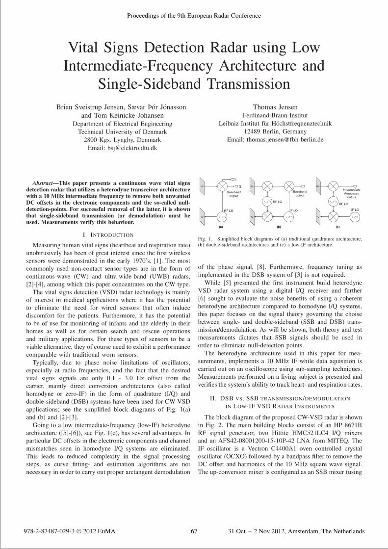
Vital Signs Detection Radar using LowIntermediate-Frequency Architecture and
Single-Sideband TransmissionBrian Sveistrup Jensen, Sævar Þór Jónasson
and Tom Keinicke JohansenDepartment of Electrical Engineering
Technical University of Denmark2800 Kgs. Lyngby, Denmark
Email: [email protected]
Thomas JensenFerdinand-Braun-Institut
Leibniz-Institut für Höchstfrequenztechnik12489 Berlin, Germany
Email: [email protected]
Abstract—This paper presents a continuous wave vital signsdetection radar that utilizes a heterodyne transceiver architecturewith a 10 MHz intermediate frequency to remove both unwantedDC offsets in the electronic components and the so-called null-detection-points. For successful removal of the latter, it is shownthat single-sideband transmission (or demodulation) must beused. Measurements verify this behaviour.
I. INTRODUCTION
Measuring human vital signs (heartbeat and respiration rate)unobtrusively has been of great interest since the first wirelesssensors were demonstrated in the early 1970’s, [1]. The mostcommonly used non-contact sensor types are in the form ofcontinuous-wave (CW) and ultra-wide-band (UWB) radars,[2]-[4], among which this paper concentrates on the CW type.
The vital signs detection (VSD) radar technology is mainlyof interest in medical applications where it has the potentialto eliminate the need for wired sensors that often inducediscomfort for the patients. Furthermore, it has the potentialto be of use for monitoring of infants and the elderly in theirhomes as well as for certain search and rescue operationsand military applications. For these types of sensors to be aviable alternative, they of course need to exhibit a performancecomparable with traditional worn sensors.
Typically, due to phase noise limitations of oscillators,especially at radio frequencies, and the fact that the desiredvital signs signals are only 0.1 - 3.0 Hz offset from thecarrier, mainly direct conversion architectures (also calledhomodyne or zero-IF) in the form of quadrature (I/Q) anddouble-sideband (DSB) systems have been used for CW-VSDapplications; see the simplified block diagrams of Fig. 1(a)and (b) and [2]-[3].
Going to a low intermediate-frequency (low-IF) heterodynearchitecture ([5]-[6]), see Fig. 1(c), has several advantages. Inparticular DC offsets in the electronic components and channelmismatches seen in homodyne I/Q systems are eliminated.This leads to reduced complexity in the signal processingsteps, as curve fitting- and estimation algorithms are notnecessary in order to carry out proper arctangent demodulation
TX
RX
Basebandoutput
TX
RX
Basebandoutput
TX
RXIntermediateFrequency
output
Fig. 1. Simplified block diagrams of (a) traditional quadrature architecture,(b) double-sideband architectures and (c) a low-IF architecture.
of the phase signal, [8]. Furthermore, frequency tuning asimplemented in the DSB system of [3] is not required.
While [5] presented the first instrument build heterodyneVSD radar system using a digital I/Q receiver and further[6] sought to evaluate the noise benefits of using a coherentheterodyne architecture compared to homodyne I/Q systems,this paper focuses on the signal theory governing the choisebetween single- and double-sideband (SSB and DSB) trans-mission/demodulation. As will be shown, both theory and testmeasurements dictates that SSB signals should be used inorder to eliminate null-detection points.
The heterodyne architecture used in this paper for mea-surements, implements a 10 MHz IF while data aquisition iscarried out on an oscilloscope using sub-sampling techniques.Measurements performed on a living subject is presented andverifies the system’s ability to track heart- and respiration rates.
II. DSB VS. SSB TRANSMISSION/DEMODULATIONIN LOW-IF VSD RADAR INSTRUMENTS
The block diagram of the proposed CW-VSD radar is shownin Fig. 2. The main building blocks consist of an HP 8671BRF signal generator, two Hittite HMC521LC4 I/Q mixersand an AFS42-08001200-15-10P-42 LNA from MITEQ. TheIF oscillator is a Vectron C4400A1 oven controlled crystaloscillator (OCXO) followed by a bandpass filter to remove theDC offset and harmonics of the 10 MHz square wave signal.The up-conversion mixer is configured as an SSB mixer (using
978-2-87487-029-3 © 2012 EuMA 31 Oct - 2 Nov 2012, Amsterdam, The Netherlands
Proceedings of the 9th European Radar Conference
67
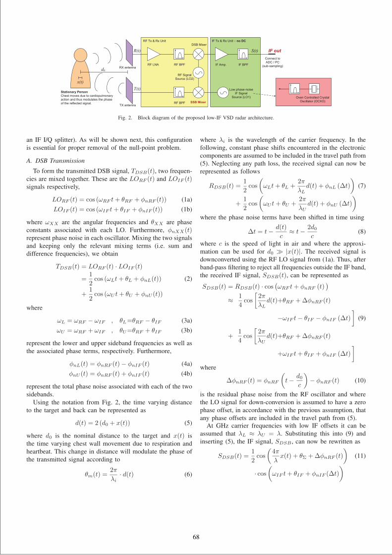
TX antenna
RX antenna
SSB Mixer
RF LNA
RF BPF
RF Tx & Rx Unit
Stationary PersonChest moves due to cardiopulmonary action and thus modulates the phase of the reflected signal.
Low phase-noise IF Signal
Source (LO1)
IF Amp.RF BPF IF BPF
IF Tx & Rx Unit – no DCDSB Mixer
RF Signal Source (LO2)
Connect toADC / PC
(sub-sampling)
Oven Controlled Crystal Oscillator (OCXO)
d0
x(t)T(t)
R(t) S(t)
Fig. 2. Block diagram of the proposed low-IF VSD radar architecture.
an IF I/Q splitter). As will be shown next, this configurationis essential for proper removal of the null-point problem.
A. DSB Transmission
To form the transmitted DSB signal, TDSB(t), two frequen-cies are mixed together. These are the LORF (t) and LOIF (t)signals respectively,
LORF (t) = cos (ωRF t+ θRF + φnRF (t)) (1a)LOIF (t) = cos (ωIF t+ θIF + φnIF (t)) (1b)
where ωXX are the angular frequencies and θXX are phaseconstants associated with each LO. Furthermore, φnXX(t)represent phase noise in each oscillator. Mixing the two signalsand keeping only the relevant mixing terms (i.e. sum anddifference frequencies), we obtain
TDSB(t) = LORF (t) · LOIF (t)
=1
2cos (ωLt+ θL + φnL(t)) (2)
+1
2cos (ωU t+ θU + φnU (t))
where
ωL = ωRF − ωIF , θL=θRF − θIF (3a)ωU = ωRF + ωIF , θU=θRF + θIF (3b)
represent the lower and upper sideband frequencies as well asthe associated phase terms, respectively. Furthermore,
φnL(t) = φnRF (t)− φnIF (t) (4a)φnU (t) = φnRF (t) + φnIF (t) (4b)
represent the total phase noise associated with each of the twosidebands.
Using the notation from Fig. 2, the time varying distanceto the target and back can be represented as
d(t) = 2 (d0 + x(t)) (5)
where d0 is the nominal distance to the target and x(t) isthe time varying chest wall movement due to respiration andheartbeat. This change in distance will modulate the phase ofthe transmitted signal according to
θm(t) =2π
λi· d(t) (6)
where λi is the wavelength of the carrier frequency. In thefollowing, constant phase shifts encountered in the electroniccomponents are assumed to be included in the travel path from(5). Neglecting any path loss, the received signal can now berepresented as follows
RDSB(t) =1
2cos
(ωLt+ θL +
2π
λLd(t) + φnL (Δt)
)(7)
+1
2cos
(ωU t+ θU +
2π
λUd(t) + φnU (Δt)
)
where the phase noise terms have been shifted in time using
Δt = t− d(t)
c≈ t− 2d0
c(8)
where c is the speed of light in air and where the approxi-mation can be used for d0 |x(t)|. The received signal isdownconverted using the RF LO signal from (1a). Thus, afterband-pass filtering to reject all frequencies outside the IF band,the received IF signal, SDSB(t), can be represented as
SDSB(t) = RDSB(t) · cos(ωRF t+ φnRF (t)
)
≈ 1
4cos
[2π
λLd(t)+θRF +ΔφnRF (t)
−ωIF t− θIF − φnIF (Δt)
](9)
+1
4cos
[2π
λUd(t)+θRF +ΔφnRF (t)
+ωIF t+ θIF + φnIF (Δt)
]
where
ΔφnRF (t) = φnRF
(t− d0
c
)− φnRF (t) (10)
is the residual phase noise from the RF oscillator and wherethe LO signal for down-conversion is assumed to have a zerophase offset, in accordance with the previous assumption, thatany phase offsets are included in the travel path from (5).
At GHz carrier frequencies with low IF offsets it can beassumed that λL ≈ λU = λ. Substituting this into (9) andinserting (5), the IF signal, SDSB , can now be rewritten as
SDSB(t) =1
2cos
(4π
λx(t) + θΣ +ΔφnRF (t)
)(11)
· cos(ωIF t+ θIF + φnIF (Δt)
)
68
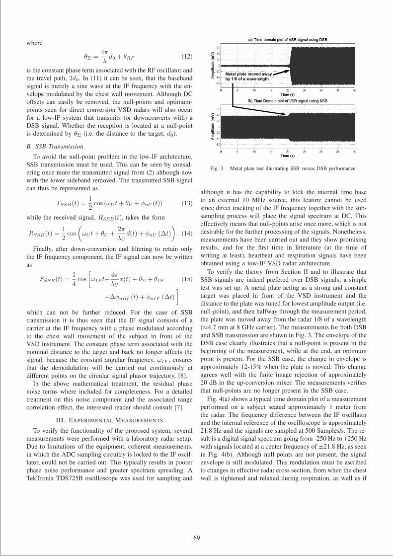
where
θΣ =4π
λd0 + θRF (12)
is the constant phase term associated with the RF oscillator andthe travel path, 2d0. In (11) it can be seen, that the basebandsignal is merely a sine wave at the IF frequency with the en-velope modulated by the chest wall movement. Although DCoffsets can easily be removed, the null-points and optimum-points seen for direct conversion VSD radars will also occurfor a low-IF system that transmits (or downconverts with) aDSB signal. Whether the reception is located at a null-pointis determined by θΣ (i.e. the distance to the target, d0).
B. SSB Transmission
To avoid the null-point problem in the low-IF architecture,SSB transmission must be used. This can be seen by consid-ering once more the transmitted signal from (2) although nowwith the lower sideband removed. The transmitted SSB signalcan thus be represented as
TSSB(t) =1
2cos (ωU t+ θU + φnU (t)) (13)
while the received signal, RSSB(t), takes the form
RSSB(t) =1
2cos
(ωU t+ θU +
2π
λUd(t) + φnU (Δt)
). (14)
Finally, after down-conversion and filtering to retain onlythe IF frequency component, the IF signal can now be writtenas
SSSB(t) =1
4cos
[ωIF t+
4π
λUx(t) + θΣ + θIF (15)
+ΔφnRF (t) + φnIF (Δt)
]
which can not be further reduced. For the case of SSBtransmission it is thus seen that the IF signal consists of acarrier at the IF frequency with a phase modulated accordingto the chest wall movement of the subject in front of theVSD instrument. The constant phase term associated with thenominal distance to the target and back no longer affects thesignal, because the constant angular frequency, ωIF , ensuresthat the demodulation will be carried out continuously atdifferent points on the circular signal phasor trajectory, [8].
In the above mathematical treatment, the residual phasenoise terms where included for completeness. For a detailedtreatment on this noise component and the associated rangecorrelation effect, the interested reader should consult [7].
III. EXPERIMENTAL MEASUREMENTS
To verify the functionality of the proposed system, severalmeasurements were performed with a laboratory radar setup.Due to limitations of the equipment, coherent measurements,in which the ADC sampling circuitry is locked to the IF oscil-lator, could not be carried out. This typically results in poorerphase noise performance and greater spectrum spreading. ATekTronix TDS725B oscilloscope was used for sampling and
Fig. 3. Metal plate test illustrating SSB versus DSB performance.
although it has the capability to lock the internal time baseto an external 10 MHz source, this feature cannot be usedsince direct tracking of the IF frequency together with the sub-sampling process will place the signal spectrum at DC. Thiseffectively means that null-points arise once more, which is notdesirable for the further processing of the signals. Nonetheless,measurements have been carried out and they show promisingresults, and for the first time in litterature (at the time ofwriting at least), heartbeat and respiration signals have beenobtained using a low-IF VSD radar architecture.
To verify the theory from Section II and to illustrate thatSSB signals are indeed prefered over DSB signals, a simpletest was set up. A metal plate acting as a strong and constanttarget was placed in front of the VSD instrument and thedistance to the plate was tuned for lowest amplitude output (i.e.null-point), and then halfway through the measurement period,the plate was moved away from the radar 1/8 of a wavelength(≈4.7 mm at 8 GHz carrier). The measurements for both DSBand SSB transmission are shown in Fig. 3. The envelope of theDSB case clearly illustrates that a null-point is present in thebeginning of the measurement, while at the end, an optimumpoint is present. For the SSB case, the change in envelope isapproximately 12-15% when the plate is moved. This changeagrees well with the finite image rejection of approximately20 dB in the up-conversion mixer. The measurements verifiesthat null-points are no longer present in the SSB case.
Fig. 4(a) shows a typical time domain plot of a measurementperformed on a subject seated approximately 1 meter fromthe radar. The frequency difference between the IF oscillatorand the internal reference of the oscilloscope is approximately21.8 Hz and the signals are sampled at 500 Samples/s. The re-sult is a digital signal spectrum going from -250 Hz to +250 Hzwith signals located at a center frequency of ±21.8 Hz, as seenin Fig. 4(b). Although null-points are not present, the signalenvelope is still modulated. This modulation must be ascribedto changes in effective radar cross section, from when the chestwall is tightened and relaxed during respiration, as well as if
69
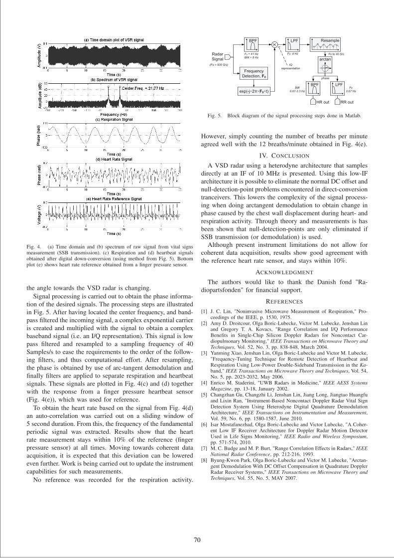
Fig. 4. (a) Time domain and (b) spectrum of raw signal from vital signsmeasurement (SSB transmission). (c) Respiration and (d) heartbeat signalsobtained after digital down-conversion (using method from Fig. 5). Bottomplot (e) shows heart rate reference obtained from a finger pressure sensor.
the angle towards the VSD radar is changing.Signal processing is carried out to obtain the phase informa-
tion of the desired signals. The processing steps are illustratedin Fig. 5. After having located the center frequency, and band-pass filtered the incoming signal, a complex exponential carrieris created and multiplied with the signal to obtain a complexbaseband signal (i.e. an I/Q representation). This signal is lowpass filtered and resampled to a sampling frequency of 40Samples/s to ease the requirements to the order of the follow-ing filters, and thus computational effort. After resampling,the phase is obtained by use of arc-tangent demodulation andfinally filters are applied to separate respiration and heartbeatsignals. These signals are plotted in Fig. 4(c) and (d) togetherwith the response from a finger pressure heartbeat sensor(Fig. 4(e)), which was used for reference.
To obtain the heart rate based on the signal from Fig. 4(d)an auto-correlation was carried out on a sliding window of5 second duration. From this, the frequency of the fundamentalperiodic signal was extracted. Results show that the heartrate measurement stays within 10% of the reference (fingerpressure sensor) at all times. Moving towards coherent dataacquisition, it is expected that this deviation can be loweredeven further. Work is being carried out to update the instrumentcapabilities for such measurements.
No reference was recorded for the respiration activity.
BPF
LPF
Resample
exp(-j×2 ×F0×t)
Frequency Detection, F0
BPF
LPF
Radar Signal
HR out RR out
F0 = 41 HzBW = 8 Hz
Fc: 4 Hz
BW0.67-3.3 Hz
Fc0.67 Hz
Fs to 40 S/s
(Fs = 500 S/s) IQrepresentation
arctan
phase
Fig. 5. Block diagram of the signal processing steps done in Matlab.
However, simply counting the number of breaths per minuteagreed well with the 12 breaths/minute obtained in Fig. 4(e).
IV. CONCLUSION
A VSD radar using a heterodyne architecture that samplesdirectly at an IF of 10 MHz is presented. Using this low-IFarchitecture it is possible to eliminate the normal DC offset andnull-detection-point problems encountered in direct-conversiontranceivers. This lowers the complexity of the signal process-ing when doing arctangent demodulation to obtain change inphase caused by the chest wall displacement during heart- andrespiration activity. Through theory and measurements is hasbeen shown that null-detection-points are only eliminated ifSSB transmission (or demodulation) is used.
Although present instrument limitations do not allow forcoherent data acquisition, results show good agreement withthe reference heart rate sensor, and stays within 10%.
ACKNOWLEDGMENT
The authors would like to thank the Danish fond "Ra-diopartsfonden" for financial support.
REFERENCES
[1] J. C. Lin, "Noninvasive Microwave Measurement of Respiration," Pro-ceedings of the IEEE, p. 1530, 1975.
[2] Amy D. Droitcour, Olga Boric-Lubecke, Victor M. Lubecke, Jenshan Linand Gregory T. A. Kovacs, "Range Correlation and I/Q PerformanceBenefits in Single-Chip Silicon Doppler Radars for Noncontact Car-diopulmonary Monitoring," IEEE Transactions on Microwave Theory andTechniques, Vol. 52, No. 3, pp. 838-848, March 2004.
[3] Yanming Xiao, Jenshan Lin, Olga Boric-Lubecke and Victor M. Lubecke,"Frequency-Tuning Technique for Remote Detection of Heartbeat andRespiration Using Low-Power Double-Sideband Transmission in the Ka-band," IEEE Transactions on Microwave Theory and Techniques, Vol. 54,No. 5, pp. 2023-2032, May 2006.
[4] Enrico M. Staderini, "UWB Radars in Medicine," IEEE AESS SystemsMagazine, pp. 13-18, January 2002.
[5] Changzhan Gu, Changzhi Li, Jenshan Lin, Jiang Long, Jiangtao Huangfuand Lixin Ran, "Instrument-Based Noncontact Doppler Radar Vital SignDetection System Using Heterodyne Digital Quadrature DemodulationArchitecture," IEEE Transactions on Instrumentation and Measurement,Vol. 59, No. 6, pp. 1580-1587, June 2010.
[6] Isar Mostafanezhad, Olga Boric-Lubecke and Victor Lubecke, "A Coher-ent Low IF Receiver Architecture for Doppler Radar Motion DetectorUsed in Life Signs Monitoring," IEEE Radio and Wireless Symposium,pp. 571-574, 2010.
[7] M. C. Budge and M. P. Burt, "Range Correlation Effects in Radars," IEEENational Radar Conference, pp. 212-216, 1993.
[8] Byung-Kwon Park, Olga Boric-Lubecke and Victor M. Lubecke, "Arctan-gent Demodulation With DC Offset Compensation in Quadrature DopplerRadar Receiver Systems," IEEE Transactions on Microwave Theory andTechniques, Vol. 55, No. 5, MAY 2007.
70

64
Conference Paper 5 [CP5]
Bondwire array modeling for the design ofhybrid high power amplifiers above C-band
Carlos Cilla Hernández, Sævar Þór Jónassonand Jesper Hanberg
Conference: Asia-Pacific Microwave Conference,Kaohsiung, Taiwan
Published : Dec. 2012
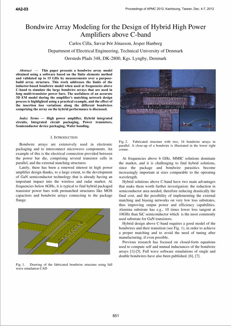
Bondwire Array Modeling for the Design of Hybrid High Power Amplifiers above C-band
Carlos Cilla, Sævar Þór Jónasson, Jesper Hanberg
Department of Electrical Engineering, Technical University of Denmark
Oersteds Plads 348, DK-2800, Kgs. Lyngby, Denmark
Abstract — This paper presents a bondwire array model
obtained using a software based on the finite elements method and validated up to 15 GHz by measurements over a purpose-build array structure. This work addresses the limits of the inductor-based bondwire model when used at frequencies above C-band to simulate the large bondwire arrays that are used in long multi-transistor power bars. The usefulness of an accurate 3D EM model during the amplifier’s matching network design process is highlighted using a practical example, and the effect of the insertion loss variations along the different bondwires comprising the array on the hybrid performance is discussed.
Index Terms — High power amplifier, Hybrid integrated circuits, Integrated circuit packaging, Power transistors, Semiconductor device packaging, Wafer bonding.
I. INTRODUCTION
Bondwire arrays are extensively used in electronic packaging and to interconnect microwave components. An example of this is the electrical connection provided between the power bar die, comprising several transistor cells in parallel, and the external matching structures.
Lately, there has been a renewed interest in high power amplifier design thanks, to a large extent, to the development of GaN semiconductor technology that is already having an important impact into the wireless and radar market. At frequencies below 6GHz, it is typical to find hybrid packaged transistor power bars with prematched structures like MOS capacitors and bondwire arrays connecting to the package flange.
Fig. 1. Drawing of the fabricated bondwire structure using full wave simulation CAD
Fig. 2. Fabricated structure with two, 16 bondwire arrays in parallel. A close-up of a bondwire is illustrated in the lower right corner.
At frequencies above 6 GHz, MMIC solutions dominate
the market, and it is challenging to find hybrid solutions, since the package and bondwire parasitics become increasingly important at sizes comparable to the operating wavelength.
Hybrid solutions above C-band have two main advantages that make them worth further investigation: the reduction in semiconductor area needed, therefore reducing drastically the final cost, and the possibility of implementing the external matching and biasing networks on very low loss substrates, thus improving output power and efficiency capabilities. Alumina substrate has e.g., 10 times lower loss tangent at 10GHz than SiC semiconductor which is the most commonly used substrate for GaN transistors.
Hybrid design above C-band requires a good model of the bondwires and their transition (see Fig. 1), in order to achieve a proper matching and to avoid the need of tuning after manufacturing, if even possible.
Previous research has focused on closed-form equations used to compute self and mutual inductances of the bondwire arrays [1]-[5]. Full wave software simulations of single and double bondwires have also been published. [6], [7].
851
4A2-034A2-034A2-034A2-03 Proceedings of APMC 2012, Kaohsiung, Taiwan, Dec. 4-7, 2012
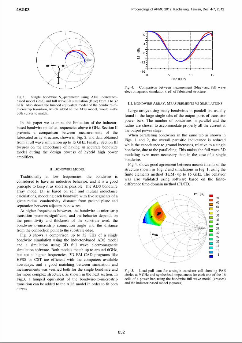
Fig.3. Single bondwire S11-parameter using ADS inductance- based model (Red) and full wave 3D simulation (Blue) from 1 to 32 GHz. Also shown the lumped equivalent model of the bondwire-to-microstrip transition, which added to the ADS model, would make both curves to match.
In this paper we examine the limitation of the inductor-based bondwire model at frequencies above 6 GHz. Section II presents a comparison between measurements of the fabricated array structure, shown in Fig. 2, and data obtained from a full wave simulation up to 15 GHz. Finally, Section III focuses on the importance of having an accurate bondwire model during the design process of hybrid high power amplifiers.
II. BONDWIRE MODEL
Traditionally at low frequencies, the bondwire is considered to have an inductive behavior, and it is a good principle to keep it as short as possible. The ADS bondwire array model [3] is based on self and mutual inductance calculations, modeling each bondwire with five segments of a given radius, conductivity, distance from ground plane and separation between adjacent bondwires.
At higher frequencies however, the bondwire-to-microstrip transition becomes significant, and the behavior depends on the permittivity and thickness of the substrate used, the bondwire-to-microstrip connection angle and the distance from the connection point to the substrate edge.
Fig. 3 shows a comparison up to 32 GHz of a single bondwire simulation using the inductor-based ADS model and a simulation using 3D full wave electromagnetic simulation software. Both models match up to around 6GHz, but not at higher frequencies. 3D EM CAD programs like HFSS or CST are efficient with the computers available nowadays, and a good matching between simulation and measurements was verified both for the single bondwire and for more complex structures, as shown in the next section. In Fig.3, a lumped equivalent of the bondwire-to-microstrip transition can be added to the ADS model in order to fit both curves.
Fig. 4. Comparison between measurement (blue) and full wave electromagnetic simulation (red) of fabricated structure.
III. BONDWIRE ARRAY: MEASUREMENTS VS SIMULATIONS
Large arrays using many bondwires in paralell are usually found in the large single tabs of the output ports of transistor power bars. The number of bondwires in parallel and the radius are chosen to accommodate properly all the current at the output power stage.
When paralleling bondwires in the same tab as shown in Figs. 1 and 2, the overall parasitic inductance is reduced while the capacitance to ground increases, relative to a single bondwire, due to the paralleling. This makes the full wave 3D modeling even more necessary than in the case of a single bondwire.
Fig 4. shows good agreement between measurements of the structure shown in Fig. 2 and simulations in Fig. 1, using the finite elements method (FEM) up to 15 GHz. The behavior was also validated using software based on the finite-difference time-domain method (FDTD).
Fig. 5. Load pull data for a single transistor cell showing PAE circles at 9 GHz and synthesized impedances for each one of the 16 cells of a power bar, using the bondwire full wave model (crosses) and the inductor-based model (squares)
852
4A2-034A2-034A2-034A2-03 Proceedings of APMC 2012, Kaohsiung, Taiwan, Dec. 4-7, 2012
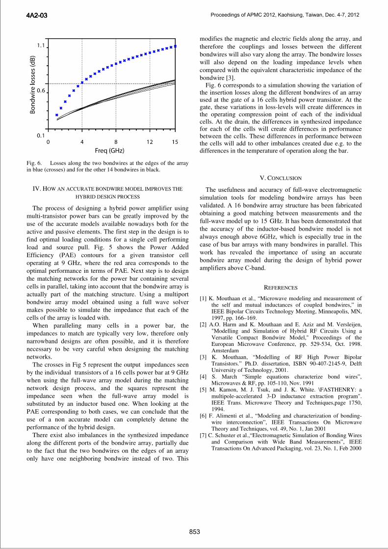
Fig. 6. Losses along the two bondwires at the edges of the array in blue (crosses) and for the other 14 bondwires in black.
IV. HOW AN ACCURATE BONDWIRE MODEL IMPROVES THE
HYBRID DESIGN PROCESS
The process of designing a hybrid power amplifier using multi-transistor power bars can be greatly improved by the use of the accurate models available nowadays both for the active and passive elements. The first step in the design is to find optimal loading conditions for a single cell performing load and source pull. Fig. 5 shows the Power Added Efficiency (PAE) contours for a given transistor cell operating at 9 GHz, where the red area corresponds to the optimal performance in terms of PAE. Next step is to design the matching networks for the power bar containing several cells in parallel, taking into account that the bondwire array is actually part of the matching structure. Using a multiport bondwire array model obtained using a full wave solver makes possible to simulate the impedance that each of the cells of the array is loaded with.
When paralleling many cells in a power bar, the impedances to match are typically very low, therefore only narrowband designs are often possible, and it is therefore necessary to be very careful when designing the matching networks.
The crosses in Fig 5 represent the output impedances seen by the individual transistors of a 16 cells power bar at 9 GHz when using the full-wave array model during the matching network design process, and the squares represent the impedance seen when the full-wave array model is substituted by an inductor based one. When looking at the PAE corresponding to both cases, we can conclude that the use of a non accurate model can completely detune the performance of the hybrid design.
There exist also imbalances in the synthesized impedance along the different ports of the bondwire array, partially due to the fact that the two bondwires on the edges of an array only have one neighboring bondwire instead of two. This
modifies the magnetic and electric fields along the array, and therefore the couplings and losses between the different bondwires will also vary along the array. The bondwire losses will also depend on the loading impedance levels when compared with the equivalent characteristic impedance of the bondwire [3].
Fig. 6 corresponds to a simulation showing the variation of the insertion losses along the different bondwires of an array used at the gate of a 16 cells hybrid power transistor. At the gate, these variations in loss-levels will create differences in the operating compression point of each of the individual cells. At the drain, the differences in synthesized impedance for each of the cells will create differences in performance between the cells. These differences in performance between the cells will add to other imbalances created due e.g. to the differences in the temperature of operation along the bar.
V. CONCLUSION
The usefulness and accuracy of full-wave electromagnetic simulation tools for modeling bondwire arrays has been validated. A 16 bondwire array structure has been fabricated obtaining a good matching between measurements and the full-wave model up to 15 GHz. It has been demonstrated that the accuracy of the inductor-based bondwire model is not always enough above 6GHz, which is especially true in the case of bus bar arrays with many bondwires in parallel. This work has revealed the importance of using an accurate bondwire array model during the design of hybrid power amplifiers above C-band.
REFERENCES
[1] K. Mouthaan et al., “Microwave modeling and measurement of the self and mutual inductances of coupled bondwires,” in IEEE Bipolar Circuits Technology Meeting, Minneapolis, MN, 1997, pp. 166–169.
[2] A.O. Harm and K. Mouthaan and E. Aziz and M. Versleijen, "Modelling and Simulation of Hybrid RF Circuits Using a Versatile Compact Bondwire Model," Proceedings of the European Microwave Conference, pp. 529-534, Oct. 1998. Amsterdam
[3] K. Mouthaan, “Modelling of RF High Power Bipolar Transistors.” Ph.D. dissertation, ISBN 90-407-2145-9, Delft University of Technology, 2001.
[4] S. March “Simple equations characterize bond wires”, Microwaves & RF, pp. 105-110, Nov. 1991
[5] M. Kamon, M. J. Tsuk, and J. K. White. \FASTHENRY: a multipole-accelerated 3-D inductance extraction program". IEEE Trans. Microwave Theory and Techniques,page 1750, 1994.
[6] F. Alimenti et al., “Modeling and characterization of bonding-wire interconnection”, IEEE Transactions On Microwave Theory and Techniques, vol. 49, No. 1, Jan 2001
[7] C. Schuster et al.,“Electromagnetic Simulation of Bonding Wires and Comparison with Wide Band Measurements”, IEEE Transactions On Advanced Packaging, vol. 23, No. 1, Feb 2000
853
4A2-034A2-034A2-034A2-03 Proceedings of APMC 2012, Kaohsiung, Taiwan, Dec. 4-7, 2012
68
Conference Paper 6 [CP6]
Cantilever-Based Microwave Biosensors:Analysis, Designs and Optimizations
Chenhui Jiang, Tom Keinicke Johansen,Sævar Þór Jónasson, Lei Yan and Anja Boisen
Conference:27th Annual Review of Progress in Ap-plied Computational Electromagnetics,Virginia, USA
Published : March 2011
Cantilever-based Microwave Biosensors: Analysis, Designs and Optimizations
Chenhui Jiang1, Tom K. Johansen
1, Sævar Þór Jónasson
1, Lei Yan
1 and Anja Boisen
2
1Department of Electrical Engineering
Technical University of Denmark, Kgs. Lyngby, 2800, Denmark
2Department of Micro- and Nanotechnology
Technical University of Denmark, Kgs. Lyngby, 2800, Denmark
Abstract: This paper presents a novel microwave readout scheme for measuring deflection of cantilevers
in nanometer range. The cantilever deflection can be sensed by the variation of transmission levels or
resonant frequencies of microwave signals. The sensitivity of the cantilever biosensor based on LC
resonators is at first theoretically analyzed. A LC resonator based biosensor with beams is designed and
optimized by using 3D electromagnetic (EM) simulations, where the beam is a typical variation of
cantilevers. The sensitivity of the lossless biosensor is predicted as 4.6MHz/nm. The 3-dB bandwidths of
the resonances are narrowed for improving the resolution of distinguishing resonances by reducing
conductive loss of electrodes. The lossy biosensor can achieve the highest sensitivity as 5.6 MHz/nm and
narrowest 3-dB bandwidth as 5 GHz.
Keywords: Cantilevers, beams, microwave biosensors, LC resonators, electromagnetic simulations,
1. Introduction
Biosensors have been widely used in identifying target molecular, recognizing a suitable biological
element, monitoring micro-environment parameters, developing drug discovery and targeted drug
delivery systems [1-4]. They are attracting numerous research and commercial interests due to these
applications. Cantilevers, which are micrometer sized diving boards, can be used as sensitive and versatile
label free biosensors [5]. The cantilever based sensors exhibit merits in the aspect of label-free usage,
high sensitivity, portability, low cost and highly parallel and fast responsibility. The cantilever may
deflect due to changes in temperature, surface stress and mass, which are major concerned parameters for
biosensing [5]. The cantilever-based biosensors can measure these parameters due to deflections of
cantilevers by several read-out principles. However, current read-out methods always have their
limitations. For example, the optical read-out [6, 7] is difficult to apply for large arrays and not suitable
for nanometer sized cantilevers. Even though piezoresistive read-out [8, 9] is suitable for large arrays and
system integration, a piezoresistive layer needs to be integrated into the cantilever so that it affects the
mechanical performance.
In order to overcome these limitations, microwave readout is proposed to detect cantilever deflections.
It is feasible to be applied in a single cantilever or a large array of cantilevers. Microwave electrodes are
easily integrated with operational cantilevers, and can act as an active layer on cantilevers as well.
Moreover microwave read-out scheme provides a possibility to approach lab-on-a-chip due to the full
integration sensor implementation and realize wireless sensing manners. Biosensors probed with
microwave, millimeter-wave or terahertz signals have been recently proposed by several groups [10-12].
These activities employ either split-ring resonators (SRRs) or Goubau lines (G-lines) [13] as sensing
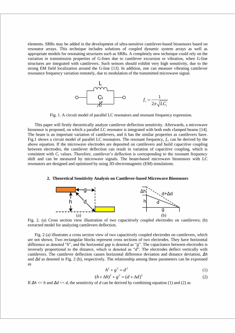
elements. SRRs may be added in the development of ultra-sensitive cantilever-based biosensors based on
resonator arrays. This technique includes solutions of coupled dynamic system arrays as well as
appropriate models for resonating structures such as SRRs. A completely new technique could rely on the
variation in transmission properties of G-lines due to cantilever excursion or vibration, when G-line
structures are integrated with cantilevers. Such sensors should exhibit very high sensitivity, due to the
strong EM field localization around the G-line [13]. In addition, one can measure vibrating cantilever
resonance frequency variation remotely, due to modulation of the transmitted microwave signal.
1
2r
t
fLC
Fig. 1. A circuit model of parallel LC resonators and resonant frequency expression.
This paper will firstly theoretically analyze cantilever deflection sensitivity. Afterwards, a microwave
biosensor is proposed, on which a parallel LC resonator is integrated with both ends clamped beams [14].
The beam is an important variation of cantilevers, and it has the similar properties as cantilevers have.
Fig.1 shows a circuit model of parallel LC resonators. The resonant frequency, fr, can be derived by the
above equation. If the microwave electrodes are deposited on cantilevers and build capacitive coupling
between electrodes, the cantilever deflection can result in variation of capacitive coupling, which is
consistent with Ct values. Therefore, cantilever’s deflection is corresponding to the resonant frequency
shift and can be measured by microwave signals. The beam-based microwave biosensors with LC
resonators are designed and optimized by using 3D electromagnetic (EM) simulations.
2. Theoretical Sensitivity Analysis on Cantilever-based Microwave Biosensors
(a) (b)
Fig. 2. (a) Cross section view illustration of two capacitively coupled electrodes on cantilevers; (b)
extracted model for analyzing cantilevers deflection.
Fig. 2 (a) illustrates a cross section view of two capacitively coupled electrodes on cantilevers, which
are not shown. Two rectangular blocks represent cross sections of two electrodes. They have horizontal
difference as denoted “h”, and the horizontal gap is denoted as “g”. The capacitance between electrodes is
inversely proportional to the distance, which is denoted as “d”. The electrodes deflect vertically with
cantilevers. The cantilever deflection causes horizontal difference deviation and distance deviation, Δh
and Δd as denoted in Fig. 2 (b), respectively. The relationship among these parameters can be expressed
as 2 2 2h g d (1)
2 2 2( ) ( )h h g d d (2)
If Δh << h and Δd << d, the sensitivity of d can be derived by combining equation (1) and (2) as
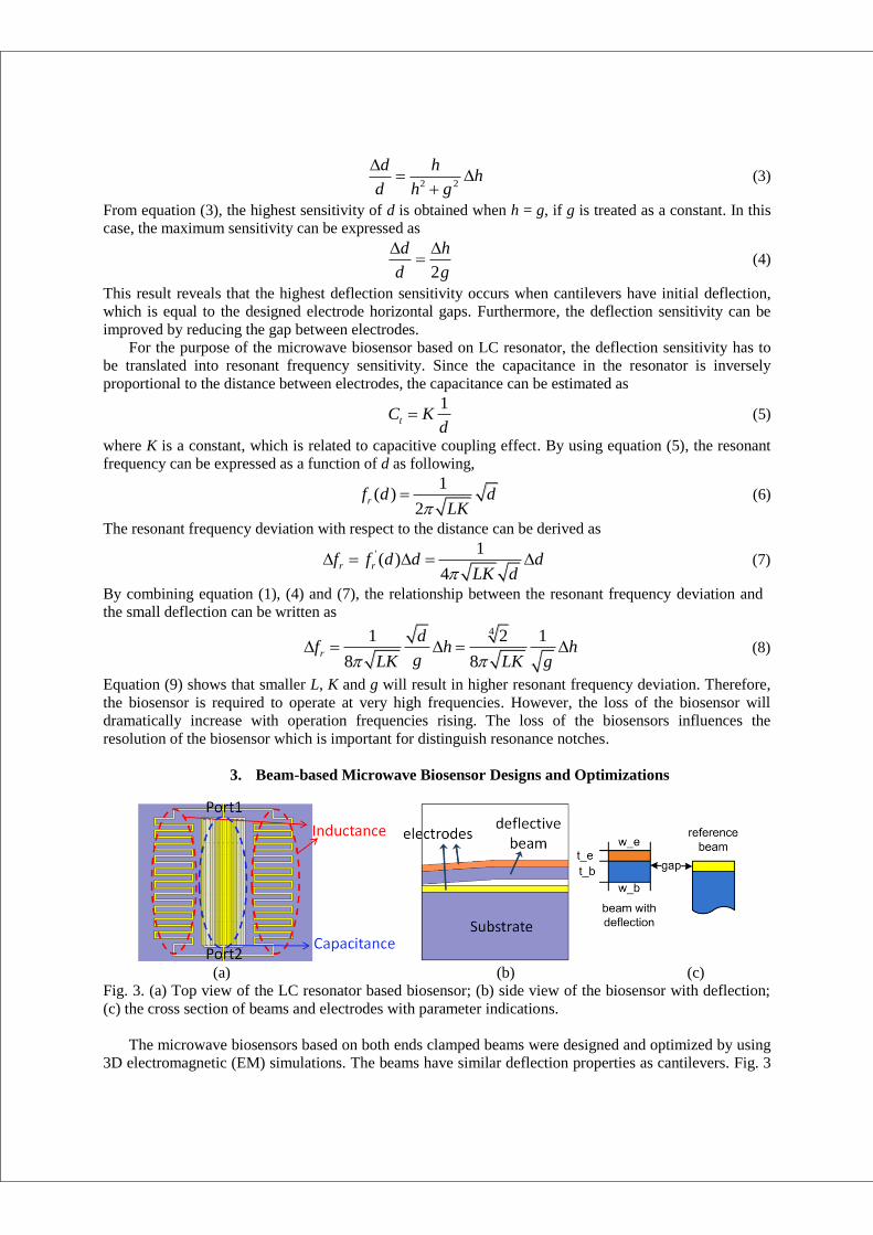
2 2
d hh
d h g
(3)
From equation (3), the highest sensitivity of d is obtained when h = g, if g is treated as a constant. In this
case, the maximum sensitivity can be expressed as
2
d h
d g
(4)
This result reveals that the highest deflection sensitivity occurs when cantilevers have initial deflection,
which is equal to the designed electrode horizontal gaps. Furthermore, the deflection sensitivity can be
improved by reducing the gap between electrodes.
For the purpose of the microwave biosensor based on LC resonator, the deflection sensitivity has to
be translated into resonant frequency sensitivity. Since the capacitance in the resonator is inversely
proportional to the distance between electrodes, the capacitance can be estimated as
1tC K
d (5)
where K is a constant, which is related to capacitive coupling effect. By using equation (5), the resonant
frequency can be expressed as a function of d as following,
1( )
2rf d d
LK (6)
The resonant frequency deviation with respect to the distance can be derived as
' 1( )
4r rf f d d d
LK d (7)
By combining equation (1), (4) and (7), the relationship between the resonant frequency deviation and
the small deflection can be written as 41 2 1
8 8r
df h h
gLK LK g (8)
Equation (9) shows that smaller L, K and g will result in higher resonant frequency deviation. Therefore,
the biosensor is required to operate at very high frequencies. However, the loss of the biosensor will
dramatically increase with operation frequencies rising. The loss of the biosensors influences the
resolution of the biosensor which is important for distinguish resonance notches.
3. Beam-based Microwave Biosensor Designs and Optimizations
(a) (b) (c)
Fig. 3. (a) Top view of the LC resonator based biosensor; (b) side view of the biosensor with deflection;
(c) the cross section of beams and electrodes with parameter indications.
The microwave biosensors based on both ends clamped beams were designed and optimized by using
3D electromagnetic (EM) simulations. The beams have similar deflection properties as cantilevers. Fig. 3
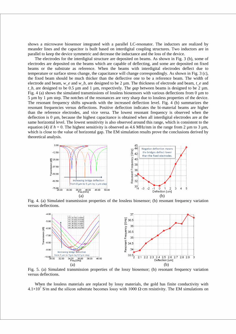
shows a microwave biosensor integrated with a parallel LC-resonator. The inductors are realized by
meander lines and the capacitor is built based on interdigital coupling structures. Two inductors are in
parallel to keep the device symmetric and decrease the inductance and the loss of the device.
The electrodes for the interdigital structure are deposited on beams. As shown in Fig. 3 (b), some of
electrodes are deposited on the beams which are capable of deflecting, and some are deposited on fixed
beams or the substrate as reference. When the beams with interdigital electrodes deflect due to
temperature or surface stress change, the capacitance will change correspondingly. As shown in Fig. 3 (c),
the fixed beam should be much thicker than the deflective one to be a reference beam. The width of
electrode and beam, w_e and w_b, are designed to be 2 µm. The thickness of electrode and beam, t_e and
t_b, are designed to be 0.5 µm and 1 µm, respectively. The gap between beams is designed to be 2 µm.
Fig. 4 (a) shows the simulated transmissions of lossless biosensors with various deflections from 0 µm to
5 µm by 1 µm step. The notches of the resonances are very sharp due to lossless properties of the device.
The resonant frequency shifts upwards with the increased deflection level. Fig. 4 (b) summarizes the
resonant frequencies versus deflections. Positive deflection indicates the bi-material beams are higher
than the reference electrodes, and vice versa. The lowest resonant frequency is observed when the
deflection is 0 µm, because the highest capacitance is obtained when all interdigital electrodes are at the
same horizontal level. The lowest sensitivity is also observed around this range, which is consistent to the
equation (4) if h = 0. The highest sensitivity is observed as 4.6 MHz/nm in the range from 2 µm to 3 µm,
which is close to the value of horizontal gap. The EM simulation results prove the conclusions derived by
theoretical analysis.
(a) (b)
Fig. 4. (a) Simulated transmission properties of the lossless biosensor; (b) resonant frequency variation
versus deflections.
(a) (b)
Fig. 5. (a) Simulated transmission properties of the lossy biosensor; (b) resonant frequency variation
versus deflections.
When the lossless materials are replaced by lossy materials, the gold has finite conductivity with
4.1×10⁷ S/m and the silicon substrate becomes lossy with 1000 Ω∙cm resistivity. The EM simulations on
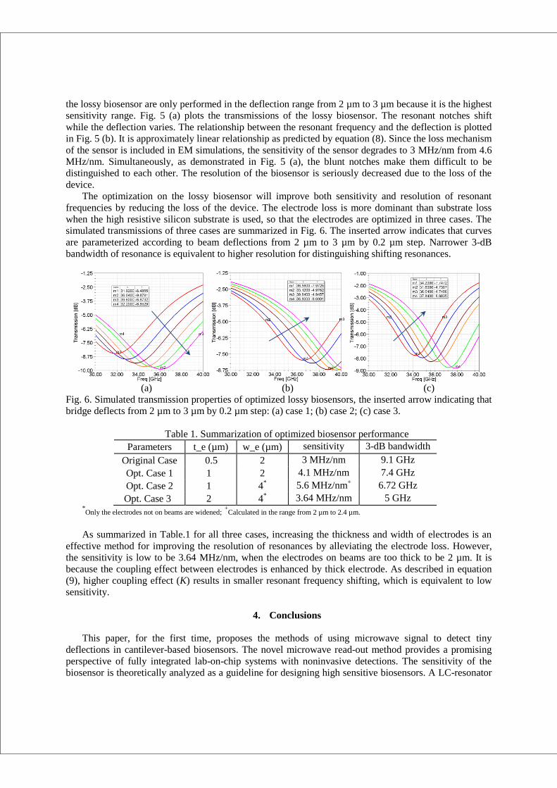
the lossy biosensor are only performed in the deflection range from 2 µm to 3 µm because it is the highest
sensitivity range. Fig. 5 (a) plots the transmissions of the lossy biosensor. The resonant notches shift
while the deflection varies. The relationship between the resonant frequency and the deflection is plotted
in Fig. 5 (b). It is approximately linear relationship as predicted by equation (8). Since the loss mechanism
of the sensor is included in EM simulations, the sensitivity of the sensor degrades to 3 MHz/nm from 4.6
MHz/nm. Simultaneously, as demonstrated in Fig. 5 (a), the blunt notches make them difficult to be
distinguished to each other. The resolution of the biosensor is seriously decreased due to the loss of the
device.
The optimization on the lossy biosensor will improve both sensitivity and resolution of resonant
frequencies by reducing the loss of the device. The electrode loss is more dominant than substrate loss
when the high resistive silicon substrate is used, so that the electrodes are optimized in three cases. The
simulated transmissions of three cases are summarized in Fig. 6. The inserted arrow indicates that curves
are parameterized according to beam deflections from 2 µm to 3 µm by 0.2 µm step. Narrower 3-dB
bandwidth of resonance is equivalent to higher resolution for distinguishing shifting resonances.
(a) (b) (c)
Fig. 6. Simulated transmission properties of optimized lossy biosensors, the inserted arrow indicating that
bridge deflects from 2 µm to 3 µm by 0.2 µm step: (a) case 1; (b) case 2; (c) case 3.
Table 1. Summarization of optimized biosensor performance
Parameters t_e (µm) w_e (µm) sensitivity 3-dB bandwidth
Original Case 0.5 2 3 MHz/nm 9.1 GHz
Opt. Case 1 1 2 4.1 MHz/nm 7.4 GHz
Opt. Case 2 1 4* 5.6 MHz/nm
+ 6.72 GHz
Opt. Case 3 2 4* 3.64 MHz/nm 5 GHz
*Only the electrodes not on beams are widened;
+Calculated in the range from 2 µm to 2.4 µm.
As summarized in Table.1 for all three cases, increasing the thickness and width of electrodes is an
effective method for improving the resolution of resonances by alleviating the electrode loss. However,
the sensitivity is low to be 3.64 MHz/nm, when the electrodes on beams are too thick to be 2 µm. It is
because the coupling effect between electrodes is enhanced by thick electrode. As described in equation
(9), higher coupling effect (K) results in smaller resonant frequency shifting, which is equivalent to low
sensitivity.
4. Conclusions
This paper, for the first time, proposes the methods of using microwave signal to detect tiny
deflections in cantilever-based biosensors. The novel microwave read-out method provides a promising
perspective of fully integrated lab-on-chip systems with noninvasive detections. The sensitivity of the
biosensor is theoretically analyzed as a guideline for designing high sensitive biosensors. A LC-resonator
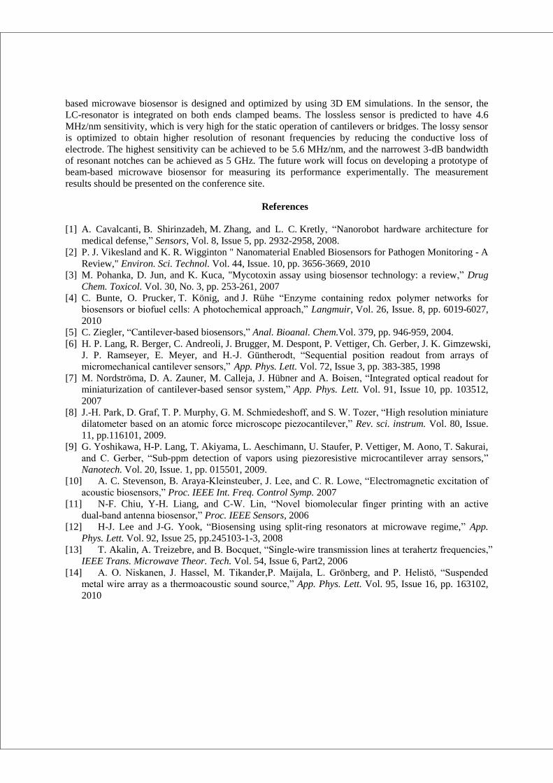
based microwave biosensor is designed and optimized by using 3D EM simulations. In the sensor, the
LC-resonator is integrated on both ends clamped beams. The lossless sensor is predicted to have 4.6
MHz/nm sensitivity, which is very high for the static operation of cantilevers or bridges. The lossy sensor
is optimized to obtain higher resolution of resonant frequencies by reducing the conductive loss of
electrode. The highest sensitivity can be achieved to be 5.6 MHz/nm, and the narrowest 3-dB bandwidth
of resonant notches can be achieved as 5 GHz. The future work will focus on developing a prototype of
beam-based microwave biosensor for measuring its performance experimentally. The measurement
results should be presented on the conference site.
References
[1] A. Cavalcanti, B. Shirinzadeh, M. Zhang, and L. C. Kretly, “Nanorobot hardware architecture for
medical defense,” Sensors, Vol. 8, Issue 5, pp. 2932-2958, 2008.
[2] P. J. Vikesland and K. R. Wigginton " Nanomaterial Enabled Biosensors for Pathogen Monitoring - A
Review," Environ. Sci. Technol. Vol. 44, Issue. 10, pp. 3656-3669, 2010
[3] M. Pohanka, D. Jun, and K. Kuca, "Mycotoxin assay using biosensor technology: a review,” Drug
Chem. Toxicol. Vol. 30, No. 3, pp. 253-261, 2007
[4] C. Bunte, O. Prucker, T. König, and J. Rühe “Enzyme containing redox polymer networks for
biosensors or biofuel cells: A photochemical approach,” Langmuir, Vol. 26, Issue. 8, pp. 6019-6027,
2010
[5] C. Ziegler, “Cantilever-based biosensors,” Anal. Bioanal. Chem.Vol. 379, pp. 946-959, 2004.
[6] H. P. Lang, R. Berger, C. Andreoli, J. Brugger, M. Despont, P. Vettiger, Ch. Gerber, J. K. Gimzewski,
J. P. Ramseyer, E. Meyer, and H.-J. Güntherodt, “Sequential position readout from arrays of
micromechanical cantilever sensors,” App. Phys. Lett. Vol. 72, Issue 3, pp. 383-385, 1998
[7] M. Nordströma, D. A. Zauner, M. Calleja, J. Hübner and A. Boisen, “Integrated optical readout for
miniaturization of cantilever-based sensor system,” App. Phys. Lett. Vol. 91, Issue 10, pp. 103512,
2007
[8] J.-H. Park, D. Graf, T. P. Murphy, G. M. Schmiedeshoff, and S. W. Tozer, “High resolution miniature
dilatometer based on an atomic force microscope piezocantilever,” Rev. sci. instrum. Vol. 80, Issue.
11, pp.116101, 2009.
[9] G. Yoshikawa, H-P. Lang, T. Akiyama, L. Aeschimann, U. Staufer, P. Vettiger, M. Aono, T. Sakurai,
and C. Gerber, “Sub-ppm detection of vapors using piezoresistive microcantilever array sensors,”
Nanotech. Vol. 20, Issue. 1, pp. 015501, 2009.
[10] A. C. Stevenson, B. Araya-Kleinsteuber, J. Lee, and C. R. Lowe, “Electromagnetic excitation of
acoustic biosensors,” Proc. IEEE Int. Freq. Control Symp. 2007
[11] N-F. Chiu, Y-H. Liang, and C-W. Lin, “Novel biomolecular finger printing with an active
dual-band antenna biosensor,” Proc. IEEE Sensors, 2006
[12] H-J. Lee and J-G. Yook, “Biosensing using split-ring resonators at microwave regime,” App.
Phys. Lett. Vol. 92, Issue 25, pp.245103-1-3, 2008
[13] T. Akalin, A. Treizebre, and B. Bocquet, “Single-wire transmission lines at terahertz frequencies,”
IEEE Trans. Microwave Theor. Tech. Vol. 54, Issue 6, Part2, 2006
[14] A. O. Niskanen, J. Hassel, M. Tikander,P. Maijala, L. Grönberg, and P. Helistö, “Suspended
metal wire array as a thermoacoustic sound source,” App. Phys. Lett. Vol. 95, Issue 16, pp. 163102,
2010

www.elektro.dtu.dk Department of Electrical Engineering
Electromagnetic Systems Group (EMS) Technical University of Denmark Ørsteds Plads Building 348 DK-2800 Kgs. Lyngby Denmark Tel: (+45) 45 25 38 00 Fax: (+45) 45 93 16 34 Email: [email protected]
ISBN XX-XXXXX-XX-X