Embed Size (px)
Citation preview
244 Int. J. Oil, Gas and Coal Technology, Vol. 4, No. 3, 2011
Copyright © 2011 Inderscience Enterprises Ltd.
Historical pipeline construction cost analysis
Zhenhua Rui*
Department of Mining and Geological Engineering,
University of Alaska Fairbanks,
Duckering Building 418, P.O. Box 750708,
Fairbanks, Alaska 99775, USA
Fax: +1-907-474-6635
E-mail: [email protected]
*Corresponding author
Paul A. Metz
Department of Mining and Geological Engineering,
University of Alaska Fairbanks,
Duckering Building 313, P.O. Box 755800,
Fairbanks, Alaska 99775, USA
Fax: +1-907-474-6635
E-mail: [email protected]
Doug B. Reynolds
School of Management,
University of Alaska Fairbanks,
P.O. Box 756080, Fairbanks, Alaska 99775, USA
Fax: +1-907-474-5219
E-mail: [email protected]
Gang Chen
Department of Mining and Geological Engineering,
University of Alaska Fairbanks,
Duckering Building 315, P.O. Box 755880,
Fairbanks, Alaska 99775, USA
Fax: +1-907-474-6635
E-mail: [email protected]
Xiyu Zhou
School of Management,
University of Alaska Fairbanks,
P.O. Box 756080, Fairbanks, Alaska 99775, USA
Fax: +1-907-474-5219
E-mail: [email protected]
Historical pipeline construction cost analysis 245
Abstract: This study aims to provide a reference for the pipeline construction cost, by analysing individual pipeline cost components with historical pipeline cost data. Cost data of 412 pipelines recorded between 1992 and 2008 in the Oil and Gas Journal are collected and adjusted to 2008 dollars with the chemical engineering plant cost index (CEPCI). The distribution and share of these 412 pipeline cost components are assessed based on pipeline diameter, pipeline length, pipeline capacity, the year of completion, locations of pipelines. The share of material and labour cost dominates the pipeline construction cost, which is about 71% of the total cost. In addition, the learning curve analysis is conducted to attain learning rate with respect to pipeline material and labour costs for different groups. Results show that learning rate and construction cost are varied by pipeline diameters, pipeline lengths, locations of pipelines and other factors. This study also investigates the causes of pipeline construction cost differences among different groups. [Received: October 13, 2010; Accepted: December 20, 2010]
Keywords: pipeline cost; cost analysis; distribution; learning curve; cost difference.
Reference to this paper should be made as follows: Rui, Z., Metz, P.A., Reynolds, D., Chen, G. and Zhou, X. (2011) ‘Historical pipeline construction cost analysis’, Int. J. Oil, Gas and Coal Technology, Vol. 4, No. 3, pp.244–263.
Biographical notes: Zhenhua Rui is a PhD student in Energy Engineering Management at the University of Alaska Fairbanks. He also received his Masters in Petroleum Engineering from the same university, in addition to a Masters in Geophysics from China University of Petroleum (Beijing). His current research is the engineering economics of the Alaska in-state natural gas pipeline.
Paul A. Metz is a Professor of Department of Mining and Geological Engineering at the University of Alaska Fairbanks. He received his PhD from Imperial College of Science Technology and Medicine, and MS in Economic Geology and MBA from the University of Alaska. His research interests include: market and transportation analysis of mineral resources; analysis of transport systems; engineering geological mapping and site investigation; and mineral and energy resource evaluation.
Doug B. Reynolds is a Professor of School of Management at the University of Alaska Fairbanks. He received his PhD from the University of New Mexico. His research interests include oil production and energy economics. Some of his papers include an explanation of how one energy resource can subsidise the cost of an alternative energy resource and how an energy theory of value can be approximated by defining energy grades for energy resources.
Gang Chen is a Professor of Department of Mining and Geological Engineering at the University of Alaska Fairbanks. He received his PhD in Mining Engineering from Virginia Polytechnic Institute and State University; He received his MS in Mining Engineering from the Colorado School of Mines. His research interests include: rock mechanics in mining and civil engineering; mine ground engineering; frozen ground engineering and GIS application in mining industry.
Xiyu Zhou is an Associate Professor of Finance at the School of Management of the University of Alaska Fairbanks. He received his PhD of Business Administration (Finance) from the University of North Carolina. He also
246 Z. Rui et al.
received MS in Economics from the University of Lausanne and MBA from China Europe International Business School respectively. His current research interests include: merger and acquisition, corporate governance and real estate mutual funds.
1 Introduction
Pipelining is an important and economical method to transport large quantities of oil and
natural gas in the petroleum industry. The first pipeline in the USA, two-inch in diameter
and over 8 km long, was built in 1865 (Scheduble, 2002). By 2008, US had a total of
793,285 km of pipelines, among which 244,620 km was for petroleum product and
548,685 km was for natural gas (Central Intelligence Agency, 2008). Historical pipeline
cost data have been analysed and used to estimate the construction costs for the different
types of pipeline cost by various researchers. Parker (2004) used natural gas transmission
pipeline costs to estimate hydrogen pipeline cost with the linear regression method.
Zhao (2000) analysed the diffusion, costs and learning curve in the development of
international gas transmission lines. Heddle et al. (2003) derived a multiple linear
regression model to estimate the CO2 pipeline construction cost. McCoy and Rubin
(2008) developed multiple non-linear regression models to forecast CO2 pipeline cost.
Pipeline cost was compared to LNG and GTL cost as supply options (Gandoolphe et al.,
2003). Zhang et al. (2007) calculated share of material cost using pipeline cost between
1993 and 2004 and indicated that share of material cost is constant for the same diameter
pipelines. The Oil and Gas Journal annually analysed estimated and actual pipeline cost
and forecasts trends for the next year (PennWell Corporation, 1992, 2009). Various
studies on pipeline cost have been conducted by different researchers in different
perspectives.
The purpose of this paper is to conduct a comprehensive analysis on pipeline costs
from 1992 to 2008 with various perspectives: the distribution of pipelines, shares of
pipeline cost components and learning-by-doing in pipeline construction. A number of
data processing and statistical descriptions are applied to the historical data. Causes of
cost differences and learning rate differences are also investigated.
2 Data sources and cost adjusting factors
2.1 Data sources
In this study, the pipelines are selected on the basis of data availability. Pipeline cost data
are collected from Federal Energy Regulatory Commission filing by gas transmission
companies, which are published in the Oil and Gas Journal annual data book (PennWell
Corporation, 1992, 2009). Due to limited offshore pipeline data, only onshore pipelines
are collected, and the pipeline cost in this paper does not include compressor station cost.
The pipeline dataset includes year of completion, pipeline diameters, pipeline lengths,
location of pipelines, and costs of pipeline cost components. Pipelines in the dataset were
distributed in all states in the USA (Alaska and Hawaii are excluded). The dataset also
contains the cost information of 15 Canadian pipelines. The pipelines were completed
Historical pipeline construction cost analysis 247
between 1992 and 2008. Unfortunately, the data did not show the construction period.
Therefore, cost is defined as real, accounted costs determined at the time of completion.
All pipeline construction component cost are reported in US dollar. The entire dataset has
412 observations of onshore pipelines. The five pipeline cost components are: material,
labour, miscellaneous, right of way (ROW) and total cost. Material cost is the cost of line
pipe, pipeline coating and cathodic protection. Labour cost consists of the cost of pipeline
construction labour. Miscellaneous cost is a composite of the costs of surveying,
engineering, supervision, contingencies, telecommunications equipment, freight, taxes,
allowances for funds used during construction, administration and overheads, and
regulatory filing fees. ROW cost contains the cost of ROW and allowance for damages.
The total cost is the sum of material cost, labour cost, miscellaneous cost and ROW cost
(PennWell Corporation, 1992, 2009).
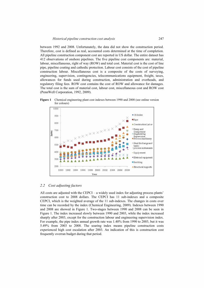
Figure 1 Chemical engineering plant cost indexes between 1990 and 2008 (see online version for colours)
2.2 Cost adjusting factors
All costs are adjusted with the CEPCI – a widely used index for adjusting process plants’
construction cost to 2008 dollars. The CEPCI has 11 sub-indexes and a composite
CEPCI, which is the weighted average of the 11 sub-indexes. The changes in costs over
time can be recorded by the index (Chemical Engineering, 2009). Indexes between 1990
and 2008 are showed in Figure 1. Two-stages between 1990 and 2008 can be seen in
Figure 1. The index increased slowly between 1990 and 2003, while the index increased
sharply after 2003, except for the construction labour and engineering supervision index.
For example, the pipe index annual growth rate was 1.40% from 1990 to 2003, but it was
5.49% from 2003 to 2008. The soaring index means pipeline construction costs
experienced high cost escalation after 2003. An indication of this is construction cost
frequently overran budget during that period.
248 Z. Rui et al.
The annual average growth rate between 1990 and 2008 is shown in Table 1. The
structure support index has the highest average annual growth rate of 4.09%. Engineering
supervision index is almost constant with the lowest average annual growth rate of
–0.04%. Pipe index average annual growth rate is 3.02% which is higher than the CE
index average annual growth rate of 2.54%. The index is a useful tool to adjust pipeline
cost data. To make cost data comparable to each other at the same base, different pipeline
cost components are adjusted by different indexes to 2008 dollars. Pipe index and
construction labour index is used to adjust pipeline material and labour cost. CE index is
applied to pipeline miscellaneous and ROW costs.
Table 1 Annual average growth rate of the chemical engineering plant cost index
Index type Annual growth rate Index type Annual growth rate
CE index 2.54% Heat exchange and tanks 3.30%
Pipe 3.02% Process instruments 1.10%
Construction labour 0.90% Equipment 3.07%
Pump and compressor 2.94% Electrical equipment 2.31%
Engineering supervision –0.04% Buildings 2.29%
Process machinery 3.01% Structural supports 4.09%
3 Data descriptive statistics
In order to better understand pipeline cost, the cost data of pipelines are analysed and
summarised in terms of pipeline diameters, pipeline length, pipeline capacity, year of
completion and location.
3.1 The distribution analysis of pipelines on year of completion, pipeline diameters and pipeline lengths
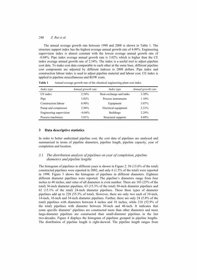
The histogram of pipelines in different years is shown in Figure 2. 56 (13.6% of the total)
constructed pipelines were reported in 2002, and only 6 (1.5% of the total) were reported
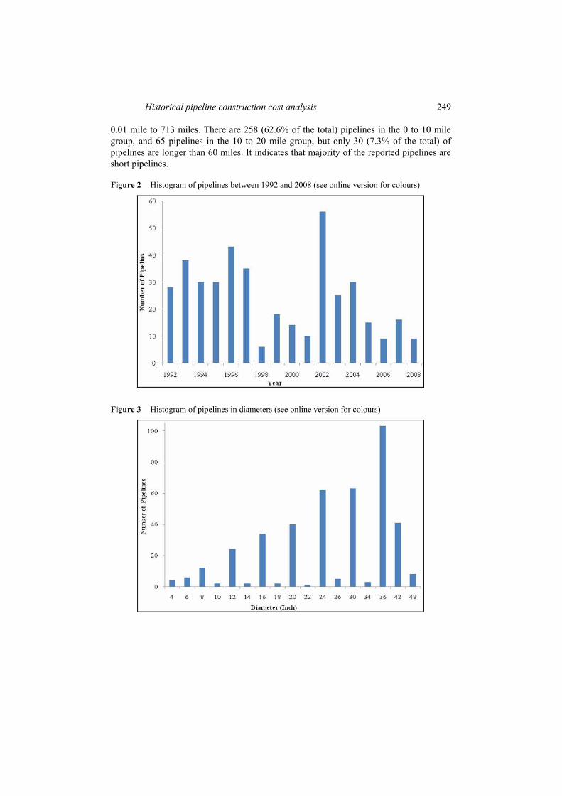
in 1998. Figure 3 shows the histogram of pipelines in different diameters. Eighteen
different diameter pipelines were reported. The pipeline’s diameters range from four
inches to 48 inches, and value of all diameters is even number. There are 103 (25% of the
total) 36-inch diameter pipelines, 63 (15.3% of the total) 30-inch diameter pipelines and
62 (15.1% of the total) 24-inch diameter pipelines. These three types of diameter
pipelines add up to 228 (55.3% of total). However, there are only two each of 10-inch,
14-inch, 18-inch and 34-inch diameter pipelines. Further, there are only 24 (5.8% of the
total) pipelines with diameters between 4 inches and 10 inches, while 218 (52.9% of
the total) pipelines with diameter between 30-inch and 48-inch. It indicates that
some specific diameter’ pipelines are constructed more than other diameters and more
large-diameter pipelines are constructed than small-diameter pipelines in the last
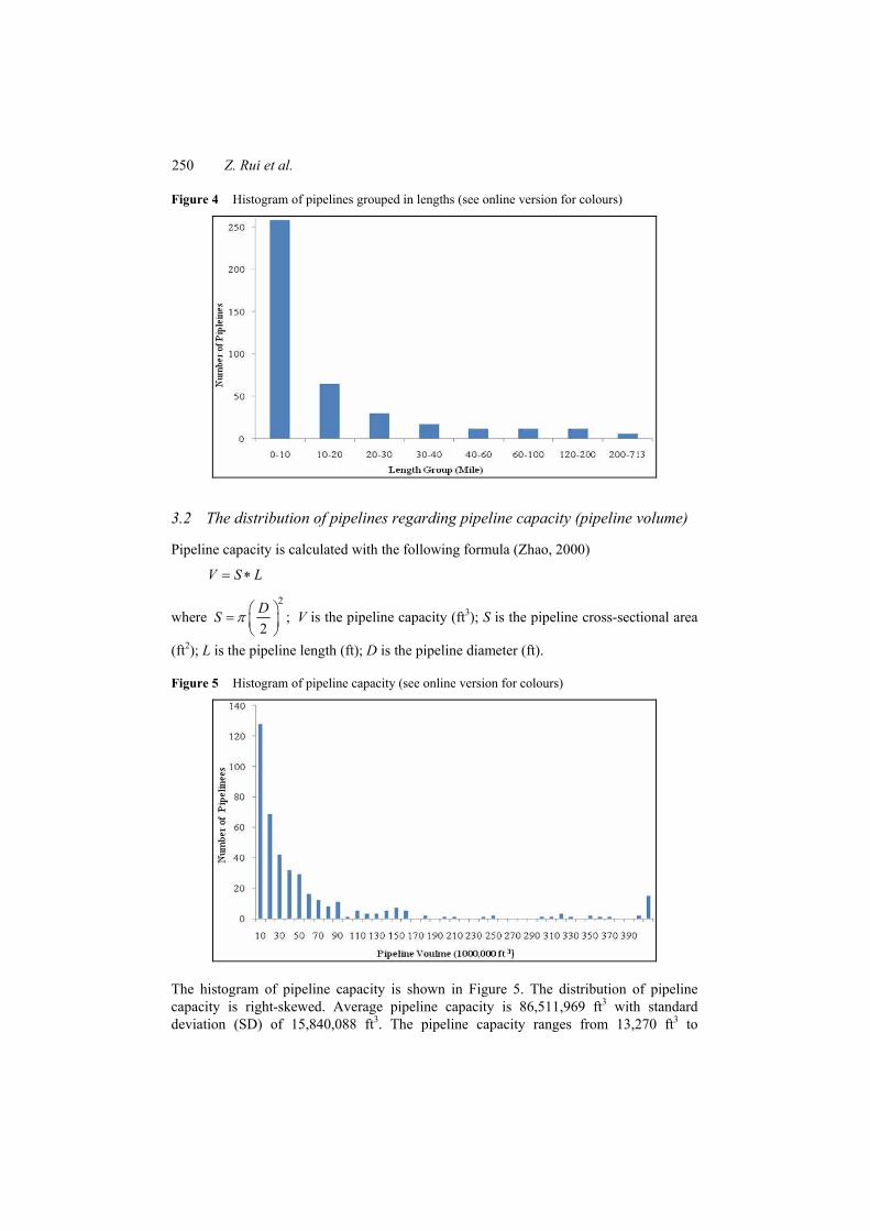
two-decades. Figure 4 displays the histogram of pipelines grouped in pipeline lengths.
The distribution of pipeline length is right-skewed. The pipeline length ranges from
Historical pipeline construction cost analysis 249
0.01 mile to 713 miles. There are 258 (62.6% of the total) pipelines in the 0 to 10 mile
group, and 65 pipelines in the 10 to 20 mile group, but only 30 (7.3% of the total) of
pipelines are longer than 60 miles. It indicates that majority of the reported pipelines are
short pipelines.
Figure 2 Histogram of pipelines between 1992 and 2008 (see online version for colours)
Figure 3 Histogram of pipelines in diameters (see online version for colours)
250 Z. Rui et al.
Figure 4 Histogram of pipelines grouped in lengths (see online version for colours)
3.2 The distribution of pipelines regarding pipeline capacity (pipeline volume)
Pipeline capacity is calculated with the following formula (Zhao, 2000)
V S L= ∗
where
2
;2
DS π ⎛ ⎞= ⎜ ⎟⎝ ⎠ V is the pipeline capacity (ft3); S is the pipeline cross-sectional area
(ft2); L is the pipeline length (ft); D is the pipeline diameter (ft).
Figure 5 Histogram of pipeline capacity (see online version for colours)
The histogram of pipeline capacity is shown in Figure 5. The distribution of pipeline
capacity is right-skewed. Average pipeline capacity is 86,511,969 ft3 with standard
deviation (SD) of 15,840,088 ft3. The pipeline capacity ranges from 13,270 ft3 to
Historical pipeline construction cost analysis 251
5,215,691,727 ft3. 58.29% of pipelines’ capacity is less than 30,000,000 ft3, and only
3.64% of pipelines’ capacity is larger than 400,000,000 ft3.
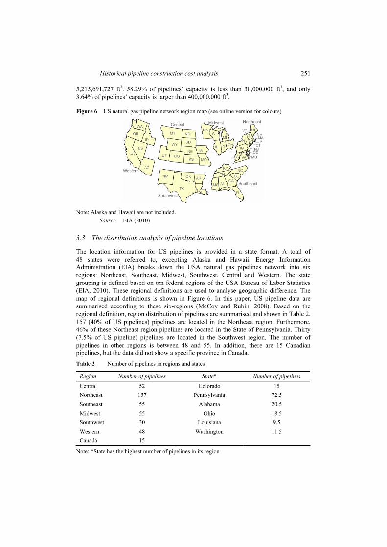
Figure 6 US natural gas pipeline network region map (see online version for colours)
Note: Alaska and Hawaii are not included.
Source: EIA (2010)
3.3 The distribution analysis of pipeline locations
The location information for US pipelines is provided in a state format. A total of
48 states were referred to, excepting Alaska and Hawaii. Energy Information
Administration (EIA) breaks down the USA natural gas pipelines network into six
regions: Northeast, Southeast, Midwest, Southwest, Central and Western. The state
grouping is defined based on ten federal regions of the USA Bureau of Labor Statistics
(EIA, 2010). These regional definitions are used to analyse geographic difference. The
map of regional definitions is shown in Figure 6. In this paper, US pipeline data are
summarised according to these six-regions (McCoy and Rubin, 2008). Based on the
regional definition, region distribution of pipelines are summarised and shown in Table 2.
157 (40% of US pipelines) pipelines are located in the Northeast region. Furthermore,
46% of these Northeast region pipelines are located in the State of Pennsylvania. Thirty
(7.5% of US pipeline) pipelines are located in the Southwest region. The number of
pipelines in other regions is between 48 and 55. In addition, there are 15 Canadian
pipelines, but the data did not show a specific province in Canada.
Table 2 Number of pipelines in regions and states
Region Number of pipelines State* Number of pipelines
Central 52 Colorado 15
Northeast 157 Pennsylvania 72.5
Southeast 55 Alabama 20.5
Midwest 55 Ohio 18.5
Southwest 30 Louisiana 9.5
Western 48 Washington 11.5
Canada 15
Note: *State has the highest number of pipelines in its region.
252 Z. Rui et al.
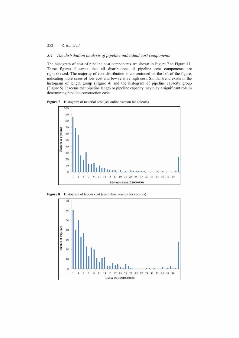
3.4 The distribution analysis of pipeline individual cost components
The histogram of cost of pipeline cost components are shown in Figure 7 to Figure 11.
These figures illustrate that all distributions of pipeline cost components are
right-skewed. The majority of cost distribution is concentrated on the left of the figure,
indicating more cases of low cost and few relative high cost. Similar trend exists in the
histogram of length group (Figure 4) and the histogram of pipeline capacity group
(Figure 5). It seems that pipeline length or pipeline capacity may play a significant role in
determining pipeline construction costs.
Figure 7 Histogram of material cost (see online version for colours)
Figure 8 Histogram of labour cost (see online version for colours)
Historical pipeline construction cost analysis 253
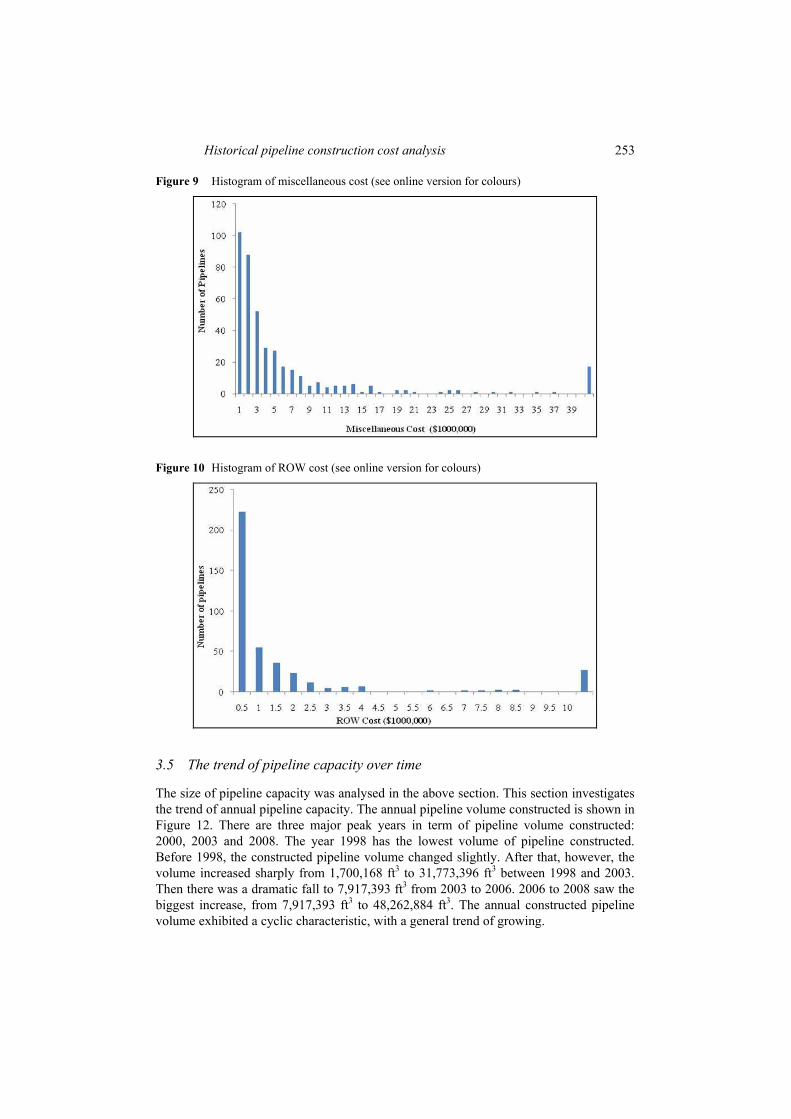
Figure 9 Histogram of miscellaneous cost (see online version for colours)
Figure 10 Histogram of ROW cost (see online version for colours)
3.5 The trend of pipeline capacity over time
The size of pipeline capacity was analysed in the above section. This section investigates
the trend of annual pipeline capacity. The annual pipeline volume constructed is shown in
Figure 12. There are three major peak years in term of pipeline volume constructed:
2000, 2003 and 2008. The year 1998 has the lowest volume of pipeline constructed.
Before 1998, the constructed pipeline volume changed slightly. After that, however, the
volume increased sharply from 1,700,168 ft3 to 31,773,396 ft3 between 1998 and 2003.
Then there was a dramatic fall to 7,917,393 ft3 from 2003 to 2006. 2006 to 2008 saw the
biggest increase, from 7,917,393 ft3 to 48,262,884 ft3. The annual constructed pipeline
volume exhibited a cyclic characteristic, with a general trend of growing.
254 Z. Rui et al.
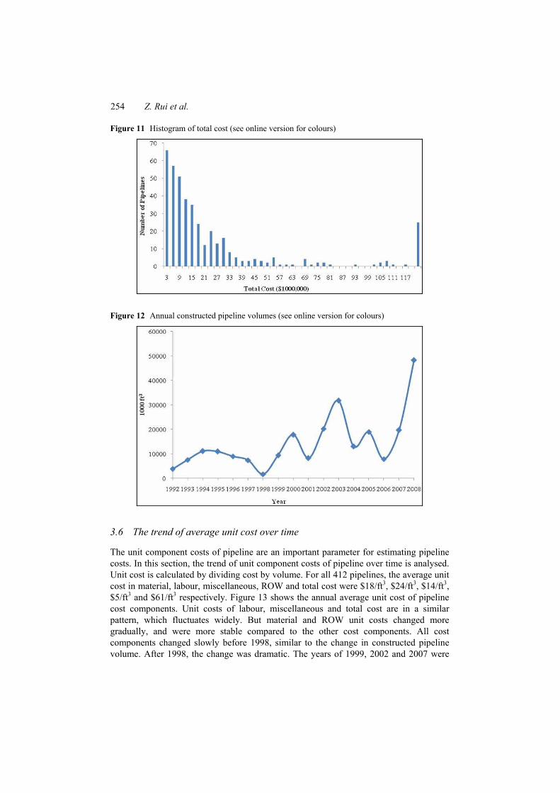
Figure 11 Histogram of total cost (see online version for colours)
Figure 12 Annual constructed pipeline volumes (see online version for colours)
3.6 The trend of average unit cost over time
The unit component costs of pipeline are an important parameter for estimating pipeline
costs. In this section, the trend of unit component costs of pipeline over time is analysed.
Unit cost is calculated by dividing cost by volume. For all 412 pipelines, the average unit
cost in material, labour, miscellaneous, ROW and total cost were $18/ft3, $24/ft3, $14/ft3,
$5/ft3 and $61/ft3 respectively. Figure 13 shows the annual average unit cost of pipeline
cost components. Unit costs of labour, miscellaneous and total cost are in a similar
pattern, which fluctuates widely. But material and ROW unit costs changed more
gradually, and were more stable compared to the other cost components. All cost
components changed slowly before 1998, similar to the change in constructed pipeline
volume. After 1998, the change was dramatic. The years of 1999, 2002 and 2007 were
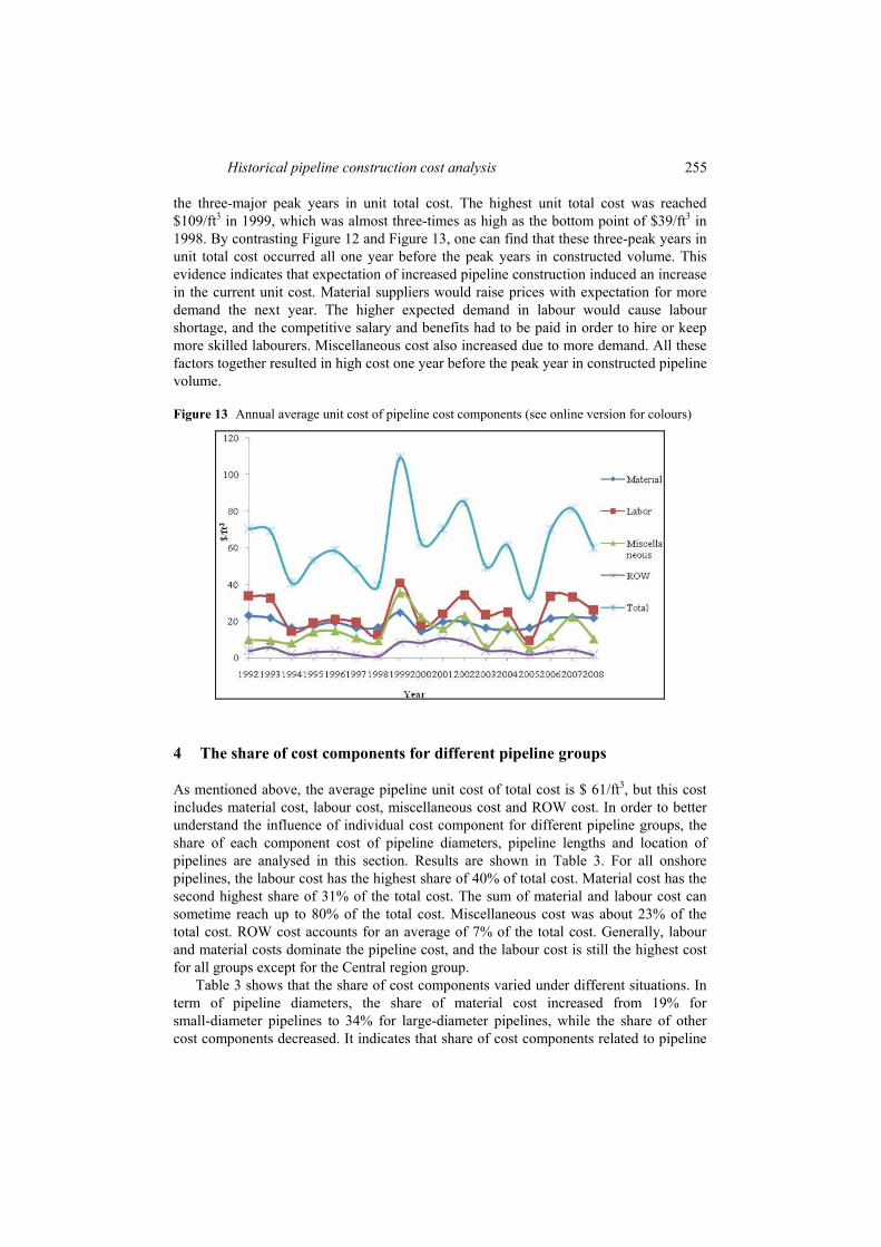
Historical pipeline construction cost analysis 255
the three-major peak years in unit total cost. The highest unit total cost was reached
$109/ft3 in 1999, which was almost three-times as high as the bottom point of $39/ft3 in
1998. By contrasting Figure 12 and Figure 13, one can find that these three-peak years in
unit total cost occurred all one year before the peak years in constructed volume. This
evidence indicates that expectation of increased pipeline construction induced an increase
in the current unit cost. Material suppliers would raise prices with expectation for more
demand the next year. The higher expected demand in labour would cause labour
shortage, and the competitive salary and benefits had to be paid in order to hire or keep
more skilled labourers. Miscellaneous cost also increased due to more demand. All these
factors together resulted in high cost one year before the peak year in constructed pipeline
volume.
Figure 13 Annual average unit cost of pipeline cost components (see online version for colours)
4 The share of cost components for different pipeline groups
As mentioned above, the average pipeline unit cost of total cost is $ 61/ft3, but this cost
includes material cost, labour cost, miscellaneous cost and ROW cost. In order to better
understand the influence of individual cost component for different pipeline groups, the
share of each component cost of pipeline diameters, pipeline lengths and location of
pipelines are analysed in this section. Results are shown in Table 3. For all onshore
pipelines, the labour cost has the highest share of 40% of total cost. Material cost has the
second highest share of 31% of the total cost. The sum of material and labour cost can
sometime reach up to 80% of the total cost. Miscellaneous cost was about 23% of the
total cost. ROW cost accounts for an average of 7% of the total cost. Generally, labour
and material costs dominate the pipeline cost, and the labour cost is still the highest cost
for all groups except for the Central region group.
Table 3 shows that the share of cost components varied under different situations. In
term of pipeline diameters, the share of material cost increased from 19% for
small-diameter pipelines to 34% for large-diameter pipelines, while the share of other
cost components decreased. It indicates that share of cost components related to pipeline
256 Z. Rui et al.
size, which agrees with Zhao’s (2000) finding. It also indicates that the share of material
cost increased when pipeline diameter increased. In term of pipeline lengths, the share of
material cost rose from 28% for short pipelines to 35% for long pipelines, with share of
the other cost components decreasing except ROW, which was constant at 7% regardless
of the total pipeline length. Therefore, the share of material cost increased when pipeline
diameter and length increased, but the labour cost maintained as the no. 1 cost component
for all diameters and lengths, averaging 40% of total cost. Furthermore, the shares of cost
components were different for different regions. The material cost in the Central region
made up around 41% of the total cost, while it was only 24% of the total cost in the
Northeast and Southeast regions. The share of labour cost is between 34% and 48% in
different regions. Miscellaneous cost was often a small part of the total cost, but the share
of miscellaneous cost in the Southeast region reached to 30% of the total cost, even
higher than share of material cost. The share of ROW cost of US pipelines ranged from
4% to 12% of total cost, while the share of ROW cost in Canada share was only 1% of
total cost. The lower share of ROW cost for Canada pipelines allows us to conclude that
Canada has less ROW issues than the US does. The share of material cost and labour cost
were approximately the same for Canadian pipelines, about 40%. The results agree with
the conclusion that the shares of labour and material costs varied by countries (Zhao,
2000). It also support that the shares of cost components vary in different regions of US
local regions or countries with no pipeline producing capacity may have high material
cost, and the pipeline cost can be reduced by developing technology to produce pipeline
materials (Zhao, 2000). The high share of labour cost was possibly caused by local high
cost of living. For example, the Northeast region had the highest labour cost compared to
the other regions. Hence, studies on share of cost components will provide useful
information for pipeline companies to estimate pipeline cost and reduce the total cost by
some actions, such as improving pipeline production capacity.
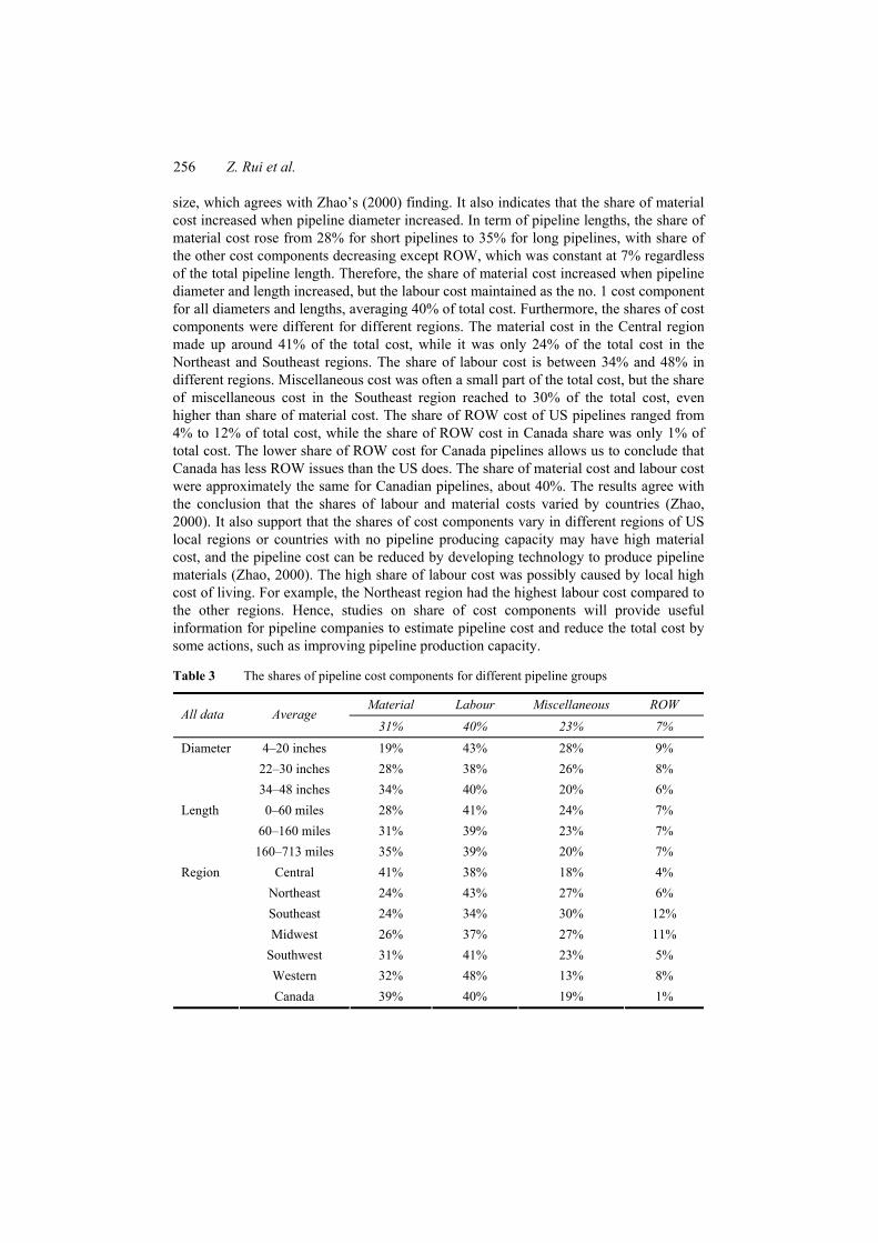
Table 3 The shares of pipeline cost components for different pipeline groups
Material Labour Miscellaneous ROW All data Average
31% 40% 23% 7%
4–20 inches 19% 43% 28% 9%
22–30 inches 28% 38% 26% 8%
Diameter
34–48 inches 34% 40% 20% 6%
0–60 miles 28% 41% 24% 7%
60–160 miles 31% 39% 23% 7%
Length
160–713 miles 35% 39% 20% 7%
Central 41% 38% 18% 4%
Northeast 24% 43% 27% 6%
Southeast 24% 34% 30% 12%
Midwest 26% 37% 27% 11%
Southwest 31% 41% 23% 5%
Western 32% 48% 13% 8%
Region
Canada 39% 40% 19% 1%
Historical pipeline construction cost analysis 257
5 Learning curve (learning-by-doing) in pipeline construction
5.1 Introduction to learning curve
The productivity of technology and labour normally increases as workers engage in
repetitive tasks. The unit costs typically decline with cumulative production. The learning
curve is derived from historical observation to measure learning by doing, and it is
helpful for cost estimators and analysts. The learning curve theory is based on these
assumptions:
1 the unit cost required to perform a task decreases as the task is repeated
2 the unit cost reduces at a decreasing rate
3 the rate of improvement has sufficient consistency to allow its use as a prediction
tool (Federal Aviation Administration, 2005).
The consistence in improvement is expressed as the percentage reduction in cost with
doubled quantities of product. The constant percentage is called the learning rate. For
example, a 20% learning rate implies the cost is reduced to 80% of its previous level after
a doubling of cumulative capacity.
The learning curve is normally exhibited in power function form and linear function
form. The power function form is shown below (Federal Aviation Administration, 2005):
1b
xY T X= i
where Yx is the average cost of the first X units; T1 is the theoretical cost of the first
production unit; X is the sequential number of the last unit in the quantity for which the
average to be computed; b is a constant reflecting the rate costs decrease from unit to
unit; 2b and 1–2b are called progress ratio and learning rate respectively (Federal Aviation
Administration, 2005; International Energy Agency, 2000).
Learning curve function is normally expressed in log-log paper as a string line.
Straight lines are more easily for analysts to extend beyond the range of data (Federal
Aviation Administration, 2005). Take the logarithms of the both sides to get a straight
line equation,
Y bX C= +
where ( )log , log , log 1 .xY Y X X C T↓= = =
The learning curve effect is a complicated process. Some of major reasons for
learning-by-doing effect are: intensive use of skilled labour, a high degree of capital,
research and development intensity, fast market growth and interaction between supply
and demand (Wilkinson, 2005). In addition, accumulated learning has a start-up and a
steady period. The cost reduction is significant in the start-up period and modest in the
steady period (Grubler, 1998). It is the same for technology development. There are
significant cost improvements during R&D phase followed by more modest improvement
after commercialisation. The longer technology has been in operation, the smaller the
cost decreases (Zhao, 2000). It is possible that no further improvement in cost reduction
occurs for existing and mature technology (Grubler, 1998). The commercialisation of
technology in the oil and gas market is costly and time intensive with an average 16 years
from concepts to widespread commercial adoption (National Petroleum Council, 2007).
258 Z. Rui et al.
The range of progress ratio for technology is between 65% and 95%, and between 70%
and 90% for energy technology (Christiansson, 1995).
5.2 Selecting pipeline cost data for calculating learning rate
The cost data for learning curve analysis has to be recurring cost, because non-recurring
costs will not experience the learning effect (Federal Aviation Administration, 2005).
Zhao (2000) calculated the learning curve of the total cost without considering this
requirement and her results may be less accurate. The miscellaneous and ROW costs as
well as the total cost are not qualified for the learning curve analysis due to inclusion of
non-recurring costs. The learning curve analysis is, therefore, only conducted for material
and labour costs. The pipeline data provide the cost data from 1992 to 2008. However,
the 1999 data are considered an outlier due to extremely high cost. Hence, the 1999 data
is not used for learning curve analysis. The learning curve of the material and labour cost
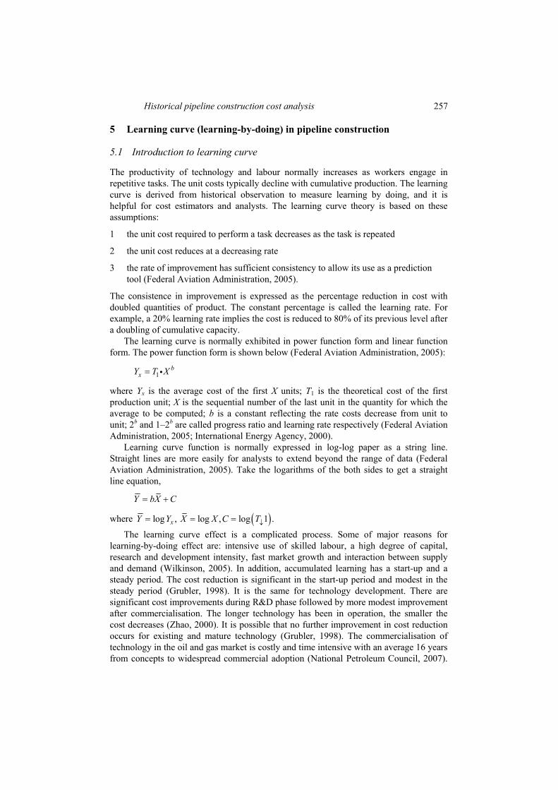
of pipelines constructed from 1992 to 2008 is presented in Figure 14. Figure 14 shows
that there was an attractive cost reduction in unit cost before 100 million ft3. After
100 million ft3, the unit cost did not show cost reduction even increases. It indicates there
was not cost reduction after 100 million ft3, which was considered as a more mature
period. In the standard experience curve theory, it is assume that learning rates do not
change over time, but the technology or labour learning are going to a more mature
phase. However, the learning curve analysis does not always strictly agree with this
assumption (Schaeffer and de Moor, 2004). In order to better fit the learning curve, the
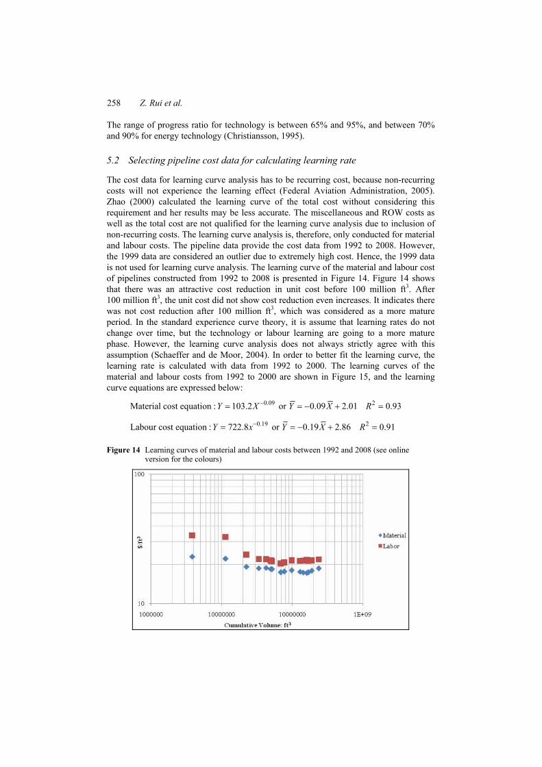
learning rate is calculated with data from 1992 to 2000. The learning curves of the
material and labour costs from 1992 to 2000 are shown in Figure 15, and the learning
curve equations are expressed below:
0.09 2Material cost equation : 103.2 or 0.09 2.01 0.93Y X Y X R−= = − + =
0.19 2Labour cost equation : 722.8 or 0.19 2.86 0.91Y x Y X R−= = − + =
Figure 14 Learning curves of material and labour costs between 1992 and 2008 (see online version for the colours)
Historical pipeline construction cost analysis 259
Figure 15 Learning curves of material and labour costs between 1992 and 2000 (see online version for colours)
Both R2 (coefficient of determination) are higher than 0.9, which indicates a very good
fit. The learning rates of labour and material cost are 12.4% and 6.1%, respectively. That
is, doubling the construction of pipeline volume, the labour cost and material cost will be
reduced by 12.4% and 6.1% respectively. But it can be noted that the cost reduction
becomes smaller with increasing volume, same as the finding of Zhao (2000).
5.3 Learning rate for different pipeline groups
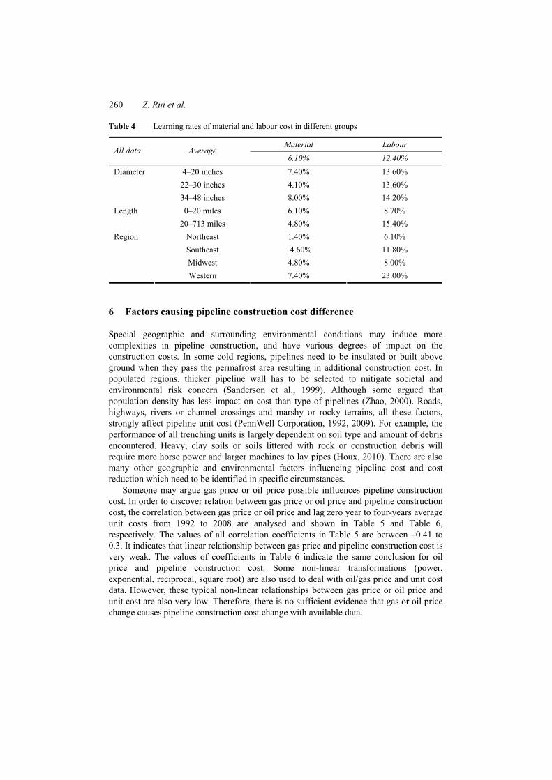
The learning rates for different pipeline diameters, lengths and locations are calculated
and shown in Table 4. In general, the learning rate of material cost was lower than the
learning rate of labour cost in all subgroups except in the Southeast region. For all
subgroups, the range of the learning rate of material cost was between 1.40% and
14.60%, and the range of the learning rate of labour cost was between 6.10% and
23.00%. For different diameters, learning rates of labour cost is between 13.60% and
14.20%, but learning rates of material cost ranges from 4.10% to 8.00%. For different
pipeline lengths, the learning rate of labour cost showed a significant difference about
6.70%. As expected, the results indicate that longer pipelines can achieve a higher
learning rate in labour cost. However, the results also show that longer pipelines have a
disadvantage on learning rate of material cost, 6.10% for zero to 20 miles pipeline and
4.80% for 20 to 713 miles pipelines. In terms of regions, the results show that the
learning rate varied widely in different regions. The Northeast region had the lowest
learning rate of material and labour cost. A plausible explanation for this finding would
be that a large amount of pipeline built in the Northeast region makes Northeast region
reach a more mature stage earlier and faster than other regions. Pipelines in the Southeast
and Western region showed higher learning rate of material and labour costs than other
regions. In summary, the above analysis reveal that learning rates varied by different
pipeline diameters, pipeline lengths and the location of pipelines at different degree.
260 Z. Rui et al.
Table 4 Learning rates of material and labour cost in different groups
Material Labour All data Average
6.10% 12.40%
4–20 inches 7.40% 13.60%
22–30 inches 4.10% 13.60%
Diameter
34–48 inches 8.00% 14.20%
0–20 miles 6.10% 8.70% Length
20–713 miles 4.80% 15.40%
Northeast 1.40% 6.10%
Southeast 14.60% 11.80%
Midwest 4.80% 8.00%
Region
Western 7.40% 23.00%
6 Factors causing pipeline construction cost difference
Special geographic and surrounding environmental conditions may induce more
complexities in pipeline construction, and have various degrees of impact on the
construction costs. In some cold regions, pipelines need to be insulated or built above
ground when they pass the permafrost area resulting in additional construction cost. In
populated regions, thicker pipeline wall has to be selected to mitigate societal and
environmental risk concern (Sanderson et al., 1999). Although some argued that
population density has less impact on cost than type of pipelines (Zhao, 2000). Roads,
highways, rivers or channel crossings and marshy or rocky terrains, all these factors,
strongly affect pipeline unit cost (PennWell Corporation, 1992, 2009). For example, the
performance of all trenching units is largely dependent on soil type and amount of debris
encountered. Heavy, clay soils or soils littered with rock or construction debris will
require more horse power and larger machines to lay pipes (Houx, 2010). There are also
many other geographic and environmental factors influencing pipeline cost and cost
reduction which need to be identified in specific circumstances.
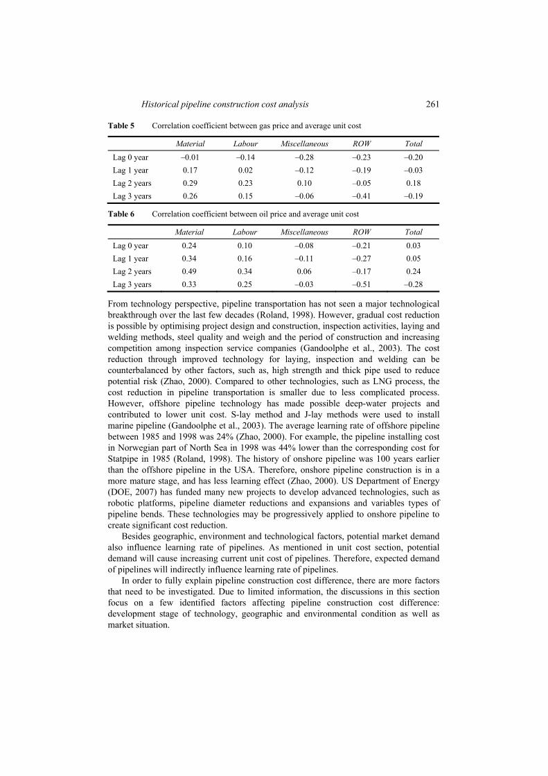
Someone may argue gas price or oil price possible influences pipeline construction
cost. In order to discover relation between gas price or oil price and pipeline construction
cost, the correlation between gas price or oil price and lag zero year to four-years average
unit costs from 1992 to 2008 are analysed and shown in Table 5 and Table 6,
respectively. The values of all correlation coefficients in Table 5 are between –0.41 to
0.3. It indicates that linear relationship between gas price and pipeline construction cost is
very weak. The values of coefficients in Table 6 indicate the same conclusion for oil
price and pipeline construction cost. Some non-linear transformations (power,
exponential, reciprocal, square root) are also used to deal with oil/gas price and unit cost
data. However, these typical non-linear relationships between gas price or oil price and
unit cost are also very low. Therefore, there is no sufficient evidence that gas or oil price
change causes pipeline construction cost change with available data.
Historical pipeline construction cost analysis 261
Table 5 Correlation coefficient between gas price and average unit cost
Material Labour Miscellaneous ROW Total
Lag 0 year –0.01 –0.14 –0.28 –0.23 –0.20
Lag 1 year 0.17 0.02 –0.12 –0.19 –0.03
Lag 2 years 0.29 0.23 0.10 –0.05 0.18
Lag 3 years 0.26 0.15 –0.06 –0.41 –0.19
Table 6 Correlation coefficient between oil price and average unit cost
Material Labour Miscellaneous ROW Total
Lag 0 year 0.24 0.10 –0.08 –0.21 0.03
Lag 1 year 0.34 0.16 –0.11 –0.27 0.05
Lag 2 years 0.49 0.34 0.06 –0.17 0.24
Lag 3 years 0.33 0.25 –0.03 –0.51 –0.28
From technology perspective, pipeline transportation has not seen a major technological
breakthrough over the last few decades (Roland, 1998). However, gradual cost reduction
is possible by optimising project design and construction, inspection activities, laying and
welding methods, steel quality and weigh and the period of construction and increasing
competition among inspection service companies (Gandoolphe et al., 2003). The cost
reduction through improved technology for laying, inspection and welding can be
counterbalanced by other factors, such as, high strength and thick pipe used to reduce
potential risk (Zhao, 2000). Compared to other technologies, such as LNG process, the
cost reduction in pipeline transportation is smaller due to less complicated process.
However, offshore pipeline technology has made possible deep-water projects and
contributed to lower unit cost. S-lay method and J-lay methods were used to install
marine pipeline (Gandoolphe et al., 2003). The average learning rate of offshore pipeline
between 1985 and 1998 was 24% (Zhao, 2000). For example, the pipeline installing cost
in Norwegian part of North Sea in 1998 was 44% lower than the corresponding cost for
Statpipe in 1985 (Roland, 1998). The history of onshore pipeline was 100 years earlier
than the offshore pipeline in the USA. Therefore, onshore pipeline construction is in a
more mature stage, and has less learning effect (Zhao, 2000). US Department of Energy
(DOE, 2007) has funded many new projects to develop advanced technologies, such as
robotic platforms, pipeline diameter reductions and expansions and variables types of
pipeline bends. These technologies may be progressively applied to onshore pipeline to
create significant cost reduction.
Besides geographic, environment and technological factors, potential market demand
also influence learning rate of pipelines. As mentioned in unit cost section, potential
demand will cause increasing current unit cost of pipelines. Therefore, expected demand
of pipelines will indirectly influence learning rate of pipelines.
In order to fully explain pipeline construction cost difference, there are more factors
that need to be investigated. Due to limited information, the discussions in this section
focus on a few identified factors affecting pipeline construction cost difference:
development stage of technology, geographic and environmental condition as well as
market situation.
262 Z. Rui et al.
7 Concluding summary
Based on historical data collected from Oil and Gas Journal, the distribution of pipelines
in term of year of completion, pipeline diameters, pipeline lengths, pipeline capacity and
location of pipelines are analysed. Among the data examined, 78.3% of pipelines were
less than 20 miles, 52.9% of them had a diameter of 30 inches or larger and 58% of
pipelines’ capacities was less than 30,000,000 ft3. The pipelines were located across the
USA, but about 40% of them were located in the Northeast region. The distributions of
cost of pipeline cost components were all right-skewed (Figure 7 to Figure 11), and the
range of cost of pipeline cost components was very large. The trend of annual constructed
pipeline volume and annual average unit cost indicates that expecting of increased
pipeline demand will causes increasing currently unit cost. Shares of cost components are
different for various pipeline diameters, pipeline lengths and locations of pipelines. The
material and labour cost are major component of pipeline construction (Table 3). Results
of learning curve analysis show that learning rate also varied by pipeline diameters,
pipeline lengths, locations of pipelines (Table 4). Furthermore, development stage of
pipeline technology, site characteristics and market condition are identified as the factors
influencing pipeline construction cost difference.
References
Central Intelligence Agency (2008) The World Factbook, available at https://www.cia.gov/library/publications/the-world-factbook (accessed on 9 January 2010).
Chemical Engineering (2009) Chemical Engineering’s Plant Cost Index, available at http://www.che.com/pci (accessed on 4 January 2010).
Christiansson, L. (1995) ‘Diffusion and learning curves of renewable energy technologies’, pp.95–126, Working paper, International Institute for Applied System Analysis, Austria.
DOE (2007) ‘Transmission, distribution and storage’, available at http://www.fe.doe.gov/programs/oilgas/delivery/index.html (accessed on 3 January 2007).
Energy Information Administration (EIA) (2010) ‘Natural gas transportation maps’, available at http://www.eia.doe.go (accessed on 9 January 2010).
Federal Aviation Administration (2005) FAA Pricing Handbook, available at http://www.fast.faa.gov/pricing/index.htm (accessed on 9 January 2010).
Gandoolphe, S.C., Appert, O. and Dickel, R. (2003) ‘The challenges of future cost reductions for new supply options (pipeline, LNG, GTL)’, Paper Presented at the 22nd World Gas Conference, 1–5 June, Tokyo, Japan.
Grubler, A. (1998) Technology and Global Change, Cambridge University Press.
Heddle, G., Herzog, H. and Klett, M. (2003) The Economics of CO2 Storage, MIT LFEE 2003-003 RP, Laboratory for Energy and Environment, Massachusetts Institute of Technology.
Houx, J. (2010) ‘Trench warfare’, Grounds Maintenance, available at http://www.grounds-mag.com/mag/grounds_maintenance_trench_warfare (accessed on 9 January 2010).
International Energy Agency (2000) Experience Curves for Energy Technology Policy, Paris, France.
McCoy, S.T. and Rubin, E.S. (2008) ‘An engineering-economic model of pipeline transport of CO2 with application to carbon capture and storage’, International Journal of Greenhouse Gas Control, Vol. 2, No. 2, pp.219–229.
Historical pipeline construction cost analysis 263
National Petroleum Council (2007) ‘Oil and gas technology development’, available at http://www.npc.org (accessed on 9 January 2010).
Parker, N.C. (2004) Using Natural Gas Transmission Pipeline Costs to Estimate Hydrogen Pipeline Costs, Research Report UCD-ITS-RR-04-35, Institute of Transportation Studies, University of California, Davis.
PennWell Corporation (1992, 2009) Oil & Gas Journal Databook, Tulsa, Oklahoma.
Roland, K. (1998) ‘Technology will continue to profoundly affect energy industry’, Oil & Gas Journal, Vol. 96, No. 13, pp.69–74.
Sanderson, N., Ohm, R. and Jacobs, M. (1999) ‘Study of X-100 line pipe costs points to potential savings’, Oil & Gas Journal, Vol. 11, pp.54–56.
Schaeffer, G.J. and de Moor, H.H.C. (2004) ‘Learning in PV trends and future prospects’, Paper Presented at the 19th European PV Solar Energy Conference and Exhibition, 7–11 June, Paris, France.
Scheduble, K.L. (2002) ‘Trenchless technologies in pipeline construction’, Journal for Piping, Engineering, Practice, Special edition, pp.1–17.
Wilkinson, N. (2005) Managerial Economics: A Problem-Solving Approach, Cambridge University Press.
Zhang, C, Yan, D., and Zhang, Y. (2007) ‘The design procedure model study of gas transmission pipeline’, Oil & Gas Storage and Transportation, Vol. 26, No. 7, pp.18–20.
Zhao, J. (2000) ‘Diffusion, costs and learning in the development of international gas transmission lines’, Working paper IR-00-054, International Institute for Applied Systems Analysis, Austria.