Embed Size (px)
Citation preview
Understanding the In-Camera Image Processing Pipeline for
Computer Vision
IEEE CVPR 2016June 26, 2016
1
Michael S. BrownNational University of Singapore
(York University, Canada)

Tutorial schedule
• Part 1 (General Part)
– Motivation
– Review of color/color spaces
– Overview of camera imaging pipeline
• Part 2 (Specific Part)
– Modeling the in-camera color pipeline
– Photo-refinishing
• Part 3 (Wrap Up)
– The good, the bad, and the ugly of commodity cameras and computer vision research
– Concluding remarks2
8.30am-10.25am
Coffee Break10.25am – 11am
11.00am-12.30pm

Motivation for this tutorial?
3
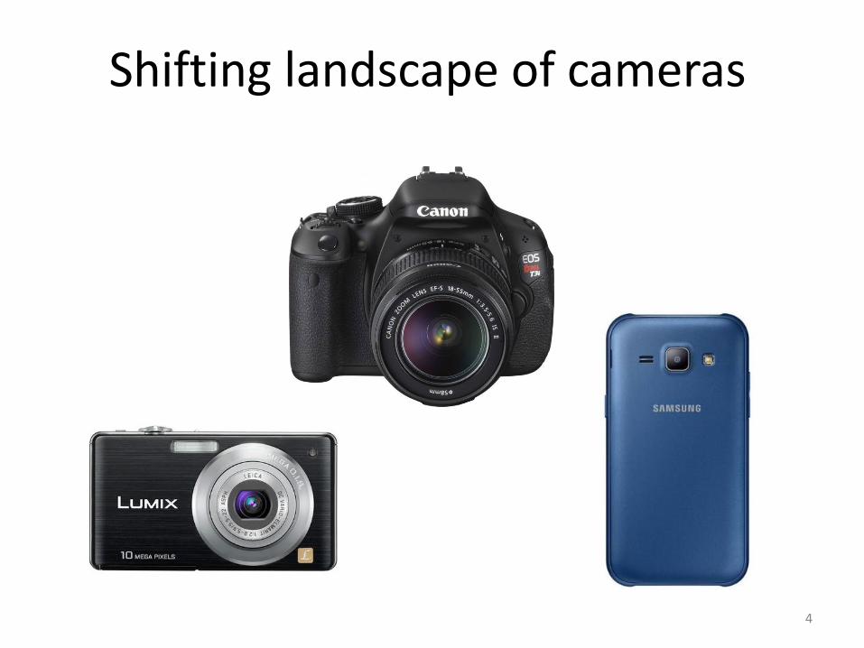
Shifting landscape of cameras
4

Market Analysis byMayflower Concepts
5
Film
Point & Shoot
DSLR/Mirrorless
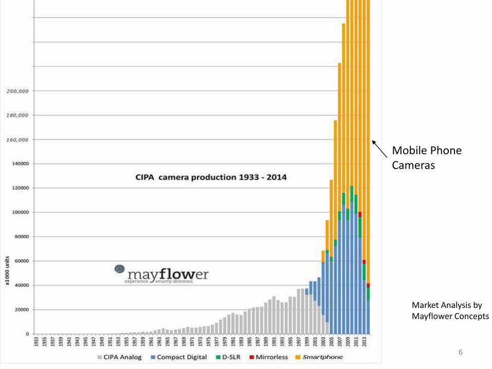
Market Analysis byMayflower Concepts
6
Mobile PhoneCameras
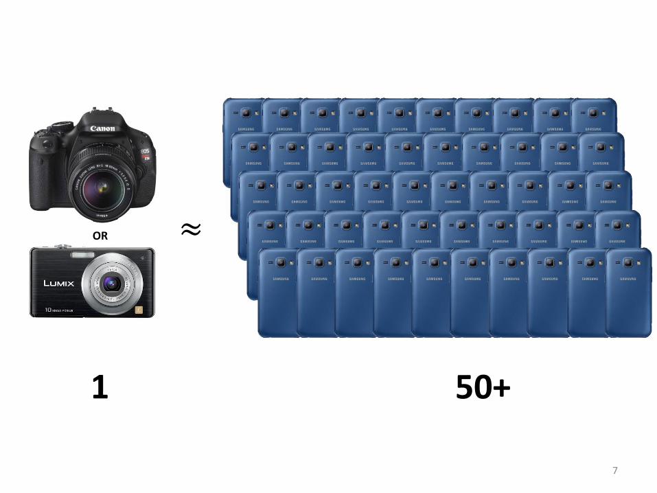
OR
1
≈
50+
7
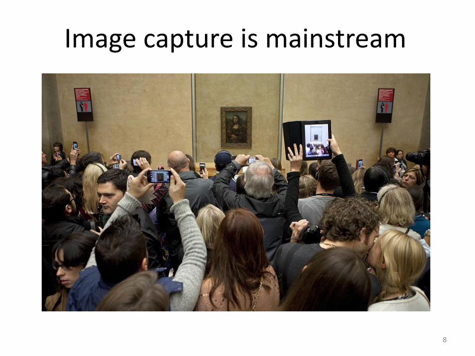
Image capture is mainstream
8
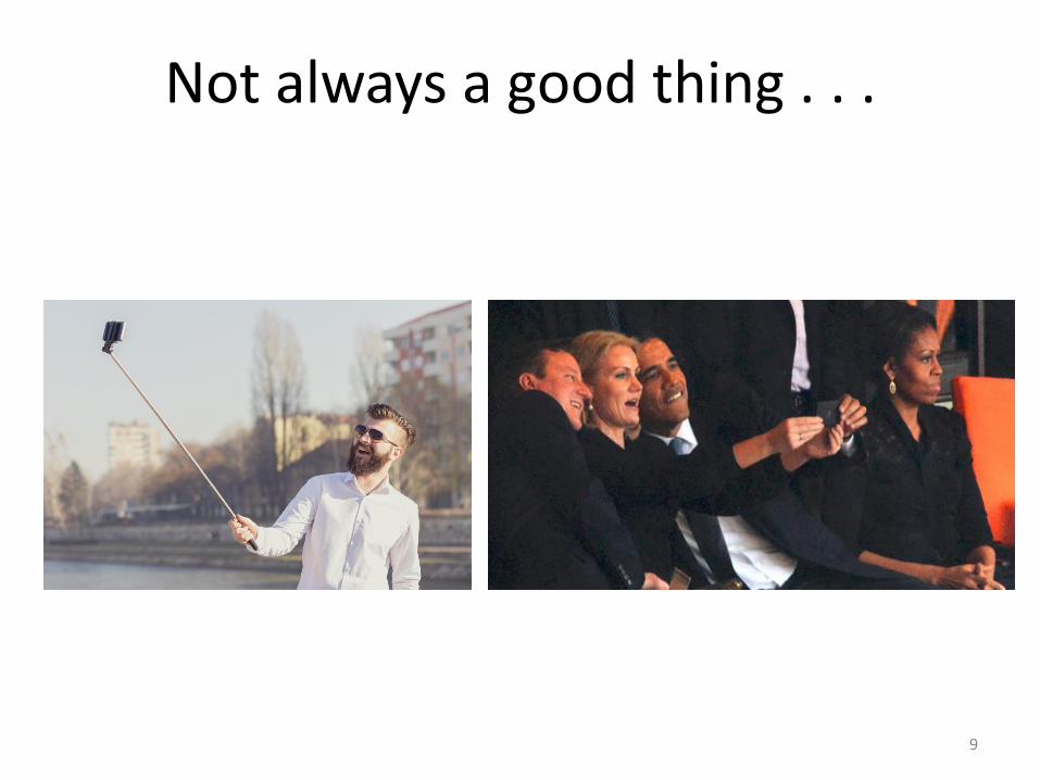
Not always a good thing . . .
9

Imaging for more than photography
Many applications are not necessarily interested in the actual
photo.
10
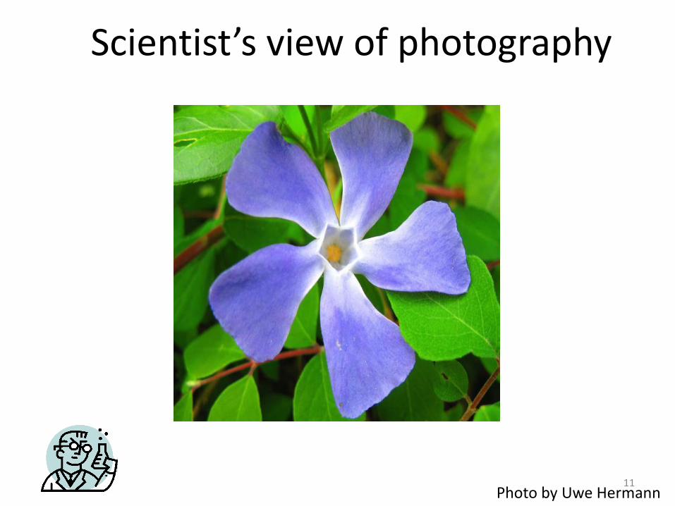
Scientist’s view of photography
Photo by Uwe Hermann11
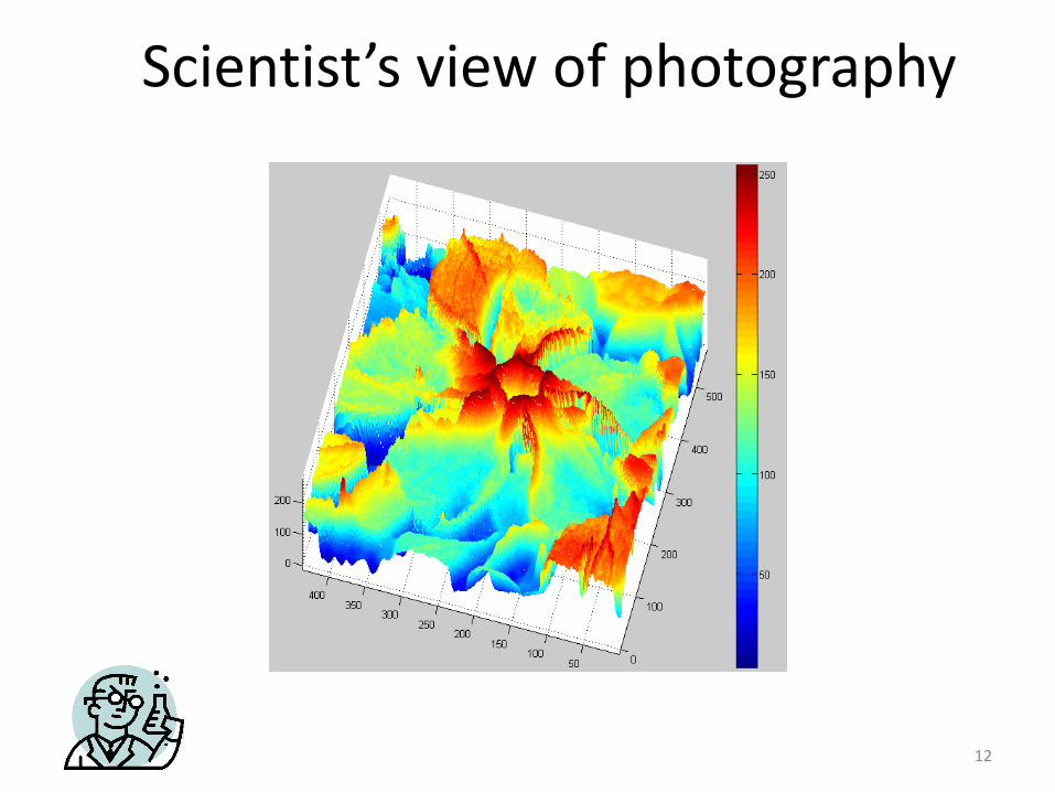
Scientist’s view of photography
12
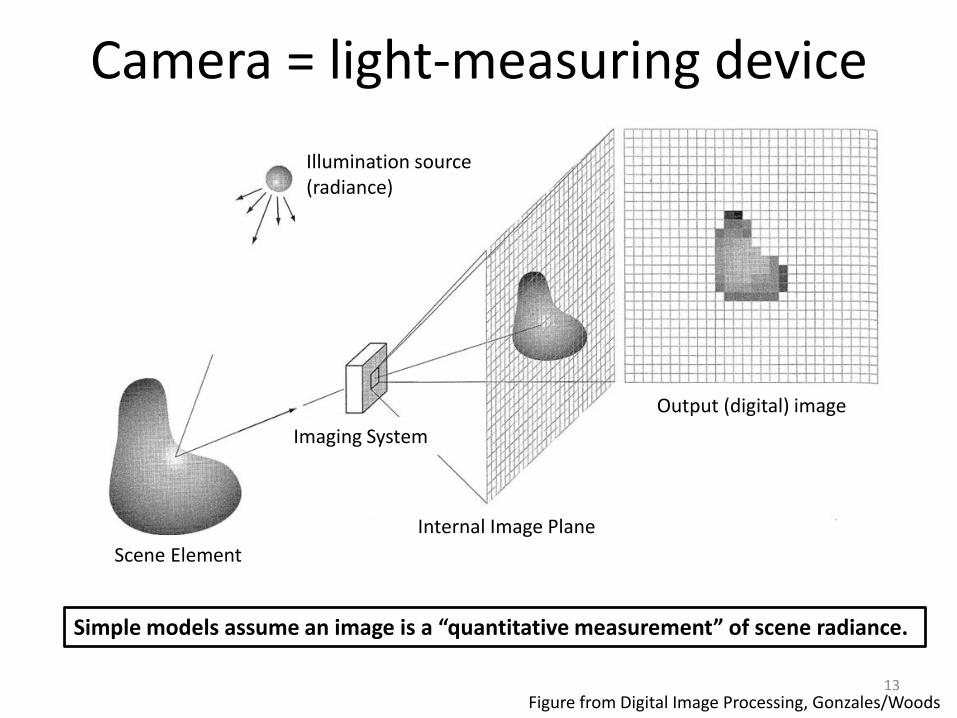
Camera = light-measuring device
Simple models assume an image is a “quantitative measurement” of scene radiance.
Illumination source(radiance)
Internal Image Plane
Scene Element
Imaging System
Output (digital) image
Figure from Digital Image Processing, Gonzales/Woods13
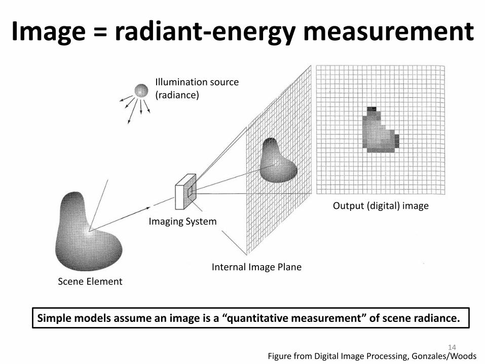
Image = radiant-energy measurement
Simple models assume an image is a “quantitative measurement” of scene radiance.
Illumination source(radiance)
Internal Image Plane
Scene Element
Imaging System
Output (digital) image
Figure from Digital Image Processing, Gonzales/Woods14

Assumption used in many places
• Shape from shading• HDR Imaging• Image Matching• Color constancy• Etc . . .
Shape-from-shading
Image matching
From Lu et al, CVPR’10
From Jon Mooser, CGIT Lab, USC From O’Reilly’s digital media forum
HDR imaging
15
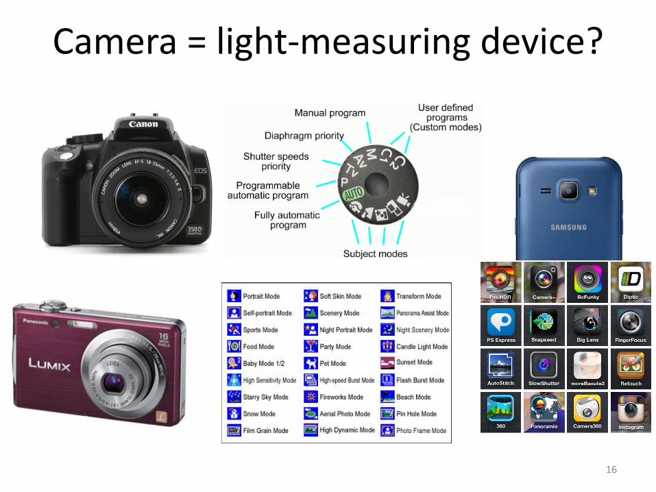
Camera = light-measuring device?
16
Samsung Galaxy S6 edge HTC One M9
LG G4
Google Camera AppAll settings the same
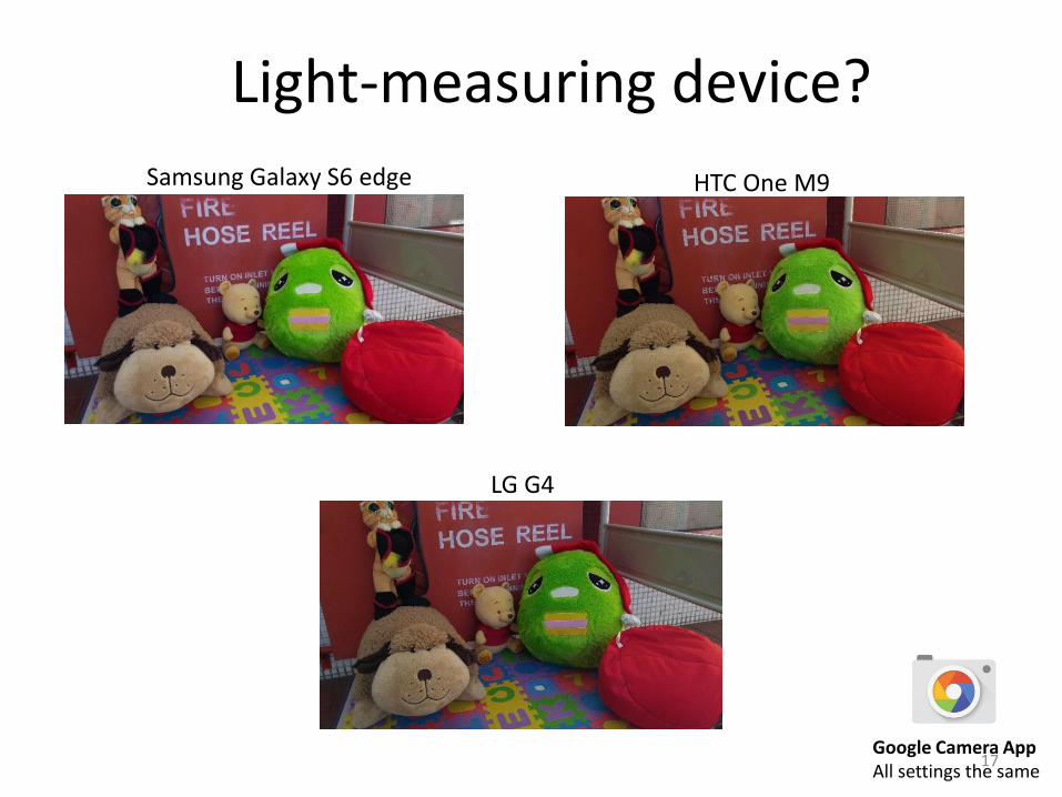
Light-measuring device?
17

Onboard processing (photo finishing)“Secret recipe” of a camera
Photographs taken from three different cameras with the same aperture, shutter speed, white-balance , ISO, and picture style.
18
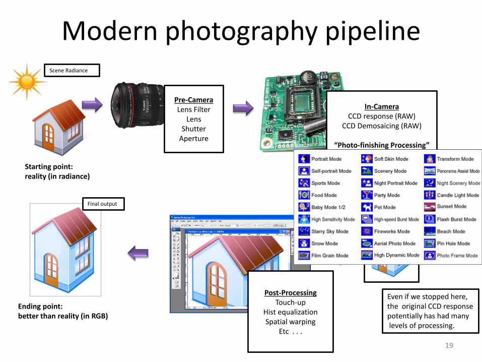
Modern photography pipeline
In-CameraCCD response (RAW)
CCD Demosaicing (RAW)
“Photo-finishing Processing”
Scene Radiance
Pre-CameraLens Filter
LensShutter
Aperture
Post-ProcessingTouch-up
Hist equalizationSpatial warping
Etc . . .
Starting point: reality (in radiance)
Final output
Ending point: better than reality (in RGB)
Camera Output: sRGB
Even if we stopped here,the original CCD responsepotentially has had manylevels of processing.
19
Digital cameras
• Digital cameras are far from being light-measuring devices
• They are designed to produce visually pleasing photographs
• There is a great deal of processing (photo-finishing) happening on the camera
The goal of this tutorial is to discuss common processing steps that take place
onboard consumer cameras
20
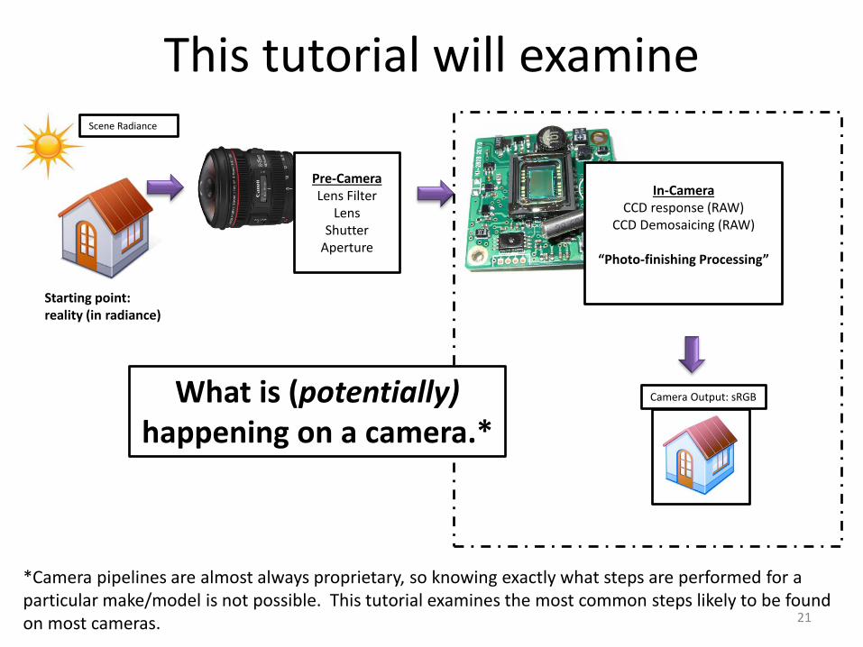
This tutorial will examine
In-CameraCCD response (RAW)
CCD Demosaicing (RAW)
“Photo-finishing Processing”
Scene Radiance
Pre-CameraLens Filter
LensShutter
Aperture
Starting point: reality (in radiance)
Camera Output: sRGBWhat is (potentially) happening on a camera.*
*Camera pipelines are almost always proprietary, so knowing exactly what steps are performed for a particular make/model is not possible. This tutorial examines the most common steps likely to be found on most cameras. 21

Tutorial schedule
• Part 1 (General Part)
– Motivation
– Review of color/color spaces
– Overview of camera imaging pipeline
• Part 2* (Specific Part)
– Modeling the in-camera color pipeline
– Photo-refinishing
• Part 3 (Wrap Up)
– The good, the bad, and the ugly of commodity cameras and computer vision research
– Concluding Remarks
22* Mainly involves shameless self-promotion of my group’s work.

“Crash Course” on Color & Color Spaces
23

Color
Def Color (noun): The property possessed by an object of producing different sensations on the eye as a result of the way it reflects or emits light.
Oxford Dictionary
Def Colour (noun): The word color spelt with the letter ‘u’ and pronounced with a non-American accent.
24
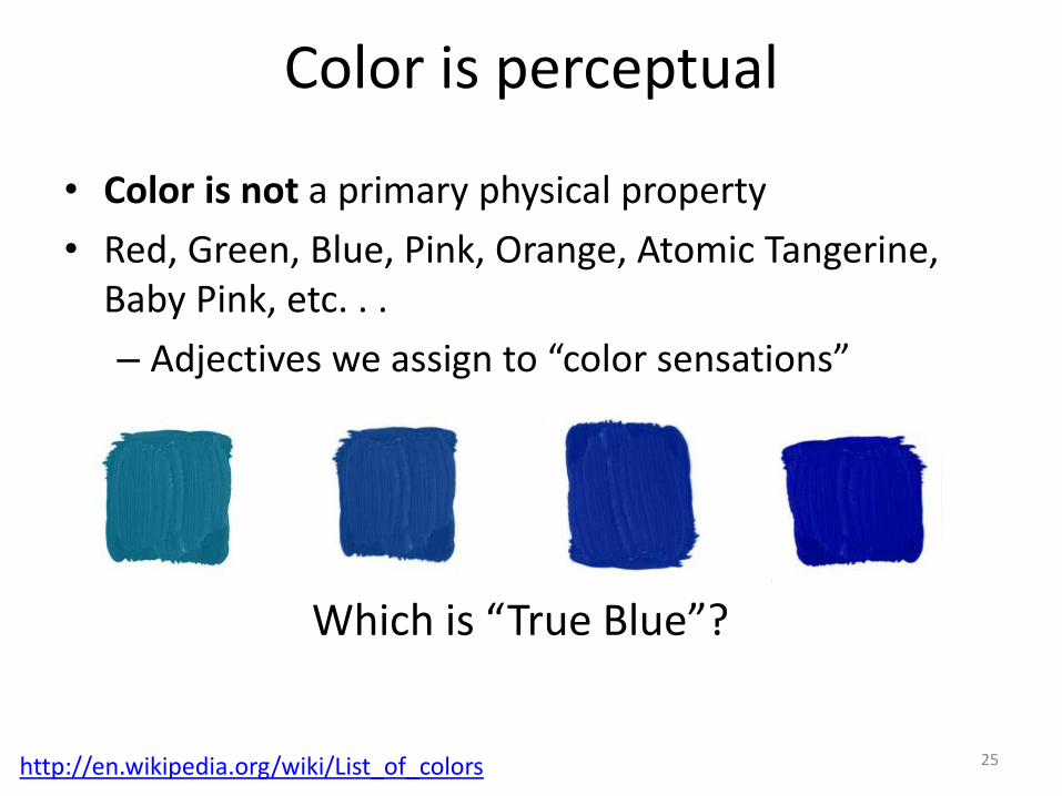
Color is perceptual
• Color is not a primary physical property
• Red, Green, Blue, Pink, Orange, Atomic Tangerine, Baby Pink, etc. . .
– Adjectives we assign to “color sensations”
http://en.wikipedia.org/wiki/List_of_colors
Which is “True Blue”?
25

Subjective terms to describe color
Hue Name of the color(yellow, red, blue, green, . . . )
Value/Lightness/BrightnessHow light or dark a color is.
Saturation/Chroma/Color Purity How “strong” or “pure” a color is.
Image from Benjamin SalleyA page from a Munsell Student Color Set
Hue
Chroma
Val
ue
26
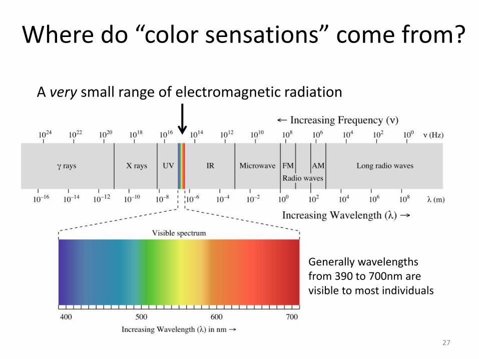
Where do “color sensations” come from?
A very small range of electromagnetic radiation
Generally wavelengthsfrom 390 to 700nm arevisible to most individuals
27
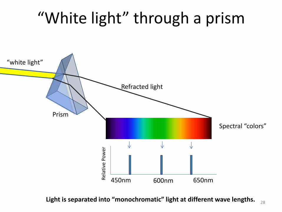
“White light” through a prism
Light is separated into “monochromatic” light at different wave lengths.
450nm 600nm 650nm
“white light”
Refracted light
Rel
ativ
e Po
wer
Prism
Spectral “colors”
28
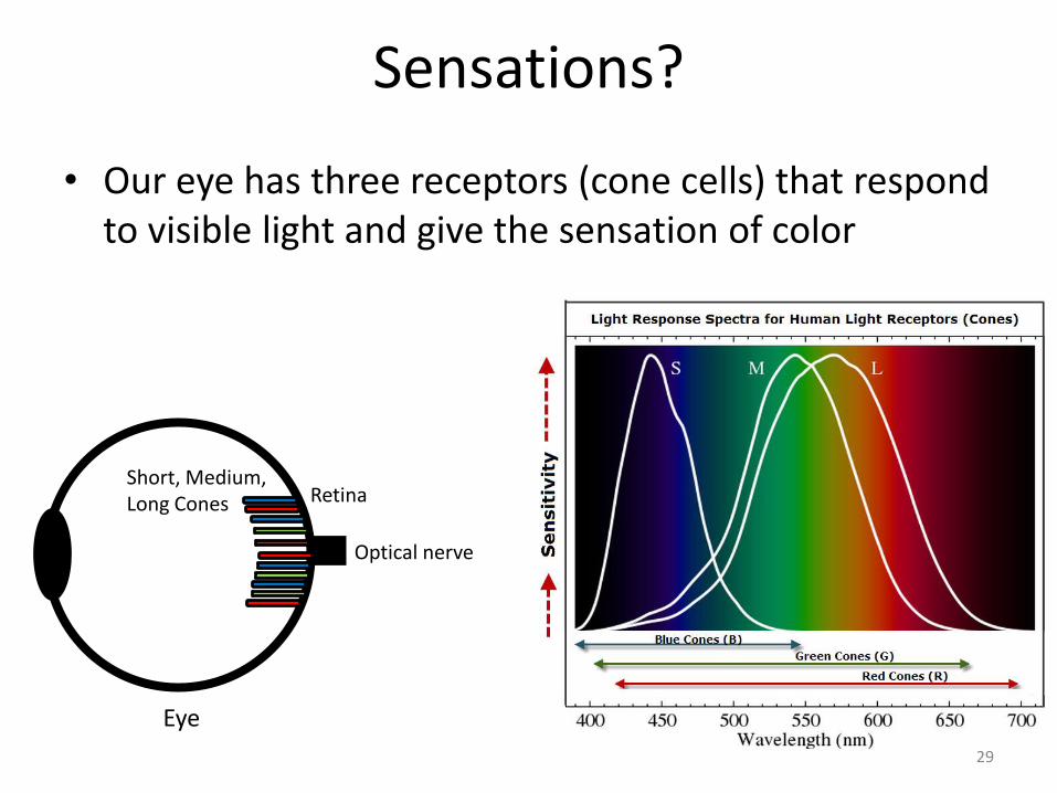
Sensations?
• Our eye has three receptors (cone cells) that respond to visible light and give the sensation of color
Eye
Short, Medium,Long Cones Retina
Optical nerve
29
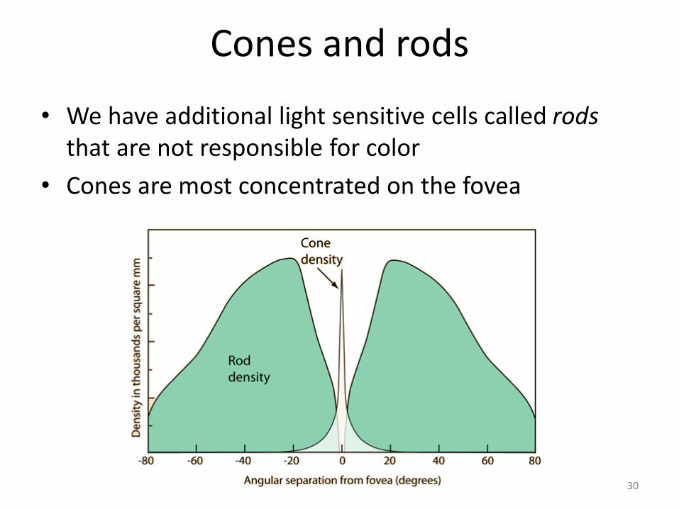
Cones and rods
• We have additional light sensitive cells called rodsthat are not responsible for color
• Cones are most concentrated on the fovea
30

Spectral power distribution (SPD)
We rarely see monochromatic light in real world scenes. Instead, objects reflect a wide range of wavelengths. This can be described by a spectral power distribution (SPD) shown above. The SPD plot shows the relative amount of each wavelength reflected over the visible spectrum. 31

SPD relation to color is not unique
• Due to the accumulation effect of the cones, two different SPDs can be perceived as the same color
Lettuce SPD
stimulating
S=0.2, M=0.8,
L=0.8
Green ink SPD
stimulating
S=0.2, M=0.8,
L=0.8
Lettuce SPD
Green Ink SPD
SPD of “real lettuce”
SPD of ink in a “picture of lettuce”
Result in the samecolor “sensation”.
32
Tristimulus color theory
• Even before cone cells were discovered, it was empirically found that only three distinct colors (primaries) could be mixed to produce other colors
• Thomas Young (1803), Hermann von Helmholtz (1852), Hermann Grassman (1853), James Maxwell (1856) all explored the theory of trichromacy for human vision
33
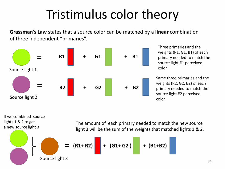
Tristimulus color theoryGrassman’s Law states that a source color can be matched by a linear combination of three independent “primaries”.
=
=
R1 + G1 + B1
R2 + G2 + B2
Source light 1
Source light 2
Three primaries and the weights (R1, G1, B1) of each primary needed to match the source light #1 perceived color.
Same three primaries and the weights (R2, G2, B2) of each primary needed to match the source light #2 perceived color
= (R1+ R2) + (G1+ G2 ) + (B1+B2)
Source light 3
If we combined sourcelights 1 & 2 to get a new source light 3
The amount of each primary needed to match the new source light 3 will be the sum of the weights that matched lights 1 & 2.
34
Radiometry vs. photometry
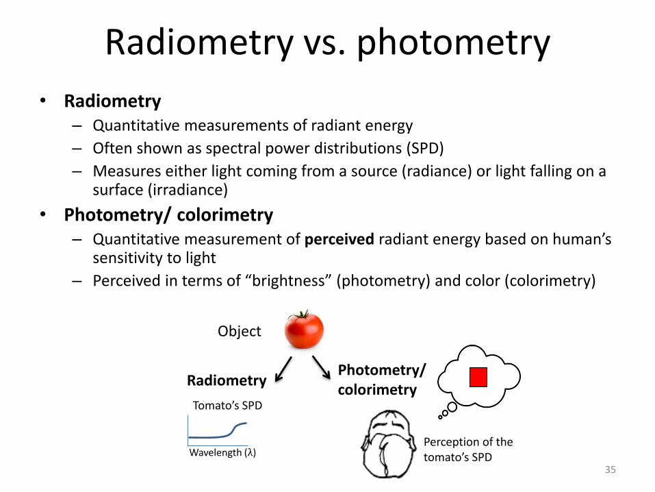
• Radiometry– Quantitative measurements of radiant energy
– Often shown as spectral power distributions (SPD)
– Measures either light coming from a source (radiance) or light falling on a surface (irradiance)
• Photometry/ colorimetry– Quantitative measurement of perceived radiant energy based on human’s
sensitivity to light
– Perceived in terms of “brightness” (photometry) and color (colorimetry)
Wavelength (λ)
RadiometryPhotometry/colorimetry
Tomato’s SPD
Perception of thetomato’s SPD
Object
35
Quantifying color
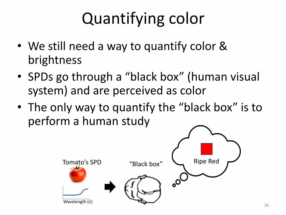
• We still need a way to quantify color & brightness
• SPDs go through a “black box” (human visual system) and are perceived as color
• The only way to quantify the “black box” is to perform a human study
Wavelength (λ)
“Black box”Tomato’s SPD Ripe Red
36

Experiments for photometryReference bright light with fixed radiant power.
Chromatic source light ata particular wavelength andadjustable radiant power.
Alternate between the source light andreference light 17 times per second (17 hz).A flicker will be noticeable unless the twolights have the same perceived “brightness”.
The viewer adjusts the radiant power of thechromatic light until the flicker disappears(i.e. the lights fuse into a constant color).The amount of radiant power needed for thisfusion to happen is recorded.
Repeat this flicker fusion test for each wave-length in the source light. This allows method can be used to determine the perceived “brightness” of each wavelength.
The “flicker photometry”experiment for photopicsensitivity.
+
(Alternating between source and reference @ 17Hz)
450nm 600nm 650nmRel
ativ
e P
ow
er
Viewer graduallyincreases sourceradiant power
37
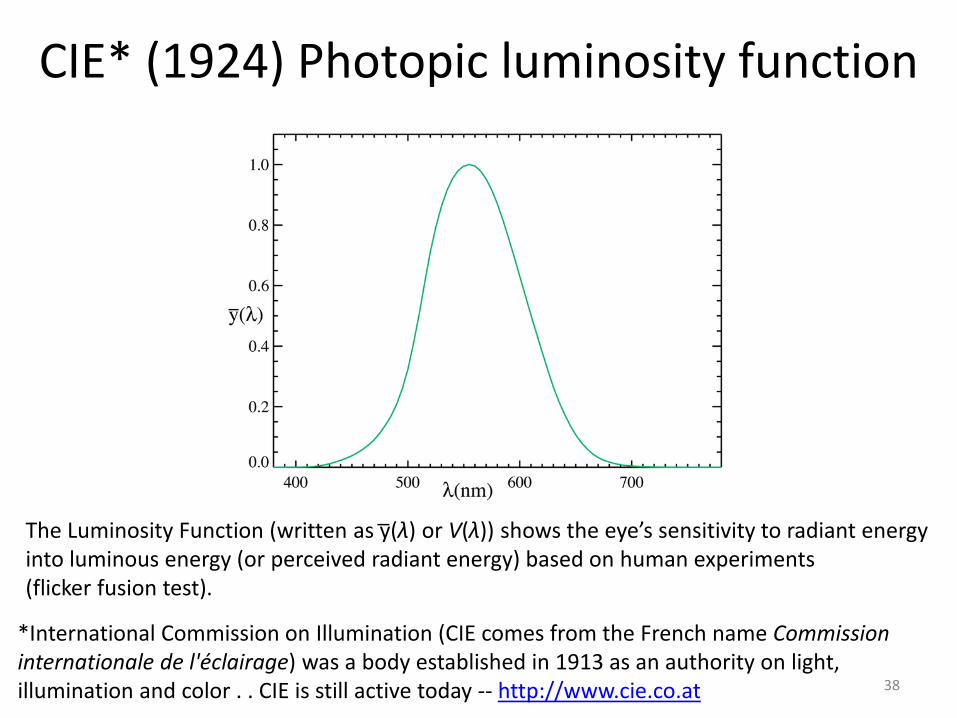
CIE* (1924) Photopic luminosity function
*International Commission on Illumination (CIE comes from the French name Commission internationale de l'éclairage) was a body established in 1913 as an authority on light, illumination and color . . CIE is still active today -- http://www.cie.co.at
The Luminosity Function (written as y(λ) or V(λ)) shows the eye’s sensitivity to radiant energy into luminous energy (or perceived radiant energy) based on human experiments (flicker fusion test).
_
38

Colorimetry
• Based on tristimulus color theory, colorimetry attempts to quantify all visible colors in terms of a standard set of primaries
= R1 + G1 + B1
Three fixed primariesTarget color
39
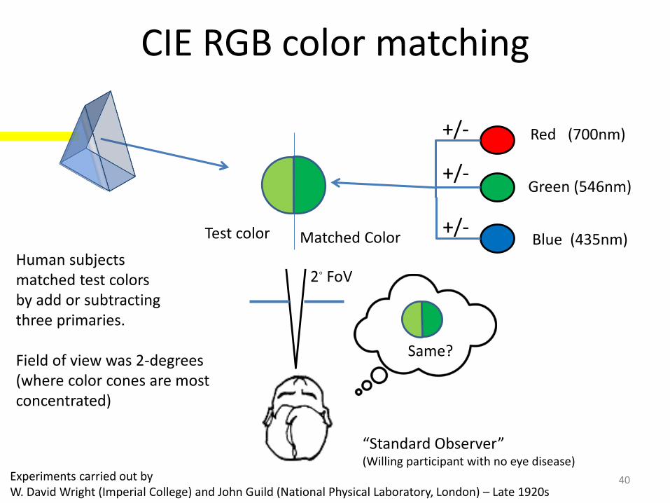
CIE RGB color matching
Test color Matched Color
Red (700nm)
Green (546nm)
Blue (435nm)
+/-
+/-
+/-
“Standard Observer”(Willing participant with no eye disease)
Human subjectsmatched test colors by add or subtracting three primaries.
Field of view was 2-degrees(where color cones are mostconcentrated)
Same?
2◦ FoV
Experiments carried out byW. David Wright (Imperial College) and John Guild (National Physical Laboratory, London) – Late 1920s
40

CIE RGB color matching
For some test colors, nomix of the primaries couldgive a match! For these cases,the subjects were ask to add primaries to the test color to make the match.
This was treated as a negativevalue of the primary added tothe test color.
Test color Matched Color
Red (700nm)
Green (546nm)
Blue (435nm)
“Standard Observer”(Willing participant with no eye disease)
Same?
2◦ FoV
+/-
+/-
+/-
+
41
Primary is added to the test color!
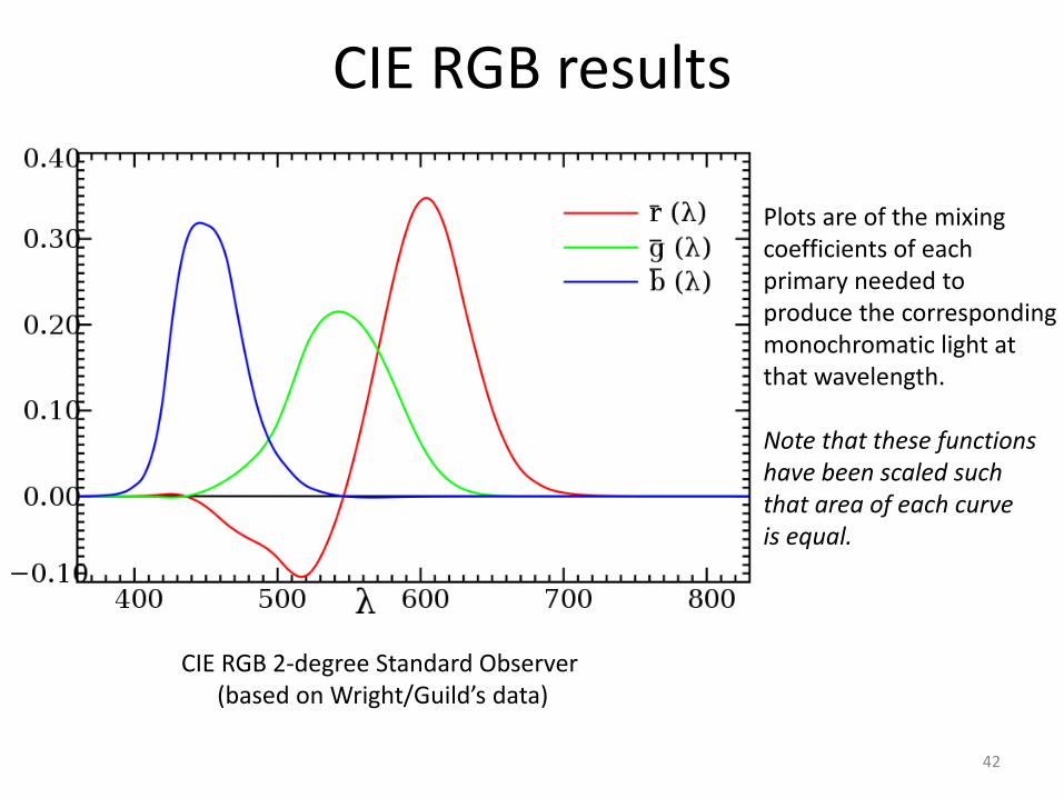
CIE RGB results
CIE RGB 2-degree Standard Observer (based on Wright/Guild’s data)
Plots are of the mixingcoefficients of eachprimary needed to produce the corresponding monochromatic light at that wavelength.
Note that these functionshave been scaled suchthat area of each curveis equal.
42

CIE RGB results
Negative points, the primary used did notspan the full range of perceptual color.
43
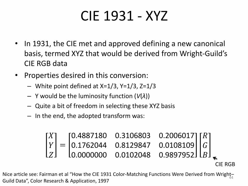
CIE 1931 - XYZ
• In 1931, the CIE met and approved defining a new canonical basis, termed XYZ that would be derived from Wright-Guild’s CIE RGB data
• Properties desired in this conversion:– White point defined at X=1/3, Y=1/3, Z=1/3
– Y would be the luminosity function (V(λ))
– Quite a bit of freedom in selecting these XYZ basis
– In the end, the adopted transform was:
𝑋𝑌𝑍=
0.4887180 0.3106803 0.20060170.1762044 0.8129847 0.01081090.0000000 0.0102048 0.9897952
𝑅𝐺𝐵
Nice article see: Fairman et al “How the CIE 1931 Color-Matching Functions Were Derived from Wright–Guild Data”, Color Research & Application, 1997
CIE RGB
44

CIE XYZ
This shows the mixing coefficients x(λ), y(λ), z(λ) for the CIE 1931 2-degree standardobserver XYZ basis computed from the CIE RGB data. Coefficients are all now positive. Note that the basis XYZ are not physical SPD like in CIE RGB, but linear combinations defined by the matrix on the previous slide.
_ _ _
45
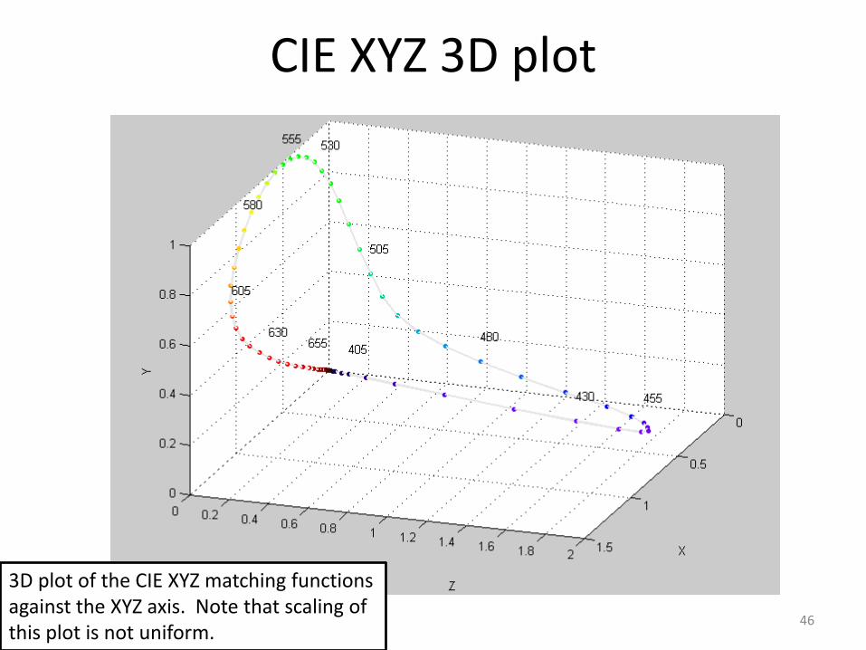
CIE XYZ 3D plot
3D plot of the CIE XYZ matching functionsagainst the XYZ axis. Note that scaling ofthis plot is not uniform.
46

What does it mean?
• We now have a canonical color space to describe SPDs
• Given an SPD, I(λ), we can find its mapping into the CIE XYZ space
• Given two SPDs, if their CIE XYZ values are equal, then they are considered the same perceived color, i.e.– I1 (λ), I2 (λ) → (X1, Y1, Z1) = (X2, Y2, Z2) [ perceived as the same color ]
• So . . we can quantitatively describe color!
𝑋 =
380
780
𝐼(λ) 𝑥(λ) ⅆλ 𝑌 =
380
780
𝐼(λ) 𝑦 (λ) ⅆλ 𝑍 =
380
780
𝐼(λ) 𝑧(λ)ⅆλ
47
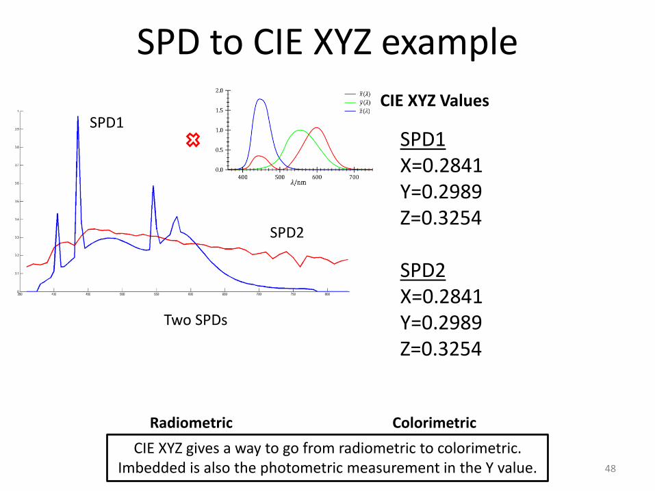
SPD to CIE XYZ example
Two SPDs
SPD1
SPD2
SPD1X=0.2841Y=0.2989Z=0.3254
SPD2X=0.2841Y=0.2989Z=0.3254
From their CIE XYZmappings, we can determinethat these twoSPDs will be perceived as thesame color (evenwithout needingto see the color!)
Thanks CIE XYZ!
CIE XYZ Values
Radiometric Colorimetric
CIE XYZ gives a way to go from radiometric to colorimetric.Imbedded is also the photometric measurement in the Y value. 48

What does it mean?
• CIE XYZ space is also considered “device independent” – the XYZ values are not specific to any device
• Devices (e.g. cameras, flatbed, scanners, printers, displays) can find mappings of their device specific values to corresponding CIE XYZ values. This provides a canonical space to match between devices (at least in theory)
49
Luminance-chromaticity space (CIE xyY)
• CIE XYZ describes a color in terms of linear combination of three primaries (XYZ)
• Sometimes it is useful to discuss color in terms of luminance (perceived brightness) and chromaticity (we can think of as the hue-saturation combined)
• CIE xyY space is used for this purpose
50
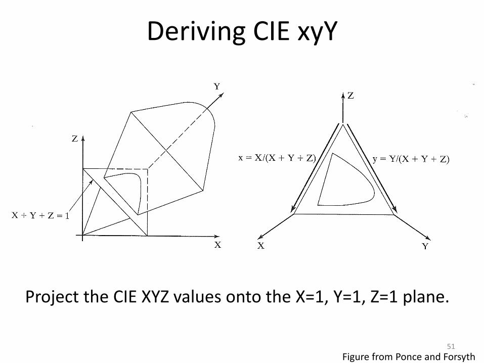
Deriving CIE xyY
Project the CIE XYZ values onto the X=1, Y=1, Z=1 plane.
Figure from Ponce and Forsyth 51
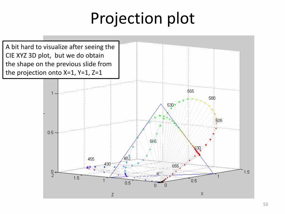
Projection plot
A bit hard to visualize after seeing theCIE XYZ 3D plot, but we do obtain the shape on the previous slide from the projection onto X=1, Y=1, Z=1
52
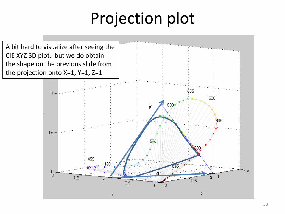
Projection plot
A bit hard to visualize after seeing theCIE XYZ 3D plot, but we do obtain the shape on the previous slide from the projection onto X=1, Y=1, Z=1
x
y
53
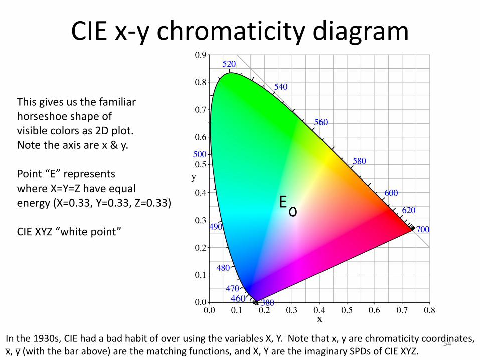
This gives us the familiarhorseshoe shape ofvisible colors as 2D plot.Note the axis are x & y.
E
Point “E” representswhere X=Y=Z have equalenergy (X=0.33, Y=0.33, Z=0.33)
CIE XYZ “white point”
In the 1930s, CIE had a bad habit of over using the variables X, Y. Note that x, y are chromaticity coordinates,x, y (with the bar above) are the matching functions, and X, Y are the imaginary SPDs of CIE XYZ. _ _ 54
CIE x-y chromaticity diagram

CIE x-y chromaticity diagram
Moving along the outsideof the diagram givesthe hues.
Moving way fromthe white pointrepresents more saturation.
55

CIE xyY
• Generally when we use CIE xyY, we only look at the (x,y) values on the 2D diagram of the CIE x-y chromaticity chart
• However, the Y value (the same Y from CIE XYZ) represents the perceived brightness of the color
• With values (x,y,Y) we can reconstruct back to XYZ
𝑋 =𝑌
𝑦𝑥 𝑍 =
𝑌
𝑦(1 − 𝑥 − 𝑦)
56

Fast forward 80+ years
• CIE 1931 XYZ, CIE 1931 xyY (2-degree standard observer) color spaces have stood the test of time
• Many other studies have followed (most notably - CIE 1965 XYZ 10-degree standard observer), . . .
• But in the literature (and in this tutorial) you’ll find CIE 1931 XYZ color space making an appearance often
57

What is perhaps most amazing?
• 80+ years of CIE XYZ is all down to the experiments by the “standard observers”
• How many standard observers were used? 100, 500, 1000?
A Standard Observer
58

CIE XYZ is based on 17 Standard Observers
10 by Wright, 7 by Guild
“The Standard Observers” 59
A caution on CIE x-y chromaticity
From Mark D. Fairchild book: “Color Appearance Models”
“The use of chromaticity diagrams should be avoided in most circumstances, particularly when the phenomena being investigated are highly dependent on the three-dimensional nature of color. For example, the display and comparison of the color gamuts of imaging devices in chromaticity diagrams is misleading to the point of being almost completely erroneous.”
Re-quoted from the Mark Meyer’s “Deconstructing Chromaticity” article.60

We are done with color, right?Almost . . .
61
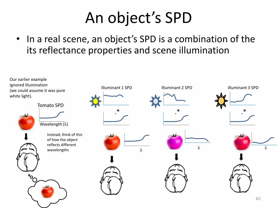
An object’s SPD• In a real scene, an object’s SPD is a combination of the
its reflectance properties and scene illumination
Wavelength (λ)
Tomato SPD
Our earlier exampleignored illumination(we could assume it was purewhite light).
Instead, think of thisof how the objectreflects differentwavelengths
Illuminant 1 SPD
.*
λ
Illuminant 2 SPD
.*
λ
Illuminant 3 SPD
.*
λ
62
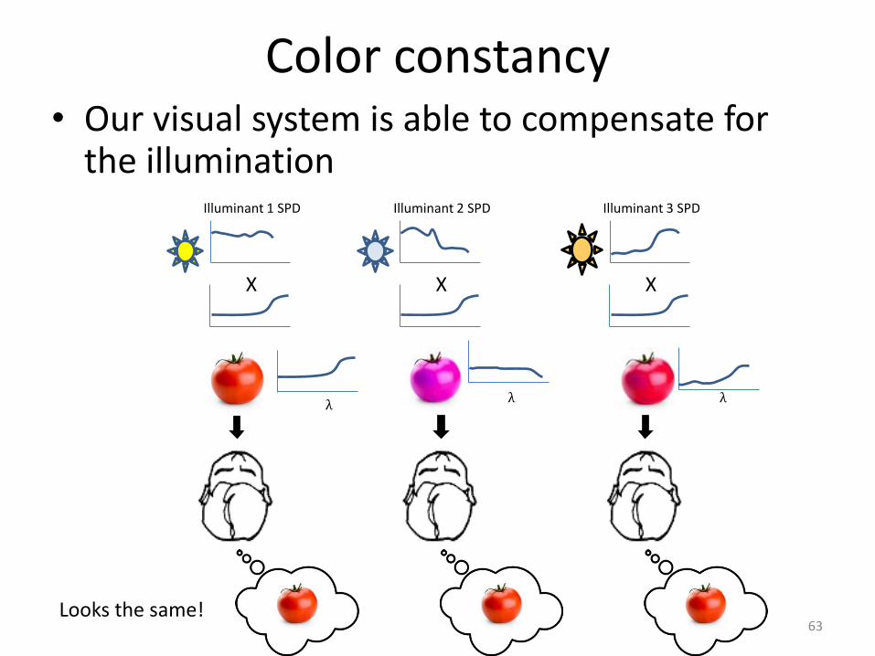
Color constancy• Our visual system is able to compensate for
the illumination Illuminant 1 SPD
X
Illuminant 2 SPD
X
Illuminant 3 SPD
X
λ λ λ
Looks the same!63

Color constancy/chromatic adaptation
• Color constancy, or chromatic adaptation, is the ability of the human visual system to adapt to scene illumination
• This ability is not perfect, but it works fairly well
• Image sensors do not have this ability (it must be performed as a processing step, i.e. “white balance”)
• Note: Our eyes do not adjust to the lighting in the photograph -- we adjust to the viewing conditions of the scene we are viewing the photograph in!
64
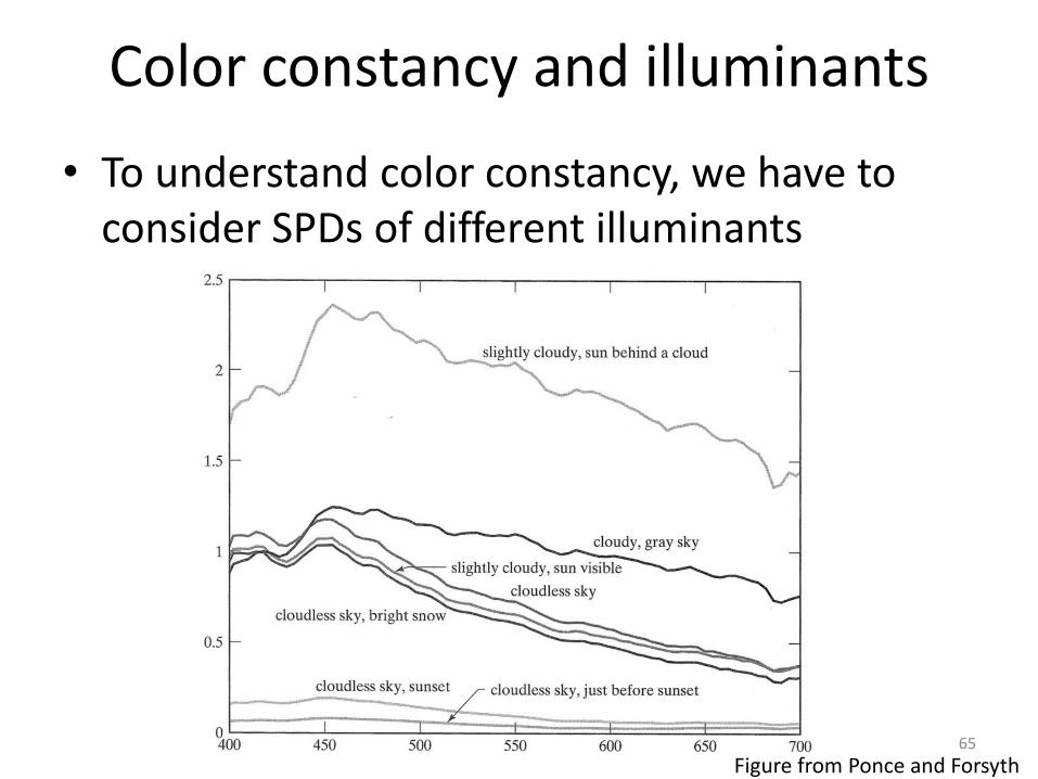
Color constancy and illuminants
• To understand color constancy, we have to consider SPDs of different illuminants
Figure from Ponce and Forsyth 65
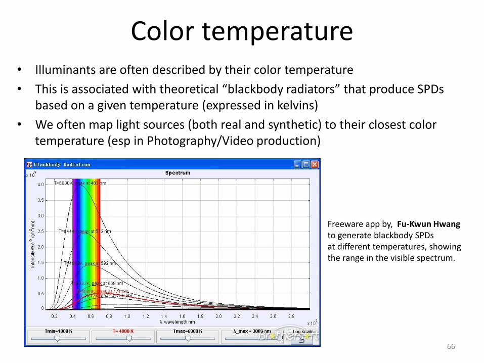
Color temperature• Illuminants are often described by their color temperature
• This is associated with theoretical “blackbody radiators” that produce SPDs based on a given temperature (expressed in kelvins)
• We often map light sources (both real and synthetic) to their closest color temperature (esp in Photography/Video production)
Freeware app by, Fu-Kwun Hwangto generate blackbody SPDsat different temperatures, showingthe range in the visible spectrum.
66

Color temperature
From B&H Photo
Typical description ofcolor temperature usedin photography & lightingsources.
67
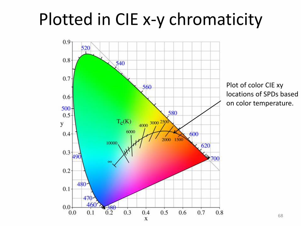
Plotted in CIE x-y chromaticity
Plot of color CIE xylocations of SPDs basedon color temperature.
68
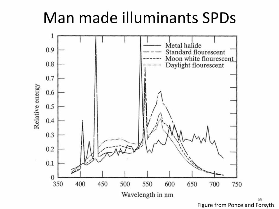
Man made illuminants SPDs
Figure from Ponce and Forsyth 69
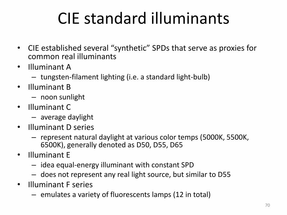
CIE standard illuminants
• CIE established several “synthetic” SPDs that serve as proxies for common real illuminants
• Illuminant A – tungsten-filament lighting (i.e. a standard light-bulb)
• Illuminant B– noon sunlight
• Illuminant C – average daylight
• Illuminant D series– represent natural daylight at various color temps (5000K, 5500K,
6500K), generally denoted as D50, D55, D65
• Illuminant E– idea equal-energy illuminant with constant SPD– does not represent any real light source, but similar to D55
• Illuminant F series– emulates a variety of fluorescents lamps (12 in total)
70

CIE standard illuminants
D, E, and F series images from http://www.image-engineering.de
SPDs for CIE standard illuminant A, B, C SPDs for CIE standard illuminant D50, D55, D65
SPDs for CIE standard illuminant E SPDs for CIE standard illuminants F2, F8, F11
71

White point
• A white point is a CIE XYZ or CIE xyY value of an ideal “white target” or “white reference”
• This is essentially an illuminants SPD in terms of CIE XYZ/CIE xyY
– We can assume the white reference is reflecting the illuminant
• The idea of chromatic adaptation is to make white points the same between scenes
72

White points in CIE x-y chromaticity
C
D65
B
A
E
CIE IlluminantsA, B, C, D65, E in terms of CIE x-y
CIE x , yA 0.44757 , 0.40745B 0.34842 , 0.35161C 0.31006 , 0.31616D65 0.31271 , 0.32902E 0.33333 , 0.33333
73
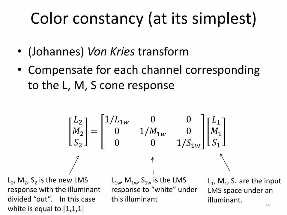
Color constancy (at its simplest)
• (Johannes) Von Kries transform
• Compensate for each channel corresponding to the L, M, S cone response
𝐿2𝑀2𝑆2
=
1/𝐿1𝑤 0 00 1/𝑀1𝑤 00 0 1/𝑆1𝑤
𝐿1𝑀1𝑆1
L1, M1, S1 are the inputLMS space under anilluminant.
L1w, M1w, S1w is the LMSresponse to “white” underthis illuminant
L2, M2, S2 is the new LMSresponse with the illuminantdivided “out”. In this casewhite is equal to [1,1,1]
74
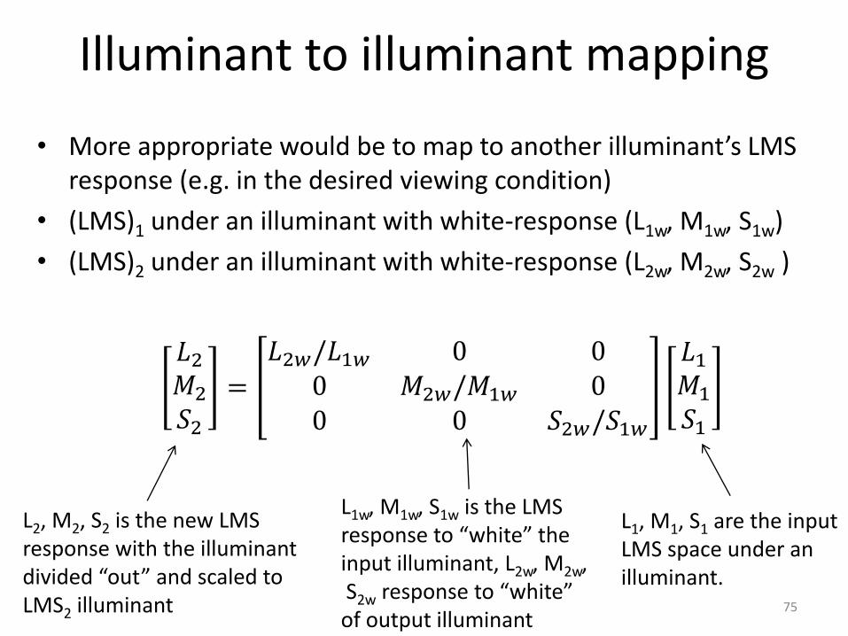
Illuminant to illuminant mapping
• More appropriate would be to map to another illuminant’s LMS response (e.g. in the desired viewing condition)
• (LMS)1 under an illuminant with white-response (L1w, M1w, S1w)
• (LMS)2 under an illuminant with white-response (L2w, M2w, S2w )
𝐿2𝑀2𝑆2
=
𝐿2𝑤/𝐿1𝑤 0 00 𝑀2𝑤/𝑀1𝑤 00 0 𝑆2𝑤/𝑆1𝑤
𝐿1𝑀1𝑆1
L1, M1, S1 are the inputLMS space under anilluminant.
L1w, M1w, S1w is the LMSresponse to “white” theinput illuminant, L2w, M2w,S2w response to “white”of output illuminant
L2, M2, S2 is the new LMSresponse with the illuminantdivided “out” and scaled toLMS2 illuminant 75

Example
Simulation of different “white points” by photographing a “white” object under different illumination.
Images courtesy of Sharon Albert (Weizmann Institute)76

Example
Input
Adapted to“target” illuminant
Before After Before After Target Illumination
Here, we have mapped the two input images to one belowto mimic chromatic adaptation.The “white” part of the cup isshown before and after to helpshow that the illumination fallingon white appears similar afterthe “chromatic adaptation”.
77

Now we are finally done with color?Almost (really) . . .
78
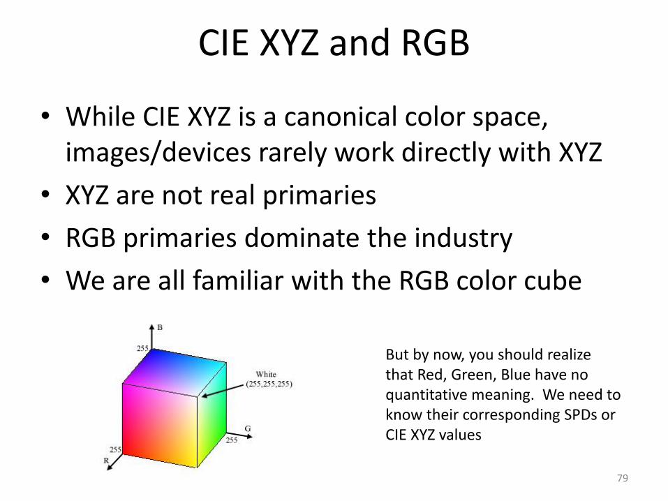
CIE XYZ and RGB
• While CIE XYZ is a canonical color space, images/devices rarely work directly with XYZ
• XYZ are not real primaries
• RGB primaries dominate the industry
• We are all familiar with the RGB color cube
But by now, you should realizethat Red, Green, Blue have no quantitative meaning. We need to know their corresponding SPDs orCIE XYZ values
79
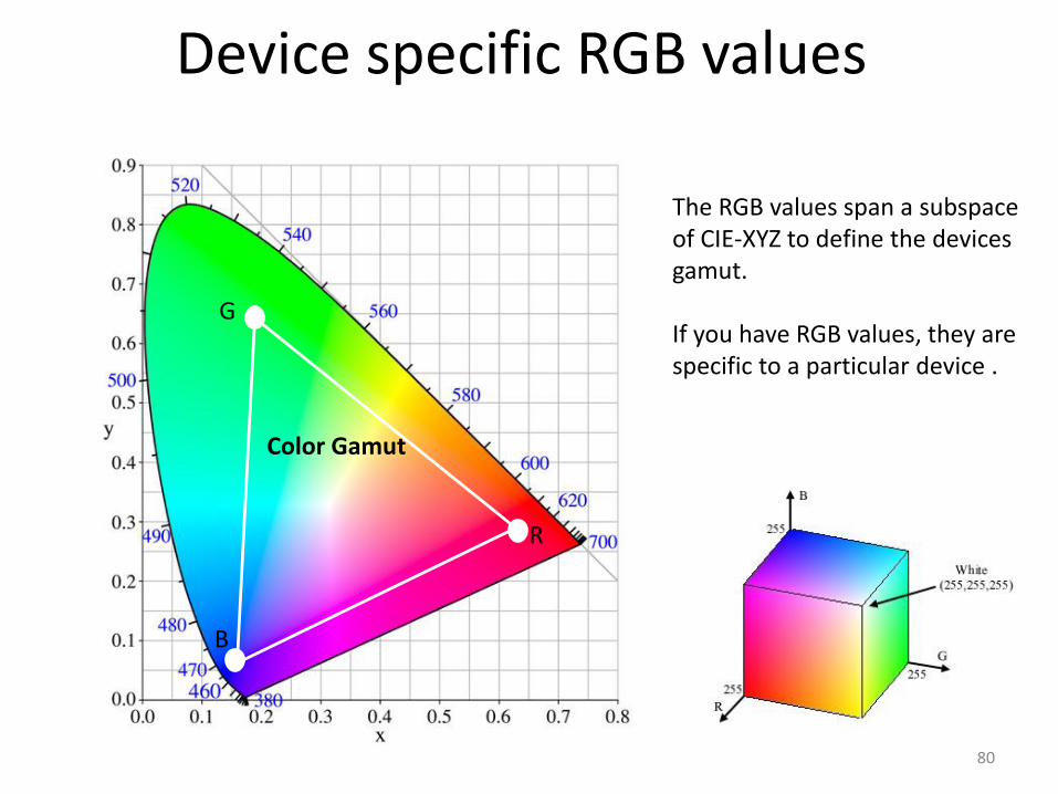
Device specific RGB values
R
G
B
Color Gamut
The RGB values span a subspaceof CIE-XYZ to define the devicesgamut.
If you have RGB values, they arespecific to a particular device .
80
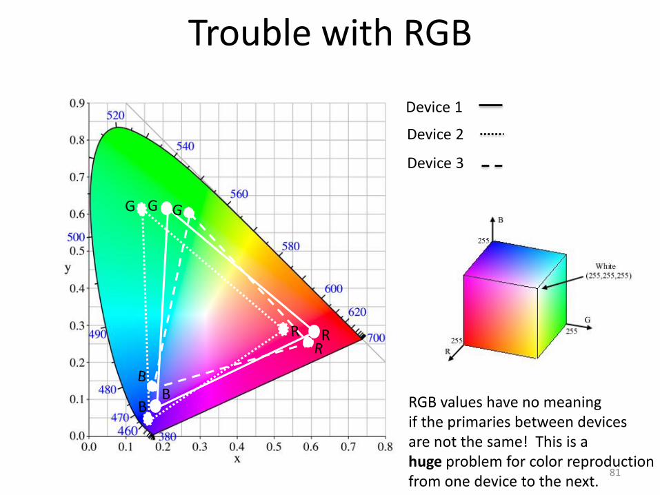
Trouble with RGB
R
G
B
Device 1
Device 2
Device 3
RGB values have no meaningif the primaries between devicesare not the same! This is a huge problem for color reproductionfrom one device to the next.
81

Standard RGB (sRGB)
R
G
In 1996, Microsoft and HP defined a set of “standard” RGB primaries.R=CIE xyY (0.64, 0.33, 0.2126)G=CIE xyY (0.30, 0.60, 0.7153)B=CIE xyY (0.15, 0.06, 0.0721)
This was considered an RGBspace achievable by most devices at the time.
White point was set to the D65illuminant. This is an importantthing to note. It means sRGBhas built in the assumedviewing condition (6500K daylight).82
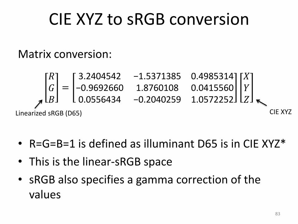
CIE XYZ to sRGB conversion
Matrix conversion:
• R=G=B=1 is defined as illuminant D65 is in CIE XYZ*
• This is the linear-sRGB space
• sRGB also specifies a gamma correction of the values
𝑅𝐺𝐵=
3.2404542 −1.5371385 0.4985314−0.9692660 1.8760108 0.04155600.0556434 −0.2040259 1.0572252
𝑋𝑌𝑍
CIE XYZLinearized sRGB (D65)
83
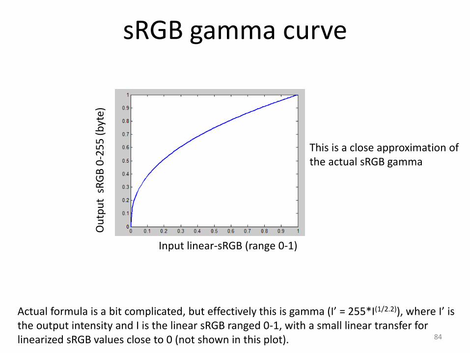
sRGB gamma curve
Input linear-sRGB (range 0-1)
Ou
tpu
t s
RG
B 0
-25
5 (
byt
e)
Actual formula is a bit complicated, but effectively this is gamma (I’ = 255*I(1/2.2)), where I’ is the output intensity and I is the linear sRGB ranged 0-1, with a small linear transfer for linearized sRGB values close to 0 (not shown in this plot).
This is a close approximation ofthe actual sRGB gamma
84
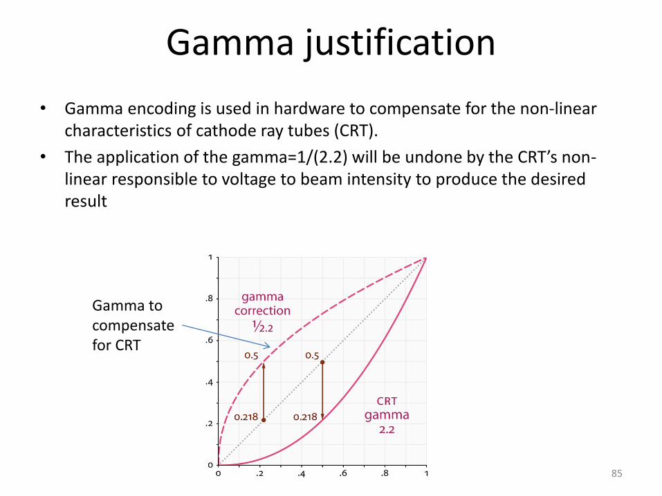
Gamma justification
• Gamma encoding is used in hardware to compensate for the non-linear characteristics of cathode ray tubes (CRT).
• The application of the gamma=1/(2.2) will be undone by the CRT’s non-linear responsible to voltage to beam intensity to produce the desired result
Gamma to compensatefor CRT
85
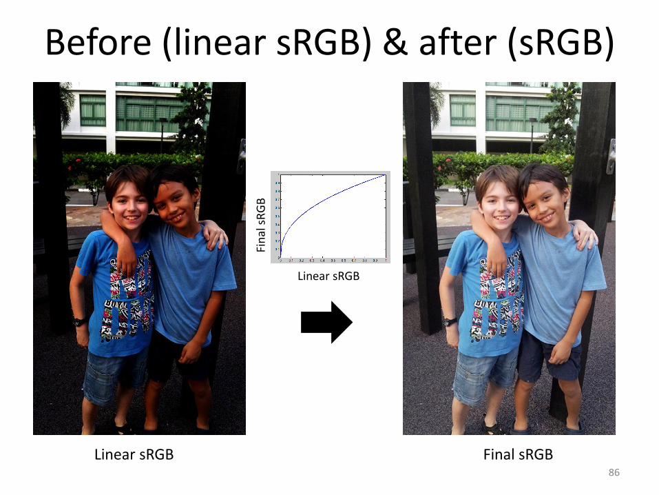
Before (linear sRGB) & after (sRGB)
Linear sRGB Final sRGB
Linear sRGBFi
nal
sR
GB
86
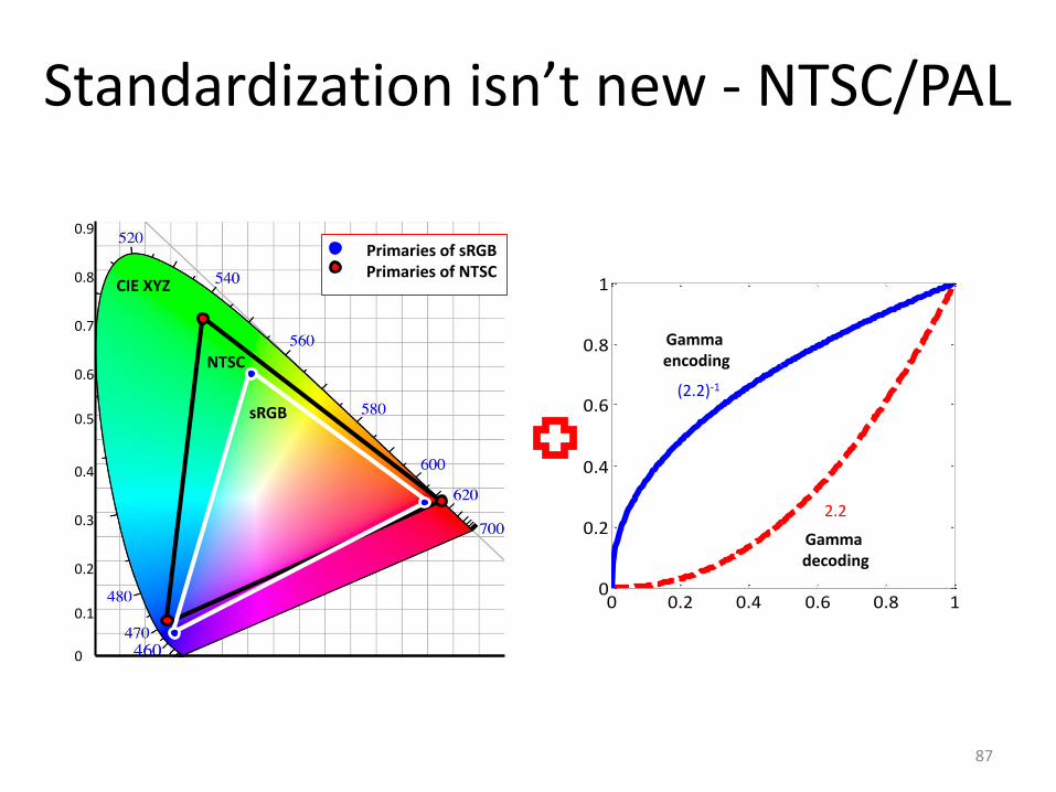
Standardization isn’t new - NTSC/PAL
0 0.2 0.4 0.6 0.8 10
0.2
0.4
0.6
0.8
1
NTSC
0
0.9
0.6
0.7
0.5
0.4
0.3
0.2
0.1
0.8CIE XYZ
sRGB
Gamma encoding
Primaries of sRGBPrimaries of NTSC
2.2
(2.2)-1
Gamma decoding
87
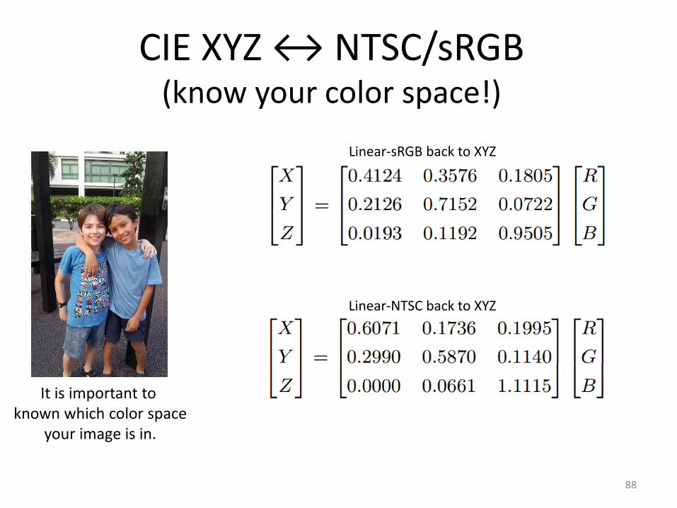
CIE XYZ ↔ NTSC/sRGB(know your color space!)
Linear-sRGB back to XYZ
Linear-NTSC back to XYZ
It is important to known which color space
your image is in.
88

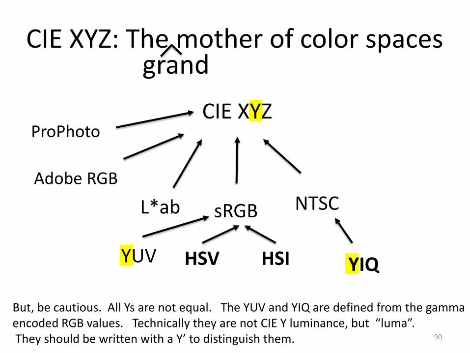
CIE XYZ: The mother of color spaces
CIE XYZ
L*ab sRGB NTSC
ProPhoto
Adobe RGB
YIQHSV HSI
grand
89
YUV
CIE XYZ: The mother of color spacesgrand
But, be cautious. All Ys are not equal. The YUV and YIQ are defined from the gamma encoded RGB values. Technically they are not CIE Y luminance, but “luma”. They should be written with a Y’ to distinguish them. 90
CIE XYZ
L*ab sRGB NTSC
ProPhoto
Adobe RGB
YIQHSV HSIYUV
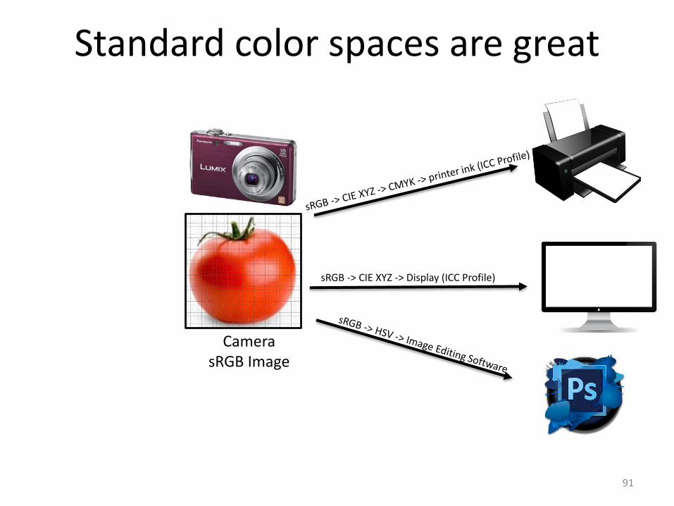
Standard color spaces are great
CamerasRGB Image
sRGB -> CIE XYZ -> Display (ICC Profile)
91

Benefits of sRGB
• Like CIE XYZ, sRGB is a device independent color space (often called an output color space)
• If you have two pixels with the same sRGB values, they will have the same CIE XYZ value, which means “in theory” they will appear as the same perceived value
• Does this happen in practice?
92
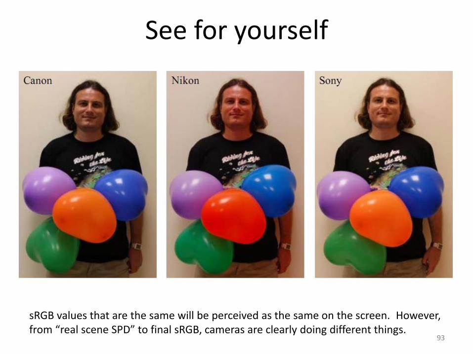
See for yourself
sRGB values that are the same will be perceived as the same on the screen. However,from “real scene SPD” to final sRGB, cameras are clearly doing different things.
93

Congratulations!
You
26 June 2016
“Crash Course on Color”
94

Crash course on color is over!
• A lot of information to absorb
• Understanding colorimetry is required to understand imaging devices
• CIE XYZ and CIE illuminants will make many appearances in color imaging/processing discussions
95
Tutorial schedule
• Part 1 (General Part)
– Motivation
– Review of color/color spaces
– Overview of camera imaging pipeline
• Part 2 (Specific Part)
– Modeling the in-camera color pipeline
– Photo-refinishing
• Part 3 (Wrap Up)
– The good, the bad, and the ugly of commodity cameras and computer vision research
– Concluding Remarks
96
Overview of the Camera Imaging Pipeline
97
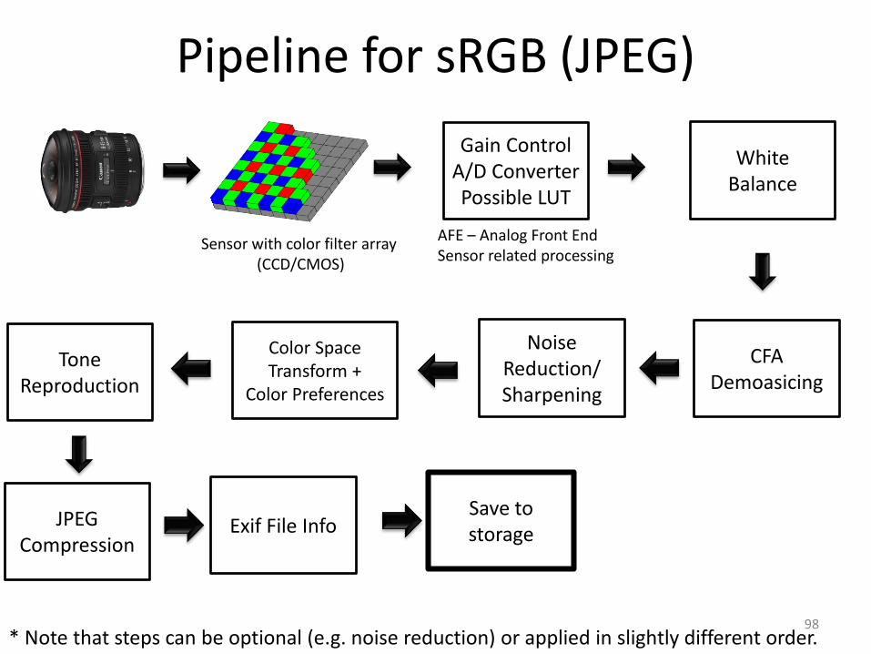
Pipeline for sRGB (JPEG)
Gain ControlA/D ConverterPossible LUT
AFE – Analog Front EndSensor related processing
Sensor with color filter array (CCD/CMOS)
CFADemoasicing
White Balance
Color Space Transform +
Color Preferences
Tone Reproduction
JPEG Compression
Exif File Info
Noise Reduction/Sharpening
Save to storage
* Note that steps can be optional (e.g. noise reduction) or applied in slightly different order.98
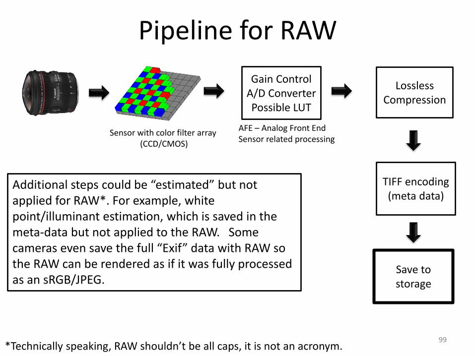
Pipeline for RAW
Lossless Compression
TIFF encoding(meta data)
Additional steps could be “estimated” but not applied for RAW*. For example, white point/illuminant estimation, which is saved in the meta-data but not applied to the RAW. Some cameras even save the full “Exif” data with RAW so the RAW can be rendered as if it was fully processed as an sRGB/JPEG.
Save to storage
Gain ControlA/D ConverterPossible LUT
AFE – Analog Front EndSensor related processing
*Technically speaking, RAW shouldn’t be all caps, it is not an acronym.
Sensor with color filter array (CCD/CMOS)
99
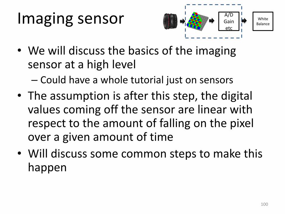
Imaging sensor
• We will discuss the basics of the imaging sensor at a high level– Could have a whole tutorial just on sensors
• The assumption is after this step, the digital values coming off the sensor are linear with respect to the amount of falling on the pixel over a given amount of time
• Will discuss some common steps to make this happen
A/DGainetc
White Balance
100
Imaging sensor A/DGainetc
White Balance
Sensor
Color Filter
Sensor
Color Filter
Sensor
Color Filter
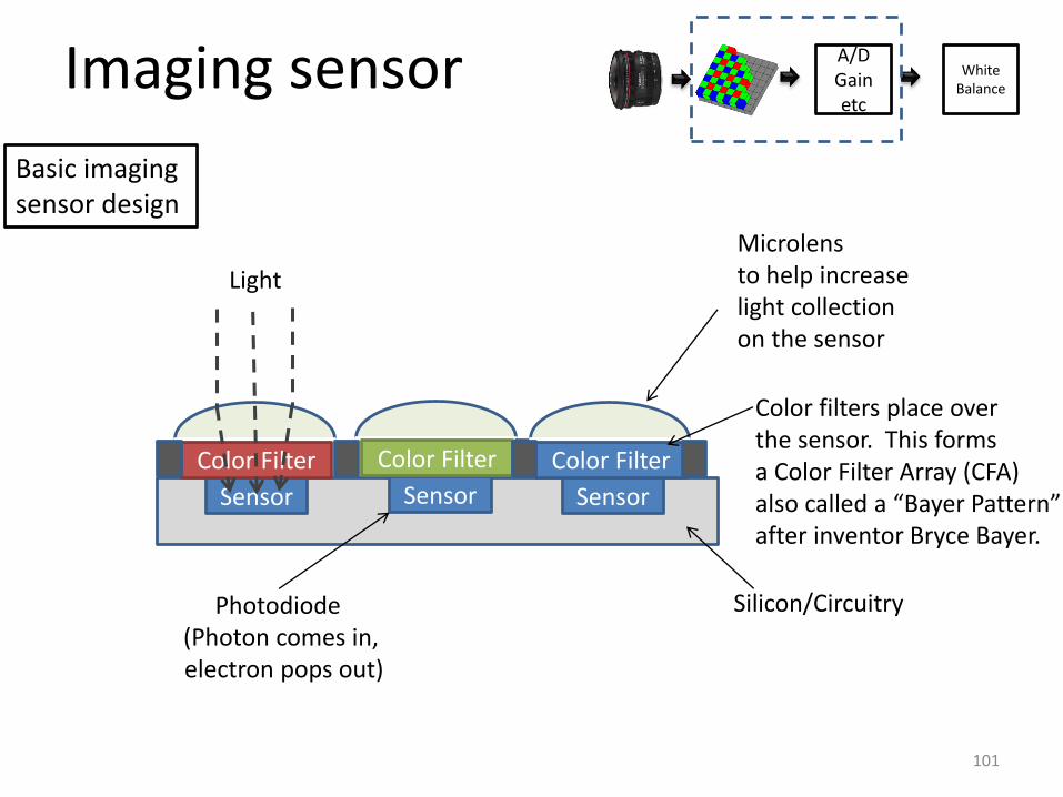
Basic imaging sensor design
Microlensto help increaselight collectionon the sensor
Light
Photodiode (Photon comes in,electron pops out)
Silicon/Circuitry
Color filters place overthe sensor. This formsa Color Filter Array (CFA)also called a “Bayer Pattern”after inventor Bryce Bayer.
101
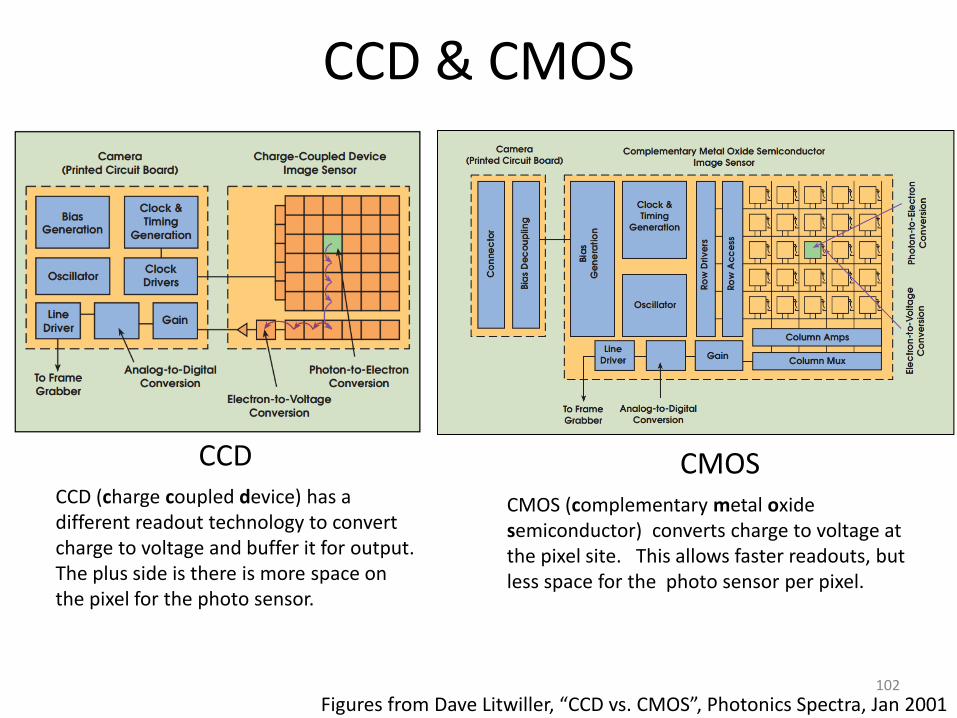
CCD & CMOS
CCD CMOS
Figures from Dave Litwiller, “CCD vs. CMOS”, Photonics Spectra, Jan 2001
CCD (charge coupled device) has a different readout technology to convertcharge to voltage and buffer it for output.The plus side is there is more space on the pixel for the photo sensor.
CMOS (complementary metal oxide semiconductor) converts charge to voltage at the pixel site. This allows faster readouts, but less space for the photo sensor per pixel.
102

Camera RGB sensitivity
• The color filter array (CFA) on the camera filters the light into three primaries
Plotted from camera sensitivity database by Dr. Jinwei Gu from Rochester Institute of Technology (RIT)http://www.cis.rit.edu/jwgu/research/camspec/ 103
Black light subtraction
• Sensor values for pixels with “no light” should be zero
• But, often, this is not the case for various reasons– Cross talk on the sensor, etc. .
– This can also change with sensor temperature
• This can be corrected by capturing a set of pixels that do not see light
• Place a dark-shield around sensor
• Subtract the level from the “black” pixels
104
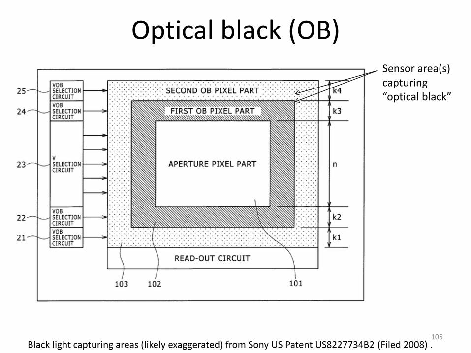
Optical black (OB)
Black light capturing areas (likely exaggerated) from Sony US Patent US8227734B2 (Filed 2008) .
Sensor area(s) capturing“optical black”
105
Signal amplification (gain)
• Imaging sensor signal is amplified
• Amplification to assist A/D
– Need to get the voltage to the range required to the desired digital output
• This gain could also be used to accommodate camera ISO settings
– Unclear if all cameras do this here or use a simple post-processing gain to the RAW for ISO settings
– DSLR cameras RAW is modified by the ISO setting
106
Defective pixel mask
• CCD/CMOS have pixels that are defective
• Dead pixel masks are pre-calibrated at the factory
– Using “dark current” calibration
– Take an image with no light
– Record locations reporting values to make “mask”
• Bad pixels in the mask are interpolated
• This process seems to happen before RAW is saved
– If you see dead pixels in RAW, these are generally new dead pixels that have appeared after leaving the factory
107
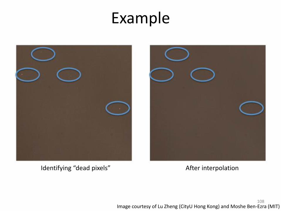
Example
Identifying “dead pixels” After interpolation
Image courtesy of Lu Zheng (CityU Hong Kong) and Moshe Ben-Ezra (MIT)108

Nonlinear response correction
• Some image sensor (generally CMOS) often have a non-linear response to different amounts of irradiance
• A non-linear adjustment or look up table (LUT) interpolation can be used to correct this
109

Other possible distortion correction
• Sensor readout could have spatial distortion for various reasons, e.g. sensor cross-talk
• For point-and-shoot/mobile cameras with fixed lens, vignetting correction for lens distortion could be applied
• Such corrections can be applied using a LUT or polynomial function (in the case of vignetting)
110
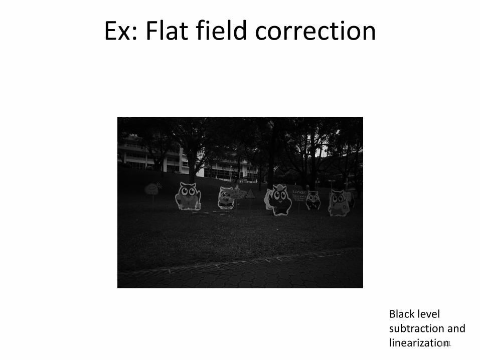
Ex: Flat field correction
Black level subtraction andlinearization111

Ex: Flat field correction(non-uniform gain)
112
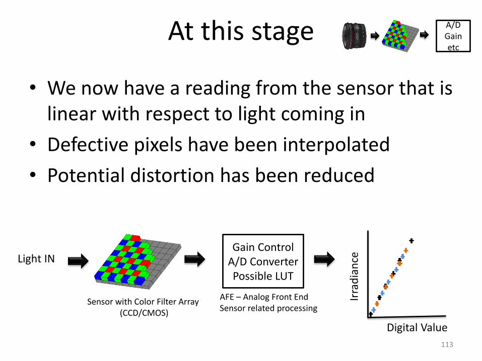
At this stage
• We now have a reading from the sensor that is linear with respect to light coming in
• Defective pixels have been interpolated
• Potential distortion has been reduced
Gain ControlA/D ConverterPossible LUT
AFE – Analog Front EndSensor related processing
Sensor with Color Filter Array (CCD/CMOS)
Light IN
Digital Value
Irra
dia
nce
A/DGainetc
113
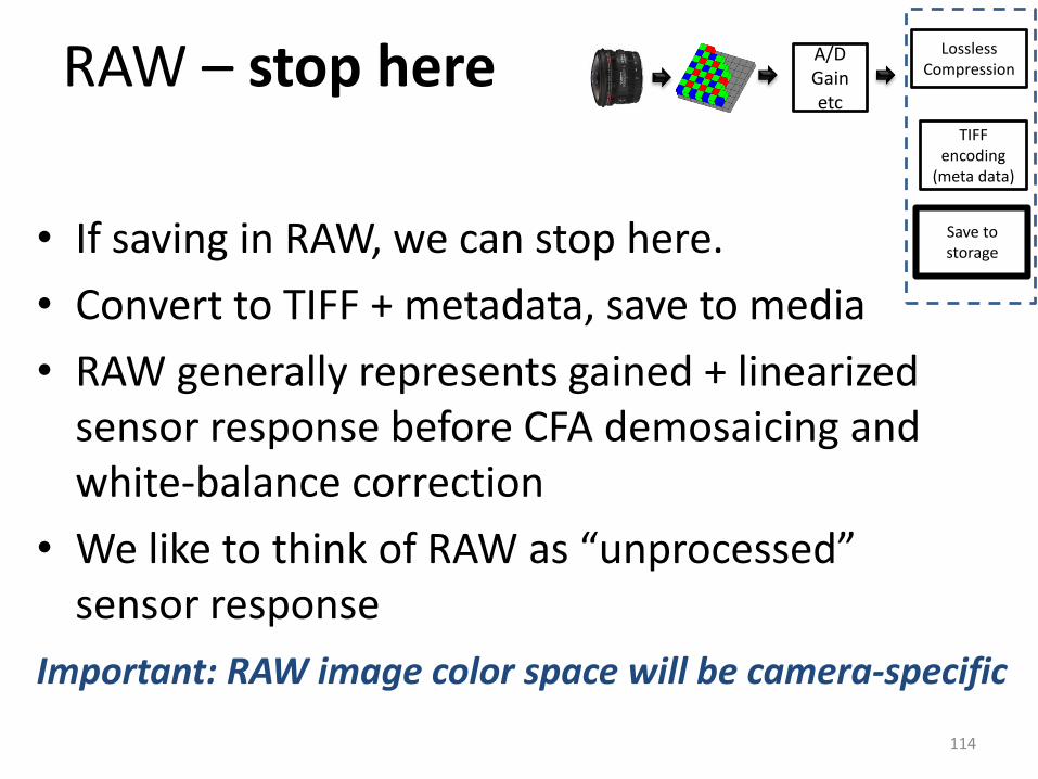
RAW – stop here
• If saving in RAW, we can stop here.
• Convert to TIFF + metadata, save to media
• RAW generally represents gained + linearizedsensor response before CFA demosaicing and white-balance correction
• We like to think of RAW as “unprocessed” sensor response
A/DGainetc
Lossless Compression
TIFF encoding
(meta data)
Save to storage
114
Important: RAW image color space will be camera-specific
White balance
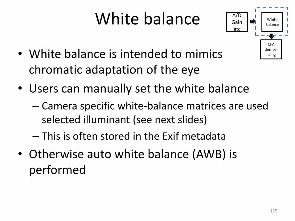
• White balance is intended to mimics chromatic adaptation of the eye
• Users can manually set the white balance
– Camera specific white-balance matrices are used selected illuminant (see next slides)
– This is often stored in the Exif metadata
• Otherwise auto white balance (AWB) is performed
A/DGainetc
White Balance
CFAdemos-
acing
115
WB manual settings
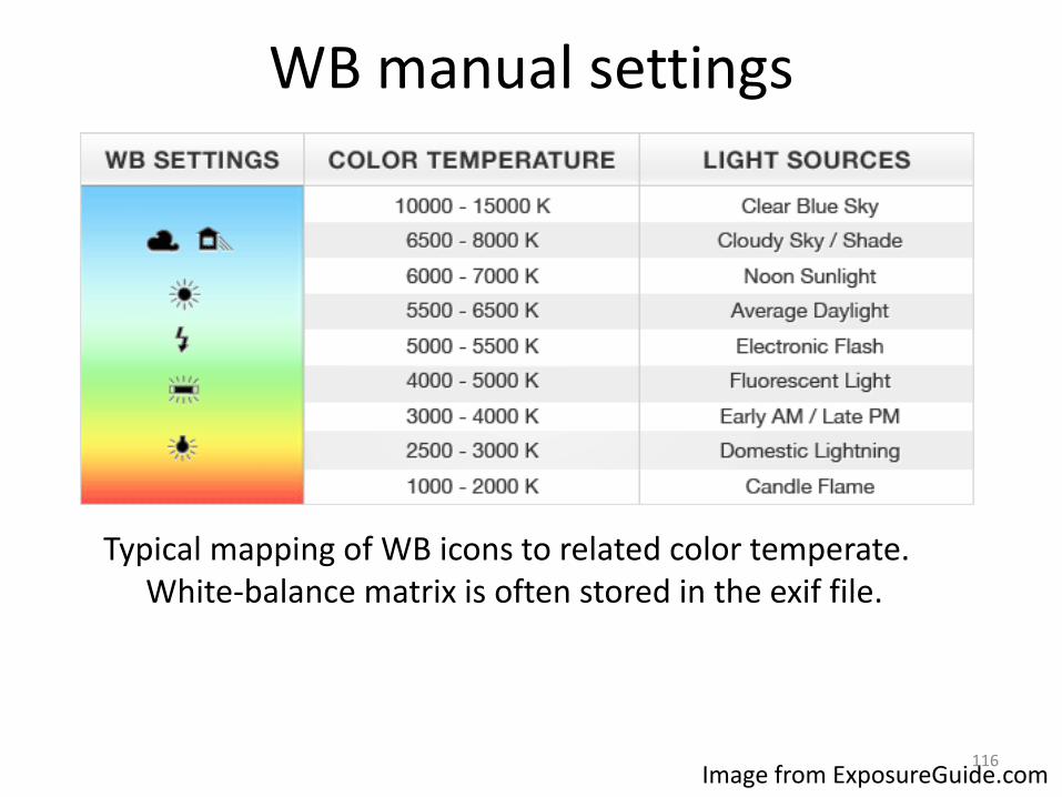
Typical mapping of WB icons to related color temperate. White-balance matrix is often stored in the exif file.
Image from ExposureGuide.com116
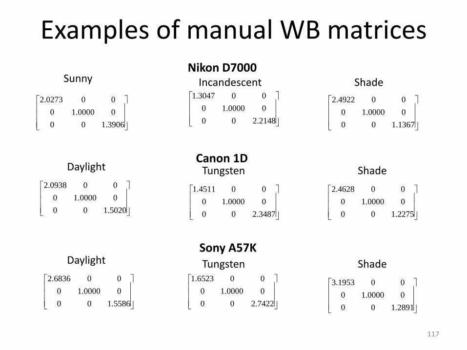
Examples of manual WB matricesNikon D7000
Canon 1D
Sony A57K
Sunny Incandescent Shade
Daylight Tungsten Shade
Daylight Tungsten Shade
1.390600
01.00000
00 2.0273
2.214800
01.00000
001.3047
1.136700
01.00000
002.4922
1.502000
01.00000
002.0938
2.348700
01.00000
001.4511
1.227500
01.00000
002.4628
1.558600
01.00000
002.6836
2.742200
01.00000
001.6523
1.289100
01.00000
003.1953
117
Auto white balance (AWB)
• If manual white balance is not used, then an AWB algorithm is performed
• This is not entirely the same as chromatic adaptation, because it doesn’t have a target illuminant, instead AWB (as the name implies) attempts to make what is assumed to be white map to “pure white”
• Next slides introduce two well known methods: “Gray World” and “White Patch”
118

AWB: Gray world algorithm
• This methods assumes that average reflectance of a scene is achromatic (i.e. gray) – Gray is just the white point not at its brightest, so it serves as an
estimate of the illuminant
– This means that image average should have equal energy, i.e. R=G=B
• Based on this assumption, the algorithm adjusts the input average to be gray as follows:
𝑅𝑎𝑣𝑔 =1
𝑁𝑟 𝑅𝑠𝑒𝑛𝑠𝑜𝑟(r) 𝐺𝑎𝑣𝑔 =
1
𝑁𝑔 𝐺𝑠𝑒𝑛𝑠𝑜𝑟(g) 𝐵𝑎𝑣𝑔 =
1
𝑁𝑏 𝐵𝑠𝑒𝑛𝑠𝑜𝑟(b)
r = red pixels values, g=green pixels values, b =blue pixels valuesNr = # of red pixels, Ng = # of green pixels, Nb = # blue pixels
First, estimate the average response:
Note: # of pixel per channel may be different if white balance is applied to the RAW image before demosaicing. Some pipelines may also transform into another colorspace, e.g. LMS, to perform the white-balance procedure.
119

AWB: Gray world algorithm
• Based on averages, white balance can be expressed as a matrix as:
𝑅′𝐺′𝐵′
=
𝐺𝑎𝑣𝑔/𝑅𝑎𝑣𝑔 0 0
0 1 00 0 𝐺𝑎𝑣𝑔/𝐵𝑎𝑣𝑔
𝑅𝐺𝐵
Sensor RGBWhite-balancedsensor RGB
Matrix scales each channel by its average and then normalizes to the green channel average.
Note: some (perhaps most) pipelines may also transform into another colorspace, e.g. LMS, to perform the white-balance procedure.
120
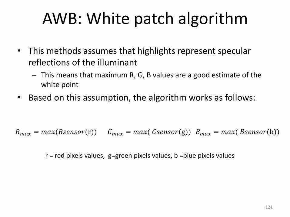
AWB: White patch algorithm
• This methods assumes that highlights represent specular reflections of the illuminant– This means that maximum R, G, B values are a good estimate of the
white point
• Based on this assumption, the algorithm works as follows:
𝑅𝑚𝑎𝑥 = 𝑚𝑎𝑥(𝑅𝑠𝑒𝑛𝑠𝑜𝑟(r))
r = red pixels values, g=green pixels values, b =blue pixels values
𝐺𝑚𝑎𝑥 = 𝑚𝑎𝑥( 𝐺𝑠𝑒𝑛𝑠𝑜𝑟(g)) 𝐵𝑚𝑎𝑥 = 𝑚𝑎𝑥( 𝐵𝑠𝑒𝑛𝑠𝑜𝑟(b))
121
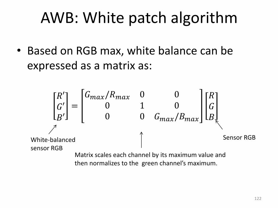
AWB: White patch algorithm
• Based on RGB max, white balance can be expressed as a matrix as:
𝑅′𝐺′𝐵′
=𝐺𝑚𝑎𝑥/𝑅𝑚𝑎𝑥 0 00 1 00 0 𝐺𝑚𝑎𝑥/𝐵𝑚𝑎𝑥
𝑅𝐺𝐵
Sensor RGBWhite-balancedsensor RGB
Matrix scales each channel by its maximum value and then normalizes to the green channel’s maximum.
122
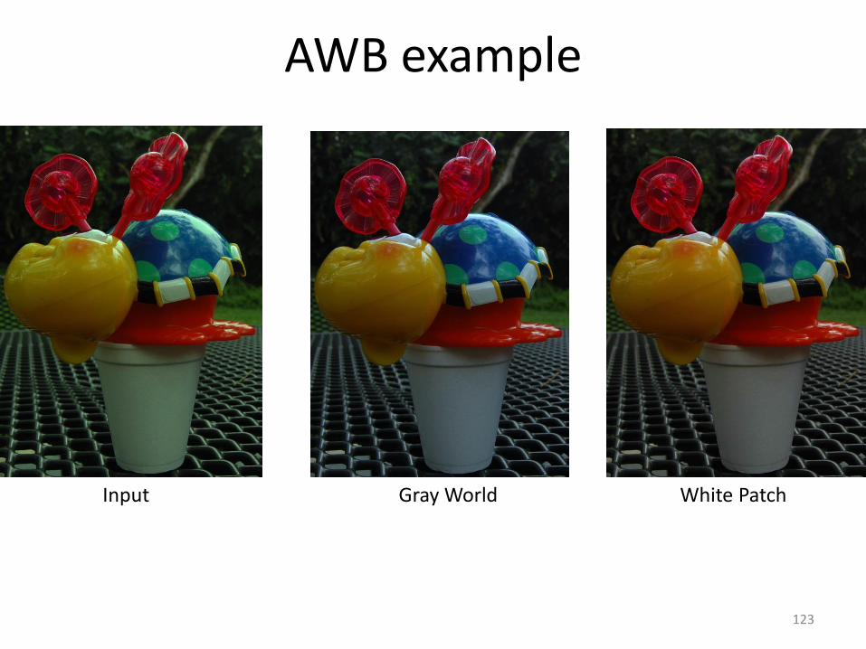
AWB example
White Patch Gray WorldInput
123

Better AWB methods
• Gray world and white patch are very basic algorithms
– These both tend to fail when the image is dominated by large regions of a single color (e.g. a sky image)
• There are many improved versions
• Most improvements focus on how to perform these white point estimation more robustly
• Note: AWB matrix values are often stored in an images Exif file
124
B B B
R R R
RRR
B
B
B
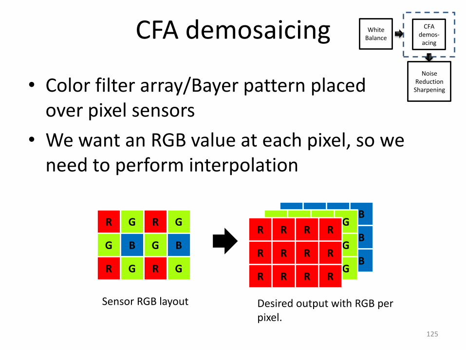
CFA demosaicing
• Color filter array/Bayer pattern placed over pixel sensors
• We want an RGB value at each pixel, so we need to perform interpolation
White Balance
CFAdemos-
acing
Noise Reduction
Sharpening
R G R
G B G
RGR
G
B
G
G G G
R R R
RRR
G
G
G
R R R
R R R
RRR
R
R
R
Sensor RGB layout Desired output with RGB perpixel.
125

Simple interpolation
G2 B3
G6R5
B1
G4
G8 B9B7
R5
G5
B5 ?
?
G2
G6G4
G8
B3B1
B9B7
?
?
B5 = B3B1 B9B7+ + +
4
G5 G4G2 G8G6
4
= + + +
Simply interpolatebased on neighborvalues.
126
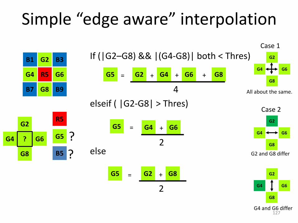
Simple “edge aware” interpolation
G2 B3
G6R5
B1
G4
G8 B9B7
R5
G5
B5 ?
?G2
G6G4
G8
?
If (|G2–G8) && |(G4-G8)| both < Thres)=
elseif ( |G2-G8| > Thres)
else
G4G2 G8G6
4
+ + +
G4 G6
2
+
G2 G8
2
+
G5
G5
G5
=
=
=
G2
G6G4
G8
G2
G6G4
G8
G2
G6G4
G8
Case 1
Case 2
All about the same.
G2 and G8 differ
G4 and G6 differ127

Demosaicing
• These examples are simple algorithms
• Cameras almost certainly use more complex and proprietary algorithms
• Demosaicing can be combined with additional processing
– Highlight clipping
– Sharpening
– Noise reduction
128
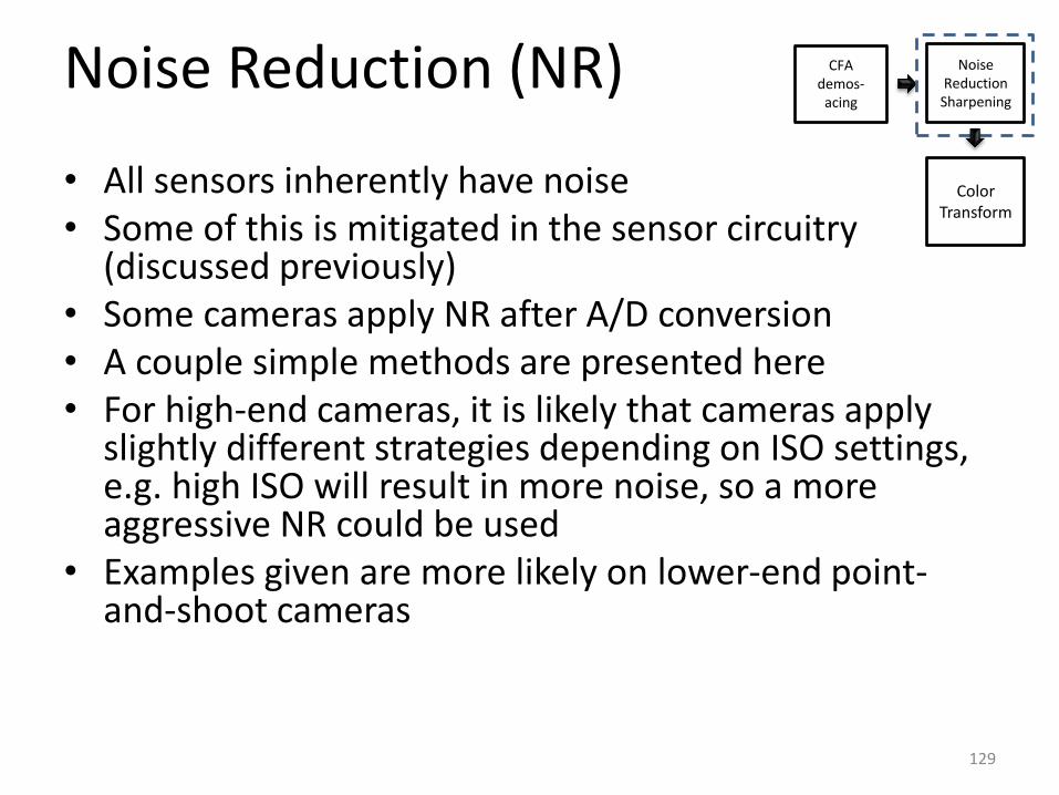
Noise Reduction (NR)
Color Transform
CFAdemos-
acing
Noise Reduction
Sharpening
• All sensors inherently have noise• Some of this is mitigated in the sensor circuitry
(discussed previously) • Some cameras apply NR after A/D conversion • A couple simple methods are presented here• For high-end cameras, it is likely that cameras apply
slightly different strategies depending on ISO settings, e.g. high ISO will result in more noise, so a more aggressive NR could be used
• Examples given are more likely on lower-end point-and-shoot cameras
129
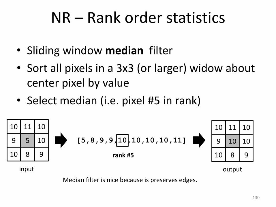
NR – Rank order statistics
• Sliding window median filter
• Sort all pixels in a 3x3 (or larger) widow about center pixel by value
• Select median (i.e. pixel #5 in rank)
10 11 10
9 5 10
10 8 9
input
[5,8,9,9,10,10,10,10,11]
10 11 10
9 10 10
10 8 9
output
rank #5
Median filter is nice because is preserves edges.
130
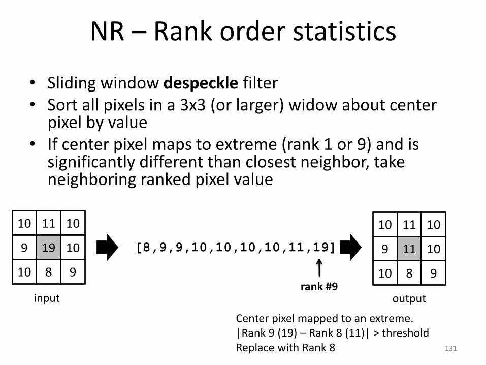
NR – Rank order statistics
• Sliding window despeckle filter• Sort all pixels in a 3x3 (or larger) widow about center
pixel by value• If center pixel maps to extreme (rank 1 or 9) and is
significantly different than closest neighbor, take neighboring ranked pixel value
10 11 10
9 19 10
10 8 9
input
10 11 10
9 11 10
10 8 9
outputrank #9
[8,9,9,10,10,10,10,11,19]
Center pixel mapped to an extreme.|Rank 9 (19) – Rank 8 (11)| > thresholdReplace with Rank 8 131
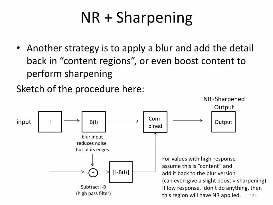
NR + Sharpening
• Another strategy is to apply a blur and add the detail back in “content regions”, or even boost content to perform sharpening
Sketch of the procedure here:
I B(I)input
blur inputreduces noise but blurs edges
|I-B(I)|
Subtract I-B(high pass filter)
Com-bined
For values with high-responseassume this is “content” and add it back to the blur version(can even give a slight boost = sharpening).If low response, don’t do anything, thenthis region will have NR applied.
Output
NR+SharpenedOutput
-
132
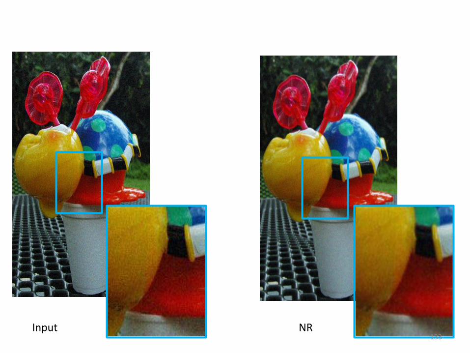
Input NR133
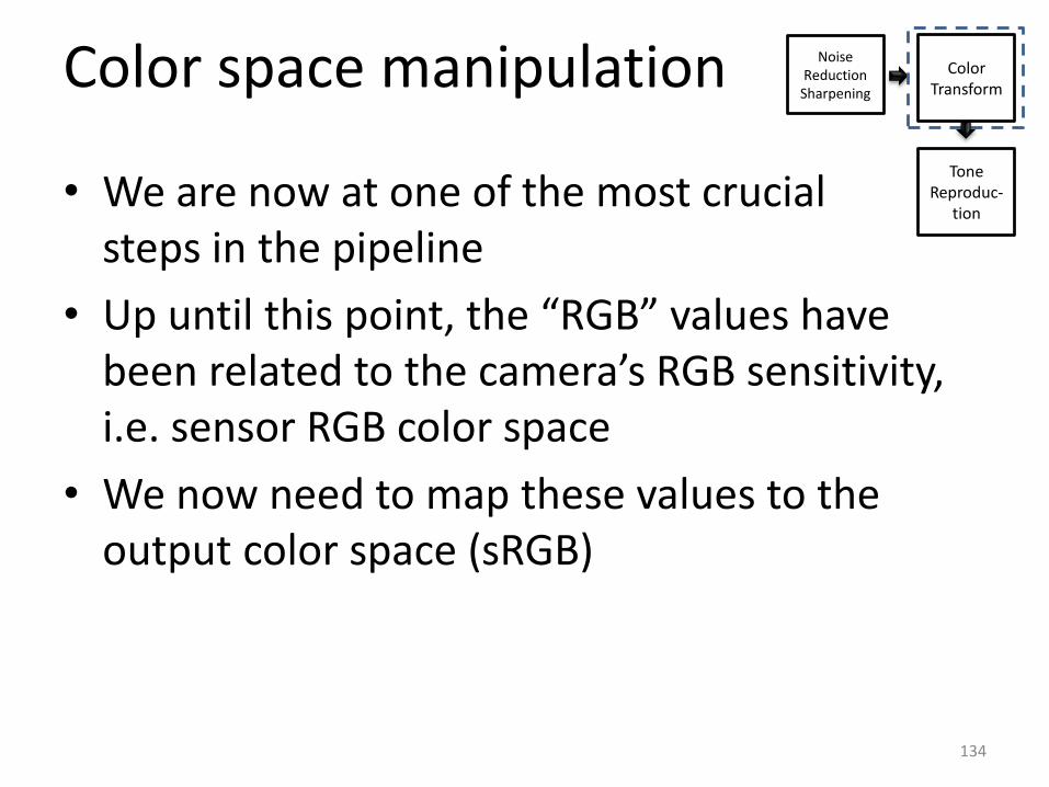
Color space manipulation
• We are now at one of the most crucialsteps in the pipeline
• Up until this point, the “RGB” values have been related to the camera’s RGB sensitivity, i.e. sensor RGB color space
• We now need to map these values to the output color space (sRGB)
ToneReproduc-
tion
Noise Reduction
Sharpening
Color Transform
134
Color space transform
• Color Correction Matrix (CCM)
– Transforms sensor native RGB values into some canonical colorspace (e.g. CIE XYZ) that will eventual be transform to the final sRGB colorspace
• It is important that the white-balance has been performed correctly
135
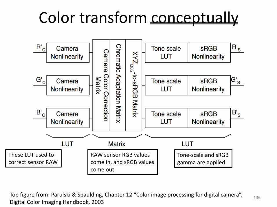
Color transform conceptually
Top figure from: Parulski & Spaulding, Chapter 12 “Color image processing for digital camera”, Digital Color Imaging Handbook, 2003
These LUT used tocorrect sensor RAW
RAW sensor RGB valuescome in, and sRGB valuescome out
Tone-scale and sRGBgamma are applied
136
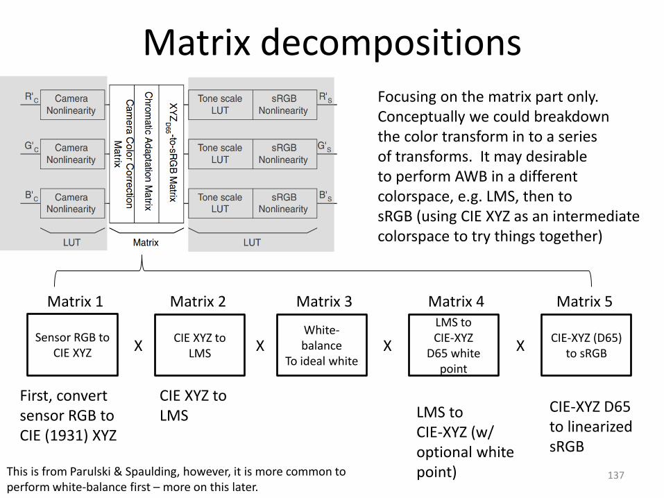
Matrix decompositionsFocusing on the matrix part only.Conceptually we could breakdownthe color transform in to a seriesof transforms. It may desirable to perform AWB in a differentcolorspace, e.g. LMS, then tosRGB (using CIE XYZ as an intermediatecolorspace to try things together)
LMS toCIE-XYZ (w/optional whitepoint)
Sensor RGB to CIE XYZ
Matrix 1
CIE XYZ to LMS
White-balance
To ideal white
LMS to CIE-XYZ
D65 white point
CIE-XYZ (D65) to sRGB
Matrix 2 Matrix 3 Matrix 4 Matrix 5
X X X X
First, convertsensor RGB toCIE (1931) XYZ
CIE XYZ to LMS
CIE-XYZ D65to linearizedsRGB
137This is from Parulski & Spaulding, however, it is more common to perform white-balance first – more on this later.

Tone-mapping
• Non-linear mapping of RGB tones
• Applied to achieve some preferred tone-reproduction – This is not sRGB gamma
– This is to make the images look nice
• To some degree this mimics the nonlinearity in film (known as the Hurter-Driffield Curves)
• Each camera has its own unique tone-mapping (possibly multiple ones)
JPEGCompress
-ion
Color Transform
ToneReproduc-
tion
138

Examples
From Grossberg & Nayar (CVPR’03)
(RAW or linearize sRGB)
Here are several examples of tone-mappings for a white range of cameras.The x-axis is the input “RAW” (or linearized-sRGB), the y-axis is the outputAfter tone mapping.
139

Tone-mapped examples
Input
140

Note about tone-mapping
• It is worth noting, that up until this stage, our color values (either RAW or linear sRGB) are related to incoming light in a linear fashion
• After this step, that relationship is broken
• Unlike the sRGB gamma (which is known), the tone-mapping is propriety and can only be found by a calibration procedure
141

JPEG compression
• Joint Photographic Experts Group (JPEG)
• Lossy compression strategy based on the 2D Discrete Cosine Transformation (DCT)
• The by far the most widely adopted standard for image storage
Exif metadata
ToneReproduc-
tion
JPEGCompress
-ion
142

JPEG approach
Take original image and
Break it into 8x8 blocks
8x8 DCT(Forward DCT)
on each block
Quantize DCT coefficients
via
Quantization “Table”
C’(u,v) = round(C(u,v)/T(u,v))
“Zig-zag” Order Coefficients
RLE
AC Vector
0Differential
coding DC component
Huffman
EncodeJPEG bitstream
T(u,v)
f(x,y) - 128
(normalize between –128 to 127)
JPEG applies almost every compression trick known.
1) Transform coding, 2) psychovisual (loss), 3) Run-length-encoding (RLE), 4) Difference coding, and Huffman.143

JPEG quality
• The amount of quantization applied on the DCT coefficients amounts to a “quality” factor– More quantization = better compression (smaller file size)
– More quantization = lower quality
• Cameras generally allow a range that you can select
Image from nphotomag.com 144

Exif metadata
• Exchangeable image file format (Exif)
• Created by the Japan Electronics and Information Technology Industries Association (JEITA)
• Associates meta data with images
– Date/time
– Camera settings (basic)• Image size, aperture, shutter speed, focal length, ISO speed, metering
mode (how exposure was estimated)
– Additional info (from in some Exif files)• White-balance settings, even matrix coefficients of white-balnace
• Picture style (e.g. landscape, vivid, standard, portrait)
• Output color space (e.g. sRGB, Adobe RGB, RAW)
• GPS info
• More . . .
Save to flash
memory
JPEGCompress
-ion
Exif metadata
145
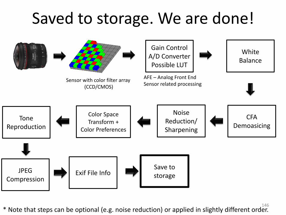
Saved to storage. We are done!
Gain ControlA/D ConverterPossible LUT
AFE – Analog Front EndSensor related processing
Sensor with color filter array (CCD/CMOS)
CFADemoasicing
White Balance
Color Space Transform +
Color Preferences
Tone Reproduction
JPEG Compression
Exif File Info
Noise Reduction/Sharpening
Save to storage
* Note that steps can be optional (e.g. noise reduction) or applied in slightly different order.146
Pipeline comments
• Again, important to stress that the exact steps mentioned in these notes only serve as a guide of common steps that take place
• For different camera makes/models, these could be performed in different order (e.g. white-balance after demosaicing) and in different ways (e.g. combining sharpening with demosaicing)
147
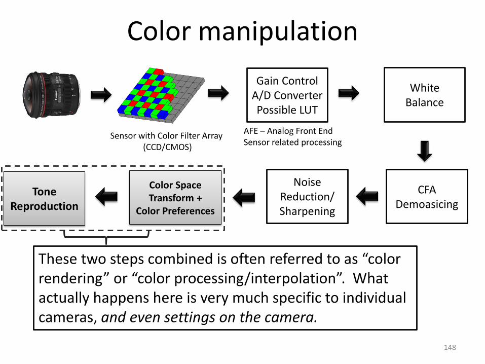
Color manipulation
Gain ControlA/D ConverterPossible LUT
AFE – Analog Front EndSensor related processing
Sensor with Color Filter Array (CCD/CMOS)
CFADemoasicing
White Balance
Noise Reduction/Sharpening
These two steps combined is often referred to as “color rendering” or “color processing/interpolation”. What actually happens here is very much specific to individualcameras, and even settings on the camera.
Color Space Transform +
Color Preferences
Tone Reproduction
148

ICC and color profiles
• International Color Consortium (ICC)– In charge of developing several ISO standards for color
management
• Promote the use of ICC profiles
• ICC profiles are intended for device manufacturers to describe how their respective color spaces (e.g. sensor RGB) map to canonical color spaces called Profile Connection Spaces (PCS)
• PCS are similar to linking all devices to CIE XYZ, but are more flexible allowing for additional spaces to be defined (beyond CIE XYZ)
149
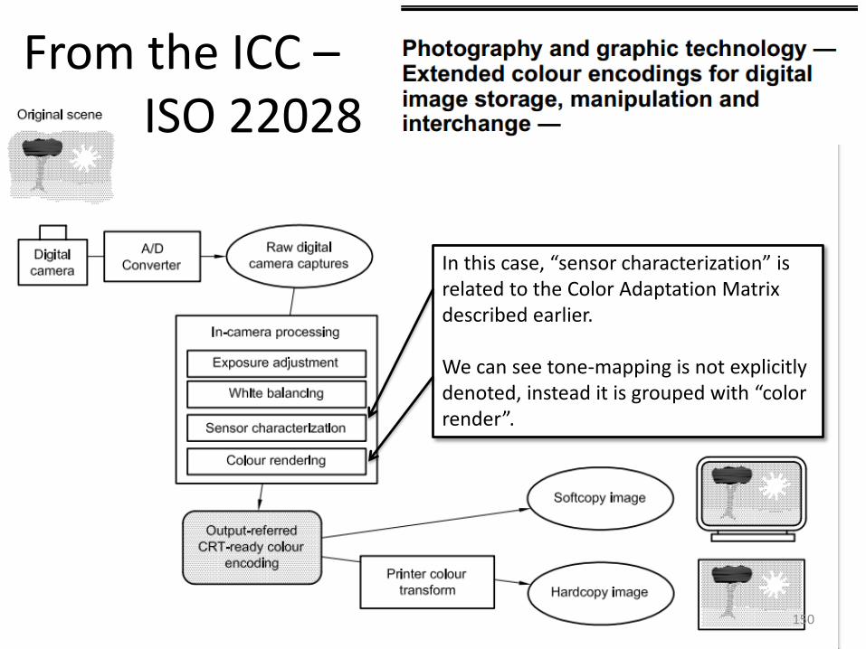
From the ICC –ISO 22028
In this case, “sensor characterization” isrelated to the Color Adaptation Matrix described earlier.
We can see tone-mapping is not explicitlydenoted, instead it is grouped with “color render”.
150
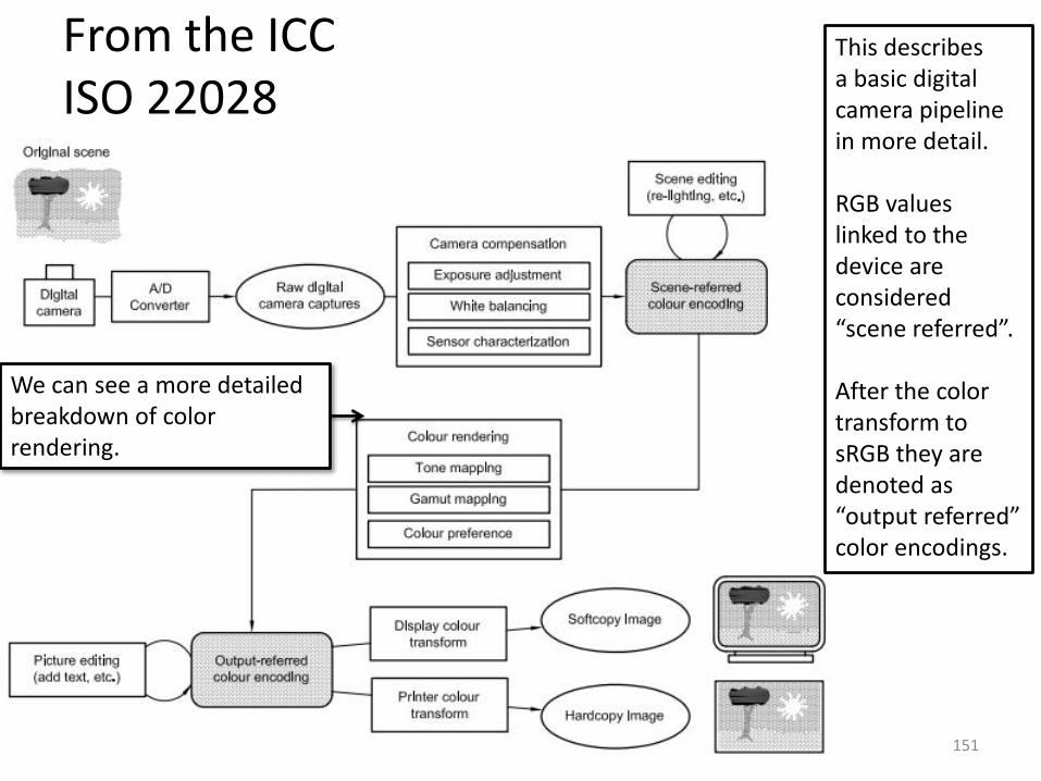
From the ICC ISO 22028
This describesa basic digitalcamera pipeline in more detail.
RGB valueslinked to the device areconsidered “scene referred”.
After the colortransform to sRGB they aredenoted as“output referred”color encodings.
We can see a more detailed breakdown of color rendering.
151
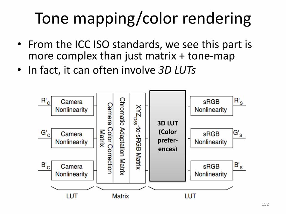
Tone mapping/color rendering
• From the ICC ISO standards, we see this part is more complex than just matrix + tone-map
• In fact, it can often involve 3D LUTs
3D LUT(Color prefer-ences)
152

Camera image processors
• Steps applied after the sensor output are generally performed by an “image processor” on the camera
• Different cameras use different processing boards/software
• High-end cameras and associated processors – Nikon – Expeed
– Fuji – Real photo engine
– Canon – DIGIC
– Sony – BIONZ
– . . .
• Mobile-devices– Qualcomm - Snapdragon
– Nvidia - Tegra
153
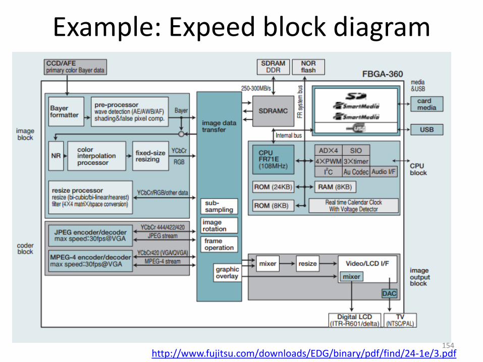
Example: Expeed block diagram
http://www.fujitsu.com/downloads/EDG/binary/pdf/find/24-1e/3.pdf154
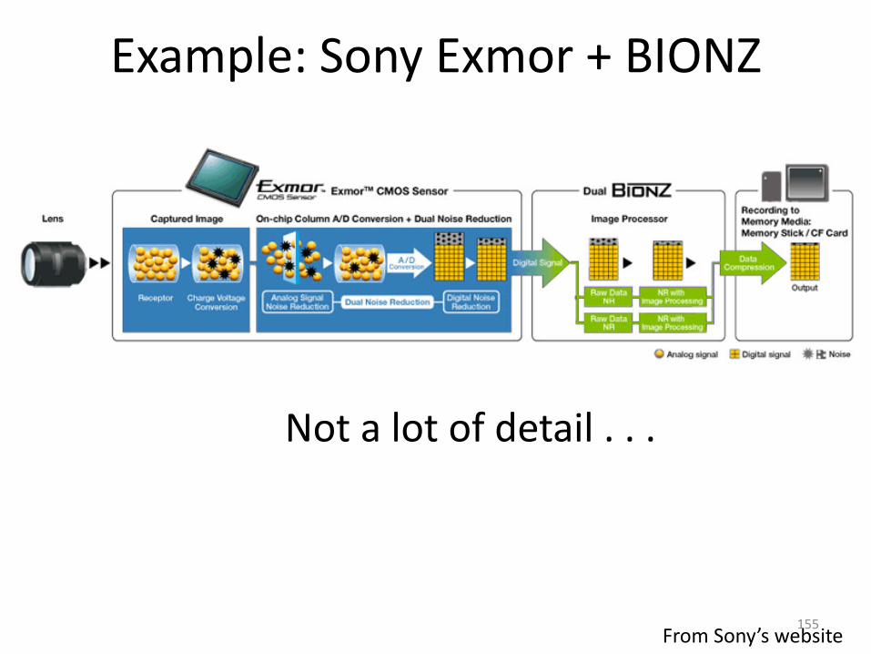
Example: Sony Exmor + BIONZ
Not a lot of detail . . .
From Sony’s website 155

Tutorial schedule
• Part 1 (General Part)
– Motivation
– Review of color/color spaces
– Overview of camera imaging pipeline
• Part 2* (Specific Part)
– Modeling the in-camera color pipeline
– Photo-refinishing
• Part 3 (Wrap Up)
– The good, the bad, and the ugly of commodity cameras and computer vision research
– Concluding Remarks
156* Mainly involves shameless self-promotion of my group’s work.

Part 2: Modeling the onboard
camera color processing pipeline

Part 2 Acknowledgements
Dr. Hai-ting Lin (NUS/U. Delaware)
Prof. Sabine Süsstrunk(EPFL)
Steven Lin(MSR-Asia)
Dr. Zheng Lu(NUS/City U Hong Kong)
Dr. Steven Lin(MSR-Asia)
158
Prof. Seon Joo Kim (Yonsei)
S. J. Kim et al “A New In-Camera Imaging Model for Color Computer Vision and its Application”, IEEE Transactions on Pattern Analysis and Machine Intelligence, Dec 2012

Standard color spaces are great
CamerasRGB Image
sRGB -> CIE XYZ -> Display (ICC Profile)
“The real scene”
?
159
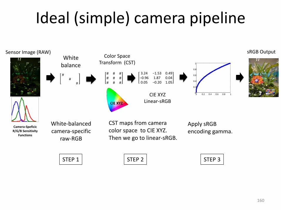
Ideal (simple) camera pipeline
Sensor Image (RAW)
Camera-SpeficicR/G/B Sensitivity
Functions
Whitebalance
STEP 1
White-balancedcamera-specific
raw-RGB
Color Space Transform (CST)
CIE XYZ
CIE XYZLinear-sRGB
3.24 −1.53 0.49−0.96 1.87 0.040.05 −0.20 1.05
STEP 2
CST maps from camera color space to CIE XYZ. Then we go to linear-sRGB.
STEP 3
0 0.2 0.4 0.6 0.8 10
0.2
0.4
0.6
0.8
1
Apply sRGBencoding gamma.
sRGB Output
160

161
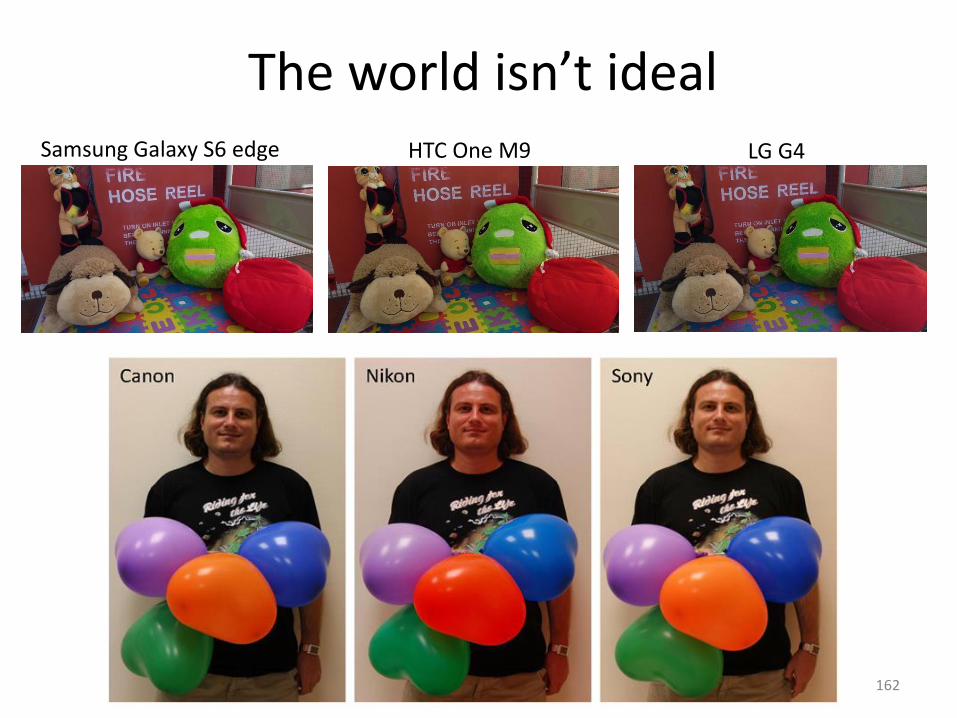
The world isn’t idealSamsung Galaxy S6 edge HTC One M9 LG G4
162
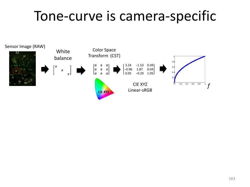
Tone-curve is camera-specific
Sensor Image (RAW)White
balance
Color Space Transform (CST)
CIE XYZ
CIE XYZLinear-sRGB
3.24 −1.53 0.49−0.96 1.87 0.040.05 −0.20 1.05
0 0.2 0.4 0.6 0.8 10
0.2
0.4
0.6
0.8
1
f
163
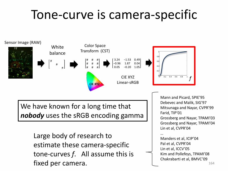
Tone-curve is camera-specific
Sensor Image (RAW)White
balance
Color Space Transform (CST)
CIE XYZ
CIE XYZLinear-sRGB
3.24 −1.53 0.49−0.96 1.87 0.040.05 −0.20 1.05
0 0.2 0.4 0.6 0.8 10
0.2
0.4
0.6
0.8
1
We have known for a long time that nobody uses the sRGB encoding gamma
Mann and Picard, SPIE’95Debevec and Malik, SIG’97Mitsunaga and Nayar, CVPR’99Farid, TIP’01Grossberg and Nayar, TPAMI’03Grossberg and Nayar, TPAMI’04Lin et al, CVPR’04…Manders et al, ICIP’04Pal et al, CVPR’04Lin et al, ICCV’05Kim and Pollefeys, TPAMI’08Chakrabarti et al, BMVC’09
Large body of research to estimate these camera-specifictone-curves f. All assume this is fixed per camera.
f
164

Manufacturers give us a hint
From Canon’s user manual
165

Nikon D7000 - RAW
166

NEUTRAL
167
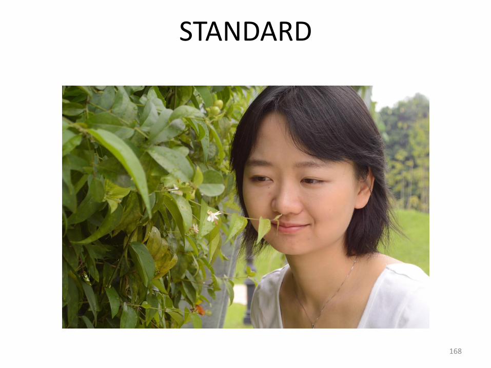
STANDARD
168
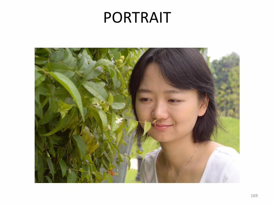
PORTRAIT
169
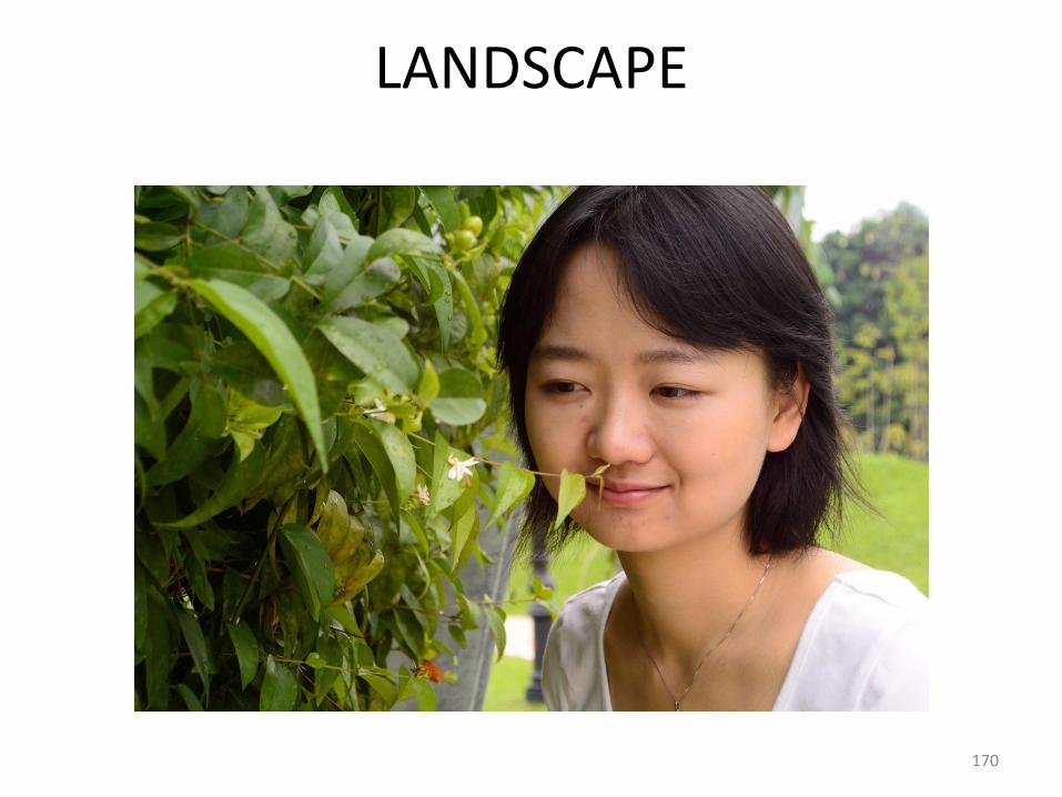
LANDSCAPE
170
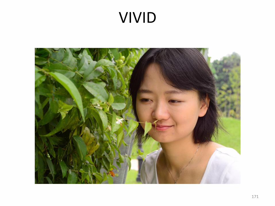
VIVID
171

Camera = light-measuring device
“All models are wrong, but some are useful; how wrong can they be and still be useful.”
George BoxProfessor Emeritus of Statistics U. Wisconsin
172
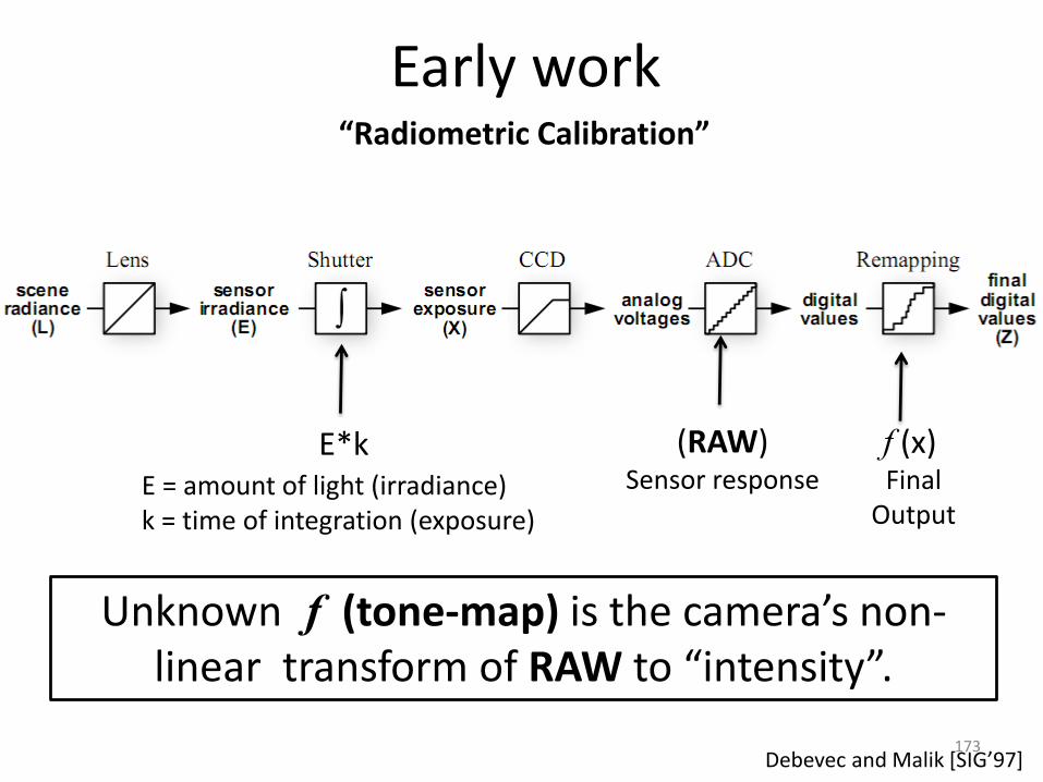
Early work
Debevec and Malik [SIG’97]
f (x) Final
Output
(RAW)Sensor response
Unknown f (tone-map) is the camera’s non-linear transform of RAW to “intensity”.
“Radiometric Calibration”
E*kE = amount of light (irradiance)k = time of integration (exposure)
173

Accepted model
bx
gx
rx
E
E
E
bx
gx
rx
E
E
E
T
bx
gx
rx
e
e
e
=
)(
)(
)(
bxb
gxg
rxr
ef
ef
ef
bx
gx
rx
i
i
i
=
(RAW) T is a 3x3 matrix i is the sRGB output and f is a non-linear function
(small e are white-balancedRAW)
174
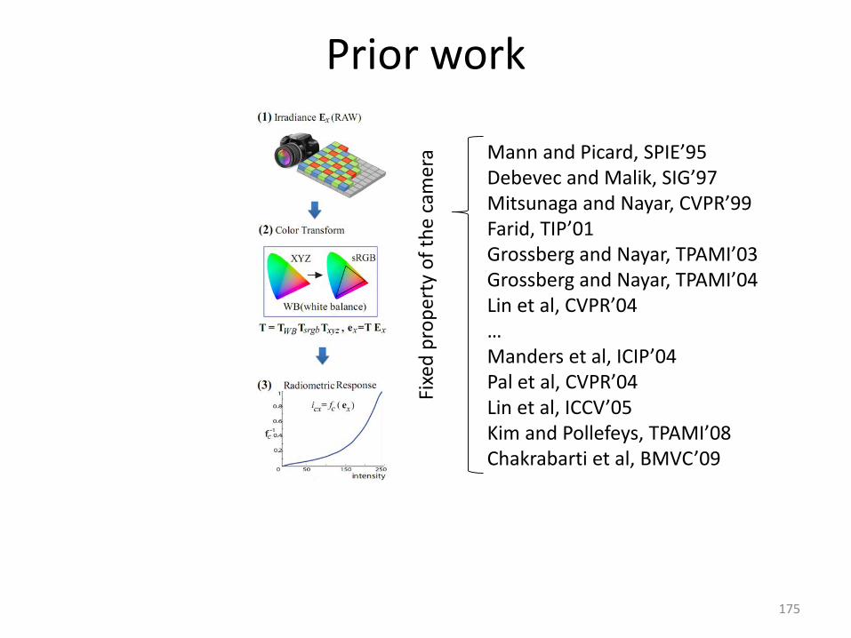
Prior work
Mann and Picard, SPIE’95Debevec and Malik, SIG’97Mitsunaga and Nayar, CVPR’99Farid, TIP’01Grossberg and Nayar, TPAMI’03Grossberg and Nayar, TPAMI’04Lin et al, CVPR’04…Manders et al, ICIP’04Pal et al, CVPR’04Lin et al, ICCV’05Kim and Pollefeys, TPAMI’08Chakrabarti et al, BMVC’09
Fixe
d p
rop
erty
of
the
cam
era
175
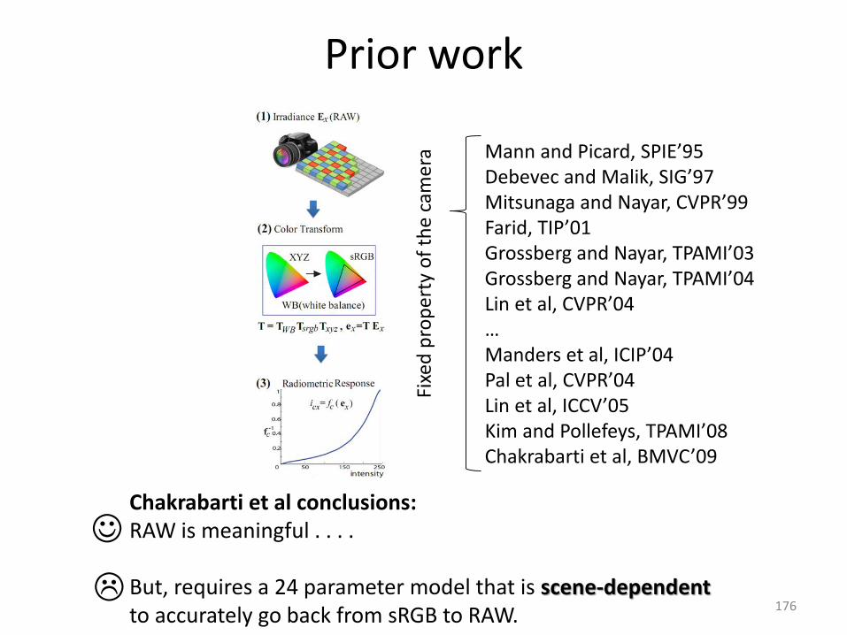
Prior work
Mann and Picard, SPIE’95Debevec and Malik, SIG’97Mitsunaga and Nayar, CVPR’99Farid, TIP’01Grossberg and Nayar, TPAMI’03Grossberg and Nayar, TPAMI’04Lin et al, CVPR’04…Manders et al, ICIP’04Pal et al, CVPR’04Lin et al, ICCV’05Kim and Pollefeys, TPAMI’08Chakrabarti et al, BMVC’09
Chakrabarti et al conclusions:RAW is meaningful . . . .
But, requires a 24 parameter model that is scene-dependentto accurately go back from sRGB to RAW.
Fixe
d p
rop
erty
of
the
cam
era
176
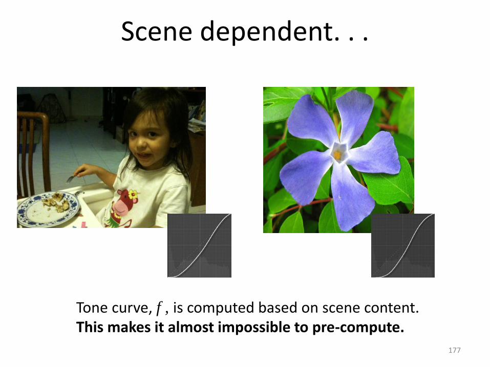
Scene dependent. . .
Tone curve, f , is computed based on scene content. This makes it almost impossible to pre-compute.
177
bx
gx
rx
E
E
E
T
bx
gx
rx
e
e
e
=
)(
)(
)(
bx
gxg
rxr
ef
ef
ef
bx
gx
rx
i
i
i
=
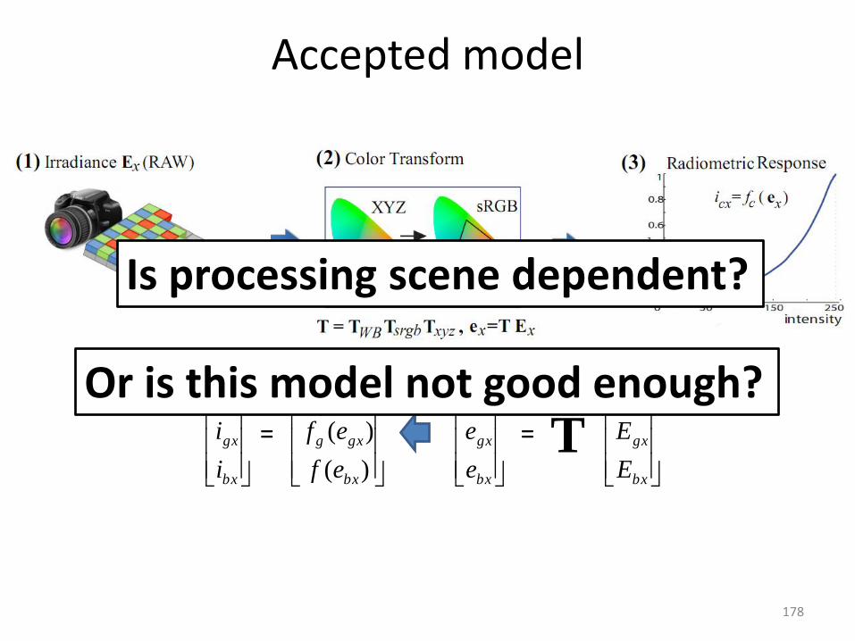
Accepted model
Or is this model not good enough?
Is processing scene dependent?
178

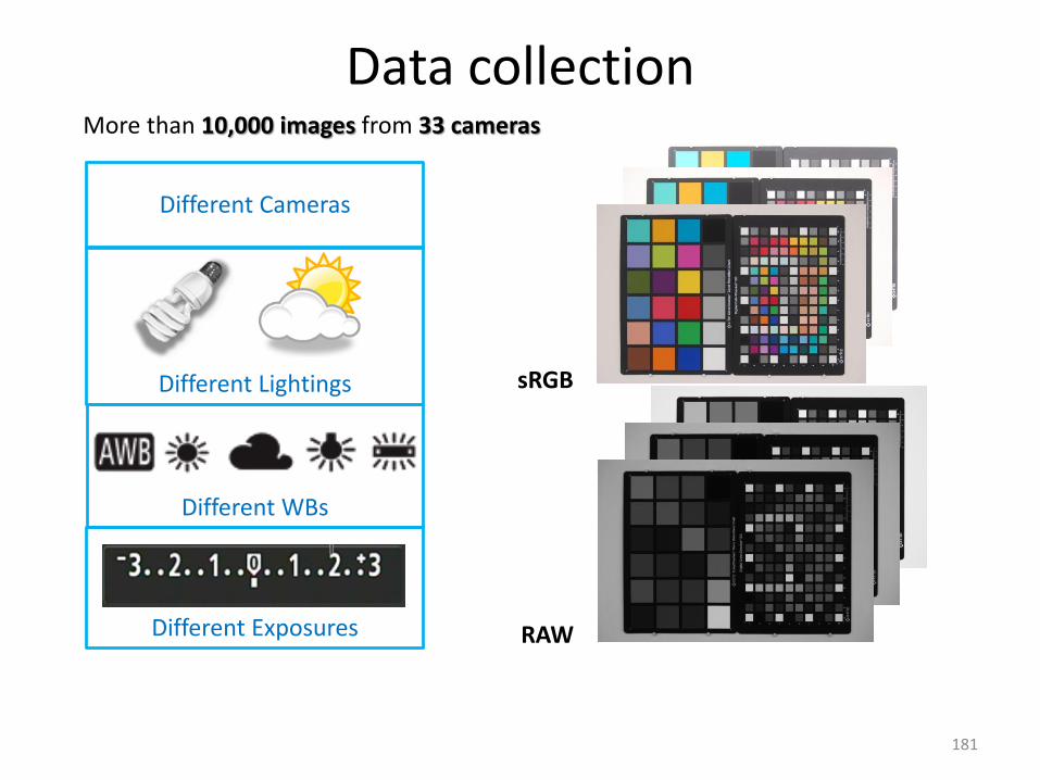
Our experiment: data collection
• More than 10,000 images from 33 cameras from DSLRs to point-and-shoots
• Images of color charts under indoor / outdoor (cloudy)
• Images are taken at all possible shutter speeds, at multiple aperture, and white balance settings. JPEG / RAW both captured if possible.
* Special shooting features such as lighting optimizer are turned off
179Lin et al, ICCV 2011; Kim et al, TPAMI 2012

Different Lightings
Different Cameras
Different WBs
Different Exposures
More than 10,000 images from 33 cameras
sRGB
RAW
Data collection
180
Different Lightings
Different Cameras
Different WBs
Different Exposures
More than 10,000 images from 33 cameras
sRGB
RAW
Data collection
181
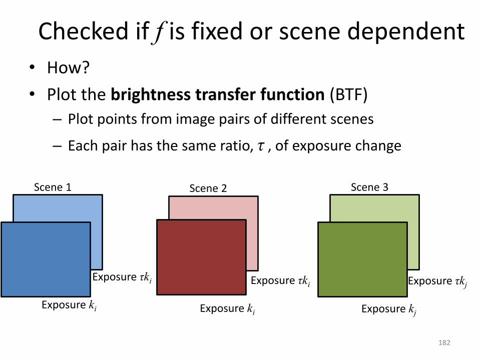
Checked if f is fixed or scene dependent
• How?
• Plot the brightness transfer function (BTF)
– Plot points from image pairs of different scenes
– Each pair has the same ratio, τ , of exposure change
Scene 1
Exposure ki
Exposure τki
Scene 2 Scene 3
Exposure ki
Exposure τki
Exposure kj
Exposure τkj
182
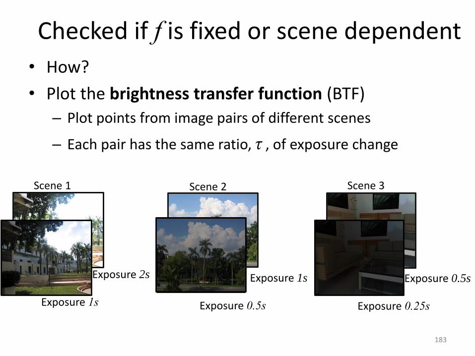
Checked if f is fixed or scene dependent
• How?
• Plot the brightness transfer function (BTF)
– Plot points from image pairs of different scenes
– Each pair has the same ratio, τ , of exposure change
Scene 1
Exposure 1s
Exposure 2s
Scene 2 Scene 3
Exposure 0.5s
Exposure 1s
Exposure 0.25s
Exposure 0.5s
183

Checked if f is fixed or scene dependent
• How?
• Plot the brightness transfer function (BTF)
– Plot points from image pairs of different scenes
– Each pair has the same ratio, τ , of exposure change
Scene 1
Exposure 1s
Exposure 2s
Scene 2 Scene 3
Exposure 0.5s
Exposure 1s
Exposure 0.25s
Exposure 0.5s
184
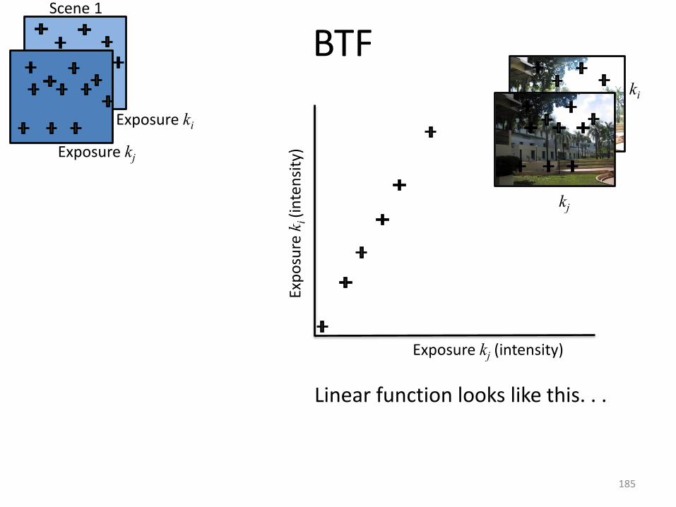
BTFScene 1
Exposure kj
Exposure ki
Exposure kj (intensity)
Exp
osu
re ki(i
nte
nsi
ty)
Linear function looks like this. . .
kj
ki
185
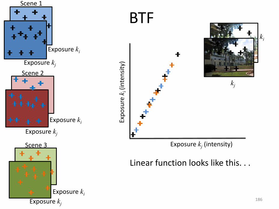
BTFScene 1
Exposure kj
Exposure ki
Linear function looks like this. . .
Scene 2
Exposure kj
Exposure ki
Scene 3
Exposure kj
Exposure ki
Exposure kj (intensity)
Exp
osu
re ki(i
nte
nsi
ty)
kj
ki
186
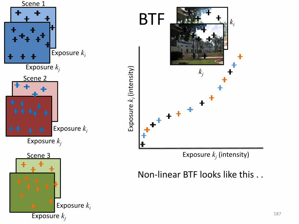
BTFScene 1
Exposure kj
Exposure ki
Non-linear BTF looks like this . .
Scene 2
Exposure kj
Exposure ki
Scene 3
Exposure kj
Exposure ki
Exposure kj (intensity)
Exp
osu
re ki(i
nte
nsi
ty)
kj
ki
187
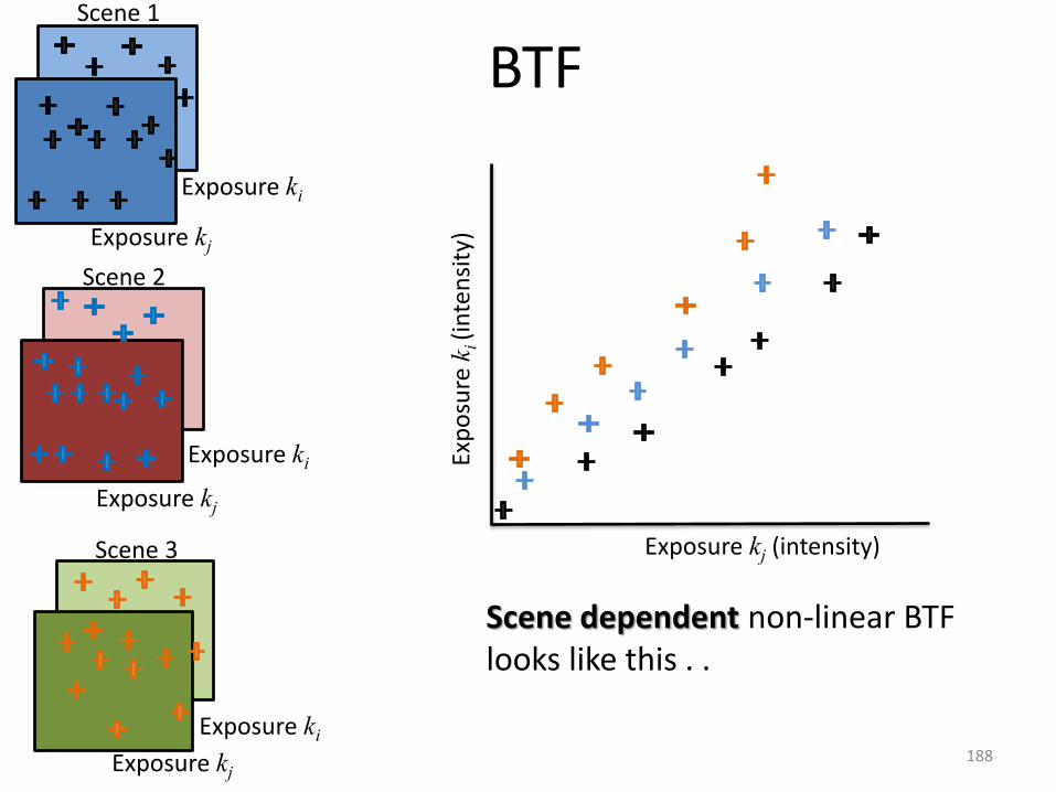
BTFScene 1
Exposure kj
Exposure ki
Scene dependent non-linear BTF looks like this . .
Scene 2
Exposure kj
Exposure ki
Scene 3
Exposure kj
Exposure ki
Exposure kj (intensity)
Exp
osu
re ki(i
nte
nsi
ty)
188

For the most part . . . it was ok
189
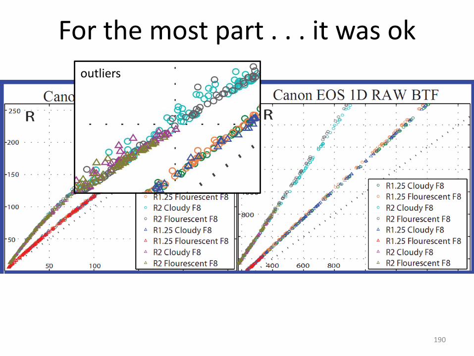
For the most part . . . it was ok
outliers
190

Outliers were not scene dependent.
Outliers were color dependent.
Where are the outliners?
191
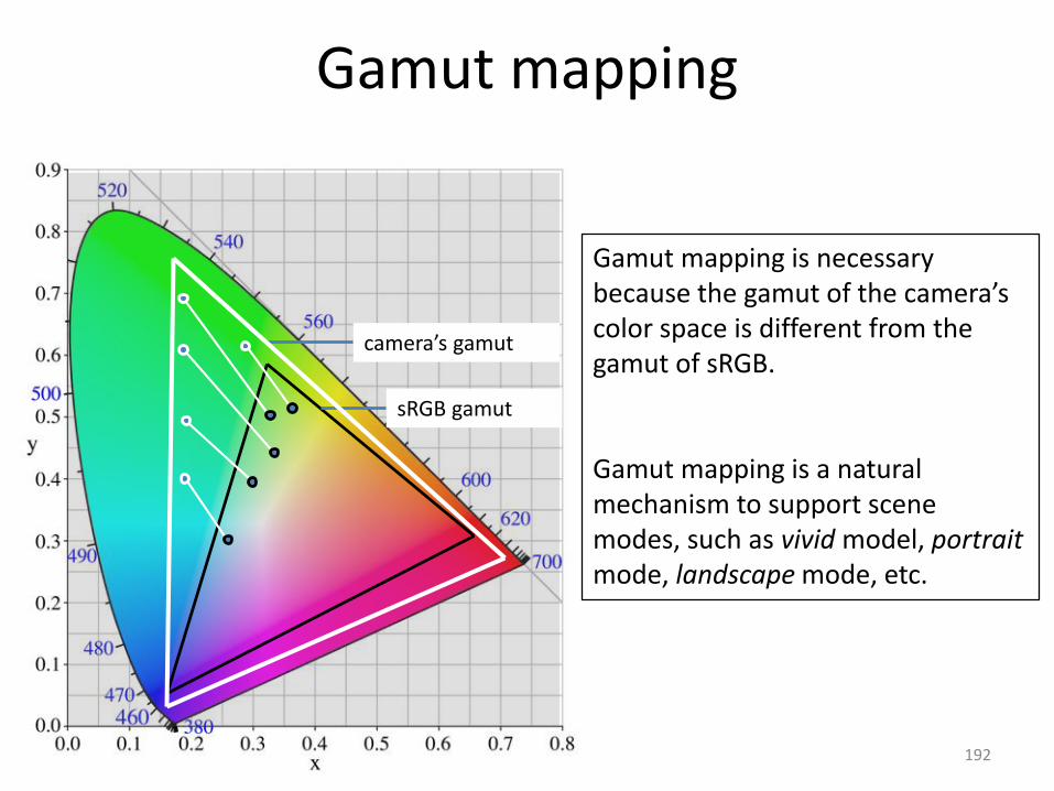
sRGB gamut
camera’s gamut
Gamut mapping is necessary because the gamut of the camera’s color space is different from the gamut of sRGB.
Gamut mapping is a natural mechanism to support scene modes, such as vivid model, portraitmode, landscape mode, etc.
Gamut mapping
192

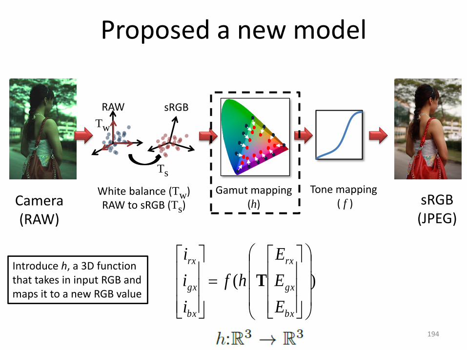
Proposed a new model
Gamut mapping (h)
Tone mapping( f )
RAW
Tw
sRGB
Ts
RAW to sRGB (Ts)White balance (Tw)
sRGB(JPEG)
Camera(RAW)
193
)(
bx
gx
rx
bx
gx
rx
E
E
E
hf
i
i
i
T
Gamut mapping (h)
Tone mapping( f )
RAW
Tw
sRGB
Ts
RAW to sRGB (Ts)White balance (Tw)
sRGB(JPEG)
Camera(RAW)
Proposed a new model
Introduce h, a 3D functionthat takes in input RGB andmaps it to a new RGB value
194
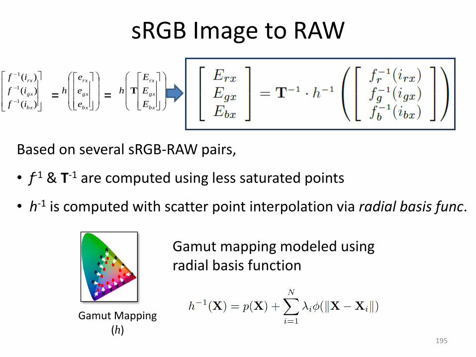
sRGB Image to RAW
Based on several sRGB-RAW pairs,
• f-1 & T-1 are computed using less saturated points
• h-1 is computed with scatter point interpolation via radial basis func.
bx
gx
rx
e
e
e
h
)(
)(
)(
1
1
1
bx
gx
rx
if
if
if
=
bx
gx
rx
E
E
E
h T=
Gamut Mapping (h)
Gamut mapping modeled using radial basis function
195

RAW
sRGB(JPEG)
RAW to sRGB (Ts)
Gamut mapping (h)
Tone mapping( f )
sRGB
Tw
Ts
White balance (Tw)Camera(RAW)
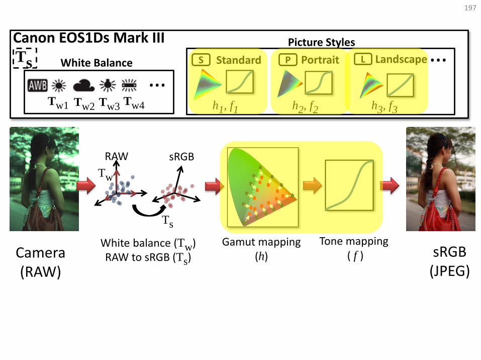
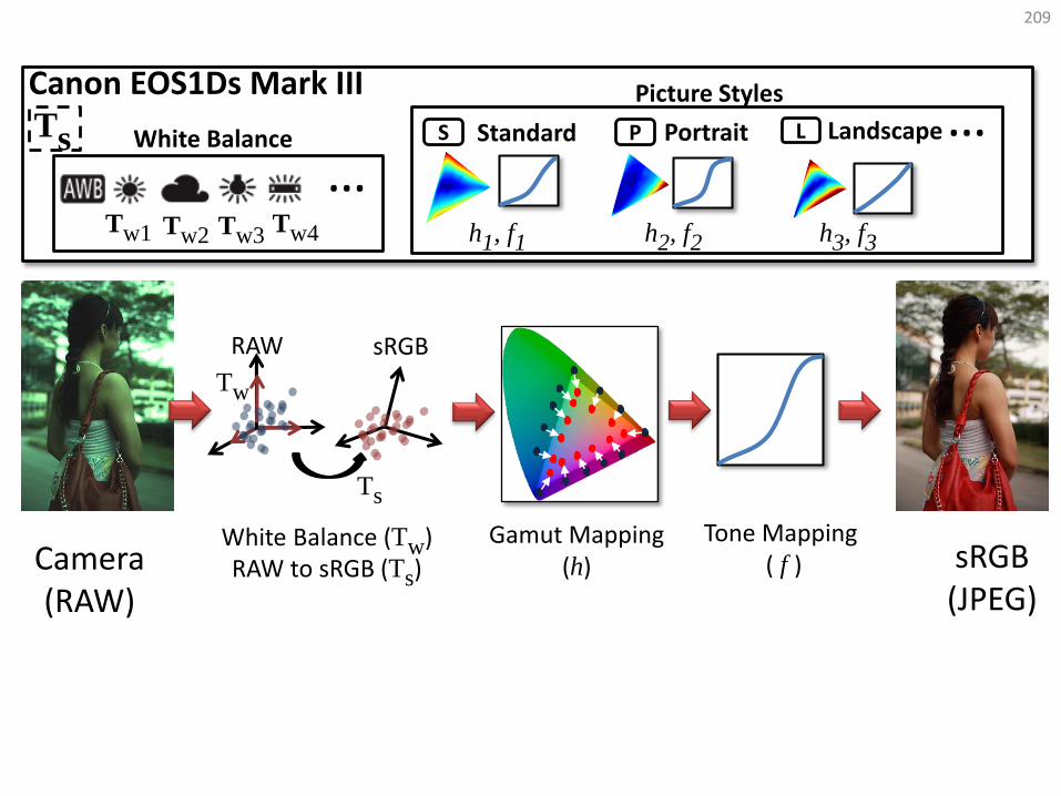
Canon EOS1Ds Mark III
……Ts
Tw1
White Balance
Picture Styles
h1, f1Tw2 Tw3
Tw4 h2, f2 h3, f3
Standard Portrait LandscapeS P L
196
RAW
sRGB(JPEG)
RAW to sRGB (Ts)
Gamut mapping (h)
Tone mapping( f )
sRGB
Canon EOS1Ds Mark III
……Ts
Tw1
White Balance
Picture Styles
h1, f1Tw2 Tw3
Tw4 h2, f2 h3, f3
Tw
Ts
White balance (Tw)Camera(RAW)
Standard Portrait LandscapeS P L
197
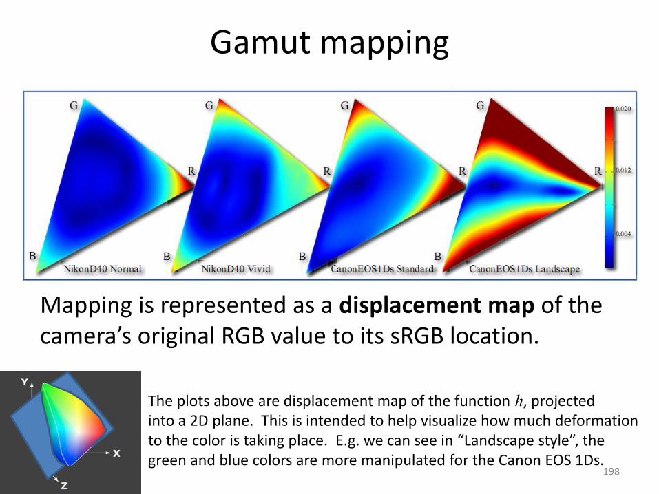
Gamut mapping
Mapping is represented as a displacement map of the camera’s original RGB value to its sRGB location.
198
The plots above are displacement map of the function h, projectedinto a 2D plane. This is intended to help visualize how much deformationto the color is taking place. E.g. we can see in “Landscape style”, the green and blue colors are more manipulated for the Canon EOS 1Ds.

Experiments : Mapping sRGB back to RAW
Canon EOS1D
input sRGB image ground truth RAW
199
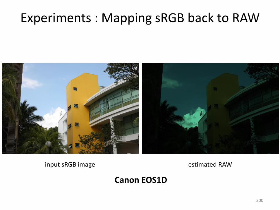
Canon EOS1D
input sRGB image estimated RAW
Experiments : Mapping sRGB back to RAW
200
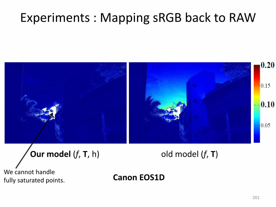
Canon EOS1D
Our model (f, T, h) old model (f, T)
We cannot handlefully saturated points.
Experiments : Mapping sRGB back to RAW
201

Canon EOS550D
input sRGB image ground truth RAW
Experiments : Mapping sRGB back to RAW
202
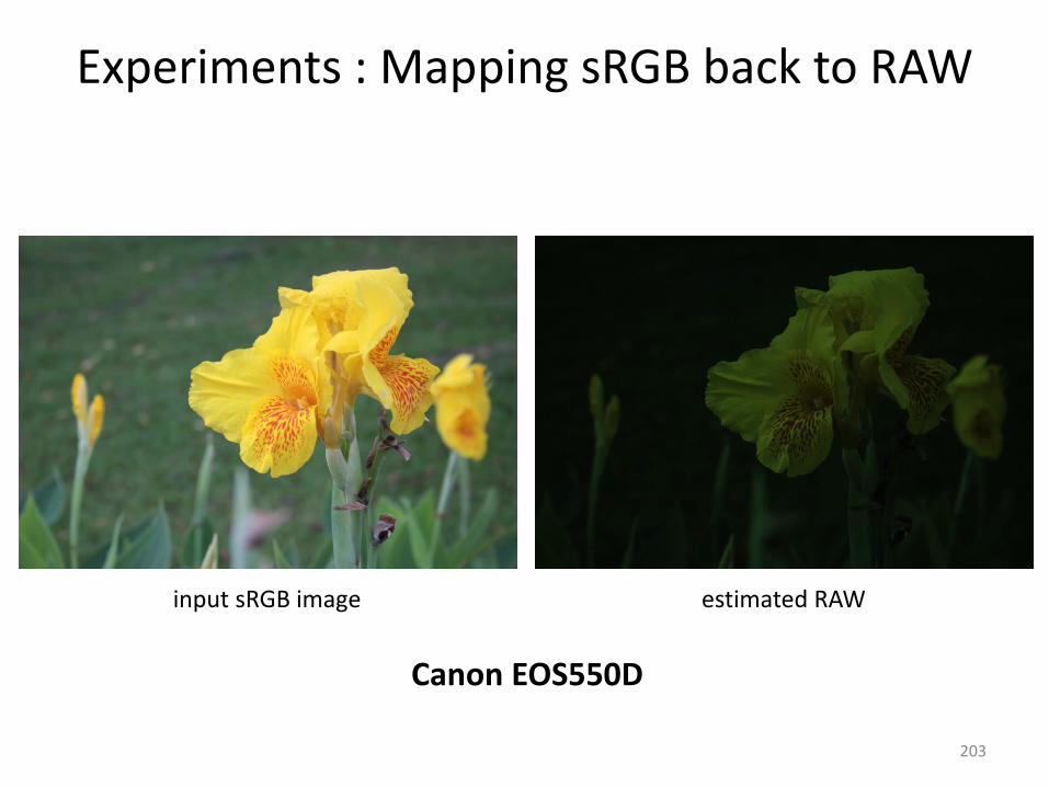
Canon EOS550D
input sRGB image estimated RAW
Experiments : Mapping sRGB back to RAW
203
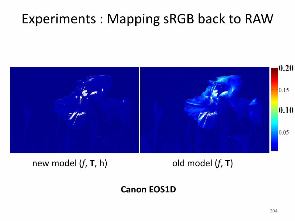
Canon EOS1D
new model (f, T, h) old model (f, T)
Experiments : Mapping sRGB back to RAW
204

Sony A200
input sRGB image ground truth RAW
Experiments : Mapping sRGB back to RAW
205
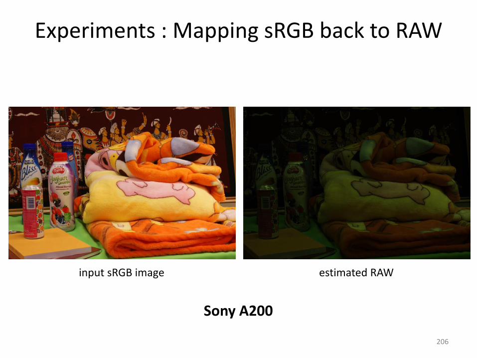
Sony A200
input sRGB image estimated RAW
Experiments : Mapping sRGB back to RAW
206
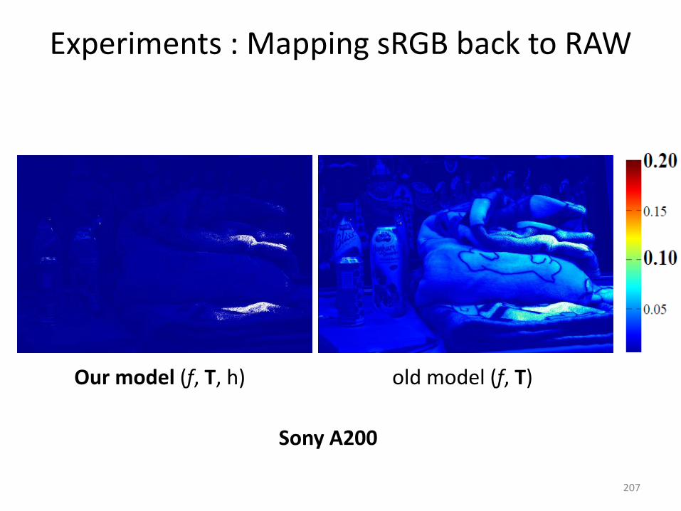
Sony A200
Our model (f, T, h) old model (f, T)
Experiments : Mapping sRGB back to RAW
207

Application: Photo Refinishing
208
RAW
sRGB(JPEG)
RAW to sRGB (Ts)
Gamut Mapping (h)
Tone Mapping( f )
sRGB
Tw
Ts
White Balance (Tw)Camera(RAW)
Canon EOS1Ds Mark III
……Ts
Tw1
White Balance
Picture Styles
h1, f1Tw2 Tw3
Tw4 h2, f2 h3, f3
Standard Portrait LandscapeS P L
209
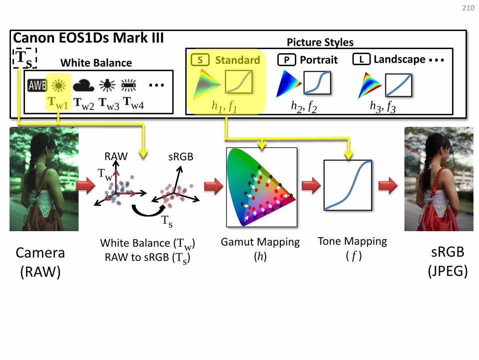
Canon EOS1Ds Mark III
……Ts
Tw1
White Balance
Picture Styles
h1, f1Tw2 Tw3
Tw4 h2, f2 h3, f3
RAW
sRGB(JPEG)
RAW to sRGB (Ts)
Gamut Mapping (h)
Tone Mapping( f )
sRGB
Tw
Ts
White Balance (Tw)Camera(RAW)
Standard Portrait LandscapeS P L
210
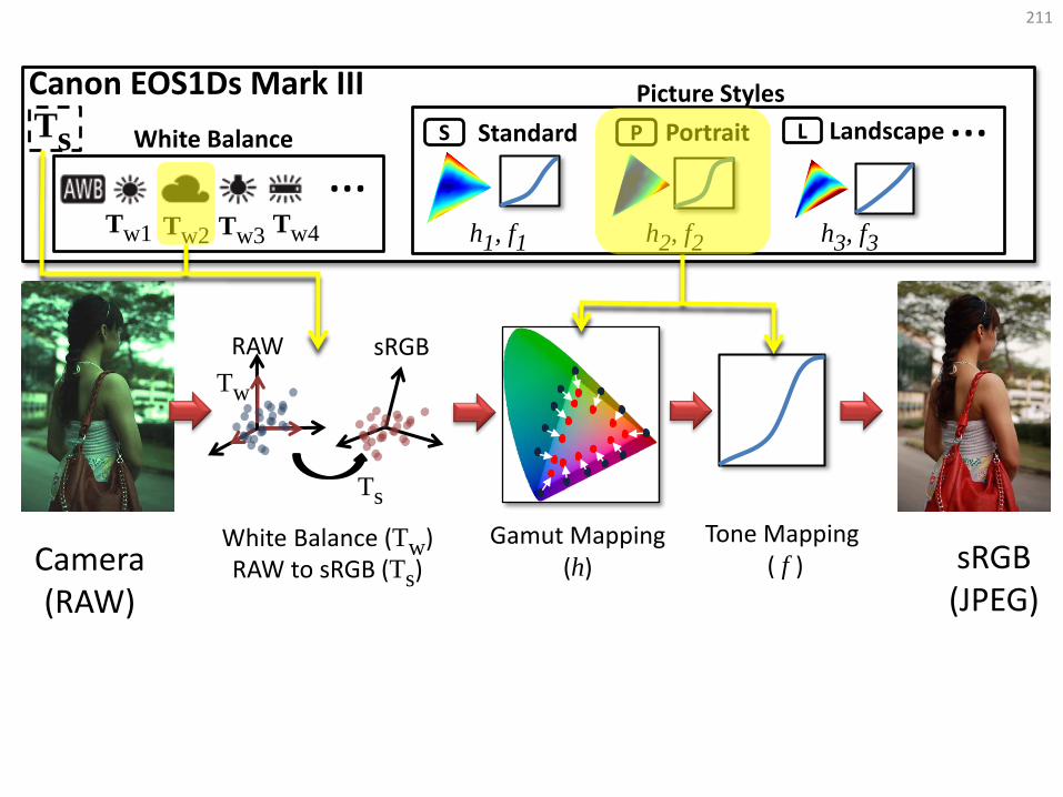
Canon EOS1Ds Mark III
……Ts
Tw1
White Balance
Picture Styles
h1, f1Tw2 Tw3
Tw4 h2, f2 h3, f3
RAW
RAW to sRGB (Ts)
Gamut Mapping (h)
Tone Mapping( f )
sRGB
Tw
Ts
White Balance (Tw)sRGB(JPEG)
Camera(RAW)
Standard Portrait LandscapeS P L
211

Canon EOS1Ds Mark III
……Ts
Tw1
White Balance
Picture Styles
h1, f1Tw2 Tw3
Tw4 h2, f2 h3, f3
RAW
RAW to sRGB (Ts)
Gamut Mapping (h)
Tone Mapping( f )
sRGB
Tw
Ts
White Balance (Tw)sRGB(JPEG)
Camera(RAW)
Standard Portrait LandscapeS P L
What if you took a photo with the wrong settings?
212
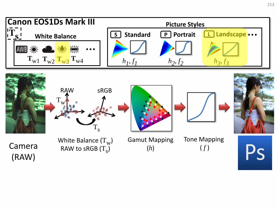
Canon EOS1Ds Mark III
……Ts
Tw1
White Balance
Picture Styles
h1, f1Tw2 Tw3
Tw4 h2, f2 h3, f3
RAW
sRGB(JPEG)
RAW to sRGB (Ts)
Gamut Mapping (h)
Tone Mapping( f )
sRGB
Tw
Ts
White Balance (Tw)Camera(RAW)
Standard Portrait LandscapeS P L
213
Canon EOS1Ds Mark III
……Ts
Tw1
White Balance
Picture Styles
h1, f1Tw2 Tw3
Tw4 h2, f2 h3, f3
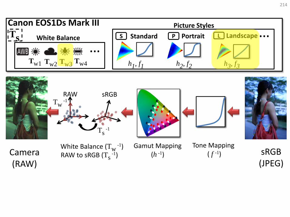
sRGB(JPEG)
Tone Mapping( f -1)
RAW
RAW to sRGB (Ts-1)
sRGBTw
-1
Ts-1
White Balance (Tw-1) Gamut Mapping
(h -1)Camera(RAW)
Standard Portrait LandscapeS P L
214
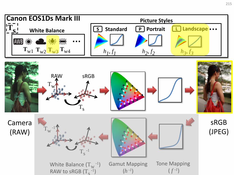
Canon EOS1Ds Mark III
……Ts
Tw1
White Balance
Picture Styles
h1, f1Tw2 Tw3
Tw4 h2, f2 h3, f3
sRGB(JPEG)
RAW to sRGB (Ts-1)
Gamut Mapping (h -1)
Tone Mapping( f -1)
Tw-1
Ts-1
White Balance (Tw-1)
RAW sRGB
Tw
Ts
Camera(RAW)
Standard Portrait LandscapeS P L
215
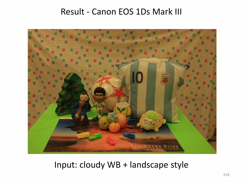
Input: cloudy WB + landscape style
Result - Canon EOS 1Ds Mark III
216
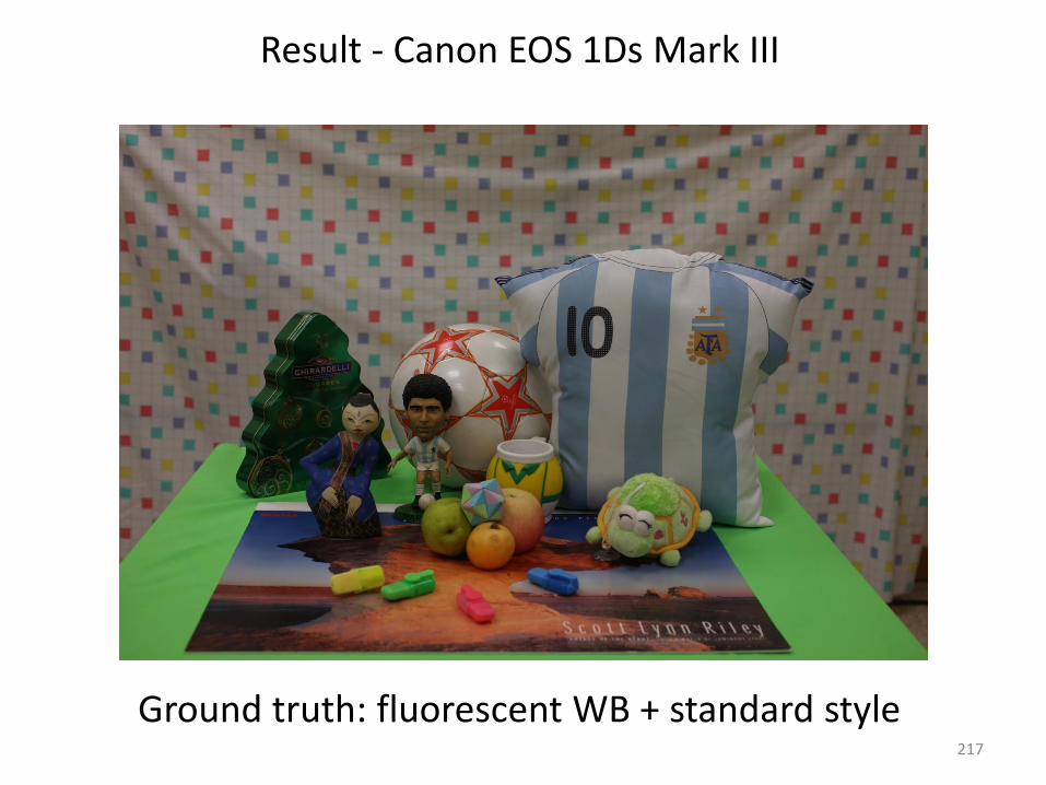
Ground truth: fluorescent WB + standard style
Result - Canon EOS 1Ds Mark III
217

Photoshop result
Result - Canon EOS 1Ds Mark III
218
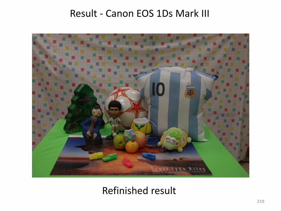
Refinished result
Result - Canon EOS 1Ds Mark III
219

Ground truth: fluorescent WB + standard style
Result - Canon EOS 1Ds Mark III
220
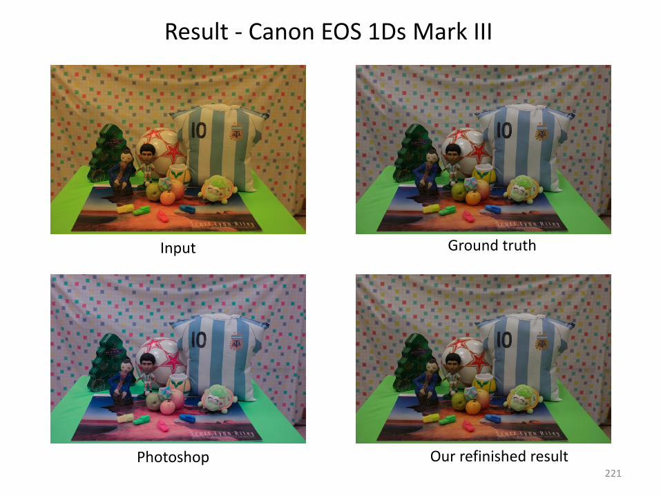
Input Ground truth
Our refinished resultPhotoshop
Result - Canon EOS 1Ds Mark III
221

Result - Canon EOS 1Ds Mark III
Input: tungsten WB + standard style222

Result - Canon EOS 1Ds Mark III
Ground truth: daylight WB + standard style223
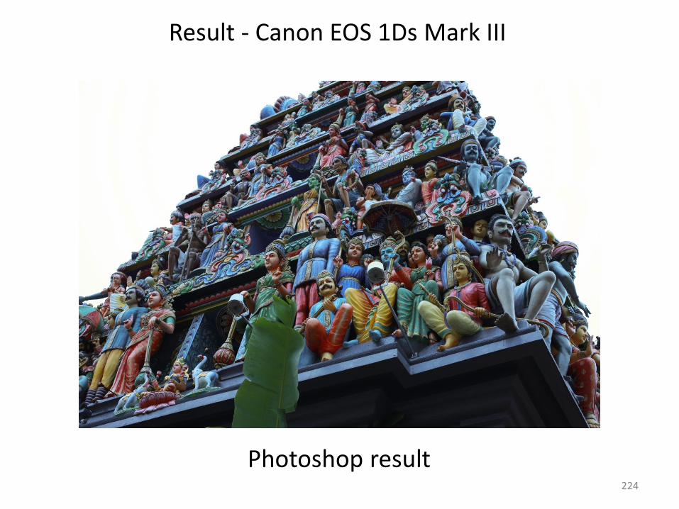
Result - Canon EOS 1Ds Mark III
Photoshop result224

Result - Canon EOS 1Ds Mark III
Our refinished result225

Result - Canon EOS 1Ds Mark III
Ground truth: daylight WB + standard style226

Input Ground truth
Our refinished resultPhotoshop
Result - Canon EOS 1Ds Mark III
227
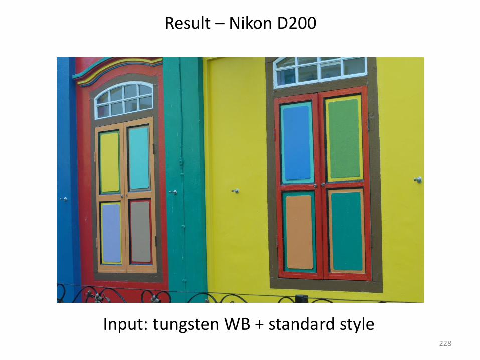
Result – Nikon D200
Input: tungsten WB + standard style228
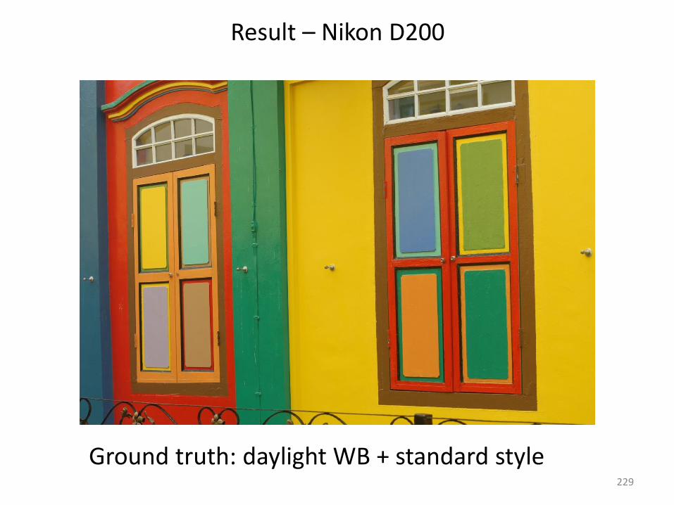
Result – Nikon D200
Ground truth: daylight WB + standard style229
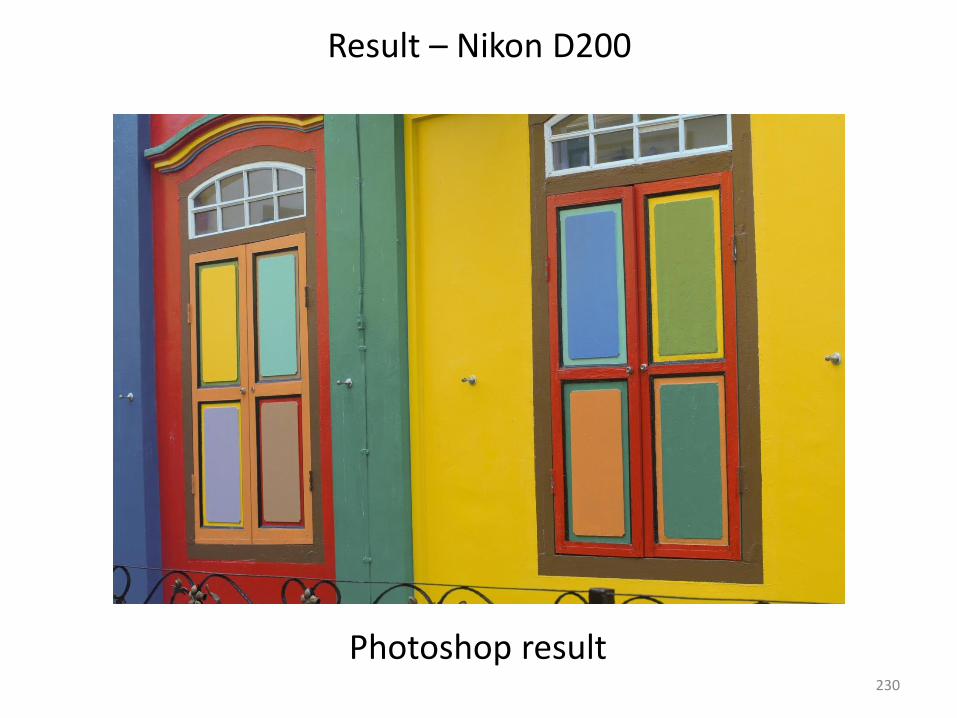
Result – Nikon D200
Photoshop result230

Result – Nikon D200
Refinished result231

Result – Nikon D200
Ground truth: daylight WB + standard style232

Input Ground truth
Photo refinishPhotoshop
Result – Nikon D200
233
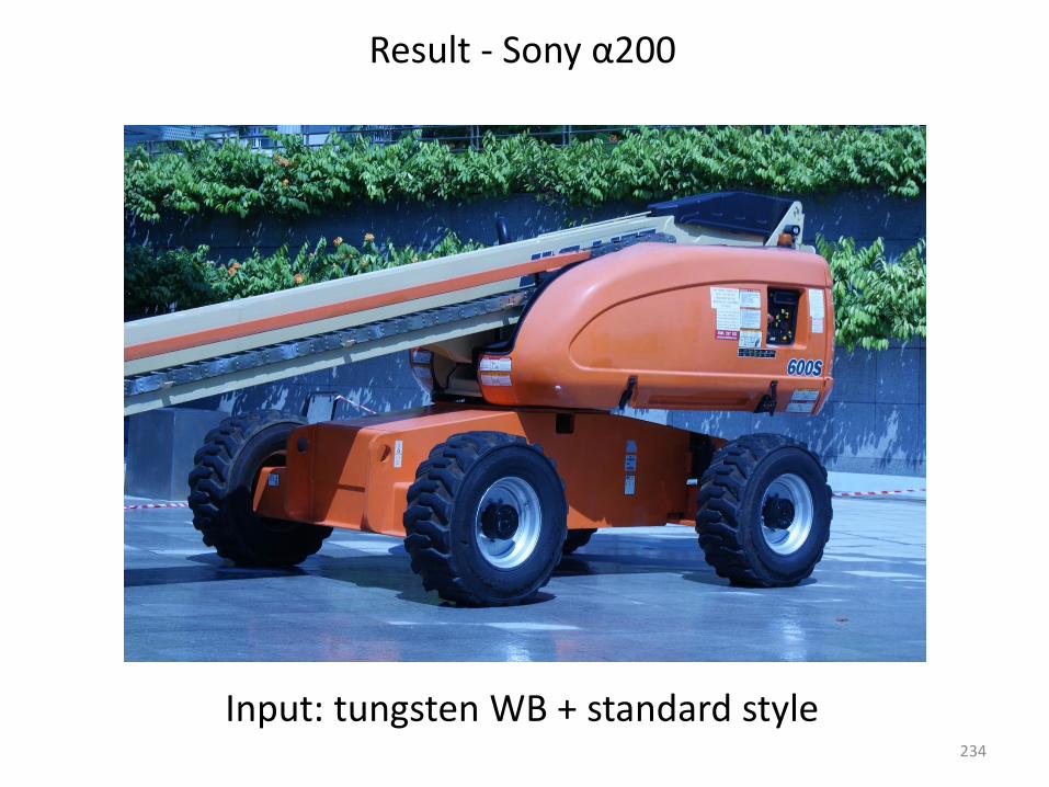
Result - Sony α200
Input: tungsten WB + standard style234
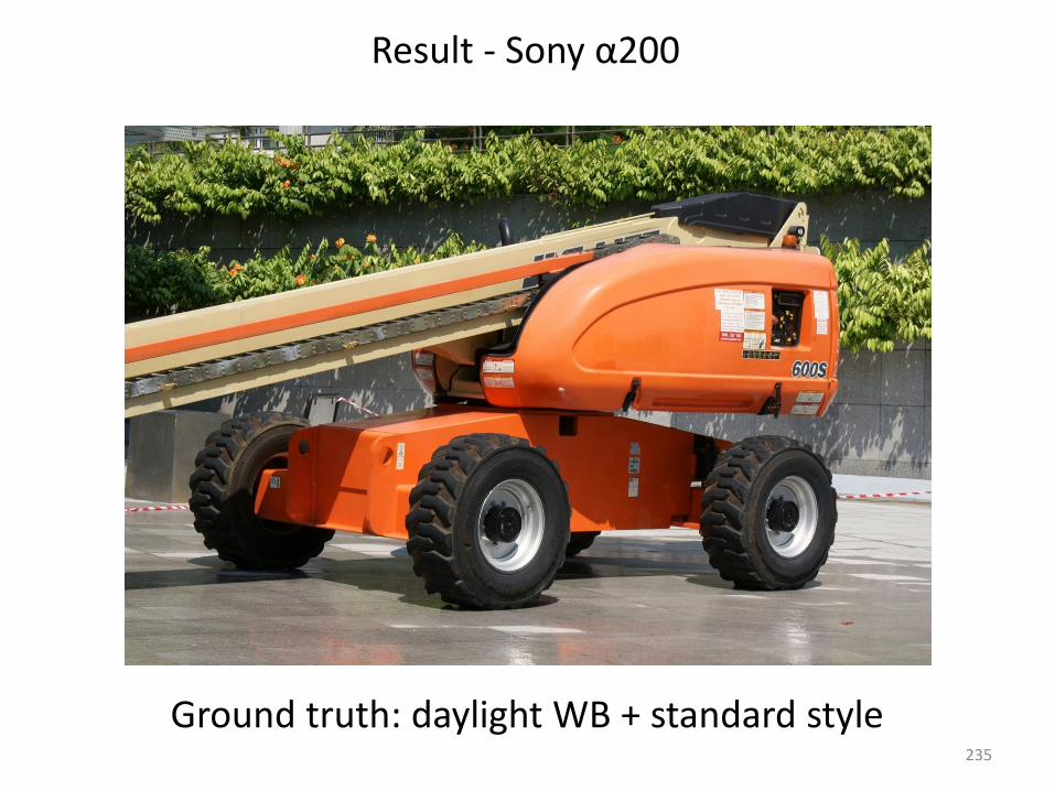
Result - Sony α200
Ground truth: daylight WB + standard style235
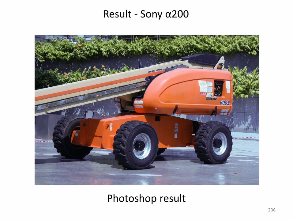
Result - Sony α200
Photoshop result236

Result - Sony α200
Our refinished result237

Result - Sony α200
Ground truth: daylight WB + standard style238
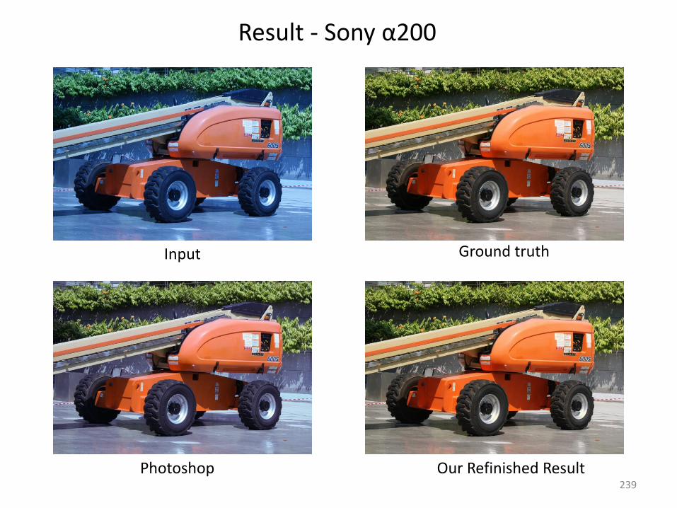
Input Ground truth
Our Refinished ResultPhotoshop
Result - Sony α200
239
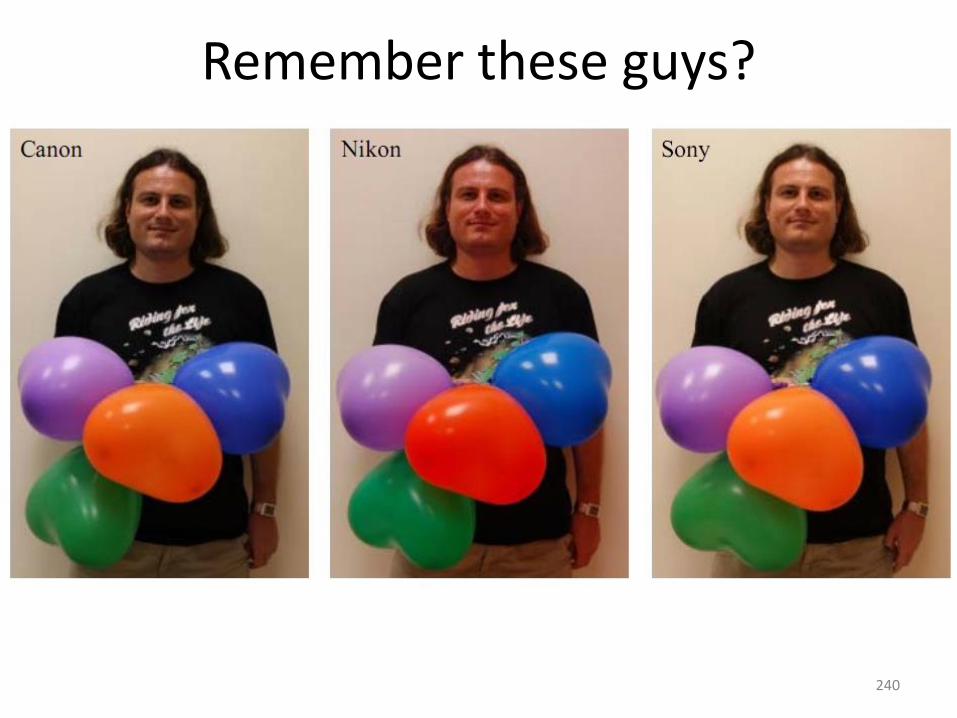
Remember these guys?
240
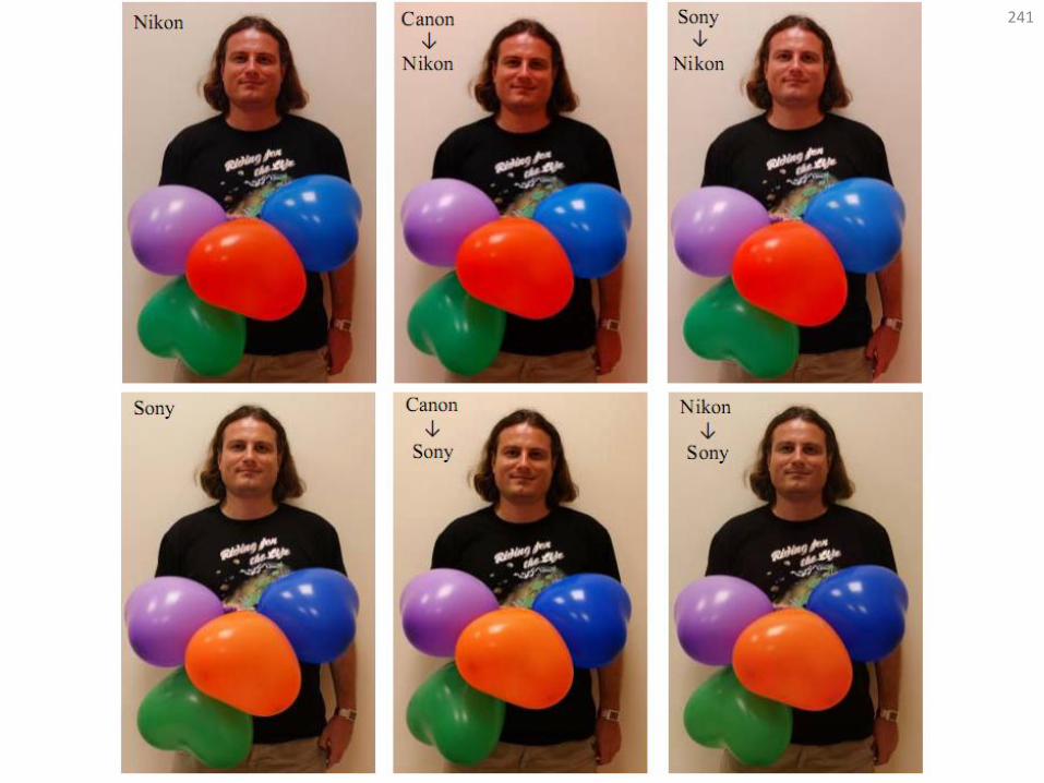
241
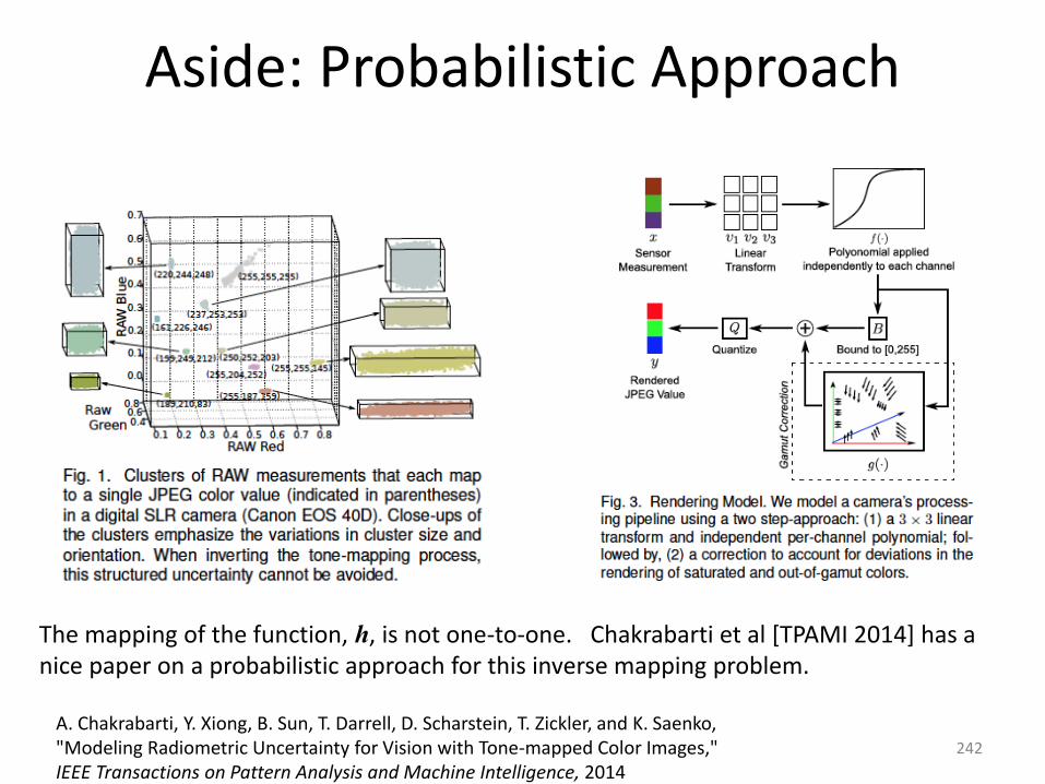
Aside: Probabilistic Approach
242
A. Chakrabarti, Y. Xiong, B. Sun, T. Darrell, D. Scharstein, T. Zickler, and K. Saenko, "Modeling Radiometric Uncertainty for Vision with Tone-mapped Color Images,"IEEE Transactions on Pattern Analysis and Machine Intelligence, 2014
The mapping of the function, h, is not one-to-one. Chakrabarti et al [TPAMI 2014] has a nice paper on a probabilistic approach for this inverse mapping problem.
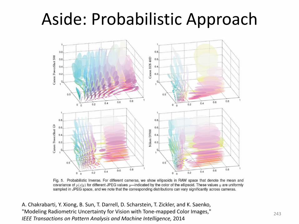
Aside: Probabilistic Approach
243
A. Chakrabarti, Y. Xiong, B. Sun, T. Darrell, D. Scharstein, T. Zickler, and K. Saenko, "Modeling Radiometric Uncertainty for Vision with Tone-mapped Color Images,"IEEE Transactions on Pattern Analysis and Machine Intelligence, 2014

Tutorial schedule
• Part 1 (General Part)
– Motivation
– Review of color/color spaces
– Overview of camera imaging pipeline
• Part 2 (Specific Part)
– Modeling the in-camera color pipeline
– Photo-refinishing
• Part 3 (Wrap Up)
– The good, the bad, and the ugly of commodity cameras and computer vision research
– Concluding Remarks
244

Part 3: Wrap Up
245
The Good, The Bad, and the Ugly - 1966Western Movie directed by Sergio LeoneOne of the most influential “Western” films and one of the “Great Films of All Times”
Image Credit: Timothy Anderson
246

247
Color on cameras is not standard
• We have already discussed the “bad” in part 2
• No camera outputs true “sRGB” with respect to the incoming light
• Each camera applies its own color rendering
• Calibration of the camera is required
• While we have good calibration methods, such calibration needs to be done for each camera, and for many different settings (not practical)
248
No standard for RAW color space
• RAW is good because it is linear
• However, RAW is a scene-referred color space, specific to the sensor
• This mean RAW RGB values from image on difference cameras of the same scene will be different
249

Example – RAW is not standard
250
ExampleTop: RAW images from three cameras, all of the same scene.Bot: Error plots showing the pixel-wise L2 difference between camera pairs

251
Problems in academic research
1. Lack of understanding of color on cameras and relationship to “real” color spaces
2. Research and results performed “out of context” of the camera processing pipeline
3. Lack of ability to emulate full camera pipelines
252

Ugly Example – Color spaces
• Recall our color space transforms
• Camera images are saved in sRGB
253
Linear-sRGB back to XYZ
Linear-NTSC back to XYZ
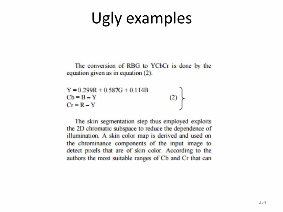
Ugly examples
254
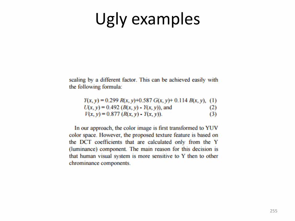
Ugly examples
255

Ugly examples
256

Analyzing ugly
• One of the most common examples in the academic literature – obtaining the luminance (CIE Y) channel from an sRGB image
• Goal is to often purported to find the imaged scene’s “brightness” (i.e. CIE Y)
sRGB CIE Y
257

Analyzing sRGB to luminance (Y)
1) Perform experiments to see just how accurate sRGB to luminance conversion
2) Examine the common mistakes made in the academic literature
258
400 500 600 7000
0.5
1
1.5
2
2.5
X
YZ
YX
Z
Color Matching FunctionsCIE XYZ
Image under CIE XYZ color space
SPD2 (Y:38, x:0.24, y:0.61)
SPD1 (Y:50, x:0.56, y:0.37) 𝑥
y
Y (Luminance)
0
Chromaticity
Scene (Spectral Power Distribution)
400 500 600 700
SPD1
400 500 600 700
SPD2
𝑆(x, 𝜆)
𝐶𝑐(𝜆) CIE XYZ
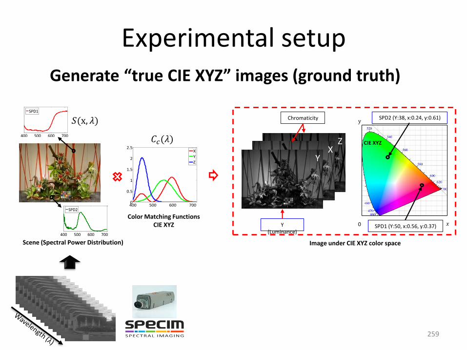
Experimental setupGenerate “true CIE XYZ” images (ground truth)
259

Test on two types of inputs
400 500 600 700
SPD1
400 500 600 700
SPD2
𝑆(x, 𝜆)
Color rendition chart Full scenes
260
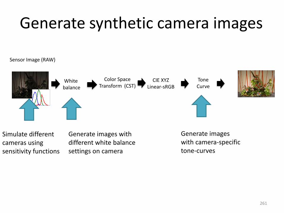
Generate synthetic camera images
Sensor Image (RAW)
White balance
Color Space Transform (CST)
CIE XYZLinear-sRGB
ToneCurve
Simulate differentcameras usingsensitivity functions
Generate images withdifferent white balancesettings on camera
Generate imageswith camera-specifictone-curves
261

Three common mistakes in the literature
• Assumption that white balance is correct
• Using the wrong equations (and calling it CIE Y)
• Not applying the correct linearization step
(when attempting to map a sRGB camera image to CIE – Y)
262

1. White balance assumption
Sensor Image (RAW)
Whitebalance
Color Space Transform (CST)
CIE XYZLinear-sRGB
ToneCurve
There is an implicit assumptionthat the white balance was
estimated correctly
263
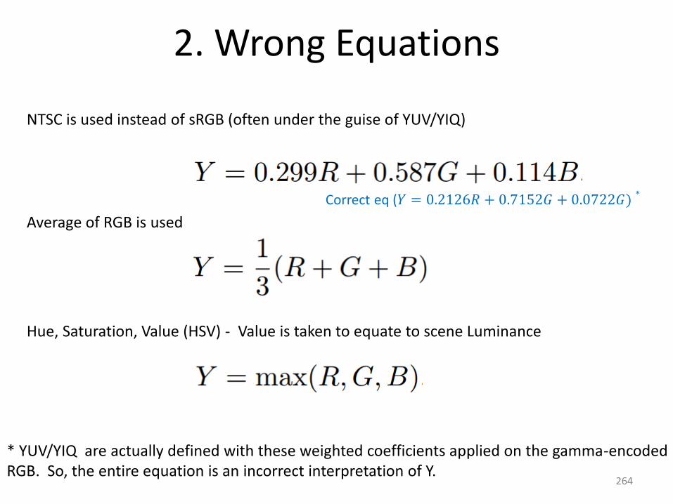
2. Wrong Equations
NTSC is used instead of sRGB (often under the guise of YUV/YIQ)
Average of RGB is used
Hue, Saturation, Value (HSV) - Value is taken to equate to scene Luminance
Correct eq (𝑌 = 0.2126𝑅 + 0.7152𝐺 + 0.0722𝐺)∗
264
* YUV/YIQ are actually defined with these weighted coefficients applied on the gamma-encodedRGB. So, the entire equation is an incorrect interpretation of Y.
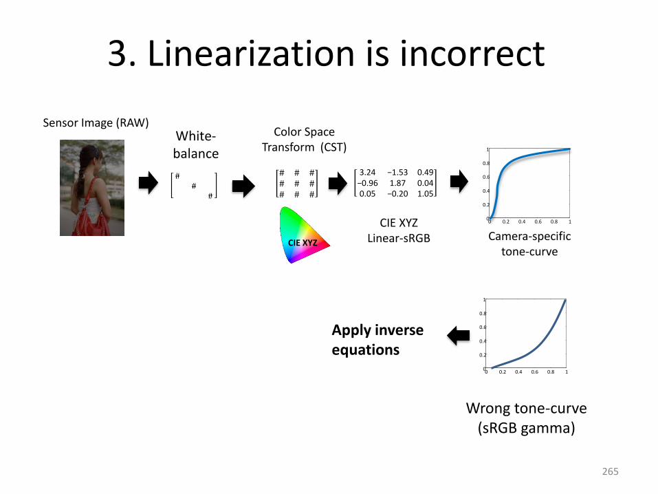
3. Linearization is incorrect
Sensor Image (RAW)White-balance
Color Space Transform (CST)
CIE XYZ
CIE XYZLinear-sRGB
3.24 −1.53 0.49−0.96 1.87 0.040.05 −0.20 1.05
0 0.2 0.4 0.6 0.8 10
0.2
0.4
0.6
0.8
1
0 0.2 0.4 0.6 0.8 10
0.2
0.4
0.6
0.8
1
Wrong tone-curve(sRGB gamma)
Apply inverseequations
Camera-specifictone-curve
265
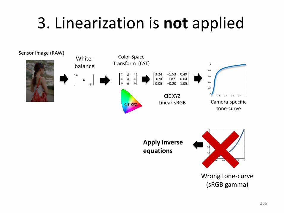
3. Linearization is not applied
Sensor Image (RAW)White-balance
Color Space Transform (CST)
CIE XYZ
CIE XYZLinear-sRGB
3.24 −1.53 0.49−0.96 1.87 0.040.05 −0.20 1.05
0 0.2 0.4 0.6 0.8 10
0.2
0.4
0.6
0.8
1
0 0.2 0.4 0.6 0.8 10
0.2
0.4
0.6
0.8
1
Wrong tone-curve(sRGB gamma)
Apply inverseequations
Camera-specifictone-curve
266
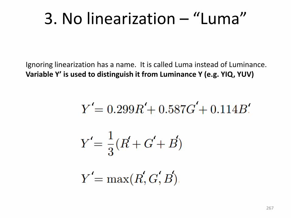
3. No linearization – “Luma”
Ignoring linearization has a name. It is called Luma instead of Luminance. Variable Y’ is used to distinguish it from Luminance Y (e.g. YIQ, YUV)
‘ ‘ ‘ ‘
‘ ‘ ‘‘
‘ ‘ ‘‘
267

How ugly is it?
268
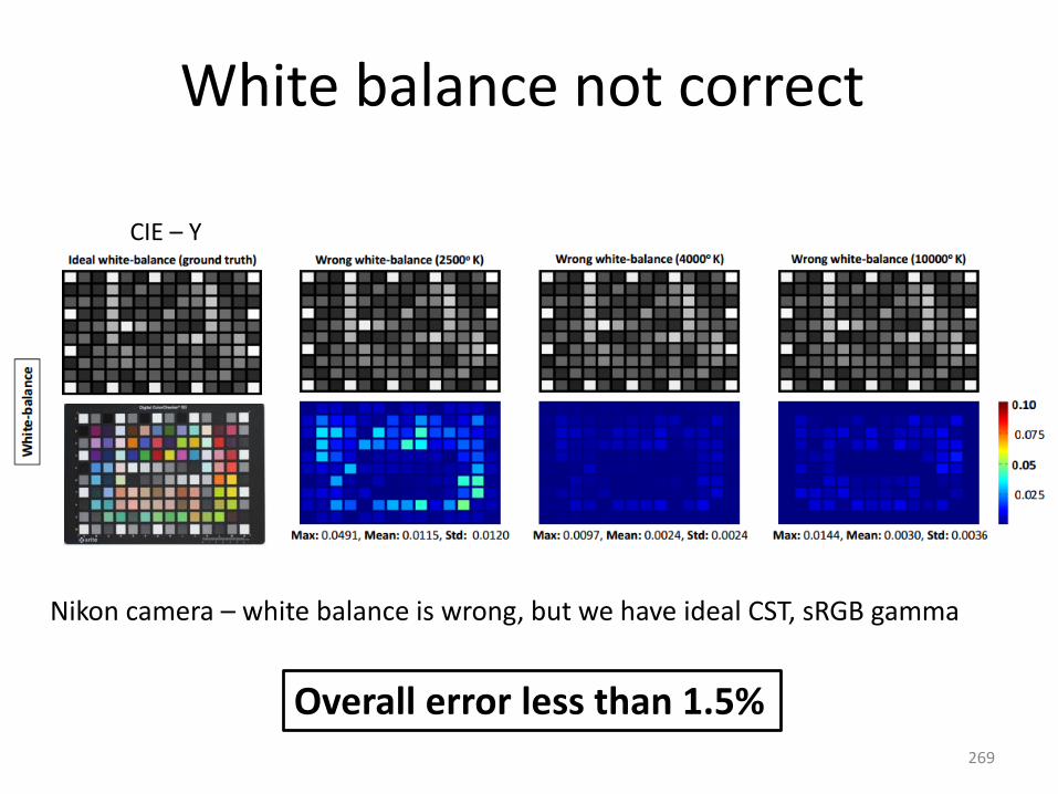
White balance not correct
Nikon camera – white balance is wrong, but we have ideal CST, sRGB gamma
Overall error less than 1.5%
CIE – Y
269
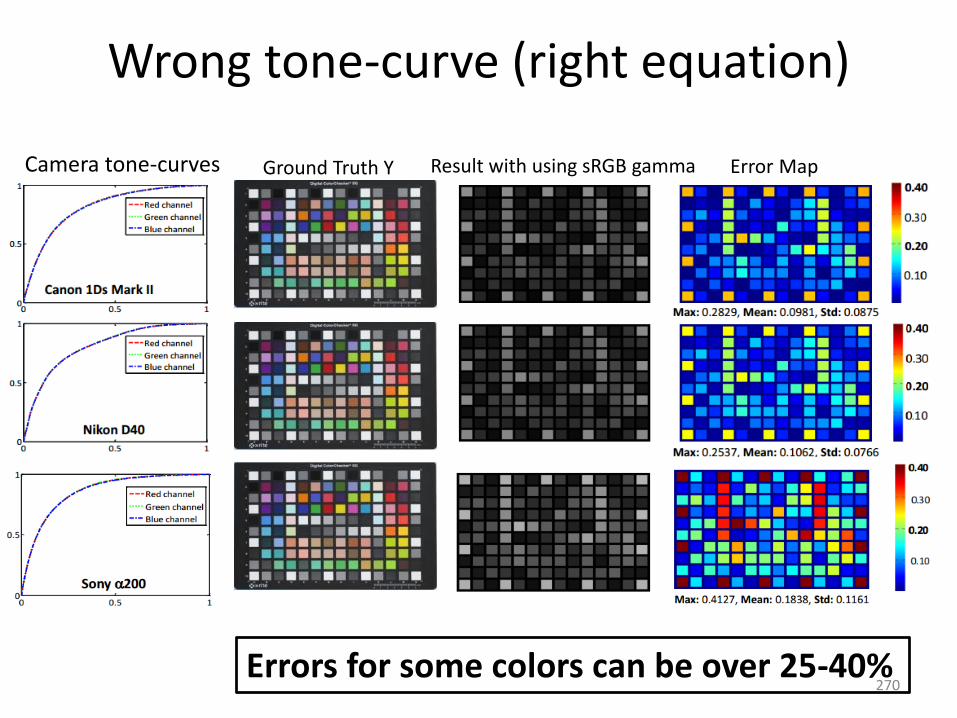
Wrong tone-curve (right equation)
Camera tone-curves Ground Truth Y Result with using sRGB gamma
Errors for some colors can be over 25-40%
Error Map
270
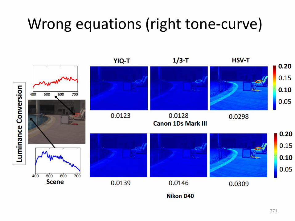
Wrong equations (right tone-curve)
271
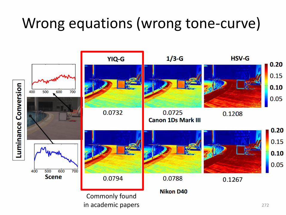
Wrong equations (wrong tone-curve)
Commonly foundin academic papers 272
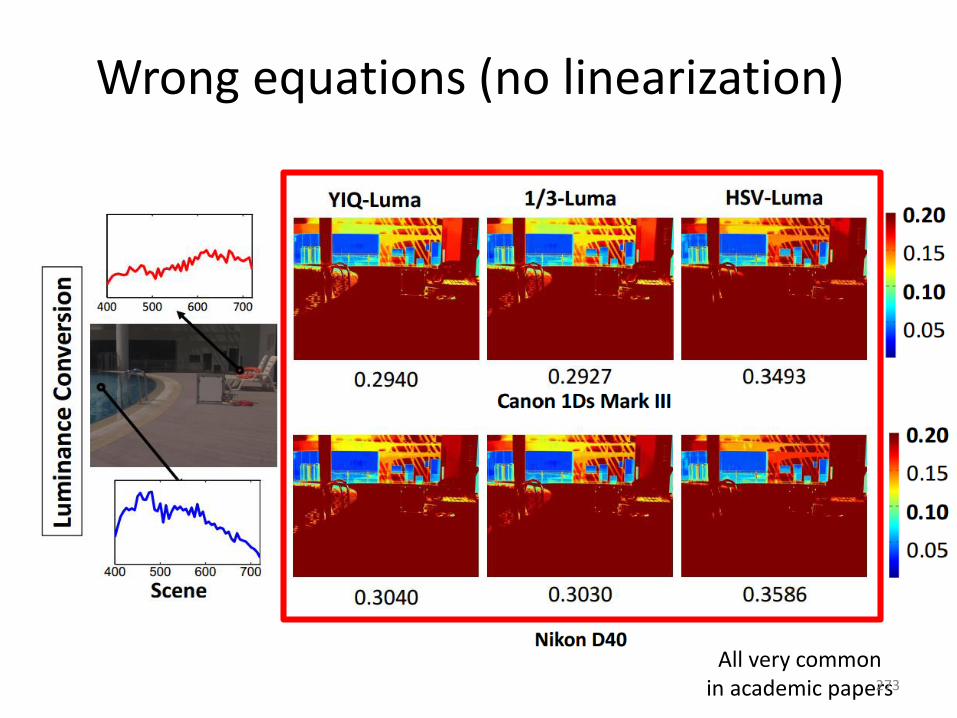
Wrong equations (no linearization)
All very commonin academic papers273
Ugly analysis
• White balance assumption violation not too serious
• Incorrect tone-curve is significant (25-40% error)
• No tone-curve (Luma) is the worse (over 40% error)
• HSV is the worst of the “wrong” equations,but not worse than using the incorrect tone-curve
274

(a) sRGB image (b) Y of YIQ (c) RGB to Gray*
(d) SIFT features on (b) (e) SIFT features on (c)
SIFT
Canny
(f) Canny edges on (b) (g) Canny edges on (c)
Why bother with CIE-Y?
*C. Lu, et al “Contrast preserving decolorization with perception-based quality metrics”, IJCV, 2014275
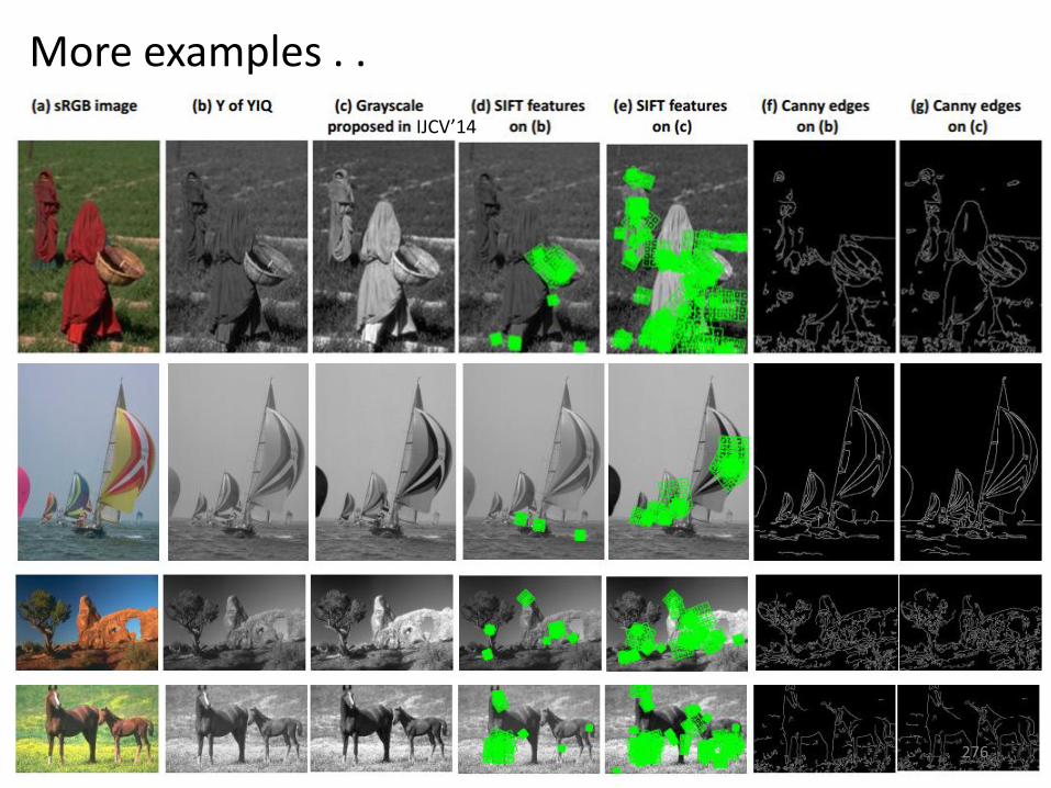
More examples . .
276
IJCV’14

Another ugly problem . . .
• Applying operations in the “wrong” context . . .
• E.g. applying white balance on sRGB images . . .
• Or, denoising an sRGB image. . .
• Or, deblurring an sRGB image . . .
277
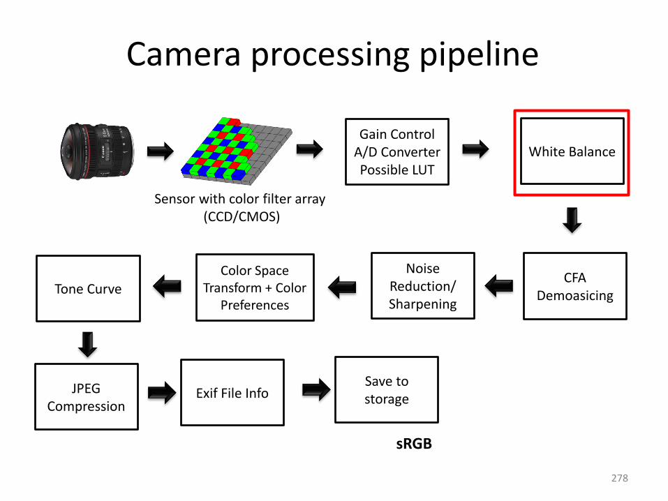
Camera processing pipeline
Gain ControlA/D ConverterPossible LUT
Sensor with color filter array (CCD/CMOS)
CFADemoasicing
White Balance
Color Space Transform + Color
PreferencesTone Curve
JPEG Compression
Exif File Info
Noise Reduction/Sharpening
Save to storage
sRGB
278

Classic white balance results out-of-context
From Cheng et al CVPR 2015
“Subjective” white balance results shown(images are in camera-raw color space)
279
These subjective results have absolutely no visual meaning.The camera-raw is not a standard color space!

Consider image deblurring
Assumption is: linear color space (RAW or linear-sRGB)
Reality: image has been run through the pipeline and some non-linear tone-curve f
280
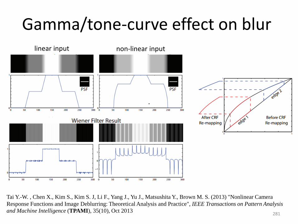
Gamma/tone-curve effect on blur linear input non-linear input
281
∙
Tai Y.-W. , Chen X., Kim S., Kim S. J, Li F., Yang J., Yu J., Matsushita Y., Brown M. S. (2013) "Nonlinear Camera
Response Functions and Image Deblurring: Theoretical Analysis and Practice", IEEE Transactions on Pattern Analysis
and Machine Intelligence (TPAMI), 35(10), Oct 2013

RAW vs sRGB deblurring
Input with blur Ground Truth Deblur on RAW Deblur on sRGB
282

State of affairs (The Ugly)
• Many researchers don’t understand camera color
• Attempt to treat sRGB images as true scene measurements (ideal sRGB images)– Often use wrong equations, forget linearization, etc. . – Results can be erroneous by up to 50%– Why even attempt CIE Y?
• Research is often applied without understanding the context of the color processing pipeline
283
284
285
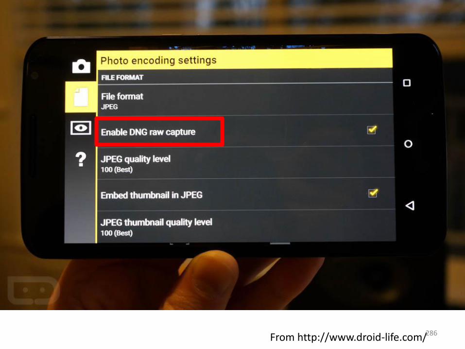
From http://www.droid-life.com/286

Adobe Digital Negative (DNG)
• Public raw-camera image file specification
• Open source SDK for processing DNG to sRGB
• After almost 10 years, this is becoming mainstream
287
Android Camera2 API
• Allows access to many of the onboard camera procedures
• Access to camera characteristics (CST, white balance)
• Can capture RAW images in DNG format
288
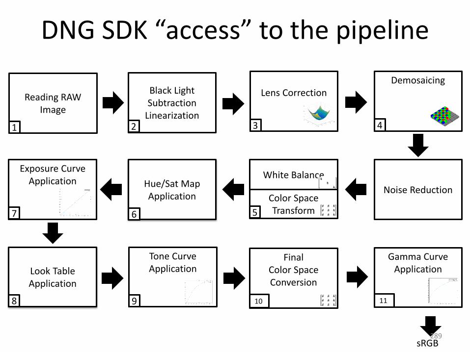
DNG SDK “access” to the pipeline
sRGB
White Balance
Color Space Transform
Hue/Sat Map Application
Reading RAW Image
Black Light Subtraction
Linearization
Lens CorrectionDemosaicing
Exposure Curve Application
Look Table Application
Tone Curve Application
Final Color Space Conversion
Gamma Curve Application
Noise Reduction
1 3 4
57
2
8 9 10
6
11
289
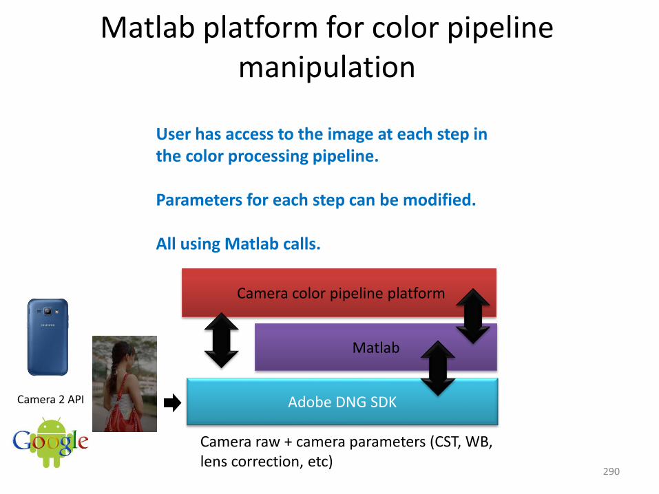
Matlab platform for color pipeline manipulation
Matlab
Adobe DNG SDK
Camera color pipeline platform
Camera 2 API
Camera raw + camera parameters (CST, WB,lens correction, etc)
User has access to the image at each step in the color processing pipeline.
Parameters for each step can be modified.
All using Matlab calls.
290
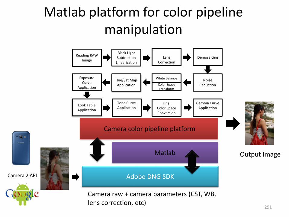
Matlab platform for color pipeline manipulation
Matlab
Adobe DNG SDK
Camera color pipeline platform
Camera 2 API
Output Image
Camera raw + camera parameters (CST, WB,lens correction, etc)
White Balance
Color Space Transform
Hue/Sat Map Application
Reading RAW Image
Black Light Subtraction
Linearization
Lens Correction
Demosaicing
Exposure Curve
Application
Look Table Application
Tone Curve Application
Final Color Space Conversion
Gamma Curve Application
Noise Reduction
291
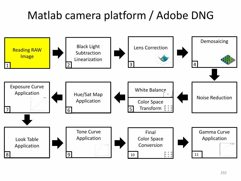
Matlab camera platform / Adobe DNG
White Balance
Color Space Transform
Hue/Sat Map Application
Reading RAW Image
Black Light Subtraction
Linearization
Lens CorrectionDemosaicing
Exposure Curve Application
Look Table Application
Tone Curve Application
Final Color Space Conversion
Gamma Curve Application
Noise Reduction
1 3 4
57
2
8 9 10
6
11
292

Reading RAW Image
293

Matlab camera platform / Adobe DNG
White Balance
Color Space Transform
Hue/Sat Map Application
Reading RAW Image
Black Light Subtraction
Linearization
Lens CorrectionDemosaicing
Exposure Curve Application
Look Table Application
Tone Curve Application
Final Color Space Conversion
Gamma Curve Application
Noise Reduction
1 3 4
57
2
8 9 10
6
11
294

Black light subtraction + linearization
295
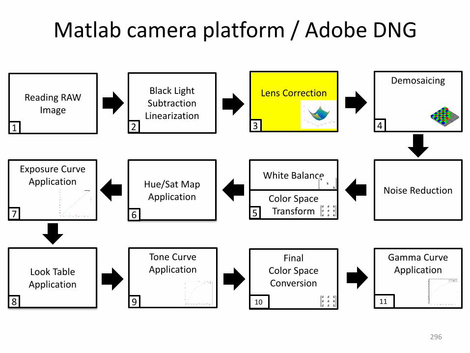
Matlab camera platform / Adobe DNG
White Balance
Color Space Transform
Hue/Sat Map Application
Reading RAW Image
Black Light Subtraction
Linearization
Lens CorrectionDemosaicing
Exposure Curve Application
Look Table Application
Tone Curve Application
Final Color Space Conversion
Gamma Curve Application
Noise Reduction
1 3 4
57
2
8 9 10
6
11
296
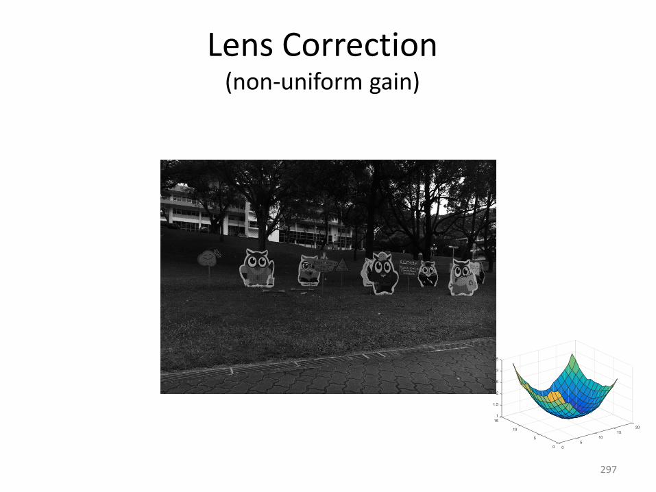
Lens Correction(non-uniform gain)
297

Matlab camera platform / Adobe DNG
White Balance
Color Space Transform
Hue/Sat Map Application
Reading RAW Image
Black Light Subtraction
Linearization
Lens CorrectionDemosaicing
Exposure Curve Application
Look Table Application
Tone Curve Application
Final Color Space Conversion
Gamma Curve Application
Noise Reduction
1 3 4
57
2
8 9 10
6
11
298
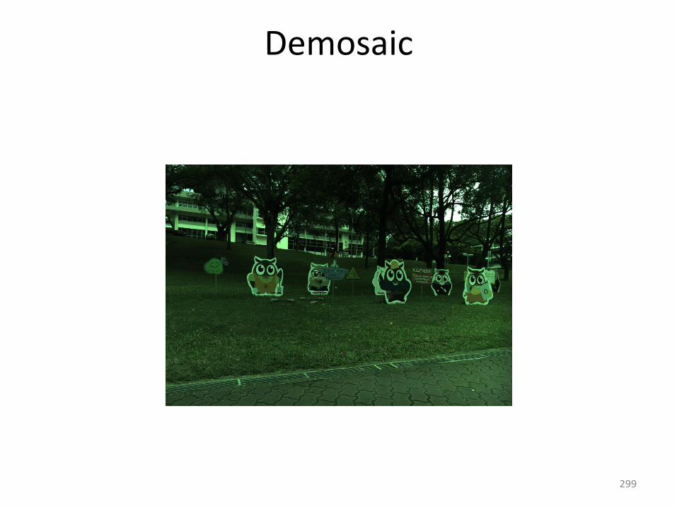
Demosaic
299

Matlab camera platform / Adobe DNG
White Balance
Color Space Transform
Hue/Sat Map Application
Reading RAW Image
Black Light Subtraction
Linearization
Lens CorrectionDemosaicing
Exposure Curve Application
Look Table Application
Tone Curve Application
Final Color Space Conversion
Gamma Curve Application
Noise Reduction
1 3 4
57
2
8 9 10
6
11
300

White balance + color space transform
301
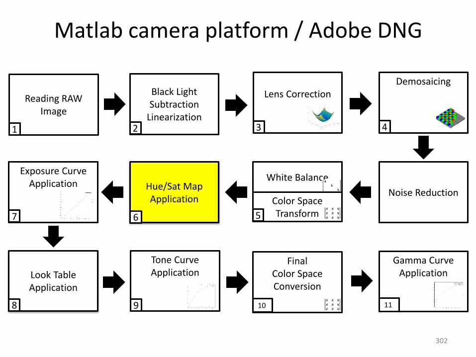
Matlab camera platform / Adobe DNG
White Balance
Color Space Transform
Hue/Sat Map Application
Reading RAW Image
Black Light Subtraction
Linearization
Lens CorrectionDemosaicing
Exposure Curve Application
Look Table Application
Tone Curve Application
Final Color Space Conversion
Gamma Curve Application
Noise Reduction
1 3 4
57
2
8 9 10
6
11
302
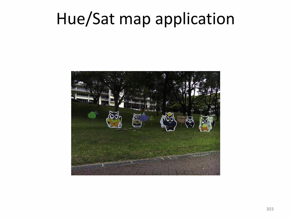
Hue/Sat map application
303
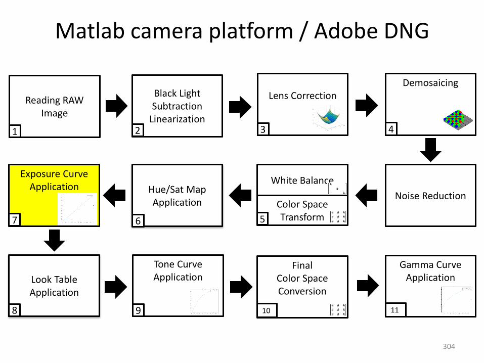
Matlab camera platform / Adobe DNG
White Balance
Color Space Transform
Hue/Sat Map Application
Reading RAW Image
Black Light Subtraction
Linearization
Lens CorrectionDemosaicing
Exposure Curve Application
Look Table Application
Tone Curve Application
Final Color Space Conversion
Gamma Curve Application
Noise Reduction
1 3 4
57
2
8 9 10
6
11
304
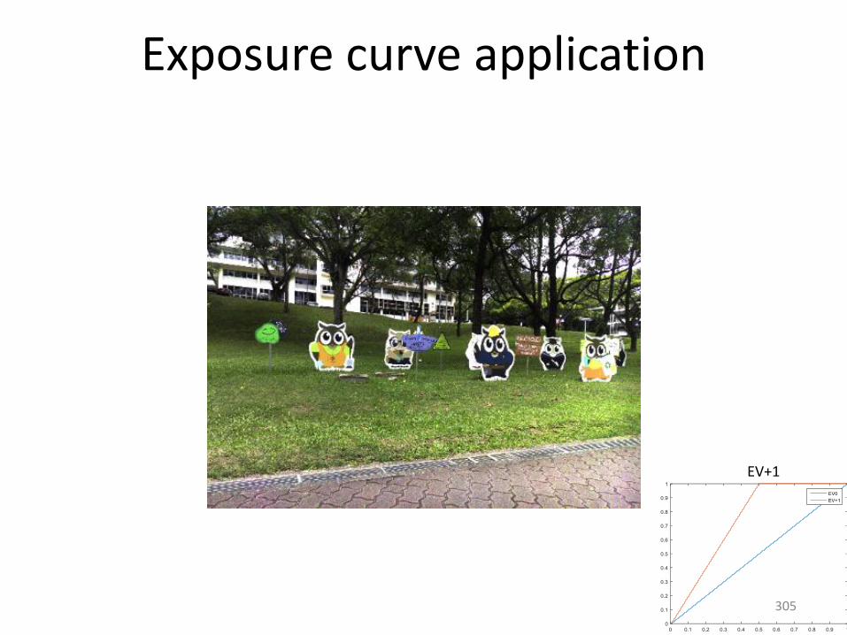
Exposure curve application
EV+1
305
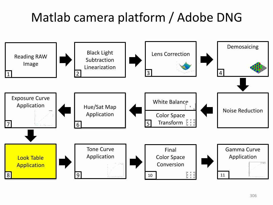
Matlab camera platform / Adobe DNG
White Balance
Color Space Transform
Hue/Sat Map Application
Reading RAW Image
Black Light Subtraction
Linearization
Lens CorrectionDemosaicing
Exposure Curve Application
Look Table Application
Tone Curve Application
Final Color Space Conversion
Gamma Curve Application
Noise Reduction
1 3 4
57
2
8 9 10
6
11
306
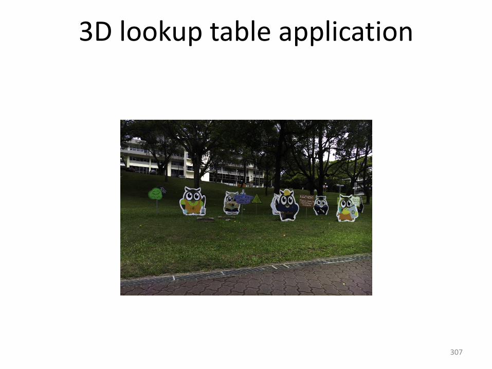
3D lookup table application
307
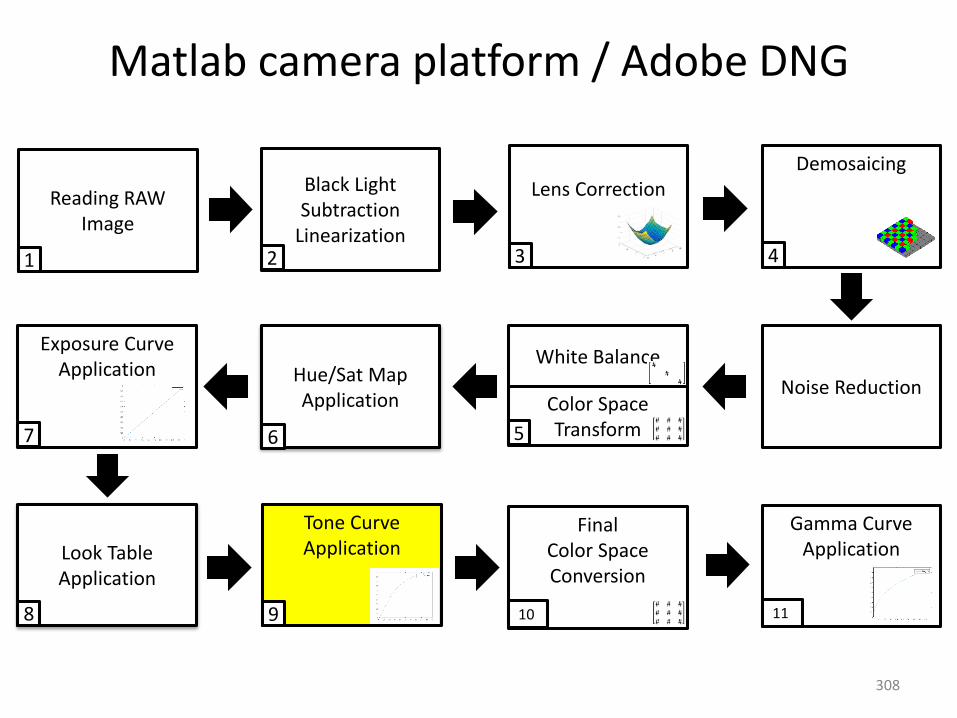
Matlab camera platform / Adobe DNG
White Balance
Color Space Transform
Hue/Sat Map Application
Reading RAW Image
Black Light Subtraction
Linearization
Lens CorrectionDemosaicing
Exposure Curve Application
Look Table Application
Tone Curve Application
Final Color Space Conversion
Gamma Curve Application
Noise Reduction
1 3 4
57
2
8 9 10
6
11
308

Tone curve application
309

Matlab camera platform / Adobe DNG
White Balance
Color Space Transform
Hue/Sat Map Application
Reading RAW Image
Black Light Subtraction
Linearization
Lens CorrectionDemosaicing
Exposure Curve Application
Look Table Application
Tone Curve Application
Final Color Space Conversion
Gamma Curve Application
Noise Reduction
1 3 4
57
2
8 9 10
6
11
310
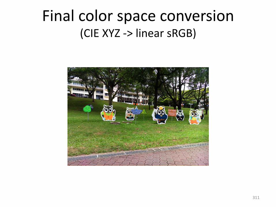
Final color space conversion(CIE XYZ -> linear sRGB)
311

Matlab camera platform / Adobe DNG
White Balance
Color Space Transform
Hue/Sat Map Application
Reading RAW Image
Black Light Subtraction
Linearization
Lens CorrectionDemosaicing
Exposure Curve Application
Look Table Application
Tone Curve Application
Final Color Space Conversion
Gamma Curve Application
Noise Reduction
1 3 4
57
2
8 9 10
6
11
312
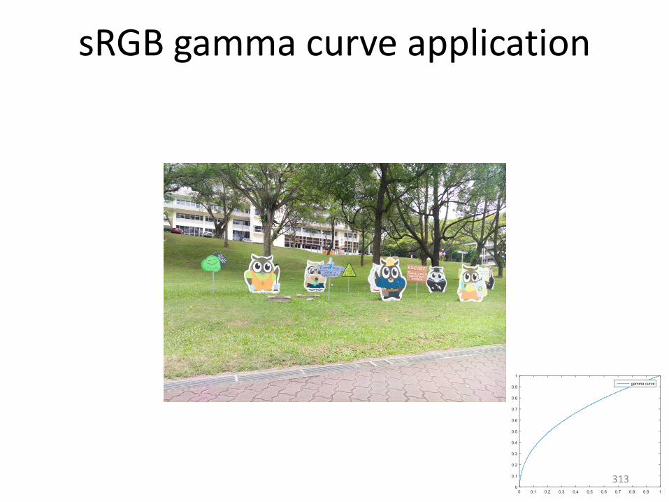
sRGB gamma curve application
313
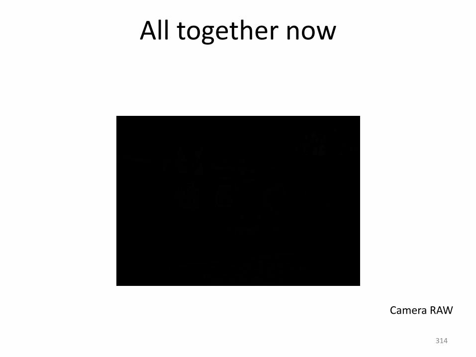
All together now
Camera RAW
314

All together now
Black level subtraction andlinearization315
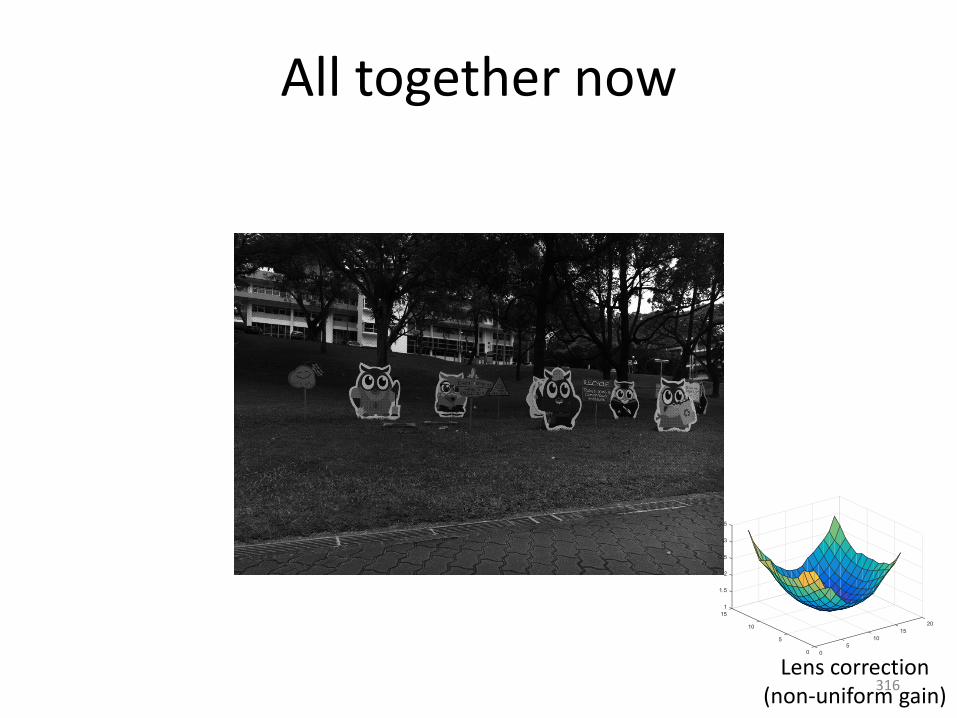
All together now
Lens correction(non-uniform gain)
316

All together now
Demosaicing+ Noise Reduction
317
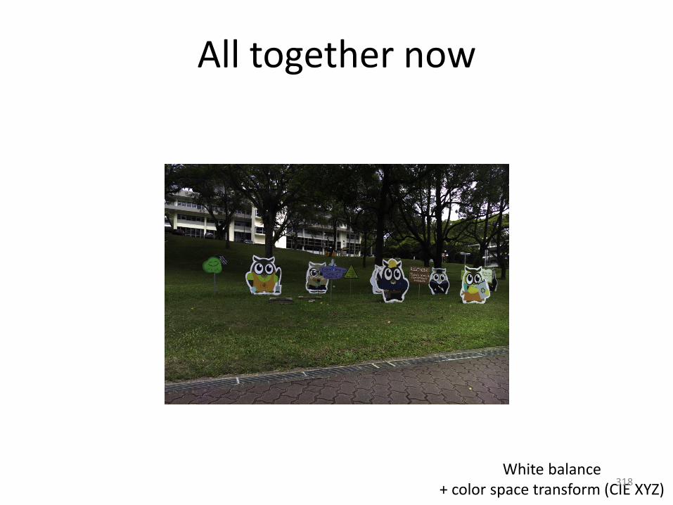
All together now
White balance+ color space transform (CIE XYZ)
318
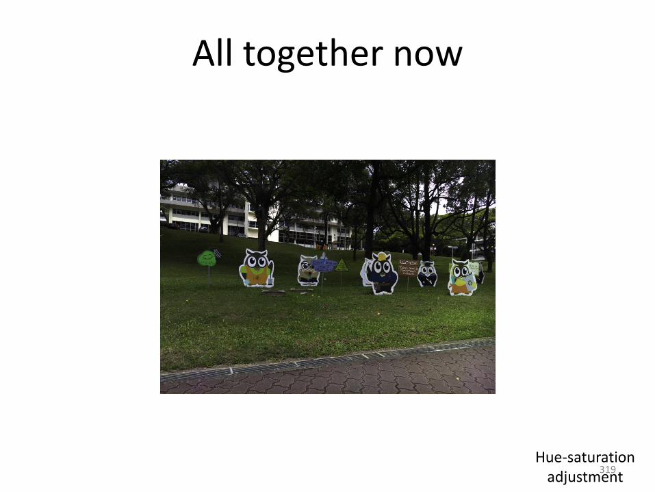
All together now
Hue-saturationadjustment
319

All together now
ExposureCompensation
320

All together now
Tone-Curve 321
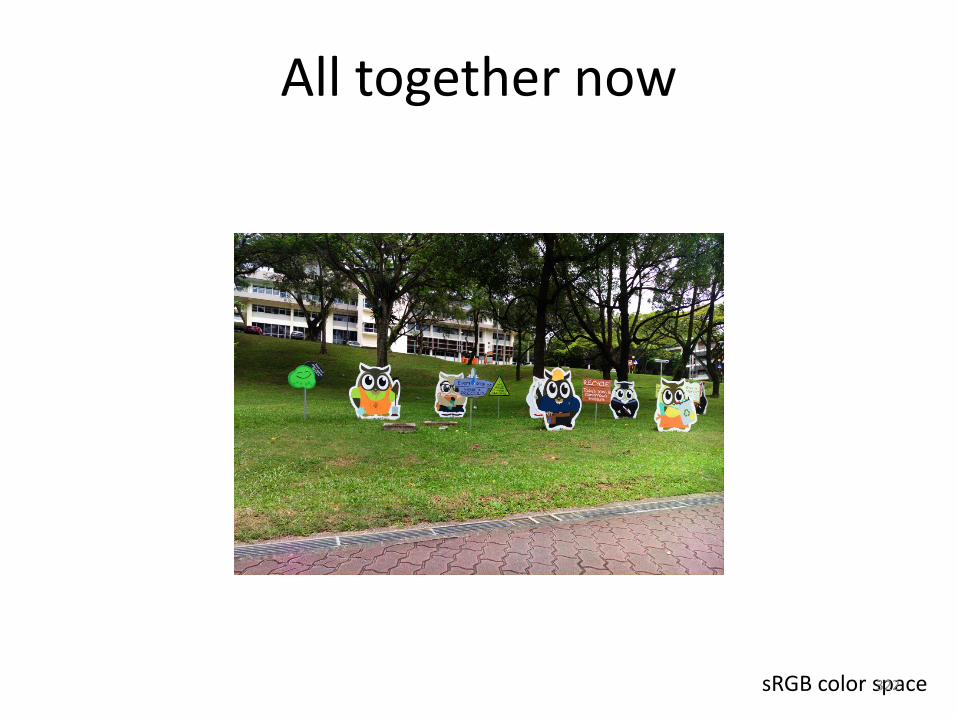
All together now
sRGB color space322
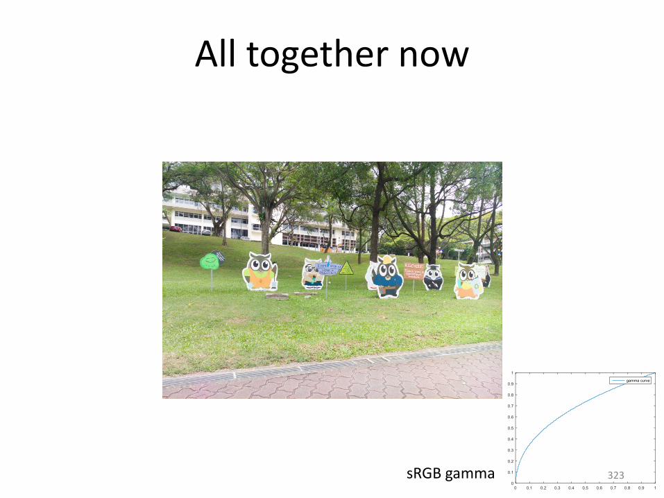
All together now
sRGB gamma 323
Using the platform - Examples
• White balance “in context”
• Camera colorimetry
• Real sRGB outputs
324
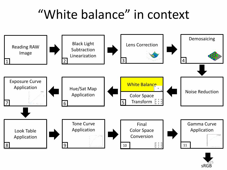
“White balance” in context
sRGB
White Balance
Color Space Transform
Hue/Sat Map Application
Reading RAW Image
Black Light Subtraction
Linearization
Lens CorrectionDemosaicing
Exposure Curve Application
Look Table Application
Tone Curve Application
Final Color Space Conversion
Gamma Curve Application
Noise Reduction
1 3 4
57
2
8 9 10
6
11
325
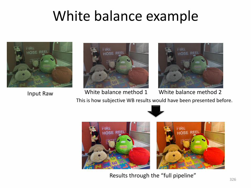
White balance example
Input Raw White balance method 1 White balance method 2
This is how subjective WB results would have been presented before.
Results through the “full pipeline”326
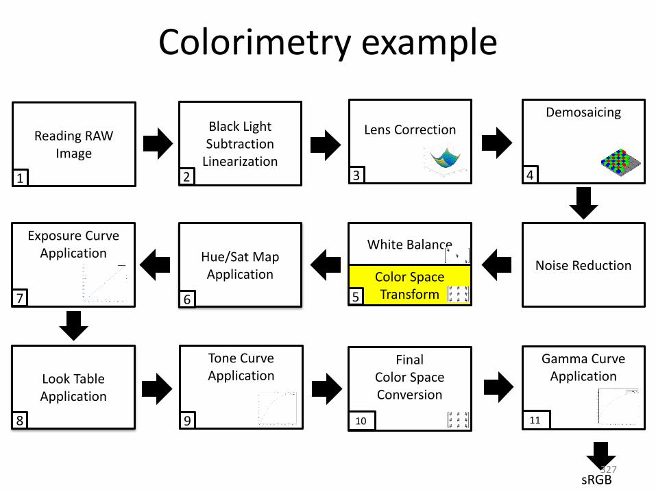
Colorimetry example
sRGB
White Balance
Color Space Transform
Hue/Sat Map Application
Reading RAW Image
Black Light Subtraction
Linearization
Lens CorrectionDemosaicing
Exposure Curve Application
Look Table Application
Tone Curve Application
Final Color Space Conversion
Gamma Curve Application
Noise Reduction
1 3 4
57
2
8 9 10
6
11
327

Example - colorimetry
Sensor Image (RAW)White
balance
Color Space Transform (CST)
CIE XYZ
CIE XYZLinear-sRGB
3.24 −1.53 0.49−0.96 1.87 0.040.05 −0.20 1.05
0 0.2 0.4 0.6 0.8 10
0.2
0.4
0.6
0.8
1
3D RGB Warpfh
Can compute our own CST.Derive a mapping from the camera raw color space to the CIE XYZ space.This is the CST in the pipeline.
328
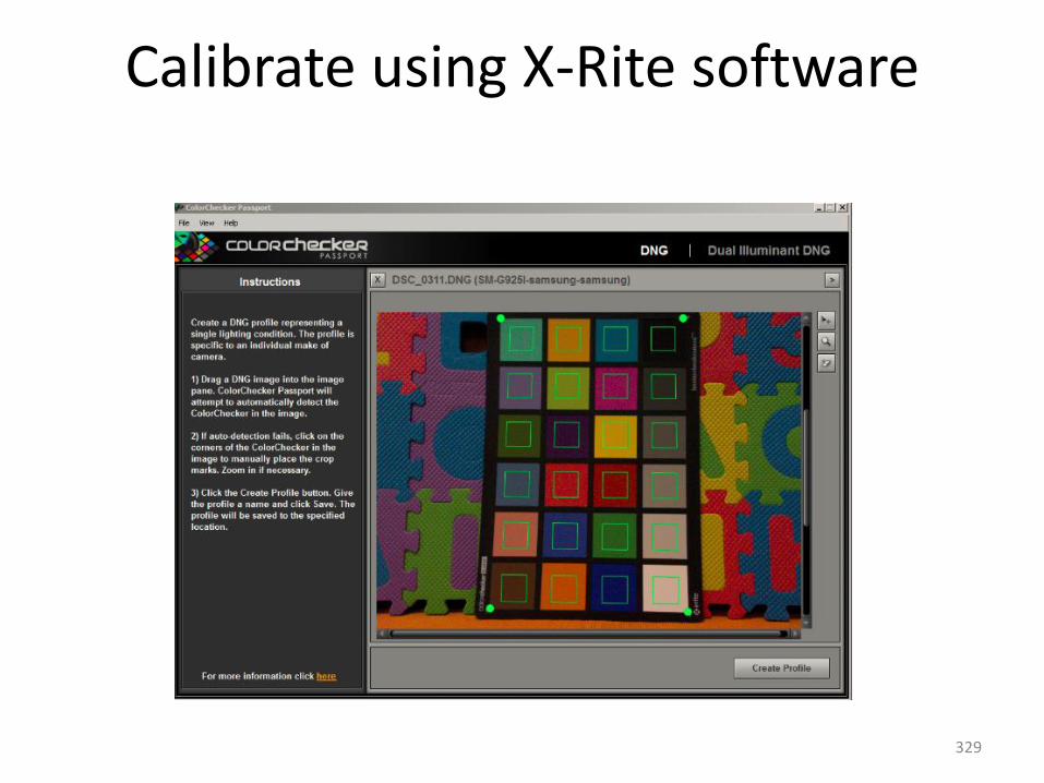
Calibrate using X-Rite software
329
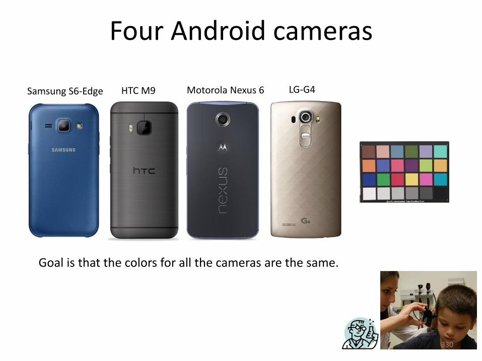
Four Android cameras
Samsung S6-Edge HTC M9 Motorola Nexus 6 LG-G4
Goal is that the colors for all the cameras are the same.
330
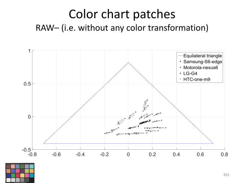
Color chart patchesRAW– (i.e. without any color transformation)
331

Color chart patchesRAW + white balanced and CST from the camera
332
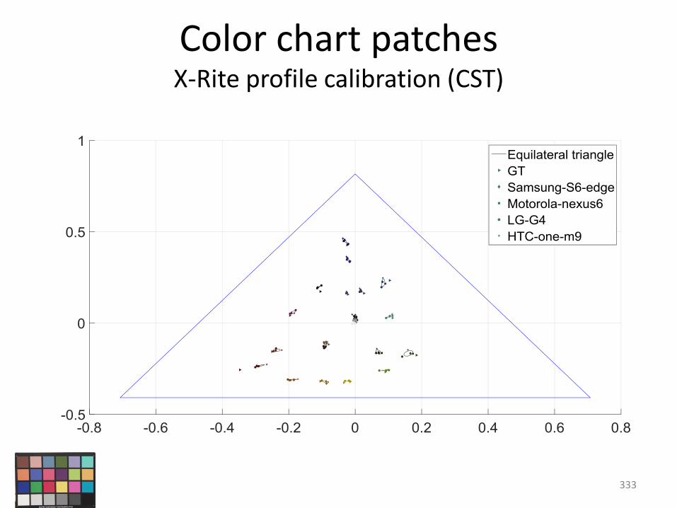
Color chart patchesX-Rite profile calibration (CST)
333
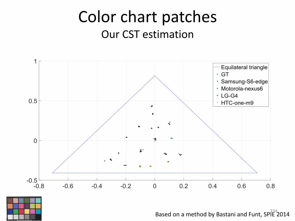
Color chart patchesOur CST estimation
Based on a method by Bastani and Funt, SPIE 2014334
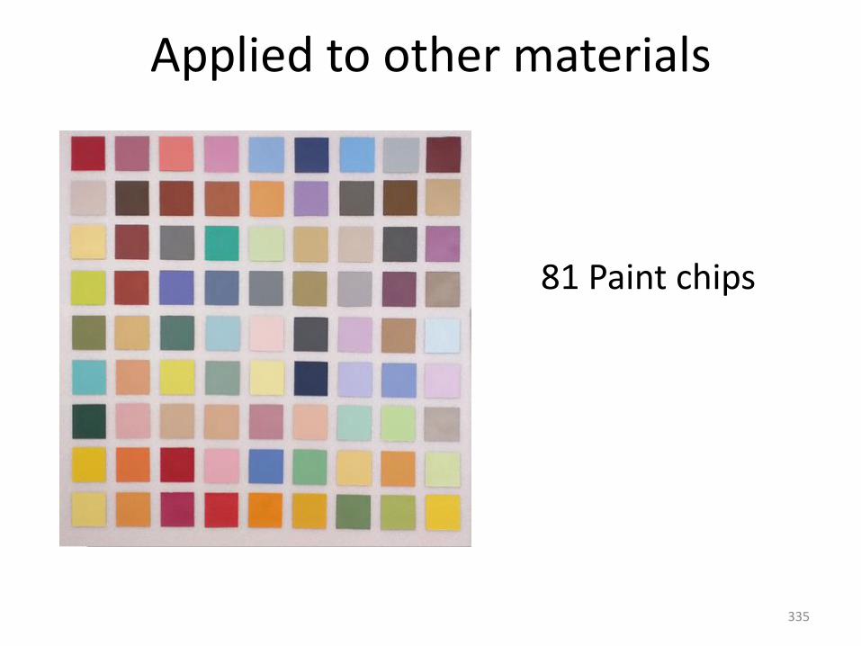
Applied to other materials
81 Paint chips
335

Additional materialsRAW– (i.e. without any color transformation)
336
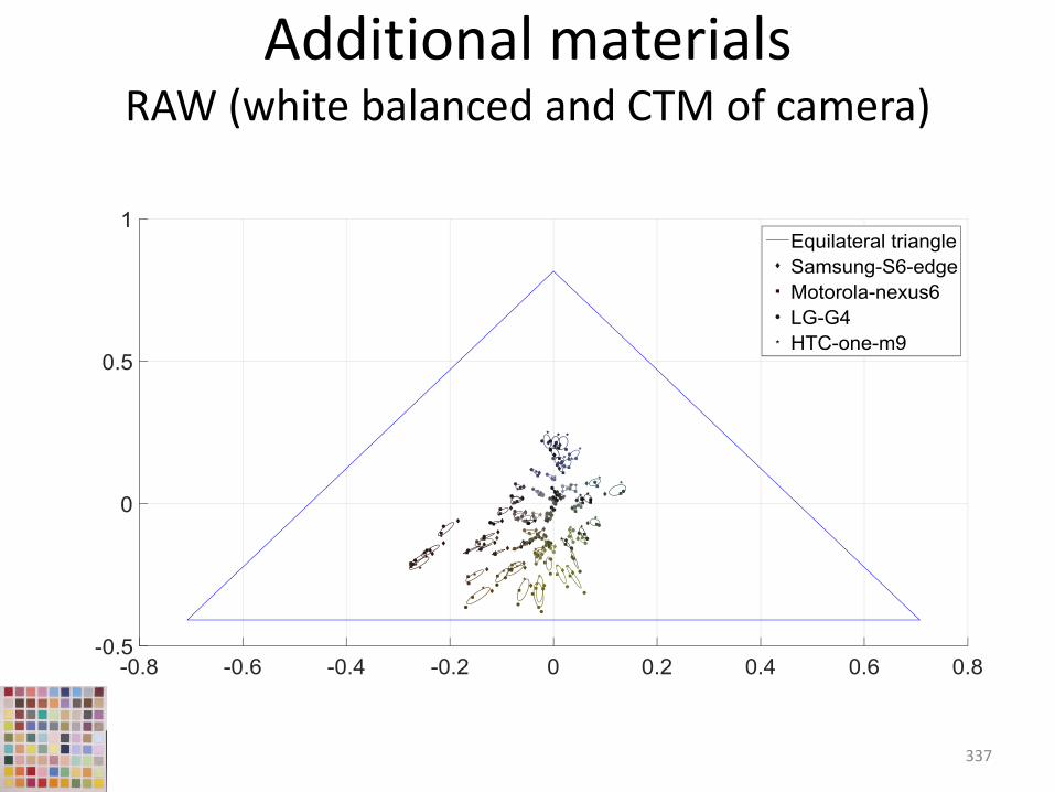
Additional materialsRAW (white balanced and CTM of camera)
337

Additional materialsX-rite Profile
338

Additional materialsOur CST estimation
339

True sRGB Example
sRGB
White Balance
Color Space Conversion
Hue/Sat Map Application
Reading RAW Image
Black Light Subtraction
Linearization
Lens CorrectionDemosaicing
Exposure Curve Application
Look Table Application
Tone Curve Application
Final Color Space Conversion
Gamma Curve Application
Noise Reduction
1 3 4
57
2
8 9 10
6
11
340

True sRGB vs. camera RGB
“True sRGB” Camera sRGB
341
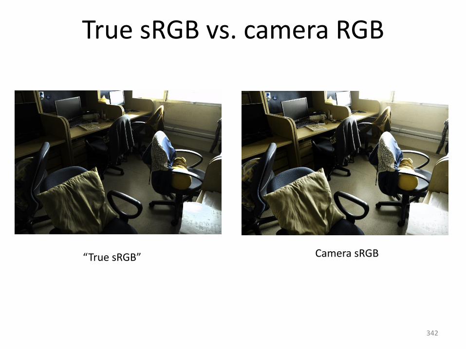
True sRGB vs. camera RGB
“True sRGB” Camera sRGB
342
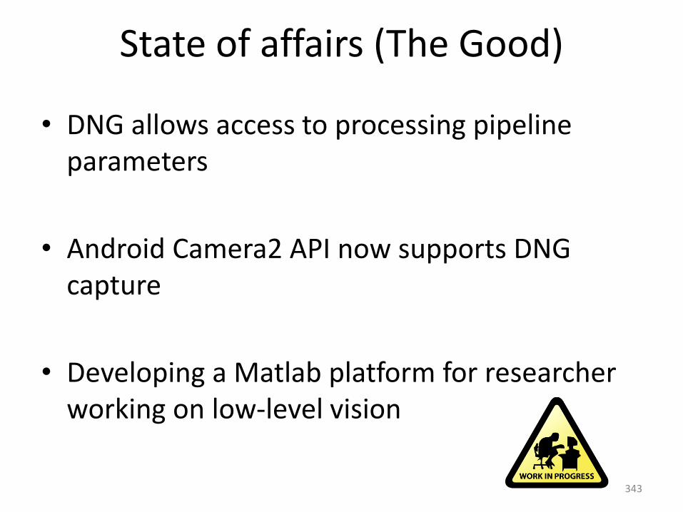
State of affairs (The Good)
• DNG allows access to processing pipeline parameters
• Android Camera2 API now supports DNG capture
• Developing a Matlab platform for researcher working on low-level vision
343
Concluding remarks
• Your camera performs a great deal of processing
• RAW – Represents relatively unprocessed sensor response
– Does not represent CIE XYZ
– Transform to CIE XYZ is not readily available
– There is no standard RAW!
• sRGB– Is defined with respect to CIE XYZ
– However, incoming radiant energy (SPDs) to sRGB is not standardize (otherwise all camera images would look the same)
344

Concluding remarks
• Our experiments found
– Mapping from RAW to sRGB changes for different picture styles (portrait, landscape, vivid, standard, etc. . )
– Picture styles can be modeled with a 3D function + tone-map
– White-balance (so far) seems independent of picture styles
345
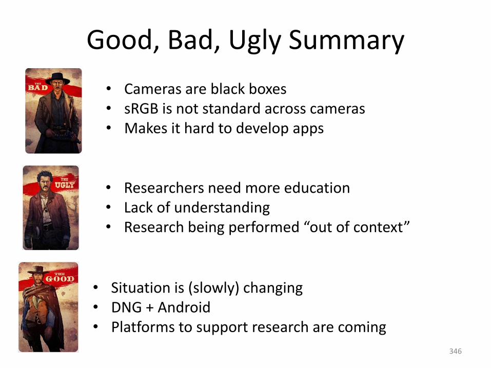
• Cameras are black boxes• sRGB is not standard across cameras• Makes it hard to develop apps
• Researchers need more education• Lack of understanding• Research being performed “out of context”
• Situation is (slowly) changing• DNG + Android• Platforms to support research are coming
Good, Bad, Ugly Summary
346
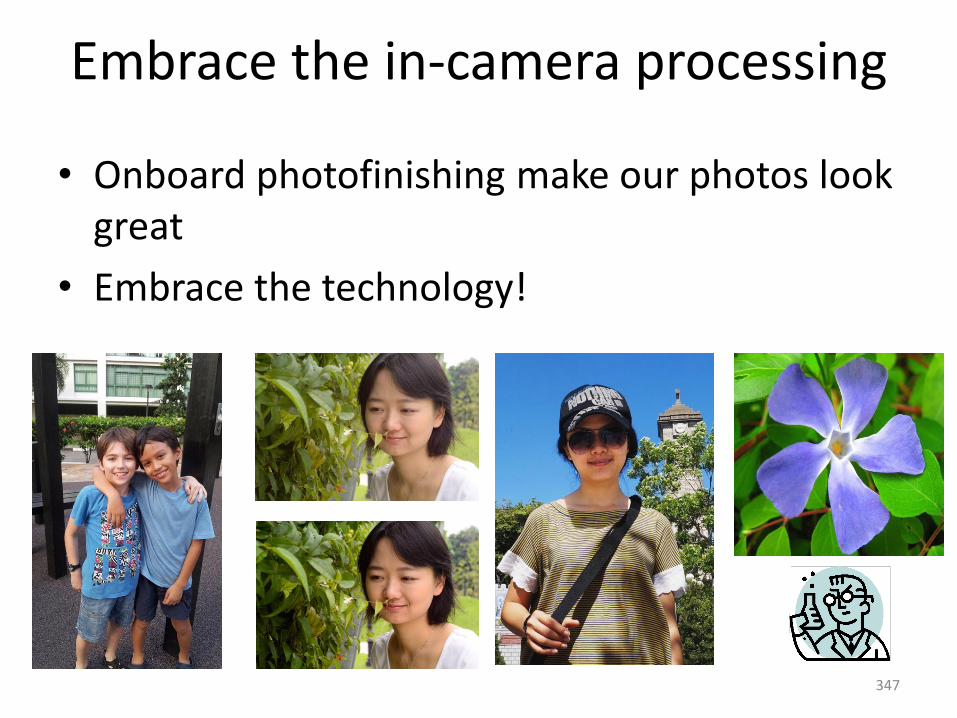
Embrace the in-camera processing
• Onboard photofinishing make our photos look great
• Embrace the technology!
347
Thank you for attending
Special thanks to my students and colleagues for contributing images, code,and materials to this tutorial.
Li Yu Hakki Karaimer Rang Nguyen Cheng Dongliang
348
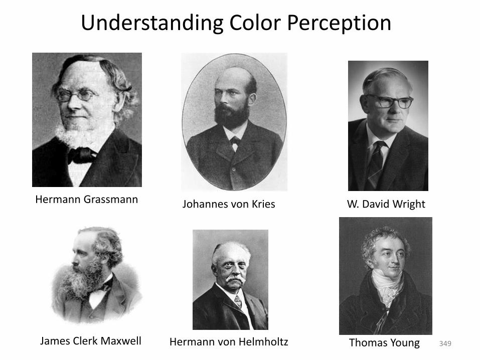
Hermann Grassmann Johannes von Kries W. David Wright
James Clerk Maxwell Hermann von Helmholtz Thomas Young
Understanding Color Perception
349
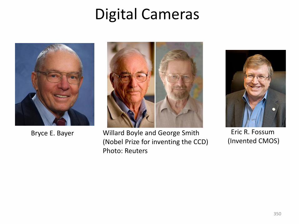
Bryce E. Bayer Willard Boyle and George Smith(Nobel Prize for inventing the CCD)Photo: Reuters
Eric R. Fossum(Invented CMOS)
Digital Cameras
350
And of course
“The Standard Observers”
351
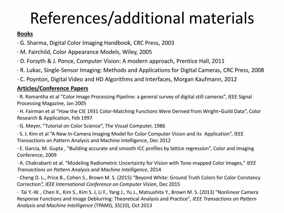
References/additional materialsBooks
∙ G. Sharma, Digital Color Imaging Handbook, CRC Press, 2003
∙ M. Fairchild, Color Appearance Models, Wiley, 2005
∙ D. Forsyth & J. Ponce, Computer Vision: A modern approach, Prentice Hall, 2011
∙ R. Lukac, Single-Sensor Imaging: Methods and Applications for Digital Cameras, CRC Press, 2008
∙ C. Poynton, Digital Video and HD Algorithms and Interfaces, Morgan Kaufmann, 2012
Articles/Conference Papers
∙ R. Ramantha et al “Color Image Processing Pipeline: a general survey of digital still cameras”, IEEE Signal Processing Magazine, Jan 2005
∙ H. Fairman et al “How the CIE 1931 Color-Matching Functions Were Derived from Wright–Guild Data”, Color Research & Application, Feb 1997
∙ G. Meyer, “Tutorial on Color Science”, The Visual Computer, 1986
∙ S. J. Kim et al “A New In-Camera Imaging Model for Color Computer Vision and its Application”, IEEE Transactions on Pattern Analysis and Machine Intelligence, Dec 2012
∙ E. Garcia, M. Gupta , “Building accurate and smooth ICC profiles by lattice regression”, Color and Imaging Conference, 2009
∙ A. Chakrabarti et al. "Modeling Radiometric Uncertainty for Vision with Tone-mapped Color Images," IEEE Transactions on Pattern Analysis and Machine Intelligence, 2014
∙ Cheng D. L., Price B., Cohen S., Brown M. S. (2015) “Beyond White: Ground Truth Colors for Color Constancy Correction”, IEEE International Conference on Computer Vision, Dec 2015
∙ Tai Y.-W. , Chen X., Kim S., Kim S. J, Li F., Yang J., Yu J., Matsushita Y., Brown M. S. (2013) "Nonlinear Camera Response Functions and Image Deblurring: Theoretical Analysis and Practice", IEEE Transactions on Pattern Analysis and Machine Intelligence (TPAMI), 35(10), Oct 2013
References/additional materials
Websites/Online ResourcesICC – ISO 22028 (2012) Document
Photo Tech Edu Series Jan 2007 (Google)
Available on youtube
Richard Lyon: Digital Camera Image Processing Pipelines
http://www.photo-mark.com
Mark Meyer Photography
Professional photography blog with nice tie-ins to color from a photographers point of view
http://dougkerr.net
Doug Kerr postings
A large collection of self-published articles on various aspects of imaging in an “accessible language” to most readers
353

Acknowledgements
This work was supported in part by generous gifts from:
• Adobe Research
• Google Research (Faculty Award 2015)
354


