Embed Size (px)
Citation preview
Integrative bioinformatics pipeline for
genome-wide association studies in neuropsychiatry
and the subsequent application
in Autism Spectrum Disorder cohorts
Dissertation
zur Erlangung des Doktorgrades
der Naturwissenschaften
im Fach Bioinformatik
vorgelegt beim Fachbereich Mathematik und Informatik
der Johann Wolfgang Goethe-Universität
in Frankfurt am Main
von
Afsheen Yousaf
aus Peshawar, Pakistan
Frankfurt (2019)
(D30)


vom Fachbereich Mathematik und Informatik der
Johann Wolfgang Goethe-Universität als Dissertation angenommen.
Dekan: Prof. Dr.-Ing. Lars Hedrich
1. Gutachter: Prof. Dr. Ina Koch
2. Gutachter: Prof. Dr. Christine M. Freitag
Datum der Disputation:


Dissertation Afsheen Yousaf Acknowledgments
Dissertation Afsheen Yousaf Table of contents
Table of contents
I. List of figures ......................................................................................................................... I
II. List of tables .......................................................................................................................... I
III. List of abbreviations ............................................................................................................. II
IV. List of genes ....................................................................................................................... IV
V. Preface...............................................................................................................................VII
VI. Zusammenfassung .............................................................................................................. IX
VII. Abstract .......................................................................................................................... XVII
1. Introduction ......................................................................................................................... 1
1.1. Motivation and structure of the thesis ..................................................................................................... 1 1.2. Genetic concepts ....................................................................................................................................... 2 1.3. Types of data in genetic studies ................................................................................................................ 4 1.4. ASD ............................................................................................................................................................ 8 1.5. Genetic studies designs ........................................................................................................................... 10 1.6. ASD data .................................................................................................................................................. 18 1.7. Data analysis............................................................................................................................................ 20 1.8. Aims of the study .................................................................................................................................... 26
2. Materials and methods ....................................................................................................... 29
2.1. ASD quantitative data ............................................................................................................................. 29 2.2. SNP genotype data .................................................................................................................................. 30
I. Preliminary data analysis of phenotype data ........................................................................... 30
2.3. Quality assurance of ADI-R data .............................................................................................................. 30 2.4. Phenotype imputation of missing ADI-R data ......................................................................................... 31 2.5. Identifying ADI-R subdomains ................................................................................................................. 32
II. The MAGNET tool: Implemented methods .............................................................................. 37
2.6. QC ............................................................................................................................................................ 37 2.7. Genotype imputation .............................................................................................................................. 44 2.8. GWAS ...................................................................................................................................................... 49 2.9. Gene-based analysis ................................................................................................................................ 51 2.10. Gene Ontology (GO) analysis .................................................................................................................. 52 2.11. Brain enrichment analysis ....................................................................................................................... 54
III. Additional data analysis ..................................................................................................... 55
2.12. Genetic correlation.................................................................................................................................. 55 2.13. SNP-based heritability analysis ............................................................................................................... 56 2.14. Polygenic risk scores (PRS) ...................................................................................................................... 57
3. Results and Discussion ........................................................................................................ 59
I. Preliminary analysis of phenotype data ................................................................................... 59
3.1. Phenotype imputation ............................................................................................................................ 59
II. (a) The MAGNET tool: Methodological results ......................................................................... 64
3.2. MAGNET implementation and architecture ............................................................................................ 64 3.3. MAGNET-lite ............................................................................................................................................ 78 3.4. Discussion ................................................................................................................................................ 78

Dissertation Afsheen Yousaf Table of contents
II. (b) The MAGNET tool: Biological results .................................................................................. 81
3.5. Quality check of genotype data ............................................................................................................... 81 3.6. Imputation of missing genotype data ...................................................................................................... 82 3.7. GWAS ....................................................................................................................................................... 83 3.8. Gene and pathway analysis ..................................................................................................................... 86 3.9. GO-term analysis...................................................................................................................................... 88 3.10. KEGG pathway analysis ............................................................................................................................ 88 3.11. Brain enrichment analysis ........................................................................................................................ 89
III. Additional data analysis ........................................................................................................ 96
3.12. Genetic heritability of ASD phenotypes ................................................................................................... 96 3.13. Correlation among ASD phenotypes ........................................................................................................ 97 3.14. PRS for ASD phenotypes .......................................................................................................................... 97 3.15. SNPs and genes overlap among the subdomains .................................................................................... 99 3.16. Discussion .............................................................................................................................................. 101
4. Conclusion and outlook .................................................................................................... 111
5. Appendix .......................................................................................................................... 115
5.1. Genetic terminologies ............................................................................................................................ 115 5.2. Genotype file formats ............................................................................................................................ 117 5.3. Statistical terms ..................................................................................................................................... 119 5.4. Supplementary figure ............................................................................................................................ 120
6. References ....................................................................................................................... 127
7. Curriculum vitae ............................................................................................................... 141
Dissertation Afsheen Yousaf List of figures and tables
I
I. List of figures
Figure 1 Allele frequency versus disease penetrance at different effect sizes .......................................... 3
Figure 2 Genotype imputation ................................................................................................................. 23
Figure 3 Minimac3 workflow using state-space reduction ...................................................................... 49
Figure 4 Scree plot of the AGP cohort ..................................................................................................... 60
Figure 5 PCA based subdomains of the 28 ADI-R items ........................................................................... 61
Figure 6 MAGNET workflow ..................................................................................................................... 64
Figure 7 General architecture of MAGNET .............................................................................................. 66
Figure 8 Quality check plots of IQ trait in German cohort ....................................................................... 69
Figure 9 MDS plot of the first two dimensions ........................................................................................ 81
Figure 10 Manhattan plots of the six subdomains from comb. cohort and IQ from the German cohort 85
Figure 11 Gene Ontology (GO) analysis ................................................................................................... 90
Figure 12 KEGG pathway analysis ............................................................................................................ 92
Figure 13 Expression profiles of associated brain gene modules ............................................................ 94
Figure 14 Heritability estimates ............................................................................................................... 96
Figure 15 Heatmaps illustrating the (a) phenotypic and (b) genetic corr. among ASD subdomains ....... 97
Figure 16 Polygenic risk score analysis .................................................................................................... 98
Figure 17 Overlap of significant findings................................................................................................ 100
II. List of tables
Table 1 Software used in MAGNET .......................................................................................................... 37
Table 2 Sample adequacy tests. ............................................................................................................... 59
Table 3 Factor loadings in AGP data set ................................................................................................... 62
Table 4 Confirmatory factor analysis in the German cohort ................................................................... 63
Table 5 Descriptive statistics .................................................................................................................... 63
Table 6 Computational requirements for MAGNET ................................................................................. 66
Table 7 Comparison with state-of-the-art Imputation frameworks. ....................................................... 77
Table 8 Genome-wide hits in combined, AGP and German cohort ......................................................... 84
Table 9 Significant genes in both cohorts from MAGMA analysis ........................................................... 87

Dissertation Afsheen Yousaf List of abbreviations
II
III. List of abbreviations
ADHD Attention deficit hyperactivity disorder ADI-R Autism Diagnostic Interview-Revised ADOS Autism Diagnostic Observation Schedule AGP Autism Genome Project AGRE Autism Genetic Resource Exchange API Application Program Interface ASC Autism Sequencing Consortium ASD Autism Spectrum Disorders BD Bipolar Disorder cDNA complementary Deoxyribonucleic Acid CFI Comparative Fit Index CI Confidence Interval CNV Copy number variant DAVID Database for Annotation, Visualization and Integrated Discovery Df Degree of freedom DFC Dorsolateral prefrontal cortex DNA Deoxyribonucleic acid DSM-IV Diagnostic and Statistical Manual of Mental Disorders, 4th Edition DZ Dizygotic twins EFA Exploratory Factor Analysis eQTL Expression quantitative trait loci FDR False Discovery Rate GO Gene Ontology GRCh37 Genome Reference Consortium Human build 37 grm genetic relationship matrix GSEA Gene set enrichment analysis GWAS Genome-wide association studies GUI Graphical User Interface Hs Homosapiens ICD International Statistical Classification of Diseases and Related Health Problems IPA Ingenuity Pathway Analysis IPC Inferior parietal cortex IQ Intelligence Quotient JA Joint attention kb kilobases KEGG Kyoto Encyclopedia of Genes and Genomes KMO Kaiser Maier Olkin KO Knockout LD Linkage Disequilibrium LOD Logarithm of odds LTD Long Term Depression LTP Long Term Potentiation MAGMA Multi-marker Analysis of GenoMic Annotation MAGNET MApping the Genetics of Neuropsychological Traits to molecular NETworks of
human brain MAF Minor Allele Frequency MCQs Multiple-choice questions MI Multiple imputation MDS Multidimensional Scaling MZ Monozygotic NCBI National Center for Biotechnology Information OFC orbito frontal cortex
Dissertation Afsheen Yousaf List of abbreviations
III
ORA Over-representation analysis PCA Principal components analysis pcw post-conceptional weeks PDD-NOS Pervasive developmental disorder-not otherwise specified PGC Psychiatric Genomics Consortium pmm predictive mean matching PRS Polygenic risk scores QC Quality Check QQ Quantile-quantile qGWAS quantitative genome-wide association study RB Repetitive sensory motor behavior RMSEA Root Mean Square Error Approximation RNA Ribonucleic acid RNA-Seq Ribonucleic acid- sequencing SNP Single Nucleotide Polymorphism SNV Single Nucleotide Variants SRMR Standardized Root Mean Square Residual STC Superior temporal cortex SRS Social Responsiveness Scale SZ Schizophrenia TDT Transmission-Disequilibrium Test TLI Tucker Lewis Index VCF Variant calling file VEGAS2 Versatile Gene-based Association Study 2
Dissertation Afsheen Yousaf List of genes
IV
IV. List of genes
ADCY2 Adenylate Cyclase 2 ADCY5 Adenylate Cyclase 5 ASTN2 Astrotactin 2 BIN1 Bridging Integrator 1 C8ORFK32 Family With Sequence Similarity 135 Member B CALCOCO2 Calcium Binding And Coiled-Coil Domain 2 CLIP2 CAP-Gly Domain Containing Linker Protein 2 CDH9 Cadherin 9 CDH10 Cadherin 10 CECR2 Cat Eye Syndrome Chromosome Region, Candidate 2 CMIP C-Maf Inducing Protein CNTNAP2 Contactin-associated protein-like 2 CNTN4 Contactin 4 CNTN5 Contactin 5 COBLL1 Cordon-Bleu WH2 Repeat Protein Like 1 CX3CR1 C-X3-C Motif Chemokine Receptor 1 DAGLA Diacylglycerol Lipase Alpha DDX53 DEAD-Box Helicase 53 DLGAP2 DLG Associated Protein 2 DLX3 Distal-Less Homeobox 3 ENPP3 Ectonucleotide Pyrophosphatase ERBB4 Erb-B2 Receptor Tyrosine Kinase 4 FER FER Tyrosine Kinase FTL Ferritin Light Chain GABRB3 Gamma-aminobutyric acid type A receptor beta3 subunit GNAO1 G Protein Subunit Alpha O1 GNAS Guanine Nucleotide Binding Protein (G Protein) GNG2 G Protein Subunit Gamma 2 GYS1 Glycogen Synthase 1 HTT Huntingtin ICA1 Islet Cell Autoantigen 1 IL20 Interleukin 20 KCND2 Potassium Voltage-Gated Channel Subfamily D Member 2 LHB Luteinizing Hormone Beta Polypeptide MACROD2 Mono-ADP Ribosylhydrolase 2 MCF2L MCF2 Cell Line Derived Transforming Sequence Like MNS1 Meiosis Specific Nuclear Structural 1 MPN2 Serine Protease 38 NELL1 Neural EGFL Like 1 NLGN1 Neuroligin 1 NLGN4 Neuroligin 4 NLRP3 NLR Family Pyrin Domain Containing 3 NOS2A Nitric Oxide Synthase 2 NRXN1 Neurexin 1 NSUN5 NOP2/Sun RNA Methyltransferase 5 NTRK3 Neurotrophic Receptor Tyrosine Kinase 3 PANX1 Pannexin 1 PANX2 Pannexin 2 PARK2 Parkin RBR E3 Ubiquitin Protein Ligase PATJ PALS1-Associated Tight Junction Protein PGLYRP2 Peptidoglycan Recognition Protein 2 PHB Prohibitin PLCB2 Phospholipase C Beta 2
Dissertation Afsheen Yousaf List of genes
V
PPM1N Probable Protein Phosphatase 1N PTCHD1 Patched Domain Containing 1 QPRT Quinolinate Phosphoribosyltransferase RGS10 Regulator Of G Protein Signaling 10 RNPS1 RNA Binding Protein With Serine Rich Domain 1 RORA Retinoic acid-related orphan receptor alpha S100A3 S100 calcium-binding protein A3 S100A4 S100 calcium-binding protein A4 S100A5 S100 calcium-binding protein A5 SCN5A Sodium Voltage-Gated Channel Alpha Subunit 5 SCN8A Sodium Voltage-Gated Channel Alpha Subunit 8 SDK1 Sidekick Cell Adhesion Molecule 1 SEMA5A Semaphorin 5A SHANK2 SH3 And Multiple Ankyrin Repeat Domains 2 SLC22A18AS Solute Carrier Family 22 Member 18 Antisense SLC25A12 Solute Carrier Family 25 Member 12 SLC26A5 Solute Carrier Family 26 Member 5 SLC35B1 Solute Carrier Family 35 Member B1 SYNGAP1 Synaptic Ras GTPase Activating Protein 1 TAS2R1 Taste 2 Receptor Member 1 THRA Thyroid Hormone Receptor Alpha TM4SF4 Transmembrane 4 L Six Family Member 4 TTC17 Tetratricopeptide Repeat Domain 17 TYROPB TYRO Protein Tyrosine Kinase Binding Protein

Dissertation Afsheen Yousaf List of genes
VI
Dissertation Afsheen Yousaf Preface
VII
V. Preface
The work presented in this thesis has been performed at two Departments of the Goethe University
Frankfurt, which is the “Molecular Bioinformatics” (Prof. Dr. Ina Koch) and “Department of Child and
Adolescent Psychiatry, Psychosomatics and Psychotherapy” (Prof. Dr. Christine M. Freitag). In addition,
Dr. Andreas G. Chiocchetti supervised my thesis at the Molecular Genetics Lab of the Department of
Child and Adolescent Psychiatry, Psychosomatics and Psychotherapy.
In this work, I present the development and implementation of an integrative bioinformatics pipeline
designed for genetic analyses of neuropsychiatric traits. The aim is to identify the associated genetic
variants, underlying biological pathways of the traits, and to map the genetic association to the
developing human brain. The pipeline is called “MAGNET” (MApping the Genetics of neuropsychiatric
traits to molecular NETworks of the human brain). MAGNET was developed adhering to the state-of-
the-art guidelines for genome-wide single nucleotide polymorphism (SNP) imputation, quality control
and genome-wide association studies (GWAS).
MAGNET has been already used successfully to analyse data in different studies that have already been
published. This includes a meta-analysis study across five different European populations analysing
variants associated with ASD candidate genes. This study entitled “Lack of replication of previous
autism spectrum disorder GWAS hits in European populations” was published in Autism Research by
Dr. Bàrbara Torrico and Dr. Claudio Toma where I and Dr. Andreas G. Chiocchetti helped to provide the
respective variants by using MAGNET for imputation in large ASD datasets 1.
In another study, we investigated the genetic variants of the glutamatergic system in ASD with high
and low intellectual abilities. This work was published in the Journal of Neurotransmission as “Common
functional variants of the glutamatergic system in Autism spectrum disorder with high and low
intellectual abilities”. I performed the data analysis, mainly using the MAGNET pipeline along with
other algorithms to identify genes associated with high and low Intelligence Quotient (IQ) cohorts. The

Dissertation Afsheen Yousaf Preface
VIII
concept and design of this work were developed by Dr. Andreas G. Chiocchetti and Prof. Christine M.
Freitag 2.
Parts of MAGNET have also been implemented in the work by Dr. Denise Haslinger and Dr. Andreas G.
Chiocchetti, i.e. “Loss of the Chr16p11.2 ASD candidate gene QPRT leads to aberrant neuronal
differentiation in the SH-SY5Y neuronal cell model”. There, we applied MAGNET on a transcriptome
dataset to identify the gene networks of brain development within genes significantly differentially
regulated upon knock out (KO) of the gene QPRT 3.
A paper regarding the detailed features and implementation of MAGNET on IQ trait in a cohort is
available as a preprint at bioarXiv. This work helped to identify novel candidate genes associated with
IQ and also identified the genes already known in association with IQ. Thus, the study provided a
successful proof of concept for MAGNET. The design and analysis were supported by Dr. Andreas G.
Chiocchetti and supervised by Prof. Ina Koch.
The main work related to MAGNET has been submitted to Translational Psychiatry. The publication
focuses on the results generated using MAGNET and important novel findings gathered with respect to
ASD quantitative phenotypes. I analysed two large ASD cohorts by using MAGNET and wrote the
manuscript. The concept and design of the project were supported by Dr. Andreas G: Chiocchetti and
Prof. Christine M. Freitag. Prof as well as both the co-authors supported in manuscript preparation. Ina
Koch supported data analysis and manuscript revision.
In summary, the presented pipeline has been already implemented in three publications 1–3 (see
Publication list). The pipeline is available as a preprint at bioarXiv and the work related to the
implementation of the pipeline on ASD cohorts has been submitted to the journal of Translational
Psychiatry. This thesis focuses on the work presented in the following two publications:
I. MApping the Genetics of neuropsychiatric traits to molecular NETworks of the human brain
(preprint bioRxiv 10.1101/336776).
II. Quantitative genome-wide association study of six phenotypic subdomains identifies novel
genome-wide significant variants in Autism Spectrum Disorder (In review).

Dissertation Afsheen Yousaf Zusammenfassung
IX
VI. Zusammenfassung
Motivation
Neuropsychiatrische Erkrankungen sind komplexe Störungen mit hoher Heritabilität und
weitestgehend unaufgeklärten Pathomechanismen. Die klinische und genetische Heterogenität dieser
Erkrankungen stellt eine große Herausforderung für die Identifizierung von krankheitsbezogenen
Biomarkern dar. Neben signifikanten Fortschritten bei der Aufklärung der genetischen Grundlagen
dieser Erkrankungen bleiben die zugrunde liegenden Ursachen und biologischen Mechanismen
verborgen. Mit der Weiterentwicklung der Array-, Sequenzierungs- und Big-Data-Technologien werden
große Datenmengen von Einzelpersonen auf verschiedensten Plattformen und in verschiedensten
Datenstrukturen erzeugt. Es gibt allerdings nur wenige Bioinformatik-Tools, die diese Fülle von Daten
integrieren und verarbeiten können. Daher ist es notwendig, ein integratives bioinformatisches
Datenanalysetool zu entwickeln, welches diese Daten im Sinne eines Big-Data Ansatzes kombiniert, um
die zugrunde liegende Genetik besser zu verstehen und die Ergebnisse auf die humane
Gehirnentwicklung zu übertragen, mit dem Ziel die mit den jeweiligen Störungen verbundenen
Pathomechanismen aufzuklären.
Einleitung:
Diese Arbeit stellt eine Bioinformatik-Pipeline vor, welche Daten von verschiedenen Plattformen
implementiert, um ein grundlegendes Verständnis der genetischen Ätiologie eines
neuropsychiatrischen quantitativen/qualitativen Merkmals zu generieren. Innerhalb dieser Arbeit
werden zwei Aspekte behandelt: Einer ist die Entwicklung und der Aufbau einer Bioinformatik-Pipeline
namens MApping the Genetics of neuropsychiatric traits to the molecular NETworks of the human brain
(MAGNET). Der andere Teil zeigt die Implementierung und den Nutzen von MAGNET bei der Analyse
großer ASS-Kohorten (Autismus-Spektrum-Störungen).
Um biologische und klinische Daten verschiedener Plattformen zu integrieren, sind effiziente
Bioinformatik-Werkzeuge erforderlich, von denen derzeit nur wenige verfügbar sind. In dieser Arbeit

Dissertation Afsheen Yousaf Zusammenfassung
X
präsentieren wir eine Bioinformatik-Pipeline, die Genotyp-, Verhaltensmerkmal- und
Genexpressionsdaten kombiniert. Ziel ist hierbei die genetischen Assoziationen eines
neuropsychiatrischen Merkmals mit der genetischen Regulation der Gehirnentwicklung in Relation zu
setzen, um so ein umfassendes Verständnis zu erhalten, das über die Identifikation von genetischen
Risikofaktoren hinausgeht. MAGNET ist ein frei verfügbares command-line Tool, das innerhalb eines
Frameworks Datenintegrationsansätze auf der Grundlage modernster Algorithmen und Software
implementiert, um schließlich die Gene und Pfade zu identifizieren, die genetisch mit einem
spezifischen quantitativen aber auch qualitativen Merkmal verbunden sind. MAGNET bietet einen
zentralen Vorteil gegenüber den bestehenden Tools, da es neben der umfassenden genetischen
Analyse die Datenverarbeitung und die Daten-Parsing-Schritte automatisiert, die für die
Kommunikation zwischen den verschiedenen APIs (Application Program Interface) notwendig sind.
Dabei unterstützt MAGNET genau die Zwischenschritte der Datenverarbeitung, die von Forschern
benötigt werden, um von einer Analyse zur nächsten zu gelangen. Darüber hinaus können Anwender je
nach Größe des Datensatzes innerhalb weniger Tage essentielle Informationen über ihr gewünschtes
Merkmal ableiten wie genetische Assoziationen oder die Kartierung der zugehörigen Gene auf die
Entwicklung des menschlichen Gehirns mit Transkriptomdaten von 16 verschiedenen Gehirnregionen
von der 5. postkonzeptionellen Woche bis zum Alter von über 40 Jahren.
MAGNET kann für jede neuropsychiatrische Störung, für die häufige Varianten ätiologisch relevant
sind, verwendet werden. MAGNET verarbeitet SNP- (Single Nucleotide
Polymorphism/Einzelnukleotidpolymorphismus) basierte Genotypdaten und setzt diese in Korrelation
mit einem quantitativen bzw qualitativen Merkmal. Speziell neuropsychiatrische Erkrankungen sind
komplexe und heterogene Störungen, welche zwar eine hohe Heritabilität aufweisen, aber deren
Pathomechanismen trotz Fortschritten in der DNA-Analyse noch weitgehend unklar sind. Zu diesen
Störungen gehören ASS (Autismus-Spektrum-Störung), ADHS (Aufmerksamkeitsdefizit-
Hyperaktivitätsstörung), BS (Bipolare Störung) und SZ (Schizophrenie). Von betroffenen Personen
stehen große Mengen an Genotyp- und Verhaltensdaten zur Verfügung. Basierend auf diesen Daten

Dissertation Afsheen Yousaf Zusammenfassung
XI
können wir signifikante genetische Varianten sowie Gene identifizieren, die mit den Verhaltensdaten
oder klinischen Daten assoziiert sind. Darüber hinaus kann der Vergleich dieser assoziierten Gene mit
Genexpressionsdaten des menschlichen Gehirns Schlüsselregionen und Zeitpunkte identifizieren,
welche für verschiedene neuronale Entwicklungsphasen des menschlichen Gehirns eine Rolle spielen.
Unser Ziel war es also, ein bioinformatisches Werkzeug zu entwickeln, das es Forschern erleichtert, die
zugrundeliegenden genetischen Aspekte ihres gewünschten Merkmals in einer Pipeline zu sammeln,
indem Daten aus verschiedenen Ebenen kombiniert werden. Auf diese Weise können die
Pathomechanismen neuropsychiatrischer Störungen besser identifiziert werden.
Im zweiten Teil, dem Proof of Concept, haben wir MAGNET auf zwei ASD-Kohorten implementiert.
Diese Arbeit konzentriert sich auf die Auswertung von Daten, welche in einer Stichprobe von Patienten
mit ASS erhoben wurden. ASS ist eine Gruppe von psychiatrischen Erkrankungen, denen eine
neuronale Entwicklungsstörung zugrunde liegt. Klinisch wird die Psychopathologie von ASS wie folgt
charakterisiert: A) Einschränkungen in der sozialen Interaktion und Kommunikation sowie B)
eingeschränktes, repetitives Verhalten. Die Ätiologie der Erkrankungen ist aufgrund ihrer heterogenen
klinischen und genetischen Eigenschaften äußerst komplex. Daher wurden bisher keine zuverlässigen
Biomarker identifiziert. Die Diagnose basiert aktuell ausschließlich auf der Beschreibung des Verhaltens
durch die Eltern sowie auf der direkten Verhaltensbeobachtung des Kindes. Ziel dieses Teils der Studie
war es, die genetische Architektur von ASS unter Berücksichtigung der beiden oben genannten ASS-
Diagnostikgebiete zu charakterisieren. Außerdem wurde untersucht, ob diese Bereiche genetisch
verknüpft oder unabhängig voneinander sind. Darüber hinaus haben wir uns mit der Frage beschäftigt,
ob diese Merkmale das genetische Risiko (polygenic risk score/PRS) mit der kategorischen Diagnose
von ASS teilen und wie viel von der phänotypischen Varianz dieser Merkmale durch die zugrunde
liegende Genetik erklärt werden kann.
Methoden:
Im ersten Teil wurden vorbereitende Analysen zur Aufbereitung der Phänotpydaten durchgeführt. Es
wurden folgende Datensätze eingeschlossen: Patienten mit ASS aus dem Autism-Genome-Project
Dissertation Afsheen Yousaf Zusammenfassung
XII
(AGP, n=2 735) sowie eine deutsche Kohorte, bestehend aus Proben, welche in Frankfurt gesammelt
wurden (n=705). Ziel der Studie war es, die genetische Architektur von ASS unter Berücksichtigung der
beiden ASS-Diagnosebereiche Domäne A (soziale Interaktion und Kommunikation) und Domäne B
(repetitives, stereotypes Verhalten, sensorische Auffälligkeiten und Sonderinteressen) zu
charakterisieren.
Die verwendeten Phänotypdaten wurden mithilfe des Tools „Diagnostisches Interview für Autismus –
Revidiert“ (ADI-R) erhoben. Es beinhaltet 93 Items zur frühkindlichen Entwicklung, zu Spracherwerb
und möglichem Verlust von sprachlichen Fertigkeiten, verbalen und nonverbalen kommunikativen
Fähigkeiten, Spiel- und sozialem Interaktionsverhalten sowie stereotypen Interessen und Aktivitäten.
Wir haben 28 Items ausgewählt, welche zum einen für die diagnostischen Algorithmen aus ADI-R
notwendig sind, und zum anderen sowohl für verbale als auch für nonverbale Personen verfügbar
waren. Darüber hinaus wurden demografische Daten wie Alter, Geschlecht und IQ der betroffenen
Personen verwendet. Personen mit mehr als 10% fehlenden Phänotypinformationen nach
Qualitätskontrolle wurden ausgeschlossen. Anschließend wurde die Phänotypdaten-Imputation für die
28 Algorithmenelemente durchgeführt. Die korrekte Kodierung des ADI-R wurde zusätzlich überprüft.
Um die bekannte phänotypische Heterogenität zu reduzieren und die dimensionalen Eigenschaften als
Zielgröße für die Analyse genetischer Risikofaktoren für einen unterschiedlichen ASS-Schweregrad zu
definieren, wurde eine Hauptkomponentenanalyse für die einzelnen Items des ADI-R in der AGP-
Kohorte durchgeführt, um mögliche Komponenten/Subdomänen zu beschreiben. Im Anschluss wurde
in der deutschen Kohorte eine konfirmatorische Faktorenanalyse durchgeführt, um festzustellen, ob
die in der AGP-Kohorte erhaltenen Subdomänen in einer unabhängigen Kohorte repliziert werden
können.
Im zweiten Teil wurde MAGNET auf jede der ASS-Subdomänen als eine quantitative abhängige Variable
angewendet. Die Analyse-Pipeline MAGNET ist in fünf Hauptabschnitte unterteilt. Der erste Abschnitt
führt eine umfassende Qualitätsprüfung der Genotypdaten durch. Diese umfasst das Filtern fehlender
Genotypdaten über einem bestimmten Schwellenwert, die Überprüfung auf Geschlechtsunterschiede,
Dissertation Afsheen Yousaf Zusammenfassung
XIII
Kontaminations- und Inzuchtfehler sowie die Visualisierung der Populationsstratifikation. Nach der
Qualitätskontrolle der Genotypdaten werden im zweiten Abschnitt die fehlenden Genotypen anhand
eines Referenzdatensatzes imputiert. Im dritten Abschnitt wird die Assoziationsanalyse von Genotyp-
und einzelnen Merkmalsdaten mittels Regressionsanalyse durchgeführt, um assoziierte genetische
Varianten zu finden. Im vierten Abschnitt wird eine genbasierte Analyse durchgeführt, die alle
Varianten aus der Regressionsanalyse als Input übernimmt. Danach werden die genetischen Varianten
den entsprechenden Genen zugeordnet und signifikante Gene werden weiteren Analysen unterzogen.
Zusätzlich werden in diesem Abschnitt biologische Signalwege identifiziert, welche mit den
signifikanten Genen assoziiert sind. Im letzten Abschnitt werden bereits vorhandene
Genexpressionsdaten aus dem menschlichen Gehirn integriert (Kang et al.,2011). Diese Daten
beschreiben 29 verschiedene genetische neuronale Module mit einem spezifischen Expressionsmuster
zu verschiedenen Zeitpunkten (beginnend mit der 5. postkonzeptionellen Woche bis über 40 Jahre) in
16 verschiedenen Gehirnregionen. Die mit den unterschiedlichen Phänotypen assoziierten Gene
werden bezüglich ihrer Überlappungen mit den 29 Genexpressionsmodulen getestet. Für die
wichtigsten Gene werden Heatmaps der Expression aller Gene innerhalb des assoziierten Moduls
erstellt, sodass eine ätiologische Interpretation möglich wird.
Im dritten Teil dieser Arbeit wurden zusätzliche Analysen durchgeführt, um den Anteil der
phänotypischen Varianz zu bestimmen, der durch genetische Varianten (SNPs) für jede Subdomäne,
d.h. die SNP-basierte Heritabilität erklärt wird. Darüber hinaus wurde eine genetische
Korrelationsanalyse zwischen den Subdomänen durchgeführt, um festzustellen, ob Subdomänen, die
sich auf Domäne A beziehen, und die Subdomänen, die sich auf Domäne B beziehen, genetisch
verknüpft oder unabhängig voneinander sind. Am Ende wurde das polygenetische Risiko
berücksichtigt, welches zwischen ASS und den einzelnen Subdomänen überlappt.
Ergebnisse:
Die Analyse aus dem ersten Teil der Arbeit (Aufbereitung der Phänotypdaten) identifizierte sechs
aussagekräftige Komponenten in der AGP-Stichprobe, die jeweils ein quantitatives ASS-Merkmal oder
Dissertation Afsheen Yousaf Zusammenfassung
XIV
eine Subdomäne darstellen. Vier Subdomänen, nämlich "social interaction" (SI), "joint attention" (JA),
"peer interaction" (PI) und "non-verbal communication" (NVC) sind Subdomänen des Bereichs A
(soziale Interaktion und Kommunikation), die beiden weiteren Subdomänen "repetitive sensory-motor
behavior" (RB) und "restricted interests" (RI) gehören zu Bereich B (repetitives, stereotypes Verhalten,
sensorische Auffälligkeiten und Sonderinteressen). Die Subdomänen wurden in der zweiten, deutschen
ASS-Kohorten bestätigt.
Die Qualitätskontrolle und Imputation der fehlenden SNP-Genotypdaten in einzelnen Kohorten im
zweiten Teil (MAGNET Implmentierung) der Arbeit erfolgte automatisiert durch MAGNET. Im nächsten
Schritt wurden assoziierte Varianten für jede Subdomäne im kombinierten AGP und deutschen
Datensatz identifiziert und ihren jeweiligen Genen zugeordnet. Wir fanden acht genomweit signifikante
SNPs, sowie 292 nominal signifikante bekannte und neue ASS-Risikogene. Diese Gene wurden im
Anschluss über MAGNET biologischen Signalwegen und Gen-Ontologien zugeordnet. Die
zugrundeliegenden biologischen Mechanismen konvergierten zu neuronalen Übertragungs- und
Entwicklungsprozessen. Über einen erneuten Abgleich dieser Gene mit dem Transkriptom des sich
entwickelnden humanen Gehirns konnte über MAGNET herausgefunden werden, dass die
signifikanten, mit den Subdomänen assoziierten Gene zu bestimmten Zeitpunkten in Gehirnarealen
wie dem Hippocampus, der Amygdala und kortikalen Regionen exprimiert werden.
In der zusätzlichen Analyse im dritten Teil haben wir festgestellt, dass die kollektive SNP-basierte
Heritabilität, die durch einzelne Subdomänen erklärt wird, höher ist als die bekannte SNP-basierte
Heritabilität von ASS. Wir konnten außerdem zeigen, dass die Subdomänen NVC, SI und PI das
polygenetische Risiko teilen, während die Subdomänen von RB und RI genetisch unabhängig
voneinander scheinen. Darüber hinaus spiegelt die genetische Korrelation zwischen den Subdomänen
teilweise phänotypische Domänen von ASS wider.
Conclusio:
MAGNET ist ein frei verfügbares command line tool, das auf Github zugänglich ist
(https://github.com/SheenYo/MAGNET). MAGNET bietet eine effiziente Datenintegration der Big-Data-
Dissertation Afsheen Yousaf Zusammenfassung
XV
Analyse und bewältigt automatisches Datenparsing sowie parallele Berechnung und
Datenqualitätsprüfungen . Es führt gründliche Analysen durch, die von der Qualitätskontrolle der
Genotypdaten bis hin zur Visualisierung von Gennetzwerken und Genexpressionsmustern wichtiger
Gene reichen. MAGNET implementiert state-of-the-art Software, um assoziierte häufige genetische
Varianten und Gene sowie deren biologische Relevanz zu identifizieren, welche mit einem bestimmten
Merkmal assoziiert sind. Darüber hinaus können die Gene in Beziehung zum Transkriptom des sich
entwickelnden menschlichen Gehirns gesetzt werden. MAGNET wurde erfolgreich zur Optimierung
genomweiter Assoziationsstudien eingesetzt und hat sich im Bereich der ASS-Forschung bewährt. Die
vom ADI-R-Algorithmus abgeleiteten Subdomänen im Zusammenhang mit der sozialen Kommunikation
zeigen eine gemeinsame genetische Ätiologie im Gegensatz zu eingeschränkten und repetitiven
Verhaltensweisen. Die ASS-spezifischen PRS überschnitten sich nur teilweise, was auf eine zusätzliche
Rolle der spezifischen gemeinsamen Variation bei der Gestaltung der phänotypischen Expression von
ASS-Subdomänen hindeutet.

Dissertation Afsheen Yousaf Zusammenfassung
XVI
Dissertation Afsheen Yousaf Abstract
XVII
VII. Abstract
Motivation
Neuropsychiatric disorders are complex, highly heritable but incompletely understood disorders. The
clinical and genetic heterogeneity of these disorders poses a significant challenge to the identification
of disorder related biomarkers. Besides significant progress in unveiling the genetic basis of these
disorders, the underlying causes and biological mechanisms remain obscure. With the advancement in
the array, sequencing, and big data technologies, a huge amount of data is generated from individuals
across different platforms and in various data structures. But there is a paucity of bioinformatics tools
that can integrate this plethora of data. Therefore, there is a need to develop an integrative
bioinformatics data analysis tool that combines biological and clinical data from different data types to
better understand the underlying genetics. For example, identifying significant genetic variants as well
as genes that are associated with the behavioral data of these disorders. Moreover, integrating gene
expression data of the human brain can highlight these associated genes with respect to key regions
and time points that are altered during different neurodevelopmental stages of a human brain.
Introduction
This thesis presents a bioinformatics pipeline implementing data from different platforms to provide a
thorough understanding of the genetic etiology of a neuropsychiatric quantitative as well as a
qualitative trait of interest. Throughout the thesis, we present two aspects: one is the development
and architecture of the bioinformatics pipeline named MApping the Genetics of neuropsychiatric traits
to the molecular NETworks of the human brain (MAGNET). The other part demonstrates the
implementation and usefulness of MAGNET analysing large Autism Spectrum Disorder (ASD) cohorts.
MAGNET is a freely available command-line tool available on GitHub
(https://github.com/SheenYo/MAGNET). It is implemented within one framework using data
integration approaches based on state-of-the-art algorithms and software to ultimately identify the
genes and pathways genetically associated with a trait of interest. MAGNET provides an edge over the
Dissertation Afsheen Yousaf Abstract
XVIII
existing tools since it performs a comprehensive analysis taking care of the data handling and parsing
steps necessary to communicate between the different APIs (Application Program Interface). Thus, this
avoids the in-between data handling steps required by researchers to provide output from one analysis
to the next. Moreover, depending on the size of the dataset users can deduce important information
regarding their trait of interest within a time frame of a few days. Besides gaining insights into genetic
associations, one of the central features is the mapping of the associated genes onto developing
human brain implementing transcriptome data of 16 different brain regions starting from the 5th post-
conceptional week to over 40 years of age.
In the second part as proof of concept, we implemented MAGNET on two ASD cohorts. ASD is a group
of psychiatric disorders. Clinically, ASD is characterized by the following psychopathology: A)
limitations in social interaction and communication, and B) restricted, repetitive behavior. The etiology
of this disorder is extremely complex due to its heterogeneous clinical traits and genetics. Therefore, to
date, no reliable biomarkers are identified. Here, the aim is to characterize the genetic architecture of
ASD taking into account the two aforementioned ASD diagnostic domains. As well as to investigate if
these domains are genetically linked or independent of each other. Moreover, we addressed the
question if these traits share genetic risk with the categorical diagnosis of ASD and how much of the
phenotypic variance of these traits can be explained by the underlying genetics.
Methods
In the first part, preliminary analyses were performed which incorporated statistical data analysis
approaches. We included affected individuals from two ASD cohorts, i.e. the Autism Genome Project
(AGP) and a German cohort consisting of 2,735 and 705 families respectively. We used phenotype data
gathered from diagnostic interviews for Autism - Revised (ADI-R). Firstly, the quality of the phenotype
data was ensured. In order to reduce the known phenotypic heterogeneity and to define the
dimensional properties as a target for the analysis of genetic risk factors, a principal component
analysis was performed on the ADI-R data in the AGP cohort. Subsequently, a confirmatory factor
Dissertation Afsheen Yousaf Abstract
XIX
analysis was performed in the German cohort to determine whether the subdomains obtained in the
AGP cohort could be replicated in an independent cohort.
In the second part, MAGNET was applied to each of the ASD subdomains as a quantitative dependent
variable. MAGNET is divided into five main sections i.e. (1) quality check of the genotype data, (2)
imputation of missing genotype data, (3) association analysis of genotype and trait data, (4) gene-
based analysis, and (5) enrichment analysis using gene expression data from the human brain.
In the third part of this thesis, the proof of concept study was extended with additional analyses. These
analyses included determination of the SNP-based heritability for each subdomain. In addition, a
genetic correlation analysis between subdomains was performed to identify whether subdomains
related to ASD domains A and B are genetically linked or independent of each other. Finally, the
polygenic risk overlapping between ASD and each subdomain was considered.
Results
The preliminary analyses identified six meaningful components in the AGP sample, each representing a
quantitative ASD subdomain. Four subdomains, namely "social interaction" (SI), "joint attention" (JA),
"peer interaction" (PI) and "non-verbal communication" (NVC), are subdomains of domain A (social
interaction and communication), the other two subdomains "repetitive sensory-motor behavior" (RB)
and "restricted interests" (RI) belong to domain B (repetitive, stereotypical behavior, sensory
abnormalities, and special interests). The subdomains were confirmed in the second German ASD
cohort.
The quality control and imputation of the missing SNP genotype data in individual cohorts in the
second part of the work were automated by MAGNET. In the next step, associated variants for each
subdomain were identified in the combined AGP and German cohort and mapped to their respective
genes. We found eight genome-wide significant SNPs, and 292 known and new ASD risk genes. These
genes were subsequently assigned to biological signaling pathways and gene ontologies via MAGNET.
The underlying biological mechanisms converged with respect to neuronal transmission and
development processes. By reconciling these genes with the transcriptome of the developing human

Dissertation Afsheen Yousaf Abstract
XX
brain, MAGNET was able to identify that the significant genes associated with the subdomains are
expressed at specific time points in brain areas such as the hippocampus, amygdala, and cortical
regions.
In the additional analysis in the third part, we found that the collective SNP-based heritability explained
by single subdomains is higher than the known SNP-based heritability of ASD. We have also shown that
the subdomains NVC, SI and PI share polygenic risk factors, while the subdomains of RB and RI seem
genetically independent. Furthermore, the genetic correlation between the subdomains reflects
partially phenotypic domains of ASD.
Conclusion
MAGNET offers an advantage over existing tools as it performs efficient data integration and deals with
the challenges faced during big data analysis by providing automatic data parsing, parallel
computation, and data quality checks. It performs thorough analysis ranging from quality control of
genotype data to visualization of gene networks and gene expression patterns of significant genes.
MAGNET has been successfully implemented on ASD cohorts optimizing quantitative genome-wide
association studies and has proven to be valuable in the field of ASD-research. The ADI-R algorithm
derived subdomains related to social communication show a shared genetic etiology in contrast to
restricted and repetitive behaviors. The ASD specific PRS overlapped only partially, suggesting an
additional role of specific common variation in shaping the phenotypic expression of ASD subdomains.
Dissertation Afsheen Yousaf Introduction
1
1. Introduction
Motivation and structure of the thesis 1.1.
The complex mechanisms underlying neuropsychiatric conditions such as ASD (Autism spectrum
disorders), BD (Bipolar disorder), ADHD (Attention deficit hyperactivity disorder) and SZ
(Schizophrenia) 5–8 are a challenging area of research. These disorders are highly heritable and exhibit a
broad variety of expression of the various clinical traits. The high heritability of the diagnoses and the
related traits indicate that the underlying genetics need to be dismantled in order to understand the
pathomechanisms of these disorders.
To determine the association between these genetic factors and the disorder, as well as to understand
the biological and functional mechanisms behind the phenotypes, GWAS (Genome-wide association
studies) are performed. GWAS requires efficient computational tools and their results are highly
dependent on extensive QC (Quality check/control) procedures as well as an accurately performed
imputation of missing genetic information.
At present, there are numerous bioinformatics genetics pipelines available such as SNPQC 9, which
perform an extensive QC of the genotype data. Similarly, for imputing missing genotype data, there are
state-of-the-art pipelines such as ENIGMA 10 and Molgenis-impute 11. For genotype analyses GWAS
applications are existing, e.g. GWASpi 12. There are also pipelines published combining QC and
imputation, such as the Ricopili pipeline 13. All these available tools separately perform the individual
steps needed for GWAS. However, in the area of neuropsychiatry, there currently is no framework,
which besides performing association studies to identify the genes associated with a trait combines the
different tools in an automated manner and translates the genetic findings at the brain and gene
network level within a single framework. For example, integrating spatial and temporal properties of
the available brain transcriptome (gene readouts present within a cell) data can contribute important
insight to other neurodevelopmental disorders for understanding disease biology. Gene expression
patterns in the developing human brain are highly dynamic and can reflect the underlying biological
Dissertation Afsheen Yousaf Introduction
2
processes. Thus, this information can assist researchers not only to find the genes associated with a
specific trait but can also highlight the regions and time points when those specific genes are expressed
in the brain.
In the first chapter, a detailed overview of the state-of-the-art methods and an introduction to the key
concepts in the field of ASD is provided. The second chapter of this thesis firstly highlights the methods
used in the preliminary analyses performed on ASD phenotype data that will be used by MAGNET,
then, the algorithms implemented in MAGNET. The third part of this chapter consists of the additional
analysis performed to further answer the biological questions related to the two ASD cohorts. Chapter
three shows MAGNET’s structure in detail, as well as its implementation on two large ASD cohorts in
the same order as in the previous chapter. Chapter four elaborates on the methodological as well as
biological results. Firstly, the results from the preliminary analyses are shown followed by
methodological results which detail the structure of MAGNET and its use. Further, the chapter focuses
on the biological results related to MAGNET’s implementation on the two ASD cohorts. Chapter four
concludes the thesis in terms of its major outcomes and limitations.
Genetic concepts 1.2.
Complex genetic disorders result from a combination of distinctive characteristics. These disorders
result from a combination of allele frequencies and disease penetrance in a population. Figure 1 shows
the effect of allele frequency with respect to disease penetrance. Genetic studies in the past have
shown that genetic variants with a very rare allele frequency and low disease penetrance are hard to
identify. However, for Mendelian diseases like Huntington’s, one rare mutation of the single gene HTT
(Huntingtin) is responsible for the disease (high penetrance). To identify genetic variants with modest
effect sizes genome-wide association studies (GWAS) are performed, though these studies can not
completely account for the phenotype risk. For variants with very low allele frequency, it is difficult to
find enough cases and get significant associations. Though rare variants have a small effect size but are
found to increase genetic liability and clinical presentation of neurodevelopmental disorders such as
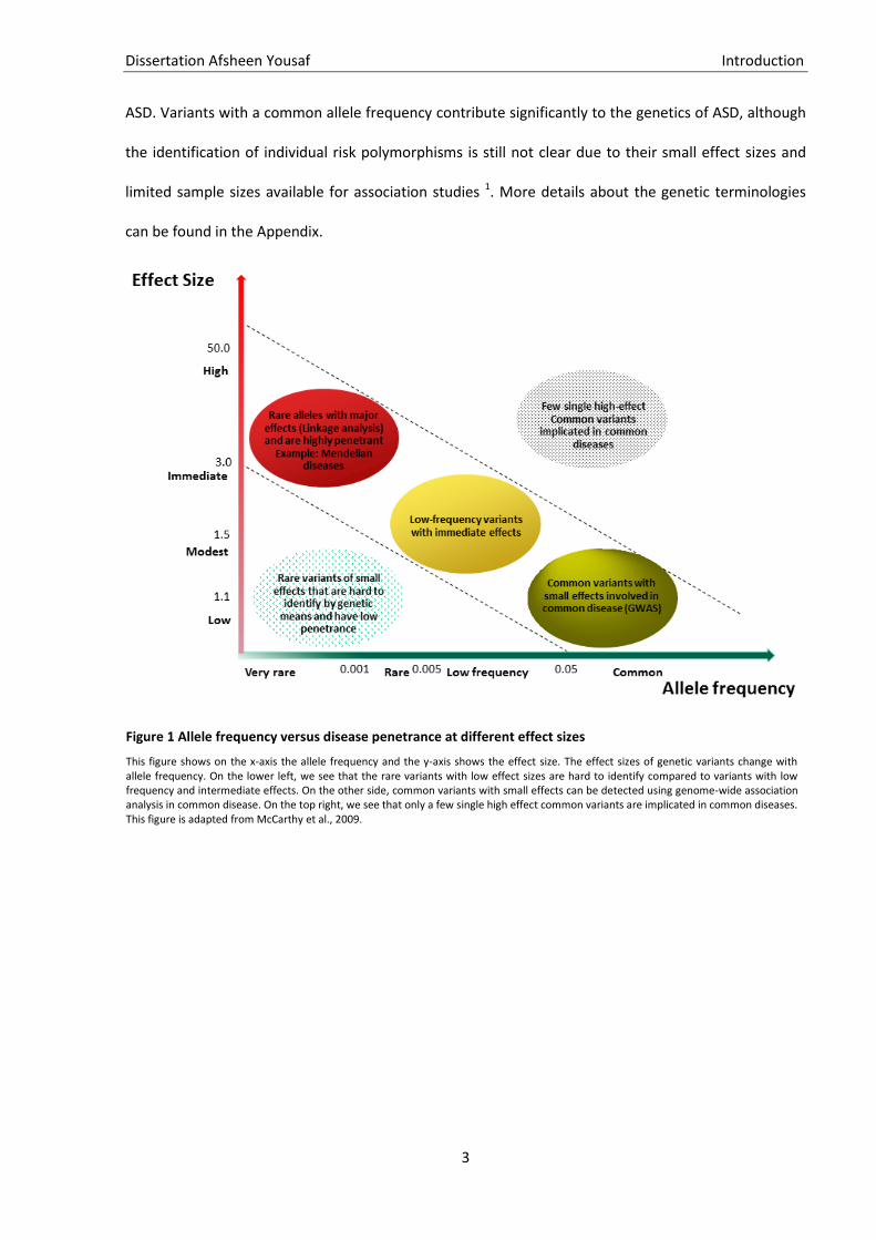
Dissertation Afsheen Yousaf Introduction
3
ASD. Variants with a common allele frequency contribute significantly to the genetics of ASD, although
the identification of individual risk polymorphisms is still not clear due to their small effect sizes and
limited sample sizes available for association studies 1. More details about the genetic terminologies
can be found in the Appendix.
Figure 1 Allele frequency versus disease penetrance at different effect sizes
This figure shows on the x-axis the allele frequency and the y-axis shows the effect size. The effect sizes of genetic variants change with allele frequency. On the lower left, we see that the rare variants with low effect sizes are hard to identify compared to variants with low frequency and intermediate effects. On the other side, common variants with small effects can be detected using genome-wide association analysis in common disease. On the top right, we see that only a few single high effect common variants are implicated in common diseases. This figure is adapted from McCarthy et al., 2009.
Dissertation Afsheen Yousaf Introduction
4
Types of data in genetic studies 1.3.
1.3.1. Phenotype data
Neuropsychiatric disorders generally come with a discrete diagnosis. For example, although the ASD
phenotype is discussed to be at the far right end of a normally distributed behavioral phenotype in the
general populations, the most frequent kind of available data is as categorical diagnosis. Interestingly,
the categorical diagnosis of ASD is usually based on quantitative phenotypic data, as generated during
the clinical assessments 83. These can include physical examinations, a series of interviews, cognitive
and personality tests. The diagnostic instruments are clinical interviews conducted by expert clinicians
from the (1) parent, primary caretaker or teacher, e.g. the ADI-R (Autism diagnostic interview-Revised)
13or (2) directly from the individual, e.g., the ADOS (Autism diagnostic observation schedule) 34.
The challenges faced for generating and retrieving phenotype data include standardized assessment
instruments that are harmonized across the sites, maintaining clinical records and dealing with missing
phenotype data due to lack of information gathered from the participants in the study data. However,
it is possible to fill the missing information using imputation techniques (see 2.4).
1.3.2. Genotype data: Types and Technologies
Genotype data comprises of genetic variants, which can be varying stretches of several megabases, i.e.
Copy Number Variants (CNVs) down to Single Nucleotide Polymorphisms (SNPs) or Single Nucleotide
Variants (SNVs). To obtain genotype data, there are two widely used technologies, i.e. array-based and
next-generation sequencing technology described as follows:
Array-based technologies
Millions of SNPs can be genotyped using oligonucleotide (short DNA molecules)-probes with the main
purpose to differentiate between alternative alleles at the SNP locus and determining the nature of the
allele based on the signal generated from genotyping. The two key players in this technology are
Affymetrix and Illumina. Both technologies are based on the biochemical principle that nucleotide
bases bind to their complementary bases based on Watson–Crick base pairs, i.e. A (Adenine) pairs with

Dissertation Afsheen Yousaf Introduction
5
T (Thymine) and C (Cytosine) pairs with G (Guanine). Moreover, both the technologies call for the
hybridization (annealing) of fragmented single-stranded DNA to arrays which contain millions of unique
nucleotide probe sequences designed specifically to a target DNA subsequence. However, Illumina has
a higher probe density that encompasses millions of markers.
Affymetrix arrays take a short DNA sequence targeting a single SNP allele. There are unique nucleotide
probes which are designed in a way that they serve as perfect complementary to one of the two or
more target alleles, e.g. A or B of a genetic variant (Major alleles conventionally referred to as allele A).
Besides that, there are also negative probes that are identical to a perfect matching probe except that
the allele-specific base is altered such as not to be complementary to any of the annotated alleles 35.
After the hybridization of target DNA to these unique nucleotide probe sequences, a signal is
generated, and its intensity is measured. The intensity is proportional to the amount of target DNA in
the sample and depending on the affinity between the target and probe. These intensity measures can
depict the SNP genotype, i.e. AA, AB or BB 35. Since intensity measures of all probes and individuals are
assessed on multiple arrays, the intensities are normalized to account for non-biological differences.
This aims at standardizing the intensity distributions across the arrays. The standardized approach is
quantile normalization. It ranks the data and makes each quantile the same across the sample by
calculating mean or median. In this manner, an average of the distributions is generated. So the
highest values in the samples are the mean highest values. This ensures that all arrays in the study
have precisely the same probe intensity distribution 35. This can be achieved by implementing
normalization algorithms in any programming language such as R, MATLAB, etc.
Illumina Bead-Arrays are based on the single base extension technology Infinium. Here, two allele-
specific probes are designed to bind adjacent to the SNP of interest. The last base of the probe
matches the alleles of interest. A single base extension is used to confer the allele specificity of the
probe. For example, if a probe is a perfect match to allele A, a nucleotide with a green fluorophore is
incorporated and a red fluorophore for the B allele. Illumina uses silica beads (a few microns in size)
and a longer probe sequence than Affymetrix. In addition, a genetic barcode is attached to the bead in
Dissertation Afsheen Yousaf Introduction
6
the form of another oligonucleotide with a fluorescent dye to be able to allocate the specific probes 36.
For each variant, beads with specific probes (one per bead) are synthesized and spread randomly on to
a glass slide with silica coating having small etched holes for the beads to reside 37. Thus, each SNP is
interrogated with a single bead type covered by one unique probe designed to target the sequence
spanning the SNP of interest. The signal intensities from each bead type are measured with a
scanner 38. A number of algorithms are available for processing the raw signal from these arrays into
genotype calls such as GenCall 39 and BeadStudio/GenomeStudio software; Illumina 40. Normalization
steps are performed at the level of sub-bead pools level 39 (SNPs that share similar properties and are
usually clustered together) using Illumina BeadStudio software, which provides the normalized
intensities as a pair of coordinates corresponding to the signals for the two alleles at each SNP 40.
NGS technologies
NGS (Next-generation sequencing) is a DNA sequencing technology that performs millions of
sequencing reactions of multiple small fragments of DNA to determine the sequence. Thus due to the
speed of sequencing and the amounts of data generated this technology is also termed “high-
throughput”. It has massively reduced the time and cost required to generate sequence data. The
sequencing methods vary depending on the retrieval of DNA/RNA samples such as healthy vs. affected,
different time points and experimental conditions, etc.
NGS provides large-scale DNA sequencing and is an efficient technique to identify novel SNPs 41. NGS is
used for sequencing a whole-genome or targeted regions of the genome, e.g. coding regions, exome-
sequencing, which are sheared into small fragments. Barcodes and adapters are attached to each of
the fragments for sequence identification, and each fragment is converted into a sequencing library. In
the next step, the individual sequences are amplified multiple times and are sequenced. These
sequences are then mapped and aligned onto annotated reference genomes, e.g. the human genome
19 reference (hg19). After aligning the fragments, SNP or genotype calling can be performed to identify
SNPs and genotype for each individual respectively 42.
Dissertation Afsheen Yousaf Introduction
7
Array technology uses pre-selected targets whereas sequencing provides better coverage of the entire
genome. Since the focus of this research is on common variants, which can also be covered by SNP
genotyping technologies and are less expensive than the sequencing technology, we performed SNP
genotyping only.
1.3.3. Transcriptome data
Transcriptome data is a representation of the complete set of RNA transcripts produced by the
genome under specific circumstances such as the effects of a drug at specific time intervals or in a
specific cell. For example, this data can contain information about the gene expression at certain time
points and/or tissues in an organism. The two widely used platforms for generation of transcriptome
data are microarrays and RNA-sequencing, both relying on the conversion of RNA into cDNA, i.e. the
complementary DNA sequence to the respective transcript.
Microarrays are cost-effective and measure the abundance of transcripts via hybridization of the cDNA
to an array of complementary probes, similar to the genotyping arrays, but targeting cDNA specific
sequences. RNA-Seq is an NGS method, short pieces of cDNA (adapters) are attached to these
fragments which contain the sequences to amplify the genomic fragment. These adapters also contain
short sequences that serve as identifiers to avoid the samples being mixed. The cDNA library is then
analysed by NGS, which produces short sequence segments corresponding to either one or both ends
of the fragment. These short segments are then reconstructed and aligned with the help of a reference
genome such as 1000 Genomes to map the genes. In the end, raw counts are produced, which are the
number of reads that overlap with a transcript. In both cases, the data is normalized and analysed with
the help of various bioinformatics tools available, e.g. the data analysis package limma in R 43 and also
as standalone software that can analyse gene expression data and identify specific patterns, e.g.
dCHIP 44 for microarrays, ArrayAnalysis 45 and AltAnalyze 46.
Dissertation Afsheen Yousaf Introduction
8
ASD 1.4.
1.4.1. ASD prevalence and diagnosis in research
ASD is a neurodevelopmental disorder marked by impairments in two domains, i.e. (A) social
interaction and communication, and (B) restricted or repetitive patterns of behavior and interests.
The estimated prevalence of ASD was 2.47% among the United States children and adolescents in the
years 2014-2016 47. The median of global prevalence estimates of ASD was 62/10,000. This estimated
prevalence is four times higher in boys than girls 48. Despite these high prevalence rates of ASD and
efforts to reveal its genetic basis over the past decade, a clear understanding of the ASD mechanism is
still unresolved.
Currently, there are two gold standards for the diagnosis of ASD, i.e. the ADOS 34 and the ADI-R 49. They
provide a diagnostic algorithm for the ICD-10 (International Statistical Classification of Diseases and
Related Health Problems- 10th Revision) 50 and DSM-IV-TR (Diagnostic and Statistical Manual of Mental
Disorders, 4th Edition-Text Revision) 51 definitions of ASD 52.
Both ADI-R and ADOS are well established and validated diagnostic tools for children and adolescents
with ASD. As mentioned before that the data gathered from these diagnostic tools can be interpreted
as quantitative or phenotype data. In this study, we used ADI-R data because it considers the actual
state of the patient as well as information on the retrospective behavior over the years and is thus less
prone to age effects. Furthermore, the ADI-R, in contrast to the ADOS, does not come with age or
developmental specific versions.
1.4.2. Genetics of ASD
Heritability
ASD is one of the most genetically heritable mental disorders but lacks information available on its
neurobiological causes and biomarkers. One of the biggest challenges in understanding the mechanism
of ASD is its heterogeneous clinical and genetic architecture. Moreover, the strong interplay of genetic
influences and environmental interactions makes it a topic of intriguing research. Twin studies have
Dissertation Afsheen Yousaf Introduction
9
also assisted in estimating the genetic and environmental contributions of ASD phenotypes. These
studies have shown that MZ (monozygotic) twins are more concordant (twins sharing the same genetic
and environmental condition) for ASD than DZ (dizygotic) twins (twins sharing environmental
conditions but only 50% of their genetics) suggesting strong genetic effects underlying the liability to
ASD 54. A meta-analysis of twin studies estimated heritability rates between 64% - 91% 55. Another
recent study estimated the heritability of ASD in population data from five countries and found an
estimate of ~80%, further supporting the finding that variation in ASD occurrence in the general
population is mostly attributed by inherited genetic influences 56. Besides that, the risk of ASD has been
shown to be increased by genetic variants 57, structural variations 28, and mutations 58.
Genetic architecture of ASD
The underlying causes of ASD remain largely unknown however twin studies have shown a high genetic
contribution to ASD 59. Based on the Human Reference Genome Project an individual on an average
carries 3 million genetic variants that differ from the reference human genome 60. These variants could
be SNPs/SNVs, CNVs, and short insertions or deletions also termed as indels. All these variants
contribute significantly to ASD liability. Moreover, the type of variants (common or rare), as well as the
origin of variants (inherited or de novo), contribute to the ASD genetic risk. Though, common variants
are known to have small effect sizes but increase genetic liability for ASD. Previously, a twin study in a
Swedish sample has identified that the genetic variation accounts for ~60% of the liability for ASD with
common variants accounting for ~49% of the liability 62. On the contrary, de novo mutations, CNVs and
gene disrupting point mutations (a single nucleotide base change that can disrupt gene function)
collectively contribute ~5% of the ASD liability 73 and less heritability.
Dissertation Afsheen Yousaf Introduction
10
Genetic studies designs 1.5.
1.5.1. Twin studies in ASD
These studies evaluate the involvement of genetic and environmental factors on complex diseases
based on the findings that MZ twins share 100% of genetic makeup and DZ twins share ~50% of their
genetic makeup, while both share the same environment. High co-twin correlations among MZs and
low co-twin correlations among DZs would suggest a high genetic heritability. Similarly, a high co-twin
correlation among both groups would indicate a strong environmental effect on the phenotype. Twin
studies are generally used to assess the heritability of a phenotype and thus to inform the decision to
investigate a trait at the genetic level.
The first twin study of ASD was performed by Folstein et al.,1977 in a cohort of 11 MZ twins and 10 DZ
twins. The study identified that MZ twins were more concordant for ASD, i.e. 36% compared to 0% for
DZ 77. However, when a ‘‘broader autism phenotype’’ (individuals with personality and cognitive traits)
was used, the concordance rate increased to 92% for MZ twins and to 10% for DZ twins 54,78,79. In the
later period, twin studies with comparatively larger groups than the previous studies showed high
concordances for ASD in MZ twins (77–95%) compared with DZ twins (31%) 80. Moreover, these studies
have shown that the recurrence of having a child with ASD can increase depending on the proportion
of the genome, which is shared between the individual and an affected sibling or parent.
Sandin et al. 81 showed that individual risk of ASD and autistic disorder is increased with genetic
relatedness to an individual with ASD. They estimated the relative recurrent risk (RR) for ASD as
compared to the general population was RR= 153.0 (95% CI (Confidence Interval), 56.7-412.8) for MZ
twins, RR= 8.2 (95% CI, 3.7-18.1) for DZ twins, RR= 10.3 (95% CI, 9.4-11.3) for full siblings, RR= 3.3 (95%
CI, 2.6-4.2) for maternal half-siblings, RR= 2.9 (95% CI, 2.2-3.7) for paternal half-siblings and 2.0 (95%
CI, 1.8-2.2) for cousins. In this study, the heritability of ASD and autistic disorders is estimated to be
~50% for the additive genetic component and similarly, the non-shared environmental influence was
also 50%. In a recent meta-analysis by Tick et al. 55, the correlations for MZ twins were 0.98 and for DZ
Dissertation Afsheen Yousaf Introduction
11
0.53 at a prevalence rate of 5%. Another study by Sandin et al. 2017 8 included 37,570 twin pairs,
2,642,064 full sibling pairs, and 432,281 maternal and 445,531 paternal half-sibling pairs. Among these,
14,516 children were diagnosed with ASD. The ASD heritability was estimated to be 83%, non–shared
environmental influence was 17%. In short, these studies have provided high heritability estimates of
ASD. One limitation, however, is that these estimates are often overestimated due to the overlapping
genetic makeup between MZ twins and the 50% similarity in DZ twins. Finally, these studies do not
provide information on the chromosomal regions, genes or variants involved. For this purpose, linkage
studies and whole-genome analyses are performed.
1.5.2. Linkage studies in ASD
The purpose of linkage studies is to evaluate the probability that an allele or set of alleles are inherited
together with a disease or trait in a family or group of families and thus to map the phenotype onto a
genomic location, rather than identifying causal variants. The analysis is conducted in large pedigrees
and tests for genome-wide genetic markers. The results are expressed as LOD (logarithm of odds)
scores which compare the likelihood of two loci are being linked to the phenotype, i.e. being co-
inherited, with the likelihood of observing them by chance in a disease 82. High LOD scores thus
correspond to regions with strong linkage to the disorder, i.e. the unknown disorder locus is close to
the linked variants and can contain several candidate genes that are then investigated further.
A large number of linkage studies have identified ASD risk loci on multiple chromosomes, i.e. 2q21-33,
3q25-27, 3p25, 4q32, 6q14-21, 7q22, 7q31-36, 11p12-13 and 17q11-21 64. A study by Liu et al. 83
showed that dimensional subphenotypes of ASD can also help in reducing the genetic heterogeneity
and can lead to better identification of susceptibility loci. In ASD families with IQ (Intelligence Quotient)
≥ 70, they identified linkage to chromosome 15q13.3-q14, a region already known in SZ. Moreover,
they also found linkage of chromosome 11p15.4-p15.3 with “delayed onset of first phrases”. Later, the
same group identified loci in a large study cohort associated with specific phenotypes in ASD. For
example, the region 19q13.3 was genome-wide significantly associated with repetitive sensory-motor
behavior (RB) whereas 11q23 was associated with joint attention (JA) 84. Later, Weiss et al. 85
Dissertation Afsheen Yousaf Introduction
12
performed a genome-wide linkage study and identified suggestive and significant linkage on
chromosomes 6q27 and 20p13, respectively. Further analysis showed SNP on chromosome 5p15
between SEMA5A (Semaphorin 5A) and TAS2R1 (Taste 2 Receptor Member 1) was significantly
associated with ASD (P= 2x10⁻⁷). They also identified that the expression of SEMA5A is reduced in the
brains of autistic individuals.
Linkage analyses are suitable to detect loci and subsequently genes with potentially rare variants of
high penetrance. However, they are not able to detect common variants that have small individual
effects on risk 86. GWAS is a powerful method to detect common variants with small effect as seen in
Figure 1.
1.5.3. Genome-wide association studies in ASD
Though association studies are designed for any type of genetic variants, SNPs are mostly used because
of their spread across the genome. GWAS methods can analyse variations in a case-control or trio-
based (parents and offspring) setting. GWAS is efficient in detecting common alleles that contribute to
common multifactorial diseases 87, however not only limited to common variants. GWAS is based on
genotyping data usually generated using Chip- Array technology (see 1.3.2). Since the number of SNPs
is limited to these arrays genotype imputation is further used to infer the missing genotypes based on
linkage and thus increasing the number of SNPs to be analysed (see 1.7.2).
In trio-based studies, an affected individual is recruited along with the parents to compare the alleles
transmitted from the parents to the case versus the non-transmitted. This is performed by using the
TDT (transmission-disequilibrium test), which looks for the linkage between a marker allele and a
disease locus. One limitation of TDT is the difficulty to recruit parents-case data.
Association studies based on case-control design have controls that are either unrelated or are the
family members of the individual. In this study design, the occurrence of a given allele in cases versus
the controls is observed to see the association between the phenotype and the disease. In contrast to
a Chi2 (chi-square)-based association test as used in case-control studies, the TDT approach is
Dissertation Afsheen Yousaf Introduction
13
independent of potential stratification effects, i.e. findings that might relate to the differences in
ethnicities between cases and controls rather than the group status.
A caveat in GWAS studies is that millions of SNPs are tested. Testing for multiple corrections is
therefore mandatory to minimize the chances of false positives. The two widely used methods are FDR
(False discovery rate) 88 and Bonferroni 89 correction which calculates the expected rate of type I errors
when performing multiple comparisons which then provide a corrected p-value (see Appendix).
Generally, the larger the sample size, the more likely a study will find a significant relationship if it
exists. As the sample size increases, the impact of the random error is reduced and the overall
variability is decreased. This allows the measures to become more precise for the complete dataset.
However, with large study cohorts, more bias can be introduced in the analysis, such as various
confounding factors including population stratification (see 2.6.8), inadequate quality control and
genotyping errors. As well as performing GWAS on small underpowered samples can result in false-
positive findings. Examples for successfully identified associations have been reported for several
complex disorders such as ASD 90,91, Alzheimer 92, Parkinson’s 93, stroke 94, and SZ 95.
There has been a drastic increase in ASD-GWAS since the first successful GWAS in ASD by Wang et al.
2009 96 who identified six significant SNPs mapping to CDH10 (Cadherin 10) and CDH9 (Cadherin 9)
genes which encode neuronal cell-adhesion molecules. Another study by Anney et al. 97 found a
genome-wide significant SNP rs4141463 located within the gene MACROD2 (Mono-ADP
Ribosylhydrolase 2). Later, a study by Connolly et al. 98 selected individual items from the ADI-R, ADOS,
and the Social Responsiveness Scale (SRS) in the Autism Genetic Resource Exchange (AGRE) cohort to
perform GWAS. They reported eight genome-wide significant (P< 5×10⁻⁸) hits, i.e. rs10239799 (KCND2:
Potassium Voltage-Gated Channel Subfamily D Member 2) , rs2056412 (C8ORFK32: Family With
Sequence Similarity 135 Member B), rs2779251 (NOS2A: Nitric Oxide Synthase 2), rs1429793 (NELL1:
Neural EGFL Like 1), rs11899372 (BIN1: Bridging Integrator 1), rs4925506 (MPN2: Serine Protease 38),
rs17134117 (SDK1: Sidekick Cell Adhesion Molecule 1) and rs3797817 (FER: FER Tyrosine Kinase)
associated with “serious facial expressions”, “concentrating on parts of object rather than whole
Dissertation Afsheen Yousaf Introduction
14
picture”, “loss of motor skills”, “faints or blackouts”, “association of loss of skills with physical illness”,
“too tense in social settings” and “loss of motor skills”, respectively.
A study by Smoller et al. 99 analysed five psychiatric disorders namely ASD, ADHD, BD, Major depressive
disorder and SZ. SNPs at four loci mapping to regions on chromosomes 3p21 and 10q24 passed the
genome-wide significance threshold. A more recent GWAS focused on the seven items of the restricted
and repetitive behavioral score of the ADI-R in 3,104 ASD-affected individuals. It identified a genome-
wide significant association of the SNP rs2898883 (P< 6.8×10⁻⁹) with the degree of the repetitive use of
objects or interest in parts of objects100. This SNP is located within the sixth intron of PHB (Prohibitin).
On further investigation, they identified candidate target genes of the associated SNPs at that locus
and found three more genes: SLC35B1 (Solute Carrier Family 35 Member B1), CALCOCO2 (Calcium
Binding And Coiled-Coil Domain 2) and DLX3 (Distal-Less Homeobox 3).
In short, to date several studies have investigated the association of SNPs with ASD via GWAS but with
limited replication success. The reason is the limited sample size and small effects of disease variants,
and as a result, these associations are not replicated in other studies. With the advent of large-scale
international collaborations to combine genotyping data from different sites, the statistical power has
been improved. A recent genome-wide association meta-analysis of 18,381 ASD cases and 27,969
controls identified five genome-wide significant loci with the variants rs910805, rs10099100,
rs201910565, rs71190156 and rs111931861. It is the first study to robustly associate common variants
with ASD and further highlighted biological insights relating to neuronal function and corticogenesis 57.
1.5.4. CNVs studies in ASD
Beside SNPs, CNVs are another class of genetic variants that are being analysed. Overall 4.8-9.5% of the
human genome is affected by CNVs 101. Since CNVs include deletion, duplication or insertion of DNA
fragments their effect on gene expression could also be large. Therefore, they might also be related to
phenotypic variations in a genetic disorder. One problem with these studies is the accurate
determination of CNVs and their boundaries since they can vary among individuals 102. CNV studies,
similar to SNP studies rely on Array data comparing the intensity of signals across the genomic markers
Dissertation Afsheen Yousaf Introduction
15
to identify deletions or duplications. CNV studies are mostly done in trios to identify rare de-novo CNVs
in the affected individual that have not been transmitted by the parents. The term de-novo refers to
the new mutation, i.e. germline origin of the variant in the affected study participant. CNV studies have
found regions in genes associated with ASD103, type-2 diabetes 104, and SZ 105.
In addition to SNPs, CNVs are an important susceptibility factor for ASD. Studies have shown that the
proportion of de novo CNVs is three to five times higher in ASD families when compared to controls.
Altogether, they explain only 1% genetic heritability of ASD 28,68. De novo CNVs were found in ~ 27% of
individuals with syndromic ASD (associated with chromosomal abnormalities or mutations in a single
gene) 69. Individuals with two or more de novo CNVs typically have a more severe phenotype. Previous
studies have shown that in ~ 7-8% of individuals with ASD chromosomal anomalies were found 70.
Among the most common CNVs in ASD, there are the maternally derived duplications of chromosome
15q11-q13, as well as deletions of 16p11.2 and 22q13. Studies have also found a considerable
enrichment within CNVs in ASD for neuronal synaptic complex genes such as SHANK2 (SH3 And
Multiple Ankyrin Repeat Domains 2), SHANK3 (SH3 And Multiple Ankyrin Repeat Domains 3), NRXN1
(Neurexin 1), and NLGN4 (Neuroligin 4) 71,72.
CNV studies have provided important regions and genes associated with the ASD phenotype 3,68,72,106.
Previously identified genetic variants included CNVs associated with 7q11.23 107, 15q11–13 106, 16p11.2
68, and 22q11.2 28 loci, as well as genes NRXN1 108, CNTN4 (Contactin 4) 109, SHANK3 110, and NLGNs
genes 72. Among the pioneer studies for CNV analysis, a study by Szatmari et al., 2007 111 identified 254
highly significant CNVs. Out of these, four CNVs were highlighted and among them, a 300 kb sized CNV
deletion on chromosome 2p16 was identified in two families. This region contains coding exons of the
NRXN1 gene, which interacts with neuroligins in synaptogenesis. Hence, disruption of this region can
affect the function of NRXN1, which might affect ASD or its phenotypes.
Later, a study by Sebat et al., 2007 71 identified 17 de novo (occurs in children but not in their parents)
CNVs in 16 individuals. They identified a 4.3 Mb (Megabase) sized de novo deletion at 22q13.31-
q13.33, which includes the SHANK3 gene. This region has also been previously associated with ASD 112.
Dissertation Afsheen Yousaf Introduction
16
Another recurrently reported CNV region associated with ASD is located on the chromosomal region
16p11.2. Studies have reported microdeletions and microduplications of 16p11.2 which has been
validated further to be associated with ASD 28,113.
A whole-genome CNV analysis by Glessner et al.72 identified CNVs in the loci 15q11–q13, 22q11.21,
containing the ASD susceptibility genes NRXN1 and CNTN4. Other new susceptibility genes identified in
this study were NLGN1 (Neuroligin 1) and ASTN2 (Astrotactin 2).
Furthermore, Pinto et al.106 analysed the genome-wide features of rare CNVs in ASD. Based on 996
cases and 1,287 controls, they identified 5,478 rare CNVs. By examining parent-child transmission, the
authors found 226 de novo and inherited CNVs that were not present in controls. As a whole, ASD
cases were found to carry a higher number of de novo CNVs than controls (1.69 fold, P= 3.4x10⁻⁴).
A number of novel genes such as SHANK2 (SH3 And Multiple Ankyrin Repeat Domains 2), SYNGAP1
(Synaptic Ras GTPase Activating Protein 1), DLGAP2 (DLG Associated Protein 2) and the DDX53 (DEAD-
Box Helicase 53) – PTCHD1 (Patched Domain Containing 1) were found to be associated with ASD in
this study.
In another study in Han Chinese population, pathogenic CNVs responsible for ASD were
investigated 114. Genome-wide study of CNVs in 335 ASD cases and 1,093 healthy controls was
performed. They identified six CNVs at 6q26 that were extended on different exons of PARK2 (Parkin
RBR E3 Ubiquitin Protein Ligase) gene. PARK2 was one of the important genes with several case-
specific regions overlapped on it.
A recent study investigated 1,108 ASD and 2,458 SZ cases in a Japanese population. 29 clinically
significant loci were common in both disorders. Disease-relevant genes were identified in eight known
ASD and SZ associated loci, i.e. 3q29, 7q11.23, 15q11.2, 15q11.2-q13.1, 15q13.3, 16p11.2, 17q12, and
22q11.2 103.
1.5.5. NGS studies in ASD
There are a number of NGS methods available, however, in genomics, the most commonly used
methods are whole-genome sequencing (WGS), whole-exome, and de novo sequencing. WGS attempts
Dissertation Afsheen Yousaf Introduction
17
to sequence the whole genome, however, due to sequencing technically difficult regions of the
genome, it can capture only 95% of the genome. WES only considers the protein-coding sequences (i.e.
exome) for sequencing and offers less coverage than WGS. As WES only focuses on ~1.5% of the
genome that constitutes the exomes, the cost to sequence it is ultimately reduced compared to WGS.
De novo sequencing refers to the sequencing of a primary genetic sequence of a particular organism
for which there is no reference sequence available. NGS has been widely used in the identification of
variants associated with ASD 115, SZ 116 and depression 117.
Nowadays, NGS studies in ASD are extensively performed and have identified disruptive variants in the
protein-coding regions of the genome. One of the earliest NGS studies in ASD is from Sanders et al.,
2012 118. They performed WES of 928 individuals, which included 200 phenotypically discordant sibling
pairs with de novo mutations in brain-expressed genes associated with ASD. They identified a total of
279 de novo coding mutations and one gene named SCN2A (sodium channel, voltage-gated, type II, α
subunit) with de novo mutations in two affected individuals. Later, a study by Rubeis et al., 2014119
performed exome sequencing in 3,871 autism cases and 9,937 ancestry-matched or parental controls
individuals. They identified 22 autosomal genes at an FDR < 0.05, along with 107 autosomal genes.
Moreover, they identified that these genes are enriched for developmental pathways of chromatin
remodeling, synaptic function, etc.
Another WES study from 787 ASD families reported that ASD is associated with de novo indels
(insertion/deletion of a nucleotide base). The study also identified de novo indels in the genes of
KMT2E (lysine methyltransferase 2E), and RIMS1 (regulating synaptic membrane exocytosis 1) involved
in synaptic function and chromatin modification 120.
1.5.6. eQTL studies in ASD
An eQTL (Expression quantitative trait loci) represents a genomic locus or variant, e.g. a SNP that
influences the expression level of a gene. eQTLs can act in cis if the respective SNP is present near the
gene whose expression is influenced or they can act in trans, i.e. the SNP is not in close proximity to
the gene 121. Genome-wide eQTL mapping thus identifies the association between gene expression
Dissertation Afsheen Yousaf Introduction
18
levels and DNA variants (i.e. SNPs or CNVs) by performing a direct association test between markers of
genetic variation with gene expression levels across individuals. The analysis requires genetic markers
that can be genotyped in a population as well as data on the gene expression in the tissue of interest.
A direct association test is performed between markers of genetic variation with gene expression
levels. These analyses can help in identifying the underlying genetic mechanisms of diseases. For
example, when SNPs are associated with the expression of a gene in eQTL mapping and with a disease
in GWAS. This implicates that the expression of the gene mediates the effect of SNP on the disease 122.
eQTLs have been widely associated with ASD 123, BD 124, and SZ 125.
The relevance of eQTLs in neuropsychiatric disorders has been shown by a study which identified 21 of
the cis-eQTL variants of genes expressed in the fetal brain, that are located within a region of
chromosome 17q21.31 and are enriched among risk variants for ASD, ADHD, SZ and BD disorder 124.
Another study identified global enrichment of brain expression quantitative trait loci among top SNPs
from an ASD-GWAS including individual genes SLC25A12 (Solute Carrier Family 25 Member 12), PANX1
(Pannexin 1) and PANX2 (Pannexin 2) 126. Furthermore, a meta-analysis of 424 brain samples across five
different studies was performed to identify regulatory variants that influence gene expression in the
human cortex. They found that 28% of ~1000 autosomal genes encode proteins required for
mitochondrial structure or function were eQTLs (enrichment P= 1.3x10⁻⁹). Thus, the information
generated by eQTLs can provide important insight to understand the underlying biology of associations
with psychiatric disorders. Moreover, integrative strategies are also used combining results from GWAS
and eQTL to gather information on susceptible SNPs in GWAS such as in Crohn’s disease, SZ and
psoriasis 127–129.
ASD data 1.6.
1.6.1. Quantitative data
This type of data is gathered from clinical interviews such as ADI-R 49, or ADOS 34. which are the two
gold standards in ASD diagnosis (see 1.3). ADI-R is an investigator-based interview for parents or
Dissertation Afsheen Yousaf Introduction
19
caregivers of individuals with ASD. It comprises 93 questions, which are categorized based on (i) the
child’s early development; (ii) acquisition and loss of language; (iii) language and communication
functioning; (iv) social development and play; (v) interests and behaviors and (vi) general behaviors.
ADI-R focuses on behaviors that are less frequent in non-affected individuals, and therefore it is more
useful as an ASD-specific measurement. Studies have shown that ADI-R is influenced by the IQ,
language of the child, and age, as ADI-R is not recommended for children with non-verbal mental ages
of 18 months or below as well as children who have not started to walk 130,131. In addition, some
questions are only for verbal individuals. In ADI-R two separate scores are generated from social
communication (verbal and non-verbal communication) and the other for repetitive behaviors. The
answers are coded numerically between 0 and 9. 0 denotes that the behavior type specified in the
coding does not exist. 1 shows that the behavior type specified is present but not in severe form
whereas 9 denotes unknown or not asked question. A total algorithm score is then calculated for each
of the areas. An individual is diagnosed with ASD if the scores in every area exceed the cutoff threshold
for ASD.
1.6.2. Genotype data in ASD
SNPs and CNVs, both have an important role in the etiology of neuropsychiatric disorders, however
here, we only focus on SNP genotype data. The SNP genotype data is generally coded as A, C, G, T or 1,
2, 3, 4 but also as 1 or 2 for the major and minor alleles. The widely used genotype data formats are as
follows:
Merlin: This format contains a pedigree and a data file. The pedigree file includes the phenotype and
genotype relationships per individual per row. The first four columns contain identifiers for family,
individual, father and mother followed by gender information, where 1 is coded for male and 2 for
female. Next, the phenotype information is provided in the form of a qualitative or quantitative trait.
After this, genotype information for each individual is provided. The data file contains marker
information (M), affection status (A), quantitative trait (T) and covariate (C).
Dissertation Afsheen Yousaf Introduction
20
PLINK: This format consists either of files for pedigree (fam), SNP genotypes (bed) and SNP information
(bim), or flat format consisting of pedigree (ped) and SNP information file (map) (see Appendix).
Vcf (variant calling file): This format contains meta-information lines at the beginning of the file, a
header line consisting of chromosome number, SNP position, SNP id, alleles information, a quality
score, filter status (if the SNP is called at this position), and additional information followed by
genotype encoding.
Data analysis 1.7.
1.7.1. Quality Control
For quality assurance of genotype data, QC is a mandatory step before conducting any kind of analysis.
Quality thresholds are crucial and strongly dependent on the study design. Such as for performing
GWAS, a deep pre-processing and QC steps are required. Biases in study design and errors in genotype
calling can introduce a proficient amount of errors and information loss, which can increase the
number of false-positive and false-negative associations. To date, there are various QC pipelines and
protocols available, specifically used in psychiatric studies such as provided by the Ricopili 13 and the
ASC (Autism Sequencing Consortium) framework 119, as well as publicly available protocols 133.
However, there are only a few tools available to perform the QC followed by downstream analysis for
researchers with limited knowledge on handling complicated bioinformatics tools.
PLINK is one of the most widely used genetics tool which provides individual commands and options
for performing quality checks. The available automated tools to perform QC of genotype data include
SNPQC; an R-based pipeline for quality control of Illumina SNP genotyping array data 9. The pipeline
uses the direct output from Genome studio software that allows visualization and analysis of data
generated from Illumina 134. Since SNPQC is designed for Illumina arrays, it is dependent on files that
are directly provided by Genome studio and therefore might not be straightforward for the new users
Dissertation Afsheen Yousaf Introduction
21
with a limited programming background. Another available tool for QC is QCTOOL 135 but it is not
updated anymore and currently is legacy software.
1.7.2. Genotype imputation
Some individuals might have missing genotype data at loci, which are actually genotyped for another
fraction of individuals. The other scenario could be that the loci are not covered by the analytical
platform used. This missing data in association studies can be a limiting factor in terms of sample
inclusion and genotyping resolution. For example, these studies exclude individuals with missing
genotypes considering a complete case analysis 136. This not only reduces the sample size but can also
cause potential bias and loss in efficiency of further downstream analysis 137. Imputation of genotype
values at loci which are untyped in samples can thus help in improving the mapping of the disease-
causing variants, e.g. identify variants, which are not genotyped but are actually associated with a
disease phenotype. Imputing these untyped variants can thus finally highlight fine association signals
by imputing the un-typed causal variants based on SNPs in LD (Linkage Disequilibrium), i.e. the SNP
alleles or DNA sequences that are physically close together in the genome tend to be inherited
together and are in high LD rather than the SNPs far apart.
The quality of imputed data largely depends on the reference data selected for imputation, as the
unobserved genotypes in the study data set are predicted based on the haplotype (a particular set of
alleles that tend to be transmitted together) patterns in the reference panel. The two widely used
reference panels are HapMap and 1000 Genomes: The HapMap reference dataset was one of the
most used reference panels for imputation analysis in the beginning era of Genome-wide association
analysis. Phase 2 of the HapMap project contained 270 unrelated individuals from Africa, Asia, and
Europe. However, in phase 3 of the HapMap project, the number increased to 1,301 unrelated
individuals and also covered individuals from 11 different populations. The dataset included 3.5 million
commonly occurring genetic variants. This dataset had a deep coverage as it contained samples from a
variety of different populations. The 1000 Genomes dataset phase 1 was released in 2012 whereas
phase 3 was released in 2015. This is the largest reference dataset available for imputation with 2,504
Dissertation Afsheen Yousaf Introduction
22
individuals and 84.4 million variants. It provides wide coverage as it contains many more SNPs than the
HapMap data.
Imputation of genotype data relies on efficient and correct estimation of haplotypes which is improved
by the correct identification of an individual’s alleles inherited on one strand from one parent (phased
strands). The computationally most intensive step during imputation is pre-phasing; which estimates
the strand-based haplotypes (i.e. allele combinations inherited together on one strand) based on the
called GWAS genotypes. Pre-phasing before imputation speeds up the imputation performance 138, and
the pre-phased data can be used in the future on the availability of a new reference dataset. Thus,
having the pre-phased data saves time for imputation and before imputation, since, for each set, the
haplotype is estimated based on all the phased alleles. Haplotype estimation can also be performed in
unrelated individuals by modeling the haplotype frequencies. Since several haplotype combinations
are possible for an individual’s genotypes, one can estimate the probability of any given haplotype
configuration and choose the most likely configuration or output a set of configurations sampled from
the posterior distribution (see 2.7).
SHAPEIT is a widely used tool, which performs phasing. The other widely used tool to infer haplotypes
is Phase v2.1 139. SHAPEIT differs from it as it uses binary trees to represent the haplotypes for
everyone, which overcomes the haplotype inference limitations by speeding up the computations for
calculating posterior probabilities of the haplotypes compared to Phase v2.1. In addition, using the
binary trees, it looks for the most plausible haplotypes for haplotypes estimation. SHAPEIT has also
outperformed the previously used tools like Fastphase 140 and Gebril 141 in terms of speed and
accuracy.
To date, there are several genotype imputation pipelines available such as the “genipe” 142, “Molgenis-
impute” 11 and “Gimpute” 143 pipelines. Genipe uses PLINK 144, SHAPEIT 145 and IMPUTE2 138 software to
perform complete imputation. Molgenis-impute is a command-line tool that can be run on local
servers as well as high computational clusters and is also based on the SHAPEIT 145 and IMPUTE2 138
tools. Gimpute is an extension to the genipe 142 but with extensive pre and post imputation steps. All
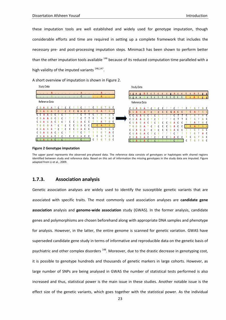
Dissertation Afsheen Yousaf Introduction
23
these imputation tools are well established and widely used for genotype imputation, though
considerable efforts and time are required in setting up a complete framework that includes the
necessary pre- and post-processing imputation steps. Minimac3 has been shown to perform better
than the other imputation tools available 146 because of its reduced computation time paralleled with a
high validity of the imputed variants 146,147.
A short overview of imputation is shown in Figure 2.
Figure 2 Genotype imputation
The upper panel represents the observed pre-phased data. The reference data consists of genotypes or haplotypes with shared regions identified between study and reference data. Based on this set of information the missing genotypes in the study data are imputed. Figure adapted from Li et al., 2009.
1.7.3. Association analysis
Genetic association analyses are widely used to identify the susceptible genetic variants that are
associated with specific traits. The most commonly used association analyses are candidate gene
association analysis and genome-wide association study (GWAS). In the former analysis, candidate
genes and polymorphisms are chosen beforehand along with appropriate DNA samples and phenotype
for analysis. However, in the latter, the entire genome is scanned for genetic variation. GWAS have
superseded candidate gene study in terms of informative and reproducible data on the genetic basis of
psychiatric and other complex disorders 148. Moreover, due to the drastic decrease in genotyping cost,
it is possible to genotype hundreds and thousands of genetic markers in large cohorts. However, as
large number of SNPs are being analysed in GWAS the number of statistical tests performed is also
increased and thus, statistical power is the main issue in these studies. Another notable issue is the
effect size of the genetic variants, which goes together with the statistical power. As the individual

Dissertation Afsheen Yousaf Introduction
24
variants carry only a small risk in disease traits, the effect size is smaller and more statistical power
(larger cohorts) is required to detect significant associations at the genome-wide level. To handle these
issues, gene-based analyses are applied after performing GWAS (see next section).
To perform GWAS analysis, there are existing pipelines like GWASpi 12, easyGWAS 149, and GWASTools
150. GWASpi is an application written in Java and can be used under Linux, Mac or Windows. It can be
used for pre-GWAS data quality control and conducting GWAS but has not been updated in recent
years. Another tool is easyGWAS, which is a web application that allows a user to upload the genotype
data and later retrieve the GWAS results. However, in most of the cases, genetic data is restricted to be
shared online. There are also several R packages and MATLAB functions available such as
“GWASTools”, “GWAS”, or one can also write own functions to perform GWAS depending on the
regression model and covariates.
1.7.4. Gene-based analysis for GWAS
In a GWAS, several millions of SNPs are tested and thus the significance threshold is set to a p-value of
5x10⁻⁸, based on the structure and best estimate of independent SNPs in the human genome. This
stringent threshold reduces the number of false-positive findings but also increases the number of
false negatives. However, the combined effect of weakly associated SNPs, which may or may not be
statistically significant on their own can predict the disease status or symptoms 151. Thus, to maximize
the use of GWAS, gene-based analysis provides an efficient way of combining the effects of individual
genetic variants to identify the collective effect at gene level 152. For polygenic traits, there is more than
one gene involved with thousands of genetic variants individually of small effects. This ultimately
requires large sample sizes to detect them. When analysing the collective effect of genetic variants, the
number of tests needed to be performed is considerably reduced thus allowing the effects of weaker
associations to be considered.
The success of GWAS analysis depends greatly on the available sample size. Here, gene-based analyses
have the potential to account for multiple independent functional variants within a gene that can thus
lead to an increase in power to identify the genes that are actually associated with the trait.
Dissertation Afsheen Yousaf Introduction
25
Among the most prominent tools used for gene-based analysis are MAGMA (Multi-marker Analysis of
GenoMic Annotation) 153 and VEGAS2 (Versatile Gene-based Association Study 2) 154. The functionality
of both tools is comparable. MAGMA can analyse both raw genotype data as well as summary SNP
p-values from a GWAS or meta-analysis. VEGAS2 is available as a web and command-line tool that
takes the GWAS summary file (output from GWAS) with SNP IDs and the association p-values. It first
assigns the SNPs to genes (17,787 autosomal genes) according to positions on the UCSC Genome
Browser hg19 assembly. It then searches for regulatory regions and SNPs which are in LD within
defined gene boundaries and positions around. The approach is permutation-based for testing the
enrichment for highly associated markers using the LD information from a reference panel so that all
the association signals from shared variants in LD can be detected.
MAGMA can use raw genotype data as well, where it first performs a principal component analysis
(PCA) for all the markers in each gene. MAGMA then performs a linear regression where it uses the
PCA eigenvectors as predictor variables and phenotype as the criterion variable. In this way, MAGMA
overcomes the problem of low statistical power which comes into existence when a gene contains
many markers and some of them are in strong LD. MAGMA also provides the option of performing
gene analysis on GWAS summary data (see 2.9). Thus, MAGMA is reported to be a distinctive tool
compared to other methods like INRICH 155, ALIGATOR 156, VEGAS 157 and MAGENTA 158 specifically
because of more statistical power, less affected by linkage disequilibrium and multi-marker
associations due to its multiple regression approach and being computationally less demanding 47. One
of the main differences between MAGMA and VEGAS2 is that MAGMA provides additional gene-set
analysis methods that can be categorized into self-contained and competitive analysis. The former
tests whether the gene set contains any association at all with a phenotype of interest and the latter
tests whether the phenotype association in the gene set is greater than in other genes.
1.7.5. Pathway enrichment analysis
Once the SNPs and their respective genes are associated with a disease phenotype, a further insight
into the functional effect of a SNP can serve as prime importance for understanding the underlying
Dissertation Afsheen Yousaf Introduction
26
mechanism of a disease. Such as at the biological system level by analysing their effect on signaling
pathways. To gain a mechanistic overview of any set of genes associated with a phenotype, pathway
analysis is an excellent approach. It can help to identify the underlying pathways and mechanisms. The
basic principle behind the analysis is to identify the biological pathways and gene ontology that are
enriched in a gene list more than what is expected by chance. For example, when looking for
annotations in the gene ontology, a standardized annotation platform of gene products, the frequency
of individual annotations in the significant gene list is compared to the complete list of all genes on the
array or in the human genome. In this way, a set of enriched biological processes annotated with the
respective genes is identified and allows to draw the conclusion that the trait of interest is underlying
alterations thereof. There are numerous pathway enrichment analysis tools, gene set enrichment
analysis (GSEA) and R packages available for performing these analyses such as Database for
Annotation, Visualization and Integrated Discovery (DAVID) 159, MetaCore 160, Ingenuity Pathway
Analysis (IPA) (QIAGEN Inc., https://www.qiagenbioinformatics.com/products/ingenuity-pathway-
analysis), Panther 161 and so on. MetaCore and IPA are high-end tools with very detailed information of
the pathways, its drug targets and interactive maps however these are not freely available. One of the
limitations of most of the tools is that it uses limited resources that are not timely updated such as
DAVID. In comparison, GO-Elite 162 is a web-based and a command-line tool that performs over-
representation analysis (ORA) and also accounts for the hierarchial semantic-structure of the GO
annotation terms. These GO annotations are always updated and automatically downloaded in GO-
Elite by default.
Aims of the study 1.8.
Genetics and neuropsychiatry are two individual fields, but to unveil the pathomechanisms underlying
complex neuropsychiatric disorders there is a strong urge to strengthen the methods and to develop
tools that can integrate data from different disciplines. These tools should be central for researchers in
genetics and neuropsychology to grasp and apply in research.
Dissertation Afsheen Yousaf Introduction
27
ASD is one of such complex developmental disorder that is diagnosed based on deficits in two
domains: (A) social interaction and communication and (B) restricted and repetitive behavior. In this
work, we incorporated two large ASD cohorts, i.e. AGP (Autism Genome Project) and a German cohort.
The overall aim of the study is to develop and evaluate an integrative bioinformatics Big-Data Pipeline
for the analysis of complex genetic traits in neuropsychiatry.
Therefore, we defined the following aims:
1. To elucidate the genetic architecture of quantitative ASD traits we first aimed at identifying and
validating independent behavioral subdomains based on available clinical assessments.
2. Generation of an integrative bioinformatics pipeline which can perform the following analysis:
i.Quality Control of the genotype data
ii.Genotype imputation
iii.Genome-wide association analysis
iv.Gene-based enrichment analysis
v.Brain enrichment analysis
3. To validate the implemented pipeline we applied MAGNET on the identified ASD subdomains in
two ASD cohorts to identify underlying genetic pathomechanisms associated with these individual
subdomains.
4. Further, our goal was to investigate if the phenotypically defined ASD subdomains are genetically
independent or are correlated with each other and if they share genetic etiology with ASD risk.

Dissertation Afsheen Yousaf Introduction
28
Dissertation Afsheen Yousaf Materials and methods
29
2. Materials and methods
ASD quantitative data 2.1.
In this study, we included a German cohort with individuals from n=705 families (n=625 parent-child
trios, n=53 parent-child duos, and n=27 singletons) recruited at the Departments of Child and
Adolescent Psychiatry at Goethe-University Frankfurt am Main, University Hospital Bern, Saarland
University Hospital, and University Hospital Freiburg. The other cohort is the AGP (Autism Genome
Project) cohort including n=2,730 trio families, and n=5 parent-child duos collected at 15 clinical sites
across the US, Canada, and Europe. Overlapping German samples were excluded from the AGP cohort.
The diagnosis was established by experienced clinicians based on thorough clinical assessment, the
Social Communication Questionnaire (SCQ) 163, ADI-R 49 and/or ADOS 164. Exclusion criteria and sample
quality checks were based on the AGP cohort 97. For the final analysis, only one affected individual per
family, i.e. the index patient, with complete ADI-R and genotype information available was included.
Written informed consent was obtained from all participants or caregivers, and the study was
approved by the local ethical committees (decisions 162/99 (Frankfurt); 147/10 (Aachen); 214/10
(Bern); 73/04 (Homburg), 237/09 (Frankfurt)). All ASD individuals were diagnosed according to ICD-10
165 by experienced child psychiatrists or clinical child psychologists. The diagnosis was confirmed by the
ADI-R 49,166 and/or ADOS 34. Individuals with SZ, BD, a neurodegenerative disorder, a known cytogenetic
finding, fragile-X Syndrome, Angelman syndrome, Prader-Willi syndrome, Rett syndrome or any other
genetically diagnosed disorder, IQ<35, history of a severe medical condition, birth weight <1,500 grams
or cerebral palsy were excluded. Sample quality checks and exclusion criteria are published
elsewhere 97.
Dissertation Afsheen Yousaf Materials and methods
30
SNP genotype data 2.2.
In this project, we focused on SNPs genotype data. The German cohort was genotyped using Illumina
HumanOmniExpress 12v1-H bead arrays at Life and Brain (Bonn, Germany). The AGP cohort was
genotyped on 550K Illumina, 510K Illumina, 1M Single and 1M Duo Illumina Chips 97. The methods
implemented for performing QC of the genotype data are detailed in 2.6.
SNP genotype data carries information of each SNP with an identification number, i.e. an “rs” number
or the chromosome number and genomic position, e.g. 7:24926377 where 7 is the chromosome
number and 24926377 is the genomic position. Besides this information about chromosome number,
physical position (Distance between two markers measured by the number of nucleotides between
them) and genetic position (Distance between chromosome positions) is also provided. Moreover, it
also includes a file consisting of sample information encompassing the pedigree and individual
information. The raw intensities from the array are then normalized and SNPs are called using specific
algorithms 167. The information can then be coded in PLINK format, i.e. as a ped and map or as bed, bim
and fam files. For a detailed description of the SNP genotype files that can be provided as input to our
developed pipeline please see Appendix.
I. Preliminary data analysis of phenotype data
Quality assurance of ADI-R data 2.3.
We focus on ADI-R data in our study which has a total of 93 items organized into specific categories
(see 1.4.1). Among these 93 ADI-R items, 42 are methodically combined in the form of a formal,
diagnostic algorithm for autism or a general diagnosis of ASD. We selected 28 “ever/most abnormal”
items from ADI-R questionnaire based on the study by Liu et al. 84, where “ever” denotes if a behavior
ever occurred and “most abnormal” represents whether the behavior was present at a specific,
defined period between 4 and 5 years of age. A list of these 28 items is provided in Table 3 in the
results section. These items are available for both verbal and non-verbal individuals. ADI-R diagnostic
Dissertation Afsheen Yousaf Materials and methods
31
algorithm scores of 3 were recoded as 2 to limit the impact of severity before performing phenotype
imputation. Moreover, it was made sure that all items use the same coding in both cohorts such as
item “Repetitive use of objects” used 7 as a score, which means that the individual shows a not age-
related interest in a toy, but this play cannot be designated into a high-grade stereotype, therefore it is
coded as 0 in both cohorts. Similarly, item 31: “Use of others body to communicate” codes 8 for little
or no spontaneous communication, which was then coded as 0 in both cohorts. Besides these
instances, all 8 and 9 scores were coded to NA (Not available). All individuals who had >10% missing
items in the 28 selected items were excluded from both cohorts. The item with the highest value
between the ever or most scores was selected for imputation. As the sample size is an important factor
affecting the statistical power and for reliable estimates, respective ADI-R items from AGP and German
cohorts were combined for phenotype imputation.
Phenotype imputation of missing ADI-R data 2.4.
In psychiatric research, it is a common problem that the clinical interviews used for diagnosing the
disorder, e.g. in ADI-R some questions are left unanswered. Multiple imputation (MI) is a statistical
technique for analysing incomplete data sets. MI fills the missing values multiple times and creates
multiple “complete” datasets. Multivariate imputation by chained equations (MICE) was implemented
in R using mice 168 package.
MICE is one of the most powerful techniques in current research to deal with such data 169. We
performed MI based on predictive mean matching (pmm) which is a semi-parametric imputation
approach. It aims at reducing the bias introduced in a dataset because of imputation and looks for real
values sampled from data170. MI using pmm is performed as follows:
i. Let us assume a variable Y which is to be imputed based on X predictors.
ii. Estimate a linear regression of Y on X producing 𝛽.
iii. A random draw from the posterior predictive distribution of 𝛽 is made to generate a set of 𝛽*.
Based on Bayesian inference, the information about unknown parameters is expressed as a

Dissertation Afsheen Yousaf Materials and methods
32
form of the posterior probability distribution to create random variability in the imputed
values 168.
iv. Using 𝛽*, the missing values are predicted for all cases with and without data missing on Y.
v. In each case where Y is missing, the closest predicted value is identified among the cases
where Y is observed.
vi. pmm then randomly draws one of the three close cases and imputes the missing value Yi with
the observed value of this close case.
vii. Depending on the m, i.e. number of multiple imputed datasets, to generate the algorithm, the
process is repeated m times in a chain. As a result, m complete datasets are generated.
We created 10 imputations, a number between 5-10 is suggested as computationally feasible as
suggested by Horton et al. 171, one dataset out of these m multiply imputed datasets was selected for
further analysis.
Identifying ADI-R subdomains 2.5.
An interesting approach for looking at the quantitative data is to identify meaningful groups or
subgroups to target the underlying genetic associations. Commonly used approaches to dissect the
heterogeneous architecture of ASD is to perform factor analysis 84,172 or principal component analysis
173,174. These analyses can firstly help in reducing the number of variables to more representative and
meaningful factors. Secondly, specifically looking at the individual subgroups helps in decreasing the
overall heterogeneity of the disorder and working on more homogenous groups.
PCA was preferred over the classical EFA (Exploratory factor analysis) approaches to preserve the
maximum amount of variation and independence in the resulting factors. This can play a role in
determining that the genetic factors might be independent of each other. EFA does not account for the
maximum variation and estimates interdependence between variables to find common factors, which
might not necessarily be independent of each other.
Dissertation Afsheen Yousaf Materials and methods
33
Following criteria were satisfied before performing PCA:
i. Sample size: A sample size of total n=50-400 is recommended to yield reliable estimates 175,176.
ii. Factorability: Checks that some correlations should exist among the variables so that coherent
factors can be identified. It is expected that the variables have a degree of co-linearity among
the variables but not an extreme degree or singularity among the variables. The following two
tests are performed for structure detection:
a. Bartlett’s test of sphericity: The null hypothesis is that the correlation matrix calculated for the
variables in the samples is an identity matrix. Whereas the alternative hypothesis is that they
are related and a structure could be detected. The purpose is to identify if there are redundant
variables in the samples, which can be summarized into a few numbers of components. The
test checks if the observed correlation matrix R= (rij)(pxp) (where p is the number of variables)
diverges significantly from the identity matrix. A significant result indicates that a principal
component analysis is appropriate for the data set.
b. Kaiser Maier Olkin (KMO) test: KMO also indicates the suitability of the data for structure
detection. The KMO measure of sampling adequacy is a statistical test that indicates the
proportion of variance in the items that might be caused by the underlying components. High
values close to 1 indicate that performing a PCA would be useful.
A partial correlation is calculated first which is the relation between two variables and removes
the effect of remaining variables. In the next step, KMO index compares the values of
correlations between variables and those of the partial correlations. If two variables share a
common factor with other variables, their partial correlation will be small, indicating the
unique variance they share.
∑∑
∑∑ ∑∑
where rij is the correlation matrix and aij is the partial covariance matrix

Dissertation Afsheen Yousaf Materials and methods
34
Based on the Kaiser’s criteria a KMO value between 0.9 -1 is considered best177.
2.5.1. PCA
PCA is a powerful tool to highlight similar patterns, similarities, and differences in the data. This
approach is very useful when dealing with multidimensional data. After the identification of patterns,
the data is compressed by reducing the total number of dimensions. We applied PCA to identify the
structure and dimensions of the quantitative trait data. The steps performed in PCA are as follows:
i. All initial variables are standardized so that each contributes equally to the analysis.
Mathematically this is done as follows:
ii. Calculation of the covariance matrix to identify the variation in variables from the mean with
respect to each other. Moreover, it reveals the relationship of the variables among each other.
Also if they are highly correlated in such a way that they contain redundant information.
A covariance matrix is then simply a symmetric matrix with nxn dimensions and has all possible
combinations of variables. For example, for a 3-dimensional data set with 3 variables x, y, and
z, the covariance matrix is a 3×3 matrix A of this form:
[
( ) ( ) ( ) ( ) ( ) ( ) ( ) ( ) ( )
]
Whereas cov(x,x)=var(x) in the main diagonal and cov(x , y) = cov(y , x) so the upper and lower
half of the diagonal is the same.
iii. Computation of the eigenvectors (principal components) and eigenvalues (explains how much
variance is present in the data) of the covariance matrix A. This can be expressed as:
where v is a vector, λ is the eigenvalue associated with eigenvector v of A. The eigenvalues of A
can be rewritten as ( ) where I is an identity matrix. Simplifying the matrix and
calculating the determinant will provide the eigenvalue of the matrix and the corresponding
eigenvector.
Dissertation Afsheen Yousaf Materials and methods
35
iv. Arranging the eigenvectors in descending order of eigenvalues will provide principal
components in order of significance. Eigenvectors with the lowest eigenvalues contain the
least information about the distribution of the data. The number of components is equal to the
number of dimensions of the data. But, PCA tries to put maximum information in the first
component.
v. Rotation
For a meaningful interpretation, it is necessary to spread the variability more evenly among the
components. Rotating the components will help in serving a simple structure. We chose
“varimax” rotation, which is an orthogonal rotation of the component axes to maximize the
variance of the squared loadings of a component (columns) on all the items (rows) in a
components matrix. The loadings from PCA are the weights and correlations between each
variable and the component. The higher the loads the more relevant it is in defining the
component. PCA was performed with varimax rotation on 28 ADI-R items using the R package
psych 178 as in previous studies 173,174.
vi. Component extraction
Components are extracted based on the following three criteria:
-Scree plot and Eigenvalue: A scree plot shows the eigenvalues of the principal components on
the y-axis and the number of factors on the x-axis. The point where the slope of the curve is
leveling off (“the elbow”) indicates the possible factor solution.
-Communalities: The proportion of variance accounted for each variable by the principal
components variables. Small values indicate variables that are not well represented in the
common factor space and vice versa.
-Total variance explained: Total amount of variability of the original variables explained by
each principal component.

Dissertation Afsheen Yousaf Materials and methods
36
vi. Interpretation of component loadings
The rotated factors should make a theoretical sense to the researcher. Each of the identified
components should have at least three variables with high loadings and each variable should
load highly on only one component.
The best solution for the number of components to be included was identified based on Kaiser’s
criterion i.e. to exclude all components with eigenvalues under 1.0 179, and scree plot 180. Components
were retained if (i) each component have at least three items loaded onto it 181,182, however, additional
variables improve stability 183; (ii) loadings of respective items >0.4, which is more stringent than
otherwise defined criteria (>0.35) 184; and (iii) they are interpretable. The respective items were
summed up to provide a combined score, which will be used for subsequent analysis.
Dissertation Afsheen Yousaf Materials and methods
37
II. The MAGNET tool: Implemented methods
Development of MAGNET was divided into five main parts, i.e. I) quality check (QC) of the genotype
data, II) imputation of genotype data, III) GWAS, IV) enrichment analysis, V) integration of
transcriptome data. This section details all the methods and algorithms implemented within MAGNET
and the respective criteria used within each part. The list of software used for the analysis is provided
in Table 1.
Tool Description PLINK v 1.9 (Purcell et al., 2007) Genetic data analysis
liftOver (Tyner et al., 2017) Converts between genome builds
SHAPEIT v2.727 (Delaneau et al., 2011) Haplotype estimation of SNP genotypes
Minimac3 (Browning and Browning, 2016) Imputation
MAGMA v1.06 (Leeuw et al., 2015) Gene-based test
GO_Elite v1.2.6(Zambon et al., 2012) Gene Ontology & KEGG pathways
Table 1 Software used in MAGNET
QC 2.6.
QC plays a crucial part in data analysis. Although, the initial quality checks are mostly performed at the
genotyping centers but a second thorough quality check will assure that the data produced is of high
quality. QC steps in our framework are based on the most widely used pipelines for QC in psychiatric
studies provided by the Ricopili lab and the ASC (Autism Sequencing Consortium) framework 119. The
data for GWAS requires a sufficient amount of pre-processing and QC steps. Any biases in study design
and errors in genotype calling can introduce errors and loss, which can increase the number of false-
positive and false-negative associations. All the QC steps are implemented in PLINK and QC plots are
generated in R. The standard steps and thresholds used in QC are detailed as below:
2.6.1. Genotyping rate
The distribution of the missing genotypes is analysed using PLINK. We chose a minimum classical
genotype rate of 95% based on the ASC guidelines 97, it would filter all SNPs having more than 5% of
missing data. Similarly, if an individual has more than 5% of missing genotypes, this individual would be
excluded from the study dataset. This is lower than the other suggested thresholds of 98% -99% 186,187.
Dissertation Afsheen Yousaf Materials and methods
38
Thus, our framework allows the inclusion of more variants and individuals, which increases genomic
resolution (more SNPs) and reduces beta errors (more samples). This is done by using “--geno” option
in PLINK to exclude SNPs based on the missing genotype rate. Similarly, individuals with missing
genotype data can be filtered using the “-- mind” command. It is recommended to first filter the SNPs
and then individuals with high missing genotype data.
2.6.2. Application of the Hardy Weinberg Equilibrium
The Hardy Weinberg Equilibrium (HWE) principle assumes that the genetic variation in a population
will remain constant from one generation to the next without any evolutionary influences. It has been
known that potential genotyping errors, population stratification, and inbreeding indicate extreme
HWE deviations. HWE p-value thresholds used are < 10-8 119, if both cases and controls are present,
then <1e−10 in cases and <1e−6 in controls186. We select a HWE threshold of p-value < 10-8 based on the
ASC framework. Our framework is optimized for quantitative/qualitative traits, and thus differentiation
between cases and controls is not applicable.
It would be also worthwhile to identify the rates of homozygosity (two identical forms of an allele, one
inherited from each parent), as high rates of homozygosity can reflect poor genotyping due to a poor-
quality sample, or sample contamination generating an additional variation. Extreme outliers for
heterozygosity should be discarded.
Let us suppose that the minor allele frequency is represented as “q” and the probabilities of the three
possible genotypes is denoted as aa, Aa and AA at a biallelic locus which is in hardy Weinberg
equilibrium, this can be represented as follows:
Let x = AA, y = Aa and z = aa and N = x + y + z where N is the sample size.

Dissertation Afsheen Yousaf Materials and methods
39
So it can be written as:
( )
( )
( )
( ) ( )
( )
( )
Or ( ) ( )
( )
( ) ( )
( )
Let ( ) ( ) where p and q are allele frequencies of allele A and a in the population.
The sum of the allele frequencies for all the alleles at the locus must be 1 so:
( )
( ) ( )( )
In this equation, p2 represents the frequency of the homozygous genotype AA, q2 represents the
frequency of the homozygous genotype aa, and 2pq represents the frequency of the heterozygous
genotype Aa. One can calculate the frequencies of the three genotypes if the frequencies of p and q
are known.
p and q are used interchangeably as A and a, however, q is usually used for the rarer, recessive or
deleterious allele. A Pearson’s chi-squared test is performed to test if the observed genotype
frequencies obtained from the data deviate from the expected genotype frequencies based on the
Hardy-Weinberg principle. Low p-values indicate that a SNP is out of HWE. This can be calculated as
follows:
∑( )
Dissertation Afsheen Yousaf Materials and methods
40
where O denotes observed frequency and E the expected frequency, calculated for
( ) ( ) ( ) and summed up to get a distribution-based p-value. Degrees of freedom
(DF) is calculated using the following formula:
( ) ( ) ,
where = number of rows and = number of columns.
Each SNP is tested for HWE since poor-quality genotyping can cause heterozygotes being called as
homozygotes, which can lead to generating more homozygotes than expected. In individuals, high
rates of homozygosity can indicate that the quality of the sample is poor or the sample is
contaminated. SNPs extremely discordant with HWE and extreme outliers for heterozygosity should
also be discarded. This is performed in PLINK using the “--hwe” command.
2.6.3. Minor Allele Frequency (MAF) filtering
Minor allele is defined as the less frequent of two variants of a gene. MAF removes SNPs, which fall
below a specific threshold. Minor alleles are more often to be risk alleles in GWAS on complex
diseases 188. MAF can also help to distinguish between common and rare variants. The power to detect
genetic effects expressed as 1-beta error frequency is dependent on the MAF. Moreover, MAF
depends on the study design and sample size. The widely used thresholds are between 1%-5% 119,186.
These variants explain most of the genetic variance in complex traits 253. However, the rate of false
negatives decreases with an increase in MAF and sample size values. We selected only common SNPs
and therefore limited SNPs to a MAF ≥ 2%. In addition, we performed a power analysis using G*Power
3.1.9.2 185.
The frequency of an allele can be defined as:
The frequency of both alleles should add up to 1. The MAF threshold can depend on the sample size
since larger samples can use lower MAF thresholds. Very low-frequency alleles are more likely to

Dissertation Afsheen Yousaf Materials and methods
41
represent genotyping error and can give spurious association results. PLINK uses the “--maf” command
to perform this step.
2.6.4. Sex check
This step ensures that the self-reported gender from the individuals matches the genotyped gender,
i.e. the gender reported based on the X-chromosome from the dataset. We used here the most
commonly used threshold for sex-check, i.e. the males should have an X chromosome homozygosity
estimate >0.8 and females < 0.2189 or for males an estimate of 197. This step was also implemented in
PLINK using the command “--sex-check” command to detect if the SNP and pedigree data gender are
different. If the gender information of an individual varies from the input dataset provided gender, the
family and individual id are reported in the list of individuals with gender discrepancies. We
implemented in our pipeline to remove samples, that have inconsistencies between the genotype-
based gender and the reported gender. However, it asks the user to update the gender information for
the reported individuals. A wrong gender annotation might lead to the omission of data ultimately
leading to a reduction in sample size.
Moreover, this information also reveals sex chromosome anomalies, which are difficult to detect
phenotypically. High levels of heterozygosity rate or low levels of homozygosity within an individual
will be an indication that the sample quality is low and there is a chance of sample contamination or
inbreeding as discussed in the next section.
2.6.5. Inbreeding and contamination
The step was implemented to identify inbreeding and contamination in the sample, which can occur
due to mixed DNA samples. The probability of two alleles at a given locus in an individual is calculated
based on the population data to identify if they are identical by descent from a common ancestor. This
is the probability that an individual is homozygous for an ancestral allele by inheritance and not by
mutation, i.e. inbreeding coefficient (F) 190. Samples with an F > 0.2 have a high rate of homozygous
alleles and are thus considered to be likely inbred, while a coefficient < -0.15 marks samples with too
Dissertation Afsheen Yousaf Materials and methods
42
few homozygous alleles and are thus likely to be contaminated with other DNA 186. These thresholds
are based on the ASC criteria. We use a stringent lower bound value to avoid any risk of contamination
in the sample. The inbreeding coefficients are calculated using the “--het” command in PLINK.
2.6.6. Mendelian error
This step was implemented to test if the alleles of an individual could have been inherited from one of
the individual’s biological parents, following laws of Mendelian inheritance, in particular, the law of
segregation and the law of independent assortment 191. SNPs>4 Mendel errors and individuals in trio
dataset with >10,000 Mendel errors are suggested to be removed186. Based on ASC guidelines for trio
datasets the Mendel errors threshold for SNPs is >1% and individuals is > 10,000 Mendel errors. We
selected a Mendelian error threshold of >1% for individuals and a Mendelian error frequency > 10 %
for SNPs. Individuals and SNPs below these thresholds will be excluded. However, the user can adjust
the thresholds based on the study design. We implemented PLINK command “--me” to filter individuals
based on Mendel error rate.
2.6.7. Identity by descent (IBD)
To account for any duplicate individuals in a dataset we applied IBD criteria. It determines if two
individuals share alleles that are inherited from common ancestors, to identify any duplicate
individuals.
For monozygotic twins or duplicates, the IBD= 100%. An IBD of 50% corresponds to first-degree
relatives (individual’s parents, siblings or child), an IBD of 25% represents second-degree relatives (such
as uncles, nieces, or grandparents of an individual) 133. An additional IBD-derived measure is (pi-hat),
a reference value for measuring genome-wide estimates of IBD 192. It gives the summary statistics of
overall IBD proportion to tell if the samples are related or unrelated. Due to genotyping errors, a non-
random association of alleles between different loci occurs, i.e. linkage disequilibrium variation around
the theoretical values. We perform relatedness testing using , where one of the two individuals with
> 0.8 (two genetically identical samples) is excluded. Thresholds were based on the ASC thresholds
Dissertation Afsheen Yousaf Materials and methods
43
119. The other thresholds include an IBD measure of > 0.9 to report identical samples and > 0.2 for
reporting closely related members133,186.
Genome-wide IBD-sharing coefficients are calculated between individuals from whole-genome data.
Probabilities of sharing 0, 1 or 2 alleles can be provided as a metric to calculate the hidden Markov
model which provides multipoint estimates of allele-sharing IBD for each pair of individuals in a
homogeneous sample. We require the conditional probability of IBD for z = 0, 1, or 2 at a particular
position, given the marker genotypes M of all K markers on a chromosome, P(Z = z|M). This can be re-
expressed, using- the Bayes theorem, as
( | ) ( ( | )( ( )
∑ ( | ) ( )
In this equation Z denotes the possible states being 0, 1, and 2. The global IBD sharing probability for
the whole genome is P (Z=z), and the summation is over the three possible IBD states.
In most studies, there are discrepancies between pedigrees provided and relatedness inferred from the
genotype data. To infer genetic relatedness, we estimate coefficients of IBD. It is important to identify
and take into account unannotated relationships. In this way analyses assuming all subjects are
unrelated can use a filtered subset of samples. This step is performed in PLINK using the “--genome”
command.
2.6.8. Population stratification
Performing GWAS analysis with a huge sample size can often lead to bias, which might be due to
confounding factors such as population stratification. We implemented population stratification
analysis within our pipeline to identify the presence of multiple subpopulations (e.g., individuals with
different ethnic backgrounds) in a study. As allele frequencies can differ between subpopulations,
population stratification can lead to false-positive associations and/or mask true associations.
Therefore, as a result of varying frequencies of minor alleles in genetically distant ancestries,
population substructures could be visualized. We implemented PLINK to perform population
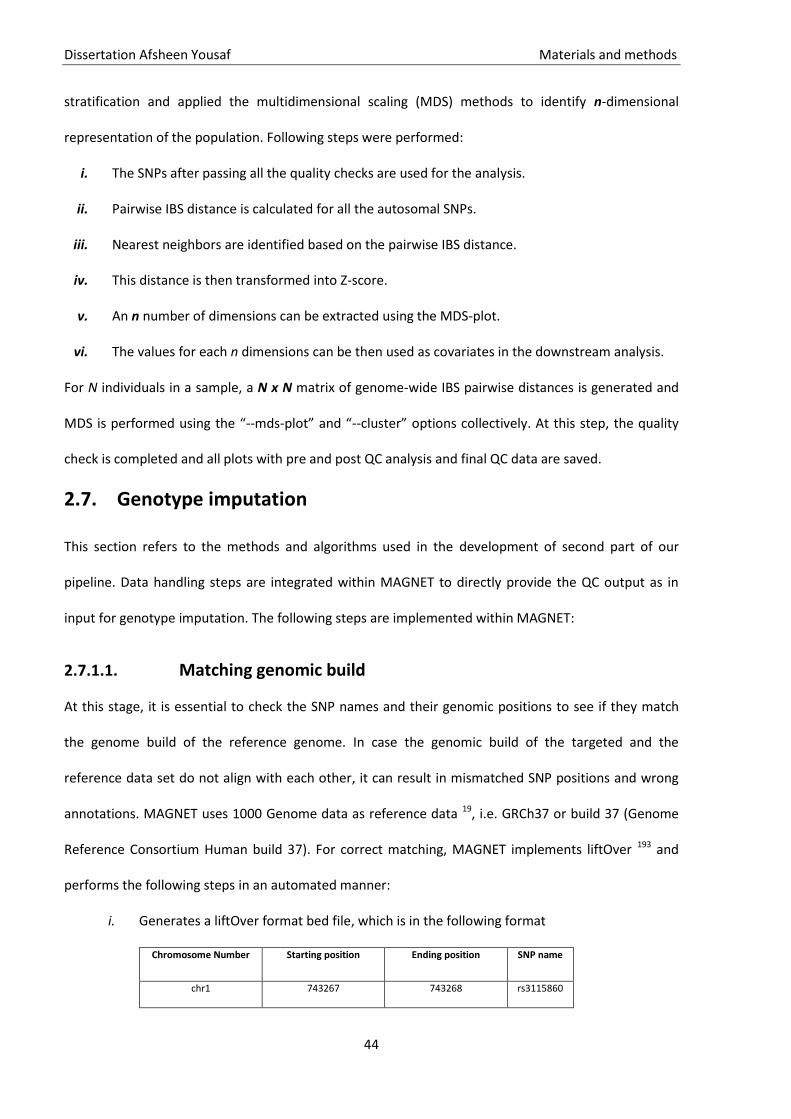
Dissertation Afsheen Yousaf Materials and methods
44
stratification and applied the multidimensional scaling (MDS) methods to identify n-dimensional
representation of the population. Following steps were performed:
i. The SNPs after passing all the quality checks are used for the analysis.
ii. Pairwise IBS distance is calculated for all the autosomal SNPs.
iii. Nearest neighbors are identified based on the pairwise IBS distance.
iv. This distance is then transformed into Z-score.
v. An n number of dimensions can be extracted using the MDS-plot.
vi. The values for each n dimensions can be then used as covariates in the downstream analysis.
For N individuals in a sample, a N x N matrix of genome-wide IBS pairwise distances is generated and
MDS is performed using the “--mds-plot” and “--cluster” options collectively. At this step, the quality
check is completed and all plots with pre and post QC analysis and final QC data are saved.
Genotype imputation 2.7.
This section refers to the methods and algorithms used in the development of second part of our
pipeline. Data handling steps are integrated within MAGNET to directly provide the QC output as in
input for genotype imputation. The following steps are implemented within MAGNET:
2.7.1.1. Matching genomic build
At this stage, it is essential to check the SNP names and their genomic positions to see if they match
the genome build of the reference genome. In case the genomic build of the targeted and the
reference data set do not align with each other, it can result in mismatched SNP positions and wrong
annotations. MAGNET uses 1000 Genome data as reference data 19, i.e. GRCh37 or build 37 (Genome
Reference Consortium Human build 37). For correct matching, MAGNET implements liftOver 193 and
performs the following steps in an automated manner:
i. Generates a liftOver format bed file, which is in the following format
Chromosome Number Starting position Ending position SNP name
chr1 743267 743268 rs3115860

Dissertation Afsheen Yousaf Materials and methods
45
ii. Chooses the chain file (alignment file with chromosome number, chromosome size,
strand, alignment positions of the reference and query sequence) to select for updating
the genome build. Users can select among hg16, hg17, hg18 and hg38 annotation files
depending on the study data (by default hg18). In case the data is already in hg19 format,
the files remain unchanged.
iii. A list of SNPs with an unknown chromosome or position and are not in the hg19 reference
is generated within the pipeline and these SNPs are ultimately removed using PLINK
command “--exclude”.
iv. SNP annotation is then updated by liftOver ensuring that the study and reference genome
build are the same.
v. SNPs that were not updated after liftOver are again removed using the PLINK command
“--exclude” from the PLINK data file.
For the next steps, only affected individuals are considered. By default, we set our pipeline to
distinguish between affected and unaffected individuals using the PLINK coding provided for the
individuals. However, the user is free to choose if all samples are needed for the study. The following
steps will be performed for each chromosome within an automated loop to parallelize the process.
2.7.1.2. Strand checking
The lifted files in the PLINK format will then be provided for strand checking. For a successful and
correct imputation, it is also important that the provided genotype data and the reference alleles are
matched and are annotated based on the same strand. The difference in strands could arise due to
differing genotyping platforms, which may use a forward strand of the human genome assembly, some
use Illuminas’s annotation while some use Affymetrix annotation.
For strand check, we integrated SHAPEIT 145 which highlights and corrects for any strand
inconsistencies. It identifies the SNPs with the possible problem of strand flip and converts the forward
allele to the “+” strand of the human genome reference assembly. It also considers if the alleles are
changed to their complementary alleles (C-G and A-T) based on three criteria: (a) the observed alleles,
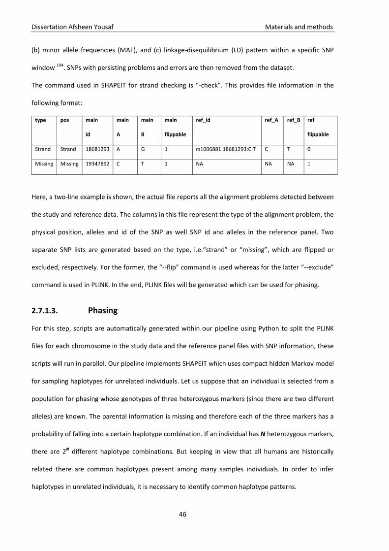
Dissertation Afsheen Yousaf Materials and methods
46
(b) minor allele frequencies (MAF), and (c) linkage-disequilibrium (LD) pattern within a specific SNP
window 194. SNPs with persisting problems and errors are then removed from the dataset.
The command used in SHAPEIT for strand checking is “-check”. This provides file information in the
following format:
type pos main
id
main
A
main
B
main
flippable
ref_id ref_A ref_B ref
flippable
Strand Strand 18681293 A G 1 rs1006881:18681293:C:T C T 0
Missing Missing 19347892 C T 1 NA NA NA 1
Here, a two-line example is shown, the actual file reports all the alignment problems detected between
the study and reference data. The columns in this file represent the type of the alignment problem, the
physical position, alleles and id of the SNP as well SNP id and alleles in the reference panel. Two
separate SNP lists are generated based on the type, i.e.“strand” or “missing”, which are flipped or
excluded, respectively. For the former, the “--flip” command is used whereas for the latter “--exclude”
command is used in PLINK. In the end, PLINK files will be generated which can be used for phasing.
2.7.1.3. Phasing
For this step, scripts are automatically generated within our pipeline using Python to split the PLINK
files for each chromosome in the study data and the reference panel files with SNP information, these
scripts will run in parallel. Our pipeline implements SHAPEIT which uses compact hidden Markov model
for sampling haplotypes for unrelated individuals. Let us suppose that an individual is selected from a
population for phasing whose genotypes of three heterozygous markers (since there are two different
alleles) are known. The parental information is missing and therefore each of the three markers has a
probability of falling into a certain haplotype combination. If an individual has N heterozygous markers,
there are 2N different haplotype combinations. But keeping in view that all humans are historically
related there are common haplotypes present among many samples individuals. In order to infer
haplotypes in unrelated individuals, it is necessary to identify common haplotype patterns.
Dissertation Afsheen Yousaf Materials and methods
47
Let G be the observed genotype and D as the unobserved diplotype of an unrelated individual. A
diplotype here is a pair of haplotypes (h1, h2). Let H denote a set of K haplotypes defined over M
markers. When updating the haplotypes for a given individual, H would be the set of current haplotype
estimates of all other individuals. The total number of markers M are subdivided into non-overlapping
subsets of consecutive markers also termed as “segments” in which the number of distinct haplotypes
in H is limited. The haplotypes of H are split so that there exist ~J haplotypes by segments with J < K.
A graph Hg is built based on these haplotype segments, where edges are the probabilities. At each
marker, there are ∼J nodes, one for each distinct haplotype in the segment in which the marker
resides. The goal is to sample the diplotype for G conditional on the known haplotypes from Hg that is,
by sampling from P(D|G, Hg). The method used in SHAPEIT thus samples pairs of haplotypes from the
probability of h given Hg, i.e. P(h|Hg) that are consistent with G. If G has s heterozygous markers then
the candidate haplotypes would be 2s, where S is used to denote the set of possible haplotypes. This
method scales linearly with the number of haplotypes used in each iteration, i.e. O(MJ). The other
HMM-based methods such as Impute2 and MaCH are O(MJ2)145.
At the end of this step, phased files are generated which are then converted to vcf (variant calling files)
format automatically by our pipeline. This is a standardized format for performing imputation. It is
stored in a compressed manner and can be used for fast data retrieval of genetic variants.
2.7.1.4. Imputation
For performing imputation we integrated a Python script which will automatically create 22 different
jobs, to perform imputation, one for each chromosome. This is one of the main steps of the whole
imputation pipeline. This step was implemented in Minimac3146 because of its reduced computation
time paralleled with a high validity of the imputed variants 147. It is based on the “state space
reduction” of HMM showing haplotype sharing. It looks for similarities among haplotypes in small
genomic segments so that the effective number of states is reduced (see Figure 3).
Consider a chromosome region with M markers and H haplotypes, e.g X1….Xn. The region can be
analysed by breaking it into consecutive genomic blocks based on the markers beginning from the left.
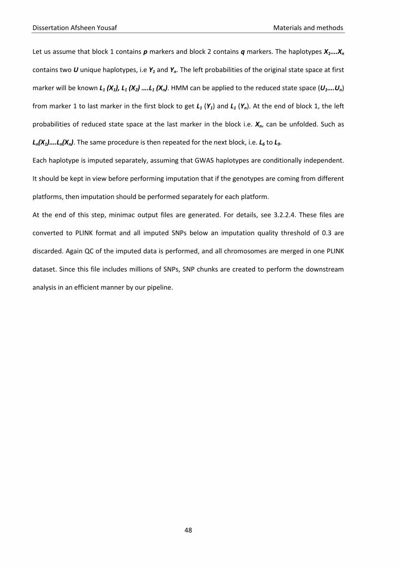
Dissertation Afsheen Yousaf Materials and methods
48
Let us assume that block 1 contains p markers and block 2 contains q markers. The haplotypes X1….Xn
contains two U unique haplotypes, i.e Y1 and Yn. The left probabilities of the original state space at first
marker will be known L1 (X1), L1 (X2) ….L1 (Xn). HMM can be applied to the reduced state space (U1….Un)
from marker 1 to last marker in the first block to get L1 (Y1) and L1 (Yn). At the end of block 1, the left
probabilities of reduced state space at the last marker in the block i.e. Xn, can be unfolded. Such as
Ln(X1)….Ln(Xn). The same procedure is then repeated for the next block, i.e. L6 to L9.
Each haplotype is imputed separately, assuming that GWAS haplotypes are conditionally independent.
It should be kept in view before performing imputation that if the genotypes are coming from different
platforms, then imputation should be performed separately for each platform.
At the end of this step, minimac output files are generated. For details, see 3.2.2.4. These files are
converted to PLINK format and all imputed SNPs below an imputation quality threshold of 0.3 are
discarded. Again QC of the imputed data is performed, and all chromosomes are merged in one PLINK
dataset. Since this file includes millions of SNPs, SNP chunks are created to perform the downstream
analysis in an efficient manner by our pipeline.
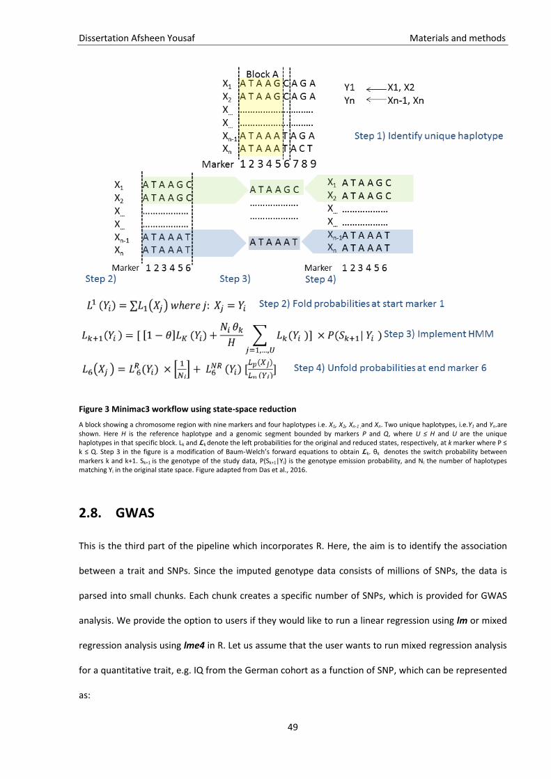
Dissertation Afsheen Yousaf Materials and methods
49
Figure 3 Minimac3 workflow using state-space reduction
A block showing a chromosome region with nine markers and four haplotypes i.e. X1, X2, Xn-1 ,and Xn. Two unique haplotypes, i.e.Y1 and Yn.are shown. Here H is the reference haplotype and a genomic segment bounded by markers P and Q, where U ≤ H and U are the unique haplotypes in that specific block. Lk and 𝓛k denote the left probabilities for the original and reduced states, respectively, at k marker where P ≤ k ≤ Q. Step 3 in the figure is a modification of Baum-Welch’s forward equations to obtain 𝓛k. θk denotes the switch probability between markers k and k+1. Sk+1 is the genotype of the study data, P(Sk+1|Yi) is the genotype emission probability, and Ni the number of haplotypes matching Yi in the original state space. Figure adapted from Das et al., 2016.
GWAS 2.8.
This is the third part of the pipeline which incorporates R. Here, the aim is to identify the association
between a trait and SNPs. Since the imputed genotype data consists of millions of SNPs, the data is
parsed into small chunks. Each chunk creates a specific number of SNPs, which is provided for GWAS
analysis. We provide the option to users if they would like to run a linear regression using lm or mixed
regression analysis using lme4 in R. Let us assume that the user wants to run mixed regression analysis
for a quantitative trait, e.g. IQ from the German cohort as a function of SNP, which can be represented
as:

Dissertation Afsheen Yousaf Materials and methods
50
IQ ~ SNP + ε
Here, “SNP” is a fixed effect and ε is the “error term” that describes the uncertainty in the model due
to the random effects that are difficult to capture completely. Therefore, this error term could be
expanded leaving the fixed part of the model undisturbed. There could be other factors in the model
that could explain the uncertainty in the model, e.g. sex and age. Thus, we add these terms as fixed
effects in the model. So now the model can be written as:
IQ ~ SNP + Sex + Age + ε
Let us further assume that IQ measures are contributed by individuals from different sites, e.g. 60
individuals contributed from Heidelberg, 20 from Freiburg and so on. Hence, each site had multiple IQ
measures. Multiple IQ measures from the same site cannot be regarded as independent from each
other. In order to deal with such situations, we included a random effect in the model that accounts for
“site” from where the individual samples are included. Every site will have different IQ measures that
will affect the measures. By adding random effects, we can get a structure for the error term ε. In this
example, adding a random effect for a site can characterize the distinctive variation, which is due to
individual differences. We can now test for association of IQ with every SNP and controlling for the
effect of recruitment site as an unobserved random intercept since affected individuals’ assessments
might have been different across sites. So the above equation becomes:
IQ ~ SNP + Sex + Age + (1|Site) + ε
The intercept for each subject is different, and 1 stands here for the intercept. This will take into
consideration the non-independence, which occurs from having multiple responses by the same site.
This control captures the between-site differences, thus reducing the overall number of variables while
increasing accuracy and statistical power for the parameters of interest. However, users will have the
option to choose the model accordingly. The scripts were generated in R, and all required packages are
automatically installed upon runtime. In the end, one regression output file is generated for each
chunk. These files contain the effect sizes, nominal and adjusted p-values along with other information
Dissertation Afsheen Yousaf Materials and methods
51
(see 3.2.3.4). All files are then merged. A text file containing only the SNP id and the p-value is
extracted within the pipeline for further analysis.
Gene-based analysis 2.9.
In this part, we implemented the gene-based analysis and directly take the text file with SNP and p-
value information as input. The output of GWAS will be provided as input for gene-based analysis after
arranging the file in the format for performing SNP-wise gene-based analysis. This analysis is
performed using MAGMA.
Firstly, the SNPs are mapped to the corresponding gene, based on NCBI GRCh37/hg19 annotation
within a window of 5 kilobases (kb) up and downstream of the respective coding sequence. However,
we provided users the option to define a window-size.
It secondly analyses the individual SNPs in a gene and adds their respective p-value into a gene test-
statistic. We selected the mean of the χ2 statistic for the SNPs in a gene. The observed gene-statistic is
computed from the regression output, i.e. SNP and p-values taking into consideration, only the SNPs,
which are in the reference dataset. In our case, it is the 1000 Genomes dataset which is used to
estimate the SNP statistic correlation matrix “R”.
A gene p-value is calculated by using a known approximation of the sampling distribution. For
computing the approximate sampling distribution p-values, the correlation matrix “R” is required for
SNP statistics. The correlations between the gene model sum of squares (SSM) values of the regression
model are taken into account, which describes how well a regression model represents the modeled
data. For single SNPs, a square of the correlation between the SNP genotype values is generated.
In general, the approximate sampling distribution is based on the basic properties of the multivariate
normal distribution. Assuming under a null hypothesis of no association, the individual SNP Z-values zi
have a standard normal distribution, and therefore their joint distribution can be assumed to be a
multivariate normal distribution with a mean of 0 and covariance equal to the correlation matrix R.
Dissertation Afsheen Yousaf Materials and methods
52
Besides a normal p-value, a permutation-based p-value is also calculated for all gene test-statistics. We
selected adaptive permutations, which means that the number of permutation varies per gene. The
genes are coded as Entrez gene, which are unique integers based on the gene-specific database
(www.ncbi.nlm.nih.gov/gene) at the NCBI (National Center for Biotechnology Information).
Initially, for every gene 1,000 permutations are generated. MAGMA checks the number of P
permutations with a gene test-statistic greater than the observed gene statistic. In case this value is
greater than the pre-specified threshold Pthresh, the empirical p-value is calculated. In this way, an
empirical p-value is calculated for all the genes.
In other cases, if the value is smaller, the number of permutations is increased to 5,000 and P is
checked again, which will continue for checking at 10,000, 50,000 and so on until P > Pthresh or the
maximum number of permutations is reached, i.e. 1,000,000. At the end of the analysis, a file with
significant genes along with a system code, i.e. “L” for Entrez gene ids is created for performing gene
ontology analysis.
Gene Ontology analysis 2.10.
In this step, we integrated Gene Ontology (GO) analysis. The significant gene list from the previous
analysis, will serve as input for identifying the underlying biological pathways. Thus, the input file is (i)
the list of all significant gene IDs (here, Entrez gene ids) named “input file”, (ii) a file containing all
genes tested in MAGMA named as the “denominator file”, which is in the same format as the input
file, which serve as the background gene list to test for enrichment.
Gene ontology ORA (Over-representation analysis) is a method to test if the set of biologically related
terms occur more often than would be expected by chance in the dataset. This analysis provides
information about the ontology id, the number of genes associated with the ontology id, Z-score,
permuted and adjusted p-values. The gene lists are tested to avoid redundancy by using a robust
pruning method to provide a set of non-overlapping terms. The statistics is based on Z-scores, p-values
and gene counts, and look for unique branch paths from the overall ontology tree structure. This is

Dissertation Afsheen Yousaf Materials and methods
53
performed via pruning to attain the node which has the largest Z-score in comparison to its
corresponding child and parent nodes.
To identify functional profiles and underlying pathways of the genetic variants, we performed gene-
based tests for GO-term and pathway enrichment. This step is performed using GO-Elite 162 and the R
package kegga for identifying associated KEGG pathways. Z-scores are calculated, using the normal
approximation to the hypergeometric distribution along with a permutation or a Fisher's exact test
p-value. GO-Elite ranks each analysed term according to the Z-score. The method is detailed as
follows:
A Z-score and permutation or Fisher’s exact test p-value are calculated to look for the over-
representation of genes within specific ontology terms and pathways.
( ) ( )
( )
The probability of observed gene IDs (observed probability) from the significant gene list is subtracted
from the probability of combined total gene IDs of all the MAGMA genes (expected probability) and
divided by the standard deviation of the observed gene IDs (Observed probability). The statistics can
be further explained as the following equation:
[
]
√ [
][ [
]][
]
,
where
n = Total IDs associated with a biological term (denominator list)
r = Input IDs associated with a biological term (input list)
N = Denominator IDs examined (denominator list)
R = Total Input IDs (input list)
A Fisher’s exact test is calculated by creating a 2x2 contingency table. The table will consist of (a) the
number of input IDs within a biological term, i.e. “r”, (b) a number of non-input IDs in a biological term
Dissertation Afsheen Yousaf Materials and methods
54
(n-r), (c) a number of input IDs excluded from that term (R) and (d) the number of non-input IDs
excluded from that term (N-R-n-r).
In order to reduce the possibility of chance findings, permutation analysis is performed. A random
number of source IDs are selected from the “input file” and “denominator file” in an equal amount.
Again, Z scores are recalculated for all terms “X” times, where X is a user-defined value. By default, we
provide an option of X= 2000. Now, the likelihood of a Z-score occurring by chance is calculated as the
number of times a permutation Z-score is greater than or equal to the original Z-score divided by X.
Further, a false-discovery rate (FDR) p-value is calculated from the Fisher’s exact test or permutation
p-value based on the Benjamini-Hochberg (BH) correction (see Appendix).
The output file contains the name of the ontology, number of genes in the input and matching
pathway/GO-term, gene names involved in the pathway, a Z-score, a permuted and adjusted p-value.
Brain enrichment analysis 2.11.
The last step of the pipeline performs brain enrichment analysis. We integrated the Kang et al. 48 brain
transcriptome data set within the pipeline. This will assist in gathering information on the brain-specific
effects of associated genes at 16 different brain regions i.e. Orbital prefrontal cortex (OFC),
Dorsolateral prefrontal cortex (DFC), Ventrolateral prefrontal cortex (VFC), Medial prefrontal cortex
(MFC), Primary motor cortex (M1C), Primary somatosensory cortex (S1C), Posterior inferior parietal
cortex (IPC), Primary auditory cortex (A1C), Posterior superior temporal cortex (STC), Inferior temporal
cortex (ITC), Primary visual cortex (V1C), Hippocampus (HIP), Amygdala (AMY), Striatum (STR),
Mediodorsal nucleus of the thalamus (MD), and Cerebellar cortex (CBC). Gene expression at these
brain regions can be seen within a time frame, ranging from embryonic development to late adulthood
of males and females. This dataset consists of 1,340 tissue samples collected from one or both
hemispheres of 57 postmortem human brains. Co-expression pattern of genes within this dataset is
distinguished into 29 co-regulated gene modules 4. Enrichment analysis is implemented using Fisher’s
exact test. Two-dimensional heatmaps with brain anatomical structures over time were plotted using
Dissertation Afsheen Yousaf Materials and methods
55
the R package CerebroViz 49 to visualize the eigengene (first principal component) values for each
module. Moreover, we generated gene networks of the modules, which highlighted the overlapping
genes from each subdomain. Gene networks were plotted using the R package igraph 50. For details on
the output, please see 3.2.4.4.
We discussed till here all the parts of the pipeline with respect to the thresholds and methods
implemented. Further, we used additional methods that are currently not part of the pipeline but were
performed to answer the biological question using the combined ASD cohort (AGP and German). The
PLINK files from the two separate cohorts were merged using the “--merge” command in PLINK.
III. Additional data analysis
Genetic correlation 2.12.
Genetic correlation analysis depicts the genetic relationship between two traits. This analysis will
provide an understanding if the genetic variants on the two traits are shared, as well as if the alleles
that affect one trait might have an effect on a second trait.
The genetic correlation is defined as follows:
( )
√ ( ) ( ) ,
where
( ) is the additive genetic variance of trait i , and
( ) is the additive genetic covariance between the traits.
For performing this analysis, the PLINK files were first converted into GRM (genetic relationship matrix)
format. We used bivariate GCTA–GREML from the GCTA tool 195 to estimate the genetic correlation
based on the combined (AGP and German cohorts) cohort containing the phenotypic and genotypic
information from unrelated individuals. The GCTA bivariate method is an extension of the univariate
model which relates the pairwise genetic similarity matrix to a phenotypic covariance matrix between
Dissertation Afsheen Yousaf Materials and methods
56
the first trait of interest with the second trait of interest and allows for correlated residuals. Before
calculating rg, GCTA estimates the genetic relationship matrix (GRM) between unrelated individuals
from the SNPs, which can be estimated as follows:
∑
( )( )
( )
,
where
xij is the number of copies of the reference allele for the ith SNP of the jth individual,
j and k are individuals for which the genetic relationship between two individuals will be calculated,
pi is the reference allele, and
N is the number of SNPs.
In this way, iteratively one individual of a pair is excluded, whose relationship is greater than a
specified threshold. Genetic correlations are then calculated based on the GRM.
SNP-based heritability analysis 2.13.
This analysis is performed to estimate the phenotypic variance explained by all SNPs in a GWAS based
on unrelated individuals. The heritability analysis was also performed in GCTA using the combined ASD
data in GRM format. SNP-based heritability (h2SNP) is calculated to estimate the total variance of a
phenotype, which can be explained by all SNPs. We calculated the SNP-based heritability (h2SNP) based
on unrelated individuals since this avoids the bias in estimates, which occur due to the effect of
common environment (dominance/epistasis) of the related individuals, e.g. siblings or twins.
Moreover, to attain the minimum sample size requirements, we performed the analysis in the
combined cohort. SNP-based heritability for each quantitative trait (subdomain) was estimated as
follows:
( ) ,
Dissertation Afsheen Yousaf Materials and methods
57
where
is the genetic variance, and
is the residual variance.
These variances are calculated using REML from the GRM as shown in the previous section.
The variance explained by genome-wide SNPs (i.e. variance explained by all the causal variants) is
estimated based on two steps: (i) A GRM calculated for all SNPs. This is an NxN matrix where each
element represents the genetic similarity of two individuals. (ii) REML analysis where GRM is used as a
predictor in the mixed linear model with the individual subdomain as the dependent variable. This
analysis is performed in GCTA 195.
Polygenic risk scores (PRS) 2.14.
To identify the level of shared genetic etiology between ASD and the quantitative traits, we performed
a polygenic risk score-based analysis in the combined cohort (i.e. AGP and German cohort) using PRSice
which requires the GWAS output from individual subdomains 196.
In general, PRS is an estimate of an individual’s predisposition to a trait. It is determined by the sum of
their genome-wide genotypes and weighted based on the corresponding genotype effect sizes which
are collected from the GWAS summary statistics.
For this analysis two datasets are required as input:
i. Base dataset: A reference GWAS summary statistics data. We used the PGC-ASD GWAS data
consisting of 5,305 ASD cases and 5,305 controls. Data is publically available:
http://www.med.unc.edu/pgc/downloads.
ii. Target dataset: GWAS summary statistics of the target dataset. In our study, we have six
different GWAS summary statistics for each of the quantitative traits (subdomains), i.e. JA, SI,
PI, NVC, RB, and RI.

Dissertation Afsheen Yousaf Materials and methods
58
iii. To avoid any bias in the results, we made sure that the individuals of the PGC-ASD GWAS are
not part of our consortium as the inclusion of related individuals can result in inflation of
output.
iv. We only selected the SNPs, which were overlapping in the base and target datasets.
v. Clumping of SNPs was performed using PLINK to attain SNPs that are largely independent of
each other. We selected a significance threshold for index SNPs of 0.001; the secondary
significance threshold for clumped SNPs was 0.01. The LD threshold was 0.1 and the physical
distance threshold for clumping was 250 kb. This generated a list of clumped SNPs.
vi. Genomic profile scores will be generated in the target dataset, e.g. the sum of risk alleles
weighted by base dataset effect size (betas, log odds ratio, etc.). It is possible that the causal
SNPs in GWAS could not attain a significant p-value, therefore, PRS are calculated at a set of
seven broad thresholds that are <0.001, 0.05, 0.1, 0.2, 0.3, 0.4, 0.5.
vii. Based on the above mentioned seven P thresholds, polygenic risk scores are generated based
on all SNPs that were associated with the PGC-ASD data (base data).
viii. PRSice also calculated the P of shared genetic etiology, i.e. the extent to which the combined
SNPs from each of the seven P-value threshold linked polygenic risk scores for ASD predict
each of the six quantitative subdomains-between the base ASD phenotype and target
phenotypes, i.e. the total autistic score as well as the score for each of the subdomain.
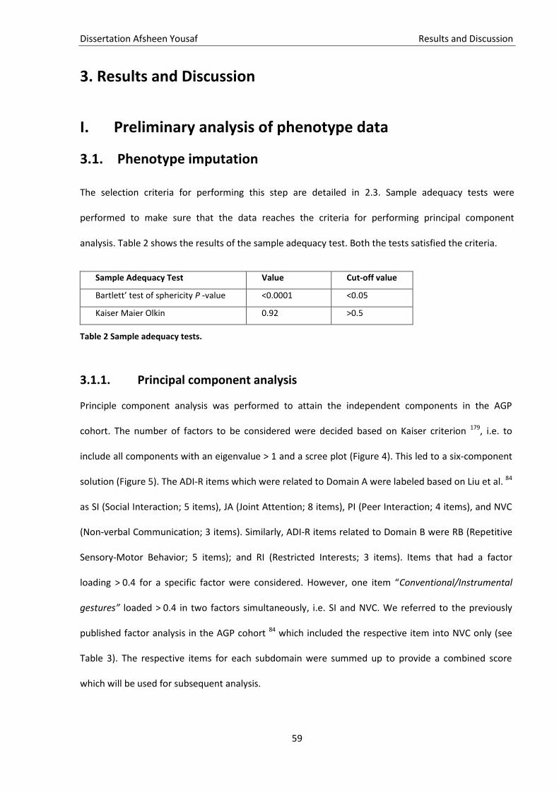
Dissertation Afsheen Yousaf Results and Discussion
59
3. Results and Discussion
I. Preliminary analysis of phenotype data
Phenotype imputation 3.1.
The selection criteria for performing this step are detailed in 2.3. Sample adequacy tests were
performed to make sure that the data reaches the criteria for performing principal component
analysis. Table 2 shows the results of the sample adequacy test. Both the tests satisfied the criteria.
Sample Adequacy Test Value Cut-off value
Bartlett’ test of sphericity P -value <0.0001 <0.05
Kaiser Maier Olkin 0.92 >0.5
Table 2 Sample adequacy tests.
3.1.1. Principal component analysis
Principle component analysis was performed to attain the independent components in the AGP
cohort. The number of factors to be considered were decided based on Kaiser criterion 179, i.e. to
include all components with an eigenvalue > 1 and a scree plot (Figure 4). This led to a six-component
solution (Figure 5). The ADI-R items which were related to Domain A were labeled based on Liu et al. 84
as SI (Social Interaction; 5 items), JA (Joint Attention; 8 items), PI (Peer Interaction; 4 items), and NVC
(Non-verbal Communication; 3 items). Similarly, ADI-R items related to Domain B were RB (Repetitive
Sensory-Motor Behavior; 5 items); and RI (Restricted Interests; 3 items). Items that had a factor
loading > 0.4 for a specific factor were considered. However, one item “Conventional/Instrumental
gestures” loaded > 0.4 in two factors simultaneously, i.e. SI and NVC. We referred to the previously
published factor analysis in the AGP cohort 84 which included the respective item into NVC only (see
Table 3). The respective items for each subdomain were summed up to provide a combined score
which will be used for subsequent analysis.
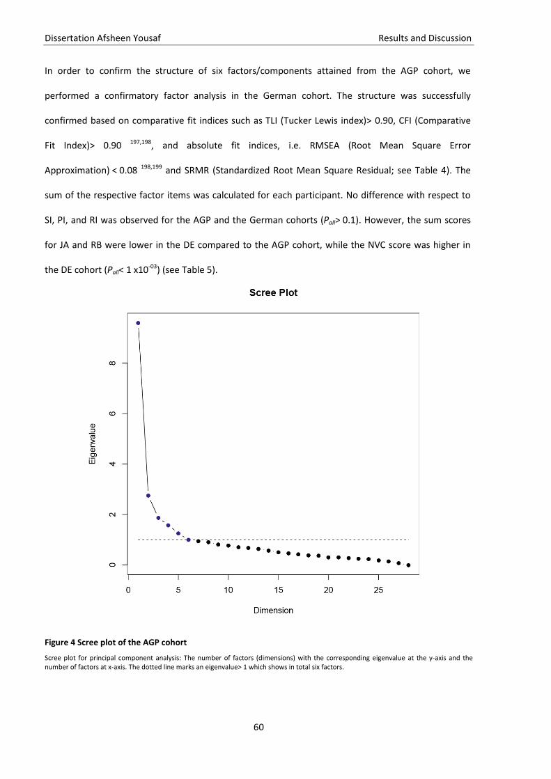
Dissertation Afsheen Yousaf Results and Discussion
60
In order to confirm the structure of six factors/components attained from the AGP cohort, we
performed a confirmatory factor analysis in the German cohort. The structure was successfully
confirmed based on comparative fit indices such as TLI (Tucker Lewis index)> 0.90, CFI (Comparative
Fit Index)> 0.90 197,198, and absolute fit indices, i.e. RMSEA (Root Mean Square Error
Approximation) < 0.08 198,199 and SRMR (Standardized Root Mean Square Residual; see Table 4). The
sum of the respective factor items was calculated for each participant. No difference with respect to
SI, PI, and RI was observed for the AGP and the German cohorts (Pall> 0.1). However, the sum scores
for JA and RB were lower in the DE compared to the AGP cohort, while the NVC score was higher in
the DE cohort (Pall< 1 x10-03) (see Table 5).
Figure 4 Scree plot of the AGP cohort
Scree plot for principal component analysis: The number of factors (dimensions) with the corresponding eigenvalue at the y-axis and the number of factors at x-axis. The dotted line marks an eigenvalue> 1 which shows in total six factors.

Dissertation Afsheen Yousaf Results and Discussion
61
Figure 5 PCA based subdomains of the 28 ADI-R items
The color bar and size of the dots represent the intensity of correlation. Abbreviations: JA: Joint attention, SI: Social interaction, PI: Peer Interaction, NVC: Non-verbal communication, RB: Repetitive Sensory-Motor Behavior, RI: Restricted interests.
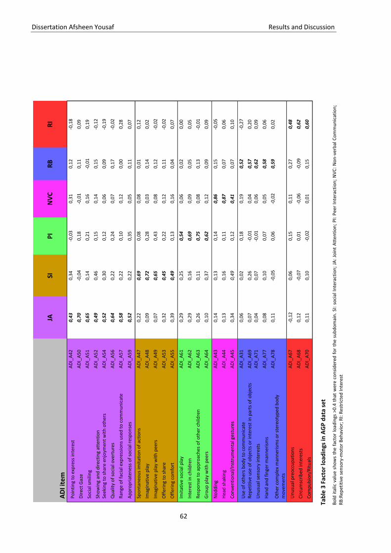
Dissertation Afsheen Yousaf Results and Discussion
62
AD
I ite
m
JA
SI
PI
NV
C
RB
R
I
Po
inti
ng
to e
xpre
ss in
tere
st
AD
I_A
42
0,4
3
0,3
4 -0
,03
0,3
1 0
,12
-0,1
8
Dir
ect
Gaz
e
AD
I_A
50
0,7
0
-0,0
4 0
,18
-0,0
1 0
,11
0,0
9
Soci
al s
mili
ng
AD
I_A
51
0,6
5
0,1
4 0
,21
0,1
6 -0
,01
0,1
9
Sho
win
g an
d d
irec
tin
g at
ten
tio
n
AD
I_A
52
0,4
9
0,4
6 0
,15
0,1
4 0
,15
-0,1
2
Seek
ing
to s
har
e en
joym
ent
wit
h o
ther
s A
DI_
A5
4 0
,52
0
,30
0,1
2 0
,06
0,0
9 -0
,19
Qu
alit
y o
f so
cial
ove
rtu
res
AD
I_A
56
0,6
4
0,2
2 0
,24
0,0
7 0
,17
-0,0
2
Ran
ge o
f fa
cial
exp
ress
ion
s u
sed
to
co
mm
un
icat
e A
DI_
A5
7 0
,58
0
,22
0,1
0 0
,12
0,0
0 0
,28
Ap
pro
pri
aten
ess
of
soci
al r
esp
on
ses
AD
I_A
59
0,5
2
0,2
2 0
,35
0,0
5 0
,11
0,0
7
Spo
nta
neo
us
imit
atio
n o
f ac
tio
ns
AD
I_A
47
0,2
2 0
,69
0
,08
0,0
8 0
,01
0,1
2
Imag
inat
ive
pla
y A
DI_
A4
8 0
,09
0,7
2
0,2
8 0
,03
0,1
4 0
,02
Imag
inat
ive
pla
y w
ith
pee
rs
AD
I_A
49
0,0
7 0
,65
0
,43
0,0
8 0
,12
-0,0
2
Off
erin
g to
sh
are
A
DI_
A5
3 0
,32
0,4
5
0,2
2 0
,12
0,1
1 -0
,02
Off
erin
g co
mfo
rt
AD
I_A
55
0,3
9 0
,49
0
,13
0,1
6 0
,04
0,0
7
Imit
ativ
e so
cial
pla
y A
DI_
A6
1 0
,29
0,2
5 0
,54
0
,06
0,0
2 0
,00
Inte
rest
in c
hild
ren
A
DI_
A6
2 0
,29
0,1
6 0
,69
0
,09
0,0
5 0
,05
Res
po
nse
to
ap
pro
ach
es o
f o
ther
ch
ildre
n
AD
I_A
63
0,2
6 0
,11
0,7
5
0,0
8 0
,13
-0,0
1
Gro
up
pla
y w
ith
pee
rs
AD
I_A
64
0,1
0 0
,37
0,6
2
0,1
2 0
,09
0,0
9
No
dd
ing
AD
I_A
43
0,1
4 0
,13
0,1
4 0
,86
0
,15
-0,0
5
Hea
d s
hak
ing
AD
I_A
44
0,1
3 0
,16
0,1
1 0
,87
0
,07
0,0
6
Co
nve
nti
on
al/I
nst
rum
enta
l ges
ture
s A
DI_
A4
5 0
,34
0,4
9 0
,12
0,4
1
0,0
7 0
,10
Use
of
oth
ers
bo
dy
to c
om
mu
nic
ate
A
DI_
A3
1 0
,06
0,0
2 0
,18
0,1
9 0
,52
-0
,27
Rep
etit
ive
use
of
ob
ject
s o
r in
tere
st in
par
ts o
f o
bje
cts
AD
I_A
69
0,0
7 0
,26
-0,0
1 0
,04
0,5
7
0,2
0
Un
usu
al s
enso
ry in
tere
sts
AD
I_A
71
0,0
4 0
,07
-0,0
1 0
,06
0,6
2
0,0
9
Han
d a
nd
fin
ger
man
ner
ism
s A
DI_
A7
7 0
,08
0,1
0 0
,07
0,0
5 0
,58
0
,06
Oth
er c
om
ple
x m
ann
eris
ms
or
ster
eoty
ped
bo
dy
mo
vem
ents
AD
I_A
78
0,1
1 -0
,05
0,0
6 -0
,02
0,5
9
0,0
2
Un
usu
al p
reo
ccu
pat
ion
s A
DI_
A6
7 -0
,12
0,0
6 0
,15
0,1
1 0
,27
0,4
8
Cir
cum
scri
bed
inte
rest
s A
DI_
A6
8 0
,12
-0,0
7 0
,01
-0,0
6 -0
,09
0,6
2
Co
mp
uls
ion
/Rit
ual
s A
DI_
A7
0 0
,11
0,1
0 -0
,02
0,0
1 0
,15
0,6
0
Tab
le 3
Fac
tor
load
ings
in A
GP
dat
a se
t
Bo
ld i
talic
val
ue
sho
ws
the
fac
tor
load
ings
>0
.4 t
hat
wer
e co
nsi
der
ed f
or
the
sub
do
mai
n.
SI:
soci
al I
nte
ract
ion
; JA
: Jo
int
Att
enti
on
; P
I: P
eer
Inte
ract
ion
; N
VC
: N
on
-ver
bal
Co
mm
un
icat
ion
; R
B:R
epet
itiv
e s
enso
ry-m
oto
r B
ehav
ior;
RI:
Res
tric
ted
Inte
rest
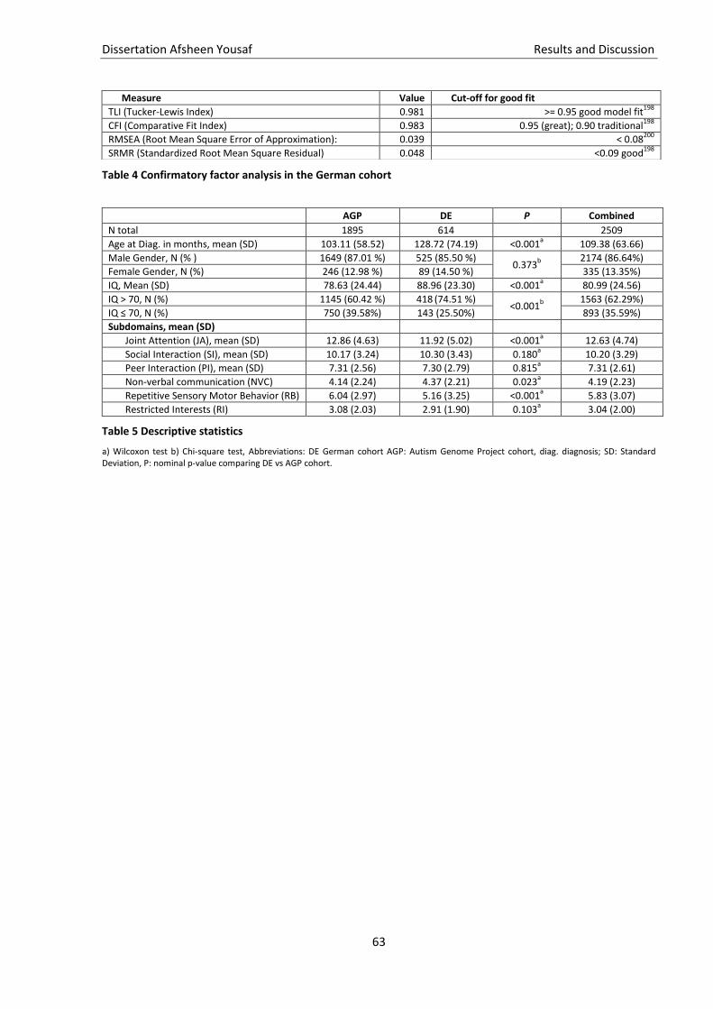
Dissertation Afsheen Yousaf Results and Discussion
63
Table 4 Confirmatory factor analysis in the German cohort
AGP DE P Combined
N total 1895 614 2509
Age at Diag. in months, mean (SD) 103.11 (58.52) 128.72 (74.19) <0.001a
109.38 (63.66)
Male Gender, N (% ) 1649 (87.01 %) 525 (85.50 %) 0.373
b 2174 (86.64%)
Female Gender, N (%) 246 (12.98 %) 89 (14.50 %) 335 (13.35%)
IQ, Mean (SD) 78.63 (24.44) 88.96 (23.30) <0.001a
80.99 (24.56)
IQ > 70, N (%) 1145 (60.42 %) 418 (74.51 %)
<0.001b 1563 (62.29%)
IQ ≤ 70, N (%) 750 (39.58%) 143 (25.50%) 893 (35.59%)
Subdomains, mean (SD)
Joint Attention (JA), mean (SD) 12.86 (4.63) 11.92 (5.02) <0.001a
12.63 (4.74)
Social Interaction (SI), mean (SD) 10.17 (3.24) 10.30 (3.43) 0.180a
10.20 (3.29)
Peer Interaction (PI), mean (SD) 7.31 (2.56) 7.30 (2.79) 0.815a 7.31 (2.61)
Non-verbal communication (NVC) 4.14 (2.24) 4.37 (2.21) 0.023a
4.19 (2.23)
Repetitive Sensory Motor Behavior (RB) 6.04 (2.97) 5.16 (3.25) <0.001a
5.83 (3.07)
Restricted Interests (RI) 3.08 (2.03) 2.91 (1.90) 0.103a
3.04 (2.00)
Table 5 Descriptive statistics
a) Wilcoxon test b) Chi-square test, Abbreviations: DE German cohort AGP: Autism Genome Project cohort, diag. diagnosis; SD: Standard Deviation, P: nominal p-value comparing DE vs AGP cohort.
Measure Value Cut-off for good fit
TLI (Tucker-Lewis Index) 0.981 >= 0.95 good model fit198
CFI (Comparative Fit Index) 0.983 0.95 (great); 0.90 traditional198
RMSEA (Root Mean Square Error of Approximation): 0.039 < 0.08200
SRMR (Standardized Root Mean Square Residual) 0.048 <0.09 good198
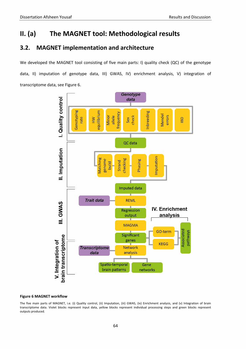
Dissertation Afsheen Yousaf Results and Discussion
64
II. (a) The MAGNET tool: Methodological results
MAGNET implementation and architecture 3.2.
We developed the MAGNET tool consisting of five main parts: I) quality check (QC) of the genotype
data, II) imputation of genotype data, III) GWAS, IV) enrichment analysis, V) integration of
transcriptome data, see Figure 6.
Figure 6 MAGNET workflow
The five main parts of MAGNET, i.e. (i) Quality control, (ii) Imputation, (iii) GWAS, (iv) Enrichment analysis, and (v) Integration of brain transcriptome data. Violet blocks represent input data, yellow blocks represent individual processing steps and green blocks represent outputs produced.
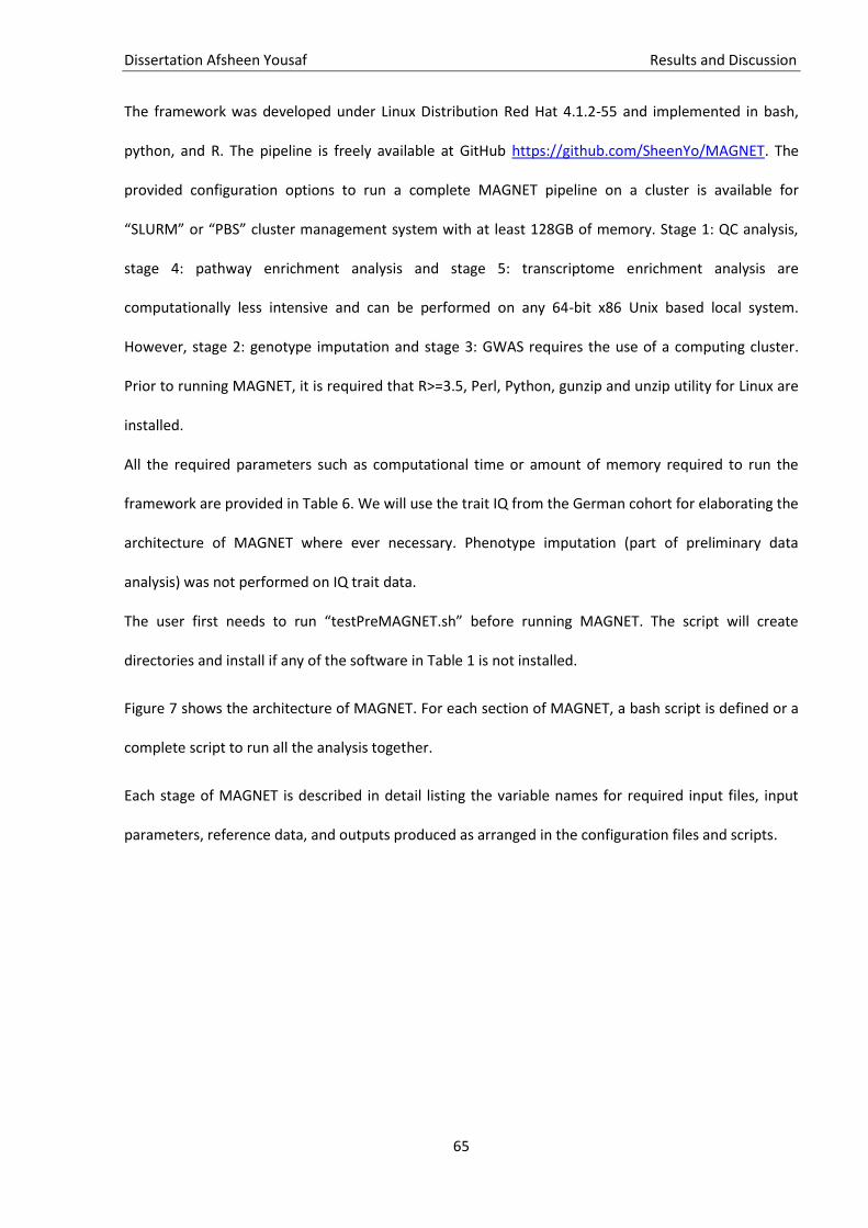
Dissertation Afsheen Yousaf Results and Discussion
65
The framework was developed under Linux Distribution Red Hat 4.1.2-55 and implemented in bash,
python, and R. The pipeline is freely available at GitHub https://github.com/SheenYo/MAGNET. The
provided configuration options to run a complete MAGNET pipeline on a cluster is available for
“SLURM” or “PBS” cluster management system with at least 128GB of memory. Stage 1: QC analysis,
stage 4: pathway enrichment analysis and stage 5: transcriptome enrichment analysis are
computationally less intensive and can be performed on any 64-bit x86 Unix based local system.
However, stage 2: genotype imputation and stage 3: GWAS requires the use of a computing cluster.
Prior to running MAGNET, it is required that R>=3.5, Perl, Python, gunzip and unzip utility for Linux are
installed.
All the required parameters such as computational time or amount of memory required to run the
framework are provided in Table 6. We will use the trait IQ from the German cohort for elaborating the
architecture of MAGNET where ever necessary. Phenotype imputation (part of preliminary data
analysis) was not performed on IQ trait data.
The user first needs to run “testPreMAGNET.sh” before running MAGNET. The script will create
directories and install if any of the software in Table 1 is not installed.
Figure 7 shows the architecture of MAGNET. For each section of MAGNET, a bash script is defined or a
complete script to run all the analysis together.
Each stage of MAGNET is described in detail listing the variable names for required input files, input
parameters, reference data, and outputs produced as arranged in the configuration files and scripts.
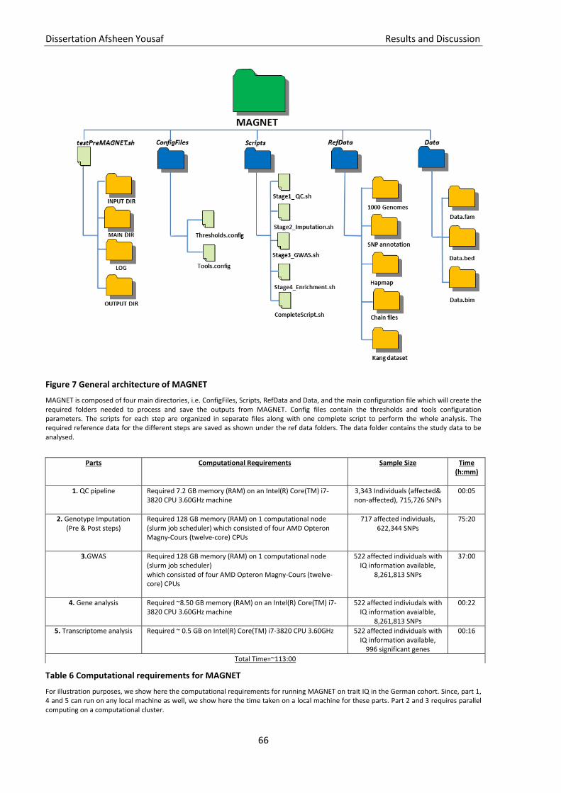
Dissertation Afsheen Yousaf Results and Discussion
66
Figure 7 General architecture of MAGNET
MAGNET is composed of four main directories, i.e. ConfigFiles, Scripts, RefData and Data, and the main configuration file which will create the required folders needed to process and save the outputs from MAGNET. Config files contain the thresholds and tools configuration parameters. The scripts for each step are organized in separate files along with one complete script to perform the whole analysis. The required reference data for the different steps are saved as shown under the ref data folders. The data folder contains the study data to be analysed.
Table 6 Computational requirements for MAGNET
For illustration purposes, we show here the computational requirements for running MAGNET on trait IQ in the German cohort. Since, part 1, 4 and 5 can run on any local machine as well, we show here the time taken on a local machine for these parts. Part 2 and 3 requires parallel computing on a computational cluster.
Parts Computational Requirements Sample Size Time (h:mm)
1. QC pipeline
Required 7.2 GB memory (RAM) on an Intel(R) Core(TM) i7-3820 CPU 3.60GHz machine
3,343 Individuals (affected& non-affected), 715,726 SNPs
00:05
2. Genotype Imputation (Pre & Post steps)
Required 128 GB memory (RAM) on 1 computational node (slurm job scheduler) which consisted of four AMD Opteron Magny-Cours (twelve-core) CPUs
717 affected individuals, 622,344 SNPs
75:20
3.GWAS
Required 128 GB memory (RAM) on 1 computational node (slurm job scheduler) which consisted of four AMD Opteron Magny-Cours (twelve-core) CPUs
522 affected individuals with IQ information available,
8,261,813 SNPs
37:00
4. Gene analysis
Required ~8.50 GB memory (RAM) on an Intel(R) Core(TM) i7-3820 CPU 3.60GHz machine
522 affected indiviudals with IQ information avaialble,
8,261,813 SNPs
00:22
5. Transcriptome analysis
Required ~ 0.5 GB on Intel(R) Core(TM) i7-3820 CPU 3.60GHz
522 affected individuals with IQ information available,
996 significant genes
00:16
Total Time=~113:00
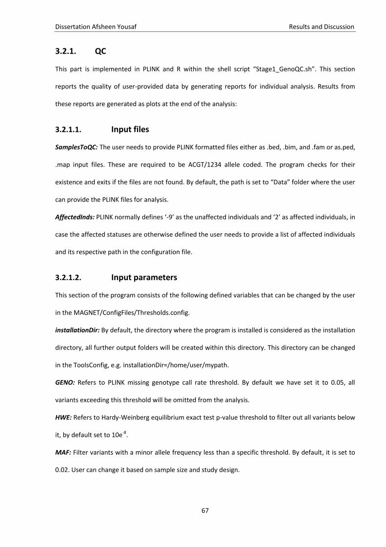
Dissertation Afsheen Yousaf Results and Discussion
67
3.2.1. QC
This part is implemented in PLINK and R within the shell script “Stage1_GenoQC.sh”. This section
reports the quality of user-provided data by generating reports for individual analysis. Results from
these reports are generated as plots at the end of the analysis:
3.2.1.1. Input files
SamplesToQC: The user needs to provide PLINK formatted files either as .bed, .bim, and .fam or as.ped,
.map input files. These are required to be ACGT/1234 allele coded. The program checks for their
existence and exits if the files are not found. By default, the path is set to “Data” folder where the user
can provide the PLINK files for analysis.
AffectedInds: PLINK normally defines ‘-9’ as the unaffected individuals and ‘2’ as affected individuals, in
case the affected statuses are otherwise defined the user needs to provide a list of affected individuals
and its respective path in the configuration file.
3.2.1.2. Input parameters
This section of the program consists of the following defined variables that can be changed by the user
in the MAGNET/ConfigFiles/Thresholds.config.
installationDir: By default, the directory where the program is installed is considered as the installation
directory, all further output folders will be created within this directory. This directory can be changed
in the ToolsConfig, e.g. installationDir=/home/user/mypath.
GENO: Refers to PLINK missing genotype call rate threshold. By default we have set it to 0.05, all
variants exceeding this threshold will be omitted from the analysis.
HWE: Refers to Hardy-Weinberg equilibrium exact test p-value threshold to filter out all variants below
it, by default set to 10e-8.
MAF: Filter variants with a minor allele frequency less than a specific threshold. By default, it is set to
0.02. User can change it based on sample size and study design.
Dissertation Afsheen Yousaf Results and Discussion
68
MIND: Excludes all samples which have missing genotype data greater than a specific threshold, here it
is by default set as 0.05.
MEFam and MESNP: These options are used for family-based data only. Filters individuals and/or
markers based on the Mendel error rate.
MEFam: By default discards all the families with more than 1% Mendel errors (considering all SNPs).
MESNP: By default discards all the SNPs with more than 10% Mendel error rate based on the number
of trios.
3.2.1.3. Reference files
For this stage only HapMap data is required:
Hapmapfile: Hapmap genotype file for generating ethnicity plots
3.2.1.4. Output
QC1_report.imiss: A list reporting sample-based missingness, where F_MISS column details the missing
call rate.
QC1_report.lmiss: A list reporting variant based missingness, where F_MISS column details the missing
call rate.
PreQC_hardy.hwe: A statistic generated showing the Hardy-Weinberg exact test with p-values.
PreQC_AlleleFreq.frq: Lists all the SNPs with minor allele frequencies.
PreQC_Inbreeding.het: Generates the inbreeding coefficient estimates.
QC2_Sexcheck.sexcheck: Reports the individuals with mismatched gender.
FinalQC_Study: In the end, the user gets a clean quality checked PLINK data file, which will be directly
incorporated for the next section. Altogether 9 graphs are produced at the end of QC, as an example
six different QC output plots of IQ trait from the German cohort are shown in Figure 8.
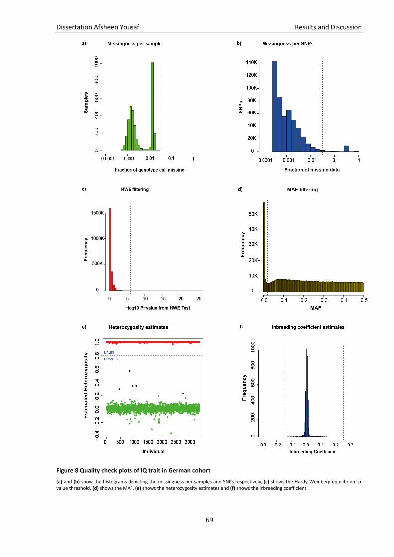
Dissertation Afsheen Yousaf Results and Discussion
69
Figure 8 Quality check plots of IQ trait in German cohort
(a) and (b) show the histograms depicting the missingness per samples and SNPs respectively, (c) shows the Hardy-Weinberg equilibrium p-value threshold, (d) shows the MAF, (e) shows the heterozygosity estimates and (f) shows the inbreeding coefficient
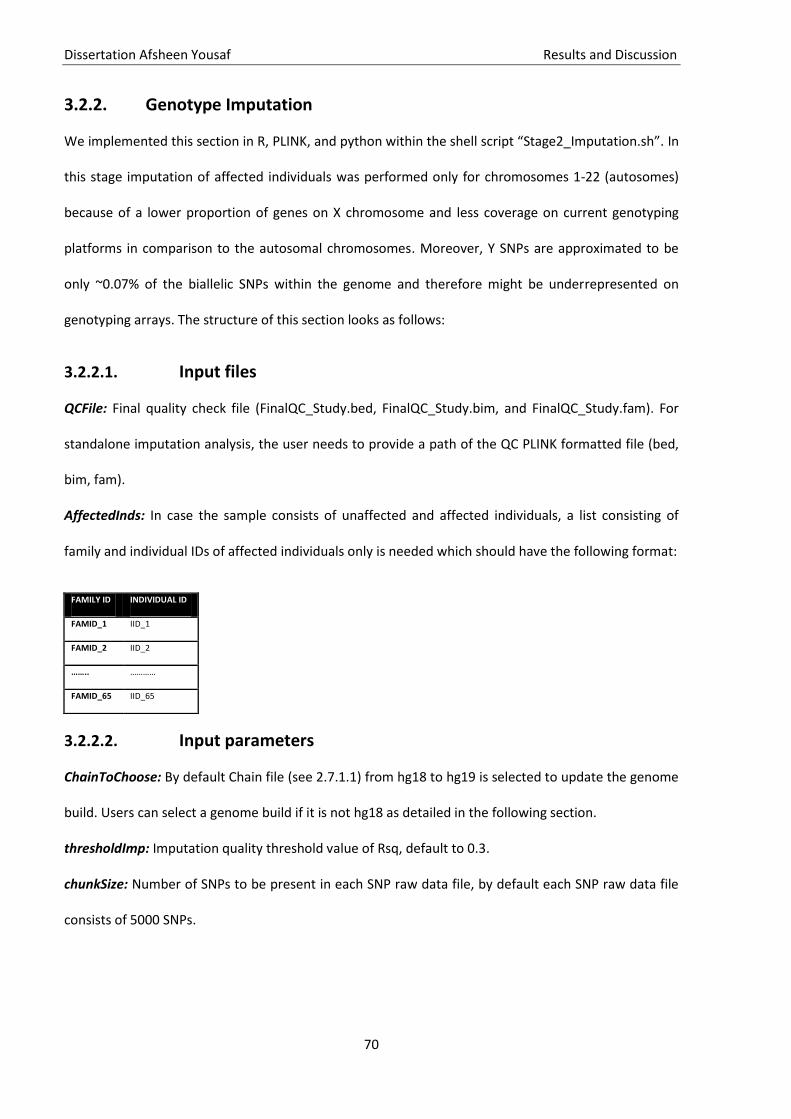
Dissertation Afsheen Yousaf Results and Discussion
70
3.2.2. Genotype Imputation
We implemented this section in R, PLINK, and python within the shell script “Stage2_Imputation.sh”. In
this stage imputation of affected individuals was performed only for chromosomes 1-22 (autosomes)
because of a lower proportion of genes on X chromosome and less coverage on current genotyping
platforms in comparison to the autosomal chromosomes. Moreover, Y SNPs are approximated to be
only ~0.07% of the biallelic SNPs within the genome and therefore might be underrepresented on
genotyping arrays. The structure of this section looks as follows:
3.2.2.1. Input files
QCFile: Final quality check file (FinalQC_Study.bed, FinalQC_Study.bim, and FinalQC_Study.fam). For
standalone imputation analysis, the user needs to provide a path of the QC PLINK formatted file (bed,
bim, fam).
AffectedInds: In case the sample consists of unaffected and affected individuals, a list consisting of
family and individual IDs of affected individuals only is needed which should have the following format:
3.2.2.2. Input parameters
ChainToChoose: By default Chain file (see 2.7.1.1) from hg18 to hg19 is selected to update the genome
build. Users can select a genome build if it is not hg18 as detailed in the following section.
thresholdImp: Imputation quality threshold value of Rsq, default to 0.3.
chunkSize: Number of SNPs to be present in each SNP raw data file, by default each SNP raw data file
consists of 5000 SNPs.
FAMILY ID INDIVIDUAL ID
FAMID_1 IID_1
FAMID_2 IID_2
…….. …………
FAMID_65 IID_65

Dissertation Afsheen Yousaf Results and Discussion
71
3.2.2.3. Reference files
The user needs to download the following reference files in “RefData” folder.
Hg19SNPs: Hg19 SNPs file containing SNPs rs ids (SNP name), starting and ending bp position,
chromosome number.
Since the 1000 genomes dataset is based on the hg19 genome build, the study dataset needs to be
updated to this genome build. All chain files are provided in the reference data, which a user can
download.
Chain files can be downloaded from the links provided on the GitHub
https://github.com/SheenYo/MAGNET and can be saved in the RefData folder.
MapFile: Genetic map for 1000 genome data Phase3 consisting of three columns containing the
physical position (bp), the recombination rate (cM/Mb) and the genetic position (cM). This file along
with reference files for SHAPEIT are required to be downloaded.
The folder will contain files in the following three formats:
ShapeitRefHaps: This file consists of SNPs and the haplotypes where each line corresponds to a single
SNP consisting information about the two alleles of a SNP by each haplotype of an individual about the
chromosome number, SNP id, SNP position, and the first and second allele.
ShapeitRefLegend: The file describes the SNPs, where the columns correspond to SNP id, SNP position,
first and second allele.
ShapeitRefSample: The file contains information about reference individuals, i.e. Individual ID,
population, group, and sex.
AnnotationFile: A complete instruction on downloading the annotation file is provided in the readme
file at https://github.com/SheenYo/MAGNET. These files contain annotation based on SNP 142
genome build (SNP locations and alleles information extracted from the single nucleotide
polymorphism database (dbSNP)) separated based on chromosomes, each file consists of chromosome
number, base pair position, SNP name, and column with chromosome:base pair.
Dissertation Afsheen Yousaf Results and Discussion
72
3.2.2.4. Output
Gwas.Chr (1-22)_Study.Imputed.Output.dose: Contains allele dosages (allele counts) for imputed and
genotyped SNPs.
Gwas.Chr(1-22)_Study.Imputed.Output.erate: Contains estimated error rate for every imputed and
genotype marker.
Gwas.Chr(1-22)_Study.Imputed.Output.info: Contains information on both genotyped and imputed
SNPs.
Gwas.Chr(1-22)_Study.Imputed.Output.m3vcf.gz: Output file in vcf (variant calling file) format.
Gwas.Chr(1-22)_Study.Imputed.Output.rec: Recombination file containing switch error rate
(Percentage of possible switches in haplotype orientation that is required to recover the correct phase
in an individual 201) per interval.
Gwas.Chr(1-22)_Study.Imputed.Output.hapDose.gz: Contains dosage for each haplotype separately.
Gwas.Chr(1-22)_Study.Imputed.Output.hapLabel.gz: Contains haplotype labels.
Merged_FinalQC_SNPs_Data (bed, bim, fam): PLINK formatted files consisting filtered (Rsq >0.3) and
biallelic SNPs.
Data_SNPfile (1-22): Raw files with minor alleles each consisting of 5000 imputed SNPs.
3.2.3. GWAS
This step is implemented in R, python, and bash. The analysis is provided within shell script
“Stage3_GWAS.sh”. This section uses the MAGMA tool to map the SNPs to their respective genes and
perform gene-based analysis (see 2.9). Depending on the number of SNPs in the study, chunks are
created with a default chunk size of 5000 each. However, the user is free to choose a chunk size in the
configuration file.
Dissertation Afsheen Yousaf Results and Discussion
73
3.2.3.1. Input files
Data_SNPfile.raw: Raw files consisting of 5000 SNPs each.
phenofile: The user needs to provide a reference file named “phenofile” consisting of family ID,
individual ID and value of phenotype of interest (such as IQ) in the data folder, e.g in the table below:
FAMILY ID INDIVIDUAL ID TRAIT
FAMID_1 IID_1 49
FAMID_2 IID_2 103
……….. ………… ………..
FAMID_65 IID_65 112
3.2.3.2. Input parameters
Pheno: Name of the phenotype to be analysed, required for the naming of results.
ColManhattan: Color to be used for Manhattan plot besides the grey color scheme used for every
alternate chromosome, default is black color.
Further, the user needs to specify five arguments required for MAGMA analysis and plotting
Manhattan plots that are as follows:
windowSize: The default window size to look for the genes around a SNP is 5kb upstream and
downstream of the gene.
Covars: Name of covariates included in the regression model, the names should correspond to those in
the phenotype file provided, e.g by default “Sex, Age” are the two covariates provided, these names
are same as in the phenotype file.
Fixed: Names of random covariates included in the regression model, please note that the names
should correspond to those in the phenotype file provided as explained above.
snpsOfInterest: Specific set of SNPs of interest which will be highlighted in the Manhattan plot, e.g.
"rs377398625","rs557375998","rs10736578”
MagmaN: Sample size (Number of individuals) for which MAGMA will be conducted.
MagmaPERMP: Permuted p-value for MAGMA analysis, by default set to 0.05

Dissertation Afsheen Yousaf Results and Discussion
74
3.2.3.3. Reference files
MagmaRef: 1000 genomes PLINK formatted reference file.
MagmaSNPloc: The file contains chromosome, SNP identifier, position in morgans or centimorgans
(unit to denote the distance between two loci on a chromosome) which is mostly dummy coded as “0”
of the reference 1000 genome dataset.
MagmaGeneloc: This file consists of location information about genes in NCBI37 (National Center for
Biotechnology Information genome build 37), i.e. Entrez gene id, chromosome id, start and stop
position, strand information, and gene.
3.2.3.4. Output
Results file: For each chunk, regression output will be saved in this file consisting of beta, se (standard
error), t, p-value, and adjusted p-value.
Summary file: For each chunk regression output summary will be saved in this file.
Magma Result file: File consisting of complete MAGMA gene lists will be provided in the
Magma_pheno.genes_tabseparated.txt file.
Pheno.SignificantGenes: List of significant genes resulting from MAGMA analysis below the default
threshold of the empirical p-value of 0.05.
3.2.4. Enrichment analysis
The enrichment analysis is implemented in R-3.5, packages include kegga, WGCNA, igraph, and
cerebroViz. The analysis is wrapped in shell script “Stage4_Enrichment.sh”.
3.2.4.1. Input files
Pheno.SignificantGenes: List of significant genes resulting from MAGMA analysis that are below the
default threshold of empirical p-value of 0.05.
Magma Result file: File consisting of complete MAGMA gene lists will be provided in the
Magma_pheno.genes_tabseparated.txt file.

Dissertation Afsheen Yousaf Results and Discussion
75
R Pre-requisites: Requires R-packages "org.Hs.eg.db, annotate, WGCNA, igraph and purrr". These will
be automatically downloaded upon script runtime.
Detailed commands for updating the packages are also provided at
https://github.com/SheenYo/MAGNET.
3.2.4.2. Input parameters
GOeliteSpecies: The pipeline is based for human data only, by default the option is set to “Hs” for
homo sapiens.
GOElitefolder: Name of the folder where GO elite inputs are stored.
Outputfolder: Name of output folder where results of the downstream analysis will be stored.
MAGNETHome: Name of the main directory where MAGNET is installed.
3.2.4.3. Reference files
Kang et al. 4 transcriptome data set is included as reference data for this stage. These files are provided
with the tool.
Kang Universe: All genes from Kang dataset.
Kang genes: All genes which are in Kang modules.
KangData: File consisting of Kang expression data.
3.2.4.4. Output
The output produces the following files:
All_MagmaGenes_Symbols.txt: All MAGMA Entrez genes mapped with their gene symbols.
All_genesMAGMA_Imputed_Kang.txt: All genes which are present in MAGMA and in Kang dataset.
phenoEnrichment_ouput.txt: Output of enrichment analysis.
phenoGO_ElitePlot.pdf : Plots of top ten GO-terms.
phenoKEGG.pdf: Plots of top ten KEGG pathways.
phenoEnriched_Modules.pdf: Gene network plots of enriched modules.
Heatmap_EnrichedModules.pdf: Heatmap of enriched modules.

Dissertation Afsheen Yousaf Results and Discussion
76
Cross sectional and sagittal Brain views: Eigen gene values of module genes in Kang dataset are also
presented with respect to brain-specific regions.
We ran the MAGNET tool on an IQ trait from the German cohort and recorded the computational time
required to process each stage of it. The results are summarized in Table 6. The computational
requirements for each section are different. The QC section requires the minimum computational
requirements and does not require a computational server. Moreover, a comparison with other state-
of-the-art tools is provided in Table 7.
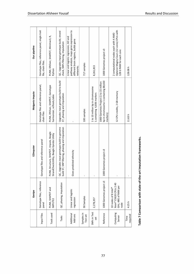
Dissertation Afsheen Yousaf Results and Discussion
77
G
en
ipe
EZIm
pu
ter
Mo
lgen
is-I
mp
ute
O
ur
pip
elin
e
Inp
ut
File
s G
eno
typ
e fi
les,
ref
eren
ce
pan
el
Gen
oty
pe
file
s an
d r
efe
ren
ce p
anel
G
eno
typ
e fi
les
and
ref
ere
nce
pan
el,
chai
n f
iles
Gen
oty
pe
file
s, r
efer
ence
pan
el, s
ingl
e tr
ait
file
, ch
ain
file
s.
Too
ls u
sed
P
LIN
K, S
HA
PEI
T an
d
IMP
UTE
2 P
LIN
K, S
tru
ctu
re, S
HA
PEI
T, Im
pu
te, B
eagl
e St
ran
dC
hec
kUti
lity,
Bea
gle
Gp
rob
s U
tilit
y P
LIN
K, l
iftO
ver,
SH
AP
EIT,
Gen
oty
pe
har
mo
niz
er, v
cfto
ols
,tab
ix
PLI
NK
; lif
tOve
r, S
HA
PEI
T, M
inim
ac3
, R,
Pyt
ho
n
Task
s Q
C, p
has
ing,
Imp
uta
tio
n
QC
, Up
grad
es in
pu
t ge
no
typ
e b
uild
to
gen
om
e b
uild
37
, SN
P f
ilter
ing,
ph
asin
g an
d im
pu
tati
on
U
pgr
ades
inp
ut
gen
oty
pe
bu
ild t
o b
uild
3
7, p
has
ing
and
imp
uta
tio
n
QC
, Up
grad
es in
pu
t ge
no
typ
e b
uild
, str
and
ch
eck,
SN
Ps
filt
eri
ng,
Imp
uta
tio
n
Ad
dit
ion
al
Ad
d-o
ns
Lin
ear
and
logi
stic
re
gres
sio
n
Giv
es p
red
icte
d e
thn
icit
y -
Lin
ear
and
logi
stic
reg
ress
ion
, GO
an
d
pat
hw
ay a
nal
ysis
, map
s ge
ne
exp
ress
ion
to
d
iffe
ren
t b
rain
reg
ion
s, b
uild
s ge
ne
net
wo
rks.
Sam
ple
s in
Te
st s
et
90
Sam
ple
s -
10
0 s
amp
les
71
7 s
amp
les
SNP
s in
Tes
t se
t 2
,27
8,3
57
- 1
to
10
mill
ion
bp
in c
hro
mo
som
e 1
.co
nta
inin
g 4
,83
6 m
arke
rs
8,2
61,
81
3
Ref
eren
ce
10
00
Gen
om
es p
roje
ct v
3
10
00
Gen
om
es p
roje
ct v
3
10
00
Gen
om
es P
roje
ct (
1 t
o 1
5 m
illio
n
bp
in c
hro
mo
som
e 1
co
nta
inin
g 8
8,6
50
m
arke
rs)
10
00
Gen
om
es p
roje
ct v
3
Co
mp
uti
ng
Serv
er
10
no
des
of
8 In
tel®
X
eon
® E
56
20
CP
Us
2.4
0
GH
z, 4
8G
of
RA
M p
er
no
de
- 1
2 C
PU
cre
dit
s, 2
GB
mem
ory
2
co
mp
uta
tio
nal
no
des
eac
h w
ith
4 A
MD
O
pte
ron
Mag
ny
Co
urs
(1
2 c
ore
s) C
PU
s w
ith
1
28
G R
AM
fo
r ea
ch c
ore
Tim
e re
qu
ired
4
:25
h
- 1
1:6
3 h
1
28
:08
h
Tab
le 7
Co
mp
aris
on
wit
h s
tate
-of-
the
-art
Imp
uta
tio
n f
ram
ew
ork
s.
Dissertation Afsheen Yousaf Results and Discussion
78
MAGNET-lite 3.3.
We also developed a GUI (Graphical User Interface) for the enrichment analysis. The interface is
developed in the R shiny package which builds interactive web apps using R. This interface was
developed by Miriam Hana Ulbrich in her internship project under my supervision. Shiny is an R
package that makes it easy to build interactive web apps straight from R.
Features
MAGNET-lite consists of the following features:
The user only needs to provide a gene list consisting of Entrez ids or gene symbols.
Pathway enrichment analysis is performed at the backend using GO-elite and R package kegga.
Bar plots are created for the top ten most significant GO-terms and KEGG pathways
Brain enrichment analysis is performed based on the user-provided gene lists.
Heatmaps of enriched modules and topmost connected gene networks are created.
All plots are downloadable in pdf format.
Magnet-lite can also be downloaded from https://github.com/SheenYo/MAGNET and then can be run
as a web GUI.
Discussion 3.4.
This section contains parts of the article “MApping the Genetics of neuropsychiatric traits to molecular
NETworks of the human brain” available on bioaRxiv (10.1101/336776).
MAGNET performance
We developed a pipeline that integrates genotype, phenotype, and brain transcriptome data within a
single framework. To illustrate the run time problem in data integration, we evaluated the run time for
the different computation steps and the overall time required starting from the application of quality
checks to the identification of associated genes for IQ trait in the German cohort, see Table 6. The
complete framework for the ASD German cohort took ~4 days (i.e. ~113 hours) to complete on a
computing server using 2 nodes with AMD Opteron Magny Cours with each 12 cores CPUs and with
Dissertation Afsheen Yousaf Results and Discussion
79
128 GB RAM per node. Quality checks were finished within 5 minutes for a total of 715,724 SNPs and
3,343 individuals (German cohort before QC). The computational time directly depends on the sample
size and number of genotyped SNPs and may vary with the preferences to include, exclude or modify
flagged samples and SNPs. Imputation based on the 622,344 variants was done for the 717 ASD
affected individuals only and took 48:22 hours increasing the number of SNPs to 8,261,813. For ~8
million SNPs, regression analysis took 37 hours. Overall, the gene-based association test took 19
minutes. Hence on an average MAGNET can save the time required to set up, configure, handle in
between data generated and running individual steps. All scripts are arranged as easy to use
command-line interface with the flexibility to perform individual stages separately. To run the analysis
no high-end programming skills are required but a basic understanding of Linux and shell scripting
might be helpful to run the scripts on a computational cluster.
Comparison with state-of-the-art tools
We also compared the features of MAGNET with other tools that perform QC, imputation and
regression analysis such as “Genipe” 142, Ezimputer 202, and Molgenis-impute 11. MAGNET provides an
edge over Genipe as it provides extensive visual plots for each QC step and provides an additional
pathway and brain enrichment analysis. Likewise MAGNET is beneficial for the users who do not want
to provide their genetic data on an online server to perform genetic analysis due to legal issues.
EZImputer besides performing QC and imputation also provides predicted ethnicity estimates. It
actually provides a modular set of scripts for building an imputation workflow but does not provide an
automated manner of performing it. Molgenis-impute is a well-established pipeline but only provides
imputation workflow at the moment.
MAGNET is oriented towards researchers with limited computational skills of computing clusters who
do not want to invest time in setting up workflows and data handling from different genetic analyses.
Instead, MAGNET provides an automated pipeline within one shell. However, the user has the
flexibility to run individual parts of the pipeline provided the input files are available in the correct
format.
Dissertation Afsheen Yousaf Results and Discussion
80
MAGNET availability and cluster usage
MAGNET is available freely at Github under https://github.com/SheenYo/MAGNET. with complete
scripts that can be adjusted to the needs of the respective user. A web interface for MAGNET stage 4
called MAGNET-lite is also available for the users who are only interested to know the specific
biological pathways behind their trait of interest and can also be downloaded from
https://github.com/SheenYo/MAGNET and can be run as GUI. In addition, it can look for enrichment of
the genes of interest with respect to 29 different modules associated with distinct spatio-temporal
expression patterns of the human brain 4. MAGNET-lite can be used as a normal GUI for which no
programming or Linux experience is required.
To boost the processing time of MAGNET, the scripts for stage 2 and 3 are written to directly run on
high-performance computing environments, i.e. SLURM and PBS. The user does not need to perform
any further parallelization steps, as genotype imputation and regression analysis are adapted to run in
an automated fashion on the cluster.
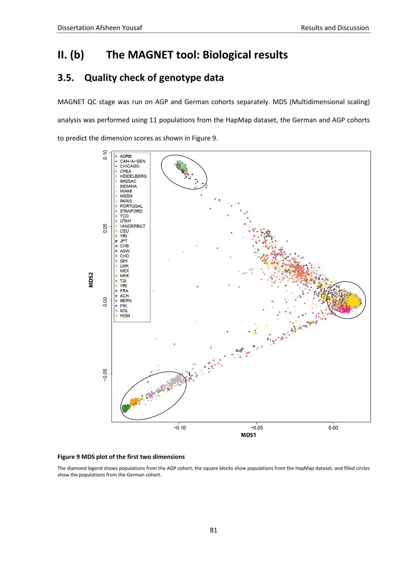
Dissertation Afsheen Yousaf Results and Discussion
81
II. (b) The MAGNET tool: Biological results
Quality check of genotype data 3.5.
MAGNET QC stage was run on AGP and German cohorts separately. MDS (Multidimensional scaling)
analysis was performed using 11 populations from the HapMap dataset, the German and AGP cohorts
to predict the dimension scores as shown in Figure 9.
Figure 9 MDS plot of the first two dimensions
The diamond legend shows populations from the AGP cohort, the square blocks show populations from the HapMap dataset, and filled circles show the populations from the German cohort.
Dissertation Afsheen Yousaf Results and Discussion
82
MDS plots showed the presence of three different clusters as the three main ethnicities, i.e. Asian,
African, and European. We selected the first four ethnicity components to be included in our analysis
for correcting population bias in the data. After QC, we only included affected individuals who had
complete genotype and phenotype data, i.e. data available for age and recruitment site information.
This resulted in 1,895 and 614 AGP and the German cohort affected individuals, respectively. A
detailed summary of data description is provided in Table 5. There was no difference in gender
distribution across cohorts (P= 0.373). The German cohort was older at diagnosis and showed a higher
IQ compared to the AGP sample. Moreover, no difference was observed between SI, PI, NVC, and RI
between the two cohorts. MAGNET provided a clean quality checked genotype file for each cohort. For
the next steps, MAGNET was run individually on each subdomain and for each cohort separately.
Imputation of missing genotype data 3.6.
The MAGNET imputation stage was run separately for each cohort and consisted only of affected
individuals. As we used the 1000 Genomes phase 3 data which is annotated based on GRCh37
coordinates we used liftOver to remove any genetic sample data which did not correspond to GRCh37
annotation. Additionally, SNPs which were only in the provided genotype data and not in the reference
data were also removed. SNP inconsistencies such as strand flip issues that cannot be resolved by
flipping were removed during the imputation. MAGNET provided multiple imputation output files as
detailed in 3.2.2.4, output was filtered based on the default imputation quality score of Rsq > 0.3
(removes > 70% of poorly-imputed SNPs at the cost of <0.5% well-imputed SNPs). The QC stage was
run again at the end of imputation to remove any SNPs that fall below the thresholds of QC. As our aim
was to identify the common variants observed in both cohorts, we manually selected SNPs that were
overlapping in both cohorts and extracted them from the genotype files of AGP and the German
cohort. This resulted in 6,900,500 SNPs overlapping in both cohorts with a MAF ≥ 2%. For efficient
processing, MAGNET divided the SNPs into 1,381 files, each file consisted of 5,000 SNPs in contrast to
Dissertation Afsheen Yousaf Results and Discussion
83
the last file which contained 500 SNPs. This division and assignment of SNPs are performed
automatically by MAGNET.
GWAS 3.7.
MAGNET stage 3, i.e. GWAS was first performed in the combined (AGP and German) cohort to account
for the power issues and to determine SNPs that might not reach genome-wide significance because of
the sample size of AGP and the German cohort. Later, MAGNET was also run on individual cohorts. The
sample size had a power of 1-beta > 80% to explain 6% of the variance (R2= 0.06) in the German cohort,
1.5% in the AGP cohort and 1.2% in the combined cohort with a genome-wide significance threshold of
alpha = 5e-8.
GWAS of the combined cohort resulted in eight genome-wide significant SNPs as shown in Table 8 and
Figure 10. Out of the eight SNPs, four were found for SI, i.e. rs2095092, P= 4.3 x 10-08 at chr.
(chromosome) 1p31.3 (closest gene PATJ: PALS1-Associated Tight Junction Protein); rs377634870, P=
4.8 x 10-08 at chr. 1p22.3 (no gene within 10kb); rs34459814, P= 2.5 x 10-08 at chr. 7q11.23 (closest gene
CLIP2: CAP-Gly Domain Containing Linker Protein 2); and rs34083004, P= 3.7 x 10-08 at chr. 7q11.23
(closest gene CLIP2). One SNP was found in PI, i.e. rs10115292, P= 1.8 x 10-08 at chr. 9p21.1 (no gene
within 10kb) and three in RB, i.e. rs13274146, P= 2.1x 10-08 at chr. 8p21.3 (no gene within 10kb);
rs7837513, P= 4.2x 10-09 at chr. 8p21.3 (no gene within 10kb); and rs7824610, P= 2.0 x 10-09 at chr.
8q21.11 (no gene within 10kb).
In the AGP cohort we identified nine genome-wide hits, two were identified for SI, i.e. rs377634870,
P= 4.8x10-08 at chr. 1p22.3 (no gene within 10kb), rs9333127, P= 4.75 x10-09 at chr. 10p13 (ITGA8:
Integrin Subunit Alpha 8), five were identified for PI, i.e. rs7777015, P= 4.75 x 10-09 at chr. 7q21.11 (no
gene within 10kb); rs6963792, P= 7.89x 10-09 at chr. 7q21.11 (no gene within 10kb); rs7783341,
P= 3.25 x 10-09 at chr. 7q21.11 (no gene within 10kb); rs9969152 , P= 1.65 x 10-09 at chr. 7q21.11 (no
gene within 10kb); and rs10115292, P= 4.73 x 10-08 at chr. 7q21.11 (no gene within 10kb). Two SNPs
were identified for RB, i.e. rs441459, P= 4.53 x 10-08 at chr. 11p15.4 (SLC22A18AS: Solute Carrier Family
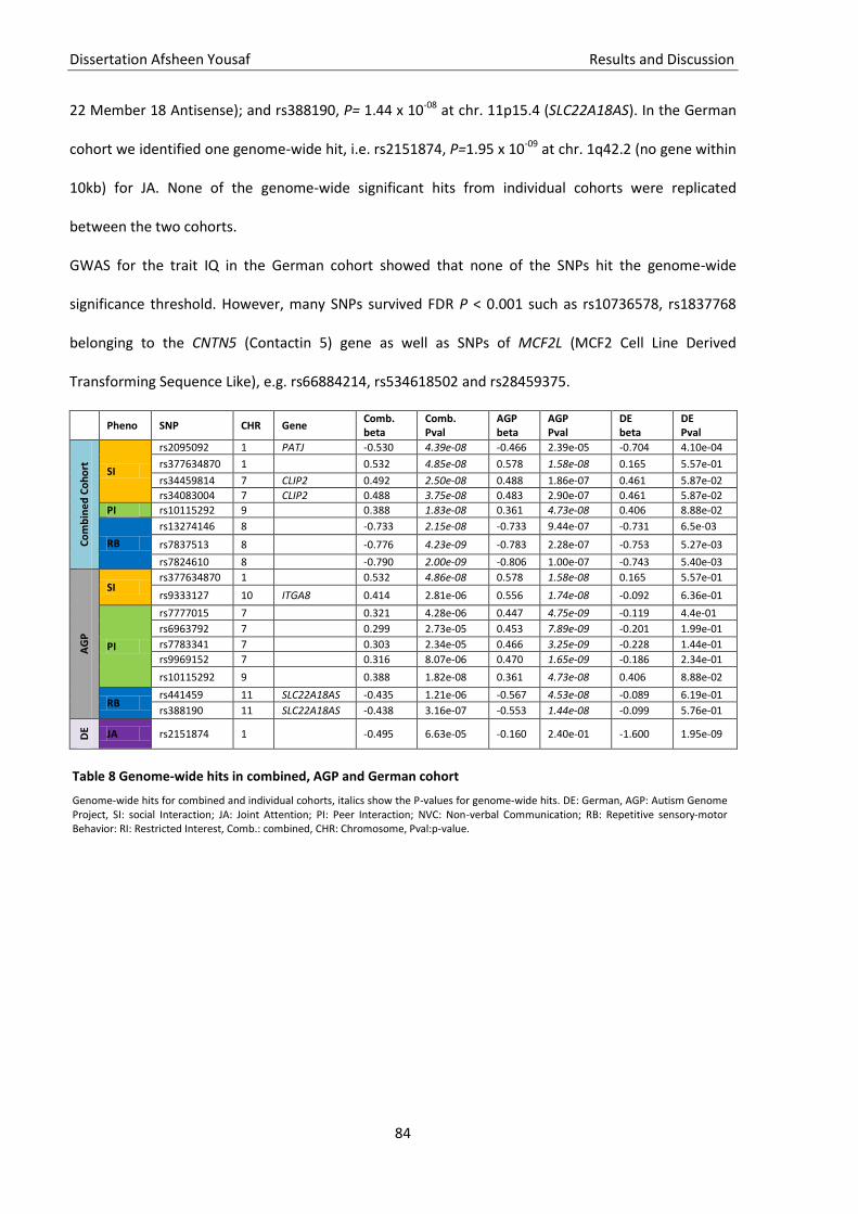
Dissertation Afsheen Yousaf Results and Discussion
84
22 Member 18 Antisense); and rs388190, P= 1.44 x 10-08 at chr. 11p15.4 (SLC22A18AS). In the German
cohort we identified one genome-wide hit, i.e. rs2151874, P=1.95 x 10-09 at chr. 1q42.2 (no gene within
10kb) for JA. None of the genome-wide significant hits from individual cohorts were replicated
between the two cohorts.
GWAS for the trait IQ in the German cohort showed that none of the SNPs hit the genome-wide
significance threshold. However, many SNPs survived FDR P < 0.001 such as rs10736578, rs1837768
belonging to the CNTN5 (Contactin 5) gene as well as SNPs of MCF2L (MCF2 Cell Line Derived
Transforming Sequence Like), e.g. rs66884214, rs534618502 and rs28459375.
Pheno SNP CHR Gene Comb. beta
Comb. Pval
AGP beta
AGP Pval
DE beta
DE Pval
Co
mb
ine
d C
oh
ort
SI
rs2095092 1 PATJ -0.530 4.39e-08 -0.466 2.39e-05 -0.704 4.10e-04
rs377634870 1 0.532 4.85e-08 0.578 1.58e-08 0.165 5.57e-01
rs34459814 7 CLIP2 0.492 2.50e-08 0.488 1.86e-07 0.461 5.87e-02
rs34083004 7 CLIP2 0.488 3.75e-08 0.483 2.90e-07 0.461 5.87e-02
PI rs10115292 9 0.388 1.83e-08 0.361 4.73e-08 0.406 8.88e-02
RB
rs13274146 8 -0.733 2.15e-08 -0.733 9.44e-07 -0.731 6.5e-03
rs7837513 8 -0.776 4.23e-09 -0.783 2.28e-07 -0.753 5.27e-03
rs7824610 8 -0.790 2.00e-09 -0.806 1.00e-07 -0.743 5.40e-03
AG
P
SI rs377634870 1 0.532 4.86e-08 0.578 1.58e-08 0.165 5.57e-01
rs9333127 10 ITGA8 0.414 2.81e-06 0.556 1.74e-08 -0.092 6.36e-01
PI
rs7777015 7 0.321 4.28e-06 0.447 4.75e-09 -0.119 4.4e-01
rs6963792 7 0.299 2.73e-05 0.453 7.89e-09 -0.201 1.99e-01
rs7783341 7 0.303 2.34e-05 0.466 3.25e-09 -0.228 1.44e-01
rs9969152 7 0.316 8.07e-06 0.470 1.65e-09 -0.186 2.34e-01
rs10115292 9 0.388 1.82e-08 0.361 4.73e-08 0.406 8.88e-02
RB rs441459 11 SLC22A18AS -0.435 1.21e-06 -0.567 4.53e-08 -0.089 6.19e-01
rs388190 11 SLC22A18AS -0.438 3.16e-07 -0.553 1.44e-08 -0.099 5.76e-01
DE JA rs2151874 1 -0.495 6.63e-05 -0.160 2.40e-01 -1.600 1.95e-09
Table 8 Genome-wide hits in combined, AGP and German cohort
Genome-wide hits for combined and individual cohorts, italics show the P-values for genome-wide hits. DE: German, AGP: Autism Genome Project, SI: social Interaction; JA: Joint Attention; PI: Peer Interaction; NVC: Non-verbal Communication; RB: Repetitive sensory-motor Behavior: RI: Restricted Interest, Comb.: combined, CHR: Chromosome, Pval:p-value.
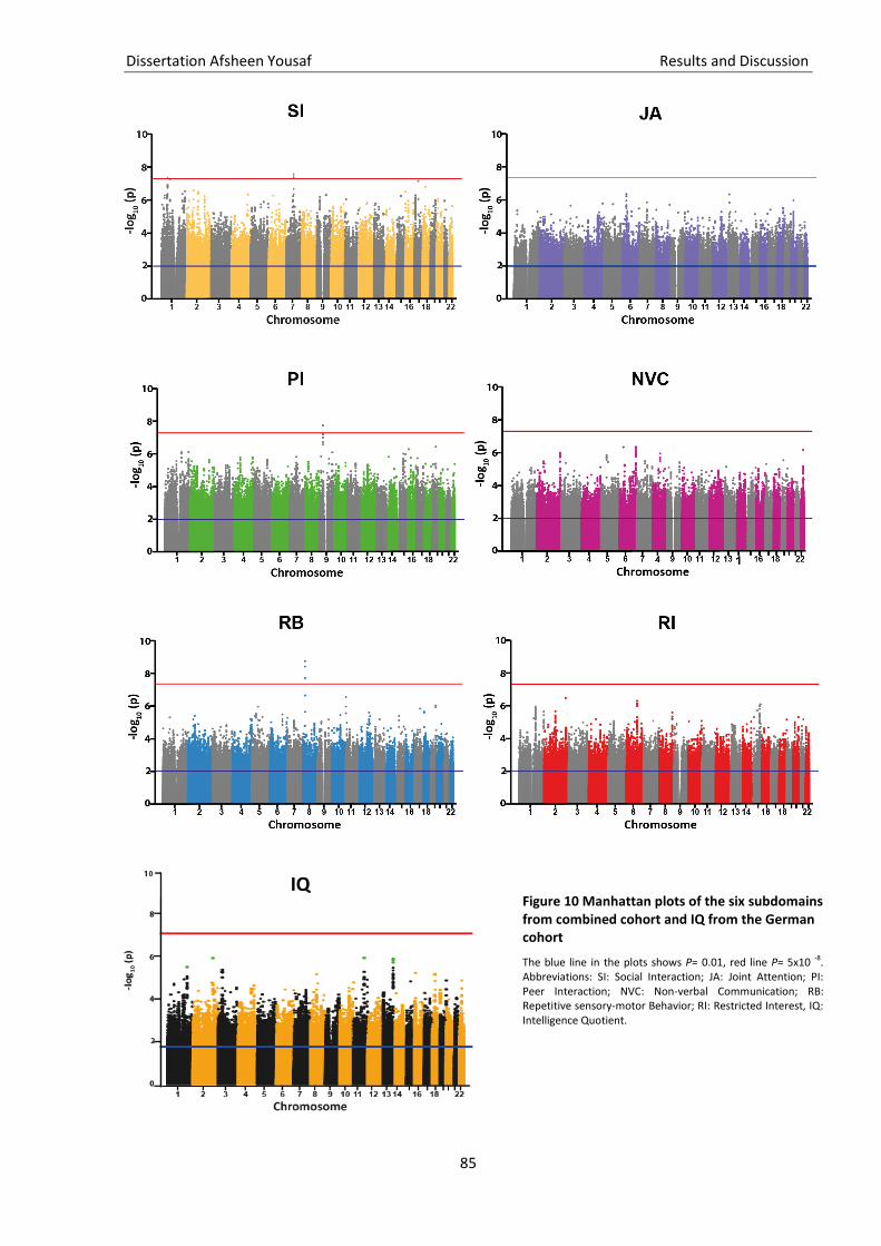
Dissertation Afsheen Yousaf Results and Discussion
85
IQ Figure 10 Manhattan plots of the six subdomains from combined cohort and IQ from the German cohort
The blue line in the plots shows P= 0.01, red line P= 5x10 -8. Abbreviations: SI: Social Interaction; JA: Joint Attention; PI: Peer Interaction; NVC: Non-verbal Communication; RB: Repetitive sensory-motor Behavior; RI: Restricted Interest, IQ: Intelligence Quotient.
Dissertation Afsheen Yousaf Results and Discussion
86
Gene and pathway analysis 3.8.
MAGNET stage 4, i.e. gene-based analysis using MAGMA was performed on the individual GWAS
outputs separately for each cohort. Since we wanted to identify the replicated genes in both cohorts,
SNPs were mapped to corresponding genes within a window of 5 kilobases (kb) up and downstream of
the respective hg19-annotated coding sequence. The significant genes (gene-wise empirical P< 0.05) to
be associated with the subscores that also overlapped in both cohorts are shown in Table 9. These
significant genes also contained some of the known ASD risk genes based on SFARI (Simons Foundation
Autism Research Initiative) database (https://gene.sfari.org/). We identified 52 genes associated with
SI which contained two ASD risk genes, i.e. GNAS (Guanine Nucleotide Binding Protein (G Protein)) and
PATJ (Protein Associated To Tight Junctions). For JA, we found 35 overlapping genes that also
contained the ASD risk gene DAGLA (Diacylglycerol Lipase Alpha). Similarly, in PI, 59 overlapping genes
were identified having four ASD risk genes, i.e. CECR2 (Cat Eye Syndrome Chromosome Region,
Candidate 2), MYO1E (Myosin IE), PGLYRP2 (Peptidoglycan Recognition Protein 2), and SCN5A (Sodium
Voltage-Gated Channel Alpha Subunit 5). For NVC, we identified 47 genes encompassing the ASD risk
genes ICA1 (Islet Cell Autoantigen 1), SCN8A (Sodium Voltage-Gated Channel Alpha Subunit 8) and
THRA (Thyroid Hormone Receptor Alpha). We identified 49 genes associated with RB including CMIP
(C-Maf Inducing Protein) and RNPS1 (RNA Binding Protein With Serine Rich Domain 1) which were
previously identified as ASD risk genes. The 59 genes implicated in RI also include ERBB4 (Erb-B2
Receptor Tyrosine Kinase 4) ASD risk gene.
For the trait IQ in the Geman cohort, MAGMA mapped ~ 8 million variants to 18,267 genes. Out of
these genes, 996 significant genes were identified with an empirical P< 0.05. The identified top three
most significant hits from MAGMA analysis are genes belonging to the S100 family, namely S100A3
(S100 calcium-binding protein A3), S100A4 (S100 calcium-binding protein A4), and S100A5 (S100
calcium-binding protein A5).
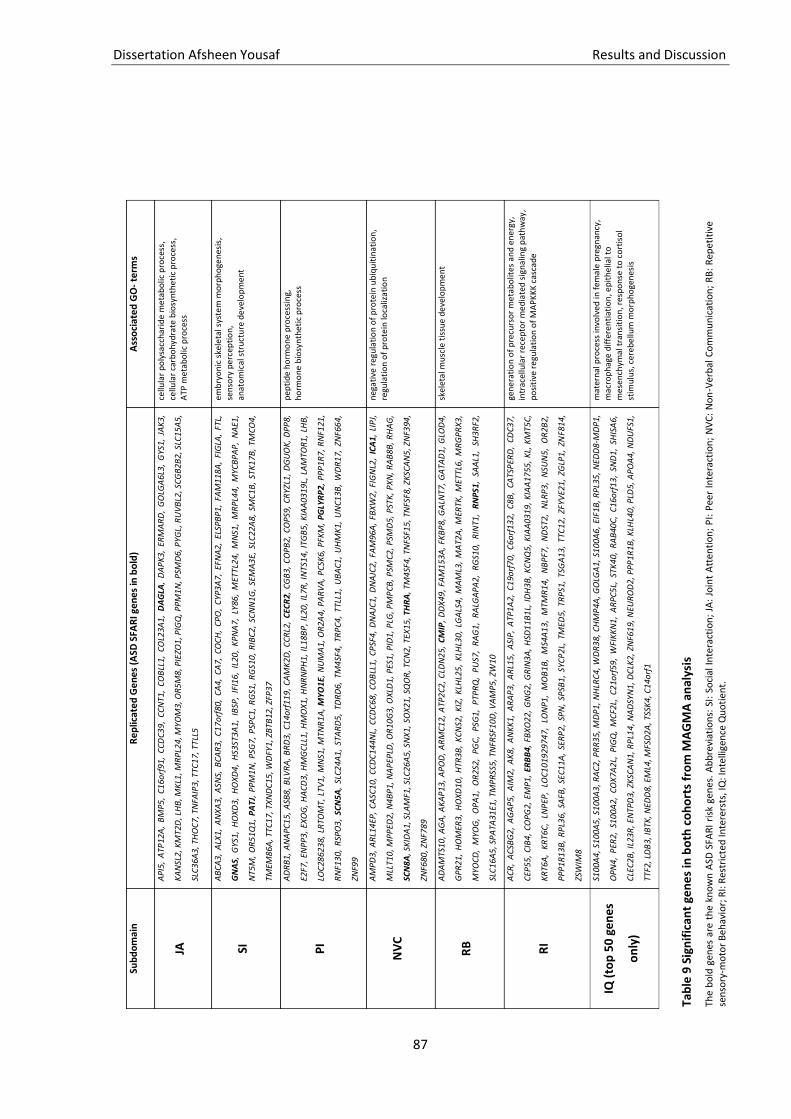
Dissertation Afsheen Yousaf Results and Discussion
87
Sub
do
mai
n
Re
plic
ate
d G
en
es
(ASD
SFA
RI g
en
es
in b
old
) A
sso
ciat
ed
GO
- te
rms
JA
AP
I5,
ATP
12A
, B
MP
5,
C1
6orf
91
, C
CD
C3
9,
CC
NT1
, C
OB
LL1,
CO
L23A
1,
DA
GLA
, D
AP
K3,
ER
MA
RD
, G
OLG
A6L
3, G
YS1,
JA
K3
,
KA
NSL
2, K
MT2
D, L
HB
, MK
L1, M
RP
L24,
MYO
M3,
OR
5M
8, P
IEZO
1, P
IGQ
, PP
M1
N, P
SMD
6, P
YGL,
RU
VB
L2, S
CG
B2B
2, S
LC1
5A
5,
SLC
36A
3, T
HO
C7,
TN
FAIP
3, T
TC1
7, T
TLL5
cellu
lar
po
lysa
cch
arid
e m
eta
bo
lic p
roce
ss,
cellu
lar
carb
oh
ydra
te b
iosy
nth
eti
c p
roce
ss,
ATP
me
tab
olic
pro
cess
SI
AB
CA
3, A
LX1,
AN
XA
3, A
SNS,
BC
AR
3,
C1
7o
rf80
, C
A4,
CA
7, C
OC
H,
CP
O,
CYP
3A7,
EFN
A2,
ELS
PB
P1
, FA
M11
8A,
FIG
LA,
FTL,
GN
AS,
GYS
1, H
OX
D3,
HO
XD
4,
HS3
ST3
A1
, IB
SP,
IFI1
6,
IL20
, K
PN
A7,
LY8
6,
MET
TL2
4, M
NS1
, M
RP
L44,
MYC
BP
AP
, N
AE1
,
NT5
M,
OR
51
Q1
, P
ATJ
, P
PM
1N
, P
SG7
, P
SPC
1,
RG
S1,
RG
S10
, R
IBC
2, S
CN
N1G
, SE
MA
3E,
SLC
22A
8, S
MC
1B,
STK
17B
, TM
CO
4,
TMEM
86A
, TTC
17,
TX
ND
C1
5, W
DFY
1, Z
BTB
12, Z
FP3
7
emb
ryo
nic
ske
leta
l sys
tem
mo
rph
oge
nes
is,
sen
sory
per
cep
tio
n,
anat
om
ical
str
uct
ure
de
velo
pm
en
t
PI
AD
RB
1, A
NA
PC
15
, A
SB8
, B
LVR
A,
BR
D3
, C
14
orf
11
9,
CA
MK
2D,
CC
RL2
, C
ECR
2,
CG
B3,
CO
PB
2, C
OP
S9,
CR
YZL1
, D
GU
OK
, D
PP
8,
E2F7
, EN
PP
3,
EXO
G,
HA
CD
3,
HM
GC
LL1,
HM
OX
1, H
NR
NP
H1
, IL
18B
P,
IL20
, IL
7R,
INTS
14,
ITG
B5
, K
IAA
031
9L,
LAM
TOR
1,
LHB
,
LOC
2862
38,
LR
TOM
T, L
TV1
, M
NS1
, M
TNR
1A
, M
YO
1E,
NU
MA
1, O
R2A
4, P
AR
VA
, P
CSK
6, P
FKM
, P
GLY
RP
2,
PP
P1R
7,
RN
F121
,
RN
F13
0, R
SPO
3,
SCN
5A
, SL
C2
4A
1,
STA
RD
5, T
DR
D6
, TM
4SF
4,
TRP
C4
, TT
LL1
, U
BA
C1
, U
HM
K1
, U
NC
13B
, W
DR
17,
ZN
F66
4,
ZNF9
9
pep
tid
e h
orm
on
e p
roce
ssin
g,
ho
rmo
ne
bio
syn
thet
ic p
roce
ss
NV
C
AM
PD
3, A
RL1
4EP
, C
ASC
10,
CC
DC
14
4N
L, C
CD
C6
8,
CO
BLL
1, C
PSF
4,
DN
AJC
1, D
NA
JC2
, FA
M96
A,
FBX
W2
, FI
GN
L2,
ICA
1,
LIP
J,
MLL
T10
, MP
PED
2,
N4
BP
1, N
AP
EPLD
, OR
10
G3
, OX
LD1,
PES
1, P
ID1
, PLG
, PM
PC
B,
PSM
C2
, PSM
D5,
PST
K,
PX
N, R
AB
8B,
RH
AG
,
SCN
8A
, SK
IDA
1, S
LAM
F1, S
LC26
A5
, SN
X1
, SO
X2
1, S
QO
R, T
CN
2, T
EX1
5, T
HR
A, T
M4
SF4,
TN
FSF1
5, T
NFS
F8, Z
KSC
AN
5, Z
NF3
94
,
ZNF6
80, Z
NF7
89
neg
ativ
e r
egu
lati
on
of
pro
tein
ub
iqu
itin
atio
n,
regu
lati
on
of
pro
tein
loca
liza
tio
n
RB
AD
AM
TS10
, A
GA
, A
KA
P1
3,
AP
OD
, A
RM
C1
2, A
TP2
C2
, C
LDN
25,
CM
IP,
DD
X49
, FA
M1
53A
, FK
BP
8, G
ALN
T7,
GA
TAD
1,
GLO
D4
,
GP
R2
1, H
OM
ER3,
HO
XD
10
, H
TR3
B,
KC
NS2
, K
IZ,
KLH
L25
, K
LHL3
0,
LGA
LS4
, M
AM
L3,
MA
T2A
, M
ERTK
, M
ETTL
6,
MR
GP
RX
3,
MYO
CD
, M
YOG
, O
PA
1,
OR
2S2,
PG
C,
PSG
1, P
TPR
Q,
PU
S7,
RA
G1
, R
ALG
AP
A2
, R
GS1
0, R
INT1
, R
NP
S1,
SAA
L1,
SH3
RF2
,
SLC
16A
5, S
PA
TA31
E1, T
MP
RSS
5, T
NFR
SF1
0D
, VA
MP
5, Z
W10
skel
etal
mu
scle
tis
sue
de
velo
pm
en
t
RI
AC
R,
AC
SBG
2,
AG
AP
5, A
IM2,
AK
8,
AN
KK
1,
AR
AP
3, A
RL1
5,
ASI
P,
ATP
1A2,
C1
9orf
70,
C6o
rf1
32,
C8B
, C
ATS
PER
D,
CD
C3
7,
CEP
55,
CIB
4,
CO
PG
2, E
MP
1,
ERB
B4
, FB
XO
22
, G
NG
2,
GR
IN3A
, H
SD1
1B1
L, I
DH
3B,
KC
NQ
5, K
IAA
0319
, K
IAA
1755
, K
L, K
MT5
C,
KR
T6A
, K
RT6
C,
LNP
EP,
LOC
10
192
97
47
, LO
NP
1,
MO
B1B
, M
S4A
13
, M
TMR
14,
N
BP
F7,
ND
ST2
, N
LRP
3,
NSU
N5
, O
R2
B2
,
PP
P1
R1
3B,
RP
L36,
SA
FB,
SEC
11A
, SE
RP
2, S
PN
, SP
SB1
, SY
CP
2L,
TM
ED5,
TR
PS1
, TS
GA
13,
TTC
12,
ZFYV
E21
, ZG
LP1
, ZN
F81
4,
ZSW
IM8
gen
era
tio
n o
f p
recu
rso
r m
eta
bo
lites
an
d e
ner
gy,
intr
acel
lula
r re
cep
tor
me
dia
ted
sig
nal
ing
pat
hw
ay,
po
siti
ve r
egu
lati
on
of
MA
PK
KK
cas
cad
e
IQ (
top
50
ge
ne
s
on
ly)
S100
A4
, S1
00A
5, S
100
A3
, RA
C2
, PR
R3
5, M
DP
1,
NH
LRC
4, W
DR
38,
CH
MP
4A, G
OLG
A1,
S1
00A
6,
EIF1
B, R
PL3
5,
NED
D8
-MD
P1
,
OP
N4
, P
ER2,
S1
00A
2,
CO
X7
A2
L, P
IGQ
, M
CF2
L, C
21o
rf59
, W
FIK
KN
1,
AR
PC
5L,
STK
40,
RA
B40
C,
C16
orf
13
, SN
D1
, SH
ISA
6,
CLE
C2
B, I
L23R
, EN
TPD
3, Z
KSC
AN
1, R
PL1
4,
NA
DSY
N1
, DC
LK2,
ZN
F61
9, N
EUR
OD
2, P
PP
1R1B
, K
LHL4
0, P
LD5,
AP
OA
4, N
DU
FS1
,
TTF2
, LD
B3,
IBTK
, NED
D8,
EM
L4, M
FSD
2A, T
SSK
4, C
14
orf
1
mat
ern
al p
roce
ss in
volv
ed in
fem
ale
pre
gnan
cy,
mac
rop
hag
e d
iffe
ren
tiat
ion
, ep
ith
elia
l to
m
esen
chym
al t
ran
siti
on
, res
po
nse
to
co
rtis
ol
stim
ulu
s, c
ereb
ellu
m m
orp
ho
gen
esis
Tab
le 9
Sig
nif
ican
t ge
ne
s in
bo
th c
oh
ort
s fr
om
MA
GM
A a
nal
ysis
The
bo
ld g
enes
are
th
e kn
ow
n A
SD S
FAR
I ri
sk g
enes
. A
bb
revi
atio
ns:
SI:
So
cial
In
tera
ctio
n;
JA:
Join
t A
tten
tio
n;
PI:
Pee
r In
tera
ctio
n;
NV
C:
No
n-V
erb
al C
om
mu
nic
atio
n;
RB
: R
epet
itiv
e
sen
sory
-mo
tor
Beh
avio
r; R
I: R
estr
icte
d In
tere
rsts
, IQ
: In
telli
gen
ce Q
uo
tien
t.
Dissertation Afsheen Yousaf Results and Discussion
88
GO-term analysis 3.9.
Overlapping MAGMA genes from each subdomain were selected manually for the subsequent analysis.
The overlapping gene list obtained for each subdomain was submitted to MAGNET stage 4. All
together, unique and significant GO-terms (permuted p-value < 0.05) in SI, JA, PI, NVC, RB, and RI were
9, 14, 22, 11, 3 and 12, respectively. IQ which was only analysed in the German cohort showed 190
significant pathways. The top significant GO-terms are shown in Figure 11. These are diverse processes
such as SI associated with the GO-term “sensory perception” among others. For JA the overlapping
genes were enriched for “carbohydrate metabolism”, “energy metabolism” and “chromatin
modification”. Similarly, in PI, enriched GO-terms included “hormone processing” and “plasma
membrane”. For NVC we identified GO-terms related to “protein catabolism”. RB was enriched for the
GO-terms “skeletal tissue muscle development” and “transmembrane receptor”. Enriched GO-terms
for RI were related to “postsynaptic signaling” and “intracellular mediated signaling pathways”. The
top GO-terms for IQ in the German data included GO-term analysis revealed processes such as
“cerebellar cortex neuron differentiation” and cerebellum morphogenesis”.
KEGG pathway analysis 3.10.
MAGNET provided the list of all enriched KEGG pathways, the number of genes in the KEGG pathway
and the number of genes associated with the input list and p-value for over-representation of the
KEGG term in the set. The KEGG pathways were limited due to the conservative approach applied for
selecting the set of significant genes. A few interesting pathways include “Starch and sucrose
metabolism” for JA, “Glucagon signaling pathway” for SI, “Metabolic pathways” for PI, “Sulfur
metabolism” for NVC, “FoxO signaling pathway” for RB and “cAMP signaling pathway” for RI. Whereas
for IQ from the German cohort, the enriched KEGG pathways include “VEGF signaling pathway”. The
most significant KEGG pathways for IQ included “Basal cell carcinoma” and “Melanogenesis”. These
pathways are shown in Figure 12.

Dissertation Afsheen Yousaf Results and Discussion
89
Brain enrichment analysis 3.11.
The final stage of MAGNET uses Kang et al. brain transcriptome data set to find enrichment of the
significantly overlapping genes from both cohorts for each subdomain in 29 different modules that are
co-regulated during the development of the human brain. Significantly overlapping genes from both
cohorts in each subdomain were then looked for enrichment in the Kang dataset. Enrichment was
found only for SI and NVC in Kang module 6 and module 27 respectively, showing a distinct pattern of
gene expression across time and brain regions. Module 6 shows a gene expression pattern that is
activated during toddlerhood and remains down-regulated between early and late childhood
specifically in the hippocampus. However, in the frontal cortex and striatum, the genes are upregulated
during childhood (Figure 13a). As per the information provided by Kang et al., module 6 is involved in
GO-terms related to “transport”. On the other hand, the gene expression pattern of module 27 genes
shows upregulation right after post-conception till middle childhood and then remains down-regulated
from late childhood onwards except in the hippocampus which is down-regulated during early to late
childhood (Figure 13b). Module 27 is related to GO-terms associated with “extracellular matrix” and
“cell-adhesion”.
Similarly, IQ trait in the German cohort showed to be enriched for modules 4 and 14. Module 4 is up-
regulated from early childhood to late adulthood in all brain regions other than the hippocampus,
while the gene expression pattern of module 14 shows up-regulation between early and late
childhood. Module 4 is involved in GO-terms related to “immune response”, and module 14 is
associated with “mitochondria”. Gene interaction networks of the enriched modules are also provided
to integrate the associated genes into the co-regulated modules. The provided graphs show the top 50
most connected genes and their transcriptomic correlation. Expression of the enriched modules and
gene networks of topmost connected genes are shown in Figure 13.
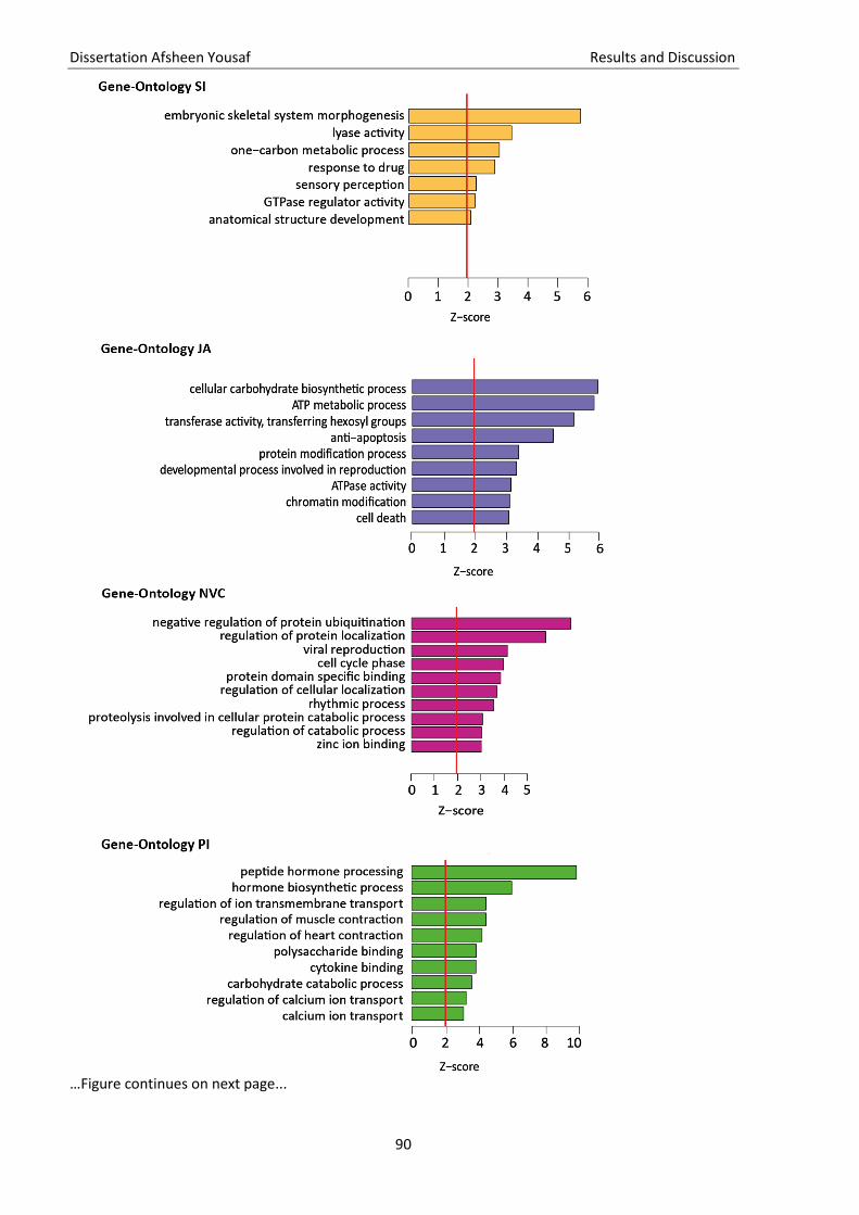
Dissertation Afsheen Yousaf Results and Discussion
90
…Figure continues on next page...
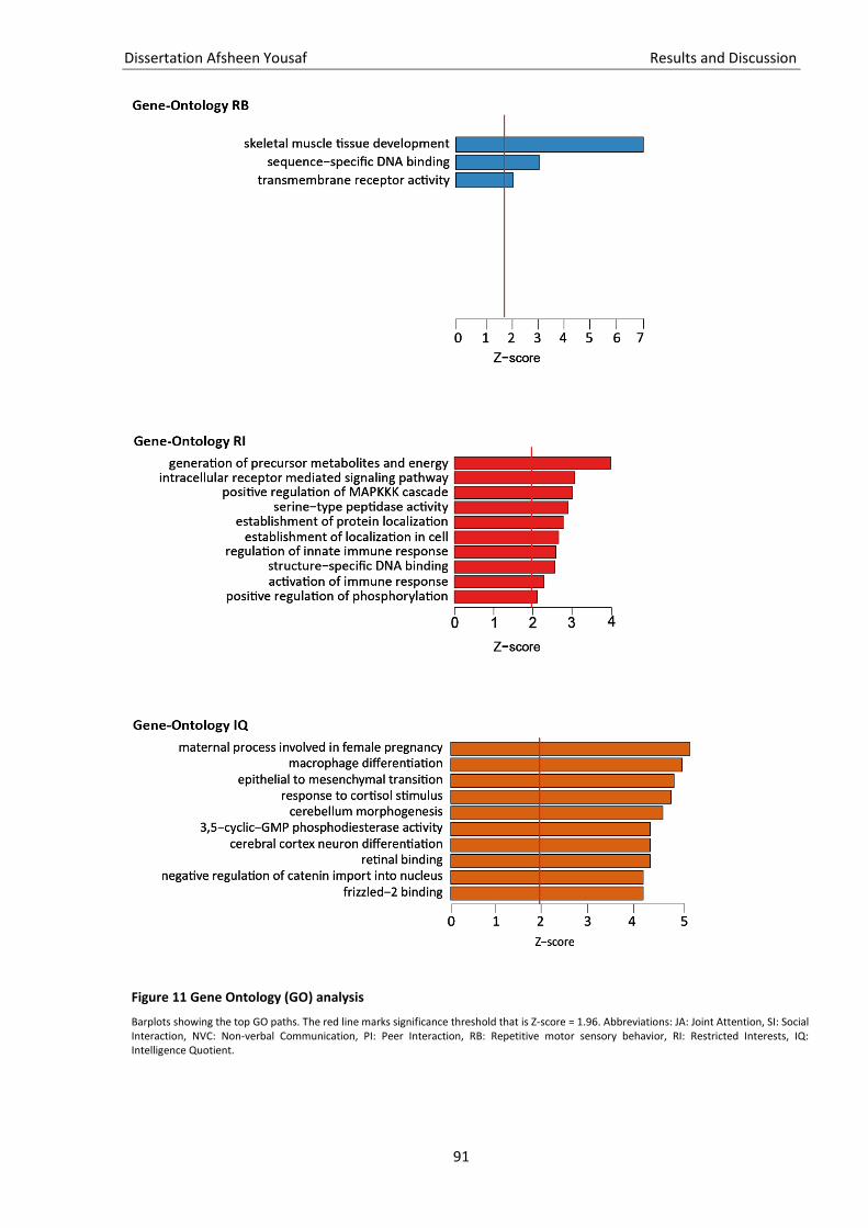
Dissertation Afsheen Yousaf Results and Discussion
91
Figure 11 Gene Ontology (GO) analysis
Barplots showing the top GO paths. The red line marks significance threshold that is Z-score = 1.96. Abbreviations: JA: Joint Attention, SI: Social Interaction, NVC: Non-verbal Communication, PI: Peer Interaction, RB: Repetitive motor sensory behavior, RI: Restricted Interests, IQ: Intelligence Quotient.
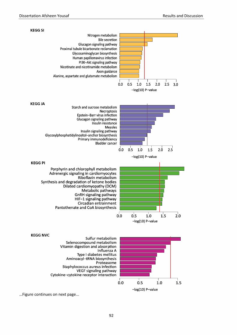
Dissertation Afsheen Yousaf Results and Discussion
92
…Figure continues on next page...
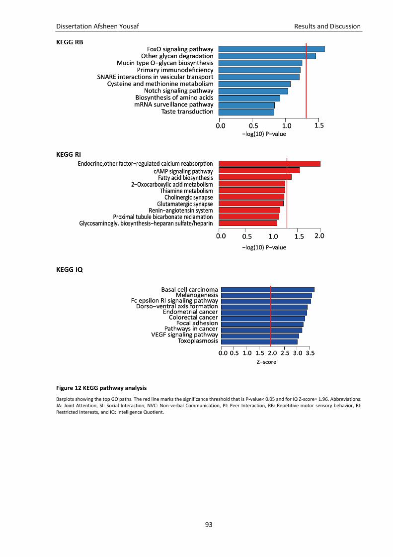
Dissertation Afsheen Yousaf Results and Discussion
93
Figure 12 KEGG pathway analysis
Barplots showing the top GO paths. The red line marks the significance threshold that is P-value< 0.05 and for IQ Z-score= 1.96. Abbreviations: JA: Joint Attention, SI: Social Interaction, NVC: Non-verbal Communication, PI: Peer Interaction, RB: Repetitive motor sensory behavior, RI: Restricted Interests, and IQ: Intelligence Quotient.
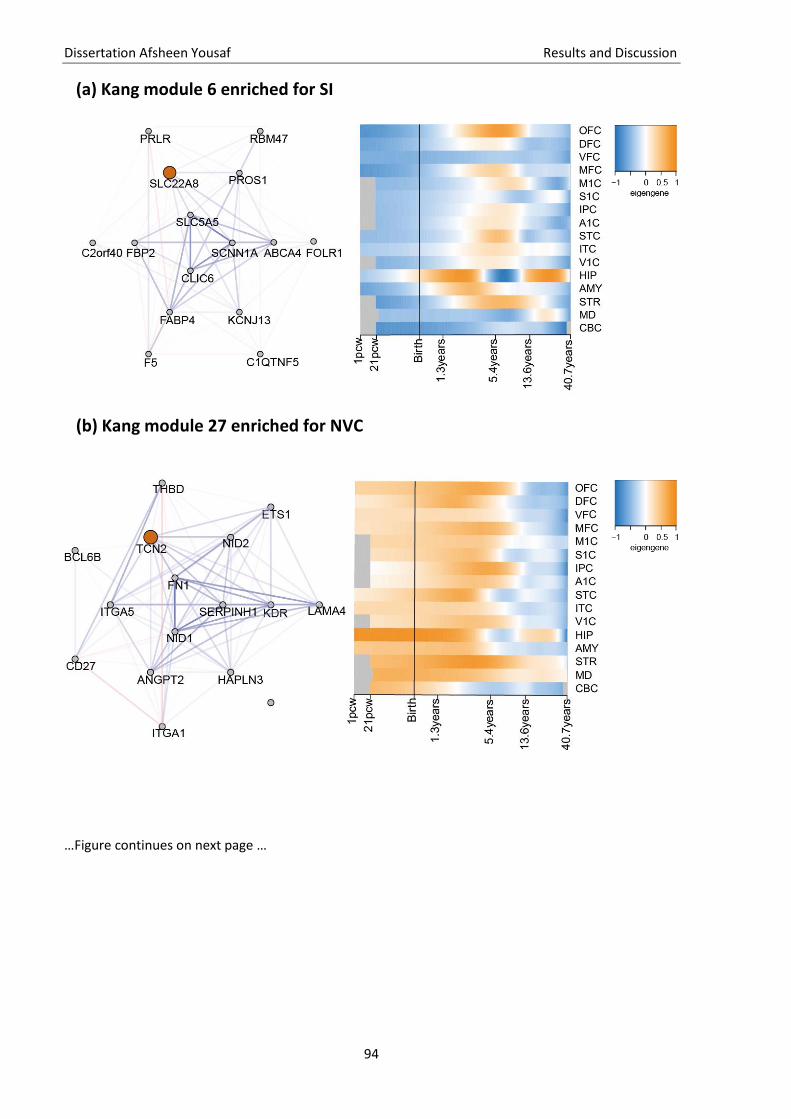
Dissertation Afsheen Yousaf Results and Discussion
94
…Figure continues on next page …
(a) Kang module 6 enriched for SI
(b) Kang module 27 enriched for NVC
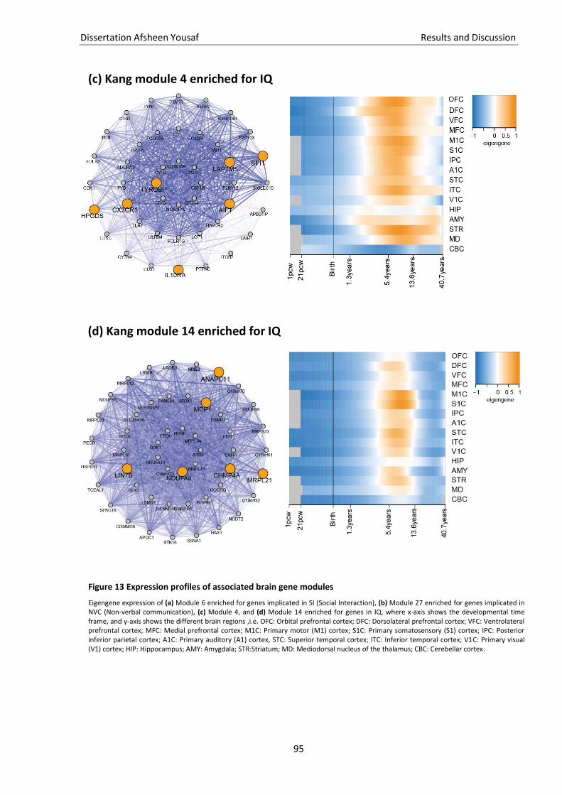
Dissertation Afsheen Yousaf Results and Discussion
95
Figure 13 Expression profiles of associated brain gene modules
Eigengene expression of (a) Module 6 enriched for genes implicated in SI (Social Interaction), (b) Module 27 enriched for genes implicated in NVC (Non-verbal communication), (c) Module 4, and (d) Module 14 enriched for genes in IQ, where x-axis shows the developmental time frame, and y-axis shows the different brain regions ,i.e. OFC: Orbital prefrontal cortex; DFC: Dorsolateral prefrontal cortex; VFC: Ventrolateral prefrontal cortex; MFC: Medial prefrontal cortex; M1C: Primary motor (M1) cortex; S1C: Primary somatosensory (S1) cortex; IPC: Posterior inferior parietal cortex; A1C: Primary auditory (A1) cortex, STC: Superior temporal cortex; ITC: Inferior temporal cortex; V1C: Primary visual (V1) cortex; HIP: Hippocampus; AMY: Amygdala; STR:Striatum; MD: Mediodorsal nucleus of the thalamus; CBC: Cerebellar cortex.
(c) Kang module 4 enriched for IQ
(d) Kang module 14 enriched for IQ
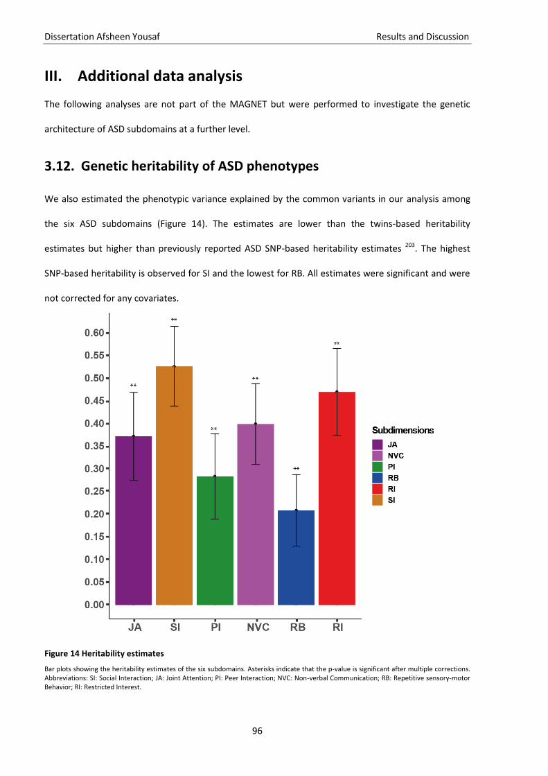
Dissertation Afsheen Yousaf Results and Discussion
96
III. Additional data analysis
The following analyses are not part of the MAGNET but were performed to investigate the genetic
architecture of ASD subdomains at a further level.
Genetic heritability of ASD phenotypes 3.12.
We also estimated the phenotypic variance explained by the common variants in our analysis among
the six ASD subdomains (Figure 14). The estimates are lower than the twins-based heritability
estimates but higher than previously reported ASD SNP-based heritability estimates 203. The highest
SNP-based heritability is observed for SI and the lowest for RB. All estimates were significant and were
not corrected for any covariates.
Figure 14 Heritability estimates
Bar plots showing the heritability estimates of the six subdomains. Asterisks indicate that the p-value is significant after multiple corrections. Abbreviations: SI: Social Interaction; JA: Joint Attention; PI: Peer Interaction; NVC: Non-verbal Communication; RB: Repetitive sensory-motor Behavior; RI: Restricted Interest.

Dissertation Afsheen Yousaf Results and Discussion
97
Correlation among ASD phenotypes 3.13.
We observed the phenotypic and genetic correlation among ASD subdomains. Phenotypically, the six
ASD subdomains appear to be significantly independent of each other. However, the domain A
subdomains of ASD, i.e. JA, SI, PI, and NVC are relatively closely clustered than the domain B
subdomains, i.e. RB and RI. At the genetic level, we observe that SI pairs with NVC, PI with JA, and
altogether, all these subdomains are also correlated with the exception of RB. The correlation of RB
was weak with all other subdomains although none of the correlations was significant (Figure 15b).
Figure 15 Heatmaps illustrating the (a) phenotypic and (b) genetic correlation among ASD subdomains
The color of squares represents the intensity of correlations depicted with a color range of yellow to blue showing a range of lowest to highest correlation respectively. Asterisks *** indicate p-values < 0.001. Abbreviations: JA: Joint Attention; PI: Peer Interaction; NVC: Non-verbal Communication; RB: Repetitive sensory-motor Behavior; RI: Restricted Interest.
PRS for ASD phenotypes 3.14.
The PRS for ASD explained a significant (all P< 2x10-05) proportion of the genetic variance of all
subdomains. Here, we report the best fit model for each of the subdomains. For SI the best fit
explained 3.3% of variance (R²), 2.3% in JA and in PI. For NVC and the domain B related subdomain RB,
a much lower R2 was observed, i.e. an R²= 0.7% and R²= 1.2%, respectively. In comparison, the other
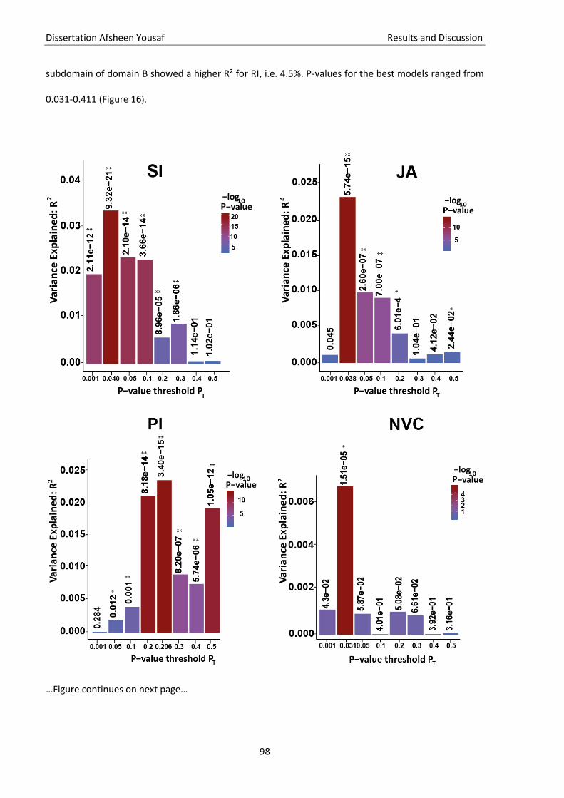
Dissertation Afsheen Yousaf Results and Discussion
98
subdomain of domain B showed a higher R² for RI, i.e. 4.5%. P-values for the best models ranged from
0.031-0.411 (Figure 16).
…Figure continues on next page…
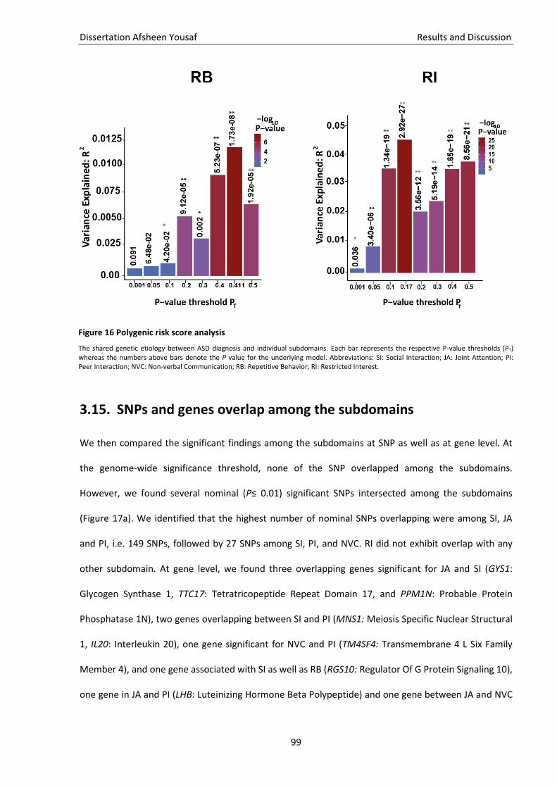
Dissertation Afsheen Yousaf Results and Discussion
99
SNPs and genes overlap among the subdomains 3.15.
We then compared the significant findings among the subdomains at SNP as well as at gene level. At
the genome-wide significance threshold, none of the SNP overlapped among the subdomains.
However, we found several nominal (P≤ 0.01) significant SNPs intersected among the subdomains
(Figure 17a). We identified that the highest number of nominal SNPs overlapping were among SI, JA
and PI, i.e. 149 SNPs, followed by 27 SNPs among SI, PI, and NVC. RI did not exhibit overlap with any
other subdomain. At gene level, we found three overlapping genes significant for JA and SI (GYS1:
Glycogen Synthase 1, TTC17: Tetratricopeptide Repeat Domain 17, and PPM1N: Probable Protein
Phosphatase 1N), two genes overlapping between SI and PI (MNS1: Meiosis Specific Nuclear Structural
1, IL20: Interleukin 20), one gene significant for NVC and PI (TM4SF4: Transmembrane 4 L Six Family
Member 4), and one gene associated with SI as well as RB (RGS10: Regulator Of G Protein Signaling 10),
one gene in JA and PI (LHB: Luteinizing Hormone Beta Polypeptide) and one gene between JA and NVC
Figure 16 Polygenic risk score analysis
The shared genetic etiology between ASD diagnosis and individual subdomains. Each bar represents the respective P-value thresholds (PT) whereas the numbers above bars denote the P value for the underlying model. Abbreviations: SI: Social Interaction; JA: Joint Attention; PI: Peer Interaction; NVC: Non-verbal Communication; RB: Repetitive Behavior; RI: Restricted Interest.
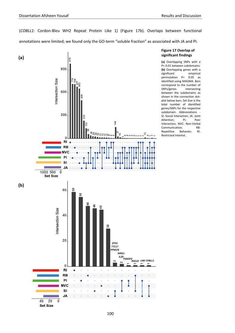
Dissertation Afsheen Yousaf Results and Discussion
100
(COBLL1: Cordon-Bleu WH2 Repeat Protein Like 1) (Figure 17b). Overlaps between functional
annotations were limited; we found only the GO-term “soluble fraction” as associated with JA and PI.
Figure 17 Overlap of significant findings
(a) Overlapping SNPs with a P< 0.01 between subdomains. (b) Overlapping genes with a significant empirical permutation P< 0.05 as identified using MAGMA. Bars correspond to the number of SNPs/genes intersecting between the subdomains as shown in the connection dot-plot below bars. Set Size is the total number of identified genes/SNPs for the respective subdomain. Abbreviations - SI: Social Interaction; JA: Joint Attention; PI: Peer Interaction; NVC: Non-Verbal Communication; RB: Repetitive Behavior; RI: Restricted Interest.
Dissertation Afsheen Yousaf Results and Discussion
101
Discussion 3.16.
This section contains parts of the article “Quantitative genome-wide association study of six
phenotypic subdomains identifies novel genome-wide significant variants in Autism Spectrum
Disorder” which has been submitted and is currently in the review process in the Journal of Translation
Psychiatry. The biological question behind this study was to characterize the underlying genetic
etiology and functional overlap behind ASD diagnostic domains and the respective subdomains.
Moreover, clinical studies have also shown that the phenotypic heterogeneity can be studied as
predictors of outcome in clinical trials 204. However, only a few studies have looked at its association
with the genetic underpinnings.
ADI-R defined ASD subdomains replicated previous structure
The two diagnostic domains of ASD defined by DSM-5 have been suggested as two separable domains,
i.e. social and repetitive behaviors identified by using factor analysis and principal component
analysis205. To date, information regarding the genetic etiology of these two domains remains limited
and the individual findings are not replicated in other cohorts. The possible reasons can be the small
genetic effect sizes and limited sample sizes.
Previously, it has been shown that defining separate ASD traits into more homogenous groups can
reduce the genetic heterogeneity 206. These subgroups might lead to direct expressions of gene effects
and also contribute in improving the effect sizes and thus the statistical power. Moreover, it can assist
in identifying susceptibility genes for ASD subgroups. In this study, we also identified a six-factor
structure that has been previously reported by Liu et al.84, as well as a similar structure was identified
from 98 ADI-R items 207. This six-factor structure was also confirmed in the independent German cohort
in this study. Thus, we postulate that the classification of ADI-R diagnostic domains into these
subdomains plays an important role and can serve as possible predictors in accessing the underlying
etiology.
Dissertation Afsheen Yousaf Results and Discussion
102
Association of common variants behind specific ASD subdomains in the combined,
AGP and, German cohort
GWAS analysis using MAGNET identified several genome-wide significant common variants and
respective novel candidate genes across the study. As GWAS was performed on the combined cohort
for power issues, we later followed a conservative approach to consider only the genes which
significantly replicated in both cohorts to be considered for the downstream analysis. We first discuss
the findings from the combined cohort and the significant genes replicated from gene analysis in both
cohorts.
Combined cohort (AGP and DE)
We identified four genome-wide common variants for SI. One mapped to an ASD-related gene PATJ
(Protein Associated To Tight Junctions), which codes for a scaffolding protein CIPP and regulates the
surface expression and/or function of ASIC3 (Acid-sensing ion channel 3) in sensory neurons 208.
A study found three case-specific loss-of-function variants (variants that disrupt the function of the
resulting proteins) in association with PATJ 209. Two other genome-wide hits map to CLIP2 (Cytoplasmic
Linker Protein 2) gene. This gene is located at chromosomal position 7q11.23 and duplication carriers
of this region show a high rate of ASD 210.
Though no genome-wide hit was identified for JA, the GWAS analysis for JA identified one of the top
three significant SNP peaks, consisting of rs10254837, rs4075496, and rs56263157 at 7q11.22 which
maps to the gene AUTS2. Genomic rearrangements of this gene are associated with ASD and
intellectual disability (ID) 211. In a study by Gao et al., Auts2-KO (knockout) mice showed impairments in
sensorimotor, cognition and communication behavior 212.
For PI we identified only one genome-wide significant SNP, i.e. rs10115292 mapped to an intergenic
region at chromosomal position 9p21.1, which is known for ASD-associated CNVs 28.
Though no genome-wide significant hit was identified for NVC, SNPs at a suggestive significance
P< 5x10⁻⁷ map to chromosomal position 6q26, a region linked to ASD 111. Moreover, this region has
Dissertation Afsheen Yousaf Results and Discussion
103
been associated with intellectual disability, delayed language development and dyspraxia in a case with
an 8Mb microdeletion of the 6q26-q27 locus 213.
For RB we identified three genome-wide SNPs which mapped to 8p21.3. This region has been
previously associated with restricted and repetitive behaviors in ASD 173. Duplications of this region
have been associated with ASD 214. Among the other top three SNP peaks, 19q13.33 was also identified
in RB. This region has also been shown previously to be associated with repetitive sensory-motor
behavior 84.
No genome-wide significant hit was observed for RI, however, the top significant SNP hits for RI were
also observed in migraine, sensorineural deafness, cognition, and ASD such as NLRP3 (NLR Family Pyrin
Domain Containing 3) 215, GNG2 (G Protein Subunit Gamma 2) 216 and NSUN5 (NOP2/Sun RNA
Methyltransferase 5) 217. The top peak at 15q25.3 is spanning the neurotrophic receptor tyrosine
kinase 3 gene NTRK3 (Neurotrophic Receptor Tyrosine Kinase 3), a gene previously associated with
both ASD and Asperger syndrome 218 as well as obsessive-compulsive disorder 219.
Individual cohorts
In the individual AGP cohort, we identified nine genome-wide hits. Two hits were identified in SI, i.e.
rs377634870 at chr1:84731827 (no nearest gene at 10kb) and rs9333127 at chr10:15658963 (ITGA8:
Integrin Subunit Alpha 8). ITGA8 is involved in sensory and motor neurons and the regulation of neurite
outgrowth. A missense mutation in this gene has been associated with schizophrenia 220. However, it
has not been investigated with respect to ASD. Similarly, five genome-wide hits were reported for PI
including rs7777015, rs6963792, rs7783341, rs9969152 at chr.7 (no nearest genes within 5kb). All
these SNPs are present at 7q21.11, a region known to be involved in ASD 111. Besides these SNPs,
rs10115292 at chromosome 9 (no nearest gene within 5kb) which is significant in the merged cohort, is
also genome-wide, significant in the AGP cohort. Genome-wide, significant SNPs have also been found
for RB, i.e. rs441459 and rs388190 at 11p15.4 mapping to the gene SLC22A18AS (Solute Carrier Family
22 Member 18 Antisense). This gene was found to be upregulated in a group of ASD individuals 221.
Dissertation Afsheen Yousaf Results and Discussion
104
We also identified two genome-wide significant hits in the German cohort. One in NVC, i.e. rs75158512
at chromosomal position 10p14, a region associated with ASD 222. Similarly, one SNP was identified for
JA, i.e. rs2151874 at 1q42.2. Previously, an inherited 2.07 Mb microduplication was found at this locus
in two brothers with ASD and mental retardation 223.
The separate GWAS on IQ trait from the German cohort identified gene variants of CNTN5
(rs10736578, rs1837768) and MCF2L (rs66884214, rs534618502, rs28459375), which have not been
identified before in the context of IQ directly. The SNPs of these newly IQ-associated genes were
among the top 10 SNPs with a P< 5x10⁻⁷ and an FDR-corrected P≤ 0.001. CNTN5 mediates cell surface
interactions during nervous system development and plays a role in axon connections 224. MCF2L
encodes Rho guanine nucleotide exchange factor (GEF) and is expressed in the human brain 225.
The results of GWAS analysis in combined and individual analysis strengthened the plausibility of our
findings as we not only identified novel variants and genes but also genes that were known to be
associated with ASD previously. Moreover, we deduce that the disassociation of ASD phenotypic
domains into specific subdomains led to an increase in statistical power as also previously proposed 206
and identification of genome-wide significant variants. Thus, this also validates the functioning of
MAGNET in relation to identification of trait-associated common variants and their respective genes.
Identification of overlapping genes in ASD cohorts subdomains
As mentioned earlier, we followed a conservative approach for selecting the genes for downstream
analysis to minimize the chance of false-positive findings. For this purpose, we only selected the genes
from gene analysis which had a significant empirical P< 0.05 in AGP and the German cohort
subdomains.
Based on MAGMA gene analysis, we identified 52 overlapping genes in SI, which include the genome-
wide significant SNP mapped gene PATJ as well as the gene FTL (Ferritin Light Chain), which is involved
in Neurodegeneration with Brain Iron Accumulation (NBIA) disorders 226 that are clinically characterized
by a progressive movement disorder with symptoms varying significantly in terms of range and

Dissertation Afsheen Yousaf Results and Discussion
105
severity, such as cognitive deficits, personality changes with impulsivity and violent outbursts,
depression, emotional lability, and obsessive-compulsive disorder 227
For JA, 35 overlapping genes showed significant association. Among the most significantly associated
genes we identified a neural stem cell-derived dendrite regulator protein-coding gene DAGLA
(Diacylglycerol Lipase Alpha) implicated in seizures and neurodevelopmental disorders including ASD
228, and the COBLL1 (Cordon-Bleu WH2 Repeat Protein Like 1) gene involved in epilepsy 229 and
language impairment 230.
In the gene set analysis for PI, 59 overlapping genes were identified as significantly associated. Among
these genes, we found a sodium voltage-gated ion channel gene SCN5A, which was found to be
enriched in an ASD-associated protein interaction module 231. Other ASD-associated, significant genes
include CECR2 (cat eye syndrome chromosome region candidate 2), a 7.2kb exonic loss of which was
found in an ASD female 228. Another interesting hit in the list is ENPP3 (Ectonucleotide
Pyrophosphatase), variants of this gene (ENPP4, ENPP5) have been associated with seven brain regions
in ASD, i.e. angular gyrus, anterior caudate, cingulate gyrus, dorsolateral prefrontal cortex,
hippocampus middle, inferior temporal lobe, and substantia nigra 232.
NVC showed 47 replicated genes in both cohorts. The gene SLC26A5 (Solute Carrier Family 26 Member
5) at 11p15.4 was among the top hits from the gene-based analysis. Mutations in this gene are
potential candidates for causing neurosensory deafness233. This region is also linked with the
development of speech83. Another important gene in the list is RGS10 (Regulator Of G Protein Signaling
10) which is known to be implicated in neurodegenerative diseases 234.
Top significant genes for RI were associated with migraine, sensorineural deafness, cognition, Williams-
Beuren syndrome and ASD such as NLPR3 215, GNG2 216and NSUN5 217.
The top three most significant hits from IQ gene analysis were the genes S100A3, S100A4, and S100A5.
Gene products of S100A5 are known to be expressed in the cerebral cortex and hippocampus, which
are important brain regions in ASD 235.
Dissertation Afsheen Yousaf Results and Discussion
106
Although we selected a conservative approach for selecting the gene list, we found that several genes
mapped from GWAS hits of the combined cohort were found at the gene level. This validates the
findings of our study and provides grounds for focusing on these genes further with respect to these
subdomains of ASD phenotypes.
Enrichment of distinctive pathways in ASD subdomains
To further identify the biological function of the enriched genes for each subdomain, we used MAGNET
to perform GO-term and pathway enrichment analysis. The analysis identified “sensory perception” as
one of the most significant pathways for SI. Atypicalities in sensory processing were found in families
which had higher genetic liability for ASD 236. For JA we identified that the topmost significant GO-term
“chromatin modification” is enriched for ASD genes 237. The most significant GO-term for PI is
“hormone processing”. Studies have shown that various hormones and hormone-like substances like
neurotransmitters, e.g. serotonin and dopamine, can facilitate the regulation of different social
behaviors in the developing brain 238. The top GO-terms for NVC are related to protein ubiquitination
and localization. Alterations in protein synthesis and changes in the ubiquitin-proteasome system could
contribute to different symptom domains of ASD 239. For RB we identified that the topmost significant
GO-term is “skeletal muscle development”. Studies have shown that a variety of biomarkers in skeletal
muscle has been focused in view of bioenergetic deficiency in ASD children 240. A study identified 72%
of mitochondrial depletion in skeletal muscle of an ASD individual (Legido et al. 2013). For RI we found
that the significant GO-terms include MAPKKK pathway, which is a module of MAPK and has been
implicated in idiopathic ASD (pertaining to an unknown cause) 241.
Identification of specific spatio-temporal patterns in the brain for NVC, RB, and IQ
At the gene-expression network level, we found two co-regulated gene networks previously identified
to be implicated in human brain development, namely Kang module 6 and 27. These modules are
enriched for genes associated with SI and NVC, respectively.
The SI module 6 is active prior to birth and remains active during early childhood cortical development,
as well as during prenatal and pubertal hippocampal development. This is in line with findings of early
Dissertation Afsheen Yousaf Results and Discussion
107
cortical maturation impairments in ASD 242. An interesting pattern is observed specifically between
~5-13 years of age showing down-regulation of gene expression in the hippocampus, a time period
associated with children adapting/learning externalizing behavior. Moreover, the hippocampus is
known to play a profound role in social interaction 243.
The NVC-associated regulatory gene-set (module 27) is throughout expressed until puberty in the
hippocampus, striatum and mediodorsal nucleus of the thalamus. These regions are well known for
their role in language and communication 244,245. Mild activation is observed ubiquitously already after
birth in the frontal cortex. Overall, we observe a pattern that is more prominent starting from birth up
to 3-4 years of age, an age range where children are developing language skills and communicate
mostly in non-verbal gestures. We particularly see a higher expression in OFC (orbitofrontal cortex),
DFC (dorsolateral prefrontal cortex), IPC (inferior parietal cortex), STC (superior temporal cortex) and
hippocampus specifically in this age range.
The enriched modules for IQ, i.e. module 4 and 14 show specific up-regulation patterns during the
developmental time period of 5.5.-13.5 years of age in all parts of the brain. Moreover, the enriched IQ
genes TYROPB (TYRO Protein Tyrosine Kinase Binding Protein), and CX3CR1 (C-X3-C Motif Chemokine
Receptor 1) show increased expression in the pre-frontal cortex in post-mortem brain tissue of autistic
individuals 246.
As ASD is categorized as an early childhood disorder, knowing the spatio-temporal pattern of
associated genes that might be involved in a particular phenotypic construct can help to provide
interventions at an early stage. Thus, MAGNET can assist researchers who are interested in a specific
neuropsychiatric trait to have an overview of the enriched brain expressed gene modules and their
spatio-temporal pattern.
Is the phenotypic variance of individual subdomains explained by common variants?
At the genetic level, we specifically looked at the common variants as they are known to play an
important role in ASD liability. The SNP-based heritability h2SNP has been previously studied in large ASD
samples to identify the additive heritability explained by genome-wide SNPs 76. We found that h2SNP for
Dissertation Afsheen Yousaf Results and Discussion
108
all subdomains was higher than previously reported estimates in ASD (~17%) 203. This indicates a strong
role of common variation in the phenotypic expression of the ADI-R derived subdomains, and reduced
genetic heterogeneity compared to the categorical diagnosis. SI showed the highest h2SNP, and the
second-highest was observed for RI. We observe that the SNP-based heritability estimates from
individual subdomains can play an important role in explaining the variance by common variants. Since
the common variation-based heritability of RB was the lowest, we further suggest rare variants to be
involved in modulating the phenotypic presentation of this subdomain. Although the studies focusing
on rare genetic variants agree that an increased genetic burden for rare variants in ASD is associated
with increased severity119, a direct association with RB is lacking. Our study is the first to identify SNP-
based heritability of dimensional ASD subdomains and thus highlights that characterizing ASD domains
into subdomains can reduce genetic heterogeneity.
Genetic correlation between subdomains partially reflects phenotypic domains
To test whether it is equally likely that the same set of genotypic variation responsible for a particular
phenotype is also contributing to the appearance of another phenotype, we performed genetic
correlation analysis among the subdomains. We aimed at identifying if the two diagnostic domains of
ASD are independent of each other or interconnected at the genetic level. For this purpose we
determined the genetic correlation rg of individual subdomains to identify if the subdomains related to
domain A overlap with subdomains of domain B and vice versa.
The genetic correlation rg across the subdomains identified that SI and NVC are highly correlated
(0.97), which also confirms previous observations at phenotypic levels 247. This genetic correlation
reflects the fact that non-verbal skills represent important aspects of everyday social interaction, which
are a prerequisite for adequate psychosocial adjustment 248,249, and thus both behavioral dimensions
are modulated by the same genetic variants.
A complete genetic correlation of 1 was found for JA and PI, which shows that there is a strong overlap
of common genetic variation underlying JA and PI.
Dissertation Afsheen Yousaf Results and Discussion
109
The genetic correlation analysis of the two subdomains related to domain B showed only weak
correlation and thus may be genetically independent with respect to common variation. Previous
studies have also shown evidence of only a few overlapping linkage findings of the two subdomains of
domain B derived from ADI-R algorithm, i.e. “repetitive sensory-motor behavior” (RSMB) and
“insistence on sameness”.250. We also identified that RB did not correlate genetically with any other
subdomain suggesting that the genetic mechanism behind RB is independent. There are contradictory
studies suggesting that no genetic covariation was found between SI and RB scores78 to a strong
genetic overlap of the extreme values of impaired social communication and restricted behaviors
derived from SCQ in a twin-based study251. The differential role of common and rare variation in
domain A subdomains and RB in ASD individuals might be responsible for these contrasting findings
since rare variation might be playing a stronger role in RB252.
Polygenic risk of ASD
Given our finding that the genetic risk for the individual subdomains is only partially correlated, the
polygenic risk score for ASD only explained small proportions of variance in subdomains. However, the
highest genetic correlation of the ASD-PRS was seen for SI and RI, suggesting that the PRS captures
both domains A and B related subdomains but might miss some of the genetic risk underlying other
phenotypically relevant domains. Thus, we suggest that the PRS for ASD should be investigated to
improve its validity at subdomains’ level.

Dissertation Afsheen Yousaf Results and Discussion
110
Dissertation Afsheen Yousaf Conclusion and outlook
111
4. Conclusion and outlook
In this work, we present an integrative bioinformatics framework designed for researchers with
minimal expertise in working with computational tools and handling big data. MAGNET streamlines the
methods for performing and interpreting GWAS and mapping these findings to the human developing
brain by integrating brain transcriptome data. MAGNET is a combination of state-of-the-art tools,
providing a detailed workflow of the QC, GWAS and post-GWAS steps with standardized thresholds for
each process within one shell. Further, to deduce more insight into the trait of interest, MAGNET
provides information regarding the brain regions and time where the trait-associated genes are
expressed. To overcome the challenges faced by big data MAGNET is equipped with data parsing, data
parallelization assuring the quality of the data. Thus, this will help researchers to spend less time and
effort in the compilation of various tools and data handling processes and can assist them to gather a
meaningful interpretation of a neuropsychological trait of interest.
MAGNET performs data integration from three different levels, i.e. phenotype, genotype, and
transcriptome levels. It can aid in identifying genes and mechanisms in neuropsychiatric genetics and in
generating new research hypotheses. Such frameworks can help to develop personalized medicine-
based approaches by understanding the genetic underpinnings of disorder-related phenotypes.
This framework is designed to be applied to any neuropsychiatric disorder with a phenotypic trait of
high heritability. As a proof of concept, we applied it to six subdomains/traits from two ASD cohorts, as
well as on the trait IQ from the German cohort for demonstration of computational time required at
each step. The framework helped to bridge the gap between the genotypic etiology and the
phenotypic observations. The identified genes and gene networks revealed new genetic variants and
also confirmed genetic associations already known from other studies, investigating these subdomains
and neuropsychiatric disorders. Moreover, we showed the regulatory gene expression patterns of the
gene-sets associated with these subdomains. This could help in a follow-on study to investigate the
Dissertation Afsheen Yousaf Conclusion and outlook
112
detailed molecular basis of the ASD subdomains classified as SI, JA, PI, NVC, RB, and RI as well as to
look at the enriched brain regions and time frames.
We showed the effective time and memory usage required by each process of the framework. We
outline that the time needed to assemble the results from multiple tools and to then convert the
outputs into respective formats can be significantly minimized by providing one single framework,
which manages the output from each tool and processes it for the next step, so the user can avoid the
in-between cumbersome steps. We provide an in-depth analysis of traits of interest within a time
frame of 4-5 days to foster the identification of relevant associated genes and their expression in
developing human brain directly. Moreover, the modular structure of the framework makes it easily
applicable, transparent and user-friendly.
Implementation of MAGNET on the quantitative ASD traits/subdomains suggested that the genetic
architecture of subdomains is distinct between domain A- and B-related subdomains. Moreover, it also
varies between the two subdomains (RB, RI) of domain B. We identified several new genome-wide hits
and replicated previous findings, thus adding credibility to the functioning of MAGNET. Additionally,
the biological pathways and gene expression patterns provided evidence that the phenotypic
variability in ASD traits encompasses pathways related to neuronal development, which include brain
regions such as the hippocampus, amygdala, and cortex. Further exploring the underlying genetic
etiology and to answer the biological questions behind ASD subdomains, the polygenic risk score for
ASD was calculated. This analysis showed that the common variants can explain relatively higher ASD
risk when analysed separately in homogenous subdomains.
The results of our study have to be replicated in larger samples with different ethnic populations. In
addition, a combined analysis of common and rare variants may clarify the specific role of common
variants in shaping the ASD phenotype in relation to the reported subdomains. Moreover, the time and
memory required to run MAGNET can still be minimized by integrating more parallel computing codes.
With the upgraded versions of SNP and genome builds available, MAGNET reference files are required

Dissertation Afsheen Yousaf Conclusion and outlook
113
to be updated. We further plan to deploy MAGNET as an application with all libraries and
dependencies as one package that could be used on any Linux platform irrespective of the customized
settings defined by the user. This would reduce the size constraints and increase the performance of
MAGNET.

Dissertation Afsheen Yousaf Conclusion and outlook
114
Dissertation Afsheen Yousaf Appendix
115
5. Appendix
Genetic terminologies 5.1.
Genotype: The difference among individuals based on DNA (Deoxyribonucleotide acid) sequence
variation within a population defines the variation at the genetic level. The individual's genetic
sequence is also defined as the genotype. These genetic variations can be modulators of a particular
trait (also called phenotype). Genetic variations are thus possible risk factors contributing to complex
diseases.
Penetrance: Another important term is penetrance which refers to the effect of a variant onto the
expression of a phenotype14. The magnitude of the effect of an allele on a phenotype is termed as the
effect size. Figure 1 shows these key concepts in detail.
Heritability: A fundamental concept in genetics is heritability which is the proportion of phenotypic
variability that is attributable to genetic factors, large heritability estimates indicate that the genetic
variability has more influence on the variability of a given trait in the population 15.
Minor allele frequency: Genetic variations can be classified by frequency in the population and or type
of variation. The most frequent allele of a variant is defined as the major allele and the other(s) as the
minor allele. The minor allele frequency (MAF) is the second most frequent allele.
Common and rare variants: Common variants are defined based on the MAF between 0.01–0.05 and
higher. Rare variants are defined with a MAF < 0.01 16. Though rare variants have a small effect size but
are found to increase genetic liability and clinical presentation of neurodevelopmental disorders such
as ASD. Common variants contribute significantly to the genetics of ASD, although the identification of
Dissertation Afsheen Yousaf Appendix
116
individual risk polymorphisms is still not clear due to their small effect sizes and limited sample sizes
available for association studies 1. More details about the MAF calculation are explained in 2.6.3.
Locus and allele: The position on a chromosome where a genetic marker is located is called locus and
the different version of the same genetic variant on a chromosome is termed an allele. For example in
Mendelian diseases like Huntington’s, one rare mutation of the single gene HTT (Huntingtin) is
responsible for the disease (high penetrance). However, associations of rare variants with small effect
sizes are very hard to detect. Thus, in current GWAS common variants with modest effect sizes can be
identified which, however, can not completely account for the phenotype risk. For variants with very
low allele frequency, it is difficult to find enough cases and get significant associations.
SNVs and CNVs: With respect to type, variants can be classified as single nucleotide variation (SNVs)
and structural copy number variations (CNVs). The umbrella term SNV considers changes of a single
nucleotide, i.e. A (Adenine), T (Thymine), C (Cytosine), or G (Guanine) irrespective of their frequency in
a population. A possible estimate of human genes containing at least one SNVs is between 81% 17-93%
18. The most prominent SNVs are single nucleotide polymorphisms (SNP). The 1000 genomes project 19
has made available 88 million variants (84.7 million single nucleotide polymorphisms (SNPs), 3.6 million
short insertions/deletions (indels), and 60,000 structural variants) in their dataset with 26 different
populations across Africa, Asia, Europe, and America 19.
SNPs: The most frequent type of genetic variation in the human genome and are important genetic
markers identified which contribute to phenotypic diversity. In general, if at least 1% of a population
harbors the same nucleotide variation, then this SNV is assigned as a SNP. There are ~15 million SNPs
currently annotated in the human genome 20. SNPs have served as genetic markers in complex genetic
disorders 21, such as for ASD 22, breast cancer 23; Crohn’s disease 24, type-II diabetes mellitus 25, and
SZ 26.
Dissertation Afsheen Yousaf Appendix
117
Heterozygosity: Carrying two different alleles of a specific SNP, the rate of heterozygosity can explain
the proportion of heterozygous genotypes. Since our focus is on the common variation we considered
only common SNPs for our study. CNVs describe genomic alterations with an abnormal number of
copies of one or more genes, which is varying among individuals. CNVs are DNA segments with a size >
1kb (kilobase) 27 and can occur as insertions, transpositions, or deletions. Moreover, CNVs contain
more nucleotides per genome than the total number of SNPs. Like SNPs, certain CNVs have been
associated with disease susceptibility and are strongly implicated in, ASD 28, BD 29, SZ 30 and breast
cancer 31
Genotype file formats 5.2.
Following is a detailed description of how each file appears, their respective columns and data types:
5.2.1. PLINK ped and map files
i. ped file: The pedigree file contains the individuals and the genetic data arranged in columns
without headers as below. The file can be space or tab-separated, where each line corresponds to a
single individual. The first 6 columns represent the phenotype information and data type for each
column are also mentioned:
1. Family ID [string]: Alphanumeric identifier representing an individual’s family. This identifier is
specific to all individuals in a family.
2. Individual ID [string]: Alphanumeric identifier representing individual, which should be unique in
that family.
3. Paternal ID [string]: Alphanumeric identifier representing an individual’s father; 0 if “not known”.
4. Maternal ID [string]: Alphanumeric identifier representing an individual’s mother; 0 if “not known”.
5. Gender [integer]: Gender is encoded as 1 or 2, where 1 indicates a male and 2 represents a female
and 0/-9 indicates not known.

Dissertation Afsheen Yousaf Appendix
118
6. Affection status [integer]: Affected individuals are mostly represented as 2 while unaffected as 1.
0/ -9 indicate an unknown status.
7. Columns after column number 6 represent the genotype information.
8. Genotypes: Each SNP carries two alleles which are represented in two columns, e.g. column 7 and
8 code for SNP 1, then column 9 and 10 code for SNP 2 and so on. Missing data is coded as 0.
9. Two columns represent one SNP so the total number of columns for PED file varies depending on
the number of SNPs. So if the number of SNPs is k then the number of genotype columns is k*2.
The total number of columns in ped files = k*2+6 (phenotype).
ii. map file: The file contains SNP information arranged as follows:
1. Chromosome [integer]: Chromosome number for the respective SNP.
2. Marker ID [string]: Name of the SNP, usually an rs id.
3. Genetic distance [float]: Genetic distance from previous SNP, unit is centimorgan (cM).
4. Physical position [integer]: Physical position of SNP in base pair (bp).
This file should have n lines and 4 columns, where n is the number of SNPs contained in the dataset.
Each SNP must have a unique physical position. All the SNPs must be ordered by physical position.
5.2.2. PLINK bed, bim and fam files
These files contain the same information as PLINK flat files but are compressed and more efficient to
work with.
i. bed: This file is encoded in binary format and is in a machine-readable format. The file includes
information on the SNP for each individual.
ii. bim: This file is similar to a map file but includes allele information for each marker. The first four
columns are the same, i.e. a chromosome number, marker id, genetic distance, and physical
position. The four columns are followed by a column for allele 1 and one for allele 2.
iii. fam: This file corresponds to the first six columns of the ped file.

Dissertation Afsheen Yousaf Appendix
119
Statistical terms 5.3.
5.3.1. Fisher’s exact test
It is a test of significance which tests for two categorical variables if the proportions of one variable
differ from the other. The following equation is implemented to obtain the probability of combination
of frequencies:
( ( ) ( ) ( ) ( ) ) ,
where a, b, c, and d are the individual frequencies of the 2X2 contingency table, and N is the total
frequency.
5.3.2. Benjamini-Hochberg correction
Benjamini-Hochberg (BH) is a p-value adjustment method to decrease the false discovery rate (FDR) for
multiple hypothesis testing. Adjusting this rate could help to reduce the possibility of chance findings.
The method first orders the m hypothesis by ascending p-values, Pi is the p-value at the ith position
with the associated hypothesis Hi . Assuming k is the largest i then
. Benjamini Hochberg
controls the FDR for all tests at a level of q.
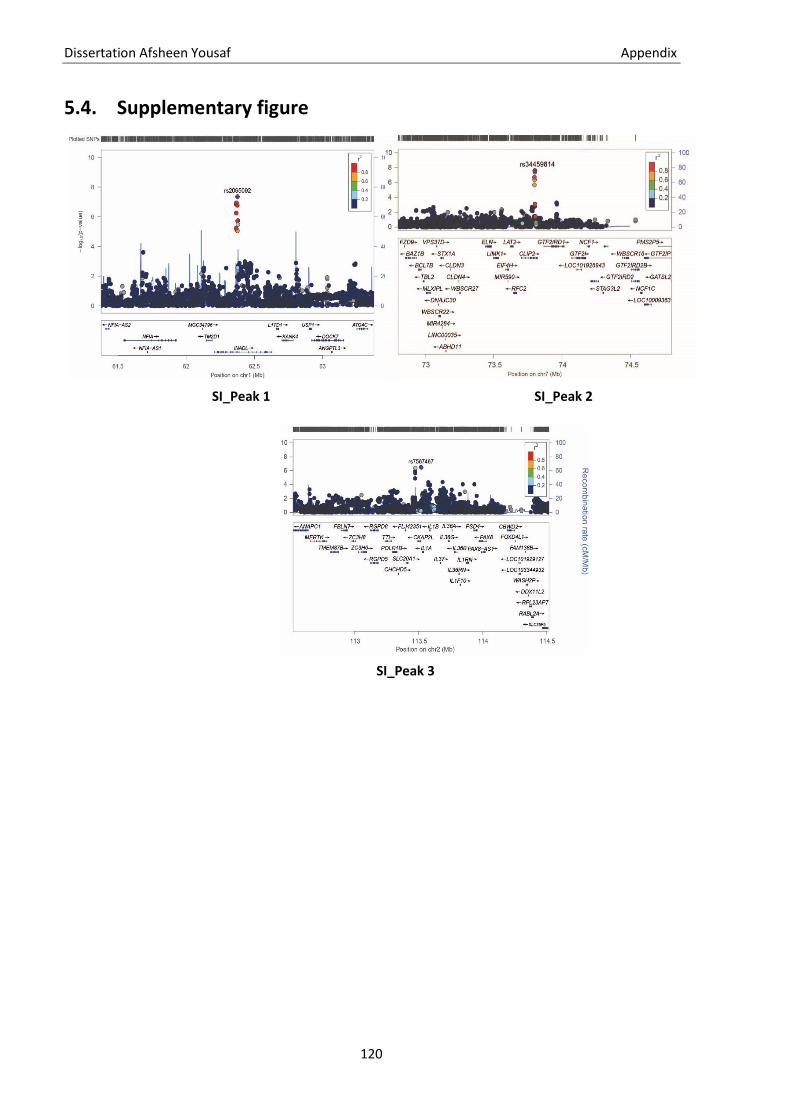
Dissertation Afsheen Yousaf Appendix
120
Supplementary figure 5.4.
SI_Peak 3
SI_Peak 1 SI_Peak 2
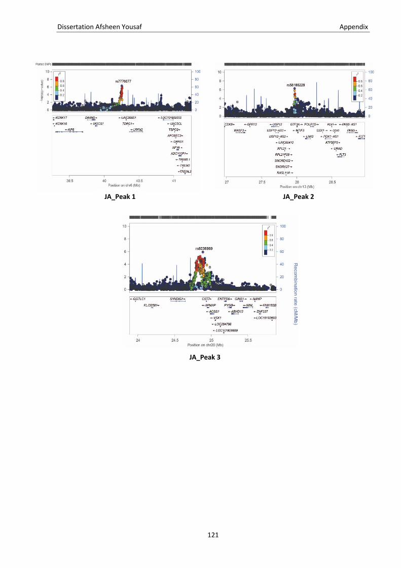
Dissertation Afsheen Yousaf Appendix
121
JA_Peak 3
JA_Peak 1 JA_Peak 2
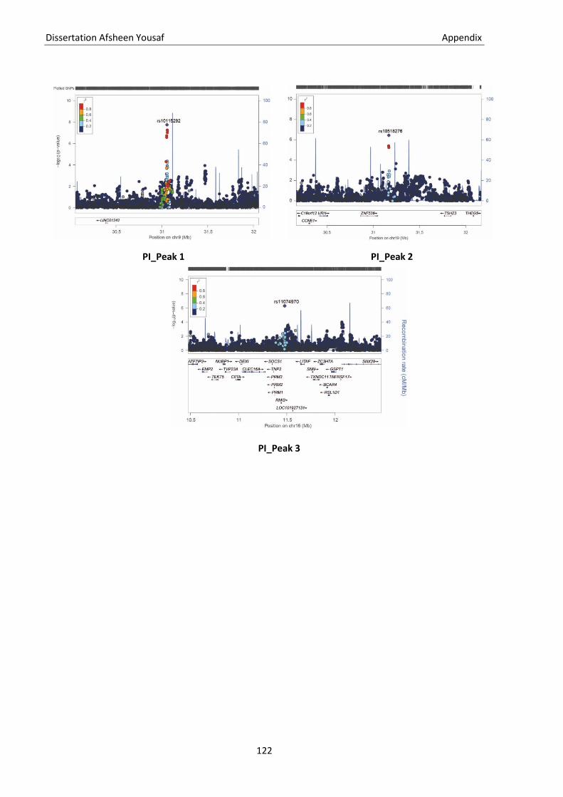
Dissertation Afsheen Yousaf Appendix
122
PI_Peak 1 PI_Peak 2
PI_Peak 3
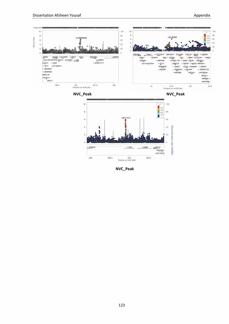
Dissertation Afsheen Yousaf Appendix
123
NVC_Peak
1
NVC_Peak
2
NVC_Peak
3
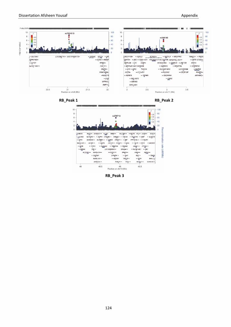
Dissertation Afsheen Yousaf Appendix
124
RB_Peak 1 RB_Peak 2
RB_Peak 3
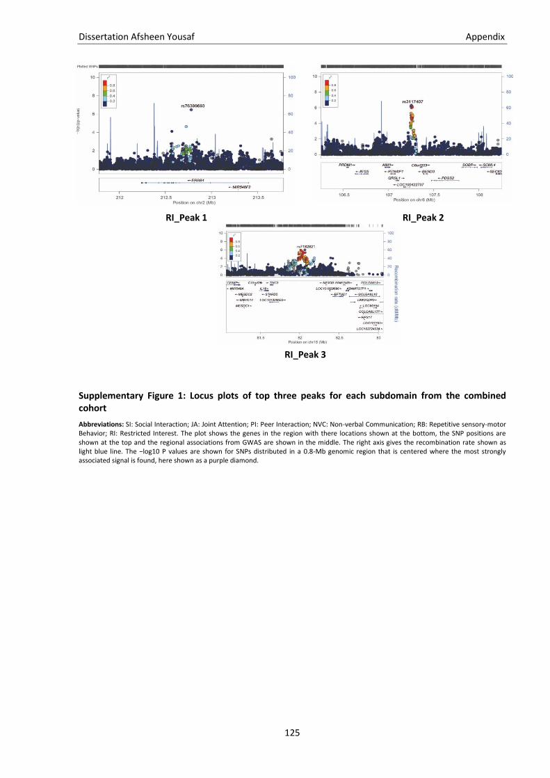
Dissertation Afsheen Yousaf Appendix
125
Supplementary Figure 1: Locus plots of top three peaks for each subdomain from the combined cohort
Abbreviations: SI: Social Interaction; JA: Joint Attention; PI: Peer Interaction; NVC: Non-verbal Communication; RB: Repetitive sensory-motor Behavior; RI: Restricted Interest. The plot shows the genes in the region with there locations shown at the bottom, the SNP positions are shown at the top and the regional associations from GWAS are shown in the middle. The right axis gives the recombination rate shown as light blue line. The −log10 P values are shown for SNPs distributed in a 0.8-Mb genomic region that is centered where the most strongly associated signal is found, here shown as a purple diamond.
RI_Peak 1 RI_Peak 2
RI_Peak 3

Dissertation Afsheen Yousaf Appendix
126
Dissertation Afsheen Yousaf References
127
6. References
1 Torrico B, Chiocchetti AG, Bacchelli E, Trabetti E, Hervas A, Franke B et al. Lack of replication of previous autism spectrum disorder GWAS hits in European populations. Autism Research 2016.
2 Chiocchetti AG, Yousaf A, Bour HS, Haslinger D, Waltes R, Duketis E et al. Common functional variants of the glutamatergic system in Autism spectrum disorder with high and low intellectual abilities. Journal of Neural Transmission (Vienna, Austria 1996) 2018; 125: 259–271.
3 Haslinger D, Waltes R, Yousaf A, Lindlar S, Schneider I, Lim CK et al. Loss of the Chr16p11.2 ASD candidate gene QPRT leads to aberrant neuronal differentiation in the SH-SY5Y neuronal cell model. Molecular Autism 2018; 9: 56.
4 Kang HJ, Kawasawa YI, Cheng F, Zhu Y, Xu X, Li M et al. Spatio-temporal transcriptome of the human brain. Nature 2011; 478: 483–489.
5 Barnett JH, Smoller JW. The genetics of bipolar disorder. Neuroscience 2009; 164: 331–343.
6 Faraone SV, Larsson H. Genetics of attention deficit hyperactivity disorder. Molecular Psychiatry 2019; 24: 562–575.
7 Hilker R, Helenius D, Fagerlund B, Skytthe A, Christensen K, Werge TM et al. Heritability of Schizophrenia and Schizophrenia Spectrum Based on the Nationwide Danish Twin Register. Biological Psychiatry 2018; 83: 492–498.
8 Sandin S, Lichtenstein P, Kuja-Halkola R, Hultman C, Larsson H, Reichenberg A. The Heritability of Autism Spectrum Disorder. JAMA 2017; 318: 1182–1184.
9 Gondro C, Porto-Neto LR, Lee SH. SNPQC—an R pipeline for quality control of Illumina SNP genotyping array data. Animal Genetics 2014; 45: 758–761.
10 Hibar DP, Stein JL, Renteria ME, Arias-Vasquez A, Desrivières S, Jahanshad N et al. Common genetic variants influence human subcortical brain structures. Nature 2015; 520: 224–229.
11 Kanterakis A, Deelen P, van Dijk F, Byelas H, Dijkstra M, Swertz MA. Molgenis-impute: Imputation pipeline in a box. BMC Research Notes 2015; 8: 359.
12 Muñiz-Fernandez F, Carreño-Torres A, Morcillo-Suarez C, Navarro A. Genome-wide association studies pipeline (GWASpi): A desktop application for genome-wide SNP analysis and management. Bioinformatics (Oxford, England) 2011; 27: 1871–1872.
13 Ripke S, Thomas B. Ricopili: Tool for visualizing regions of interest in selected GWAS data sets., 2011. https://data.broadinstitute.org/mpg/ricopili/ (accessed 8 Mar 2018).
14 Emery and Rimoin’s principles and practice of medical genetics and genomics: Foundations. Academic Press is an imprint of Elsevier: London, U.K, 2019.
15 Principles and practice of sleep medicine. Elsevier: Philadelphia, PA, 2017.
16 Lee H-S, Kim Y, Park T. New Common and Rare Variants Influencing Metabolic Syndrome and Its Individual Components in a Korean Population. Scientific Reports 2018; 8: 5701.
17 Lehne B, Lewis CM, Schlitt T. From SNPs to genes: disease association at the gene level. PLoS ONE 2011; 6: e20133.
18 Chakravarti A. To a future of genetic medicine. Nature 2001; 409: 822–823.
19 Auton A, Brooks LD, Durbin RM, Garrison EP, Kang HM, Korbel JO et al. A global reference for human genetic variation. Nature 2015; 526: 68–74.
20 Botstein D, Risch N. Discovering genotypes underlying human phenotypes: past successes for mendelian disease, future approaches for complex disease. Nature Genetics 2003; 33 Suppl: 228–237.
21 Cantor CR. The use of genetic SNPs as new diagnostic markers in preventive medicine. Annals of the New York Academy of Sciences 2005; 1055: 48–57.
Dissertation Afsheen Yousaf References
128
22 Jiao Y, Chen R, Ke X, Cheng L, Chu K, Lu Z et al. Single nucleotide polymorphisms predict symptom severity of autism spectrum disorder. Journal of Autism and Developmental Disorders 2012; 42: 971–983.
23 Yang Y, Wang W, Liu G, Yu Y, Liao M. Association of single nucleotide polymorphism rs3803662 with the risk of breast cancer. Scientific Reports 2016; 6: 29008.
24 Franke A, McGovern DPB, Barrett JC, Wang K, Radford-Smith GL, Ahmad T et al. Genome-wide meta-analysis increases to 71 the number of confirmed Crohn’s disease susceptibility loci. Nature Genetics 2010; 42: 1118–1125.
25 Flannick J, Florez JC. Type 2 diabetes: genetic data sharing to advance complex disease research. Nature Reviews. Genetics 2016; 17: 535–549.
26 Purcell SM, Wray NR, Stone JL, Visscher PM, O’Donovan MC, Sullivan PF et al. Common polygenic variation contributes to risk of schizophrenia and bipolar disorder. Nature 2009; 460: 748–752.
27 Feuk L, Carson AR, Scherer SW. Structural variation in the human genome. Nature Reviews. Genetics 2006; 7: 85–97.
28 Marshall CR, Noor A, Vincent JB, Lionel AC, Feuk L, Skaug J et al. Structural variation of chromosomes in autism spectrum disorder. American Journal of Human Genetics 2008; 82: 477–488.
29 Green EK, Rees E, Walters JTR, Smith K-G, Forty L, Grozeva D et al. Copy number variation in bipolar disorder. Molecular Psychiatry 2016; 21: 89–93.
30 Marshall CR, Howrigan DP, Merico D, Thiruvahindrapuram B, Wu W, Greer DS et al. Contribution of copy number variants to schizophrenia from a genome-wide study of 41,321 subjects, 49.
31 Kumaran M, Cass CE, Graham K, Mackey JR, Hubaux R, Lam W et al. Germline copy number variations are associated with breast cancer risk and prognosis. Scientific Reports 2017; 7: 14621.
32 Constantino JN, Todd RD. Autistic traits in the general population: A twin study. Archives of General Psychiatry 2003; 60: 524–530.
33 Ronald A, Hoekstra RA. Autism spectrum disorders and autistic traits: A decade of new twin studies. American journal of medical genetics. Part B, Neuropsychiatric genetics the official publication of the International Society of Psychiatric Genetics 2011; 156: 255–274.
34 Bölte S, Poustka F. Diagnostische Beobachtungsskala für Autistische Störungen (ADOS): Erste Ergebnisse zur Zuverlässigkeit und Gültigkeit. Zeitschrift für Kinder- und Jugendpsychiatrie und Psychotherapie 2004; 32: 45–50.
35 LaFramboise T. Single nucleotide polymorphism arrays: a decade of biological, computational and technological advances. Nucleic Acids Research 2009; 37: 4181–4193.
36 Illumina Inc. SNP genotyping.
37 Gunderson KL, Steemers FJ, Lee G, Mendoza LG, Chee MS. A genome-wide scalable SNP genotyping assay using microarray technology. Nature Genetics 2005; 37: 549–554.
38 Bush WS, Moore JH. Chapter 11: Genome-wide association studies. PLoS Computational Biology 2012; 8: e1002822.
39 Kermani BG. Artificial intelligence and global normalization methods for genotyping(20060224529).
40 Teo YY, Inouye M, Small KS, Gwilliam R, Deloukas P, Kwiatkowski DP et al. A genotype calling algorithm for the Illumina BeadArray platform. Bioinformatics (Oxford, England) 2007; 23: 2741–2746.
41 Kumar S, Banks TW, Cloutier S. SNP Discovery through Next-Generation Sequencing and Its Applications. International Journal of Plant Genomics 2012; 2012: 831460.
Dissertation Afsheen Yousaf References
129
42 Nielsen R, Paul JS, Albrechtsen A, Song YS. Genotype and SNP calling from next-generation sequencing data. Nature reviews. Genetics 2011; 12: 443–451.
43 Ritchie ME, Phipson B, Di Wu, Hu Y, Law CW, Shi W et al. limma powers differential expression analyses for RNA-sequencing and microarray studies. Nucleic Acids Research 2015; 43: e47.
44 Amin SB, Shah PK, Yan A, Adamia S, Minvielle S, Avet-Loiseau H et al. The dChip survival analysis module for microarray data. BMC Bioinformatics 2011; 12: 72.
45 Eijssen LMT, Jaillard M, Adriaens ME, Gaj S, Groot PJ de, Müller M et al. User-friendly solutions for microarray quality control and pre-processing on ArrayAnalysis.org. Nucleic Acids Research 2013; 41: W71-6.
46 Emig D, Salomonis N, Baumbach J, Lengauer T, Conklin BR, Albrecht M. AltAnalyze and DomainGraph: analyzing and visualizing exon expression data. Nucleic Acids Research 2010; 38: W755-62.
47 Xu G, Strathearn L, Liu B, Bao W. Prevalence of Autism Spectrum Disorder Among US Children and Adolescents, 2014-2016. JAMA 2018; 319: 81–82.
48 Elsabbagh M, Divan G, Koh Y-J, Kim YS, Kauchali S, Marcín C et al. Global prevalence of autism and other pervasive developmental disorders. Autism research official journal of the International Society for Autism Research 2012; 5: 160–179.
49 Lord C, Rutter M, Le Couteur A. Autism Diagnostic Interview-Revised: A revised version of a diagnostic interview for caregivers of individuals with possible pervasive developmental disorders. Journal of Autism and Developmental Disorders 1994; 24: 659–685.
50 World Health Organization. ICD-10: international statistical classification of diseases and related health problems: 10th revision: Geneva, 1992.
51 GUZE SB. Diagnostic and Statistical Manual of Mental Disorders, 4th ed. (DSM-IV), 152, 1995.
52 Kim SH, Thurm A, Shumway S, Lord C. Multisite study of new autism diagnostic interview-revised (ADI-R) algorithms for toddlers and young preschoolers. Journal of Autism and Developmental Disorders 2013; 43: 1527–1538.
53 Lord C, Rutter M, Goode S, Heemsbergen J, Jordan H, Mawhood L et al. Autism diagnostic observation schedule: a standardized observation of communicative and social behavior. Journal of Autism and Developmental Disorders 1989; 19: 185–212.
54 Bailey A, Le Couteur A, Gottesman I, Bolton P, Simonoff E, Yuzda E et al. Autism as a strongly genetic disorder: evidence from a British twin study. Psychological Medicine 1995; 25: 63–77.
55 Tick B, Bolton P, Happé F, Rutter M, Rijsdijk F. Heritability of autism spectrum disorders: A meta-analysis of twin studies. Journal of Child Psychology and Psychiatry 2016; 57: 585–595.
56 Bai D, Yip BHK, Windham GC, Sourander A, Francis R, Yoffe R et al. Association of Genetic and Environmental Factors With Autism in a 5-Country Cohort. JAMA psychiatry 2019.
57 Grove J, Ripke S, Als TD, Mattheisen M, Walters RK, Won H et al. Identification of common genetic risk variants for autism spectrum disorder. Nature Genetics 2019; 51: 431–444.
58 Leblond CS, Cliquet F, Carton C, Huguet G, Mathieu A, Kergrohen T et al. Both rare and common genetic variants contribute to autism in the Faroe Islands. NPJ Genomic Medicine 2019; 4: 1.
59 Huguet G, Bourgeron T. Genetic Causes of Autism Spectrum Disorders.
60 Bourgeron T. From the genetic architecture to synaptic plasticity in autism spectrum disorder. Nature reviews. Neuroscience 2015; 16: 551–563.
61 Sun H-Y, Ji F-Q, Fu L-Y, Wang Z-Y, Zhang H-Y. Structural and energetic analyses of SNPs in drug targets and implications for drug therapy. Journal of Chemical Information and Modeling 2013; 53: 3343–3351.
62 Gaugler T, Klei L, Sanders SJ, Bodea CA, Goldberg AP, Lee AB et al. Most genetic risk for autism resides with common variation. Nature Genetics 2014; 46: 881–885.

Dissertation Afsheen Yousaf References
130
63 Sayad A, Noroozi R, Omrani MD, Taheri M, Ghafouri-Fard S. Retinoic acid-related orphan receptor alpha (RORA) variants are associated with autism spectrum disorder. Metabolic Brain Disease 2017; 32: 1595–1601.
64 Freitag CM, Staal W, Klauck SM, Duketis E, Waltes R. Genetics of autistic disorders: Review and clinical implications. European Child & Adolescent Psychiatry 2010; 19: 169–178.
65 Toma C, Pierce KD, Shaw AD, Heath A, Mitchell PB, Schofield PR et al. Comprehensive cross-disorder analyses of CNTNAP2 suggest it is unlikely to be a primary risk gene for psychiatric disorders. PLoS Genetics 2018; 14: e1007535.
66 Chiocchetti AG, Kopp M, Waltes R, Haslinger D, Duketis E, Jarczok TA et al. Variants of the CNTNAP2 5′ promoter as risk factors for autism spectrum disorders: a genetic and functional approach. Molecular Psychiatry 2015; 20: 839–849.
67 Noroozi R, Taheri M, Ghafouri-Fard S, Bidel Z, Omrani MD, Moghaddam AS et al. Meta-analysis of GABRB3 Gene Polymorphisms and Susceptibility to Autism Spectrum Disorder. Journal of Molecular Neuroscience MN 2018; 65: 432–437.
68 Sanders SJ, Ercan-Sencicek AG, Hus V, Luo R, Murtha MT, Moreno-De-Luca D et al. Multiple recurrent de novo CNVs, including duplications of the 7q11.23 Williams syndrome region, are strongly associated with autism. Neuron 2011; 70: 863–885.
69 Morrow EM, Yoo S-Y, Flavell SW, Kim T-K, Lin Y, Hill RS et al. Identifying autism loci and genes by tracing recent shared ancestry. Science (New York, N.Y.) 2008; 321: 218–223.
70 Xu J, Zwaigenbaum L, Szatmari P, Scherer S. Molecular Cytogenetics of Autism. CG 2004; 5: 347–364.
71 Sebat J, Lakshmi B, Malhotra D, Troge J, Lese-Martin C, Walsh T et al. Strong association of de novo copy number mutations with autism. Science (New York, N.Y.) 2007; 316: 445–449.
72 Glessner JT, Wang K, Cai G, Korvatska O, Kim CE, Wood S et al. Autism genome-wide copy number variation reveals ubiquitin and neuronal genes. Nature 2009; 459: 569–573.
73 Iossifov I, O’Roak BJ, Sanders SJ, Ronemus M, Krumm N, Levy D et al. The contribution of de novo coding mutations to autism spectrum disorder. Nature 2014; 515: 216–221.
74 Ma D, Salyakina D, Jaworski JM, Konidari I, Whitehead PL, Andersen AN et al. A genome-wide association study of autism reveals a common novel risk locus at 5p14.1. Annals of Human Genetics 2009; 73: 263–273.
75 Devlin B, Melhem N, Roeder K. Do common variants play a role in risk for autism? Evidence and theoretical musings. Brain Research 2011; 1380: 78–84.
76 The Autism Spectrum Disorders Working Group of The Psychiatric Genomics Consortium. Meta-analysis of GWAS of over 16,000 individuals with autism spectrum disorder highlights a novel locus at 10q24.32 and a significant overlap with schizophrenia. Molecular Autism 2017; 8: 21.
77 Folstein S, Rutter M. Infantile autism: a genetic study of 21 twin pairs. Journal of Child Psychology and Psychiatry 1977; 18: 297–321.
78 Ronald A, Happé F, Bolton P, Butcher LM, Price TS, Wheelwright S et al. Genetic heterogeneity between the three components of the autism spectrum: a twin study. Journal of the American Academy of Child and Adolescent Psychiatry 2006; 45: 691–699.
79 Ronald A, Happé F, Plomin R. The genetic relationship between individual differences in social and nonsocial behaviours characteristic of autism. Developmental Science 2005; 8: 444–458.
80 Rosenberg RE, Law JK, Yenokyan G, McGready J, Kaufmann WE, Law PA. Characteristics and concordance of autism spectrum disorders among 277 twin pairs. Archives of Pediatrics & Adolescent Medicine 2009; 163: 907–914.
81 Sandin S, Lichtenstein P, Kuja-Halkola R, Larsson H, Hultman CM, Reichenberg A. The familial risk of autism. JAMA 2014; 311: 1770–1777.
Dissertation Afsheen Yousaf References
131
82 Morton NE. Logarithm of odds (lods) for linkage in complex inheritance. Proceedings of the National Academy of Sciences of the United States of America 1996; 93: 3471–3476.
83 Liu X-Q, Paterson AD, Szatmari P. Genome-wide linkage analyses of quantitative and categorical autism subphenotypes. Biological Psychiatry 2008; 64: 561–570.
84 Liu X-Q, Georgiades S, Duku E, Thompson A, Devlin B, Cook EH et al. Identification of genetic loci underlying the phenotypic constructs of autism spectrum disorders. Journal of the American Academy of Child and Adolescent Psychiatry 2011; 50: 687-696.e13.
85 Weiss LA, Arking DE, Daly MJ, Chakravarti A. A genome-wide linkage and association scan reveals novel loci for autism. Nature 2009; 461: 802–808.
86 Price AL, Spencer CCA, Donnelly P. Progress and promise in understanding the genetic basis of common diseases. Proceedings. Biological Sciences 2015; 282: 20151684.
87 McCarthy MI, Abecasis GR, Cardon LR, Goldstein DB, Little J, Ioannidis JPA et al. Genome-wide association studies for complex traits: consensus, uncertainty and challenges. Nature Reviews Genetics 2008; 9: 356–369.
88 Benjamini Y, Hochberg Y. Controlling the False Discovery Rate: A Practical and Powerful Approach to Multiple Testing. Journal of the Royal Statistical Society. Series B (Methodological) 1995; 57: 289–300.
89 NEYMAN J, PEARSON ES. ON THE USE AND INTERPRETATION OF CERTAIN TEST CRITERIA FOR PURPOSES OF STATISTICAL INFERENCE PART I. Biometrika 1928; 20A: 175–240.
90 Zhang L, Liu L, Wen Y, Ma M, Cheng S, Yang J et al. Genome-wide association study and identification of chromosomal enhancer maps in multiple brain regions related to autism spectrum disorder. Autism research official journal of the International Society for Autism Research 2019; 12: 26–32.
91 Poelmans G, Franke B, Pauls DL, Glennon JC, Buitelaar JK. AKAPs integrate genetic findings for autism spectrum disorders. Translational Psychiatry 2013; 3: e270.
92 Coon KD, Myers AJ, Craig DW, Webster JA, Pearson JV, Lince DH et al. A high-density whole-genome association study reveals that APOE is the major susceptibility gene for sporadic late-onset Alzheimer’s disease. The Journal of Clinical Psychiatry 2007; 68: 613–618.
93 Fung H-C, Scholz S, Matarin M, Simón-Sánchez J, Hernandez D, Britton A et al. Genome-wide genotyping in Parkinson’s disease and neurologically normal controls: first stage analysis and public release of data. The Lancet. Neurology 2006; 5: 911–916.
94 Matarín M, Brown WM, Scholz S, Simón-Sánchez J, Fung H-C, Hernandez D et al. A genome-wide genotyping study in patients with ischaemic stroke: initial analysis and data release. The Lancet. Neurology 2007; 6: 414–420.
95 Schizophrenia working group of the Psychiatric Genomics Consortium. Biological insights from 108 schizophrenia-associated genetic loci. Nature 2014; 511: 421–427.
96 Wang K, Zhang H, Ma D, Bucan M, Glessner JT, Abrahams BS et al. Common genetic variants on 5p14.1 associate with autism spectrum disorders. Nature 2009; 459: 528–533.
97 Anney R, Klei L, Pinto D, Regan R, Conroy J, Magalhaes TR et al. A genome-wide scan for common alleles affecting risk for autism. Human Molecular Genetics 2010; 19: 4072–4082.
98 Connolly JJ, Glessner JT, Hakonarson H. A genome-wide association study of autism incorporating autism diagnostic interview-revised, autism diagnostic observation schedule, and social responsiveness scale. Child Development 2013; 84: 17–33.
99 Cross-Disorder Group of the Psychiatric Genomics Consortium. Identification of risk loci with shared effects on five major psychiatric disorders: A genome-wide analysis. THE LANCET 2013; 381: 1371–1379.
Dissertation Afsheen Yousaf References
132
100 Cantor RM, Navarro L, Won H, Walker RL, Lowe JK, Geschwind DH. ASD restricted and repetitive behaviors associated at 17q21.33: genes prioritized by expression in fetal brains. Molecular Psychiatry 2018; 23: 993–1000.
101 Zarrei M, Macdonald JR, Merico D, Scherer SW. A copy number variation map of the human genome. Nature reviews. Genetics 2015; 16: 172–183.
102 Pinto D, Darvishi K, Shi X, Rajan D, Rigler D, Fitzgerald T et al. Comprehensive assessment of array-based platforms and calling algorithms for detection of copy number variants. Nature biotechnology 2011; 29: 512–520.
103 Kushima I, Aleksic B, Nakatochi M, Shimamura T, Okada T, Uno Y et al. Comparative Analyses of Copy-Number Variation in Autism Spectrum Disorder and Schizophrenia Reveal Etiological Overlap and Biological Insights. Cell reports 2018; 24: 2838–2856.
104 Dajani R, Li J, Wei Z, Glessner JT, Chang X, Cardinale CJ et al. CNV Analysis Associates AKNAD1 with Type-2 Diabetes in Jordan Subpopulations. Scientific reports 2015; 5: 13391.
105 Marshall CR, Howrigan DP, Merico D, Thiruvahindrapuram B, Wu W, Greer DS et al. Contribution of copy number variants to schizophrenia from a genome-wide study of 41,321 subjects. Nature Genetics 2017; 49: 27–35.
106 Pinto D, Pagnamenta AT, Klei L, Anney R, Merico D, Regan R et al. Functional impact of global rare copy number variation in autism spectrum disorders. Nature 2010; 466: 368–372.
107 Levy D, Ronemus M, Yamrom B, Lee Y-h, Leotta A, Kendall J et al. Rare de novo and transmitted copy-number variation in autistic spectrum disorders. Neuron 2011; 70: 886–897.
108 Kim H-G, Kishikawa S, Higgins AW, Seong I-S, Donovan DJ, Shen Y et al. Disruption of neurexin 1 associated with autism spectrum disorder, 2008.
109 Roohi J, Montagna C, Tegay DH, Palmer LE, DeVincent C, Pomeroy JC et al. Disruption of contactin 4 in three subjects with autism spectrum disorder. Journal of Medical Genetics 2009; 46: 176–182.
110 Moessner R, Marshall CR, Sutcliffe JS, Skaug J, Pinto D, Vincent J et al. Contribution of SHANK3 mutations to autism spectrum disorder. American Journal of Human Genetics 2007; 81: 1289–1297.
111 Szatmari P, Paterson AD, Zwaigenbaum L, Roberts W, Brian J, Liu X-Q et al. Mapping autism risk loci using genetic linkage and chromosomal rearrangements. Nature Genetics 2007; 39: 319–328.
112 Manning MA, Cassidy SB, Clericuzio C, Cherry AM, Schwartz S, Hudgins L et al. Terminal 22q deletion syndrome: a newly recognized cause of speech and language disability in the autism spectrum. Pediatrics 2004; 114: 451–457.
113 Kumar RA, KaraMohamed S, Sudi J, Conrad DF, Brune C, Badner JA et al. Recurrent 16p11.2 microdeletions in autism. Human Molecular Genetics 2008; 17: 628–638.
114 Yin C-L, Chen H-I, Li L-H, Chien Y-L, Liao H-M, Chou MC et al. Genome-wide analysis of copy number variations identifies PARK2 as a candidate gene for autism spectrum disorder. Molecular Autism 2016; 7: 23.
115 Talkowski ME, Rosenfeld JA, Blumenthal I, Pillalamarri V, Chiang C, Heilbut A et al. Sequencing chromosomal abnormalities reveals neurodevelopmental loci that confer risk across diagnostic boundaries. Cell 2012; 149: 525–537.
116 Xu B, Roos JL, Dexheimer P, Boone B, Plummer B, Levy S et al. Exome sequencing supports a de novo mutational paradigm for schizophrenia. Nature Genetics 2011; 43: 864–868.
117 Cai N, Bigdeli T, Kretzschmar Wea. Sparse whole-genome sequencing identifies two loci for major depressive disorder. Nature 2015; 523: 588–591.

Dissertation Afsheen Yousaf References
133
118 Sanders SJ, Murtha MT, Gupta AR, Murdoch JD, Raubeson MJ, Willsey AJ et al. De novo mutations revealed by whole-exome sequencing are strongly associated with autism. Nature 2012; 485: 237–241.
119 Rubeis S de, He X, Goldberg AP, Poultney CS, Samocha K, Cicek AE et al. Synaptic, transcriptional and chromatin genes disrupted in autism. Nature 2014; 515: 209–215.
120 Dong S, Walker MF, Carriero NJ, DiCola M, Willsey AJ, Ye AY et al. De novo insertions and deletions of predominantly paternal origin are associated with autism spectrum disorder. Cell Reports 2014; 9: 16–23.
121 Chen L, Page GP, Mehta T, Feng R, Cui X. Single nucleotide polymorphisms affect both cis- and trans-eQTLs. Genomics 2009; 93: 501–508.
122 Cookson W, Liang L, Abecasis G, Moffatt M, Lathrop M. Mapping complex disease traits with global gene expression. Nature Reviews. Genetics 2009; 10: 184–194.
123 Cheng Y, Quinn JF, Weiss LA. An eQTL mapping approach reveals that rare variants in the SEMA5A regulatory network impact autism risk. Human Molecular Genetics 2013; 22: 2960–2972.
124 O’Brien HE, Hannon E, Hill MJ, Toste CC, Robertson MJ, Morgan JE et al. Expression quantitative trait loci in the developing human brain and their enrichment in neuropsychiatric disorders. Genome Biology 2018; 19: 194.
125 Bhalala OG, Nath AP, Inouye M, Sibley CR. Identification of expression quantitative trait loci associated with schizophrenia and affective disorders in normal brain tissue. PLoS Genetics 2018; 14: e1007607.
126 Davis LK, Gamazon ER, Kistner-Griffin E, Badner JA, Liu C, Cook EH et al. Loci nominally associated with autism from genome-wide analysis show enrichment of brain expression quantitative trait loci but not lymphoblastoid cell line expression quantitative trait loci. Molecular Autism 2012; 3: 3.
127 He X, Fuller CK, Song Y, Meng Q, Zhang B, Yang X et al. Sherlock: detecting gene-disease associations by matching patterns of expression QTL and GWAS. American Journal of Human Genetics 2013; 92: 667–680.
128 Yin X, Cheng H, Lin Y, Fan X, Cui Y, Zhou F et al. Five regulatory genes detected by matching signatures of eQTL and GWAS in psoriasis. Journal of Dermatological Science 2014; 76: 139–142.
129 Yang C-P, Li X, Wu Y, Shen Q, Zeng Y, Xiong Q et al. Comprehensive integrative analyses identify GLT8D1 and CSNK2B as schizophrenia risk genes. Nature communications 2018; 9: 838.
130 Lord C, Storoschuk S, Rutter M, Pickles A. Using the ADI-R to diagnose autism in preschool children. Infant Ment. Health J. 1993; 14: 234–252.
131 Hus V, Lord C. Effects of child characteristics on the Autism Diagnostic Interview-Revised: implications for use of scores as a measure of ASD severity. Journal of Autism and Developmental Disorders 2013; 43: 371–381.
132 Akshoomoff N, Corsello C, Schmidt H. The Role of the Autism Diagnostic Observation Schedule in the Assessment of Autism Spectrum Disorders in School and Community Settings. The California School Psychologist CASP 2006; 11: 7–19.
133 Anderson CA, Pettersson FH, Clarke GM, Cardon LR, Morris AP, Zondervan KT. Data quality control in genetic case-control association studies. Nature Protocols 2010; 5: 1564–1573.
134 Illumina Inc. Improved Cluster Generation with Gentrain2.Technical Note: DNA Analysis., 2009. https://www.illumina.com/documents/products/technotes/technote_gentrain2.pdf (accessed 17 Apr 2018).
135 Band G, Marchini J. QCTOOL.
Dissertation Afsheen Yousaf References
134
136 D’Angelo GM, Kamboh MI, Feingold E. A Likelihood-Based Approach for Missing Genotype Data. Human Heredity 2010; 69: 171–183.
137 Clayton DG, Walker NM, Smyth DJ, Pask R, Cooper JD, Maier LM et al. Population structure, differential bias and genomic control in a large-scale, case-control association study. Nature Genetics 2005; 37: 1243–1246.
138 Howie B, Fuchsberger C, Stephens M, Marchini J, Abecasis GR. Fast and accurate genotype imputation in genome-wide association studies through pre-phasing. Nature Genetics 2012; 44: 955–959.
139 Stephens M, Scheet P. Accounting for decay of linkage disequilibrium in haplotype inference and missing-data imputation. American Journal of Human Genetics 2005; 76: 449–462.
140 Scheet P, Stephens M. A fast and flexible statistical model for large-scale population genotype data: applications to inferring missing genotypes and haplotypic phase. American Journal of Human Genetics 2006; 78: 629–644.
141 Kimmel G, Shamir R. GERBIL: Genotype resolution and block identification using likelihood. Proceedings of the National Academy of Sciences of the United States of America 2005; 102: 158–162.
142 Lemieux Perreault L-P, Legault M-A, Asselin G, Dubé M-P. genipe: An automated genome-wide imputation pipeline with automatic reporting and statistical tools. Bioinformatics (Oxford, England) 2016; 32: 3661–3663.
143 Chen J, Lippold D, Frank J, Rayner W, Meyer-Lindenberg A, Schwarz E. Gimpute: An efficient genetic data imputation pipeline. Bioinformatics (Oxford, England) 2018.
144 Purcell S, Neale B, Todd-Brown K, Thomas L, Ferreira MAR, Bender D et al. PLINK: A tool set for whole-genome association and population-based linkage analyses. American Journal of Human Genetics 2007; 81: 559–575.
145 Delaneau O, Marchini J, Zagury J-F. A linear complexity phasing method for thousands of genomes. Nature Methods 2011; 9: 179–181.
146 Das S, Forer L, Schonherr S, Sidore C, Locke AE, Kwong A et al. Next-generation genotype imputation service and methods. Nature Genetics 2016; 48: 1284–1287.
147 Browning BL, Browning SR. Genotype Imputation with Millions of Reference Samples. American Journal of Human Genetics 2016; 98: 116–126.
148 Duncan LE, Ostacher M, Ballon J. How genome-wide association studies (GWAS) made traditional candidate gene studies obsolete. Neuropsychopharmacology Official Publication of the American College of Neuropsychopharmacology 2019; 44: 1518–1523.
149 Grimm DG, Roqueiro D, Salomé PA, Kleeberger S, Greshake B, Zhu W et al. easyGWAS: A Cloud-Based Platform for Comparing the Results of Genome-Wide Association Studies. The Plant Cell 2017; 29: 5–19.
150 Gogarten SM, Bhangale T, Conomos MP, Laurie CA, McHugh CP, Painter I et al. GWASTools: an R/Bioconductor package for quality control and analysis of genome-wide association studies. Bioinformatics (Oxford, England) 2012; 28: 3329–3331.
151 Wray NR, Lee SH, Mehta D, Vinkhuyzen AAE, Dudbridge F, Middeldorp CM. Research review: Polygenic methods and their application to psychiatric traits. Journal of Child Psychology and Psychiatry, and Allied Disciplines 2014; 55: 1068–1087.
152 Wang L, Jia P, Wolfinger RD, Chen X, Zhao Z. Gene set analysis of genome-wide association studies: methodological issues and perspectives. Genomics 2011; 98: 1–8.
153 Leeuw CA de, Mooij JM, Heskes T, Posthuma D. MAGMA: Generalized gene-set analysis of GWAS data. PLoS Computational Biology 2015; 11: e1004219.
Dissertation Afsheen Yousaf References
135
154 Mishra A, Macgregor S. VEGAS2: Software for More Flexible Gene-Based Testing. Twin Research and Human Genetics the Official Journal of the International Society for Twin Studies 2015; 18: 86–91.
155 Lee PH, O’Dushlaine C, Thomas B, Purcell SM. INRICH: Interval-based enrichment analysis for genome-wide association studies. Bioinformatics (Oxford, England) 2012; 28: 1797–1799.
156 Holmans P, Green EK, Pahwa JS, Ferreira MAR, Purcell SM, Sklar P et al. Gene ontology analysis of GWA study data sets provides insights into the biology of bipolar disorder. American Journal of Human Genetics 2009; 85: 13–24.
157 Liu JZ, McRae AF, Nyholt DR, Medland SE, Wray NR, Brown KM et al. A versatile gene-based test for genome-wide association studies. American Journal of Human Genetics 2010; 87: 139–145.
158 Segrè AV, Groop L, Mootha VK, Daly MJ, Altshuler D. Common inherited variation in mitochondrial genes is not enriched for associations with type 2 diabetes or related glycemic traits. PLoS Genetics 2010; 6.
159 Huang DW, Sherman BT, Tan Q, Collins JR, Alvord WG, Roayaei J et al. The DAVID Gene Functional Classification Tool: a novel biological module-centric algorithm to functionally analyze large gene lists. Genome Biology 2007; 8: R183.
160 Song GG, Lee YH. Pathway analysis of genome-wide association studies for Parkinson’s disease. Molecular Biology Reports 2013; 40: 2599–2607.
161 Mi H, Muruganujan A, Casagrande JT, Thomas PD. Large-scale gene function analysis with the PANTHER classification system. Nature Protocols 2013; 8: 1551–1566.
162 Zambon AC, Gaj S, Ho I, Hanspers K, Vranizan K, Evelo CT et al. GO-Elite: A flexible solution for pathway and ontology over-representation. Bioinformatics (Oxford, England) 2012; 28: 2209–2210.
163 Berument SK, Rutter M, Lord C, Pickles A, Bailey A. Autism screening questionnaire: diagnostic validity. The British Journal of Psychiatry the Journal of Mental Science 1999; 175: 444–451.
164 Lord C, Risi S, Lambrecht L, Cook EH, Leventhal BL, DiLavore PC et al. The autism diagnostic observation schedule-generic: A standard measure of social and communication deficits associated with the spectrum of autism. Journal of Autism and Developmental Disorders 2000; 30: 205–223.
165 Janca A, Ustün TB, Early TS, Sartorius N. The ICD-10 symptom checklist: A companion to the ICD-10 classification of mental and behavioural disorders. Social Psychiatry and Psychiatric Epidemiology 1993; 28: 239–242.
166 Poustka F, Lisch S, Rühl D, Sacher A, Schmötzer G, Werner K. The standardized diagnosis of autism, Autism Diagnostic Interview-Revised: Interrater reliability of the German form of the interview. Psychopathology 1996; 29: 145–153.
167 Rabbee N, Speed TP. A genotype calling algorithm for affymetrix SNP arrays. Bioinformatics (Oxford, England) 2006; 22: 7–12.
168 Stef van Buuren, Karin Groothuis-Oudshoorn. mice: Multivariate Imputation by Chained Equations in R 2011.
169 Azur MJ, Stuart EA, Frangakis C, Leaf PJ. Multiple imputation by chained equations: what is it and how does it work? International Journal of Methods in Psychiatric Research 2011; 20: 40–49.
170 RUBIN DB. Statistical Matching Using File Concatenation with Adjusted Weights and Multiple Imputations. Journal of Business & Economic Statistics 1986; 4: 87.
171 Horton NJ, Kleinman KP. Much ado about nothing: A comparison of missing data methods and software to fit incomplete data regression models. The American Statistician 2007; 61: 79–90.
Dissertation Afsheen Yousaf References
136
172 Frazier TW, Youngstrom EA, Kubu CS, Sinclair L, Rezai A. Exploratory and confirmatory factor analysis of the autism diagnostic interview-revised. Journal of Autism and Developmental Disorders 2008; 38: 474–480.
173 Tao Y, Gao H, Ackerman B, Guo W, Saffen D, Shugart YY. Evidence for contribution of common genetic variants within chromosome 8p21.2-8p21.1 to restricted and repetitive behaviors in autism spectrum disorders. BMC Genomics 2016; 17: 163.
174 Bölte S, Poustka F. Die Faktorenstruktur des Autismus Diagnostischen Interviews-Revision (ADI-R): Eine Untersuchung zur dimensionalen versus kategorialen Klassifikation autistischer Störungen. Zeitschrift für Kinder- und Jugendpsychiatrie und Psychotherapie 2001; 29: 221–229.
175 Barrett PT, Kline P. The observation to variable ratio in factor analysis. Personality Study and Group Behavior.
176 Aleamoni LM. The Relation of Sample Size to the Number of Variables in Using Factor Analysis Techniques. Educational and Psychological Measurement 1976; 36: 879–883.
177 Kaiser HF. An index of factorial simplicity, 39, 1974.
178 William Revelle. psych: Procedures for Psychological, Psychometric, and Personality Research, 2017.
179 Kaiser HF. The Application of Electronic Computers to Factor Analysis. Educational and Psychological Measurement 1960; 20: 141–151.
180 Thorndike RL. Who belongs in the family? Psychometrika 1953; 18: 267–276.
181 Anderson TW, Rubin H. Statistical Inference in Factor Analysis. Neyman, J., Ed., Proceedings of the Third Berkeley Symposium on Mathematical Statistics and Probability 1956; 5: 111–150.
182 Comrey AL. Factor-analytic methods of scale development in personality and clinical psychology. Journal of Consulting and Clinical Psychology 1988; 56: 754–761.
183 Guadagnoli E, Velicer WF. Relation of sample size to the stability of component patterns. Psychological Bulletin 1988; 103: 265–275.
184 Tabachnick BG, Fidell LS. Using multivariate statistics, 6th edn. Pearson Education: Boston, 2013.
185 Faul F, Erdfelder E, Buchner A, Lang A-G. Statistical power analyses using G*Power 3.1: Tests for correlation and regression analyses. Behavior Research Methods 2009; 41: 1149–1160.
186 Lam M, Awasthi S, Watson HJ, Goldstein J, Panagiotaropoulou G, Trubetskoy V et al. RICOPILI: Rapid Imputation for COnsortias PIpeLIne. Bioinformatics (Oxford, England) 2019.
187 Turner S, Armstrong LL, Bradford Y, Carlson CS, Crawford DC, Crenshaw AT et al. Quality control procedures for genome-wide association studies. Current Protocols in Human Genetics 2011; Chapter 1: Unit1.19.
188 Kido T, Sikora-Wohlfeld W, Kawashima M, Kikuchi S, Kamatani N, Patwardhan A et al. Are minor alleles more likely to be risk alleles? BMC Medical Genomics 2018; 11: 3.
189 Marees AT, Kluiver H de, Stringer S, Vorspan F, Curis E, Marie-Claire C et al. A tutorial on conducting genome-wide association studies: Quality control and statistical analysis. International Journal of methods in Psychiatric Research 2018; 27: e1608.
190 Rédei GP (ed). Encyclopedia of genetics, genomics, proteomics, and informatics, 3rd edn. Springer reference. Springer part of Springer Science + Business Media: Dordrecht, 2008.
191 Abbott S, Fairbanks DJ. Experiments on Plant Hybrids by Gregor Mendel. Genetics 2016; 204: 407–422.
192 Lowe JK, Maller JB, Pe’er I, Neale BM, Salit J, Kenny EE et al. Genome-wide association studies in an isolated founder population from the Pacific Island of Kosrae. PLoS Genetics 2009; 5: e1000365.
Dissertation Afsheen Yousaf References
137
193 Tyner C, Barber GP, Casper J, Clawson H, Diekhans M, Eisenhart C et al. The UCSC Genome Browser database: 2017 update. Nucleic Acids Research 2017; 45: D626-D634.
194 Verma SS, Andrade M de, Tromp G, Kuivaniemi H, Pugh E, Namjou-Khales B et al. Imputation and quality control steps for combining multiple genome-wide datasets. Front. Genet. 2014; 5.
195 Yang J, Lee SH, Goddard ME, Visscher PM. GCTA: A tool for genome-wide complex trait analysis. American Journal of Human Genetics 2011; 88: 76–82.
196 Euesden J, Lewis CM, O’Reilly PF. PRSice: Polygenic Risk Score software. Bioinformatics (Oxford, England) 2015; 31: 1466–1468.
197 Bentler PM. Comparative fit indexes in structural models. Psychological Bulletin 1990; 107: 238–246.
198 Hu L‐t, Bentler PM. Cutoff criteria for fit indexes in covariance structure analysis: Conventional criteria versus new alternatives. Structural Equation Modeling: A Multidisciplinary Journal 1999; 6: 1–55.
199 Browne MW, Cudeck R. Alternative Ways of Assessing Model Fit. Sociological Methods & Research 2016; 21: 230–258.
200 MacCallum RC, Browne MW, Sugawara HM. Power analysis and determination of sample size for covariance structure modeling. Psychological Methods 1996; 1: 130–149.
201 Lin S, Chakravarti A, Cutler DJ. Haplotype and missing data inference in nuclear families. Genome Research 2004; 14: 1624–1632.
202 Sicotte H, Proddutur N. EZimputer.
203 Lee SH, Ripke S, Neale BM, Faraone SV, Purcell SM, Perlis RH et al. Genetic relationship between five psychiatric disorders estimated from genome-wide SNPs. Nature Genetics 2013; 45: 984–994.
204 Freitag CM, Jensen K, Elsuni L, Sachse M, Herpertz-Dahlmann B, Schulte-Rüther M et al. Group-based cognitive behavioural psychotherapy for children and adolescents with ASD: the randomized, multicentre, controlled SOSTA-net trial. Journal of Child Psychology and Psychiatry, and Allied Disciplines 2016; 57: 596–605.
205 Shuster J, Perry A, Bebko J, Toplak ME. Review of factor analytic studies examining symptoms of autism spectrum disorders. Journal of Autism and Developmental Disorders 2014; 44: 90–110.
206 Stranger BE, Stahl EA, Raj T. Progress and promise of genome-wide association studies for human complex trait genetics. Genetics 2011; 187: 367–383.
207 Tadevosyan-Leyfer O, Dowd M, Mankoski R, Winklosky B, Putnam S, McGrath L et al. A principal components analysis of the Autism Diagnostic Interview-Revised. Journal of the American Academy of Child and Adolescent Psychiatry 2003; 42: 864–872.
208 Anzai N, Deval E, Schaefer L, Friend V, Lazdunski M, Lingueglia E. The multivalent PDZ domain-containing protein CIPP is a partner of acid-sensing ion channel 3 in sensory neurons. The Journal of Biological Chemistry 2002; 277: 16655–16661.
209 Kenny EM, Cormican P, Furlong S, Heron E, Kenny G, Fahey C et al. Excess of rare novel loss-of-function variants in synaptic genes in schizophrenia and autism spectrum disorders. Molecular Psychiatry 2014; 19: 872–879.
210 Klein-Tasman BP, Mervis CB. Autism Spectrum Symptomatology Among Children with Duplication 7q11.23 Syndrome. Journal of Autism and Developmental Disorders 2018; 48: 1982–1994.
211 Beunders G, Voorhoeve E, Golzio C, Pardo LM, Rosenfeld JA, Talkowski ME et al. Exonic deletions in AUTS2 cause a syndromic form of intellectual disability and suggest a critical role for the C terminus. American Journal of Human Genetics 2013; 92: 210–220.
Dissertation Afsheen Yousaf References
138
212 Gao Z, Lee P, Stafford JM, Schimmelmann M von, Schaefer A, Reinberg D. An AUTS2-Polycomb complex activates gene expression in the CNS. Nature 2014; 516: 349–354.
213 Cinque M de, Palumbo O, Mazzucco E, Simone A, Palumbo P, Ciavatta R et al. Developmental Coordination Disorder in a Patient with Mental Disability and a Mild Phenotype Carrying Terminal 6q26-qter Deletion. Front. Genet. 2017; 8: 206.
214 Fisch GS, Davis R, Youngblom J, Gregg J. Genotype-phenotype association studies of chromosome 8p inverted duplication deletion syndrome. Behavior Genetics 2011; 41: 373–380.
215 Cassel SL, Joly S, Sutterwala FS. The NLRP3 inflammasome: a sensor of immune danger signals. Seminars in Immunology 2009; 21: 194–198.
216 Melliti K, Grabner M, Seabrook GR. The familial hemiplegic migraine mutation R192Q reduces G-protein-mediated inhibition of P/Q-type (Ca(V)2.1) calcium channels expressed in human embryonic kidney cells. The Journal of Physiology 2003; 546: 337–347.
217 Merla G, Brunetti-Pierri N, Micale L, Fusco C. Copy number variants at Williams-Beuren syndrome 7q11.23 region. Human Genetics 2010; 128: 3–26.
218 Chakrabarti B, Dudbridge F, Kent L, Wheelwright S, Hill-Cawthorne G, Allison C et al. Genes related to sex steroids, neural growth, and social-emotional behavior are associated with autistic traits, empathy, and Asperger syndrome. Autism research official journal of the International Society for Autism Research 2009; 2: 157–177.
219 Muiños-Gimeno M, Guidi M, Kagerbauer B, Martín-Santos R, Navinés R, Alonso P et al. Allele variants in functional MicroRNA target sites of the neurotrophin-3 receptor gene (NTRK3) as susceptibility factors for anxiety disorders. Human Mutation 2009; 30: 1062–1071.
220 Supriyanto I, Watanabe Y, Mouri K, Shiroiwa K, Ratta-Apha W, Yoshida M et al. A missense mutation in the ITGA8 gene, a cell adhesion molecule gene, is associated with schizophrenia in Japanese female patients. Progress in Neuro-Psychopharmacology & Biological Psychiatry 2013; 40: 347–352.
221 Kuwano Y, Kamio Y, Kawai T, Katsuura S, Inada N, Takaki A et al. Autism-Associated Gene Expression in Peripheral Leucocytes Commonly Observed between Subjects with Autism and Healthy Women Having Autistic Children. PLoS One 2011; 6.
222 Girirajan S, Dennis MY, Baker C, Malig M, Coe BP, Campbell CD et al. Refinement and discovery of new hotspots of copy-number variation associated with autism spectrum disorder. American Journal of Human Genetics 2013; 92: 221–237.
223 Crepel A, Breckpot J, Fryns J-P, La Marche W de, Steyaert J, Devriendt K et al. DISC1 duplication in two brothers with autism and mild mental retardation. Clinical Genetics 2010; 77: 389–394.
224 Oguro-Ando A, Zuko A, Kleijer KTE, Burbach JPH. A current view on contactin-4, -5, and -6: Implications in neurodevelopmental disorders. Molecular and Cellular Neurosciences 2017; 81: 72–83.
225 Charalsawadi C, Maisrikhaw W, Praphanphoj V, Wirojanan J, Hansakunachai T, Roongpraiwan R et al. A case with a ring chromosome 13 in a cohort of 203 children with non-syndromic autism and review of the cytogenetic literature. Cytogenetic and Genome Research 2014; 144: 1–8.
226 Bettencourt C, Forabosco P, Wiethoff S, Heidari M, Johnstone DM, Botía JA et al. Gene co-expression networks shed light into diseases of brain iron accumulation. Neurobiology of Disease 2016; 87: 59–68.
227 Gregory A, Polster BJ, Hayflick SJ. Clinical and genetic delineation of neurodegeneration with brain iron accumulation. Journal of Medical Genetics 2009; 46: 73–80.
228 Prasad A, Merico D, Thiruvahindrapuram B, Wei J, Lionel AC, Sato D et al. A discovery resource of rare copy number variations in individuals with autism spectrum disorder. G3 (Bethesda, Md.) 2012; 2: 1665–1685.

Dissertation Afsheen Yousaf References
139
229 Davidsson J, Collin A, Olsson ME, Lundgren J, Soller M. Deletion of the SCN gene cluster on 2q24.4 is associated with severe epilepsy: an array-based genotype-phenotype correlation and a comprehensive review of previously published cases. Epilepsy Research 2008; 81: 69–79.
230 Chen C-P, Lin S-P, Chern S-R, Chen Y-J, Tsai F-J, Wu P-C et al. Array-CGH detection of a de novo 2.8 Mb deletion in 2q24.2--q24.3 in a girl with autistic features and developmental delay. European Journal of Medical Genetics 2010; 53: 217–220.
231 Li J, Shi M, Ma Z, Zhao S, Euskirchen G, Ziskin J et al. Integrated systems analysis reveals a molecular network underlying autism spectrum disorders. Molecular Systems Biology 2014; 10: 774.
232 Zhang L, Liu L, Wen Y, Ma M, Cheng S, Yang J et al. Genome-wide association study and identification of chromosomal enhancer maps in multiple brain regions related to autism spectrum disorder. Autism Research Official Journal of the International Society for Autism Research 2019; 12: 26–32.
233 Liu XZ, Ouyang XM, Xia XJ, Zheng J, Pandya A, Li F et al. Prestin, a cochlear motor protein, is defective in non-syndromic hearing loss. Human Molecular Genetics 2003; 12: 1155–1162.
234 Lee J-K, McCoy MK, Harms AS, Ruhn KA, Gold SJ, Tansey MG. Regulator of G-protein signaling 10 promotes dopaminergic neuron survival via regulation of the microglial inflammatory response. The Journal of Neuroscience: The Official Journal of the Society for Neuroscience 2008; 28: 8517–8528.
235 Guerra DJ. The molecular genetics of autism spectrum disorders: Genomic mechanisms, neuroimmunopathology, and clinical implications. Autism Research and Treatment 2011; 2011: 398636.
236 Robertson CE, Baron-Cohen S. Sensory perception in autism. Nature Reviews. Neuroscience 2017; 18: 671–684.
237 Lasalle JM. Autism genes keep turning up chromatin. OA Autism 2013; 1: 14.
238 Tareen RS, Kamboj MK. Role of endocrine factors in autistic spectrum disorders. Pediatric Clinics of North America 2012; 59: 75-88, x.
239 Louros SR, Osterweil EK. Perturbed proteostasis in autism spectrum disorders. Journal of Neurochemistry 2016; 139: 1081–1092.
240 Griffiths KK, Levy RJ. Evidence of Mitochondrial Dysfunction in Autism: Biochemical Links, Genetic-Based Associations, and Non-Energy-Related Mechanisms. Oxidative Medicine and Cellular Longevity 2017; 2017: 4314025.
241 Vithayathil J, Pucilowska J, Landreth GE. ERK/MAPK signaling and autism spectrum disorders. Progress in Brain Research 2018; 241: 63–112.
242 Yang DY-J, Beam D, Pelphrey KA, Abdullahi S, Jou RJ. Cortical morphological markers in children with autism: a structural magnetic resonance imaging study of thickness, area, volume, and gyrification. Molecular Autism 2016; 7: 11.
243 Rubin RD, Watson PD, Duff MC, Cohen NJ. The role of the hippocampus in flexible cognition and social behavior. Frontiers in Human Neuroscience 2014; 8: 742.
244 Duff MC, Brown-Schmidt S. The hippocampus and the flexible use and processing of language. Frontiers in Human Neuroscience 2012; 6: 69.
245 Chan S-H, Ryan L, Bever TG. Role of the striatum in language: Syntactic and conceptual sequencing. Brain and Language 2013; 125: 283–294.
246 Edmonson C, Ziats MN, Rennert OM. Altered glial marker expression in autistic post-mortem prefrontal cortex and cerebellum. Molecular Autism 2014; 5: 3.
247 Robinson EB, St Pourcain B, Anttila V, Kosmicki JA, Bulik-Sullivan B, Grove J et al. Genetic risk for autism spectrum disorders and neuropsychiatric variation in the general population. Nature Genetics 2016; 48: 552–555.

Dissertation Afsheen Yousaf References
140
248 Phillips EL. The social skills basis of psychopathology: Alternatives to abnormal psychology and psychiatry. Current issues in behavioral psychology. Grune & Stratton: New York, 1978.
249 Trower P, Bryant B, Argyle M. Social skills and mental health. Routledge: London, 1988.
250 Cannon DS, Miller JS, Robison RJ, Villalobos ME, Wahmhoff NK, Allen-Brady K et al. Genome-wide linkage analyses of two repetitive behavior phenotypes in Utah pedigrees with autism spectrum disorders. Molecular Autism 2010; 1: 3.
251 Frazier TW, Thompson L, Youngstrom EA, Law P, Hardan AY, Eng C et al. A twin study of heritable and shared environmental contributions to autism. Journal of Autism and Developmental Disorders 2014; 44: 2013–2025.
252 Turner TN, Coe BP, Dickel DE, Hoekzema K, Nelson BJ, Zody MC et al. Genomic Patterns of De Novo Mutation in Simplex Autism. Cell 2017; 171: 710-722.e12.
253 Yang, Jian; Benyamin, Beben; McEvoy, Brian P.; Gordon, Scott; Henders, Anjali K.; Nyholt, Dale R. et al. (2010): Common SNPs explain a large proportion of the heritability for human height. In: Nature Genetics 42 (7), S. 565–569. DOI: 10.1038/ng.608
254 Legido, Agustín; Jethva, Reena; Goldenthal, Michael J. (2013): Mitochondrial dysfunction in autism. In: Seminars in Pediatric Neurology 20 (3), S. 163–175. DOI: 10.1016/j.spen.2013.10.008.


