128th June 2019

N dimensional analysis pipeline +RootInteractive for visualization and

machine learning for ALICE data

Marian Ivanov

228th June 2019

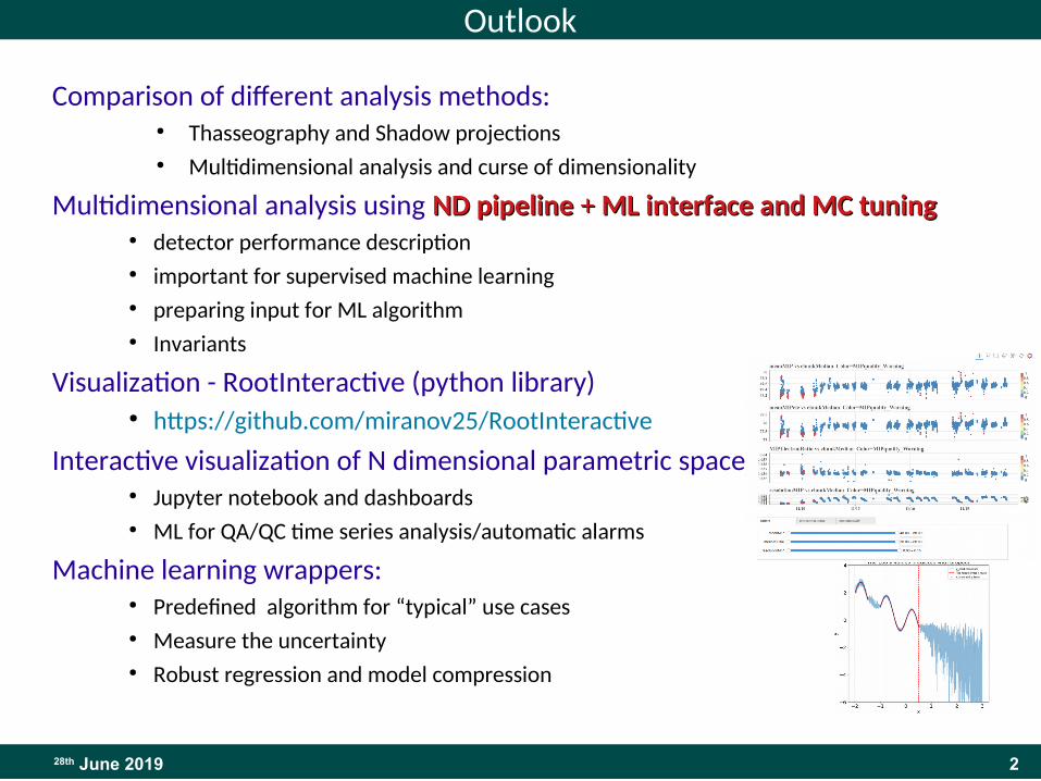
Outlook

Comparison of different analysis methods:● Thasseography and Shadow projections● Multidimensional analysis and curse of dimensionality

Multidimensional analysis using ND pipelineND pipeline + + ML interface and MC tuningML interface and MC tuning● detector performance description ● important for supervised machine learning● preparing input for ML algorithm ● Invariants

Visualization - RootInteractive (python library)● https://github.com/miranov25/RootInteractive

Interactive visualization of N dimensional parametric space● Jupyter notebook and dashboards ● ML for QA/QC time series analysis/automatic alarms

Machine learning wrappers:● Predefined algorithm for “typical” use cases● Measure the uncertainty● Robust regression and model compression

328th June 2018

RootInteractive demos

Code in github, pip, integrated into AliRoot, O2

RootInteractive tutorials:● Root like interface:

● tutorial/bokehDraw/bokehTreeDraw.ipynb

● New interface (since v0.0.9)● tutorial/bokehDraw/bokehDrawArray.ipynb

● Standalone application (dashboards e.g material for agenda or web page)● tutorial/bokehDraw/standAlone.ipynb

https://github.com/miranov25/RootInteractiveTest

Tutorial-demos using Alice data - performance maps visualization comparison● see full list in Index.ipynb notebook ● QA - JIRA/ADQT-3● dEdx pile-up - JIRA/ATO-465● dEdx parameterization + “spline” visualization - JIRA/ATO-485● Conversion maps data/MC - JIRA/PWGPP-527

Machine learning part including interactive histogram demo for next week.

428th June 2019

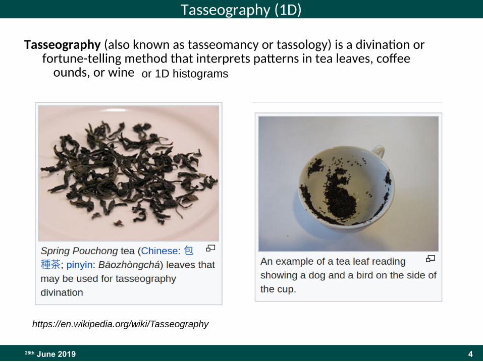
Tasseography (1D)

Tasseography (also known as tasseomancy or tassology) is a divination or fortune-telling method that interprets patterns in tea leaves, coffee grounds, or wine sediments.

https://en.wikipedia.org/wiki/Tasseography

or 1D histograms

528th June 2019

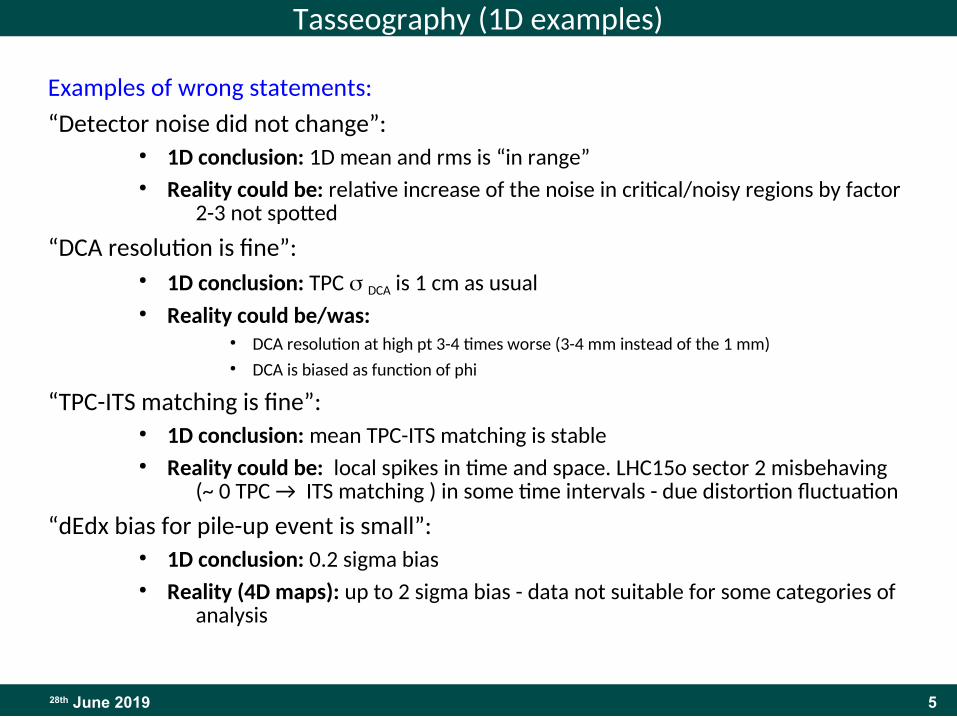
Tasseography (1D examples)

Examples of wrong statements:

“Detector noise did not change”:● 1D conclusion: 1D mean and rms is “in range” ● Reality could be: relative increase of the noise in critical/noisy regions by factor

2-3 not spotted

“DCA resolution is fine”:● 1D conclusion: TPC s DCA is 1 cm as usual● Reality could be/was:

● DCA resolution at high pt 3-4 times worse (3-4 mm instead of the 1 mm)● DCA is biased as function of phi

“TPC-ITS matching is fine”:● 1D conclusion: mean TPC-ITS matching is stable ● Reality could be: local spikes in time and space. LHC15o sector 2 misbehaving

(~ 0 TPC → ITS matching ) in some time intervals - due distortion fluctuation

“dEdx bias for pile-up event is small”:● 1D conclusion: 0.2 sigma bias● Reality (4D maps): up to 2 sigma bias - data not suitable for some categories of

analysis

628th June 2019

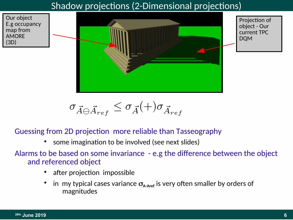
Shadow projections (2-Dimensional projections)

Guessing from 2D projection more reliable than Tasseography● some imagination to be involved (see next slides)

Alarms to be based on some invariance - e.g the difference between the object and referenced object

● after projection impossible● in my typical cases variance sA-Aref is very often smaller by orders of

magnitudes

Our objectE.g occupancy map from AMORE(3D)

Projection of object - Our current TPC DQM

728th June 2019

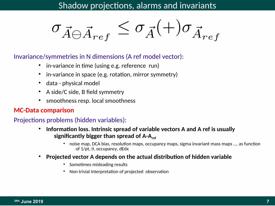
Shadow projections, alarms and invariants

Invariance/symmetries in N dimensions (A ref model vector):● in-variance in time (using e.g. reference run)● in-variance in space (e.g. rotation, mirror symmetry)● data - physical model● A side/C side, B field symmetry● smoothness resp. local smoothness

MC-Data comparison

Projections problems (hidden variables):● Information loss. Intrinsic spread of variable vectors A and A ref is usually

significantly bigger than spread of A-Aref

● noise map, DCA bias, resolution maps, occupancy maps, sigma invariant mass maps …. as function of 1/pt, q, occupancy, dEdx

● Projected vector A depends on the actual distribution of hidden variable● Sometimes misleading results● Non trivial interpretation of projected observation

828th June 2019

Example usage of N-Dimensional analysis pipeline in detector studies

● dEdx bias for pile-up events understood and partially mitigateddEdx bias for pile-up events understood and partially mitigated

928th June 2019

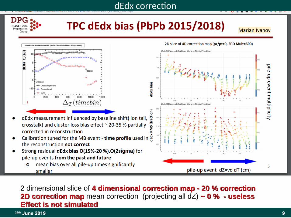
dEdx correction

2 dimensional slice of 4 dimensional correction map - 20 % correction4 dimensional correction map - 20 % correction2D correction map2D correction map mean correction (projecting all dZ) ~ 0 % - useless~ 0 % - uselessEffect is not simulatedEffect is not simulated

1028th June 2019

Multidimensional analysispipeline

● library (libStat) written in C++ (planned to be partially rewitten using optimized Python/C++ libraries)

● possible to use in Python● visualization written in Python - possible to invoke it in C++ (root)

1128th June 2018

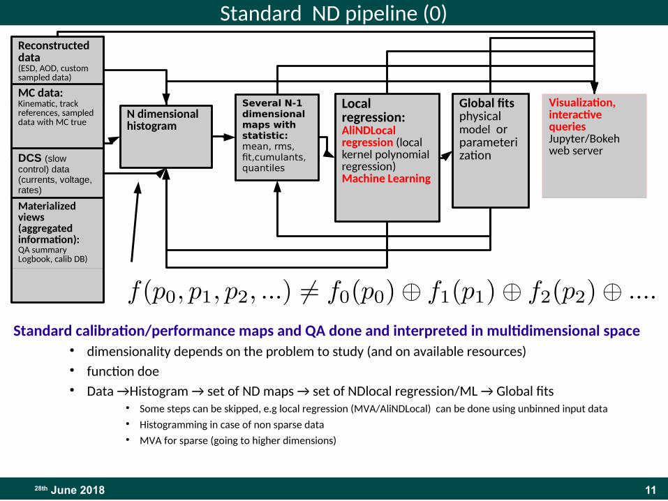
Standard ND pipeline (0)

Standard calibration/performance maps and QA done and interpreted in multidimensional space● dimensionality depends on the problem to study (and on available resources)● function doe● Data →Histogram → set of ND maps → set of NDlocal regression/ML → Global fits

● Some steps can be skipped, e.g local regression (MVA/AliNDLocal) can be done using unbinned input data● Histogramming in case of non sparse data ● MVA for sparse (going to higher dimensions)

Reconstructed data(ESD, AOD, custom sampled data)

Raw data

DCS (slow control) data(currents, voltage, rates)

N dimensional histogram

Several N-1 dimensional maps with statistic:mean, rms, fit,cumulants, quantiles

Local regression: AliNDLocal regression (local kernel polynomial regression)Machine Learning

Global fitsphysical model or parameterization

Visualization, interactive queries Jupyter/Bokeh web server

Materialized views (aggregated information):QA summaryLogbook, calib DB)

MC data:Kinematic, track references, sampled data with MC true

1228th June 2018

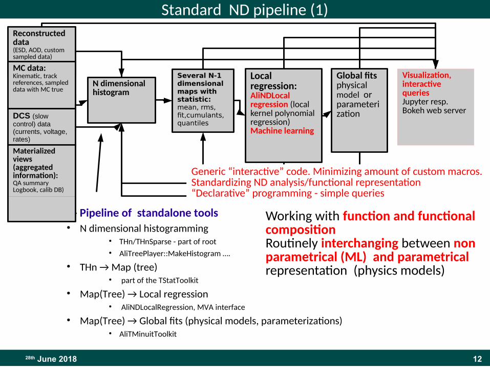
Standard ND pipeline (1)

libSTAT ()- Pipeline of standalone tools● N dimensional histogramming

● THn/THnSparse - part of root● AliTreePlayer::MakeHistogram ….

● THn → Map (tree)● part of the TStatToolkit

● Map(Tree) → Local regression● AliNDLocalRegression, MVA interface

● Map(Tree) → Global fits (physical models, parameterizations)● AliTMinuitToolkit

Working with function and functional compositionRoutinely interchanging between non parametrical (ML) and parametrical representation (physics models)

Reconstructed data(ESD, AOD, custom sampled data)

Raw data

DCS (slow control) data(currents, voltage, rates)

N dimensional histogram

Several N-1 dimensional maps with statistic:mean, rms, fit,cumulants, quantiles

Local regression: AliNDLocal regression (local kernel polynomial regression)Machine learning

Global fitsphysical model or parameterization

Visualization, interactive queries Jupyter resp. Bokeh web server

Materialized views (aggregated information):QA summaryLogbook, calib DB)

MC data:Kinematic, track references, sampled data with MC true

Generic “interactive” code. Minimizing amount of custom macros.Standardizing ND analysis/functional representation“Declarative” programming - simple queries

1328th June 2019

Curse of dimensionality. MVA/histogramming

When the dimensionality increases, the volume of the space increases so fast that the available data become sparse.

● The volume of a cube grows exponentially with increasing dimension

● The volume of a sphere grows exponentially with increasing dimension

● Most of the volume of a cube is very close to the (d − 1)-dimensional surface of the cube

https://en.wikipedia.org/wiki/Curse_of_dimensionality

Effect to be considered. Detector/reconstruction experts to be consulted ● Find relevant dimensions (2-6 dimensions)● Proper selection of variables (smooth or linear behavior)

● e.g q/pt instead of pt, occupancy/multiplicity instead of centrality● Proper binning. In case proper selection of variables, few bins needed

In the following examples I'm considering properly designed dimensionality/binning of the space

Other ML techniques in case of the sparse data (too high dimensions, time series)

1428th June 2019

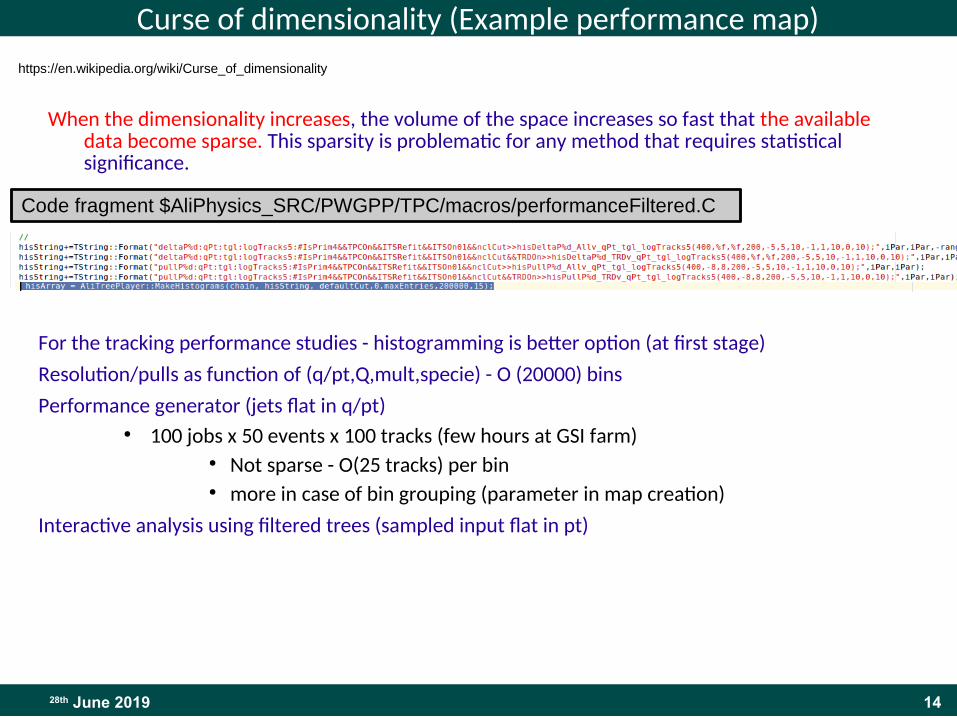
Curse of dimensionality (Example performance map)

When the dimensionality increases, the volume of the space increases so fast that the available data become sparse. This sparsity is problematic for any method that requires statistical significance.

For the tracking performance studies - histogramming is better option (at first stage)

Resolution/pulls as function of (q/pt,Q,mult,specie) - O (20000) bins

Performance generator (jets flat in q/pt)● 100 jobs x 50 events x 100 tracks (few hours at GSI farm)

● Not sparse - O(25 tracks) per bin● more in case of bin grouping (parameter in map creation)

Interactive analysis using filtered trees (sampled input flat in pt)

Code fragment $AliPhysics_SRC/PWGPP/TPC/macros/performanceFiltered.C

https://en.wikipedia.org/wiki/Curse_of_dimensionality

1528th June 2019

Usage of n-dimensional pipeline

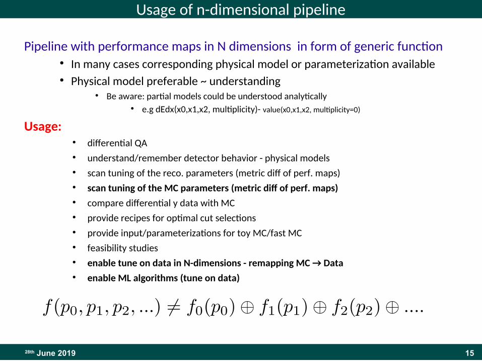
Pipeline with performance maps in N dimensions in form of generic function ● In many cases corresponding physical model or parameterization available● Physical model preferable ~ understanding

● Be aware: partial models could be understood analytically● e.g dEdx(x0,x1,x2, multiplicity)- value(x0,x1,x2, multiplicity=0)

Usage:● differential QA ● understand/remember detector behavior - physical models● scan tuning of the reco. parameters (metric diff of perf. maps)● scan tuning of the MC parameters (metric diff of perf. maps)● compare differential y data with MC● provide recipes for optimal cut selections● provide input/parameterizations for toy MC/fast MC● feasibility studies● enable tune on data in N-dimensions - remapping MC → Data ● enable ML algorithms (tune on data)

1628th June 2019

Example ND pipeline analysis

1728th June 2018

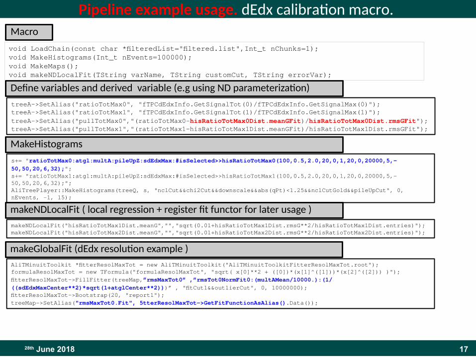
Pipeline example usage. dEdx calibration macro.

void LoadChain(const char *filteredList="filtered.list",Int_t nChunks=1);void MakeHistograms(Int_t nEvents=100000);void MakeMaps();void makeNDLocalFit(TString varName, TString customCut, TString errorVar);

treeA->SetAlias("ratioTotMax0", "fTPCdEdxInfo.GetSignalTot(0)/fTPCdEdxInfo.GetSignalMax(0)");treeA->SetAlias("ratioTotMax1", "fTPCdEdxInfo.GetSignalTot(1)/fTPCdEdxInfo.GetSignalMax(1)");treeA->SetAlias("pullTotMax0","(ratioTotMax0-hisRatioTotMax0Dist.meanGFit)/hisRatioTotMax0Dist.rmsGFit");treeA->SetAlias("pullTotMax1","(ratioTotMax1-hisRatioTotMax1Dist.meanGFit)/hisRatioTotMax1Dist.rmsGFit");

Macro

Define variables and derived variable (e.g using ND parameterization)

s+= "ratioTotMax0:atgl:multA:pileUpZ:sdEdxMax:#isSelected>>hisRatioTotMax0(100,0.5,2.0,20,0,1,20,0,20000,5,-50,50,20,6,32);";s+= "ratioTotMax1:atgl:multA:pileUpZ:sdEdxMax:#isSelected>>hisRatioTotMax1(100,0.5,2.0,20,0,1,20,0,20000,5,-50,50,20,6,32);";AliTreePlayer::MakeHistograms(treeQ, s, "nclCut&&chi2Cut&&downscale&&abs(qPt)<1.25&&nclCutGold&&pileUpCut", 0, nEvents, -1, 15);

MakeHistograms

makeNDLocalFit("hisRatioTotMax1Dist.meanG","","sqrt(0.01+hisRatioTotMax1Dist.rmsG**2/hisRatioTotMax1Dist.entries)"); makeNDLocalFit("hisRatioTotMax2Dist.meanG","","sqrt(0.01+hisRatioTotMax2Dist.rmsG**2/hisRatioTotMax2Dist.entries)");

makeNDLocalFit ( local regression + register fit functor for later usage )

AliTMinuitToolkit *fitterResolMaxTot = new AliTMinuitToolkit("AliTMinuitToolkitFitterResolMaxTot.root");formulaResolMaxTot = new TFormula("formulaResolMaxTot", "sqrt( x[0]**2 + ([0])*(x[1]^([1]))*(x[2]^([2])) )");fitterResolMaxTot->FillFitter(treeMap,”rmsMaxTot0” ,”rmsTot0NormFit0:(multAMean/10000.):(1/((sdEdxMaxCenter**2)*sqrt(1+atglCenter**2)))” , "fitCut1&&outlierCut", 0, 10000000);fitterResolMaxTot->Bootstrap(20, "report1");treeMap->SetAlias("rmsMaxTot0.Fit", fitterResolMaxTot->GetFitFunctionAsAlias().Data());

makeGlobalFit (dEdx resolution example )

1828th June 2018

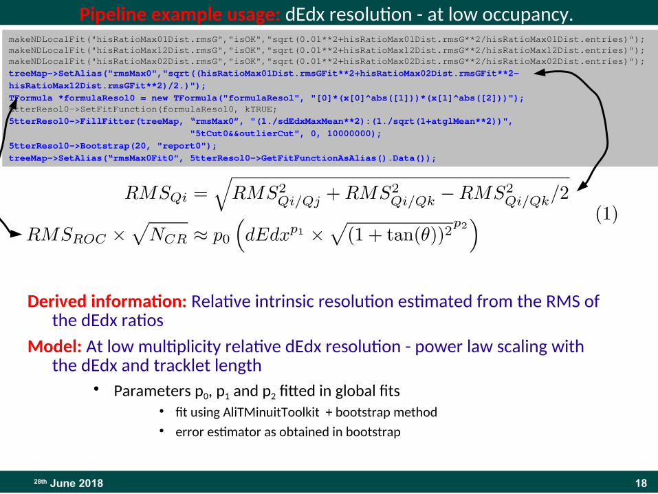
Pipeline example usage: dEdx resolution - at low occupancy.

Derived information: Relative intrinsic resolution estimated from the RMS of the dEdx ratios

Model: At low multiplicity relative dEdx resolution - power law scaling with the dEdx and tracklet length

● Parameters p0, p1 and p2 fitted in global fits● fit using AliTMinuitToolkit + bootstrap method● error estimator as obtained in bootstrap

makeNDLocalFit("hisRatioMax01Dist.rmsG","isOK","sqrt(0.01**2+hisRatioMax01Dist.rmsG**2/hisRatioMax01Dist.entries)"); makeNDLocalFit("hisRatioMax12Dist.rmsG","isOK","sqrt(0.01**2+hisRatioMax12Dist.rmsG**2/hisRatioMax12Dist.entries)"); makeNDLocalFit("hisRatioMax02Dist.rmsG","isOK","sqrt(0.01**2+hisRatioMax02Dist.rmsG**2/hisRatioMax02Dist.entries)");treeMap->SetAlias("rmsMax0","sqrt((hisRatioMax01Dist.rmsGFit**2+hisRatioMax02Dist.rmsGFit**2-hisRatioMax12Dist.rmsGFit**2)/2.)");TFormula *formulaResol0 = new TFormula("formulaResol", "[0]*(x[0]^abs([1]))*(x[1]^abs([2]))");fitterResol0->SetFitFunction(formulaResol0, kTRUE;fitterResol0->FillFitter(treeMap, “rmsMax0”, "(1./sdEdxMaxMean**2):(1./sqrt(1+atglMean**2))", "fitCut0&&outlierCut", 0, 10000000);fitterResol0->Bootstrap(20, "report0");treeMap->SetAlias(“rmsMax0Fit0", fitterResol0->GetFitFunctionAsAlias().Data());

1928th June 2018

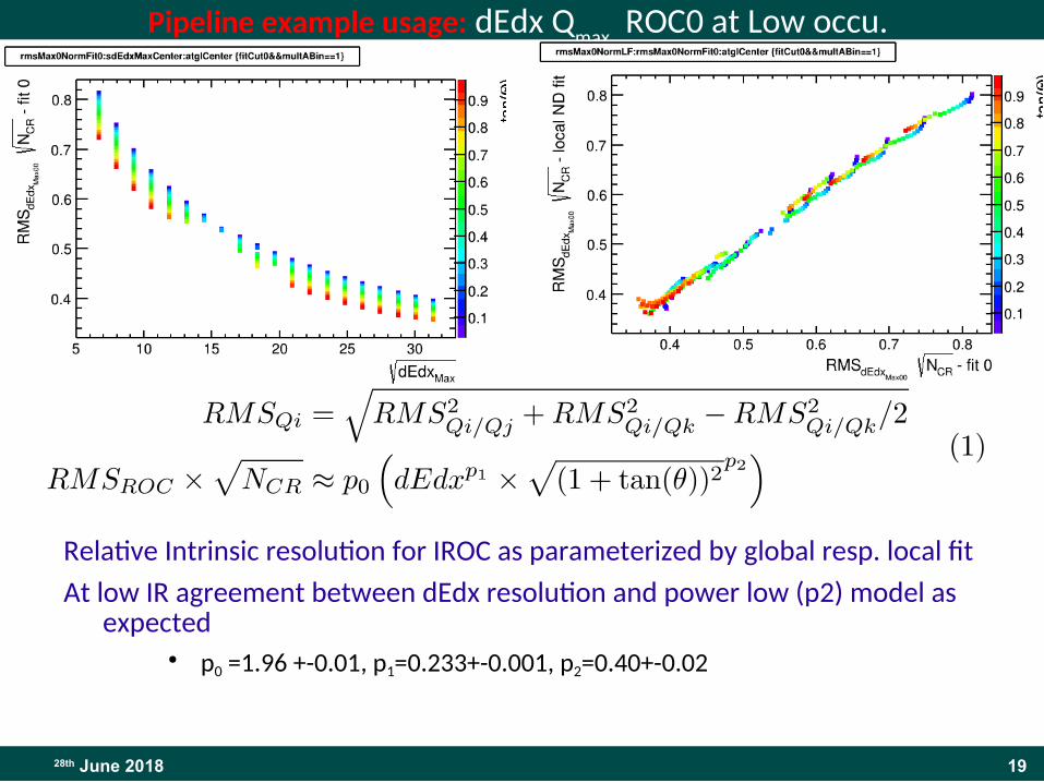
Pipeline example usage: dEdx Qmax

ROC0 at Low occu.

Relative Intrinsic resolution for IROC as parameterized by global resp. local fit

At low IR agreement between dEdx resolution and power low (p2) model as expected

● p0 =1.96 +-0.01, p1=0.233+-0.001, p2=0.40+-0.02

2028th June 2018

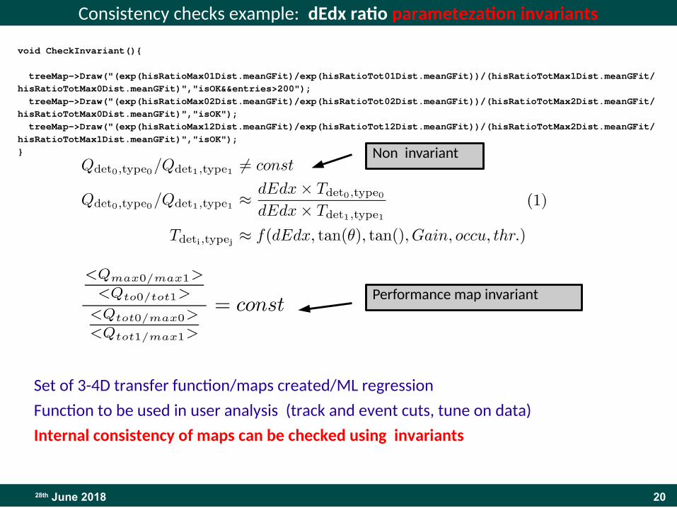
Consistency checks example: dEdx ratio parametezation invariants

Set of 3-4D transfer function/maps created/ML regression

Function to be used in user analysis (track and event cuts, tune on data)

Internal consistency of maps can be checked using invariants

void CheckInvariant(){

treeMap->Draw("(exp(hisRatioMax01Dist.meanGFit)/exp(hisRatioTot01Dist.meanGFit))/(hisRatioTotMax1Dist.meanGFit/hisRatioTotMax0Dist.meanGFit)","isOK&&entries>200"); treeMap->Draw("(exp(hisRatioMax02Dist.meanGFit)/exp(hisRatioTot02Dist.meanGFit))/(hisRatioTotMax2Dist.meanGFit/hisRatioTotMax0Dist.meanGFit)","isOK"); treeMap->Draw("(exp(hisRatioMax12Dist.meanGFit)/exp(hisRatioTot12Dist.meanGFit))/(hisRatioTotMax2Dist.meanGFit/hisRatioTotMax1Dist.meanGFit)","isOK");}

Performance map invariant

Non invariant

2128th June 2018

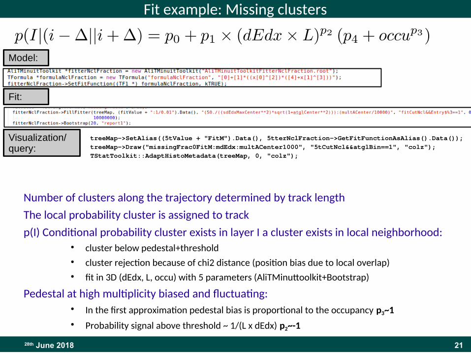
Fit example: Missing clusters

Number of clusters along the trajectory determined by track length

The local probability cluster is assigned to track

p(I) Conditional probability cluster exists in layer I a cluster exists in local neighborhood: ● cluster below pedestal+threshold● cluster rejection because of chi2 distance (position bias due to local overlap)● fit in 3D (dEdx, L, occu) with 5 parameters (AliTMinuttoolkit+Bootstrap)

Pedestal at high multiplicity biased and fluctuating:● In the first approximation pedestal bias is proportional to the occupancy p3~1

● Probability signal above threshold ~ 1/(L x dEdx) p2~-1

Model:

Fit:

Visualization/query:

treeMap->SetAlias((fitValue + "FitM").Data(), fitterNclFraction->GetFitFunctionAsAlias().Data());treeMap->Draw("missingFrac0FitM:mdEdx:multACenter1000", "fitCutNcl&&atglBin==1", "colz");TStatToolkit::AdaptHistoMetadata(treeMap, 0, "colz");

2228th June 2018

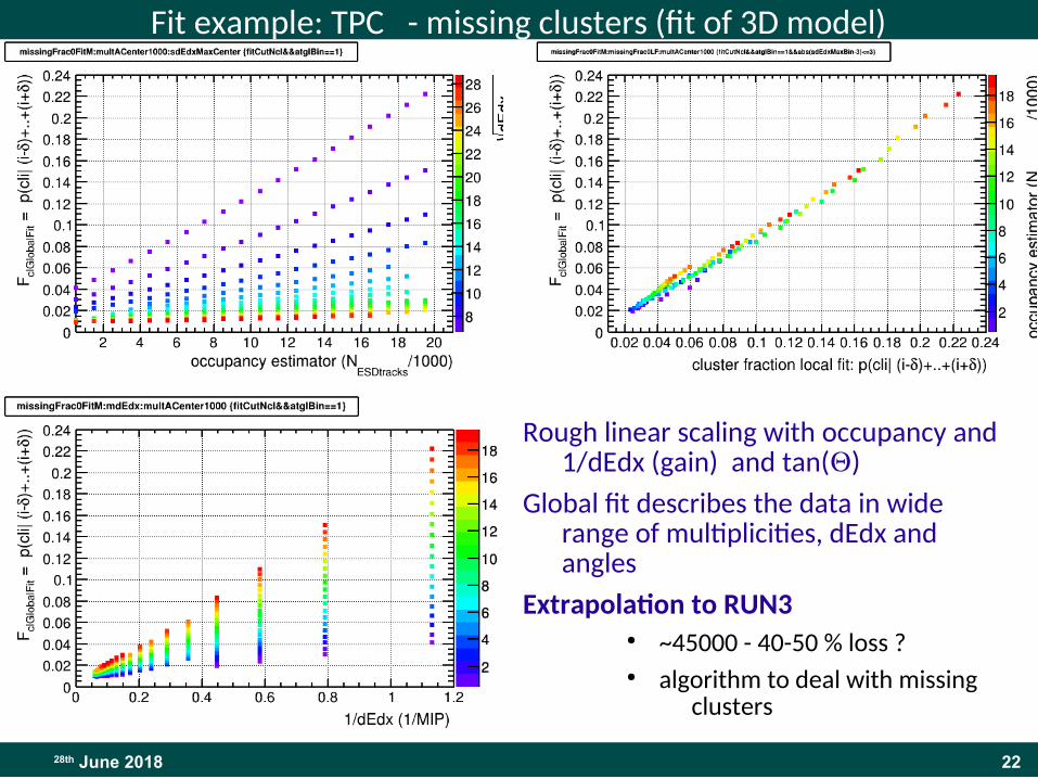
Fit example: TPC - missing clusters (fit of 3D model)

Rough linear scaling with occupancy and 1/dEdx (gain) and tan(Q)

Global fit describes the data in wide range of multiplicities, dEdx and angles

Extrapolation to RUN3● ~45000 - 40-50 % loss ?● algorithm to deal with missing

clusters

2328th June 2018

MC parameters tuningOptions:

● tune parameters of MC (sometimes slow algorithm to be involved)● tune MC performance

2428th June 2018

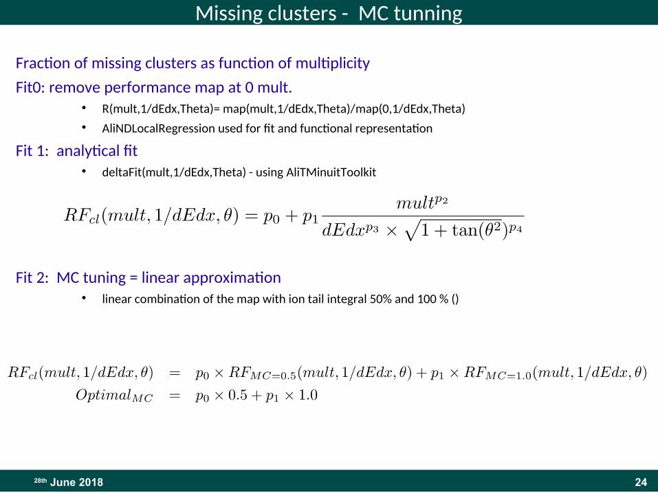
Missing clusters - MC tunning

Fraction of missing clusters as function of multiplicity

Fit0: remove performance map at 0 mult.● R(mult,1/dEdx,Theta)= map(mult,1/dEdx,Theta)/map(0,1/dEdx,Theta)● AliNDLocalRegression used for fit and functional representation

Fit 1: analytical fit● deltaFit(mult,1/dEdx,Theta) - using AliTMinuitToolkit

Fit 2: MC tuning = linear approximation● linear combination of the map with ion tail integral 50% and 100 % ()

2528th June 2018

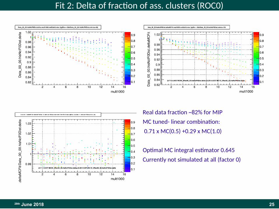
Fit 2: Delta of fraction of ass. clusters (ROC0)

Real data fraction ~82% for MIP

MC tuned- linear combination:

0.71 x MC(0.5) +0.29 x MC(1.0)

Optimal MC integral estimator 0.645

Currently not simulated at all (factor 0)

2628th June 2019

RootInteractive

2728th June 2019

Inroduction:

Introduction:

During the ROOT workshop I presented Alice N-Dimensional analysis pipeline. After the presentation I was contacted by one of author of JUPYTER package Sylvain Corlay. He proposed to use Jupyter for interactive visualization of n-dimensional data.

As a follow up of discussion with Sylvain Corlay during the ROOT workshop.

I started to work on RootInteractive tool.

2828th June 2019

RootInteractive

Why RootInteractive?● RootInteractive is an Python 2 and (soon 3) library for data analysis and visualization. Python already has

excellent tools like numpy, pandas, and xarray for data processing, and bokeh and matplotlib for plotting, so why yet another library?

RootInteractive helps you understand your data better, by letting you work seamlessly with both the data and its graphical representation.

RootInteractive focuses on bundling your data together with the appropriate metadata to support both analysis and visualization, making your raw data and its visualization equally accessible at all times.

With RootInteractive, instead of building a plot using direct calls to a plotting library, you first describe your data with a small amount of crucial semantic information required to make it visualizable, then you specify additional metadata as needed to determine more detailed aspects of your visualization. This approach provides immediate, automatic visualization that can be effortlessly requested at any time as your data evolves, rendered automatically by one of the supported plotting libraries (such as Bokeh or Matplotlib).

Inspired by the HoloViews project + support for the Root/AliRoot ● possibility to use the code in C++ → in case function to be used in root/C++ parameters by string ● string parsed to python structures internally

2928th June 2018

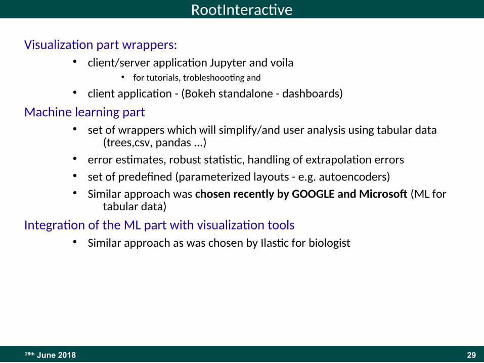
RootInteractive

Visualization part wrappers:● client/server application Jupyter and voila

● for tutorials, trobleshoooting and

● client application - (Bokeh standalone - dashboards)

Machine learning part● set of wrappers which will simplify/and user analysis using tabular data

(trees,csv, pandas ...)● error estimates, robust statistic, handling of extrapolation errors● set of predefined (parameterized layouts - e.g. autoencoders)● Similar approach was chosen recently by GOOGLE and Microsoft (ML for

tabular data)

Integration of the ML part with visualization tools● Similar approach as was chosen by Ilastic for biologist

3028th June 2019

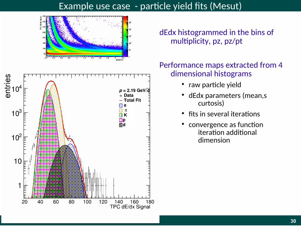
Example use case - particle yield fits (Mesut)

dEdx histogrammed in the bins of multiplicity, pz, pz/pt

Performance maps extracted from 4 dimensional histograms

● raw particle yield● dEdx parameters (mean,s

curtosis)● fits in several iterations● convergence as function

iteration additional dimension

3128th June 2019

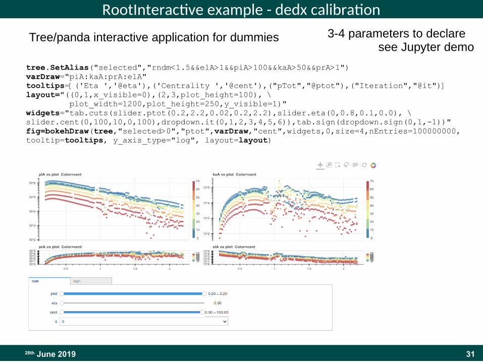
RootInteractive example - dedx calibration

tree.SetAlias("selected","rndm<1.5&&elA>1&&piA>100&&kaA>50&&prA>1")varDrawvarDraw="piA:kaA:prA:elA"tooltips=[('Eta ','@eta'),('Centrality ','@cent'),("pTot","@ptot"),("Iteration","@it")]layout="((0,1,x_visible=0),(2,3,plot_height=100), \ plot_width=1200,plot_height=250,y_visible=1)"widgets="tab.cuts(slider.ptot(0.2,2.2,0.02,0.2,2.2),slider.eta(0,0.8,0.1,0.0), \ slider.cent(0,100,10,0,100),dropdown.it(0,1,2,3,4,5,6)),tab.sign(dropdown.sign(0,1,-1))"fig=bokehDraw(tree,"selected>0","ptot",varDraw,"cent",widgets,0,size=4,nEntries=100000000,tooltip=tooltips, y_axis_type="log", layout=layout)

Tree/panda interactive application for dummies 3-4 parameters to declare see Jupyter demo

3230th November 2018

33

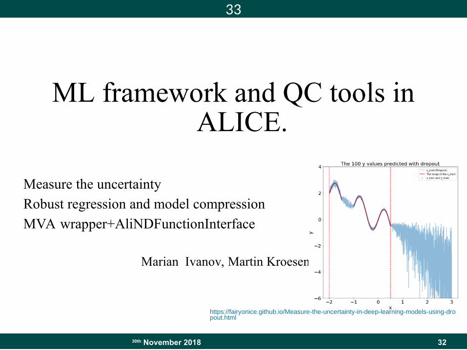
ML framework and QC tools in ALICE.

Measure the uncertainty

Robust regression and model compression

MVA wrapper+AliNDFunctionInterface

Marian Ivanov, Martin Kroesen

https://fairyonice.github.io/Measure-the-uncertainty-in-deep-learning-models-using-dropout.html

3330th November 2018

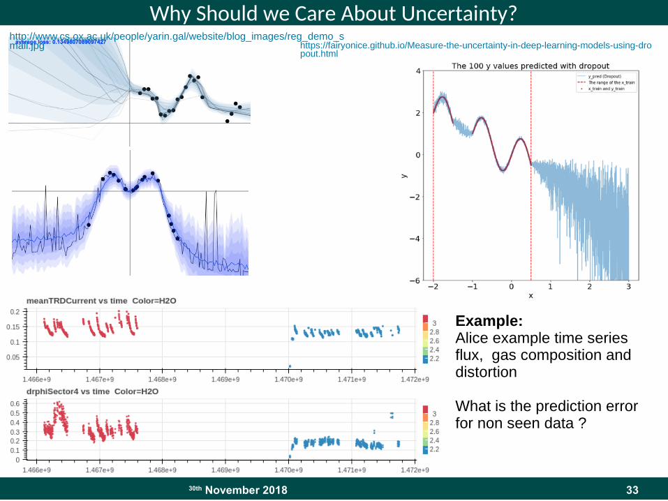
Why Should we Care About Uncertainty?

https://fairyonice.github.io/Measure-the-uncertainty-in-deep-learning-models-using-dropout.html

http://www.cs.ox.ac.uk/people/yarin.gal/website/blog_images/reg_demo_small.jpg

Example:Alice example time seriesflux, gas composition and distortion

What is the prediction errorfor non seen data ?

3430th November 2018

Confidence/prediction intervals

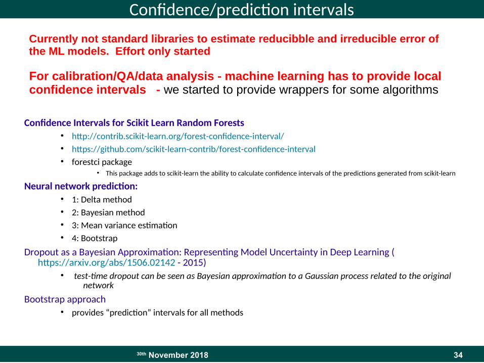
Confidence Intervals for Scikit Learn Random Forests● http://contrib.scikit-learn.org/forest-confidence-interval/● https://github.com/scikit-learn-contrib/forest-confidence-interval● forestci package

● This package adds to scikit-learn the ability to calculate confidence intervals of the predictions generated from scikit-learn

Neural network prediction:● 1: Delta method● 2: Bayesian method● 3: Mean variance estimation● 4: Bootstrap

Dropout as a Bayesian Approximation: Representing Model Uncertainty in Deep Learning (https://arxiv.org/abs/1506.02142 - 2015)

● test-time dropout can be seen as Bayesian approximation to a Gaussian process related to the original network

Bootstrap approach● provides “prediction” intervals for all methods

Currently not standard libraries to estimate reducibble and irreducible error of the ML models. Effort only started

For calibration/QA/data analysis - machine learning has to provide local confidence intervals - we started to provide wrappers for some algorithms

3528th June 2019

Time interval QA + time seriesRun2 example of investigation/problems

3628th June 2018

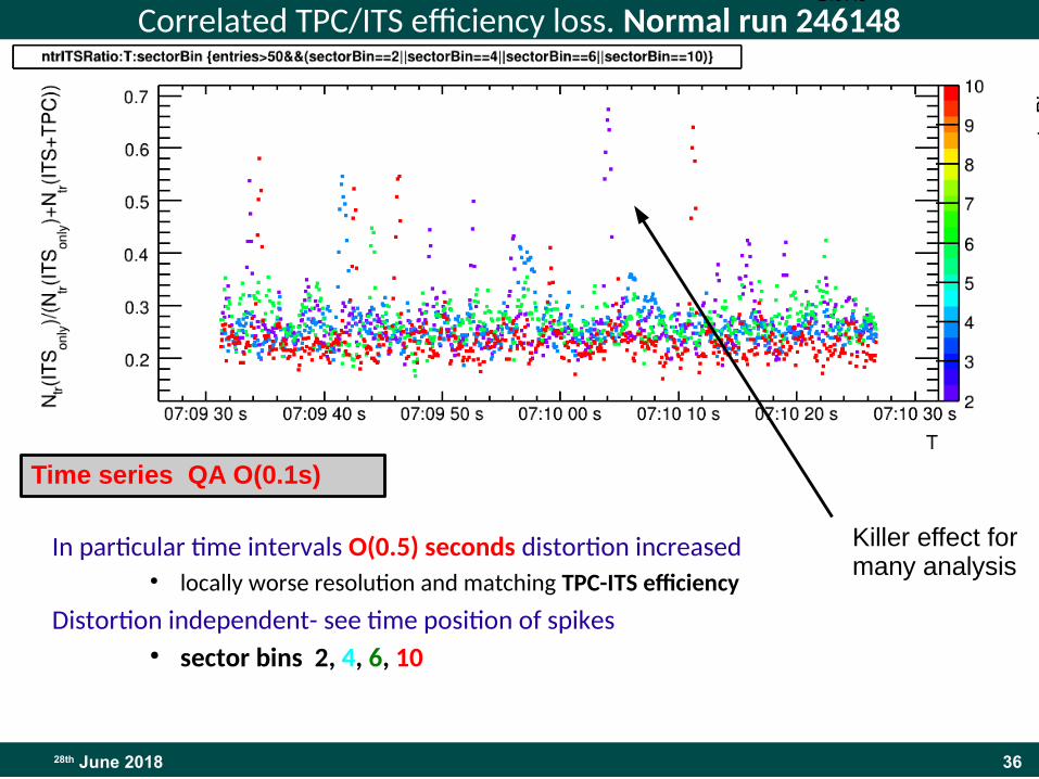
Correlated TPC/ITS efficiency loss. Normal run 246148

In particular time intervals O(0.5) seconds distortion increased● locally worse resolution and matching TPC-ITS efficiency

Distortion independent- see time position of spikes ● sector bins 2, 4, 6, 10

246148

●

●

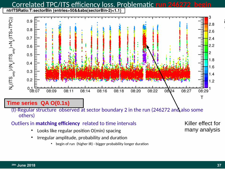
Time series QA O(0.1s)

Killer effect for many analysis

3728th June 2018

Correlated TPC/ITS efficiency loss. Problematic run 246272 begin

(I)-Regular structure observed at sector boundary 2 in the run (246272 and also some others)

Outliers in matching efficiency related to time intervals● Looks like regular position O(min) spacing● Irregular amplitude, probability and duration

● begin of run (higher IR) - bigger probability longer duration

246148

Time series QA O(0.1s)

Killer effect for many analysis

3828th June 2019

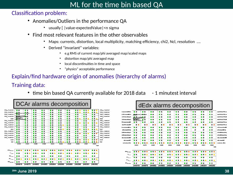
ML for the time bin based QAClassification problem:

● Anomalies/Outliers in the performance QA● usually [ |value-expectedValue|<n sigma

● Find most relevant features in the other observables● Maps: currents, distortion, local multiplicity, matching efficiency, chi2, Ncl, resolution ….● Derived “invariant” variables:

● e.g RMS of current map/phi averaged map/scaled maps● distortion map/phi averaged map● local discontinuities in time and space● “physics” acceptable performance

Explain/find hardware origin of anomalies (hierarchy of alarms)

Training data:● time bin based QA currently available for 2018 data - 1 minutest interval

dEdx alarms decompositionDCAr alarms decomposition

3928th June 2019

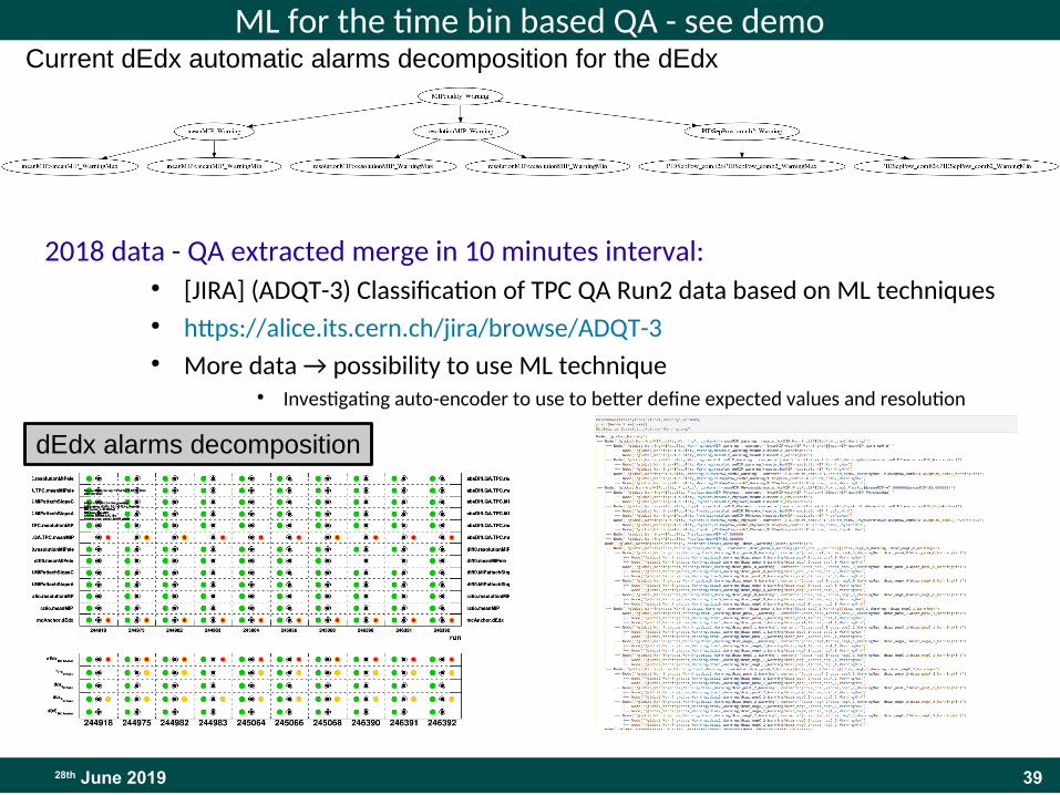
ML for the time bin based QA - see demo

2018 data - QA extracted merge in 10 minutes interval:● [JIRA] (ADQT-3) Classification of TPC QA Run2 data based on ML techniques● https://alice.its.cern.ch/jira/browse/ADQT-3● More data → possibility to use ML technique

● Investigating auto-encoder to use to better define expected values and resolution

dEdx alarms decomposition

Current dEdx automatic alarms decomposition for the dEdx

4028th June 2018

RootInteractive - short summary

Visualization part wrappers:● client/server application (Jupyter+Bokeh+???)● client application - (Bokeh standalone - dashboards)

Machine learning part, as I presented in December ML workshop● set of wrappers which will simplify/and user analysis using tabular data (trees,csv,

pandas ...)● error estimates, robust statistic, handling of extrapolation errors● set of predefined (parameterized layouts - e.g. autoencoders)● Similar approach was chosen recently by GOOGLE and Microsoft (ML for tabular data)

Integration of the ML part with visualization tools● Similar approach as was chosen by Ilastic project for biologist

Usage:● calibration● reconstruction performance tuning● Physics (interactive) analysis● QA/QC ● ….

4128th June 2018

Google announcement

●GOOGLE - 3 weeks ago (sent to QA/QC)● https://news.ycombinator.com/item?id=19626275● https://techcrunch.com/2019/04/10/google-expands-its-ai-services/

As expected, Google used the second day of its annual Cloud Next conference to shine a spotlight on its AI tools. The company made a dizzying number of announcements today, but at the core of all of these new tools and services is the company’s plan to democratize the company’s plan to democratize AI and machine learning with pre-built modelsAI and machine learning with pre-built models and easier to use services, while also giving more advanced developers the tools to build their own custom models.

The highlight of today’s announcements is the beta launch of the company’s AI Platform. The idea here is to offer developers and data scientists an end-to-end service for building, testing and deploying their own models. To do this, the service brings together a variety of existing and new products that allow you to build a full data pipeline to pull in data, label it (with the help of a new built-in labeling service) and then either use existing classification, object recognition or entity extraction models, or use existing tools like AutoML or the Cloud Machine Learning engine to train and deploy custom models. ...

One of these new features is AutoML Tables,AutoML Tables, which takes existing tabular data that may sit in Google’s BigQuery database or in a storage service and automatically creates a model that automatically creates a model that will predict the value of a given columnwill predict the value of a given column..

4228th June 2018

Microsoft announcment

Source:● https://techcrunch.com/2019/05/02/microsoft-makes-a-push-to-simplify-machine-learning/

Ahead of its Build conference, Microsoft today released a slew of new machine learning products and tweaks to some of its existing services. These range from no-code tools to hosted notebooks, with a number of new APIs and other services in-between. The core theme, here, though, is that Microsoft iMicrosoft is continuing its strategy of democratizing access to s continuing its strategy of democratizing access to AI.AI.

Ahead of the release, I sat down with Microsoft’s Eric Boyd, the company’s corporate vice president of its AI platform, to discuss Microsoft’s take on this space, where it competes heavily with the likes of Google and AWS, as well as numerous, often more specialized startups. And to some degree, the actual machine learning technologies have become table stakes. Everybody now offers pre-trained models, open-source tools and the platforms to Everybody now offers pre-trained models, open-source tools and the platforms to train, build and deploy models. If one company doesn’t have pre-trained models for some train, build and deploy models. If one company doesn’t have pre-trained models for some use cases that its competitors support, it’s only a matter of time before it will.use cases that its competitors support, it’s only a matter of time before it will. It’s the auxiliary services and the overall developer experience, though, where companies like Microsoft, with its long history of developing these tools, can differentiate themselves. ...