EU

GS

*‡V

nftacaibsbdsIadsaobso©

mbi

C6

METHODS 19, 253–269 (1999)

A

1CA

xploring Biomolecular Recognitionsing Optical Biosensors

abriela Canziani,* Wentao Zhang,* Douglas Cines,† Ann Rux,‡haron Willis,‡ Gary Cohen,‡ Roselyn Eisenberg,§ and Irwin Chaiken*,1

rticle ID meth.1999.0855, available online at http://www.idealibrary.com on

Department of Medicine and †Department of Pathology and Laboratory Medicine, School of Medicine;Department of Microbiology, School of Dental Medicine; and §Department of Pathobiology, School ofeterinary Medicine, University of Pennsylvania, Philadelphia, Pennsylvania 19104

tbnticqratrmrmtsirfifii

ttcmsaost

Understanding the basic forces that determine molecular recog-ition helps to elucidate mechanisms of biological processes andacilitates discovery of innovative biotechnological methods and ma-erials for therapeutics, diagnostics, and separation science. Thebility to measure interaction properties of biological macromole-ules quantitatively across a wide range of affinity, size, and purity is

growing need of studies aimed at characterizing biomolecularnteractions and the structural elements that drive them. Opticaliosensors have provided an increasingly impactful technology foruch biomolecular interaction analyses. These biosensors record theinding and dissociation of macromolecules in real time by trans-ucing the accumulation of mass of an analyte molecule at theensor surface coated with ligand molecule into an optical signal.nteractions of analytes and ligands can be analyzed at a microscalend without the need to label either interactant. Sensors enable theetection of bimolecular interaction as well as multimolecular as-embly. Most notably, the method is quantitative and kinetic, en-bling determination of both steady-state and dynamic parametersf interaction. This article describes the basic methodology of opticaliosensors and presents several examples of its use to investigateuch biomolecular systems as cytokine growth factor–receptor rec-gnition, coagulation factor assembly, and virus–cell docking.1999 Academic Press

Specific molecular interactions provide the funda-ental mechanism for selectivity in every aspect of

iological structure and function. Hence, understand-ng the basic forces that determine molecular recogni-

se

1 To whom correspondence should be addressed at 913 Stellarhance Laboratories, 422 Curie Boulevard, Philadelphia, PA 19104–100. E-mail: chaiken@mail.med.upenn.edu. Fax: (215) 349–5572.

046-2023/99 $30.00opyright © 1999 by Academic Pressll rights of reproduction in any form reserved.

ion helps to elucidate the mechanisms of importantiological processes and facilitates the discovery of in-ovative biotechnological methods and materials forherapeutics, diagnostics, and separation science. Rap-dly expanding identification of biological macromole-ules, in particular proteins, through mass gene se-uencing and increasing availability of their atomicesolution three-dimensional structures from NMRnd crystallography provide important starting pointso investigate those parts of these molecules that driveecognition mechanisms. Furthermore, the advent ofethodologies to modify structure, in particular using

ecombinant-based protein mutagenesis and design,akes it possible to identify structural elements in

hese folded molecules that are key determinants ofpecificity and affinity. Against this backdrop, the abil-ty to measure interaction properties of biological mac-omolecules quantitatively across a wide range of af-nity, size, and purity is a growing need of structure–unction studies. Optical biosensors have provided anncreasingly impactful technology for macromolecularnteraction analysis.

Optical biosensors record the binding and dissocia-ion of macromolecules in real time, therein offeringhe opportunity to measure both equilibrium affinityonstants and the on and off rate constants for macro-olecular interactions. The underlying principle of bio-

ensors, developed earlier with such techniques as an-lytical affinity chromatography, is twofold: (i) the usef a ligand immobilized on a solid phase as an affinityurface to bind one or more soluble analytes; and (ii)he measurement of mass migration on the affinity

urface to quantitate the analyte’s ligand binding prop-rties. Biosensors do this by optically detecting mass

253

bi

pmttvlrtawisspebcimctTlslbsm

sap

I

ttpaftc(Iatcltrifcmslv

Fueot

254 CANZIANI ET AL.

uildup on a sensor surface when the analyte binds tommobilized ligand.

The advantages of biosensor analysis over other ap-roaches are severalfold. (i) First, since the monochro-atic light-based optical detection of mass is essen-

ially immediate, biosensors enable the binding evento be visualized in real time. In turn, real-time obser-ation of binding enables kinetic analysis of macromo-ecular interactions, thus providing information aboutates of binding reactions that are unavailable withechniques that measure only binding equilibria, suchs titration calorimetry. Hence, optical biosensorsiden the window of investigation of biomolecules to

nclude not only equilibrium measurements at steadytate but also interaction dynamics. (ii) Second, biosen-ors facilitate measurement of interaction properties ofrotein variants produced by recombinant DNA, hencexpanding the ability to map recognition epitopes andinding surfaces. Biosensor features that facilitate re-ombinant variant analysis include no need for labelednteractants; a sensitivity at microscale; and anchoring

ethods that enable affinity purification of the ligandomponent on the sensor surface and hence can bypasshe need for complete prepurification of ligands. (iii)hird, interactions of analytes to preexisting noncova-

ent (but necessarily stable) complexes on the sensorurface can be monitored, hence allowing multimolecu-ar complexes and the dynamics of such complexes toe detected. (iv) Since the equilibrium affinity con-tants of two ligands for a receptor or other biologicalacromolecule can be the same while their rate con-

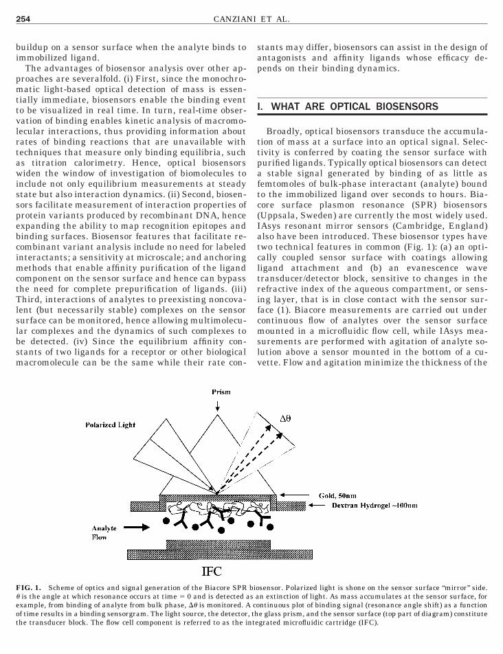
IG. 1. Scheme of optics and signal generation of the Biacore SPRis the angle at which resonance occurs at time 5 0 and is detected a

xample, from binding of analyte from bulk phase, Du is monitored. A cof time results in a binding sensorgram. The light source, the detector, thhe transducer block. The flow cell component is referred to as the inte

tants may differ, biosensors can assist in the design ofntagonists and affinity ligands whose efficacy de-ends on their binding dynamics.

. WHAT ARE OPTICAL BIOSENSORS

Broadly, optical biosensors transduce the accumula-ion of mass at a surface into an optical signal. Selec-ivity is conferred by coating the sensor surface withurified ligands. Typically optical biosensors can detectstable signal generated by binding of as little as

emtomoles of bulk-phase interactant (analyte) boundo the immobilized ligand over seconds to hours. Bia-ore surface plasmon resonance (SPR) biosensorsUppsala, Sweden) are currently the most widely used.Asys resonant mirror sensors (Cambridge, England)lso have been introduced. These biosensor types havewo technical features in common (Fig. 1): (a) an opti-ally coupled sensor surface with coatings allowingigand attachment and (b) an evanescence waveransducer/detector block, sensitive to changes in theefractive index of the aqueous compartment, or sens-ng layer, that is in close contact with the sensor sur-ace (1). Biacore measurements are carried out underontinuous flow of analytes over the sensor surfaceounted in a microfluidic flow cell, while IAsys mea-

urements are performed with agitation of analyte so-ution above a sensor mounted in the bottom of a cu-ette. Flow and agitation minimize the thickness of the

sensor. Polarized light is shone on the sensor surface “mirror” side.n extinction of light. As mass accumulates at the sensor surface, for

bios a

ntinuous plot of binding signal (resonance angle shift) as a functione glass prism, and the sensor surface (top part of diagram) constitutegrated microfluidic cartridge (IFC).

dts

O

lloiatmidamcg0t1bDh1

S

cmacgo((tiecvonafbantt

S

d

iltamssob(td

rartmgdmf

I

mmi

Fo

255BIOMOLECULAR RECOGNITION USING OPTICAL BIOSENSORS

iffusion layer and hence maximize the contact be-ween analyte and immobilized ligand at the sensorurface.

ptics

Detection of binding and dissociation events thatead to increase and decrease, respectively, of molecu-ar mass at the sensor surface is the direct consequencef refractive index change at the sensor/bulk phasenterface. In SPR, increase in refractive index leads toltered refraction of incident polarized light and, inurn, increase in angle of absorbance maxima by plas-on electrons of the gold film of the sensor at the water

nterface (1–3). Hence, the shift in angle can be relatedirectly to the concentration of solute and mass boundt the surface layer (4). The excitation of surface plas-on electrons is referred to as resonance. The pro-

essed resonance signal, referred to as response (R), isiven in resonance units (RU) and has a resolution of.001° Du, which is equivalent to 1025 change in refrac-ive index in the range 1.33–1.40, or a mass change of0 pg/mm2 (5). The high signal-to-noise ratio achievedy SPR permits binding of molecules as small as 200a to be detected using the Biacore. Kinetic modelsave been applied successfully to molecules as small as500 Da (6).

pecificity

Selectivity is conferred to an optical biosensor byoating the sensor surface with a specific ligand. Theost commonly used methods to immobilize ligands

re (i) direct covalent coupling and (ii) noncovalentapture by a covalently immobilized anchor. A majoroal in immobilization is to ensure a stable attachmentf ligand to sensor surface without ligand inactivation7). The SPR sensor surface consists of a thioalkane16-carbon chain) linker layer, attached to a gold layer,o which a noncrosslinked carboxylated dextran matrixs bound. The dextran matrix provides a hydrophilicnvironment for molecular interactions, facilitates theovalent coupling of ligands via specific carboxyl deri-atization, and reduces nonspecific absorption of bi-molecules to the otherwise flat sensor surface (8). Theoncrosslinked nature of the Biacore dextran matrixllows both ligand immobilization with minimal con-ormational distortion and maximum access of theinding epitopes of ligand and analyte. The addition ofhydrogel matrix attached to the surface optimizes theumber and accessibility of binding sites. It has ahickness approximately equal to the distance at whichhe evanescence field is 1/e of its strength.

ensitivity

The sensitivity of an optical biosensor instrumentepends on two main factors: the capacity of the sens-

raf

ng layer to bind the analyte and the optical detectionimit. The first depends on the affinity of the interac-ion and the number of binding sites accessible to thenalyte. The second factor controlling sensitivity, theinimum amount of bound analyte that can generate a

ignal, depends on the molecular mass of the analyte,ignal-to-noise ratio, and baseline drift (9). In the casef the SPR detector, for example, the minimum reliableinding signal for myoglobin (17 kDa) to a specific MAb109 M21 K a) is obtained at 1 pM. The sensitivity forhe binding interaction is reduced as a function of theistance of the ligand from the sensor surface (4).Overall, optical biosensors measure changes in the

efractive index profile across a solid/liquid interface asfunction of time, at constant temperature. Events

elated to the generation of resonance, integration ofhe transducer, detection of the optical signal, instru-ent signal-to-noise ratio, temperature control, hydro-

el properties, and sample handling all can affect theata output of a particular optical biosensor instru-ent. Further information on these aspects may be

ound elsewhere (1, 5, 9–11).

I. BASIC BINDING EXPERIMENT

Biosensor technology has been used to obtain infor-ation about biospecific interactions between two orore molecules, such as proteins, peptides, nucleic ac-

ds, carbohydrates, lipids, and even low-molecular-

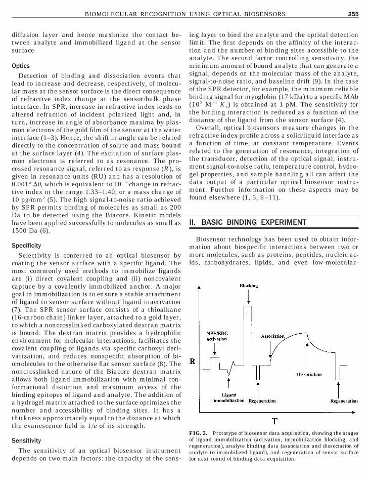
IG. 2. Prototype of biosensor data acquisition, showing the stagesf ligand immobilization (activation, immobilization blocking, and

egeneration), analyte binding data (association and dissociation ofnalyte to immobilized ligand), and regeneration of sensor surfaceor next round of binding data acquisition.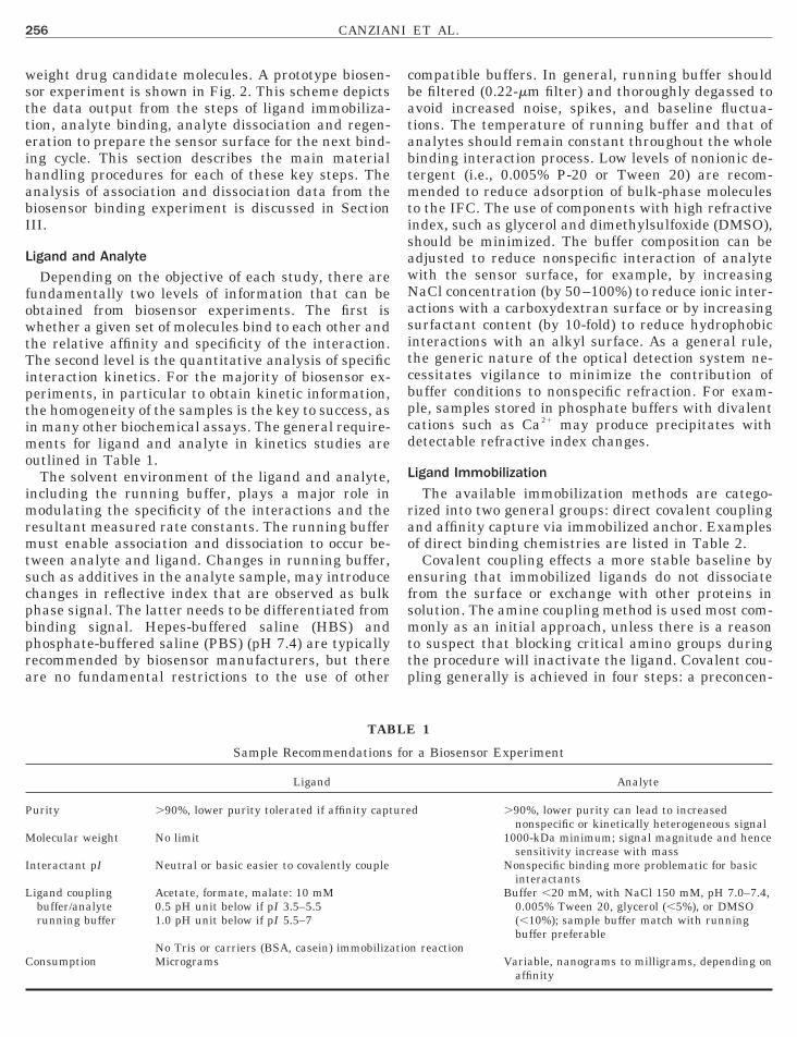

wstteihabI

L

fowtTiptimo

imrmtscpbpra

cbatabtmtisawNasitcbpcd

L

rao

efsmttp

P

M

I

L

C

256 CANZIANI ET AL.

eight drug candidate molecules. A prototype biosen-or experiment is shown in Fig. 2. This scheme depictshe data output from the steps of ligand immobiliza-ion, analyte binding, analyte dissociation and regen-ration to prepare the sensor surface for the next bind-ng cycle. This section describes the main materialandling procedures for each of these key steps. Thenalysis of association and dissociation data from theiosensor binding experiment is discussed in SectionII.

igand and Analyte

Depending on the objective of each study, there areundamentally two levels of information that can bebtained from biosensor experiments. The first ishether a given set of molecules bind to each other and

he relative affinity and specificity of the interaction.he second level is the quantitative analysis of specific

nteraction kinetics. For the majority of biosensor ex-eriments, in particular to obtain kinetic information,he homogeneity of the samples is the key to success, asn many other biochemical assays. The general require-

ents for ligand and analyte in kinetics studies areutlined in Table 1.The solvent environment of the ligand and analyte,

ncluding the running buffer, plays a major role inodulating the specificity of the interactions and the

esultant measured rate constants. The running bufferust enable association and dissociation to occur be-

ween analyte and ligand. Changes in running buffer,uch as additives in the analyte sample, may introducehanges in reflective index that are observed as bulkhase signal. The latter needs to be differentiated frominding signal. Hepes-buffered saline (HBS) andhosphate-buffered saline (PBS) (pH 7.4) are typicallyecommended by biosensor manufacturers, but therere no fundamental restrictions to the use of other

TAB

Sample Recommendations

Ligand

urity .90%, lower purity tolerated if affinity capt

olecular weight No limit

nteractant pI Neutral or basic easier to covalently couple

igand couplingbuffer/analyterunning buffer

Acetate, formate, malate: 10 mM0.5 pH unit below if pI 3.5–5.51.0 pH unit below if pI 5.5–7

No Tris or carriers (BSA, casein) immobiliza

onsumption Micrograms

ompatible buffers. In general, running buffer shoulde filtered (0.22-mm filter) and thoroughly degassed tovoid increased noise, spikes, and baseline fluctua-ions. The temperature of running buffer and that ofnalytes should remain constant throughout the wholeinding interaction process. Low levels of nonionic de-ergent (i.e., 0.005% P-20 or Tween 20) are recom-ended to reduce adsorption of bulk-phase molecules

o the IFC. The use of components with high refractivendex, such as glycerol and dimethylsulfoxide (DMSO),hould be minimized. The buffer composition can bedjusted to reduce nonspecific interaction of analyteith the sensor surface, for example, by increasingaCl concentration (by 50–100%) to reduce ionic inter-ctions with a carboxydextran surface or by increasingurfactant content (by 10-fold) to reduce hydrophobicnteractions with an alkyl surface. As a general rule,he generic nature of the optical detection system ne-essitates vigilance to minimize the contribution ofuffer conditions to nonspecific refraction. For exam-le, samples stored in phosphate buffers with divalentations such as Ca21 may produce precipitates withetectable refractive index changes.

igand Immobilization

The available immobilization methods are catego-ized into two general groups: direct covalent couplingnd affinity capture via immobilized anchor. Examplesf direct binding chemistries are listed in Table 2.Covalent coupling effects a more stable baseline by

nsuring that immobilized ligands do not dissociaterom the surface or exchange with other proteins inolution. The amine coupling method is used most com-only as an initial approach, unless there is a reason

o suspect that blocking critical amino groups duringhe procedure will inactivate the ligand. Covalent cou-ling generally is achieved in four steps: a preconcen-

1

a Biosensor Experiment

Analyte

d .90%, lower purity can lead to increasednonspecific or kinetically heterogeneous signal

1000-kDa minimum; signal magnitude and hencesensitivity increase with mass

Nonspecific binding more problematic for basicinteractants

Buffer ,20 mM, with NaCl 150 mM, pH 7.0–7.4,0.005% Tween 20, glycerol (,5%), or DMSO(,10%); sample buffer match with runningbuffer preferable

n reaction

LE

for

ure

tio

Variable, nanograms to milligrams, depending on

affinity

tdaNv(stp

cotcEttasmmgs(

sacsse

tnTanrT1ttbtcnttp

A

AD

t

257BIOMOLECULAR RECOGNITION USING OPTICAL BIOSENSORS

ration at the matrix to drive the ligand into the hy-rogel; activation (3–8 min); covalent bond formationt the same pH and at low ionic strength (,50 mMaCl or equivalent for other buffers); blocking of acti-

ated carboxyl groups that have not been hydrolyzed3–8 min); and regeneration of the immobilized ligandensor surface in preparation for adding analyte. Aypical sensorgram of immobilization by amine cou-ling is depicted in Fig. 2.Because the net charge of the most frequently used

arboxydextran matrix (Biacore) is negative, ligandsften are preconcentrated at a pH below their isoelec-ric point. Superactivation of surface carboxyls, by in-reasing the recommended concentrations of NHS/DC 5- to 10-fold, reduces the net negative charge of

he hydrogel and hence can regulate the preconcentra-ion effect. The slope of the increasing signal due toccumulation of mass in the preconcentration phasehould be linear; this slope enables an estimate to beade of the contact time required to obtain a predeter-ined number of resonance units of immobilized li-

and. Whichever method is employed to coat the sen-or, the coated surface should be washed thoroughlythe first regeneration step in Fig. 2) to eliminate non-

TAB

Examples of Ligand Im

Direct covalent coupling

vailable methods Amine couplingLigand thiol couplingSurface thiol couplingAldehyde coupling(See scheme for details)

dvantages Stable baseline after immobilizationisadvantages Less control of the ligand orientation

a NHS, N-hydroxysuccinimide; EDC, N-ethyl-N9-(dimethylaminoprophiothreitol; DTE, dithioerythritol.

pecifically immobilized ligand and to ensure that themount of immobilized ligand will remain relativelyonstant throughout the experiment. The constant re-ponse or R value of the coated and washed sensorurface becomes the baseline for subsequent bindingxperiments.The concentration of immobilized ligand may be es-

imated from the dimensions of the flow cell, the thick-ess of the hydrogel, and the baseline signal change.he SPR detection area is 0.224 mm2 (1.4 3 0.16 mm),nd the carboxydextran hydrogel height is 100 nm (20m in 150 mM NaCl) The R-to-mass correlation is 1esponse unit for each 1 pg/mm2 bound to the surface.hus, 1 RU is equivalent to a surface concentration of0 mg/liter. A 30-kDa protein immobilized at a concen-ration of 333 nmol/liter or 333 nM would be expectedo generate a signal of approximately 100 RU. Theaseline signal after the immobilization, also referredo as the immobilization level, represents the bindingapacity of the ligand. In general, to answer the “yes oro” question of whether the analyte binds specificallyo a given ligand, high immobilization may be advan-ageous to increase the signal. However, for the pur-ose of kinetic analysis, low immobilization levels offer

2

bilization Chemistriesa

Affinity capture example

Streptavidin (for biotinylated ligands)Anti-Fc (for MAbs)Anti-GST (for GST-tagged ligands)RNase S protein (for S-tagged ligands)Nickel chelate (for histidine-tagged ligands)Anti-Flag (for Flag sequence-tagged ligands)Better control of ligand orientation for optimal site exposureLess stable baseline

LE

mo

yl)carbodiimide; PDEA, 2-(2-pyridinyldithio)ethaneamine; DTT, di-

mdy

I

ttt(tsasiiotuak

bblscvtB

ttriagah

R

titnssmtpTwtmtpm

ec

A

B

H

I

C

M

258 CANZIANI ET AL.

ore reliable results for the kinetic analysis of theata. The effect of immobilization level in kinetic anal-sis is discussed in detail in Section III.

nteraction of Analyte with Immobilized LigandThe association and dissociation of an analyte with

he immobilized ligand are monitored by changes in Rhat occur in real time once the analyte has been in-roduced into the flow upstream of the sensor surfaceassociation phase in Fig. 2) and subsequently whenhe flow cell is washed with running buffer alone (dis-ociation phase in Fig. 2). In the association phase, thenalyte sample is injected over the surface at a con-tant flow rate for a defined contact time. Any massncrease on the surface resulting from ligand–analytenteraction is detected as an increase in response. Tobtain the maximum information about the interac-ion, a wide range of analyte concentrations should besed in each experiment. Testing different flow ratesnd contact times often provides additional valuableinetic information (see Section III for details).In the dissociation phase, a wash with the running

uffer is applied after the analyte sample injection haseen completed. The dissociation of analyte from theigand–analyte complex is detected as a decrease inignal due to loss of mass from the surface. The disso-iation phase is intended to remove all the nonco-alently bound material, allowing the baseline to re-urn to the initial value before the analyte injection.ecause the number of free sites increases with the

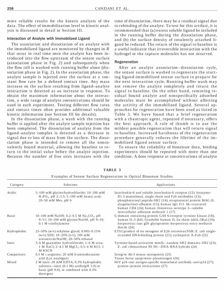
TAB

Examples of Sensor Surface Regen

Category Solutions

cidic 5–100 mM glycine/hydrochloride; 10–100 mMH3PO4, pH 2–3.5; 5–100 mM formic acid;20–50 mM Mes, pH 6

asic 10–100 mM NaOH; 0.2–0.5 M Na2CO3, pH9–11; 10–100 mM glycine/NaOH, pH 9–10;0.1 M triethylamine

ydrophobic 25–50% (w/v) ethylene glycol; 0.005–0.15%(w/v) SDS; 10–20% (v/v), 100 mMacetonitrile/NaOH; 20–50% ethanol

onic 3–6 M guanidine hydrochloride; 1–6 M urea;1 M NaCl; 2–4.5 M MgCl2; 0.5–4 M KCl; 3M KSCN

ompetitors 0.5 M L-arginine; 20 mM 6-aminohexanoicacid (Lys analogue)

ixed 2 M ionic–20 mM EDTA; 0.3% hydrophobicsolvents—ionic (0.1 M)–acidic(pH 5.0) or

basic (pH 9.0), or combined with 0.3%detergent

ime of dissociation, there may be a residual signal dueo rebinding of the analyte. To test for this artifact, it isecommended that (a) excess soluble ligand be includedn the running buffer during the dissociation phase,nd (b) the surface density of covalently attached li-and be reduced. The return of the signal to baseline isuseful indicator that irreversible interaction with theydrogel or the capture molecules has not occurred.

egenerationAfter an analyte association– dissociation cycle,

he sensor surface is washed to regenerate the start-ng ligand-immobilized sensor surface to prepare forhe next interaction cycle. Running buffer wash mayot remove the analyte completely and return theignal to baseline. On the other hand, removing re-idual bound analyte and nonspecifically adsorbedolecules must be accomplished without affecting

he activity of the immobilized ligand. Several ap-roaches for regeneration have been used as listed inable 3. We have found that a brief regenerationith a chaotropic agent, repeated if necessary, offers

he best approach. A rule of thumb is to use theildest possible regeneration that will return signal

o baseline. Increased harshness of the regenerationrocedure generally reduces the lifetime of the im-obilized ligand sensor surface.To ensure the reliability of biosensor data, binding

xperiments should be repeated with more than oneondition. A dose response at concentrations of analyte

3

tion in Optical Biosensor Studies

Applications

nterleukin-6 and soluble interleukin-6 receptor (12); lysozyme-D1.3 monoclonal, single chain and Fab antibodies (13);phosphotyrosyl peptide-SH2 (14); streptococcal protein MAG (S.dysgalactiae)–albumin (15); human IgG Fc1 Ab–truncatedhuman CD4 (16); human rhinovirus serotype 3—solubleintercellular adhesion molecule 1 (17)-domain containing protein GAS 6-receptor tyrosine kinase (18);human IL-5 (hIL-5)-soluble human IL-5a chain (shIL-5Ra) (19);herpesvirus coat gDt glycoprotein–herpesvirus entry mediatorHevAt (20)TS1:product of ets oncogene of E26 retrovirus/SSB: E. coli single-stranded DNA-binding protein (21); cyclosporin A–Fab (22)

yrosine-based activation motifs—tandem SH2 domains–SH2 (23);E. coli ribonuclease HI HI—DNA–RNA hybrids (24)

ntegrin Ab-3 mouse osteopontin (25)issue factor apoprotein–plasminogen (26)IV p24 coat antigen-specific monoclonal antibody–anti-p24 (27);protein–protein interactions (27)

LE

era

I

G

E

T

ITH

ocicdfot

I

W

tclmo

ctaf

tpc

mt

ab

Afiowa

K

m(0fm

ttct

coitotttadd

Fiia

259BIOMOLECULAR RECOGNITION USING OPTICAL BIOSENSORS

ver a range of several orders of magnitude will help toonfirm the maximum binding capacity (or saturabil-ty) of the surface. Negative and positive controls areritical additional measures of the reliability of bindingata. A reference surface is always needed to accountor and to minimize artifacts. Reruns of analyte peri-dically during a binding series ensure the integrity ofhe sensor surface.

II. OPTICAL BIOSENSOR DATA ANALYSIS

hat Can Be Learned Using an Optical Biosensor

Biosensor binding data are intrinsically informa-ion rich but need to be analyzed with caution to ex-lude artifacts and to ensure that the data are ana-yzed in the context of the most appropriate binding

odel. Several types of useful binding data may bebtained.a. Presence of an interaction. The sensor provides a

onvenient means to detect binding interactions be-ween analytes and immobilized ligands with smallmounts of interacting partners and without the needor either reactant to be labeled.

b. Multimolecular complexes. Binding can be de-ected of an analyte to a sensor surface that contains areexisting complex or between a preexisting analyteomplex and an immobilized ligand.

c. Kinetics. On and off rate constants can be deter-ined from the association and dissociation phases of

he binding sensorgram.

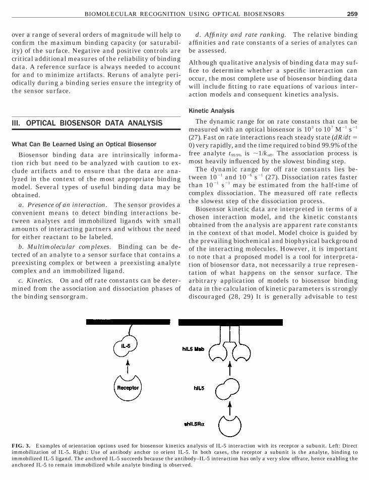
mmobilization of IL-5. Right: Use of antibody anchor to orient IL-5.mmobilized IL-5 ligand. The anchored IL-5 succeeds because the antibonchored IL-5 to remain immobilized while analyte binding is observed

d. Affinity and rate ranking. The relative bindingffinities and rate constants of a series of analytes cane assessed.

lthough qualitative analysis of binding data may suf-ce to determine whether a specific interaction canccur, the most complete use of biosensor binding dataill include fitting to rate equations of various inter-ction models and consequent kinetics analysis.

inetic Analysis

The dynamic range for on rate constants that can beeasured with an optical biosensor is 103 to 107 M21 s21

27). Fast on rate interactions reach steady state (dR/dt 5) very rapidly, and the time required to bind 99.9% of theree analyte t99.9% is ;1/koff. The association process isost heavily influenced by the slowest binding step.The dynamic range for off rate constants lies be-

ween 1021 and 1026 s21 (27). Dissociation rates fasterhan 1021 s21 may be estimated from the half-time ofomplex dissociation. The measured off rate reflectshe slowest step of the dissociation process.

Biosensor kinetic data are interpreted in terms of ahosen interaction model, and the kinetic constantsbtained from the analysis are apparent rate constantsn the context of that model. Model choice is guided byhe prevailing biochemical and biophysical backgroundf the interacting molecules. However, it is importanto note that a proposed model is a tool for interpreta-ion of biosensor data, not necessarily a true represen-ation of what happens on the sensor surface. Therbitrary application of models to biosensor bindingata in the calculation of kinetic parameters is stronglyiscouraged (28, 29) It is generally advisable to test

IG. 3. Examples of orientation options used for biosensor kinetics analysis of IL-5 interaction with its receptor a subunit. Left: Direct

In both cases, the receptor a subunit is the analyte, binding to

dy–IL-5 interaction has only a very slow offrate, hence enabling the.

ps

1b

T

Ittt

w

Hftkdcvss

a2

wds

dgmsiu(ge

C

EpvtmptonSb

m

F1t

260 CANZIANI ET AL.

redetermined models in biosensor kinetic studies,imilarly as would be done in enzyme kinetics (6, 28).The simplest model for a biosensor interaction is a

:1 binding between A, the analyte, and B, the immo-ilized ligand:

A 1 B L|;kon

koff

AB. [1]

he rate equation for the formation of AB complex is

d@AB#/dt 5 kon [A][B] 2 koff[AB]. [2]

n the context of biosensor terminology, B is immobilized onhe sensor surface, [B] is the baseline signal, and [AB] ishe complex formed, or R (response), at time t. Hence, inerms of the resonance signal change, the rate equation is

dR/dt 5 kon@A#~Rmax 2 R! 2 koffR, [3]

hich can be rearranged to

dR/dt 5 kon@A#Rmax 2 ~kon@A# 1 koff!R. [4]

ere, Rmax is the maximum binding signal of the sur-ace (or [Mw A/Mw B] * [RU A/RU B] * stoichiometry ofhe interaction). The term (k on[A] 1 k off) is defined ass. Hence, k s values can be obtained from the slopes ofR/dt versus R plots at various values of [A], and k on

an subsequently be determined from the slope of k s

ersus [A]. When R reaches its equilibrium or steady-tate value at any given [A], no further increase inignal is detected as a function of time. In the dissoci-

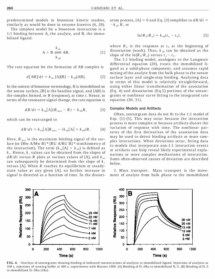
IG. 4. Overlays of sensorgrams showing binding of indicated concen00 s, injections of running buffer at 460 s, experiments with Biacore 1o immobilized IL-5Ra (18a).

tion process, [A] 5 0 and Eq. [3] simplifies to dR/dt 5k off R, or

ln~R0/Rn! 5 koff~tn 2 t0!, [5]

here R 0 is the response at t 0 at the beginning ofissociation (wash). Thus, k off can be obtained as thelope of the ln(R 0/Rn) versus tn2 t 0.The 1:1 binding model, analogous to the Langmuir

ifferential equation (20), treats the immobilized li-and as a solid-phase component, and assumes rapidixing of the analyte from the bulk phase to the sensor

urface layer and single-step binding. Analyzing datan terms of this model is relatively straightforward,sing either linear transformation of the associationEq. 4) and dissociation (Eq.5) portions of the sensor-rams or nonlinear curve fitting to the integrated ratequation (30, 31).

omplex Models and Artifacts

Often, sensorgram data do not fit to the 1:1 model ofqs. [1]–[5]. This may occur because the interactionrocess is more complex or because artifacts distort theariation of response with time. The nonlinear pat-erns of the first derivatives of the association dataay be used to detect binding artifacts or more com-

lex interactions. When deviations occur, fitting datao models that incorporate non-1:1 interaction eventsr artifacts can help reveal likely experimental expla-ations or more complex mechanisms of interaction.ome often-observed causes of deviation are describedelow.

1. Mass transport. Mass transport is the move-ent of analyte from bulk phase to the immobilized

trations of analytes to immobilized ligand. Injections of analytes at000. (A) Binding of IL-5Ra to immobilized IL-5. (B) Binding of IL-5

lpocaatweprpsw

dacfslmsdn

osstwsltla

cmbI

vfpmi

tataeciosmbdimplctMftkt[

FaB

261BIOMOLECULAR RECOGNITION USING OPTICAL BIOSENSORS

igand on the sensor solid-phase surface. If this trans-ort process is slow compared with the association ratef analyte, or if the transport on dissociation is slowompared with the dissociation rate of analyte, thepparent rates determined by biosensor interactionnalysis will be artifactually slow (20, 32). Accordingly,he plots of dR/dt versus R or of ln(dR/dt) versus timeill show convex nonlinearity. k on and k off are under-stimated in presence of mass transport. Mass trans-ort may be minimized by increasing the flow rate, toeduce the unstirred layer between bulk and solidhases, or by using low ligand densities, to minimizeteric hindrance and maximize ligand accessibilityithin the dextran layer (33).2. Linked interactions. Linked interactions may

erive from such events as postbinding association ofdditional analyte and postbinding conformationalhanges that cause increased affinity. Data deviaterom the bivalent model because in these circum-tances the equilibrium between bound and free ana-yte changes with time. Linear dR/dt transformations

ay result in concave rather than straight lines. Ifuch postbinding events are suspected, sensorgramata should be fitted to a rate equation for appropriateon-1:1 interaction models (29, 34).3. Ligand heterogeneity. If ligands with more than

ne interaction rate are present together on the sameensor surface due to heterogeneity of the initial ligandample or heterogeneity imposed during immobiliza-ion, the rate of response increase on analyte bindingill be the sum of more than one type of interaction. In

uch circumstances, linearizing replots will be curvi-inear. The possibility of parallel, nonequal interac-ions can be tested by trials over a wide range of ana-yte concentrations. At low concentrations, the high-ffinity process will predominate, whereas at high

IG. 5. Linearized association phases of sensorgrams from Fig. 4 acconalyte concentration; slopes of these plots provide a graphical meansinding of IL-5 to immobilized IL-5Ra (18a).

oncentrations, the low-affinity process will becomeore evident. Ligand heterogeneity can be minimized

y employing a capture (anchored ligand, see SectionV) immobilization method (29).

4. Avidity effects with multivalent analyte. Multi-alent analytes such as antibodies will bind with dif-erent affinities depending on the number of sites thatarticipate in ligand binding. If the antigen is mono-eric, complex kinetics can be overcome by immobiliz-

ng the analyte and using the antigen as analyte (35).

To test alternative models, the first step is to identifyhe simplest model consistent with what is knownbout the molecular system. If the data cannot be fit byhis simplest model, the first recourse is to eliminate ort least minimize potential experimental artifacts, forxample, by reducing ligand density (to reduce theontribution of mass transport) and by improving pre-mmobilization purity of ligand (to reduce the chancesf ligand heterogeneity). If such artifact-eliminatingteps fail to improve fit of data to a simple bindingodel, more complex models can be tested. Models can

e generated by numerical integration of the ordinaryifferential equations that describe complex, multistepnteractions between two molecules (20, 34). Data sets

ay be simulated using these models, for example, forostbinding conformational change, postbinding ana-yte aggregation, or multivalent avidity effects. Asso-iation constants above 5 3 105 M21 s21 are subject tohe effects of mass transport at the sensor surface (36).odels based on the integration of more complex dif-

erential equations that take into account the km (massransport constant) for the analyte (6, 27, 28) permitinetic parameters to be estimated in situations wherehe interactions are limited by mass transportCLAMP (37), BIA evaluation 3.0 (38)].

rding to Eq. [3]. Insets are plots of k s values (5 k on[A] 1 k off) versusto determine k on. (A) Binding of IL-5Ra to immobilized IL-5. (B)

S

ratavd

IU

stdt

aSA

papahcaiyIcs

bimmca

K

baotUwT4iaittt

dFri5ssavkt

FatI

262 CANZIANI ET AL.

teady-State Binding AnalysisSensorgram data can be used to evaluate equilib-

ium binding affinity constants independent of kineticnalysis of individual rate constants. In this analysis,he steady-state amount bound at each of a set ofnalyte concentrations is determined by the plateau Ralue reached during the association phase, when dR/t 5 0 (39).

V. EXAMPLES OF INTERACTION ANALYSISSING OPTICAL BIOSENSORS

Several examples are given below of binding analy-es carried out with optical biosensors. They are choseno exemplify the major types of assay configurations,ata analysis approaches, and information obtained byhis technology.

. Interleukin-5 Receptor Recognition: Kinetic andteady-State Analyses and Their Role in Mutagenicnalysis of Recognition MechanismHuman interleukin-5 (hIL-5) is the major hemato-

oietin responsible for differentiation, proliferation,nd activation of eosinophils. IL-5 is a homodimericrotein dominated by two four-helix bundle units andcts on eosinophils through a cell surface receptor. Theuman IL-5 receptor (hIL-5R) contains a and bc

hains, with a primarily responsible for ligand bindingnd bc for signal transduction. Major recent advancesn mutagenic approaches and tools for structure anal-sis enable determination of recognition elements inL-5 and receptor subunit ectodomains and how theseontrol functional recruitment of a and bc receptorubunits. Optical biosensor interaction analysis has

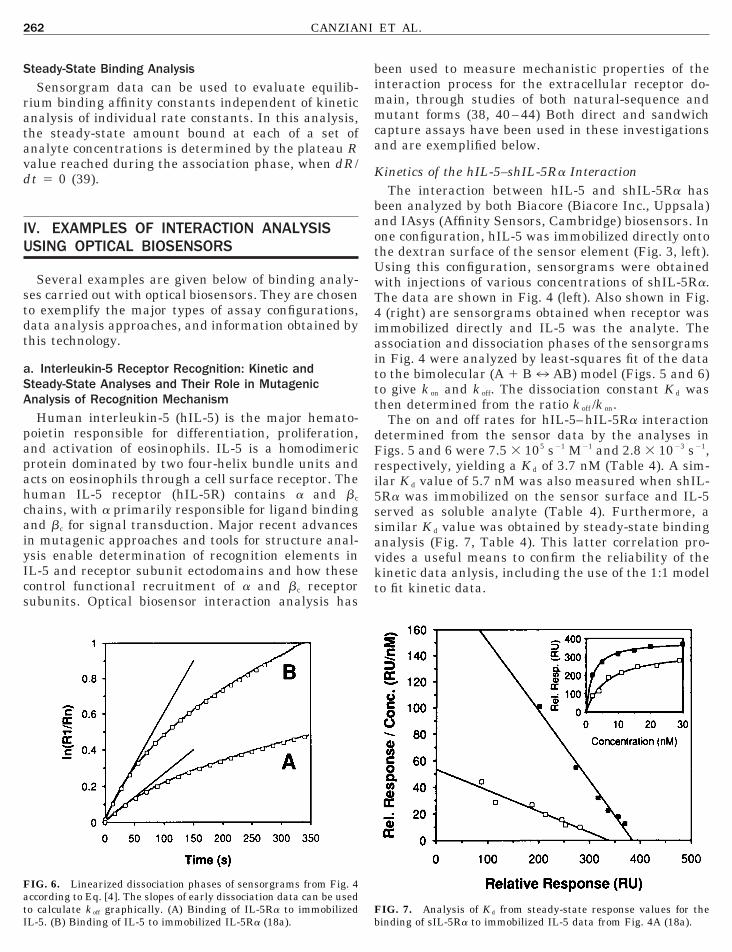
ccording to Eq. [4]. The slopes of early dissociation data can be usedo calculate k off graphically. (A) Binding of IL-5Ra to immobilizedL-5. (B) Binding of IL-5 to immobilized IL-5Ra (18a).

Fb

een used to measure mechanistic properties of thenteraction process for the extracellular receptor do-

ain, through studies of both natural-sequence andutant forms (38, 40–44) Both direct and sandwich

apture assays have been used in these investigationsnd are exemplified below.

inetics of the hIL-5–shIL-5Ra InteractionThe interaction between hIL-5 and shIL-5Ra has

een analyzed by both Biacore (Biacore Inc., Uppsala)nd IAsys (Affinity Sensors, Cambridge) biosensors. Inne configuration, hIL-5 was immobilized directly ontohe dextran surface of the sensor element (Fig. 3, left).sing this configuration, sensorgrams were obtainedith injections of various concentrations of shIL-5Ra.he data are shown in Fig. 4 (left). Also shown in Fig.(right) are sensorgrams obtained when receptor was

mmobilized directly and IL-5 was the analyte. Thessociation and dissociation phases of the sensorgramsn Fig. 4 were analyzed by least-squares fit of the datao the bimolecular (A 1 B7 AB) model (Figs. 5 and 6)o give k on and k off. The dissociation constant K d washen determined from the ratio k off /k on.

The on and off rates for hIL-5–hIL-5Ra interactionetermined from the sensor data by the analyses inigs. 5 and 6 were 7.5 3 105 s21 M21 and 2.8 3 1023 s21,espectively, yielding a K d of 3.7 nM (Table 4). A sim-lar K d value of 5.7 nM was also measured when shIL-Ra was immobilized on the sensor surface and IL-5erved as soluble analyte (Table 4). Furthermore, aimilar K d value was obtained by steady-state bindingnalysis (Fig. 7, Table 4). This latter correlation pro-ides a useful means to confirm the reliability of theinetic data anlysis, including the use of the 1:1 modelo fit kinetic data.

IG. 6. Linearized dissociation phases of sensorgrams from Fig. 4

IG. 7. Analysis of K d from steady-state response values for theinding of sIL-5Ra to immobilized IL-5 data from Fig. 4A (18a).

omtaihcahrdddaompdda

B

sHiam(iabhia

TtdtdS(tt

aoTltmashcmatmbpTea(airrhcalcise5

b

taeuct

IsI

b

3

263BIOMOLECULAR RECOGNITION USING OPTICAL BIOSENSORS

The rates determined are comparable to the on andff rates of interaction between human growth hor-one (hGH) and human growth hormone-binding pro-

ein hGHbp (45). This is not surprising in that hGHlso possesses a four-helix bundle structure very sim-lar to that of hIL-5. While electrostatic interactionsave been suggested to be the most important side-hain determinants in guiding hGH to hGHbp (i.e.,ffecting k on), they may have little effect on the k on ofIL-5 binding to shIL-5Ra since the association rateemains constant between pH 5.5 and 10.5 (18a). Theissociation rate of hIL-5–shIL-5Ra is also indepen-ent of pH in the pH range 6.5–9.5, but increasesramatically below pH 6.5 and above pH 9.5. The rel-tive insensitivity of k on to pH and greater sensitivityf k off suggest a model in which the association processay be driven primarily by generic apolar interactions,

ossibly through multiple docking modes, whereas theissociation process is controlled by a more specific,irectional set of interactions which here appear to be,t least in part, electrostatic.

inding Analysis of hIL-5 Mutants and Mapping theBinding Sites for shIL-5Ra on hIL-5

Although the crystal structure of hIL-5 has beenolved, that of the receptor–cytokine complex has not.ence, structural understanding of the IL-5–IL-5Ra

nteraction has relied heavily on evaluating the inter-ction properties of mutated proteins. Data from frag-ent shuffling experiments suggest that both helices A

residues 7–26) and D (residues 93–110) contributemportant components to receptor binding sites for the

and bc chains (47–50). It has also been suggested,ased on the data from chimeric molecules of mouse/uman IL-5, that the carboxyl terminal region of IL-5

s capable of interacting directly with IL-5 receptornd, indeed, confers the species specificity of IL-5 (48).

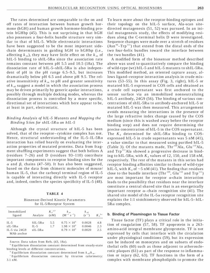
TABLE 4

Biosensor-Derived Kinetic Parametersfor IL-5/Receptor System

Immobilizedligand Analyte

Kda,b

(nM)k on

(M21 s21)k off

(s21) K db,c

L-5 SIL-5Ra 5.5 0.75 3 106 0.0028 4.8IL-5Ra IL-5 1.7 1.98 3 106 0.0046 2.3L-5 via 24G9

MAb anchorsIL-5Ra 0.79 3 106 0.0020 2.5

Source. Data taken from Refs. (43, 18a).a Equilibrium dissociation constant determined from steady-state

inding levels at different concentrations.

rtc

b Equilibrium dissociation constant determined from k off/k on.c Equilibrium dissociation constant by titration calorimetry:

.1 nM.

o learn more about the receptor-binding epitopes andheir topology on the hIL-5 surface, Ala-scan site-irected mutagenesis (51, 52) was pursued. In an ini-ial mutagenesis study, the effects of modifying resi-ues along the C-terminal helix D were investigated.equence changes were made over a stretch of residues

Asn94–Trp111) that extend from the distal ends of thewo four-helix bundles toward the interface betweenhe two bundles (41).

A modified form of the biosensor method describedbove was used to quantitatively compare the bindingf wild-type (wt) hIL-5 and hIL-5 mutants to shIL-5Ra.his modified method, an oriented capture assay, al-

ows ligand–receptor interaction analysis in crude mix-ures (53–55). In this assay (Fig. 3, right), hIL-5 orutated hIL-5 expressed in COS cells and obtained ascrude cell supernatant was first anchored to the

ensor surface via an immobilized nonneutralizingIL-5 antibody, 24G9 (56). The binding of various con-entrations of shIL-5Ra to antibody-anchored hIL-5 orutated hIL-5 was then measured. This arrangement

voids measuring the interactions in the presence ofhe large refractive index change caused by the COSedium (since this is washed away before the receptor

inding step) and does not require determining therecise concentration of hIL-5 in the COS supernatant.he K d determined for shIL-5Ra binding to COS-xpressed hIL-5 in crude supernatants was 5 nM (41),value similar to that measured using purified hIL-5

Table 3). Of the mutants made, Thr109Ala, Glu110Ala,nd Trp111Ala showed a progressive decrease in bind-ng to hIL-5Ra, with K d values of 12, 150, and 158 nM,espectively. The rest of the mutants in this series hadeceptor binding affinities similar to those of wild-typeIL-5, with K d of ;5 nM (41). The finding that residueslose to the bundle interface (Thr109, Glu110 and Trp111)re most important for receptor a-chain interactioneads to the possibility that residues near the interfaceonstitute a central shared site that is an energeticallymportant receptor a–chain recognition site (41). Thehared site model of the IL-5a receptor recognition sitexplains the 1:1 stoichiometry observed for hIL-5–hIL-Ra complex.

. Binding of Plasminogen to Tissue Factor

Tissue factor (TF) plays a critical role in the initia-ion of coagulation (57, 58). TF apoprotein is a 263-mino-acid integral membrane glycoprotein. TF is notxpressed by cells that interface with the circulationnder physiological conditions (59), but its expressionan be induced on monocytes and on subsets of endo-helial cells (60) such as those adjacent to atheroscle-otic plaques (61) as part of the response to inflamma-

ion or injury (62, 63). TF functions in the form of aomplex with membrane phospholipids to promote the

abdebaTplTypb

D

rbTto8ia[dlbm

dcm

1oeoet

M

iVfmtewFcsmffirnab

R

mTfi

Faai

264 CANZIANI ET AL.

ctivation of factors VII, X, and IX. The presence ofoth components is required under physiological con-itions for optimal procoagulant activity (64–67). Sev-ral observations suggest potentially important linksetween the initiation of coagulation by tissue factornd the dissolution of fibrin clots by plasmin (68).hese findings have led to the question of whetherlasminogen binds to TF and whether TF may modu-ate the expression of plasminogen activator activity.his, in turn, has led to biosensor-based binding anal-ses to obtain direct evidence for TF interaction withlasminogen and the possibility of a three-way complexetween TF, plasminogen, and factor VII.

etection of the Plasminogen–Tissue FactorInteraction

To determine whether plasminogen interacts di-ectly with tissue factor, the ability of plasminogen toind to a soluble, immobilized fragment of recombinantF apoprotein, comprising the extracellular domain ofhe protein (amino acids 1–219), was evaluated usingptical biosensor interaction analysis. As shown in Fig.(left), plasminogen was found to bind to this fragment

n a dose-dependent manner. Linearization of both thessociation and dissociation phases according to Eqs.4] and [5], respectively, showed that these processesid not fit strictly to a single bimolecular process. Non-inear dR/dt plots (Fig. 8, right) could reflect multipleinding sites with different affinities, cooperativity, orore complex models.To make approximations of binding constants, the

R/dt plots were divided into single fast and slowomponents (components 1 and 2, respectively), in aanner used previously (17). Linear fits of components

poprotein was immobilized and plasminogen at indicated concentratissociation phase of sensorgram at 1 mM showing nonlinear behavior ofndependently to obtain estimates of rate parameters. Reproduced, wit

and 2 to Eq. [4] yielded k s plots that led to k on valuesf 4 3 104 and 2 3 103 M21 s21, respectively. Fitting thearly dissociation data to Eq. [5] led to a calculated k off

f 3.8 3 1023 s21. From these linear fits, apparentquilibrium K d values of 100 nM and 2 mM were ob-ained for components 1 and 2, respectively.

ultimolecular Complexes Involving Plasminogen,TF, and Factor VIIa

Optical biosensor analysis also was used to exam-ne whether plasminogen had an effect on factor (F)II and FVIIa binding to TF apoprotein. FVIIa was

ound to bind to immobilized TF extracellular do-ain by biosensor analysis (data not shown), consis-

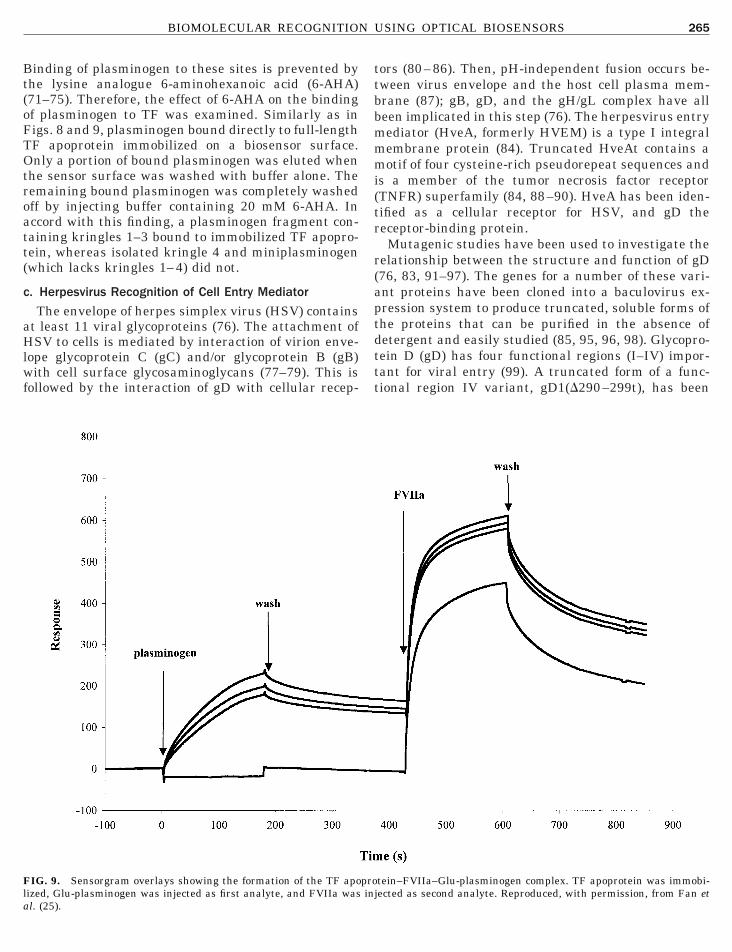
ent with previously published results (69, 70). Theffect of plasminogen on the TF–FVIIa interactionas evaluated by a sequential assay. As shown inig. 9, preinjection of plasminogen at increasing con-entrations did not significantly reduce the extent ofubsequent FVIIa binding, as judged by the maxi-um response signal after FVIIa injection, corrected

or the signal due to bound plasminogen. A similarnding was observed when the order of injection waseversed, i.e., FVIIa followed by plasminogen (dataot shown). Hence, plasminogen and FVII do notppear to block each other’s binding to TF and likelyind at independent sites.

ole of Kringles in the Binding of Plasminogen to TF

The plasminogen molecule contains five kringle do-ains each of which contains a lysine binding site.hese kringles mediate the binding of plasminogen tobrin, to other proteins such as Lp(a), and to cells.

IG. 8. Left: Sensorgram overlays showing the dose responses for binding of plasminogen to soluble recombinant TF apoprotein. TF

ons was injected at 0 time as analyte. Right: Linearization plot ofdR/dt data and way in which the two apparent phases were fitted

h permission, from Fan et al. (25).

Bt(oFTOtroatt(

c

aHlwf

ttbbmmmi(tr

r(aptdttt

Fla

265BIOMOLECULAR RECOGNITION USING OPTICAL BIOSENSORS

inding of plasminogen to these sites is prevented byhe lysine analogue 6-aminohexanoic acid (6-AHA)71–75). Therefore, the effect of 6-AHA on the bindingf plasminogen to TF was examined. Similarly as inigs. 8 and 9, plasminogen bound directly to full-lengthF apoprotein immobilized on a biosensor surface.nly a portion of bound plasminogen was eluted when

he sensor surface was washed with buffer alone. Theemaining bound plasminogen was completely washedff by injecting buffer containing 20 mM 6-AHA. Inccord with this finding, a plasminogen fragment con-aining kringles 1–3 bound to immobilized TF apopro-ein, whereas isolated kringle 4 and miniplasminogenwhich lacks kringles 1–4) did not.

. Herpesvirus Recognition of Cell Entry Mediator

The envelope of herpes simplex virus (HSV) containst least 11 viral glycoproteins (76). The attachment ofSV to cells is mediated by interaction of virion enve-

ope glycoprotein C (gC) and/or glycoprotein B (gB)ith cell surface glycosaminoglycans (77–79). This is

ollowed by the interaction of gD with cellular recep-

IG. 9. Sensorgram overlays showing the formation of the TF apoproized, Glu-plasminogen was injected as first analyte, and FVIIa was injl. (25).

ors (80–86). Then, pH-independent fusion occurs be-ween virus envelope and the host cell plasma mem-rane (87); gB, gD, and the gH/gL complex have alleen implicated in this step (76). The herpesvirus entryediator (HveA, formerly HVEM) is a type I integralembrane protein (84). Truncated HveAt contains aotif of four cysteine-rich pseudorepeat sequences and

s a member of the tumor necrosis factor receptorTNFR) superfamily (84, 88–90). HveA has been iden-ified as a cellular receptor for HSV, and gD theeceptor-binding protein.Mutagenic studies have been used to investigate the

elationship between the structure and function of gD76, 83, 91–97). The genes for a number of these vari-nt proteins have been cloned into a baculovirus ex-ression system to produce truncated, soluble forms ofhe proteins that can be purified in the absence ofetergent and easily studied (85, 95, 96, 98). Glycopro-ein D (gD) has four functional regions (I–IV) impor-ant for viral entry (99). A truncated form of a func-ional region IV variant, gD1(D290–299t), has been

tein–FVIIa–Glu-plasminogen complex. TF apoprotein was immobi-ected as second analyte. Reproduced, with permission, from Fan et

s(etHgwi

ob

G

cHg3tgwi(ct

Ftmdswcfi

Fgt 10H gDi

ggggggg

266 CANZIANI ET AL.

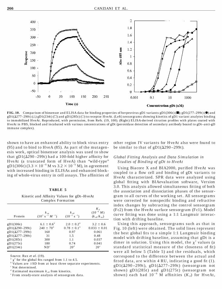
hown to have an enhanced ability to block virus entry95) and to bind to HveA (85). As part of the mutagen-sis work, optical biosensor analysis was used to showhat gD1(D290–299t) had a 100-fold higher affinity forveAt (a truncated form of HveA) than “wild-type”

D1(306t) (3.3 3 1028 M vs 3.2 3 1026 M), in agreementith increased binding in ELISAs and enhanced block-

ng of whole-virus entry in cell assays. The affinities of

IG. 10. Comparison of biosensor and ELISA data for binding propeD1(D277–290t) (‚) gD1(234t) (h) and gD1(285t) (E) to receptor HveAo immobilized HveAt. Reproduced, with permission, from Refs. (19,veAt in PBS, blocked and incubated with various concentrations of

mmune complex).

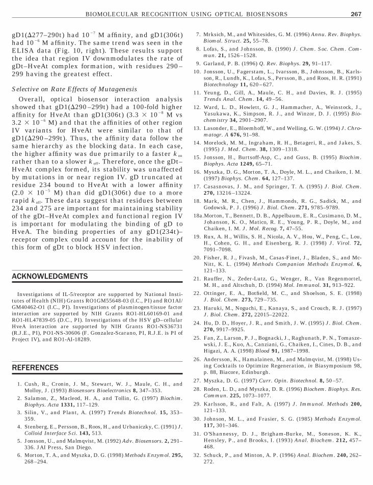
TABLE 5

Kinetic and Affinity Values for gDt–HveAtComplex Formation

Proteink on

(103 s21 M21)k off

(1022 s21)

K d

(1026 M)(k off /k on)

D1(306t) 6.1 6 0.6b 2.0 6 0.2b 3.2 6 0.6D1(D290–299t) 240 6 70b 0.78 6 0.1b 0.033 6 0.01D1(D277–299t) 160 0.97 0.061D1(D277–290t) 31 1.5 0.48D1(285t) 300 1.1 0.037D1(275t) 180 0.74 0.041D1(234t) NDc 20d 20e

Source. Rux et al. (19).a x2 for the global fits ranged from 1.1 to 4.5.b Values are 6SD from at least three separate experiments.

g

ss

c Not determined.d Estimated maximum k off from kinetics.e From steady-state analysis of sensorgram data.

ther region IV variants for HveAt also were found toe similar to that of gD1(D290–299t).

lobal Fitting Analysis and Data Simulation inStudies of Binding of gDt to HveAt

Using Biacore X and BIA2000, purified HveAt wasoupled to a flow cell and binding of gDt variants toveAt characterized. SPR data were analyzed using

lobal fitting with BIAevaluation software, Version.0. This analysis allowed simultaneous fitting of bothhe association and dissociation phases of the sensor-ram to all curves of the working set. All sensorgramsere corrected for nonspecific binding and refractive

ndex changes by subtracting the control sensorgramFc2) from the HveAt surface sensorgram (Fc1). Modelurve fitting was done using a 1:1 Langmuir interac-ion with drifting baseline.

Using this approach, sensorgrams such as that inig. 10 (left) were obtained. The solid lines representhe best global fits to a simple 1:1 Langmuir bindingodel with drifting baseline, assuming that gDt is a

imer in solution. Using this model, the x2 values (atandard statistical measure of the closeness of fit)ere all below 5 (Table 5) and the residuals, which

orrespond to the difference between the actual andtted data, are within 4 RU, indicating a good fit (1).

es of herpesvirus gD1 variants gD1(306t) (■); gD1(277–299t) (F) and(Left) sensorgrams showing kinetics of gD1 variant analytes binding0). (Right) ELISA-derived titration profiles with plates coated witht (peroxidase detection of secondary antibody bound to gDt–anti-gD

rtit.

D1(D290 –299t), gD1(D277–299t) (sensorgram nothown) gD1(285t) and gD1(275t) (sensorgram nothown) each had 1028 M affinities (K d) for HveAt,

ghEtg2

S

sa3IgstrHbr(r2oiHrt

A

tGiRH(P

R

267BIOMOLECULAR RECOGNITION USING OPTICAL BIOSENSORS

D1(D277–290t) had 1027 M affinity, and gD1(306t)ad 1026 M affinity. The same trend was seen in theLISA data (Fig. 10, right). These results support

he idea that region IV downmodulates the rate ofDt–HveAt complex formation, with residues 290 –99 having the greatest effect.

elective on Rate Effects of MutagenesisOverall, optical biosensor interaction analysis

howed that gD1(D290 –299t) had a 100-fold higherffinity for HveAt than gD1(306t) (3.3 3 1028 M vs.2 3 1026 M) and that the affinities of other regionV variants for HveAt were similar to that ofD1(D290 –299t). Thus, the affinity data follow theame hierarchy as the blocking data. In each case,he higher affinity was due primarily to a faster k on

ather than to a slower k off. Therefore, once the gDt–veAt complex formed, its stability was unaffectedy mutations in or near region IV. gD truncated atesidue 234 bound to HveAt with a lower affinity2.0 3 1025 M) than did gD1(306t) due to a moreapid k off. These data suggest that residues between34 and 275 are important for maintaining stabilityf the gDt–HveAt complex and functional region IVs important for modulating the binding of gD toveA. The binding properties of any gD1(234t)–

eceptor complex could account for the inability ofhis form of gDt to block HSV infection.

CKNOWLEDGMENTS

Investigations of IL-5/receptor are supported by National Insti-utes of Health (NIH) Grants RO1GM55648-03 (I.C., PI) and RO1AI/M40462-O1 (I.C., PI). Investigations of plasminogen/tissue factor

nteraction are supported by NIH Grants RO1-HL60169-01 andO1-HL47839-05 (D.C., PI). Investigations of the HSV gD–cellularveA interaction are supported by NIH Grants RO1-NS36731

R.J.E., PI), PO1-NS-30606 (F. Gonzalez-Scarano, PI, R.J.E. is PI ofroject IV), and RO1-AI-18289.

EFERENCES

1. Cush, R., Cronin, J. M., Stewart, W. J., Maule, C. H., andMolloy, J. (1993) Biosensors Bioelectronics 8, 347–353.

2. Salamon, Z., Macleod, H. A., and Tollin, G. (1997) Biochim.Biophys. Acta 1331, 117–129.

3. Silin, V., and Plant, A. (1997) Trends Biotechnol. 15, 353–359.

4. Stenberg, E., Persson, B., Roos, H., and Urbaniczky, C. (1991) J.Colloid Interface Sci. 143, 513.

5. Jonsson, U., and Malmqvist, M. (1992) Adv. Biosensors. 2, 291–

336. JAI Press, San Diego.

6. Morton, T. A., and Myszka, D. G. (1998) Methods Enzymol. 295,268–294.

7. Mrksich, M., and Whitesides, G. M. (1996) Annu. Rev. Biophys.Biomol. Struct. 25, 55–78.

8. Lofas, S., and Johnsson, B. (1990) J. Chem. Soc. Chem. Com-mun. 21, 1526–1528.

9. Garland, P. B. (1996) Q. Rev. Biophys. 29, 91–117.10. Jonsson, U., Fagerstam, L., Ivarsson, B., Johnsson, B., Karls-

son, R., Lundh, K., Lofas, S., Persson, B., and Roos, H. R. (1991)Biotechnology 11, 620–627.

11. Yeung, D., Gill, A., Maule, C. H., and Davies, R. J. (1995)Trends Anal. Chem. 14, 49–56.

12. Ward, L. D., Howlett, G. J., Hammacher, A., Weinstock, J.,Yasukawa, K., Simpson, R. J., and Winzor, D. J. (1995) Bio-chemistry 34, 2901–2907.

13. Lasonder, E., Bloemhoff, W., and Welling, G. W. (1994) J. Chro-matogr. A 676, 91–98.

14. Morelock, M. M., Ingraham, R. H., Betageri, R., and Jakes, S.(1995) J. Med. Chem. 38, 1309–1318.

15. Jonsson, H., Burtsoff-Asp, C., and Guss, B. (1995) Biochim.Biophys. Acta 1249, 65–71.

16. Myszka, D. G., Morton, T. A., Doyle, M. L., and Chaiken, I. M.(1997) Biophys. Chem. 64, 127–137.

17. Casasnovas, J. M., and Springer, T. A. (1995) J. Biol. Chem.270, 13216–13224.

18. Mark, M. R., Chen, J., Hammonds, R. G., Sadick, M., andGodowsk, P. J. (1996) J. Biol. Chem. 271, 9785–9789.

18a.Morton, T., Bennett, D. B., Appelbaum, E. R., Cusimano, D. M.,Johanson, K. O., Matico, R. E., Young, P. R., Doyle, M., andChaiken, I. M. J. Mol. Recog. 7, 47–55.

19. Rux, A. H., Willis, S. H., Nicola, A. V., Hou, W., Peng, C., Lou,H., Cohen, G. H., and Eisenberg, R. J. (1998) J. Virol. 72,7091–7098.

20. Fisher, R. J., Fivash, M., Casas-Finet, J., Bladen, S., and Mc-Nitt, K. L. (1994) Methods Companion Methods Enzymol. 6,121–133.

21. Rauffer, N., Zeder-Lutz, G., Wenger, R., Van Regenmortel,M. H., and Altschuh, D. (1994) Mol. Immunol. 31, 913–922.

22. Ottinger, E. A., Botfield, M. C., and Shoelson, S. E. (1998)J. Biol. Chem. 273, 729–735.

23. Haruki, M., Noguchi, E., Kanaya, S., and Crouch, R. J. (1997)J. Biol. Chem. 272, 22015–22022.

24. Hu, D. D., Hoyer, J. R., and Smith, J. W. (1995) J. Biol. Chem.270, 9917–9925.

25. Fan, Z., Larson, P. J., Bognacki, J., Raghunath, P. N., Tomasze-wski, J. E., Kuo, A., Canziani, G., Chaiken, I., Cines, D. B., andHigazi, A. A. (1998) Blood 91, 1987–1998.

26. Andersson, K., Hamalainen, M., and Malmqvist, M. (1998) Us-ing Cocktails to Optimize Regeneration, in Biasymposium 98,p. 88, Biacore, Edinburgh.

27. Myszka, D. G. (1997) Curr. Opin. Biotechnol. 8, 50–57.

28. Roden, L. D., and Myszka, D. R. (1996) Biochem. Biophys. Res.Commun. 225, 1073–1077.

29. Karlsson, R., and Falt, A. (1997) J. Immunol. Methods 200,121–133.

30. Johnson, M. L., and Frasier, S. G. (1985) Methods Enzymol.117, 301–346.

31. O’Shannessy, D. J., Brigham-Burke, M., Soneson, K. K.,Hensley, P., and Brooks, I. (1993) Anal. Biochem. 212, 457–

468.

32. Schuck, P., and Minton, A. P. (1996) Anal. Biochem. 240, 262–272.

268 CANZIANI ET AL.

33. Karlsson, R., Roos, H., Fagerstam, L., and Persson, B. (1994)Methods Companion Meth. Enzymol. 6, 99–110.

34. Morton, T. A., Myszka, D. A., and Chaiken, I. M. (1995) Anal.Biochem. 227, 176–185.

35. Karlsson, R., Mo, J. A., and Holmdahl, R. (1995) J. Immunol.Methods 188, 63–71.

36. Myszka, D. G., He, X., Dembo, M., Morton, T. A., and Goldstein,B. (1998) Biophys. J. 75, 583–594.

37. Morton, T. (1995) http://www.hci.utah.edu/groups/biacore.38. Biacore, I. (1997) http://www.biacore.comc.39. Myszka, D. G., Jonsen, M. D., and Graves, B. J. (1998) Anal.

Biochem. 265, 326–330.40. Morton, T., Bennett, D. B., Appelbaum, E. R. D. C., Johanson,

K. O., Matico, R. E., Young, P. R., Doyle, M. L., and Chaiken,I. M. (1994) J. Mol. Recog. 7, 47–55.

41. Morton, T., Li, J., Cook, R., and Chaiken, I. M. (1995) Proc.Natl. Acad. Sci. USA 92, 10879–10883.

42. Li, J., Cook, R., Dede, K., and Chaiken, I. (1996) J. Biol. Chem.271, 1817–1820.

43. Li, J., Cook, R., and Chaiken, I. (1996) J. Biol. Chem. 271,31729–31734.

44. Li, J., Cook, R., Hensley, P., Doyle, M., McNulty, D.,and Chaiken, I. (1997) Proc. Natl. Acad. Sci. USA 94, 6694 –6699.

45. Cunningham, B. C., and Wells, J. A. (1993) J. Mol. Biol. 234,554–563.

46. Reference deleted in proofs.47. Kodama, S., Tsuruoka, N., and Tsujimoto, M. (1991) Biochem.

Biophys. Res. Commun. 178, 514–519.48. McKenzie, A. N. J., Barry, S. C., Strath, M., and Sanderson,

C. J. (1991) EMBO J. 10, 1193–1199.49. Shanafelt, A. B., Miyajima, A., Kitamura, T., and Kastelein,

R. A. (1991) EMBO J. 10, 4105–4112.50. Goodall, G. J., Bagley, C. J., Vadas, M. A., and Lopez, A. F.

(1993) Growth Factors 8, 87–97.51. Cunningham, B. C., and Wells, J. A. (1989) Science 244, 1081–

1085.52. Cunningham, B. C., Jhurani, P., Ng, P., and Wells, J. A. (1989)

Science 243, 1330–1336.53. Fagerstam, L. G., and Karlsson, R. (1994) in Immunochemistry,

pp. 949–970.54. Bennett, D. B., Morton, T. A., Breen, A. L., Hertzberg, R.,

Cusimano, D. M., Appelbaum, E. R., McDonnell, P., Young,P. R., Matico, R. E., Johanson, K., and Chaiken, I. M. (1995) J.Mol. Recog. 8, 52.

55. Bennett, M. J., Schlunegger, M. P., and Eisenberg, D. (1995)Protein Sci. 4, 2455–2468.

56. Ames, R., Tornetta, M., McMillan, L., Kaiser, K., Holmes, S.,Appelbaum, E., Cusimano, D., Theisen, T., Gross, M., Jones, C.,Silverman, C., Porter, T., Cook, R., Bennett, D., and Chaiken, I.(1995) J. Immunol. 154, 6355–6364.

57. Rapaport, S. I., and Rao, L. V. (1995) Thromb. Haemostasis 74,7–17.

58. Nemerson, Y. (1995) Thromb. Haemostasis 74, 180–184.59. Drake, T. A., Morrissey, J. H., and Edgington, T. S. (1989)

Am. J. Pathol. 134, 1087–1097.60. Drake, T. A., Cheng, J., Chang, A., and Taylor, F. B., Jr. (1993)

Am. J. Pathol. 142, 1458–1470; erratum: 143, 649.

61. Thiruvikraman, S. V., Guha, A., Roboz, J., Taubman, M. B.,

Nemerson, Y., and Fallon, J. T. (1996) Lab. Invest. 75, 451–461;erratum: 76, 297–299.

62. Camerer, E., Kolsto, A. B., and Prydz, H. (1996) Thromb. Res.81, 1–41.

63. Yamamoto, K., and Loskutoff, D. J. (1996) J. Clin. Invest. 97,2440–2451.

64. Ruf, W., Rehemtulla, A., Morrissey, J. H., and Edgington, T. S.(1991) J. Biol. Chem. 266, 16256.

65. Paborsky, L. R., Caras, I. W., Fisher, K. L., and Gorman, C. M.(1991) J. Biol. Chem. 266, 21911–21916.

66. Neuenschwander, P. F., Bianco-Fisher, E., Rezaie, A. R., andMorrissey, J. H. (1995) Biochemistry 34, 13988–13993.

67. Butenas, S., and Mann, K. G. (1996) Biochemistry 35, 1904–1910.

68. Pryzdial, E. L., Bajzar, L., and Nesheim, M. E. (1995) J. Biol.Chem. 270, 17871–17877.

69. O’Brien, D. P., Kemball-Cook, G., Hutchinson, A. M., Martin,D. M., Johnson, D. J., Byfield, P. G., Takamiya, O., Tudden-ham, E. G., and McVey, J. H. (1994) Biochemistry 33, 14162–14169.

70. Kelley, R. F., Costas, K. E., O’Connell, M. P., and Lazarus, R. A.(1995) Biochemistry 34, 10383–10392.

71. Thorsen, S. (1975) Biochim. Biophys. Acta 393, 55–65.72. Rakoczi, I., Wiman, B., and Collen, D. (1978) Biochim. Biophys.

Acta 540, 295–300.73. Liu, J., Harpel, P. C., and Gurewich, V. (1994) Biochemistry 33,

2554–2560.74. Miles, L. A., Dahlberg, C. M., and Plow, E. F. (1988) J. Biol.

Chem. 263, 11928–11934.75. Miles, L. A., Levin, E. G., Plescia, J., Collen, D., and Plow, E. F.

(1988) Blood 72, 628–635.76. Spear, P. G. (1993) Semin. Virol. 4, 167–180.77. Herold, B. C., WuDunn, D., Soltys, N., and Spear, P. G. (1991)

J. Virol. 65, 1090–1098.78. Herold, B. C., Visalli, R. J., Susmarski, N., Brandt, C. R., and

Spear, P. G. (1994) J. Gen. Virol. 75, 1211–1222.79. WuDunn, D., and Spear, P. G. (1989) J. Virol. 63, 52–58.80. Campadelli-Fiume, G., Arsenakis, M., Farabegoli, F., and Roiz-

man, B. (1988) J. Virol. 62, 159–167.81. Johnson, D. C., Burke, R. L., and Gregory, T. (1990) J. Virol. 64,

2569–2576.82. Johnson, D. C., and Ligas, M. W. (1988) J. Virol. 62, 4605–

4612.83. Lee, W. C., and Fuller, A. O. (1993) J. Virol. 67, 5088–5097.84. Montgomery, R. I., Warner, M. S., Lum, B. J., and Spear, P. G.

(1996) Cell 87, 427–436.85. Whitbeck, J. C., Peng, C., Lou, H., Xu, R., Willis, S. H., Ponce de

Leon, M., Peng, T., Nicola, A. V., Montgomery, R. I., Warner,M. S., Soulika, A. M., Spruce, L. A., Moore, W. T., Lambris,J. D., Spear, P. G., Cohen, G. H., and Eisenberg, R. J. (1997)J. Virol. 71, 6083–6093.

86. Wittels, M., and Spear, P. G. (1991) Virus Res. 18, 271–290.

87. Warner, M. S., Geraghty, R. J., Martinez, W. M., Montgomery,R. I., Whitbeck, J. C., Xu, R., Eisenberg, R. J., Cohen, G. H., andSpear, P. G. (1998) Virology 246, 179–189.

88. Mauri, D. N., Ebner, R., Montgomery, R. I., Kochel, K. D.,Cheung, T. C., Yu, G. L., Ruben, S., Murphy, M., Eisenberg,R. J., Cohen, G. H., Spear, P. G., and Ware, C. F. (1998)

Immunity 8, 21–30.

89. Smith, C. A., Farrah, T., and Goodwin, R. G. (1994) Cell 76,959–962.

269BIOMOLECULAR RECOGNITION USING OPTICAL BIOSENSORS

89a.Baker, S. J., and Reddy, E. P. (1996) Oncogene 12, 1–9.90. Showalter, S. D., Zweig, M., and Hampar, B. (1981) Infect.

Immun. 34, 684–692.91. Cohen, G. H., Isola, V. J., Kuhns, J., Berman, P. W., and

Eisenberg, R. J. (1986) J. Virol. 60, 157–166.92. Marsters, S. A., Ayres, T. M., Skubatch, M., Gray, C. L., Rothe,

M., and Ashkenazi, A. (1997) J. Biol. Chem. 272, 14029–14032.93. Muggeridge, M. I., Isola, V. J., Byrn, R. A., Tucker, T. J.,

Minson, A. C., Glorioso, J. C., Cohen, G. H., and Eisenberg, R. J.(1988) J. Virol. 62, 3274–3280.

94. Muggeridge, M. I., Roberts, S. R., Isola, V. J., Cohen, G. H., andEisenberg, R. J. (1990) in Immunochemistry of Viruses, Vol. II:

The Basis for Serodiagnosis and Vaccines, (Van Regenmortel,M. H. V., and Neurath, A. R., Eds.), pp. 459–481. ElsevierBiochemical Press, Amsterdam.

1

95. Nicola, A. V., Willis, S. H., Naidoo, N. N., Eisenberg, R. J., andCohen, G. H. (1996) J. Virol. 70, 3815–3822.

96. Sisk, W. P., Bradley, J. D., Leipold, R. J., Stoltzfus, A. M., Poncede Leon, M., Hilf, M., Peng, C., Cohen, G. H., and Eisenberg,R. J. (1994) J. Virol. 68, 766–775.

97. Tal-Singer, R., Peng, C., Ponce De Leon, M., Abrams, W. R.,Banfield, B. W., Tufaro, F., Cohen, G. H., and Eisenberg, R. J.(1995) J. Virol. 69, 4471–4483.

98. Nicola, A. V., Peng, C., Lou, H., Cohen, G. H., and Eisenberg,R. J. (1997) J. Virol. 71, 2940–2946.

99. Chiang, H.-Y., Cohen, G. H., and Eisemberg, R. J. (1994) J.Virol. 68, 2529–2543.

00. Willis, S. H., Rux, A. H., Peng, C., Whitbeck, J. C., Nicola, A. V.,Lou, H., Hou, W., Salvador, L., Eisenberg, R. J., and Cohen,G. H. (1998) J. Virol. 72, 5937–5947.