Assistance

Robotics and

Biosensors

Fernando Torres, Santiago Puente and Andrés Úbeda

www.mdpi.com/journal/sensors

Edited by

Printed Edition of the Special Issue Published in Sensors

sensors

Assistance Robotics and Biosensors

Assistance Robotics and Biosensors

Special Issue Editors

Fernando Torres Santiago Puente Andrés Ubeda

MDPI • Basel • Beijing • Wuhan • Barcelona • Belgrade

Special Issue Editors Fernando Torres, Santiago Puente and Andrés Úbeda University of Alicante Spain

Editorial Office

MDPI

St. Alban-Anlage 66

4052 Basel, Switzerland

This is a reprint of articles from the Special Issue published online in the open access journal Sensors

(ISSN 1424-8220) from 2017 to 2018 (available at: https://www.mdpi.com/journal/sensors/special

issues/Assistance Robotics Biosensors)

For citation purposes, cite each article independently as indicated on the article page online and as

indicated below:

LastName, A.A.; LastName, B.B.; LastName, C.C. Article Title. Journal Name Year, Article Number,

Page Range.

ISBN 978-3-03897-394-2 (Pbk)

ISBN 978-3-03897-395-9 (PDF)

c© 2018 by the authors. Articles in this book are Open Access and distributed under the Creative

Commons Attribution (CC BY) license, which allows users to download, copy and build upon

published articles, as long as the author and publisher are properly credited, which ensures maximum

dissemination and a wider impact of our publications.

The book as a whole is distributed by MDPI under the terms and conditions of the Creative Commons

license CC BY-NC-ND.

Contents

About the Special Issue Editors . . . . . . . . . . . . . . . . . . . . . . . . . . . . . . . . . . . . . vii

Fernando Torres, Santiago T. Puente and Andres Ubeda

Assistance Robotics and BiosensorsReprinted from: Sensors 2018, 18, 3502, doi:10.3390/s18103502 . . . . . . . . . . . . . . . . . . . . 1

Dorin Copaci, David Serrano, Luis Moreno and Dolores Blanco

A High-Level Control Algorithm Based on sEMG Signalling for an Elbow Joint SMAExoskeletonReprinted from: Sensors 2018, 18, 2522, doi:10.3390/s18082522 . . . . . . . . . . . . . . . . . . . . 4

Eugenio Ivorra, Jose M. Catalan, Mario Ortega, Santiago Ezquerro, Luis Daniel Lledo,

Nicolas Garcia-Aracil and Mariano Alcaniz

Intelligent Multimodal Framework for Human Assistive Robotics Based on ComputerVision AlgorithmsReprinted from: Sensors 2018, 18, 2408, doi:10.3390/s18082408 . . . . . . . . . . . . . . . . . . . . 22

Vu Thi Thu Huong, Felipe Gomez, Pierre Cherelle, Dirk Lefeber, Ann Nowe and Bram Vanderborght

ED-FNN: A New Deep Learning Algorithm to Detect Percentage of the Gait Cycle for Powered ProsthesesReprinted from: Sensors 2018, 18, 2389, doi:10.3390/s18072389 . . . . . . . . . . . . . . . . . . . . 46

Andres Ubeda, Brayan S. Zapata-Impata, Santiago T. Puente, Pablo Gil, Francisco Candelas

and Fernando Torres

A Vision-Driven Collaborative Robotic Grasping System Tele-Operated bySurface ElectromyographyReprinted from: Sensors 2018, 18, 2366, doi:10.3390/s18072366 . . . . . . . . . . . . . . . . . . . . 65

Karina de O. A. de Moura and Alexandre Balbinot

Virtual Sensor of Surface Electromyography in a New Extensive Fault-TolerantClassification SystemReprinted from: Sensors 2018, 18, 1388, doi:10.3390/s18051388 . . . . . . . . . . . . . . . . . . . . 76

Marisol Rodrıguez-Ugarte, Eduardo Ianez, Mario Ortiz and Jose M. Azorın

Effects of tDCS on Real-Time BCI Detection of Pedaling Motor ImageryReprinted from: Sensors 2018, 18, 1136, doi:10.3390/s18041136 . . . . . . . . . . . . . . . . . . . . 96

Han Sun, Xiong Zhang, Yacong Zhao, Yu Zhang, Xuefei Zhong and Zhaowen Fan

A Novel Feature Optimization for Wearable Human-Computer Interfaces Using SurfaceElectromyography SensorsReprinted from: Sensors 2018, 18, 869, doi:10.3390/s18030869 . . . . . . . . . . . . . . . . . . . . . 110

Alan Floriano, Pablo F. Diez and Teodiano Freire Bastos-Filho

Evaluating the Influence of Chromatic and Luminance Stimuli on SSVEPs from Behind-the-Earsand Occipital AreasReprinted from: Sensors 2018, 18, 615, doi:10.3390/s18020615 . . . . . . . . . . . . . . . . . . . . . 141

Qingsong Ai, Chengxiang Zhu, Jie Zuo, Wei Meng, Quan Liu, Sheng Q. Xie and Ming Yang

Disturbance-Estimated Adaptive Backstepping Sliding Mode Control of a PneumaticMuscles-Driven Ankle Rehabilitation RobotReprinted from: Sensors 2018, 18, 66, doi:10.3390/s18010066 . . . . . . . . . . . . . . . . . . . . . . 153

v

Ana Cecilia Villa-Parra, Denis Delisle-Rodriguez, Jessica Souza Lima, Anselmo Frizera Neto

and Teodiano Bastos

Knee Impedance Modulation to Control an Active Orthosis Using Insole SensorsReprinted from: Sensors 2017, 17, 2751, doi:10.3390/s17122751 . . . . . . . . . . . . . . . . . . . . 174

vi

About the Special Issue Editors

Fernando Torres, PhD Industrial Engineering. Fernando Torres was born in Granada, where he

attended primary and high school. He moved to Madrid to undertake a degree in Industrial

Engineering at the Polytechnic University of Madrid, where he also carried out his PhD thesis. In the

last year of his PhD thesis he became a full-time lecturer and researcher at the University of Alicante,

and he has worked there ever since. He is currently a professor at this University. He directs the

research group, ”Automatics, Robotics, and Artificial Vision”, was founded in 1996 at the University

of Alicante. His research focuses on automation and robotics (intelligent robotic manipulation, visual

control of robots, robot perception systems, neurorobotics, field robots and advanced automation

for industry 4.0, and artificial vision engineering), and e-learning. In these areas, it currently has

more than fifty publications in JCR (ISI) journals and more than a hundred papers in international

congresses. In addition, he is a member of TC 5.1 and TC 9.4 of the IFAC, a Senior Member of

the IEEE and a member of CEA. He has been deputy director of the EPS, deputy director of the

department and director of secretariat at the University of Alicante. He was deputy of the field of

Electrical, Electronic, and Automatic Engineering (IEL) at the National Agency of Evaluation and

Prospective (ANEP) from 2009 to 2011, and from 2012 to February 2016 he was the coordinator of

this IEL area at the National Agency of Evaluation and Prospective (ANEP). Since 2018 he has been

the coordinator of the field of Electrical, Electronic, and Automatic Evaluation of the ANECA. Since

July 2018, he has been the coordinator of the field of Electrical, Electronic, and Automatic (IEA) of the

Spanish Agency of State Research (AEI). At the moment and since its creation, he is the coordinator

of the Degree in Robotic Engineering at the University of Alicante, which is the first degree of Robotic

Engineering in Spain.

Santiago Puente, PhD Applied Computing. Santiago Puente was born in La Coruna. He moved to

Alicante, where he attended primary, high school, and undertook a degree in Computer Engineering

at the University of Alicant, where he also carried out his PhD thesis. He obtained a grand to perform

his PhD thesis. After one year, he became a full-time lecturer and researcher at the University of

Alicante, and he has worked there ever since. He is currently a professor at this University. He is

a research member of the research group ”Automatics, Robotics, and Artificial Vision”, founded in

1996 at the University of Alicante. His research focuses on robotics (intelligent robotic manipulation,

neurorobotics, myoelectric control, marine robots, and automatic disassembly) and e-learning. In

these fields, he currently has around twenty publications in JCR (ISI) journals and nearly a hundred

papers in congresses. In addition, he is a member of CEA. He is deputy director of the EPS and the

head of studies of the Degree in Robotic Engineering at the University of Alicante, the first degree in

Robotic Engineering in Spain.

vii

Andres Úbeda, PhD in Bioengineering. Andres Ubeda is an assistant professor in the Department of Physics, System Engineering, and Signal Theory at the University of Alicante; a member of the research group AUROVA; and a regular collaborator at the Brain–Machine Interface Systems Lab (Miguel Hernandez University of Elche). He holds a MSc in Industrial Engineering from UMH (2009), and a PhD in Bioengineering from UMH (2014). He has been a visiting researcher at the Defitech Chair in Non-Invasive Brain–Machine Interfaces (CNBI) at EPFL ( Ecole Polytechnique Federale de Lausanne, Switzerland) (May–July 2013) and at the Institute of Neurorehabilitation Systems (Universitatsmedizin Gottingen, Germany) (Sep 2015–Sep 2016). His main research is focused on studying the neuromuscular mechanisms of motor control and coordination, by assessing the descending motor pathways during movement execution. His other research topics are centered on the analysis of cortical information in the decoding of motor intentions, and their use in motor neurorehabilitation procedures, human-machine interaction, and assistive technologies in the field of neurorobotics, particularly focused on myoelectric and brain-controlled devices.

viii

sensors

Editorial

Assistance Robotics and Biosensors

Fernando Torres 1,2,*, Santiago T. Puente 1,2 and Andrés Úbeda 1,2

1 Department of Physics, System Engineering and Signal Theory, University of Alicante, 03690 Alicante, Spain;santiago.puente@ua.es (S.T.P.); andres.ubeda@ua.es (A.Ú.)

2 Computer Science Research Institute, University of Alicante, 03690 Alicante, Spain* Correspondence: fernando.torres@ua.es; Tel.: +34-965-90-9491

Received: 10 October 2018; Accepted: 15 October 2018; Published: 17 October 2018

Abstract: This Special Issue is focused on breakthrough developments in the field of biosensors andcurrent scientific progress in biomedical signal processing. The papers address innovative solutionsin assistance robotics based on bioelectrical signals, including: Affordable biosensor technology,affordable assistive-robotics devices, new techniques in myoelectric control and advances inbrain–machine interfacing.

Keywords: electromyographic (EMG) sensors; electroencephalographic (EEG) sensors; assistancerobotics applications; robotic exoskeletons; robotic prostheses; advanced biomedical signal processing

1. Introduction

In recent years, the use of bioelectrical information to enhance traditional motor-disabilityassistance has experienced significant growth, mostly based on the development and improvementof biosensor technology and the increasing interest in solving accessibility limitations in a morenatural and effective way. For that purpose, control outputs are directly decoded from the user’sbiological information. Biomedical signals, recorded from cortical or muscular activity, are usedto interact with external devices, such as robotics exoskeletons or assistive robotic arms or hands.However, efforts are still needed to make these technologies affordable for end users, as currentbiomedical devices are still mostly present in rehabilitation centers, hospitals and research facilities.

2. Contributions

This Special Issue collected ten outstanding papers covering different aspects of assistance roboticsand biosensors. In the following, a brief summary of the scope and main contributions of each of thesepapers is provided as a teaser for the interested reader.

One of the most important issues in assistive robotics is helping people with special needs ordisabilities to adequately perform rehabilitation exercises in the friendliest way. In “A High-LevelControl Algorithm Based on sEMG Signalling for an Elbow Joint SMA Exoskeleton” [1] the authorsdesigned a high-level control algorithm capable of generating position and torque references fromsurface electromyography signals (sEMG). They applied this algorithm to a shape memory alloy(SMA)-actuated exoskeleton used in active rehabilitation therapies for elbow joints.

In the same field of assistance, the paper “Intelligent Multimodal Framework for HumanAssistive Robotics Based on Computer Vision Algorithms” [2] shows a multimodal interface basedon computer vision, which has been integrated into a robotic system together with other sensorysystems (electrooculography (EOG) and electroencephalography (EEG)). The results were partof an European project, AIDE, whose purpose is to contribute to the improvement of currentassistance technologies.

Undoubtedly, rehabilitation tasks require friendly systems and exoskeletons that are at the sametime more precise. In this sense, the improvement of hardware systems is crucial. In the paper

Sensors 2018, 18, 3502; doi:10.3390/s18103502 www.mdpi.com/journal/sensors1

Sensors 2018, 18, 3502

“ED-FNN: A New Deep Learning Algorithm to Detect Percentage of the Gait Cycle for PoweredProstheses” [3] the authors propose a novel gait detection algorithm that can predict a full gait cyclediscretized within a 1% interval. In addition, the system provides an opportunity to eliminate detectiondelays for real-time applications.

In the case of assistive robotics, another field of great interest is creating equipment andfriendly environments for people with physical movement disabilities. In this context, the authorsof the paper “A Vision-Driven Collaborative Robotic Grasping System Tele-Operated by SurfaceElectromyography” [4] propose an interface that combines computer vision with electromyography,aiming to allow a person with impeded movement to teleoperate a robotic hand. Experiments werecarried out on basic operations of the grasping and shifting of objects.

The problem of more reliable myoelectric systems is addressed in the paper “Virtual Sensor ofSurface Electromyography in a New Extensive Fault-Tolerant Classification System” [5]. The authorspropose extending the use of virtual sensors used in other research fields to the myoelectric field.With this, they provide a new, extensive, fault-tolerant classification system to maintain theclassification accuracy after the occurrence of the following contaminants: ECG interference,electrode displacement, movement artifacts, power line interference, and saturation. The time-varyingautoregressive moving average (TVARMA) and time-varying Kalman filter (TVK) models werecompared to define the most robust model for the virtual sensor.

In “Effects of tDCS on Real-Time BCI Detection of Pedaling Motor Imagery” [6] the authors soughtto strengthen the cortical excitability over the primary motor cortex (M1) and the cerebro-cerebellarpathway by means of a new transcranial direct current stimulation (tDCS) configuration to detectlower limb motor imagery (MI) in real time using two different cognitive neural states: relaxed andpedaling MI. In this case, the use of software or hardware techniques with the purpose of improvingthe reception of signals was again treated.

The use of assistive robotics is justified when it improves the life of people with certain disabilities.In this sense, the use of appropriate signals for each case is of great importance. In “A NovelFeature Optimization for Wearable Human–Computer Interfaces Using Surface ElectromyographySensors” [7], the authors carried out a study of the signals and selection of optimal-feature selectionmade according to a modified entropy criteria (EC) and Fisher discrimination (FD) criteria. The featureselection results were evaluated using four different classifiers, and compared with other conventionalfeature subsets. These experiments validated the feasibility of the proposed real-time wearable HCIsystem and algorithms, providing a potential assistive device interface for persons with disabilities.

In the same field of achieving improvements for people with certain disabilities, the paper titled“Evaluating the Influence of Chromatic and Luminance Stimuli on SSVEPs from Behind-the-Earsand Occipital Areas” [8] presents a study of chromatic and luminance stimuli in low-, medium-,and high-frequency stimulation to evoke steady-state visual evoked potential (SSVEP) in thebehind-the-ears area. These findings will aid in the development of more comfortable, accurate andstable BCI with electrodes positioned in the behind-the-ears (hairless) areas.

The use of exoskeletons in rehabilitation therapies is increasingly widespread and it is oneof the most promising and expected future lines in the field of assistive robotics. The authors of“Disturbance-Estimated Adaptive Backstepping Sliding Mode Control of a Pneumatic Muscle-DrivenAnkle Rehabilitation Robot” [9] propose the improvement of a therapeutic robot for the rehabilitationof ankle injuries. To do this, they proposed a new method of adaptive backstepping sliding modecontrol (ABS-SMC) in order to solve the PM’s nonlinear characteristics during operation and to tacklethe human–robot uncertainties in rehabilitation.

The correct adaptation of an exoskeleton to patients with knee problems is dealt with in “KneeImpedance Modulation to Control an Active Orthosis Using Insole Sensors” [10]. In this case,the authors propose a method for online knee impedance modulation that generates variable gainsthrough the gait cycle according to the users’ anthropometric data and gait sub-phases recognizedthrough footswitch signals.

2

Sensors 2018, 18, 3502

Acknowledgments: The authors of the submissions have expressed their appreciation to the work ofthe anonymous reviewers and the Sensors editorial team for their cooperation, suggestions and advice.Likewise, the special editors of this Special Issue thank the staff of Sensors for the trust shown and the goodwork done.

Conflicts of Interest: The authors declare no conflicts of interest.

References

1. Copaci, D.; Serrano, D.; Moreno, L.; Blanco, D. A High-Level Control Algorithm Based on sEMG Signallingfor an Elbow Joint SMA Exoskeleton. Sensors 2018, 18, 2522. [CrossRef] [PubMed]

2. Ivorra, E.; Ortega, M.; Catalán, J.M.; Ezquerro, S.; Lledó, L.D.; Garcia-Aracil, N.; Alcañiz, M. IntelligentMultimodal Framework for Human Assistive Robotics Based on Computer Vision Algorithms. Sensors 2018,18, 2408. [CrossRef] [PubMed]

3. Vu, H.T.T.; Gomez, F.; Cherelle, P.; Lefeber, D.; Nowé, A.; Vanderborght, B. ED-FNN: A New Deep LearningAlgorithm to Detect Percentage of the Gait Cycle for Powered Prostheses. Sensors 2018, 18, 2389. [CrossRef][PubMed]

4. Úbeda, A.; Zapata-Impata, B.S.; Puente, S.T.; Gil, P.; Candelas, F.; Torres, F. A Vision-Driven CollaborativeRobotic Grasping System Tele-Operated by Surface Electromyography. Sensors 2018, 18, 2366. [CrossRef][PubMed]

5. De Moura, K.D.O.; Balbinot, A. Virtual Sensor of Surface Electromyography in a New ExtensiveFault-Tolerant Classification System. Sensors 2018, 18, 1388. [CrossRef] [PubMed]

6. Rodriguez-Ugarte, M.D.L.S.; Iáñez, E.; Ortiz-Garcia, M.; Azorín, J.M. Effects of tDCS on Real-Time BCIDetection of Pedaling Motor Imagery. Sensors 2018, 18, 1136. [CrossRef] [PubMed]

7. Sun, H.; Zhang, X.; Zhao, Y.; Zhang, Y.; Zhong, X.; Fan, Z. A Novel Feature Optimization for WearableHuman-Computer Interfaces Using Surface Electromyography Sensors. Sensors 2018, 18, 869. [CrossRef][PubMed]

8. Floriano, A.; Diez, P.F.; Freire Bastos-Filho, T. Evaluating the Influence of Chromatic and Luminance Stimulion SSVEPs from Behind-the-Ears and Occipital Areas. Sensors 2018, 18, 615. [CrossRef] [PubMed]

9. Ai, Q.; Zhu, C.; Zuo, J.; Meng, W.; Liu, Q.; Xie, S.Q.; Yang, M. Disturbance-Estimated Adaptive BacksteppingSliding Mode Control of a Pneumatic Muscles-Driven Ankle Rehabilitation Robot. Sensors 2017, 18, 66.[CrossRef] [PubMed]

10. Villa-Parra, A.C.; Delisle-Rodriguez, D.; Souza Lima, J.; Frizera-Neto, A.; Bastos, T. Knee ImpedanceModulation to Control an Active Orthosis Using Insole Sensors. Sensors 2017, 17, 2751. [CrossRef] [PubMed]

© 2018 by the authors. Licensee MDPI, Basel, Switzerland. This article is an open accessarticle distributed under the terms and conditions of the Creative Commons Attribution(CC BY) license (http://creativecommons.org/licenses/by/4.0/).

3

Article

A High-Level Control Algorithm Based on sEMGSignalling for an Elbow Joint SMA Exoskeleton

Dorin Copaci *,†, David Serrano †, Luis Moreno † and Dolores Blanco †

Department of Systems Engineering and Automation, Carlos III University of Madrid, 28911 Leganés, Madrid,Spain; davserra@ing.uc3m.es (D.S.); moreno@ing.uc3m.es (L.M.); dblanco@ing.uc3m.es (D.B.)* Correspondence: dcopaci@ing.uc3m.es Tel.: +34-91624-8812† These authors contributed equally to this work.

Received: 19 June 2018 ; Accepted: 30 July 2018; Published: 2 August 2018

Abstract: A high-level control algorithm capable of generating position and torque references fromsurface electromyography signals (sEMG) was designed. It was applied to a shape memory alloy(SMA)-actuated exoskeleton used in active rehabilitation therapies for elbow joints. The sEMG signalsare filtered and normalized according to data collected online during the first seconds of a therapysession. The control algorithm uses the sEMG signals to promote active participation of patientsduring the therapy session. In order to generate the reference position pattern with good precision,the sEMG normalized signal is compared with a pressure sensor signal to detect the intention of eachmovement. The algorithm was tested in simulations and with healthy people for control of an elbowexoskeleton in flexion–extension movements. The results indicate that sEMG signals from elbowmuscles, in combination with pressure sensors that measure arm–exoskeleton interaction, can beused as inputs for the control algorithm, which adapts the reference for exoskeleton movementsaccording to a patient’s intention.

Keywords: exoskeleton; electromyographic (EMG); control systems

1. Introduction

The development of advanced robotic assistive technologies has gained special attention in thescientific community over the last decades. Millions of people worldwide rely on assistive devices toimprove their quality of life. For this reason, there is a need to further promote the development ofassistive devices by pooling the efforts of engineers and clinicians, together with the feedback andexperiences of users, to improve these technologies.

Aging of populations, mainly in developed countries, and the incidence of diseases, such asstroke, spinal cord injuries, and various musculoskeletal injuries, have increased the need for healthresources, especially those dedicated to the rehabilitation process. Rehabilitation therapy is the processthat assists a person in recovering from serious disorders after an injury, illness, or surgery that causesmotor impairments. One of the most common rehabilitation methods consists of musculoskeletalrehabilitation to improve motor functions and the autonomy of patients in typical daily activities.In standard rehabilitation methods, every patient needs one or more therapists, because the therapistmust directly manipulate the affected limb. This implies a huge consumption of healthcare andfinancial resources. The use of robotic devices as rehabilitation tools is proposed as a complement tothe traditional rehabilitation sessions effectuated by therapists and can reduce the need for humanresources. The main advantage offered by the use of robotic systems in rehabilitation is the capacity tosupport the work of physiotherapists in simple therapies with repetitive movements, reducing theneed for the presence of the therapist. In this way, the costs associated with rehabilitation therapiescan be reduced, allowing the same therapies to be carried out for longer, if the patient requires it,

Sensors 2018, 18, 2522; doi:10.3390/s18082522 www.mdpi.com/journal/sensors4

Sensors 2018, 18, 2522

and for a larger number of patients to be treated simultaneously. Robotic systems have proven to be aseffective as conventional therapy [1,2].

Among the most promising assistive robotic technologies are exoskeletons. An exoskeleton robotis a wearable robot designed to assist limb motions. The ease of use and the intuitive control of therobotic exoskeleton are crucial aspects for acceptance by patients. A step towards a more effective andintuitive control of upper-limb exoskeletons is the use of a myoelectric signal to detect the user’s motionintention. Myoelectric signals (MESs) contain information from which data about user movementintention in terms of muscular contractions can be extracted. Control based on MESs provides a morenatural interaction with the exoskeleton.

A wearable shape memory alloy (SMA)-actuated exoskeleton with two degrees of freedom (DOF)(for flexion–extension and pronation–supination) was presented in [3]. In that work, the controlalgorithm made it possible to control the exoskeleton tracking a reference for passive rehabilitationtherapy in flexion [4]—only actuating in flexion and recuperating (during the extension movement)with the aid of gravity—and actuating with two SMA-based actuators in flexion and extension [5].The reference pattern in both cases represents a repetitive movement (for example, a sinusoidaltrajectory) defined by the therapist, which makes the rehabilitation passive. In order to activate,in a natural manner, the exoskeleton according the user’s intended motion, the control algorithmproposed in this work uses input signals to the controller based on a skin surface electromyogram(sEMG). A key aspect for the success of robotic rehabilitation therapies is to keep the patient involvedin carrying out the therapy. This is the objective pursued with the proposed control algorithm. Ournew control algorithm analyzes the signal sEMG to detect that the patient is involved in the realizationof the movement—that is, the patient intends to move their arm, even if they lack sufficient muscularstrength to carry out the movement. The exoskeleton will only receive a reference position to which itwill move if the patient is generating an sEMG signal indicating their intention to move.

In order to generate the reference position pattern with good precision, the sEMG normalizedsignal is compared with a pressure sensor signal to detect the intention to move. The pressure sensor isused to estimate the motion of the user through the force between the user and the robot. The proposedapproach has been tested in a single joint for the flexion–extension task.

1.1. Electromyogram Signals

Electromyography (EMG) signals of human muscles are biological signals that record the electricalpotential generated by muscle cells to contract. It can be used to detect the user’s intention to move,since the amplitude directly correlates with the user’s muscle activity. Moreover, according to [6],the EMG signal starts about 20–80 ms before the muscle contraction, so it allows anticipation of themotion intention.

EMG signals can be classified into two types: intramuscular EMG signals, detected from inside ofthe muscles; and surface EMG signals (sEMGs), detected from the skin surface. The intramuscularEMG signals give a better muscle activation pattern, but their use requires an invasive extractionprocedure. Therefore, skin surface EMG signals are used as input for control robotic systems. Althoughthe extraction of sEMG signals is relatively simple, the precise estimation of the motion is difficultbecause of the variability of EMG signals, which can be affected by multiple factors. EMG signals varyfrom one person to another, and even between two sessions with the same person making the samemovement. In addition, each joint movement involves the activation of many muscles, and one musclecan be involved in various joint movements. Factors such as the changes in limb posture affect therelationship between the EMG signal level and motion estimation. The anatomy and physiologicalconditions of the user, including any diseases, injuries, fatigue, or pain, also modify EMG signals.Consequently, control strategies that employ sEMG signals require adjusting the controller to theparticular user and, in many cases, calibrating the system during each session. Therefore, raw EMGsignals are not suitable as input signals to a controller. Data must be filtered and normalized using themaximum voluntary contraction (MVC) level of the user [7].

5

Sensors 2018, 18, 2522

In the case of an elbow exoskeleton, it must taken into account that the human elbow motionis activated by antagonistic pairs of muscles—biceps (agonist) and triceps (antagonist). Accordingto [8], the biceps brachii, brachioradialis, and brachialis muscles are involved in elbow flexion. Bicepsmuscles are easily accessible from the skin surface. For this reason, the sEMG electrode circuit used inthis work was situated over the bicep muscles to detect the intention of movement in the elbow joint.

1.2. Related Work

Since the 1960s, sEMG signals have been a common way of controlling prostheses [9,10].More recently, EMG signals have been used for motion control of numerous robotic systems [11,12],prostheses [13], and robotics exoskeletons [14]. A broad review of the related literature can be foundin [15].

Prosthesis and exoskeleton movements have frequently been controlled using EMG signals frommuscles not involved in the movement. For example, Benjuya and Kenny [14] used the EMG signals fromthe wrist extensors of the forearm to open/close a pinch action. Also, in [7], the EMG signal from theipsilateral biceps was used to develop an extremely reliable natural reaching and pinching algorithm.The EMG signals from the residual biceps and triceps of a user with transhumeral amputation have beenproposed to control a robotic elbow in a learning from demonstration approach [16].

In the last decades, several research groups have worked on different control algorithms based onEMG signals for use with prostheses and exoskeletons. Many of these works have focused on the useof neural networks and fuzzy algorithms to distinguish the user’s intention for movement based onthe EMG signals of various muscles. Hudgins [17] proved that artificial neural networks are practicalfor controlling prostheses by classifying different movements from EMG signals. In [18], the authorsevaluated a time-delayed artificial neural network to predict shoulder and elbow motions using onlyEMG signals from six shoulder and elbow muscles as inputs. Results from both able-bodied subjectsand subjects with tetraplegia indicate that the EMG signals contain a significant amount of informationabout arm movement that could be exploited in advanced control systems.

In [19], a hierarchical neurofuzzy controller based on the EMG signals was presented for real-timecontrol of a shoulder and elbow motion exoskeleton. A wrist force sensor was used when the EMGactivity levels were low. In [20,21], an EMG signal-based control method for a seven degrees of freedom(7DOF) upper-limb motion assistive exoskeleton robot (SUEFUL-7) was proposed. In their method,an impedance controller was applied to the muscle-model-oriented control method. Impedanceparameters were adjusted in real-time as a function of the upper-limb posture and EMG activity levels.The work presented in [22] proposes a more advanced EMG-based impedance control method for anupper-limb exoskeleton. In that work, a neurofuzzy matrix modifier made the controller adaptable toall upper-limb postures of any user. The neurofuzzy modifier is a neural network with fuzzy reasoningthat is trained to adjust its output to each user before operation. The method was applied to the 7DOFexoskeleton for upper-limb joint motions, as presented in [20]. They used 16 channels of EMG signals,with each electrode mainly corresponding to one muscle. Moreover, two force/torque sensors wereused to estimate the forces between robot and user. The control algorithm was able to distinguishbetween different kinds of motion.

As can be seen from the previous studies cited, the EMG-based neurofuzzy control method hasproven its effectiveness in controlling exoskeleton robots. However, the rules of control are complicatedwhen increasing the number of degrees of freedom of the exoskeleton.

The amplitude of the EMG signals reflects the muscles’ activity levels. Many methods have beendeveloped to estimate human muscular torque from EMG activity levels, using this information tocontrol joint torques in robots. Due to the many factors that modify the EMG signals, this type ofcontrol requires a complex calibration process to adapt to the variability of the signals, and dependson the user and the session conditions. In the experimental work presented in [23], the reactions of10 healthy subjects to the assistance provided through a proportional EMG control applied by an elbowpowered exoskeleton were studied. The system did not require calibration. Their results showed that

6

Sensors 2018, 18, 2522

in order to assist movement, an accurate estimate of the muscular torque may be unnecessary anda simpler control algorithm can be more efficient.

The control algorithm presented in this work is similar to the binary control algorithm usedin [7,24]. In [7], DiCicco tested binary “on–off” control, and variable and natural control algorithmsbased on EMG signals. They validated that the EMG signal from the ipsilateral biceps could be usedto develop an extremely reliable natural reaching and pinching algorithm. A specific EMG thresholdvalue serves to determinate the output binary value “on” if the EMG signal from the biceps muscle isabove the threshold and “off” when it is below.

In our case, the rehabilitation exoskeleton has been designed with the objective of assisting intherapies consisting of performing repetitive movements. This type of therapy is typical of the firstphases of rehabilitation, where the patient must repeat defined movements of a certain joint in order torecover muscular strength and increase the range of motion lost. In this context, it is not necessaryto discriminate the type of movement that the patient wants to make. The proposed algorithm triesto determine the intention of the patient to initiate a certain movement and its ability to maintainit, even if the patient lacks sufficient muscular strength to carry it out. Consequently, the sEMGsignals are detected and analyzed only from muscles directly related to the movement being assisted.In this case, the biceps muscles were targeted to detect voluntary flexion of the elbow joint. In theproposed algorithm, the triceps muscle activity was not considered, as the control algorithm has thelimitation that if co-contraction happens and the extension signal is not detected by the pressuresensors, the system needs to be manually turned off.

Our proposed approach fuses sensor data with EMG signals. Force sensors were used to checkthe interaction between the exoskeleton and the user. In this way, only when the patient activelytries to execute the movement does the control algorithm initiate the movement of the exoskeleton.A similar approach was implemented in [20]. This approach reduces errors caused by low EMG levelsor external unexpected forces affecting the patient’s arm.

This paper presents an algorithm capable of generating the reference pattern in position andtorque based on surface electromyography (sEMG) signals and pressure sensors for high-level controlof the SMA exoskeleton. The first part of the paper presents an introduction to the problem. In thesecond section, materials and methods are explained, including a description of the elbow exoskeleton.The initial assembly of SMA-based actuators is presented, and the elbow exoskeleton design is shown.The electronic hardware is also presented in the second section. The final part of the second section isdevoted to explaining the high-level control algorithm in detail. In the third section, the results arepresented: first, simulation test results of the high-level control algorithm, followed by performanceevaluation of the proposed control method, based on experiments with healthy subjects that werecarried out with the SMA elbow exoskeleton. The final part presents brief conclusions of the paper.

2. Materials and Methods

This section presents a brief description of the hardware architecture on which the tests were run:the structure of the exoskeleton, the actuators, and the sensors which are involved in the algorithm,as well as the high-level control algorithm capable of generating the reference patterns for position andtorque; the algorithm provides high-level control and is based on sEMG signals and pressures sensors.

2.1. Elbow SMA Exoskeleton

In previous publications, a wearable SMA exoskeleton was presented with two DOF, whichpermits mobilization of the elbow joint in flexion–extension and pronation–supination movements [3,5].This device used an SMA actuator for the actuation system and was the first elbow joint rehabilitationdevice powered by this technology. It has the potential to be a light device, with a weight less than1 kg (structure, actuators, and electronics), noiseless operation, and low-cost fabrication. The actuatorstructure is described in Section 2.1.1.

7

Sensors 2018, 18, 2522

2.1.1. Actuator Design

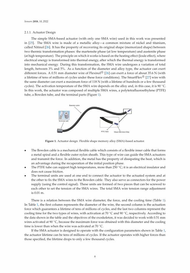
The simple SMA-based actuator (with only one SMA wire) used in this work was presentedin [25]. The SMA wire is made of a metallic alloy—a common mixture of nickel and titanium,called Nitinol [26]. It has the property of recovering its original shape (memorized shape) betweentwo thermic transformation phases: the martensite phase (at low temperature) and austenite phase(at high temperature). The principle on which it works is based on the heating effect (Joule effect), whereelectrical energy is transformed into thermal energy, after which the thermal energy is transformedinto mechanical energy. During this transformation, the SMA wire undergoes a variation of totallength, between 3% and 5%. As a function of the diameter and alloy type, the actuator can exertdifferent forces. A 0.51 mm diameter wire of Flexinol R© [26] can exert a force of about 35.6 N (witha lifetime of tens of millions of cycles under these force conditions). The SmartFlex R© [27] wire withthe same diameter can exert a maximum force of 118 N (with a lifetime of hundreds or a few thousandcycles). The activation temperature of the SMA wire depends on the alloy and, in this case, it is 90 ◦C.In this work, the actuator was composed of multiple SMA wires, a polytetrafluoroethylene (PTFE)tube, a Bowden tube, and the terminal parts (Figure 1).

Figure 1. Actuator design. Flexible shape memory alloy (SMA)-based actuator.

• The Bowden cable is a mechanical flexible cable which consists of a flexible inner cable that formsa metal spiral and a flexible outer nylon sheath. This type of wire can guide the SMA actuatorsand transmit the force. In addition, the metal has the property of dissipating the heat, which isan advantage during the recuperation of the initial position phase.

• The PTFE tube can support high temperatures, more than 250 ◦C; it is an electrical insulator anddoes not cause friction.

• The terminal units are used at one end to connect the actuator to the actuated system and atthe other to fix the SMA wires to the Bowden cable. They also serve as connectors for the powersupply (using the control signal). These units are formed of two pieces that can be screwed toeach other to set the tension of the SMA wires. The total SMA wire tension range adjustmentis 0.01 m.

There is a relation between the SMA wire diameter, the force, and the cooling time (Table 1).In Table 1, the first column represents the diameter of the wire, the second column is the actuationforce which guarantees a lifetime of tens of millions of cycles, and the last two columns represent thecooling time for the two types of wires, with activation at 70 ◦C and 90 ◦C, respectively. According tothe data shown in the table and the objectives of the exoskeleton, it was decided to work with 0.51 mmwires activated at 90 ◦C, because the maximum force was obtained with this diameter and the coolingtime is lower than when the wire was activated at 70 ◦C.

If the SMA actuator is designed to operate with the configuration parameters shown in Table 1,the actuator lifetime can be tens of millions of cycles. If the actuator operates with higher forces thanthose specified, the lifetime drops to only a few thousand cycles.

8

Sensors 2018, 18, 2522

Table 1. SMA wire characteristics [26].

Diameter Size [mm] Force [N] Cooling Time 70 ◦C [s] Cooling Time 90 ◦C [s]

0.025 0.0089 0.18 0.150.038 0.02 0.24 0.20.050 0.36 0.4 0.30.076 0.80 0.8 0.70.100 1.43 1.1 0.90.130 2.23 1.6 1.40.150 3.21 2.0 1.70.200 5.70 3.2 2.70.250 8.91 5.4 4.50.310 12.80 8.1 6.80.380 22.50 10.5 8.80.510 35.60 16.8 14.0

Regarding the application of the necessary torque to execute defined movements (the necessarytorque of each movement was found from a biomechanical simulation [3]), a summary of the systemconfiguration of the actuators can be seen in the Table 2.

Table 2. Exoskeleton actuators.

Movement SMA Wires Maximum Actuator Force [N] Length [m] Weight [kg]

Flexion 3 354 1.5 0.16Extension 2 236 1.5 0.15Pronation 1 118 2 0.1Supination 1 118 2 0.1

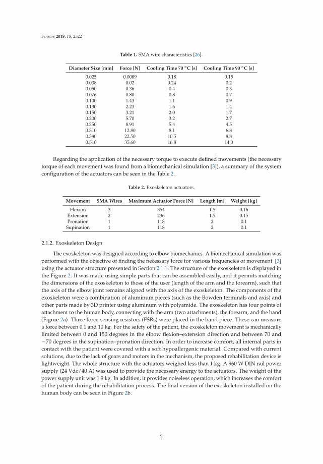
2.1.2. Exoskeleton Design

The exoskeleton was designed according to elbow biomechanics. A biomechanical simulation wasperformed with the objective of finding the necessary force for various frequencies of movement [3]using the actuator structure presented in Section 2.1.1. The structure of the exoskeleton is displayed inthe Figure 2. It was made using simple parts that can be assembled easily, and it permits matchingthe dimensions of the exoskeleton to those of the user (length of the arm and the forearm), such thatthe axis of the elbow joint remains aligned with the axis of the exoskeleton. The components of theexoskeleton were a combination of aluminum pieces (such as the Bowden terminals and axis) andother parts made by 3D printer using aluminum with polyamide. The exoskeleton has four points ofattachment to the human body, connecting with the arm (two attachments), the forearm, and the hand(Figure 2a). Three force-sensing resistors (FSRs) were placed in the hand piece. These can measurea force between 0.1 and 10 kg. For the safety of the patient, the exoskeleton movement is mechanicallylimited between 0 and 150 degrees in the elbow flexion–extension direction and between 70 and−70 degrees in the supination–pronation direction. In order to increase comfort, all internal parts incontact with the patient were covered with a soft hypoallergenic material. Compared with currentsolutions, due to the lack of gears and motors in the mechanism, the proposed rehabilitation device islightweight. The whole structure with the actuators weighed less than 1 kg. A 960 W DIN rail powersupply (24 Vdc/40 A) was used to provide the necessary energy to the actuators. The weight of thepower supply unit was 1.9 kg. In addition, it provides noiseless operation, which increases the comfortof the patient during the rehabilitation process. The final version of the exoskeleton installed on thehuman body can be seen in Figure 2b.

9

Sensors 2018, 18, 2522

(a) (b)

Figure 2. SMA exoskeleton design. (a) CAD structure: 1—attachment points with the handand force-sensing resistor (FSR) sensors, 2—fixed structure for supination–pronation, 3—actuatortermination for Bowden tube, 4—pulley for linear to rotational transformation, 5—temperature sensors,6—supination–pronation actuators, 7—flexion–extension actuators, 8—absolute encoder, 9—SMAwires. (b) SMA elbow joint exoskeleton on a human body.

2.1.3. Electronic Hardware

The electronic hardware is composed of power electronics, a controller, and sensors placed inthe device. The power electronics are capable of supplying the necessary power to four distinctactuators: flexion, extension, supination, and pronation. The system is based on a MOSFET transistor(STMicroelectronics STP310N10F7, STMicroelectronics group, Shanghai, China), which works asa switch circuit and amplifies the control signal (PWM) generated by the controller. The device wasconnected to the terminal units of the SMA-based actuator.

The controller is a 32-bit microcontroller STM32F4 from STMicroelectronics R©, China, which canbe fully programmed with Matlab/Simulink R© [28]. It was programmed with four different PWMoutput ports, which generate the necessary duty cycle for managing the four actuators (each with oneor more SMA wires).

The structure of the rehabilitation device includes sensors for position, temperature, force, andsEMG. An absolute angle position sensor with Hall effect (AS5045 made by AMS (Austrian MicroSystems), Premstaetten, Austria) is placed in the shaft of the exoskeleton (pulley for flexion–extension).This sensor has a resolution of 0.0879 degrees and measures the flexion–extension movement.The second position sensor, a membrane potentiometer made by Spectrasymbol, has a length of0.1 m and is placed on the supination–pronation piece (on the outside) to measure the absolutedisplacement of this movement. In the same piece, on the inner part which makes the connectionbetween the human forearm and hand and the exoskeleton, three FSR sensors were placed witha 60-degree angular distance between them. These sensors measure the force variation of the elbowduring flexion–extension movements—forces that are involved in the high-level control algorithm.Another main sensor involved in this algorithm is the sEMG sensor. The circuit uses three disposabledisc electrodes, F-TC1 made by SKINTACT—a low-cost, multi-purpose ECG. It consists of Ag/AgClelectrodes, a conductive gel (Aqua-Tac), an adhesive area with a dimension of 35 × 41 mm, and a snapconnection. The gel permits a better connection between the skin and the electrode. This electrode is inthe category of non-invasive and wet electrodes.

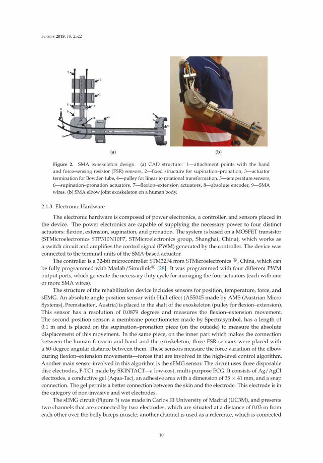
The sEMG circuit (Figure 3) was made in Carlos III University of Madrid (UC3M), and presentstwo channels that are connected by two electrodes, which are situated at a distance of 0.03 m fromeach other over the belly biceps muscle; another channel is used as a reference, which is connected

10

Sensors 2018, 18, 2522

to the last electrode positioned over the shoulder blade. The EMG circuit is composed of variousstages, including connectors. There is the differential active feedback stage, the digital stage (where thesignal is amplified and filtered), and the stage for the power supply and communication connectors.The communication between the EMG and the microcontroller uses a serial peripheral interface (SPI)bus. For the signal-processing module, we used the same microcontroller STM32F4.

Figure 3. Surface electromyography (sEMG) circuit with two channels and the electrodes: 1—electrodes,2—electrode connector, 3—connectors for power supply (5 V and GND), 4—connector for serialperipheral interface (SPI) communication.

The temperature sensors are placed in the terminal of the actuator to measure the temperature ofthe SMA wires, a parameter that is required in the control loop. All the electronics used in this projectwere based on low-cost components.

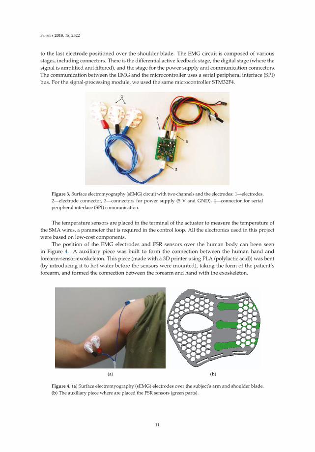
The position of the EMG electrodes and FSR sensors over the human body can been seenin Figure 4. A auxiliary piece was built to form the connection between the human hand andforearm-sensor-exoskeleton. This piece (made with a 3D printer using PLA (polylactic acid)) was bent(by introducing it to hot water before the sensors were mounted), taking the form of the patient’sforearm, and formed the connection between the forearm and hand with the exoskeleton.

(a) (b)

Figure 4. (a) Surface electromyography (sEMG) electrodes over the subject’s arm and shoulder blade.(b) The auxiliary piece where are placed the FSR sensors (green parts).

11

Sensors 2018, 18, 2522

2.2. The High-Level Control Algorithm

Previous publications [3,5] presented a low-level control algorithm based on a BPID (bilinearproportional integral derivative) controller, which governs the SMA-based exoskeleton in position.Their algorithm, involving position and temperature sensors, is capable of acquiring data from thesensors or controlling the exoskeleton in flexion, extension, or in flexion–extension using an antagonisticcontroller (two BPID controllers in a parallel configuration [5]). With the data acquisition configuration,the SMA-based exoskeleton only offers the possibility to diagnose and evaluate the patient. In thepassive mode, the actuators offer all the necessary force to reach and follow the reference positionwithout taking into account the patient force. Through the introduction of sensors for pressure/forceand sEMG, the SMA-based exoskeleton offers the possibility of rehabilitation therapies in activemode, where the reference position is generated by the patient’s movement intention. In this way,passive reference position (habitually sinusoidal movements) is changed to active reference in a casewhere the patient presents activity in the motor function (the motor function has been partiallyaffected). Active reference involves the patient undergoing rehabilitation therapy, leading to a fasterrecovery. The high-level control algorithm, which generates the active rehabilitation therapy (activereference position), uses the sEMG sensors and force-sensing resistor (FSR) sensors, together withposition sensors. This is currently available (due to the SMA-based exoskeleton configuration—in fact,the sensors) only for the elbow flexion movement.

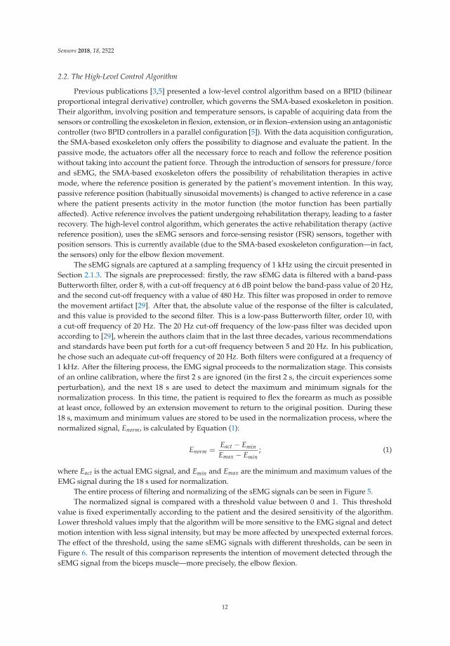
The sEMG signals are captured at a sampling frequency of 1 kHz using the circuit presented inSection 2.1.3. The signals are preprocessed: firstly, the raw sEMG data is filtered with a band-passButterworth filter, order 8, with a cut-off frequency at 6 dB point below the band-pass value of 20 Hz,and the second cut-off frequency with a value of 480 Hz. This filter was proposed in order to removethe movement artifact [29]. After that, the absolute value of the response of the filter is calculated,and this value is provided to the second filter. This is a low-pass Butterworth filter, order 10, witha cut-off frequency of 20 Hz. The 20 Hz cut-off frequency of the low-pass filter was decided uponaccording to [29], wherein the authors claim that in the last three decades, various recommendationsand standards have been put forth for a cut-off frequency between 5 and 20 Hz. In his publication,he chose such an adequate cut-off frequency of 20 Hz. Both filters were configured at a frequency of1 kHz. After the filtering process, the EMG signal proceeds to the normalization stage. This consistsof an online calibration, where the first 2 s are ignored (in the first 2 s, the circuit experiences someperturbation), and the next 18 s are used to detect the maximum and minimum signals for thenormalization process. In this time, the patient is required to flex the forearm as much as possibleat least once, followed by an extension movement to return to the original position. During these18 s, maximum and minimum values are stored to be used in the normalization process, where thenormalized signal, Enorm, is calculated by Equation (1):

Enorm =Eact − Emin

Emax − Emin; (1)

where Eact is the actual EMG signal, and Emin and Emax are the minimum and maximum values of theEMG signal during the 18 s used for normalization.

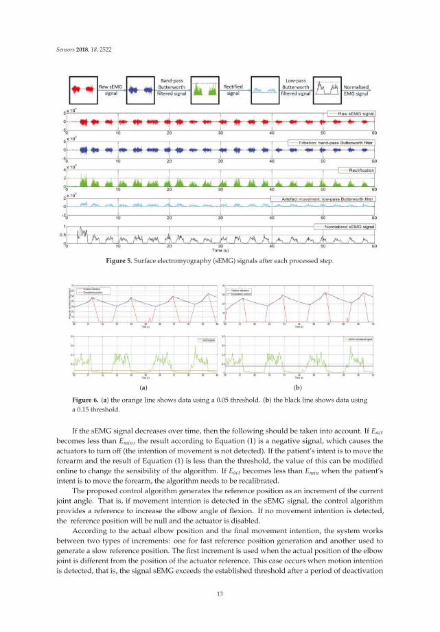
The entire process of filtering and normalizing of the sEMG signals can be seen in Figure 5.The normalized signal is compared with a threshold value between 0 and 1. This threshold

value is fixed experimentally according to the patient and the desired sensitivity of the algorithm.Lower threshold values imply that the algorithm will be more sensitive to the EMG signal and detectmotion intention with less signal intensity, but may be more affected by unexpected external forces.The effect of the threshold, using the same sEMG signals with different thresholds, can be seen inFigure 6. The result of this comparison represents the intention of movement detected through thesEMG signal from the biceps muscle—more precisely, the elbow flexion.

12

Sensors 2018, 18, 2522

Figure 5. Surface electromyography (sEMG) signals after each processed step.

(a) (b)

Figure 6. (a) the orange line shows data using a 0.05 threshold. (b) the black line shows data usinga 0.15 threshold.

If the sEMG signal decreases over time, then the following should be taken into account. If Eact

becomes less than Emin, the result according to Equation (1) is a negative signal, which causes theactuators to turn off (the intention of movement is not detected). If the patient’s intent is to move theforearm and the result of Equation (1) is less than the threshold, the value of this can be modifiedonline to change the sensibility of the algorithm. If Eact becomes less than Emin when the patient’sintent is to move the forearm, the algorithm needs to be recalibrated.

The proposed control algorithm generates the reference position as an increment of the currentjoint angle. That is, if movement intention is detected in the sEMG signal, the control algorithmprovides a reference to increase the elbow angle of flexion. If no movement intention is detected,the reference position will be null and the actuator is disabled.

According to the actual elbow position and the final movement intention, the system worksbetween two types of increments: one for fast reference position generation and another used togenerate a slow reference position. The first increment is used when the actual position of the elbowjoint is different from the position of the actuator reference. This case occurs when motion intentionis detected, that is, the signal sEMG exceeds the established threshold after a period of deactivation

13

Sensors 2018, 18, 2522

of the actuators caused by the non-detection of intention to move. The exoskeleton used in theflexion movement leaves the joint free to move, as long as the actuator is not activated because of theloss of patient motivation and engagement that results in loss of the EMG signal. At that moment,the reference position is zero, but the actual joint position is not null. This situation is shown in thedescending part of the sawtooth-shaped graph in Figure 6. The loss of intention to move producesa null reference that causes deactivation of the actuator, and the recovery of the intention causes a rapidincrease of the reference position. If the algorithm is activated and detects an intention to move, thegenerated reference uses a fast increment until it reaches the elbow position, after which it uses a slowincrement to generate the reference that will be followed by the exoskeleton, as long as there existsan intention to move. When intention to move is no longer detected, the high increment is used todecrease the reference position; the actuators are no longer activated and the extension movement iscarried out by actuator recuperation (dissipation of the heat).

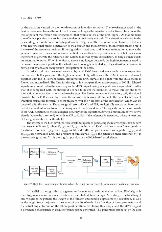
In order to address the situation caused by small EMG levels and generate the reference positionpattern with better precision, the high-level control algorithm uses the sEMG normalized signaltogether with the FSR sensor signal. Similar to the EMG signals, the signal from the FSR sensors isfiltered and normalized. The filter for this signal is a low-pass filter at a frequency of 100 Hz. Filteredsignals are normalized in the same way as the sEMG signal, using an equation analogous to (1). Afterthat, it is compared with the threshold defined to detect the intention to move through the forceinteraction between the patient and exoskeleton. For flexion movement detection, only the signalprovided by the FSR sensor placed over the radius bone is taken into account. The patient’s movementintention causes the forearm to exert pressure over the rigid part of the exoskeleton, which can bedetected with this sensor. The two signals, from sEMG and FSR, are logically compared in order todetect the final intention to move, a binary result that is used later. The logical comparison consistsof an AND function, to ensure a higher accuracy of the algorithm, having a minimum of two activesignals (above the threshold), or with an OR condition if the reference is generated, where at least oneof the signals is above the threshold.

The scheme of the high-level control algorithm capable of generating the reference position patterncan be seen in Figure 7, where Eact(k) and Pact(k) are the actual EMG and pressure or force signals inthe discrete domain, E f ilt(k) and Pf ilt(k) are filtered EMG and pressure or force signals, Enorm(k) andPnorm(k) are normalized EMG and pressure or force signals, θ(k) is the generated angle reference, V(k) isthe control signal, and Y(k) is the angular position of the SMA-based exoskeleton.

Figure 7. High-level control algorithm based on EMG and pressure signals for reference position generation.

In parallel to the algorithm that generates the reference position, the normalized EMG signal isused to generate a torque assistive reference for rehabilitation therapy. According to the total heightand weight of the patient, the weight of the forearm and hand is approximately calculated, as wellas the length from the joints to the center of gravity of each. As a function of these parameters andthe actual angle, torque on the elbow joint is estimated. Using this torque and the sEMG signal,a percentage of assistance in torque reference can be generated. This percentage can be set by the user.

14

Sensors 2018, 18, 2522

Torque assistive reference is directly proportional to the sEMG signal. A similar idea is presentedin [30], but they did not take the biomechanical structure of the human body into account.

3. Results

In order to highlight the algorithm performance, feasibility, and adaptability to various hardwareconfigurations, a series of tests were done. Firstly, simulation with EMG signals from different circuits,together with an actuator model, was conducted to simulate the behavior of the actuator in theexoskeleton; secondly, the real hardware over the exoskeleton was tested with healthy subjects.

3.1. Results of Simulation

In [31], the model of an SMA-based actuator with a variable charge was presented. This permitsthe simulation of the actuator with different SMA diameters (0.51 mm and 0.1 mm); in this case,the 0.51 mm diameter was used. According to the simulation results presented in [31], which werecompared with the real behavior of an SMA actuator, it can be concluded that the behavior of themodel is highly similar to a real actuator. To use this model in the simulation with the high-levelcontrol algorithm based on sEMG, a number of settings of the SMA-based actuator were used. Firstly,the charge of the actuator was set according to the forearm and hand weight, and the linear positionwas converted to an angular position as a function of the exoskeleton characteristics, such as the pulleyradius. It is worth noting that the SMA-based actuator model includes the same low-level controlalgorithm ([3,5]), as well as the exoskeleton.

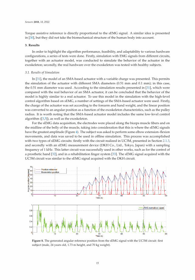
For the sEMG data acquisition, the electrodes were placed along the biceps muscle fibers and onthe midline of the belly of the muscle, taking into consideration that this is where the sEMG signalshave the greatest amplitude (Figure 4). The subject was asked to perform some elbow extension–flexionmovements, and data was saved to be used in offline simulation. This process was accomplishedwith two types of sEMG circuits: firstly with the circuit realized in UC3M, presented in Section 2.1.3,and secondly with an sEMG measurement device (DKH Co., Ltd., Tokyo, Japan) with a samplingfrequency of 1 kHz. This latter circuit was successfully used in other works, such as for the control ofa prosthetic hand [32], and in a rehabilitation finger system [33]. The sEMG signal acquired with theUC3M circuit was similar to the sEMG signal acquired with the DKH circuit.

Figure 8. The generated angular reference position from the sEMG signal with the UC3M circuit: firstsubject (male, 24 years old, 1.73 m height, and 70 kg weight).

15

Sensors 2018, 18, 2522

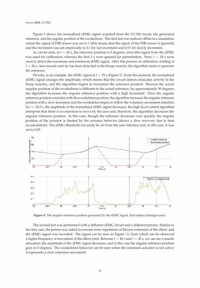
Figure 8 shows the normalized sEMG signal acquired from the UC3M circuit, the generatedreference, and the angular position of the exoskeleton. This first test was realized offline in a simulation,where the signal of FSR sensor was set to 1 (this means that the signal of the FSR sensor is ignored),and the increment was set empirically to 0.1 for fast increment and 0.01 for slowly increment.

As can be seen, at t = 20 s, the reference position is 0 degrees, since this signal from the sEMGwas used for calibration, whereas the first 2 s were ignored for perturbation. Next, t = 18 s wereused to detect the maximum and minimum sEMG signal. After this process of calibration, starting att = 20 s, once muscle activity has been detected in the biceps muscle, the algorithm starts to generatethe reference.

We take, as an example, the sEMG signal at t = 29 s (Figure 9). From this moment, the normalizedsEMG signal changes the amplitude, which means that the circuit detects muscular activity in thebicep muscles, and the algorithm begins to increment the reference position. Because the actualangular position of the exoskeleton is different to the actual reference, by approximately 30 degrees,the algorithm increases the angular reference position with a high increment. Once the angularreference position coincides with the exoskeleton position, the algorithm increases the angular referenceposition with a slow increment and the exoskeleton begins to follow the voluntary movement intention.In t = 32.5 s, the amplitude of the normalized sEMG signal decreases, the high-level control algorithminterprets that there is no intention to move by the user and, therefore, the algorithm decreases theangular reference position. In this case, though the reference decreases very quickly, the angularposition of the actuator is limited by the actuator behavior (shows a slow recovery due to heataccumulation). The sEMG threshold can easily be set from the user interface and, in this case, it wasset to 0.05.

Figure 9. The angular reference position generated by the sEMG signal, first subject (enlarged area).

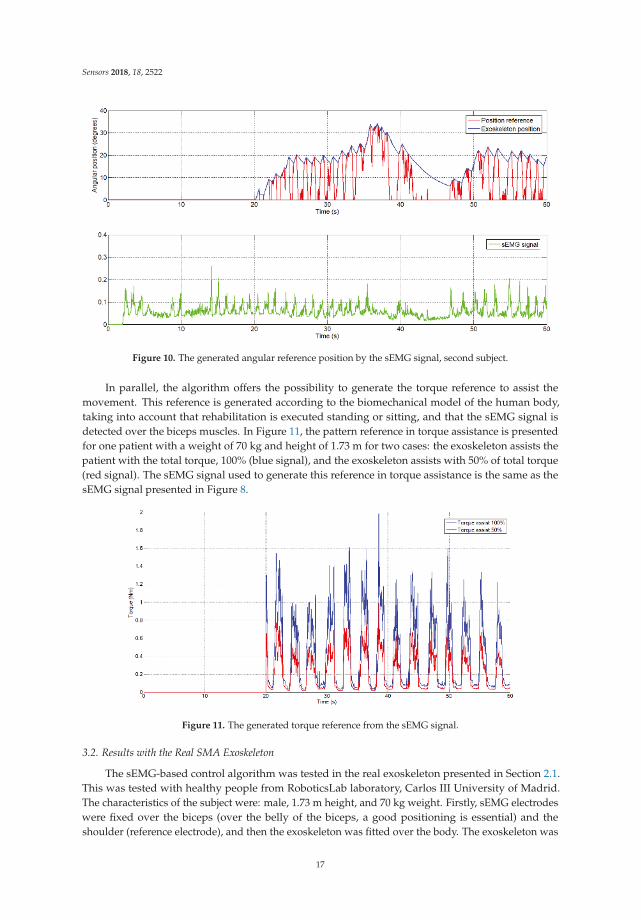
The second test was performed with a different sEMG circuit and a different person. Similar tothe first case, the person was asked to execute some repetitions of flexion–extension of the elbow andthe sEMG signal was recorded. The signal can be seen in Figure 10, from which can be observeda higher frequency of movement of the elbow joint. Between t = 40 s and t = 45 s, we can see a musclerelaxation; the amplitude of the sEMG signal decreases, and in this case the angular reference positiongoes to 0 degrees. The exoskeleton behavior can be seen when the extension actuator is not active:it represents a slow extension movement.

16

Sensors 2018, 18, 2522

Figure 10. The generated angular reference position by the sEMG signal, second subject.

In parallel, the algorithm offers the possibility to generate the torque reference to assist themovement. This reference is generated according to the biomechanical model of the human body,taking into account that rehabilitation is executed standing or sitting, and that the sEMG signal isdetected over the biceps muscles. In Figure 11, the pattern reference in torque assistance is presentedfor one patient with a weight of 70 kg and height of 1.73 m for two cases: the exoskeleton assists thepatient with the total torque, 100% (blue signal), and the exoskeleton assists with 50% of total torque(red signal). The sEMG signal used to generate this reference in torque assistance is the same as thesEMG signal presented in Figure 8.

Figure 11. The generated torque reference from the sEMG signal.

3.2. Results with the Real SMA Exoskeleton

The sEMG-based control algorithm was tested in the real exoskeleton presented in Section 2.1.This was tested with healthy people from RoboticsLab laboratory, Carlos III University of Madrid.The characteristics of the subject were: male, 1.73 m height, and 70 kg weight. Firstly, sEMG electrodeswere fixed over the biceps (over the belly of the biceps, a good positioning is essential) and theshoulder (reference electrode), and then the exoskeleton was fitted over the body. The exoskeleton was

17

Sensors 2018, 18, 2522

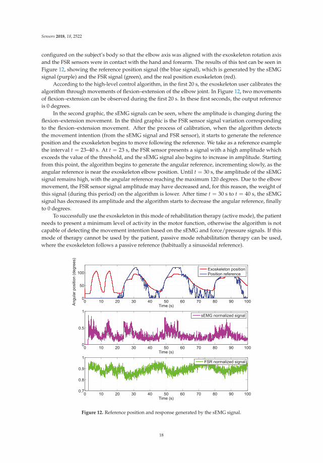
configured on the subject’s body so that the elbow axis was aligned with the exoskeleton rotation axisand the FSR sensors were in contact with the hand and forearm. The results of this test can be seen inFigure 12, showing the reference position signal (the blue signal), which is generated by the sEMGsignal (purple) and the FSR signal (green), and the real position exoskeleton (red).

According to the high-level control algorithm, in the first 20 s, the exoskeleton user calibrates thealgorithm through movements of flexion–extension of the elbow joint. In Figure 12, two movementsof flexion–extension can be observed during the first 20 s. In these first seconds, the output referenceis 0 degrees.

In the second graphic, the sEMG signals can be seen, where the amplitude is changing during theflexion–extension movement. In the third graphic is the FSR sensor signal variation correspondingto the flexion–extension movement. After the process of calibration, when the algorithm detectsthe movement intention (from the sEMG signal and FSR sensor), it starts to generate the referenceposition and the exoskeleton begins to move following the reference. We take as a reference examplethe interval t = 23–40 s. At t = 23 s, the FSR sensor presents a signal with a high amplitude whichexceeds the value of the threshold, and the sEMG signal also begins to increase in amplitude. Startingfrom this point, the algorithm begins to generate the angular reference, incrementing slowly, as theangular reference is near the exoskeleton elbow position. Until t = 30 s, the amplitude of the sEMGsignal remains high, with the angular reference reaching the maximum 120 degrees. Due to the elbowmovement, the FSR sensor signal amplitude may have decreased and, for this reason, the weight ofthis signal (during this period) on the algorithm is lower. After time t = 30 s to t = 40 s, the sEMGsignal has decreased its amplitude and the algorithm starts to decrease the angular reference, finallyto 0 degrees.

To successfully use the exoskeleton in this mode of rehabilitation therapy (active mode), the patientneeds to present a minimum level of activity in the motor function, otherwise the algorithm is notcapable of detecting the movement intention based on the sEMG and force/pressure signals. If thismode of therapy cannot be used by the patient, passive mode rehabilitation therapy can be used,where the exoskeleton follows a passive reference (habitually a sinusoidal reference).

0 10 20 30 40 50 60 70 80 90 1000

50

100

Time (s)Angu

lar p

ositi

on (d

egre

es)

Exoskeleton positionPosition reference

0 10 20 30 40 50 60 70 80 90 1000

0.5

1

Time (s)

sEMG normalized signal

0 10 20 30 40 50 60 70 80 90 1000.7

0.8

0.9

1

Time (s)

FSR normalized signal

Figure 12. Reference position and response generated by the sEMG signal.

18

Sensors 2018, 18, 2522

4. Conclusions

In this work, a new high-level control algorithm based on sEMG signals and pressure/forcesignals capable of generating the angular and torque reference for an active rehabilitation waspresented. An algorithm capable of generating the angular and torque reference was successfullytested: in simulations (with the EMG signals provided by the circuit made by the research group anda commercial circuit) and in real applications over the SMA elbow exoskeleton with healthy people.In the latter case, in a real device, the sEMG signal was used together with the force/pressure signalsfrom an FSR sensor.

The SMA-based exoskeleton for an elbow joint presented in this work, together with the low andhigh-level control algorithm and sensors, is based on low-cost components and offers three modesof operation:

• Data acquisition mode: to evaluate and diagnose the patient. Also, in this mode of operation,the angular limits of elbow movement are saved to set the angular reference limits for thecontrol algorithm.

• Passive rehabilitation mode: The exoskeleton follows a defined angular reference, the mostcommon being a sinusoidal type. In this case, the patient executes repetitive movements, nottaking into account the movement intention of the patient. The exoskeleton can support all themovement in flexion, extension, or flexion–extension.

• Active rehabilitation mode: The angular reference for the elbow exoskeleton is generatedas a function of the patient’s intention for movement, detected by the sEMG signals andforce/pressure signals. In this case, the patient is actively involved in the rehabilitation therapy,and if movement intention is not detected, the angular reference goes to 0 degrees. This type ofrehabilitation can only be used with patients who present a minimum activity level in their motorfunction; otherwise, a passive rehabilitation can be used.

The performance of the high-level control algorithm considered the biceps muscle activity anddid not take into account the triceps muscle activity. If this co-contraction appears, and the FSR sensoris not capable of detecting it, the user needs to manually stop the system.

The control algorithm presented in this paper permits the adjustment of the parameters of thegenerated reference position, such as the increments (which modify the angular velocity response ofthe exoskeleton) and the thresholds of the sEMG and FSR signals, which change the sensibility of thealgorithm (from which signal value the algorithm starts to increment to the reference position).

The main advantage provided by the proposed high-level controller is that it forces the patient tobe involved in the therapy task on a constant basis. If the patient loses attention, the exoskeleton isdeactivated. In this way, the controller promotes active rehabilitation.

Author Contributions: L.M. was in charge of project administration and funding acquisition. D.C. and L.M.designed the exoskeleton. D.C. developed the control method and carried out the experiments. D.S. collaboratedin experiments. D.B. supervised the research. D.C. and D.B. wrote the manuscript.

Funding: The research was funded by RoboHealth (DPI2013-47944-C4-3-R) and the EDAM(DPI2016-75346-R) Spanish research projects.

Acknowledgments: The authors are grateful for the collaboration of the LAMBECOM research group, of ReyJuan Carlos University of Madrid, Spain, in defining the design requirements of the rehabilitation device and theirparticipation in the evaluation of preliminary designs.

Conflicts of Interest: The authors declare no conflict of interest.

19

Sensors 2018, 18, 2522

Abbreviations

The following abbreviations are used in this manuscript:

SMA Shape Memory AlloyUC3M Carlos III University of MadridFSR Force Sensing ResistorPWM Pulse-Width ModulationsEMG Surface electromyographyPTFE PolytetrafluoroethyleneDOF Degrees of freedomSPI Serial Peripheral InterfacePLA Polylactic AcidMES Myoelectric signals

References

1. Harwin, W.S.; Murgia, A.; Stokes, E.K. Assessing the effectiveness of robot facilitates neurorehabilitation forrelearning motor skills. Med. Biol. Eng. Comput. 2011, 49, 1093–1102. [CrossRef] [PubMed]

2. Pons, J.L. Wearable Robots; John Wiley & Sons: Chichester, UK, 2008.3. Copaci, D.; Flores, A.; Rueda, F.; Alguacil, I.; Blanco, D.; Moreno, L. Wearable Elbow Exoskeleton Actuated

with Shape Memory Alloy. In Converging Clinical and Engineering Research on Neurorehabilitation II, Proceedings

of the 3rd International Conference on NeuroRehabilitation (ICNR2016) Segovia, Spain, 18–21 October 2016;Springer: Basel, Switzerland, 2016; pp. 477–481.

4. Copaci, D. Non-Linear Actuators and Simulation Tools for Rehabilitation Devices. Ph.D. Thesis, Carlos IIIUniversity, Getafe, Spain, 2017.

5. Copaci, D.; Blanco, D.; Moreno, L. Wearable elbow exoskeleton actuated with Shape Memory Alloy inantagonist movement. In Proceedings of the Joint Workshop on Wearable Robotics and Assistive Devices,International Conference on Intelligent Robots and Systems (IROS 2016), Daejeon, Korea, 9–14 October 2016.

6. Norman, R.W.; Komi, P.V. Electromechanical delay in skeletal muscle under normal movement conditions.Acta Physiol. Scand. 1979, 106, 241–248. [CrossRef] [PubMed]

7. DiCicco, M.; Lucas, L.; Matsuoka, Y. Comparison of Two Control Strategies for a Muscle Controlled OrthoticExoskeleton for the Hand. In Proceedings of the IEEE International Conference on Robotics and Automation,New Orleans, LA, USA, 26 April–1 May 2004; pp. 1622–1627.

8. Martini, F.H.; Timmons, M.J.; Tallitsch, R.B. Human Anatomy; Pearson Education Inc.: Old Tappan, NJ, USA,1997; ISBN 0-13-049178-0.

9. Battye, C.K.; Nightingale, A.; Whillis, J. The use of myo-electric currents in the operation of prostheses.Bone Jt. J. 1955, 37, 506–510. [CrossRef]

10. Bottomley, A.H. Myo-electric control of powered prostheses. Bone Jt. J. 1965, 47, 411–415. [CrossRef]11. Farry, K.A.; Walker, L.D.; Baraniuk, R.B. Myoelectric Teleoperation of a Complex Robotic Hand. IEEE Trans.

Rob. Autom. 1996, 12, 775–788. [CrossRef]12. Fukuda, O.; Tsuji, T.; Ohtsuka, A.; Kaneko, M. EMG-based Human-Robot Interface for Rehabilitation

Aid. In Proceedings of the IEEE International Conference on Robotics and Automation, Leuven, Belgium,16–20 May 1998; pp. 3942–3947.

13. Kuribayashi, K.; Shimizu, S.; Okimura, K.; Taniguchi, T. A discrimination system using neuralnetwok for EMG-control prostheses-Integral type of emg signal processing. In Proceedings of the 1993IEEERSJ International Conference on Intelligent Robots and Systems, Yokohama, Japan, 26–30 July 1993;pp. 1750–1755.

14. Benjnya, N.; Kenney, S.B. Myoelectric Hand Orthosis. J. Prosthet. Orthot. 1990, 2, 149–154.15. Singh, R.M.; Chatterji, S. Trends and Callenges in EMG Based Control Scheme of Exoskeleton

Robots—A Review. Int. J. Sci. Eng. Res. 2012, 3, 506–510.16. Vasan, G.; Pilarski, P. Learning from Demonstration: Teaching a Myoelectric Prosthesis with an Intact Limb

via Reinforcement Learning. In Proceedings of the 15th International Conference on Rehabilitation Robotics(ICORR2017), London, UK, 17–20 July 2017.

20

Sensors 2018, 18, 2522

17. Hudgins, B.; Parker, P.; Scott, R. A new strategy for multifunction myoelectric control. IEEE Trans.

Biomed. Eng. 1993, 40, 82–94. [CrossRef] [PubMed]18. Au, A.T.C.; Kirsch, R.F. EMG-based prediction of shoulder and elbow kinematics in able-bodied and spinal

cord injured individuals. IEEE Trans. Rehabil. Eng. 2000, 8, 471–480. [CrossRef] [PubMed]19. Kiguchi, K.; Tanaka, T.; Fukuda, T. Neuro-Fuzzy Control of a Robotic Exoskeleton with EMG Signals.

IEEE Trans. Fuzzy Syst. 2004, 12, 481–490. [CrossRef]20. Gopura, R.; Kiguchi, K. An Exoskeleton Robot for Human Forearm and Wrist Motion Assist-Hardware

Design and EMG-Based Controller. Int. J. Adv. Mech. Des. Syst. Manuf. 2008, 2, 1067–1083.21. Gopura, R.; Kiguchi, K. Application of Surface Electromyographic Signals to Control Exoskeleton Robots.

In Applications of EMG in Clinical and Sports Medicine Catriona Steele; IntechOpen: Rijeka, Croatia, 2012.22. Kiguchi, K.; Hayashi, Y. An EMG-Based Control for an Upper-Limb Power-Assist Exoskeleton Robot.

IEEE Trans. Syst. Man Cybern. Part B Cybern. 2012, 42, 1064–1071. [CrossRef] [PubMed]23. Lenzi, T.; de Rossi, S.M.M.; Vitiello, N.; Carroza, M.C. Intention-Based EMG Control of Powered Exoskeletons.

IEEE Trans. Biomed. Eng. 2012, 58, 2180–2190. [CrossRef] [PubMed]24. Lucas, L.; DiCicco, M.; Matsuoka, Y. An EMG-Controlled Hand Exoskeleton for Natural Pinching.

J. Robot. Mechatron. 2004, 16, 482–488. [CrossRef]25. Villoslada, A.; Flores, A.; Copaci, D.; Blanco, D.; Moreno, L. High displacement flexible shape memory alloy

actuator for soft wearable robots. Robot. Auton. Syst. 2015, 73, 91–101. [CrossRef]26. Technical Characteristics of Flexinol, Dynalloy, Inc. Makers of Dynamic Alloys. Available online:

http://www.dynalloy.com/ (accessed on 18 June 2018).27. Saes Group. Available online: https://www.saesgetters.com/ (accessed on 18 June 2018).28. Flores, A.; Copaci, D.; Villoslada, A.; Blanco, D.; Moreno, L. Sistema Avanzado de Protipado Rápido para

Control en la Educación en Ingeniería para grupos Multidisciplinares. Rev. Iberoam. Autom. Inf. Ind. 2016, 13,350–362.

29. De Luca, C.J.; Gilmore, L.D.; Kuznetsov, M.; Roy, S.H. Filtering the surface EMG signal: Movement artifactand baseline noise contamination. J. Biomech. 2010, 43, 1573–1579. [CrossRef] [PubMed]

30. Song, R.; Tong, K.Y.; Hu, X.; Li, L. Assistive Control System Using Continuous Myoelectric Signal inRobot-Aided Arm Training for Patients after Stroke. IEEE Trans. Neural Syst. Rehabil. Eng. 2008, 16, 371–379.[CrossRef] [PubMed]

31. Copaci, D.; Flores, A.; Villoslada, A.; Blanco, D. Modelado y Simulación de Actuadores SMA con CargaVariable. In Proceedings of the XXXVI Jornadas de Automática, Bilbao, Spain, 2–4 September 2015.

32. Hioki, M.; Ebisawa, S.; Sakaeda, H.; Mouri, T.; Nakagawa, S.; Uchida, Y.; Kawasaki, H. Design andcontrol of electromyogram prosthetic hand with high grasping force. In Proceedings of the 2011 IEEEInternational Conference on Robotics and Biomimetics, Karon Beach, Phuket, Thailand, 7–11 December 2011;pp. 1128–1133.

33. Hioki, M.; Kawasaki, H.; Sakaeda, H.; Nishimoto, Y.; Mouri, T. Finger Rehabilitation Support System Usinga Multifingered Haptic Interface Controlled by a Surface Electromyogram. J. Robot. 2011, 167516. [CrossRef][PubMed]

c© 2018 by the authors. Licensee MDPI, Basel, Switzerland. This article is an open accessarticle distributed under the terms and conditions of the Creative Commons Attribution(CC BY) license (http://creativecommons.org/licenses/by/4.0/).

21

sensors

Article

Intelligent Multimodal Framework for HumanAssistive Robotics Based on ComputerVision Algorithms

Eugenio Ivorra 1,*, Mario Ortega 1, José M. Catalán 2,*, Santiago Ezquerro 2, Luis Daniel Lledó 2,

Nicolás Garcia-Aracil 2 and Mariano Alcañiz 1

1 Institute for Research and Innovation in Bioengineering, Universitat Politècnica de València,46022 Valencia, Spain; mortega@i3b.upv.es (M.O.); malcaniz@i3b.upv.es (M.A.)

2 Biomedical Neuroengineering Group, Universidad Miguel Hernández de Elche, 03202 Elche, Spain;sezquerro@umh.es (S.E.); llledo@umh.es (L.D.L.); nicolas.garcia@umh.es (N.G.-A.)

* Correspondence: euivmar@i3b.upv.es or euivmar@upvnet.upv.es (E.I.); jcatalan@umh.es (J.M.C.)

Received: 4 July 2018; Accepted: 23 July 2018; Published: 24 July 2018

Abstract: Assistive technologies help all persons with disabilities to improve their accessibility inall aspects of their life. The AIDE European project contributes to the improvement of currentassistive technologies by developing and testing a modular and adaptive multimodal interfacecustomizable to the individual needs of people with disabilities. This paper describes the computervision algorithms part of the multimodal interface developed inside the AIDE European project.The main contribution of this computer vision part is the integration with the robotic system andwith the other sensory systems (electrooculography (EOG) and electroencephalography (EEG)).The technical achievements solved herein are the algorithm for the selection of objects using thegaze, and especially the state-of-the-art algorithm for the efficient detection and pose estimation oftextureless objects. These algorithms were tested in real conditions, and were thoroughly evaluatedboth qualitatively and quantitatively. The experimental results of the object selection algorithm wereexcellent (object selection over 90%) in less than 12 s. The detection and pose estimation algorithmsevaluated using the LINEMOD database were similar to the state-of-the-art method, and were themost computationally efficient.

Keywords: 3D object detection and pose estimation; assistive robotics; eye-tracking;human–computer interface

1. Introduction

Approximately 80 million people in the European Union (one-sixth of its population) havea disability. The percentage of people with disabilities is set to rise as the EU population ages [1].

Accessibility is a basic right for all persons with disabilities according to Article 9 of theUnited Nations Convention on the Rights of Persons with Disabilities. The purpose of accessibilityis to enable persons with disabilities to live independently and to participate in all aspects of life.Assistive technologies help all persons with disabilities to improve their accessibility in all aspectsof their life. Current trends in assistive technology for supporting activities of daily living (ADL),mobility, communication, and so on are based on the integration of the capabilities of the user andthe assistive technologies. The improvement of the interaction and cooperation between the user andthe assistive technologies can be split into three main areas: (1) improvements of the assistive devices,such as mechanical parts, electronic parts, etc.; (2) improvements of the user–technology interface;and (3) improved shared control between the user and the assistive technology. The AIDE Europeanproject contributes to improving current assistive technologies by developing and testing a modular

Sensors 2018, 18, 2408; doi:10.3390/s18082408 www.mdpi.com/journal/sensors22

Sensors 2018, 18, 2408

and adaptive multimodal interface customizable to the individual needs of people with disabilities aswell as a totally new shared control paradigm for assistive devices that integrates information from theidentification of the residual abilities, behaviours, emotional state, and intentions of the user on onehand and the analysis of the environment through the use of cameras and context factors on the other.This paper describes the computer vision algorithms part of the multimodal interface developed withinthe AIDE European project.

There are some examples of multi-modal architectures for the interaction and control of assistiverobotic devices. Specifically, Meng et al. presented a non-invasive brain–computer interface (BCI) forcontrolling a robotic arm to complete reach-and-grasp tasks [2]. They used a Microsoft Kinect MotionSensor to locate and send the position of a target to the robot control system. Another interestingrecent paper presented an assisted feeding strategy that uses a Kinect camera and a modular roboticarm to implement a closed-form system that performs assisted feeding [3]. In contrast to these works,our approach uses two cameras (one looking at the environment in front of the user and the otherlooking at the user) to locate real objects and the user’s mouth position, respectively. In addition, theuser wears a pair of eye-tracking glasses to recognise the object at which the user is looking. There arealso some works using invasive BCI systems in people with long-standing tetraplegia to control arobotic arm to perform three-dimensional reach and grasp movements [4,5]. Some works can befound in the literature reporting the control of an arm exoskeleton using multimodal interfaces.Specifically, Pedrocchi et al. developed a novel system composed of a passive arm exoskeleton,a robotic hand orthesis, and a neuromuscular electrical stimulation system driven by residualvoluntary muscular activation, head/eye motion, and brain signals in the framework of the MUNDUSproject [6]. In addition, Frisoli et al. presented a robotic-assisted rehabilitation training with an upperlimb robotic exoskeleton for the restoration of motor function in spatial reaching movements [7].Then, they presented the multimodal control of an arm–hand robotic exoskeleton to perform activitiesof daily living. The presented system was driven by a shared control architecture using BCI andeye gaze tracking for the control of an arm exoskeleton and a hand exoskeleton for reaching andgrasping/releasing cylindrical objects of different size in the framework of the BRAVO project [8].Most recently, Clemente et al. presented a motion planning system based on learning by demonstrationfor upper-limb exoskeletons that allow the successful assistance of patients during activities of dailyliving (ADL) in an unstructured environment using a multimodal interface, while ensuring thatanthropomorphic criteria are satisfied in the whole human–robot workspace [9]. In contrast to theprevious works, the AIDE multimodal control interface predicts the activity that the user wants toperform and allows the user to trigger the execution of different sub-actions that compose the predictedactivity, and to interrupt the task at any time by means of the hybrid control interface based on asystem combining gaze tracking, electroencephalography (EEG), and electrooculography (EOG).

Most activities of daily living require complete reach-and-grasp tasks. The grasping task is acommon operation for fixed manipulators in a controlled environment, but assistive robotics have thecomplexity that this environment is not fixed. Moreover, it should be solved in real-time in order to becomfortable for humans and sufficiently precise to perform successful grasps of a variety of objects.To sum up, a grasping task in multimodal assistive robotics requires the processing of a preciselocation and orientation of common textureless objects in real-time. Some authors have solved itusing commercial tracking systems like Optitrack© or ART Track© [10–12], but these solutions requirethe modification of the objects by adding specific marks. Our proposal employs a computer visionapproach that does not have that limitation. There are multiple technical approaches to solving thisproblem, and despite the great advances made recently in the field of computer vision (especiallywith the new deep learning techniques), it is still a difficult problem to solve effectively—specificallywhen the 3D object is textureless. For well-textured objects, several methods based on appearancedescriptors like SURF or SIFT [13] can be employed to solve this problem. However, most commonobjects in our context (home) are textureless.

23

Sensors 2018, 18, 2408

Considering the technical features required, these methods should be efficient, accurate, scalable,and robust to changes in the environment (no controlled light conditions or occlusions).

The main lines of investigation in the field of 3D textureless object pose estimation are methodsbased on geometric 3D descriptors, template matching, deep learning techniques, and random forests.

Methods based on geometric 3D descriptors employ the information extracted from the geometry ofthe 3D models of the objects. There are two kinds of 3D descriptors: local descriptors and global descriptors.

On one hand, local descriptors are obtained from characteristic local geometric points fromthe model. Once descriptors are calculated from the model and from the depth image from the RGB-Dcamera, a matching correspondence can be obtained. The last stage is usually a refinement of the poseusing an iterative closest point algorithm (ICP [14] Among these methods [15] stand out FPFH [16],PPF [17], and SHOT [18]. These methods are very computationally expensive (need several secondsfor estimating the object pose), but are robust to occlusions. One of the most employed methodsis the point pair features (PPFs). This method was developed by Drost et al. [17] and employs thedepth image for estimating local descriptors using normals of the object. Later, several authors haveoptimised the original implementation, greatly reducing the computational cost of the algorithm(Stefan et al. [19] still requires between 0.1 and 0.8 s for processing an image). However, the algorithmis still too heavy for real-time use.

On the other hand, global descriptors encode the shape of the 3D model in a single vector.The main global descriptor classes are VFH [20], OUR-CVFH [21], and ESF [22]. In contrast to thelocal descriptors, and as the main disadvantages, it is necessary to first have the 3D reconstruction ofthe object, as well as to segment the scene before estimating the pose of the object. In addition, thesemethods are very sensitive to the occlusion of the object. On the other hand and as a main advantage,they are computationally efficient. These types of descriptors are usually used for their efficiencyin problems of classification or 3D model retrieval. In addition, note that these geometric methods(both local and global descriptors) can also use the colour information of the object (if it is available),increasing the robustness of the method (e.g., the local descriptor CSHOT [23]).

Methods based on template matching efficiently search through the generated set of templates ofa 3D model employing a sliding window approach to find the most similar template within an image,as well as its 2D location using a similarity criterion. Once the most similar template is determinedwithin the image, the initial pose of the 3D object is inferred from the one associated with the template.Within these methods, the algorithm LINEMOD++ [24] stands out. This algorithm is one of themost-employed algorithms by the scientific community for estimating the pose due to its high efficiencyand robustness. Specifically, Hinterstoisser et al. [24] were the first to use this LINEMOD detectionmethod to estimate the pose of objects. The LINEMOD method uses the information extracted from thegradients of a colour image and the surface normals. This information is subsequently quantified so thatthe search for the most similar template is carried out efficiently. Then, Hinterstoisser et al. [24] addeda post-process stage in order to strengthen the detection method by eliminating some of the possiblefalse positives. The last stage is a refinement of the pose using an ICP algorithm. This implementationwas enhanced by Kehl et al. [25] to increase its scalability.

Another similar template method was proposed by Hodan et al. [26]. Unlike the original LINEMOD++method, they initially limit the search to certain areas of the image, by means of a simple filteringtechnique. The matching between the templates and the remaining possible locations within theimage is done with a voting procedure based on hashing. To refine the pose, they use particle swarmoptimization (PSO) [26] in place of the ICP algorithm. Following the same line, Zhang et al. [27]proposes that in addition the detection method be invariant to scale, consequently reducing the numberof templates on which to perform the search. Despite all these modifications, these methods [25–27] areless precise and more computationally expensive than the LINEMOD++ method. The main limitationof methods based on templates is that they are very sensitive to object occlusion. On the contrary, theyare usually computationally efficient methods when compared with methods based on 3D descriptorsor deep learning techniques.

24

Sensors 2018, 18, 2408

Recently, multiple methods have appeared that address the problem of estimating the pose ofa 3D object through the use of deep learning techniques. Among the most popular methods are theSSD-6D [28], BB8 [29], Pose-CNN [30], and [31,32] methods. The main advantages of these methodsare that they allow estimation of the pose using only the RGB sensor information, the scalability, andthe robustness against occlusion. However, and as one of the main disadvantages, most of thesemethods need a large amount of training images to detect and estimate the pose of an object. Moreover,there is the added difficulty of estimating the actual pose associated with the training images. Thissupposes a great effort and time of work on the part of the user, as much the compilation of images ofthe 3D model as the estimation of the pose in each of them. To solve this type of limitation, methodssuch as the SSD-6D [28] method have been used to estimate the pose of objects using deep learningtechniques using only synthetic images extracted from the original 3D model. However, these methodscan have problems when there are substantial differences between the appearance of the syntheticimages of the 3D model and the appearance of the images captured by the camera [28] (e.g., localchanges in the illumination due to specular reflections). In turn, simply the change in the specificationsof the capture sensor in the test phase can substantially influence the results [33]. To mitigate thisproblem, it is necessary to obtain 3D models of 3D objects with photorealistic quality. Although thesemethods present promising results, the 3D models of the objects must have colour information sothat the pose can be detected and estimated correctly. This is a problem because it is common to onlyhave access to a CAD model of the object without colour, or models are obtained through the use of adepth camera/RGB-D and KinectFusion technology [34], resulting in non-photorealistic models. It isimportand to remark that training these models requires high-end equipment and/or a lot of time oncethe training information is ready. On the other hand, except for the SSD-6D [28] method that works at10 fps, these are very computationally expensive, preventing their use in real-time. In addition, allthese methods need a high-performance GPU.

Finally, the last types of methods are those based on forest classifiers. Some examples of thesemethods are those proposed by Brachmann et al. [35,36] in which they predict the 3D coordinates ofan object as well as the labels assigned to each class by means of a random forest. Then, they use theRANSAC algorithm to estimate the initial pose. This method is very robust to the occlusion problem.Another outstanding work is the method of Tejani et al. [37]. They use the “latent-class Hough forest”method with the extracted information (features) of the LINEMOD algorithm on RGB-D patches toestimate the pose of the object. This method is invariant to scale and also allows estimation of the poseof multiple instances of the same 3D object.

In summary, this paper presents the computer vision algorithms developed in the AIDEmulti-modal architecture for human assistive robotics that is able to give accessibility to personswith disabilities. The main contribution of this computer vision component is the integration withthe robotic system and with the other sensory systems (EOG and EEG). The technical achievementssolved are the algorithm for the selection of objects using the gaze and especially the state-of-the-artalgorithm for the efficient detection and pose estimation of textureless objects. These algorithmswere tested in real conditions with patients, and were also thoroughly evaluated both qualitativelyand quantitatively. This paper is organised as follows. Section 2 presents the experimental setup withthe multi-modal interface composition, the integration with the robotic system, and the developedcomputer vision algorithms. Section 3 shows quantitative and qualitative experimental results toevaluate the computer vision algorithm, and finally, Section 4 presents the conclusions and the futurework planned.

2. Materials and Methods

2.1. Experimental Section

All participants were sitting in an electric wheelchair in front of a desk. Moreover, a Jaco2 robot isattached to the wheelchair (see Figure 1). In addition, the multimodal interface is composed of: (1) a pair

25

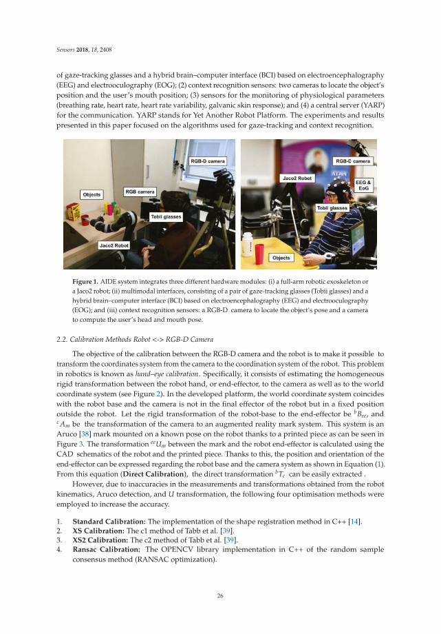
Sensors 2018, 18, 2408

of gaze-tracking glasses and a hybrid brain–computer interface (BCI) based on electroencephalography(EEG) and electrooculography (EOG); (2) context recognition sensors: two cameras to locate the object’sposition and the user’s mouth position; (3) sensors for the monitoring of physiological parameters(breathing rate, heart rate, heart rate variability, galvanic skin response); and (4) a central server (YARP)for the communication. YARP stands for Yet Another Robot Platform. The experiments and resultspresented in this paper focused on the algorithms used for gaze-tracking and context recognition.

Figure 1. AIDE system integrates three different hardware modules: (i) a full-arm robotic exoskeleton ora Jaco2 robot; (ii) multimodal interfaces, consisting of a pair of gaze-tracking glasses (Tobii glasses) and ahybrid brain–computer interface (BCI) based on electroencephalography (EEG) and electrooculography(EOG); and (iii) context recognition sensors: a RGB-D camera to locate the object’s pose and a camerato compute the user’s head and mouth pose.

2.2. Calibration Methods Robot <-> RGB-D Camera

The objective of the calibration between the RGB-D camera and the robot is to make it possible totransform the coordinates system from the camera to the coordination system of the robot. This problemin robotics is known as hand–eye calibration. Specifically, it consists of estimating the homogeneousrigid transformation between the robot hand, or end-effector, to the camera as well as to the worldcoordinate system (see Figure 2). In the developed platform, the world coordinate system coincideswith the robot base and the camera is not in the final effector of the robot but in a fixed positionoutside the robot. Let the rigid transformation of the robot-base to the end-effector be bBee, andc Am be the transformation of the camera to an augmented reality mark system. This system is anAruco [38] mark mounted on a known pose on the robot thanks to a printed piece as can be seen inFigure 3. The transformation eeUm between the mark and the robot end-effector is calculated using theCAD schematics of the robot and the printed piece. Thanks to this, the position and orientation of theend-effector can be expressed regarding the robot base and the camera system as shown in Equation (1).From this equation (Direct Calibration), the direct transformation bTc can be easily extracted .

However, due to inaccuracies in the measurements and transformations obtained from the robotkinematics, Aruco detection, and U transformation, the following four optimisation methods wereemployed to increase the accuracy.

1. Standard Calibration: The implementation of the shape registration method in C++ [14].2. XS Calibration: The c1 method of Tabb et al. [39].3. XS2 Calibration: The c2 method of Tabb et al. [39].4. Ransac Calibration: The OPENCV library implementation in C++ of the random sample

consensus method (RANSAC optimization).

26

Sensors 2018, 18, 2408

Figure 2. Schematic of the robot—camera problem.

Figure 3. Calibration program.

Methods 1 and 4 employ the strategy of estimating the transformation between a cloud of 3Dpoints expressed in the robot base and a cloud of the same points expressed in the camera system.Methods 2 and 3 were developed by Tabb et al. [39], and are based on the homogeneous matrix equationAX = ZB where Z is the transformation from camera to robot base and X is the transformation fromrobot base to world coordinate. The difference between both methods is the cost function employedfor the optimisation of transformations, as shown in Equations (2) and (3), respectively.

(bBee ←→c Am ∗m Uee) (1)

c1 =i=0

∑n−1

||AiX − ZBi||2F (2)

c2 =i=0

∑n−1

∣∣∣∣∣∣Ai − ZBiX

−1∣∣∣∣∣∣2

F(3)

27

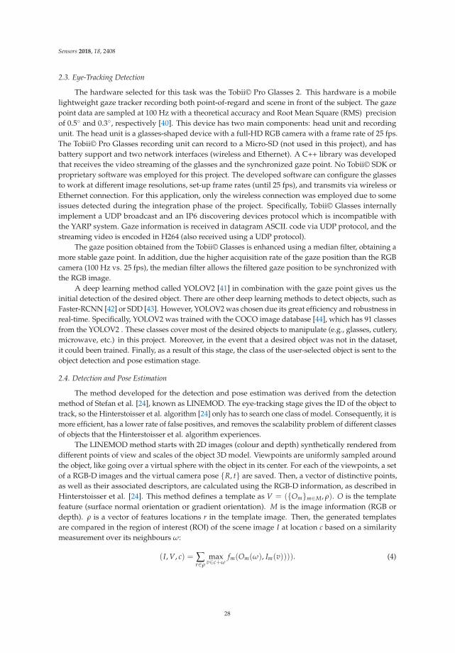
Sensors 2018, 18, 2408

2.3. Eye-Tracking Detection

The hardware selected for this task was the Tobii© Pro Glasses 2. This hardware is a mobilelightweight gaze tracker recording both point-of-regard and scene in front of the subject. The gazepoint data are sampled at 100 Hz with a theoretical accuracy and Root Mean Square (RMS) precisionof 0.5◦ and 0.3◦, respectively [40]. This device has two main components: head unit and recordingunit. The head unit is a glasses-shaped device with a full-HD RGB camera with a frame rate of 25 fps.The Tobii© Pro Glasses recording unit can record to a Micro-SD (not used in this project), and hasbattery support and two network interfaces (wireless and Ethernet). A C++ library was developedthat receives the video streaming of the glasses and the synchronized gaze point. No Tobii© SDK orproprietary software was employed for this project. The developed software can configure the glassesto work at different image resolutions, set-up frame rates (until 25 fps), and transmits via wireless orEthernet connection. For this application, only the wireless connection was employed due to someissues detected during the integration phase of the project. Specifically, Tobii© Glasses internallyimplement a UDP broadcast and an IP6 discovering devices protocol which is incompatible withthe YARP system. Gaze information is received in datagram ASCII. code via UDP protocol, and thestreaming video is encoded in H264 (also received using a UDP protocol).

The gaze position obtained from the Tobii© Glasses is enhanced using a median filter, obtaining amore stable gaze point. In addition, due the higher acquisition rate of the gaze position than the RGBcamera (100 Hz vs. 25 fps), the median filter allows the filtered gaze position to be synchronized withthe RGB image.

A deep learning method called YOLOV2 [41] in combination with the gaze point gives us theinitial detection of the desired object. There are other deep learning methods to detect objects, such asFaster-RCNN [42] or SDD [43]. However, YOLOV2 was chosen due its great efficiency and robustness inreal-time. Specifically, YOLOV2 was trained with the COCO image database [44], which has 91 classesfrom the YOLOV2 . These classes cover most of the desired objects to manipulate (e.g., glasses, cutlery,microwave, etc.) in this project. Moreover, in the event that a desired object was not in the dataset,it could been trained. Finally, as a result of this stage, the class of the user-selected object is sent to theobject detection and pose estimation stage.

2.4. Detection and Pose Estimation

The method developed for the detection and pose estimation was derived from the detectionmethod of Stefan et al. [24], known as LINEMOD. The eye-tracking stage gives the ID of the object totrack, so the Hinterstoisser et al. algorithm [24] only has to search one class of model. Consequently, it ismore efficient, has a lower rate of false positives, and removes the scalability problem of different classesof objects that the Hinterstoisser et al. algorithm experiences.

The LINEMOD method starts with 2D images (colour and depth) synthetically rendered fromdifferent points of view and scales of the object 3D model. Viewpoints are uniformly sampled aroundthe object, like going over a virtual sphere with the object in its center. For each of the viewpoints, a setof a RGB-D images and the virtual camera pose {R, t} are saved. Then, a vector of distinctive points,as well as their associated descriptors, are calculated using the RGB-D information, as described inHinterstoisser et al. [24]. This method defines a template as V = ({Om}m∈M, ρ). O is the templatefeature (surface normal orientation or gradient orientation). M is the image information (RGB ordepth). ρ is a vector of features locations r in the template image. Then, the generated templatesare compared in the region of interest (ROI) of the scene image I at location c based on a similaritymeasurement over its neighbours ω:

(I, V, c) = ∑r∈ρ

maxv∈c+ω

fm(Om(ω), Im(v)))). (4)

28

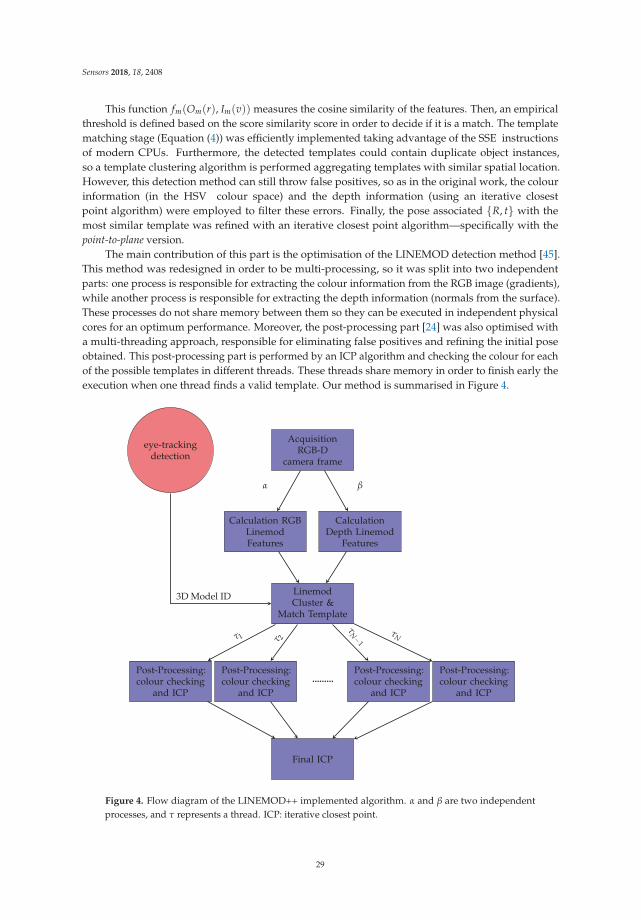
Sensors 2018, 18, 2408

This function fm(Om(r), Im(v)) measures the cosine similarity of the features. Then, an empiricalthreshold is defined based on the score similarity score in order to decide if it is a match. The templatematching stage (Equation (4)) was efficiently implemented taking advantage of the SSE instructionsof modern CPUs. Furthermore, the detected templates could contain duplicate object instances,so a template clustering algorithm is performed aggregating templates with similar spatial location.However, this detection method can still throw false positives, so as in the original work, the colourinformation (in the HSV colour space) and the depth information (using an iterative closestpoint algorithm) were employed to filter these errors. Finally, the pose associated {R, t} with themost similar template was refined with an iterative closest point algorithm—specifically with thepoint-to-plane version.

The main contribution of this part is the optimisation of the LINEMOD detection method [45].This method was redesigned in order to be multi-processing, so it was split into two independentparts: one process is responsible for extracting the colour information from the RGB image (gradients),while another process is responsible for extracting the depth information (normals from the surface).These processes do not share memory between them so they can be executed in independent physicalcores for an optimum performance. Moreover, the post-processing part [24] was also optimised witha multi-threading approach, responsible for eliminating false positives and refining the initial poseobtained. This post-processing part is performed by an ICP algorithm and checking the colour for eachof the possible templates in different threads. These threads share memory in order to finish early theexecution when one thread finds a valid template. Our method is summarised in Figure 4.

AcquisitionRGB-D

camera frame

eye-trackingdetection

Calculation RGBLinemodFeatures

CalculationDepth Linemod

Features

LinemodCluster &

Match Template

Post-Processing:colour checking

and ICP

Post-Processing:colour checking

and ICP.........

Post-Processing:colour checking

and ICP

Post-Processing:colour checking

and ICP

Final ICP

3D Model ID

α β

τ1 τ 2

τN−1

τN

Figure 4. Flow diagram of the LINEMOD++ implemented algorithm. α and β are two independentprocesses, and τ represents a thread. ICP: iterative closest point.

29

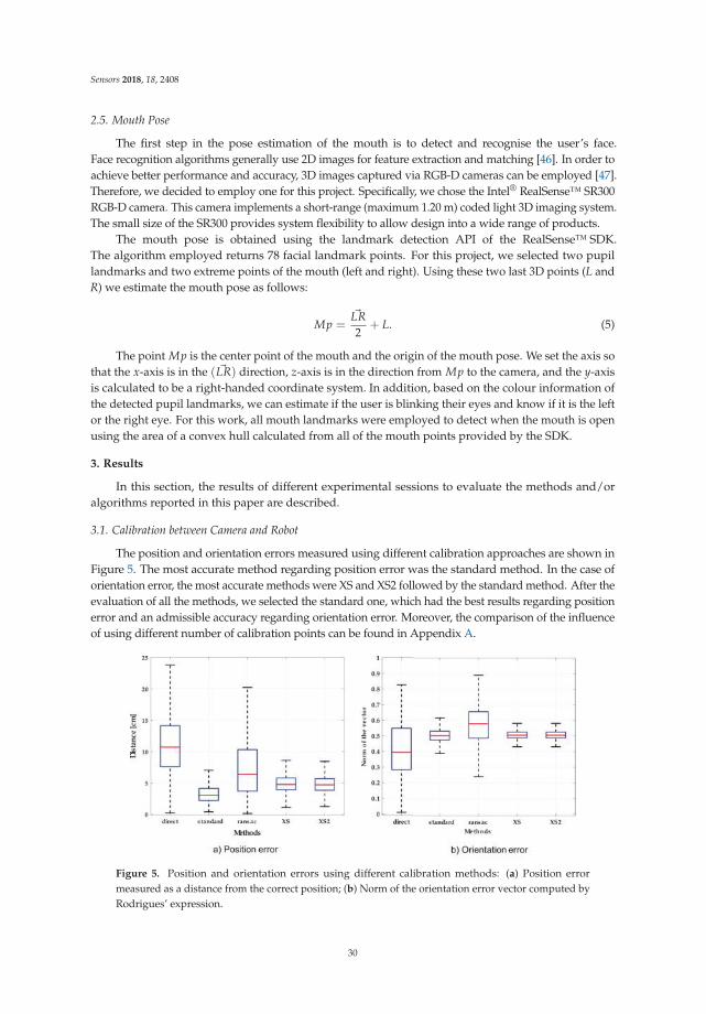
Sensors 2018, 18, 2408

2.5. Mouth Pose

The first step in the pose estimation of the mouth is to detect and recognise the user’s face.Face recognition algorithms generally use 2D images for feature extraction and matching [46]. In order toachieve better performance and accuracy, 3D images captured via RGB-D cameras can be employed [47].Therefore, we decided to employ one for this project. Specifically, we chose the Intel® RealSense™ SR300RGB-D camera. This camera implements a short-range (maximum 1.20 m) coded light 3D imaging system.The small size of the SR300 provides system flexibility to allow design into a wide range of products.

The mouth pose is obtained using the landmark detection API of the RealSense™ SDK.The algorithm employed returns 78 facial landmark points. For this project, we selected two pupillandmarks and two extreme points of the mouth (left and right). Using these two last 3D points (L andR) we estimate the mouth pose as follows:

Mp =�LR

2+ L. (5)

The point Mp is the center point of the mouth and the origin of the mouth pose. We set the axis sothat the x-axis is in the ( �LR) direction, z-axis is in the direction from Mp to the camera, and the y-axisis calculated to be a right-handed coordinate system. In addition, based on the colour information ofthe detected pupil landmarks, we can estimate if the user is blinking their eyes and know if it is the leftor the right eye. For this work, all mouth landmarks were employed to detect when the mouth is openusing the area of a convex hull calculated from all of the mouth points provided by the SDK.

3. Results

In this section, the results of different experimental sessions to evaluate the methods and/oralgorithms reported in this paper are described.

3.1. Calibration between Camera and Robot

The position and orientation errors measured using different calibration approaches are shown inFigure 5. The most accurate method regarding position error was the standard method. In the case oforientation error, the most accurate methods were XS and XS2 followed by the standard method. After theevaluation of all the methods, we selected the standard one, which had the best results regarding positionerror and an admissible accuracy regarding orientation error. Moreover, the comparison of the influenceof using different number of calibration points can be found in Appendix A.

Figure 5. Position and orientation errors using different calibration methods: (a) Position errormeasured as a distance from the correct position; (b) Norm of the orientation error vector computed byRodrigues’ expression.

30

Sensors 2018, 18, 2408

3.2. Detection and Pose Estimation

In this section, the quantitative results of the detection and pose estimation method are described.These results are compared with the works of other authors. Finally, a detailed analysis of thecomputational performance of the algorithm was carried out, and as in the quantitative analysis, it iscompared with the work of other authors.

3.2.1. Quantitative Validation of the Detection and Pose Estimation of 3D Objects

To quantitatively evaluate the developed method, the LINEMOD dataset [24] was used. Althoughthere are other datasets (e.g., T-LESS [48], Tejani [37], among others), the LINEMOD dataset isundoubtedly the most used by the scientific community to quantitatively evaluate detection andpose estimation methods. The LINEMOD dataset is formed by 15 3D non-textured objects, of which13 colour 3D models are available (see Figure 6). Each model has a sequence of RGB-D images (around1200 images in each), in which multiple objects appear from different points of view and distances(in a cluttered environment). Each image has the associated real pose (“ground truth”) of the objectand the intrinsic parameters of the RGB-D camera employed for acquiring the image.

Figure 6. Some 3D models of the LINEMOD dataset.

The most common metrics employed for comparing the different methods are:

• Average distance (AD): This metric was introduced by Hinterstoisser et al. [24] and is the mostemployed to quantitatively evaluate the accuracy of pose estimation [19,26–29,49]. Given a set ofvertices of a 3D model, M, the actual rotation and translation [R, t] (“ground truth ”) and theirestimations [R, t]:

mAD =1

|M| ∑x∈M

||(Rx + T)− (Rx − T)||2. (6)

when the 3D object is symmetrical, like some of the LINEMOD models (“cup”, “bowl”, “box”,and “glue”):

mAD =1

|M| ∑x1∈M

minx2∈M

||(Rx1 + T)− (Rx2 − T)||2. (7)

Traditionally, it is considered that the pose is correct if mAD ≤ kmd, d being the diameter ofthe object, and km a coefficient ≥ 0. Generally a km = 0.1 is used (i.e., 10% of the diameter ofthe object).

• Shotton criteria (5 cm 5◦): Using this criteria [24] a pose is considered correct if the rotational erroris less than five degrees and the translational error is less than 5 cm. Please note that this metricdoes not take the size of the object into account.

• 2D Bounding Box: This metric calculates the intersection over union (IoU) [50] between the 2Dbounding box obtained by projecting all the vertices of the 3D object with the real pose “groundtruth ” in the image and the 2D bounding obtained by projecting all the vertices of the object withthe estimated pose. A pose is correct if IoU > 0.5.

31

Sensors 2018, 18, 2408

• 2D Projections: This metric [36] sets a pose as valid if:

mProj =1

|M| ∑x∈M

||K(Rx + T)− K(Rx − T)||2 (8)

is less than 5 pixels. M is the set of vertices of the 3D model, K is the matrix of intrinsic parameters,[R, t] is the estimated pose and [R, t] is the true pose. It should be noted that this metric is themost appropriate when you want to estimate the pose of 3D objects in an Augmented Realitysystem, and so was not used in this work.

• F1-Score. Given PR as true positive, TPR the recall ratio (true positive rate), and PPV theprecision ratio (positive predictive value), F1 = 2 PR

PPV+TPR is defined. This metric has been usedin References [28,37].

3.2.2. Comparison of the Results with State-Of-The-Art Methods

Firstly, it is worth noting that unlike other authors, quantitative evaluation using the mainmetrics was carried out in this work. This is of vital importance, since the results obtained often varysubstantially depending on the metric employed.

When comparing the results of our method with some of the most popular methods (Table 1) on theLINEMOD dataset and with the AD metric, the results obtained are similar to those of the LINEMOD++method proposed by Hinterstoisser et al. [24] (95.7% versus 96.6%). This is reasonable since the methoddeveloped in this work is based mainly on the LINEMOD++ algorithm. Specifically, the proposed methodpresents a series of modifications of LINEMOD++ in order to optimise the performance in real scenarios.

Looking in detail at the obtained results (see Tables 1 and 2) and comparing with the resultsobtained from other similar works, our method improved upon the results of [17,26,27,35]. It alsoexceeded by a wide margin the method SSD-6D [28], since it got 76.3% using the RGB informationand 90.9% with the RGB-D information compared to the 95.7% obtained in our method. Note alsothat it improved the accuracy of the method of Brachmann et al. [36] when it only used the colourinformation (50.2%). In addition, the described method improved the BB8 [29] method with or withoutrefinement of the pose (62.7%).

On the other hand, it matched the results obtained by the method of Zhang et al. [51]. In contrast,the method of Brachmann et al. [36] was more accurate when the depth information was employedin addition to the colour information; specifically, it achieved 99.0% with the AD metric in theLINEMOD dataset.

When comparing with the work of [19], it is worth remarking that they only show the best resultsof 8 of the 13 3D objects available in the LINEMOD database. Consequently, if we calculate the averageobtained using the AD metric of our method for these models, we obtained 96.5% versus 97.8% of themethod of Hinterstoisser [19].

Finally, it can be concluded that although more precise methods have appeared in recent years [28](all of them based on deep learning techniques), especially when the objects are partially visible, ourmethod was not only accurate enough compared to many of the methods in the scientific literature(see Tables 1 and 2), but it was also (as will be seen in the next section) the fastest of all the methodsanalysed in this work, allowing pose estimation in real-time with only the requirement of a 3D model(not necessarily with colour) of the 3D object.

Additionally, Figure 7 shows some qualitative results of the estimated pose using our method inthe LINEMOD++ database. Specifically, a projection was done of a bounding box calculated using theestimated pose (in green) and the ground truth pose (in red).

32

Sensors 2018, 18, 2408

Table 1. Comparison of the results between different detection and pose estimation methods on theLINEMOD dataset [24] using the AD metric and km = 0.1, given as the percentage of objects in whichthe pose was estimated with an error smaller than 10% of the object diameter.

Sequence Our Method LINEMOD++ [24] Drost [17] Hodan et al. [26] Brachmann et al. [35] Hinterstoisser et al. [19]

Ape 97.3% 95.8% 86.5% 93.9% 85.4% 98.5%Benchwise 95.4% 98.7% 70.7% 99.8% 98.9% 99.8%

Driller 93.0% 93.6% 87.3% 94.1% 99.7% 93.4%Cam 95.0% 97.5% 78.6% 95.5% 92.1% 99.3%Can 97.0% 95.9% 80.2% 95.9% 84.4% 98.7%Iron 98.7% 97.5% 84.9% 97.0% 98.8% 98.3%

Lamp 99.2% 97.7% 93.3% 88.8% 97.6% 96.0%Phone 97.1% 93.3% 80.7% 89.4% 86.1% 98.6%

Cat 98.8% 99.3% 85.4% 98.2% 90.6%Hole punch 92.8% 95.9% 77.4% 88.0% 97.9%

Duck 99.1% 95.9% 46.0% 94.3% 92.7%Cup 97.7% 97.1% 68.4% 99.5%Bowl 97.8% 99.9% 95.7% 98.8%Box 99.2% 99.8% 97.0% 100.0% 91.1%Glue 96.9% 91.8% 57.2% 98.0% 87.9%

Mean 95.7% 96.6% 79.3% 95.4% 92.5% 97.8%

Sequence Zhang et al. [27] Kehl et al. [32] Zhang et al. [51] BB8 [29] SSD-6D with RGB-D [28]

Ape 96.3% 96.9% 93.9%Benchwise 90.4% 94.1% 99.8%

Driller 95.2% 96.2% 94.1%Cam 91.3% 97.7% 95.5%Can 98.2% 95.2% 95.9%Iron 98.8% 98.7% 97.0%

Lamp 91.4% 96.2% 88.8%Phone 92.7% 92.8%

Cat 91.8% 97.4% 98.2%Hole punch 97.8% 96.8% 88.0%

Duck 91.8% 97.3% 94.3%Cup 99.6% 99.6%Bowl 99.9% 99.9%Box 99.8% 99.9% 100.0%Glue 94.6% 78.6% 98.0%

Mean 94.7% 95.8% 95.7% 62.7% 90.9%

Table 2. Results of our detection and pose estimation system on the LINEMOD dataset [24] usingdifferent metrics. The percentage is calculated as the number of times that the pose was estimatedcorrectly with respect to the total number of images for each of the sequences. AD: average distance;IoU: intersection over union.

Model 6D Pose (5 cm 5◦) 6D Pose (AD) 2D Bounding Box (IoU) F1-Score (AD)

Ape (1235) 98.94% 97.33% 98.86% 0.9864Bench Vise (1214) 95.46% 95.46% 95.46% 0.9768

Driller (1187) 93.09% 91.24% 93.85% 0.9542Cam (1200) 95.08% 94.50% 95.17% 0.9717Can (1195) 97.07% 91.88% 97.07% 0.9577Iron (1151) 98.70% 98.00% 98.87% 0.9899

Lamp (1226) 99.26% 98.04% 99.26% 0.9901Phone (1224) 97.11% 97.11% 97.11% 0.9853

Cat (1178) 98.89% 98.89% 98.89% 0.9944Hole punch (1236) 92.80% 91.35% 92.72% 0.9547

Duck (1253) 99.12% 96.96% 99.12% 0.9846Cup (1239) 97.74% 97.74% 97.66% 0.9881Bowl (1232) 97.81% 97.81% 97.81% 0.9889Box (1252) 99.28% 99.28% 99.28% 0.9963Glue (1219) 96.97% 90.26% 96.97% 0.9495

Mean 97.15% 95.72% 97.20% 0.9779

33

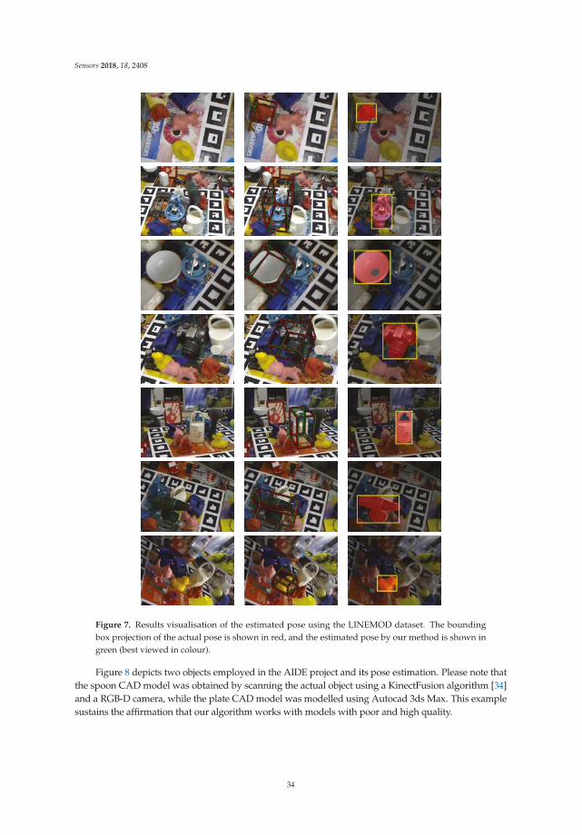
Sensors 2018, 18, 2408

Figure 7. Results visualisation of the estimated pose using the LINEMOD dataset. The boundingbox projection of the actual pose is shown in red, and the estimated pose by our method is shown ingreen (best viewed in colour).

Figure 8 depicts two objects employed in the AIDE project and its pose estimation. Please note thatthe spoon CAD model was obtained by scanning the actual object using a KinectFusion algorithm [34]and a RGB-D camera, while the plate CAD model was modelled using Autocad 3ds Max. This examplesustains the affirmation that our algorithm works with models with poor and high quality.

34

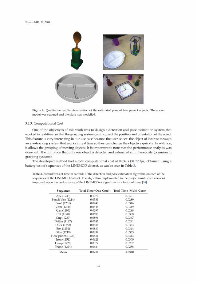
Sensors 2018, 18, 2408

Figure 8. Qualitative results visualisation of the estimated pose of two project objects. The spoonmodel was scanned and the plate was modelled.

3.2.3. Computational Cost

One of the objectives of this work was to design a detection and pose estimation system thatworked in real-time so that the grasping system could correct the position and orientation of the object.This feature is very interesting in our use case because the user selects the object of interest throughan eye-tracking system that works in real time so they can change the objective quickly. In addition,it allows the grasping of moving objects. It is important to note that the performance analysis wasdone with the limitation that only one object is detected and estimated simultaneously (common ingrasping systems).

The developed method had a total computational cost of 0.032 s (31.72 fps) obtained using abattery test of sequences of the LINEMOD dataset, as can be seen in Table 3.

Table 3. Breakdowns of time in seconds of the detection and pose estimation algorithm on each of thesequences of the LINEMOD dataset. The algorithm implemented in the project (multi-core version)improved upon the performance of the LINEMOD++ algorithm by a factor of three [24].

Sequence Total Time (One-Core) Total Time (Multi-Core)

Ape (1235) 0.1070 0.0401Bench Vise (1214) 0.0581 0.0289

Bowl (1231) 0.0748 0.0316Cam (1200) 0.0646 0.0319Can (1195) 0.0597 0.0288Cat (1178) 0.0698 0.0308Cup (1239) 0.0896 0.0367

Driller (1187) 0.0582 0.0291Duck (1253) 0.0836 0.0333Box (1252) 0.0830 0.0344Glue (1219) 0.0837 0.0335

Hole punch (1236) 0.0831 0.0343Iron (1151) 0.0621 0.0300

Lamp (1226) 0.0577 0.0287Phone (1224) 0.0624 0.0288

Mean 0.0731 0.0320

35

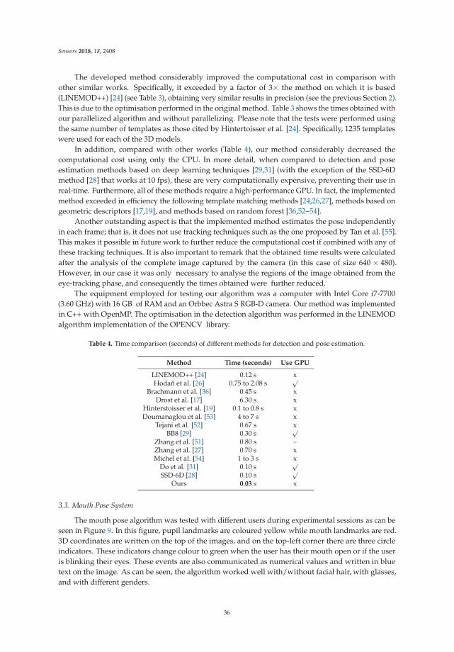
Sensors 2018, 18, 2408

The developed method considerably improved the computational cost in comparison withother similar works. Specifically, it exceeded by a factor of 3× the method on which it is based(LINEMOD++) [24] (see Table 3), obtaining very similar results in precision (see the previous Section 2).This is due to the optimisation performed in the original method. Table 3 shows the times obtained withour parallelized algorithm and without parallelizing. Please note that the tests were performed usingthe same number of templates as those cited by Hintertoisser et al. [24]. Specifically, 1235 templateswere used for each of the 3D models.

In addition, compared with other works (Table 4), our method considerably decreased thecomputational cost using only the CPU. In more detail, when compared to detection and poseestimation methods based on deep learning techniques [29,31] (with the exception of the SSD-6Dmethod [28] that works at 10 fps), these are very computationally expensive, preventing their use inreal-time. Furthermore, all of these methods require a high-performance GPU. In fact, the implementedmethod exceeded in efficiency the following template matching methods [24,26,27], methods based ongeometric descriptors [17,19], and methods based on random forest [36,52–54].

Another outstanding aspect is that the implemented method estimates the pose independentlyin each frame; that is, it does not use tracking techniques such as the one proposed by Tan et al. [55].This makes it possible in future work to further reduce the computational cost if combined with any ofthese tracking techniques. It is also important to remark that the obtained time results were calculatedafter the analysis of the complete image captured by the camera (in this case of size 640 × 480).However, in our case it was only necessary to analyse the regions of the image obtained from theeye-tracking phase, and consequently the times obtained were further reduced.

The equipment employed for testing our algorithm was a computer with Intel Core i7-7700(3.60 GHz) with 16 GB of RAM and an Orbbec Astra S RGB-D camera. Our method was implementedin C++ with OpenMP. The optimisation in the detection algorithm was performed in the LINEMODalgorithm implementation of the OPENCV library.

Table 4. Time comparison (seconds) of different methods for detection and pose estimation.

Method Time (seconds) Use GPU

LINEMOD++ [24] 0.12 s xHodan et al. [26] 0.75 to 2.08 s

√Brachmann et al. [36] 0.45 s x

Drost et al. [17] 6.30 s xHinterstoisser et al. [19] 0.1 to 0.8 s xDoumanaglou et al. [53] 4 to 7 s x

Tejani et al. [52] 0.67 s xBB8 [29] 0.30 s

√Zhang et al. [51] 0.80 s –Zhang et al. [27] 0.70 s xMichel et al. [54] 1 to 3 s x

Do et al. [31] 0.10 s√

SSD-6D [28] 0.10 s√

Ours 0.03 s x

3.3. Mouth Pose System

The mouth pose algorithm was tested with different users during experimental sessions as can beseen in Figure 9. In this figure, pupil landmarks are coloured yellow while mouth landmarks are red.3D coordinates are written on the top of the images, and on the top-left corner there are three circleindicators. These indicators change colour to green when the user has their mouth open or if the useris blinking their eyes. These events are also communicated as numerical values and written in bluetext on the image. As can be seen, the algorithm worked well with/without facial hair, with glasses,and with different genders.

36

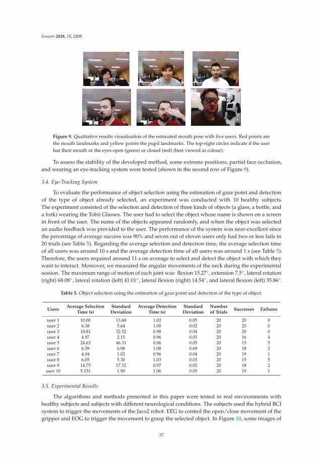
Sensors 2018, 18, 2408

Figure 9. Qualitative results visualisation of the estimated mouth pose with five users. Red points arethe mouth landmarks and yellow points the pupil landmarks. The top-right circles indicate if the userhas their mouth or the eyes open (green) or closed (red) (best viewed in colour).

To assess the stability of the developed method, some extreme positions, partial face occlusion,and wearing an eye-tracking system were tested (shown in the second row of Figure 9).

3.4. Eye-Tracking System

To evaluate the performance of object selection using the estimation of gaze point and detectionof the type of object already selected, an experiment was conducted with 10 healthy subjects.The experiment consisted of the selection and detection of three kinds of objects (a glass, a bottle, anda fork) wearing the Tobii Glasses. The user had to select the object whose name is shown on a screenin front of the user. The name of the objects appeared randomly, and when the object was selectedan audio feedback was provided to the user. The performance of the system was near-excellent sincethe percentage of average success was 90% and seven out of eleven users only had two or less fails in20 trials (see Table 5). Regarding the average selection and detection time, the average selection timeof all users was around 10 s and the average detection time of all users was around 1 s (see Table 5).Therefore, the users required around 11 s on average to select and detect the object with which theywant to interact. Moreover, we measured the angular movements of the neck during the experimentalsession. The maximum range of motion of each joint was: flexion 15.27◦, extension 7.5◦, lateral rotation(right) 68.08◦, lateral rotation (left) 41.01◦, lateral flexion (right) 14.54◦, and lateral flexion (left) 35.86◦.

Table 5. Object selection using the estimation of gaze point and detection of the type of object.

UsersAverage Selection Standard Average Detection Standard Number

Successes FailuresTime (s) Deviation Time (s) Deviation of Trials

user 1 10.00 13.68 1.02 0.05 20 20 0user 2 6.38 5.64 1.00 0.02 20 20 0user 3 18.81 32.52 0.98 0.04 20 20 0user 4 4.97 2.15 0.96 0.05 20 16 4user 5 24.63 46.31 0.96 0.05 20 15 5user 6 6.39 6.98 1.08 0.69 20 18 2user 7 4.04 1.02 0.96 0.04 20 19 1user 8 6.05 5.30 1.03 0.03 20 15 5user 9 14.75 17.32 0.97 0.02 20 18 2user 10 5.151 1.90 1.06 0.05 20 19 1

3.5. Experimental Results

The algorithms and methods presented in this paper were tested in real environments withhealthy subjects and subjects with different neurological conditions. The subjects used the hybrid BCIsystem to trigger the movements of the Jaco2 robot: EEG to control the open/close movement of thegripper and EOG to trigger the movement to grasp the selected object. In Figure 10, some images of

37

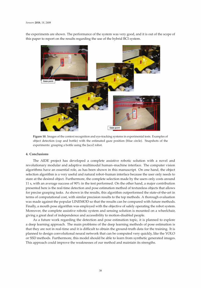
Sensors 2018, 18, 2408

the experiments are shown. The performance of the system was very good, and it is out of the scope ofthis paper to report on the results regarding the use of the hybrid BCI system.

Figure 10. Images of the context recognition and eye-tracking systems in experimental tests. Examples ofobject detection (cup and bottle) with the estimated gaze position (blue circle). Snapshots of theexperiments: grasping a bottle using the Jaco2 robot.

4. Conclusions

The AIDE project has developed a complete assistive robotic solution with a novel andrevolutionary modular and adaptive multimodal human–machine interface. The computer visionalgorithms have an essential role, as has been shown in this manuscript. On one hand, the objectselection algorithm is a very useful and natural robot–human interface because the user only needs tostare at the desired object. Furthermore, the complete selection made by the users only costs around11 s, with an average success of 90% in the test performed. On the other hand, a major contributionpresented here is the real-time detection and pose estimation method of textureless objects that allowsfor precise grasping tasks. As shown in the results, this algorithm outperformed the state-of-the-art interms of computational cost, with similar precision results to the top methods. A thorough evaluationwas made against the popular LINEMOD so that the results can be compared with future methods.Finally, a mouth pose algorithm was employed with the objective of safely operating the robot system.Moreover, the complete assistive robotic system and sensing solution is mounted on a wheelchair,giving a great deal of independence and accessibility to motion-disabled people.

As a future work regarding the detection and pose estimation topic, it is planned to explorea deep learning approach. The main problems of the deep learning methods of pose estimation isthat they are not in real-time and it is difficult to obtain the ground-truth data for the training. It isplanned to design convolutional neural network that can be computed very quickly, like the YOLOor SSD methods. Furthermore, this model should be able to learn from synthetic generated images.This approach could improve the weaknesses of our method and maintain its strengths.

38

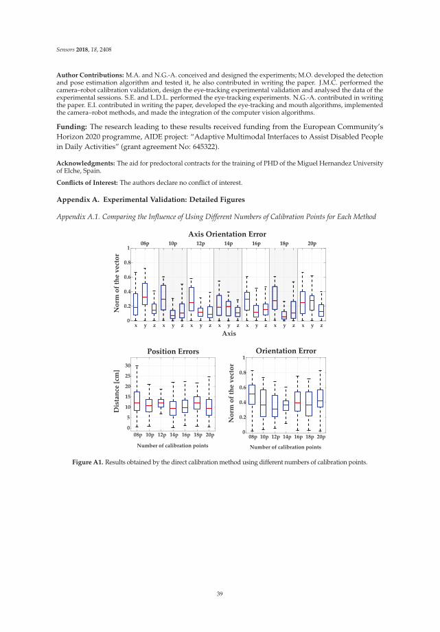
Sensors 2018, 18, 2408

Author Contributions: M.A. and N.G.-A. conceived and designed the experiments; M.O. developed the detectionand pose estimation algorithm and tested it, he also contributed in writing the paper. J.M.C. performed thecamera–robot calibration validation, design the eye-tracking experimental validation and analysed the data of theexperimental sessions. S.E. and L.D.L. performed the eye-tracking experiments. N.G.-A. contributed in writingthe paper. E.I. contributed in writing the paper, developed the eye-tracking and mouth algorithms, implementedthe camera–robot methods, and made the integration of the computer vision algorithms.

Funding: The research leading to these results received funding from the European Community’sHorizon 2020 programme, AIDE project: “Adaptive Multimodal Interfaces to Assist Disabled Peoplein Daily Activities” (grant agreement No: 645322).

Acknowledgments: The aid for predoctoral contracts for the training of PHD of the Miguel Hernandez Universityof Elche, Spain.

Conflicts of Interest: The authors declare no conflict of interest.

Appendix A. Experimental Validation: Detailed Figures

Appendix A.1. Comparing the Influence of Using Different Numbers of Calibration Points for Each Method

08p 10p 12p 14p 16p 18p 20p

0

5

10

15

20

25

30

x y z x y z x y z x y z x y z x y z x y z0

0.2

0.4

0.6

0.8

1

08p 10p 12p 14p 16p 18p 20p0

0.2

0.4

0.6

0.8

1

Number of calibration points

Dis

tan

ce [

cm]

Position Errors

Axis

No

rm o

f th

e v

ect

or

Axis Orientation Error08p 10p 12p 14p 16p 18p 20p

No

rm o

f th

e v

ect

or

Orientation Error

Number of calibration points

Figure A1. Results obtained by the direct calibration method using different numbers of calibration points.

39

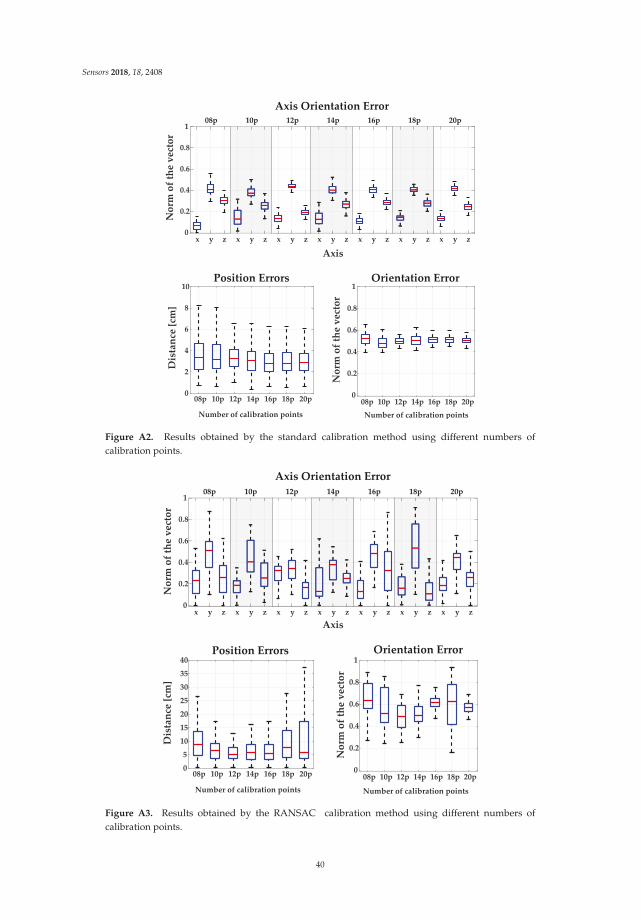
Sensors 2018, 18, 2408

08p 10p 12p 14p 16p 18p 20p0

2

4

6

8

10

x y z x y z x y z x y z x y z x y z x y z0

0.2

0.4

0.6

0.8

1

08p 10p 12p 14p 16p 18p 20p0

0.2

0.4

0.6

0.8

1

Number of calibration points

Dis

tan

ce [

cm]

Position Errors

Axis

No

rm o

f th

e v

ect

or

Axis Orientation Error08p 10p 12p 14p 16p 18p 20p

No

rm o

f th

e v

ect

or

Orientation Error

Number of calibration points

Figure A2. Results obtained by the standard calibration method using different numbers ofcalibration points.

08p 10p 12p 14p 16p 18p 20p0

5

10

15

20

25

30

35

40

x y z x y z x y z x y z x y z x y z x y z0

0.2

0.4

0.6

0.8

1

08p 10p 12p 14p 16p 18p 20p0

0.2

0.4

0.6

0.8

1

Number of calibration points

Dis

tan

ce [

cm]

Position Errors

Axis

No

rm o

f th

e v

ect

or

Axis Orientation Error

08p 10p 12p 14p 16p 18p 20p

No

rm o

f th

e v

ect

or

Orientation Error

Number of calibration points

Figure A3. Results obtained by the RANSAC calibration method using different numbers ofcalibration points.

40

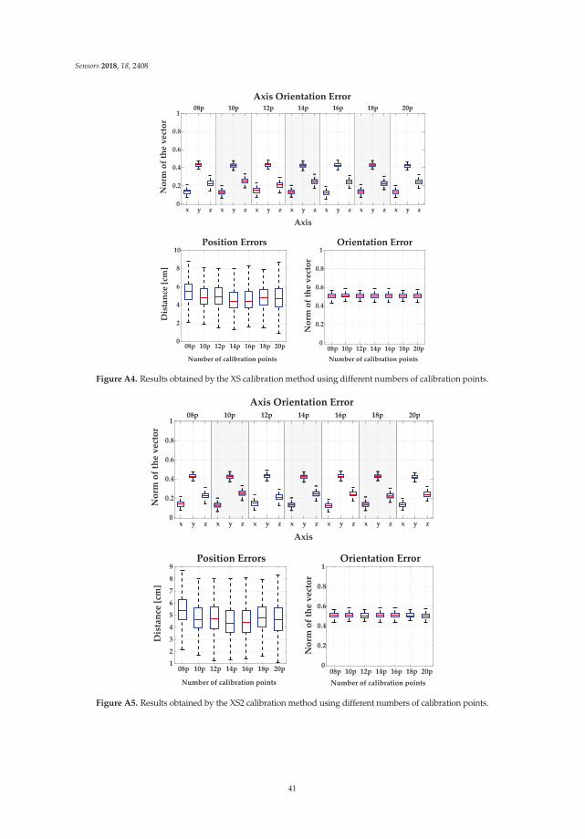
Sensors 2018, 18, 2408

08p 10p 12p 14p 16p 18p 20p0

2

4

6

8

10

x y z x y z x y z x y z x y z x y z x y z0

0.2

0.4

0.6

0.8

1

08p 10p 12p 14p 16p 18p 20p0

0.2

0.4

0.6

0.8

1

Number of calibration points

Dis

tan

ce [

cm]

Position Errors

Axis

No

rm o

f th

e v

ect

or

Axis Orientation Error08p 10p 12p 14p 16p 18p 20p

No

rm o

f th

e v

ect

or

Orientation Error

Number of calibration points

Figure A4. Results obtained by the XS calibration method using different numbers of calibration points.

08p 10p 12p 14p 16p 18p 20p1

2

3

4

5

6

7

8

9

x y z x y z x y z x y z x y z x y z x y z0

0.2

0.4

0.6

0.8

1

08p 10p 12p 14p 16p 18p 20p0

0.2

0.4

0.6

0.8

1

Number of calibration points

Dis

tan

ce [

cm]

Position Errors

Axis

No

rm o

f th

e v

ect

or

Axis Orientation Error08p 10p 12p 14p 16p 18p 20p

No

rm o

f th

e v

ect

or

Orientation Error

Number of calibration points

Figure A5. Results obtained by the XS2 calibration method using different numbers of calibration points.

41

Sensors 2018, 18, 2408

References

1. European Commision. People with disabilities have equal rights. In The European Disability Strategy 2010–2020;Technical Report; European Commision: Washington, DC, USA, 2010.

2. Meng, J.; Zhang, S.; Bekyo, A.; Olsoe, J.; Baxter, B.; He, B. Noninvasive Electroencephalogram Based Controlof a Robotic Arm for Reach and Grasp Tasks. Sci. Rep. 2016, 6, 38565. [CrossRef] [PubMed]

3. Silva, C.; Vongkulbhisal, J.; Marques, M.; Costeira, J.P.; Veloso, M. Feedbot—A Robotic Arm for AutonomousAssisted Feeding. In Proceedings of the Portuguese Conference on Artificial Intelligence, Porto, Portugal,5–8 September 2017; Oliveira, E., Gama, J., Vale, Z., Lopes Cardoso, H., Eds.; Springer InternationalPublishing: Cham, Switzerland, 2017; pp. 486–497.

4. Hochberg, L.R.; Bacher, D.; Jarosiewicz, B.; Masse, N.Y.; Simeral, J.D.; Vogel, J.; Haddadin, S.; Liu, J.;Cash, S.S.; van der Smagt, P.; et al. Reach and grasp by people with tetraplegia using a neurally controlledrobotic arm. Nature 2012, 485, 372. [CrossRef] [PubMed]

5. Collinger, J.L.; Wodlinger, B.; Downey, J.E.; Wang, W.; Tyler-Kabara, E.C.; Weber, D.J.; McMorland, A.J.;Velliste, M.; Boninger, M.L.; Schwartz, A.B. High-performance neuroprosthetic control by an individualwith tetraplegia. Lancet 2013, 381, 557–564. [CrossRef]

6. Pedrocchi, A.; Ferrante, S.; Ambrosini, E.; Gandolla, M.; Casellato, C.; Schauer, T.; Klauer, C.; Pascual, J.;Vidaurre, C.; Gföhler, M.; et al. MUNDUS project: MUltimodal Neuroprosthesis for daily Upper limb Support.J. Neuroeng. Rehabil. 2013, 10, 66. [CrossRef] [PubMed]

7. Frisoli, A.; Sotgiu, E.; Procopio, C.; Chisari, C.; Rossi, B.; Bergamasco, M. Positive effects of rehabilitationtraining with the L-EXOS in chronic stroke. In Proceedings of the SKILLS 2011, Montpellier, France,15–16 December 2011; Volume 1, p. 27.

8. Barsotti, M.; Leonardis, D.; Loconsole, C.; Solazzi, M.; Sotgiu, E.; Procopio, C.; Chisari, C.; Bergamasco, M.;Frisoli, A. A full upper limb robotic exoskeleton for reaching and grasping rehabilitation triggered by MI-BCI.In Proceedings of the 2015 IEEE International Conference on Rehabilitation Robotics (ICORR), Singapore,11–14 August 2015; pp. 49–54.

9. Lauretti, C.; Cordella, F.; Ciancio, A.L.; Trigili, E.; Catalan, J.M.; Badesa, F.J.; Crea, S.; Pagliara, S.M.; Sterzi, S.;Vitiello, N.; et al. Learning by Demonstration for Motion Planning of Upper-Limb Exoskeletons. Front. Neurorobot.

2018, 12. [CrossRef] [PubMed]10. Onose, G.; Grozea, C.; Anghelescu, A.; Daia, C.; Sinescu, C.; Ciurea, A.; Spircu, T.; Mirea, A.; Andone, I.;

Spânu, A. On the Feasibility of Using Motor Imagery EEG-Based Brain–Computer Interface in ChronicTetraplegics for Assistive Robotic Arm Control: A Clinical Test and Long-Term Post-Trial Follow-Up.Spinal Cord 2012, 50, 599. [CrossRef] [PubMed]

11. Li, M.; Yin, H.; Tahara, K.; Billard, A. Learning Object-Level Impedance Control for Robust Grasping andDexterous Manipulation. In Proceedings of the IEEE International Conference on Robotics and Automation,Hong Kong, China, 31 May–7 June 2014; pp. 6784–6791.

12. Ahmadzadeh, S.R.; Kormushev, P.; Caldwell, D.G. Autonomous Robotic Valve Turning: A HierarchicalLearning Approach. In Proceedings of the IEEE International Conference on Robotics and Automation,Karlsruhe, Germany, 6–10 May 2013; pp. 4629–4634.

13. Lowe, D.G. Object recognition from local scale-invariant features. In Proceedings of the 7th IEEE InternationalConference on Computer Vision, Kerkyra, Greece, 20–27 September 1999; Volume 2, pp. 1150–1157.

14. Besl, P.J.; McKay, N.D. A Method for Registration of 3-D Shapes. IEEE Trans. Pattern Anal. Mach. Intell. 1992,14, 239–256, doi:10.1109/34.121791. [CrossRef]

15. Hana, X.F.; Jin, J.S.; Xie, J.; Wang, M.J.; Jiang, W. A comprehensive review of 3D point cloud descriptors.arXiv 2018, arXiv:1802.02297.

16. Rusu, R.B.; Blodow, N.; Beetz, M. Fast point feature histograms (FPFH) for 3D registration. In Proceedingsof the IEEE International Conference on Robotics and Automation (ICRA’09), Kobe, Japan, 12–17 May 2009;pp. 3212–3217.

17. Drost, B.; Ulrich, M.; Navab, N.; Ilic, S. Model globally, match locally: Efficient and robust 3D object recognition.In Proceedings of the 2010 IEEE Conference on Computer Vision and Pattern Recognition (CVPR), San Francisco,CA, USA, 13–18 June 2010; pp. 998–1005.

42

Sensors 2018, 18, 2408

18. Salti, S.; Tombari, F.; Di Stefano, L. SHOT: Unique signatures of histograms for surface and texture description.Comput. Vis. Image Underst. 2014, 125, 251–264. [CrossRef]

19. Hinterstoisser, S.; Lepetit, V.; Rajkumar, N.; Konolige, K. Going further with point pair features. In Proceedingsof the European Conference on Computer Vision, Amsterdam, The Netherlands, 8–16 October 2016; Springer:Cham, Switzerland, 2016; pp. 834–848.

20. Rusu, R.B.; Bradski, G.; Thibaux, R.; Hsu, J. Fast 3d recognition and pose using the viewpoint feature histogram.In Proceedings of the 2010 IEEE/RSJ International Conference on Intelligent Robots and Systems (IROS),Taipei, Taiwan, 18–22 October 2010; pp. 2155–2162.

21. Aldoma, A.; Tombari, F.; Rusu, R.B.; Vincze, M. OUR-CVFH–oriented, unique and repeatable clustered viewpointfeature histogram for object recognition and 6DOF pose estimation. In Proceedings of the Joint DAGM (GermanAssociation for Pattern Recognition) and OAGM Symposium, Graz, Austria, 28–31 August 2012; Springer: Cham,Switzerland, 2012; pp. 113–122.

22. Wohlkinger, W.; Vincze, M. Ensemble of shape functions for 3d object classification. In Proceedings of the 2011IEEE International Conference on Robotics and Biomimetics (ROBIO), Phuket, Thailand, 7–11 December 2011;pp. 2987–2992.

23. Tombari, F.; Salti, S.; Di Stefano, L. A combined texture-shape descriptor for enhanced 3D feature matching.In Proceedings of the 2011 18th IEEE International Conference on Image Processing (ICIP), Brussels, Belgium,11–14 September 2011; pp. 809–812.

24. Hinterstoisser, S.; Lepetit, V.; Ilic, S.; Holzer, S.; Bradski, G.; Konolige, K.; Navab, N. Model Based Training,Detection and Pose Estimation of Texture-Less 3D Objects in Heavily Cluttered Scenes. In Proceedings ofthe Asian Conference on Computer Vision, Daejeon, Korea, 5–9 November 2012; Lee, K.M., Matsushita, Y.,Rehg, J.M., Hu, Z., Eds.; Springer: Berlin/Heidelberg, Germany, 2013; pp. 548–562.

25. Kehl, W.; Tombari, F.; Navab, N.; Ilic, S.; Lepetit, V. Hashmod: A hashing method for scalable 3D objectdetection. arXiv 2016, arXiv:1607.06062.

26. Hodan, T.; Zabulis, X.; Lourakis, M.; Obdržálek, Š.; Matas, J. Detection and fine 3D pose estimation oftexture-less objects in RGB-D images. In Proceedings of the 2015 IEEE/RSJ International Conference onIntelligent Robots and Systems (IROS), Hamburg, Germany, 28 September–3 October 2015; pp. 4421–4428.

27. Zhang, H.; Cao, Q. Texture-less object detection and 6D pose estimation in RGB-D images. Robot. Auton. Syst.

2017, 95, 64–79. [CrossRef]28. Kehl, W.; Manhardt, F.; Tombari, F.; Ilic, S.; Navab, N. SSD-6D: Making RGB-based 3D detection and 6D pose

estimation great again. In Proceedings of the IEEE Conference on Computer Vision and Pattern Recognition(CVPR), Honolulu, HI, USA, 21–26 July 2017; pp. 1521–1529.

29. Rad, M.; Lepetit, V. BB8: A Scalable, Accurate, Robust to Partial Occlusion Method for Predicting the 3DPoses of Challenging Objects without Using Depth. In Proceedings of the International Conference onComputer Vision, Venice, Italy, 22–29 October 2017.

30. Xiang, Y.; Schmidt, T.; Narayanan, V.; Fox, D. PoseCNN: A Convolutional Neural Network for 6D ObjectPose Estimation in Cluttered Scenes. arXiv 2017, arXiv:1711.00199.

31. Do, T.T.; Cai, M.; Pham, T.; Reid, I. Deep-6DPose: Recovering 6D Object Pose from a Single RGB Image.arXiv 2018, arXiv:1802.10367.

32. Kehl, W.; Milletari, F.; Tombari, F.; Ilic, S.; Navab, N. Deep learning of local RGB-D patches for 3D objectdetection and 6D pose estimation. In Proceedings of the European Conference on Computer Vision, Amsterdam,The Netherlands, 8–16 October 2016; Springer: Cham, Switzerland, 2016; pp. 205–220.

33. Hinterstoisser, S.; Lepetit, V.; Wohlhart, P.; Konolige, K. On Pre-Trained Image Features and Synthetic Imagesfor Deep Learning. arXiv 2017, arXiv:1710.10710.

34. Newcombe, R.A.; Izadi, S.; Hilliges, O.; Molyneaux, D.; Kim, D.; Davison, A.J.; Kohi, P.; Shotton, J.;Hodges, S.; Fitzgibbon, A. KinectFusion: Real-Time Dense Surface Mapping and Tracking. In Proceedingsof the 2011 10th IEEE International Symposium on Mixed and Augmented Reality, Basel, Switzerland,26–29 October 2011; pp. 127–136.

43

Sensors 2018, 18, 2408

35. Brachmann, E.; Krull, A.; Michel, F.; Gumhold, S.; Shotton, J.; Rother, C. Learning 6d object pose estimationusing 3d object coordinates. In Proceedings of the European Conference on Computer Vision, Zurich,Switzerland, 6–12 September 2014; Springer: Cham, Switzerland, 2014; pp. 536–551.

36. Brachmann, E.; Michel, F.; Krull, A.; Ying Yang, M.; Gumhold, S. Uncertainty-driven 6d pose estimation ofobjects and scenes from a single rgb image. In Proceedings of the IEEE Conference on Computer Vision andPattern Recognition, Las Vegas, NV, USA, 27–30 June 2016; pp. 3364–3372.

37. Tejani, A.; Tang, D.; Kouskouridas, R.; Kim, T.K. Latent-class hough forests for 3D object detection andpose estimation. In Proceedings of the European Conference on Computer Vision, Zurich, Switzerland,6–12 September 2014; Springer: Cham, Switzerland, 2014; pp. 462–477.

38. Garrido-Jurado, S.; noz Salinas, R.M.; Madrid-Cuevas, F.; Marín-Jiménez, M. Automatic generation anddetection of highly reliable fiducial markers under occlusion. Pattern Recognit. 2014, 47, 2280–2292,doi:10.1016/j.patcog.2014.01.005. [CrossRef]

39. Tabb, A.; Ahmad Yousef, K.M. Solving the Robot-World Hand-Eye(s) Calibration Problem with IterativeMethods. Mach. Vis. Appl. 2017, 28, 569–590. [CrossRef]

40. Cognolato, M.; Graziani, M.; Giordaniello, F.; Saetta, G.; Bassetto, F.; Brugger, P.; Caputo, B.; Müller, H.;Atzori, M. Semi-Automatic Training of an Object Recognition System in Scene Camera Data Using GazeTracking and Accelerometers. In Proceedings of the International Conference on Computer Vision Systems,Copenhagen, Denmark, 6–9 July 2017; Liu, M., Chen, H., Vincze, M., Eds.; Springer International Publishing:Cham, Switzerland, 2017; pp. 175–184.

41. Redmon, J.; Farhadi, A. YOLO9000: Better, Faster, Stronger. In Proceedings of the IEEE Conference ComputerVision and Pattern Recognition (CVPR), Honolulu, HI, USA, 21–26 July 2017; pp. 6517–6525.

42. Ren, S.; He, K.; Girshick, R.; Sun, J. Faster R-CNN: Towards Real-Time Object Detection with Region ProposalNetworks. IEEE Trans. Pattern Anal. Mach. Intell. 2017, 39, 1137–1149, doi:10.1109/TPAMI.2016.2577031.[CrossRef] [PubMed]

43. Liu, W.; Anguelov, D.; Erhan, D.; Szegedy, C.; Reed, S.; Fu, C.Y.; Berg, A.C. SSD: Single Shot MultiBoxDetector. In Proceedings of the European Conference on Computer Vision, Amsterdam, The Netherlands,8–16 October 2016.

44. Lin, T.Y.; Maire, M.; Belongie, S.; Hays, J.; Perona, P.; Ramanan, D.; Dollár, P.; Zitnick, C.L. Microsoft coco:Common objects in context. In Proceedings of the European Conference on Computer Vision, Zurich,Switzerland, 6–12 September 2014; Springer: Cham, Switzerland, 2014; pp. 740–755.

45. Hinterstoisser, S.; Cagniart, C.; Ilic, S.; Sturm, P.; Navab, N.; Fua, P.; Lepetit, V. Gradient response maps forreal-time detection of textureless objects. IEEE Trans. Pattern Anal. Mach. Intell. 2012, 34, 876–888. [CrossRef][PubMed]

46. Zhao, W.; Chellappa, R.; Phillips, P.J.; Rosenfeld, A. Face Recognition: A Literature Survey. ACM Comput.

Surv. (CSUR) 2003, 35, 399–458. [CrossRef]47. Goswami, G.; Bharadwaj, S.; Vatsa, M.; Singh, R. On RGB-D Face Recognition Using Kinect. In Proceedings

of the IEEE Sixth International Conference on Biometrics: Theory, Applications and Systems, Arlington, VA,USA, 29 September–2 October 2013; pp. 1–6.

48. Hodan, T.; Haluza, P.; Obdržálek, Š.; Matas, J.; Lourakis, M.; Zabulis, X. T-LESS: An RGB-D Dataset for 6DPose Estimation of Texture-less Objects. In Proceedings of the IEEE Winter Conference on Applications ofComputer Vision (WACV), Santa Rosa, CA, USA, 24–31 March 2017.

49. Tekin, B.; Sinha, S.N.; Fua, P. Real-Time Seamless Single Shot 6D Object Pose Prediction. arXiv 2017,arXiv:1711.08848.

50. Everingham, M.; Van Gool, L.; Williams, C.K.; Winn, J.; Zisserman, A. The pascal visual object classes (voc)challenge. Int. J. Comput. Vis. 2010, 88, 303–338. [CrossRef]

51. Zhang, H.; Cao, Q. Combined Holistic and Local Patches for Recovering 6D Object Pose. In Proceedings ofthe IEEE Conference on Computer Vision and Pattern Recognition, Honolulu, HI, USA, 21–26 July 2017;pp. 2219–2227.

52. Tejani, A.; Kouskouridas, R.; Doumanoglou, A.; Tang, D.; Kim, T.K. Latent-Class Hough Forests for 6 DoFObject Pose Estimation. IEEE Trans. Pattern Anal. Mach. Intell. 2018, 40, 119–132. [CrossRef] [PubMed]

44

Sensors 2018, 18, 2408

53. Doumanoglou, A.; Kouskouridas, R.; Malassiotis, S.; Kim, T.K. Recovering 6D object pose and predictingnext-best-view in the crowd. In Proceedings of the IEEE Conference on Computer Vision and PatternRecognition, Las Vegas, NV, USA, 27–30 June 2016; pp. 3583–3592.

54. Michel, F.; Kirillov, A.; Brachmann, E.; Krull, A.; Gumhold, S.; Savchynskyy, B.; Rother, C. Global hypothesisgeneration for 6D object pose estimation. In Proceedings of the IEEE Conference on Computer Vision andPattern Recognition, Honolulu, HI, USA, 21–26 July 2017

55. Tan, D.J.; Navab, N.; Tombari, F. Looking beyond the simple scenarios: Combining learners and optimizersin 3d temporal tracking. IEEE Trans. Vis. Comput. Graph. 2017, 23, 2399–2409. [CrossRef] [PubMed]

© 2018 by the authors. Licensee MDPI, Basel, Switzerland. This article is an open accessarticle distributed under the terms and conditions of the Creative Commons Attribution(CC BY) license (http://creativecommons.org/licenses/by/4.0/).

45

Article

ED-FNN: A New Deep Learning Algorithm to DetectPercentage of the Gait Cycle for Powered Prostheses

Huong Thi Thu Vu *,†, Felipe Gomez †, Pierre Cherelle, Dirk Lefeber and Ann Nowé

and Bram Vanderborght

Robotics & MultiBody Mechanics Research Group (R& MM) and Artificial Intelligence Lab, Vrije UniversiteitBrussel and Flanders Make; Pleinlaan 2, 1050 Brussel, Belgium; felipe.gomez.marulanda@vub.ac.be (F.G.);pierre.cherelle@vub.ac.be (P.C.); dlefeber@vub.ac.be (D.L.); ann.nowe@vub.ac.be (A.N.);Bram.Vanderborght@vub.be (B.V.)* Correspondence: vu.huong@vub.ac.be† These authors contributed equally to this work.

Received: 11 June 2018 ; Accepted: 20 July 2018 ; Published: 23 July 2018

Abstract: Throughout the last decade, a whole new generation of powered transtibial prostheses andexoskeletons has been developed. However, these technologies are limited by a gait phase detectionwhich controls the wearable device as a function of the activities of the wearer. Consequently,gait phase detection is considered to be of great importance, as achieving high detection accuracy willproduce a more precise, stable, and safe rehabilitation device. In this paper, we propose a novel gaitpercent detection algorithm that can predict a full gait cycle discretised within a 1% interval. We calledthis algorithm an exponentially delayed fully connected neural network (ED-FNN). A dataset wasobtained from seven healthy subjects that performed daily walking activities on the flat ground anda 15-degree slope. The signals were taken from only one inertial measurement unit (IMU) attachedto the lower shank. The dataset was divided into training and validation datasets for every subject,and the mean square error (MSE) error between the model prediction and the real percentage ofthe gait was computed. An average MSE of 0.00522 was obtained for every subject in both trainingand validation sets, and an average MSE of 0.006 for the training set and 0.0116 for the validationset was obtained when combining all subjects’ signals together. Although our experiments wereconducted in an offline setting, due to the forecasting capabilities of the ED-FNN, our system providesan opportunity to eliminate detection delays for real-time applications.

Keywords: gait phase prediction; gait event detection; lower limb prosthesis; exoskeleton;gait recognition

1. Introduction

Gait phase detection is a non-trivial problem for the new generation of powered prostheses andexoskeletons that are under development [1]. Gait phase detection algorithms are used to create andimprove control strategies that permit prosthetic devices such as those presented in References [2–5]to work with more precision, safety, and stability. The objective of gait event detection algorithmsis to detect non-delayed events in order to build control strategies for improving gait movement.For example, authors in [2] focused on a treatment to fix the amputee’s foot in the lifted position byan orthosis. The technology known as functional electrical stimulation (FES) facilitates the artificialgeneration of action potentials in subcutaneous efferent nerves during the swing phase of the pareticfoot by applying tiny electrical pulses via skin electrodes or implanted electrodes. By modulatingthe frequency or dimensions of these pulses, one can control the contraction of paretic muscles andinduce movements in the affected limbs based on gait phase transitions. The foot pitch and roll anglesare assessed in real-time by means of an inertial measurement unit (IMU). They detected four phases

Sensors 2018, 18, 2389; doi:10.3390/s18072389 www.mdpi.com/journal/sensors46

Sensors 2018, 18, 2389

based on measuring the angular velocity and accelerometer to control the pitch and roll of the foot.Another example is the Ankle Mimicking Prosthetic Foot (AMP-Foot) [4]. This device greatly relieson the accuracy of a gait event detection algorithm to precisely control the torque of the motor inthe device. This device stores energy in the springs during the first event of gait from initial-contact(IC) to foot-flat (FF), then releases the energy stored in the push-off (PO) spring and transmits it tothe ankle joint by controlling the direct-current (DC) of the motor at the moment of heel-off (HO).This joint effort provides a peak torque and power output to the amputee, producing a toe-off (TO)event. After the TO, the amputee enters a swing phase where the torque of the motor is returned to zeromagnitude, allowing the foot to go back to its initial position, resulting in an IC event. Knowing whenall these events take place allows the device to take action at the right moment. Due to the different gaitterminologies used in different articles, in this paper we follow the wording of Figure 1. In this figure,a gait cycle percent is defined as a sample from the continuous space of the gait cycle, an event is viewedas a discrete representation of the percentage space, often labelled as IC, FF, HO and TO; a gait period isconsidered as an interval between events, and a phase is considered as a union of several periods thatrepresent different stages of the gait cycle. Lastly, a full gait cycle is composed of a stance phase anda swing phase. A more detailed description of different gait events is provided in Section 3. In the gaitpercent detection literature, a large set of techniques for improving the performance of event and phasedetection can be found. These include threshold-based methods [3,6–8], time-frequency analysis [9,10],peak heuristic algorithms [9,11,12], machine learning (ML) models [13–21], and combinations ofthese [22]. ML algorithms are among the most popular techniques to detect phases in off-line data(i.e., stored data) and for real-time data (i.e., data gathered in real time). For instance, authors inReferences [17,19] detected four event-phases using hidden Markov models (HMMs). Evans andArvind [23] increased the number of event-phases to five, and applied a hybrid method that combinedfully connected neural networks (FNNs) and HMMs. The model accuracy of these algorithms isdependent on the type of sensors used to gather the gait event signals. Currently, wearable sensorsare widely used for gait phase recognition systems: wearable sensors such as foot switches [14,24,25],foot pressure insoles [6,16,26,27], electromyography (EMG) [28,29], IMUs [3,8,9,15,30–34], and jointangular sensors [20,21] are used specifically for gait detection. A review in [35] showed that footswitches and foot pressure insoles yield the highest accuracy for gait phase detection algorithms.However, these sensors are very sensitive to the placement of the insole, which can influence theaccuracy and reliability of the model. Additionally, they have a short lifespan, as they are often exposedto shock forces of the gait. Consequently, foot switches and foot pressure sensors are not consideredsuitable for daily activity applications. In contrast, Joshi et al. used EMG sensors to accurately extractup to eight gait phases [29]. EMGs are sensors that measure specific muscle activities occurring duringa task. Regardless of the amount of information that can be extracted from the EMG signals, a heavypre-processing step (e.g., a complex combination of filters) is required before it can be directly used ina learning algorithm. Furthermore, these sensors are susceptible to artifacts generated by moisture thatbuilds between the skin and the sensors, and to the way in which they are placed on the skin of thesubject. Recently, IMUs including gyroscopes, accelerometers, and magnetometers have become morepopular, as they are not affected by most of the limitations of the aforementioned sensors. IMUs arelow-cost, low-energy, durable, and can be easily mounted on different parts of the human body.Moreover, a human walking gait is a periodic cycle where IMUs can measure the angular velocitiesand accelerations of the walking gait. As a result, these signals are composed of rich informationthat can be used to accurately predict the gait events. Similar to EMG signals, IMU signals are verysensitive to movement artifacts. This means that in some cases these signals may require a strongpre-processing step before they can be directly used for learning. We hypothesise that deep learningalgorithms are best suited for gait phase detection using IMU signals, as they perform well on signalsthat have a medium-low signal-to-noise ratio.

47

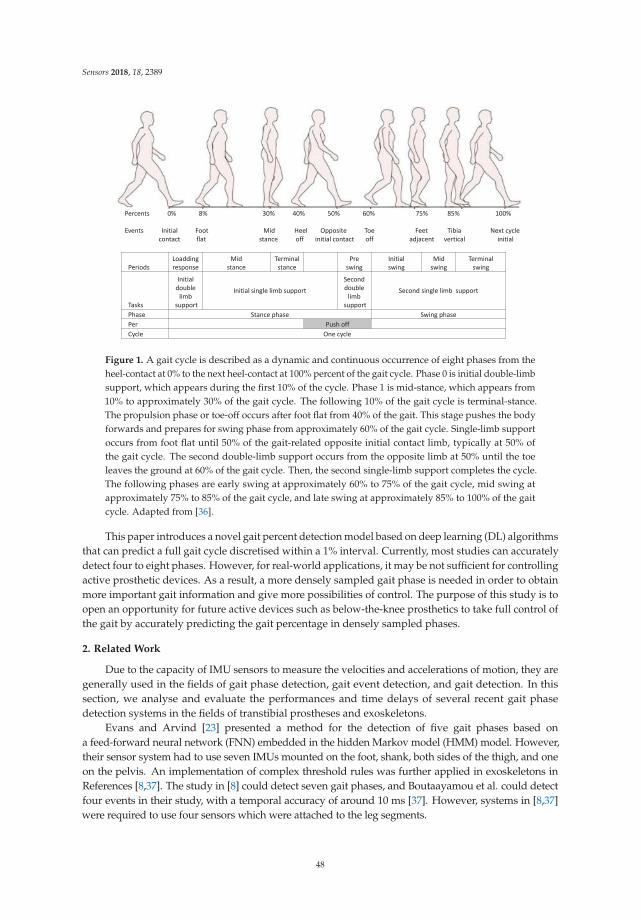
Sensors 2018, 18, 2389

Percents 0% 8% 30% 40% 50% 60% 75% 85% 100%

Events Initial Foot Mid Heel Opposite Toe Feet Tibia Next cyclecontact flat stance off initial contact off adjacent vertical initial

PeriodsLoaddingresponse

Midstance

Terminalstance

Preswing

Initial swing

Midswing

Terminalswing

Tasks

Initial double

limbsupport

Initial single limb supportSeconddouble

limbsupport

Second single limb support

Phase Stance phase Swing phasePer Push offCycle One cycle

Figure 1. A gait cycle is described as a dynamic and continuous occurrence of eight phases from theheel-contact at 0% to the next heel-contact at 100% percent of the gait cycle. Phase 0 is initial double-limbsupport, which appears during the first 10% of the cycle. Phase 1 is mid-stance, which appears from10% to approximately 30% of the gait cycle. The following 10% of the gait cycle is terminal-stance.The propulsion phase or toe-off occurs after foot flat from 40% of the gait. This stage pushes the bodyforwards and prepares for swing phase from approximately 60% of the gait cycle. Single-limb supportoccurs from foot flat until 50% of the gait-related opposite initial contact limb, typically at 50% ofthe gait cycle. The second double-limb support occurs from the opposite limb at 50% until the toeleaves the ground at 60% of the gait cycle. Then, the second single-limb support completes the cycle.The following phases are early swing at approximately 60% to 75% of the gait cycle, mid swing atapproximately 75% to 85% of the gait cycle, and late swing at approximately 85% to 100% of the gaitcycle. Adapted from [36].

This paper introduces a novel gait percent detection model based on deep learning (DL) algorithmsthat can predict a full gait cycle discretised within a 1% interval. Currently, most studies can accuratelydetect four to eight phases. However, for real-world applications, it may be not sufficient for controllingactive prosthetic devices. As a result, a more densely sampled gait phase is needed in order to obtainmore important gait information and give more possibilities of control. The purpose of this study is toopen an opportunity for future active devices such as below-the-knee prosthetics to take full control ofthe gait by accurately predicting the gait percentage in densely sampled phases.

2. Related Work

Due to the capacity of IMU sensors to measure the velocities and accelerations of motion, they aregenerally used in the fields of gait phase detection, gait event detection, and gait detection. In thissection, we analyse and evaluate the performances and time delays of several recent gait phasedetection systems in the fields of transtibial prostheses and exoskeletons.

Evans and Arvind [23] presented a method for the detection of five gait phases based ona feed-forward neural network (FNN) embedded in the hidden Markov model (HMM) model. However,their sensor system had to use seven IMUs mounted on the foot, shank, both sides of the thigh, and oneon the pelvis. An implementation of complex threshold rules was further applied in exoskeletons inReferences [8,37]. The study in [8] could detect seven gait phases, and Boutaayamou et al. could detectfour events in their study, with a temporal accuracy of around 10 ms [37]. However, systems in [8,37]were required to use four sensors which were attached to the leg segments.

48

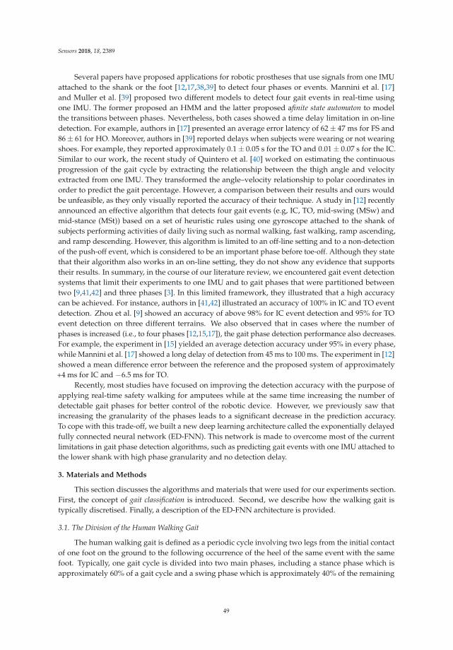
Sensors 2018, 18, 2389

Several papers have proposed applications for robotic prostheses that use signals from one IMUattached to the shank or the foot [12,17,38,39] to detect four phases or events. Mannini et al. [17]and Muller et al. [39] proposed two different models to detect four gait events in real-time usingone IMU. The former proposed an HMM and the latter proposed afinite state automaton to modelthe transitions between phases. Nevertheless, both cases showed a time delay limitation in on-linedetection. For example, authors in [17] presented an average error latency of 62 ± 47 ms for FS and86 ± 61 for HO. Moreover, authors in [39] reported delays when subjects were wearing or not wearingshoes. For example, they reported approximately 0.1 ± 0.05 s for the TO and 0.01 ± 0.07 s for the IC.Similar to our work, the recent study of Quintero et al. [40] worked on estimating the continuousprogression of the gait cycle by extracting the relationship between the thigh angle and velocityextracted from one IMU. They transformed the angle–velocity relationship to polar coordinates inorder to predict the gait percentage. However, a comparison between their results and ours wouldbe unfeasible, as they only visually reported the accuracy of their technique. A study in [12] recentlyannounced an effective algorithm that detects four gait events (e.g, IC, TO, mid-swing (MSw) andmid-stance (MSt)) based on a set of heuristic rules using one gyroscope attached to the shank ofsubjects performing activities of daily living such as normal walking, fast walking, ramp ascending,and ramp descending. However, this algorithm is limited to an off-line setting and to a non-detectionof the push-off event, which is considered to be an important phase before toe-off. Although they statethat their algorithm also works in an on-line setting, they do not show any evidence that supportstheir results. In summary, in the course of our literature review, we encountered gait event detectionsystems that limit their experiments to one IMU and to gait phases that were partitioned betweentwo [9,41,42] and three phases [3]. In this limited framework, they illustrated that a high accuracycan be achieved. For instance, authors in [41,42] illustrated an accuracy of 100% in IC and TO eventdetection. Zhou et al. [9] showed an accuracy of above 98% for IC event detection and 95% for TOevent detection on three different terrains. We also observed that in cases where the number ofphases is increased (i.e., to four phases [12,15,17]), the gait phase detection performance also decreases.For example, the experiment in [15] yielded an average detection accuracy under 95% in every phase,while Mannini et al. [17] showed a long delay of detection from 45 ms to 100 ms. The experiment in [12]showed a mean difference error between the reference and the proposed system of approximately+4 ms for IC and −6.5 ms for TO.

Recently, most studies have focused on improving the detection accuracy with the purpose ofapplying real-time safety walking for amputees while at the same time increasing the number ofdetectable gait phases for better control of the robotic device. However, we previously saw thatincreasing the granularity of the phases leads to a significant decrease in the prediction accuracy.To cope with this trade-off, we built a new deep learning architecture called the exponentially delayedfully connected neural network (ED-FNN). This network is made to overcome most of the currentlimitations in gait phase detection algorithms, such as predicting gait events with one IMU attached tothe lower shank with high phase granularity and no detection delay.

3. Materials and Methods

This section discusses the algorithms and materials that were used for our experiments section.First, the concept of gait classification is introduced. Second, we describe how the walking gait istypically discretised. Finally, a description of the ED-FNN architecture is provided.

3.1. The Division of the Human Walking Gait

The human walking gait is defined as a periodic cycle involving two legs from the initial contactof one foot on the ground to the following occurrence of the heel of the same event with the samefoot. Typically, one gait cycle is divided into two main phases, including a stance phase which isapproximately 60% of a gait cycle and a swing phase which is approximately 40% of the remaining

49

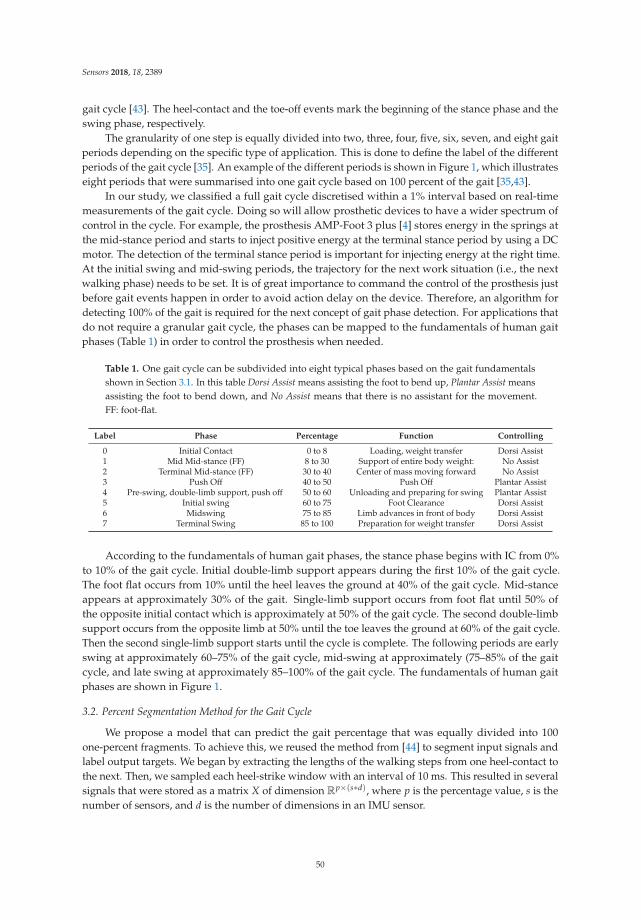
Sensors 2018, 18, 2389

gait cycle [43]. The heel-contact and the toe-off events mark the beginning of the stance phase and theswing phase, respectively.

The granularity of one step is equally divided into two, three, four, five, six, seven, and eight gaitperiods depending on the specific type of application. This is done to define the label of the differentperiods of the gait cycle [35]. An example of the different periods is shown in Figure 1, which illustrateseight periods that were summarised into one gait cycle based on 100 percent of the gait [35,43].

In our study, we classified a full gait cycle discretised within a 1% interval based on real-timemeasurements of the gait cycle. Doing so will allow prosthetic devices to have a wider spectrum ofcontrol in the cycle. For example, the prosthesis AMP-Foot 3 plus [4] stores energy in the springs atthe mid-stance period and starts to inject positive energy at the terminal stance period by using a DCmotor. The detection of the terminal stance period is important for injecting energy at the right time.At the initial swing and mid-swing periods, the trajectory for the next work situation (i.e., the nextwalking phase) needs to be set. It is of great importance to command the control of the prosthesis justbefore gait events happen in order to avoid action delay on the device. Therefore, an algorithm fordetecting 100% of the gait is required for the next concept of gait phase detection. For applications thatdo not require a granular gait cycle, the phases can be mapped to the fundamentals of human gaitphases (Table 1) in order to control the prosthesis when needed.

Table 1. One gait cycle can be subdivided into eight typical phases based on the gait fundamentalsshown in Section 3.1. In this table Dorsi Assist means assisting the foot to bend up, Plantar Assist meansassisting the foot to bend down, and No Assist means that there is no assistant for the movement.FF: foot-flat.

Label Phase Percentage Function Controlling

0 Initial Contact 0 to 8 Loading, weight transfer Dorsi Assist1 Mid Mid-stance (FF) 8 to 30 Support of entire body weight: No Assist2 Terminal Mid-stance (FF) 30 to 40 Center of mass moving forward No Assist3 Push Off 40 to 50 Push Off Plantar Assist4 Pre-swing, double-limb support, push off 50 to 60 Unloading and preparing for swing Plantar Assist5 Initial swing 60 to 75 Foot Clearance Dorsi Assist6 Midswing 75 to 85 Limb advances in front of body Dorsi Assist7 Terminal Swing 85 to 100 Preparation for weight transfer Dorsi Assist

According to the fundamentals of human gait phases, the stance phase begins with IC from 0%to 10% of the gait cycle. Initial double-limb support appears during the first 10% of the gait cycle.The foot flat occurs from 10% until the heel leaves the ground at 40% of the gait cycle. Mid-stanceappears at approximately 30% of the gait. Single-limb support occurs from foot flat until 50% ofthe opposite initial contact which is approximately at 50% of the gait cycle. The second double-limbsupport occurs from the opposite limb at 50% until the toe leaves the ground at 60% of the gait cycle.Then the second single-limb support starts until the cycle is complete. The following periods are earlyswing at approximately 60–75% of the gait cycle, mid-swing at approximately (75–85% of the gaitcycle, and late swing at approximately 85–100% of the gait cycle. The fundamentals of human gaitphases are shown in Figure 1.

3.2. Percent Segmentation Method for the Gait Cycle

We propose a model that can predict the gait percentage that was equally divided into 100one-percent fragments. To achieve this, we reused the method from [44] to segment input signals andlabel output targets. We began by extracting the lengths of the walking steps from one heel-contact tothe next. Then, we sampled each heel-strike window with an interval of 10 ms. This resulted in severalsignals that were stored as a matrix X of dimension R

p×(s∗d), where p is the percentage value, s is thenumber of sensors, and d is the number of dimensions in an IMU sensor.

50

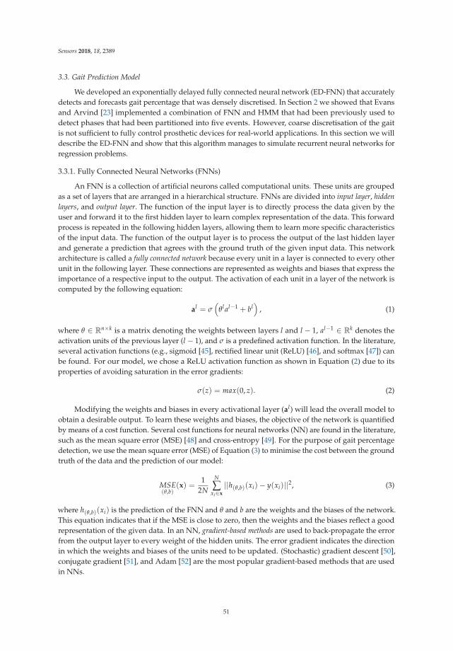
Sensors 2018, 18, 2389

3.3. Gait Prediction Model

We developed an exponentially delayed fully connected neural network (ED-FNN) that accuratelydetects and forecasts gait percentage that was densely discretised. In Section 2 we showed that Evansand Arvind [23] implemented a combination of FNN and HMM that had been previously used todetect phases that had been partitioned into five events. However, coarse discretisation of the gaitis not sufficient to fully control prosthetic devices for real-world applications. In this section we willdescribe the ED-FNN and show that this algorithm manages to simulate recurrent neural networks forregression problems.

3.3.1. Fully Connected Neural Networks (FNNs)

An FNN is a collection of artificial neurons called computational units. These units are groupedas a set of layers that are arranged in a hierarchical structure. FNNs are divided into input layer, hidden

layers, and output layer. The function of the input layer is to directly process the data given by theuser and forward it to the first hidden layer to learn complex representation of the data. This forwardprocess is repeated in the following hidden layers, allowing them to learn more specific characteristicsof the input data. The function of the output layer is to process the output of the last hidden layerand generate a prediction that agrees with the ground truth of the given input data. This networkarchitecture is called a fully connected network because every unit in a layer is connected to every otherunit in the following layer. These connections are represented as weights and biases that express theimportance of a respective input to the output. The activation of each unit in a layer of the network iscomputed by the following equation:

al = σ(

θlal−1 + bl)

, (1)

where θ ∈ Rn×k is a matrix denoting the weights between layers l and l − 1, al−1 ∈ R

k denotes theactivation units of the previous layer (l − 1), and σ is a predefined activation function. In the literature,several activation functions (e.g., sigmoid [45], rectified linear unit (ReLU) [46], and softmax [47]) canbe found. For our model, we chose a ReLU activation function as shown in Equation (2) due to itsproperties of avoiding saturation in the error gradients:

σ(z) = max(0, z). (2)

Modifying the weights and biases in every activational layer (al) will lead the overall model toobtain a desirable output. To learn these weights and biases, the objective of the network is quantifiedby means of a cost function. Several cost functions for neural networks (NN) are found in the literature,such as the mean square error (MSE) [48] and cross-entropy [49]. For the purpose of gait percentagedetection, we use the mean square error (MSE) of Equation (3) to minimise the cost between the groundtruth of the data and the prediction of our model:

MSE(θ,b)

(x) =1

2N

N

∑xi∈x

||h(θ,b)(xi)− y(xi)||2, (3)

where h(θ,b)(xi) is the prediction of the FNN and θ and b are the weights and the biases of the network.This equation indicates that if the MSE is close to zero, then the weights and the biases reflect a goodrepresentation of the given data. In an NN, gradient-based methods are used to back-propagate the errorfrom the output layer to every weight of the hidden units. The error gradient indicates the directionin which the weights and biases of the units need to be updated. (Stochastic) gradient descent [50],conjugate gradient [51], and Adam [52] are the most popular gradient-based methods that are usedin NNs.

51

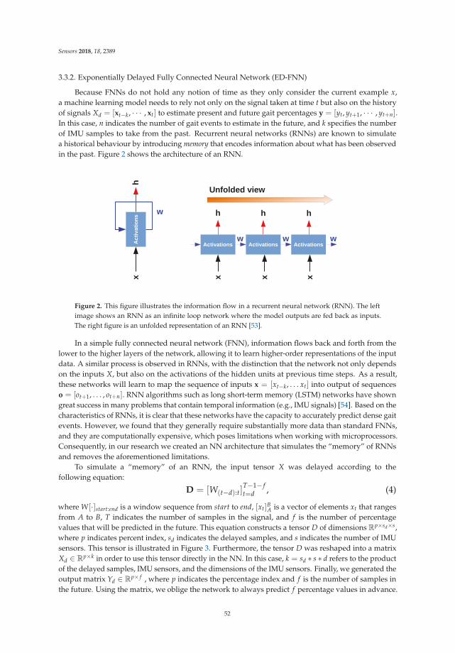
Sensors 2018, 18, 2389

3.3.2. Exponentially Delayed Fully Connected Neural Network (ED-FNN)

Because FNNs do not hold any notion of time as they only consider the current example x,a machine learning model needs to rely not only on the signal taken at time t but also on the historyof signals Xd = [xt−k, · · · , xt] to estimate present and future gait percentages y = [yt, yt+1, · · · , yt+n].In this case, n indicates the number of gait events to estimate in the future, and k specifies the numberof IMU samples to take from the past. Recurrent neural networks (RNNs) are known to simulatea historical behaviour by introducing memory that encodes information about what has been observedin the past. Figure 2 shows the architecture of an RNN.

Figure 2. This figure illustrates the information flow in a recurrent neural network (RNN). The leftimage shows an RNN as an infinite loop network where the model outputs are fed back as inputs.The right figure is an unfolded representation of an RNN [53].

In a simple fully connected neural network (FNN), information flows back and forth from thelower to the higher layers of the network, allowing it to learn higher-order representations of the inputdata. A similar process is observed in RNNs, with the distinction that the network not only dependson the inputs X, but also on the activations of the hidden units at previous time steps. As a result,these networks will learn to map the sequence of inputs x = [xt−k, . . . xt] into output of sequenceso = [ot+1, . . . , ot+n]. RNN algorithms such as long short-term memory (LSTM) networks have showngreat success in many problems that contain temporal information (e.g., IMU signals) [54]. Based on thecharacteristics of RNNs, it is clear that these networks have the capacity to accurately predict dense gaitevents. However, we found that they generally require substantially more data than standard FNNs,and they are computationally expensive, which poses limitations when working with microprocessors.Consequently, in our research we created an NN architecture that simulates the “memory” of RNNsand removes the aforementioned limitations.

To simulate a “memory” of an RNN, the input tensor X was delayed according to thefollowing equation:

D = [W(t−d):t]T−1− ft=d , (4)

where W[·]start:end is a window sequence from start to end, [xt]BA is a vector of elements xt that rangesfrom A to B, T indicates the number of samples in the signal, and f is the number of percentagevalues that will be predicted in the future. This equation constructs a tensor D of dimensions Rp×sd×s,where p indicates percent index, sd indicates the delayed samples, and s indicates the number of IMUsensors. This tensor is illustrated in Figure 3. Furthermore, the tensor D was reshaped into a matrixXd ∈ R

p×k in order to use this tensor directly in the NN. In this case, k = sd ∗ s ∗ d refers to the productof the delayed samples, IMU sensors, and the dimensions of the IMU sensors. Finally, we generated theoutput matrix Yd ∈ R

p× f , where p indicates the percentage index and f is the number of samples inthe future. Using the matrix, we oblige the network to always predict f percentage values in advance.

52

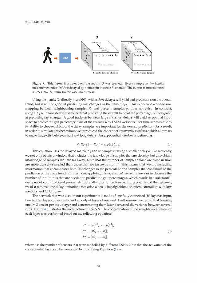
Sensors 2018, 18, 2389

Figure 3. This figure illustrates how the matrix D was created. Every sample in the inertialmeasurement unit (IMU) is delayed by n times (in this case five times). The output matrix is shiftedn times into the future (in this case three times).

Using the matrix Xd directly in an FNN with a short delay d will yield bad predictions on the overalltrend, but it will be good at predicting fast changes in the percentage. This is because a one-to-onemapping between neighbouring samples Xd and percent samples yd does not exist. In contrast,using a Xd with long delays will be better at predicting the overall trend of the percentage, but less goodat predicting fast changes. A good trade-off between large and short delays will yield an optimal inputspace to predict the gait percentage. One of the reasons why LSTM works well for time series is due toits ability to choose which of the delay samples are important for the overall prediction. As a result,in order to simulate this behaviour, we introduced the concept of exponential windows, which allows usto make trade-offs between short and long delays. An exponential window is defined as:

ψ(Xd, δ) = Xd[t − exp(k)]δk=0. (5)

This equation uses the delayed matrix Xd and re-samples it using a smaller delay δ. Consequently,we not only obtain a window that includes the knowledge of samples that are close by, but also obtainknowledge of samples that are far away. Note that the number of samples which are close in timeare more densely sampled than those that are far away from t. This means that we are includinginformation that encompasses both fast changes in the percentage and samples that contribute to theprediction of the cycle trend. Furthermore, applying this exponential window allows us to decrease thenumber of input units that are needed to predict the gait percentages, which results in a substantialdecrease of computational power. Additionally, due to the forecasting properties of the network,we also removed the delay limitations that arise when using algorithms on micro-controllers with lowmemory and CPU power.

The network that was used in our experiments is made of one fully connected (fc) layer as input,two hidden layers of six units, and an output layer of one unit. Furthermore, we found that trainingone IMU sensor per input layer and concatenating them later decreased the variance between severalruns. Figure 4 illustrates the architecture of the NN. The concatenation of the weights and biases foreach layer was performed based on the following equation:

alc = [al−10 , · · · , al−1

s ],

θlc = [θl0, · · · , θl

s],

blc = [bl0, · · · , bl

s],

(6)

where s is the number of sensors that were modelled by different FNNs. Note that the activation of theconcatenated layer can be computed by modifying Equation (1) as:

53

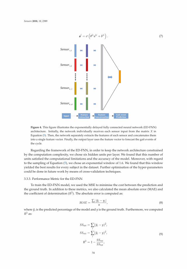
Sensors 2018, 18, 2389

al = σ(

θlcalc + blc)

. (7)

Figure 4. This figure illustrates the exponentially delayed fully connected neural network (ED-FNN)architecture. Initially, the network individually receives each sensor input from the matrix X inEquation (5). Then, the network separately extracts the features of each sensor and concatenates theminto a single feature vector. Finally, the output layer uses the feature vector to forecast the gait events ofthe cycle.

Regarding the framework of the ED-FNN, in order to keep the network architecture constrainedby the computation complexity, we chose six hidden units per layer. We found that this number ofunits satisfied the computational limitations and the accuracy of the model. Moreover, with regardto the sampling of Equation (5), we chose an exponential window of 1.6. We found that this windowyielded the best results for every subject in the dataset. Further optimisation of the hyper-parameterscould be done in future work by means of cross-validation techniques.

3.3.3. Performance Metric for the ED-FNN

To train the ED-FNN model, we used the MSE to minimise the cost between the prediction andthe ground truth. In addition to these metrics, we also calculated the mean absolute error (MAE) andthe coefficient of determination (R2). The absolute error is computed as:

MAE =∑i |yi − yi|

n, (8)

where yi is the predicted percentage of the model and y is the ground truth. Furthermore, we computedR2 as:

SStot = ∑i

(yi − y)2,

SSres = ∑i

(yi − y)2,

R2 = 1 − SSres

SStot,

(9)

54

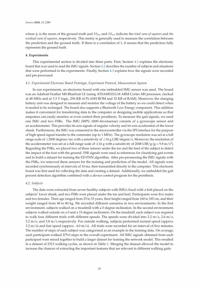
Sensors 2018, 18, 2389

where yi is the mean of the ground truth and SStot and SSres indicate the total sum of squares and the

residual sum of squares, respectively. This metric is generally used to measure the correlation betweenthe prediction and the ground truth. If there is a correlation of 1, it means that the prediction fullyrepresents the ground truth.

4. Experiments

This experimental section is divided into three parts. First, Section 4.1 explains the electronicboard that was used to read the IMU signals. Section 4.2 describes the number of subjects and situationsthat were performed in the experiments. Finally, Section 4.3 explains how the signals were recordedand pre-processed.

4.1. Experimental Electronic Board Prototype, Experiment Protocol, Measurement System

In our experiments, an electronic board with one embedded IMU sensor was used. The boardwas an Adafruit Feather M0 Bluefruit LE (using ATSAMD21G18 ARM Cortex M0 processor, clockedat 48 MHz and at 3.3 V logic, 256 KB of FLASH ROM and 32 KB of RAM). Moreover, the chargingbattery unit was designed to measure and monitor the voltage of the battery so we could detect whenit needed to be recharged. The board also supports a Bluetooth Low Energy component. This additionmakes it convenient for transferring data to the computer or designing mobile applications so thatamputees can easily monitor or even control their prosthesis. To measure the gait signals, we usedone IMU and two FSRs. The IMU (MPU 6000–Invensense) consists of a gyroscope sensor andan accelerometer. This provides tri-axis signals of angular velocity and tri-axis acceleration of the lowershank. Furthermore, the IMU was connected to the microcontroller via the SPI interface for the purposeof high-speed signal transfer to the commuter (up to 1 MHz). The gyroscope resolution was set at a fullrange scale of ±2000 degrees/sec with a sensitivity of ±16 g LSB/degree/s. Moreover, the resolution ofthe accelerometer was set at a full range scale of ±16 g with a sensitivity of 2048 LSB/g (g = 9.8 m/s2).Regarding the FSRs, we placed two of these sensors under the toe and the heel of the subject to detectthe impact of the foot with the ground. FSR signals were used as references for classifying gait eventsand to build a dataset for training the ED-FNN algorithm. After pre-prossessing the IMU signals withthe FSRs, we removed these sensors for the training and prediction of the model. All signals wererecorded synchronously at intervals of 10 ms, then transmitted directly to the computer. This electronicboard was first used for collecting the data and creating a dataset. Additionally, we embedded the gaitpercent detection algorithm combined with a device control program for the prosthesis.

4.2. Subjects

The data were extracted from seven healthy subjects with IMUs fixed with a belt placed on thesubjects’ lower shank, and two FSRs were placed under the toe and heel. Participants were five malesand two females. Their age ranged from 25 to 33 years, their height ranged from 160 to 185 cm, and theirweight ranged from 48 to 80 kg. We recorded different scenarios in two environments. In the firstenvironment, subjects walked on a treadmill with a 0 degree inclination. In the second environment,subjects walked outside on a 0 and a 15-degree inclination. On the treadmill, each subject was requiredto walk four different trials with different speeds. The speeds were divided into 2.2 m/s, 2.6 m/s,3.2 m/s, and 3.8 m/s respectively. For outside walking, subjects performed normal speed (approx.3.2 m/s) and fast speed (approx. 4.0 m/s). All trials were recorded for an interval of five minutes.The number of steps of each subject was categorised as an example in the training data. On average,each participant walked 275.0 steps in the overall experiment. All IMU signals obtained from eachparticipant were mixed together to build a larger dataset for training the network model. This resultedin a dataset of 2313 walking cycles, as shown in Table 2. Merging the dataset allowed the model toincrease the chances of extracting the important features that are relevant in different walking gaits.

55

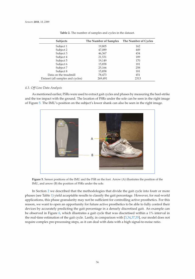
Sensors 2018, 18, 2389

Table 2. The number of samples and cycles in the dataset.

Subjects The Number of Samples The Number of Cycles

Subject 1 19,805 162Subject 2 47,089 449Subject 3 46,367 434Subject 4 21,531 189Subject 5 19,149 170Subject 6 15,858 181Subject 7 25,166 258Subject 8 15,858 181

Data on the treadmill 78,473 451Dataset (all samples and cycles) 269,491 2313

4.3. Off-Line Data Analysis

As mentioned earlier, FSRs were used to extract gait cycles and phases by measuring the heel-strikeand the toe impact with the ground. The location of FSRs under the sole can be seen in the right imageof Figure 5. The IMU’s position on the subject’s lower shank can also be seen in the right image.

A

B2

1

Figure 5. Sensor positions of the IMU and the FSR on the foot. Arrow (A) illustrates the position of theIMU, and arrow (B) the position of FSRs under the sole.

In Section 2 we described that the methodologies that divide the gait cycle into foutr or morephases (see Table 1) yield acceptable results to classify the gait percentage. However, for real-worldapplications, this phase granularity may not be sufficient for controlling active prosthetics. For thisreason, we want to open an opportunity for future active prosthetics to be able to fully control theirdevices by accurately predicting the gait percentage in a densely discretised gait. An example canbe observed in Figure 6, which illustrates a gait cycle that was discretised within a 1% interval inthe real-time estimation of the gait cycle. Lastly, in comparison with [3,34,37,55], our model does notrequire complex pre-processing steps, as it can deal with data with a high signal-to-noise ratio.

56

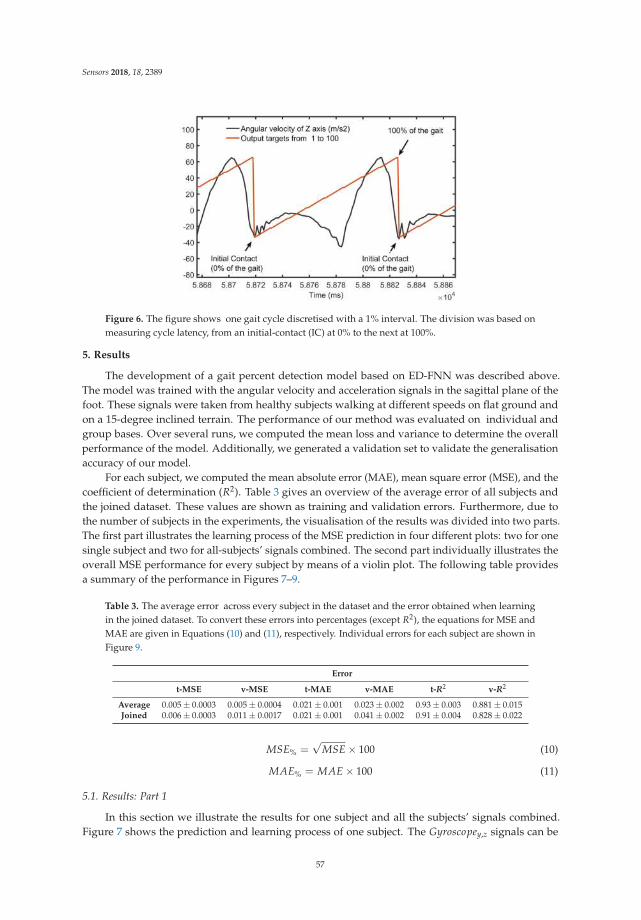
Sensors 2018, 18, 2389

Figure 6. The figure shows one gait cycle discretised with a 1% interval. The division was based onmeasuring cycle latency, from an initial-contact (IC) at 0% to the next at 100%.

5. Results

The development of a gait percent detection model based on ED-FNN was described above.The model was trained with the angular velocity and acceleration signals in the sagittal plane of thefoot. These signals were taken from healthy subjects walking at different speeds on flat ground andon a 15-degree inclined terrain. The performance of our method was evaluated on individual andgroup bases. Over several runs, we computed the mean loss and variance to determine the overallperformance of the model. Additionally, we generated a validation set to validate the generalisationaccuracy of our model.

For each subject, we computed the mean absolute error (MAE), mean square error (MSE), and thecoefficient of determination (R2). Table 3 gives an overview of the average error of all subjects andthe joined dataset. These values are shown as training and validation errors. Furthermore, due tothe number of subjects in the experiments, the visualisation of the results was divided into two parts.The first part illustrates the learning process of the MSE prediction in four different plots: two for onesingle subject and two for all-subjects’ signals combined. The second part individually illustrates theoverall MSE performance for every subject by means of a violin plot. The following table providesa summary of the performance in Figures 7–9.

Table 3. The average error across every subject in the dataset and the error obtained when learningin the joined dataset. To convert these errors into percentages (except R2), the equations for MSE andMAE are given in Equations (10) and (11), respectively. Individual errors for each subject are shown inFigure 9.

Error

t-MSE v-MSE t-MAE v-MAE t-R2 v-R2

Average 0.005 ± 0.0003 0.005 ± 0.0004 0.021 ± 0.001 0.023 ± 0.002 0.93 ± 0.003 0.881 ± 0.015Joined 0.006 ± 0.0003 0.011 ± 0.0017 0.021 ± 0.001 0.041 ± 0.002 0.91 ± 0.004 0.828 ± 0.022

MSE% =√

MSE × 100 (10)

MAE% = MAE × 100 (11)

5.1. Results: Part 1

In this section we illustrate the results for one subject and all the subjects’ signals combined.Figure 7 shows the prediction and learning process of one subject. The Gyroscopey,z signals can be

57

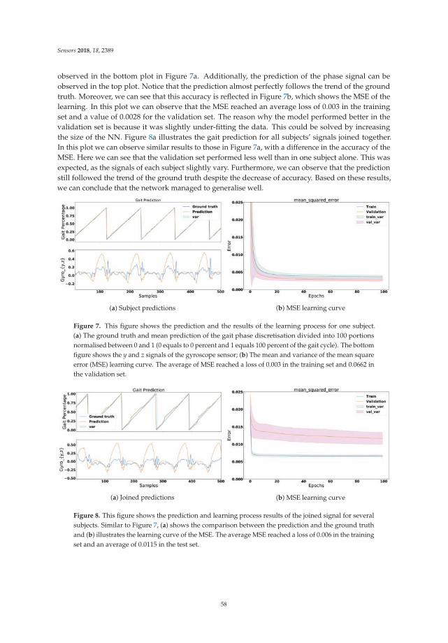
Sensors 2018, 18, 2389

observed in the bottom plot in Figure 7a. Additionally, the prediction of the phase signal can beobserved in the top plot. Notice that the prediction almost perfectly follows the trend of the groundtruth. Moreover, we can see that this accuracy is reflected in Figure 7b, which shows the MSE of thelearning. In this plot we can observe that the MSE reached an average loss of 0.003 in the trainingset and a value of 0.0028 for the validation set. The reason why the model performed better in thevalidation set is because it was slightly under-fitting the data. This could be solved by increasingthe size of the NN. Figure 8a illustrates the gait prediction for all subjects’ signals joined together.In this plot we can observe similar results to those in Figure 7a, with a difference in the accuracy of theMSE. Here we can see that the validation set performed less well than in one subject alone. This wasexpected, as the signals of each subject slightly vary. Furthermore, we can observe that the predictionstill followed the trend of the ground truth despite the decrease of accuracy. Based on these results,we can conclude that the network managed to generalise well.

(a) Subject predictions (b) MSE learning curve

Figure 7. This figure shows the prediction and the results of the learning process for one subject.(a) The ground truth and mean prediction of the gait phase discretisation divided into 100 portionsnormalised between 0 and 1 (0 equals to 0 percent and 1 equals 100 percent of the gait cycle). The bottomfigure shows the y and z signals of the gyroscope sensor; (b) The mean and variance of the mean squareerror (MSE) learning curve. The average of MSE reached a loss of 0.003 in the training set and 0.0662 inthe validation set.

(a) Joined predictions (b) MSE learning curve

Figure 8. This figure shows the prediction and learning process results of the joined signal for severalsubjects. Similar to Figure 7, (a) shows the comparison between the prediction and the ground truthand (b) illustrates the learning curve of the MSE. The average MSE reached a loss of 0.006 in the trainingset and an average of 0.0115 in the test set.

58

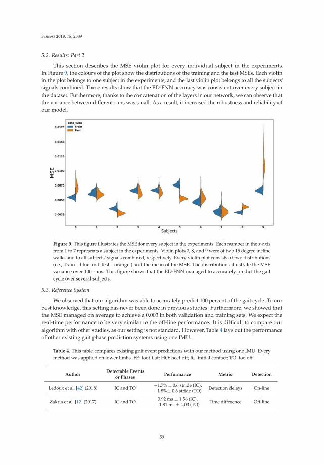
Sensors 2018, 18, 2389

5.2. Results: Part 2

This section describes the MSE violin plot for every individual subject in the experiments.In Figure 9, the colours of the plot show the distributions of the training and the test MSEs. Each violinin the plot belongs to one subject in the experiments, and the last violin plot belongs to all the subjects’signals combined. These results show that the ED-FNN accuracy was consistent over every subject inthe dataset. Furthermore, thanks to the concatenation of the layers in our network, we can observe thatthe variance between different runs was small. As a result, it increased the robustness and reliability ofour model.

Figure 9. This figure illustrates the MSE for every subject in the experiments. Each number in the x-axisfrom 1 to 7 represents a subject in the experiments. Violin plots 7, 8, and 9 were of two 15 degree inclinewalks and to all subjects’ signals combined, respectively. Every violin plot consists of two distributions(i.e., Train—blue and Test—orange ) and the mean of the MSE. The distributions illustrate the MSEvariance over 100 runs. This figure shows that the ED-FNN managed to accurately predict the gaitcycle over several subjects.

5.3. Reference System

We observed that our algorithm was able to accurately predict 100 percent of the gait cycle. To ourbest knowledge, this setting has never been done in previous studies. Furthermore, we showed thatthe MSE managed on average to achieve a 0.003 in both validation and training sets. We expect thereal-time performance to be very similar to the off-line performance. It is difficult to compare ouralgorithm with other studies, as our setting is not standard. However, Table 4 lays out the performanceof other existing gait phase prediction systems using one IMU.

Table 4. This table compares existing gait event predictions with our method using one IMU. Everymethod was applied on lower limbs. FF: foot-flat; HO: heel-off; IC: initial contact; TO: toe-off.

AuthorDetectable Events

or PhasesPerformance Metric Detection

Ledoux et al. [42] (2018) IC and TO−1.7% ± 0.6 stride (IC),−1.8%± 0.6 stride (TO)

Detection delays On-line

Zakria et al. [12] (2017) IC and TO3.92 ms ± 1.56 (IC),−1.81 ms ± 4.03 (TO)

Time difference Off-line

59

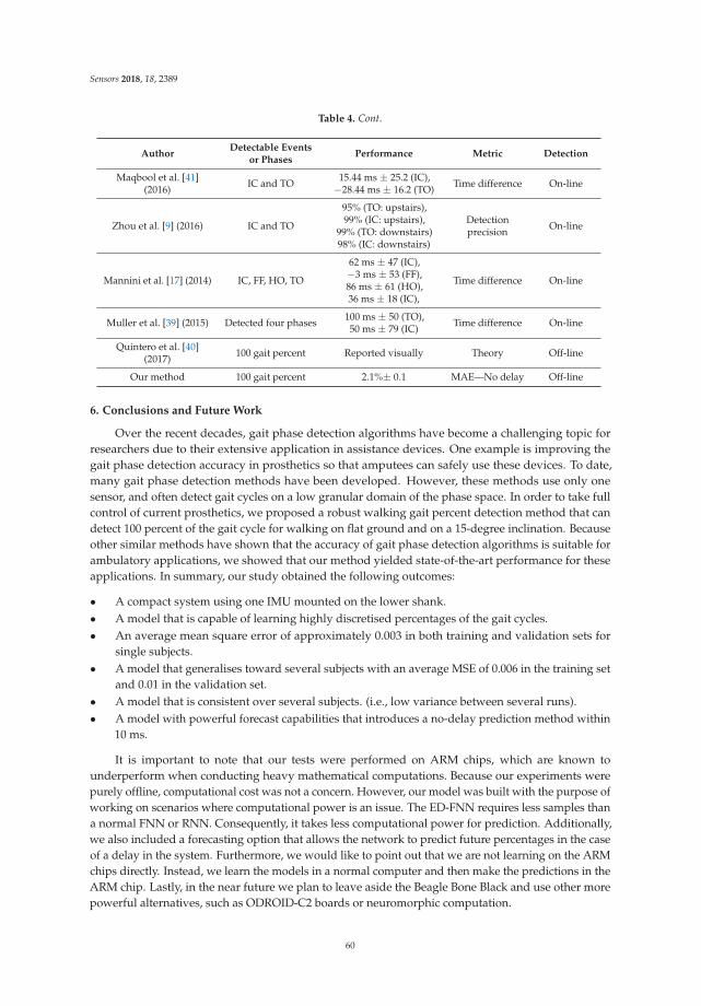
Sensors 2018, 18, 2389

Table 4. Cont.

AuthorDetectable Events

or PhasesPerformance Metric Detection

Maqbool et al. [41](2016)

IC and TO15.44 ms ± 25.2 (IC),−28.44 ms ± 16.2 (TO)

Time difference On-line

Zhou et al. [9] (2016) IC and TO

95% (TO: upstairs),99% (IC: upstairs),

99% (TO: downstairs)98% (IC: downstairs)

Detectionprecision

On-line

Mannini et al. [17] (2014) IC, FF, HO, TO

62 ms ± 47 (IC),−3 ms ± 53 (FF),86 ms ± 61 (HO),36 ms ± 18 (IC),

Time difference On-line

Muller et al. [39] (2015) Detected four phases100 ms ± 50 (TO),50 ms ± 79 (IC)

Time difference On-line

Quintero et al. [40](2017)

100 gait percent Reported visually Theory Off-line

Our method 100 gait percent 2.1%± 0.1 MAE—No delay Off-line

6. Conclusions and Future Work

Over the recent decades, gait phase detection algorithms have become a challenging topic forresearchers due to their extensive application in assistance devices. One example is improving thegait phase detection accuracy in prosthetics so that amputees can safely use these devices. To date,many gait phase detection methods have been developed. However, these methods use only onesensor, and often detect gait cycles on a low granular domain of the phase space. In order to take fullcontrol of current prosthetics, we proposed a robust walking gait percent detection method that candetect 100 percent of the gait cycle for walking on flat ground and on a 15-degree inclination. Becauseother similar methods have shown that the accuracy of gait phase detection algorithms is suitable forambulatory applications, we showed that our method yielded state-of-the-art performance for theseapplications. In summary, our study obtained the following outcomes:

• A compact system using one IMU mounted on the lower shank.• A model that is capable of learning highly discretised percentages of the gait cycles.• An average mean square error of approximately 0.003 in both training and validation sets for

single subjects.• A model that generalises toward several subjects with an average MSE of 0.006 in the training set

and 0.01 in the validation set.• A model that is consistent over several subjects. (i.e., low variance between several runs).• A model with powerful forecast capabilities that introduces a no-delay prediction method within

10 ms.

It is important to note that our tests were performed on ARM chips, which are known tounderperform when conducting heavy mathematical computations. Because our experiments werepurely offline, computational cost was not a concern. However, our model was built with the purpose ofworking on scenarios where computational power is an issue. The ED-FNN requires less samples thana normal FNN or RNN. Consequently, it takes less computational power for prediction. Additionally,we also included a forecasting option that allows the network to predict future percentages in the caseof a delay in the system. Furthermore, we would like to point out that we are not learning on the ARMchips directly. Instead, we learn the models in a normal computer and then make the predictions in theARM chip. Lastly, in the near future we plan to leave aside the Beagle Bone Black and use other morepowerful alternatives, such as ODROID-C2 boards or neuromorphic computation.

60

Sensors 2018, 18, 2389

For future work we will focus on improving the prediction accuracy and evaluation with differentwalking conditions such as stair walking and real-time implementation with the newest prosthesisversion of the AMP-Foot [4]. Additionally, the hyper-parameters of the ED-FNN model will beimproved by means of cross-validation methods.

Author Contributions: Conceptualization, F.G. and H.V.; Methodology, F.G. and H.V.; Software, F.G.; Validation,F.G. and H.V.; Formal Analysis, F.G. and H.V.; Investigation, H.V.; Resources, B.V., P.C. and D.L.; Data Curation,H.V. and F.G.; Writing—Original Draft Preparation, F.G. and H.V.; Writing—Review & Editing, F.G. and H.V.;Visualization, F.G. and H.V.; Supervision, B.V., A.N., and P.C.; Project Administration, B.V., A.N., P.C. and D.L.;Funding Acquisition, B.V. and H.V.

Funding: This research was funded by the European Commission ERC Starting grant SPEAR(No. 337596), and by the Vietnamese Government for university and college lecturers on doctoraltraining during 2010–2020 Decision of the Prime Minister No. 911/QD-TTg dated 17 June 2010.

Acknowledgments: The authors gratefully thank Timothy Verstraeten for his helpful comments and mathematicalinsights. Additionally, authors would like to express their gratitude to Astrid Van Hecke and Michal Rudz-ki forreviewing the grammar and the spelling. Finally, we would like to acknowledge the detailed assessment from theanonymous reviewers which improved the clarity and quality of the paper.

Conflicts of Interest: The authors declare no conflict of interest.

Ethical Statements: All subjects gave their informed consent for inclusion before they participated inthe study. The study was conducted in accordance with the Declaration of Helsinki, and the protocolwas approved by the Ethics Committee of B.U.N 143201526629.

References

1. Ferris, D.P.; Sawicki, G.S.; Daley, M.A. A physiologist’s perspective on robotic exoskeletons for humanlocomotion. Int. J. Humanoid Robot. 2007, 4, 507–528. [CrossRef] [PubMed]

2. Qi, Y.; Soh, C.B.; Gunawan, E.; Low, K.S.; Thomas, R. Assessment of foot trajectory for human gait phasedetection using wireless ultrasonic sensor network. IEEE Trans. Neural Syst. Rehabil. Eng. 2016, 24, 88–97.[CrossRef] [PubMed]

3. Kotiadis, D.; Hermens, H.J.; Veltink, P.H. Inertial gait phase detection for control of a drop foot stimulator.Med. Eng. Phys. 2010, 32, 287–297. [CrossRef] [PubMed]

4. Cherelle, P.; Grosu, V.; Flynn, L.; Junius, K.; Moltedo, M.; Vanderborght, B.; Lefeber, D. The Ankle MimickingProsthetic Foot 3—Locking mechanisms, actuator design, control and experiments with an amputee.Robot. Auton. Syst. 2017, 91, 327–336. [CrossRef]

5. Flynn, L.L.; Geeroms, J.; van der Hoeven, T.; Vanderborght, B.; Lefeber, D. VUB-CYBERLEGs CYBATHLON2016 Beta-Prosthesis: Case study in control of an active two degree of freedom transfemoral prosthesis.J. Neuroeng. Rehabil. 2018, 15, 3. [CrossRef] [PubMed]

6. Catalfamo, P.; Moser, D.; Ghoussayni, S.; Ewins, D. Detection of gait events using an F-Scan in-shoe pressuremeasurement system. Gait Posture 2008, 28, 420–426. [CrossRef] [PubMed]

7. Lau, H.; Tong, K. The reliability of using accelerometer and gyroscope for gait event identification on personswith dropped foot. Gait Posture 2008, 27, 248–257. [CrossRef] [PubMed]

8. Meng, X.; Yu, H.; Tham, M.P. Gait phase detection in able-bodied subjects and dementia patients.In Proceedings of the 2013 35th Annual International Conference of the IEEE Engineering in Medicineand Biology Society (EMBC), Osaka, Japan, 3–7 July 2013; pp. 4907–4910.

9. Zhou, H.; Ji, N.; Samuel, O.W.; Cao, Y.; Zhao, Z.; Chen, S.; Li, G. Towards Real-Time Detection of Gait Eventson Different Terrains Using Time-Frequency Analysis and Peak Heuristics Algorithm. Sensors 2016, 16, 1634.[CrossRef] [PubMed]

10. Khandelwal, S.; Wickström, N. Gait event detection in real-world environment for long-term applications:Incorporating domain knowledge into time-frequency analysis. IEEE Trans. Neural Syst. Rehabil. Eng. 2016,24, 1363–1372. [CrossRef] [PubMed]

11. Goršic, M.; Kamnik, R.; Ambrožic, L.; Vitiello, N.; Lefeber, D.; Pasquini, G.; Munih, M. Online phase detectionusing wearable sensors for walking with a robotic prosthesis. Sensors 2014, 14, 2776–2794. [CrossRef][PubMed]

61

Sensors 2018, 18, 2389

12. Zakria, M.; Maqbool, H.F.; Hussain, T.; Awad, M.I.; Mehryar, P.; Iqbal, N.; Dehghani-Sanij, A.A.Heuristic based gait event detection for human lower limb movement. In Proceedings of the 2017 IEEE EMBSInternational Conference on Biomedical & Health Informatics (BHI), Jeju Island, Korea, 11–15 July 2017;pp. 337–340.

13. Mannini, A.; Sabatini, A.M. Machine learning methods for classifying human physical activity from on-bodyaccelerometers. Sensors 2010, 10, 1154–1175. [CrossRef] [PubMed]

14. Bae, J.; Tomizuka, M. Gait phase analysis based on a Hidden Markov Model. Mechatronics 2011, 21, 961–970.[CrossRef]

15. Mannini, A.; Sabatini, A.M. A hidden Markov model-based technique for gait segmentation usinga foot-mounted gyroscope. In Proceedings of the 2011 Annual International Conference of the IEEEEngineering in Medicine and Biology Society (EMBC), Boston, MA, USA, 30 August–3 September 2011;pp. 4369–4373.

16. Crea, S.; De Rossi, S.M.; Donati, M.; Reberšek, P.; Novak, D.; Vitiello, N.; Lenzi, T.; Podobnik, J.; Munih, M.;Carrozza, M.C. Development of gait segmentation methods for wearable foot pressure sensors. In Proceedingsof the 2012 Annual International Conference of the IEEE Engineering in Medicine and Biology Society (EMBC),San Diego, CA, USA, 28 August–1 September 2012; pp. 5018–5021.

17. Mannini, A.; Genovese, V.; Sabatini, A.M. Online decoding of hidden Markov models for gait event detectionusing foot-mounted gyroscopes. IEEE J. Biomed. Health Inf. 2014, 18, 1122–1130. [CrossRef] [PubMed]

18. Taborri, J.; Scalona, E.; Rossi, S.; Palermo, E.; Patanè, F.; Cappa, P. Real-time gait detection based on HiddenMarkov Model: is it possible to avoid training procedure? In Proceedings of the 2015 IEEE InternationalSymposium on Medical Measurements and Applications (MeMeA), Torino, Italy, 7–9 May 2015; pp. 141–145.

19. Taborri, J.; Scalona, E.; Palermo, E.; Rossi, S.; Cappa, P. Validation of inter-subject training for hiddenMarkov models applied to gait phase detection in children with cerebral palsy. Sensors 2015, 15, 24514–24529.[CrossRef] [PubMed]

20. Liu, D.X.; Wu, X.; Du, W.; Wang, C.; Xu, T. Gait phase recognition for lower-limb exoskeleton with only jointangular sensors. Sensors 2016, 16, 1579. [CrossRef] [PubMed]

21. Tanghe, K.; Harutyunyan, A.; Aertbeliën, E.; De Groote, F.; De Schutter, J.; Vrancx, P.; Nowé, A.Predicting seat-off and detecting start-of-assistance events for assisting sit-to-stand with an exoskeleton.IEEE Robot. Autom. Lett. 2016, 1, 792–799. [CrossRef]

22. Gouwanda, D.; Gopalai, A.A. A robust real-time gait event detection using wireless gyroscope and itsapplication on normal and altered gaits. Med. Eng. Phys. 2015, 37, 219–225. [CrossRef] [PubMed]

23. Evans, R.L.; Arvind, D. Detection of gait phases using orient specks for mobile clinical gait analysis.In Proceedings of the 2014 11th International Conference on Wearable and Implantable Body SensorNetworks (BSN), Zurich, Switzerland, 16–19 June 2014; pp. 149–154.

24. Agostini, V.; Balestra, G.; Knaflitz, M. Segmentation and classification of gait cycles. IEEE Trans. Neural Syst.

Rehabil. Eng. 2014, 22, 946–952. [CrossRef] [PubMed]25. Skelly, M.M.; Chizeck, H.J. Real-time gait event detection for paraplegic FES walking. IEEE Trans. Neural Syst.

Rehabil. Eng. 2001, 9, 59–68. [CrossRef] [PubMed]26. De Rossi, S.M.; Crea, S.; Donati, M.; Reberšek, P.; Novak, D.; Vitiello, N.; Lenzi, T.; Podobnik, J.; Munih, M.;

Carrozza, M.C. Gait segmentation using bipedal foot pressure patterns. In Proceedings of the 2012 4th IEEERAS & EMBS International Conference on Biomedical Robotics and Biomechatronics (BioRob), Rome, Italy,24–27 June 2012; pp. 361–366.

27. Cherelle, P.; Grosu, V.; Matthys, A.; Vanderborght, B.; Lefeber, D. Design and validation of the anklemimicking prosthetic (AMP-) foot 2.0. IEEE Trans. Neural Syst. Rehabil. Eng. 2014, 22, 138–148. [CrossRef][PubMed]

28. Moulianitis, V.C.; Syrimpeis, V.N.; Aspragathos, N.A.; Panagiotopoulos, E.C. A closed-loop drop-footcorrection system with gait event detection from the contralateral lower limb using fuzzy logic. In Proceedingsof the 2011 10th International Workshop on Biomedical Engineering, Kos, Greece, 5–7 October 2011; pp. 1–4.

29. Joshi, C.D.; Lahiri, U.; Thakor, N.V. Classification of gait phases from lower limb EMG: Applicationto exoskeleton orthosis. In Proceedings of the 2013 IEEE Point-of-Care Healthcare Technologies (PHT),Bangalore, India, 16–18 January 2013; pp. 228–231.

62

Sensors 2018, 18, 2389

30. Mannini, A.; Trojaniello, D.; Cereatti, A.; Sabatini, A.M. A machine learning framework for gait classificationusing inertial sensors: Application to elderly, post-stroke and huntington’s disease patients. Sensors 2016, 16, 134.[CrossRef] [PubMed]

31. Patterson, M.; Caulfield, B. A novel approach for assessing gait using foot mounted accelerometers.In Proceedings of the 2011 5th International Conference on Pervasive Computing Technologies for Healthcare(PervasiveHealth), Dublin, Ireland, 23–26 May 2011; pp. 218–221.

32. Zheng, E.; Wang, Q. Noncontact capacitive sensing-based locomotion transition recognition for amputeeswith robotic transtibial prostheses. IEEE Trans. Neural Syst. Rehabil. Eng. 2017, 25, 161–170. [CrossRef][PubMed]

33. Zhao, Y.; Zhou, S. Wearable device-based gait recognition using angle embedded gait dynamic images anda convolutional neural network. Sensors 2017, 17, 478. [CrossRef] [PubMed]

34. Maqbool, H.F.; Husman, M.A.B.; Awad, M.I.; Abouhossein, A.; Iqbal, N.; Dehghani-Sanij, A.A. A real-timegait event detection for lower limb prosthesis control and evaluation. IEEE Trans. Neural Syst. Rehabil. Eng.

2017, 25, 1500–1509. [CrossRef] [PubMed]35. Taborri, J.; Palermo, E.; Rossi, S.; Cappa, P. Gait partitioning methods: A systematic review. Sensors 2016, 16, 66.

[CrossRef] [PubMed]36. Neumann, D.A. Kinesiology of the Musculoskeletal System: Foundations for Physical Rehabilitation; Mosby:

St. Louis, MO, USA, 2002.37. Boutaayamou, M.; Schwartz, C.; Stamatakis, J.; Denoël, V.; Maquet, D.; Forthomme, B.; Croisier, J.L.; Macq, B.;

Verly, J.G.; Garraux, G.; et al. Development and validation of an accelerometer-based method for quantifyinggait events. Med. Eng. Phys. 2015, 37, 226–232. [CrossRef] [PubMed]

38. Rueterbories, J.; Spaich, E.G.; Andersen, O.K. Gait event detection for use in FES rehabilitation by radial andtangential foot accelerations. Med. Eng. Phys. 2014, 36, 502–508. [CrossRef] [PubMed]

39. Muller, P.; Steel, T.; Schauer, T. Experimental evaluation of a novel inertial sensor based realtime gait phasedetection algorithm. In Proceedings of the Technically Assisted Rehabilitation Conference, Berlin, Germany,12 March 2015.

40. Quintero, D.; Lambert, D.J.; Villarreal, D.J.; Gregg, R.D. Real-time continuous gait phase and speed estimationfrom a single sensor. In Proceedings of the 2017 IEEE Conference on Control Technology and Applications(CCTA), Mauna Lani, HI, USA, 27–30 August 2017; pp. 847–852.

41. Maqbool, H.F.; Husman, M.A.B.; Awad, M.I.; Abouhossein, A.; Mehryar, P.; Iqbal, N.; Dehghani-Sanij, A.A.Real-time gait event detection for lower limb amputees using a single wearable sensor. In Proceedings ofthe 2016 IEEE 38th Annual International Conference of the Engineering in Medicine and Biology Society(EMBC), Orlando, FL, USA, 16–20 August 2016; pp. 5067–5070.

42. Ledoux, E. Inertial Sensing for Gait Event Detection and Transfemoral Prosthesis Control Strategy. IEEE Trans.

Biomed. Eng. 2018. [CrossRef] [PubMed]43. Shorter, K.A.; Polk, J.D.; Rosengren, K.S.; Hsiao-Wecksler, E.T. A new approach to detecting asymmetries in

gait. Clin. Biomech. 2008, 23, 459–467. [CrossRef] [PubMed]44. Fisher, R.A. The use of multiple measurements in taxonomic problems. Ann. Hum. Genet. 1936, 7, 179–188.

[CrossRef]45. Ito, Y. Representation of functions by superpositions of a step or sigmoid function and their applications to

neural network theory. Neural Netw. 1991, 4, 385–394. [CrossRef]46. Duan, K.; Keerthi, S.S.; Chu, W.; Shevade, S.K.; Poo, A.N. Multi-category classification by soft-max

combination of binary classifiers. In Proceedings of the International Workshop on Multiple ClassifierSystems, Guildford, UK, 11–13 June 2003; Springer: Berlin, Germany, 2003; pp. 125–134.

47. Nair, V.; Hinton, G.E. Rectified linear units improve restricted boltzmann machines. In Proceedings of the27th International Conference on Machine Learning (ICML-10), Haifa, Israel, 21–24 June 2010; pp. 807–814.

48. Allen, D.M. Mean square error of prediction as a criterion for selecting variables. Technometrics 1971,13, 469–475. [CrossRef]

49. Shore, J.; Johnson, R. Axiomatic derivation of the principle of maximum entropy and the principle ofminimum cross-entropy. IEEE Trans. Inf. Theory 1980, 26, 26–37. [CrossRef]

50. Bottou, L. Large-scale machine learning with stochastic gradient descent. In Proceedings of the 19thInternational Symposium on Computational Statistics (COMPSTAT’2010), Paris, France, 22–27 August 2010;Springer: Berlin, Germany, 2010; pp. 177–186.

63

Sensors 2018, 18, 2389

51. Møller, M.F. A scaled conjugate gradient algorithm for fast supervised learning. Neural Netw. 1993, 6, 525–533.[CrossRef]

52. Kingma, D.P.; Ba, J. Adam: A method for stochastic optimization. arXiv 2014, arXiv:1412.6980.53. LeCun, Y.; Bengio, Y.; Hinton, G. Deep learning. Nature 2015, 521, 436. [CrossRef] [PubMed]54. Gers, F.A.; Schmidhuber, J.; Cummins, F. Learning to Forget: Continual Prediction with LSTM. In Proceedings

of the 9th International Conference on Artificial Neural Networks (ICANN ’99), San Sebastián, Spain,20–22 June 2007; pp. 850–855.

55. Wang, Q.; Yuan, K.; Zhu, J.; Wang, L. Walk the walk: A lightweight active transtibial prosthesis. IEEE Robot.

Autom. Mag. 2015, 22, 80–89. [CrossRef]

c© 2018 by the authors. Licensee MDPI, Basel, Switzerland. This article is an open accessarticle distributed under the terms and conditions of the Creative Commons Attribution(CC BY) license (http://creativecommons.org/licenses/by/4.0/).

64

sensors

Article

A Vision-Driven Collaborative Robotic GraspingSystem Tele-Operated by Surface Electromyography

Andrés Úbeda 1,2, Brayan S. Zapata-Impata 1,2, Santiago T. Puente 1,2, Pablo Gil 1,2,

Francisco Candelas 1,2 and Fernando Torres 1,2,*

1 Department of Physics, System Engineering and Signal Theory, University of Alicante, 03690 Alicante, Spain;andres.ubeda@ua.es (A.Ú.); brayan.impata@ua.es (B.S.Z.-I.); santiago.puente@ua.es (S.T.P.);pablo.gil@ua.es (P.G.); Francisco.Candelas@ua.es (F.C.)

2 Computer Science Research Institute, University of Alicante, 03690 Alicante, Spain* Correspondence: fernando.torres@ua.es; Tel.: +34-965-90-9491

Received: 27 June 2018; Accepted: 16 July 2018; Published: 20 July 2018

Abstract: This paper presents a system that combines computer vision and surface electromyographytechniques to perform grasping tasks with a robotic hand. In order to achieve a reliable graspingaction, the vision-driven system is used to compute pre-grasping poses of the robotic system based onthe analysis of tridimensional object features. Then, the human operator can correct the pre-graspingpose of the robot using surface electromyographic signals from the forearm during wrist flexion andextension. Weak wrist flexions and extensions allow a fine adjustment of the robotic system to graspthe object and finally, when the operator considers that the grasping position is optimal, a strongflexion is performed to initiate the grasping of the object. The system has been tested with severalsubjects to check its performance showing a grasping accuracy of around 95% of the attemptedgrasps which increases in more than a 13% the grasping accuracy of previous experiments in whichelectromyographic control was not implemented.

Keywords: surface electromyography; computer vision; grasping; assistive robotics

1. Introduction

Nowadays, robots can perform a variety of tasks to help human operators in their work [1]. The useof robots to collaborate with people with disabilities in industrial environments is a growing sector.For instance, several studies analyse the execution of manufacturing tasks by disabled people [2,3].In this line, robotic assistive technologies have been successfully introduced following two differentapproaches. They are used to assist humans who have motor disabilities to perform daily activities.Typical examples are prosthetics devices and exoskeletons for motor substitution, or smart homes wherehousehold tasks are performed and controlled by automatic systems. These technologies also providenovel rehabilitation therapies to recover motor function and reduce further complications. Essentially,assistive technologies seek to improve the well-being of humans with disabilities [4].

The inclusion of assistive robotics in industrial applications contributes to the improvement ofoccupational health of human operators. Tele-operation systems increase the degree of assistancein dangerous manipulation tasks. Their goal is to make a system capable of mimicking and scalingthe movements of a human operator in the control of a manipulator avoiding the risks of handlingdangerous products or carrying out dangerous actions. Before including assistive technologies inindustrial tasks, several teleoperation aspects must be considered. One of them is the feedback to theuser, therefore the use of haptic interfaces [5] is critical to obtain a more natural feeling of the robotoperation. Another important aspect is the additional assistance given to the user in the performance ofthe assigned task; focused, for instance, on the possibility of providing an amputee with the capability

Sensors 2018, 18, 2366; doi:10.3390/s18072366 www.mdpi.com/journal/sensors65

Sensors 2018, 18, 2366

of performing bimanual tasks [6]. The need of interacting with the environment requires of visionsystems to recognise the working place and provide a proper manipulation of the products [7].

A good option to achieve a proper tele-operated robotic manipulation is to implementsolutions based on techniques that provide reliable control signals from the human operator. Surfaceelectromyography (sEMG) allows a system to record the electrical activity of muscle contractions ina non-invasive way [8]. The use of this information to control external devices is called myocontrol.Myocontrol techniques have been usually developed to obtain a reliable actuation of assistive devicesin the field of prosthetics. This actuation ranges from simple binary control commands to complexmultidimensional control [9,10].

Complex techniques have been applied to multi-finger prosthetic devices and robotic hands.However, myocontrol is generally limited to a few hand grips and still unreliable in realisticenvironments [11]. To avoid these limitations, several approaches have been recently proposed.One option is to provide a proper sensory feedback to the subject to close the control loop [12,13].However, this option is still limited to the low accuracy in the classification of complex biomechanicaltasks. Another alternative is the introduction of multimodal control of the robotic actuation whichmay provide a good solution to the unreliability of multidimensional control. In this case, anothercontrol method, such as gaze-tracking or electrooculography, is combined with myocontrol to increasereliability and speed [14,15]. Its main disadvantage is the increased workload on the user as bothinteraction methods must be controlled simultaneously.

To solve the problems arisen from the previously described solutions, we propose the use ofa shared control of the end effector of the robot arm. To achieve this, complex positioning and graspingtasks are performed by an alternative system and sEMG processing provides high-level commands.In this case, myocontrol will be combined with a vision-based grasping system.

Grasping is one of the most significant tasks which is performed by humans in everyday manipulationprocesses. In recent works, robots have been provided with the ability to grasp objects [16,17]. It isoften possible to see robots autonomously grasping objects in many industrial applications in which theenvironment is not dynamic and where both geometry and pose of objects are known. Therefore, theproper pose of the robotic hand or gripper to grasp the object is computed only once. This process isrepeated whenever it is needed. More recently, robots are beginning to be self-sufficient and they arereaching a great level of autonomy to work without human intervention in unstructured scenarios or withdynamics in which the kind of objects or their poses are unknown, for example in industrial applicationsas in [18] and in storage and logistic applications [19].

Many grasp methods have been made possible by the advances in visual perception techniquesof the environment, both 2D [20] and 3D [21]. In general, both techniques combine computer visionalgorithms and traditional machine learning, the first for the extraction of object features of the sceneand the second for the recognition of the objects by comparison and classification of extracted featureswith features from a dataset of known objects. Thereby, visual perception has allowed robots to havethe ability of grasping in a similar way to humans, though under certain conditions, making use ofobject recognition algorithms [22–24] and pose estimation algorithms [25,26]. Recently, a significantnumber of new approaches have been proposed to localize robotic grasp configurations directly fromsensor data without estimating object pose using training databases of real objects [27] or syntheticobjects (CAD models) as in [28].

However, currently it is still not possible to compare the ability of robots and humans to graspobjects in a generic way, for each and every situation. The main drawback of applying visual perceptiontechniques to accomplish a completely autonomous grasping is the great variability of the kind ofobjects (geometric shape, pose and visual appearance such as color or texture) that can be present inan environment. This demands a large datasets of training data to implement a robust algorithm toavoid ambiguity in both recognition and location processes of the objects in the scene. The proposedsystem may solve both the more relevant issues of grasping and the complexity of multidimensional

66

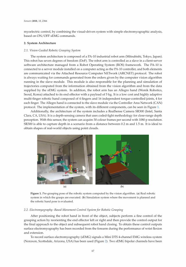
Sensors 2018, 18, 2366

myoelectric control, by combining the visual-driven system with simple electromyographic analysis,based on ON/OFF sEMG commands.

2. System Architecture

2.1. Vision-Guided Robotic Grasping System

The system architecture is composed of a PA-10 industrial robot arm (Mitsubishi, Tokyo, Japan).This robot has seven degrees of freedom (DoF). The robot arm is controlled as a slave in a client-serversoftware architecture managed from a Robot Operating System (ROS) framework. The PA-10 isconnected to a server module installed on a computer acting as the PA-10 controller, and both elementsare communicated via the Attached Resource Computer NETwork (ARCNET) protocol. The robotis always waiting for commands generated from the orders given by the computer vision algorithmrunning in the slave module. This module is also responsible for the planning and simulation oftrajectories computed from the information obtained from the vision algorithm and from the datasupplied by the sEMG system. In addition, the robot arm has an Allegro hand (Wonik Robotics,Seoul, Korea) attached to its end effector with a payload of 5 kg. It is a low cost and highly adaptivemulti-finger robotic hand composed of 4 fingers and 16 independent torque-controlled joints, 4 foreach finger. The Allegro hand is connected to the slave module via the Controller Area Network (CAN)protocol. The implementation of the system, with its different components, can be seen in Figure 1.

Additionally, the architecture of the system includes a RealSense Camera SR300 (Intel, SantaClara, CA, USA). It is a depth-sensing camera that uses coded-light methodology for close-range depthperception. With this sensor, the system can acquire 30 colour frames per second with 1080 p resolution.SR300 is able to capture depth in a scenario from a distance between 0.2 m and 1.5 m. It is ideal toobtain shapes of real-world objects using point clouds.

(a) (b)

Figure 1. Pre-grasping pose of the robotic system computed by the vision algorithm. (a) Real roboticsystem in which the grasps are executed. (b) Simulation system where the movement is planned andthe robotic hand pose is evaluated.

2.2. Electromyography -Based Movement Control System for Robotic Grasping

After positioning the robot hand in front of the object, subjects perform a fine control of thegrasping action by reorienting the end effector left or right and then provide the control output forthe final approach to the object and subsequent robot hand closing. To obtain these control outputssurface electromyography has been recorded from the forearm during the performance of wrist flexionand extension.

To record surface electromyography (sEMG) signals a Mini DTS 4-channel EMG wireless system(Noraxon, Scottsdale, Arizona, USA) has been used (Figure 2). Two sEMG bipolar channels have been

67

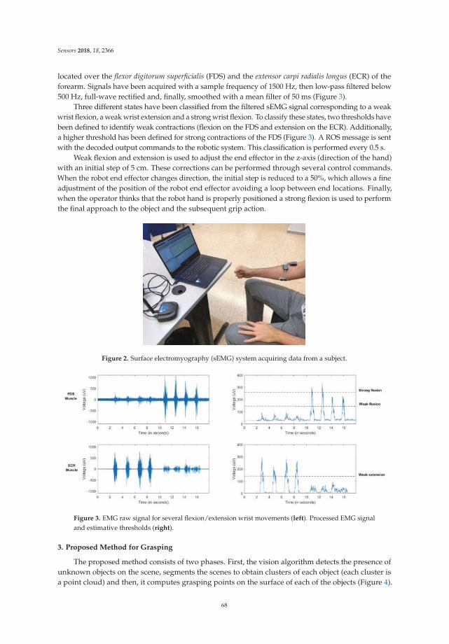
Sensors 2018, 18, 2366

located over the flexor digitorum superficialis (FDS) and the extensor carpi radialis longus (ECR) of theforearm. Signals have been acquired with a sample frequency of 1500 Hz, then low-pass filtered below500 Hz, full-wave rectified and, finally, smoothed with a mean filter of 50 ms (Figure 3).

Three different states have been classified from the filtered sEMG signal corresponding to a weakwrist flexion, a weak wrist extension and a strong wrist flexion. To classify these states, two thresholds havebeen defined to identify weak contractions (flexion on the FDS and extension on the ECR). Additionally,a higher threshold has been defined for strong contractions of the FDS (Figure 3). A ROS message is sentwith the decoded output commands to the robotic system. This classification is performed every 0.5 s.

Weak flexion and extension is used to adjust the end effector in the z-axis (direction of the hand)with an initial step of 5 cm. These corrections can be performed through several control commands.When the robot end effector changes direction, the initial step is reduced to a 50%, which allows a fineadjustment of the position of the robot end effector avoiding a loop between end locations. Finally,when the operator thinks that the robot hand is properly positioned a strong flexion is used to performthe final approach to the object and the subsequent grip action.

Figure 2. Surface electromyography (sEMG) system acquiring data from a subject.

Figure 3. EMG raw signal for several flexion/extension wrist movements (left). Processed EMG signaland estimative thresholds (right).

3. Proposed Method for Grasping

The proposed method consists of two phases. First, the vision algorithm detects the presence ofunknown objects on the scene, segments the scenes to obtain clusters of each object (each cluster isa point cloud) and then, it computes grasping points on the surface of each of the objects (Figure 4).

68

Sensors 2018, 18, 2366

The method is flexible to obtain grasping points of objects even changing the scenario providing thatobjects are located on a table or flat surface. Once the vision algorithm provides the robot with theoptimal grasping points of the object, the robot plans the trajectory in order to position the robot handto grasp the object. Occasionally, the grasping of the object is not optimal. For this reason, the methodadds a second phase which is used to plan fine hand robot-object interactions. In this step, EMG-basedteleoperation of the robot hand-arm is performed to accomplish a successful and stable grasp withoutslipping and avoiding damage to the object.

3.1. Grasping Points and Pose Estimation

The algorithm calculates pairs of contact points for unknown objects given a single point cloudcaptured from a RGBD sensor with eye-to-hand configuration. Firstly, the point cloud is segmented inorder to detect the objects present in the scene. Then, for each detected object, the algorithm evaluatespairs of contact points that fulfil a set of geometric conditions. Basically, it approximates the mainaxis of the object using the major vector obtained by running a Principal Component Analysis (PCA)extraction. Then, it calculates the centroid in the point cloud. With this information, it is possible tofind a cutting plane perpendicular to the main axis of the object through its centroid. The candidatecontact areas are at the opposite edges of the surface of the object that are close to the cutting plane.A standard grasping configuration consists of one point from each of these two areas. Figure 4 showsall these steps graphically.

These candidate areas, in which the robot hand can be positioned, contain multiple potentialpoints so the vision algorithm evaluates a great variety of grasping configurations for the robot hand,using a custom metric that ranks their feasibility. Thereby, the best-ranked pair of contact pointsis selected, since it is likely to be the most stable grasp, given the view conditions and the usedrobotic hand. The algorithm takes into account four aspects: the distance of the contact points tothe cutting plane, the geometric curvature at the contact points, the antipodal configurations and theperpendicularity to the contact points.

Figure 4. Steps of the method for calculating a pair of contact points. Scene Segmentation: clouds of thedetected objects. Grasping Points Calculus, executed for each detected object: (1) grasping areas withpotential contact points, (2) curvature values and a pair of evaluated contact points, (3) best rankedpair of contact points.

69

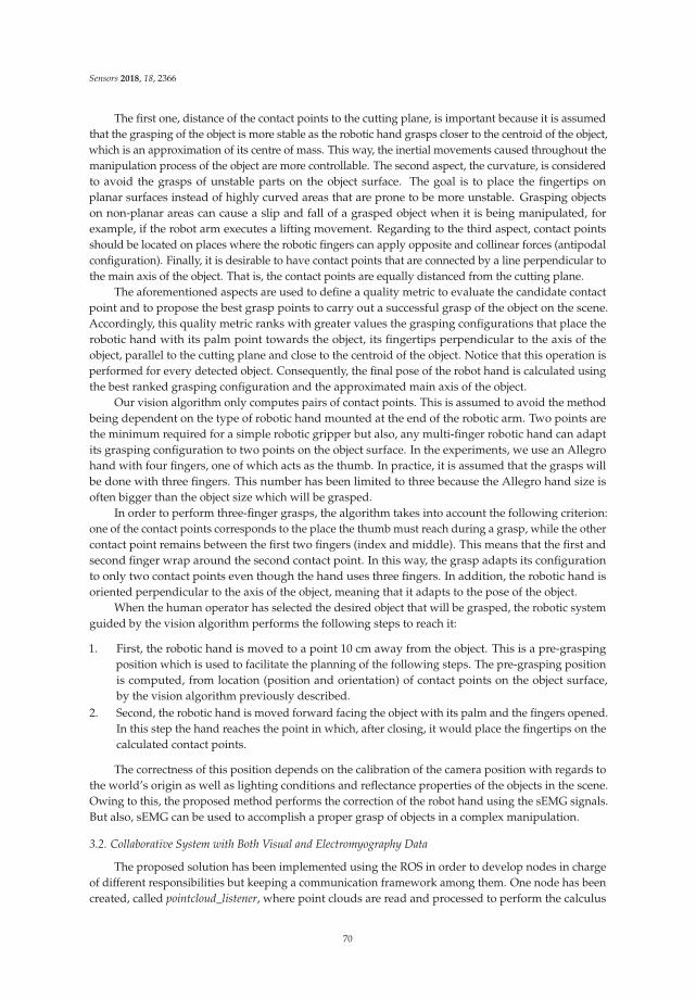
Sensors 2018, 18, 2366

The first one, distance of the contact points to the cutting plane, is important because it is assumedthat the grasping of the object is more stable as the robotic hand grasps closer to the centroid of the object,which is an approximation of its centre of mass. This way, the inertial movements caused throughout themanipulation process of the object are more controllable. The second aspect, the curvature, is consideredto avoid the grasps of unstable parts on the object surface. The goal is to place the fingertips onplanar surfaces instead of highly curved areas that are prone to be more unstable. Grasping objectson non-planar areas can cause a slip and fall of a grasped object when it is being manipulated, forexample, if the robot arm executes a lifting movement. Regarding to the third aspect, contact pointsshould be located on places where the robotic fingers can apply opposite and collinear forces (antipodalconfiguration). Finally, it is desirable to have contact points that are connected by a line perpendicular tothe main axis of the object. That is, the contact points are equally distanced from the cutting plane.

The aforementioned aspects are used to define a quality metric to evaluate the candidate contactpoint and to propose the best grasp points to carry out a successful grasp of the object on the scene.Accordingly, this quality metric ranks with greater values the grasping configurations that place therobotic hand with its palm point towards the object, its fingertips perpendicular to the axis of theobject, parallel to the cutting plane and close to the centroid of the object. Notice that this operation isperformed for every detected object. Consequently, the final pose of the robot hand is calculated usingthe best ranked grasping configuration and the approximated main axis of the object.

Our vision algorithm only computes pairs of contact points. This is assumed to avoid the methodbeing dependent on the type of robotic hand mounted at the end of the robotic arm. Two points arethe minimum required for a simple robotic gripper but also, any multi-finger robotic hand can adaptits grasping configuration to two points on the object surface. In the experiments, we use an Allegrohand with four fingers, one of which acts as the thumb. In practice, it is assumed that the grasps willbe done with three fingers. This number has been limited to three because the Allegro hand size isoften bigger than the object size which will be grasped.

In order to perform three-finger grasps, the algorithm takes into account the following criterion:one of the contact points corresponds to the place the thumb must reach during a grasp, while the othercontact point remains between the first two fingers (index and middle). This means that the first andsecond finger wrap around the second contact point. In this way, the grasp adapts its configurationto only two contact points even though the hand uses three fingers. In addition, the robotic hand isoriented perpendicular to the axis of the object, meaning that it adapts to the pose of the object.

When the human operator has selected the desired object that will be grasped, the robotic systemguided by the vision algorithm performs the following steps to reach it:

1. First, the robotic hand is moved to a point 10 cm away from the object. This is a pre-graspingposition which is used to facilitate the planning of the following steps. The pre-grasping positionis computed, from location (position and orientation) of contact points on the object surface,by the vision algorithm previously described.

2. Second, the robotic hand is moved forward facing the object with its palm and the fingers opened.In this step the hand reaches the point in which, after closing, it would place the fingertips on thecalculated contact points.

The correctness of this position depends on the calibration of the camera position with regards tothe world’s origin as well as lighting conditions and reflectance properties of the objects in the scene.Owing to this, the proposed method performs the correction of the robot hand using the sEMG signals.But also, sEMG can be used to accomplish a proper grasp of objects in a complex manipulation.

3.2. Collaborative System with Both Visual and Electromyography Data

The proposed solution has been implemented using the ROS in order to develop nodes in chargeof different responsibilities but keeping a communication framework among them. One node has beencreated, called pointcloud_listener, where point clouds are read and processed to perform the calculus

70

Sensors 2018, 18, 2366

of the grasp contacts. This node publishes a custom ROS message called GraspConfiguration where thepoint clouds of the objects and the calculated grasp contacts are stored.

Another node, called allegro_control_grasp, subscribes to this topic and reads the published contactpoints to generate a grasp pose for the robotic gripper. Then, it proceeds to plan a trajectory followingthe steps listed in the previous section. MoveIt! [29] has been used to perform this trajectory planning.Once it reaches the grasping position, the EMG control starts. To do so, it subscribes to a topiccalled/emgsensor/move where the correcting movements are published.

These corrections are published by a third node called emg_reader, which processes the sEMGsignals in order to provide messages of type geometry_msgs/Quaternion. This type of ROS messageallows us to describe the direction of movement for the arm that the operator wants to perform inorder to correct the position of the robotic gripper. Thus, using one of the axis of the Quaternion,we can specify in which axis we want to move the gripper. The w term is set to 1 when we detect thegrasping pattern in the EMG signal so the allegro_control_grasp node closes the gripper and continuesto lift and carry the object.

It is important to note that this message is constantly published by the emg_reader node butthe allegro_control_grasp only reads them after performing a correction. This means that messagespublished during the physical movement of the robot are ignored and, as soon as it stops, the controlreturns to wait for a new message in the topic. Figure 5 shows a scheme of the nodes and theirinteractions through ROS.

Figure 5. Scheme of the proposed method implemented in Robot Operating System (ROS) showingcommunication modules among different steps.

4. Experiments and Discussion

4.1. Test Design

Six subjects (age 24.5 ± 6.2 years old, four male and two female) without previous experienceon myoelectric control participated in the experimental tests. First, subjects were asked to performseveral wrist flexion and extensions at different force levels and thresholds were visually chosen fromthe processed sEMG signals of the FDS and ECR. After selecting the proper thresholds, subjects wereasked to freely perform wrist contractions and the classification output was shown to them until theyfelt comfortable with the myoelectric setup.

The experimental tests were divided into three sets of grasping activities, each one for a differentpositioning of the object. The object, a cylindrical plastic can (23 cm height, 8 cm diameter), wasplaced vertically (position 1), horizontally (position 2) and in a diagonal orientation (position 3). Each

71

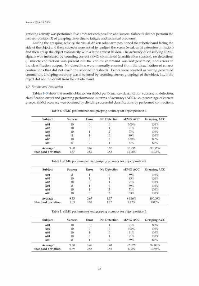
Sensors 2018, 18, 2366

grasping activity was performed five times for each position and subject. Subject 5 did not perform thelast set (position 3) of grasping tasks due to fatigue and technical problems.

During the grasping activity, the visual-driven robot arm positioned the robotic hand facing theside of the object and then, subjects were asked to readjust the z-axis (weak wrist extension or flexion)and then grasp the object voluntarily with a strong wrist flexion. The accuracy of classifying sEMGsignals was measured by counting correct sEMG commands (classification success), no detections(if muscle contraction was present but the control command was not generated) and errors inthe classification output. No detections were manually counted from the visualization of correctcontractions that did not reach the selected thresholds. Errors were counted as wrong generatedcommands. Grasping accuracy was measured by counting correct graspings of the object, i.e., if theobject did not flip or fall from the robotic hand.

4.2. Results and Evaluation

Tables 1–3 show the results obtained on sEMG performance (classification success, no detection,classification error) and grasping performance in terms of accuracy (ACC), i.e., percentage of correctgrasps. sEMG accuracy was obtained by dividing successful classifications by performed contractions.

Table 1. sEMG performance and grasping accuracy for object position 1.

Subject Success Error No Detection sEMG ACC Grasping ACC

A01 10 0 0 100% 100%A02 10 0 1 91% 100%A03 10 1 2 77% 100%A04 8 1 0 89% 100%A05 10 0 0 100% 80%A06 6 2 1 67% 80%

Average 9.00 0.67 0.67 87.23% 93.33%Standard deviation 1.67 0.82 0.82 13.20% 10.33%

Table 2. sEMG performance and grasping accuracy for object position 2.

Subject Success Error No Detection sEMG ACC Grasping ACC

A01 8 1 0 89% 100%A02 10 1 1 83% 100%A03 10 0 1 91% 100%A04 8 1 0 89% 100%A05 10 1 3 71% 100%A06 10 0 2 83% 100%

Average 9.33 0.67 1.17 84.46% 100.00%Standard deviation 1.03 0.52 1.17 7.12% 0.00%

Table 3. sEMG performance and grasping accuracy for object position 3.

Subject Success Error No Detection sEMG ACC Grasping ACC

A01 10 0 1 91% 80%A02 10 0 0 100% 100%A03 10 1 0 91% 100%A04 10 0 1 91% 100%A06 8 1 0 89% 80%

Average 9.60 0.40 0.40 92.32% 92.00%Standard deviation 0.89 0.55 0.55 4.38% 10.95%

72

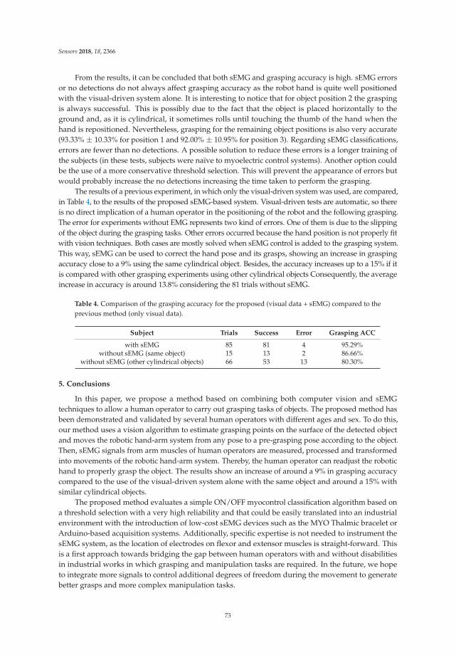
Sensors 2018, 18, 2366

From the results, it can be concluded that both sEMG and grasping accuracy is high. sEMG errorsor no detections do not always affect grasping accuracy as the robot hand is quite well positionedwith the visual-driven system alone. It is interesting to notice that for object position 2 the graspingis always successful. This is possibly due to the fact that the object is placed horizontally to theground and, as it is cylindrical, it sometimes rolls until touching the thumb of the hand when thehand is repositioned. Nevertheless, grasping for the remaining object positions is also very accurate(93.33% ± 10.33% for position 1 and 92.00% ± 10.95% for position 3). Regarding sEMG classifications,errors are fewer than no detections. A possible solution to reduce these errors is a longer training ofthe subjects (in these tests, subjects were naïve to myoelectric control systems). Another option couldbe the use of a more conservative threshold selection. This will prevent the appearance of errors butwould probably increase the no detections increasing the time taken to perform the grasping.

The results of a previous experiment, in which only the visual-driven system was used, are compared,in Table 4, to the results of the proposed sEMG-based system. Visual-driven tests are automatic, so thereis no direct implication of a human operator in the positioning of the robot and the following grasping.The error for experiments without EMG represents two kind of errors. One of them is due to the slippingof the object during the grasping tasks. Other errors occurred because the hand position is not properly fitwith vision techniques. Both cases are mostly solved when sEMG control is added to the grasping system.This way, sEMG can be used to correct the hand pose and its grasps, showing an increase in graspingaccuracy close to a 9% using the same cylindrical object. Besides, the accuracy increases up to a 15% if itis compared with other grasping experiments using other cylindrical objects Consequently, the averageincrease in accuracy is around 13.8% considering the 81 trials without sEMG.

Table 4. Comparison of the grasping accuracy for the proposed (visual data + sEMG) compared to theprevious method (only visual data).

Subject Trials Success Error Grasping ACC

with sEMG 85 81 4 95.29%without sEMG (same object) 15 13 2 86.66%

without sEMG (other cylindrical objects) 66 53 13 80.30%

5. Conclusions

In this paper, we propose a method based on combining both computer vision and sEMGtechniques to allow a human operator to carry out grasping tasks of objects. The proposed method hasbeen demonstrated and validated by several human operators with different ages and sex. To do this,our method uses a vision algorithm to estimate grasping points on the surface of the detected objectand moves the robotic hand-arm system from any pose to a pre-grasping pose according to the object.Then, sEMG signals from arm muscles of human operators are measured, processed and transformedinto movements of the robotic hand-arm system. Thereby, the human operator can readjust the robotichand to properly grasp the object. The results show an increase of around a 9% in grasping accuracycompared to the use of the visual-driven system alone with the same object and around a 15% withsimilar cylindrical objects.

The proposed method evaluates a simple ON/OFF myocontrol classification algorithm based ona threshold selection with a very high reliability and that could be easily translated into an industrialenvironment with the introduction of low-cost sEMG devices such as the MYO Thalmic bracelet orArduino-based acquisition systems. Additionally, specific expertise is not needed to instrument thesEMG system, as the location of electrodes on flexor and extensor muscles is straight-forward. Thisis a first approach towards bridging the gap between human operators with and without disabilitiesin industrial works in which grasping and manipulation tasks are required. In the future, we hopeto integrate more signals to control additional degrees of freedom during the movement to generatebetter grasps and more complex manipulation tasks.

73

Sensors 2018, 18, 2366

Author Contributions: All authors conceived the proposed method. A.Ú., B.S.Z.-I. performed the experiments;all authors analyzed the data and results; A.Ú., B.S.Z.-I., S.T.P. and P.G. wrote the paper; all authors reviewed andhelped with clarifying the paper.

Funding: This work was funded by the Spanish Government’s Ministry of Economy, Industryand Competitiveness through the DPI2015-68087-R, by the European Commission’s and FEDERfunds through the COMMANDIA (SOE2/P1/F0638) action supported by Interreg-V Sudoe and byUniversity of Alicante through project GRE16-20, Control Platform for a Robotic Hand based onElectromyographic Signals.

Acknowledgments: Authors would like to thank John A. Castro Vargas for his help during the performance ofthe experiments and all the students that participated in the experiments.

Conflicts of Interest: The authors declare no conflict of interest.

References

1. Paperno, N.; Rupp, M.; Maboudou-Tchao, E.M.; Smither, J.A.A.; Behal, A. A Predictive Model for Use ofan Assistive Robotic Manipulator: Human Factors versus Performance in Pick-and-Place/Retrieval Tasks.IEEE Trans. Hum.-Mach. Syst. 2016, 46, 846–858. [CrossRef]

2. Treurnicht, N.F.; Blanckenberg, M.M.; van Niekerk, H.G. Using poka-yoke methods to improve employmentpotential of intellectually disabled workers. S. Afr. J. Ind. Eng. 2011, 22, 213–224. [CrossRef]

3. Kochan, A. Remploy: Disabled and thriving. Assem. Autom. 1996, 16, 40–41. [CrossRef]4. Maja, J.M.; Brian, S. Socially Assistive Robotics. In Springer Handbook of Robotics, 2nd ed.; Bruno, S.,

Oussama, K., Eds.; Springer: Berlin/Heidelberg, Germany, 2016; pp. 1973–1994. ISBN 978-3-319-32550-7.5. Li, H.B.; Zhang, L.; Kawashima, K. Operator dynamics for stability condition in haptic and teleoperation

system: A survey. Int. J. Med. Robot. Comp. Assist. Surg. 2018, 14, e1881. [CrossRef] [PubMed]6. Ureche, L.P.; Billard, A. Constraints extraction from asymmetrical bimanual tasks and their use in coordinated

behavior. Robot. Auton. Syst. 2018, 103, 222–235. [CrossRef]7. Kasaei, S.H.; Oliveira, M.; Lim, G.H.; Lopes, L.S.; Tome, A.M. Towards lifelong assistive robotics: A tight

coupling between object perception and manipulation. Neurocomputing 2018, 291, 151–166. [CrossRef]8. Chowdhury, R.H.; Reaz, M.B.I.; Ali, M.A.B.M.; Bakar, A.A.A.; Chellappan, K.; Chang, T.G. Surface

Electromyography Signal Processing and Classification Techniques. Sensors 2013, 13, 12431–12466. [CrossRef][PubMed]

9. Geethanjali, P. Myoelectric Control of Prosthetic Hands: State-of-the-art Review. Med. Devices 2016, 9,247–255. [CrossRef] [PubMed]

10. Rojas-Martínez, M.; Alonso, J.; Jordanic, M.; Romero, S.; Mañanas, M. Identificación de Tareas Isométricas yDinámicas del Miembro Superior Basada en EMG de Alta Densidad. In Revista Iberoamericana de Automática e

Informátia Industrial; Elsevier: New York, NY, USA, 2017; Volume 4, pp. 406–411.11. Connan, M.; Ruiz Ramírez, E.; Vodermayer, B.; Castellini, C. Assessment of a Wearable Force—And

Electromyography Device and Comparison of the Related Signals for Myocontrol. Front. Neurorobot. 2016,10, 17. [CrossRef] [PubMed]

12. Dosen, S.; Markovic, M.; Somer, K.; Graimann, B.; Farina, D. EMG Biofeedback for Online Predictive Controlof Grasping Force in a Myoelectric Prosthesis. J Neuroeng. Rehabil. 2015, 12, 55. [CrossRef] [PubMed]

13. Schweisfurth, M.A.; Markovic, M.; Dosen, S.; Teich, F.; Graimann, B.; Farina, D. Electrotactile EMG feedbackimproves the control of prosthesis grasping force. J. Neural Eng. 2016, 13, 5. [CrossRef] [PubMed]

14. Chin, C.A.; Barreto, A. The Integration of Electromyogram and Eye Gaze Tracking Inputs for Hands-FreeCursor Control. Biomed. Sci. Instrum. 2007, 43, 152–157. [PubMed]

15. Nam, Y.; Koo, B.; Cichocki, A.; Choi, S. GOM-Face: GKP, EOG, and EMG-based Multimodal Interface withApplication to Humanoid Robot Control. IEEE Trans. Biomed. Eng. 2014, 61, 453–462. [CrossRef]

16. Bagnell, J.A.; Cavalcanti, F.; Cui, L.; Galluzzo, T.; Hebert, M.; Kazemi, M.; Klingensmith, M.; Libby, J.;Liu, T.Y.; Pollard, N.; et al. An integrated system for autonomous robotics manipulation. In Proceedings ofthe IEEE Intelligent Robots and Systems, San Francisco, CA, USA, 25–30 September 2011; pp. 2955–2962.

17. Rusu, R.B. Semantic 3D Object Maps for Everyday Manipulation. KI-Künstl. Intell. 2010, 24, 345–348.[CrossRef]

74

Sensors 2018, 18, 2366

18. Wahrmann, D.; Hildebrandt, A.C.; Schuetz, C.; Wittmann, R.; Rixen, D. An Autonomous and Flexible RoboticFramework for Logistics Applications. J. Intell. Robot. Syst. 2017, 1–13. [CrossRef]

19. Schwarz, M.; Milan, A.; Selvam-Periyasamy, A.; Behnke, S. RGB-D object detection and semanticsegmentation for autonomous manipulation clutter. Int. J. Robot. Res. 2017. [CrossRef]

20. Bo, L.; Ren, X.; Fox, D. Unsupervised feature learning for RGB-D based object recognition. In Experimental

Robotics; Desai, J., Dudek, G., Khatib, O., Kumar, V., Eds.; Springer: Heildelberg, Germany, 2013; Volume 88,pp. 387–402. ISBN 978-3-319-00064-0.

21. Ulrich, M.; Wiedemann, C.; Steger, C. Combining scale-space and similarity-based aspect graphs for fast 3dobject recognition. IEEE Trans. Pattern Anal. Mach. Intell. 2012, 34, 1902–1914. [CrossRef] [PubMed]

22. Mateo, C.M.; Gil, P.; Torres, F. Visual perception for the 3D recognition of geometric pieces in Roboticmanipulation. Int. J. Adv. Manuf. Technol. 2016, 83, 1999–2013. [CrossRef]

23. Wohlhart, P.; Lepetit, V. Learning descriptors for object recognition and 3D pose estimation. In Proceedingsof the IEEE Conference on Computer Vision and Pattern Recognition, Boston, MA, USA, 7–12 June 2015;pp. 3109–3118.

24. Zapata-Impata, B.S.; Mateo, C.M.; Gil, P.; Pomares, J. Using geometry to detect grasping points on 3Dunknown point cloud. In Proceedings of the 14th International Conference on Informatics in Control,Automation and Robotics, Madrid, Spain, 26–28 July 2017; pp. 154–161.

25. Ten Pas, A.; Gualtieri, M.; Saenko, K.; Platt, R. Grasp Pose Detection in Point Clouds. Int. J. Robot. Res. 2017,36, 1455–1473. [CrossRef]

26. Kehl, W.; Manhardt, F.; Tombari, F.; Illic, S.; Navab, N. SSD-6D: Making RGB-based 3D detection and 6Dpose estimation great again. In Proceedings of the International Conference on Computer Vision, Venice,Italy, 22–29 October 2017.

27. Levine, S.; Pastor, P.; Krizhevsky, A.; Ibarz, J.; Quillen, D. Learning hand-eye coordination for Roboticgrasping with deep learning and large scale data collection. Int. J. Robot. Res. 2017, 421–436. [CrossRef]

28. Mahler, J.; Liang, J.; Niyaz, J.; Laskey, J.; Doan, R.; Liu, X.; Ojea, J.A.; Goldberg, K. Dex-net 2.0: Deep learningto plan robust grasps with synthetic point clouds and analitic grasp metrics. arXiv, 2017, arXiv:1703.09312v3.

29. Chitta, S.; Sucan, I.; Cousins, S. MoveIt! [ROS Topics]. IEEE Robot. Autom. Mag. 2012, 19, 18–19. [CrossRef]

© 2018 by the authors. Licensee MDPI, Basel, Switzerland. This article is an open accessarticle distributed under the terms and conditions of the Creative Commons Attribution(CC BY) license (http://creativecommons.org/licenses/by/4.0/).

75

sensors

Article

Virtual Sensor of Surface Electromyography in a NewExtensive Fault-Tolerant Classification System

Karina de O. A. de Moura * and Alexandre Balbinot

Electrical Engineering, Instrumentation Laboratory, Federal University of Rio Grande do Sul (UFRGS),Avenue Osvaldo Aranha 103, Porto Alegre, RS 90035-190, Brazil; alexandre.balbinot@ufrgs.br* Correspondence: koalves@gmail.com; Tel.: +55-2151-3308-4440

Received: 14 March 2018; Accepted: 26 April 2018; Published: 1 May 2018

Abstract: A few prosthetic control systems in the scientific literature obtain pattern recognitionalgorithms adapted to changes that occur in the myoelectric signal over time and, frequently, suchsystems are not natural and intuitive. These are some of the several challenges for myoelectricprostheses for everyday use. The concept of the virtual sensor, which has as its fundamental objectiveto estimate unavailable measures based on other available measures, is being used in other fields ofresearch. The virtual sensor technique applied to surface electromyography can help to minimizethese problems, typically related to the degradation of the myoelectric signal that usually leads to adecrease in the classification accuracy of the movements characterized by computational intelligentsystems. This paper presents a virtual sensor in a new extensive fault-tolerant classification system tomaintain the classification accuracy after the occurrence of the following contaminants: ECG interference,electrode displacement, movement artifacts, power line interference, and saturation. The Time-VaryingAutoregressive Moving Average (TVARMA) and Time-Varying Kalman filter (TVK) models arecompared to define the most robust model for the virtual sensor. Results of movement classificationwere presented comparing the usual classification techniques with the method of the degraded signalreplacement and classifier retraining. The experimental results were evaluated for these five noisetypes in 16 surface electromyography (sEMG) channel degradation case studies. The proposed systemwithout using classifier retraining techniques recovered of mean classification accuracy was of 4% to38% for electrode displacement, movement artifacts, and saturation noise. The best mean classificationconsidering all signal contaminants and channel combinations evaluated was the classification using theretraining method, replacing the degraded channel by the virtual sensor TVARMA model. This methodrecovered the classification accuracy after the degradations, reaching an average of 5.7% below theclassification of the clean signal, that is the signal without the contaminants or the original signal.Moreover, the proposed intelligent technique minimizes the impact of the motion classification causedby signal contamination related to degrading events over time. There are improvements in the virtualsensor model and in the algorithm optimization that need further development to provide an increasethe clinical application of myoelectric prostheses but already presents robust results to enable researchwith virtual sensors on biological signs with stochastic behavior.

Keywords: biomedical signal modelling; virtual sensor; cross-correlation; self-recovery; fault-tolerantsensor; signal disturbance

1. Introduction

Advances in the intuitive and natural prosthetic control with multiple degrees of freedomcould significantly improve the quality of life of amputees [1–3]. However, a robotic hand basedon non-invasive techniques is still a challenge in real application [4], especially when dealing withlong-term usage. The myoelectric signal changes over time explain the difficulty of applying an

Sensors 2018, 18, 1388; doi:10.3390/s18051388 www.mdpi.com/journal/sensors76

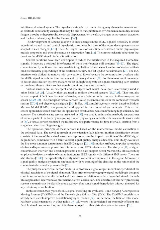
Sensors 2018, 18, 1388

intuitive and natural system. The myoelectric signals of a human being may change for reasons suchas electrode conductivity changes that may be due to transpiration or environmental humidity, musclefatigue, atrophy or hypertrophy, electrode displacement on the skin, changes in movement executionand the force intensity applied by the user [5–7].

The development of systems adaptive to these changes in the sEMG signal is necessary to obtainmore intuitive and natural control myoelectric prostheses, but most of the recent developments are notadapted to such changes [4–11]. The sEMG signal is a stochastic time-series based on the physiologicalmuscle properties and the subject muscle contraction form [12]. The same stochastic behaviour thatprovides the sEMG signal hinders its estimation.

Several solutions have been developed to reduce the interference in the acquired biomedicalsignals. However, a residual interference of these interferences still presents [13–20]. The signalcontamination by motion artifacts causes data irregularities. Nonetheless, the effects of motion artifactscan be reduced by proper design of the electronic circuitry and set-up, but not eliminated [21]. The ECGinterference is difficult to remove with conventional filters because the contamination overlaps withthe sEMG signal in both the time domain and frequency domain [22]. For these reasons, it is essentialto design classification systems that are robust enough to operate on signals containing such artifactsor can detect these artifacts so that signals containing them are discarded.

Virtual sensors are an emergent and intelligent tool which have been successfully used inother fields [23–26]. Usually, they are used to replace physical sensors [25,27,28]. They can alsobe used as part of fault detection methodologies, where their output is compared to the correspondingsensor [24,29–32]. The concept of virtual sensors is also present in studies in the context of wearablesensors [27,33] and physiological signals [34]. In Ref. [33], a multi-layer task model based on HiddenMarkov Model (HMM) was presented and applied in the context of gait analysis. This virtualsensor approach research confirms the application effectiveness while maintaining high efficiency andaccuracy. The virtual sensing service presented in [35] was used to estimate human body temperaturesof various parts of the body by integrating human physiological models with measurable sensor data.In [34], a virtual sensor estimated the respiratory rate performance for time intervals, starting from asingle-lead electrocardiogram signal.

The operation principle of these sensors is based on the mathematical model estimation ofthe collected data. The novel approach of the extensive fault-tolerant motion classification systemconsists of the use of the virtual sensor concept to reduce the impact over time of the sEMG signaldegradation, combined with a fault-tolerant signal quality analysis detector. This study evaluatedthe five most common contaminants in sEMG signals [7,11,36]: motion artifacts, amplifier saturation,electrode displacements, power line interference and ECG interference. The study in [11] of signalcontamination insertion and detection presents a one-class Support Vector Machine (SVM) successfullyemployed to detect a variety of contamination in sEMG signals with different SNR levels. There arealso studies [11,36] that specifically identify which contaminant is present in the signal. Moreover, asignal quality analysis system in conjunction with re-training of the classifier in the removal of thecontaminated channel is presented in [7].

The purpose of a virtual sensor model is to produce a signal output model independent of thephysical acquisition of the signal of interest. The surface electromyography signal modeling is designedcombining concepts of multichannel and their cross-correlation to replace degraded signal channels.This approach is referred to as multichannel cross-correlation. The objective of this new processingsystem is to maintain the classification accuracy after some signal degradation without the need forany retraining or calibration.

In this research, two types of sEMG signal modeling are evaluated: Time-Varying AutoregressiveMoving Average (TVARMA) and the Time-Varying Kalman filter (TVK). The TVARMA models havealready been used to improve non-stationary signal models [37]. Furthermore, the Kalman filter modelhas been used extensively in other fields [37–42], where it is considered an extremely efficient andflexible signal processing tool, and it is also employed in other virtual sensor enforcement [31].

77

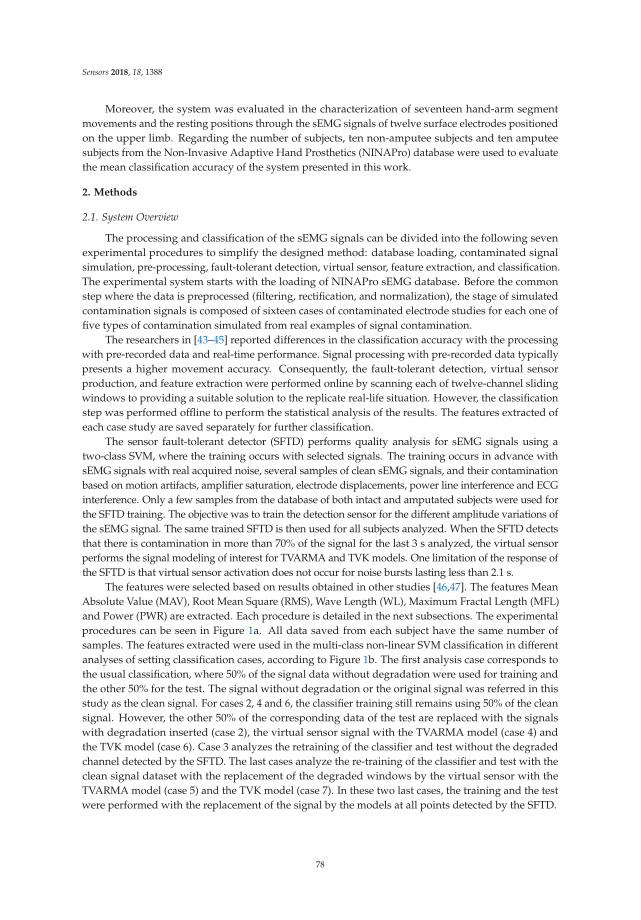
Sensors 2018, 18, 1388

Moreover, the system was evaluated in the characterization of seventeen hand-arm segmentmovements and the resting positions through the sEMG signals of twelve surface electrodes positionedon the upper limb. Regarding the number of subjects, ten non-amputee subjects and ten amputeesubjects from the Non-Invasive Adaptive Hand Prosthetics (NINAPro) database were used to evaluatethe mean classification accuracy of the system presented in this work.

2. Methods

2.1. System Overview

The processing and classification of the sEMG signals can be divided into the following sevenexperimental procedures to simplify the designed method: database loading, contaminated signalsimulation, pre-processing, fault-tolerant detection, virtual sensor, feature extraction, and classification.The experimental system starts with the loading of NINAPro sEMG database. Before the commonstep where the data is preprocessed (filtering, rectification, and normalization), the stage of simulatedcontamination signals is composed of sixteen cases of contaminated electrode studies for each one offive types of contamination simulated from real examples of signal contamination.

The researchers in [43–45] reported differences in the classification accuracy with the processingwith pre-recorded data and real-time performance. Signal processing with pre-recorded data typicallypresents a higher movement accuracy. Consequently, the fault-tolerant detection, virtual sensorproduction, and feature extraction were performed online by scanning each of twelve-channel slidingwindows to providing a suitable solution to the replicate real-life situation. However, the classificationstep was performed offline to perform the statistical analysis of the results. The features extracted ofeach case study are saved separately for further classification.

The sensor fault-tolerant detector (SFTD) performs quality analysis for sEMG signals using atwo-class SVM, where the training occurs with selected signals. The training occurs in advance withsEMG signals with real acquired noise, several samples of clean sEMG signals, and their contaminationbased on motion artifacts, amplifier saturation, electrode displacements, power line interference and ECGinterference. Only a few samples from the database of both intact and amputated subjects were used forthe SFTD training. The objective was to train the detection sensor for the different amplitude variations ofthe sEMG signal. The same trained SFTD is then used for all subjects analyzed. When the SFTD detectsthat there is contamination in more than 70% of the signal for the last 3 s analyzed, the virtual sensorperforms the signal modeling of interest for TVARMA and TVK models. One limitation of the response ofthe SFTD is that virtual sensor activation does not occur for noise bursts lasting less than 2.1 s.

The features were selected based on results obtained in other studies [46,47]. The features MeanAbsolute Value (MAV), Root Mean Square (RMS), Wave Length (WL), Maximum Fractal Length (MFL)and Power (PWR) are extracted. Each procedure is detailed in the next subsections. The experimentalprocedures can be seen in Figure 1a. All data saved from each subject have the same number ofsamples. The features extracted were used in the multi-class non-linear SVM classification in differentanalyses of setting classification cases, according to Figure 1b. The first analysis case corresponds tothe usual classification, where 50% of the signal data without degradation were used for training andthe other 50% for the test. The signal without degradation or the original signal was referred in thisstudy as the clean signal. For cases 2, 4 and 6, the classifier training still remains using 50% of the cleansignal. However, the other 50% of the corresponding data of the test are replaced with the signalswith degradation inserted (case 2), the virtual sensor signal with the TVARMA model (case 4) andthe TVK model (case 6). Case 3 analyzes the retraining of the classifier and test without the degradedchannel detected by the SFTD. The last cases analyze the re-training of the classifier and test with theclean signal dataset with the replacement of the degraded windows by the virtual sensor with theTVARMA model (case 5) and the TVK model (case 7). In these two last cases, the training and the testwere performed with the replacement of the signal by the models at all points detected by the SFTD.

78

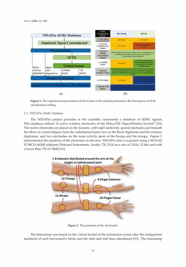
Sensors 2018, 18, 1388

(a) (b)

Figure 1. The experimental procedures (a) Flowchart of the method performed; (b) Description of SVMclassification setting.

2.2. NINAPro sEMG Database

The NINAPro project provides to the scientific community a database of sEMG signals.This database utilizes 12 active wireless electrodes of the DelsysTM TrignoWireless System® [48].The twelve electrodes are placed on the forearm, with eight uniformly spaced electrodes just beneaththe elbow at a fixed distance from the radiohumeral joint, two on the flexor digitorum and the extensordigitorum, and two electrodes on the main activity spots of the biceps and the triceps. Figure 2demonstrated the positions of the electrodes on the arm. NINAPro data is acquired using a NI-DAQPCMCIA 6024E platform (National Instruments, Austin, TX, USA) at a rate of 2 kHz, 12 bits and witha lower than 750 nV RMS [49].

Figure 2. The positions of the electrodes.

The timestamp was based on the virtual model of the orientation screen after the realignmenttreatment of each movement’s limits and the start and end time adjustment [50]. The timestamp

79

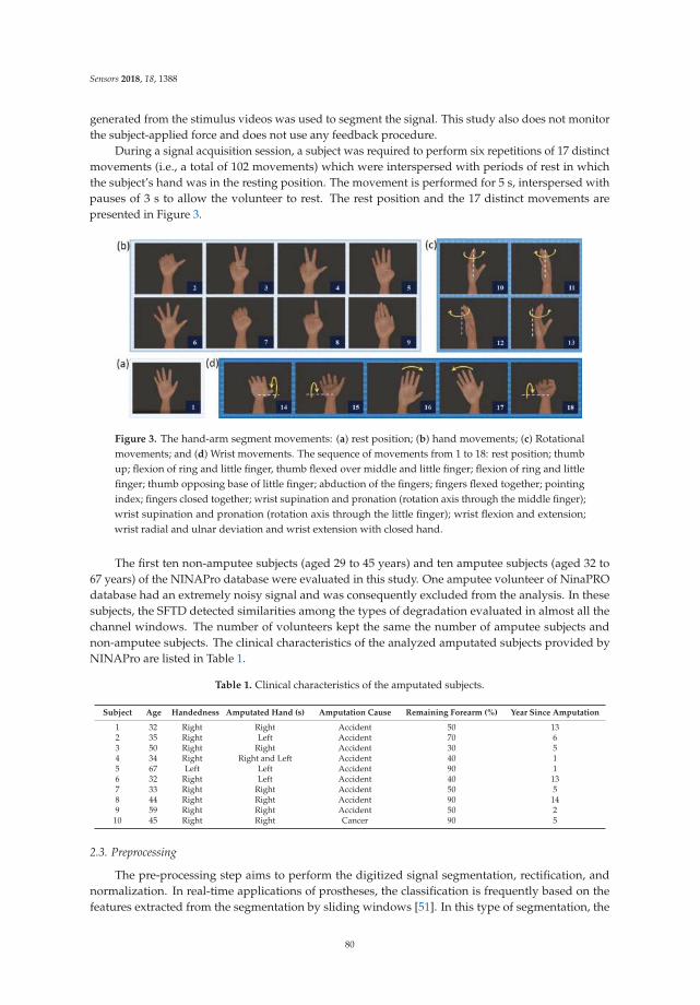
Sensors 2018, 18, 1388

generated from the stimulus videos was used to segment the signal. This study also does not monitorthe subject-applied force and does not use any feedback procedure.

During a signal acquisition session, a subject was required to perform six repetitions of 17 distinctmovements (i.e., a total of 102 movements) which were interspersed with periods of rest in whichthe subject’s hand was in the resting position. The movement is performed for 5 s, interspersed withpauses of 3 s to allow the volunteer to rest. The rest position and the 17 distinct movements arepresented in Figure 3.

Figure 3. The hand-arm segment movements: (a) rest position; (b) hand movements; (c) Rotationalmovements; and (d) Wrist movements. The sequence of movements from 1 to 18: rest position; thumbup; flexion of ring and little finger, thumb flexed over middle and little finger; flexion of ring and littlefinger; thumb opposing base of little finger; abduction of the fingers; fingers flexed together; pointingindex; fingers closed together; wrist supination and pronation (rotation axis through the middle finger);wrist supination and pronation (rotation axis through the little finger); wrist flexion and extension;wrist radial and ulnar deviation and wrist extension with closed hand.

The first ten non-amputee subjects (aged 29 to 45 years) and ten amputee subjects (aged 32 to67 years) of the NINAPro database were evaluated in this study. One amputee volunteer of NinaPROdatabase had an extremely noisy signal and was consequently excluded from the analysis. In thesesubjects, the SFTD detected similarities among the types of degradation evaluated in almost all thechannel windows. The number of volunteers kept the same the number of amputee subjects andnon-amputee subjects. The clinical characteristics of the analyzed amputated subjects provided byNINAPro are listed in Table 1.

Table 1. Clinical characteristics of the amputated subjects.

Subject Age Handedness Amputated Hand (s) Amputation Cause Remaining Forearm (%) Year Since Amputation

1 32 Right Right Accident 50 132 35 Right Left Accident 70 63 50 Right Right Accident 30 54 34 Right Right and Left Accident 40 15 67 Left Left Accident 90 16 32 Right Left Accident 40 137 33 Right Right Accident 50 58 44 Right Right Accident 90 149 59 Right Right Accident 50 2

10 45 Right Right Cancer 90 5

2.3. Preprocessing

The pre-processing step aims to perform the digitized signal segmentation, rectification, andnormalization. In real-time applications of prostheses, the classification is frequently based on thefeatures extracted from the segmentation by sliding windows [51]. In this type of segmentation, the

80

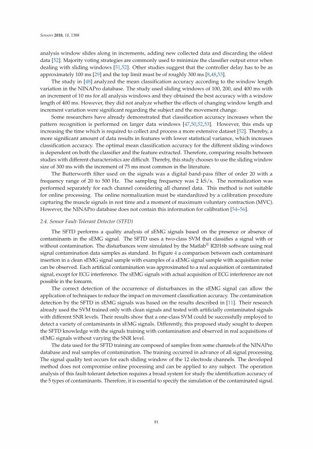
Sensors 2018, 18, 1388

analysis window slides along in increments, adding new collected data and discarding the oldestdata [52]. Majority voting strategies are commonly used to minimize the classifier output error whendealing with sliding windows [51,52]. Other studies suggest that the controller delay has to be asapproximately 100 ms [29] and the top limit must be of roughly 300 ms [8,48,53].

The study in [48] analyzed the mean classification accuracy according to the window lengthvariation in the NINAPro database. The study used sliding windows of 100, 200, and 400 ms withan increment of 10 ms for all analysis windows and they obtained the best accuracy with a windowlength of 400 ms. However, they did not analyze whether the effects of changing window length andincrement variation were significant regarding the subject and the movement change.

Some researchers have already demonstrated that classification accuracy increases when thepattern recognition is performed on larger data windows [47,50,52,53]. However, this ends upincreasing the time which is required to collect and process a more extensive dataset [52]. Thereby, amore significant amount of data results in features with lower statistical variance, which increasesclassification accuracy. The optimal mean classification accuracy for the different sliding windowsis dependent on both the classifier and the feature extracted. Therefore, comparing results betweenstudies with different characteristics are difficult. Thereby, this study chooses to use the sliding windowsize of 300 ms with the increment of 75 ms most common in the literature.

The Butterworth filter used on the signals was a digital band-pass filter of order 20 with afrequency range of 20 to 500 Hz. The sampling frequency was 2 kS/s. The normalization wasperformed separately for each channel considering all channel data. This method is not suitablefor online processing. The online normalization must be standardized by a calibration procedurecapturing the muscle signals in rest time and a moment of maximum voluntary contraction (MVC).However, the NINAPro database does not contain this information for calibration [54–56].

2.4. Sensor Fault-Tolerant Detector (STFD)

The SFTD performs a quality analysis of sEMG signals based on the presence or absence ofcontaminants in the sEMG signal. The SFTD uses a two-class SVM that classifies a signal with orwithout contamination. The disturbances were simulated by the Matlab® R2016b software using realsignal contamination data samples as standard. In Figure 4 a comparison between each contaminantinsertion in a clean sEMG signal sample with examples of a sEMG signal sample with acquisition noisecan be observed. Each artificial contamination was approximated to a real acquisition of contaminatedsignal, except for ECG interference. The sEMG signals with actual acquisition of ECG interference are notpossible in the forearm.

The correct detection of the occurrence of disturbances in the sEMG signal can allow theapplication of techniques to reduce the impact on movement classification accuracy. The contaminationdetection by the SFTD in sEMG signals was based on the results described in [11]. Their researchalready used the SVM trained only with clean signals and tested with artificially contaminated signalswith different SNR levels. Their results show that a one-class SVM could be successfully employed todetect a variety of contaminants in sEMG signals. Differently, this proposed study sought to deepenthe SFTD knowledge with the signals training with contamination and observed in real acquisitions ofsEMG signals without varying the SNR level.

The data used for the SFTD training are composed of samples from some channels of the NINAProdatabase and real samples of contamination. The training occurred in advance of all signal processing.The signal quality test occurs for each sliding window of the 12 electrode channels. The developedmethod does not compromise online processing and can be applied to any subject. The operationanalysis of this fault-tolerant detection requires a broad system for study the identification accuracy ofthe 5 types of contaminants. Therefore, it is essential to specify the simulation of the contaminated signal.

81

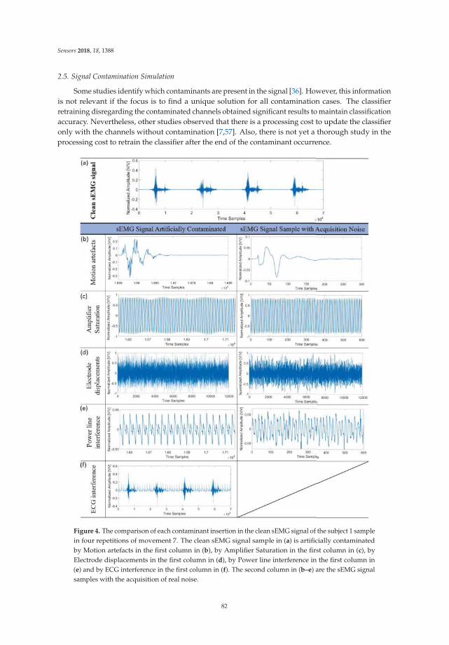
Sensors 2018, 18, 1388

2.5. Signal Contamination Simulation

Some studies identify which contaminants are present in the signal [36]. However, this informationis not relevant if the focus is to find a unique solution for all contamination cases. The classifierretraining disregarding the contaminated channels obtained significant results to maintain classificationaccuracy. Nevertheless, other studies observed that there is a processing cost to update the classifieronly with the channels without contamination [7,57]. Also, there is not yet a thorough study in theprocessing cost to retrain the classifier after the end of the contaminant occurrence.

Figure 4. The comparison of each contaminant insertion in the clean sEMG signal of the subject 1 samplein four repetitions of movement 7. The clean sEMG signal sample in (a) is artificially contaminatedby Motion artefacts in the first column in (b), by Amplifier Saturation in the first column in (c), byElectrode displacements in the first column in (d), by Power line interference in the first column in(e) and by ECG interference in the first column in (f). The second column in (b–e) are the sEMG signalsamples with the acquisition of real noise.

82

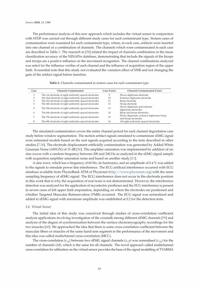
Sensors 2018, 18, 1388

The performance analysis of this new approach which includes the virtual sensor in conjunctionwith STDF was carried out through different study cases for each contaminant type. Sixteen cases ofcontamination were examined for each contaminant type, where, in each case, artifacts were insertedinto one channel or a combination of channels. The channels which were contaminated in each caseare described in Table 2. The research in [58] related the impact of channels combination in the meanclassification accuracy of the NINAPro database, demonstrating that include the signals of the bicepsand triceps are a positive influence on the movement recognition. The channel combinations analyzedwas select for the influence verifies of each channel and the influence of acquisition region of the upperlimb. It essential note that this study not evaluated the variation effect of SNR and not changing thegain of the artifact signal before insertion.

Table 2. Channels contaminated in sixteen cases for each contaminant type.

Case Channels Contaminated Case (Cont.) Channels Contaminated (Cont.)

1 The 1st electrode of eight uniformly spaced electrodes 9 Flexor digitorum electrode2 The 2nd electrode of eight uniformly spaced electrodes 10 Extensor digitorum electrode3 The 3rd electrode of eight uniformly spaced electrodes 11 Bicep electrode4 The 4th electrode of eight uniformly spaced electrodes 12 Tricep electrode

5 The 5th electrode of eight uniformly spaced electrodes 13Flexor digitorum and extensordigitorum electrodes

6 The 6th electrode of eight uniformly spaced electrodes 14 Bicep and tricep electrodes

7 The 7th electrode of eight uniformly spaced electrodes 15Flexor digitorum, extensor digitorum, bicepand tricep electrodes

8 The 8th electrode of eight uniformly spaced electrodes 16 All eight uniformly spaced electrodes

The simulated contamination covers the entire channel period for each channel degradation casestudy before window segmentation. The motion artifact signals simulated to contaminate sEMG signalwere estimated models based on the real signals acquired according to the tests described in otherstudies [7,36]. The electrode displacement artificially contamination was generated by Added WhiteGaussian Noise (AWGN) of 15 dB [36]. The amplifier saturation was implemented by addition of sixsine waves with a random frequency between 200 and 240 Hz as analyzed in the sEMG signal samplewith acquisition amplifier saturation noise and based on another study [11].

A sine wave, which has a frequency of 60 Hz, its harmonics, and an amplitude of 0.4 V, was addedto the signals to simulate power line interference. The ECG artificial interference occurred with ECGdatabase available from PhysioBank ATM of Physionet (http://www.physionet.org) with the samesampling frequency of sEMG signal. The ECG interference does not occur in the electrode positionin this work that is why the acquisition of real noise is not demonstrated. However, the interferencedetection was analyzed for the application of myoelectric protheses and the ECG interference is presentin severe cases of left upper limb amputation, depending on where the electrodes are positioned andwhether Targeted Muscular Reinnervation (TMR) occurred. The ECG signal was normalized andadded to sEMG signal with maximum amplitude was established at 0.2 for the detection tests.

2.6. Virtual Sensor

The initial idea of this study was conceived through studies of cross-correlation coefficientanalysis applications involving investigation of the crosstalk among different sEMG channels [59] andanalysis of the degree of synchronization between the surface electromyography recordings for thetwo muscles [60]. We approached the idea that there is some cross-correlation coefficient between themuscular fibers or muscles of the same hand-arm segment in the performance of the movement andthis idea was called multichannel cross-correlation (MCC).

The cross-correlation (rxy) between two sEMG signal channels (x, y) was normalised (cxy) for thenumber of channels (M), which is the same for all channels. The novel approach called multichannelcross-correlation for utilization on the virtual sensor provides the base of the signal modelling of TVARMA

83

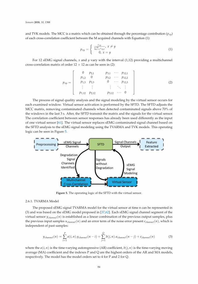
Sensors 2018, 18, 1388

and TVK models. The MCC is a matrix which can be obtained through the percentage contribution (pxy)of each cross-correlation coefficient between the M acquired channels with Equation (1):

pxy =

{ cxy

∑Mi=1 cxy,i

, x �= y

0, x = y(1)

For 12 sEMG signal channels, x and y vary with the interval (1,12) providing a multichannelcross-correlation matrix of order 12 × 12 as can be seen in (2):

pxy =

⎡⎢⎢⎢⎢⎢⎢⎣

0 p2,1

p1,2 0p1,3 p2,3...

...p1,12 p2,12

p3,1 · · · p12,1

p3,2 · · · p12,2

0 · · · p12,3...

. . ....

p3,12 · · · 0

⎤⎥⎥⎥⎥⎥⎥⎦

(2)

The process of signal quality analysis and the signal modeling by the virtual sensor occurs foreach examined window. Virtual sensor activation is performed by the SFTD. The SFTD adjusts theMCC matrix, removing contaminated channels when detected contaminated signals above 70% ofthe windows in the last 3 s. After, the SFTD transmit the matrix and the signals for the virtual sensor.The correlation coefficient between sensor responses has already been used differently as the inputof one virtual sensor [61]. The virtual sensor replaces sEMG contaminated signal channel based onthe SFTD analysis to the sEMG signal modeling using the TVARMA and TVK models. This operatinglogic can be seen in Figure 5.

Figure 5. The operating logic of the SFTD with the virtual sensor.

2.6.1. TVARMA Model

The proposed sEMG signal TVARMA model for the virtual sensor at time n can be represented in(3) and was based on the sEMG model proposed in [37,62]. Each sEMG signal channel segment of thevirtual sensor ychannel(n) is established as a linear combination of the previous output samples, plusthe previous input samples uchannel(n) and an error term of the noise error present echannel(n), which isindependent of past samples:

ychannel(n) =P

∑i=1

a(i, n).ychannel(n − i) +Q

∑j=1

b(j, n).uchannel(n − j) + echannel(n) (3)

where the a(i, n) is the time-varying autoregressive (AR) coefficient, b(j, n) is the time-varying movingaverage (MA) coefficient and the indexes P and Q are the highest orders of the AR and MA models,respectively. The model has the model orders set to 4 for P and 2 for Q.

84

Sensors 2018, 18, 1388

The input samples uchannel(n − j) can be obtained through Equation (4), which uses the respectivechannel of interest’s column of the MCC matrix and the other channel samples considered as cleansignals from sEMG

→y (n − i). The channels with known contamination have the correlation coefficient

line set to zero:

uchannel(n − j) =(→

p x,channel

)T.→y (n − i) (4)

where→p x,channel is the respective values column of the percentage contribution of the cross-correlation

coefficient between the channel of interest and the other channels.A finite-order base function f (n, m) was imposed for the functions of parameters a(i, n) and b(j, n)

to obtain a better model in Equations (5) and (6). These functions were proposed in other studies ofTVARMA models [62,63]:

a(i, n) =V

∑m=0

α(i, m) f (n, m) (5)

b(j, n) =V

∑m=0

β(j, m) f (n, m) (6)

where f (n, m) with m = 0, 1, 2, . . . , V and n = 0, 1, 2, . . . , N − 1 is the base function that needs tobe selected. The parameter functions α(i, m) and β(j, m) represent the expansion of the parameterswith V, which is the maximum number of base sequences [62]. Therefore, the proposed sEMG signalsTVARMA model is finally defined as shown in (7):

ychannel(n) =P

∑i=1

V

∑m=0

α(i, m).ychannel(n − i) +Q

∑j=1

V

∑m=0

β(j, m).uchannel(n − j) + echannel(n) (7)

2.6.2. TVK Model

The TVK model of sEMG signals for the virtual sensor is based on Kalman state estimator that isgiven a state-space model with satisfactory known inputs uchannel(n), white process noise w(n), andwhite measurement noise v(n). The virtual sensor measurement ychannel(n) and the state equationx(n) can be represented by Equation (8):

x(n + 1) = Ax(n) + Buchannel(n) + Gw(n)

ychannel(n) = Cx(n) + v(n)(8)

where A, B, C, and G are state matrices.The ychannel(n) and uchannel(n) are estimated in the same way as reported for the TVARMA

models. The estimator generates output estimates y[n|n] and state estimates x[n|n] using all availablemeasurements up to ychannel(n). The state estimator can be represented as in (9):

x[n + 1|n] = Ax[n|(n − 1)] + Buchannel(n) + M(ychannel(n)− Cx[n|(n − 1)]) (9)

where M is the innovation gain, which updates the prediction x[n + 1|n] using the new measurementychannel(n), and it is determined by solving an algebraic Riccati equation in (10), where P solves thecorresponding equation:

M = PCT(

CPCT + R)−1

(10)

The final estimator y[n|n] for the virtual sensor has the following output equation:

[y[n|n]x[n|n]

]=

[C(I − MC)

I − MC

]x[n|n − 1] +

[CM

M

]ychannel [n|n] (11)

85

Sensors 2018, 18, 1388

The matrices of the TVK model were set with the identity matrix. The sEMG signals models wereapplied to all sliding windows detected by the SFTD for each subject in the sixteen different casesreported for each simulated signal contamination.

2.7. Feature Extraction

The efficiency of the sEMG signal classification system depends on the choice of features [64].However, the features selected may be redundant or even irrelevant [65]. Each feature is not equallynecessary for a specific task. The features were selected based on the result of the classification of otherstudies [46,53,66] with the same database and the evaluation of characteristics for sEMG [47].

The characteristics were extracted from each sliding window and the features selection in thetime domain is directly related to the MMC concept, which analyses the percentage contribution ofeach cross-correlation coefficient of two sEMG signal channels in the time domain. It is important toemphasize that no feature reduction technique was used. The combination of the MAV, RMS, WL,MFL, and PWR features presented better mean classification accuracy results for the analyzed subjects.

2.8. Classification with Support Vector Machines

The non-linear SVM classification with radial basis function (RBF) kernel was implemented inthe sEMG signals classification of all simulated cases. The kernel functions parameters were selectedby a search algorithm of the best result for each subject. The multi-class definition technique forclassifying movement was eighteen binary classifications of one versus all. In more than one positiveclass case, the algorithm selects the class that is farthest away from the hyperplane that separates eachbinary classification.

The majority voting technique is used as a post-processing mechanism considering last threewindow classification. Also, the k-fold complimentary technique was applied for improving thereliable accuracy test with the small number of samples in which the model is trained and tested.The tests are carried out in all possible different input conditions forming 20 k-folds for the six availablemovement repetitions. For each k-fold, three of the six repetitions (50% of the dataset) were selectedfor the training model and three (50% of the dataset) for testing.

The classification procedure was applied to seven different settings, according to the Figure 1b.The classification using the signal without contamination performed the usual training and test in theaverage of all possible k-folds. The classification analyses of the signal contamination were performedby training the classifier with the data part of the signal without degradation and the test with the othercorresponding part in each separate case for the signal with degradation inserted. The classificationsusing the virtual sensor occur similar to the previous, the data part of the signal without degradationwas used for training, but the signals with TVARMA model and TVK model replace the degradationinserted detected for STFD for the test.

The seven different settings include the re-training practice of the classifier for comparativeperformance analysis. The classification re-training without the degraded channel was performed when80% of the windows were considered contaminated by the SFTD. The classification with re-trainingusing the two signals modeled was made through the contaminated signal replacement by the virtualsensor in the training and testing. For every sliding window that featured 70% of contaminationdetected by the SFTD in the last 3 s, the virtual sensor replaced the sEMG signal by the modeled signal.This threshold was established based on another study [57], which introduced the idea of contaminanttemporality and the return to reconsideration of the contaminated channel. Each subject was analyzedfor different contamination types in different channel arrangements, and each analysis resulted in aspecific confusion matrix of all k-folds each classification results.

2.9. Experimental Statistical Analysis

Design and analysis of three-factor experiments were entirely randomized and used for thestatistical validation of the test methodology. A Design of Experiments full factorial design [67] was

86

Sensors 2018, 18, 1388

realized with the mean accuracy response variable and the controllable factors: the classification settingtype, the contaminant signal inserted and the variation cases of channel contaminations. The modelused follows in (12):

y_ijk = μ + α_i + β_j + γ_k + (αβ)_ij + (αγ)_ik + (βγ)_jk + (αβγ)_ijk + ε_ijk (12)

where y_ijk corresponds to the level i response in repetition j, μ corresponds to the general average,α_i corresponds to the effect of each level i and ε_ijk corresponds to the error of level i in repetition j.

Analyses of variance (ANOVA) and multiple comparisons also were used for providing astatistical test, which makes possible to assert whether the various group’s average differencesare significant or not. Two averages are significantly different when their intervals are disjointed.When their intervals overlap, they are not significantly different.

3. Results

The signal processing was analyzed for ten intact subjects and ten amputees. It is importantto note that the proposed method using a virtual sensor is independent of the pattern algorithmbecause the virtual sensor is applied before classification. The SFTD detection and the movementclassification used the algorithm SVM. However, there is no dependency on this algorithm. This newextensive fault-tolerant system could use any other algorithm. The SVM is widely used in sEMGsignals [46,68–72] and was selected to compare and evaluate the effectiveness of this new system.

3.1. SFTD Results

For the correct interpretation of the results, an analysis of the detection of the windowscontaminated by the SFTD is necessary. The SFTD detection accuracy of 85.31 ± 24.88%and false-positive recognition for the channels that non-received the artificial contamination of8.18 ± 17.52% demonstrated the sensibility of sensor detection. All acquired signal has noise, evenafter preprocessing, since there may be noises in the frequency range of the sEMG signals.

The SFTD has a differentiation in detection depending on the analyzed contaminant. The ECGand power line interference detection have obtained lower precisions. These contaminants present aneffect of lower significance than the other three disturbances. The detection of the ECG and power lineinterferences in channel 12, which corresponds to the electrode positioned on the triceps, obtained aprecision lower than 20% of the average of the other channels. The acquired channel 12 also featuresthe low representativity of the sEMG signal compared to the noise level of the channel. This lowrepresentativity may explain the accuracy detection decrease of the SFTD since channel 12 does notseem to be significantly relevant to the movement classification.

3.2. Movement Classification Results

Figure 6 presents the mean classification accuracy for all 16 noise insertion cases with differentchannel combinations.

In Figure 6, it is possible to realize that each contamination type impairs the classificationdifferently in comparison to the clean signal classification (legend 1), in which some contaminations aremore expressively than others, such as saturation and displacement of electrodes. For contaminationby electrode displacement and saturation, the substitution of the contaminated signal by the signalsmodeled with TVARMA (legend 4) and TVK (legend 6) recovers at least 30% of the mean accuracyclassification. For contamination by movement artifacts, recovery is at least 20% for intact subjects andapproximately 4% for amputated subjects. For ECG contamination and power line interference, thecontaminated signal replaced by the virtual sensor models only further damages the signal.

In the comparison of the classifier retraining with removal of the contaminated channel (legend 3),the classifier retraining with the contaminated channel entirely replaced by the virtual sensor usingthe TVARMA model (legend 5) and using the TVK model (legend 6) demonstrate the improvement

87

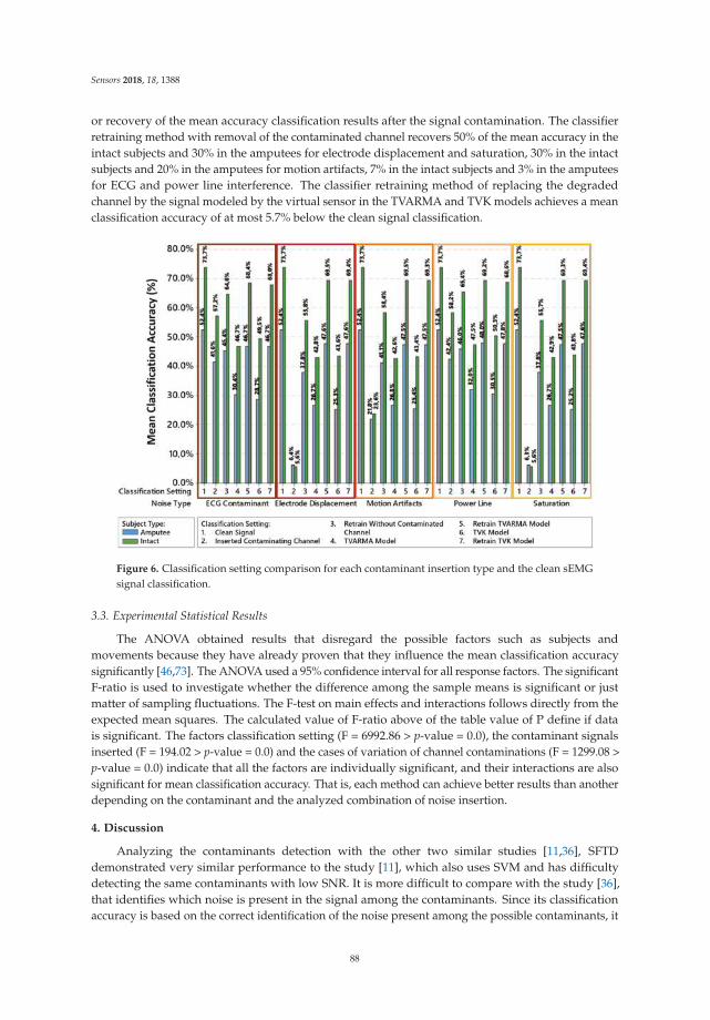
Sensors 2018, 18, 1388

or recovery of the mean accuracy classification results after the signal contamination. The classifierretraining method with removal of the contaminated channel recovers 50% of the mean accuracy in theintact subjects and 30% in the amputees for electrode displacement and saturation, 30% in the intactsubjects and 20% in the amputees for motion artifacts, 7% in the intact subjects and 3% in the amputeesfor ECG and power line interference. The classifier retraining method of replacing the degradedchannel by the signal modeled by the virtual sensor in the TVARMA and TVK models achieves a meanclassification accuracy of at most 5.7% below the clean signal classification.

Figure 6. Classification setting comparison for each contaminant insertion type and the clean sEMGsignal classification.

3.3. Experimental Statistical Results

The ANOVA obtained results that disregard the possible factors such as subjects andmovements because they have already proven that they influence the mean classification accuracysignificantly [46,73]. The ANOVA used a 95% confidence interval for all response factors. The significantF-ratio is used to investigate whether the difference among the sample means is significant or justmatter of sampling fluctuations. The F-test on main effects and interactions follows directly from theexpected mean squares. The calculated value of F-ratio above of the table value of P define if datais significant. The factors classification setting (F = 6992.86 > p-value = 0.0), the contaminant signalsinserted (F = 194.02 > p-value = 0.0) and the cases of variation of channel contaminations (F = 1299.08 >p-value = 0.0) indicate that all the factors are individually significant, and their interactions are alsosignificant for mean classification accuracy. That is, each method can achieve better results than anotherdepending on the contaminant and the analyzed combination of noise insertion.

4. Discussion

Analyzing the contaminants detection with the other two similar studies [11,36], SFTDdemonstrated very similar performance to the study [11], which also uses SVM and has difficultydetecting the same contaminants with low SNR. It is more difficult to compare with the study [36],that identifies which noise is present in the signal among the contaminants. Since its classificationaccuracy is based on the correct identification of the noise present among the possible contaminants, it

88

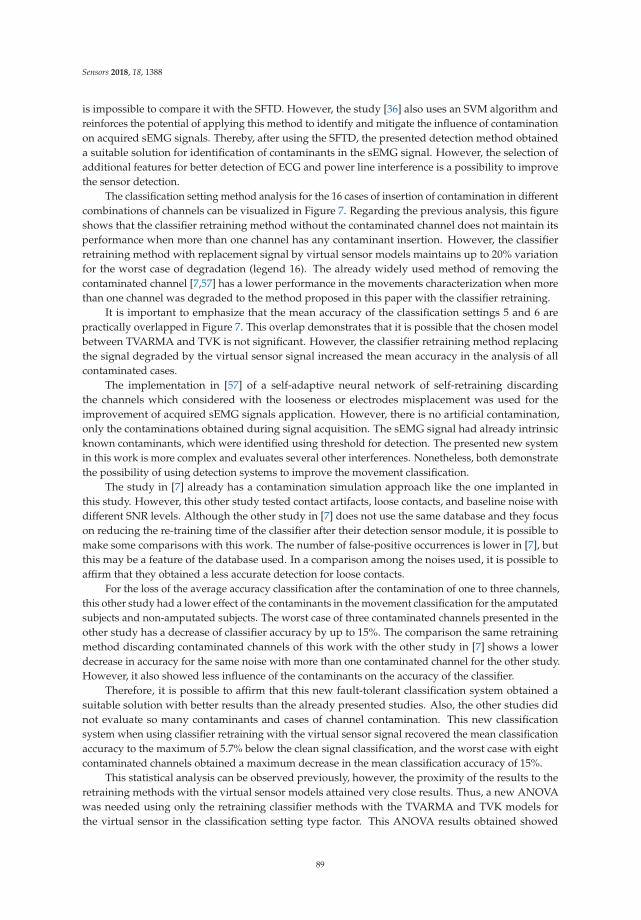
Sensors 2018, 18, 1388

is impossible to compare it with the SFTD. However, the study [36] also uses an SVM algorithm andreinforces the potential of applying this method to identify and mitigate the influence of contaminationon acquired sEMG signals. Thereby, after using the SFTD, the presented detection method obtaineda suitable solution for identification of contaminants in the sEMG signal. However, the selection ofadditional features for better detection of ECG and power line interference is a possibility to improvethe sensor detection.

The classification setting method analysis for the 16 cases of insertion of contamination in differentcombinations of channels can be visualized in Figure 7. Regarding the previous analysis, this figureshows that the classifier retraining method without the contaminated channel does not maintain itsperformance when more than one channel has any contaminant insertion. However, the classifierretraining method with replacement signal by virtual sensor models maintains up to 20% variationfor the worst case of degradation (legend 16). The already widely used method of removing thecontaminated channel [7,57] has a lower performance in the movements characterization when morethan one channel was degraded to the method proposed in this paper with the classifier retraining.

It is important to emphasize that the mean accuracy of the classification settings 5 and 6 arepractically overlapped in Figure 7. This overlap demonstrates that it is possible that the chosen modelbetween TVARMA and TVK is not significant. However, the classifier retraining method replacingthe signal degraded by the virtual sensor signal increased the mean accuracy in the analysis of allcontaminated cases.

The implementation in [57] of a self-adaptive neural network of self-retraining discardingthe channels which considered with the looseness or electrodes misplacement was used for theimprovement of acquired sEMG signals application. However, there is no artificial contamination,only the contaminations obtained during signal acquisition. The sEMG signal had already intrinsicknown contaminants, which were identified using threshold for detection. The presented new systemin this work is more complex and evaluates several other interferences. Nonetheless, both demonstratethe possibility of using detection systems to improve the movement classification.

The study in [7] already has a contamination simulation approach like the one implanted inthis study. However, this other study tested contact artifacts, loose contacts, and baseline noise withdifferent SNR levels. Although the other study in [7] does not use the same database and they focuson reducing the re-training time of the classifier after their detection sensor module, it is possible tomake some comparisons with this work. The number of false-positive occurrences is lower in [7], butthis may be a feature of the database used. In a comparison among the noises used, it is possible toaffirm that they obtained a less accurate detection for loose contacts.

For the loss of the average accuracy classification after the contamination of one to three channels,this other study had a lower effect of the contaminants in the movement classification for the amputatedsubjects and non-amputated subjects. The worst case of three contaminated channels presented in theother study has a decrease of classifier accuracy by up to 15%. The comparison the same retrainingmethod discarding contaminated channels of this work with the other study in [7] shows a lowerdecrease in accuracy for the same noise with more than one contaminated channel for the other study.However, it also showed less influence of the contaminants on the accuracy of the classifier.

Therefore, it is possible to affirm that this new fault-tolerant classification system obtained asuitable solution with better results than the already presented studies. Also, the other studies didnot evaluate so many contaminants and cases of channel contamination. This new classificationsystem when using classifier retraining with the virtual sensor signal recovered the mean classificationaccuracy to the maximum of 5.7% below the clean signal classification, and the worst case with eightcontaminated channels obtained a maximum decrease in the mean classification accuracy of 15%.

This statistical analysis can be observed previously, however, the proximity of the results to theretraining methods with the virtual sensor models attained very close results. Thus, a new ANOVAwas needed using only the retraining classifier methods with the TVARMA and TVK models forthe virtual sensor in the classification setting type factor. This ANOVA results obtained showed

89

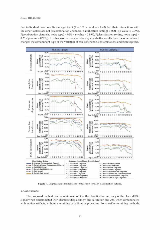
Sensors 2018, 18, 1388

that individual mean results are significant (F = 0.62 > p-value = 0.43), but their interactions withthe other factors are not (F(combination channels, classification setting) = 0.21 < p-value = 0.999),F(combination channels, noise type) = 0.51 < p-value = 0.999), F(classification setting, noise type) =0.25 < p-value = 0.908)). In other words, one model always has better results than the other when itchanges the contaminant type or the variation of cases of channel contaminations and both together.

Figure 7. Degradation channel cases comparison for each classification setting.

5. Conclusions

The proposed method can maintain over 60% of the classification accuracy of the clean sEMGsignal when contaminated with electrode displacement and saturation and 20% when contaminatedwith motion artifacts, without a retraining or calibration procedure. For classifier retraining methods,

90

Sensors 2018, 18, 1388

the replacement of the contaminated channel by the virtual sensor model demonstrates the best resultsfor all types of contaminants.

The statistical experimental results determined that the variation of the classification setting,the contaminant signal inserted and the cases channel contaminations significantly affect the meanclassification accuracy. The comparison and statistical analysis of the virtual sensor method with theTVARMA and TVK models demonstrate that the TVARMA model obtains more significant meanaccuracy for the variation of the contaminant signal inserted, for the variation of cases channelcontaminations and both together.

The SFTD accuracy was obtained using a training base of intact subjects and amputees. It is maybe possible to improve this accuracy by dividing the intact subjects and amputees for training SFTD.However, it is necessary the controlled acquisition of contaminants in amputees, and calibration maybe required, because of the uniqueness of each amputee’s muscular integrity.

The quality analysis and virtual sensor model run online at the same time for both TVARMAand TVK models. The processing time of the virtual sensors with the SFTD was not computed.The classification is performed offline later to generate the results of the statistical tests. The algorithmof the proposed system can be optimized for the user online application in the next steps, consideringthe results analyzed in this work. Classification accuracy cannot be determined in most surveys sincedifferent movements and subjects are evaluated. The use of a public database such as NINAPro enablesthe scientific community to evaluate the contribution of this innovation. It is important to note thatproposed technic of adaptation can be a form of complementation with several other approaches suchas user adaptation with online feedback [74].

The proposed system is a complementary technique to increase the clinical impact of themyoelectric prosthesis or other applications with the same stochastic behavior signals. For example,EEG for seizure detection, ECG for QRS detection or arrhythmia classification. However, the next stepin this research will be the improvement of virtual sensor model adaptation for frequency featuresand consequently the classification results enhancement. In parallel, an adjustment of SFTD methodshould be developed for ECG and power line interference.

Author Contributions: Karina de O. A. de Moura conceived the methodology, as well as designed and performedthe experiments, processed and analyzed the data, performed the statistical analysis. Alexandre Balbinotcontributed to the concept and ideas, implementation of the proposed and checked the system methodology.All authors participated in the result analysis, and the paper revision.

Funding: This research supported by National Counsel of Technological and Scientific Development (CNPq).

Acknowledgments: This research was performed at the Electro-Electronic Instrumentation (IEE) laboratoryof the Federal University of Rio Grande do Sul. The authors would like to thank all the collaboration oflaboratory colleagues.

Conflicts of Interest: The authors declare no conflict of interest.

References

1. Deijs, M.; Bongers, R.M.; Ringeling-van Leusen, N.D.M.; van der Sluis, C.K. Flexible and static wristunits in upper limb prosthesis users: Functionality scores, user satisfaction and compensatory movements.J. Neuroeng. Rehabilt. 2016, 13, 26. [CrossRef] [PubMed]

2. Engdahl, S.M.; Christie, B.P.; Kelly, B.; Davis, A.; Chestek, C.A.; Gates, D.H. Surveying the interest ofindividuals with upper limb loss in novel prosthetic control techniques. J. Neuroeng. Rehabilt. 2015, 12, 53.[CrossRef] [PubMed]

3. Zhang, D.; Zhao, X.; Han, J.; Zhao, Y. A comparative study on PCA and LDA based EMG pattern recognitionfor anthropomorphic robotic hand. In Proceedings of the 2014 IEEE International Conference on Roboticsand Automation (ICRA), Hong Kong, China, 31 May–7 June 2014; pp. 4850–4855. [CrossRef]

4. Blana, D.; Kyriacou, T.; Lambrecht, J.M.; Chadwick, E.K. Feasibility of using combined EMG and kinematicsignals for prosthesis control: A simulation study using a virtual reality environment. J. Electromyogr. Kinesiol.

2016, 29, 21–27. [CrossRef] [PubMed]

91

Sensors 2018, 18, 1388

5. Sensinger, J.W.; Lock, B.A.; Kuiken, T.A. Adaptive pattern recognition of myoelectric signals: Exploration ofconceptual framework and practical algorithms. IEEE Trans. Neural Syst. Rehabilt. Eng. 2009, 17, 270–278.[CrossRef] [PubMed]

6. Liu, J. Adaptive myoelectric pattern recognition toward improved multifunctional prosthesis control.Med. Eng. Phys. 2015, 37, 424–430. [CrossRef] [PubMed]

7. Zhang, X.; Huang, H. A real-time, practical sensor fault-tolerant module for robust EMG pattern recognition.J. Neuroeng. Rehabilt. 2015, 12, 18. [CrossRef] [PubMed]

8. Jiang, N.; Lorrain, T.; Farina, D. A state-based, proportional myoelectric control method: Online validationand comparison with the clinical state-of-the-art. J. Neuroeng. Rehabilt. 2014, 11, 110. [CrossRef] [PubMed]

9. Atzori, M.; Müller, H. Control Capabilities of Myoelectric Robotic Prostheses by Hand Amputees: A ScientificResearch and Market Overview. Front. Syst. Neurosci. 2015, 9, 162. [CrossRef] [PubMed]

10. Spanias, J.; Perreault, E.; Hargrove, L. Detection of and Compensation for EMG Disturbances for PoweredLower Limb Prosthesis Control. IEEE Trans. Neural Syst. Rehabilt. Eng. 2015, 4320, 226–234. [CrossRef][PubMed]

11. Fraser, G.D.; Chan, A.D.C.; Green, J.R.; MacIsaac, D.T. Automated Biosignal Quality Analysis forElectromyography Using a One-Class Support Vector Machine. IEEE Trans. Instrum. Meas. 2014, 63, 2919–2930.[CrossRef]

12. Zivanovic, M. Time-Varying Multicomponent Signal Modeling for Analysis of Surface EMG Data. IEEE Signal

Process. Lett. 2014, 21, 692–696. [CrossRef]13. Tomasini, M.; Benatti, S.; Milosevic, B.; Farella, E.; Benini, L. Power Line Interference Removal for

High-Quality Continuous Biosignal Monitoring with Low-Power Wearable Devices. IEEE Sens. J. 2016,16, 3887–3895. [CrossRef]

14. Mastinu, E.; Ahlberg, J.; Lendaro, E.; Hermansson, L.; Hakansson, B.; Ortiz-Catalan, M. An alternativemyoelectric pattern recognition approach for the control of hand prostheses: A case study of use in daily lifeby a dysmelia subject. IEEE J. Transl. Eng. Health Med. 2018, 6. [CrossRef] [PubMed]

15. Zhang, X.; Huang, H.; Yang, Q. Real-time implementation of a self-recovery EMG pattern recognitioninterface for artificial arms. In Proceedings of the 2013 35th Annual International Conference of the IEEEEngineering in Medicine and Biology Society (EMBC), Osaka, Japan, 3–7 July 2013; pp. 5926–5929. [CrossRef]

16. Favieiro, G.; Cene, V.H.; Balbinot, A. Self-adaptive method for sEMG movement classification based oncontinuous optimal electrode assortment. Braz. J. Instrum. Control 2016, 4, 21–26. [CrossRef]

17. Chowdhury, R.H.; Reaz, M.B.; Ali, M.A.B.M.; Bakar, A.A.; Chellappan, K.; Chang, T.G.Surface Electromyography Signal Processing and Classification Techniques. Sensors 2013, 13, 12431–12466.[CrossRef] [PubMed]

18. Soedirdjo, S.D.H.; Ullah, K.; Merletti, R. Power line interference attenuation in multi-channel sEMG signals:Algorithms and analysis. In Proceedings of the 2015 37th Annual International Conference of the IEEEEngineering in Medicine and Biology Society (EMBC), Milan, Italy, 25–29 Augst 2015; pp. 3823–3826.[CrossRef]

19. Fraser, G.D.; Chan, A.D.C.; Green, J.R.; Abser, N.; MacIsaac, D. CleanEMG—Power line interferenceestimation in sEMG using an adaptive least squares algorithm. In Proceedings of the 2011 AnnualInternational Conference of the IEEE Engineering in Medicine and Biology Society, Boston, MA, USA,30 August–3 September 2011; pp. 7941–7944. [CrossRef]

20. Zhang, Y.; Su, S.; Xu, P.; Yao, D. Performance evaluation of Noise-Assisted Multivariate Empirical ModeDecomposition and its application to multichannel EMG signals. In Proceedings of the 2017 39th AnnualInternational Conference of the IEEE Engineering in Medicine and Biology Society (EMBC), Seogwipo,Korea, 11–15 July 2017; pp. 3457–3460. [CrossRef]

21. Nazmi, N.; Abdul Rahman, M.; Yamamoto, S.; Ahmad, S.; Zamzuri, H.; Mazlan, S. A Review of ClassificationTechniques of EMG Signals during Isotonic and Isometric Contractions. Sensors 2016, 16, 1304. [CrossRef][PubMed]

22. Chen, M.; Zhang, X.; Chen, X.; Zhu, M.; Li, G.; Zhou, P. FastICA peel-off for ECG interference removal fromsurface EMG. Biomed. Eng. Online 2016, 15, 65. [CrossRef] [PubMed]

23. Sánchez-Molina, J.A.; Rodríguez, F.; Guzmán, J.L.; Ramírez-arias, J.A. Water content virtual sensor fortomatoes in coconut coir substrate for irrigation control design. Agric. Water Manag. 2015, 151, 114–125.[CrossRef]

92

Sensors 2018, 18, 1388

24. Ponsart, J.C.; Theilliol, D.; Aubrun, C. Virtual sensors design for active fault tolerant control system appliedto a winding machine. Control Eng. Pract. 2010, 18, 1037–1044. [CrossRef]

25. Ploennigs, J.; Ahmed, A.; Hensel, B.; Stack, P.; Menzel, K. Virtual sensors for estimation of energy consumptionand thermal comfort in buildings with underfloor heating. Adv. Eng. Inform. 2011, 25, 688–698. [CrossRef]

26. Fagiano, L.; Novara, C. A combined Moving Horizon and Direct Virtual Sensor approach for constrainednonlinear estimation. Automatica 2013, 49, 193–199. [CrossRef]

27. Liu, K.; Inoue, Y.; Shibata, K. Physical-Sensor and Virtual-Sensor Based Method for Estimation of LowerLimb Gait Posture Using Accelerometers and Gyroscopes. J. Biomech. Sci. Eng. 2010, 5, 472–483. [CrossRef]

28. Ibargüengoytia, P.H.; Delgadillo, M.A.; García, U.A.; Reyes, A. Viscosity virtual sensor to control combustionin fossil fuel power plants. Eng. Appl. Artif. Intell. 2013, 26, 2153–2163. [CrossRef]

29. Nazari, R.; Seron, M.M.; De Doná, J.A. Fault-tolerant control of systems with convex polytopic linear parametervarying model uncertainty using virtual-sensor-based controller reconfiguration. Annu. Rev. Control 2013,37, 146–153. [CrossRef]

30. Nazari, R.; Seron, M.M.; Yetendje, A. Invariant-set-based fault tolerant control using virtual sensors.IET Control Theory Appl. 2011, 5, 1092–1103. [CrossRef]

31. Tabbache, B.; Benbouzid, M.E.H.; Kheloui, A.; Bourgeot, J.-M. Virtual-Sensor-Based Maximum-LikelihoodVoting Approach for Fault-Tolerant Control of Electric Vehicle Powertrains. IEEE Trans. Veh. Technol. 2013,62, 1075–1083. [CrossRef]

32. Ho, L.M.; Satzger, C.; de Castro, R. Fault-tolerant control of an electrohydraulic brake using virtual pressuresensor. In Proceedings of the 2017 International Conference on Robotics and Automation Sciences (ICRAS),Hong Kong, China, 26–29 August 2017; pp. 76–82. [CrossRef]

33. Raveendranathan, N.; Galzarano, S.; Loseu, V.; Gravina, R.; Giannantonio, R.; Sgroi, M.; Jafari, R.; Fortino, G.From Modeling to Implementation of Virtual Sensors in Body Sensor Networks. IEEE Sens. J. 2012,12, 583–593. [CrossRef]

34. Crema, C.; Depari, A.; Flammini, A.; Sisinni, E.; Vezzoli, A.; Bellagente, P. Virtual Respiratory Rate Sensors:An Example of A Smartphone-Based Integrated and Multiparametric mHealth Gateway. IEEE Trans.

Instrum. Meas. 2017, 66, 2456–2463. [CrossRef]35. Li, Y.; Pandis, I.; Guo, Y. Enabling Virtual Sensing as a Service. Informatics 2016, 3, 3. [CrossRef]36. McCool, P.; Fraser, G.D.; Chan, A.D.C.; Petropoulakis, L.; Soraghan, J.J. Identification of contaminant type

in surface electromyography (EMG) signals. IEEE Trans. Neural Syst. Rehabilt. Eng. 2014, 22, 774–783.[CrossRef] [PubMed]

37. Ting, C.M.; Salleh, S.H.; Zainuddin, Z.M.; Bahar, A. Spectral estimation of nonstationary EEG using particlefiltering with application to event-related desynchronization (ERD). IEEE Trans. Biomed. Eng. 2011, 58, 321–331.[CrossRef] [PubMed]

38. Kautz, T.; Eskofier, B. A Robust Kalman Framework with Resampling and Optimal Smoothing. Sensors 2015,15, 4975–4995. [CrossRef] [PubMed]

39. Van de Walle, A.; Naets, F.; Desmet, W. Virtual microphone sensing through vibro-acoustic modelling andKalman filtering. Mech. Syst. Signal Process. 2018, 104, 120–133. [CrossRef]

40. LeBreux, M.; Désilets, M.; Lacroix, M. Control of the ledge thickness in high-temperature metallurgicalreactors using a virtual sensor. Inverse Probl. Sci. Eng. 2012, 20, 1215–1238. [CrossRef]

41. Halim, D.; Cheng, L.; Su, Z. Virtual sensors for active noise control in acoustic-structural coupled enclosuresusing structural sensing: Robust virtual sensor design. J. Acoust. Soc. Am. 2011, 129, 1390–1399. [CrossRef][PubMed]

42. Cho, S.; Gao, Z.; Moan, T. Model-based fault detection, fault isolation and fault-tolerant control of a bladepitch system in floating wind turbines. Renew. Energy 2018, 120, 306–321. [CrossRef]

43. Ortiz-Catalan, M.; Rouhani, F.; Branemark, R.; Hakansson, B. Offline accuracy: A potentially misleadingmetric in myoelectric pattern recognition for prosthetic control. In Proceedings of the 2015 37th AnnualInternational Conference of the IEEE Engineering in Medicine and Biology Society (EMBC), Milan, Italy,25–29 August 2015; pp. 1140–1143. [CrossRef]

44. Vujaklija, I.; Shalchyan, V.; Kamavuako, E.N.; Jiang, N.; Marateb, H.R.; Farina, D. Online mapping of EMGsignals into kinematics by autoencoding. J. Neuroeng. Rehabilt. 2018, 15, 21. [CrossRef] [PubMed]

93

Sensors 2018, 18, 1388

45. Vujaklija, I.; Roche, A.D.; Hasenoehrl, T.; Sturma, A.; Amsuess, S.; Farina, D.; Aszmann, O.C. TranslatingResearch on Myoelectric Control into Clinics—Are the Performance Assessment Methods Adequate?Front. Neurorobot. 2017, 11, 7. [CrossRef] [PubMed]

46. Moura, K.O.A.; Favieiro, G.W.; Balbinot, A. Support vectors machine classification of surfaceelectromyography for non-invasive naturally controlled hand prostheses. In Proceedings of the 201638th Annual International Conference of the IEEE Engineering in Medicine and Biology Society (EMBC),Orlando, FL, USA, 16–20 August 2016; pp. 788–791. [CrossRef]

47. Phinyomark, A.; Quaine, F.; Charbonnier, S.; Serviere, C.; Tarpin-Bernard, F.; Laurillau, Y. EMG featureevaluation for improving myoelectric pattern recognition robustness. Expert Syst. Appl. 2013, 40, 4832–4840.[CrossRef]

48. Gijsberts, A.; Atzori, M.; Castellini, C.; Müller, H.; Caputo, B. Movement error rate for evaluation of machinelearning methods for sEMG-based hand movement classification. IEEE Trans. Neural Syst. Rehabilt. Eng.

2014, 22, 735–744. [CrossRef] [PubMed]49. Atzori, M.; Gijsberts, A.; Castellini, C.; Caputo, B.; Hager, A.-G.M.; Elsig, S.; Giatsidis, G.; Bassetto, F.;

Müller, H. Electromyography data for non-invasive naturally-controlled robotic hand prostheses. Sci. Data

2014, 1, 140053. [CrossRef] [PubMed]50. Atzori, M.; Gijsberts, A.; Kuzborskij, I.; Elsig, S.; Mittaz Hager, A.-G.; Deriaz, O.; Castellini, C.; Muller, H.;

Caputo, B.; Heynen, S.; et al. Characterization of a Benchmark Database for Myoelectric MovementClassification. IEEE Trans. Neural Syst. Rehabilt. Eng. 2015, 23, 73–83. [CrossRef] [PubMed]

51. Riillo, F.; Quitadamo, L.R.; Cavrini, F.; Gruppioni, E.; Pinto, C.A.; Pastò, N.C.; Sbernini, L.; Albero, L.;Saggio, G. Optimization of EMG-based hand gesture recognition: Supervised vs. unsupervised datapreprocessing on healthy subjects and transradial amputees. Biomed. Signal Process. Control 2014, 14, 117–125.[CrossRef]

52. Farrell, T.R. Determining delay created by multifunctional prosthesis controllers. J. Rehabilt. Res. Dev. 2011,48. [CrossRef]

53. Englehart, K.; Hudgins, B. A robust, real-time control scheme for multifunction myoelectric control.IEEE Trans. Biomed. Eng. 2003, 50, 848–854. [CrossRef] [PubMed]

54. Winkler, G.; Balbinot, A. Proposal of a Neuro Fuzzy System for Myoelectric Signal Analysis from Hand-ArmSegment. In Computational Intelligence in Electromyography Analysis—A Perspective on Current Applications and

Future Challenges; IntechOpen: Rijeka, Croatia, 2012; pp. 337–362, ISBN 978-953-51-0805-4. [CrossRef]55. Balbinot, A.; Júnior, A.; Favieiro, G.W. Decoding Arm Movements by Myoelectric Signal and Artificial

Neural Networks. Intell. Control Autom. 2013, 87–93. [CrossRef]56. De la Rosa, R.; Alonso, A.; Carrera, A.; Durán, R.; Fernández, P. Man-machine interface system for

neuromuscular training and evaluation based on EMG and MMG signals. Sensors 2010, 10, 11100–11125.[CrossRef] [PubMed]

57. Cene, V.H.; Favieiro, G.; Balbinot, A. Upper-limb movement classification based on sEMG signal validationwith continuous channel selection. In Proceedings of the 2015 37th Annual International Conference of theIEEE Engineering in Medicine and Biology Society (EMBC), Milan, Italy, 25–29 August 2015; pp. 486–489.

58. Cene, V.H.; Balbinot, A. Optimization of Features to Classify Upper—Limb Movements Through sEMGSignal Processing. Braz. J. Instrum. Control 2016, 4, 14–20. [CrossRef]

59. Mogk, J.P.M.M.; Keir, P.J. Crosstalk in surface electromyography of the proximal forearm during grippingtasks. J. Electromyogr. Kinesiol. 2003, 13, 63–71. [CrossRef]

60. Farina, D.; Merletti, R.; Enola, R.M. The extraction of neural strategies from the surface EMG. J. Appl. Physiol.

2004, 96, 1486–1495. [CrossRef] [PubMed]61. Shakoorjavan, S.; Akbari, S.; Kish, M.H.; Akbari, M. Correlation of sensory analysis with a virtual sensor

array data for odour diagnosis of fragrant fabrics. Measurement 2016, 90, 396–403. [CrossRef]62. Zou, R.; Chon, K.H. Robust algorithm for estimation of time-varying transfer functions. IEEE Trans.

Biomed. Eng. 2004, 51, 219–228. [CrossRef] [PubMed]63. Jachan, M.; Matz, G.; Member, S.; Hlawatsch, F.; Member, S. Time-frequency ARMA models and parameter

estimators for underspread nonstationary random processes. IEEE Trans. Signal Process. 2007, 55, 4366–4381.[CrossRef]

64. Hudgins, B.; Parker, P.; Scott, R.N. A New Strategy for Multifunction Myoelectric Control. IEEE Trans.

Biomed. Eng. 1993, 40, 82–94. [CrossRef] [PubMed]

94

Sensors 2018, 18, 1388

65. Lin, S.-W.; Ying, K.-C.; Chen, S.-C.; Lee, Z.-J. Particle swarm optimization for parameter determination andfeature selection of support vector machines. Expert Syst. Appl. 2008, 35, 1817–1824. [CrossRef]

66. Tosin, M.; Majolo, M.; Chedid, R.; Cene, V.H.; Balbinot, A. SEMG feature selection and classification usingSVM-RFE. In Proceedings of the 2017 39th Annual International Conference of the IEEE Engineering inMedicine and Biology Society (EMBC), Seogwipo, Korea, 11–15 July 2017; pp. 390–393. [CrossRef]

67. Montgomery, D.C. Design and Analysis of Experiments, 5th ed.; John Wiley & Sons, Inc.: New York, NY,USA, 2001.

68. Dellacasa Bellingegni, A.; Gruppioni, E.; Colazzo, G.; Davalli, A.; Sacchetti, R.; Guglielmelli, E.; Zollo, L.NLR, MLP, SVM, and LDA: A comparative analysis on EMG data from people with trans-radial amputation.J. Neuroeng. Rehabilt. 2017, 14, 82. [CrossRef] [PubMed]

69. Wei, Y.; Geng, Y.; Yu, W.; Samuel, O.W.; Jiang, N.; Zhou, H.; Guo, X.; Lu, X.; Li, G. Real-time Classification ofForearm Movements Based on High Density Surface Electromyography. In Proceedings of the 2017 IEEEInternational Conference on Real-Time Computing and Robotics (RCAR), Okinawa, Japan, 14–18 July 2017;pp. 246–251. [CrossRef]

70. Benatti, S.; Milosevic, B.; Farella, E.; Gruppioni, E.; Benini, L. A Prosthetic Hand Body Area Controller Basedon Efficient Pattern Recognition Control Strategies. Sensors 2017, 17, 869. [CrossRef] [PubMed]

71. Al-Angari, H.M.; Kanitz, G.; Tarantino, S.; Cipriani, C. Distance and mutual information methods for EMGfeature and channel subset selection for classification of hand movements. Biomed. Signal Process. Control

2016, 27, 24–31. [CrossRef]72. Nilsson, N.; Håkansson, B.; Ortiz-Catalan, M. Classification complexity in myoelectric pattern recognition.

J. Neuroeng. Rehabilt. 2017, 14, 68. [CrossRef] [PubMed]73. Favieiro, G.W.; Moura, K.O.A.; Balbinot, A. Novel method to characterize upper-limb movements based

on paraconsistent logic and myoelectric signals. In Proceedings of the 2016 38th Annual InternationalConference of the IEEE Engineering in Medicine and Biology Society (EMBC), Orlando, FL, USA, 16–20August 2016; pp. 395–398. [CrossRef]

74. Hahne, J.M.; Markovic, M.; Farina, D. User Adaptation in Myoelectric Man-Machine Interfaces. Sci. Rep.

2017, 7, 4437. [CrossRef] [PubMed]

© 2018 by the authors. Licensee MDPI, Basel, Switzerland. This article is an open accessarticle distributed under the terms and conditions of the Creative Commons Attribution(CC BY) license (http://creativecommons.org/licenses/by/4.0/).

95

sensors

Article

Effects of tDCS on Real-Time BCI Detection ofPedaling Motor Imagery

Maria de la Soledad Rodriguez-Ugarte *, Eduardo Iáñez, Mario Ortiz-Garcia and José M. Azorín

Brain-Machine Interface Systems Lab, Miguel Hernández University of Elche,Avda. de la Universidad S/N Ed. Innova, Elche, 03202 Alicante, Spain; eianez@umh.es (E.I.);mortiz@umh.es (M.O.-G.); jm.azorin@umh.es (J.M.A.)* Correspondence: maria.rodriguezu@umh.es; Tel.: +34-965-222-459

Received: 26 January 2018; Accepted: 5 April 2018; Published: 8 April 2018

Abstract: The purpose of this work is to strengthen the cortical excitability over the primarymotor cortex (M1) and the cerebro-cerebellar pathway by means of a new transcranial directcurrent stimulation (tDCS) configuration to detect lower limb motor imagery (MI) in real timeusing two different cognitive neural states: relax and pedaling MI. The anode is located over theprimary motor cortex in Cz, and the cathode over the right cerebro-cerebellum. The real-timebrain–computer interface (BCI) designed is based on finding, for each electrode selected, the powerat the particular frequency where the most difference between the two mental tasks is observed.Electroencephalographic (EEG) electrodes are placed over the brain’s premotor area (PM),M1, supplementary motor area (SMA) and primary somatosensory cortex (S1). A single-blind studyis carried out, where fourteen healthy subjects are separated into two groups: sham and active tDCS.Each subject is experimented on for five consecutive days. On all days, the results achieved by theactive tDCS group were over 60% in real-time detection accuracy, with a five-day average of 62.6%.The sham group eventually reached those levels of accuracy, but it needed three days of training todo so.

Keywords: transcranial direct current stimulation (tDCS); brain–computer interface (BCI); real-time;pedaling motor imagery; cerebro-cerebellar pathway

1. Introduction

Transcranial direct current stimulation (tDCS) is a modern technique of non-invasive brainstimulation which has the purpose of temporally modulating cortical excitability [1,2]. Currently,its effects are not known with certainty, but they are believed to be dependent on several factors suchas intensity applied [3], time of stimulation [4] and size of the electrodes used [5]. The majority of thestudies focused their research on applying tDCS to the representation of the upper limbs in the brainto evaluate the performance of the subjects or to improve the quality of life of stroke patients whohave had that area affected [6–8]. Only relatively few studies attempted to investigate how tDCS couldaffect the lower limbs [9,10]. This could be due to the challenge of reaching the area of the brain wherethe legs are represented, which is located deep in the longitudinal fissure corresponding to the primarymotor cortex (M1).

From a cognitive perspective, brain activity during a lower limb complex motor task, such as gaitor pedaling, involves the supplementary motor area (SMA), M1, the primary somatosensory cortex (S1)and the premotor area (PM) [11–14]. Moreover, lower limb motor imagery (MI) is also associated withthese areas [15]. Hence, if a person imagines a complex motor task, the person will activate a similarneural pathway to that activated when the task is actually being performed. In addition, the cerebellumis a key part during movement coordination, motor learning and cognition [16]. The underlyingmechanism of the ascending outputs from the cerebellum relies on sending information to M1 through

Sensors 2018, 18, 1136; doi:10.3390/s18041136 www.mdpi.com/journal/sensors96

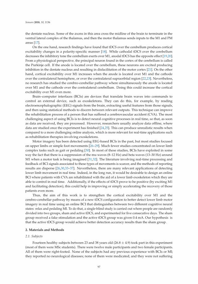
Sensors 2018, 18, 1136

the dentate nucleus. Some of the axons in this area cross the midline of the brain to terminate in theventral lateral complex of the thalamus, and then the motor thalamus sends inputs to the M1 and PMareas [17].

On the one hand, research findings have found that tDCS over the cerebellum produces corticalexcitability changes in a polarity-specific manner [18]. While cathodal tDCS over the cerebellumdecreases the inhibitory tone the cerebellum exerts over M1, anodal tDCS has the opposite effect [19,20].From a physiological perspective, the principal neuron found in the cortex of the cerebellum is calledthe Purkinje cell. If the anode is located over the cerebellum, these neurons are excited producinginhibition in the dentate nucleus and resulting in disfacilitation of the motor cortex [21]. On the otherhand, cortical excitability over M1 increases when the anode is located over M1 and the cathodeover the contralateral hemisphere, or over the contralateral supraorbital region [22,23]. Nevertheless,no research has studied the cerebro-cerebellar pathway where simultaneously the anode is locatedover M1 and the cathode over the contralateral cerebellum. Doing this could increase the corticalexcitability over M1 even more.

Brain–computer interfaces (BCIs) are devices that translate brain waves into commands tocontrol an external device, such as exoskeletons. They can do this, for example, by readingelectroencephalographic (EEG) signals from the brain, extracting useful features from those signals,and then using statistical methods to discern between relevant outputs. This technique can improvethe rehabilitation process of a person that has suffered a cerebrovascular accident (CVA). The mostchallenging aspect of using BCIs is to detect neural cognitive processes in real time, so that, as soonas data are received, they are processed. However, researchers usually analyze data offline, wheredata are studied once the experiment has finished [24,25]. This can produce unrealistic results whencompared to a more challenging online analysis, which is more relevant for real-time applications suchas rehabilitation therapies involving exoskeletons.

Motor imagery has been detected using EEG-based BCIs in the past, but most studies focusedon upper limbs or simple foot movements [26–29]. Much fewer studies concentrated on lower limbcomplex tasks such as gait or pedaling [30]. In most of these studies, BCIs have exploited in someway the fact that there is a suppression of the mu waves (8–12 Hz) and beta waves (13–30 Hz) aroundM1 when a motor task is being imagined [31,32]. The literature involving real-time processing andfeedback of BCI signals associated to these types of movements is scarcer, and the methods of reportingresults are disperse [26,30,33–37]. Nevertheless, there are many relevant applications of detectinglower limb movement in real time. Indeed, in the long run, it would be desirable to design an onlineBCI where patients with CVA are rehabilitated with the aid of a lower limb exoskeleton which they areable to control in real time. Additionally, if the effects of tDCS prove to be positive (by exciting M1and facilitating detection), this could help in improving or simply accelerating the recovery of thosepatients even more.

Thus, the aim of this work is to strengthen the cortical excitability over M1 and thecerebro-cerebellar pathway by means of a new tDCS configuration to better detect lower limb motorimagery in real time using an online BCI that distinguishes between two different cognitive neuralstates: relax and pedaling MI. To do that, a single-blind study is carried out where people are randomlydivided into two groups, sham and active tDCS, and experimented for five consecutive days. The shamgroup received a fake stimulation and the active tDCS group was given 0.4 mA. Our hypothesis isthat the active tDCS group would achieve better detection accuracy results than the sham group.

2. Materials and Methods

2.1. Subjects

Fourteen healthy subjects between 23 and 38 years old (26.8 ± 4.9) took part in this experiment(most of them were MSc students). There were twelve male participants and two female participants.All of them were right-footed. None of the subjects had any previous experience with BCIs or MI;they reported no neurological diseases; none of them were medicated; and they were not suffering

97

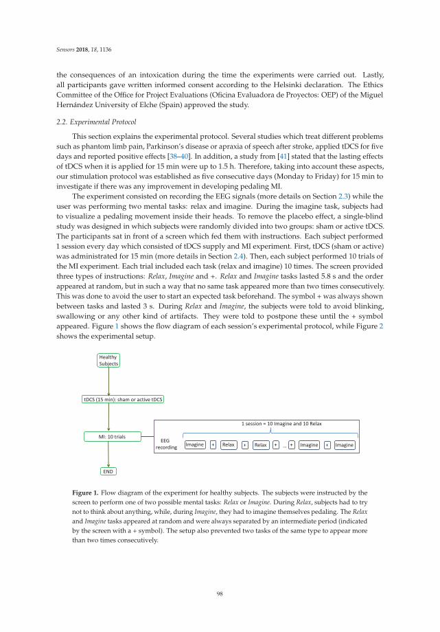
Sensors 2018, 18, 1136

the consequences of an intoxication during the time the experiments were carried out. Lastly,all participants gave written informed consent according to the Helsinki declaration. The EthicsCommittee of the Office for Project Evaluations (Oficina Evaluadora de Proyectos: OEP) of the MiguelHernández University of Elche (Spain) approved the study.

2.2. Experimental Protocol

This section explains the experimental protocol. Several studies which treat different problemssuch as phantom limb pain, Parkinson’s disease or apraxia of speech after stroke, applied tDCS for fivedays and reported positive effects [38–40]. In addition, a study from [41] stated that the lasting effectsof tDCS when it is applied for 15 min were up to 1.5 h. Therefore, taking into account these aspects,our stimulation protocol was established as five consecutive days (Monday to Friday) for 15 min toinvestigate if there was any improvement in developing pedaling MI.

The experiment consisted on recording the EEG signals (more details on Section 2.3) while theuser was performing two mental tasks: relax and imagine. During the imagine task, subjects hadto visualize a pedaling movement inside their heads. To remove the placebo effect, a single-blindstudy was designed in which subjects were randomly divided into two groups: sham or active tDCS.The participants sat in front of a screen which fed them with instructions. Each subject performed1 session every day which consisted of tDCS supply and MI experiment. First, tDCS (sham or active)was administrated for 15 min (more details in Section 2.4). Then, each subject performed 10 trials ofthe MI experiment. Each trial included each task (relax and imagine) 10 times. The screen providedthree types of instructions: Relax, Imagine and +. Relax and Imagine tasks lasted 5.8 s and the orderappeared at random, but in such a way that no same task appeared more than two times consecutively.This was done to avoid the user to start an expected task beforehand. The symbol + was always shownbetween tasks and lasted 3 s. During Relax and Imagine, the subjects were told to avoid blinking,swallowing or any other kind of artifacts. They were told to postpone these until the + symbolappeared. Figure 1 shows the flow diagram of each session’s experimental protocol, while Figure 2shows the experimental setup.

Healthy

Subjects

tDCS (15 min): sham or active tDCS

MI: 10 trials

END

Imagine Relax + + Relax + Imagine … + Imagine +

1 session = 10 Imagine and 10 Relax

EEG

recording

Figure 1. Flow diagram of the experiment for healthy subjects. The subjects were instructed by thescreen to perform one of two possible mental tasks: Relax or Imagine. During Relax, subjects had to trynot to think about anything, while, during Imagine, they had to imagine themselves pedaling. The Relax

and Imagine tasks appeared at random and were always separated by an intermediate period (indicatedby the screen with a + symbol). The setup also prevented two tasks of the same type to appear morethan two times consecutively.

98

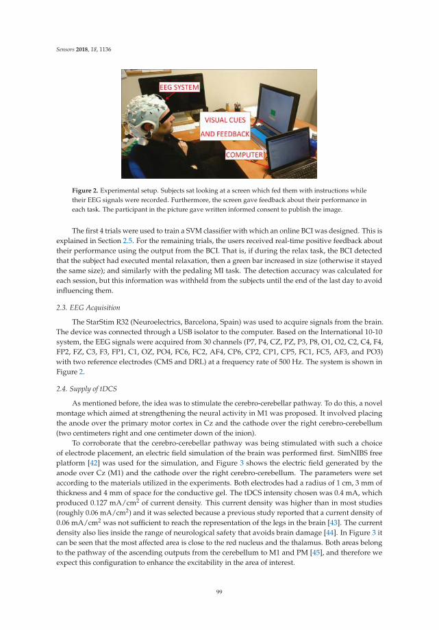
Sensors 2018, 18, 1136

Figure 2. Experimental setup. Subjects sat looking at a screen which fed them with instructions whiletheir EEG signals were recorded. Furthermore, the screen gave feedback about their performance ineach task. The participant in the picture gave written informed consent to publish the image.

The first 4 trials were used to train a SVM classifier with which an online BCI was designed. This isexplained in Section 2.5. For the remaining trials, the users received real-time positive feedback abouttheir performance using the output from the BCI. That is, if during the relax task, the BCI detectedthat the subject had executed mental relaxation, then a green bar increased in size (otherwise it stayedthe same size); and similarly with the pedaling MI task. The detection accuracy was calculated foreach session, but this information was withheld from the subjects until the end of the last day to avoidinfluencing them.

2.3. EEG Acquisition

The StarStim R32 (Neuroelectrics, Barcelona, Spain) was used to acquire signals from the brain.The device was connected through a USB isolator to the computer. Based on the International 10-10system, the EEG signals were acquired from 30 channels (P7, P4, CZ, PZ, P3, P8, O1, O2, C2, C4, F4,FP2, FZ, C3, F3, FP1, C1, OZ, PO4, FC6, FC2, AF4, CP6, CP2, CP1, CP5, FC1, FC5, AF3, and PO3)with two reference electrodes (CMS and DRL) at a frequency rate of 500 Hz. The system is shown inFigure 2.

2.4. Supply of tDCS

As mentioned before, the idea was to stimulate the cerebro-cerebellar pathway. To do this, a novelmontage which aimed at strengthening the neural activity in M1 was proposed. It involved placingthe anode over the primary motor cortex in Cz and the cathode over the right cerebro-cerebellum(two centimeters right and one centimeter down of the inion).

To corroborate that the cerebro-cerebellar pathway was being stimulated with such a choiceof electrode placement, an electric field simulation of the brain was performed first. SimNIBS freeplatform [42] was used for the simulation, and Figure 3 shows the electric field generated by theanode over Cz (M1) and the cathode over the right cerebro-cerebellum. The parameters were setaccording to the materials utilized in the experiments. Both electrodes had a radius of 1 cm, 3 mm ofthickness and 4 mm of space for the conductive gel. The tDCS intensity chosen was 0.4 mA, whichproduced 0.127 mA/cm2 of current density. This current density was higher than in most studies(roughly 0.06 mA/cm2) and it was selected because a previous study reported that a current density of0.06 mA/cm2 was not sufficient to reach the representation of the legs in the brain [43]. The currentdensity also lies inside the range of neurological safety that avoids brain damage [44]. In Figure 3 itcan be seen that the most affected area is close to the red nucleus and the thalamus. Both areas belongto the pathway of the ascending outputs from the cerebellum to M1 and PM [45], and therefore weexpect this configuration to enhance the excitability in the area of interest.

99

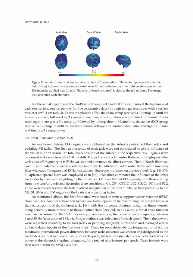
Sensors 2018, 18, 1136

Figure 3. Axial, coronal and sagital view of the tDCS simulation. The scale represents the electricfield (V/m) induced by the anode located over Cz and cathode over the right cerebro-cerebellum.The intensity applied was 0.4 mA. The most affected area (red) is close to the red nucleus. The imagewas generated with SimNIBS.

For the actual experiment, the StartStim R32 supplied anodal tDCS for 15 min at the beginning ofeach session (one session per day for five consecutive days) through two gel electrodes with a surfacearea of π cm2 (1 cm radius). To create a placebo effect, the sham group received a 3 s ramp up until theintensity chosen, followed by 3 s ramp down; then, no stimulation was provided for almost 15 minuntil again there was a 3 s ramp up followed by a ramp down. Meanwhile, the active tDCS groupreceived a 3 s ramp up until the intensity chosen, followed by constant stimulation throughout 15 min,and finally a 3 s ramp down.

2.5. Brain–Computer Interface (BCI)

As mentioned before, EEG signals were obtained as the subjects performed their relax andpedaling MI tasks. The first two seconds of each task were not considered to avoid influence ofthe visual cue and assure the total concentration of the subject in the respective task. Signals wereprocessed in 1 s epochs with a 200 ms shift. For each epoch, a 4th order Butterworth high-pass filterwith a cut-off frequency of 0.05 Hz was applied to remove the direct current. Then, a Notch filter wasused to eliminate the power line interference at 50 Hz. Afterward, a 4th order Butterworth low-passfilter with cut-off frequency of 45 Hz was utilized. Subsequently, based on previous work (e.g., [46,47]),a Laplacian spacial filter was employed as in [48]. This filter eliminates the influence of the otherelectrodes by means of weighting by their distance. Of these filtered EEG signals, only those comingfrom nine carefully selected electrodes were considered: Cz, CP1, CP2, C1, C2, C3, C4, FC1 and FC2.These were chosen because the task involved imagination of the lower limbs, so their proximity to theM1, S1, SMA and PM regions of the brain was a deciding factor.

As mentioned above, the first four trials were used to train a support vector machine (SVM)classifier. This classifier is based on hyperplane tasks separation by maximizing the margin betweenthe nearest points of the different tasks [49], with the outcomes obtained using non linear kernelsbeing generally more robust than those of other classifiers [50]. In this work, a radial basis functionwas used as kernel for the SVM. For every given electrode, the power at each frequency between6 and 30 Hz (resolution of 1 Hz via Burg’s method) was calculated for each epoch. Then, the powerswere separated according to the task (relax or pedaling imagery), normalized and averaged acrossall task-related epochs of the first four trials. Then, for each electrode, the frequency for which themaximum (normalized) power difference between tasks occurred was chosen and designated as theelectrode’s optimal frequency. Lastly, for each epoch, the feature associated to each electrode was thepower at the electrode’s optimal frequency, for a total of nine features per epoch. These features werethen used to train the SVM classifier.

100

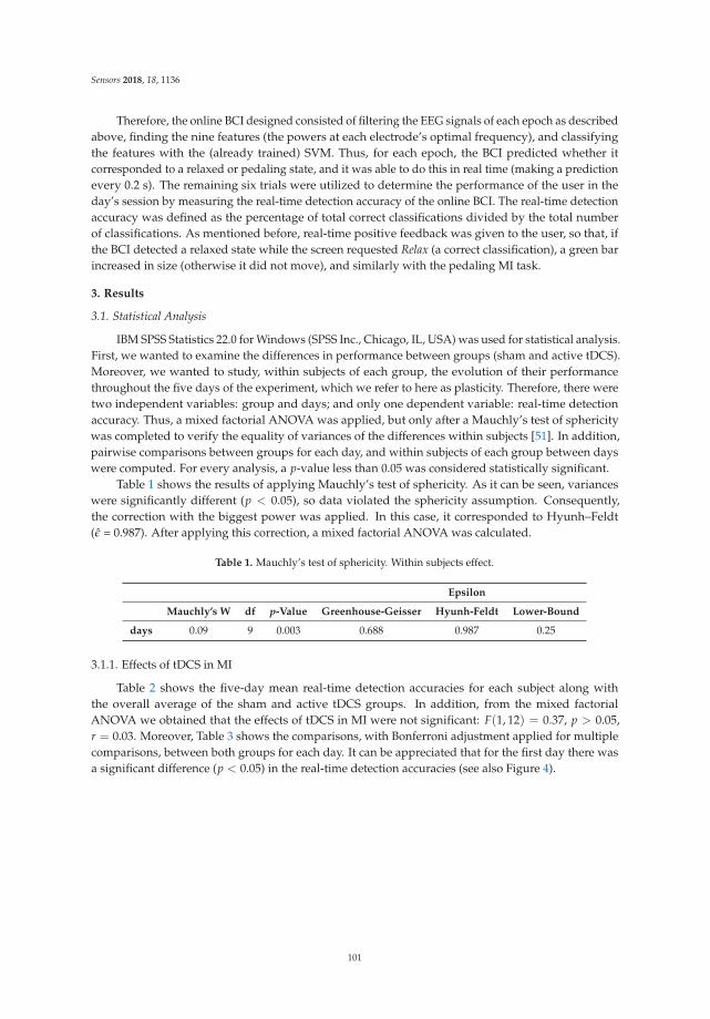
Sensors 2018, 18, 1136

Therefore, the online BCI designed consisted of filtering the EEG signals of each epoch as describedabove, finding the nine features (the powers at each electrode’s optimal frequency), and classifyingthe features with the (already trained) SVM. Thus, for each epoch, the BCI predicted whether itcorresponded to a relaxed or pedaling state, and it was able to do this in real time (making a predictionevery 0.2 s). The remaining six trials were utilized to determine the performance of the user in theday’s session by measuring the real-time detection accuracy of the online BCI. The real-time detectionaccuracy was defined as the percentage of total correct classifications divided by the total numberof classifications. As mentioned before, real-time positive feedback was given to the user, so that, ifthe BCI detected a relaxed state while the screen requested Relax (a correct classification), a green barincreased in size (otherwise it did not move), and similarly with the pedaling MI task.

3. Results

3.1. Statistical Analysis

IBM SPSS Statistics 22.0 for Windows (SPSS Inc., Chicago, IL, USA) was used for statistical analysis.First, we wanted to examine the differences in performance between groups (sham and active tDCS).Moreover, we wanted to study, within subjects of each group, the evolution of their performancethroughout the five days of the experiment, which we refer to here as plasticity. Therefore, there weretwo independent variables: group and days; and only one dependent variable: real-time detectionaccuracy. Thus, a mixed factorial ANOVA was applied, but only after a Mauchly’s test of sphericitywas completed to verify the equality of variances of the differences within subjects [51]. In addition,pairwise comparisons between groups for each day, and within subjects of each group between dayswere computed. For every analysis, a p-value less than 0.05 was considered statistically significant.

Table 1 shows the results of applying Mauchly’s test of sphericity. As it can be seen, varianceswere significantly different (p < 0.05), so data violated the sphericity assumption. Consequently,the correction with the biggest power was applied. In this case, it corresponded to Hyunh–Feldt(ǫ = 0.987). After applying this correction, a mixed factorial ANOVA was calculated.

Table 1. Mauchly’s test of sphericity. Within subjects effect.

Epsilon

Mauchly’s W df p-Value Greenhouse-Geisser Hyunh-Feldt Lower-Bound

days 0.09 9 0.003 0.688 0.987 0.25

3.1.1. Effects of tDCS in MI

Table 2 shows the five-day mean real-time detection accuracies for each subject along withthe overall average of the sham and active tDCS groups. In addition, from the mixed factorialANOVA we obtained that the effects of tDCS in MI were not significant: F(1, 12) = 0.37, p > 0.05,r = 0.03. Moreover, Table 3 shows the comparisons, with Bonferroni adjustment applied for multiplecomparisons, between both groups for each day. It can be appreciated that for the first day there wasa significant difference (p < 0.05) in the real-time detection accuracies (see also Figure 4).

101

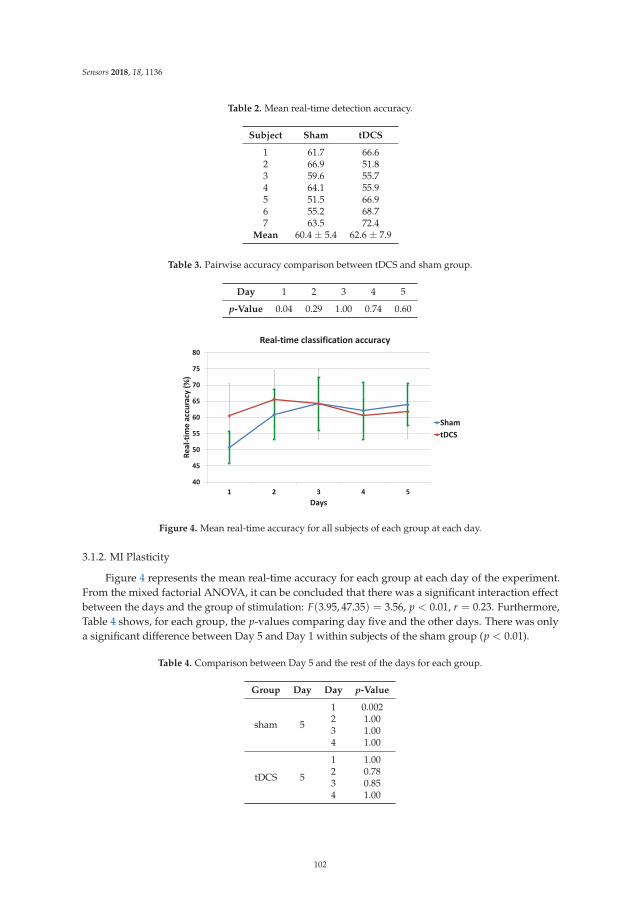
Sensors 2018, 18, 1136

Table 2. Mean real-time detection accuracy.

Subject Sham tDCS

1 61.7 66.62 66.9 51.83 59.6 55.74 64.1 55.95 51.5 66.96 55.2 68.77 63.5 72.4

Mean 60.4 ± 5.4 62.6 ± 7.9

Table 3. Pairwise accuracy comparison between tDCS and sham group.

Day 1 2 3 4 5

p-Value 0.04 0.29 1.00 0.74 0.60

40

45

50

55

60

65

70

75

80

1 2 3 4 5

Re

al-

tim

e a

ccu

racy

(%

)

Days

Real-time classification accuracy

Sham

tDCS

Figure 4. Mean real-time accuracy for all subjects of each group at each day.

3.1.2. MI Plasticity

Figure 4 represents the mean real-time accuracy for each group at each day of the experiment.From the mixed factorial ANOVA, it can be concluded that there was a significant interaction effectbetween the days and the group of stimulation: F(3.95, 47.35) = 3.56, p < 0.01, r = 0.23. Furthermore,Table 4 shows, for each group, the p-values comparing day five and the other days. There was onlya significant difference between Day 5 and Day 1 within subjects of the sham group (p < 0.01).

Table 4. Comparison between Day 5 and the rest of the days for each group.

Group Day Day p-Value

sham 5

1 0.0022 1.003 1.004 1.00

tDCS 5

1 1.002 0.783 0.854 1.00

102

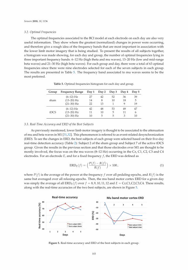
Sensors 2018, 18, 1136

3.2. Optimal Frequencies

The optimal frequencies associated to the BCI model at each electrode on each day are also veryuseful information. They show where the greatest (normalized) changes in power were occurring,and therefore give a rough idea of the frequency bands that are most important in association withthe lower limb motor imagery that is being studied. To present the results of all subjects together,a histogram was made showing, for each day and group, the number of optimal frequencies lying inthree important frequency bands: 6–12 Hz (high theta and mu waves), 13–20 Hz (low and mid-rangebeta waves) and 21–30 Hz (high beta waves). For each group and day, there were a total of 63 optimalfrequencies since there were nine electrodes selected for each of the seven subjects in each group.The results are presented in Table 5. The frequency band associated to mu waves seems to be themost preferred.

Table 5. Optimal frequencies histogram for each day and group.

Group Frequency Range Day 1 Day 2 Day 3 Day 4 Day 5

sham(6–12) Hz 27 42 52 36 39(13–20) Hz 14 8 10 18 5(21–30) Hz 22 13 1 9 19

tDCS(6–12) Hz 42 48 53 49 47(13–20) Hz 11 10 5 11 6(21–30) Hz 10 5 5 3 10

3.3. Real-Time Accuracy and ERD of the Best Subjects

As previously mentioned, lower limb motor imagery is thought to be associated to the attenuationof mu and beta waves in M1 [31,32]. This phenomenon is referred to as event-related desynchronization(ERD). To see the changes in ERD, the best subjects of each group were selected based on their five-dayreal-time detection accuracy (Table 2): Subject 2 of the sham group and Subject 7 of the active tDCSgroup. Given the results in the previous section and that those electrodes over M1 are thought to bemostly involved, the focus was on the mu waves (8–12 Hz) occurring in the Cz, C1, C2, C3 and C4electrodes. For an electrode E, and for a fixed frequency f , the ERD was defined as

ERDE( f ) =(P( f )− R( f )

R( f )

)× 100 , (1)

where P( f ) is the average of the power at the frequency f over all pedaling-epochs, and R( f ) is thesame but averaged over all relaxing-epochs. Then, the mu band motor cortex ERD for a given daywas simply the average of all ERDE( f ) over f = 8, 9, 10, 11, 12 and E = Cz,C1,C2,C3,C4. These results,along with the real-time accuracies of the two best subjects, are shown in Figure 5.

40

50

60

70

80

1 2 3 4 5

Re

al-

tim

e a

ccu

racy

(%

)

Days

Real-time accuracy

-50

-40

-30

-20

-10

00

1 2 3 4 5

ER

D (

%)

Mu band motor cortex ERD

Days

Figure 5. Real-time accuracy and ERD of the best subjects in each group.

103

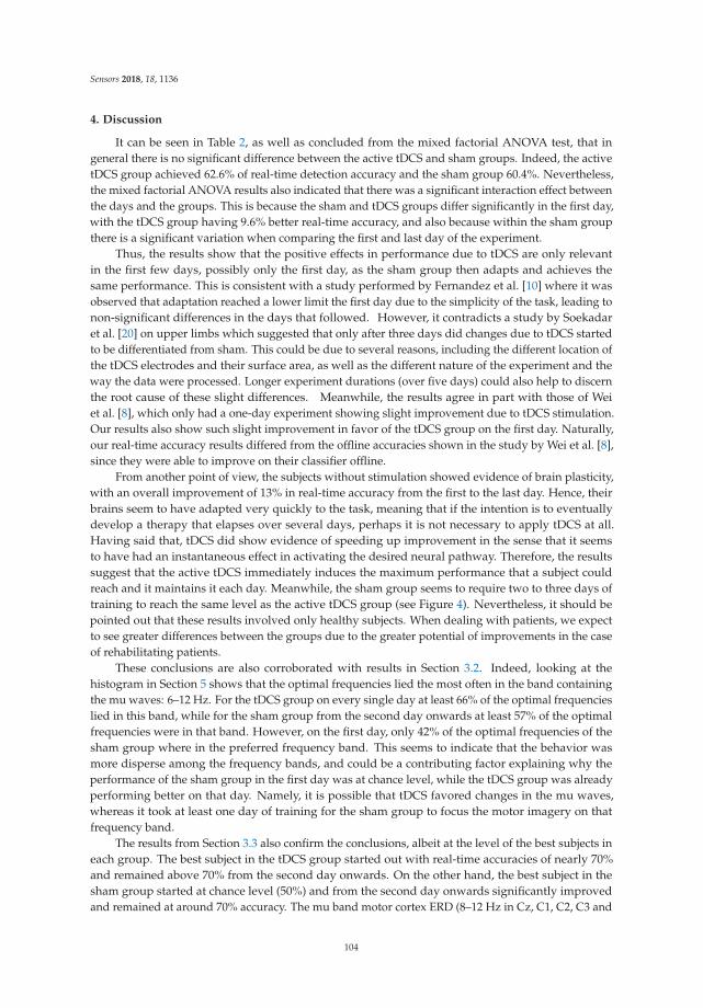
Sensors 2018, 18, 1136

4. Discussion

It can be seen in Table 2, as well as concluded from the mixed factorial ANOVA test, that ingeneral there is no significant difference between the active tDCS and sham groups. Indeed, the activetDCS group achieved 62.6% of real-time detection accuracy and the sham group 60.4%. Nevertheless,the mixed factorial ANOVA results also indicated that there was a significant interaction effect betweenthe days and the groups. This is because the sham and tDCS groups differ significantly in the first day,with the tDCS group having 9.6% better real-time accuracy, and also because within the sham groupthere is a significant variation when comparing the first and last day of the experiment.

Thus, the results show that the positive effects in performance due to tDCS are only relevantin the first few days, possibly only the first day, as the sham group then adapts and achieves thesame performance. This is consistent with a study performed by Fernandez et al. [10] where it wasobserved that adaptation reached a lower limit the first day due to the simplicity of the task, leading tonon-significant differences in the days that followed. However, it contradicts a study by Soekadaret al. [20] on upper limbs which suggested that only after three days did changes due to tDCS startedto be differentiated from sham. This could be due to several reasons, including the different location ofthe tDCS electrodes and their surface area, as well as the different nature of the experiment and theway the data were processed. Longer experiment durations (over five days) could also help to discernthe root cause of these slight differences. Meanwhile, the results agree in part with those of Weiet al. [8], which only had a one-day experiment showing slight improvement due to tDCS stimulation.Our results also show such slight improvement in favor of the tDCS group on the first day. Naturally,our real-time accuracy results differed from the offline accuracies shown in the study by Wei et al. [8],since they were able to improve on their classifier offline.

From another point of view, the subjects without stimulation showed evidence of brain plasticity,with an overall improvement of 13% in real-time accuracy from the first to the last day. Hence, theirbrains seem to have adapted very quickly to the task, meaning that if the intention is to eventuallydevelop a therapy that elapses over several days, perhaps it is not necessary to apply tDCS at all.Having said that, tDCS did show evidence of speeding up improvement in the sense that it seemsto have had an instantaneous effect in activating the desired neural pathway. Therefore, the resultssuggest that the active tDCS immediately induces the maximum performance that a subject couldreach and it maintains it each day. Meanwhile, the sham group seems to require two to three days oftraining to reach the same level as the active tDCS group (see Figure 4). Nevertheless, it should bepointed out that these results involved only healthy subjects. When dealing with patients, we expectto see greater differences between the groups due to the greater potential of improvements in the caseof rehabilitating patients.

These conclusions are also corroborated with results in Section 3.2. Indeed, looking at thehistogram in Section 5 shows that the optimal frequencies lied the most often in the band containingthe mu waves: 6–12 Hz. For the tDCS group on every single day at least 66% of the optimal frequencieslied in this band, while for the sham group from the second day onwards at least 57% of the optimalfrequencies were in that band. However, on the first day, only 42% of the optimal frequencies of thesham group where in the preferred frequency band. This seems to indicate that the behavior wasmore disperse among the frequency bands, and could be a contributing factor explaining why theperformance of the sham group in the first day was at chance level, while the tDCS group was alreadyperforming better on that day. Namely, it is possible that tDCS favored changes in the mu waves,whereas it took at least one day of training for the sham group to focus the motor imagery on thatfrequency band.

The results from Section 3.3 also confirm the conclusions, albeit at the level of the best subjects ineach group. The best subject in the tDCS group started out with real-time accuracies of nearly 70%and remained above 70% from the second day onwards. On the other hand, the best subject in thesham group started at chance level (50%) and from the second day onwards significantly improvedand remained at around 70% accuracy. The mu band motor cortex ERD (8–12 Hz in Cz, C1, C2, C3 and

104

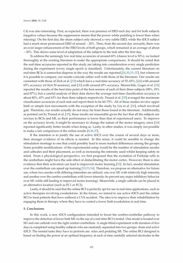
Sensors 2018, 18, 1136

C4) was also interesting. First, as expected, there was presence of ERD each day and for both subjects(negative values because the suppression means that the power while pedaling is lower than whenrelaxing). On the first day, the sham subject only showed a very subtle ERD, while the tDCS subjecthad a much more pronounced ERD of around −20%. Then, from the second day onwards, there wasan even larger enhancement of the ERD levels of both groups, which remained at an average of about−30%. This shows some level of adaptation of the subjects to the task after the first day.

To address the seemingly low real-time accuracies of around 60% (chance level is 50%), we lookedthoroughly at the existing literature to make the appropriate comparisons. It should be noted thatthe real-time accuracies reported in this study are taking into consideration every single predictionduring the experiment (every single epoch is classified). Unfortunately, the current literature onreal-time BCIs is somewhat disperse in the way the results are reported [26,30,33–37], but wheneverit is possible to compare, our results coincide rather well with those of the literature. Our results areconsistent with those of Zich et al. [33] which have a real-time accuracy of 55–65%, [26] with around65% accuracy (of first 30 sessions), and [30] with around 65% accuracy. Meanwhile, Guger et al. [34]reported the results of the best time point of the best session of each of their three subjects (98%, 93%and 87%), but a careful analysis of their data shows the average real-time classification accuracy isabout 80%, 65% and 65% for their three subjects respectively. Prasad et al. [35] averaged the maximumclassification accuracies of each task and report them to be 60–75%. All of these studies involve upperlimb or simple foot movements with the exception of the study by Liu et al. [30], which involvedgait. Therefore, our results actually do not stray far from those found in the literature. Additionally,as pointed out by Prasad et al. [35], these results are reasonable given the fact that all the subjects arenovices to BCIs and MI, so their performance is lower than that of experienced users. To improveon the accuracy levels, it might be necessary to change the nature of the motor imagery, since [26]reported significantly better results when doing so. Lastly, in other studies, it was simply not possibleto make a fair comparison of the online results [8,36,37].

If the intention is to justify the use of active tDCS over the course of several days or more,then stronger evidence of its effects is needed. In this sense, it could be sensible to change thestimulation montage to one that could possibly lead to more marked differences among the groups.Some possible modifications of the experimental setup would be the number of stimulation anodesand cathodes and their placement, as well as increasing the intensity used whilst keeping safety inmind. From a physiological perspective, we first proposed that the excitation of Purkinje cells inthe cerebellum might have the side effect of disfacilitating the motor cortex. However, there is alsoevidence that their activation can lead to improved motor learning [52]. In fact, anodal stimulationover the cerebellum can speed up learning [19,53,54]. Therefore, we propose an alternative for futureuse, where two anodes with differing intensities are utilized: one over M1 with relatively high intensity,and another over the cerebro-cerebellum with lower intensity (to prevent any major inhibitory behaviorover M1 while still leading to improved motor learning). Meanwhile, a single cathode can be placed inan alternative location (such as FC1 or FC2).

Lastly, it should be said that the online BCI is perfectly apt for use in real-time applications, such asactive therapies involving exoskeletons. In the future, we intend to use active tDCS and the onlineBCI to treat patients that have suffered a CVA accident. The idea is to improve their rehabilitation byengaging them in therapy where they have to control a lower limb exoskeleton in real time.

5. Conclusions

In this work, a new tDCS configuration intended to boost the cerebro-cerebellar pathway toimprove the detection of lower limb MI via the use of a real-time BCI is tested. One anode is located overM1 and one cathode over the right cerebro-cerebellum. A single-blind experiment with duration of fivedays is completed using healthy subjects who are randomly separated into two groups: sham and activetDCS. The mental tasks they have to perform are: relax and pedaling MI. The online BCI designed isbased on finding the power at an optimal frequency at each of nine carefully selected electrodes in the

105

Sensors 2018, 18, 1136

proximity of M1, S1, PM and SMA. From the very first day, the real-time detection accuracy achievedby the active tDCS group is over 60% and remains around 62.6% on average. However, the sham groupneeds three days of training to reach that same level of accuracy. This, along with other supportingevidence, indicates possibly that the tDCS has an immediate effect in activating the desired neuralpathway, and shows the potential advantages in accelerating recovery of patients undergoing therapy.However, overall, the long-term effects of tDCS seems to have been moderate at best. With this inmind, the stimulation montage could possibly be further improved to increase the effects of tDCSand hopefully justify its use. Lastly, the online BCI designed, with or without tDCS, is a desirablestepping stone in designing therapies that allow recovering patients’ real-time control of lower limbexoskeletons, which is a future endeavor of interest.

Acknowledgments: This research was carried out in the framework of the project Associate titled: Decodingand stimulation of motor and sensory brain activity to support long term potentiation through Hebbian andpaired associative stimulation during rehabilitation of gait (DPI2014-58431-C4-2-R), which is funded by theSpanish Ministry of Economy and Competitiveness and by the European Union through the European RegionalDevelopment Fund (ERDF), “A way to build Europe”. M. Rodríguez-Ugarte wishes to thank Federico Fuentes foruseful discussions and the careful revision of the manuscript. Lastly, the authors wish to thank the reviewers forthe helpful comments that significantly improved the quality of the manuscript.

Author Contributions: M.d.l.S.R.-U. is responsible for the design, implementation, acquisition and data analysis.In addition, E.I. and M.O.-G. supervised the work and contributed with the revision process. J.M.A. activelycontributed as director of the work.

Conflicts of Interest: The authors declare no conflict of interest.

Abbreviations

The following abbreviations are used in this manuscript:

CVA Cerebrovascular accidentMI Motor imagerytDCS Transcranial direct current stimulationBCI Brain–computer interfaceM1 Primary motor cortexS1 Primary somatosensory cortexSMA Supplementary motor areaPM PremotorEEG ElectroencephalographicSVM Support vector machineERD Event-related desynchronization

References

1. Kumru, H.; Murillo, N.; Benito-Penalva, J.; Tormos, J.M.; Vidal, J. Transcranial direct current stimulation isnot effective in the motor strength and gait recovery following motor incomplete spinal cord injury duringLokomat R© gait training. Neurosci. Lett. 2016, 620, 143–147.

2. Flöel, A. tDCS-enhanced motor and cognitive function in neurological diseases. Neuroimage 2014, 85, 934–947.3. Chieffo, R.; Ciocca, M.; Leocani, L.; Miranda, P.; Rothwell, J. 113. Short-term effect of different tdcs intensities

on motor cortex excitability. Clin. Neurophysiol. 2015, 126, e26.4. Batsikadze, G.; Moliadze, V.; Paulus, W.; Kuo, M.F.; Nitsche, M. Partially non-linear stimulation

intensity-dependent effects of direct current stimulation on motor cortex excitability in humans. J. Physiol.

2013, 591, 1987–2000.5. Bai, S.; Dokos, S.; Ho, K.A.; Loo, C. A computational modelling study of transcranial direct current

stimulation montages used in depression. Neuroimage 2014, 87, 332–344.6. Lee, S.J.; Chun, M.H. Combination transcranial direct current stimulation and virtual reality therapy for

upper extremity training in patients with subacute stroke. Arch. Phys. Med. Rehabil. 2014, 95, 431–438.

106

Sensors 2018, 18, 1136

7. Achilles, E.; Weiss-Blankenhorn, P.; Moos, K.; Hesse, M.; Sparing, R.; Fink, G. P649: Transcranial direct currentstimulation (tDCS) of left parietal cortex facilitates gesture processing in healthy subjects. Clin. Neurophysiol.

2014, 125, S226–S227.8. Wei, P.; He, W.; Zhou, Y.; Wang, L. Performance of motor imagery brain-computer interface based on anodal

transcranial direct current stimulation modulation. IEEE Trans. Neural Syst. Rehabil. Eng. 2013, 21, 404–415.9. Shah, B.; Nguyen, T.T.; Madhavan, S. Polarity independent effects of cerebellar tDCS on short term ankle

visuomotor learning. Brain Stimul. 2013, 6, 966–968.10. Fernandez, L.; Albein-Urios, N.; Kirkovski, M.; McGinley, J.L.; Murphy, A.T.; Hyde, C.; Stokes, M.A.;

Rinehart, N.J.; Enticott, P.G. Cathodal transcranial direct current stimulation (tDCS) to the right cerebellarhemisphere affects motor adaptation during gait. Cerebellum 2017, 16, 168–177.

11. Cevallos, C.; Zarka, D.; Hoellinger, T.; Leroy, A.; Dan, B.; Cheron, G. Oscillations in the human brain duringwalking execution, imagination and observation. Neuropsychologia 2015, 79, 223–232.

12. Sahyoun, C.; Floyer-Lea, A.; Johansen-Berg, H.; Matthews, P. Towards an understanding of gait control:Brain activation during the anticipation, preparation and execution of foot movements. Neuroimage 2004,21, 568–575.

13. Fukuyama, H.; Ouchi, Y.; Matsuzaki, S.; Nagahama, Y.; Yamauchi, H.; Ogawa, M.; Kimura, J.; Shibasaki, H.Brain functional activity during gait in normal subjects: A SPECT study. Neurosci. Lett. 1997, 228, 183–186.

14. Solodkin, A.; Hlustik, P.; Chen, E.E.; Small, S.L. Fine modulation in network activation during motorexecution and motor imagery. Cerebral Cortex 2004, 14, 1246–1255.

15. Parsons, L.M.; Fox, P.T.; Downs, J.H.; Glass, T.; Hirsch, T.B.; Martin, C.C.; Jerabek, P.A.; Lancaster, J.L. Use ofimplicit motor imagery for visual shape discrimination as revealed by PET. Nature 1995, 375, 54–58.

16. D’Angelo, E.; Casali, S. Seeking a unified framework for cerebellar function and dysfunction: from circuitoperations to cognition. Front. Neural Circ. 2012, 6, doi:10.3389/fncir.2012.00116.

17. Penhune, V.B.; Steele, C.J. Parallel contributions of cerebellar, striatal and M1 mechanisms to motor sequencelearning. Behav. Brain Res. 2012, 226, 579–591.

18. Galea, J.M.; Jayaram, G.; Ajagbe, L.; Celnik, P. Modulation of cerebellar excitability by polarity-specificnoninvasive direct current stimulation. J. Neurosci. 2009, 29, 9115–9122.

19. Block, H.J.; Celnik, P. Can cerebellar transcranial direct current stimulation become a valuableneurorehabilitation intervention? Expert Rev. Neurother. 2012, 12, 1275–1277.

20. Soekadar, S.R.; Witkowski, M.; Birbaumer, N.; Cohen, L.G. Enhancing Hebbian learning to control brainoscillatory activity. Cerebral Cortex 2014, 25, 2409–2415.

21. Cengiz, B.; Boran, H.E. The role of the cerebellum in motor imagery. Neurosci. Lett. 2016, 617, 156–159.22. Wagner, T.; Fregni, F.; Fecteau, S.; Grodzinsky, A.; Zahn, M.; Pascual-Leone, A. Transcranial direct current

stimulation: A computer-based human model study. Neuroimage 2007, 35, 1113–1124.23. Sehm, B.; Kipping, J.; Schäfer, A.; Villringer, A.; Ragert, P. A comparison between uni-and bilateral

tDCS effects on functional connectivity of the human motor cortex. Front. Hum. Neurosci. 2013, 7,doi:10.3389/fnhum.2013.00183.

24. Pfurtscheller, G.; Brunner, C.; Schlögl, A.; Da Silva, F.L. Mu rhythm (de) synchronization and EEG single-trialclassification of different motor imagery tasks. NeuroImage 2006, 31, 153–159.

25. Lew, E.; Chavarriaga, R.; Silvoni, S.; Millán, J.d.R. Detection of self-paced reaching movement intention fromEEG signals. Front. Neuroeng. 2012, 5, doi:10.3389/fneng.2012.00013.

26. Pfurtscheller, G.; Neuper, C. Motor imagery and direct brain-computer communication. Proc. IEEE 2001,89, 1123–1134.

27. Cincotti, F.; Mattia, D.; Aloise, F.; Bufalari, S.; Schalk, G.; Oriolo, G.; Cherubini, A.; Marciani, M.G.; Babiloni, F.Non-invasive brain–computer interface system: Towards its application as assistive technology. Brain Res.

Bull. 2008, 75, 796–803.28. Müller-Putz, G.R.; Kaiser, V.; Solis-Escalante, T.; Pfurtscheller, G. Fast set-up asynchronous brain-switch

based on detection of foot motor imagery in 1-channel EEG. Med. Biol. Eng. Comput. 2010, 48, 229–233.29. Ang, K.K.; Guan, C.; Chua, K.S.G.; Ang, B.T.; Kuah, C.W.K.; Wang, C.; Phua, K.S.; Chin, Z.Y.; Zhang, H.

A large clinical study on the ability of stroke patients to use an EEG-based motor imagery brain-computerinterface. Clin. EEG Neurosci. 2011, 42, 253–258.

107

Sensors 2018, 18, 1136

30. Liu, D.; Chen, W.; Lee, K.; Pei, Z.; Millán, J.d.R. An EEG-based brain-computer interface for gait training.In Proceedings of the 2017 29th Chinese Control And Decision Conference (CCDC), Chongqing, China,28–30 May 2017; pp. 6755–6760.

31. Pfurtscheller, G.; Neuper, C. Motor imagery activates primary sensorimotor area in humans. Neurosci. Lett.

1997, 239, 65–68.32. Naros, G.; Naros, I.; Grimm, F.; Ziemann, U.; Gharabaghi, A. Reinforcement learning of self-regulated

sensorimotor β-oscillations improves motor performance. Neuroimage 2016, 134, 142–152.33. Zich, C.; Debener, S.; Kranczioch, C.; Bleichner, M.G.; Gutberlet, I.; De Vos, M. Real-time EEG feedback during

simultaneous EEG–fMRI identifies the cortical signature of motor imagery. Neuroimage 2015, 114, 438–447.34. Guger, C.; Ramoser, H.; Pfurtscheller, G. Real-time EEG analysis with subject-specific spatial patterns for

a brain-computer interface (BCI). IEEE Trans. Rehabil. Eng. 2000, 8, 447–456.35. Prasad, G.; Herman, P.; Coyle, D.; McDonough, S.; Crosbie, J. Applying a brain-computer interface to support

motor imagery practice in people with stroke for upper limb recovery: A feasibility study. J. Neuroeng.

Rehabil. 2010, 7, 60.36. Yu, T.; Xiao, J.; Wang, F.; Zhang, R.; Gu, Z.; Cichocki, A.; Li, Y. Enhanced motor imagery training using

a hybrid BCI with feedback. IEEE Trans. Biomed. Eng. 2015, 62, 1706–1717.37. Horki, P.; Solis-Escalante, T.; Neuper, C.; Müller-Putz, G. Combined motor imagery and SSVEP based BCI

control of a 2 DoF artificial upper limb. Med. Biol. Eng. Comput. 2011, 49, 567–577.38. Bolognini, N.; Spandri, V.; Ferraro, F.; Salmaggi, A.; Molinari, A.C.; Fregni, F.; Maravita, A. Immediate and

sustained effects of 5-day transcranial direct current stimulation of the motor cortex in phantom limb pain.J. Pain 2015, 16, 657–665.

39. Ferrucci, R.; Mameli, F.; Ruggiero, F.; Priori, A. Transcranial direct current stimulation as treatment forParkinson’s disease and other movement disorders. Basal Ganglia 2016, 6, 53–61.

40. Marangolo, P.; Marinelli, C.; Bonifazi, S.; Fiori, V.; Ceravolo, M.; Provinciali, L.; Tomaiuolo, F.Electrical stimulation over the left inferior frontal gyrus (IFG) determines long-term effects in the recovery ofspeech apraxia in three chronic aphasics. Behav. Brain Res. 2011, 225, 498–504.

41. Nitsche, M.A.; Paulus, W. Sustained excitability elevations induced by transcranial DC motor cortexstimulation in humans. Neurology 2001, 57, 1899–1901.

42. Thielscher, A.; Antunes, A.; Saturnino, G.B. Field modeling for transcranial magnetic stimulation: A usefultool to understand the physiological effects of TMS? In Proceedings of the 2015 37th Annual InternationalConference of the IEEE Engineering in Medicine and Biology Society (EMBC), Milan, Italy, 25–29 August2015; pp. 222–225.

43. Angulo-Sherman, I.N.; Rodríguez-Ugarte, M.; Sciacca, N.; Iáñez, E.; Azorín, J.M. Effect of tDCS stimulationof motor cortex and cerebellum on EEG classification of motor imagery and sensorimotor band power.J. Neuroeng. Rehabil. 2017, 14, 31.

44. Antal, A.; Alekseichuk, I.; Bikson, M.; Brockmöller, J.; Brunoni, A.; Chen, R.; Cohen, L.; Dowthwaite, G.;Ellrich, J.; Flöel, A.; et al. Low intensity transcranial electric stimulation: Safety, ethical, legal regulatory andapplication guidelines. Clin. Neurophysiol. 2017, 128, 1774–1809.

45. Llinas, R.; Negrello, M.N. Cerebellum. Scholarpedia 2015, 10, 4606.46. Rodríguez-Ugarte, M.; Costa, Á.; Iáñez, E.; Úbeda, A.; Azorín, J. Pseudo-online detection of intention of

pedaling start cycle through EEG signals. In Converging Clinical and Engineering Research on Neurorehabilitation

II; Springer: New York, NY, USA, 2017; pp. 1103–1107.47. Hortal, E.; Úbeda, A.; Iáñez, E.; Azorín, J.M.; Fernández, E. EEG-Based Detection of Starting and Stopping

During Gait Cycle. Int. J. Neural Syst. 2016, 26, 1650029.48. McFarland, D.J.; McCane, L.M.; David, S.V.; Wolpaw, J.R. Spatial filter selection for EEG-based

communication. Electroencephalogr. Clin. Neurophysiol. 1997, 103, 386–394.49. Steinwart, I.; Christmann, A. Support Vector Machines; Springer Science & Business Media:

New York, NY, USA, 2008.50. Hamedi, M.; Salleh, S.H.; Noor, A.M.; Mohammad-Rezazadeh, I. Neural network-based three-class motor

imagery classification using time-domain features for BCI applications. In Proceedings of the Region 10Symposium, Kuala Lumpur, Malaysia, 14–16 April 2014; pp. 204–207.

51. Field, A. Discovering Statistics Using IBM SPSS Statistics; Sage: Thousand Oaks, CA, USA, 2013.

108

Sensors 2018, 18, 1136

52. Nguyen-Vu, T.B.; Kimpo, R.R.; Rinaldi, J.M.; Kohli, A.; Zeng, H.; Deisseroth, K.; Raymond, J.L.Cerebellar Purkinje cell activity drives motor learning. Nat. Neurosci. 2013, 16, 1734–1736.

53. Priori, A.; Ciocca, M.; Parazzini, M.; Vergari, M.; Ferrucci, R. Transcranial cerebellar direct current stimulationand transcutaneous spinal cord direct current stimulation as innovative tools for neuroscientists. J. Physiol.

2014, 592, 3345–3369.54. Grimaldi, G.; Manto, M. Anodal transcranial direct current stimulation (tDCS) decreases the amplitudes of

long-latency stretch reflexes in cerebellar ataxia. Ann. Biomed. Eng. 2013, 41, 2437–2447.

c© 2018 by the authors. Licensee MDPI, Basel, Switzerland. This article is an open accessarticle distributed under the terms and conditions of the Creative Commons Attribution(CC BY) license (http://creativecommons.org/licenses/by/4.0/).

109

sensors

Article

A Novel Feature Optimization for WearableHuman-Computer Interfaces Using SurfaceElectromyography Sensors

Han Sun, Xiong Zhang *, Yacong Zhao, Yu Zhang, Xuefei Zhong and Zhaowen Fan

Department of Electronic Science and Engineering, Southeast University, Nanjing 210096, China;230139593@seu.edu.cn (H.S.); 220161239@seu.edu.cn (Ya.Z.); 230129600@seu.edu.cn (Yu.Z.);zxf@seu.edu.cn (Xu.Z.); zhaowenfan@seu.edu.cn (Z.F.)* Correspondence: zxbell@seu.edu.cn; Tel.: +86-138-0903-3793

Received: 4 January 2018; Accepted: 13 March 2018; Published: 15 March 2018

Abstract: The novel human-computer interface (HCI) using bioelectrical signals as input is a valuabletool to improve the lives of people with disabilities. In this paper, surface electromyography (sEMG)signals induced by four classes of wrist movements were acquired from four sites on the lowerarm with our designed system. Forty-two features were extracted from the time, frequency andtime-frequency domains. Optimal channels were determined from single-channel classificationperformance rank. The optimal-feature selection was according to a modified entropy criteria (EC)and Fisher discrimination (FD) criteria. The feature selection results were evaluated by four differentclassifiers, and compared with other conventional feature subsets. In online tests, the wearablesystem acquired real-time sEMG signals. The selected features and trained classifier model wereused to control a telecar through four different paradigms in a designed environment with simpleobstacles. Performance was evaluated based on travel time (TT) and recognition rate (RR). The resultsof hardware evaluation verified the feasibility of our acquisition systems, and ensured signal quality.Single-channel analysis results indicated that the channel located on the extensor carpi ulnaris (ECU)performed best with mean classification accuracy of 97.45% for all movement’s pairs. Channelsplaced on ECU and the extensor carpi radialis (ECR) were selected according to the accuracy rank.Experimental results showed that the proposed FD method was better than other feature selectionmethods and single-type features. The combination of FD and random forest (RF) performed bestin offline analysis, with 96.77% multi-class RR. Online results illustrated that the state-machineparadigm with a 125 ms window had the highest maneuverability and was closest to real-life control.Subjects could accomplish online sessions by three sEMG-based paradigms, with average times of46.02, 49.06 and 48.08 s, respectively. These experiments validate the feasibility of proposed real-timewearable HCI system and algorithms, providing a potential assistive device interface for personswith disabilities.

Keywords: human-computer interface; surface electromyogram; channel selection; feature optimization;multi-class recognition; support vector machine

1. Introduction

Human-computer interfaces (HCI) for those with motor deficits based on bioelectrical signalshave received increasing attention in the last decade. HCI provides communication and controlchannels between human subjects and the surrounding environment with the purpose of replacementor augmentation of muscle activity [1]. Common classes of bio-signals used to control assistive devicesinclude electromyography (EMG) [2,3], electroencephalography (EEG) [4,5], electrooculography(EOG) [6,7], and fusions of these signals [8–11].

Sensors 2018, 18, 869; doi:10.3390/s18030869 www.mdpi.com/journal/sensors110

Sensors 2018, 18, 869

This work presents the performance results of an HCI system based on electrical currentsgenerated in the contraction and relaxation phase of muscles [12] known as sEMG. Measurement ofsEMG is noninvasive, can offer excellent signal-to-noise ratio compared to EEG, and provides real-timeinformation about muscle intents [13].

Applications of sEMG include early disease detection [14], seizure [15,16] and falldetection [10,17], gesture [18,19], and sign language recognition [3,20]. These applications recordedactivities of facial [21,22], upper [18,23] and lower-limb [17,24] muscles.

The sEMG-based HCIs are sensitive to electronic noise, movement artefacts and musclefatigue [12]. To overcome the problem, wearable rigid printed circuit board (PCB)-based systems areoften used [3,25,26]. However, these devices still need to be fully fixed and tethered. Another solutionis development of wearable and flexible electronics. These sEMG sensors have been utilized to monitorelectrocardiogram (ECG), EMG and body posture [27,28] signals as well as to detect arm gestures [29].

The sEMG-based HCIs require effective features to provide real-time efficiency from the dataprocessing standpoint. Time-domain feature extraction is the most common method because thesefeatures provide high recognition rate and low computational cost. Root mean square (RMS) [30–33]and mean absolute value (MAV) [29,33,34] are most popular among these features. Time-frequencydomain features which characterize varying frequency information at different time locations havereceived attention recently. Time-frequency domain analysis can efficiently eliminate the non-stationarynoise in either time or frequency domain [12,35–38].

Feature optimization/selection techniques further enhance the performance. These techniquesinclude filter, wrapper, and embedded methods [39]. Filter and wrapper methods havevery low computational costs because they optimize features independent of the classificationperformance [40,41]. In contrast, embedded methods rely on criteria that are generated during theclassifier training process. Examples of embedded techniques are the support vector machine(SVM)-based Recursive Feature Elimination (RFE) [42] and the linear discriminant analysis(LDA)-based Fisher’s Discriminant (FD) function [17].

Channel selection is another simple feature selection/optimization technique. Within this method,channel optimization is based on the single-channel classification accuracy. A more sophisticatedadaptation is about selecting important muscles/channels that highly contribute to the specificmovements according to the power and frequency distribution of sEMG signals [31].

Classification is the next step to distinguish between different movements. Simple and linearclassifiers are preferable because of their simplicity and ease of implementation. For example,Linear Discriminant Analysis (LDA) [29], k-Nearest Neighbor (kNN) [3] and Decision Tree (DT) [3,13]are feasible to separate small numbers of uncomplicated classes clearly. To increase expandabilityand performance in complicated systems, Support Vector Machine (SVM) [43], Artificial NeuralNetwork (ANN) [44], Fuzzy Min-Max Neural Network (FMMNN) [40] and Random Forest (RF) [37]are suggested for classification. Neural Network classifiers can be used for both simple and complexcases due to their high performance. However, with too many hidden layers or hidden units, theclassifiers need long training times and require large amounts of training data. Unsupervised learningmethods including K-Means and Fuzzy C-Means have also provided high classification performancein sEMG recognition [32].

An important application of biopotential-based HCI is smart wheelchair control. The conventionalparadigm of smart wheelchair control is through joysticks [45]. This paradigm is not applicable forpatients with low or no control of their upper limb. The sEMG-based HCI is an advanced alternativecontroller [46,47], however with more sophisticated implementation than the conventional joystickcontrol. A critical problem is the functionality requirement for accurate control. (1) The recognitionfor more motions or gestures can increase degree-of-freedom [37,42]. (2) A state-machine basedcontrol and a proportional control could meet the requirement [48,49]. In this method, a modality ora channel is used to switch control modes. (3) Fusion of two or more types of sensors can realize thehigh-dimensional control for assistive devices. The combination of sEMG and inertial measurement

111

Sensors 2018, 18, 869

units (IMU) consisted of conventional accelerometers (ACC) and gyroscopes is frequently used becauseof the high performance in long-term control. Muscle fatigue and skin sweat can make sEMG signalsdrift, while they have no influence to IMU signals [50,51].

In this paper, we explore the performance of sEMG-based HCI in controlling a telecar. We presenta wireless wearable sEMG system based on flexible printed circuit (FPC) with embedded dry metallicdetecting electrodes that avoids channels connection and fixation challenges. We also presentmethodology to select sEMG feature subsets for the recognition of four movements. The novelentropy criteria (EC) and Fisher discrimination (FD) criteria are compared with the conventional RFEmethod. Dunn-Heriksen et al. [52] introduced EC in EEG channel selection. Here we adopt EC forsEMG feature optimization. Fisher’s discriminant based separability measurement has been widelyutilized in feature optimization [17,40]. However, we introduce a novel method to compute the ratioof between-class distances to within-class distances. Finally, subjects control a designed telecar basedon different paradigms using the optimal channels and features.

The structure of this paper is as follows: Section 2 describes two types of sEMG acquisitionsystems. Experimental methods about anticipants, experiment design, sensors placement are discussedin Section 3. Signal processing techniques including preprocessing, feature extraction, selection, andclassification are explained in Section 4. Section 5 introduces four different control paradigms, followedby the results of offline analysis and real-time control in Section 6. Finally, Sections 7 and 8 discuss andconclude with the strengths of the current work.

2. System Architecture

The entire circuit structure of two types of sEMG acquisition systems consists of four main parts:a power module, a signal-conditioning module, a signal-processing module, and a signal-transmissionmodule. The power module provides required power and safety precaution for using in humanrecordings. The function of signal-conditioning module is to amplify and filter raw signals.Analog filtered sEMG signals are converted into digital signals in the signal-processing module.Finally, the signal-transmission module transmits these digital signals to PC. Our overall hardwaredesign includes the requirements of low cost, low power, small size, human compatibility, and ease ofprogramming and interfacing with standard computers.

2.1. Offline sEMG Acquisition System

We used disposable disc sensors in offline sEMG acquisition, as shown in Figure 1b. These sensorsconsist of Ag/AgCl electrodes, conductive gel, an adhesive area and a snap connection. Wet sensorswith conductive gel ensure an easy conversion between ionic current and electron current, resulting inlow electrode impedance up to few kilo-ohms [53]. Diameters of the Ag/AgCl electrodes, conductivegel, and disc sensors are 9, 15 and 34 mm, respectively. Two sensors, at a distance of roughly 30 mm,constitute a pair of bi-polar sEMG electrodes.

The sEMG signal has small amplitude and is severely distorted by electromagnetic interference.An approach to reduce the electrode-skin interference is to employ an amplifier with high inputimpedance. The acquisition system board presented in Figure 1a (32 × 22 mm2) includesa high-performance voltage follower (AD8626, Analog Devices, Norwood, MA, USA) as well asa differential amplifier (INA128, TI, Dallas, TX, USA) with very large input impedance. Togetherthey largely reduce common mode interference (CMI) as well as improve the common mode rejectionratio (CMRR) and signal to noise ratio (SNR). We further reduce differential mode interference (DMI)with anti-aliasing and on chip digital filters. In both hardware and software solutions, the high-passfilter may have a 3 dB cutoff frequency of 10–20 Hz and the low-pass filter a 3 dB cutoff frequencyof 400–450 Hz to avoid loss of information from the sEMG signals [54]. Therefore, a pass-band filterbetween 10 Hz to 450 Hz is designed using the AD8626. The sEMG signals are further passed througha notch filter at 50 Hz (UAF42, TI).

112

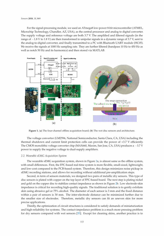
Sensors 2018, 18, 869

For the signal-processing module, we used an ATmega8 low-power 8-bit microcontroller (ATMEL,Microchip Technology, Chandler, AZ, USA), as the central processor and analog to digital converter.The supply voltage and reference voltage are both 3.7 V. The amplified and filtered signals (in therange of −1.8 V to 1.8 V) are then transformed to unipolar signals in a dynamic range of 3.7 V, sent tothe analog-to-digital converter, and finally transmitted to a PC with Bluetooth UART module (HC05).We receive the signals at 1000 Hz sampling rate. They are further filtered (bandpass 10 Hz to 450 Hz aswell as notch 50 Hz and its harmonics) and then stored via MATLAB.

(a)

(b)

Figure 1. (a) The four-channel offline acquisition board; (b) The wet disc sensors and architecture.

The voltage convertor (LM2596, National Semiconductor, Santa Clara, CA, USA) including thethermal shutdown and current limit protection cells can provide the power of +3.7 V efficiently.The CMOS monolithic voltage converter chip (MAX660, Maxim, San Jose, CA, USA) produces a −3.7 Vpower to supply the negative voltage to dual-supply amplifiers.

2.2. Wearable sEMG Acquisition System

The wearable sEMG acquisition system, shown in Figure 2a, is almost same as the offline system,with small differences. First, the FPC-based real-time system is more flexible, small-sized, lightweight,and low-cost compared to the PCB-based system. Therefore, this design minimizes noise pickup insEMG recording stations, and allows for recording without additional pre-amplification steps.

Second, in term of sensors materials, we designed two pairs of metallic dry sensors. This type ofdisc sensors is plated with copper on the top layer of FPC-based board. The next step is plating nickeland gold on the copper disc to stabilize contact impedance as shown in Figure 2b. Low electrode-skinimpedance is critical for recording high-quality signals. The traditional solution is to gently exfoliateskin using abrasive gel or 75% alcohol. The diameter of each sensor is 3 mm and the fixed distancewithin a pair of sensors is 30 mm. The inter-electrode distance can be minimized further due tothe smaller size of electrodes. Therefore, metallic dry sensors can fit an uneven skin for moreprecise applications.

Thirdly, the optimization of circuit structures is considered to satisfy demands of miniaturizationand high-reliability for systems. The contact-impedance problem is a much more pressing problemfor dry sensors compared with wet sensors [55]. Except for cleaning skins, another practice is to

113

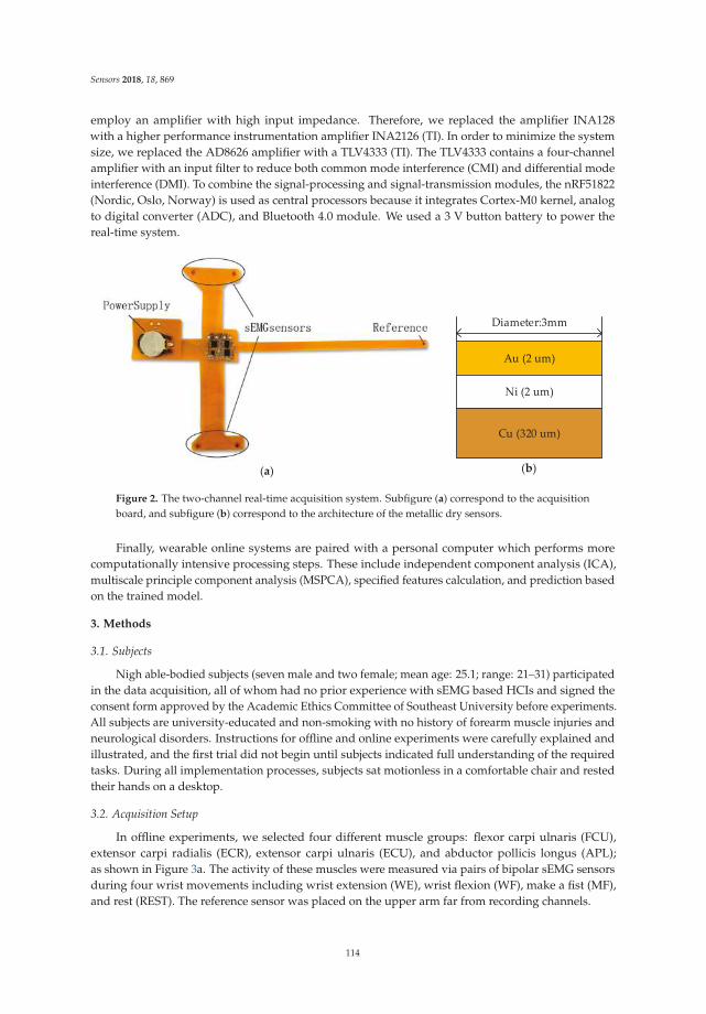
Sensors 2018, 18, 869

employ an amplifier with high input impedance. Therefore, we replaced the amplifier INA128with a higher performance instrumentation amplifier INA2126 (TI). In order to minimize the systemsize, we replaced the AD8626 amplifier with a TLV4333 (TI). The TLV4333 contains a four-channelamplifier with an input filter to reduce both common mode interference (CMI) and differential modeinterference (DMI). To combine the signal-processing and signal-transmission modules, the nRF51822(Nordic, Oslo, Norway) is used as central processors because it integrates Cortex-M0 kernel, analogto digital converter (ADC), and Bluetooth 4.0 module. We used a 3 V button battery to power thereal-time system.

(a)

Au (2 um)

Ni (2 um)

Cu (320 um)

Diameter:3mm

(b)

Figure 2. The two-channel real-time acquisition system. Subfigure (a) correspond to the acquisitionboard, and subfigure (b) correspond to the architecture of the metallic dry sensors.

Finally, wearable online systems are paired with a personal computer which performs morecomputationally intensive processing steps. These include independent component analysis (ICA),multiscale principle component analysis (MSPCA), specified features calculation, and prediction basedon the trained model.

3. Methods

3.1. Subjects

Nigh able-bodied subjects (seven male and two female; mean age: 25.1; range: 21–31) participatedin the data acquisition, all of whom had no prior experience with sEMG based HCIs and signed theconsent form approved by the Academic Ethics Committee of Southeast University before experiments.All subjects are university-educated and non-smoking with no history of forearm muscle injuries andneurological disorders. Instructions for offline and online experiments were carefully explained andillustrated, and the first trial did not begin until subjects indicated full understanding of the requiredtasks. During all implementation processes, subjects sat motionless in a comfortable chair and restedtheir hands on a desktop.

3.2. Acquisition Setup

In offline experiments, we selected four different muscle groups: flexor carpi ulnaris (FCU),extensor carpi radialis (ECR), extensor carpi ulnaris (ECU), and abductor pollicis longus (APL);as shown in Figure 3a. The activity of these muscles were measured via pairs of bipolar sEMG sensorsduring four wrist movements including wrist extension (WE), wrist flexion (WF), make a fist (MF),and rest (REST). The reference sensor was placed on the upper arm far from recording channels.

114

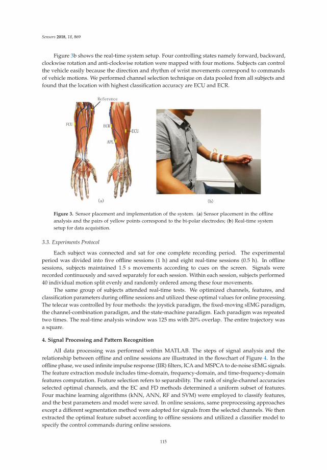
Sensors 2018, 18, 869

Figure 3b shows the real-time system setup. Four controlling states namely forward, backward,clockwise rotation and anti-clockwise rotation were mapped with four motions. Subjects can controlthe vehicle easily because the direction and rhythm of wrist movements correspond to commandsof vehicle motions. We performed channel selection technique on data pooled from all subjects andfound that the location with highest classification accuracy are ECU and ECR.

Figure 3. Sensor placement and implementation of the system. (a) Sensor placement in the offlineanalysis and the pairs of yellow points correspond to the bi-polar electrodes; (b) Real-time systemsetup for data acquisition.

3.3. Experiments Protocol

Each subject was connected and sat for one complete recording period. The experimentalperiod was divided into five offline sessions (1 h) and eight real-time sessions (0.5 h). In offlinesessions, subjects maintained 1.5 s movements according to cues on the screen. Signals wererecorded continuously and saved separately for each session. Within each session, subjects performed40 individual motion split evenly and randomly ordered among these four movements.

The same group of subjects attended real-time tests. We optimized channels, features, andclassification parameters during offline sessions and utilized these optimal values for online processing.The telecar was controlled by four methods: the joystick paradigm, the fixed-moving sEMG paradigm,the channel-combination paradigm, and the state-machine paradigm. Each paradigm was repeatedtwo times. The real-time analysis window was 125 ms with 20% overlap. The entire trajectory wasa square.

4. Signal Processing and Pattern Recognition

All data processing was performed within MATLAB. The steps of signal analysis and therelationship between offline and online sessions are illustrated in the flowchart of Figure 4. In theoffline phase, we used infinite impulse response (IIR) filters, ICA and MSPCA to de-noise sEMG signals.The feature extraction module includes time-domain, frequency-domain, and time-frequency-domainfeatures computation. Feature selection refers to separability. The rank of single-channel accuraciesselected optimal channels, and the EC and FD methods determined a uniform subset of features.Four machine learning algorithms (kNN, ANN, RF and SVM) were employed to classify features,and the best parameters and model were saved. In online sessions, same preprocessing approachesexcept a different segmentation method were adopted for signals from the selected channels. We thenextracted the optimal feature subset according to offline sessions and utilized a classifier model tospecify the control commands during online sessions.

115

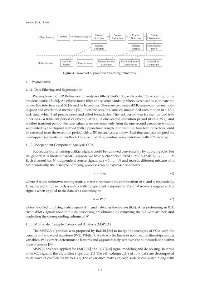
Sensors 2018, 18, 869

Figure 4. Flowchart of proposed processing framework.

4.1. Preprocessing

4.1.1. Data Filtering and Segmentation

We employed an IIR Butterworth bandpass filter (10–450 Hz, with order 16) according to theprevious works [54,56]. An elliptic notch filter and several bandstop filters were used to eliminate thepower line interference at 50 Hz and its harmonics. There are two main sEMG segmentation methods:disjoint and overlapped methods [57]. In offline sessions, subjects maintained each motion in a 1.5-stask time, which had precise onset and offset boundaries. The task period was further divided into3 periods—a transient period of onset (0–0.25 s); a one-second execution period (0.25–1.25 s); andanother transient period. Feature values were extracted only from the one-second execution windowsegmented by the disjoint method with a predefined length. For example, four feature vectors couldbe extracted from the execution period with a 250 ms analysis window. Real-time analysis adopted theoverlapped segmentation method. The size of sliding window was predefined with 20% overlap.

4.1.2. Independent Component Analysis (ICA)

Subsequently, remaining artifact signals could be removed conveniently by applying ICA. Forthe general ICA model of sEMG, suppose we have N channels filtered sEMG signals xi, i = 1, . . . , N.Each channel has N independent source signals si, i = 1, . . . , N and records different mixture of si.Mathematically, the principle of mixing processes can be expressed as follows:

x = A·s, (1)

where A is the unknown mixing matrix, x and s represent the combination of xi and si respectively.Then, the algorithm extracts a matrix with independent components (ICs) that recovers original sEMGsignals when applied to the data set x according to:

u = W·x, (2)

where W called unmixing matrix equals A−1, and u denotes the sources (ICs). After performing an ICA,clean sEMG signals used in future processing are obtained by removing the ICs with artifacts andneglecting the corresponding column of W.

4.1.3. Multiscale Principle Component Analysis (MSPCA)

The MSPCA algorithm was proposed by Bakshi [58] to merge the strengths of PCA with thebenefits of the wavelet transform (WT). While PCA extracts the linear or nonlinear relationships amongvariables, WT extracts deterministic features and approximately removes the autocorrelation withinmeasurements [59].

MSPCA has been applied for EMG [36] and ECG [60] signal modeling and de-noising. In termsof sEMG signals, the algorithm steps are: (1) The j-th column xj(t) of raw data are decomposedto its wavelet coefficients by WT. (2) The covariance matrix of each scale is computed along with

116

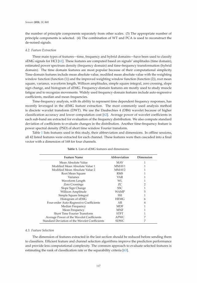
Sensors 2018, 18, 869

the number of principle components separately from other scales. (3) The appropriate number ofprinciple components is selected. (4) The combination of WT and PCA is used to reconstruct thede-noised signals.

4.2. Feature Extraction

Three main types of features—time, frequency and hybrid domains—have been used to classifysEMG signals for HCI [61]. These features are computed based on signals’ amplitudes (time domain),estimated power spectrum density (frequency domain) and time-frequency transformation (hybriddomain). The time domain features are most popular because of their computational simplicity.Time-domain features include mean absolute value, modified mean absolute value with the weightingwindow function (function (1)) and the improved weighting window function (function (2)), root meansquare, variance, waveform length, Willison amplitudes, simple square integral, zero crossing, slopesign change, and histogram of sEMG. Frequency-domain features are mostly used to study musclefatigue and to recognize movements. Widely used frequency-domain features include auto-regressivecoefficients, median and mean frequencies.

Time-frequency analysis, with its ability to represent time dependent frequency responses, hasrecently leveraged in the sEMG feature extraction. The most commonly used analysis methodis discrete wavelet transform (DWT). We use the Daubechies 4 (DB4) wavelet because of higherclassification accuracy and lower computation cost [62]. Average power of wavelet coefficients ineach sub-band are extracted for evaluation of the frequency distribution. We also compute standarddeviation of coefficients to evaluate changes in the distribution. Another time-frequency feature ispower spectral density (PSD) of short time window Fourier transform.

Table 1 lists features used in this study, their abbreviation and dimensions. In offline sessions,all 42 listed features were extracted for each channel. These features were then cascaded into a finalvector with a dimension of 168 for four channels.

Table 1. List of sEMG features and dimensions.

Feature Name Abbreviation Dimension

Mean Absolute Value MAV 1Modified Mean Absolute Value 1 MMAV1 1Modified Mean Absolute Value 2 MMAV2 1

Root Mean Square RMS 1Variance VAR 1

Waveform Length WL 1Zero Crossings ZC 2

Slope Sign Change SSC 1Willison Amplitude WAMP 5

Simple Square Integral SSI 1Histogram of sEMG HEMG 6

Four-order Auto-Regressive Coefficients AR 4Median Frequency MDF 1Mean Frequency MNF 1

Short Time Fourier Transform STFT 1Average Power of the Wavelet Coefficients APWC 7

Standard Deviation of the Wavelet Coefficients SDWC 7

4.3. Feature Selection

The dimension of features extracted in the last section should be reduced before sending themto classifiers. Efficient feature and channel selection algorithms improve the prediction performanceand provide less computational complexity. The common approach to evaluate selected features isestimating the rank of classification rate or the separability criteria [63].

117

Sensors 2018, 18, 869

Here, the optimal-feature selection combined the rank of separability values (SV) of each featurewith classification rates by SVM. First, we obtained a feature subset with the highest accuracy forindividual channel. The mean number of optimal feature subsets across all channels and subjectsrepresented the size of features in real-time algorithms. Next step was to confirm the detailed commonfeatures. We calculated the summation of each feature’s SV via EC and FD methods. We then usedthe RFE method to compute and rank the frequency each feature was contained in optimal subsets.The selected features were determined by specific criteria according to these different methods. Ideally,different algorithms should obtain almost same optimal feature subsets.

4.3.1. Entropy Criterion Based Feature Selection (EC)

A modified entropy based method is used to calculate separability values. The variance of featuresamong different classes can provide classification information, and the entropy of features’ variance isa measurement of uncertainty. When the variance of different classes is close, it means that the specificclass has little classification information and vice versa. Therefore, the entropy of variance measuresseparability of each feature. The definition is as follows:

Ji = −n

∑k=1

Vik · ln(Vi

k), (3)

where Ji denotes SV of the i-th feature, and Vik denotes normalized variance of the i-th feature for

the k-th class (totally n class). Within this method, smaller Ji corresponds to the feature with largervariance entropy.

4.3.2. Fisher Discrimination Based Feature Selection (FD)

The ratio of between-class and within-class distance could evaluate the extracted features’separability numerically. The principle of this method is similar with the Fisher linear discriminantanalysis (LDA) algorithm [64]. The SV is calculated by:

Ji = D2(ai, bi)/(D2(ai, ai) + D2(bi, bi)), (4)

where ai and bi denote the i-th feature in class a and b respectively, and the function D2(a,b) is themean Euclidean distance between all combination of different trials of two groups. The separabilityimproves when the ratio increases. In multi-class (totally n class) separability analysis, we separate theproblem into n two-class problems according to one-versus-all strategy [65]. The average ratio of thesetwo-class problems is computed as the multi-class SV for each feature.

4.3.3. Recursive Feature Elimination (RFE)

Compared with the mentioned methods offering the numerical evaluation of features, the RFEalgorithm based on SVM outputs a list of ranked features. In detail, the RFE algorithm mainly containsfollowing steps [66]. (1) Features and class labels are combined. (2) Training the model of SVM.(3) Computing the weight vector and rank criteria. (4) The feature with the smallest rank criteria iseliminated. (5) Steps (2)–(4) are repeated until only one feature is left. Finally, the algorithm outputsthe feature rank list. The rank criteria is the squared coefficients w2 [67]. Importance of a feature isdetermined by the loss of the margin between classification boundaries when the feature is removed.The rank criteria is defined as:

Ji = mini

∣∣∣w − w(−i)∣∣∣, (5)

where w is the inverse of margins which means w = ‖w‖2, and w(−i) represents the w without the i-thfeature at this SVM iteration.

118

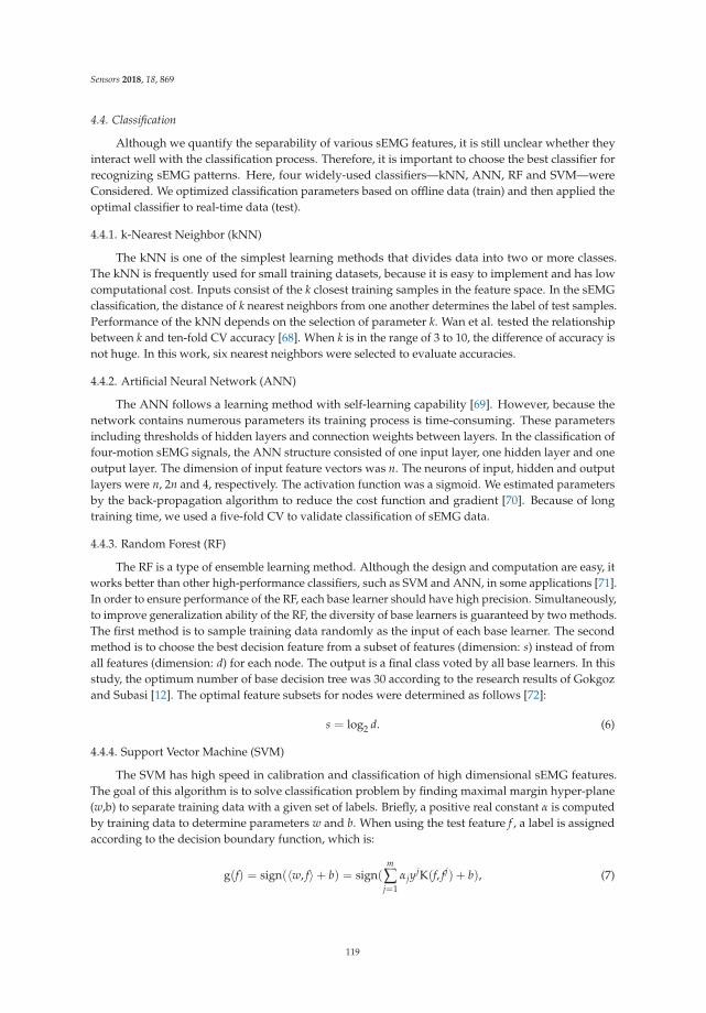
Sensors 2018, 18, 869

4.4. Classification

Although we quantify the separability of various sEMG features, it is still unclear whether theyinteract well with the classification process. Therefore, it is important to choose the best classifier forrecognizing sEMG patterns. Here, four widely-used classifiers—kNN, ANN, RF and SVM—wereConsidered. We optimized classification parameters based on offline data (train) and then applied theoptimal classifier to real-time data (test).

4.4.1. k-Nearest Neighbor (kNN)

The kNN is one of the simplest learning methods that divides data into two or more classes.The kNN is frequently used for small training datasets, because it is easy to implement and has lowcomputational cost. Inputs consist of the k closest training samples in the feature space. In the sEMGclassification, the distance of k nearest neighbors from one another determines the label of test samples.Performance of the kNN depends on the selection of parameter k. Wan et al. tested the relationshipbetween k and ten-fold CV accuracy [68]. When k is in the range of 3 to 10, the difference of accuracy isnot huge. In this work, six nearest neighbors were selected to evaluate accuracies.

4.4.2. Artificial Neural Network (ANN)

The ANN follows a learning method with self-learning capability [69]. However, because thenetwork contains numerous parameters its training process is time-consuming. These parametersincluding thresholds of hidden layers and connection weights between layers. In the classification offour-motion sEMG signals, the ANN structure consisted of one input layer, one hidden layer and oneoutput layer. The dimension of input feature vectors was n. The neurons of input, hidden and outputlayers were n, 2n and 4, respectively. The activation function was a sigmoid. We estimated parametersby the back-propagation algorithm to reduce the cost function and gradient [70]. Because of longtraining time, we used a five-fold CV to validate classification of sEMG data.

4.4.3. Random Forest (RF)

The RF is a type of ensemble learning method. Although the design and computation are easy, itworks better than other high-performance classifiers, such as SVM and ANN, in some applications [71].In order to ensure performance of the RF, each base learner should have high precision. Simultaneously,to improve generalization ability of the RF, the diversity of base learners is guaranteed by two methods.The first method is to sample training data randomly as the input of each base learner. The secondmethod is to choose the best decision feature from a subset of features (dimension: s) instead of fromall features (dimension: d) for each node. The output is a final class voted by all base learners. In thisstudy, the optimum number of base decision tree was 30 according to the research results of Gokgozand Subasi [12]. The optimal feature subsets for nodes were determined as follows [72]:

s = log2 d. (6)

4.4.4. Support Vector Machine (SVM)

The SVM has high speed in calibration and classification of high dimensional sEMG features.The goal of this algorithm is to solve classification problem by finding maximal margin hyper-plane(w,b) to separate training data with a given set of labels. Briefly, a positive real constant α is computedby training data to determine parameters w and b. When using the test feature f , a label is assignedaccording to the decision boundary function, which is:

g(f) = sign(〈w, f〉+ b) = sign(m

∑j=1

αjyjK(f, fj) + b), (7)

119

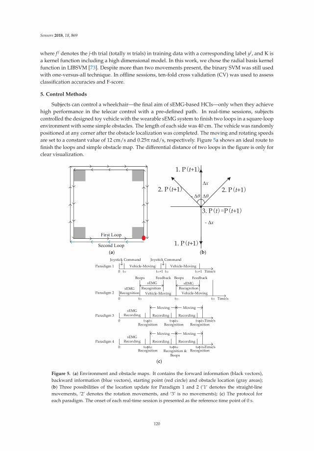
Sensors 2018, 18, 869

where f j denotes the j-th trial (totally m trials) in training data with a corresponding label yj, and K isa kernel function including a high dimensional model. In this work, we chose the radial basis kernelfunction in LIBSVM [73]. Despite more than two movements present, the binary SVM was still usedwith one-versus-all technique. In offline sessions, ten-fold cross validation (CV) was used to assessclassification accuracies and F-score.

5. Control Methods

Subjects can control a wheelchair—the final aim of sEMG-based HCIs—only when they achievehigh performance in the telecar control with a pre-defined path. In real-time sessions, subjectscontrolled the designed toy vehicle with the wearable sEMG system to finish two loops in a square-loopenvironment with some simple obstacles. The length of each side was 40 cm. The vehicle was randomlypositioned at any corner after the obstacle localization was completed. The moving and rotating speedsare set to a constant value of 12 cm/s and 0.25π rad/s, respectively. Figure 5a shows an ideal route tofinish the loops and simple obstacle map. The differential distance of two loops in the figure is only forclear visualization.

1. P t+1

1. P t+1

x

x

2. P t+1 2. P t+1

3. P t P t+1

(a) (b)

0 t11

Paradigm 1

t11+1 t12 t12+1

Joystick Command

Vehicle-Moving

Joystick Command

Vehicle-Moving

Paradigm 2sEMG

Recognition Vehicle-Moving

Beeps

Recognition

Feedback

sEMG

Beeps

sEMG

Recognition

Feedback

Vehicle-Moving

0 t21 t22 t23

Time/s

Time/s

Paradigm 3

sEMG Recording

Recognition

Recording

Time/s

Recording

0 t31 t32 t33 t34 t35

Paradigm 4sEMG

Recording Recording Recording

Time/s0 t41 t42 t43 t44 t45

Recognitiont36

Moving Moving

Recognition

Recognition Recognition &Beeps

t46

Recognition

Moving Moving

(c)

Figure 5. (a) Environment and obstacle maps. It contains the forward information (black vectors),backward information (blue vectors), starting point (red circle) and obstacle location (gray areas);(b) Three possibilities of the location update for Paradigm 1 and 2 (‘1’ denotes the straight-linemovements, ‘2’ denotes the rotation movements, and ‘3’ is no movements); (c) The protocol foreach paradigm. The onset of each real-time session is presented as the reference time point of 0 s.

120

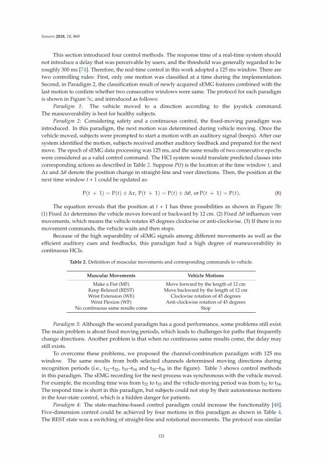
Sensors 2018, 18, 869

This section introduced four control methods. The response time of a real-time system shouldnot introduce a delay that was perceivable by users, and the threshold was generally regarded to beroughly 300 ms [74]. Therefore, the real-time control in this work adopted a 125 ms window. There aretwo controlling rules: First, only one motion was classified at a time during the implementation.Second, in Paradigm 2, the classification result of newly acquired sEMG features combined with thelast motion to confirm whether two consecutive windows were same. The protocol for each paradigmis shown in Figure 5c, and introduced as follows:

Paradigm 1: The vehicle moved to a direction according to the joystick command.The maneuverability is best for healthy subjects.

Paradigm 2: Considering safety and a continuous control, the fixed-moving paradigm wasintroduced. In this paradigm, the next motion was determined during vehicle moving. Once thevehicle moved, subjects were prompted to start a motion with an auditory signal (beeps). After oursystem identified the motion, subjects received another auditory feedback and prepared for the nextmove. The epoch of sEMG data processing was 125 ms, and the same results of two consecutive epochswere considered as a valid control command. The HCI system would translate predicted classes intocorresponding actions as described in Table 2. Suppose P(t) is the location at the time window t, and∆x and ∆θ denote the position change in straight-line and veer directions. Then, the position at thenext time window t + 1 could be updated as:

P(t + 1) = P(t)± ∆x, P(t + 1) = P(t)± ∆θ, or P(t + 1) = P(t). (8)

The equation reveals that the position at t + 1 has three possibilities as shown in Figure 5b:(1) Fixed ∆x determines the vehicle moves forward or backward by 12 cm. (2) Fixed ∆θ influences veermovements, which means the vehicle rotates 45 degrees clockwise or anti-clockwise. (3) If there is nomovement commands, the vehicle waits and then stops.

Because of the high separability of sEMG signals among different movements as well as theefficient auditory cues and feedbacks, this paradigm had a high degree of maneuverability incontinuous HCIs.

Table 2. Definition of muscular movements and corresponding commands to vehicle.

Muscular Movements Vehicle Motions

Make a Fist (MF) Move forward by the length of 12 cmKeep Relaxed (REST) Move backward by the length of 12 cmWrist Extension (WE) Clockwise rotation of 45 degrees

Wrist Flexion (WF) Anti-clockwise rotation of 45 degreesNo continuous same results come Stop

Paradigm 3: Although the second paradigm has a good performance, some problems still exist.The main problem is about fixed moving periods, which leads to challenges for paths that frequentlychange directions. Another problem is that when no continuous same results come, the delay maystill exists.

To overcome these problems, we proposed the channel-combination paradigm with 125 mswindow. The same results from both selected channels determined moving directions duringrecognition periods (i.e., t31–t32, t33–t34 and t35–t36 in the figure). Table 3 shows control methodsin this paradigm. The sEMG recording for the next process was synchronous with the vehicle moved.For example, the recording time was from t32 to t33 and the vehicle-moving period was from t32 to t34.The respond time is short in this paradigm, but subjects could not stop by their autonomous motionsin the four-state control, which is a hidden danger for patients.

Paradigm 4: The state-machine-based control paradigm could increase the functionality [48].Five-dimension control could be achieved by four motions in this paradigm as shown in Table 4.The REST state was a switching of straight-line and rotational movements. The protocol was similar

121

Sensors 2018, 18, 869

with Paradigm 3 in Figure 5c. The initial state was straight-line movements, and the detailed controlmethod was as following. Recognition results from t41–t42 determined moving states in t42–t44. Uponthe REST state appeared (e.g., the period of t43–t44), an auditory beeps was offered and the mode wasswitched to rotational movements. Consequently, another REST state set back the mode to straight-linestate. A critical control rule was the mode could not be changed unless at least one motion wasimplemented. Subjects can stop control by keeping fisting.

Table 3. Definition of muscular movements and control method in Paradigm 3 and 4.

Muscular Movements Control Method Vehicle Motions

Make a Fist (MF) Ch1 = Ch2 = 1 ForwardKeep Relaxed (REST) Ch1 = Ch2 = 2 BackwardWrist Extension (WE) Ch1 = Ch2 = 3 Clockwise rotation

Wrist Flexion (WF) Ch1 = Ch2 = 4 Anti-clockwise rotationOthers Ch1 �= Ch2 Stop

Table 4. Definition of muscular movements and control method in Paradigm 5 and 6.

Muscular Movements Vehicle Motions

Keep Relaxed (REST) Switching: on/offWrist Flexion (WF) On: Forward Off: Anti-clockwise rotation

Wrist Extension (WE) On: Backward Off: Clockwise rotationMake a Fist (MF) Stop

6. Results

Our objective is to choose and use effective features for the sEMG-controlled vehicle with wearableHCI designed by our group. We present four steps: first, we validate the feasibility and performanceof our proposed hardware and filters. Second, the rank of classification accuracy picks two channels.Thirdly, optimal feature subsets and multi-class recognition rates are computed by the proposed featureselection algorithms, and compared with the RFE method. Finally, we generalize findings throughcomparing different control paradigms, and investigate whether the selected common channels andfeatures are applicable to online sessions.

6.1. Acquisition System Testing

Tests of this part are to verify the feasibility of acquisition systems and preprocessing methods.The results show that real-time high-quality signals can be transmitted to computers and saved withinthe Bluetooth communication distance.

6.1.1. Hardware Evaluation

Signal amplifiers and filters are the main components in acquisition systems. Two stages ofamplifiers were used to avoid effects on the signals’ bandwidth when the gain of one stage amplifierwas too large. The first stage amplifier has a large input impedance, and the gain is 51. The secondstage is an inverting amplifier with high gain (−35.7), gain bandwidth product (GBP) and CMRR.Therefore, the total gain for amplification of raw sEMG signals is −1821 as shown in Figure 6a.

The acquisition systems contain a low-pass filter of 450 Hz, a high-pass filter of 10 Hz and a notchfilter of 50 Hz. We validated designs of filters and circuit components in the FilterPro (TI) insteadof via manual derivation process. The low-pass and high-pass filters are four-order and two-orderButterworth structure with the Sallen-Key topology, respectively. In addition, a 50 Hz notch filter isintegrated in the UAF42.

Frequency responses of filters were measured by applying a 1 Vpp sinusoidal signallogarithmically generated by a function generator. Figure 6 depicts the amplitude-versus-frequency

122

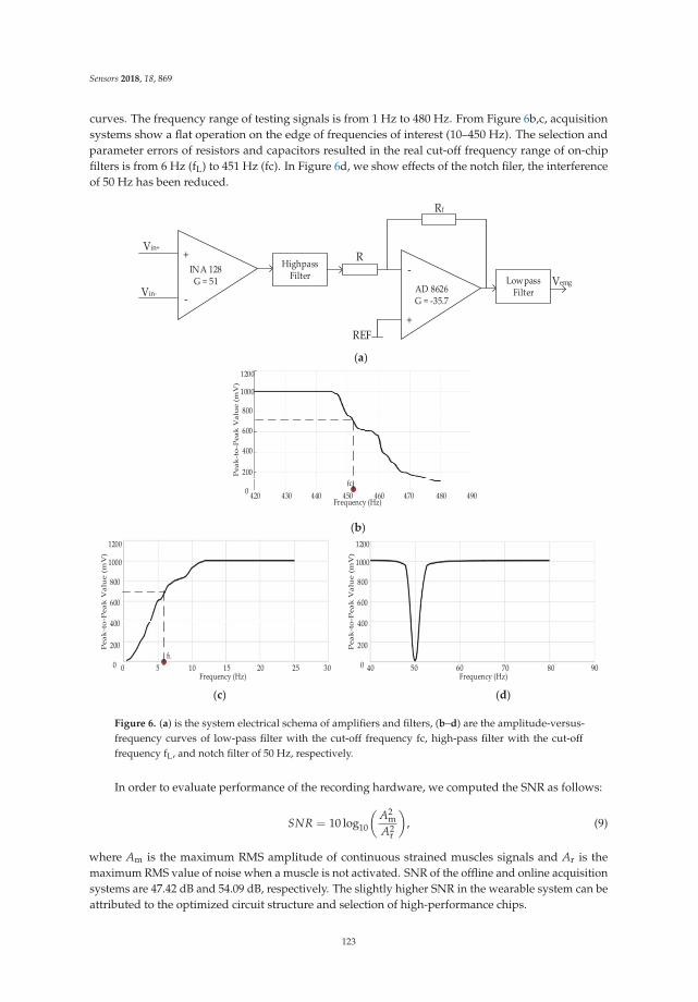
Sensors 2018, 18, 869

curves. The frequency range of testing signals is from 1 Hz to 480 Hz. From Figure 6b,c, acquisitionsystems show a flat operation on the edge of frequencies of interest (10–450 Hz). The selection andparameter errors of resistors and capacitors resulted in the real cut-off frequency range of on-chipfilters is from 6 Hz (fL) to 451 Hz (fc). In Figure 6d, we show effects of the notch filer, the interferenceof 50 Hz has been reduced.

INA 128G = 51

Vin+

Vin-

HighpassFilter

REF

LowpassFilter

Vemg

R

Rf

AD 8626G = -35.7

+

-

-

+

(a)

1200

1000

800

600

400

200

0420 430 440 450 460 470 480 490

Frequency (Hz)

Pea

k-t

o-P

ea

k V

alu

e (

mV

)

fc

(b)

1200

1000

800

600

400

200

0 0 5 10 15 20 25 30Frequency (Hz)

Pea

k-t

o-P

ea

k V

alu

e (

mV

)

fL

1200

1000

800

600

400

200

0 40 50 60 70 80 90Frequency (Hz)

Pea

k-t

o-P

ea

k V

alu

e (

mV

)

(c) (d)

Figure 6. (a) is the system electrical schema of amplifiers and filters, (b–d) are the amplitude-versus-frequency curves of low-pass filter with the cut-off frequency fc, high-pass filter with the cut-offfrequency fL, and notch filter of 50 Hz, respectively.

In order to evaluate performance of the recording hardware, we computed the SNR as follows:

SNR = 10 log10

(A2

mA2

r

), (9)

where Am is the maximum RMS amplitude of continuous strained muscles signals and Ar is themaximum RMS value of noise when a muscle is not activated. SNR of the offline and online acquisitionsystems are 47.42 dB and 54.09 dB, respectively. The slightly higher SNR in the wearable system can beattributed to the optimized circuit structure and selection of high-performance chips.

123

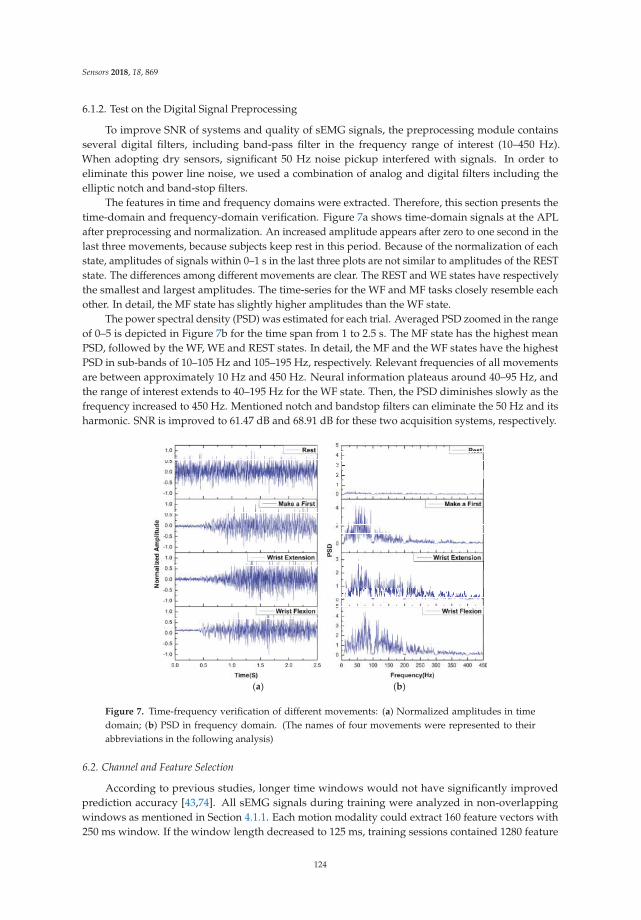
Sensors 2018, 18, 869

6.1.2. Test on the Digital Signal Preprocessing

To improve SNR of systems and quality of sEMG signals, the preprocessing module containsseveral digital filters, including band-pass filter in the frequency range of interest (10–450 Hz).When adopting dry sensors, significant 50 Hz noise pickup interfered with signals. In order toeliminate this power line noise, we used a combination of analog and digital filters including theelliptic notch and band-stop filters.

The features in time and frequency domains were extracted. Therefore, this section presents thetime-domain and frequency-domain verification. Figure 7a shows time-domain signals at the APLafter preprocessing and normalization. An increased amplitude appears after zero to one second in thelast three movements, because subjects keep rest in this period. Because of the normalization of eachstate, amplitudes of signals within 0–1 s in the last three plots are not similar to amplitudes of the RESTstate. The differences among different movements are clear. The REST and WE states have respectivelythe smallest and largest amplitudes. The time-series for the WF and MF tasks closely resemble eachother. In detail, the MF state has slightly higher amplitudes than the WF state.

The power spectral density (PSD) was estimated for each trial. Averaged PSD zoomed in the rangeof 0–5 is depicted in Figure 7b for the time span from 1 to 2.5 s. The MF state has the highest meanPSD, followed by the WF, WE and REST states. In detail, the MF and the WF states have the highestPSD in sub-bands of 10–105 Hz and 105–195 Hz, respectively. Relevant frequencies of all movementsare between approximately 10 Hz and 450 Hz. Neural information plateaus around 40–95 Hz, andthe range of interest extends to 40–195 Hz for the WF state. Then, the PSD diminishes slowly as thefrequency increased to 450 Hz. Mentioned notch and bandstop filters can eliminate the 50 Hz and itsharmonic. SNR is improved to 61.47 dB and 68.91 dB for these two acquisition systems, respectively.

(a) (b)

Figure 7. Time-frequency verification of different movements: (a) Normalized amplitudes in timedomain; (b) PSD in frequency domain. (The names of four movements were represented to theirabbreviations in the following analysis)

6.2. Channel and Feature Selection

According to previous studies, longer time windows would not have significantly improvedprediction accuracy [43,74]. All sEMG signals during training were analyzed in non-overlappingwindows as mentioned in Section 4.1.1. Each motion modality could extract 160 feature vectors with250 ms window. If the window length decreased to 125 ms, training sessions contained 1280 feature

124

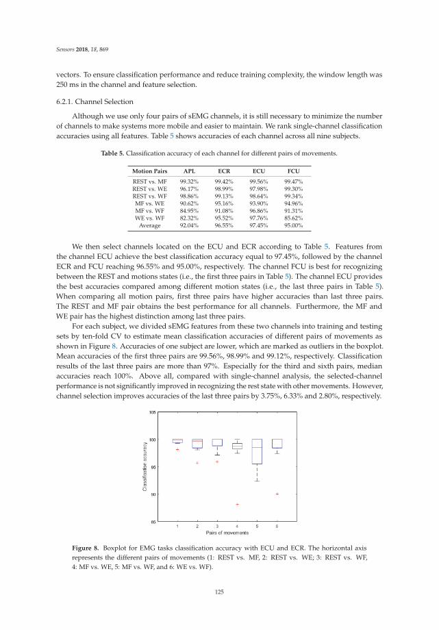
Sensors 2018, 18, 869

vectors. To ensure classification performance and reduce training complexity, the window length was250 ms in the channel and feature selection.

6.2.1. Channel Selection

Although we use only four pairs of sEMG channels, it is still necessary to minimize the numberof channels to make systems more mobile and easier to maintain. We rank single-channel classificationaccuracies using all features. Table 5 shows accuracies of each channel across all nine subjects.

Table 5. Classification accuracy of each channel for different pairs of movements.

Motion Pairs APL ECR ECU FCU

REST vs. MF 99.32% 99.42% 99.56% 99.47%REST vs. WE 96.17% 98.99% 97.98% 99.30%REST vs. WF 98.86% 99.13% 98.64% 99.34%MF vs. WE 90.62% 95.16% 93.90% 94.96%MF vs. WF 84.95% 91.08% 96.86% 91.31%WE vs. WF 82.32% 95.52% 97.76% 85.62%

Average 92.04% 96.55% 97.45% 95.00%

We then select channels located on the ECU and ECR according to Table 5. Features fromthe channel ECU achieve the best classification accuracy equal to 97.45%, followed by the channelECR and FCU reaching 96.55% and 95.00%, respectively. The channel FCU is best for recognizingbetween the REST and motions states (i.e., the first three pairs in Table 5). The channel ECU providesthe best accuracies compared among different motion states (i.e., the last three pairs in Table 5).When comparing all motion pairs, first three pairs have higher accuracies than last three pairs.The REST and MF pair obtains the best performance for all channels. Furthermore, the MF andWE pair has the highest distinction among last three pairs.

For each subject, we divided sEMG features from these two channels into training and testingsets by ten-fold CV to estimate mean classification accuracies of different pairs of movements asshown in Figure 8. Accuracies of one subject are lower, which are marked as outliers in the boxplot.Mean accuracies of the first three pairs are 99.56%, 98.99% and 99.12%, respectively. Classificationresults of the last three pairs are more than 97%. Especially for the third and sixth pairs, medianaccuracies reach 100%. Above all, compared with single-channel analysis, the selected-channelperformance is not significantly improved in recognizing the rest state with other movements. However,channel selection improves accuracies of the last three pairs by 3.75%, 6.33% and 2.80%, respectively.

Figure 8. Boxplot for EMG tasks classification accuracy with ECU and ECR. The horizontal axisrepresents the different pairs of movements (1: REST vs. MF, 2: REST vs. WE; 3: REST vs. WF,4: MF vs. WE, 5: MF vs. WF, and 6: WE vs. WF).

125

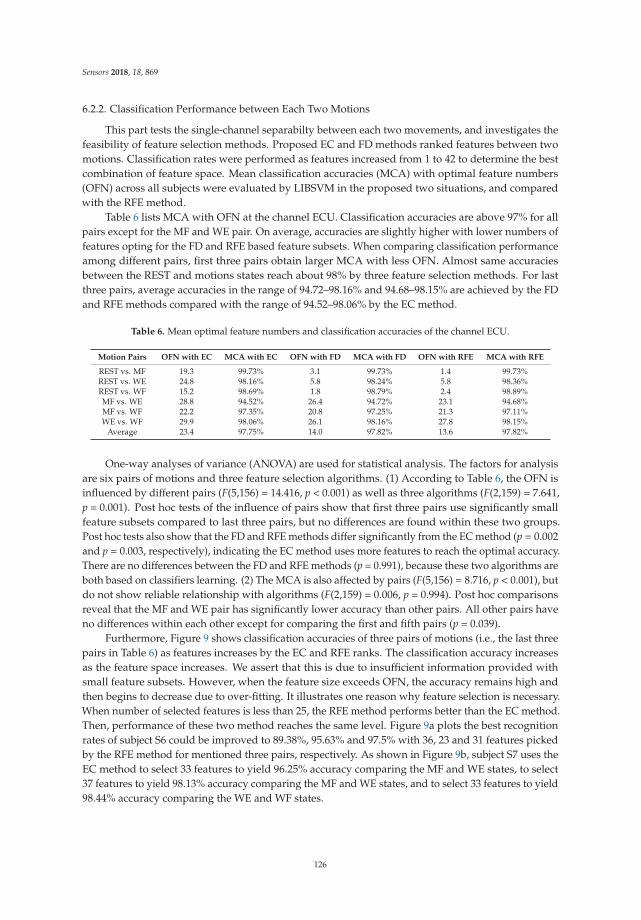
Sensors 2018, 18, 869

6.2.2. Classification Performance between Each Two Motions

This part tests the single-channel separabilty between each two movements, and investigates thefeasibility of feature selection methods. Proposed EC and FD methods ranked features between twomotions. Classification rates were performed as features increased from 1 to 42 to determine the bestcombination of feature space. Mean classification accuracies (MCA) with optimal feature numbers(OFN) across all subjects were evaluated by LIBSVM in the proposed two situations, and comparedwith the RFE method.

Table 6 lists MCA with OFN at the channel ECU. Classification accuracies are above 97% for allpairs except for the MF and WE pair. On average, accuracies are slightly higher with lower numbers offeatures opting for the FD and RFE based feature subsets. When comparing classification performanceamong different pairs, first three pairs obtain larger MCA with less OFN. Almost same accuraciesbetween the REST and motions states reach about 98% by three feature selection methods. For lastthree pairs, average accuracies in the range of 94.72–98.16% and 94.68–98.15% are achieved by the FDand RFE methods compared with the range of 94.52–98.06% by the EC method.

Table 6. Mean optimal feature numbers and classification accuracies of the channel ECU.

Motion Pairs OFN with EC MCA with EC OFN with FD MCA with FD OFN with RFE MCA with RFE

REST vs. MF 19.3 99.73% 3.1 99.73% 1.4 99.73%REST vs. WE 24.8 98.16% 5.8 98.24% 5.8 98.36%REST vs. WF 15.2 98.69% 1.8 98.79% 2.4 98.89%MF vs. WE 28.8 94.52% 26.4 94.72% 23.1 94.68%MF vs. WF 22.2 97.35% 20.8 97.25% 21.3 97.11%WE vs. WF 29.9 98.06% 26.1 98.16% 27.8 98.15%

Average 23.4 97.75% 14.0 97.82% 13.6 97.82%

One-way analyses of variance (ANOVA) are used for statistical analysis. The factors for analysisare six pairs of motions and three feature selection algorithms. (1) According to Table 6, the OFN isinfluenced by different pairs (F(5,156) = 14.416, p < 0.001) as well as three algorithms (F(2,159) = 7.641,p = 0.001). Post hoc tests of the influence of pairs show that first three pairs use significantly smallfeature subsets compared to last three pairs, but no differences are found within these two groups.Post hoc tests also show that the FD and RFE methods differ significantly from the EC method (p = 0.002and p = 0.003, respectively), indicating the EC method uses more features to reach the optimal accuracy.There are no differences between the FD and RFE methods (p = 0.991), because these two algorithms areboth based on classifiers learning. (2) The MCA is also affected by pairs (F(5,156) = 8.716, p < 0.001), butdo not show reliable relationship with algorithms (F(2,159) = 0.006, p = 0.994). Post hoc comparisonsreveal that the MF and WE pair has significantly lower accuracy than other pairs. All other pairs haveno differences within each other except for comparing the first and fifth pairs (p = 0.039).

Furthermore, Figure 9 shows classification accuracies of three pairs of motions (i.e., the last threepairs in Table 6) as features increases by the EC and RFE ranks. The classification accuracy increasesas the feature space increases. We assert that this is due to insufficient information provided withsmall feature subsets. However, when the feature size exceeds OFN, the accuracy remains high andthen begins to decrease due to over-fitting. It illustrates one reason why feature selection is necessary.When number of selected features is less than 25, the RFE method performs better than the EC method.Then, performance of these two method reaches the same level. Figure 9a plots the best recognitionrates of subject S6 could be improved to 89.38%, 95.63% and 97.5% with 36, 23 and 31 features pickedby the RFE method for mentioned three pairs, respectively. As shown in Figure 9b, subject S7 uses theEC method to select 33 features to yield 96.25% accuracy comparing the MF and WE states, to select37 features to yield 98.13% accuracy comparing the MF and WE states, and to select 33 features to yield98.44% accuracy comparing the WE and WF states.

126

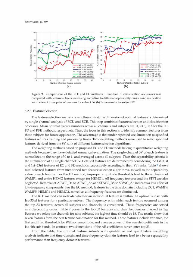
Sensors 2018, 18, 869

(a) (b)

Figure 9. Comparisons of the RFE and EC methods. Evolution of classification accuracies wascomputed with feature subsets increasing according to different separability ranks: (a) classificationaccuracies of three pairs of motions for subject S6; (b) Same results for subject S7.

6.2.3. Feature Selection

The feature selection analysis is as follows. First, the dimension of optimal features is determinedby single-channel analysis of ECU and ECR. This step combines feature selection and classificationprocesses. Mean optimal feature numbers across all channels and subjects are 31, 23.3, 32.8 for the EC,FD and RFE methods, respectively. Then, the focus in this section is to identify common features fromthese subjects for future application. The advantage is that under repeated use, limitation to specifiedfeatures reduces training and processing times. Two weighting methods were used to select specifiedfeatures derived from the SV rank of different feature selection algorithms.

The weighting methods based on proposed EC and FD methods belong to quantitative weightingmethods because they have detailed numerical evaluation. The single-channel SV of each feature isnormalized to the range of 0 to 1, and averaged across all subjects. Then the separability criteria isthe summation of all single-channel SV. Detailed features are determined by considering the 1st–31stand 1st–23rd features of EC and FD methods respectively according to their SV ranks. Table 7 showstotal selected features from mentioned two feature selection algorithms, as well as the separabilityvalue of each feature. For the FD method, improper amplitude thresholds lead to the exclusion ofWAMP1 and entire HEMG features except for HEMG1. All frequency features and the STFT are alsoneglected. Removal of APWC_D4 to APWC_A6 and SDWC_D5 to SDWC_A6 indicates a low effect oflow-frequency components. For the EC method, features in the time domain including ZC1, WAMP4,WAMP5, HEMG1 and HEMG2, as well as all frequency features are eliminated.

The RFE method can indicate whether an individual feature is within the optimal subset with1st–33rd features for a particular subject. The frequency with which each feature occurred amongthe top 33 features, across all subjects and channels, is considered. These frequencies are sortedin a descending order. Table 7 presents the top 33 features and their frequencies marked as T32.Because we select two channels for nine subjects, the highest time should be 18. The results show thatseven features form the best feature combination for this method. These features include variance, thefirst and third thresholds for Willison amplitude, and average power of the wavelet coefficients in the1st–4th sub-bands. In contrast, two dimensions of the AR coefficients never enter top 33.

From the table, the optimal feature subsets with qualitative and quantitative weightinganalysis indicate that time-domain and time-frequency-domain features lead to a better separabilityperformance than frequency-domain features.

127

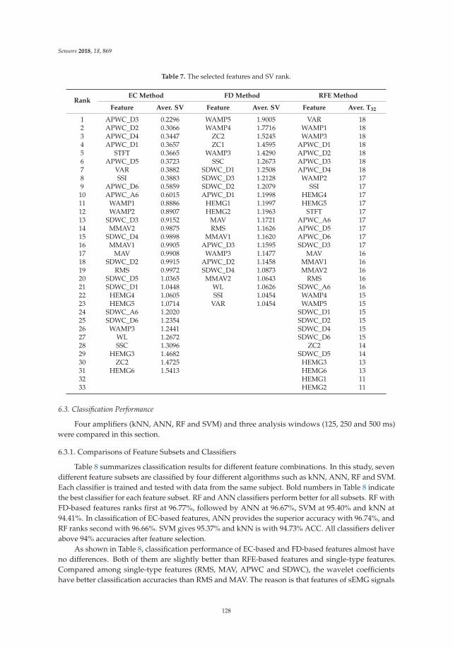
Sensors 2018, 18, 869

Table 7. The selected features and SV rank.

RankEC Method FD Method RFE Method

Feature Aver. SV Feature Aver. SV Feature Aver. T32

1 APWC_D3 0.2296 WAMP5 1.9005 VAR 182 APWC_D2 0.3066 WAMP4 1.7716 WAMP1 183 APWC_D4 0.3447 ZC2 1.5245 WAMP3 184 APWC_D1 0.3657 ZC1 1.4595 APWC_D1 185 STFT 0.3665 WAMP3 1.4290 APWC_D2 186 APWC_D5 0.3723 SSC 1.2673 APWC_D3 187 VAR 0.3882 SDWC_D1 1.2508 APWC_D4 188 SSI 0.3883 SDWC_D3 1.2128 WAMP2 179 APWC_D6 0.5859 SDWC_D2 1.2079 SSI 1710 APWC_A6 0.6015 APWC_D1 1.1998 HEMG4 1711 WAMP1 0.8886 HEMG1 1.1997 HEMG5 1712 WAMP2 0.8907 HEMG2 1.1963 STFT 1713 SDWC_D3 0.9152 MAV 1.1721 APWC_A6 1714 MMAV2 0.9875 RMS 1.1626 APWC_D5 1715 SDWC_D4 0.9898 MMAV1 1.1620 APWC_D6 1716 MMAV1 0.9905 APWC_D3 1.1595 SDWC_D3 1717 MAV 0.9908 WAMP3 1.1477 MAV 1618 SDWC_D2 0.9915 APWC_D2 1.1458 MMAV1 1619 RMS 0.9972 SDWC_D4 1.0873 MMAV2 1620 SDWC_D5 1.0365 MMAV2 1.0643 RMS 1621 SDWC_D1 1.0448 WL 1.0626 SDWC_A6 1622 HEMG4 1.0605 SSI 1.0454 WAMP4 1523 HEMG5 1.0714 VAR 1.0454 WAMP5 1524 SDWC_A6 1.2020 SDWC_D1 1525 SDWC_D6 1.2354 SDWC_D2 1526 WAMP3 1.2441 SDWC_D4 1527 WL 1.2672 SDWC_D6 1528 SSC 1.3096 ZC2 1429 HEMG3 1.4682 SDWC_D5 1430 ZC2 1.4725 HEMG3 1331 HEMG6 1.5413 HEMG6 1332 HEMG1 1133 HEMG2 11

6.3. Classification Performance

Four amplifiers (kNN, ANN, RF and SVM) and three analysis windows (125, 250 and 500 ms)were compared in this section.

6.3.1. Comparisons of Feature Subsets and Classifiers

Table 8 summarizes classification results for different feature combinations. In this study, sevendifferent feature subsets are classified by four different algorithms such as kNN, ANN, RF and SVM.Each classifier is trained and tested with data from the same subject. Bold numbers in Table 8 indicatethe best classifier for each feature subset. RF and ANN classifiers perform better for all subsets. RF withFD-based features ranks first at 96.77%, followed by ANN at 96.67%, SVM at 95.40% and kNN at94.41%. In classification of EC-based features, ANN provides the superior accuracy with 96.74%, andRF ranks second with 96.66%. SVM gives 95.37% and kNN is with 94.73% ACC. All classifiers deliverabove 94% accuracies after feature selection.

As shown in Table 8, classification performance of EC-based and FD-based features almost haveno differences. Both of them are slightly better than RFE-based features and single-type features.Compared among single-type features (RMS, MAV, APWC and SDWC), the wavelet coefficientshave better classification accuracies than RMS and MAV. The reason is that features of sEMG signals

128

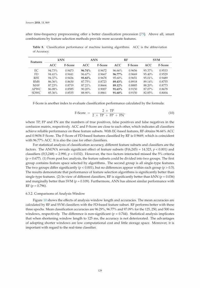
Sensors 2018, 18, 869

after time-frequency preprocessing offer a better classification precession [75]. Above all, smartcombinations by feature selection methods provide more accurate features.

Table 8. Classification performance of machine learning algorithms. ACC is the abbreviationof Accuracy.

FeatureskNN ANN RF SVM

ACC F-Score ACC F-Score ACC F-Score ACC F-Score

EC 94.73% 0.9473 96.74% 0.9672 96.66% 0.9656 95.37% 0.9533FD 94.41% 0.9441 96.67% 0.9667 96.77% 0.9669 95.40% 0.9529

RFE 94.37% 0.9436 95.82% 0.9678 95.60% 0.9651 95.01% 0.9489RMS 86.36% 0.8630 87.75% 0.8723 89.43% 0.8918 89.14% 0.8755MAV 87.23% 0.8719 87.21% 0.8664 89.12% 0.8885 88.20% 0.8773

APWC 86.08% 0.8585 90.20% 0.9007 91.63% 0.9150 87.07% 0.8678SDWC 85.36% 0.8535 88.90% 0.8861 91.60% 0.9150 82.85% 0.8004

F-Score is another index to evaluate classification performance calculated by the formula:

F-Score =2 × TP

2 × TP + FP + FN, (10)

where TP, FP and FN are the numbers of true positives, false positives and false negatives in theconfusion matrix, respectively. ACC and F-Score are close to each other, which indicates all classifiersachieve reliable performance on these feature subsets. With EC-based features, RF obtains 96.66% ACCand 0.9656 F-Score. The F-Score of FD-based features classified by RF is 0.9669, which is coincidentwith 96.77% ACC. It is also the case for other classifiers.

For statistical analysis of classification accuracy, different feature subsets and classifiers are thefactors. The ANOVA reveals significant effect of feature subsets (F(6,245) = 14.323, p < 0.001) andclassifiers (F(3,248) = 2.990, p = 0.032). However, the two factors interacted missed the 5% criteria(p = 0.677). (1) From post hoc analysis, the feature subsets could be divided into two groups. The firstgroup contains feature space selected by algorithms. The second group is all single-type features.The two groups differ significantly (p < 0.001), but no differences appear within each group (p > 0.5).The results demonstrate that performance of feature selection algorithms is significantly better thansingle-type features. (2) In view of different classifiers, RF is significantly better than kNN (p = 0.036)and marginally better than SVM (p = 0.109). Furthermore, ANN has almost similar performance withRF (p = 0.796).

6.3.2. Comparisons of Analysis Window

Figure 10 shows the effects of analysis window length and accuracies. The mean accuracies arecalculated by RF and SVM classifiers with the FD-based feature subset. RF performs better with thesethree epochs. Mean classification accuracies are 96.29%, 96.77% and 97.09% for the 125, 250, and 500 mswindows, respectively. The difference is non-significant (p = 0.744). Statistical analysis implicatesthat when shortening window length to 125 ms, the accuracy is not deteriorated. The advantagesof adopting shorter windows are low computational cost and little storage space. Moreover, it isimportant with regard to the real-time classifier.

129

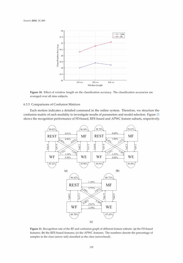
Sensors 2018, 18, 869

Figure 10. Effect of window length on the classification accuracy. The classification accuracies areaveraged over all nine subjects.

6.3.3. Comparisons of Confusion Matrices

Each motion indicates a detailed command in the online system. Therefore, we structure theconfusion matrix of each modality to investigate results of parameters and model selection. Figure 11shows the recognition performance of FD-based, RFE-based and APWC feature subsets, respectively.

(a) (b)

(c)

Figure 11. Recognition rate of the RF and confusion graph of different feature subsets: (a) the FD-basedfeatures; (b) the RFE-based features; (c) the APWC features. The numbers denote the percentage ofsamples in the class (arrow tail) classified as the class (arrowhead).

130

Sensors 2018, 18, 869

These features are extracted from 125 ms windows, and classified by RF. The FD method (REST:98.82%, MF: 96.10%, WE: 95.96% and WF: 95.32%) is slightly better than the RFE method (REST: 98.79%,MF: 95.67%, WE: 95.89% and WF: 94.93%). The feature selection process is helpful to classify all statescompared to single-type APWC features (REST: 96.42%, MF: 88.72%, WE: 87.43% and WF: 89.70%).The REST modality achieves the best recognition performance as sEMG amplitudes of keeping restand moving have large differences shown in Figure 7. Whereas, the MF, WE and WF modalities aremisclassified to others, especially for the MF and WE modalities. These observations are in line withthe results in previous sections. They indicate that assessment of multi-class recognition is feasiblewith proposed feature selection methods. Our proposed FD method can improve the predictionperformance and reduce the feature numbers compared with the conventional RFE method andsingle-type features.

6.4. Online Evaluation by Wearable EMG-based HCI

Each subject performs eight online sessions according to four separate paradigms. The selectedfeatures extracted from optimal channels and the trained RF model are opted for online sessions.Averaged recognition rates (RR) and travel time (TT) of each paradigm for all subjects are recorded andreferred to Table 9. In Paradigm 2, moving directions offer labels for classification. Therefore, the RRequals to classification accuracies. However, in Paradigm 3 and 4, subjects control the vehicle accordingto their thoughts. Here, the RR in Paradigm 3 denotes success rates of recognizing classification resultsof both channels are same. Since it is hard to define which motion is right in Paradigm 4, the RR is notpresented in Table 9 as a criterion.

Table 9. The recognition rate and travel time for different online paradigms.

SubjectParadigm 1 Paradigm 2 Paradigm 3 Paradigm 4

TT (s) RR TT (s) RR TT (s) RR TT (s) RR

S1 44.98 – 44.88 99.25% 47.21 96.88% 46.93 –S2 45.86 – 44.82 98.38% 50.31 89.61% 46.42 –S3 44.44 – 44.94 97.66% 45.07 98.03% 46.29 –S4 45.08 – 46.93 95.75% 48.87 95.77% 47.08 –S5 44.73 – 46.60 96.00% 47.10 92.50% 49.61 –S6 45.55 – 46.86 92.19% 51.43 84.45% 47.81 –S7 44.82 – 45.52 95.91% 48.87 96.09% 46.97 –S8 45.70 – 47.04 86.16% 52.03 85.08% 51.37 –S9 45.46 – 46.59 91.77% 50.67 88.54% 50.26 –

Mean 45.18 – 46.02 94.79% 49.06 91.77% 48.08 –

The results illustrate all subjects are able to complete these online paradigms with acceptableaccuracies and travel time. The TT in last three paradigms is close to the joystick paradigm (Paradigm 1).Averaged time of Paradigm 1 to finish the loops is 45.18 s. In the fixed-moving paradigm (Paradigm 2),subjects can accomplish two sessions within the mean time of 46.02 s with 95.01% RR. Paradigm 3and 4 increase the control time to 49.06 s and 48.08 s, respectively. The increment is achieved thatwhen two channels have different classification results in Paradigm 3, the vehicle stops and waits.Transience pauses also happen in mode switches during Paradigm 4. Although Paradigm 3 and 4 aremore sophisticated, these paradigms are closer to daily life. In Paradigm 2, only one command couldmake the vehicle move a fixed distance. However, in Paradigm 3 and 4, subjects decide each minormotion by their own ideas. Compared these two complex paradigms, subjects use less travel time inParadigm 4. The reason is that success rates are lower to ensure both channels have the same class forParadigm 3. S3 completes all sEMG-based sessions using the shortest time with the highest RR. On thecontrary, S8 performs the worst.

The rough relationship between the TT and RR in Paradigm 2 and 3 is that more TT uses, lessRR obtains. However, there are some special situations in detail. For example, the TT of S9 is similar

131

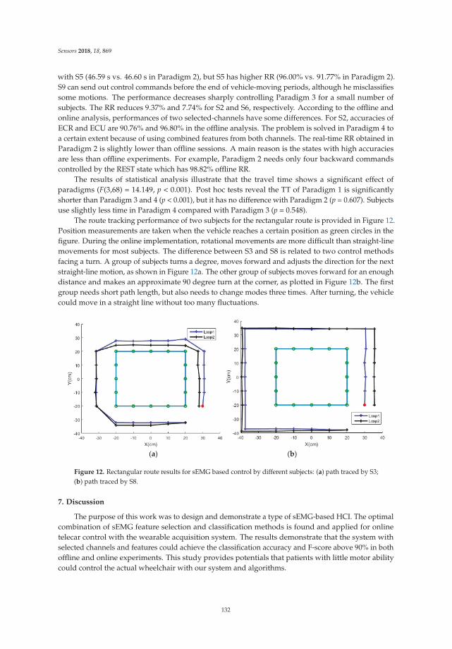
Sensors 2018, 18, 869

with S5 (46.59 s vs. 46.60 s in Paradigm 2), but S5 has higher RR (96.00% vs. 91.77% in Paradigm 2).S9 can send out control commands before the end of vehicle-moving periods, although he misclassifiessome motions. The performance decreases sharply controlling Paradigm 3 for a small number ofsubjects. The RR reduces 9.37% and 7.74% for S2 and S6, respectively. According to the offline andonline analysis, performances of two selected-channels have some differences. For S2, accuracies ofECR and ECU are 90.76% and 96.80% in the offline analysis. The problem is solved in Paradigm 4 toa certain extent because of using combined features from both channels. The real-time RR obtained inParadigm 2 is slightly lower than offline sessions. A main reason is the states with high accuraciesare less than offline experiments. For example, Paradigm 2 needs only four backward commandscontrolled by the REST state which has 98.82% offline RR.

The results of statistical analysis illustrate that the travel time shows a significant effect ofparadigms (F(3,68) = 14.149, p < 0.001). Post hoc tests reveal the TT of Paradigm 1 is significantlyshorter than Paradigm 3 and 4 (p < 0.001), but it has no difference with Paradigm 2 (p = 0.607). Subjectsuse slightly less time in Paradigm 4 compared with Paradigm 3 (p = 0.548).

The route tracking performance of two subjects for the rectangular route is provided in Figure 12.Position measurements are taken when the vehicle reaches a certain position as green circles in thefigure. During the online implementation, rotational movements are more difficult than straight-linemovements for most subjects. The difference between S3 and S8 is related to two control methodsfacing a turn. A group of subjects turns a degree, moves forward and adjusts the direction for the nextstraight-line motion, as shown in Figure 12a. The other group of subjects moves forward for an enoughdistance and makes an approximate 90 degree turn at the corner, as plotted in Figure 12b. The firstgroup needs short path length, but also needs to change modes three times. After turning, the vehiclecould move in a straight line without too many fluctuations.

(a) (b)

Figure 12. Rectangular route results for sEMG based control by different subjects: (a) path traced by S3;(b) path traced by S8.

7. Discussion

The purpose of this work was to design and demonstrate a type of sEMG-based HCI. The optimalcombination of sEMG feature selection and classification methods is found and applied for onlinetelecar control with the wearable acquisition system. The results demonstrate that the system withselected channels and features could achieve the classification accuracy and F-score above 90% in bothoffline and online experiments. This study provides potentials that patients with little motor abilitycould control the actual wheelchair with our system and algorithms.

132

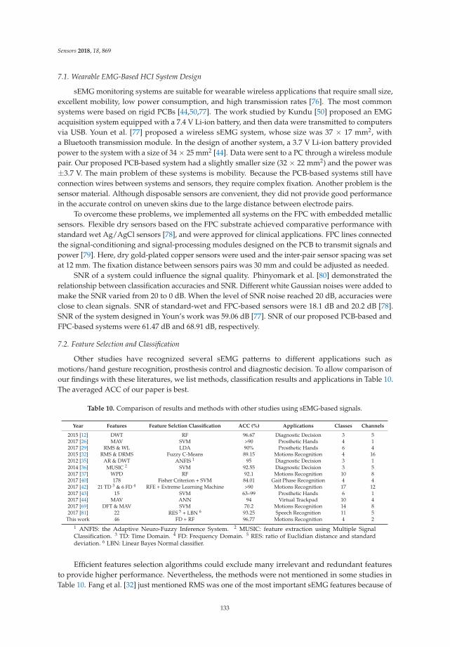
Sensors 2018, 18, 869

7.1. Wearable EMG-Based HCI System Design

sEMG monitoring systems are suitable for wearable wireless applications that require small size,excellent mobility, low power consumption, and high transmission rates [76]. The most commonsystems were based on rigid PCBs [44,50,77]. The work studied by Kundu [50] proposed an EMGacquisition system equipped with a 7.4 V Li-ion battery, and then data were transmitted to computersvia USB. Youn et al. [77] proposed a wireless sEMG system, whose size was 37 × 17 mm2, witha Bluetooth transmission module. In the design of another system, a 3.7 V Li-ion battery providedpower to the system with a size of 34 × 25 mm2 [44]. Data were sent to a PC through a wireless modulepair. Our proposed PCB-based system had a slightly smaller size (32 × 22 mm2) and the power was±3.7 V. The main problem of these systems is mobility. Because the PCB-based systems still haveconnection wires between systems and sensors, they require complex fixation. Another problem is thesensor material. Although disposable sensors are convenient, they did not provide good performancein the accurate control on uneven skins due to the large distance between electrode pairs.

To overcome these problems, we implemented all systems on the FPC with embedded metallicsensors. Flexible dry sensors based on the FPC substrate achieved comparative performance withstandard wet Ag/AgCl sensors [78], and were approved for clinical applications. FPC lines connectedthe signal-conditioning and signal-processing modules designed on the PCB to transmit signals andpower [79]. Here, dry gold-plated copper sensors were used and the inter-pair sensor spacing was setat 12 mm. The fixation distance between sensors pairs was 30 mm and could be adjusted as needed.

SNR of a system could influence the signal quality. Phinyomark et al. [80] demonstrated therelationship between classification accuracies and SNR. Different white Gaussian noises were added tomake the SNR varied from 20 to 0 dB. When the level of SNR noise reached 20 dB, accuracies wereclose to clean signals. SNR of standard-wet and FPC-based sensors were 18.1 dB and 20.2 dB [78].SNR of the system designed in Youn’s work was 59.06 dB [77]. SNR of our proposed PCB-based andFPC-based systems were 61.47 dB and 68.91 dB, respectively.

7.2. Feature Selection and Classification

Other studies have recognized several sEMG patterns to different applications such asmotions/hand gesture recognition, prosthesis control and diagnostic decision. To allow comparison ofour findings with these literatures, we list methods, classification results and applications in Table 10.The averaged ACC of our paper is best.

Table 10. Comparison of results and methods with other studies using sEMG-based signals.

Year Features Feature Selction Classification ACC (%) Applications Classes Channels

2015 [12] DWT RF 96.67 Diagnostic Decision 3 52017 [26] MAV SVM >90 Prosthetic Hands 4 12017 [29] RMS & WL LDA 90% Prosthetic Hands 6 42015 [32] RMS & DRMS Fuzzy C-Means 89.15 Motions Recognition 4 162012 [35] AR & DWT ANFIS 1 95 Diagnostic Decision 3 12014 [36] MUSIC 2 SVM 92.55 Diagnostic Decision 3 52017 [37] WPD RF 92.1 Motions Recognition 10 82017 [40] 178 Fisher Criterion + SVM 84.01 Gait Phase Recognition 4 42017 [42] 21 TD 3 & 6 FD 4 RFE + Extreme Learning Machine >90 Motions Recognition 17 122017 [43] 15 SVM 63–99 Prosthetic Hands 6 12017 [44] MAV ANN 94 Virtual Trackpad 10 42017 [69] DFT & MAV SVM 70.2 Motions Recognition 14 82017 [81] 22 RES 5 + LBN 6 93.25 Speech Recognition 11 5

This work 46 FD + RF 96.77 Motions Recognition 4 2

1 ANFIS: the Adaptive Neuro-Fuzzy Inference System. 2 MUSIC: feature extraction using Multiple SignalClassification. 3 TD: Time Domain. 4 FD: Frequency Domain. 5 RES: ratio of Euclidian distance and standarddeviation. 6 LBN: Linear Bayes Normal classifier.

Efficient features selection algorithms could exclude many irrelevant and redundant featuresto provide higher performance. Nevertheless, the methods were not mentioned in some studies inTable 10. Fang et al. [32] just mentioned RMS was one of the most important sEMG features because of

133

Sensors 2018, 18, 869

lower computational cost and decent performance. Another study used MAV for the same reason [44].The optimal features should be extracted by some criteria. Tosin et al. [42] demonstrated that RFE wasa powerful feature selection algorithm. However, the output was a list of ranks in separability withoutdetailed values. Then, quantitative feature selection methods including the Davies-Bouldin index [82],RES [81] and Fisher Criterion [40] were introduced. There are two problems in these methods. First,success rates of these methods are not high enough (Table 10). The second problem involves theoptimal number of features. Huang et al. [82] used a feature subset selected by the Davies-Bouldinindex to obtain 85% and 71% classification rates in offline and online tests, respectively. In Lee’swork, the authors tested classification performance fixing the numbers of feature subsets to 100 and150 [40]. In others, the feature selection process including CV of classifiers was complicated [81]. In ourpaper, the modified EC method was proposed because of low computational cost. We also combinedEuclidian distances with the Fisher’s discriminant to obtain the modified FD method. The accuraciesof these two methods were 96.66% and 96.77%, which were slightly better than the conventional RFEmethod and other feature selection methods in the table. The average number of features to receive thebest accuracy for each selected channel across all subjects was defined as the optimal feature number.This method was more reasonable than Lee’s work [40], and easier than Srisuwan’s work [81].

7.3. The Online Performance

Since the final target of our systems is for a wheelchair control, the performance of smartwheelchairs is compared and discussed in this section. Delicate motions of the upper limb controlledjoysticks-based smart wheelchairs [83], but they are not capable for patients with complete or partialloss of muscle activities. The EEG-based [83] and EOG-based [7] wheelchairs with automatednavigation systems were proposed. In Huang’s work [7], subjects could control the wheelchairto finish all tasks within 227 s and 277 s by joysticks and EOG signals, respectively. The recognitionrate for healthy subjects was 91.7%. The main challenge was to decrease misclassification rates ofunwanted blinks or rotational motions of eyes. In Zhang’s work [84], the destination selection was fast,but the critical problem was subjects needed 4.5 s to stop control.

The sEMG-based control method was considered in this work, because sEMG signals couldachieve higher accuracies and use in long-term applications. The fixed-moving paradigm couldimprove safety. The average time was 46.02 s, which means each vehicle motion including thesEMG-recognition and vehicle-moving periods cost 1.05 s. The waiting time was much shorter thanthe same method in an EEG-based wheelchair [85].

According to Kucukyildiz’s work [86], the fixed-moving control paradigm had challenges forpaths with frequently directional changes. Their work used very short analysis window (50 ms) forthe sEMG control. Englehart et al. analyzed the effects of analysis window length upon classificationaccuracy [74]. The results showed that the best performance is with 32 ms analysis window witha majority vote decision. There was no differences when the window length ranged from 32 ms to256 ms. However, in single-window analysis, the accuracy degraded rapidly with decreasing analysiswindow length. According to this work, the real-time processing window is 125 ms in our work.

To improve control’s continuity, the channel-combination and state-machine paradigms wereintroduced. The travel time of controlling by joysticks was 45.18 s. Subjects used 49.06 s and48.08 s by these two continuous sEMG-based paradigms. The accuracy of Paradigm 2 was 94.79%.The recognition rate of motions was 91.77% in Paradigm 3. The same comparisons were shown inKundu’s work [50]. The travel time of a designed wheelchair was 67.18 s and 72.88 s for joysticks andsEMG signals. The real time recognition accuracy was 90.58%. Despite the moving speed was lowerand the path length was shorter in our work, the real-time results were acceptable.

The trend of sEMG-based HCIs is to increase the degree-of-freedoms. Maeda et al. designedan omnidirectional wheelchair with four-channel sEMG signals [87]. They adopted amplitudecombinations of different channels during straining muscles. The similar method was defined asproportional control [48]. The performance in classifying 10 functions with a linear discriminant

134

Sensors 2018, 18, 869

classifier, reaching 94%, 93% and 87% at 16, 8 and 4 channels, respectively. In Ishii’s work [49],the combinations of different motions corresponded to eight control commands based on thestate machines.

In our work, Paradigm 3 and 4 were similar with the proportional and state-machine control.Our vehicle could move to five directions with two channels. The travel time of Paradigm 4 wasslightly shorter than Paradigm 3. These two paradigms were more sophisticated than Paradigm 2, butthey were closer to the real-life control method. However, these paradigms were hard to remember orimplement for some subjects, especially for the high-dimensional control.

7.4. Limitations and Future Work

There are several basic limitations associated with this study that need further development toprovide the wearable sEMG system for clinical purposes. (1) Although we obtained a stable acquisitionsystem, Balouchestni et al. [76] designed a system to recover the original bio-signals with good levelof accuracy and SNR greater than 95.8 dB. Therefore, the circuit architecture optimization are stillneeded. (2) From Table 10, the next step of research should extend the motion pool. (3) The currentresearch study recorded and analyzed the sEMG data performed only by healthy subjects. (4) In thefuture, minimization of analysis windows and improvement of single-window performance are mainworks for real-time algorithms. (5) In this study, subjects controlled the designed telecar in a laboratoryenvironment. We are combining our system with a smart wheelchair. To control it in a complicatedreal scenario, efforts still need to be made.

8. Conclusions

Two wearable sEMG acquisition systems are designed and implemented successfully in this work.The PCB-based prototype can capture four-channel sEMG signals simultaneously from differentforearm muscles, and the FPC-based system with two channels are utilized for online control.The system could communicate with a laptop wirelessly through Bluetooth. The high SNR of 61.47 dBand 68.91 dB for these systems ensure the signal quality. Temporal and frequency responses indicatethat the system can remove noise and are stable during all motions.

The ECU and ECR channels are selected with 97.45% and 96.55% mean classification accuraciesacross all pairs of motions and subjects. In single-channel analysis, the FD and RFE methods achievethe optimal accuracy with significantly less features than the EC method (p = 0.002 and p = 0.003respectively). For the channel ECU, the average accuracy increases to 97.82% with only 14 features.Accuracies above 98% are achieved comparing the REST state with other states. The FD methodproduces recognition rates in the range of 94.72% to 98.16% comparing among three motions.

Detailed features are selected according to the level of feature separability provided by the EC, FDand RFE methods. According to qualitative and quantitative weighting analysis, these three methodsopt for 31, 23 and 33 features, respectively. The feature selection results also prove that time-domainand time-frequency-domain features provide more discriminative information than frequency-domainfeatures. The FD-based feature subset with RF classifier achieves 96.77% accuracy, which is better thanother methods and single-type features referred in some references.

Furthermore, to validate the feasibility of proposed methods, we invited same group of subjectsto control the designed toy vehicle using four different paradigms. Subjects can accomplish the onlinetask by joysticks with averaged 45.18 s. For the fixed-moving paradigm, the mean travel time is 46.02 swith 94.79% recognition rate. The results of Paradigm 3 and 4 reveal that these paradigms can improvethe maneuverability and provide potentials in more sophisticated paths.

Therefore, all mentioned results suggest that our proposed acquisition systems and algorithmscan be used in the HCI research. The future work focuses on recording and discerning more motionsto realize the accurate implementation of smart wheelchairs.

135

Sensors 2018, 18, 869

Acknowledgments: The authors appreciate anonymous reviewers for their valuable comments, and F. Bahariand B. Gluckman for their technical and editorial assistance. This work was supported by the National KeyResearch and Development Program of China (No. 2016YFB0401201), the National Science Foundation of China(No. 61505028), and Enterprises, Universities and Research Institutes Prospective Joint Research Program ofJiangsu Province (No. BY2016076-07).

Author Contributions: Xi.Z. and H.S. conceived and designed the experiments; Ya.Z. and Z.F. designed theacquisition systems; Xu.Z. performed the statistical analysis; Yu.Z. and H.S. proposed the algorithms and analyzedthe data; H.S. wrote the paper; Xi.Z. reviewed the paper.

Conflicts of Interest: The authors declare no conflict of interest.

References

1. Skavhaug, I.M.; Lyons, K.R.; Nemchuk, A.; Muroff, S.D.; Joshi, S.S. Learning to modulate the partial powersof a single sEMG power spectrum through a novel human-computer interface. Hum. Mov. Sci. 2016, 47,60–69. [CrossRef] [PubMed]

2. Fukuda, O.; Tsuji, T.; Kaneko, M.; Otsuka, A. A human-assisting manipulator teleoperated by EMG signalsand arm motions. IEEE Trans. Robot. Autom. 2003, 19, 210–222. [CrossRef]

3. Wu, J.; Sun, L.; Jafari, R. A wearable system for recognizing American sign language in real-time using IMUand surface EMG sensors. IEEE J. Biomed. Health Inform. 2016, 20, 1281–1290. [CrossRef] [PubMed]

4. Galán, F.; Nuttin, M.; Lew, E.; Ferrez, P.W.; Vanacker, G.; Philips, J.; Millán, J.D.R. A brain-actuatedwheelchair: Asynchronous and non-invasive brain–computer interfaces for continuous control of robots.Clin. Neurophysiol. 2008, 119, 2159–2169. [CrossRef] [PubMed]

5. Ang, K.K.; Guan, C. EEG-based strategies to detect motor imagery for control and rehabilitation. IEEE Trans.

Neural Syst. Rehabil. Eng. 2017, 25, 392–401. [CrossRef] [PubMed]6. Barea, R.; Boquete, L.; Mazo, M.; López, E. Wheelchair guidance strategies using EOG. J. Intell. Robot. Syst.

2002, 34, 279–299. [CrossRef]7. Huang, Q.; He, S.; Wang, Q.; Gu, Z.; Peng, N.; Li, K.; Zhang, Y.; Shao, M.; Li, Y. An EOG-based

human-machine interface for wheelchair control. IEEE Trans. Biomed. Eng. 2017. [CrossRef] [PubMed]8. Pfurtscheller, G.; Allison, B.Z.; Brunner, C.; Bauernfeind, G.; Solis-Escalante, T.; Scherer, R.; Zander, T.O.;

Mueller-Putz, G.; Neuper, C.; Birbaumer, N. The hybrid BCI. Front. Neurosci. 2010, 4, 42. [CrossRef] [PubMed]9. Kawase, T.; Sakurada, T.; Koike, Y.; Kansaku, K. A hybrid BMI-based exoskeleton for paresis: EMG control

for assisting arm movements. J. Neural Eng. 2017, 14, 016015. [CrossRef] [PubMed]10. De Venuto, D.; Annese, V.F.; de Tommaso, M.; Vecchio, E.; Vincentelli, A.L. Combining EEG and EMG signals

in a wireless system for preventing fall in neurodegenerative diseases. In Ambient Assisted Living; Andò, B.,Siciliano, P., Marletta, V., Monteriù, A., Eds.; Springer International Publishing: Cham, Switzerland, 2015;Volume 11, pp. 317–327.

11. Lin, K.; Cinetto, A.; Wang, Y.; Chen, X.; Gao, S.; Gao, X. An online hybrid BCI system based on SSVEP andEMG. J. Neural Eng. 2016, 13, 026020. [CrossRef] [PubMed]

12. Gokgoz, E.; Subasi, A. Comparison of decision tree algorithms for EMG signal classification using DWT.Biomed. Signal Process. Control 2015, 18, 138–144. [CrossRef]

13. Stepp, C.E. Surface electromyography for speech and swallowing systems: Measurement, analysis, andinterpretation. J. Speech Lang. Hear. Res. 2012, 55, 1232–1246. [CrossRef]

14. Mishra, V.K.; Bajaj, V.; Kumar, A. Classification of normal, ALS, and myopathy EMG signals usingELM classifier. In Proceedings of the 2016 2nd International Conference on Advances in Electrical,Electronics, Information, Communication and Bio-Informatics (AEEICB), Chennai, India, 27–28 February2016; pp. 455–459.

15. Beniczky, S.; Conradsen, I.; Henning, O.; Fabricius, M.; Wolf, P. Automated real-time detection of tonic-clonicseizures using a wearable EMG device. Neurology 2018, 90, e1–e7. [CrossRef] [PubMed]

16. Szabó, C.Á.; Morgan, L.C.; Karkar, K.M.; Leary, L.D.; Lie, O.V.; Girouard, M.; Cavazos, J.E.Electromyography-based seizure detector: Preliminary results comparing a generalized tonic-clonic seizuredetection algorithm to video-EEG recordings. Epilepsia 2015, 56, 1432–1437. [CrossRef] [PubMed]

17. Xi, X.; Tang, M.; Miran, S.M.; Luo, Z. Evaluation of feature extraction and recognition for activity monitoringand fall detection based on wearable sEMG sensors. Sensors 2017, 17, 1229. [CrossRef] [PubMed]

136

Sensors 2018, 18, 869

18. Du, Y.; Jin, W.; Wei, W.; Hu, Y.; Geng, W. Surface EMG-based inter-session gesture recognition enhanced bydeep domain adaptation. Sensors 2017, 17, 458. [CrossRef] [PubMed]

19. Chen, Z.; Zhang, N.; Wang, Z.; Zhou, Z.; Hu, D. Hand gestures recognition from multi-channel forearmEMG signals. In Proceeding of the International Conference on Cognitive Systems and Signal Processing,Beijing, China, 19–23 November 2016; pp. 119–125.

20. Cheng, J.; Chen, X.; Liu, A.; Peng, H. A novel phonology-and radical-coded Chinese sign languagerecognition framework using accelerometer and surface electromyography sensors. Sensors 2015, 15,23303–23324. [CrossRef] [PubMed]

21. Kang, H.; Wang, W.; Li, X.; Du, H.; Li, L.; Ma, J. Multichannel s-EMG system of masticatory muscles: Designand clinical application in diagnosis of dysfunction in stomatognathic system. Biomed. Eng. Appl. Basis

Commun. 2015, 27, 1550008. [CrossRef]22. Yamaguchi, T.; Mikami, S.; Saito, M.; Okada, K.; Gotouda, A. A newly developed ultraminiature wearable

electromyogram system useful for analyses of masseteric activity during the whole day. J. Prosthodont. Res.

2018, 62, 110–115. [CrossRef] [PubMed]23. Hu, X.; Wang, Z.Z.; Ren, X.M. Classification of forearm action surface EMG signals based on fractal dimension.

J. Southeast Univ. 2005, 21, 324–329.24. Michieletto, S.; Tonin, L.; Antonello, M.; Bortoletto, R.; Spolaor, F.; Pagello, E.; Menegatti, E. GMM-based

single-joint angle estimation using EMG signals. In Proceedings of the 13th International Conference ofIntelligent Autonomous Systems, Padova, Italy, 15–18 July 2014; pp. 1173–1184.

25. Chen, X.; Wang, Z.J. Pattern recognition of number gestures based on a wireless surface EMG system.Biomed. Signal Process. Control 2013, 8, 184–192. [CrossRef]

26. Tavakoli, M.; Benussi, C.; Lourenco, J.L. Single channel surface EMG control of advanced prosthetic hands:A simple, low cost and efficient approach. Expert Syst. Appl. 2017, 79, 322–332. [CrossRef]

27. Pantelopoulos, A.; Bourbakis, N.G. A survey on wearable sensor-based systems for health monitoring andprognosis. IEEE Trans. Syst. Man Cybern. C 2010, 40, 1–12. [CrossRef]

28. Roland, T.; Baumgartner, W.; Amsuess, S.; Russold, M.F. Signal evaluation of capacitive EMG for upperlimb prostheses control using an ultra-low-power microcontroller. In Proceedings of the 2016 IEEE EMBSConference on Biomedical Engineering and Sciences (IECBES), Kuala Lumpur, Malaysia, 4–8 December2016; pp. 317–320.

29. Xiong, P.; Wu, C.; Zhou, H.; Song, A.; Hu, L.; Liu, X.P. Design of an accurate end-of-arm force display systembased on wearable arm gesture sensors and EMG sensors. Inform. Fusion 2018, 39, 178–185. [CrossRef]

30. Mejic, L.; Došen, S.; Ilic, V.; Stanišic, D.; Jorgovanovic, N. An implementation of movement classification forprosthesis control using custom-made EMG system. Serbian J. Electr. Eng. 2017, 14, 13–22. [CrossRef]

31. Costa, Á.; Itkonen, M.; Yamasaki, H.; Alnajjar, F.S.; Shimoda, S. Importance of muscle selection for EMGsignal analysis during upper limb rehabilitation of stroke patients. In Proceedings of the 2017 39th AnnualInternational Conference of the IEEE on Engineering in Medicine and Biology Society (EMBC), Seogwipo,Korea, 11–15 July 2017; pp. 2510–2513.

32. Fang, Y.; Liu, H.; Li, G.; Zhu, X. A multichannel surface EMG system for hand motion recognition. Int. J.

Hum. Robot. 2015, 12, 1550011. [CrossRef]33. Chen, H.; Zhang, Y.; Zhang, Z.; Fang, Y.; Liu, H.; Yao, C. Exploring the relation between EMG sampling

frequency and hand motion recognition accuracy. In Proceedings of the 2017 IEEE International Conferenceon Systems, Man and Cybernetics (SMC), Banff, AB, Canada, 5–8 October 2017.

34. Alkan, A.; Günay, M. Identification of EMG signals using discriminant analysis and SVM classifier.Expert Syst. Appl. 2012, 39, 44–47. [CrossRef]

35. Subasi, A. Classification of EMG signals using combined features and soft computing techniques.Appl. Soft Comput. 2012, 12, 2188–2198. [CrossRef]

36. Gokgoz, E.; Subasi, A. Effect of multiscale PCA de-noising on EMG signal classification for diagnosis ofneuromuscular disorders. J. Med. Syst. 2014, 38, 31. [CrossRef] [PubMed]

37. Abdullah, A.A.; Subasi, A.; Qaisar, S.M. Surface EMG signal classification by using WPD and ensembletree classifiers. In Proceedings of the International Conference on Medical and Biological Engineering 2017,Sarajevo, Bosnia and Herzegovina, 16–18 March 2017; pp. 475–481.

38. Wang, G.; Wang, Z.; Chen, W.; Zhuang, J. Classification of surface EMG signals using optimal wavelet packetmethod based on Davies-Bouldin criterion. Med. Biol. Eng. Comput. 2006, 44, 865–872. [CrossRef] [PubMed]

137

Sensors 2018, 18, 869

39. Lai, C.; Guo, S.; Cheng, L.; Wang, W. A comparative study of feature selection methods for the discriminativeAnalysis of Temporal Lobe Epilepsy. Front. Neurol. 2017, 8, 1–13. [CrossRef] [PubMed]

40. Lee, S.W.; Yi, T.; Jung, J.W.; Bien, Z. Design of a gait phase recognition system that can cope with EMGelectrode location variation. IEEE Trans. Autom. Sci. Eng. 2017, 14, 1429–1439. [CrossRef]

41. Wu, J.; Tian, Z.; Sun, L.; Estevez, L.; Jafari, R. Real-time American sign language recognition using wrist-wornmotion and surface EMG sensors. In Proceedings of the 2015 IEEE 12th International Conference on Wearableand Implantable Body Sensor Networks, Cambridge, MA, USA, 9–12 June 2015; pp. 1–6.

42. Tosin, M.C.; Majolo, M.; Chedid, R.; Cene, V.H.; Balbinot, A. sEMG feature selection and classification usingSVM-RFE. In Proceedings of the 2017 39th Annual International Conference of the IEEE Engineering inMedicine and Biology Society, Seogwipo, Korea, 11–15 July 2017; pp. 390–393.

43. Gailey, A.; Artemiadis, P.; Santello, M. Proof of concept of an online EMG-based decoding of hand posturesand individual digit forces for prosthetic hand control. Front. Neurol. 2017, 8, 7. [CrossRef] [PubMed]

44. Liu, X.; Sacks, J.; Zhang, M.; Richardson, A.G.; Lucas, T.H.; Van der Spiegel, J. The virtual trackpad:An electromyography-based, wireless, real-time, low-power, embedded hand-gesture-recognition systemusing an event-driven artificial neural network. IEEE Trans. Circuits Syst. II Express Briefs 2017, 64, 1257–1261.[CrossRef]

45. Simpson, R.C. Smart wheelchairs: A literature review. J. Rehabil. Res. Dev. 2005, 42, 423–436. [CrossRef][PubMed]

46. Lung, C.W.; Chen, C.L.; Jan, Y.K.; Chao, L.F.; Chen, W.F.; Liau, B.Y. Activation sequence patterns of forearmmuscles for driving a power wheelchair. In Proceedings of the International Conference on Applied HumanFactors and Ergonomics, Los Angeles, CA, USA, 17–21 July 2017; pp. 141–147.

47. Al-Okby, M.F.R.; Neubert, S.; Stoll, N.; Thurow, K. Development and testing of intelligent low-cost wheelchaircontroller for quadriplegics and paralysis patients. In Proceedings of the 2017 2nd International Conferenceon Bio-engineering for Smart Technologies (BioSMART), Paris, France, 30 August–1 September 2017; pp. 1–4.

48. Parker, P.; Englehart, K.; Hudgins, B. Myoelectric signal processing for control of powered limb prostheses.J. Electromyogr. Kinesiol. 2006, 16, 541–548. [CrossRef] [PubMed]

49. Ishii, C.; Konishi, R. A control of electric wheelchair using an emg based on degree of muscular activity.In Proceedings of the 2016 Euromicro Conference on Digital System Design (DSD), Limassol, Cyprus,31 August–2 September 2016; pp. 567–574.

50. Kundu, A.S.; Mazumder, O.; Lenka, P.K.; Bhaumik, S. Hand gesture recognition based omnidirectionalwheelchair control using IMU and EMG sensors. J. Intell. Robot. Syst. 2017, 1–13. [CrossRef]

51. Shi, J.; Ren, X.; Liu, Z.; Chen, Z.; Duan, F. The development of a wheelchair control method based onsEMG signals. In Proceedings of the 2017 Chinese Intelligent Systems Conference, Mudanjiang, China,14–15 October 2017; pp. 429–438.

52. Duun-Henriksen, J.; Kjaer, T.W.; Madsen, R.E.; Remvig, L.S.; Thomsen, C.E.; Sorensen, H.B.D.Channel selection for automatic seizure detection. Clin. Neurophysiol. 2012, 123, 84–92. [CrossRef] [PubMed]

53. Xu, J.; Mitra, S.; Van Hoof, C.; Yazicioglu, R.F.; Makinwa, K.A. Active electrodes for wearable EEG acquisition:Review and electronics design methodology. IEEE Rev. Biomed. Eng. 2017, 10, 187–198. [CrossRef] [PubMed]

54. Merletti, R.; Botter, A.; Troiano, A.; Merlo, E.; Minetto, M.A. Technology and instrumentation for detectionand conditioning of the surface electromyographic signal: State of the art. Clin. Biomech. 2009, 24, 122–134.[CrossRef] [PubMed]

55. Chi, Y.M.; Jung, T.P.; Cauwenberghs, G. Dry-contact and noncontact biopotential electrodes:Methodological review. IEEE Rev. Biomed. Eng. 2010, 3, 106–119. [CrossRef] [PubMed]

56. Merletti, R.; Hermens, H. Detection and conditioning of the surface EMG signal. In Electromyography:

Physiology, Engineering and Noninvasive Applications; Merletti, R., Parker, P.A., Eds.; IEEE Press and John Wiley& Sons: Hoboken, NJ, USA, 2004; pp. 107–132. ISBN 0-471-67580-6.

57. Oskoei, M.A.; Hu, H. Support vector machine-based classification scheme for myoelectric control applied toupper limb. IEEE Trans. Biomed. Eng. 2008, 55, 1956–1965. [CrossRef] [PubMed]

58. Bakshi, B.R. Multiscale PCA with application to multivariate statistical process monitoring. AIChE J. 1998,44, 1596–1610. [CrossRef]

59. Sheriff, M.Z.; Mansouri, M.; Karim, M.N.; Nounou, M. Fault detection using multiscale PCA-based movingwindow GLRT. J. Process Control 2017, 54, 47–64. [CrossRef]

138

Sensors 2018, 18, 869

60. Alickovic, E.; Subasi, A. Effect of multiscale PCA de-noising in ECG beat classification for diagnosis ofcardiovascular diseases. Circuits Syst. Signal Process. 2015, 34, 513–533. [CrossRef]

61. Zhang, M.; Sawchuk, A.A. Human daily activity recognition with sparse representation using wearablesensors. IEEE J. Biomed. Health Inform. 2013, 17, 553–560. [CrossRef] [PubMed]

62. Xu, Q.; Zhou, H.; Wang, Y.; Huang, J. Fuzzy support vector machine for classification of EEG signals usingwavelet-based features. Med. Eng. Phys. 2009, 31, 858–865. [CrossRef] [PubMed]

63. Guyon, I.; Elisseeff, A. An introduction to variable and feature selection. J. Mach. Learn. Res. 2003, 3,1157–1182.

64. Schiff, S.J.; Sauer, T.; Kumar, R.; Weinstein, S.L. Neuronal spatiotemporal pattern discrimination:The dynamical evolution of seizures. Neuroimage 2005, 28, 1043–1055. [CrossRef] [PubMed]

65. Akata, Z.; Perronnin, F.; Harchaoui, Z.; Schmid, C. Good practice in large-scale learning for imageclassification. IEEE Trans. Pattern Anal. Mach. Intell. 2014, 36, 507–520. [CrossRef] [PubMed]

66. Yin, Z.; Wang, Y.; Liu, L.; Zhang, W.; Zhang, J. Cross-subject EEG feature selection for emotion recognitionusing transfer recursive feature elimination. Front. Neurorobot. 2017, 11, 19. [CrossRef] [PubMed]

67. Zhou, X.; Tuck, D.P. MSVM-RFE: Extensions of SVM-RFE for multiclass gene selection on DNA microarraydata. Bioinformatics 2007, 23, 1106–1114. [CrossRef] [PubMed]

68. Wan, B.; Wu, R.; Zhang, K.; Liu, L. A new subtle hand gestures recognition algorithm based on EMG andFSR. In Proceedings of the 2017 IEEE 21st International Conference on Computer Supported CooperativeWork in Design (CSCWD), Wellington, New Zealand, 26–28 April 2017; pp. 127–132.

69. Zhang, H.; Yang, D.; Shi, C.; Jiang, L.; Liu, H. Robust EMG pattern recognition with electrodedonning/doffing and multiple confounding factors. In Proceedings of the International Conference onIntelligent Robotics and Applications, Wuhan, China, 16–18 August 2017; pp. 413–424.

70. Kondo, G.; Kato, R.; Yokoi, H.; Arai, T. Classification of individual finger motions hybridizingelectromyogram in transient and converged states. In Proceedings of the 2010 IEEE International Conferenceon Robotics and Automation (ICRA), Anchorage, AK, USA, 3–7 May 2010; pp. 2909–2915.

71. Liaw, A.; Wiener, M. Classification and regression by random forest. R News 2002, 2, 18–22.72. Breiman, L. Random forests. Mach. Learn. 2001, 45, 5–32. [CrossRef]73. Chang, C.C.; Lin, C.J. LIBSVM: A library for support vector machines. ACM Trans. Intell. Syst. Technol. 2011,

2, 1–27. [CrossRef]74. Englehart, K.; Hudgins, B. A robust, real-time control scheme for multifunction myoelectric control.

IEEE Trans. Biomed. Eng. 2003, 50, 848–854. [CrossRef] [PubMed]75. Dobrowolski, A.P.; Wierzbowski, M.; Tomczykiewicz, K. Multiresolution MUAPs decomposition and

SVM-based analysis in the classification of neuromuscular disorders. Comput. Methods Programs Biomed.

2011, 107, 393–403. [CrossRef] [PubMed]76. Balouchestani, M.; Krishnan, S. Effective low-power wearable wireless surface EMG sensor design based on

analog-compressed sensing. Sensors 2014, 14, 24305–24328. [CrossRef] [PubMed]77. Youn, W.; Kim, J. Development of a compact-size and wireless surface EMG measurement system.

In Proceedings of the ICROS-SICE International Joint Conference 2009, Fukuoka, Japan, 18–21 August2009; pp. 1625–1628.

78. Lin, K.; Wang, X.; Zhang, X.; Wang, B.; Huang, J.; Huang, F. An FPC based flexible dry electrode withstacked double-micro-domes array for wearable biopotential recording system. Microsyst. Technol. 2017, 23,1443–1451. [CrossRef]

79. Guo, W.; Yao, P.; Sheng, X.; Liu, H.; Zhu, X. A wireless wearable sEMG and NIRS acquisition system foran enhanced human-computer interface. In Proceedings of the 2014 IEEE International Conference onSystems, Man and Cybernetics, San Diego, CA, USA, 5–8 October 2014; pp. 2192–2197.

80. Phinyomark, A.; Phukpattaranont, P.; Limsakul, C. Feature reduction and selection for EMG signalclassification. Expert Syst. Appl. 2012, 39, 7420–7431. [CrossRef]

81. Srisuwan, N.; Phukpattaranont, P.; Limsakul, C. Comparison of feature evaluation criteria for speechrecognition based on electromyography. Med. Biol. Eng. Comput. 2017, 1–11. [CrossRef] [PubMed]

82. Huang, H.P.; Liu, Y.H.; Liu, L.W.; Wong, C.S. EMG classification for prehensile postures using cascadedarchitecture of neural networks with self-organizing maps. In Proceedings of the 2003 IEEE InternationalConference on Robotics & Automation, Taipei, Taiwan, 14–19 September 2003; Volume 1, pp. 1497–1502.

139

Sensors 2018, 18, 869

83. Cler, M.J.; Stepp, C.E. Discrete Versus Continuous Mapping of Facial Electromyography for Human–MachineInterface Control: Performance and Training Effects. IEEE Trans. Neural Syst. Rehabil. Eng. 2015, 23, 572–580.[CrossRef] [PubMed]

84. Zhang, R.; Li, Y.; Yan, Y.; Zhang, H.; Wu, S.; Yu, T.; Gu, Z. Control of a wheelchair in an indoor environmentbased on a brain–computer interface and automated navigation. IEEE Trans. Neural Syst. Rehabil. Eng. 2016,24, 128–139. [CrossRef] [PubMed]

85. Chin, Z.Y.; Ang, K.K.; Wang, C.; Guan, C. Navigation in a virtual environment using multiclass motorimagery Brain-Computer Interface. In Proceedings of the 2013 IEEE Symposium on the ComputationalIntelligence, Cognitive Algorithms, Mind, and Brain (CCMB), Singapore, 16–19 April 2013; pp. 152–157.

86. Kucukyildiz, G.; Ocak, H.; Karakaya, S.; Sayli, O. Design and implementation of a multi sensor based braincomputer interface for a robotic wheelchair. J. Intell. Robot. Syst. 2017, 87, 247–263. [CrossRef]

87. Maeda, Y.; Ishibashi, S. Operating instruction method based on EMG for omnidirectional wheelchairrobot. In Proceedings of the 2017 Joint 17th World Congress of International Fuzzy Systems Associationand 9th International Conference on Soft Computing and Intelligent Systems (IFSA-SCIS), Otsu, Japan,27–30 June 2017; pp. 1–5.

© 2018 by the authors. Licensee MDPI, Basel, Switzerland. This article is an open accessarticle distributed under the terms and conditions of the Creative Commons Attribution(CC BY) license (http://creativecommons.org/licenses/by/4.0/).

140

sensors

Article

Evaluating the Influence of Chromatic and LuminanceStimuli on SSVEPs from Behind-the-Ears andOccipital Areas

Alan Floriano 1,†, Pablo F. Diez 2,3 and Teodiano Freire Bastos-Filho 1,*

1 Postgraduate Program in Electrical Engineering, Federal University of Espirito Santo, Vitoria 29075-910,Brazil; afloriano.ufes@gmail.com

2 Gabinete de Tecnologia Medica (GATEME), Facultad de Ingenieria, Universidad Nacional de San Juan,San Juan J5400ARL, Argentina; pdiez@gateme.unsj.edu.ar

3 Consejo Nacional de Investigaciones Científicas y Técnicas (CONICET), San Juan C1425FBQ, Argentina* Correspondence: teodiano.bastos@ufes.br; Tel.: +55-27-4009-2077† Current address: Av. Fernando Ferrari, 514, Goiabeiras, Vitoria CEP 29075-910, Brazil.

Received: 30 November 2017; Accepted: 14 February 2018; Published: 17 February 2018

Abstract: This work presents a study of chromatic and luminance stimuli in low-, medium-,and high-frequency stimulation to evoke steady-state visual evoked potential (SSVEP) in thebehind-the-ears area. Twelve healthy subjects participated in this study. The electroencephalogram(EEG) was measured on occipital (Oz) and left and right temporal (TP9 and TP10) areas. The SSVEPwas evaluated in terms of amplitude, signal-to-noise ratio (SNR), and detection accuracy usingpower spectral density analysis (PSDA), canonical correlation analysis (CCA), and temporally localmultivariate synchronization index (TMSI) methods. It was found that stimuli based on suitablecolor and luminance elicited stronger SSVEP in the behind-the-ears area, and that the response of theSSVEP was related to the flickering frequency and the color of the stimuli. Thus, green-red stimuluselicited the highest SSVEP in medium-frequency range, and green-blue stimulus elicited the highestSSVEP in high-frequency range, reaching detection accuracy rates higher than 80%. These findingswill aid in the development of more comfortable, accurate and stable BCIs with electrodes positionedon the behind-the-ears (hairless) areas.

Keywords: SSVEP; visual stimuli; BCI; hairless area

1. Introduction

The elicited response in the visual cortex by light stimuli flickering at a constant frequency isknown as steady-state visual evoked potential (SSVEP) [1]. In the electroencephalogram (EEG), thesepotentials manifest as an oscillatory component in the signal, with the same frequency (and/orits harmonics) of the visual stimulation [1]. SSVEP can normally be evoked up to 90 Hz [2],and three stimuli bands can be identified: low (up to 12 Hz), medium (12–30 Hz), and high-frequency(≥30 Hz) [3–5].

SSVEPs have been used for studies concerning the brain, vision, and the development ofbrain–computer interfaces (BCIs) [6]. People with severe disabilities can use BCIs as an alternativechannel for interaction and communication with the environment around them, only using brainactivity [7]. In SSVEP-based BCIs, each stimulus flickers at a specified frequency [8]. Thus, when aperson gazes at one of the stimuli, an SSVEP is evoked in the brain [6,9], which can be detected in theEEG signal, and later translated into a control command [10].

Researches have used the SSVEP response to develop assistive technologies, such asrobotic wheelchairs [11,12] and robotic exoskeletons [13], as well as for rehabilitation [14,15],

Sensors 2018, 18, 615; doi:10.3390/s18020615 www.mdpi.com/journal/sensors141

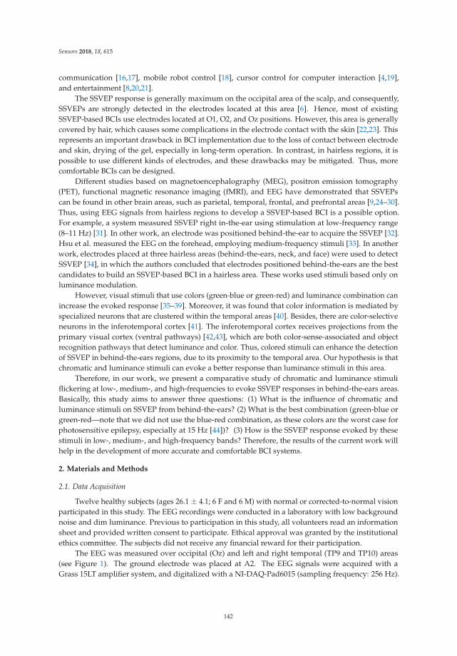
Sensors 2018, 18, 615

communication [16,17], mobile robot control [18], cursor control for computer interaction [4,19],and entertainment [8,20,21].

The SSVEP response is generally maximum on the occipital area of the scalp, and consequently,SSVEPs are strongly detected in the electrodes located at this area [6]. Hence, most of existingSSVEP-based BCIs use electrodes located at O1, O2, and Oz positions. However, this area is generallycovered by hair, which causes some complications in the electrode contact with the skin [22,23]. Thisrepresents an important drawback in BCI implementation due to the loss of contact between electrodeand skin, drying of the gel, especially in long-term operation. In contrast, in hairless regions, it ispossible to use different kinds of electrodes, and these drawbacks may be mitigated. Thus, morecomfortable BCIs can be designed.

Different studies based on magnetoencephalography (MEG), positron emission tomography(PET), functional magnetic resonance imaging (fMRI), and EEG have demonstrated that SSVEPscan be found in other brain areas, such as parietal, temporal, frontal, and prefrontal areas [9,24–30].Thus, using EEG signals from hairless regions to develop a SSVEP-based BCI is a possible option.For example, a system measured SSVEP right in-the-ear using stimulation at low-frequency range(8–11 Hz) [31]. In other work, an electrode was positioned behind-the-ear to acquire the SSVEP [32].Hsu et al. measured the EEG on the forehead, employing medium-frequency stimuli [33]. In anotherwork, electrodes placed at three hairless areas (behind-the-ears, neck, and face) were used to detectSSVEP [34], in which the authors concluded that electrodes positioned behind-the-ears are the bestcandidates to build an SSVEP-based BCI in a hairless area. These works used stimuli based only onluminance modulation.

However, visual stimuli that use colors (green-blue or green-red) and luminance combination canincrease the evoked response [35–39]. Moreover, it was found that color information is mediated byspecialized neurons that are clustered within the temporal areas [40]. Besides, there are color-selectiveneurons in the inferotemporal cortex [41]. The inferotemporal cortex receives projections from theprimary visual cortex (ventral pathways) [42,43], which are both color-sense-associated and objectrecognition pathways that detect luminance and color. Thus, colored stimuli can enhance the detectionof SSVEP in behind-the-ears regions, due to its proximity to the temporal area. Our hypothesis is thatchromatic and luminance stimuli can evoke a better response than luminance stimuli in this area.

Therefore, in our work, we present a comparative study of chromatic and luminance stimuliflickering at low-, medium-, and high-frequencies to evoke SSVEP responses in behind-the-ears areas.Basically, this study aims to answer three questions: (1) What is the influence of chromatic andluminance stimuli on SSVEP from behind-the-ears? (2) What is the best combination (green-blue orgreen-red—note that we did not use the blue-red combination, as these colors are the worst case forphotosensitive epilepsy, especially at 15 Hz [44])? (3) How is the SSVEP response evoked by thesestimuli in low-, medium-, and high-frequency bands? Therefore, the results of the current work willhelp in the development of more accurate and comfortable BCI systems.

2. Materials and Methods

2.1. Data Acquisition

Twelve healthy subjects (ages 26.1 ± 4.1; 6 F and 6 M) with normal or corrected-to-normal visionparticipated in this study. The EEG recordings were conducted in a laboratory with low backgroundnoise and dim luminance. Previous to participation in this study, all volunteers read an informationsheet and provided written consent to participate. Ethical approval was granted by the institutionalethics committee. The subjects did not receive any financial reward for their participation.

The EEG was measured over occipital (Oz) and left and right temporal (TP9 and TP10) areas(see Figure 1). The ground electrode was placed at A2. The EEG signals were acquired with aGrass 15LT amplifier system, and digitalized with a NI-DAQ-Pad6015 (sampling frequency: 256 Hz).

142

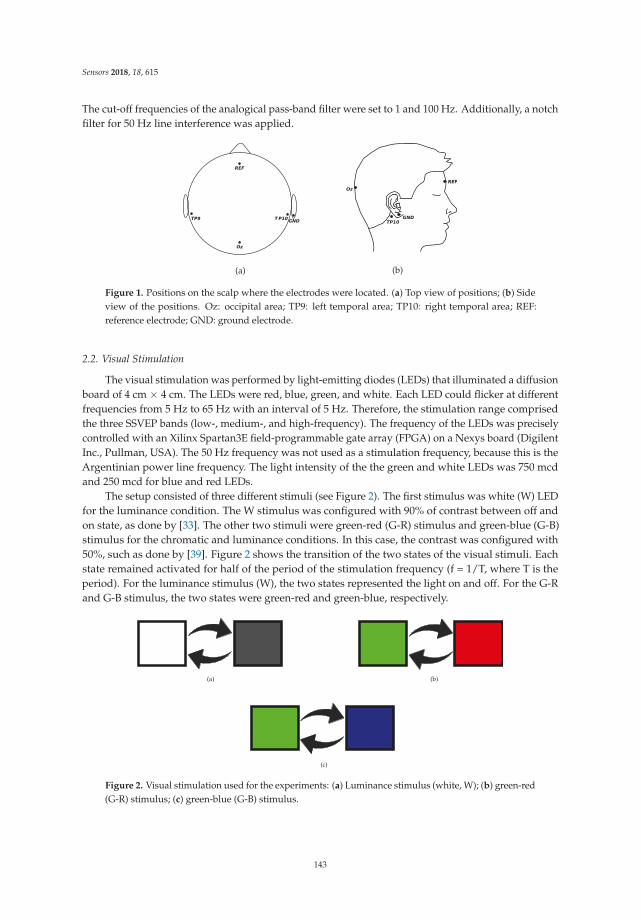
Sensors 2018, 18, 615

The cut-off frequencies of the analogical pass-band filter were set to 1 and 100 Hz. Additionally, a notchfilter for 50 Hz line interference was applied.

TP9 TP10

REF

Oz

GNDGND

TP10

Oz

REF

(a) (b)

Figure 1. Positions on the scalp where the electrodes were located. (a) Top view of positions; (b) Sideview of the positions. Oz: occipital area; TP9: left temporal area; TP10: right temporal area; REF:reference electrode; GND: ground electrode.

2.2. Visual Stimulation

The visual stimulation was performed by light-emitting diodes (LEDs) that illuminated a diffusionboard of 4 cm × 4 cm. The LEDs were red, blue, green, and white. Each LED could flicker at differentfrequencies from 5 Hz to 65 Hz with an interval of 5 Hz. Therefore, the stimulation range comprisedthe three SSVEP bands (low-, medium-, and high-frequency). The frequency of the LEDs was preciselycontrolled with an Xilinx Spartan3E field-programmable gate array (FPGA) on a Nexys board (DigilentInc., Pullman, USA). The 50 Hz frequency was not used as a stimulation frequency, because this is theArgentinian power line frequency. The light intensity of the the green and white LEDs was 750 mcdand 250 mcd for blue and red LEDs.

The setup consisted of three different stimuli (see Figure 2). The first stimulus was white (W) LEDfor the luminance condition. The W stimulus was configured with 90% of contrast between off andon state, as done by [33]. The other two stimuli were green-red (G-R) stimulus and green-blue (G-B)stimulus for the chromatic and luminance conditions. In this case, the contrast was configured with50%, such as done by [39]. Figure 2 shows the transition of the two states of the visual stimuli. Eachstate remained activated for half of the period of the stimulation frequency (f = 1/T, where T is theperiod). For the luminance stimulus (W), the two states represented the light on and off. For the G-Rand G-B stimulus, the two states were green-red and green-blue, respectively.

(a) (b)

(c)

Figure 2. Visual stimulation used for the experiments: (a) Luminance stimulus (white, W); (b) green-red(G-R) stimulus; (c) green-blue (G-B) stimulus.

143

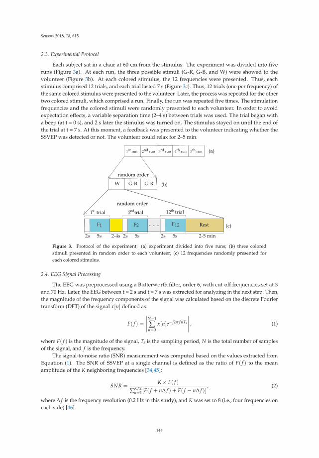
Sensors 2018, 18, 615

2.3. Experimental Protocol

Each subject sat in a chair at 60 cm from the stimulus. The experiment was divided into fiveruns (Figure 3a). At each run, the three possible stimuli (G-R, G-B, and W) were showed to thevolunteer (Figure 3b). At each colored stimulus, the 12 frequencies were presented. Thus, eachstimulus comprised 12 trials, and each trial lasted 7 s (Figure 3c). Thus, 12 trials (one per frequency) ofthe same colored stimulus were presented to the volunteer. Later, the process was repeated for the othertwo colored stimuli, which comprised a run. Finally, the run was repeated five times. The stimulationfrequencies and the colored stimuli were randomly presented to each volunteer. In order to avoidexpectation effects, a variable separation time (2–4 s) between trials was used. The trial began witha beep (at t = 0 s), and 2 s later the stimulus was turned on. The stimulus stayed on until the end ofthe trial at t = 7 s. At this moment, a feedback was presented to the volunteer indicating whether theSSVEP was detected or not. The volunteer could relax for 2–5 min.

2s 5s 2s 5s 2-5 min

W G-B G-R

1st trial 12th

. . .F1 F12 Rest

1st run 2nd run 3rd run 4th run 5th run (a)

(b)

(c)

random order

random order

trial

2-4s

F2

2s 5s

2ndtrial

Figure 3. Protocol of the experiment: (a) experiment divided into five runs; (b) three coloredstimuli presented in random order to each volunteer; (c) 12 frequencies randomly presented foreach colored stimulus.

2.4. EEG Signal Processing

The EEG was preprocessed using a Butterworth filter, order 6, with cut-off frequencies set at 3and 70 Hz. Later, the EEG between t = 2 s and t = 7 s was extracted for analyzing in the next step. Then,the magnitude of the frequency components of the signal was calculated based on the discrete Fouriertransform (DFT) of the signal x[n] defined as:

F( f ) =

∣∣∣∣∣N−1

∑n=0

x[n]e−j2π f nTs

∣∣∣∣∣ , (1)

where F( f ) is the magnitude of the signal, Ts is the sampling period, N is the total number of samplesof the signal, and f is the frequency.

The signal-to-noise ratio (SNR) measurement was computed based on the values extracted fromEquation (1). The SNR of SSVEP at a single channel is defined as the ratio of F( f ) to the meanamplitude of the K neighboring frequencies [34,45]:

SNR =K × F( f )

∑K/2n=1[F( f + n∆ f ) + F( f − n∆ f )]

, (2)

where ∆ f is the frequency resolution (0.2 Hz in this study), and K was set to 8 (i.e., four frequencies oneach side) [46].

144

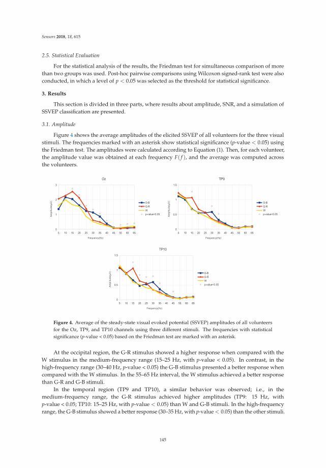
Sensors 2018, 18, 615

2.5. Statistical Evaluation

For the statistical analysis of the results, the Friedman test for simultaneous comparison of morethan two groups was used. Post-hoc pairwise comparisons using Wilcoxon signed-rank test were alsoconducted, in which a level of p < 0.05 was selected as the threshold for statistical significance.

3. Results

This section is divided in three parts, where results about amplitude, SNR, and a simulation ofSSVEP classification are presented.

3.1. Amplitude

Figure 4 shows the average amplitudes of the elicited SSVEP of all volunteers for the three visualstimuli. The frequencies marked with an asterisk show statistical significance (p-value < 0.05) usingthe Friedman test. The amplitudes were calculated according to Equation (1). Then, for each volunteer,the amplitude value was obtained at each frequency F( f ), and the average was computed acrossthe volunteers.

Figure 4. Average of the steady-state visual evoked potential (SSVEP) amplitudes of all volunteersfor the Oz, TP9, and TP10 channels using three different stimuli. The frequencies with statisticalsignificance (p-value < 0.05) based on the Friedman test are marked with an asterisk.

At the occipital region, the G-R stimulus showed a higher response when compared with theW stimulus in the medium-frequency range (15–25 Hz, with p-value < 0.05). In contrast, in thehigh-frequency range (30–40 Hz, p-value < 0.05) the G-B stimulus presented a better response whencompared with the W stimulus. In the 55–65 Hz interval, the W stimulus achieved a better responsethan G-R and G-B stimuli.

In the temporal region (TP9 and TP10), a similar behavior was observed; i.e., in themedium-frequency range, the G-R stimulus achieved higher amplitudes (TP9: 15 Hz, withp-value < 0.05; TP10: 15–25 Hz, with p-value < 0.05) than W and G-B stimuli. In the high-frequencyrange, the G-B stimulus showed a better response (30–35 Hz, with p-value < 0.05) than the other stimuli.

145

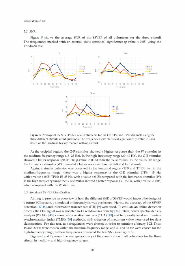
Sensors 2018, 18, 615

3.2. SNR

Figure 5 shows the average SNR of the SSVEP of all volunteers for the three stimuli.The frequencies marked with an asterisk show statistical significance (p-value < 0.05) using theFriedman test.

Figure 5. Average of the SSVEP SNR of all volunteers for the Oz, TP9, and TP10 channels using thethree different stimulus configurations. The frequencies with statistical significance (p-value < 0.05)based on the Friedman test are marked with an asterisk.

At the occipital region, the G-R stimulus showed a higher response than the W stimulus inthe medium-frequency range (15–25 Hz). In the high-frequency range (30–40 Hz), the G-B stimulusshowed a better response (30–35 Hz, p-value < 0.05) than the W stimulus. In the 55–65 Hz range,the luminance stimulus (W) presented a better response than the G-R and G-B stimuli.

Again, a similar behavior was observed in the temporal region (TP9 and TP10); i.e., in themedium-frequency range, there was a higher response of the G-R stimulus (TP9: 15 Hz,with p-value < 0.05; TP10: 15–25 Hz, with p-value < 0.05) compared with the luminance stimulus (W).In the high-frequency range the G-B stimulus showed a better response (30–35 Hz, with p-value < 0.05)when compared with the W stimulus.

3.3. Simulated SSVEP Classification

Aiming to provide an overview of how the different SNR of SSVEP would impact the design ofa future BCI system, a simulated online analysis was performed. Hence, the accuracy of the SSVEPdetection [47,48] and information transfer rate (ITR) [9] were used. To emulate an online detectionprocess, the EEG signal was segmented in 4 s windows (as done by [34]). Then, power spectral densityanalysis (PSDA) [45], canonical correlation analysis (CCA) [49] and temporally local multivariatesynchronization index (TMSI) [50] methods, with criterion of maximum value were used for dataclassification. For this test, two frequencies were chosen in order to simulate a binary BCI. Thus,15 and 20 Hz were chosen within the medium-frequency range, and 30 and 35 Hz were chosen for thehigh-frequency range, as these frequencies presented the best SNR (see Figure 5).

Figures 6 and 7 present the average accuracy of the classification of all volunteers for the threestimuli in medium- and high-frequency ranges.

146

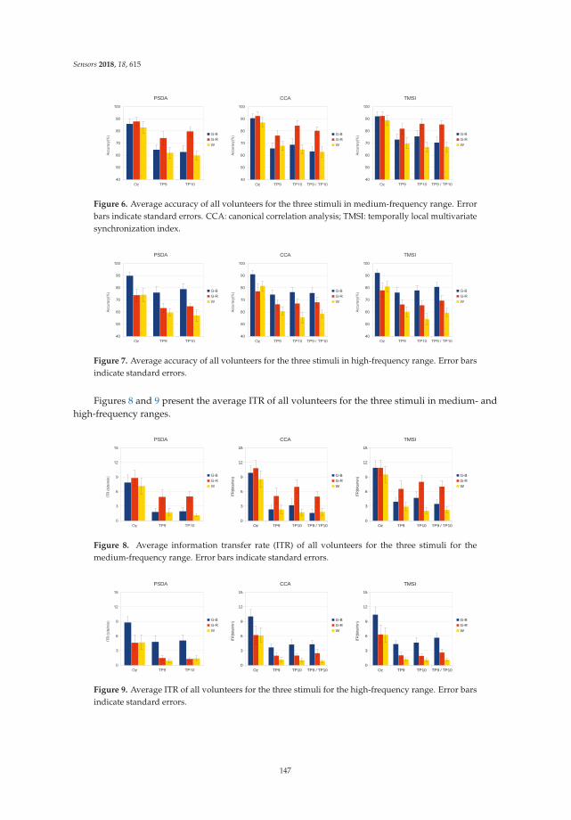
Sensors 2018, 18, 615

Figure 6. Average accuracy of all volunteers for the three stimuli in medium-frequency range. Errorbars indicate standard errors. CCA: canonical correlation analysis; TMSI: temporally local multivariatesynchronization index.

Figure 7. Average accuracy of all volunteers for the three stimuli in high-frequency range. Error barsindicate standard errors.

Figures 8 and 9 present the average ITR of all volunteers for the three stimuli in medium- andhigh-frequency ranges.

Figure 8. Average information transfer rate (ITR) of all volunteers for the three stimuli for themedium-frequency range. Error bars indicate standard errors.

Figure 9. Average ITR of all volunteers for the three stimuli for the high-frequency range. Error barsindicate standard errors.

147

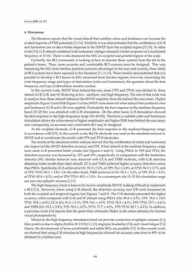
Sensors 2018, 18, 615

4. Discussion

The literature reports that the visual stimuli that combine colors and luminance can increase theevoked response of P300 potentials [35,36]. Similarly, it was demonstrated that the combination of G-Band luminance can evoke a better response in the SSVEP from the occipital region [37,38]. In otherwork [39], G-R stimuli combined with luminance changes obtained a better response at a modulatedfrequency of 15 Hz. These works measured the EEG on occipital and parietal regions of the scalp.

Currently, the BCI community is looking at how to transfer these systems from the lab to thepatient’s home. Thus, more accurate and comfortable BCI systems must be designed. This way,measuring the EEG from hairless positions presents advantages to the user, and recently, these kindsof BCI systems have been reported in the literature [31,32,34]. These studies demonstrated that it ispossible to develop a BCI based on EEG measured from hairless regions; however, concerning thewide frequency range and types of stimulation (color and luminance), the question about the bestfrequency and type of stimulation remains unclear.

In the current work, SSVEP from behind-the-ears areas (TP9 and TP10) was elicited by threestimuli (G-B, G-R, and W) flickering at low-, medium-, and high-frequency. The aim of this work wasto analyze how these stimuli influence the SSVEP response from the behind-the-ears areas. Higheramplitude (Figure 4) and SNR (Figure 5) of the SSVEP were observed when stimuli that combined colorand luminance (G-R and G-B) were applied. Particularly, the best response in the medium-frequencyband (15–25 Hz) was obtained with G-R stimulation. On the other hand, G-B stimulation showedthe best response in the high-frequency range (30–40 Hz). Therefore, a suitable color and luminancestimulation allows the achievement of higher amplitudes and higher SNR from behind-the-ears areas,and consequently, an accurate and comfortable BCI may be designed.

At the occipital electrode, G-R presented the best response in the medium-frequency range,in accordance with [39]. In the current work, the Oz electrode was used as the standard measure inSSVEP and to corroborate the results with TP9 and TP10 electrodes.

The results of the simulated online analysis showed that the combination of colors and luminancealso improved the SSVEP detection accuracy and ITR. When stimuli in the medium-frequency rangewere used, G-R presented better results (see Figures 6 and 8). Using PSDA in TP9 and TP10, thedetection accuracy was increased by 12% and 19%, respectively, in comparison with the luminancestimulus (W). Similar behavior was observed with CCA and TMSI methods, with G-R stimulusobtaining better results than other stimuli. CCA and TMSI achieved higher accuracy detection valuesthan PSDA. Specifically, CCA achieved at Oz: 92.3± 3.0%, at TP9: 76.1± 4.8%, at TP10: 84.3± 3.7%, andat TP9/TP10: 80.2 ± 2.8%. On the other hand, TMSI achieved at Oz: 92.3 ± 3.2%, at TP9: 81.8 ± 4.2%,at TP10: 85.8 ± 4.2%, and at TP9/TP10: 85.3 ± 3.3%. As a counterpart, the 15–25 Hz stimulation rangecan provoke epileptic seizures [1,51].

The high-frequency band is known for its low-amplitude SSVEP, making difficult to implementa BCI [52]. However, when using G-B stimuli, the detection accuracy and ITR were increased onboth the occipital and temporal regions (see Figures 7 and 9). The G-B stimulus presented the higheraccuracy when compared with G-R and W stimuli using PSDA (Oz: 89.8 ± 2.5%, TP9: 76.0 ± 5.0%TP10: 78.8± 4.0%), CCA (Oz: 91.0± 3.1%, TP9: 74.3± 4.0%, TP10: 76.3± 4.0%, TP9/TP10: 75.7± 4.6%),and TMSI (Oz: 92.2 ± 2.8%, TP9: 76.0 ± 4.5%, TP10: 77.7 ± 4.0%, TP9/TP10: 80.7 ± 4.2%). In addition,a previous work [44] reports that the green-blue chromatic flicker is the safest stimulus for humanvisual photosensitivity.

Moreover, the high-frequency stimulation band can provide a reduction of epileptic seizures [51],false positives due to alpha rhythm (8–13 Hz) [1,53], migraine headaches [54], and visual fatigue [54].Hence, the development of more comfortable and stable BCIs are possible [53]. In the current work,we showed that using G-B stimulus at high frequencies allowed an accuracy rate close to 80% to beobtained in a hairless area.

148

Sensors 2018, 18, 615

5. Conclusions

This work presented a study of chromatic and luminance stimuli to evoke SSVEPs onbehind-the-ears areas. The SSVEP was elicited at low-, medium-, and high-frequency stimulation, andthe EEG was measured at left and right temporal (TP9 and TP10) areas. It was found that stimuli basedon a suitable color and luminance elicited stronger SSVEP on the behind-the-ears areas. Interestingly,we found a different response of SSVEP related to frequency and color of the stimuli. G-R stimuluselicited the highest SSVEP in the medium-frequency range (15–25 Hz), and G-B stimulus elicited thehighest SSVEP at high-frequencies (30–40 Hz). Moreover, detection accuracies of around 80% usingPSDA and even more than 80% using CCA or TMSI on a hairless area were obtained. These findingsallow the development of more comfortable, accurate, and stable BCIs with electrodes positioned onthe behind-the-ears (hairless) areas.

6. Future Works

Currently, we are developing an online BCI based on the results of this research to command arobotic wheelchair. Other possible applications for this BCI are spellers for communication, commandof telepresence robots, command of autonomous car or for turning on/off home appliances in domotics,and other applications required by people with severe disabilities. A recent work of Chien et al. applieda new paradigm to elicit SSVEPs with little or no flickering sensation and using color stimuli on ascreen [48]. However, that work did not use its paradigm on non-hair positions, which can be evaluatedusing our methodology.

Acknowledgments: The authors acknowledge the financial support from Capes (Brazil) and CONICET(Argentina) and technical support from the Federal University of Espirito Santo (Brazil) and the NationalUniversity of San Juan (Argentina).

Author Contributions: A.F. performed the experiments, analyzed the data and drafted the manuscript.P.D. contributed to designing the experimental protocol, analyzed the data and drafted the manuscript. T.B.contributed with materials and analysis tools, and contributed to the data analysis and interpretation of thefindings. All authors read, edited, and approved the final manuscript.

Conflicts of Interest: The authors declare no conflict of interest.

Abbreviations

The following abbreviations are used in this manuscript:

SSVEP Steady-State Visual Evoked PotentialBCI Brain-Computer InterfaceSNR Signal-to-Noise RatioREF Reference ElectrodeGND Ground ElectrodeG-R Green-Red StimulusG-B Green-Blue StimulusW White Stimulus

References

1. Zhu, D.; Bieger, J.; Molina, G.G.; Aarts, R.M. A survey of stimulation methods used in SSVEP-based BCIs.Comput. Intell. Neurosci. 2010, 2010, 1–12.

2. Herrmann, C. Human EEG responses to 1–100 Hz flicker: Resonance phenomena in visual cortex and theirpotential correlation to cognitive phenomena. Exp. Brain Res. 2001, 137, 346–353.

3. Regan, D. Human Brain Electrophysiology: Evoked Potentials and Evoked Magnetic Fields in Science and Medicine;Elsevier: New York, NY, USA, 1989.

4. Diez, P.F.; Mut, V.A.; Perona, E.M.A.; Leber, E.L. Asynchronous BCI control using high-frequency SSVEP.J. Neuroeng. Rehabil. 2011, 8, 39.

149

Sensors 2018, 18, 615

5. Chabuda, A.; Durka, P.; Zygierewicz, J. High frequency SSVEP-BCI with hardware stimuli control andphase-synchronized comb filter. IEEE Trans. Neural Syst. Rehabil. Eng. 2017, 26, 344–352.

6. Norcia, A.M.; Appelbaum, L.G.; Ales, J.M.; Cottereau, B.R.; Rossion, B. The steady-state visual evokedpotential in vision research: A review. J. Vis. 2015, 15, 4.

7. Nicolas-Alonso, L.F.; Gomez-Gil, J. Brain computer interfaces, a review. Sensors 2012, 12, 1211–1279.8. Chumerin, N.; Manyakov, N.V.; van Vliet, M.; Robben, A.; Combaz, A.; Van Hulle, M. Steady-state visual

evoked potential-based computer gaming on a consumer-grade eeg device. IEEE Trans. Comput. Intell.

AI Games 2013, 5, 100–110.9. Vialatte, F.B.; Maurice, M.; Dauwels, J.; Cichocki, A. Steady-state visually evoked potentials: Focus on

essential paradigms and future perspectives. Prog. Neurobiol. 2010, 90, 418–438.10. Allison, B.; Lüth, T.; Valbuena, D.; Teymourian, A.; Volosyak, I.; Gräser, A. BCI demographics: How many

(and what kinds of) people can use an SSVEP BCI? IEEE Trans. Neural Syst. Rehabil. Eng. 2010, 18, 107–116.11. Müller, S.T.; Celeste, W.C.; Bastos-Filho, T.F.; Sarcinelli-Filho, M. Brain-computer interface based on visual

evoked potentials to command autonomous robotic wheelchair. J. Med. Biol. Eng. 2010, 30, 407–415.12. Diez, P.F.; Müller, S.M.T.; Mut, V.A.; Laciar, E.; Avila, E.; Bastos-Filho, T.F.; Sarcinelli-Filho, M. Commanding a

robotic wheelchair with a high-frequency steady-state visual evoked potential based brain–computerinterface. Med. Eng. Phys. 2013, 35, 1155–1164.

13. Kwak, N.S.; Müller, K.R.; Lee, S.W. A lower limb exoskeleton control system based on steady state visualevoked potentials. J. Neural Eng. 2015, 12, 056009.

14. Zeng, X.; Zhu, G.; Yue, L.; Zhang, M.; Xie, S. A Feasibility Study of SSVEP-Based Passive Training on anAnkle Rehabilitation Robot. J. Healthc. Eng. 2017, 2017, 6819056.

15. Xie, S.; Meng, W. SSVEP-Based BCI for Lower Limb Rehabilitation. In Biomechatronics in Medical Rehabilitation;Springer: Cham, Switzerland, 2017; pp. 69–86.

16. Nakanishi, M.; Wang, Y.; Wang, Y.T.; Mitsukura, Y.; Jung, T.P. A high-speed brain speller using steady-statevisual evoked potentials. Int. J. Neural Syst. 2014, 24, 1450019.

17. Won, D.O.; Hwang, H.J.; Dähne, S.; Müller, K.R.; Lee, S.W. Effect of higher frequency on the classification ofsteady-state visual evoked potentials. J. Neural Eng. 2015, 13, 016014.

18. Diez, P.F.; Mut, V.A.; Laciar, E.; Perona, E.M.A. Mobile robot navigation with a self-paced brain-computerinterface based on high-frequency SSVEP. Robotica 2014, 32, 695–709.

19. Wu, C.H.; Chang, H.C.; Lee, P.L.; Li, K.S.; Sie, J.J.; Sun, C.W.; Yang, C.Y.; Li, P.H.; Deng, H.T.; Shyu, K.K.Frequency recognition in an SSVEP-based brain computer interface using empirical mode decompositionand refined generalized zero-crossing. J. Neurosci. Methods 2011, 196, 170–181.

20. Lalor, E.C.; Kelly, S.P.; Finucane, C.; Burke, R.; Smith, R.; Reilly, R.B.; Mcdarby, G. Steady-state VEP-basedbrain-computer interface control in an immersive 3D gaming environment. EURASIP J. Appl. Signal Process.

2005, 2005, 706906.21. Shyu, K.K.; Lee, P.L.; Lee, M.H.; Lin, M.H.; Lai, R.J.; Chiu, Y.J. Development of a low-cost FPGA-based

SSVEP BCI multimedia control system. IEEE Trans. Biomed. Circuits Syst. 2010, 4, 125–132.22. Wang, Y.T.; Wang, Y.; Cheng, C.K.; Jung, T.P. Measuring steady-state visual evoked potentials from

non-hair-bearing areas. In Proceedings of the 2012 Annual International Conference of the IEEE Engineeringin Medicine and Biology Society (EMBC), San Diego, CA, USA, 28 August–1 September 2012; pp. 1806–1809.

23. Wei, C.S.; Wang, Y.T.; Lin, C.T.; Jung, T.P. Toward non-hair-bearing brain-computer interfaces forneurocognitive lapse detection. In Proceedings of the 2015 37th Annual International Conference of the IEEEEngineering in Medicine and Biology Society (EMBC), Milan, Italy, 25–29 August 2015; pp. 6638–6641.

24. Di Russo, F.; Pitzalis, S.; Aprile, T.; Spitoni, G.; Patria, F.; Stella, A.; Spinelli, D.; Hillyard, S.A. Spatiotemporalanalysis of the cortical sources of the steady-state visual evoked potential. Hum. Brain Mapp. 2007,28, 323–334.

25. Pastor, M.A.; Artieda, J.; Arbizu, J.; Valencia, M.; Masdeu, J.C. Human cerebral activation during steady-statevisual-evoked responses. J. Neurosci. 2003, 23, 11621–11627.

26. Srinivasan, R.; Fornari, E.; Knyazeva, M.G.; Meuli, R.; Maeder, P. fMRI responses in medial frontal cortexthat depend on the temporal frequency of visual input. Exp. Brain Res. 2007, 180, 677–691.

27. Pastor, M.A.; Valencia, M.; Artieda, J.; Alegre, M.; Masdeu, J. Topography of cortical activation differsfor fundamental and harmonic frequencies of the steady-state visual-evoked responses. An EEG and PETH215O study. Cereb. Cortex 2007, 17, 1899–1905.

150

Sensors 2018, 18, 615

28. Srinivasan, R.; Bibi, F.A.; Nunez, P.L. Steady-state visual evoked potentials: Distributed local sources andwave-like dynamics are sensitive to flicker frequency. Brain Topogr. 2006, 18, 167–187.

29. Sammer, G.; Blecker, C.; Gebhardt, H.; Kirsch, P.; Stark, R.; Vaitl, D. Acquisition of typical EEG waveformsduring fMRI: SSVEP, LRP, and frontal theta. Neuroimage 2005, 24, 1012–1024.

30. Fawcett, I.P.; Barnes, G.R.; Hillebrand, A.; Singh, K.D. The temporal frequency tuning of human visualcortex investigated using synthetic aperture magnetometry. Neuroimage 2004, 21, 1542–1553.

31. Wang, Y.T.; Nakanishi, M.; Kappel, S.L.; Kidmose, P.; Mandic, D.P.; Wang, Y.; Cheng, C.K.; Jung, T.P.Developing an online steady-state visual evoked potential-based brain-computer interface system usingEarEEG. In Proceedings of the 2015 37th Annual International Conference of the IEEE Engineering inMedicine and Biology Society (EMBC), Milan, Italy, 25–29 August 2015; pp. 2271–2274.

32. Norton, J.J.; Lee, D.S.; Lee, J.W.; Lee, W.; Kwon, O.; Won, P.; Jung, S.Y.; Cheng, H.; Jeong, J.W.; Akce, A.; et al.Soft, curved electrode systems capable of integration on the auricle as a persistent brain–computer interface.Proc. Natl. Acad. Sci. USA 2015, 112, 3920–3925.

33. Hsu, H.T.; Lee, I.H.; Tsai, H.T.; Chang, H.C.; Shyu, K.K.; Hsu, C.C.; Chang, H.H.; Yeh, T.K.; Chang, C.Y.;Lee, P.L. Evaluate the Feasibility of Using Frontal SSVEP to Implement an SSVEP-Based BCI in Young,Elderly and ALS Groups. IEEE Trans. Neural Syst. Rehabil. Eng. 2016, 24, 603–615.

34. Wang, Y.T.; Nakanishi, M.; Wang, Y.; Wei, C.S.; Cheng, C.K.; Jung, T.P. An Online Brain-Computer InterfaceBased on SSVEPs Measured From Non-Hair-Bearing Areas. IEEE Trans. Neural Syst. Rehabil. Eng. 2017,25, 14–21.

35. Takano, K.; Komatsu, T.; Hata, N.; Nakajima, Y.; Kansaku, K. Visual stimuli for the P300 brain-computerinterface: A comparison of white/gray and green/blue flicker matrices. Clin. Neurophysiol. 2009,120, 1562–1566.

36. Ikegami, S.; Takano, K.; Wada, M.; Saeki, N.; Kansaku, K. Effect of the green/blue flicker matrix forP300-based brain–computer interface: An EEG–fMRI study. Front. Neurol. 2012, 3, 1–10.

37. Aminaka, D.; Makino, S.; Rutkowski, T.M. Chromatic ssvep bci paradigm targeting the higher frequency eegresponses. In Proceedings of the 2014 Asia-Pacific Signal and Information Processing Association AnnualSummit and Conference (APSIPA), Siem Reap, Cambodia, 9–12 December 2014; pp. 1–7.

38. Sakurada, T.; Kawase, T.; Komatsu, T.; Kansaku, K. Use of high-frequency visual stimuli above the criticalflicker frequency in a SSVEP-based BMI. Clin. Neurophysiol. 2015, 126, 1972–1978.

39. Chen, X.; Wang, Y.; Zhang, S.; Gao, S.; Hu, Y.; Gao, X. A novel stimulation method for multi-class SSVEP-BCIusing intermodulation frequencies. J. Neural Eng. 2017, 14, 026013.

40. Conway, B.R.; Moeller, S.; Tsao, D.Y. Specialized color modules in macaque extrastriate cortex. Neuron 2007,56, 560–573.

41. Koida, K.; Komatsu, H. Effects of task demands on the responses of color-selective neurons in the inferiortemporal cortex. Nat. Neurosci. 2007, 10, 108–116.

42. Mishkin, M.; Ungerleider, L.G. Contribution of striate inputs to the visuospatial functions ofparieto-preoccipital cortex in monkeys. Behav. Brain Res. 1982, 6, 57–77.

43. Goodale, M.A.; Milner, A.D. Separate visual pathways for perception and action. Trends Neurosci. 1992,15, 20–25.

44. Parra, J.; Lopes da Silva, F.H.; Stroink, H.; Kalitzin, S. Is colour modulation an independent factor in humanvisual photosensitivity? Brain 2007, 130, 1679–1689.

45. Wang, Y.; Wang, R.; Gao, X.; Hong, B.; Gao, S. A practical VEP-based brain-computer interface. IEEE Trans.

Neural Syst. Rehabil. Eng. 2006, 14, 234–240.46. Chen, X.; Chen, Z.; Gao, S.; Gao, X. A high-itr ssvep-based bci speller. Brain-Comput. Interfaces 2014,

1, 181–191.47. Oikonomou, V.P.; Liaros, G.; Georgiadis, K.; Chatzilari, E.; Adam, K.; Nikolopoulos, S.; Kompatsiaris, I.

Comparative evaluation of state-of-the-art algorithms for SSVEP-based BCIs. arXiv Preprint 2016.arXiv:1602.00904.

48. Chien, Y.Y.; Lin, F.C.; Zao, J.K.; Chou, C.C.; Huang, Y.P.; Kuo, H.Y.; Wang, Y.; Jung, T.P.; Shieh, H.P.D.Polychromatic SSVEP stimuli with subtle flickering adapted to brain-display interactions. J. Neural Eng.

2017, 14, 016018.49. Lin, Z.; Zhang, C.; Wu, W.; Gao, X. Frequency recognition based on canonical correlation analysis for

SSVEP-based BCIs. IEEE Trans. Biomed. Eng. 2007, 54, 1172–1176.

151

Sensors 2018, 18, 615

50. Zhang, Y.; Guo, D.; Xu, P.; Zhang, Y.; Yao, D. Robust frequency recognition for SSVEP-based BCI withtemporally local multivariate synchronization index. Cogn. Neurodynamics 2016, 10, 505–511.

51. Fisher, R.S.; Harding, G.; Erba, G.; Barkley, G.L.; Wilkins, A. Photic-and Pattern-induced Seizures: A Reviewfor the Epilepsy Foundation of America Working Group. Epilepsia 2005, 46, 1426–1441.

52. Volosyak, I.; Valbuena, D.; Lüth, T.; Malechka, T.; Gräser, A. BCI demographics II: How many (and whatkinds of) people can use a high-frequency SSVEP BCI? IEEE Trans. Neural Syst. Rehabil. Eng. 2011,19, 232–239.

53. Yijun, W.; Ruiping, W.; Xiaorong, G.; Shangkai, G. Brain-computer interface based on the high-frequencysteady-state visual evoked potential. In Proceeding of the IEEE 2005 First International Conference on NeuralInterface and Control, Wuhan, China, 26–28 May 2005; pp. 37–39.

54. Lin, F.C.; Chien, Y.Y.; Zao, J.K.; Huang, Y.P.; Ko, L.W.; Shieh, H.P.D.; Wang, Y.; Jung, T.P.High-frequency polychromatic visual stimuli for new interactive display systems. SPIE Newsroom 2015, 1–4.doi:10.1117/2.1201504.005851.

c© 2018 by the authors. Licensee MDPI, Basel, Switzerland. This article is an open accessarticle distributed under the terms and conditions of the Creative Commons Attribution(CC BY) license (http://creativecommons.org/licenses/by/4.0/).

152

sensors

Article

Disturbance-Estimated Adaptive BacksteppingSliding Mode Control of a Pneumatic Muscles-DrivenAnkle Rehabilitation Robot

Qingsong Ai 1,2, Chengxiang Zhu 1,2, Jie Zuo 1,2, Wei Meng 1,2,3,* , Quan Liu 1,2, Sheng Q. Xie 1,3

and Ming Yang 4

1 School of Information Engineering, Wuhan University of Technology, Wuhan 430070, China;qingsongai@whut.edu.cn (Q.A.); zchengx0508@whut.edu.cn (C.Z.); zuojie@whut.edu.cn (J.Z.);quanliu@whut.edu.cn (Q.L.); s.q.xie@leeds.ac.uk (S.X.)

2 Key Laboratory of Fiber Optic Sensing Technology and Information Processing, Ministry of Education,Wuhan University of Technology, Wuhan 430070, China

3 School of Electronic and Electrical Engineering, University of Leeds, Leeds LS2 9JT, UK4 Faculty of Engineering, Environment and Computing, Coventry University, Coventry CV1 5FB, UK;

ab2032@coventry.ac.uk* Correspondence: weimeng@whut.edu.cn; Tel.: +86-131-6331-2360

Received: 1 November 2017; Accepted: 26 December 2017; Published: 28 December 2017

Abstract: A rehabilitation robot plays an important role in relieving the therapists’ burden andhelping patients with ankle injuries to perform more accurate and effective rehabilitation training.However, a majority of current ankle rehabilitation robots are rigid and have drawbacks in terms ofcomplex structure, poor flexibility and lack of safety. Taking advantages of pneumatic muscles’ goodflexibility and light weight, we developed a novel two degrees of freedom (2-DOF) parallel compliantankle rehabilitation robot actuated by pneumatic muscles (PMs). To solve the PM’s nonlinearcharacteristics during operation and to tackle the human-robot uncertainties in rehabilitation,an adaptive backstepping sliding mode control (ABS-SMC) method is proposed in this paper.The human-robot external disturbance can be estimated by an observer, who is then used to adjust therobot output to accommodate external changes. The system stability is guaranteed by the Lyapunovstability theorem. Experimental results on the compliant ankle rehabilitation robot show that theproposed ABS-SMC is able to estimate the external disturbance online and adjust the control outputin real time during operation, resulting in a higher trajectory tracking accuracy and better responseperformance especially in dynamic conditions.

Keywords: parallel robot; ankle rehabilitation; pneumatic muscles; disturbance estimation; adaptivesliding mode control

1. Introduction

The ankle joint plays a key role in maintaining balance during walking [1–3]. Recently, there havebeen an increasing number of people suffering from ankle injuries caused by diseases and accidents.In the US, more than 23,000 cases of ankle sprain injuries happen every day [4]. The postoperativerecovery from ankle injury is slow and ineffective while the application of rehabilitation robots issupposed to be possible to solve this problem. Rehabilitation robots can help patients accomplishrepetitive training tasks more accurately and effectively without physical therapists’ excessiveparticipation [5–7]. Increasing attention has been paid to the robotic rehabilitation that is appropriateto perform repetitive exercises for the recovery from neuromuscular injuries [8].

In the perspective of ankle rehabilitation, parallel robots can produce greater torque as well asachieve multiple movement degrees of freedom (DOFs) [9]. A series of parallel platform-based ankle

Sensors 2018, 18, 66; doi:10.3390/s18010066 www.mdpi.com/journal/sensors153

Sensors 2018, 18, 66

rehabilitation robots have been developed [10]. Liu et al. [11], Alireza et al. [12], and Mozafar et al. [13]all proposed a 6-DOF ankle rehabilitation robot based on the Stewart platform. However, these robotsutilized rigid actuators, such as electric motors or cylinders [14] that cannot achieve soft and compliantinteraction with the patients. To overcome the limitations, some researchers started to use pneumaticmuscles (PMs) as actuators to drive the ankle rehabilitation robot. PMs have inner compliance, highpower/weight ratio [15] and can drive the robot in a safer way, so they have become increasinglypopular in the rehabilitation robots [16]. Xie et al. [17,18] designed a four PMs-driven 3-DOF anklerehabilitation robot with large workspace and good flexibility. Park et al. [19] in Harvard Universitydesigned a PMs-driven ankle rehabilitation robot by simulating the human muscle-tendon-ligamentmodel, in which the PMs directly drove the foot to complete dorsiflexion/plantarflexion andinversion/eversion movements. Sawicki et al. [20] also used multiple PMs to provide dorsiflexionand plantar flexion torque for the ankle movement. Patrick et al. [21] designed a 2-DOFs anklerehabilitation robot driven by three PMs to help patients achieve plantarflexion/dorsiflexion andinversion/eversion movements.

PMs have strong non-linearity and time-varying properties [22], which may cause difficulties inimplementing precise control [23]. In order to solve these problems, a variety of control approacheshave been developed. Zhao et al. [24] used neural network to adjust the parameters of PID controller.However, the method has the problems of long response time, poor tracking on desired trajectoryand low tracking accuracy in the step response experiment. Zhang et al. [25] proposed a hybridfuzzy controller to control the elbow exoskeleton robot actuated by PMs. However, this methodcannot estimate the external disturbance when chattering happens, resulting in a large overshoot ofstep response. For the safety of human-robot interaction, Choi et al. [26] proposed a new approach tocontrol the compliance and associated position independently. However, when an external disturbanceoccurs suddenly, the control method cannot detect the external disturbance quickly and it takes a longtime to re-track the desired trajectory. Meng et al. [9] proposed an iterative feedback tuning controlmethod for the repetitive training. However, the actual trajectory changed in a ladder shape becausethe external disturbance cannot be estimated. Jiang et al. also [27] proposed an adaptive fuzzy controlalgorithm based on neural network optimization to control the humanoid lower limb device drivenby pneumatic muscles. However, this method cannot achieve high-accuracy tracking control and theerror would significantly increase when the external load changes.

During the operation of rehabilitation robot, external disturbances are usually inevitable [28].To obtain good control performance, the applied disturbance needs to be known exactly. However,external disturbances are often difficult to get accurately [29]. Therefore, one of the reasons why theabove control method cannot achieve better control accuracy is that the external disturbance cannotbe estimated. It has been recently accepted that the disturbance observer is a good choice to solve thisproblem [30]. Yang et al. [31] designed an error-feedback controller based on extended state observer toestimate the external disturbances and improve the trajectory tracking accuracy of a PMs-driven robot.Zhu et al. [32] presented an adaptive robust controller based on a pressure observer to control a threePMs-driven robot without pressure sensors. Wu et al. [33] proposed a novel nonlinear disturbanceobserver-based dynamic surface control (NDOBDSC) and can solve the friction and unknown externaldisturbances existing in the PM-driven device. Youssif et al. [34] designed a nonlinear disturbanceobserver (NDO) to estimate the lumped disturbance. Zhang et al. [35] proposed an active disturbancerejection controller for a PM actuator to achieve angle tracking precisely under varying load conditions.Plenty of studies have implied that external disturbance observer can reduce the error and improvethe control accuracy effectively.

On the other hand, since the parallel robot actuated by PMs is a complex high-order nonlinearsystem, it would be increasingly difficult to develop an accurate control scheme for the system [36].The backstepping sliding mode control (BS-SMC) can decompose a high-order nonlinear system intoseveral lower order subsystems and design an intermediate virtual controller for each subsystem,which can improve the control performance [37]. In recent years, BS-SMC has attracted the interest

154

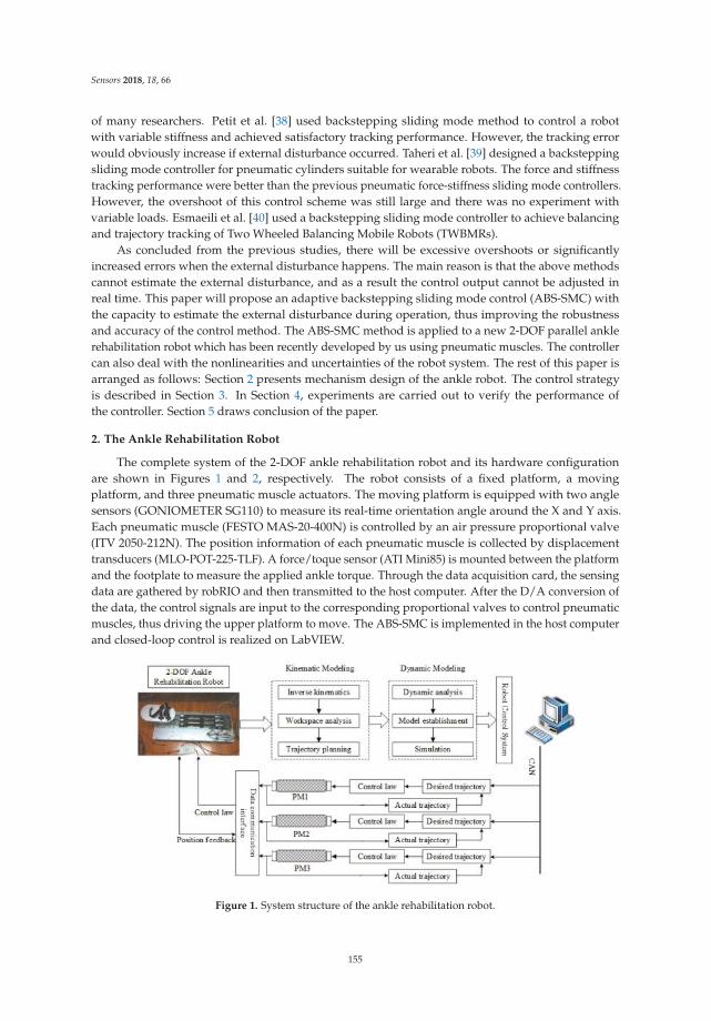
Sensors 2018, 18, 66

of many researchers. Petit et al. [38] used backstepping sliding mode method to control a robotwith variable stiffness and achieved satisfactory tracking performance. However, the tracking errorwould obviously increase if external disturbance occurred. Taheri et al. [39] designed a backsteppingsliding mode controller for pneumatic cylinders suitable for wearable robots. The force and stiffnesstracking performance were better than the previous pneumatic force-stiffness sliding mode controllers.However, the overshoot of this control scheme was still large and there was no experiment withvariable loads. Esmaeili et al. [40] used a backstepping sliding mode controller to achieve balancingand trajectory tracking of Two Wheeled Balancing Mobile Robots (TWBMRs).

As concluded from the previous studies, there will be excessive overshoots or significantlyincreased errors when the external disturbance happens. The main reason is that the above methodscannot estimate the external disturbance, and as a result the control output cannot be adjusted inreal time. This paper will propose an adaptive backstepping sliding mode control (ABS-SMC) withthe capacity to estimate the external disturbance during operation, thus improving the robustnessand accuracy of the control method. The ABS-SMC method is applied to a new 2-DOF parallel anklerehabilitation robot which has been recently developed by us using pneumatic muscles. The controllercan also deal with the nonlinearities and uncertainties of the robot system. The rest of this paper isarranged as follows: Section 2 presents mechanism design of the ankle robot. The control strategyis described in Section 3. In Section 4, experiments are carried out to verify the performance ofthe controller. Section 5 draws conclusion of the paper.

2. The Ankle Rehabilitation Robot

The complete system of the 2-DOF ankle rehabilitation robot and its hardware configurationare shown in Figures 1 and 2, respectively. The robot consists of a fixed platform, a movingplatform, and three pneumatic muscle actuators. The moving platform is equipped with two anglesensors (GONIOMETER SG110) to measure its real-time orientation angle around the X and Y axis.Each pneumatic muscle (FESTO MAS-20-400N) is controlled by an air pressure proportional valve(ITV 2050-212N). The position information of each pneumatic muscle is collected by displacementtransducers (MLO-POT-225-TLF). A force/toque sensor (ATI Mini85) is mounted between the platformand the footplate to measure the applied ankle torque. Through the data acquisition card, the sensingdata are gathered by robRIO and then transmitted to the host computer. After the D/A conversion ofthe data, the control signals are input to the corresponding proportional valves to control pneumaticmuscles, thus driving the upper platform to move. The ABS-SMC is implemented in the host computerand closed-loop control is realized on LabVIEW.

Figure 1. System structure of the ankle rehabilitation robot.

155

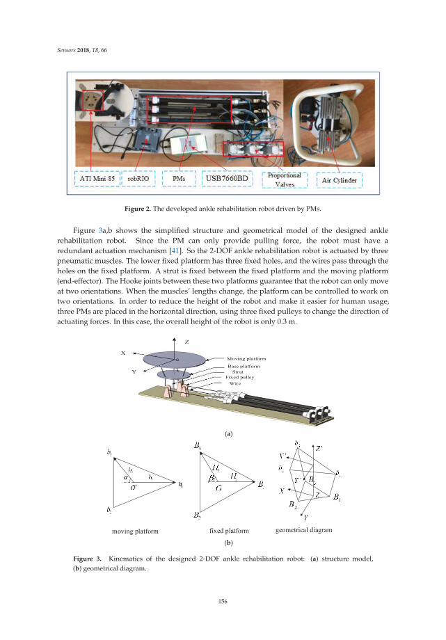
Sensors 2018, 18, 66

Figure 2. The developed ankle rehabilitation robot driven by PMs.

Figure 3a,b shows the simplified structure and geometrical model of the designed anklerehabilitation robot. Since the PM can only provide pulling force, the robot must have aredundant actuation mechanism [41]. So the 2-DOF ankle rehabilitation robot is actuated by threepneumatic muscles. The lower fixed platform has three fixed holes, and the wires pass through theholes on the fixed platform. A strut is fixed between the fixed platform and the moving platform(end-effector). The Hooke joints between these two platforms guarantee that the robot can only moveat two orientations. When the muscles’ lengths change, the platform can be controlled to work ontwo orientations. In order to reduce the height of the robot and make it easier for human usage,three PMs are placed in the horizontal direction, using three fixed pulleys to change the direction ofactuating forces. In this case, the overall height of the robot is only 0.3 m.

(a)

(b)

Figure 3. Kinematics of the designed 2-DOF ankle rehabilitation robot: (a) structure model,(b) geometrical diagram.

156

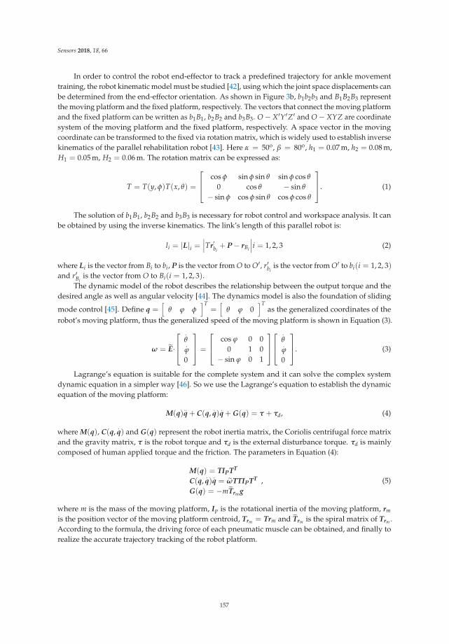
Sensors 2018, 18, 66

In order to control the robot end-effector to track a predefined trajectory for ankle movementtraining, the robot kinematic model must be studied [42], using which the joint space displacements canbe determined from the end-effector orientation. As shown in Figure 3b, b1b2b3 and B1B2B3 representthe moving platform and the fixed platform, respectively. The vectors that connect the moving platformand the fixed platform can be written as b1B1, b2B2 and b3B3. O − X′Y′Z′ and O − XYZ are coordinatesystem of the moving platform and the fixed platform, respectively. A space vector in the movingcoordinate can be transformed to the fixed via rotation matrix, which is widely used to establish inversekinematics of the parallel rehabilitation robot [43]. Here α = 50o, β = 80o, h1 = 0.07 m, h2 = 0.08 m,H1 = 0.05 m, H2 = 0.06 m. The rotation matrix can be expressed as:

T = T(y, φ)T(x, θ) =

⎡⎢⎣

cos φ sin φ sin θ sin φ cos θ

0 cos θ − sin θ

− sin φ cos φ sin θ cos φ cos θ

⎤⎥⎦. (1)

The solution of b1B1, b2B2 and b3B3 is necessary for robot control and workspace analysis. It canbe obtained by using the inverse kinematics. The link’s length of this parallel robot is:

li = |L|i =∣∣∣Tr

′bi+ P − rBi

∣∣∣i = 1, 2, 3 (2)

where Li is the vector from Bi to bi, P is the vector from O to O′, r′biis the vector from O′ to bi(i = 1, 2, 3)

and r′Biis the vector from O to Bi(i = 1, 2, 3).

The dynamic model of the robot describes the relationship between the output torque and thedesired angle as well as angular velocity [44]. The dynamics model is also the foundation of sliding

mode control [45]. Define q =[

θ ϕ φ]T

=[

θ ϕ 0]T

as the generalized coordinates of therobot’s moving platform, thus the generalized speed of the moving platform is shown in Equation (3).

ω = E·

⎡⎢⎣

.θ.ϕ

0

⎤⎥⎦ =

⎡⎢⎣

cos ϕ 0 00 1 0

− sin ϕ 0 1

⎤⎥⎦

⎡⎢⎣

.θ.ϕ

0

⎤⎥⎦. (3)

Lagrange’s equation is suitable for the complete system and it can solve the complex systemdynamic equation in a simpler way [46]. So we use the Lagrange’s equation to establish the dynamicequation of the moving platform:

M(q)..q + C(q,

.q)

.q + G(q) = τ + τd, (4)

where M(q), C(q,.q) and G(q) represent the robot inertia matrix, the Coriolis centrifugal force matrix

and the gravity matrix, τ is the robot torque and τd is the external disturbance torque. τd is mainlycomposed of human applied torque and the friction. The parameters in Equation (4):

M(q) = TIPTT

C(q,.q)

.q = ωTTIPTT

G(q) = −mTrm g

, (5)

where m is the mass of the moving platform, Ip is the rotational inertia of the moving platform, rm

is the position vector of the moving platform centroid, Trm = Trm and Trm is the spiral matrix of Trm .According to the formula, the driving force of each pneumatic muscle can be obtained, and finally torealize the accurate trajectory tracking of the robot platform.

157

Sensors 2018, 18, 66

3. Control Strategy

3.1. Backstepping Sliding Mode Control

The basic idea of backstepping design method is to decompose the complex nonlinear system intosubsystems with lower orders, and then design Lyapunov function and intermediate virtual controlfor each subsystem [47]. Based on Equation (4), the controlled object model can be defined as

{ .q1 = q2.q2 = −M−1Cq2 + M−1τ − M−1G + M−1τd

, (6)

where q1 = q, q is the actual trajectory.Assuming the desired position qd, the controller can be designed by the following two steps:

Step 1: Define the tracking error e1 = q1 − qd, then.e1 =

.q1 −

.qd = q2 −

.qd, and define the Lyapunov

function as

V1 =12

eT1 e1. (7)

So.

V1 = eT1

.e1 = eT

1(q2 −

.qd

). (8)

Defineq2 = e2 +

.qd − c1e1, (9)

where c1 > 0, e2 is a virtual control law. From Equation (9), we can obtain

.e1 =

.q1 −

.qd

= q2 −.qd + c1e − c1e1

= e2 − c1e1

. (10)

From Equations (8) and (10) we can obtain

.V1 = eT

1.e1 = eT

1 e2 − c1eT1 e1. (11)

If e2 = 0,.

V1 = −c1eT1 e1 = −c1(‖e1‖2)

2 ≤ 0. So it is necessary to further design the control law.Step 2: Define the switch function as

s = k1e1 + e2, (12)

where k1 > 0. Taking Equation (10) into (12), we can obtain

s = k1e1 +.e1 + c1e1 = (k1 + c1)e1 +

.e1. (13)

The Lyapunov function is

V2 =12

eT1 e1 +

12

sTs. (14)

From Equation (14) we can obtain

.V2 = eT

1.e1 + sT .

s

= eT1 e2 − c1eT

1 e1 + sT(k1(e2 − c1e1)− M−1C(e2 +.qd − c1e1)

+M−1τ + M−1τd − M−1G − ..qd + c1

.e1)

. (15)

So the control law can be written as

τBS−SMC = τeq + M∆τ, (16)

158

Sensors 2018, 18, 66

whereτeq = M(−k1(e2 − c1e1) + M−1C(e2 +

.qd − c1e1) + M−1G +

..qd − c1

.e1)

∆τ = −h(s + βsgn(s)). (17)

where h and β are the parameters of exponential reaching law. They can determine the speed and timeof the moving point approaching to the sliding surface.

3.2. Adaptive Backstepping Sliding Mode Control

The proposed ABS-SMC can estimate the external disturbance by establishing an disturbanceobserver [48]. Assuming that the external disturbance observer is τd.

Define

Q =

[q1q2

]. (18)

So.

Q =

[ .q1.q2

]=

[q2.q2

]

=

[q2

−M−1Cq2 − M−1G + M−1τ + M−1τd

] , (19)

Equation (19) can be rewritten as:

.Q =

[q2

−M−1Cq2 − M−1G

]+

[0M−1

]τ +

[0M−1

]τd

= f1(Q) + f2(Q)τ + f2(Q)τd

, (20)

where

f1(Q) =

[q2

−M−1Cq2 − M−1G

]; f2(Q) =

[0M−1

], (21)

The disturbance observer is designed based on the difference between estimated output andactual output. Equation (20) can be rewritten as

f2(Q)τd =.

Q − f1(Q)− f2(Q)τ, (22)

So the disturbance observer is designed:

.τd = Γ(

.Q − f1(Q)− f2(Q)τ − f2(Q)τd), (23)

Define vector z = τd − p(Q). The observer gain can be expressed as Γ = ∂p(Q)/∂Q. Let

Γ =[

ξ2 ξ2

],ξ1 > 0, ξ2 > 0 (24)

p(Q) = ξ1q1 + ξ2q2 = ξ1q + ξ2.q. (25)

.z =

.τd −

.p(Q). (26)

Substituting Equations (23) and (25) into (26),

.z =

.τd −

.p(Q)

= Γ(− f1(Q)− f2(Q)τ − f2(Q)(z + p(Q)))

+[

ξ1 ξ2

][.q

..q

]T− ξ1

.q − ξ2

..q

= Γ(− f1(Q)− f2(Q)τ − f2(Q)(z + p(Q)))

. (27)

159

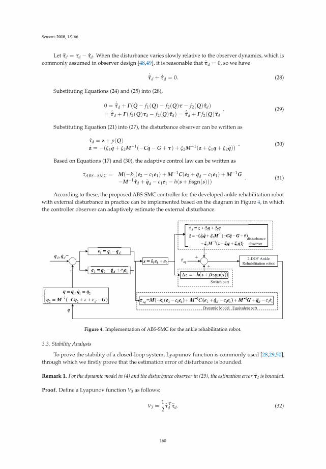
Sensors 2018, 18, 66

Let τd = τd − τd. When the disturbance varies slowly relative to the observer dynamics, which iscommonly assumed in observer design [48,49], it is reasonable that

.τd = 0, so we have

.

τd +.τd = 0. (28)

Substituting Equations (24) and (25) into (28),

0 =.

τd + Γ(.

Q − f1(Q)− f2(Q)τ − f2(Q)τd)

=.

τd + Γ( f2(Q)τd − f2(Q)τd) =.

τd + Γ f2(Q)τd

. (29)

Substituting Equation (21) into (27), the disturbance observer can be written as

τd = z + p(Q).z = −(ξ1

.q + ξ2M−1(−C

.q − G + τ) + ξ2M−1(z + ξ1q + ξ2

.q))

. (30)

Based on Equations (17) and (30), the adaptive control law can be written as

τABS−SMC = M(−k1(e2 − c1e1) + M−1C(e2 +.qd − c1e1) + M−1G

−M−1τd +..qd − c1

.e1 − h(s + βsgn(s)))

. (31)

According to these, the proposed ABS-SMC controller for the developed ankle rehabilitation robotwith external disturbance in practice can be implemented based on the diagram in Figure 4, in whichthe controller observer can adaptively estimate the external disturbance.

Switch part

Dynamic Model Equivalent partDynayyyy mic Model Equiqqqq valent pppppart

disturbance observer

2-DOF Ankle Rehabilitation robot

d

Figure 4. Implementation of ABS-SMC for the ankle rehabilitation robot.

3.3. Stability Analysis

To prove the stability of a closed-loop system, Lyapunov function is commonly used [28,29,50],through which we firstly prove that the estimation error of disturbance is bounded.

Remark 1. For the dynamic model in (4) and the disturbance observer in (29), the estimation error τd is bounded.

Proof. Define a Lyapunov function V3 as follows:

V3 =12

τTd τd. (32)

160

Sensors 2018, 18, 66

Substituting Equations (21) and (24) into (23):

.τd =

[ξ1 ξ2

]([ .q1.q2

]−

[q2−M−1Cq2 − M−1G

]−

[0M−1

]τ −

[0M−1

]τd

)

= ξ2(..q + M−1Cq2 + M−1G − M−1τ − M−1τd)

. (33)

Substituting Equation (6) into (33):

.τd = ξ2(M

−1τd − M−1τd) = ξ2M−1τd. (34)

So

τTd

.

τd = τTd (

.τd −

.τd) = −τT

d

.τd. (35)

Substituting Equation (34) into (35), we have

τTd

.

τd = −ξ2τTd M−1τd. (36)

Because M−1 is a positive definite matrix and ξ2 > 0, then

.V3 = τT

d

.

τd ≤ 0. (37)

This indicates that the designed disturbance observer can track external disturbance, which meansthe estimation error τd is bounded, so Remark 1 is proved to be correct.

Then, we prove the stability of the combined system. As the robot moves within a confined space,the inertia matrix M is bounded and positive definite so M−1 exists and is bounded,

‖M−1τd‖1 = ‖M−1τd − M−1τd‖1 ≤ δ. (38)

δ is the estimated value of δ. Then define:.δ = γ‖s‖1. (39)

where γ > 0 [51,52]. �

Remark 2. As long as the parameters are appropriately set, the closed-loop system is stable for disturbance

observer in (30) and control law in (31).

Proof. The Lyapunov function is defined as

V = V2 +1

2γδ2 +

12

τTd τd. (40)

where δ = δ − δ.From Equation (40), we can get

.V =

.V2 +

1γ

δ.

δ + τTd

.

τd. (41)

Substituting Equation (31) into (15), we can get

.V2 +

1γ δ

.

δ = eT1 e2 − c1eT

1 e1 + sTM−1τd − hsTs − hβ‖s‖1 − 1γ δ

.δ

≤ eT1 e2 − c1eT

1 e1 + δ‖s‖1 − hsTs − hβ‖s‖1 − δ‖s‖1= eT

1 e2 − c1eT1 e1 − hsTs + (δ − δ − hβ)‖s‖1

. (42)

161

Sensors 2018, 18, 66

Let hβ = δ =∫

γ‖s‖1dt. Equation (42) can be rewritten as:

.V2 +

1γ δ

.

δ ≤ eT1 e2 − c1eT

1 e1 − hsTs + (δ − δ − hβ)‖s‖1

= eT1 e2 − c1eT

1 e1 − hsTs + (δ − δ − δ)‖s‖1= eT

1 e2 − c1eT1 e1 − hsTs

. (43)

Define e =[

eT1 eT

2

], eT =

[e1

e2

], and =

[c1 + hk2

1 hk1 − 12

hk1 − 12 h

].

Then

eBeT =[

eT1 eT

2

][ c1 + hk21 hk1 − 1

2hk1 − 1

2 h

][e1

e2

]

= c1eT1 e1 − eT

1 e2 + hk21eT

1 e1 + hk1eT1 e2 + hk1eT

2 e1 + heT2 e2

= c1eT1 e1 − eT

1 e2 + hsTs

. (44)

Substituting Equation (44) into (43):

.V2 +

1γ

δ.

δ ≤ −eBeT . (45)

If we make be a positive definite matrix, then

.V2 +

1γ

δ.

δ ≤ −eTBe ≤ 0. (46)

Because|B| = h(c1 + hk2

1)− (hk1 − 12 )

2

= h(c1 + k1)− 14

. (47)

By appropriately setting h, c1, k1, we can make |B| > 0, so that B is a positive definite matrix and

guarantee.

V2 +1γ δ

.

δ ≤ 0.From Equation (37), we can get

τTd

.

τd ≤ 0. (48)

Substituting Equations (46) and (48) into (41):

.V =

.V2 +

1γ

δ.

δ + τTd

.

τd ≤ 0. (49)

Therefore, as long as the mentioned parameters are appropriately set, we can ensure the systembe stable. In this way, Remark 2 is proved to be correct. �

4. Experimental and Results Discussion

In order to confirm the performance of the proposed control method, experiments were carriedout on the 2-DOF ankle rehabilitation robot. The experiments can be divided into four groups: (1) stepresponse experiment; (2) sine trajectory tracking experiment (without subject); (3) robustness test withhuman subjects; and (4) sudden external disturbance experiment. BS-SMC has been widely usedin recent years and achieved good control performance [38–40], so we conduct the experiments tocompare the proposed control method with BS-SMC to verify its control capacity and advantages.

162

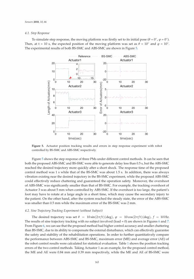
Sensors 2018, 18, 66

4.1. Step Response

To simulate step response, the moving platform was firstly set to its initial pose (θ = 0◦, ϕ = 0◦).Then, at t = 10 s, the expected position of the moving platform was set as θ = 10◦ and ϕ = 10◦.The experimental results of both BS-SMC and ABS-SMC are shown in Figure 5.

0 10 20 300

10

20Actuator1

Reference BS-SMC ABS-SMC

0 10 20 30

6

8

10

Length

of A

ctu

ato

rs(m

m)

Actuator2

0 10 20 300

20

40

time(sec)

Actuator3

0 10 20 30-20

0

20Actuator1

0 10 20 30-5

0

5

Err

or

of A

ctu

ato

rs(m

m)

Actuator2

0 10 20 30-20

0

20

time(sec)

Actuator3

10 15

0

2

4

Figure 5. Actuator position tracking results and errors in step response experiment with robotcontrolled by BS-SMC and ABS-SMC respectively.

Figure 5 shows the step response of three PMs under different control methods. It can be seen thatboth the proposed ABS-SMC and BS-SMC were able to generate delay less than 0.5 s, but the ABS-SMCreached the desired trajectory more quickly after a short shock. The response time of the proposedcontrol method was 1 s while that of the BS-SMC was about 1.5 s. In addition, there was alwaysvibration existing near the desired trajectory in the BS-SMC experiment, while the proposed ABS-SMCcould effectively reduce chattering and guaranteed the operation safety. Moreover, the overshootof ABS-SMC was significantly smaller than that of BS-SMC. For example, the tracking overshoot ofActuator 3 was about 5 mm when controlled by ABS-SMC. If the overshoot is too large, the patient’sfoot may have to rotate at a large angle in a short time, which may cause the secondary injury tothe patient. On the other hand, after the system reached the steady state, the error of the ABS-SMCwas smaller than 0.5 mm while the maximum error of the BS-SMC was 2 mm.

4.2. Sine Trajectory Tracking Experiment (without Subject)

The desired trajectory was set θ = 10 sin(2π f t)(deg), ϕ = 10 cos(2π f t)(deg), f = 10 Hz.The results of sine trajectory tracking with no subject involved (load = 0) are shown in Figures 6 and 7.From Figure 6, we can see that the proposed method had higher control accuracy and smaller chatteringthan BS-SMC, due to its ability to compensate the external disturbance, which can effectively guaranteethe safety and stability of the rehabilitation operations. In order to further quantitatively comparethe performance between ABS-SMC and BS-SMC, maximum error (ME) and average error (AE) ofthe robot control results were calculated for statistical evaluation. Table 1 shows the position trackingerrors of the two control methods. Taking Actuator 1 as an example, for the proposed control method,the ME and AE were 0.84 mm and 0.39 mm respectively, while the ME and AE of BS-SMC were

163

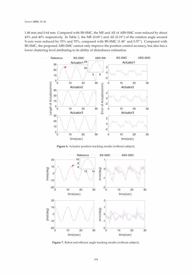
Sensors 2018, 18, 66

1.48 mm and 0.64 mm. Compared with BS-SMC, the ME and AE of ABS-SMC were reduced by about43% and 40% respectively. In Table 2, the ME (0.69◦) and AE (0.19◦) of the rotation angle aroundX-axis were reduced by 53% and 70%, compared with BS-SMC (1.48◦ and 0.57◦). Compared withBS-SMC, the proposed ABS-SMC cannot only improve the position control accuracy, but also has alower chattering level attributing to its ability of disturbance estimation.

0 10 20 300

10

20

30Actuator1

Reference BS-SMC ABS-SMC

0 10 20 300

10

20

30

Length

of A

ctu

ato

rs(m

m)

Actuator2

0 10 20 300

10

20

30

time(sec)

Actuator3

0 10 20 30

-2

0

2

Actuator1

BS-SMC ABS-SMC

0 10 20 30

-2

0

2

Err

or

of A

ctu

ato

rs(m

m)

Actuator2

0 10 20 30

-2

0

2

time(sec)

Actuator3

4 6

20

25

Figure 6. Actuator position tracking results (without subject).

0 10 20 30-20

-10

0

10

20

time(sec)

theta

(deg)

Reference BS-SMC ABS-SMC

0 10 20 30-20

-10

0

10

20

time(sec)

phai(deg)

0 10 20 30-2

-1

0

1

time(sec)

err

or(

deg)

0 10 20 30-2

-1

0

1

2

time(sec)

err

or(

deg)

12 14

6

8

10

Figure 7. Robot end-effector angle tracking results (without subject).

164

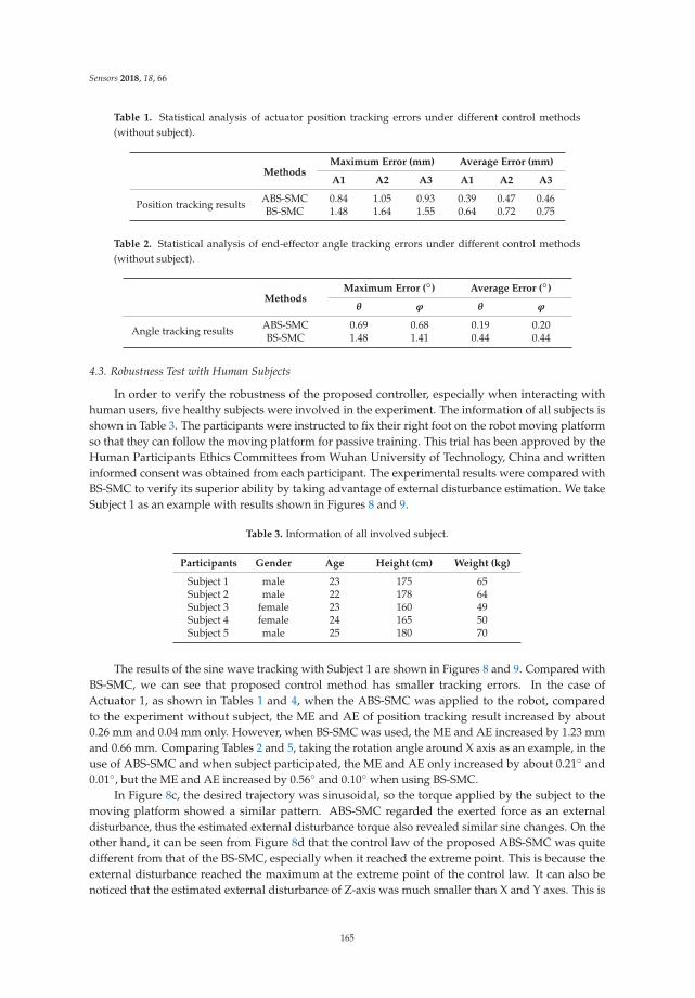
Sensors 2018, 18, 66

Table 1. Statistical analysis of actuator position tracking errors under different control methods(without subject).

MethodsMaximum Error (mm) Average Error (mm)

A1 A2 A3 A1 A2 A3

Position tracking results ABS-SMC 0.84 1.05 0.93 0.39 0.47 0.46BS-SMC 1.48 1.64 1.55 0.64 0.72 0.75

Table 2. Statistical analysis of end-effector angle tracking errors under different control methods(without subject).

MethodsMaximum Error (◦) Average Error (◦)

θ ϕ θ ϕ

Angle tracking results ABS-SMC 0.69 0.68 0.19 0.20BS-SMC 1.48 1.41 0.44 0.44

4.3. Robustness Test with Human Subjects

In order to verify the robustness of the proposed controller, especially when interacting withhuman users, five healthy subjects were involved in the experiment. The information of all subjects isshown in Table 3. The participants were instructed to fix their right foot on the robot moving platformso that they can follow the moving platform for passive training. This trial has been approved by theHuman Participants Ethics Committees from Wuhan University of Technology, China and writteninformed consent was obtained from each participant. The experimental results were compared withBS-SMC to verify its superior ability by taking advantage of external disturbance estimation. We takeSubject 1 as an example with results shown in Figures 8 and 9.

Table 3. Information of all involved subject.

Participants Gender Age Height (cm) Weight (kg)

Subject 1 male 23 175 65Subject 2 male 22 178 64Subject 3 female 23 160 49Subject 4 female 24 165 50Subject 5 male 25 180 70

The results of the sine wave tracking with Subject 1 are shown in Figures 8 and 9. Compared withBS-SMC, we can see that proposed control method has smaller tracking errors. In the case ofActuator 1, as shown in Tables 1 and 4, when the ABS-SMC was applied to the robot, comparedto the experiment without subject, the ME and AE of position tracking result increased by about0.26 mm and 0.04 mm only. However, when BS-SMC was used, the ME and AE increased by 1.23 mmand 0.66 mm. Comparing Tables 2 and 5, taking the rotation angle around X axis as an example, in theuse of ABS-SMC and when subject participated, the ME and AE only increased by about 0.21◦ and0.01◦, but the ME and AE increased by 0.56◦ and 0.10◦ when using BS-SMC.

In Figure 8c, the desired trajectory was sinusoidal, so the torque applied by the subject to themoving platform showed a similar pattern. ABS-SMC regarded the exerted force as an externaldisturbance, thus the estimated external disturbance torque also revealed similar sine changes. On theother hand, it can be seen from Figure 8d that the control law of the proposed ABS-SMC was quitedifferent from that of the BS-SMC, especially when it reached the extreme point. This is because theexternal disturbance reached the maximum at the extreme point of the control law. It can also benoticed that the estimated external disturbance of Z-axis was much smaller than X and Y axes. This is

165

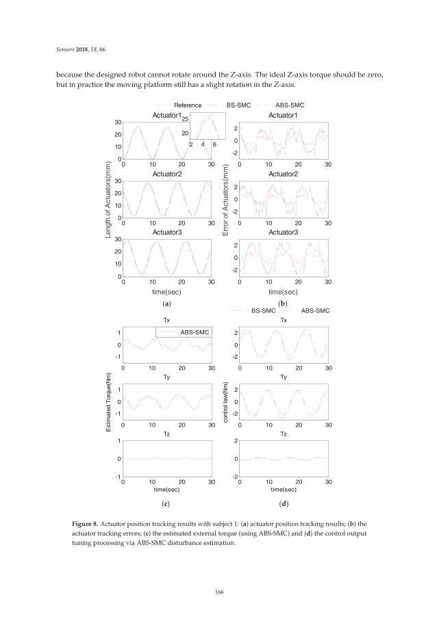
Sensors 2018, 18, 66

because the designed robot cannot rotate around the Z-axis. The ideal Z-axis torque should be zero,but in practice the moving platform still has a slight rotation in the Z-axis.

(a) (b)

(c) (d)

0 10 20 300

10

20

30Actuator1

Reference BS-SMC ABS-SMC

0 10 20 300

10

20

30

Length

of A

ctu

ato

rs(m

m)

Actuator2

0 10 20 300

10

20

30

time(sec)

Actuator3

0 10 20 30

-2

0

2

Actuator1

0 10 20 30

-2

0

2

Err

or

of A

ctu

ato

rs(m

m)

Actuator2

0 10 20 30

-2

0

2

time(sec)

Actuator3

2 4 6

20

25

0 10 20 30

-1

0

1

Tx

ABS-SMC

0 10 20 30

-1

0

1

Estim

ate

d T

orq

ue(N

m)

Ty

0 10 20 30-1

0

1

time(sec)

Tz

0 10 20 30

-2

0

2

Tx

BS-SMC ABS-SMC

0 10 20 30

-2

0

2

contr

ol la

w(N

m)

Ty

0 10 20 30-2

0

2

time(sec)

Tz

Figure 8. Actuator position tracking results with subject 1: (a) actuator position tracking results; (b) theactuator tracking errors; (c) the estimated external torque (using ABS-SMC) and (d) the control outputtuning processing via ABS-SMC disturbance estimation.

166

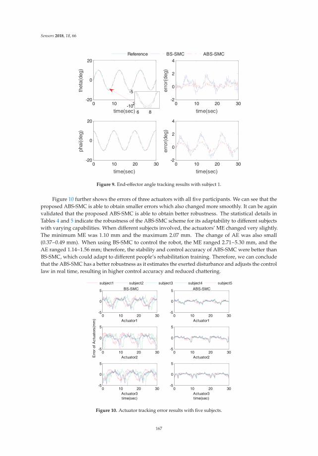
Sensors 2018, 18, 66

0 10 20 30-20

0

20

time(sec)

theta

(deg)

Reference BS-SMC ABS-SMC

0 10 20 30-20

0

20

time(sec)

phai(deg)

0 10 20 30-2

0

2

4

time(sec)

err

or(

deg)

0 10 20 30-2

0

2

4

time(sec)

err

or(

deg)

6 8

-10

-5

Figure 9. End-effector angle tracking results with subject 1.

Figure 10 further shows the errors of three actuators with all five participants. We can see that theproposed ABS-SMC is able to obtain smaller errors which also changed more smoothly. It can be againvalidated that the proposed ABS-SMC is able to obtain better robustness. The statistical details inTables 4 and 5 indicate the robustness of the ABS-SMC scheme for its adaptability to different subjectswith varying capabilities. When different subjects involved, the actuators’ ME changed very slightly.The minimum ME was 1.10 mm and the maximum 2.07 mm. The change of AE was also small(0.37~0.49 mm). When using BS-SMC to control the robot, the ME ranged 2.71~5.30 mm, and theAE ranged 1.14~1.56 mm; therefore, the stability and control accuracy of ABS-SMC were better thanBS-SMC, which could adapt to different people’s rehabilitation training. Therefore, we can concludethat the ABS-SMC has a better robustness as it estimates the exerted disturbance and adjusts the controllaw in real time, resulting in higher control accuracy and reduced chattering.

0 10 20 30-5

0

5

Actuator1

ABS-SMC

subject1 subject2 subject3 subject4 subject5

0 10 20 30-5

0

5

Actuator2

0 10 20 30-5

0

5

Actuator3

time(sec)

0 10 20 30-5

0

5

Actuator1

BS-SMC

0 10 20 30-5

0

5

Err

or

of

Actu

ato

rs(m

m)

Actuator2

0 10 20 30-5

0

5

Actuator3

time(sec)

Figure 10. Actuator tracking error results with five subjects.

167

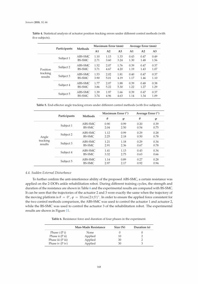
Sensors 2018, 18, 66

Table 4. Statistical analysis of actuator position tracking errors under different control methods (withfive subjects).

Participants MethodsMaximum Error (mm) Average Error (mm)

A1 A2 A3 A1 A2 A3

Positiontrackingresults

Subject 1 ABS-SMC 1.10 1.13 1.33 0.43 0.47 0.49BS-SMC 2.71 3.60 3.24 1.30 1.48 1.56

Subject 2 ABS-SMC 1.52 2.07 1.76 0.39 0.47 0.37BS-SMC 3.71 4.67 4.20 1.19 1.43 1.07

Subject 3 ABS-SMC 1.53 2.02 1.81 0.40 0.47 0.37BS-SMC 3.90 5.01 4.19 1.17 1.46 1.10

Subject 4 ABS-SMC 1.77 2.07 1.88 0.39 0.48 0.38BS-SMC 3.86 5.22 5.30 1.22 1.27 1.29

Subject 5 ABS-SMC 1.39 1.97 1.66 0.39 0.47 0.37BS-SMC 3.74 4.96 4.63 1.14 1.34 1.09

Table 5. End-effector angle tracking errors under different control methods (with five subjects).

Participants MethodsMaximum Error (◦) Average Error (◦)

θ ϕ θ ϕ

Angletrackingresults

Subject 1 ABS-SMC 0.90 0.99 0.20 0.39BS-SMC 2.04 2.50 0.54 0.75

Subject 2 ABS-SMC 1.12 0.99 0.29 0.28BS-SMC 2.25 2.18 0.50 0.78

Subject 3 ABS-SMC 1.21 1.18 0.29 0.34BS-SMC 2.91 2.36 0.67 0.78

Subject 4 ABS-SMC 1.41 1.13 0.43 0.34BS-SMC 3.32 2.75 0.63 0.66

Subject 5 ABS-SMC 1.14 0.89 0.27 0.28BS-SMC 2.97 2.17 0.92 0.94

4.4. Sudden External Disturbance

To further confirm the anti-interference ability of the proposed ABS-SMC, a certain resistance wasapplied on the 2-DOFs ankle rehabilitation robot. During different training cycles, the strength andduration of the resistance are shown in Table 6 and the experimental results are compared with BS-SMC.It can be seen that the trajectories of the actuator 2 and 3 were exactly the same when the trajectory ofthe moving platform is θ = 0◦, ϕ = 10 cos(2π f t)◦. In order to ensure the applied force consistent forthe two control methods comparison, the ABS-SMC was used to control the actuator 1 and actuator 2,while the BS-SMC was used to control the actuator 3 of the rehabilitation robot. The experimentalresults are shown in Figure 11.

Table 6. Resistance force and duration of four phases in the experiment.

Man-Made Resistance Size (N) Duration (s)

Phase i (P i) None 0 0Phase ii (P ii) Applied 10 2

Phase iii (P iii) Applied 30 2Phase iv (P iv) Applied 30 3

168

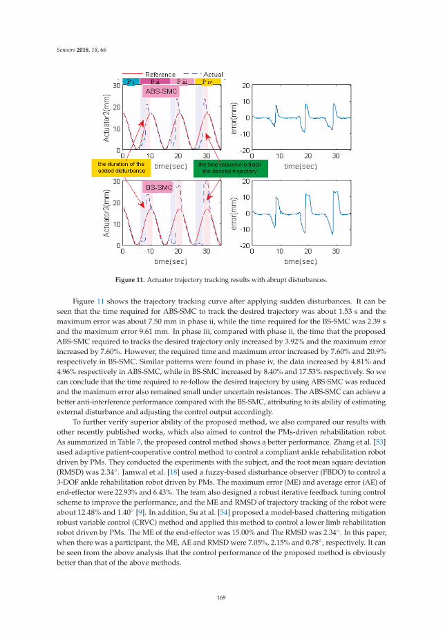
Sensors 2018, 18, 66

Figure 11. Actuator trajectory tracking results with abrupt disturbances.

Figure 11 shows the trajectory tracking curve after applying sudden disturbances. It can beseen that the time required for ABS-SMC to track the desired trajectory was about 1.53 s and themaximum error was about 7.50 mm in phase ii, while the time required for the BS-SMC was 2.39 sand the maximum error 9.61 mm. In phase iii, compared with phase ii, the time that the proposedABS-SMC required to tracks the desired trajectory only increased by 3.92% and the maximum errorincreased by 7.60%. However, the required time and maximum error increased by 7.60% and 20.9%respectively in BS-SMC. Similar patterns were found in phase iv, the data increased by 4.81% and4.96% respectively in ABS-SMC, while in BS-SMC increased by 8.40% and 17.53% respectively. So wecan conclude that the time required to re-follow the desired trajectory by using ABS-SMC was reducedand the maximum error also remained small under uncertain resistances. The ABS-SMC can achieve abetter anti-interference performance compared with the BS-SMC, attributing to its ability of estimatingexternal disturbance and adjusting the control output accordingly.

To further verify superior ability of the proposed method, we also compared our results withother recently published works, which also aimed to control the PMs-driven rehabilitation robot.As summarized in Table 7, the proposed control method shows a better performance. Zhang et al. [53]used adaptive patient-cooperative control method to control a compliant ankle rehabilitation robotdriven by PMs. They conducted the experiments with the subject, and the root mean square deviation(RMSD) was 2.34◦. Jamwal et al. [18] used a fuzzy-based disturbance observer (FBDO) to control a3-DOF ankle rehabilitation robot driven by PMs. The maximum error (ME) and average error (AE) ofend-effector were 22.93% and 6.43%. The team also designed a robust iterative feedback tuning controlscheme to improve the performance, and the ME and RMSD of trajectory tracking of the robot wereabout 12.48% and 1.40◦ [9]. In addition, Su at al. [54] proposed a model-based chattering mitigationrobust variable control (CRVC) method and applied this method to control a lower limb rehabilitationrobot driven by PMs. The ME of the end-effector was 15.00% and The RMSD was 2.34◦. In this paper,when there was a participant, the ME, AE and RMSD were 7.05%, 2.15% and 0.78◦, respectively. It canbe seen from the above analysis that the control performance of the proposed method is obviouslybetter than that of the above methods.

169

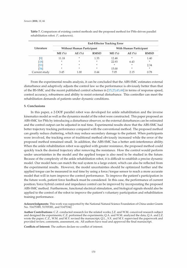
Sensors 2018, 18, 66

Table 7. Comparison of existing control methods and the proposed method for PMs-driven parallelrehabilitation robot. (*, unknown).

Literature

End-Effector Tracking Error

Without Human Participant With Human Participant

ME (%) AE (%) RMSD ME (%) AE (%) RMSD

[9] 11.18 * 1.35 12.48 * 1.40[18] * * * 22.93 6.43 *[53] * * * * * 2.34[54] * * * 15.00 * *

Current study 3.45 1.00 0.44 7.05 2.15 0.78

From the experimental results analysis, it can be concluded that the ABS-SMC estimates externaldisturbance and adaptively adjusts the control law so the performance is obviously better than thatof the BS-SMC and the recent published control schemes in [15,23,43,44] in terms of response speed,control accuracy, robustness and ability to resist external disturbance. This controller can meet therehabilitation demands of patients under dynamic conditions.

5. Conclusions

In this paper, a 2-DOF parallel robot was developed for ankle rehabilitation and the inversekinematics model as well as the dynamics model of the robot were constructed. This paper proposed anABS-SMC for PMs by introducing a disturbance observer, so the external disturbances can be estimatedand the control output can be adjusted in real time. Experimental results show that the ABS-SMC hadbetter trajectory tracking performance compared with the conventional method. The proposed methodcan greatly reduce chattering, which may reduce secondary damage to the patient. When participantswere involved, the tracking error of traditional method obviously increased while the error of theproposed method remained small. In addition, the ABS-SMC has a better anti-interference ability.When the ankle rehabilitation robot was applied with greater resistance, the proposed method couldquickly track the desired trajectory after removing the resistance. How the control would performunder uncertainties in the model and the applied torque is also need to be studied in the future.Because of the complexity of the ankle rehabilitation robot, it is difficult to establish a precise dynamicmodel. Our model here can match the real system to a large extent, which can also be reflected fromthe experimental results. However, the model uncertainties should be optimized further and theapplied torque can be measured in real time by using a force/torque sensor to reach a more accuratemodel that will in turn improve the control performance. To improve the patient’s participation inthe future work, patient force feedback must be considered. In this case, the performance of currentposition/force hybrid control and impedance control can be improved by incorporating the proposedABS-SMC method. Furthermore, functional electrical stimulation, and biological signals should also beapplied to the control of the robot to improve the patient’s voluntary participation and rehabilitationtraining performance.

Acknowledgments: This work was supported by the National Natural Science Foundation of China under GrantsNo. 51675389, 51705381, and 51475342.

Author Contributions: C.Z. conducted research for the related works; J.Z. and W.M. conceived research subjectand designed the experiments; C.Z. performed the experiments; Q.A. and W.M. analyzed the data; Q.A. and J.Z.wrote the paper; C.Z., W.M. and M.Y. revised the manuscript; Q.L., S.X. and M.Y. supervised the paperwork andprovided review, comments, assessment, etc. All authors have read and approved the final manuscript.

Conflicts of Interest: The authors declare no conflict of interest.

170

Sensors 2018, 18, 66

References

1. Zhang, M.; Davies, T.C.; Xie, S. Effectiveness of robot-assisted therapy on ankle rehabilitation—A systematicreview. J. Neuroeng. Rehabil. 2013, 10, 30. [CrossRef] [PubMed]

2. Staniszewski, M.; Zybko, P.; Wiszomirska, I. Influence of a nine-day alpine ski training programme on thepostural stability of people with different levels of skills. Biomed. Hum. Kinet. 2016, 8, 24–31. [CrossRef]

3. Omar, S.M.M.H.; El-Kalaa, F.A.; Ali, E.S.F.; El-Karim, A.A.A.; Sekily, N.M.E. Anatomical and magneticresonance imaging study of the medial collateral ligament of the ankle joint. Alex. J. Med. 2016, 52, 73–81.[CrossRef]

4. Hertel, J. Functional anatomy, pathomechanics, and pathophysiology of lateral ankle instability. J. Athl. Train.

2002, 37, 364. [PubMed]5. Farulla, G.A.; Pianu, D.; Cempini, M.; Cortese, M.; Russo, L.O.; Indaco, M.; Nerino, R.; Chimienti, A.;

Oddo, C.M.; Vitiello, N. Vision-based pose estimation for robot-mediated hand telerehabilitation. Sensors

2016, 16, 208. [CrossRef] [PubMed]6. Saadat, M.; Rastegarpanah, A.; Abdullah, C.Z.; Rakhodaei, H.; Borboni, A.; Maddalena, M. Path’s slicing

analysis as a therapist’s intervention tool for robotic rehabilitation. In Advances in Service and Industrial

Robotics, Proceedings of the 26th International Conference on Robotics in Alpe-Adria-Danube Region (RAAD 2017),

Turin, Italy, 21–23 June 2017; Ferraresi, C., Quaglia, G., Eds.; Springer International Publishing: Cham,Switzerland, 2018; pp. 901–910.

7. Borboni, A.; Maddalena, M.; Rastegarpanah, A.; Saadat, M.; Aggogeri, F. Kinematic performanceenhancement of wheelchair-mounted robotic arm by adding a linear drive. In Proceedings of the IEEEInternational Symposium on Medical Measurements and Applications, Benevento, Italy, 15–18 May 2016;pp. 1–6.

8. Ai, Q.; Liu, Q.; Yuan, T.; Lu, Y. Gestures recognition based on wavelet and LLE. Australas. Phys. Eng. Sci. Med.

2013, 36, 167–176. [CrossRef] [PubMed]9. Meng, W.; Xie, S.Q.; Liu, Q.; Lu, C.Z.; Ai, Q. Robust iterative feedback tuning control of a compliant

rehabilitation robot for repetitive ankle training. IEEE/ASME Trans. Mechatron. 2017, 22, 173–184. [CrossRef]10. Meng, W.; Liu, Q.; Zhou, Z.; Ai, Q.; Sheng, B.; Xie, S.S. Recent development of mechanisms and control

strategies for robot-assisted lower limb rehabilitation. Mechatronics 2015, 31, 132–145. [CrossRef]11. Liu, Q.; Liu, D.; Meng, W.; Zhou, Z.; Ai, Q. Fuzzy sliding mode control of a multi-DOF parallel robot in

rehabilitation environment. Int. J. Humanoid Robot. 2014, 11, 1450004. [CrossRef]12. Rastegarpanah, A.; Saadat, M.; Borboni, A. Parallel robot for lower limb rehabilitation exercises.

Appl. Bionics Biomech. 2016, 2016. [CrossRef] [PubMed]13. Rastegarpanah, A.; Saadat, M.; Borboni, A.; Stolkin, R. Application of a parallel robot in lower limb

rehabilitation: A brief capability study. In Proceedings of the 1st International Conference on Robotics andAutomation for Humanitarian Applications (RAHA 2016), Kerala, India, 18–20 December 2016.

14. Pehlivan, A.U.; Sergi, F.; O’Malley, M.K. A subject-adaptive controller for wrist robotic rehabilitation.IEEE/ASME Trans. Mechatron. 2015, 20, 1338–1350. [CrossRef]

15. Repperger, D.W.; Phillips, C.A.; Neidhard-Doll, A.; Reynolds, D.B.; Berlin, J. Actuator design usingbiomimicry methods and a pneumatic muscle system. Control Eng. Pract. 2006, 14, 999–1009. [CrossRef]

16. Ba, D.X.; Ahn, K.K. Indirect sliding mode control based on gray-box identification method for pneumaticartificial muscle. Mechatronics 2015, 32, 1–11. [CrossRef]

17. Xie, S.Q.; Jamwal, P.K. An iterative fuzzy controller for pneumatic muscle driven rehabilitation robot.Expert Syst. Appl. 2011, 38, 8128–8137. [CrossRef]

18. Jamwal, P.K.; Xie, S.Q.; Hussain, S.; Parsons, J.G. An adaptive wearable parallel robot for the treatment ofankle injuries. IEEE/ASME Trans. Mechatron. 2014, 19, 64–75. [CrossRef]

19. Park, Y.-L.; Chen, B.-R.; Young, D.; Stirling, L.; Wood, R.J.; Goldfield, E.; Nagpal, R. Bio-inspired active softorthotic device for ankle foot pathologies. In Proceedings of the 2011 IEEE/RSJ International Conferenceon Intelligent Robots and Systems: Celebrating 50 Years of Robotics (IROS’11), San Francisco, CA, USA,25–30 September 2011; Institute of Electrical and Electronics Engineers Inc.: San Francisco, CA, USA;pp. 4488–4495.

20. Sawicki, G.S.; Ferris, D.P. A pneumatically powered knee-ankle-foot orthosis (kafo) with myoelectricactivation and inhibition. J. Neuroeng. Rehabil. 2009, 6, 23. [CrossRef] [PubMed]

171

Sensors 2018, 18, 66

21. Murphy, P.; Adolf, G.; Daly, S.; Bolton, M.; Maurice, O.; Bonia, T.; Mavroidis, C.; Yen, S.-C. Test of a customizedcompliant ankle rehabilitation device in unpowered mode. In Proceedings of the 36th Annual InternationalConference of the IEEE Engineering in Medicine and Biology Society, Chicago, IL, USA, 26–30 August 2014;Volume 2014, pp. 3057–3060.

22. Lin, L.-H.; Yen, J.-Y.; Wang, F.-C. System identification and robust control of a pneumatic muscleactuator system. In Proceedings of the 2nd International Conference on Engineering and TechnologyInnovation 2012 (ICETI 2012), Kaohsiung, Taiwan, 2–6 November 2012; Trans Tech Publications:Kaohsiung, Taiwan, 2013; pp. 1936–1940.

23. Chang, M.-K.; Liou, J.-J.; Chen, M.-L. T-s fuzzy model-based tracking control of a one-dimensionalmanipulator actuated by pneumatic artificial muscles. Control Eng. Pract. 2011, 19, 1442–1449. [CrossRef]

24. Zhao, J.; Zhong, J.; Fan, J. Position control of a pneumatic muscle actuator using RBF neural network tunedPID controller. Math. Prob. Eng. 2015, 2015. [CrossRef]

25. Zhang, J.-F.; Yang, C.-J.; Chen, Y.; Zhang, Y.; Dong, Y.-M. Modeling and control of a curved pneumatic muscleactuator for wearable elbow exoskeleton. Mechatronics 2008, 18, 448–457. [CrossRef]

26. Choi, T.-Y.; Choi, B.-S.; Seo, K.-H. Position and compliance control of a pneumatic muscle actuatedmanipulator for enhanced safety. IEEE Trans. Control Syst. Technol. 2011, 19, 832–842. [CrossRef]

27. Jiang, F.; Tao, G.; Li, Q. Analysis and control of a parallel lower limb based on pneumatic artificial muscles.Adv. Mech. Eng. 2016, 9, 1–14. [CrossRef]

28. Fan, Q.Y.; Yang, G.H. Adaptive actor-critic design-based integral sliding-mode control for partially unknownnonlinear systems with input disturbances. IEEE Trans. Neural Netw. Learn. Syst. 2016, 27, 165–177.[CrossRef] [PubMed]

29. Liu, S.Y.; Liu, Y.C.; Wang, N. Nonlinear disturbance observer-based backstepping finite-time sliding modetracking control of underwater vehicles with system uncertainties and external disturbances. Nonlinear Dyn.

2017, 88, 465–476. [CrossRef]30. Mohammadi, A.; Tavakoli, M.; Marquez, H.J.; Hashemzadeh, F. Nonlinear disturbance observer design for

robotic manipulators. Control Eng. Pract. 2013, 21, 253–267. [CrossRef]31. Yang, H.J.; Yu, Y.; Qiu, J.; Hua, C.C. Active disturbance rejection tracking control for a nonlinear pneumatic

muscle system. Int. J. Control Autom. Syst. 2017, 15, 2376–2384. [CrossRef]32. Zhu, X.C.; Tao, G.L.; Cao, J. Pressure observer-based adaptive robust trajectory tracking control of a parallel

manipulator driven by pneumatic muscles. J. Zhejiang Univ.-SCI A 2007, 8, 1928–1937. [CrossRef]33. Wu, J.; Huang, J.; Wang, Y.J.; Xing, K.X. Nonlinear disturbance observer-based dynamic surface control

for trajectory tracking of pneumatic muscle system. IEEE Trans. Control Syst. Technol. 2014, 22, 440–455.[CrossRef]

34. Elobaid, Y.M.T.; Huang, J.; Wang, Y.J. Nonlinear disturbance observer-based robust tracking control ofpneumatic muscle. Math. Prob. Eng. 2014, 2014. [CrossRef]

35. Yang, H.J.; Yu, Y.; Zhang, J.H. Angle tracking of a pneumatic muscle actuator mechanism under varyingload conditions. Control Eng. Pract. 2017, 61, 1–10. [CrossRef]

36. Jia, F.; Hou, L.; Wei, Y.; You, Y.; Yan, L. Adaptive fuzzy sliding mode control for hydraulic servo system ofparallel robot. Indones. J. Electr. Eng. 2014, 12, 4125–4133. [CrossRef]

37. Kanellakopoulos, I.; Kokotovic, P.V.; Morse, A.S. Systematic design of adaptive controllers for feedbacklinearizable systems. In Proceedings of the 1991 American Control Conference, Boston, MA, USA,26–28 June 1991; pp. 649–654.

38. Petit, F.; Daasch, A.; Albu-Schaffer, A. Backstepping control of variable stiffness robots. IEEE Trans. Control

Syst. Technol. 2015, 23, 2195–2202. [CrossRef]39. Taheri, B.; Case, D.; Richer, E. Force and stiffness backstepping-sliding mode controller for pneumatic

cylinders. IEEE-ASME Trans. Mechatron. 2014, 19, 1799–1809. [CrossRef]40. Esmaeili, N.; Alfi, A.; Khosravi, H. Balancing and trajectory tracking of two-wheeled mobile robot using

backstepping sliding mode control: Design and experiments. J. Intell. Robot. Syst. 2017, 87, 601–613.[CrossRef]

41. Pusey, J.; Fattah, A.; Agrawal, S.; Messina, E. Design and workspace analysis of a 6–6 cable-suspendedparallel robot. Mech. Mach. Theory 2004, 39, 761–778. [CrossRef]

172

Sensors 2018, 18, 66

42. Gao, G.; Lu, J.; Zhou, J. Kinematic modeling for a 6-DOF industrial robot. In Proceedings of the2012 International Conference on Mechatronic Systems and Materials Application (ICMSMA 2012),Qingdao, China, 8–9 September 2012; pp. 471–474.

43. Ayas, M.S.; Altas, I.H. Fuzzy logic-based adaptive admittance control of a redundantly actuated anklerehabilitation robot. Control Eng. Pract. 2017, 59, 44–54. [CrossRef]

44. Yu, Y.-Q.; Du, Z.-C.; Yang, J.-X.; Li, Y. An experimental study on the dynamics of a 3-RRR flexibleparallel robot. IEEE Trans. Robot. 2011, 27, 992–997. [CrossRef]

45. Hosseini, A.; Karimi, H.; Zarafshan, P.; Massah, J.; Parandian, Y. Modeling and control of an octorotorflying robot using the software in a loop. In Proceedings of the 4th International Conference on Control,Instrumentation, and Automation (ICCIA 2016), Qazvin, Iran, 27–28 January 2016; pp. 52–57.

46. Li, X.; Wang, X.F.; Wang, J.H. A kind of Lagrange dynamic simplified modeling method for multi-DOF robot.J. Intell. Fuzzy Syst. 2016, 31, 2393–2401. [CrossRef]

47. Shao, K.; Ma, Q. Global fuzzy sliding mode control for multi-joint robot manipulators based on backstepping.In Proceedings of the 8th International Conference on Intelligent Systems and Knowledge Engineering(ISKE 2013), Shenzhen, China, 20–23 November 2013; pp. 995–1004.

48. Xing, K.; Huang, J.; Wang, Y.; Wu, J.; Xu, Q.; He, J. Tracking control of pneumatic artificial muscle actuatorsbased on sliding mode and non-linear disturbance observer. IET Control Theory Appl. 2010, 4, 2058–2070.[CrossRef]

49. Niu, J.; Yang, Q.Q.; Wang, X.Y.; Song, R. Sliding mode tracking control of a wire-driven upper-limbrehabilitation robot with nonlinear disturbance observer. Front. Neurol. 2017, 8, 646. [CrossRef] [PubMed]

50. Chen, M.; Yu, J. Disturbance observer-based adaptive sliding mode control for near-space vehicles.Nonlinear Dyn. 2015, 82, 1671–1682. [CrossRef]

51. Zhang, Y.M.; Yan, P. Sliding mode disturbance observer-based adaptive integral backstepping control of apiezoelectric nano-manipulator. Smart Mater. Struct. 2016, 25, 125011. [CrossRef]

52. Gao, H.; Lv, Y.; Ma, G.; Li, C. Backstepping sliding mode control for combined spacecraft with nonlineardisturbance observer. In Proceedings of the 2016 UKACC 11th International Conference on Control,Belfast, UK, 31 August–2 September 2016.

53. Zhang, M.; Xie, S.Q.; Li, X.; Zhu, G.; Meng, W.; Huang, X.; Veale, A. Adaptive patient-cooperative control ofa compliant ankle rehabilitation robot (CARR) with enhanced training safety. IEEE Trans. Ind. Electron. 2017,65, 1398–1407. [CrossRef]

54. Su, C.; Chai, A.; Tu, X.K.; Zhou, H.Y.; Wang, H.Q.; Zheng, Z.F.; Cao, J.Y.; He, J.P. Passive and active controlstrategies of a leg rehabilitation exoskeleton powered by pneumatic artificial muscles. Int. J. Pattern Recognit.

Artif. Intell. 2017, 31, 1759021. [CrossRef]

© 2017 by the authors. Licensee MDPI, Basel, Switzerland. This article is an open accessarticle distributed under the terms and conditions of the Creative Commons Attribution(CC BY) license (http://creativecommons.org/licenses/by/4.0/).

173

sensors

Article

Knee Impedance Modulation to Control an ActiveOrthosis Using Insole Sensors

Ana Cecilia Villa-Parra 1,2,*,†, Denis Delisle-Rodriguez 1,3, Jessica Souza Lima 4,

Anselmo Frizera-Neto 1 and Teodiano Bastos 1,*

1 Postgraduate Program in Electrical Engineering, Federal University of Espirito Santo,Vitoria 29075-910, Brazil; delisle05@gmail.com (D.D.-R.); frizera@ieee.org (A.F.-N.)

2 Biomedical Engineering Research Group GIIB, Universidad Politécnica Salesiana, Cuenca 010105, Ecuador3 Center of Medical Biophysics, University of Oriente, Santiago de Cuba 90500, Cuba4 Postgraduate Program in Biotechnology, Universidade Federal do Espirito Santo, Vitoria 29043-900, Brazil;

jpaola.fisio@gmail.com* Correspondence: acvillap@ieee.org (A.C.V.-P.); teodiano.bastos@ufes.br (T.B.); Tel.: +55-27-4009-2077† Current address: Av. Fernando Ferrari, 514, Goiabeiras, Vitória CEP 29075-910, Brazil.

Received: 10 October 2017; Accepted: 22 November 2017; Published: 28 November 2017

Abstract: Robotic devices for rehabilitation and gait assistance have greatly advanced with theobjective of improving both the mobility and quality of life of people with motion impairments.To encourage active participation of the user, the use of admittance control strategy is one of the mostappropriate approaches, which requires methods for online adjustment of impedance components.Such approach is cited by the literature as a challenge to guaranteeing a suitable dynamic performance.This work proposes a method for online knee impedance modulation, which generates variable gainsthrough the gait cycle according to the users’ anthropometric data and gait sub-phases recognizedwith footswitch signals. This approach was evaluated in an active knee orthosis with three variablegain patterns to obtain a suitable condition to implement a stance controller: two different gainpatterns to support the knee in stance phase, and a third pattern for gait without knee support.The knee angle and torque were measured during the experimental protocol to compare bothtemporospatial parameters and kinematics data with other studies of gait with knee exoskeletons.The users rated scores related to their satisfaction with both the device and controller through QUESTquestionnaires. Experimental results showed that the admittance controller proposed here offeredknee support in 50% of the gait cycle, and the walking speed was not significantly different betweenthe three gain patterns (p = 0.067). A positive effect of the controller on users regarding safetyduring gait was found with a score of 4 in a scale of 5. Therefore, the approach demonstrates goodperformance to adjust impedance components providing knee support in stance phase.

Keywords: active knee orthosis; admitance control; footswitch; gait cycle; knee impedance

1. Introduction

Walking is more difficult for persons that suffer gait impairments due to age, stroke, paralysis orspinal cord injury [1,2]. They usually present muscles weakness, knee instability, gait asymmetry andreduction of gait velocity [3,4], which may produce alterations in sensory or motor systems, leading toinjury, disability, risk of falls, loss of independence and reduction in the quality of life [5].

Robotic assisted systems can provide functional compensation for lower-limbs during gait,making possible to improve the human locomotion assistance and the gait rehabilitation throughpowered exoskeletons and active orthoses [6–9]. The objective of these devices is to help lower-limbimpaired people to make their joints move through external movement compensation, using suitablemechanical structures, actuators and control systems. Preliminary findings report promising results,

Sensors 2017, 17, 2751; doi:10.3390/s17122751 www.mdpi.com/journal/sensors174

Sensors 2017, 17, 2751

as the fact of sub-acute stroke patients experimenting added benefit from exoskeletal gait training [10],and powered exoskeletons providing individuals with thoracic-level motor-complete spinal cord injurythe ability to walk [11].

For the implementation of proper gait training and rehabilitation plans, control strategies thatconsider both the ability and impairment of the user are required [12]. In this sense, an impedancecontroller offers the possibility of regulating the mechanical impedance at joints according to the user’sdisability level and their voluntary participation to promote a compliant human–robot interaction [13–15].Here, the impedance is regulated through the relation between force, position and its time-derivate,which is given by three components: stiffness, damping and inertia. Thus, a robotic-assisted system canprovide interactive gait training adjusting the amount of support to be assisted [8]. In fact, some reviewsreport that the use of an adaptive impedance control strategy provides a gait motion training that iscomparable to the one provided by physical therapists [6].

In this context, some robotic devices use variable impedance, such as the mechanism reportedin [16], which employs a variable damping to substitute the stabilizing effect of eccentric quadriceps’contractions during stance flexion in walking. In addition, there is the robotic orthosis reportedin [14], which uses an adaptive impedance control to provide assistance at low compliance level toseverely impaired subjects adapting the compliance to an increased level for subjects with less severeimpairments. In [17], an impedance control is used as method to effectively transfer the task-orientedimpedance profile from the human master to the robotic slave device.

Due to the fact that humans change their joint impedances during gait by regulating the posturesand the muscle-contraction levels to maintain the stability, robotic devices must integrate methodsfor a suitable impedance modulation to assist the movement through the gait cycle. Impedancemodulation allows promoting a compliant human-robot interaction to provide an effective humansupport through assisting the limited motor capability of the user [12,13]. Despite this, few studieshave explored suitable and reliable methods to execute this modulation in gait applications, which arenecessary in rehabilitation robots to guarantee a dynamic performance [18]. The literature providesinformation about impedance modulation for assist-as-needed control strategies based on interactiontorque estimation methods and trajectory references [8,12,18,19]. In this case, a common limitationis the discontinuous model, just like to turn on or off the robotic assistance, rather than offeringa seamless impedance tuning process [18]. Robots that use manual impedance level adjustmentto adapt the support to patient’s capabilities or training progress have also been reported [12].Some methods try to estimate the joint stiffness using electromyography signals combined with kineticand kinematic measurements to estimate muscle force, together with models that relate muscle forceto stiffness [20,21], which would be of great interest for control strategies. However, these methodshave still not been applied in control systems for robotic devices to assist gait.

Furthermore, strategies such as stance control (SC) using impedance control have been littleexplored, although it is reported as a strategy that can be used to increase walking speed, reduceenergy expenditure and gait asymmetry (for both affected and unaffected legs), allowing less stress forparetic musculature in patients with muscular weakness [22–24]. A stance control strategy providesknee stability and protects the joint from collapsing during the standing and stance phase of walking,releasing the knee to allow free motion during the swing phase [25].

A study about the mechanics of the knee during the stance phase of the gait, reported in [26],suggests that, ideally, the mechanism that adjusts impedance at the knee should be based on the gaitspeed and weight in order to mimic the behavior of the human knee joint. In this sense, a suitableimpedance modulation can allow a smooth switching between the stance phase and swing phase toapply impedance compensation during gait under the SC principle, which is a remarkable challengeto warranty a suitable response of robotic orthosis [25,27]. Thus, in contrast with mechanical kneeorthoses, a stance controller implemented with a variable impedance controller can be considered asa promising orthotic intervention for assistive devices, in order to provide the patient with adequateknee stability and allow a more normal gait.

175

Sensors 2017, 17, 2751

The objective of this work is to propose a new method for online impedance modulation toswitch the knee impedance throughout the gait cycle in order to implement a stance controller withan admittance controller (one of the variations of impedance controllers). Our impedance modulationmethod uses the gait velocity, height and weight of the user to generate a gain variable pattern toincrease or decrease impedance parameters during gait. Information about the gait phases obtainedfrom an instrumented insole composed of force sensors is used. To validate the approach, the controllerwas implemented and tested, with different subjects, in an active knee orthosis.

The novelty of the proposed control scheme relies on the use of the footswitch data of theinstrumented insole to regulate the knee impedance of the user without additional sensors, throughthe generation of gain patterns that adjust the impedance components. Previous studies show thatinstrumented insoles provide information about plantar pressure that can be used to implementstrategies for human motion recognition [28] and detect gait sub-phases [29]. In addition, due to thefact that it is a method based on direct measurement of ground reactions having high accuracy [30],several analyses of walking strategies in stroke survivors and older adults are being developed basedon data gathered from these instrumented insoles [31,32].

The method proposed here uses two gain variable patterns, which are based on knee torque andknee velocity during gait, in order to evaluate the suitable condition to implement the SC controller.This control strategy also provides the possibility of investigating knee impedance variations inhumans, such as done by other studies focused on upper limbs [13], which is of vital interest toresearchers involved with the design and control of variable impedance prosthetic and orthoticdevices [33]. This paper is organized as follows. Section 2 presents the admittance control strategy andthe knee impedance adjustment method, the gait phase detection system composed of an instrumentedinsole, the description of the active knee orthosis and the experimental protocol used to validatethe controller. Section 3 shows experimental results to evaluate the method, and Section 4 presentsthe discussion.

2. Materials and Methods

2.1. Admittance Controller

According to the description of the SC principle, during gait, it is necessary that the kneeimpedance variation allows both body support and free movement of the leg. This dynamic requireshigh resistance at the movement, which can be defined using a system with force feedback. In thissense, admittance controllers are stable in high stiffness conditions; therefore, they are more suitablefor implementation of an SC, due to the high and stable stiffness needed to avoid knee collapseduring stance phase [34]. An admittance controller is one variation of impedance controller and itsperformance is determined by both the precision of force sensor and actuator position. Comparedwith impedance control, admittance behavior is often more easily implemented in hardware [35].Thus, a proper measure of the effectiveness of a system, which is meant to produce a rapid motionresponse to external forces, is the mechanical admittance Y [36], defined as:

Y = v/F, (1)

where v is the velocity of the controlled system at the point of interaction, and F is the contact force atthat point. A large admittance corresponds to a rapid velocity induced by applied forces. The dynamicbehavior for the interaction between the actuator and the environment (in this case, the user duringgait) can be expressed by the model shown in Figure 1.

176

Sensors 2017, 17, 2751

Figure 1. Schematic of one-mass dynamic system.

In this model, the plant parameters are assumed to have values M and D for the mass and damping,respectively, in which an actuator exerts a force Fa, and the environment a force Fs. Then, the equationof motion for the system velocity is

Mv + Dv = Fa + Fs. (2)

Fa and Fs can be measured with a force sensor in order to obtain an interaction force F, hence itcan be considered Fa + Fs = F.

In the Laplace domain, (1) can be expressed as

v(s) = F(Ms + D)−1. (3)

For the implementation, the use of a velocity controller in the active knee orthosis is assumed.Based on Equations (1) and (3), the desired admittance can be expressed as:

Y(s) = (Ms + D)−1. (4)

The gain pattern to modulate the inertia and damping is applied to the relation of M and D,maintaining a ratio r = 0.2 without considering units, where r was experimentally obtained here andexpressed as:

r = M/D, (5)

with M > 0 and D > 0.

2.2. Knee Impedance Modulation

In order to implement the SC control strategy with the admittance controller, a modulationthrough a variable gain G to increase or decrease the impedance components (damping and inertia) isrequired. The modulation must be according to the gait sub-phases to adapt the knee joint impedanceduring gait. Usually, most of the gait cycles are divided in the sequence of the following sub-phases [37]:(1) Initial contact (IC), defined by the heel contact; (2) Loading response and mid-stance (MS), definedby a flat foot contact; (3) Terminal stance (TS), defined by the heel off; (4) Swing (SW), defined by thefoot off, as shown in Figure 2a.

177

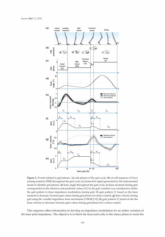
Sensors 2017, 17, 2751

0.5

Kn

ee

v

elo

city

(/s

)

-175

175

Ga

in

(u

.a.)

-0.5 Kn

ee

mo

me

nt

(Nm

/kg

)

1

FS

R

act

iva

tio

n

Swing

(S)

0

Ga

it

ph

ase

Initial

contact

(IC)

Mid

stance

(MS)

4

Kn

ee

an

gle

(

)

0

Ga

in

(u

.a.)

4

0

60

Gait cycle (%)

(a)

(b)

(c)

(d)

(e)

(f)

(g)

(h)

Inicial

contact

Loading

response

Mid

stance

Terminal

stance Swing

0

Terminal

Stance

(TS)

Moment reference

Moment predicted

Gain variation

0 16 54 60 100

VIKM gait velocity

Gain variation

4

Figure 2. Events related to gait phases. (a) sub-phases of the gait cycle; (b) on-off sequence of forcesensing resistors (FSR) throughout the gait cycle; (c) footswitch signal generated by the instrumentedinsole to identify gait phases; (d) knee angle throughout the gait cycle; (e) knee moment during gait,correspondent to the reference and predicted values of [21]; the gain variation was considered to definethe gait pattern to knee impedance modulation during gait; (f) gain pattern P1 based on the kneemoment to decrease/increase gain values during gait phases for stance control; (g) knee velocity duringgait using the variable impedance knee mechanism (VIKM) [38]; (h) gain pattern P2 based on the theknee velocity to decrease/increase gain values during gait phases for a stance control.

This sequence offers information to develop an impedance modulation for an online variation ofthe knee joint impedance. The objective is to block the knee joint only in the stance phase to resist the

178

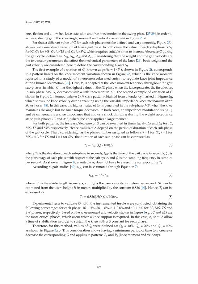
Sensors 2017, 17, 2751

knee flexion and allow free knee extension and free knee motion in the swing phase [25,39], in order toachieve, during gait, the knee angle, moment and velocity, as shown in Figure 2d–f.

For that, a different value of G for each sub-phase must be defined and vary smoothly. Figure 2f,hshows two examples of variation of G in a gait cycle. In both cases, the value for each sub-phase is G1

for IC, G2 for MS, G3 for TS and G4 for SW, which requires suitable times to increase/decrease G duringthe gait cycle, defined as: ∆t1, ∆t2, ∆t3 and ∆t4. Considering that the weight and the gait velocity arethe two major parameters that affect the mechanical parameters of the knee [26], both weight and thegait velocity are considered here to define the corresponding G and ∆t.

The first example of variation of G, known as pattern 1 (P1), shown in Figure 2f, correspondsto a pattern based on the knee moment variation shown in Figure 2e, which is the knee momentreported in a study of a model of a neuromuscular mechanism to regulate knee joint impedanceduring human locomotion [21]. Here, P1 is adapted at the knee moment tendency throughout the gaitsub-phases, in which G1 has the highest values in the IC phase when the knee generates the first flexion.In sub-phase MS, G2 decreases with a little increment in TS. The second example of variation of G

shown in Figure 2h, termed pattern 2 (P2), is a pattern obtained from a tendency marked in Figure 2g,which shows the knee velocity during walking using the variable impedance knee mechanism of anSC orthosis [38]. In this case, the highest value of G2 is generated in the sub-phase MS, when the kneemaintains the angle but the knee torque decreases. In both cases, an impedance modulation using P1

and P2 can generate a knee impedance that allows a shock damping during the weight acceptancestage (sub-phases IC and MS) where the knee applies a large moment.

For both patterns, the increase/decrease of G can be executed in times ∆1, ∆2, ∆3 and ∆4 for IC,MS, TS and SW, respectively. Hence, values of ∆ depend on the period of duration of each sub-phaseof the gait cycle. Then, considering i as the phase number assigned as follows: i = 1 for IC, i = 2 forMS, i = 3 for TS and i = 4 for SW, the duration of each sub-phase can be expressed as

Ti = tGC(Qi/100) fs, (6)

where Ti is the duration of each sub-phase in seconds, tGC is the time of the gait cycle in seconds, Qi isthe percentage of each phase with respect to the gait cycle, and fs is the sampling frequency in samplesper second. As shown in Figure 2f, a suitable ∆i does not have to exceed the corresponding Ti.

According to gait studies [40], tGC can be estimated through Equation 7:

tGC = SL/vu, (7)

where SL is the stride length in meters, and vu is the user velocity in meters per second. SL can beestimated from the users height H in meters multiplied by the constant 0.826 [40]. Hence, Ti can beexpressed as

Ti = 0.826(HQi fs)/100vu. (8)

Experimental tests to validate Qi with the instrumented insole were conducted, obtaining thefollowing percentages for each phase: 16 ± 4%, 38 ± 6%, 6 ± 0.8% and 40 ± 4% for IC, MS, TS andSW phases, respectively. Based on the knee moment and velocity shown in Figure 2e,g, IC and MS arethe more critical phases, which occur when a knee support is required. In this case, ∆t should allowa time of stabilization in order to sustain the knee with a G constant for each phase.

Therefore, for this method, values of Qi were defined as: Q1 = 10%; Q2 = 20% and Q4 = 40%,as shown in Figure 3a,b. This consideration allows having a minimum period of time to increase ordecrease the corresponding G and applies to patterns P1 and P2 (knee moment and velocity).

179

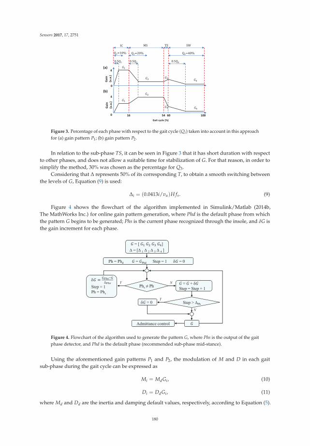
Sensors 2017, 17, 2751

Gait cycle (%)

(a)

(b)

0 16 54 60 100

G

ain

(u

.a.)

G

ain

(u

.a.)

0

4

4

Figure 3. Percentage of each phase with respect to the gait cycle (Qi) taken into account in this approachfor (a) gain pattern P1; (b) gain pattern P2.

In relation to the sub-phase TS, it can be seen in Figure 3 that it has short duration with respectto other phases, and does not allow a suitable time for stabilization of G. For that reason, in order tosimplify the method, 30% was chosen as the percentage for Q3.

Considering that ∆ represents 50% of its corresponding T, to obtain a smooth switching betweenthe levels of G, Equation (9) is used:

∆i = (0.0413i/vu)H fs. (9)

Figure 4 shows the flowchart of the algorithm implemented in Simulink/Matlab (2014b,The MathWorks Inc.) for online gain pattern generation, where Phd is the default phase from whichthe pattern G begins to be generated; Phs is the current phase recognized through the insole, and δG isthe gain increment for each phase.

Figure 4. Flowchart of the algorithm used to generate the pattern G, where Phs is the output of the gaitphase detector, and Phd is the default phase (recommended sub-phase mid-stance).

Using the aforementioned gain patterns P1 and P2, the modulation of M and D in each gaitsub-phase during the gait cycle can be expressed as

Mi = MdGi, (10)

Di = DdGi, (11)

where Md and Dd are the inertia and damping default values, respectively, according to Equation (5).

180

Sensors 2017, 17, 2751

2.3. Gait Phase Detection

The gait phase detection is required to implement the impedance modulation method proposedhere, which is done by the instrumented insole built with force sensing resistors (FSRs) shown inFigure 5a. Four FSRs are placed on the plantar surface of the foot. Figure 5b shows the sensorlocations, which are defined in the function of the peaks of the plantar pressure data reported in [41,42],corresponding to hallux bone (FSR1), 1st metatarsal (FSR2), 5th metatarsal (FSR3) and calcaneus (FSR4).These locations allow for acquiring more relevant ground reaction forces generated during gait torecognize stance sub-phases, which are suitable to use in feet with normal arch, high arch and flatfoot Figure 5c.

FSR1

FSR2

FSR3

FSR4

1

2

3

4

1

2

3

4

1

2

3

4

Flat arch High arch Normal

Figure 5. (a) instrumented insole implemented at the active knee orthosis; (b) FSR locations; (c) FSRlocations at flat arch, high arch and normal foot.

The sensors employed are FlexiForce A401 (Tekscan Inc, Boston, MA, USA), which areforce-sensing resistors with a sensing area of 25.4 mm and standard force range of 111 N. An electroniccircuit was implemented to obtain output voltages proportional to the plantar pressure. To validatethe insole data, a pressure sensitive gait mat GAITRite Electronic Walkway Platinum (CIR SystemsInc., Peekskill, NY, USA), 9 m long was employed. The signals of the insole were acquired with a DAQUSB-6009 (sampling frequency of 120 Hz) using the DAQ ExpressTM driver of National Instruments c©(Austin, TX, USA) and Matlab software. The mat data were acquired at 1 kHz using the PKMAS(ProtoKinetics Movement Analysis) software (Franklin, NJ, USA) [43]. The acquisition data weresynchronized throughout an external pulse. Two subjects (man: 35 years; 1.72 m; 70 kg and woman:78 years, 1.75 m, 80 kg) walked at a comfortable velocity on the mat using the insole. Each subjectcompleted six trials (each trial with six steps) completing 36 gait cycles. A concordance correlationanalysis was performed to estimate the reliability of the insole pressure signals in relation to the footpressure measured by the mat.Then, a gait phase detection algorithm based on a truth table from thecombinations of the sensors during gait was programed in Matlab Simulink. The signals were acquiredthrough an analog to digital acquisition card, model Diamond-MM-32DX-AT (32 inputs of 16 bits,4 outputs of 12 bits, with maximum sampling frequency of 250 kHz) of a PC-104 computer, sampled ata frequency of 1 kHz, and conditioned through a low-pass filter Butterworth of 5th-order, with cutofffrequency of 10 Hz. Afterwards, the signals were compared to a threshold of 0.5 V in order to obtaincontact information (on-off) from the footswitch. In order to recognize the gait sub-phases IC, MS, TS

and SW, the combinations shown in Figure 2b were considered. Then, a truth table implemented inSimulink/Matlab, which includes these combinations, was used to obtain a logic scheme to generatethe footswitch signal shown in Figure 2c.

181

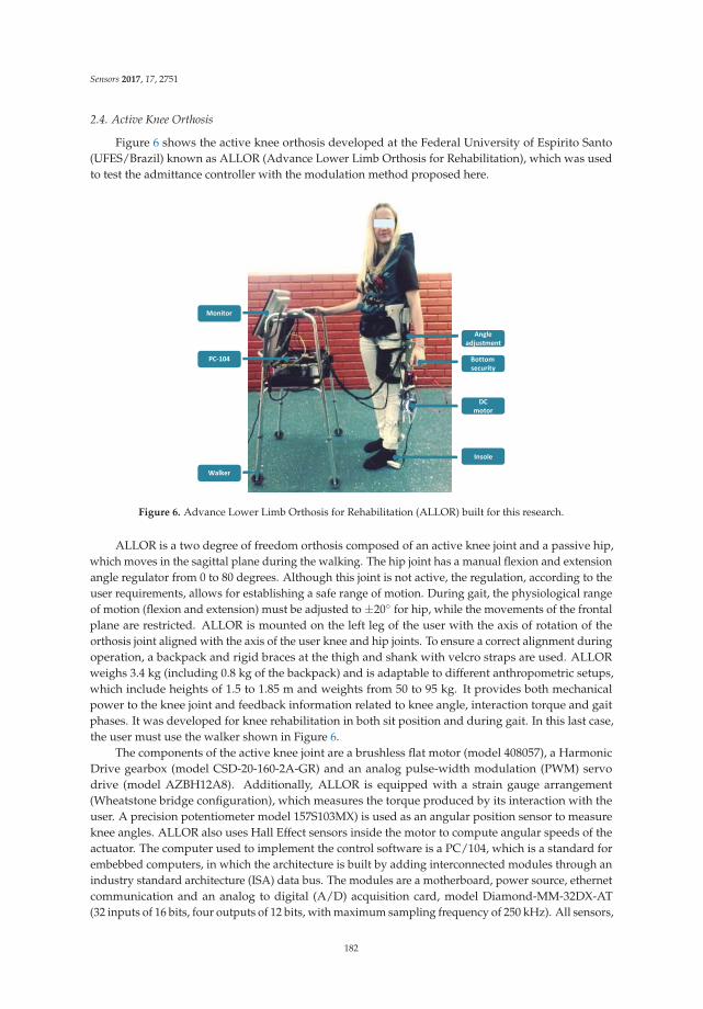
Sensors 2017, 17, 2751

2.4. Active Knee Orthosis

Figure 6 shows the active knee orthosis developed at the Federal University of Espirito Santo(UFES/Brazil) known as ALLOR (Advance Lower Limb Orthosis for Rehabilitation), which was usedto test the admittance controller with the modulation method proposed here.

DC

motor

Insole

Angle

adjustment

Bottom

security

Walker

PC-104

Monitor

Figure 6. Advance Lower Limb Orthosis for Rehabilitation (ALLOR) built for this research.

ALLOR is a two degree of freedom orthosis composed of an active knee joint and a passive hip,which moves in the sagittal plane during the walking. The hip joint has a manual flexion and extensionangle regulator from 0 to 80 degrees. Although this joint is not active, the regulation, according to theuser requirements, allows for establishing a safe range of motion. During gait, the physiological rangeof motion (flexion and extension) must be adjusted to ±20◦ for hip, while the movements of the frontalplane are restricted. ALLOR is mounted on the left leg of the user with the axis of rotation of theorthosis joint aligned with the axis of the user knee and hip joints. To ensure a correct alignment duringoperation, a backpack and rigid braces at the thigh and shank with velcro straps are used. ALLORweighs 3.4 kg (including 0.8 kg of the backpack) and is adaptable to different anthropometric setups,which include heights of 1.5 to 1.85 m and weights from 50 to 95 kg. It provides both mechanicalpower to the knee joint and feedback information related to knee angle, interaction torque and gaitphases. It was developed for knee rehabilitation in both sit position and during gait. In this last case,the user must use the walker shown in Figure 6.

The components of the active knee joint are a brushless flat motor (model 408057), a HarmonicDrive gearbox (model CSD-20-160-2A-GR) and an analog pulse-width modulation (PWM) servodrive (model AZBH12A8). Additionally, ALLOR is equipped with a strain gauge arrangement(Wheatstone bridge configuration), which measures the torque produced by its interaction with theuser. A precision potentiometer model 157S103MX) is used as an angular position sensor to measureknee angles. ALLOR also uses Hall Effect sensors inside the motor to compute angular speeds of theactuator. The computer used to implement the control software is a PC/104, which is a standard forembebbed computers, in which the architecture is built by adding interconnected modules through anindustry standard architecture (ISA) data bus. The modules are a motherboard, power source, ethernetcommunication and an analog to digital (A/D) acquisition card, model Diamond-MM-32DX-AT(32 inputs of 16 bits, four outputs of 12 bits, with maximum sampling frequency of 250 kHz). All sensors,

182

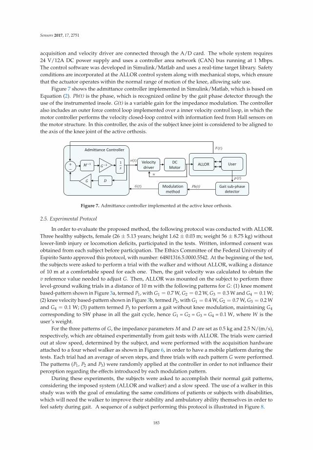
Sensors 2017, 17, 2751

acquisition and velocity driver are connected through the A/D card. The whole system requires24 V/12A DC power supply and uses a controller area network (CAN) bus running at 1 Mbps.The control software was developed in Simulink/Matlab and uses a real-time target library. Safetyconditions are incorporated at the ALLOR control system along with mechanical stops, which ensurethat the actuator operates within the normal range of motion of the knee, allowing safe use.

Figure 7 shows the admittance controller implemented in Simulink/Matlab, which is based onEquation (2). Ph(t) is the phase, which is recognized online by the gait phase detector through theuse of the instrumented insole. G(t) is a variable gain for the impedance modulation. The controlleralso includes an outer force control loop implemented over a inner velocity control loop, in which themotor controller performs the velocity closed-loop control with information feed from Hall sensors onthe motor structure. In this controller, the axis of the subject knee joint is considered to be aligned tothe axis of the knee joint of the active orthosis.

Velocity

driver

DC

Motor

ALLOR

Modulation

method

Admittance Controller

User

Gait sub-phase

detector

Figure 7. Admittance controller implemented at the active knee orthosis.

2.5. Experimental Protocol

In order to evaluate the proposed method, the following protocol was conducted with ALLOR.Three healthy subjects, female (26 ± 5.13 years; height 1.62 ± 0.03 m; weight 56 ± 8.75 kg) withoutlower-limb injury or locomotion deficits, participated in the tests. Written, informed consent wasobtained from each subject before participation. The Ethics Committee of the Federal University ofEspirito Santo approved this protocol, with number: 64801316.5.0000.5542. At the beginning of the test,the subjects were asked to perform a trial with the walker and without ALLOR, walking a distanceof 10 m at a comfortable speed for each one. Then, the gait velocity was calculated to obtain thev reference value needed to adjust G. Then, ALLOR was mounted on the subject to perform threelevel-ground walking trials in a distance of 10 m with the following patterns for G: (1) knee momentbased-pattern shown in Figure 3a, termed P1, with G1 = 0.7 W, G2 = 0.2 W, G3 = 0.3 W and G4 = 0.1 W;(2) knee velocity based-pattern shown in Figure 3b, termed P2, with G1 = 0.4 W, G2 = 0.7 W, G3 = 0.2 Wand G4 = 0.1 W; (3) pattern termed P3 to perform a gait without knee modulation, maintaining G4

corresponding to SW phase in all the gait cycle, hence G1 = G2 = G3 = G4 = 0.1 W, where W is theuser’s weight.

For the three patterns of G, the impedance parameters M and D are set as 0.5 kg and 2.5 N/(m/s),respectively, which are obtained experimentally from gait tests with ALLOR. The trials were carriedout at slow speed, determined by the subject, and were performed with the acquisition hardwareattached to a four wheel walker as shown in Figure 6, in order to have a mobile platform during thetests. Each trial had an average of seven steps, and three trials with each pattern G were performed.The patterns (P1, P2 and P3) were randomly applied at the controller in order to not influence theirperception regarding the effects introduced by each modulation pattern.

During these experiments, the subjects were asked to accomplish their normal gait patterns,considering the imposed system (ALLOR and walker) and a slow speed. The use of a walker in thisstudy was with the goal of emulating the same conditions of patients or subjects with disabilities,which will need the walker to improve their stability and ambulatory ability themselves in order tofeel safety during gait. A sequence of a subject performing this protocol is illustrated in Figure 8.

183

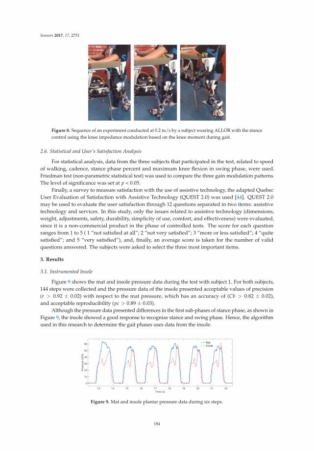
Sensors 2017, 17, 2751

Figure 8. Sequence of an experiment conducted at 0.2 m/s by a subject wearing ALLOR with the stancecontrol using the knee impedance modulation based on the knee moment during gait.

2.6. Statistical and User’s Satisfaction Analysis

For statistical analysis, data from the three subjects that participated in the test, related to speedof walking, cadence, stance phase percent and maximum knee flexion in swing phase, were used.Friedman test (non-parametric statistical test) was used to compare the three gain modulation patterns.The level of significance was set at p < 0.05.

Finally, a survey to measure satisfaction with the use of assistive technology, the adapted QuebecUser Evaluation of Satisfaction with Assistive Technology (QUEST 2.0) was used [44]. QUEST 2.0may be used to evaluate the user satisfaction through 12 questions separated in two items: assistivetechnology and services. In this study, only the issues related to assistive technology (dimensions,weight, adjustments, safety, durability, simplicity of use, comfort, and effectiveness) were evaluated,since it is a non-commercial product in the phase of controlled tests. The score for each questionranges from 1 to 5 ( 1 “not satisfied at all”; 2 “not very satisfied”; 3 “more or less satisfied”; 4 “quitesatisfied”; and 5 “very satisfied”), and, finally, an average score is taken for the number of validquestions answered. The subjects were asked to select the three most important items.

3. Results

3.1. Instrumented Insole

Figure 9 shows the mat and insole pressure data during the test with subject 1. For both subjects,144 steps were collected and the pressure data of the insole presented acceptable values of precision(r > 0.92 ± 0.02) with respect to the mat pressure, which has an accuracy of (Cb > 0.82 ± 0.02),and acceptable reproducibility (pc > 0.89 ± 0.03).

Although the pressure data presented differences in the first sub-phases of stance phase, as shown inFigure 9, the insole showed a good response to recognize stance and swing phase. Hence, the algorithmused in this research to determine the gait phases uses data from the insole.

Time (s)

13 14 15 16 17 18 19 20 21 22

Pre

ssu

re (

kP

a)

0

10

20

30

40

50

60Mat

Insole

Figure 9. Mat and insole plantar pressure data during six steps.

184

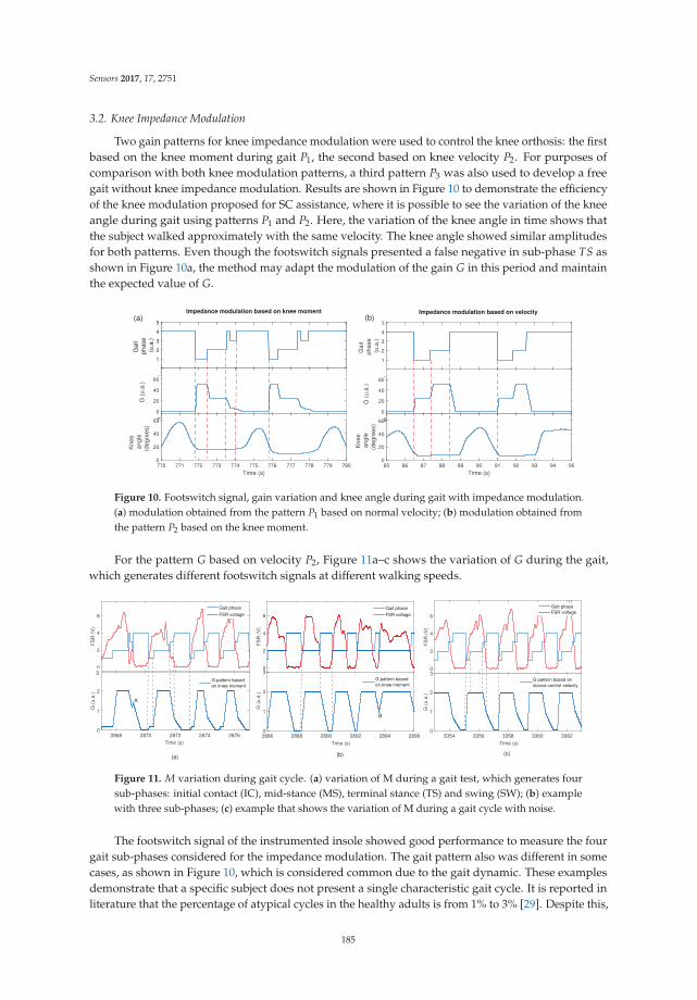
Sensors 2017, 17, 2751

3.2. Knee Impedance Modulation

Two gain patterns for knee impedance modulation were used to control the knee orthosis: the firstbased on the knee moment during gait P1, the second based on knee velocity P2. For purposes ofcomparison with both knee modulation patterns, a third pattern P3 was also used to develop a freegait without knee impedance modulation. Results are shown in Figure 10 to demonstrate the efficiencyof the knee modulation proposed for SC assistance, where it is possible to see the variation of the kneeangle during gait using patterns P1 and P2. Here, the variation of the knee angle in time shows thatthe subject walked approximately with the same velocity. The knee angle showed similar amplitudesfor both patterns. Even though the footswitch signals presented a false negative in sub-phase TS asshown in Figure 10a, the method may adapt the modulation of the gain G in this period and maintainthe expected value of G.

Time (s)

85 86 87 88 89 90 91 92 93 94 95

Ga

it

ph

ase

(u.a

.)0

1

2

3

4

5

Impedance modulation based on velocity

Time (s)

85 86 87 88 89 90 91 92 93 94 95

G (

u.a

.)

0

20

40

60

80

Time (s)

85 86 87 88 89 90 91 92 93 94 95

Kn

ee

an

gle

(de

gre

es)

0

20

40

60

Time (s)

770 771 772 773 774 775 776 777 778 779 780

Ga

it

ph

ase

(u.a

.)

0

1

2

3

4

5

Impedance modulation based on knee moment

770 771 772 773 774 775 776 777 778 779 780

G (

u.a

.)

0

20

40

60

80

Time (s)

770 771 772 773 774 775 776 777 778 779 780

Kn

ee

an

gle

(de

gre

es)

0

20

40

60

(a) (b)

Figure 10. Footswitch signal, gain variation and knee angle during gait with impedance modulation.(a) modulation obtained from the pattern P1 based on normal velocity; (b) modulation obtained fromthe pattern P2 based on the knee moment.

For the pattern G based on velocity P2, Figure 11a–c shows the variation of G during the gait,which generates different footswitch signals at different walking speeds.

Time (s)

2868 2870 2872 2874 2876

FS

R (

V)

0

2

4

6

Gait phase

FSR voltage

Time (s)

2868 2870 2872 2874 2876

G (

u.a

.)

0

1

2

3

G pattern based

on knee moment Time (s)

3354 3356 3358 3360 3362

FS

R (

V)

0

2

4

6

Gait phase

FSR voltage

Time (s)

3354 3356 3358 3360 3362

G (

u.a

.)

0

1

2

3G pattern based on

stance control velocityTime (s)

2886 2888 2890 2892 2894 2896

FS

R (

V)

0

2

4

6

Gait phase

FSR voltage

Time (s)

2886 2888 2890 2892 2894 2896

G (

u.a

.)

0

1

2

3

G pattern based

on knee moment

A

B

3.

(a) (b) (c)

Figure 11. M variation during gait cycle. (a) variation of M during a gait test, which generates foursub-phases: initial contact (IC), mid-stance (MS), terminal stance (TS) and swing (SW); (b) examplewith three sub-phases; (c) example that shows the variation of M during a gait cycle with noise.

The footswitch signal of the instrumented insole showed good performance to measure the fourgait sub-phases considered for the impedance modulation. The gait pattern also was different in somecases, as shown in Figure 10, which is considered common due to the gait dynamic. These examplesdemonstrate that a specific subject does not present a single characteristic gait cycle. It is reported inliterature that the percentage of atypical cycles in the healthy adults is from 1% to 3% [29]. Despite this,

185

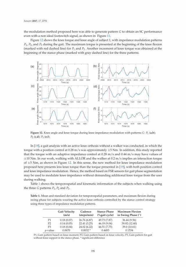
Sensors 2017, 17, 2751

the modulation method proposed here was able to generate pattern G to obtain an SC performanceeven with a non ideal footswitch signal, as shown in Figure 11.

Figure 12 shows the knee torque and knee angle of subject 1, with impedance modulation patternsP1, P2, and P3 during the gait. The maximum torque is presented at the beginning of the knee flexion(marked with red dashed line) for P1 and P2. Another increment of knee torque was obtained at thebeginning of the stance phase (marked with gray dashed line) for the three patterns.

Time (s)

2908 2910 2912 2914 2916 2918 2920 2922Knee a

ngle

(degre

es)

0

20

40

60

Time (s)

1416 1418 1420 1422 1424 1426 1428Knee a

ngle

(degre

es)

0

20

40

60

Time (s)

1670 1672 1674 1676 1678 1680 1682Knee a

ngle

(degre

es)

0

20

40

Time (s)

2908 2910 2912 2914 2916 2918 2920 2922

Knee torq

ue (

Nm

)

-5

0

5

Time (s)

1416 1418 1420 1422 1424 1426 1428

Knee torq

ue (

Nm

)-5

0

5

Time (s)

1670 1672 1674 1676 1678 1680 1682

Knee torq

ue (

Nm

)

-5

0

5

(a) (b)

(c) (d)

(e) (f)

Figure 12. Knee angle and knee torque during knee impedance modulation with patterns G: P1 (a,b);P2 (c,d); P3 (e,f).

In [19], a gait analysis with an active knee orthosis without a walker was conducted, in which thetorque with a position control at 0.28 m/s was approximately ±5 Nm. In addition, this study reportedthat the torque with an adaptive impedance control at 0.28 m/s and 0.44 m/s may have values of±10 Nm. In our work, walking with ALLOR and the walker at 0.2 m/s implies an interaction torqueof ±5 Nm, as shown in Figure 12. In this sense, the new method for knee impedance modulationproposed here presents less knee torque than the torque presented in [19], with both position controland knee impedance modulation. Hence, the method based on FSR sensors for gait phase segmentationmay be used to modulate knee impedance without demanding additional knee torque from the userduring walking.

Table 1 shows the temporospatial and kinematic information of the subjects when walking usingthe three G patterns P1, P2 and P3.

Table 1. Mean and standard deviation for temporospatial parameters, and maximum flexion duringswing phase for subjects wearing the active knee orthosis controlled by the stance control strategyusing three types of impedance modulation patterns.

Gait Velocity Cadence Stance Phase Maximum Flexion(m/s) (steps/min) (%gait cycle) in Swing Phase (◦)

P1 0.18 (0.07) 26.76 (6.87) 49.73 (7.87) 36.44 (9.56)P2 0.14 (0.05) 22.41 (3.25) 46.19 (9.04) 39.92 (12.40)P3 0.18 (0.04) 24.02 (6.22) 44.51 (7.75) 39.0 (10.61)

p-value 0.0670 0.0032 * 0.4493 0.1534

P1, Gain pattern based on knee moment; P2, Gain pattern based on knee velocity; P3, Gain pattern for gaitwithout knee support in the stance phase. * significant difference

186

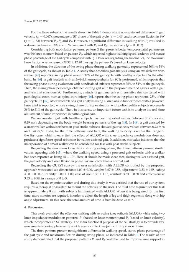
Sensors 2017, 17, 2751

For the three subjects, the results shown in Table 1 demonstrate no significant difference in gaitvelocity (p = 0.067), percentage of ST phase of the gait cycle (p = 0.44) and maximum flexion in SW(p = 0.153) between P1, P2 and P3. However, a significant difference in walking with P2 resulted ina slower cadence in 16% and 10% compared with P1 and P3, respectively (p = 0.0032).

Considering both modulation patterns, pattern G that presents better temporospatial parameterswas the knee moment based on pattern P1, which reported highest walking speed, cadence and stancephase percentage of the gait cycle compared with P2. However, regarding the kinematics, the maximumknee flexion was increased (39.92 ± 12.40◦) using the pattern P2 based on knee velocity.

In addition, the duration of the swing phase during walking generally represented 50% to 56%of the gait cycle, as shown in Table 1. A study that describes gait analysis using an exoskeleton withwalker [45] reports a swing phase around 37% of the gait cycle with healthy subjects. On the otherhand, in [46] , a gait analysis with an hybrid neuroprosthesis for SC is performed, which reports thatthe swing phase during evaluation with nondisabled subjects represents 36% to 51% of the gait cycle.Then, the swing phase percentage obtained during gait with the proposed method agrees with a gaitanalysis that considers SC. Furthermore, a study of gait analysis with assistive devices tested withpathological cases, such as spinal cord injury [46], reports that the swing phase represents 25% of thegait cycle. In [47], other research of a gait analysis using a knee-ankle-foot orthoses with a poweredknee joint is reported, whose swing phase during evaluation with poliomyelitis subjects represents36% to 51% of the gait cycle. Then, in this sense, an important future task is to analyze the real-timeadjustment of knee impedance in pathological gait.

Walker assisted gait with healthy subjects has been reported values between 0.17 m/s and0.29 m/s depending on the body weight bearing patterns of the leg [48]. In [49], a gait assisted bya smart walker without orthosis in post-stroke subjects showed gait velocity values between 0.23 m/sand 0.44 m/s. Then, for the three patterns used here, the walking velocity is within that range ofthe first case, which means that the effect of ALLOR with knee impedance modulation does notproduce a significant speed reduction in walker-assisted gait. In addition, this value indicates that theincorporation of a smart walker can be considered for test with post-stroke subjects.

Regarding the maximum knee flexion during swing phase, the three patterns present similarvalues, agreeing with [45], where the walking speed using a powered gait orthosis with a walkerhas been reported as being 48 ± 10◦. Here, it should be made clear that, during walker assisted gait,the gait velocity and knee flexion in phase SW are lower than a normal gait.

Regarding the QUEST survey, the user satisfaction with ALLOR controlled by the proposedapproach was scored as: dimensions: 4.00 ± 0.00, weight: 3.67 ± 0.58, adjustment: 3.33 ± 0.58, safety:4.00 ± 0.00, durability: 3.00 ± 1.00, ease of use: 3.33 ± 1.15, comfort: 3.33 ± 0.58 and effectiveness:3.33 ± 0.58, in a range of 0 to 5.

Based on the experience after and during this study, it was verified that the use of our systemrequires a therapist or assistant to mount the orthosis on the user. The total time required for this taskis approximately 8 min with subjects familiarized with ALLOR. When it is being used for the firsttime, more minutes are required, in order to adjust the length of leg and thigh segments along with hipangle adjustment. In this case, the total amount of time is from be 20 to 25 min.

4. Discussion

This work evaluated the effect on walking with an active knee orthosis (ALLOR) while using twoknee impedance modulation patterns: P1 (based on knee moment) and P2 (based on knee velocity),which incorporates an SC strategy. The main functional purpose of the SC strategy is to provide freemovements in swing phase and provide a support to knee joints during stance phase.

The three patterns present no significant difference in walking speed, stance phase percentage ofthe gait cycle and maximum flexion during swing phase, as indicated in Table 1. The results of ourstudy demonstrated that the proposed patterns P1 and P2 could be used to improve knee support in

187

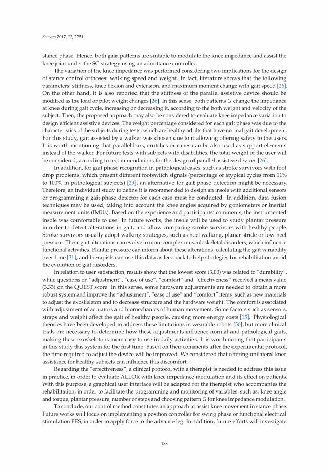
Sensors 2017, 17, 2751

stance phase. Hence, both gain patterns are suitable to modulate the knee impedance and assist theknee joint under the SC strategy using an admittance controller.

The variation of the knee impedance was performed considering two implications for the designof stance control orthoses: walking speed and weight. In fact, literature shows that the followingparameters: stiffness, knee flexion and extension, and maximum moment change with gait speed [26].On the other hand, it is also reported that the stiffness of the parallel assistive device should bemodified as the load or pilot weight changes [26]. In this sense, both patterns G change the impedanceat knee during gait cycle, increasing or decreasing it, according to the both weight and velocity of thesubject. Then, the proposed approach may also be considered to evaluate knee impedance variation todesign efficient assistive devices. The weight percentage considered for each gait phase was due to thecharacteristics of the subjects during tests, which are healthy adults that have normal gait development.For this study, gait assisted by a walker was chosen due to it allowing offering safety to the users.It is worth mentioning that parallel bars, crutches or canes can be also used as support elementsinstead of the walker. For future tests with subjects with disabilities, the total weight of the user willbe considered, according to recommendations for the design of parallel assistive devices [26].

In addition, for gait phase recognition in pathological cases, such as stroke survivors with footdrop problems, which present different footswitch signals (percentage of atypical cycles from 11%to 100% in pathological subjects) [29], an alternative for gait phase detection might be necessary.Therefore, an individual study to define it is recommended to design an insole with additional sensorsor programming a gait-phase detector for each case must be conducted. In addition, data fusiontechniques may be used, taking into account the knee angles acquired by goniometers or inertialmeasurement units (IMUs). Based on the experience and participants’ comments, the instrumentedinsole was comfortable to use. In future works, the insole will be used to study plantar pressurein order to detect alterations in gait, and allow comparing stroke survivors with healthy people.Stroke survivors usually adopt walking strategies, such as heel walking, planar stride or low heelpressure. These gait alterations can evolve to more complex musculoskeletal disorders, which influencefunctional activities. Plantar pressure can inform about these alterations, calculating the gait variabilityover time [31], and therapists can use this data as feedback to help strategies for rehabilitation avoidthe evolution of gait disorders.

In relation to user satisfaction, results show that the lowest score (3.00) was related to “durability”,while questions on “adjustment”, “ease of use”, “comfort” and “effectiveness” received a mean value(3.33) on the QUEST score. In this sense, some hardware adjustments are needed to obtain a morerobust system and improve the “adjustment”, “ease of use” and “comfort” items, such as new materialsto adjust the exoskeleton and to decrease structure and the hardware weight. The comfort is associatedwith adjustment of actuators and biomechanics of human movement. Some factors such as sensors,straps and weight affect the gait of healthy people, causing more energy costs [15]. Physiologicaltheories have been developed to address these limitations in wearable robots [50], but more clinicaltrials are necessary to determine how these adjustments influence normal and pathological gaits,making these exoskeletons more easy to use in daily activities. It is worth noting that participantsin this study this system for the first time. Based on their comments after the experimental protocol,the time required to adjust the device will be improved. We considered that offering unilateral kneeassistance for healthy subjects can influence this discomfort.

Regarding the “effectiveness”, a clinical protocol with a therapist is needed to address this issuein practice, in order to evaluate ALLOR with knee impedance modulation and its effect on patients.With this purpose, a graphical user interface will be adapted for the therapist who accompanies therehabilitation, in order to facilitate the programming and monitoring of variables, such as: knee angleand torque, plantar pressure, number of steps and choosing pattern G for knee impedance modulation.

To conclude, our control method constitutes an approach to assist knee movement in stance phase.Future works will focus on implementing a position controller for swing phase or functional electricalstimulation FES, in order to apply force to the advance leg. In addition, future efforts will investigate

188

Sensors 2017, 17, 2751

correlations between the FSR activation and the knee joint impedance during walking on treadmillsand stair climbing.

Acknowledgments: This work was supported by CNPq (304192/2016-3), CAPES (88887.095626/2015-01), FAPES(72982608) (Brazil), and SENESCYT (Convocatoria Abierta 2012) (Ecuador). We thank the members of the ALLORteam for supporting the research.

Author Contributions: A.C.V.-P. developed the knee exoskeleton and controller, performed the experiments,analyzed the data and drafted the manuscript. D.D.-R. contributed to designing the experimental protocol, draftingthe manuscript and analyzed the data. J.S.L. designed the experimental protocol, contributed to performing theexperiments, and analyzed the data and interpretation of findings. A.F.-N. and T.B. contributed with materialsand analysis tools, and contributed to the data analysis and interpretation of the findings. All authors read, edited,and approved the final manuscript.

Conflicts of Interest: The authors declare no conflict of interest.

Abbreviations

The following abbreviations are used in this manuscript:

ALLOR Advance Lower Limb Orthosis for RehabilitationD DampingF ForceFSR Force sensing resistorG Gain for impedance modulationH ALLOR user’s heightIC Initial contact phaseM Massp Plantar pressureP1 Gain pattern for impedance modulation based on knee moment during gaitP2 Gain pattern for impedance modulation based on knee velocity during gaitP3 Gain pattern for impedance modulation to obtain a free movementPh PhaseQ PercentageQUEST Quebec User Evaluation of Satisfaction with Assistive TechnologySC Stance controlST Stance phaseSW Swing phaset TimeW ALLOR user’s weight

References

1. Mahlknecht, P.; Kiechl, S.; Bloem, B.R.; Willeit, J.; Scherfler, C.; Gasperi, A.; Rungger, G.; Poewe, W.; Seppi, K.Prevalence and Burden of Gait Disorders in Elderly Men and Women Aged 60–97 Years: A Population-BasedStudy. PLoS ONE 2013, 8, e69627.

2. Balaban, B.; Tok, F. Gait Disturbances in Patients With Stroke. PM&R 2014, 6, 635–642.3. Salzman, B. Gait and balance disorders in older adults. Am. Fam. Physician 2010, 82, 61–68.4. Hendrickson, J.; Patterson, K.K.; Inness, E.L.; McIlroy, W.E.; Mansfield, A. Relationship between asymmetry

of quiet standing balance control and walking post-stroke. Gait Posture 2014, 39, 177–181.5. Weerdesteyn, V.; de Niet, M.; van Duijnhoven, H.J.R.; Geurts, A.C.H. Falls in individuals with stroke. J. Rehabil.

Res. Dev. 2008, 45, 1195–1213.6. Dzahir, M.A.M.; Yamamoto, S.I. Recent trends in lower-limb robotic rehabilitation orthosis: Control scheme

and strategy for pneumatic muscle actuated gait trainers. Robotics 2014, 3, 120–148.7. Tucker, M.R.; Olivier, J.; Pagel, A.; Bleuler, H.; Bouri, M.; Lambercy, O.; del R Millán, J.; Riener, R.;

Vallery, H.; Gassert, R. Control strategies for active lower extremity prosthetics and orthotics: A review.J. Neuroeng. Rehabilit. 2015, 12, 1.

189

Sensors 2017, 17, 2751

8. Chen, B.; Ma, H.; Qin, L.Y.; Gao, F.; Chan, K.M.; Law, S.W.; Qin, L.; Liao, W.H. Recent developments andchallenges of lower extremity exoskeletons. J. Orthop. Transl. 2016, 5, 26–37.

9. Villa-Parra, A.; Broche, L.; Delisle-Rodríguez, D.; Sagaró, R.; Bastos, T.; Frizera-Neto, A. Design of activeorthoses for a robotic gait rehabilitation system. Front. Mech. Eng. 2015, 10, 242–254.

10. Louie, D.R.; Eng, J.J. Powered robotic exoskeletons in post-stroke rehabilitation of gait: A scoping review.J. Neuroeng. Rehabilit. 2016, 13, 53.

11. Louie, D.R.; Eng, J.J.; Lam, T. Gait speed using powered robotic exoskeletons after spinal cord injury:A systematic review and correlational study. J. Neuroeng. Rehabilit. 2015, 12, 82.

12. Cao, J.; Xie, S.Q.; Das, R.; Zhu, G.L. Control strategies for effective robot assisted gait rehabilitation: The stateof art and future prospects. Med. Eng. Phys. 2014, 36, 1555–1566.

13. Tsuji, T.; Tanaka, Y. Tracking control properties of human-robotic systems based on impedance control.IEEE Trans. Syst. Man Cybern. Part A Syst. Hum. 2005, 35, 523–535.

14. Hussain, S.; Xie, S.Q.; Jamwal, P.K. Adaptive impedance control of a robotic orthosis for gait rehabilitation.IEEE Trans. Cybern. 2013, 43, 1025–1034.

15. Huo, W.; Mohammed, S.; Moreno, J.C.; Amirat, Y. Lower limb wearable robots for assistance and rehabilitation:A state of the art. IEEE Syst. J. 2016, 10, 1068–1081.

16. Bulea, T.C.; Kobetic, R.; To, C.S.; Audu, M.L.; Schnellenberger, J.R.; Triolo, R.J. A variable impedance kneemechanism for controlled stance flexion during pathological gait. IEEE/ASME Trans. Mechatron. 2012,17, 822–832.

17. Ajoudani, A. Transferring Human Impedance Regulation Skills to Robots; Springer: Berlin, Heidelberg, 2016.18. Meng, W.; Liu, Q.; Zhou, Z.; Ai, Q.; Sheng, B.; Xie, S.S. Recent development of mechanisms and control

strategies for robot-assisted lower limb rehabilitation. Mechatronics 2015, 31, 132–145.19. Figueiredo, J.; Félix, P.; Santos, C.P.; Moreno, J.C. Towards human-knee orthosis interaction based on

adaptive impedance control through stiffness adjustment. IEEE Int. Conf. Rehabil. Robot. 2017, 406–411.doi:10.1109/ICORR.2017.8009281.

20. Pfeifer, S.; Vallery, H.; Hardegger, M.; Riener, R.; Perreault, E.J. Model-based estimation of knee stiffness.IEEE Trans. Biomed. Eng. 2012, 59, 2604–2612.

21. Sartori, M.; Maculan, M.; Pizzolato, C.; Reggiani, M.; Farina, D. Modeling and simulating the neuromuscularmechanisms regulating ankle and knee joint stiffness during human locomotion. J. Neurophysiol. 2015,114, 2509–2527.

22. Rafiaei, M.; Bahramizadeh, M.; Arazpour, M.; Samadian, M.; Hutchins, S.; Farahmand, F.; Mardani, M. The gaitand energy efficiency of stance control knee-ankle-foot orthoses: A literature review. Prosthet. Orthot. Int. 2016,40, 202–214.

23. Zissimopoulos, A.; Fatone, S.; Gard, S.A. Biomechanical and energetic effects of a stance-control orthoticknee joint. J. Rehabilitat. Res. Dev. 2007, 44, 503–513.

24. Zacharias, B.; Kannenberg, A. Clinical Benefits of Stance Control Orthosis Systems: An Analysis of theScientific Literature. J. Prosthet. Orthot. 2012, 24, 2–7.

25. Ir, M.; Azuan, N. Stance-Control-Orthoses with Electromechanical Actuation Mechanism: Usefulness, DesignAnalysis and Directions to Overcome Challenges. J. Neurol. Neurosci. 2015, doi:10.21767/2171-6625.100049.

26. Shamaei, K.; Dollar, A.M. On the mechanics of the knee during the stance phase of the gait. IEEE Int. Conf.

Rehabil. Robot. 2011, 2011, 5975478, doi:10.1109/ICORR.2011.5975478.27. Yakimovich, T.; Lemaire, E.D.; Kofman, J. Engineering design review of stance-control knee-ankle-foot

orthoses. J. Rehabilit. Res. Dev. 2009, 46, 257.28. Han, Y.; Cao, Y.; Zhao, J.; Yin, Y.; Ye, L.; Wang, X.; You, Z. A self-powered insole for human motion recognition.

Sensors 2016, 16, 1502.29. Agostini, V.; Balestra, G.; Knaflitz, M. Segmentation and classification of gait cycles. IEEE Trans. Neural Syst.

Rehabilit. Eng. 2014, 22, 946–952.30. Shahabpoor, E.; Pavic, A. Measurement of walking ground reactions in real-life environments: A systematic

review of techniques and technologies. Sensors 2017, 17, 2085.31. Munoz-Organero, M.; Parker, J.; Powell, L.; Mawson, S. Assessing walking strategies using insole pressure

sensors for stroke survivors. Sensors 2016, 16, 1631.32. Moufawad El Achkar, C.; Lenoble-Hoskovec, C.; Paraschiv-Ionescu, A.; Major, K.; Büla, C.; Aminian, K.

Physical behavior in older persons during daily life: Insights from instrumented shoes. Sensors 2016, 16, 1225.

190

Sensors 2017, 17, 2751

33. Tucker, M.R.; Moser, A.; Lambercy, O.; Sulzer, J.; Gassert, R. Design of a wearable perturbator forhuman knee impedance estimation during gait. IEEE Int. Conf. Rehabil. Robot. 2013, 2013, 6650372,doi:10.1109/ICORR.2013.6650372.

34. Espinosa, D.A. Hybrid Walking Therapy with Fatigue Management for Spinal Cord Injured Individuals.Ph.D. Thesis, Carlos III University, Madrid, Spain, 2013.

35. Buerger, S.P.; Hogan, N. Impedance and Interaction Control. In Robotics and Automation Handbook; CRC Press:Boca Raton, FL, USA, 2005.

36. Newman, W.S. Stability and Performance Limits of Interaction Controllers. J. Dyn. Syst. Meas. Control 1992,114, 563–570.

37. Chen, B.; Zheng, E.; Wang, Q.; Wang, L. A new strategy for parameter optimization to improve phase-dependentlocomotion mode recognition. Neurocomputing 2015, 149, 585–593.

38. Bulea, T.C.; Kobetic, R.; Triolo, R.J. Restoration of stance phase knee flexion during walking after spinal cordinjury using a variable impedance orthosis. Conf. Proc. IEEE Eng. Med. Biol. Soc. 2011, 2011, 608–611.

39. Yan, T.; Cempini, M.; Oddo, C.M.; Vitiello, N. Review of assistive strategies in powered lower-limb orthosesand exoskeletons. Robot. Auton. Syst. 2015, 64, 120–136.

40. Arnos, P. Age-Related Changes in Gait: Influence of Upper-Body Posture. Ph.D. Thesis, University of Toledo,Madrid, Spain, 2007.

41. Wafai, L.; Zayegh, A.; Woulfe, J.; Aziz, S.M.; Begg, R. Identification of Foot Pathologies Based on PlantarPressure Asymmetry. Sensors 2015, 15, 20392–20408.

42. Callaghan, M.; Whitehouse, S.; Baltzopoulos, V.; Samarji, R. A Comparison of the Effects of FirstMetatarsophalangeal Joint Arthrodesis and Hemiarthroplasty on Function of Foot Forces using Gait Analysis.Foot Ankle Online J. 2011, 4, 1.

43. Lynall, R.C.; Zukowski, L.A.; Plummer, P.; Mihalik, J.P. Reliability and validity of the protokinetics movementanalysis software in measuring center of pressure during walking. Gait Posture 2017, 52, 308–311.

44. De Carvalho, K.E.C.; Júnior, G.; Bolívar, M.; Sá, K.N. Translation and validation of the Quebec UserEvaluation of Satisfaction with Assistive Technology (QUEST 2.0) into Portuguese. Rev. Bras. Reumatol. 2014,54, 260–267.

45. Kang, S.J.; Ryu, J.C.; Moon, I.H.; Kim, K.H.; Mun, M.S. Walker gait analysis of powered gait orthosis forparaplegic. In World Congress on Medical Physics and Biomedical Engineering 2006; Springer: Berlin, Heidelberg,2007; pp. 2889–2891.

46. To, C.S.; Kobetic, R.; Bulea, T.C.; Audu, M.L.; Schnellenberger, J.R.; Pinault, G.; Triolo, R.J. Stance controlknee mechanism for lower-limb support in hybrid neuroprosthesis. J. Rehabil. Res. Dev. 2011, 48, 839.

47. Arazpour, M.; Moradi, A.; Samadian, M.; Bahramizadeh, M.; Joghtaei, M.; Ahmadi Bani, M.; Hutchins, S.W.;Mardani, M.A. The influence of a powered knee–ankle–foot orthosis on walking in poliomyelitis subjects:A pilot study. Prosthet. Orthot. Int. 2016, 40, 377–383.

48. Bachschmidt, R.A.; Harris, G.F.; Simoneau, G.G. Walker-assisted gait in rehabilitation: A study of biomechanicsand instrumentation. IEEE Trans. Neural Syst. Rehabilit. Eng. 2001, 9, 96–105.

49. Loterio, F.A.; Valadão, C.T.; Cardoso, V.F.; Pomer-Escher, A.; Bastos, T.F.; Frizera-Neto, A. Adaptation ofa smart walker for stroke individuals: A study on sEMG and accelerometer signals. Res. Biomed. Eng. 2017,doi:10.1590/2446-4740.01717.

50. Li, J.; Zhang, Z.; Tao, C.; Ji, R. Structure design of lower limb exoskeletons for gait training. Chin. J. Mech. Eng.

2015, 28, 878–887.

c© 2017 by the authors. Licensee MDPI, Basel, Switzerland. This article is an open accessarticle distributed under the terms and conditions of the Creative Commons Attribution(CC BY) license (http://creativecommons.org/licenses/by/4.0/).

191

MDPI

St. Alban-Anlage 66

4052 Basel

Switzerland

Tel. +41 61 683 77 34

Fax +41 61 302 89 18

www.mdpi.com

Sensors Editorial Office

E-mail: sensors@mdpi.com

www.mdpi.com/journal/sensors

MDPI

St. Alban-Anlage 66

4052 Basel

Switzerland

Tel: +41 61 683 77 34

Fax: +41 61 302 89 18

www.mdpi.com ISBN 978-3-03897-395-9