Input-output biomolecular systems Rushina Shah

Input-output biomolecular systems

by

Rushina Shah

Submitted to the Department of Mechanical Engineeringin partial fulfillment of the requirements for the degree of

Doctor of Philosophy in Mechanical Engineering

at the

MASSACHUSETTS INSTITUTE OF TECHNOLOGY

September 2020

c Massachusetts Institute of Technology 2020. All rights reserved.

Author . . . . . . . . . . . . . . . . . . . . . . . . . . . . . . . . . . . . . . . . . . . . . . . . . . . . . . . . . . . . . . . .Department of Mechanical Engineering

July 24, 2020

Certified by. . . . . . . . . . . . . . . . . . . . . . . . . . . . . . . . . . . . . . . . . . . . . . . . . . . . . . . . . . . .Domitilla Del Vecchio

ProfessorThesis Supervisor

Accepted by . . . . . . . . . . . . . . . . . . . . . . . . . . . . . . . . . . . . . . . . . . . . . . . . . . . . . . . . . . .Professor Nicolas G. Hadjiconstantinou

Graduate Officer

2

Input-output biomolecular systems

by

Rushina Shah

Submitted to the Department of Mechanical Engineeringon July 24, 2020, in partial fulfillment of the

requirements for the degree ofDoctor of Philosophy in Mechanical Engineering

Abstract

The ability of cells to sense and respond to their environment is encoded in biomolecu-lar reaction networks, in which information travels through processes such as production,modification, and removal of biomolecules. These reaction networks can be modeled asinput-output systems, where the input, state and output variables are concentrations of thebiomolecules involved in these reactions. Tools from non-linear dynamics and control theorycan be leveraged to analyze and control these systems. In this thesis, we study two keybiomolecular networks.

In part 1 of this thesis, we study the input-output behavior of signaling systems, which areresponsible for the transmission of information both from outside and from within the cells,and are ubiquitous, playing a role in cell cycle progression, survival, growth, differentiationand apoptosis. A signaling pathway transmits information from an upstream system todownstream systems, ideally in a unidirectional fashion. A key obstacle to unidirectionaltransmission is retroactivity, the additional reaction flux that affects a system once its speciesinteract with those of downstream systems. In this work, we identify signaling architecturesthat can overcome retroactivity, allowing unidirectional transmission of signals. These find-ings can be used to decompose natural signal transduction networks into modules, and atthe same time, they establish a library of devices that can be used in synthetic biology tofacilitate modular circuit design.

In part 2 of this thesis, we design inputs to trigger a transition of cell-fate from one celltype to another. The process of cell-fate decision-making is often modeled by means ofmultistable gene regulatory networks, where different stable steady states represent distinctcell phenotypes. In this thesis, we provide theoretical results that guide the selection ofinputs that trigger a transition, i.e., reprogram the network, to a desired stable steady state.Our results depend uniquely on the structure of the network and are independent of specificparameter values. We demonstrate these results by means of several examples, includingmodels of the extended network controlling stem-cell maintenance and differentiation.

Thesis Supervisor: Domitilla Del VecchioTitle: Professor

3

4

Acknowledgments

I would like to express my sincere gratitude to my advisor, Professor Domitilla Del

Vecchio, for her guidance during my graduate studies. Her immense knowledge and

commitment to rigor have been illuminating and inspiring. This thesis would not

have been possible without her continuing patience and motivation.

I would also like to thank the members of my thesis committee, Professor Harry

Asada and Professor Jean-Jacques Slotine, for their invaluable feedback and constant

encouragement.

I am very grateful for the support and friendship of the past and present members

of the Del Vecchio group. I would especially like to thank Yili Qian and Theodore

Grunberg for answering my many questions, and stimulating discussions; Narmada

Herath, Heejin Ahn, Cameron McBride and Penny Chen for their friendship; and

the entire group for creating an extremely friendly and inspiring work environment.

I would also like to thank Joe Gaken for his assistance with every administrative need.

I am deeply grateful to all my friends at MIT for their support and company through

this journey. Further, this journey would not have been possible without my friends

from my undergraduate studies at IIT Bombay, or without the support and encour-

agement from my Bachelors’ thesis advisor, Professor Abhishek Gupta.

Lastly, I would like to thank my parents and my younger brother for their love,

support, and encouragement.

5

6

Contents

1 Introduction 29

1.1 Motivation . . . . . . . . . . . . . . . . . . . . . . . . . . . . . . . . . 29

1.2 Statement of Contributions . . . . . . . . . . . . . . . . . . . . . . . 35

I Signaling Systems 38

2 Problem Statement 39

2.1 Example . . . . . . . . . . . . . . . . . . . . . . . . . . . . . . . . . . 41

3 Generalized Model 45

3.1 Simulations and Validity of Results . . . . . . . . . . . . . . . . . . . 48

4 Results: A Procedure to Evaluate Signaling Motifs and a Library of

Insulation Devices 49

4.1 Procedure to Determine Unidirectional Signal Transmission . . . . . . 50

4.2 Double phosphorylation cycle with input as kinase . . . . . . . . . . . 53

4.3 Regulated autophosphorylation followed by phosphotransfer . . . . . 55

4.4 Cascade of single phosphorylation cycles . . . . . . . . . . . . . . . . 58

4.5 Phosphotransfer with the phosphate donor undergoing autophospho-

rylation as input . . . . . . . . . . . . . . . . . . . . . . . . . . . . . 61

4.6 Single cycle with substrate input . . . . . . . . . . . . . . . . . . . . 64

5 Conclusions 68

7

II Reprogramming multistable gene regulatory networks 71

6 Motivating examples 72

7 Background and Problem Statement 76

7.1 Background: Monotone Systems . . . . . . . . . . . . . . . . . . . . . 76

7.2 Problem Definition . . . . . . . . . . . . . . . . . . . . . . . . . . . . 79

8 Reprogramming to Extreme States of Monotone Systems 81

9 Reprogramming to Intermediate States 86

9.1 Reprogramming to Intermediate Stable Steady States using Type 1,

Type 2 or Type 3 Inputs . . . . . . . . . . . . . . . . . . . . . . . . . 86

9.2 An Input Space for Reprogramming to Intermediate Steady States . . 90

9.3 Search Procedure . . . . . . . . . . . . . . . . . . . . . . . . . . . . . 96

10 The Extended Pluripotency Network – Perturbed Monotone Sys-

tems 106

10.1 Robustness of reprogramming to small, non-monotone perturbations . 106

10.1.1 Problem Statement . . . . . . . . . . . . . . . . . . . . . . . . 107

10.1.2 Theoretical Results . . . . . . . . . . . . . . . . . . . . . . . . 109

10.2 The Extended Pluripotency Network . . . . . . . . . . . . . . . . . . 113

10.2.1 The Core Pluripotency Network . . . . . . . . . . . . . . . . . 114

10.2.2 Core Network Embedded in a Larger Network . . . . . . . . . 119

11 Conclusions 125

A Supplementary Information for Chapter 4 127

A.1 Assumptions and Theorems . . . . . . . . . . . . . . . . . . . . . . . 127

A.2 Table of simulation parameters . . . . . . . . . . . . . . . . . . . . . 136

A.3 Single cycle with kinase input . . . . . . . . . . . . . . . . . . . . . . 139

A.4 Double cycle with input as kinase of both phosphorylations . . . . . . 144

A.5 Regulated autophosphorylation followed by phosphotransfer . . . . . 150

8

A.6 Cascade of two single phosphorylation cycles . . . . . . . . . . . . . . 155

A.7 N-stage cascade of single phosphorylation cycles with common phos-

phatase . . . . . . . . . . . . . . . . . . . . . . . . . . . . . . . . . . 160

A.7.1 Simulation results for other cascades . . . . . . . . . . . . . . 167

A.8 Phosphotransfer with autophosphorylation . . . . . . . . . . . . . . . 170

A.9 Single cycle with substrate input . . . . . . . . . . . . . . . . . . . . 175

A.10 Double cycle with substrate input . . . . . . . . . . . . . . . . . . . . 179

B Supplementary Information for Part II 187

B.1 Results used in the proof of Theorem 4 . . . . . . . . . . . . . . . . . 187

B.2 Additional results . . . . . . . . . . . . . . . . . . . . . . . . . . . . . 189

B.3 Background for Chapter 10 . . . . . . . . . . . . . . . . . . . . . . . . 190

9

10

List of Figures

1-1 Signaling systems transmit information from an upstream system

to a downstream system. (A) A signaling system transmitting informa-

tion unidirectionally: 𝑈 is the input from the upstream system to the signal-

ing system. 𝑌 is the output of the signaling system, sent to the downstream

system. (B) Retroactivity is the back-effect from downstream systems to

the upstream system: R is the retroactivity signal from the signaling system

to the upstream system (retroactivity to the input of the signaling system),

and S is the retroactivity signal from the downstream system to the signaling

system (retroactivity to the output of the signaling system). . . . . . . . . 31

2-1 Interconnections between a signaling system S and its upstream

and downstream systems, along with input, output and retroac-

tivity signals. (A) Full system showing all interconnection signals: 𝑈(𝑡)

is the input from the upstream system to the signaling system, with state

variable vector 𝑋. 𝑌 (𝑡) is the output of the signaling system, sent to the

downstream system, whose state variable is 𝑣. R is the retroactivity sig-

nal from the signaling system to the upstream system (retroactivity to the

input of S), and S is the retroactivity signal from the downstream system

to the signaling system (retroactivity to the output of S). (B) Ideal input

𝑈ideal: output of the upstream system in the absence of the signaling system

(R = 0). (C) Isolated output 𝑌is: output of the signaling system in the

absence of the downstream system (S = 0). 𝑋 is denotes the corresponding

state of S. . . . . . . . . . . . . . . . . . . . . . . . . . . . . . . . . . 39

11

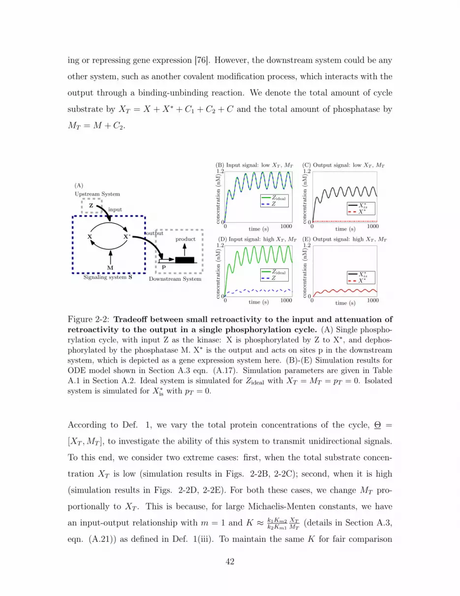
2-2 Tradeoff between small retroactivity to the input and attenuation

of retroactivity to the output in a single phosphorylation cycle. (A)

Single phosphorylation cycle, with input Z as the kinase: X is phosphorylated

by Z to X*, and dephosphorylated by the phosphatase M. X* is the output

and acts on sites p in the downstream system, which is depicted as a gene

expression system here. (B)-(E) Simulation results for ODE model shown

in Section A.3 eqn. (A.17). Simulation parameters are given in Table A.1 in

Section A.2. Ideal system is simulated for 𝑍ideal with 𝑋𝑇 = 𝑀𝑇 = 𝑝𝑇 = 0.

Isolated system is simulated for 𝑋*is with 𝑝𝑇 = 0. . . . . . . . . . . . . . 42

4-1 Procedure to determine if a given signaling system satisfies Def. 1

for unidirectional signal transmission. . . . . . . . . . . . . . . . . 52


of retroactivity to the output in a double phosphorylation cycle.

(A) Double phosphorylation cycle, with input Z as the kinase: X is phospho-

rylated by Z to X*, and further on to X**. Both these are dephosphorylated

by the phosphatase M. X** is the output and acts on sites p in the down-

stream system, which is depicted as a gene expression system here. (B)-(E)

Simulation results for ODE model (A.29) shown in Section A.4. Simulation

parameters are given in Table A.1 in Section A.2. The ideal system is sim-

ulated for 𝑍ideal with 𝑋𝑇 = 𝑀𝑇 = 𝑝𝑇 = 0. The isolated system for 𝑋**𝑖𝑠 is

simulated with 𝑝𝑇 = 0. . . . . . . . . . . . . . . . . . . . . . . . . . . 53

12


of retroactivity to the output in a phosphotransfer system. (A)

System with phosphorylation followed by phosphotransfer, with input Z as

the kinase: Z phosphorylates X1 to X*1. The phosphate group is transferred

from X*1 to X2 by a phosphotransfer reaction, forming X*2, which is in turn

dephosphorylated by the phosphatase M. X*2 is the output and acts on sites

p in the downstream system, which is depicted as a gene expression system

here. (B)-(E) Simulation results for ODE (A.49) in Section A.5. Simulation

parameters are given in Table A.1 in Section A.2. Ideal system is simulated

for 𝑍ideal with 𝑋𝑇1 = 𝑋𝑇2 = 𝑀𝑇 = 𝑝𝑇 = 0. Isolated system is simulated for

𝑋*2,𝑖𝑠 with 𝑝𝑇 = 0. . . . . . . . . . . . . . . . . . . . . . . . . . . . . . 55


of retroactivity to the output is overcome by a cascade of single

phosphorylation cycles. (A) Cascade of 2 phosphorylation cycles that

with kinase Z as the input: Z phosphorylates X1 to X*1, X*1 acts as the kinase

for X2, phosphorylating it to X*2, which is the output, acting on sites p in

the downstream system, which is depicted as a gene expression system here.

X*1 and X*2 are dephosphorylated by phosphatases M1 and M2, respectively.

(B), (C) Simulation results for ODEs (A.69)-(A.86) in Section A.7 with N

= 2. Simulation parameters are given in Table A.1 in Section A.2. Ideal

system is simulated for 𝑍ideal with 𝑋𝑇1 = 𝑋𝑇2 = 𝑀𝑇 = 𝑝𝑇 = 0. Isolated

system is simulated for 𝑋*2,𝑖𝑠 with 𝑝𝑇 = 0. . . . . . . . . . . . . . . . . . 58

13

4-5 Attenuation of retroactivity to the output by a phosphotransfer

system. (A) System with autophosphorylation followed by phosphotransfer,

with input as protein X1 which autophosphorylates to X*1. The phosphate

group is transferred from X*1 to X2 by a phosphotransfer reaction, forming

X*2, which is in turn dephosphorylated by the phosphatase M. X*2 is the

output and acts on sites p in the downstream system, which is depicted as

a gene expression system here. (B)-(E) Simulation results for ODE (A.99)

in Section A.8. Simulation parameters are given in Table A.1 in Section

A.2. Ideal system is simulated for 𝑋1,ideal with 𝑋𝑇2 = 𝑀𝑇 = 𝜋1 = 𝑝𝑇 = 0.

Isolated system is simulated for 𝑋*2,𝑖𝑠 with 𝑝𝑇 = 0. . . . . . . . . . . . . . 62

4-6 Inability to attenuate retroactivity to the output or impart small

retroactivity to the input by single phosphorylation cycle with

substrate as input. (A) Single phosphorylation cycle, with input X as the

substrate: X is phosphorylated by the kinase Z to X*, which is dephospho-

rylated by the phosphatase M back to X. X* is the output and acts as a

transcription factor for the promoter sites p in the downstream system. (B)-

(E) Simulation results for ODEs (A.110),(A.111) in Section A.9. Simulation

parameters are given in Table A.1 in Section A.2. Ideal system is simulated

for 𝑋ideal with 𝑍𝑇 = 𝑀𝑇 = 𝑝𝑇 = 0. Isolated system is simulated for 𝑋*is

with 𝑝𝑇 = 0. . . . . . . . . . . . . . . . . . . . . . . . . . . . . . . . . 64

14

4-7 Table summarizing the results. For each inset table, a X(7) for column

𝑟 implies the system can (cannot) be designed to minimize retroactivity

to the input by varying total protein concentrations, a X(7) for column 𝑠

implies the system can (cannot) be designed to attenuate retroactivity to

the output by varying total protein concentrations, column 𝑚 describes the

input-output relationship of the system (i.e., 𝑌 ≈ 𝐾𝑈𝑚) as described in

Def. 1(iii). Inset tables with two rows imply that one of the two rows can

be achieved for a set of values for the design parameters: thus, the two

rows for systems (A), (B) and (C) show the trade-off between the ability to

minimize retroactivity to the input (first row) and the ability to attenuate

retroactivity to the output (second row). Note that this trade-off is overcome

by the cascade (E). . . . . . . . . . . . . . . . . . . . . . . . . . . . . 67

6-1 Examples of network motifs found in GRNs involved in cell fate determina-

tion. Here, arrows “→" represent activation (positive interaction) and arrows

“–|" represent repression (negative interaction). (a) Mutual antagonism net-

work, where two nodes mutually repress one another while self-activating.

(b) Two-node mutual cooperation network, where two nodes mutually acti-

vate one another while also self-activating. (c) Three-node mutual coopera-

tion network, where each node activates the others and itself. . . . . . . . 73

15

6-2 Nullclines of the ODEs modeling the two-node network motifs

given by (6.1), (6.2), (6.3) when unstimulated (𝑤 = 0). Filled circles

represent the stable steady states 𝑆1, 𝑆2 and 𝑆3. Blue arrows show vector

field (1, 2). Regions of attraction of the stable steady states 𝑆1, 𝑆2 and

𝑆3 are shown by the coral, blue and purple shaded regions, respectively. (a)

Nullclines for the system of ODEs modeling the mutual antagonism net-

work, with ℎ𝑖(𝑥) given by (6.2). Parameters: 𝛼1 = 5nMs−1, 𝛽1 = 3nMs−1,

𝛼2 = 5.2nMs−1, 𝛽2 = 4nMs−1, 𝑛1 = 𝑛2 = 𝑛3 = 𝑛4 = 2, 𝑘1 = 𝑘2 = 1nM,

𝛾1 = 𝛾2 = 0.2s−1. (b) Nullclines for the system of ODEs modeling the two-

node mutual cooperation network, with ℎ𝑖(𝑥) given by (6.3). Parameters:

𝜂1 = 𝜂2 = 10−4nMs−1, 𝑎1 = 2nMs−1, 𝑏1 = 0.25nMs−1, 𝑐1 = 2.5nMs−1,

𝑎2 = 0.18nMs−1, 𝑏2 = 2nMs−1, 𝑐2 = 2.5nMs−1, 𝑛1 = 𝑛2 = 𝑛3 = 2,

𝑘1 = 𝑘2 = 𝑘3 = 1nM, 𝛾1 = 𝛾2 = 1s−1. . . . . . . . . . . . . . . . . . . . 74

7-1 Reprogramming to a desired stable steady state 𝑆𝑑. The red dashed

arrow represents the trajectory of the stimulated system Σ𝑤 and blue solid

arrow represents the trajectory of the unstimulated system Σ0. The stim-

ulated system Σ𝑤 has an asymptotically stable steady state 𝑥𝑑 such that

lim𝑡→∞ 𝜑𝑤(𝑡, 𝑥0) = 𝑥𝑑, and 𝑥𝑑 ∈ ℛ0(𝑆𝑑) so that the system Σ0 is repro-

grammed to 𝑆𝑑 under input 𝑤. . . . . . . . . . . . . . . . . . . . . . . 80

16

8-1 Inputs of type 1 and 2 applied to the two-node networks of mutual

antagonism and mutual cooperation as in (6.1). Resulting vector fields

and stable steady states of the stimulated system Σ𝑤 are shown via red

arrows and solid red circles, respectively. The regions of attraction of 𝑆1, 𝑆2

and 𝑆3 (solid black circles) for the unstimulated system Σ0 are shown in the

background in coral, blue and purple, respectively. (a) An input of type 1,

with 𝑢1 = 3nMs−1, 𝑣2 = 10s−1 is applied to the mutual antagonism network.

This results in a globally asymptotically stable steady state in the region of

attraction of 𝑆3, and thus the input of type 1 strongly reprograms the system

to the maximum steady state 𝑆3. (b) An input of type 2, with 𝑣1 = 10s−1,

𝑢2 = 2nMs−1 is applied to mutual antagonism network. This results in a

globally asymptotically stable steady state in the region of attraction of 𝑆1,

and thus the input of type 2 strongly reprograms the system to the minimum

steady state 𝑆1. (c) An input of type 1, with 𝑢1 = 2nMs−1, 𝑢2 = 1.8nMs−1

is applied to the mutual cooperation network. This results in a globally

asymptotically stable steady state in the region of attraction of 𝑆3, and thus

the input of type 1 strongly reprograms the system to the maximum steady

state 𝑆3. (d) An input of type 2, with 𝑣1 = 4s−1, 𝑣2 = 6s−1 is applied to

the mutual cooperation network. This results in a globally asymptotically

stable steady state in the region of attraction of 𝑆1, and thus the input of

type 2 strongly reprograms the system to the minimum steady state 𝑆1. . 85

9-1 Input of type 1 applied to the network of mutual cooperation to

attempt to weakly reprogram it from 𝑆1 to 𝑆2 (big black circles).

Increasing 𝑢1 and/or 𝑢2 (the positive input on nodes x1 and x2, respectively)

changes the shape of the nullclines 1 = 0 and/or 2 = 0 such that the stable

steady state in the blue region (ℛ0(𝑆2)) disappears before the stable steady

state 𝑎*(𝑤) (small red circles) in the coral region (ℛ0(𝑆1)). Finally, for large

𝑢1 and/or large 𝑢2, only a stable steady state in the purple region (ℛ0(𝑆3))

remains. . . . . . . . . . . . . . . . . . . . . . . . . . . . . . . . . . . 88

17

9-2 Inputs of type 3 applied to the two-node network of mutual antag-

onism as in (6.1). Resulting vector fields and stable steady states of the

stimulated system are shown in red. The regions of attraction of 𝑆1, 𝑆2 and

𝑆3 for the unstimulated system Σ0 are shown in the background in coral,

blue and purple, respectively. (a) An input of type 3, with 𝑢1 = 3nMs−1,

𝑢2 = 2nMs−1 is applied to the mutual antagonism network. The resulting

globally asymptotically stable steady state is in the region of attraction of

𝑆2, and thus the input of type 3 strongly reprograms the system to the inter-

mediate steady state 𝑆2. (b) An input of type 3, with 𝑣1 = 8s−1, 𝑣2 = 12s−1

is applied to the mutual antagonism network. This results in a globally

asymptotically stable steady state in the region of attraction of 𝑆2, and thus

this input of type 3 strongly reprograms the system to the steady state 𝑆2. 90

9-3 The set 𝑊𝑖 defined in (9.1) shown by the bold black lines. . . . . . . 91

18

9-4 Iteratively discretizing [0, 1]2 to find the input parameter ′ such that the

input tuple (𝑤′, 𝑇1, 𝑇2) strongly 𝜖-reprogram the system to 𝑆2, where 𝑇1

and 𝑇2 are fixed. We have 𝑛 = 2, 𝑢𝑚1 = 100nMs−1, 𝑢𝑚2 = 30nMs−1,

𝑣𝑚1 = 𝑣𝑚2 = 3s−1, 𝑆𝑑 = 𝑆2, 𝑚 = (0, 0), S = 𝑆1, 𝑆2, 𝑆3, 𝜖 = 0.01.

Initial guesses 𝑇1 = 1000s, 𝑇2 = 1000s, 𝑁max = 4. (a) Discretization with

𝑟 = 1. Inputs 𝑤 corresponding to grid-points (marked by filled black

circles) reprogram the system to the steady states marked at the corners.

(b) Discretization with 𝑟 = 2. Previously tried grid-points are marked by

hollow circles, and new grid-points are marked by filled circles. Steady states

to which inputs corresponding to these grid-points 𝜖-reprogram the system

are labeled next to each corner. (c) Grey area denotes the region between

any two input pairs in elim at that iteration. The space is discretized using

𝑟 = 4, grid-points not in the eliminated regions are tried, and steady states to

which inputs corresponding to grid-points reprogram the system are marked

in the figure. (d) Similar to (c), the grey area denotes the regions between

any two input pairs in elim at that iteration. We find that grid-point (circled

in red) 𝑑 = (0.125, 0) is such that input 𝑤𝑑 is the solution. From (9.3), we

have 𝑤𝑑1 = (𝑢𝑚1/4, 𝑣𝑚1), 𝑤𝑑2 = (0, 𝑣𝑚2). Input tuple (𝑤𝑑, 𝑇1, 𝑇2) is found

to 𝜖-reprogram the system to the desired steady state 𝑆2. . . . . . . . . . 102

9-5 Strongly 𝜖-reprogramming two-node mutual cooperation network to its in-

termediate stable steady state 𝑆2, using input tuple (𝑤𝑑, 𝑇1, 𝑇2), where

𝑤𝑑 = (𝑤𝑑1, 𝑤𝑑2), 𝑤𝑑1 = (25nMs−1, 3s−1), 𝑤𝑑2 = (0, 3s−1), 𝑇1 = 1000s,

𝑇2 = 1000s. (a) System Σ𝑤𝑑is simulated for time 𝑇1, starting at initial

conditions 𝑥0 ∈ 𝑆1, 𝑆2, 𝑆3. Resulting trajectories are shown in red, and

end-points of trajectories 𝜑𝑤𝑑(𝑇1, 𝑥

0) are shown by solid red dots. In this

case, all three end-points closely coincide with the globally asymptotically

stable steady state of Σ𝑤𝑑. (b) System Σ0 is simulated for time 𝑇2, start-

ing at initial conditions 𝜑𝑤𝑑(𝑇1, 𝑥

0) for all 𝑥0 ∈ 𝑆1, 𝑆2, 𝑆3. After 𝑇2, end

points of trajectories, 𝜑0(𝑇2, 𝜑𝑤𝑑(𝑇1, 𝑥

0)), are within an 𝜖 ball of 𝑆2 with

𝜖 = 10−3. . . . . . . . . . . . . . . . . . . . . . . . . . . . . . . . . . . 104

19

10-1 The extended pluripotency network. . . . . . . . . . . . . . . . . . . . 113

10-2 The core pluripotency network . . . . . . . . . . . . . . . . . . . . . . 115

10-3 Stable steady states of the core pluripotency network . . . . . . . . . 115

10-4 Stable steady-states and vector-field of the core pluripotency net-

work (10.2). Parameters of this system are: 𝜂1 = 𝜂2 = 𝜂3 = 10−4,

𝛾1 = 𝛾2 = 𝛾3 = 1, 𝑎1 = 1, 𝑏12 = 0.147, 𝑏13 = 0.073, 𝑐12 = 1.27, 𝑐13 = 0.63,

𝑑12 = 0.67, 𝑑13 = 0.34, 𝑒12 = 0.67, 𝑒13 = 0.34, 𝑎2 = 1.6, 𝑏21 = 0.14,

𝑏23 = 0.8, 𝑐21 = 4, 𝑑2 = 0.67, 𝑑21 = 1, 𝑑23 = 0.34, 𝑒21 = 1, 𝑎3 = 0.816,

𝑏31 = 0.143, 𝑏32 = 1.616, 𝑐31 = 4.08, 𝑑3 = 0.34, 𝑑31 = 1, 𝑑32 = 0.67, 𝑒31 = 1.

For this set of parameters, the system has three stable steady states 𝑆𝑚𝑖𝑛,

𝑆𝑖𝑛𝑡 and 𝑆𝑚𝑎𝑥, shown by black dots. The vector field (1, 2, 3) is shown

by the blue arrows, and is normalized for visualization. . . . . . . . . . . 116

10-5 Input of type 1 applied to the core pluripotency network. A suffi-

ciently large input of type 1 is used to strongly reprogram the 3-node mutual

cooperation network to its maximum steady state 𝑆𝑚𝑎𝑥. (a) A sufficiently

large input of type 1, in this case 𝑤 such that 𝑤1 = (2, 0), 𝑤2 = (2, 0),

𝑤3 = (2, 0) results in a globally exponentially stable steady state, shown by

the solid red dot. (b) The globally exponentially stable steady state of the

stimulated system is in the region of attraction of 𝑆𝑚𝑎𝑥, and once the input

is removed, the unstimualted system converges to 𝑆𝑚𝑎𝑥. . . . . . . . . . . 117

10-6 Input of type 2 applied to the core pluripotency network. A suffi-

ciently large input of type 2 is used to strongly reprogram the 3-node mutual

cooperation network to its maximum steady state 𝑆𝑚𝑖𝑛. (a) A sufficiently

large input of type 1, in this case 𝑤 such that 𝑤1 = (0, 5), 𝑤2 = (0, 5),

𝑤3 = (0, 5) results in a globally exponentially stable steady state, shown by

the solid red dot. (b) The globally exponentially stable steady state of the

stimulated system is in the region of attraction of 𝑆𝑚𝑖𝑛, and once the input

is removed, the unstimualted system converges to 𝑆𝑚𝑖𝑛. . . . . . . . . . . 117

20

10-7 Input tuple strongly 𝜖-reprograms the core pluripotency network

to 𝑆𝑖𝑛𝑡. The search procedure outlined in Section 9.3 is used to find an

input tuple that 𝜖-reprograms the network to the intermediate stable steady

state 𝑆𝑖𝑛𝑡. The procedure is initialized with 𝑛 = 3, 𝑢𝑚1 = 𝑢𝑚2 = 𝑢𝑚3 = 24,

𝑣𝑚1 = 𝑣𝑚2 = 𝑣𝑚3 = 3, 𝑆𝑑 = 𝑆𝑖𝑛𝑡, 𝑚 = (0, 0, 0), S = 𝑆𝑚𝑎𝑥, 𝑆𝑚𝑖𝑛, 𝑆𝑖𝑛𝑡,

𝜖 = 0.01. We run the procedure with two sets of guesses. The first set is

picked arbitrarily with 𝑇1 = 1, 𝑇2 = 1 and 𝑁max = 1. This procedure tries

a total of 165 input tuples, before finding a solution (𝑤𝑑, 𝑇1, 𝑇2) with 𝑤𝑑1 =

(𝑢𝑚1/8, 𝑣𝑚1), 𝑤𝑑2 = (0, 𝑣𝑚1), 𝑤𝑑3 = (0, 𝑣𝑚3), and 𝑇1 = 𝑇2 = 1000000s.

Without the elimination condition, the procedure tries a total of 1632 input

tuples. (a) The input 𝑤𝑑 is applied to the network as in (6.1) for time

𝑇1 = 1000000s. The end points of the trajectories starting at 𝑆𝑚𝑎𝑥, 𝑆𝑚𝑖𝑛,

and 𝑆𝑚𝑎𝑥 are close to the globally exponentially stable steady state of the

stimulated system. (b) The input is removed, and the unstimulated system

is simulated for time 𝑇2 = 1000000s. The system converges 𝜖-close to desired

steady state 𝑆𝑖𝑛𝑡. . . . . . . . . . . . . . . . . . . . . . . . . . . . . . 119

10-8 Reprogramming the system to the pluripotent stem cell state, using inputs

that reprogram the core network to 𝑆𝑖𝑛𝑡. . . . . . . . . . . . . . . . . . 124

A-1 Tradeoff between small retroactivity to the input and attenuation

of retroactivity to the output in a single phosphorylation cycle. (A)

Single phosphorylation cycle, with input Z as the kinase: X is phosphorylated

by Z to X*, and dephosphorylated by the phosphatase M. X* is the output


expression system here. (B)-(E) Simulation results for ODE model shown in

SI Section A.3 eqn. (A.17). Simulation parameters are given in Table A.1 in

SI Section A.2. Ideal system is simulated for 𝑍ideal with 𝑋𝑇 = 𝑀𝑇 = 𝑝𝑇 = 0.

Isolated system is simulated for 𝑋*is with 𝑝𝑇 = 0. . . . . . . . . . . . . . 139

21


of retroactivity to the output in a double phosphorylation cycle.

(A) Double phosphorylation cycle, with input Z as the kinase: X is phospho-

rylated by Z to X*, and further on to X**. Both these are dephosphorylated

by the phosphatase M. X** is the output and acts on sites p in the down-

stream system, which is depicted as a gene expression system here. (B)-(E)

Simulation results for ODE model (A.29) shown in SI Section A.4. Simula-

tion parameters are given in Table A.1 in SI Section A.2. The ideal system

is simulated for 𝑍ideal with 𝑋𝑇 = 𝑀𝑇 = 𝑝𝑇 = 0. The isolated system for

𝑋**𝑖𝑠 is simulated with 𝑝𝑇 = 0. . . . . . . . . . . . . . . . . . . . . . . . 144


of retroactivity to the output in a phosphotransfer system. (A)

System with phosphorylation followed by phosphotransfer, with input Z as

the kinase: Z phosphorylates X1 to X*1. The phosphate group is transferred

from X*1 to X2 by a phosphotransfer reaction, forming X*2, which is in turn

dephosphorylated by the phosphatase M. X*2 is the output and acts on sites


here. (B)-(E) Simulation results for ODE (A.49) in SI Section A.5. Simu-

lation parameters are given in Table A.1 in SI Section A.2. Ideal system is

simulated for 𝑍ideal with 𝑋𝑇1 = 𝑋𝑇2 = 𝑀𝑇 = 𝑝𝑇 = 0. Isolated system is

simulated for 𝑋*2,𝑖𝑠 with 𝑝𝑇 = 0. . . . . . . . . . . . . . . . . . . . . . . 150

22


of retroactivity to the output is overcome by a cascade of single

phosphorylation cycles. (A) Cascade of 2 phosphorylation cycles that

with kinase Z as the input: Z phosphorylates X1 to X*1, X*1 acts as the kinase

for X2, phosphorylating it to X*2, which is the output, acting on sites p in

the downstream system, which is depicted as a gene expression system here.

X*1 and X*2 are dephosphorylated by phosphatases M1 and M2, respectively.

(B), (C) Simulation results for ODEs (A.69)-(A.86) in SI Section A.7 with N

= 2. Simulation parameters are given in Table A.1 in SI Section A.2. Ideal

system is simulated for 𝑍ideal with 𝑋𝑇1 = 𝑋𝑇2 = 𝑀𝑇 = 𝑝𝑇 = 0. Isolated

system is simulated for 𝑋*2,𝑖𝑠 with 𝑝𝑇 = 0. . . . . . . . . . . . . . . . . . 155

A-5 Figures showing the variation of 𝜖3 with 𝑁 , for different 𝑋𝑇𝑁 . Parameter

values are: 𝐾𝑚1 = 𝐾𝑚2 = 300𝑛𝑀 , 𝑘1 = 𝑘2 = 600𝑠−1, 𝜆 = 1, (a) 𝑋𝑇𝑁 =

1000𝑛𝑀 , where resulting = 6 and (b) 𝑋𝑇𝑁 = 10000𝑛𝑀 , where resulting

= 8. . . . . . . . . . . . . . . . . . . . . . . . . . . . . . . . . . . . 166

23

A-6 Tradeoff between small retroactivity to the input and attenuation of retroac-

tivity to the output is overcome by a cascade of a phosphotransfer system

with a single phosphorylation cycle. (A) Cascade of a phosphotransfer sys-

tem that receives its input through a kinase Z phosphorylating the phosphate

donor, and a phosphorylation cycle: Z phosphorylates X1 to X*1, X*1 transfers

the phosphate group in a reversible reaction to X2. X*2 further acts as the

kinase for X3, phosphorylating it to X*3, which is the output, acting on sites


here. Both X*2 and X*3 are dephosphorylated by phosphatase M. (B), (C)

Simulation results for ODE model (A.91),(A.92). Simulation parameters:

𝑘(𝑡) = 0.01(1 + 𝑠𝑖𝑛(0.05𝑡))𝑛𝑀.𝑠−1, 𝛿 = 0.01𝑠−1, 𝑎1 = 𝑎2 = 𝑑3 = 𝑎4 = 𝑎5 =

𝑎6 = 18𝑛𝑀−1𝑠−1, 𝑑1 = 𝑑2 = 𝑎3 = 𝑑4 = 𝑑5 = 𝑑6 = 2400𝑠−1, 𝑘1 = 𝑘4 = 𝑘5 =

𝑘6 = 600𝑠−1. (B) Effect of retroactivity to the input: for the ideal input

𝑍ideal, system is simulated with 𝑋𝑇1 = 𝑋𝑇2 = 𝑋𝑇3 = 𝑀𝑇 = 𝑝𝑇 = 0; for

actual input 𝑍, system is simulated with 𝑋𝑇1 = 3𝑛𝑀 , 𝑋𝑇2 = 1200𝑛𝑀 ,

𝑋𝑇3 = 1200𝑛𝑀 , 𝑀𝑇 = 3𝑛𝑀, 𝑝𝑇 = 100𝑛𝑀 . (C) Effect of retroactiv-

ity to the output: for the isolated output 𝑋*3,is, system is simulated with

𝑋𝑇1 = 3𝑛𝑀 , 𝑋𝑇2 = 1200𝑛𝑀 , 𝑋𝑇3 = 1200𝑛𝑀 , 𝑀𝑇 = 3𝑛𝑀, 𝑝𝑇 = 0; for the

actual output 𝑋*3 , system is simulated with 𝑋𝑇1 = 3𝑛𝑀 , 𝑋𝑇2 = 1200𝑛𝑀 ,

𝑋𝑇3 = 1200𝑛𝑀 , 𝑀𝑇 = 3𝑛𝑀, 𝑝𝑇 = 100𝑛𝑀 . . . . . . . . . . . . . . . . . 167

24

A-7 Tradeoff between small retroactivity to the input and attenuation of retroac-

tivity to the output is overcome by a cascade of a single phosphorylation cycle

and a double phosphorylation cycle. (A) Cascade of a a single phosphoryla-

tion and a double phosphorylation cycle with input kinase Z: Z phosphory-

lates X1 to X*1, X*1 further acts as the kinase for X2, phosphorylating it to

X*2 and X**2 , which is the output, acting on sites p in the downstream sys-

tem, which is depicted as a gene expression system here. All phosphorylated

proteins X*1, X*2 and X**2 are dephosphorylated by phosphatase M. (B), (C)

Simulation results for ODE model (A.93), (A.94). Simulation parameters:

𝑘(𝑡) = 0.01(1 + 𝑠𝑖𝑛(0.05𝑡))𝑛𝑀.𝑠−1, 𝛿 = 0.01𝑠−1, 𝑎1 = 𝑎2 = 𝑎3 = 𝑎4 = 𝑎5 =

𝑎6 = 18𝑛𝑀−1𝑠−1, 𝑑1 = 𝑑2 = 𝑑3 = 𝑑4 = 𝑑5 = 𝑑6 = 2400𝑠−1, 𝑘1 = 𝑘2 = 𝑘3 =

𝑘4 = 𝑘5 = 𝑘6 = 600𝑠−1. (B) Effect of retroactivity to the input: for the ideal

input 𝑍ideal, system is simulated with 𝑋𝑇1 = 𝑋𝑇2 = 𝑋𝑇3 = 𝑀𝑇 = 𝑝𝑇 = 0;

for actual input 𝑍, system is simulated with 𝑋𝑇1 = 3𝑛𝑀 , 𝑋𝑇2 = 1200𝑛𝑀 ,

𝑀𝑇 = 9𝑛𝑀, 𝑝𝑇 = 100𝑛𝑀 . (C) Effect of retroactivity to the output: for

the isolated output 𝑋*2,is, system is simulated with 𝑋𝑇1 = 3𝑛𝑀 , 𝑋𝑇2 =

1200𝑛𝑀 , 𝑀𝑇 = 9𝑛𝑀, 𝑝𝑇 = 0; for the actual output 𝑋*2 , system is simulated

with 𝑋𝑇1 = 3𝑛𝑀 , 𝑋𝑇2 = 1200𝑛𝑀 , 𝑀𝑇 = 9𝑛𝑀, 𝑝𝑇 = 100𝑛𝑀 . . . . . . . 169

A-8 Attenuation of retroactivity to the output by a phosphotransfer

system. (A) System with autophosphorylation followed by phosphotransfer,

with input as protein X1 which autophosphorylates to X*1. The phosphate

group is transferred from X*1 to X2 by a phosphotransfer reaction, forming

X*2, which is in turn dephosphorylated by the phosphatase M. X*2 is the

output and acts on sites p in the downstream system, which is depicted as a

gene expression system here. (B)-(E) Simulation results for ODE (A.99) in

SI Section A.8. Simulation parameters are given in Table A.1 in SI Section

A.2. Ideal system is simulated for 𝑋1,ideal with 𝑋𝑇2 = 𝑀𝑇 = 𝜋1 = 𝑝𝑇 = 0.

Isolated system is simulated for 𝑋*2,𝑖𝑠 with 𝑝𝑇 = 0. . . . . . . . . . . . . . 170

25

A-9 Inability to attenuate retroactivity to the output or impart small

retroactivity to the input by single phosphorylation cycle with

substrate as input. (A) Single phosphorylation cycle, with input X as

the substrate: X is phosphorylated by the kinase Z to X*, which is dephos-

phorylated by the phosphatase M back to X. X* is the output and acts as

a transcription factor for the promoter sites p in the downstream system.

(B)-(E) Simulation results for ODEs (A.110),(A.111) in SI Section A.9. Sim-

ulation parameters are given in Table A.1 in SI Section A.2. Ideal system is

simulated for 𝑋ideal with 𝑍𝑇 = 𝑀𝑇 = 𝑝𝑇 = 0. Isolated system is simulated

for 𝑋*is with 𝑝𝑇 = 0. . . . . . . . . . . . . . . . . . . . . . . . . . . . . 175


retroactivity to the input by double phosphorylation cycle with

substrate as input. (A) Double phosphorylation cycle, with input X as

the substrate: X is phosphorylated twice by the kinase K to X* and X**,

which are in turn dephosphorylated by the phosphatase M. X** is the output


expression system here. (B)-(E) Simulation results for ODE (A.124) in SI

Section A.10. Simulation parameters are given in Table A.1 in SI Section

A.2. Ideal system is simulated for 𝑋ideal with 𝑍𝑇 = 𝑀𝑇 = 𝑝𝑇 = 0. Isolated

system is simulated for 𝑋**𝑖𝑠 with 𝑝𝑇 = 0. . . . . . . . . . . . . . . . . . . 179


retroactivity to the input by double phosphorylation cycle with

substrate as input. (A) Double phosphorylation cycle, with input X as

the substrate: X is phosphorylated twice by the kinase K to X* and X**,

which are in turn dephosphorylated by the phosphatase M. X** is the output


expression system here. (B)-(E) Simulation results for ODE (A.124) in SI

Section A.10. Simulation parameters are given in Table A.1 in SI Section

A.2. Ideal system is simulated for 𝑋ideal with 𝑍𝑇 = 𝑀𝑇 = 𝑝𝑇 = 0. Isolated

system is simulated for 𝑋**𝑖𝑠 with 𝑝𝑇 = 0. . . . . . . . . . . . . . . . . . . 180

26

List of Tables

10.1 Stable steady states of the extended pluripotency network. The

parameters of the core network are the same as those in Section 10.2.1. The

rest of the parameters of the system are: 𝑑25 = 1.5, 𝑑24 = 0.01, 𝜂4 = 𝜂5 = 4,

𝑑42 = 242.6, 𝑑51 = 0.98, 𝛾4 = 1, 𝛾5 = 10. . . . . . . . . . . . . . . . . . . 122

A.1 Table of simulation parameters for Figures 2-2, 4-2-4-6, A-1-A-4, A-8-

A-11. . . . . . . . . . . . . . . . . . . . . . . . . . . . . . . . . . . . . 138

A.2 System variables, functions and matrices for a double phosphorylation

cycle with the kinase for both cycles as input brought to form (3.1). . 141


cycle with the kinase for both cycles as input brought to form (3.1). . 146

A.4 System variables, functions and matrices for a phosphotransfer system

with kinase as input brought to form (3.1). . . . . . . . . . . . . . . . 152

A.5 System variables, functions and matrices for a cascade of two phospho-

rylation cycles with kinase as input brought to form (3.1). . . . . . . 157

A.6 System variables, functions and matrices for an N-stage cascade of

phosphorylation cycles with the kinase as input to the first cycle brought

to form (3.1). . . . . . . . . . . . . . . . . . . . . . . . . . . . . . . . 163

A.7 System variables, functions and matrices for a phosphotransfer system

with autophosphorylation brought to form (3.1). . . . . . . . . . . . . 172

A.8 System variables, functions and matrices for a single phosphorylation

cycle with substrate as input brought to form (3.1). . . . . . . . . . . 177

27


cycle with substrate as input brought to form (3.1). . . . . . . . . . . 182

28

Chapter 1

Introduction

Biomolecular reaction networks allow cells to sense, remember and respond to external

stimuli. In these networks, information travels through processes such as production,

modification, and removal of biomolecules. These processes can be modeled mech-

anistically by means of ordinary differential equations, and these networks can be

treated as input-output systems, where the input, output and state variables are con-

centrations of the biomolecules involved in these reactions. In this thesis, we study

two key biomolecular networks. In the first part, we study signaling systems, which

are responsible for transmitting information from one process in the cell (such as a

sensor on the cell wall) to another (such as a gene regulatory network controlling the

cell’s response to the stimulus). These signaling systems transmit information to gene

regulatory networks, which are responsible for controlling several cellular functions.

In the second part of the thesis, we focus on gene regulatory networks controlling one

key cellular function – cellular differentiation, which is the process in which a cell

changes from one cell type to another.

1.1 Motivation

Signaling systems are the biomolecular reactions that allow cells to detect and process

changes in their environment, as well as enable intra- and inter-cellular comminica-

tion. For example, the signaling pathway characterized in [1] is activated by a growth

29

factor and once activated, shuts down proteins facilitating cell-death. Cellular sig-

nal transduction is typically viewed as a unidirectional transmission of information

(Fig. 1-1A) via biochemical reactions from an upstream system to multiple down-

stream systems through signaling pathways [2]-[7]. However, without the presence of

specialized mechanisms, signal transmission via chemical reactions is not in general

unidirectional. In fact, the chemical reactions that allow a signal to be transmitted

from an upstream system to downstream systems also affect the dynamics of the up-

stream system. This back-effect is called retroactivity (Fig. 1-1B).

While retroactivity effects have been shown to be useful in certain contexts, such

as transcription factor decoy sites that convert graded dose-responses to sharper,

more switch-like responses [8], retroactivity is one of the chief hurdles to one-way

transmission of information [9]-[14]. Signaling pathways, typically composed of phos-

phorylation, dephosphorylation and phosphotransfer reactions, are highly conserved

evolutionarily, such as the MAPK cascade [15] and two-component signaling sys-

tems [16]. Thus, the same pathways act between different upstream and downstream

systems in different scenarios and organisms, facing different effects of retroactivity

in different contexts. For signal transmission to be unidirectional in these differ-

ent contexts, a signaling pathway should have evolved architectures that overcome

retroactivity. Specifically, these architectures should impart a small retroactivity to

their upstream system (called retroactivity to the input – ℛ in Fig. 1-1B) and should

be minimally affected by the retroactivity imparted to them by their downstream

systems (retroactivity to the output – 𝒮 in Fig. 1-1B).

Phosphorylation-dephosphorylation cycles, phosphotransfer reactions, and cascades

of these are ubiquitous in both prokaryotic and eukaryotic signaling pathways, playing

a major role in cell cycle progression, survival, growth, differentiation and apoptosis

[2]-[7], [17]-[20]. Numerous studies have been conducted to analyze such systems,

starting with milestone works by Stadtman and Chock [21], [22], [23] and Goldbeter

et al. [24], [25], [26], which theoretically and experimentally analyzed phosphoryla-

30

UpstreamSystem

DownstreamSystem

U YSignalingsystem

(A)

UpstreamSystem

DownstreamSystem

U Y

R S

Signalingsystem

(B)

Figure 1-1: Signaling systems transmit information from an upstream system toa downstream system. (A) A signaling system transmitting information unidirectionally:𝑈 is the input from the upstream system to the signaling system. 𝑌 is the output of thesignaling system, sent to the downstream system. (B) Retroactivity is the back-effect fromdownstream systems to the upstream system: R is the retroactivity signal from the signalingsystem to the upstream system (retroactivity to the input of the signaling system), and S isthe retroactivity signal from the downstream system to the signaling system (retroactivityto the output of the signaling system).

tion cycles and cascades. These systems were further investigated by Kholdenko et al.

[27], [28], [29] and Gomez-Uribe et al. [30], [31]. However, these studies considered

signaling cycles in isolation, and thus did not investigate the effect of retroactivity.

The effect of retroactivity on such systems was theoretically analyzed in the work

by Ventura et al. [32], where retroactivity is treated as a “hidden feedback" to the

upstream system. Experimental studies then confirmed the effects of retroactivity in

signaling systems through in vivo experiments on the MAPK cascade [13], [14] and

in vitro experiments on reconstituted covalent modification cycles [10], [12]. These

studies clearly demonstrated that the effects of retroactivity on a signaling system

manifest themselves in two ways: (1) it causes a slow down of the temporal response

of the signaling system’s output to its input, and (2) it leads to a change of the out-

put’s steady state.

In 2008, Del Vecchio et al. demonstrated theoretically that a single phosphorylation-

dephosphorylation (PD) cycle with a slow input kinase can attenuate the effect of

retroactivity to the output when the total substrate and phosphatase concentrations

of the cycle are increased together [9]. Essentially, a sufficiently large phosphatase

31

concentration along with relatively large kinetic rates of modification adjusts the cy-

cle’s internal dynamics very quickly with respect to a relatively slower input, making

any retroactivity-induced delays negligible on the time scale of the signal being trans-

mitted [33]. A similarly large concentration of total cycle’s substrate ensures that the

output’s steady state is not significantly affected by the presence of downstream sites.

These theoretical findings were later verified experimentally both in vitro [12] and in

vivo [34]. Although a single PD cycle can attenuate the effect of retroactivity to the

output, it is unfortunately unsuitable for unidirectional signal transmission. In fact,

as the substrate concentration is increased, the PD cycle applies a large retroactivity

to the input, causing the input signal to slow down. This was experimentally observed

in [34]. The experimental results of [35] further suggest that a cascade composed of

two PD cycles and a phosphotransfer reaction could overcome both retroactivity to

the input and retroactivity to the output. In [36], it was theoretically found that,

for certain parameter conditions, a cascade of PD cycles could attenuate the upward

(from downstream to upstream) propagation of disturbances applied downstream of

the cascade. In [37], a parametric study was performed on a cascade of single phospho-

rylation cycles at steady-state, and parametric regimes in which the cascade would

transmit signals either upstream (using retroactivity) or downstream were numeri-

cally determined. These results suggest that specific signaling architectures may be

able to counteract retroactivity. However, to the best of the authors’ knowledge, no

attempt has been made to systematically characterize signaling architectures with

respect to their ability to overcome the effects of retroactivity and therefore enable

unidirectional signal transmission. Such signaling architectures transmit information

within the cell, and trigger various gene regulatory networks. Architectures that do

enable unidirectional signal transmission can then be abstracted away as directional

edges in such networks, allowing for easier analysis of the GRNs. One of the chief

processes such GRNs control is the process of cellular differentiation, which is the

subject for the second part of the thesis.

The ancestry of every cell in an adult’s body can be traced back to the pluripotent

32

stem cells of the inner cell mass of the embryo, the “master" cells. For a long time,

cell differentiation was thought to be final and irreversible; once a cell became special-

ized, it could not revert back to a stage where it had the ability to differentiate into

multiple different cell types. Waddington’s epigenetic landscape analogy [38] views

different cellular phenotypes as local minima in the landscape, and the cell state as

a ball rolling downhill that either settles in these local minima or continues rolling

downhill [39, 40, 41]. The lowest basins in this landscape represent the terminally

differentiated cells. The ball cannot roll uphill, and this popular metaphor was used

to explain the concept that cellular differentiation is irreversible. This viewpoint was

demolished in 2006 by Shinya Yamanaka and co-workers [42]. “For the discovery that

terminally differentiated cells can be reprogrammed to become pluripotent", he won

the Nobel Prize along with Sir John Gordon in 2012. By over-expressing four key

transcription factors, they converted somatic cells into induced pluripotent stem cells

(iPSCs). This discovery, along with the first demonstration of transdifferentiation

(converting a mature somatic cell to another) in 2000 [43], revolutionized the fields

of biology and medicine, and created new research fields in its wake. Since then,

many successful attempts at reprogramming cell fate, that is, artificially converting

cells from one phenotype to another using external inputs, have been seen: pancreatic

exocrine cells into 𝛽-cells [44], fibroblasts into neurons [45, 46], fibroblasts into hep-

atocytes [47], hepatocytes into functional insulin-producing cells [48], and fibroblasts

into neural progenitors [49], among others. These processes of cell fate conversion

have potential applications in disease modeling, drug discovery, gene therapy, and

regenerative medicine.

The above cell fate conversion processes all involve the application of external (pos-

itive or negative) stimulations to select nodes of a gene regulatory network (GRN),

by increasing the rate of production of the transcription factor (TF) in the node

(most common approach) or by enhancing its degradation. However, selecting the

nodes where the input stimulation needs to be applied and the required stimulation

type (positive or negative) for triggering a desired state transition typically relies on

33

biological intuition and on trial-and-error experiments [44, 45, 47, 46]. These “in-

tuitive" inputs typically increase factors that are highly expressed in the target cell

with respect to the initial cell type and/or decrease factors that are low. It has been

theoretically shown in the case of reprogramming to pluripotent stem cells, that “in-

tuitive" inputs, such as up-regulating factors that are higher in the target state and

down-regulating those that are lower in the target state, might be ineffective [50].

Further, this trial-and-error approach is lengthy and expensive. Systematic strategies

that provide a first-pass selection of inputs for cell fate conversion would therefore be

highly desirable.

In this thesis, we tackle this problem through the theoretical analysis of multistable

networks. Multistability is encountered in several models of cell differentiation and

development. In particular, core gene regulatory networks (GRNs) that control cell

fate decisions are traditionally modeled as multistable dynamical systems. Here, the

state variables represent the concentrations of key transcription factors, the dynam-

ical model arises from the mass-action kinetics of the underlying chemical reactions,

and the stable steady states represent cell phenotypes [50]-[58]. Experimental evi-

dence of a stable attractor representing a cellular phenotype was first found in [51].

Under this framework, cell differentiation, which is the process by which cells convert

from one type to another, can be viewed as the state of the dynamical system moving

from one stable steady state to another [50, 55, 59].

Several studies have analyzed multistable dynamical models of GRNs controlling cell

fate decisions. In [50]-[57], specific GRNs are analyzed (epithelial–hybrid–mesenchymal

fate determination [56], stem cell–trophectoderm–endoderm lineage determination

[50, 55], and a synthetic quadrastable system [57]) and recommendations for repro-

gramming these systems are made. In [60, 61], boolean models of gene regulatory

networks are analyzed computationally to identify the key transcription factors that,

when perturbed, destabilize the undesired steady state and induce a transition to the

desired steady state. In [52], parameter regimes for two-node motifs of mutual inhi-

34

bition and mutual cooperation are found that result in bistability and multistability.

These works either rely on a specific choice of biologically reasonable parameters, or

on computationally sampling parameters for the network to choose a reprogramming

strategy. However, many GRNs responsible for cell-fate decisions belong to the class

of monotone dynamical systems for which there is rich theoretical work [62]-[64]. This

work could be leveraged to make more general recommendations for reprogramming

strategies, without relying on brute-force search in parameter space. The classical

works on monotone systems [63, 62] present results on the stability and limit-sets

of these systems, among others. These works also provide parameter-independent

graphical conditions to determine whether a system is monotone. The work in [64]

extends this theory for the case of controlled monotone systems. In [65, 66, 67], mul-

tistable monotone systems are analyzed, such that locations and stability of steady

states can be found using the input-output characteristic of the monotone system

when the feedback loop is open.

1.2 Statement of Contributions

Part I of this work presents a procedure to identify and characterize signaling archi-

tectures that can transmit unidirectional signals. We first model a general signaling

system based on the underlying reactions that the species of the signaling system par-

ticipate in. These reactions result in an ordinary differential equation (ODE) model

based on the reaction-rate equations. Based on this general model, we propose a

procedure to evaluate the unidirectional signaling ability of a general signaling ar-

chitecture that operates on a fast timescale relative to its input. Such a model is

valid for many signaling systems that transmit relatively slower signals, such as those

from slowly varying “clock" proteins that operate on the timescale of the circadian

rhythm [68], from proteins signaling nutrient availability [69], or from proteins whose

concentration is regulated by transcriptional networks, which operate on the slower

timescale of gene expression [70]. Our framework provides expressions for retroac-

tivity to the input and to the output as well as the input-output relationship of the

35

signaling system. These expressions are given in terms of the reaction-rate parameters

and protein concentrations. Based on these expressions, we present a procedure to

analyze the ability of signaling systems to transmit unidirectional signals by tuning

their total (modified + unmodified) protein concentrations. This procedure is then

applied to a number of signaling architectures composed of PD cycles and phospho-

transfer systems by tuning total protein concentrations.

A precise mathematical formulation of the problem is presented in Chapter 2. The

contributions of Part I of this thesis are as follows.

∙ In Chapter 3, we present a generalized model of signaling systems that is valid

for several signaling architectures that operate on a fast timescale relative to

their input.

∙ In Chapter 4, we present mathematical expressions, and a procedure based on

the same, to evaluate the ability of signaling systems to transmit unidirectional

signals. Using this procedure we have the following results.

∘ We find that signaling architectures that are highly represented in natural

systems, such as cascades of signaling cycles, have the ability to overcome

retroactivity and transmit unidirectional signals.

∘ We evaluate several signaling architectures for their ability to transmit uni-

directional signals, and provide a library of insulation device architectures.

Much of this work has been published in [71, 72, 73].

In Part II of this work, we leverage the theoretical results on monotone systems to pro-

vide parameter-independent strategies for choosing inputs to reprogram multistable

gene regulatory networks. The contributions of this work are stated as follows.

∙ In Chapter 8, we show that the set of stable steady states of a monotone system

must have a minimum and a maximum. We then determine, based on the

graphical structure of the network, which nodes must receive a positive input

36

and which must receive a negative input. For large enough inputs of this type,

the system is guaranteed to be reprogrammed to extremal states.

∙ In Chapter 9, we show that often-used “intuitive" inputs are not suitable to

reprogram the system to non-extremal (intermediate) stable steady states. In-

stead, we provide an input space guaranteed to contain an input that reprograms

the system to the desired intermediate state. Then, we present guidelines to

develop a finite-time search procedure to find the input that reprograms the

system to the desired intermediate stable steady state by giving rules to prune

parts of the input space during search. We use these rules to design a search

procedure guaranteed to perform better than a brute-force search of the input

space.

∙ In Chapter 10, we demonstrate the robustness of these results in the presence

of non-monotone perturbations. We then apply these results to find inputs to

reprogram a model of the extended pluripotency network to its stable steady

states.

These results guide the search for inputs to reprogram gene regulatory networks to

target states. In particular, for certain states, often-used “intuitive" inputs are not

suitable, and other inputs need to be looked for/tried. The results in this thesis

can be leveraged to aid in this search, potentially reducing the associated time and

expense. Much of this work has been published in [74, 75].

37

Part I

Signaling Systems

38

Chapter 2

Problem Statement

UpstreamSystem

Signalingsystem S(X is)

Uis Yis

Ris

UpstreamSystem

Uideal

(B) (C)

UpstreamSystem

DownstreamSystem (v)

U Y

R S

Signalingsystem S

(X)

(A)

Figure 2-1: Interconnections between a signaling system S and its upstream anddownstream systems, along with input, output and retroactivity signals. (A) Fullsystem showing all interconnection signals: 𝑈(𝑡) is the input from the upstream system tothe signaling system, with state variable vector 𝑋. 𝑌 (𝑡) is the output of the signaling system,sent to the downstream system, whose state variable is 𝑣. R is the retroactivity signal fromthe signaling system to the upstream system (retroactivity to the input of S), and S is theretroactivity signal from the downstream system to the signaling system (retroactivity tothe output of S). (B) Ideal input 𝑈ideal: output of the upstream system in the absence ofthe signaling system (R = 0). (C) Isolated output 𝑌is: output of the signaling system in theabsence of the downstream system (S = 0). 𝑋 is denotes the corresponding state of S.

In this work, we consider a general signaling system S connected between an upstream

and downstream system, as shown in Fig. 2-1A. Here, 𝑋 is the state-variable vector

of S, and each component of 𝑋 represents the concentration of a species of system

S. System S receives an input from the upstream system in the form of a protein

whose concentration is 𝑈 , and sends an output to the downstream system in the form

of a protein whose concentration is 𝑌 . When this output protein reacts with the

39

species of the downstream system, whose normalized concentrations are represented

by state variable 𝑣, the resulting reaction flux changes the behavior of the upstream

system. We represent this reaction flux as an additional input, S, to the signaling

system. Similarly, when the input protein from the upstream system reacts with the

species of the signaling system, the resulting reaction flux changes the behavior of

the upstream system. We represent this as an input, R, to the upstream system. We

call R the retroactivity to the input of S and S the retroactivity to the output of S,

as in [9]. For system S to transmit a unidirectional signal, the effects of R on the

upstream system and of S on the downstream system must be small. Retroactivity

to the input R changes the input from 𝑈ideal to 𝑈 , where 𝑈ideal is shown in Fig. 2-1B.

Thus, for the effect of R to be small, the difference between 𝑈 and 𝑈ideal must be

small. Retroactivity to the output S changes the output from 𝑌is (where “is" stands

for isolated) to 𝑌 , where 𝑌is is shown in Fig 2-1C, and for the effect of retroactivity to

the output to be small, the difference between 𝑌is and 𝑌 must be small. An ideal uni-

directional signaling system is therefore a system where the input 𝑈ideal is transmitted

from the upstream system to the signaling system without any change imparted by

the latter, and the output 𝑌is of the signaling system is also transmitted to the down-

stream system without any change imparted to it by the downstream system. Based

on this concept of ideal unidirectional signaling system, we then present the following

definition of a signaling system that can transmit information unidirectionally. In

order to give this definition, we assume that the proteins (besides the input species)

that compose signaling system S are constitutively produced and therefore their to-

tal concentrations (modified and unmodified) are constant. The vector of these total

protein concentrations is denoted by Θ.

Definition 1. We will say that system S is a signaling system that can transmit

unidirectional signals for all inputs 𝑈 ∈ [0, 𝑈𝑏], if Θ can be chosen such that the

following properties are satisfied:

(i) R is small: this is mathematically characterized by requiring that |𝑈ideal(𝑡)− 𝑈(𝑡)|

be small for all 𝑈 ∈ [0, 𝑈𝑏].

40

(ii) System S attenuates the effect of S on 𝑌 : this is mathematically characterized

by requiring that |𝑌is(𝑡)− 𝑌 (𝑡)| be small for all 𝑈 ∈ [0, 𝑈𝑏].

(iii) Input-output relationship: 𝑌is(𝑡) ≈ 𝐾𝑈is(𝑡)𝑚, for some 𝑚 ≥ 1, for some 𝐾 > 0

and for all 𝑈 ∈ [0, 𝑈𝑏].

Note that Def. 1 specifies that the signaling system must impart a small retroactivity

to its input (i) and attenuate retroactivity to its output (ii). Def. 1(iii) specifies that

the output must not saturate with respect to the input, so that the signal is still

propagated downstream by the signaling system. In particular, Def. 1 specifies that

these properties should be satisfied for a full range of inputs and outputs, implying

that these properties must be guaranteed by the features of the signaling system and

cannot be enforced by tuning the amplitudes of inputs and/or outputs.

2.1 Example

As an illustrative example of the effects of R and S on a signaling architecture, we

consider a signaling system S composed of a single PD cycle [9], [12], [34]. The system

is shown in Fig. 2-2A. It receives a slowly varying input signal 𝑈 in the form of kinase

concentration 𝑍 generated by an upstream system, and has as the output signal 𝑌

the concentration of X*, which in this example is a transcription factor that binds

to promoter sites in the downstream system. Kinase Z phosphorylates protein X to

form X*, which is dephosphorylated by phosphatase M back to X. The state variables

𝑋 of S are the concentrations of the species in the cycle, that is, 𝑋,𝑀,𝑋*, 𝐶1, 𝐶2,

where C1 and C2 are the complexes formed by X and Z during phosphorylation, and

by X* and M during dephosphorylation, respectively. The state variable 𝑣 of the

downstream system is the normalized concentration of C, the complex formed by X*

and p (i.e., 𝑣 = 𝐶𝑝𝑇

where 𝑝𝑇 is the total concentration of the downstream promot-

ers). This configuration, where a signaling system has as downstream system(s) gene

expression processes, is common in many organisms as it is often the case that a

transcription factor goes through some form of covalent modification before activat-

41

ing or repressing gene expression [76]. However, the downstream system could be any

other system, such as another covalent modification process, which interacts with the

output through a binding-unbinding reaction. We denote the total amount of cycle

substrate by 𝑋𝑇 = 𝑋 + 𝑋* + 𝐶1 + 𝐶2 + 𝐶 and the total amount of phosphatase by

𝑀𝑇 = 𝑀 + 𝐶2.

concentration(nM)

concentration(nM)

concentration(nM)

concentration(nM)

time (s)

time (s) time (s)

time (s)

1.2

00 1000

X∗is

X∗

X∗is

X∗

Zideal

Z

Zideal

Z

1.2

00 1000

1.2

00 1000

1.2

00 1000

(B) Input signal: low XT , MT (C) Output signal: low XT , MT

(D) Input signal: high XT , MT (E) Output signal: high XT , MTX X∗

Z

M

Signaling system S

Upstream System

input

output

Downstream System

product

p

(A)

Figure 2-2: Tradeoff between small retroactivity to the input and attenuation ofretroactivity to the output in a single phosphorylation cycle. (A) Single phospho-rylation cycle, with input Z as the kinase: X is phosphorylated by Z to X*, and dephos-phorylated by the phosphatase M. X* is the output and acts on sites p in the downstreamsystem, which is depicted as a gene expression system here. (B)-(E) Simulation results forODE model shown in Section A.3 eqn. (A.17). Simulation parameters are given in TableA.1 in Section A.2. Ideal system is simulated for 𝑍ideal with 𝑋𝑇 = 𝑀𝑇 = 𝑝𝑇 = 0. Isolatedsystem is simulated for 𝑋*is with 𝑝𝑇 = 0.

According to Def. 1, we vary the total protein concentrations of the cycle, Θ =

[𝑋𝑇 ,𝑀𝑇 ], to investigate the ability of this system to transmit unidirectional signals.

To this end, we consider two extreme cases: first, when the total substrate concen-

tration 𝑋𝑇 is low (simulation results in Figs. 2-2B, 2-2C); second, when it is high

(simulation results in Figs. 2-2D, 2-2E). For both these cases, we change 𝑀𝑇 pro-

portionally to 𝑋𝑇 . This is because, for large Michaelis-Menten constants, we have

an input-output relationship with 𝑚 = 1 and 𝐾 ≈ 𝑘1𝐾𝑚2

𝑘2𝐾𝑚1

𝑋𝑇

𝑀𝑇(details in Section A.3,

eqn. (A.21)) as defined in Def. 1(iii). To maintain the same 𝐾 for fair comparison

42

between the two cases, we vary 𝑀𝑇 proportionally with 𝑋𝑇 . Here, 𝐾𝑚1 and 𝑘1 are

the Michaelis-Menten constant and catalytic rate constant for the phosphorylation

reaction, and 𝐾𝑚2 and 𝑘2 are the Michaelis-Menten constant and catalytic rate con-

stant for the dephosphorylation reaction. These reactions are shown in eqns. (A.16)

in Section A.3. For the simulation results, we consider a sinusoidal input to see the

dynamic response of the system to a time-varying signal. Results for responses to the

step input are shown in Fig. A-1 in Section A.3. For these two cases then, we see from

Fig. 2-2B (and A-1B) that when 𝑋𝑇 (and 𝑀𝑇 ) is low, R is small, i.e., |𝑈ideal(𝑡)− 𝑈(𝑡)|

is small (satisfying requirement (i) of Def. 1). This is because kinase Z must phos-

phorylate very little substrate X, and thus, the reaction flux due to phosphorylation

to the upstream system is small. However, as seen in Fig. 2-2C (and A-1C), for low

𝑋𝑇 , the signaling system is unable to attenuate S. The difference |𝑋*is −𝑋*| is large,

and requirement (ii) of Def. 1 is not satisfied for low 𝑋𝑇 . This large retroactivity

to the output is due to the reduction in the total substrate available for the cycle

because of the sequestration of X* by the promoter sites in the downstream system.

Since 𝑋𝑇 is low, this sequestration results in a large relative change in the amount of

total substrate available for the cycle, and thus interconnection to the downstream

system has a large effect on the behavior of the cycle. For the case when 𝑋𝑇 (and

𝑀𝑇 ) is high, the system shows exactly the opposite behavior. From Fig. 2-2D (and

A-1D), we see that R is high (thus not satisfying requirement (i) of Def. 1), since

the kinase must phosphorylate a large amount of substrate, but S is attenuated (sat-

isfying requirement (ii)) since there is enough total substrate available for the cycle

even once X* is sequestered. Thus, this system shows a trade-off: by increasing 𝑋𝑇

(and 𝑀𝑇 ) we attenuate retroactivity to the output but do so at the cost of increasing

retroactivity to the input. Similarly, by decreasing 𝑋𝑇 (and 𝑀𝑇 ), we make retroac-

tivity to the input smaller, but at the cost of being unable to attenuate retroactivity

to the output. Therefore, requirements (i) and (ii) cannot be independently obtained

by tuning 𝑋𝑇 and 𝑀𝑇 .

We note that because the signaling reactions, i.e., phosphorylation and dephospho-

43

rylation, act on a faster timescale than the input, the signaling system operates at

quasi-steady state and the output is able to quickly catch up to changes in the input.

It has been demonstrated in [33], [35] that this fast timescale of operation of the

signaling system attenuates the temporal effects of retroactivity to the output, which

would otherwise result in the output slowing down in the presence of the downstream

system. Thus, while the high substrate concentration 𝑋𝑇 is required to reduce the

effect of retroactivity to the output due to permanent sequestration, timescale sep-

aration is necessary for attenuating the temporal effects of the binding-unbinding

reaction flux [33].

44

Chapter 3

Generalized Model

The single phosphorylation cycle, while showing some ability to attenuate retroactiv-

ity, is not able to transmit unidirectional signals due to the trade-off seen in Section

2.1. We therefore study different architectures of signaling systems, composed of

phosphorylation cycles and phosphotransfer systems which are ubiquitous in natural

signal transduction [2]-[7], [15]-[20]. All reactions are modeled as two step reactions.

Phosphorylation and dephosphorylation reactions proceed by first reversibly forming

an intermediate complex, which then irreversibly decomposes into the enzyme and

the product. Phosphotransfer reactions are modeled as reversible two-step reactions

resulting in the transfer of the phosphate group via the formation of an intermediate

complex. Based on these reactions, as well as production and decay of the various

species, ODE models are created for the systems using reaction-rate equations. Reac-

tions for each system analyzed and the corresponding reaction-rate equation models

are shown in Sections A.3-A.10. The following general ODE model then describes

any signaling system architecture in the interconnection topology of Fig. 2-1A:

𝑑𝑈

𝑑𝑡= 𝑓0(𝑈,𝑅𝑋, 𝑆1𝑣, 𝑡) +𝐺1𝐴𝑟(𝑈,𝑋, 𝑆2𝑣),

𝑑𝑋

𝑑𝑡= 𝐺1𝐵𝑟(𝑈,𝑋, 𝑆2𝑣) +𝐺1𝑓1(𝑈,𝑋, 𝑆3𝑣) +𝐺2𝐶𝑠(𝑋, 𝑣),

𝑑𝑣

𝑑𝑡= 𝐺2𝐷𝑠(𝑋, 𝑣),

𝑌 = 𝐼𝑋.

(3.1)

45

Here, the variable 𝑡 ∈ R+ represents time, 𝑈 ∈ R+ is the input signal (the concen-

tration of the input species), 𝑋 ∈ R𝑛+ is a vector of concentrations of the species of

the signaling system, 𝑌 ∈ R+ is the output signal (the concentration of the output

species) and 𝑣R is the state variable of the downstream system. In the cases that

follow, 𝑣 is the normalized concentration of the complex formed by the output species

Y and its target binding sites p in the downstream system.

The internal dynamics of the upstream system are captured by the reaction-rate vec-

tor 𝑓0 : R+ × R𝑛+ × R+ × R+ → R. This vector includes the production and decay

terms for the input species. The internal dynamics of the signaling system are cap-

tured by the reaction-rate vector 𝑓1 : R𝑛+ × R+ × R+ → R𝑛. This vector captures

the reactions that occur between different species within the signaling system. The

reaction-rate vector 𝑟 : R𝑛+ × R+ × R+ → R𝑚 is the reaction flux resulting from the

reactions between species of the upstream system and those of the signaling system.

Thus, this vector affects the rate of change of both the input species as well as the

species of the signaling system, with corresponding stoichiometry matrices 𝐴 ∈ R1×𝑚

and 𝐵 ∈ R𝑛×𝑚. The reaction rate vector 𝑠 : R𝑛+×R+ → R+ represents the additional

reaction flux due to the binding-unbinding of the output protein with the target sites

in the downstream system. This vector therefore affects the rate of change of the

downstream species as well as the signaling system, with corresponding stoichiomet-

ric matrices 𝐶 ∈ R𝑛×1 and 𝐷 ∈ R1×1. These additional reaction fluxes, 𝑟 and 𝑠,

affect the temporal behavior of the input and the output, often slowing them down,

as demonstrated previously [12].

The parameter 𝑅 ∈ R accounts for decay/degradation of complexes formed by the in-

put species with species of the signaling system, thus leading to an additional channel

for removal of the input species through their interaction with the signaling system.

Similarly, scalar 𝑆1 represents decay of complexes formed by the input species with

species of the downstream system. This additional decay leads to an effective increase

in decay of the input, thus affecting its steady-state. As species of the signaling system

46

are sequestered by the downstream system, their free concentration changes. This is

accounted for by the vectors 𝑆2 and 𝑆3.

The retroactivity to the input R indicated in Fig. 2-1A therefore equals (𝑅, 𝑟, 𝑆1),

which leads to both steady-state and temporal effects on the input response. The

retroactivity to the output S of Fig. 2-1A equals (𝑆1, 𝑆2, 𝑆3, 𝑠), which leads to an

effect on the output response. For ideal unidirectional signal transmission, the effects

of R and S must be small. The ideal input of Fig. 2-1B, 𝑈ideal, is the input when

retroactivity to the input R is zero, i.e., when 𝑅 = 𝑆1 = 𝑟 = 0. The isolated output

of Fig. 2-1C, 𝑌is, is the output when retroactivity to the output S is zero, i.e., when

𝑆1 = 𝑆2 = 𝑆3 = 𝑠 = 0.

The positive scalar 𝐺1 captures the timescale separation between the reactions of

the signaling system and the dynamics of the input. Since we consider relatively

slow inputs, we have that 𝐺1 ≫ 1. The positive scalar 𝐺2 captures the timescale

separation between the binding-unbinding rates between the output Y and its target

sites p in the downstream system and the dynamics of the input. Since binding-

unbinding reactions also operate on a fast timescale, we have that 𝐺2 ≫ 1. We define

𝜖 = max(

1𝐺1, 1𝐺2

)and thus, 𝜖≪ 1. This allows us to apply techniques from singular

perturbation to simplify and analyze model (3.1), to arrive at the results presented

in the next section. Details of this analysis are shown in Section A.1.

In Section 4.1, we outline a procedure to determine if a given signaling system satisfies

Def. 1. For this, we introduce the following definitions. We assume that there exist

matrices 𝑀 and 𝑃 , and invertible matrices 𝑇 and 𝑄 such that:

𝑇𝐴+𝑀𝐵 = 0, 𝑀𝑓1 = 0 and 𝑄𝐶 + 𝑃𝐷 = 0. (3.2)

47

This assumption is usually satisfied in signaling systems [33]. Further, we have:

𝑣 = 𝜑(𝑋) is the solution to 𝑠(𝑋, 𝑣) = 0, (3.3)

and

𝑋 = Γ(𝑈) is the solution to 𝐵𝑟(𝑈,𝑋, 𝑆2𝑣) + 𝑓1(𝑈,𝑋, 𝑆3𝑣) = 𝑠(𝑋, 𝑣) = 0. (3.4)

We note that, for system (3.1), terms 𝑆2, 𝑆3, functions 𝑓1 and Γ depend on the vector

of total protein concentrations, Θ.

3.1 Simulations and Validity of Results

For most systems, we have assumed that the Michaelis-Menten constants for the phos-

phorylation and dephosphorylation reactions are larger than protein concentrations.

More specific assumptions are stated in Sections 4.2-4.6. Our theoretical analysis

for the various systems is valid for all reaction-rate parameters as long as these as-

sumptions are satisfied. Thus, while the simulation results are performed for specific

parameters, the conclusions are robust to changes in these parameters. Simulations of

the full ODE systems are run on MATLAB, using the numerical ODE solvers ode23s

and ode15s. All simulation parameters are picked from the biologically relevant ranges

given in [36], and are listed in Table A.1 in Section A.2.

48

Chapter 4

Results: A Procedure to Evaluate

Signaling Motifs and a Library of

Insulation Devices

The main result of this work is two-fold. First, we provide a general procedure to

determine whether any given signaling system enables unidirectional signal transmis-

sion. Second, using this procedure, we analyze the unidirectional signal transmission

ability of both common and less frequent signaling architectures. In particular, we

found that most signaling architectures transmit information via kinases. There-

fore, we have analyzed several architectures where this is the case. However, both

nature and a human designer have the option of designing a system that would trans-

mit information via substrates. Since this is not frequently encountered in natural

signaling architectures, we analyzed whether these designs show a disadvantage to

unidirectional signaling, as indeed we find they do.

49

4.1 Procedure to Determine Unidirectional Signal

Transmission

We outline a procedure to determine whether any given signaling system can enable

unidirectional signaling in Fig. 4-1. First, the reaction-rate equations of the signaling

system are written in form (3.1), allowing us to note the terms 𝑆1, 𝑆2, 𝑆3 and 𝑅 for

Step 2. The remaining terms for Step 2 are computed using equations (3.2)-(3.4) in

Chapter 3. The terms in Steps 3, 4 and 5 are computed using the terms in Step 2.

The upperbound on |𝑈(𝑡) − 𝑈ideal(𝑡)| is proportional to the terms found in Step 3,

and thus, as these are made small according to Test (i), Def. 1(i) is satisfied. The

analysis giving rise to these terms is shown in Theorem 9 in Section A.1. Similarly,

the upperbound on |𝑌is(𝑡)−𝑌 (𝑡)| is proportional to the terms in Step 4, and thus, as

these are made small according to Test (ii), Def. 1(ii) is satisfied. This is derived in

Theorem 10 in Section A.1. Theorem 11 in Section A.1 shows that the input-output

relationship for the signaling system can be computed by Step 5. If this input-output

relationship satisfies Test (iii), Def. 1(iii) is satisfied. Once Tests (i)-(iii) are satisfied,

Test (iv) checks if all the requirements for Def. 1 can be achieved simultaneously by

tuning Θ. If this is possible, the signaling system is said to be able to transmit a

unidirectional signal.

Note that through this work, Θ is assumed to be the design parameter, since it is

relatively easier to tune in both natural and synthetic circuits. However, the procedure

outlined in Fig. 4-1 holds even if different design parameters are chosen.

As an example of the application of the procedure, we consider once again the single

PD cycle of Section 2.1. Steps 1-5 for this system are shown in Section A.3. We find

that in order to satisfy Test (i), we must have small 𝑋𝑇 . Further, to satisfy Test (ii),

we must have large 𝑋𝑇 and 𝑀𝑇 . Finally, computing 𝐼Γ from Step 5, we find that

the input-output relationship has 𝐾 ≈ 𝑘1𝐾𝑚2

𝑘2𝐾𝑚1

𝑋𝑇

𝑀𝑇with 𝑚 = 1 when 𝐾𝑚1, 𝐾𝑚2 ≫ 1.

These results are consistent with those described in Section 2.1 as well as previous

50

theoretical and experimental work [9], [12], [34]. We see that there exists a trade-off

between (i) and (ii), i.e., between imparting a small retroactivity to the input and

attenuating retroactivity to the output. Thus, Θ cannot be chosen such that all 3

requirements are simultaneously satisfied. Test (iv) fails, and the single PD cycle

cannot achieve unidirectional signal transmission.

This way, the above procedure can be used to identify ways to tune the total protein

concentration of a signaling system such that it satisfies Def. 1. Using this procedure,

we analyze a number of signaling architectures, including double phosphorylation

systems, phosphotransfer systems, and multi-stage signaling architectures composed

of these. For these architectures, we consider two types of input signals: a kinase

input (highly represented in natural systems), where the input regulates the rate of

phosphorylation, and a substrate input (less frequent in natural systems), where the

input regulates the rate of production of the substrate.

51

Step 1: Writesystem in form

(1)

Step 2: Note S1,S2, S3, R, Γ, φ,T , M , P and Q

Step 3: Compute |S1φ|,|RΓ|, |T−1M ∂Γ

∂U+

T−1MQ−1P ∂φ∂X

∣∣∣∣X=Γ

∂Γ∂U

|

Step 4: Compute |S1φ|,|S2|, |S3|,

|T−1MQ−1P ∂φ∂X

∣∣∣∣X=Γ

∂Γ∂U

|

Step 5: Check ifY = IΓ(U) satisfies

Y = KUm

Large R: Nounidirectional

signal transmission

S not attenuated:No unidirectional

signal transmission

Undesirable i/orelationship: Nounidirectional

signal transmission

No No No

Yes Yes Yes

Yes

Unidirectionalsignal transmission

Trade-off: Nounidirectional

signal transmission

No

Test

Can these bemade small by

changingΘ?

(i)Test

Can these bemade small by

changingΘ?

(ii)Test

Can besatisfied bychanging

Θ?

(iii)

Test

be chosen such

that (i)-(iii) aresimultaneously

Can Θ

satisfied?

(iv)

Figure 4-1: Procedure to determine if a given signaling system satisfies Def. 1for unidirectional signal transmission.

52

4.2 Double phosphorylation cycle with input as ki-

nase

concentration(nM)

concentration(nM)

concentration(nM)

concentration(nM)

time (s)

time (s) time (s)

time (s)

1.2

00 1000

Zideal

Z

Zideal

Z

1.2

00 1000

1.2

00 1000

1.2

00 1000

X∗∗is

X∗∗

X∗∗is

X∗∗


(D) Input signal: high XT , MT (E) Output signal: high XT , MT

Upstream System

(A)

X X∗

Z

M

Signaling System S

input

output

X∗∗

Downstream System

product

p

Figure 4-2: Tradeoff between small retroactivity to the input and attenuationof retroactivity to the output in a double phosphorylation cycle. (A) Doublephosphorylation cycle, with input Z as the kinase: X is phosphorylated by Z to X*, andfurther on to X**. Both these are dephosphorylated by the phosphatase M. X** is the outputand acts on sites p in the downstream system, which is depicted as a gene expression systemhere. (B)-(E) Simulation results for ODE model (A.29) shown in Section A.4. Simulationparameters are given in Table A.1 in Section A.2. The ideal system is simulated for 𝑍idealwith 𝑋𝑇 = 𝑀𝑇 = 𝑝𝑇 = 0. The isolated system for 𝑋**𝑖𝑠 is simulated with 𝑝𝑇 = 0.

Here, we consider a double phosphorylation cycle with a common kinase Z for both

phosphorylation cycles as the input and the doubly phosphorylated substrate X** as

the output. This architecture is found in the second and third stages of the MAPK

cascade, where the kinase phosphorylates both the threonine and tyrosine sites in a

distributive process [77]. This configuration is shown in Fig. 4-2A. Referring to Fig.

2-1A, the input signal 𝑈 is the concentration 𝑍 of the kinase and the output signal

𝑌 is the concentration 𝑋** of the doubly phosphorylated substrate X.

The input kinase is produced at a time-varying rate 𝑘(𝑡). All species dilute with a

rate constant 𝛿, and the total promoter concentration in the downstream system is

𝑝𝑇 . The total substrate and phosphatase concentrations are 𝑋𝑇 and 𝑀𝑇 , respectively.

53

The Michaelis-Menten constants for the two phosphorylation and the two dephospho-

rylation reactions are 𝐾𝑚1, 𝐾𝑚3, 𝐾𝑚2 and 𝐾𝑚4, respectively. The catalytic reaction

rate constants of these reactions are 𝑘1, 𝑘3, 𝑘2 and 𝑘4, respectively. The system’s

chemical reactions are shown in Section A.4 eqns. (A.28). As explained before, the

parameters that we tune to investigate retroactivity effects are the total protein con-

centrations of the phosphorylation cycle, that is, 𝑋𝑇 and 𝑀𝑇 . Specifically, using the

procedure in Fig. 4-1, we tune 𝑋𝑇 and 𝑀𝑇 to verify if this system can transmit a

unidirectional signal, according to Definition 1. Steps 1-5 are detailed in Section A.4.

We therefore find what follows.

(i) Retroactivity to the input: Evaluating the terms in Step 3, we find that to sat-

isfy Test (i), we must have small 𝑋𝑇

𝐾𝑚1and small 𝑋𝑇

𝑀𝑇𝐾𝑚3

𝑘1𝐾𝑚2

𝑘2𝐾𝑚1. Thus, to have small

retroactivity to the input, the parameter 𝑋𝑇 must be small. (Evaluation of terms in

Step 3 is shown in Section A.4).

(ii) Retroactivity to the output: Evaluating the terms in Step 4, we find that to sat-

isfy Test (ii), we must have small 𝑝𝑇𝑋𝑇

and 𝛿𝑝𝑇𝑎4𝑀𝑇

. Thus, to attenuate retroactivity to

the output, we must have large 𝑋𝑇 and 𝑀𝑇 . (Evaluation of terms in Step 4 is shown

in Section A.4).

(iii) Input-output relationship: Computing 𝐼Γ find that 𝑋**is ≈ 𝑘1𝑘3𝐾𝑚2𝐾𝑚4

𝑘2𝑘4𝐾𝑚1𝐾𝑚3

𝑋𝑇

𝑀2𝑇𝑍2

is,

when 𝐾𝑚1, 𝐾𝑚2, 𝐾𝑚3, 𝐾𝑚4 ≫ 𝑍is, 𝐾𝑚2 ≫ 𝑋*is, 𝐾𝑚4 ≫ 𝑋**is and 𝑀𝑇 ≫ 𝑍is. Under

these assumptions, this system satisfies Test (iii) by tuning the ratio 𝑋𝑇

𝑀2𝑇

to achieve a

desired 𝐾 with 𝑚 = 2. (Evaluation of Step 5 is shown in Section A.4).

This system shows opposing requirements to satisfy Tests (i) and (ii), similar to the

single phosphorylation cycle. Thus, while each of the requirements of Tests (i)-(iii)

are individually satisfied, the system does not satisfy Test (iv), showing a trade-off

that prevents unidirectional signal transmission. Retroactivity to the input is large

when substrate concentration 𝑋𝑇 (and 𝑀𝑇 ) increases, because the input Z must phos-

54

phorylate a large amount of substrate thus leading to a large reaction flux to Z due

to the phosphorylation reaction. However, if 𝑋𝑇 (and 𝑀𝑇 ) is made small, the system

cannot attenuate the retroactivity to the input, since as the output X** is sequestered

by the downstream system, there is not enough substrate available for the signaling

system. Therefore, Tests (i) and (ii) cannot be independently satisfied.

These mathematical predictions are supported by the numerical simulations of Figs.

4-2B-4-2E with a time-varying input, and from the simulations in Figs. A-2B-A-2E

(Section A.4) with a step-input. This result is summarized in Fig. 4-7B.

4.3 Regulated autophosphorylation followed by phos-

photransfer

concentration(nM)

concentration(nM)

concentration(nM)

concentration(nM)

time (s)

time (s) time (s)

time (s)

1.2

00 1000

1.2

00 1000

1.2

00 1000

1.2

00 1000

X∗2,is

X∗2

Zideal

Z

X∗2,is

X∗2

Zideal

Z

(A)

X1 X∗1

Z

Signaling System S

Upstream System

input

output

Downstream System

product

p

X2 X∗2

M

(B) Input signal: low XT1, MT (C) Output signal: low XT1, MT

(D) Input signal: high XT1, MT (E) Output signal: high XT1, MT

Figure 4-3: Tradeoff between small retroactivity to the input and attenuation ofretroactivity to the output in a phosphotransfer system. (A) System with phospho-rylation followed by phosphotransfer, with input Z as the kinase: Z phosphorylates X1 to X*1.The phosphate group is transferred from X*1 to X2 by a phosphotransfer reaction, forming X*2,which is in turn dephosphorylated by the phosphatase M. X*2 is the output and acts on sitesp in the downstream system, which is depicted as a gene expression system here. (B)-(E)Simulation results for ODE (A.49) in Section A.5. Simulation parameters are given in TableA.1 in Section A.2. Ideal system is simulated for 𝑍ideal with 𝑋𝑇1 = 𝑋𝑇2 = 𝑀𝑇 = 𝑝𝑇 = 0.Isolated system is simulated for 𝑋*2,𝑖𝑠 with 𝑝𝑇 = 0.

We now consider a signaling system composed of a phosphotransfer system, whose

phosphate donor receives the phosphate group via autophosphorylation regulated

55

by protein Z. An instance of this architecture is found in the bacterial chemotaxis

network, where the autophosphorylation of protein CheA is regulated by a trans-

membrane receptor (e.g., Tar). CheA then transfers the phosphate group to protein

CheY in a phosphotransfer reaction. CheY further undergoes dephosphorylation cat-

alyzed by the phosphatase CheZ [78], [79], [80]. A similar mechanism is also present

in the ubiquitous two-component signaling networks, where the sensor protein au-

tophosphorylates upon binding to a stimulus (e.g., a ligand) and then transfers the

phosphate group to the receptor protein [81], [16]. We model this regulated autophos-

phorylation as a phosphorylation reaction with kinase as input, since in both cases,

first an intermediate complex is formed and the protein then undergoes phosphory-

lation. This architecture is shown in Fig. 4-3A. In this case, the input signal 𝑈 of

Fig. 2-1A is 𝑍, which is the concentration of the kinase/stimulus Z that regulates

the phosphorylation of the phosphate donor X1, which then transfers the phosphate

group to protein X2. The output signal 𝑌 in Fig. 2-1A is then 𝑋*2 , which is the con-

centration of the phosphorylated substrate X*2. Protein X*2 is dephosphorylated by

phosphatase M. Total concentrations of proteins X1, X2 and M are 𝑋𝑇1, 𝑋𝑇2 and 𝑀𝑇 ,

respectively. The Michaelis-Menten constants for the phosphorylation of X1 by Z and

dephosphorylation of X*2 by M are 𝐾𝑚1 and 𝐾𝑚3, and the catalytic rate constants of

these are 𝑘1 and 𝑘3, respectively. The association rate constant of complex formation

by X*2 and X1 is 𝑎3. These reactions are shown in eqns. (A.48) in Section A.5. The

total concentration of promoter sites in the downstream system is 𝑝𝑇 . The input Z is

produced at a time-varying rate 𝑘(𝑡). As before, the parameters we change to analyze

the system for unidirectional signal transmission are its total protein concentrations,

𝑋𝑇1, 𝑋𝑇2 and 𝑀𝑇 . Using the procedure in Fig. 4-1, we analyze the system’s ability

to transmit unidirectional signals as per Definition 1 as 𝑋𝑇1, 𝑋𝑇2 and 𝑀𝑇 are varied.

This is done as follows. (Steps 1-5 for this system are shown in Section A.5).

(i) Retroactivity to the input: Evaluating the terms in Step 3, we find that to satisfy

Test (i), we must have small 𝑋𝑇1

𝐾𝑚1. Thus, for small retroactivity to the input, we must

have small 𝑋𝑇1. (Evaluation of terms in Step 3 is shown in Section A.5).

56

(ii) Retroactivity to the output: Evaluating the terms in Step 4, we find that to

satisfy Test (ii), 𝑝𝑇𝑋𝑇2

and 𝛿𝑝𝑇𝑎3𝑋𝑇1

must be small. Thus, for a small retroactivity to the

output, we must have large 𝑋𝑇1 and 𝑋𝑇2. (Evaluation of terms in Step 4 is shown in

Section A.5).

(iii) Input-output relationship: Evaluating 𝐼Γ as in Step 5, we find that 𝑋*2 ≈𝑘1𝐾𝑚3

𝑘3𝐾𝑚1

𝑋𝑇1

𝑀𝑇𝑍 when 𝐾𝑚1 ≫ 𝑍is and 𝐾𝑚4 ≫ 𝑋*2,is. Under these assumptions, this system

satisfies Test (iii), where a desired 𝐾 can be achieved by tuning the ration 𝑋𝑇1

𝑀𝑇with

𝑚 = 1. (Evaluation of Step 5 is shown in Section A.5).

In light of (i) and (ii), we note that Tests (i) and (ii) cannot be simultaneously sat-

isfied. Test (iv) fails, and the system shows a trade-off in attenuating retroactivity

to the input and output. Retroactivity to the input can be made small, by making

𝑋𝑇1 (and 𝑀𝑇 ) small, since kinase Z must phosphorylate less substrate. However, the

system with low 𝑋𝑇1 is unable to attenuate retroactivity to the output, which requires

that 𝑋𝑇1 be large. This is because, as the output X*2 is sequestered by the down-

stream system and undergoes decay as a complex, this acts as an additional channel

of removal for the phosphate group from the system, which was received from X*1.

If 𝑋𝑇1 (and 𝑀𝑇 ) is small, this removal of the phosphate group affects the amount

of X*1 in the system to a larger extent that when 𝑋𝑇1 is large. Thus, there exists a

trade-off between requirements (i) and (ii) of Def. 1, and the system does not allow

unidirectional signal transmission.

This mathematical analysis is demonstrated in the simulation results shown in Figs.

4-3B-4-3E with a time-varying input, and in the simulation results in Figs. A-3B-

A-3E (Section A.5) with a step input. The discussion is further summarized in Fig.

4-7B.

57

4.4 Cascade of single phosphorylation cycles

concentration(nM)

concentration(nM)

time (s)

Input signal Output signal(C)(B)1.2

00 1000

1.2

00 1000

(A)

X∗is

X∗

X1 X∗1

X2 X∗2

Z

Upstream System

input

output

Downstream System

product

pSignaling System S

time (s)

M1

M2Zideal

Z

Figure 4-4: Tradeoff between small retroactivity to the input and attenuation ofretroactivity to the output is overcome by a cascade of single phosphorylationcycles. (A) Cascade of 2 phosphorylation cycles that with kinase Z as the input: Z phos-phorylates X1 to X*1, X*1 acts as the kinase for X2, phosphorylating it to X*2, which is theoutput, acting on sites p in the downstream system, which is depicted as a gene expressionsystem here. X*1 and X*2 are dephosphorylated by phosphatases M1 and M2, respectively.(B), (C) Simulation results for ODEs (A.69)-(A.86) in Section A.7 with N = 2. Simulationparameters are given in Table A.1 in Section A.2. Ideal system is simulated for 𝑍ideal with𝑋𝑇1 = 𝑋𝑇2 = 𝑀𝑇 = 𝑝𝑇 = 0. Isolated system is simulated for 𝑋*2,𝑖𝑠 with 𝑝𝑇 = 0.

We have now seen three systems that show a trade-off between attenuating retroac-

tivity to the output and imparting a small retroactivity to the input: the single phos-

phorylation cycle, the double phosphorylation cycle and the phosphotransfer system,

all with a kinase as input. In all three cases, the trade-off is due to the fact that, as

the total substrate concentration is increased to attenuate the effect of retroactivity

on the output, the system applies a large retroactivity to the input. Thus, the re-

quirements (i) and (ii) of Def. 1 cannot be independently achieved. In [35], a cascade

of phosphotransfer systems was found to apply a small retroactivity to the input and

to attenuate retroactivity to the output. Further, cascades of single and double PD

cycles are ubiquitous in cellular signaling, such as in the MAPK cascade [15], [82].

The two-component signaling system (Section 4.3) is also often the first stage of a

cascade of signaling reactions [81], [16]. Motivated by this, here we consider a cascade

of PD cycles to determine how a cascaded architecture can overcome this trade-off.

We have found that single and double PD cycles, and the phosphotransfer system,

show similar properties with respect to unidirectional signal transmission. Thus, our

58

findings are applicable to all systems composed of cascades of single stage systems,

such as the single PD cycle, the double PD cycle and the phosphotransfer system

analyzed in Section 4.3 (simulation results for cascades of different systems are in SI

A.7.1 Fig. A-6 and Fig. A-7).

We consider a cascade of two single phosphorylation cycles, shown in Fig. 4-4A. The

input signal is 𝑍, the concentration of kinase Z. Z phosphorylates substrate X1 to

X*1, which acts as a kinase for substrate X2, phosphorylating it to X*2. X*1 and X*2are dephosphorylated by phosphatases M1 and M2, respectively. The output signal

is 𝑋*2 , the concentration of X*2.

The input 𝑍 is produced at a time-varying rate 𝑘(𝑡), and all species dilute with rate

constant 𝛿. The substrate of the cycles are produced at constant rates 𝑘𝑋1 and 𝑘𝑋2,

respectively, and the phosphatases are produced at constant rates 𝑘𝑀1 and 𝑘𝑀2. We

then define 𝑋𝑇1 = 𝑘𝑋1

𝛿, 𝑋𝑇2 = 𝑘𝑋2

𝛿, 𝑀𝑇1 = 𝑘𝑀2

𝛿and 𝑀𝑇2 = 𝑘𝑀2

𝛿. The concentration

of promoter sites in the downstream system is 𝑝𝑇 . The Michaelis-Menten constants

for the phosphorylation and dephosphorylation reactions are 𝐾𝑚1, 𝐾𝑚3, 𝐾𝑚2 and

𝐾𝑚4, respectively, and catalytic rate constants are 𝑘1, 𝑘3, 𝑘2 and 𝑘4. The chemical

reactions for this system are shown in eqns. (A.55) in Section A.6. As before, the

parameters we vary to analyze this system’s ability to transmit unidirectional signals

are 𝑋𝑇1, 𝑋𝑇2, 𝑀𝑇1 and 𝑀𝑇2. Using the procedure in Fig. 4-1, we seek to tune these

to satisfy the requirements of Def. 1. We find what follows. (Steps 1-5 are detailed

in Section A.6).

(i) Retroactivity to the input: Evaluating the terms in Step 3, we find that to satisfy

Test (i), 𝑋𝑇1

𝐾𝑚1must be small. Thus, to have a small retroactivity to the input, 𝑋𝑇1

must be small. (Evaluation of terms in Step 3 is shown in Section A.6).

(ii) Retroactivity to the output: As before, we evaluate the terms in Step 4, and

find that to satisfy Test (ii), we must have small 𝑝𝑇𝑋𝑇2

and 𝛿𝑝𝑇𝑎4𝑀𝑇2

. Thus, to attenuate

59

retroactivity to the output, 𝑀𝑇2 and 𝑋𝑇2 must be large. (Evaluation of terms in Step

4 is shown in Section A.6).

(iii) Input-output relationship: Evaluating 𝐼Γ as in Step 5, we find that the input-

output relationship is 𝑋*2,is ≈ 𝑘1𝑘3𝐾𝑚2𝐾𝑚4


𝑋𝑇1𝑋𝑇2

𝑀𝑇1𝑀𝑇2𝑍is when 𝐾𝑚1, 𝐾𝑚2, 𝐾𝑚3, 𝐾𝑚4 ≫ 𝑍is

and 𝑀𝑇2 ≪ 𝐾𝑚4. (Details are shown in Section A.6). The ratio 𝑋𝑇1𝑋𝑇2

𝑀𝑇1𝑀𝑇2can thus be

tuned such that the system satisfies Test (iii) with 𝑚 = 1. However, if the different

stages of the cycle share a common phosphatase, additional cycles may be required

to maintain a linear input-output response [83]. Details of this analysis are shown in

Step 5 of Section A.7.

Finally, we see that Test (iv) is satisfied for this system, since Tests (i)-(iii) can

be satisfied simultaneously. We thus note that the trade-off between attenuating

retroactivity to the output and imparting small retroactivity to the input, found in

single-stage systems is broken by having a cascade of two cycles. This is because the

input kinase Z only directly interacts with the first cycle, and thus when 𝑋𝑇1 is made

small, the upstream system faces a small reaction flux due to the phosphorylation

reaction, making retroactivity to the input small. The downstream system sequesters

the species X*2, and when 𝑋𝑇2 is made high, there is enough substrate X2 available

for the signaling system to be nearly unaffected, thus attenuating retroactivity to the

output. This is verified in Figs. 4-4B,4-4C. The trade-off found in the single cycle in

Figs. 2-2B-2-2E is overcome by the cascade, where we have tuned 𝑀𝑇1 and 𝑀𝑇2 to

satisfy requirement (iii) of Def. 1. When the total substrate concentration for a single

cycle is low, the retroactivity to the input is small (Fig. 2-2B) but the retroactivity

to the output is not attenuated (Fig. 2-2C). When the total substrate concentration

of this cycle is increased, the retroactivity to the output is attenuated (Fig. 2-2D)

but the input, and therefore the output, are highly changed due to an increase in the

retroactivity to the input (Figs. 2-2D, 2-2E). When the same two cycles are cascaded,

with the low substrate concentration cycle being the first and the high substrate con-

centration cycle being the second (and 𝑀𝑇1, 𝑀𝑇2 tuned to maintain the same gain

60

𝐾 as the single cycles), retroactivity to the input is small and retroactivity to the

output is attenuated (Figs. 4-4B, 4-4C). Thus, cascading two cycles overcomes the

trade-off found in a single cycle. The same conclusions can also be appreciated from

the simulation results for a step-input response in Fig. A-1 in Section A.6.

These results are summarized in Fig. 4-7E. While the system demonstrated here is

a cascade of single phosphorylation cycles, the same decoupling is true for cascaded

systems composed of double phosphorylation cycles and phosphorylation cycles fol-

lowed by phosphotransfer, which as we saw in the previous sections, show a similar

kind of trade-off. Cascades of such systems, with the first system with a low substrate

concentration and the last system with a high substrate concentration thus both, im-

part a small retroactivity to the input, and attenuate retroactivity to the output and

are therefore able to transmit unidirectional signals. This can be seen via simulation

results in Section A.7.1, where a cascade of a phosphotransfer system and a single

PD cycle is seen in Fig. A-6 and a cascade of a single PD cycle and a double PD

cycle is seen in Fig. A-7.

4.5 Phosphotransfer with the phosphate donor un-

dergoing autophosphorylation as input

Here, we consider a signaling system composed of a protein X1 that undergoes au-

tophosphorylation and then transfers the phosphate group to a substrate X2, shown

in Fig. 4-5A. In Section 4.3, we considered a system with regulated autophosphoryla-

tion, where the input is a ligand/kinase. In this Section, motivated by proteins that

undergo autophosphorylation and then transfer the phosphate group, we consider a

system where the input is the protein undergoing autophosphorylation (substrate in-

put). Based on our literature review, we have not found instances of such systems

in nature, and in this section we investigate whether they might pose a disadvantage

to unidirectional signaling. The input signal 𝑈 of Fig. 2-1A is 𝑋1, the concentration

61

concentration(nM)

concentration(nM)

concentration(nM)

concentration(nM)

time (s)

time (s) time (s)

time (s)

1.2

00 1000

1.2

00 1000

1.2

00 1000

1.2

00 1000

(A)

X1 X∗1

Signaling System S

output

Downstream System

product

p

X2 X∗2

M

input

Upstream System

X∗2,is

X∗2

X∗2,is

X∗2

X1,ideal

X1

X1,ideal

X1

(B) Input signal: low π1, MT (C) Output signal: low π1, MT

(D) Input signal: high π1, MT (E) Output signal: high π1, MT

Figure 4-5: Attenuation of retroactivity to the output by a phosphotransfersystem. (A) System with autophosphorylation followed by phosphotransfer, with input asprotein X1 which autophosphorylates to X*1. The phosphate group is transferred from X*1to X2 by a phosphotransfer reaction, forming X*2, which is in turn dephosphorylated by thephosphatase M. X*2 is the output and acts on sites p in the downstream system, which isdepicted as a gene expression system here. (B)-(E) Simulation results for ODE (A.99) inSection A.8. Simulation parameters are given in Table A.1 in Section A.2. Ideal system issimulated for 𝑋1,ideal with 𝑋𝑇2 = 𝑀𝑇 = 𝜋1 = 𝑝𝑇 = 0. Isolated system is simulated for 𝑋*2,𝑖𝑠with 𝑝𝑇 = 0.

of protein X1 which undergoes autophosphorylation, and the output signal 𝑌 of Fig.

2-1A is 𝑋*2 , the concentration of phosphorylated protein X*2. The total protein con-

centrations of substrate X2 and phosphatase M are 𝑋𝑇2 and 𝑀𝑇 , respectively. The

total concentration of promoters in the downstream system is 𝑝𝑇 . Autophosphory-

lation of a protein typically follows a conformational change that either allows the

protein to dimerize and phosphorylate itself, or the conformational change stimulates

the phosphorylation of the monomer [84]. Here, we model the latter mechanism for

autophosphorylation as a single step with rate constant 𝜋1. The Michaelis-Menten

constant for the dephosphorylation of X*2 by M is 𝐾𝑚3 and the association, dissocia-

tion and catalytic rate constants for this reaction are 𝑎3, 𝑑3 and 𝑘3. The association

and dissociation rate constants for the complex formed by X*1 and X2 are 𝑎1 and 𝑑1,

the dissociation rate constant of this complex into X1 and X*2 is 𝑑2, and the corre-

sponding reverse association rate constant is 𝑎2. The input protein X1 is produced at

a time-varying rate 𝑘(𝑡). Details of the chemical reactions of this system are shown

in Section A.8 eqn. (A.98). We use the procedure in Fig. 4-1 to analyze this system

62

as per Def. 1 by varying the total protein concentrations 𝑋𝑇2 and 𝑀𝑇 . This is done

as follows. (Steps 1-5 are detailed in Section A.8).

(i) Retroactivity to input: Evaluating the terms in Step 3, we find that to satisfy

Test (i), 2𝑑1𝑎2𝐾𝑎1𝑑2𝑋𝑇2

, 𝜋1(𝑑1+𝑑2)𝑎1𝑑2𝑋𝑇2

, 2𝑎2𝐾𝑑2

and 𝜋1

𝑑2must be small, where 𝐾 = 𝜋1𝐾𝑚3

𝑘3𝑀𝑇. How-

ever, not all these terms can be made smaller by varying 𝑋𝑇2 and 𝑀𝑇 alone. Thus,

the retroactivity to the input, and whether or not Test (i) is satisfied, depends on

the reaction rate constants of the system, and it is not possible to tune it using total

protein concentrations alone. (Evaluation of terms in Step 3 is shown in Section A.8).

(ii) Retroactivity to output: Evaluating the terms in Step 4, we find that to satisfy

Test (ii), we must have a small 𝑝𝑇𝑋𝑇2

and 𝑝𝑇 𝛿𝑎3𝑀𝑇

. Thus, to attenuate retroactivity to

the output, 𝑋𝑇2 and 𝑀𝑇 must be large. (Evaluation of terms in Step 4 is shown in

Section A.8).


output relationship is 𝑋*2,is ≈ 𝜋1𝐾𝑚3

𝑘3𝑀𝑇𝑋1,is when 𝐾𝑚3 ≫ 𝑋*2,is and thus, this system can

satisfy Test (iii) by tuning 𝑀𝑇 to achieve a desired 𝐾 with 𝑚 = 1. (Details of Step

5 are shown in Section A.8).

Thus, we find that the retroactivity to the input cannot be made small by changing

concentrations alone. The retroactivity to the output can be attenuated by having

a large 𝑋𝑇2 and 𝑀𝑇 , since these can compensate for the sequestration of X*2 by the

downstream system. This signaling system can therefore satisfy Tests (ii) and (iii)

for unidirectional signal transmission. While satisfying these requirements does not

increase the retroactivity to the input, thus making it possible for it to satisfy Test

(i) as well, retroactivity to the input depends on the reaction-rate parameters, in

particular, on the forward reaction rate constant 𝜋1 of autophosphorylation of X1.

If this is large, the autophosphorylation reaction applies a large reaction flux to the

upstream system, thus resulting in a large retroactivity to the input. If 𝜋1 is small,

63

this flux is small, and thus retroactivity to the input is small. By the way we have

defined cascades (as signals between stages transmitted through a kinase), any cascade

containing this system would have it as a first stage. Therefore, even cascading this

system with different architectures would not overcome the above limitation. These

mathematical predictions can be appreciated in the simulation results shown in Figs.

4-5B- 4-5E for a time-varying input, and in the simulation results shown in Figs.

A-8B- A-8E (Section A.8) with a step input. The result is summarized in Fig. 4-7C.

4.6 Single cycle with substrate input

concentration(nM)

concentration(nM)

concentration(nM)

concentration(nM)

time (s)

time (s) time (s)

time (s)

1.2

00 1000

1.2

00 1000

1.2

00 1000

1.2

00 1000

X∗is

X∗

X∗is

X∗

Zideal

Z

Zideal

Z

(A)

X X∗

Z

M

Signaling System S

input output

Downstream System

product

p

Upstream System

(B) Input signal: low ZT , MT (C) Output signal: low ZT , MT

(D) Input signal: high ZT , MT (E) Output signal: high ZT , MT

Figure 4-6: Inability to attenuate retroactivity to the output or impart smallretroactivity to the input by single phosphorylation cycle with substrate as in-put. (A) Single phosphorylation cycle, with input X as the substrate: X is phosphorylatedby the kinase Z to X*, which is dephosphorylated by the phosphatase M back to X. X* isthe output and acts as a transcription factor for the promoter sites p in the downstreamsystem. (B)-(E) Simulation results for ODEs (A.110),(A.111) in Section A.9. Simulationparameters are given in Table A.1 in Section A.2. Ideal system is simulated for 𝑋ideal with𝑍𝑇 = 𝑀𝑇 = 𝑝𝑇 = 0. Isolated system is simulated for 𝑋*is with 𝑝𝑇 = 0.

Here, we consider a single phosphorylation cycle where the input signal 𝑈 of Fig.

2-1A is 𝑋, the concentration of the substrate X, and the output signal 𝑌 is 𝑋*, the

concentration of the phosphorylated substrate. We consider this system motivated

by the various transcription factors that undergo phosphorylation before activating

or repressing their targets, such as the transcriptional activator NRI in the E. Coli

nitrogen assimilation system [85]. However, to the best of our knowledge, based on

64

our literature review, signals are more commonly transmitted through kinases, as

opposed to being transmitted by the substrates of phosphorylations. Since these are

less represented than the others in natural systems, we ask whether they have any

disadvantage for unidirectional transmission, and in fact they do. Note that the sys-

tem analyzed in Section 4.5 is a system that takes as input a kinase that undergoes

autophosphorylation before donating the phosphate group, and is not the same as the

system considered here, where the input is a substrate of enzymatic phosphorylation.

The signaling system we consider, along with the upstream and downstream systems,

is shown in Fig. 4-6A. The input protein X is produced at a time-varying rate 𝑘(𝑡). It

is phosphorylated by kinase Z to the output protein X*, which is in turn dephosphory-

lated by phosphatase M. X* then acts as a transcription factor for the promoter sites

in the downstream system. All the species in the system decay with rate constant

𝛿. The total concentration of promoters in the downstream system is 𝑝𝑇 . The total

kinase and phosphatase concentrations are 𝑍𝑇 and 𝑀𝑇 , respectively, which are the

parameters of the system we vary. The Michaelis-Menten constants of the phospho-

rylation and dephosphorylation reactions are 𝐾𝑚1 and 𝐾𝑚2, and the catalytic rate

constants are 𝑘1 and 𝑘2. The chemical reactions of this system are shown in eqn.

(A.109) in Section A.9. Using the procedure in Fig. 4-1, we analyze if this system

can transmit a unidirectional signal according to Definition 1 by varying 𝑍𝑇 and 𝑀𝑇 .

This is done as follows. (Steps 1-5 in Section A.9).

(i) Retroactivity to the input: Evaluating the terms in Step 3, we find that they

cannot be made small by changing 𝑍𝑇 and 𝑀𝑇 , and therefore, Test (i) fails and

retroactivity to the input cannot be made small. (Evaluation of terms in Step 3 is

shown in Section A.9).

(ii) Retroactivity to the output: Similarly, we evaluate the terms in Step 4 and find

that they cannot be made small by varying 𝑍𝑇 and 𝑀𝑇 . Thus, Test (ii) fails and

retroactivity to the output cannot be attenuated by tuning these parameters. (Eval-

65

uation of terms in Step 4 is shown in Section A.9).


output relationship is linear with gain 𝐾 =

(𝑘1𝑍𝑇𝐾𝑚1

𝑘2𝑀𝑇𝐾𝑚2

+𝛿

)when 𝐾𝑚1, 𝐾𝑚2 ≫ 𝑋, that

is:

𝑋*𝑖𝑠(𝑡) ≈ 𝐾𝑋𝑖𝑠(𝑡). (4.1)

The input-output relationship is thus linear, i.e., 𝑚 = 1, and 𝐾 can be tuned by

varying 𝑍𝑇 and 𝑀𝑇 . The system thus satisfies Test (iii). (Details of Step 5 are shown

in Section A.9).

Thus, we find that a signaling system composed of a single phosphorylation cycle

with substrate as input cannot transmit a unidirectional signal, since it can neither

make retroactivity to the input small nor attenuate retroactivity to the output. This

is because, the same protein X is the input (when unmodified) and the output (when

phosphorylated). Thus, when X undergoes phosphorylation, the concentration of

input 𝑋 is reduced by conversion to 𝑋*, thus applying a large retroactivity to the

input. Now, when X* is sequestered by the downstream system, this results in a large

flux to both X and X*, and thus the retroactivity to the output is also large. In fact,

the same is true for an architecture with the input undergoing double phosphorylation,

as seen in Section A.10, where X** is the output. For this architecture, as X** is

sequestered, this applies a large flux to X, X* and X**. Cascading such systems

would also not enhance their ability to transmit unidirectional signals: if the system

were used as the first stage to a cascade, it would apply a large retroactivity to

the input for the aforementioned reasons. The way we have defined cascades above,

with non-initial stages receiving their input via a kinase, this system cannot be the

second stage of a cascade since it takes its input in the form of the substrate. These

results are demonstrated in the simulation results shown in Figs. 4-6B-4-6E for a

sinusoidal input, and in Figs. A-9B-A-9E for a step input. Results for the double

phosphorylation cycle with substrate input are seen from Figs. A-10 and A-11 in

66

Section A.10. These results are summarized in Fig. 4-7F.

X X∗

M

X X∗

M

X∗∗X X∗

M

X∗∗

Z

X X∗

Z

M

(A) Single PD cycle, kinaseinput

(B) Double PD cycle, kinaseinput

(E) Cascade of two single PDcycles, kinase input

(F) Single PD cycle, substrateinput

(G) Double PD cycle,substrate input

X 7 17 X 1

r s m

X 7 27 X 2

r s m

r s mX X 1

r s m7 7 1

r s m7 7 1

Z

Z

X1 X∗1

X2 X∗2

(C) Phosphorylation(kinase input),phosphotransfer

M

Z

X 7 17 X 1

r s m

X1 X∗1

X2 X∗2

M

(D) Autophosphorylation,phosphotransfer

r s m7 X 1

X1 X∗1

X2 X∗2

M1

M2

Z

Figure 4-7: Table summarizing the results. For each inset table, a X(7) for column𝑟 implies the system can (cannot) be designed to minimize retroactivity to the input byvarying total protein concentrations, a X(7) for column 𝑠 implies the system can (cannot)be designed to attenuate retroactivity to the output by varying total protein concentrations,column 𝑚 describes the input-output relationship of the system (i.e., 𝑌 ≈ 𝐾𝑈𝑚) as de-scribed in Def. 1(iii). Inset tables with two rows imply that one of the two rows can beachieved for a set of values for the design parameters: thus, the two rows for systems (A),(B) and (C) show the trade-off between the ability to minimize retroactivity to the input(first row) and the ability to attenuate retroactivity to the output (second row). Note thatthis trade-off is overcome by the cascade (E).

67

Chapter 5

Conclusions

Retroactivity is one of the chief hurdles to one-way transmission of information [9]-

[14]. The goal of this work was to identify signaling architectures that can overcome

retroactivity and thus allow the transmission of unidirectional signals. To achieve

this, we provide a procedure that can be used to analyze any signaling system com-

posed of reactions such as phosphorylation-dephosphorylation and phosphotransfer.

We then consider different signaling architectures (Fig. 4-7), and use this procedure

to determine whether they have the ability to minimize retroactivity to the input and

attenuate retroactivity to the output. We focus on total protein concentrations as a

design parameter because these appear to be highly variable in natural systems and

through the course of evolution. Thus, it is possible that natural systems themselves

use protein concentrations as a design parameter, optimizing them to improve sys-

tems’ performance [86], [87]. Further, protein concentrations are also an easily tunable

quantity in synthetic genetic circuits. The different “dials" that can be used to tune

protein concentration have been characterized in [88]. Protein concentrations have

been tuned in [34] and [35] to show the effect of increasing substrate and phosphatase

concentrations on the retroactivity attenuation properties of a single signaling cycle.

We find that a main discriminating factor for retroactivity attenuation is whether the

signaling architecture transmits information from kinases or from substrates. Specif-

ically, phosphorylation cycles (single or double) and phosphotransfer systems that

68

transmit information from an input kinase (Figs. 4-7A, 4-7B, 4-7C) show a trade-off

between minimizing retroactivity to the input and attenuating retroactivity to the

output, consistent with prior experimental studies [34], [89]. Yet, cascades of such

systems (see, for example Fig. 4-7E) can break this trade-off. This is achieved when

the first stage has low substrate concentration, thus imparting a small retroactivity

to the input, and the last stage has high substrate concentration, thus attenuating

retroactivity to the output.

Interestingly, this low-high substrate concentration pattern appears in nature. The

MAPK signaling cascade in the mature Xenopus Oocyte, where the first stage is a

phosphorylation cycle with substrate concentration in the nM range and the last two

stages are double phosphorylation cycle with substrate concentration in the thousands

of nM [26]. This low-high pattern indicates an ability to overcome retroactivity and

transmit unidirectional signals, and while this structure may serve other purposes

as well, it is possible that the substrate concentration pattern has evolved to more

efficiently transmit unidirectional signals. By contrast, architectures that transmit

information from a substrate (Figs. 4-7D, 4-7F, 4-7G) do not perform as well even

when cascaded. Consistent with this finding, while architectures that transmit signals

from an input kinase are highly represented in cellular signaling, such as in the MAPK

cascade and two-component signaling [2]-[7], [17]-[20], those receiving signals through

substrates are not as frequent in natural systems. This was in fact the reason we

chose to analyze systems with substrate as input. We wished to determine whether

they show a disadvantage to unidirectional signaling, potentially explaining why they

are not frequently seen. It has also been reported that kinase-to-kinase relationships

(kinases phosphorylating other kinases) are highly conserved evolutionarily [90], im-

plying that upon evolution, signaling mechanisms where kinases phosphorylate other

kinases are conserved. These facts support the notion that cellular signaling has

evolved to favor one-way transmission.

For graph-based methods for analyzing cellular networks [91], such as discovering

69

functional modules based on motif-search or clustering, signaling pathway architec-

tures that transmit unidirectional signals can then be treated as directed edges. On

the contrary, analysis of signaling systems (such as those with a substrate as in-

put) that do not demonstrate the ability to transmit unidirectional signals must take

into account effects of retroactivity. These effects could result in crosstalk between

different targets of the signaling system, since a change in one target would affect

the others by changing the signal being transmitted through the pathway [14]. Our

work provides a way to identify signaling architecture that overcome such effects and

that can be treated as modules whose input/output behavior is largely independent

from the context. Our findings further uncover a library of systems that transmit

unidirectional signals, which could be used in synthetic biology to connect genetic

components, enabling modular circuit design.

70

Part II

Reprogramming multistable gene

regulatory networks

71

Chapter 6

Motivating examples

In Part II of this thesis, we study gene regulatory networks responsible for controlling

cell fate transitions. As motivating examples, we consider three network motifs,

which are highly represented in gene regulatory networks (GRNs) involved in cell

fate determination. The first is a motif where two nodes are each self-activating while

mutually repressing each other (Fig. 6-1a). The second motif is one where two nodes

are self-activating while also activating each other (Fig. 6-1b), and the third motif is

one with three nodes that are self-activating while also activating each other (Fig. 6-

1c). The first network motif is found in gene regulatory networks controlling lineage

specification of hematopoietic stem cells [92]-[103]. The second and third motifs are

found in gene regulatory networks involved in maintenance of the pluripotent stem

cell state [104]-[110].

The dynamics of these network motifs have been commonly modeled through ordinary

differential equations (ODEs) as follows:

𝑖 = ℎ𝑖(𝑥)− 𝛾𝑖𝑥𝑖 + 𝑞(𝑥𝑖, 𝑤𝑖), (6.1)

with 𝑥 = (𝑥1, ..., 𝑥𝑛) ∈ 𝑋 ⊂ R𝑛+ representing the state of the network, and 𝑥𝑖 the

concentration of protein x𝑖. The regulatory function ℎ𝑖(𝑥), called Hill-function [111,

112], captures the effect of the proteins x1, ..., x𝑛 of the network on the production

72

X2X1 X2

(a) (b)

X1

(c)

X1

X2 X3

Figure 6-1: Examples of network motifs found in GRNs involved in cell fate determination.Here, arrows “→" represent activation (positive interaction) and arrows “–|" represent re-pression (negative interaction). (a) Mutual antagonism network, where two nodes mutuallyrepress one another while self-activating. (b) Two-node mutual cooperation network, wheretwo nodes mutually activate one another while also self-activating. (c) Three-node mutualcooperation network, where each node activates the others and itself.

rate of protein x𝑖. If protein x𝑗 activates (represses) x𝑖, that is x𝑗 → x𝑖 (x𝑗 –| x𝑖), then

ℎ𝑖(𝑥) increases (decreases) with 𝑥𝑗. Further, ℎ𝑖(𝑥) is strictly positive and bounded

from above for all 𝑥. The constant 𝛾𝑖 is the decay rate constant due to degradation or

dilution. Here, 𝑤𝑖 = (𝑢𝑖, 𝑣𝑖) ∈ R2+ is an external input stimulation that can be applied

during the reprogramming process, with 𝑞(𝑥𝑖, 𝑤𝑖) = 𝑢𝑖 − 𝑣𝑖𝑥𝑖, where 𝑢𝑖 is a positive

stimulation achieved by over-expression of protein x𝑖 [113, 114], and 𝑣𝑖 is a negative

stimulation achieved by enhanced degradation of protein x𝑖 [50]. For example, for the

mutual antagonism network motif of Fig. 6-1a, we have 𝑛 = 2, with

ℎ1(𝑥) =𝛽1 + 𝛼1(𝑥1/𝑘1)

𝑛1

1 + (𝑥1/𝑘1)𝑛1 + (𝑥2/𝑘2)𝑛2,

ℎ2(𝑥) =𝛽2 + 𝛼2(𝑥2/𝑘3)

𝑛3

1 + (𝑥2/𝑘3)𝑛3 + (𝑥1/𝑘4)𝑛4,

(6.2)

indicating that the production rate of x1 increases with 𝑥1 and decreases with 𝑥2, and

the production rate of x2 increases with 𝑥2 and decreases with 𝑥1. The nullclines and

steady states for this system for a particular set of parameters and no input (𝑤 = 0)

are shown in Fig. 6-2a. For these parameters, the system has three stable steady

states 𝑆1, 𝑆2 and 𝑆3. When this system models the hematopoietic stem cell network,

𝑥1 and 𝑥2 represent the concentrations of proteins PU.1 and GATA1, the steady state

𝑆2 represents the hematopoietic stem cell state, whereas 𝑆1 and 𝑆3 represent more

specialized states, namely, the erythrocyte and myeloid cell lineages, respectively [92]-

[103].

73

(a) (b)

X2X1X1 X2

S1

S2

S3

S1

S2

S3

Figure 6-2: Nullclines of the ODEs modeling the two-node network motifs givenby (6.1), (6.2), (6.3) when unstimulated (𝑤 = 0). Filled circles represent the stablesteady states 𝑆1, 𝑆2 and 𝑆3. Blue arrows show vector field (1, 2). Regions of attractionof the stable steady states 𝑆1, 𝑆2 and 𝑆3 are shown by the coral, blue and purple shadedregions, respectively. (a) Nullclines for the system of ODEs modeling the mutual antagonismnetwork, with ℎ𝑖(𝑥) given by (6.2). Parameters: 𝛼1 = 5nMs−1, 𝛽1 = 3nMs−1, 𝛼2 =5.2nMs−1, 𝛽2 = 4nMs−1, 𝑛1 = 𝑛2 = 𝑛3 = 𝑛4 = 2, 𝑘1 = 𝑘2 = 1nM, 𝛾1 = 𝛾2 = 0.2s−1. (b)Nullclines for the system of ODEs modeling the two-node mutual cooperation network, withℎ𝑖(𝑥) given by (6.3). Parameters: 𝜂1 = 𝜂2 = 10−4nMs−1, 𝑎1 = 2nMs−1, 𝑏1 = 0.25nMs−1,𝑐1 = 2.5nMs−1, 𝑎2 = 0.18nMs−1, 𝑏2 = 2nMs−1, 𝑐2 = 2.5nMs−1, 𝑛1 = 𝑛2 = 𝑛3 = 2,𝑘1 = 𝑘2 = 𝑘3 = 1nM, 𝛾1 = 𝛾2 = 1s−1.

For the two-node mutual cooperation network motif of Fig. 6-1b, we have 𝑛 = 2,

ℎ1(𝑥) =𝜂1 + 𝑎1(𝑥1/𝑘1)

𝑛1 + 𝑏1(𝑥2/𝑘2)𝑛2 + 𝑐1(𝑥1𝑥2/𝑘

23)𝑛3

1 + (𝑥1/𝑘1)𝑛1 + (𝑥2/𝑘2)𝑛2 + (𝑥1𝑥2/𝑘23)𝑛3,

ℎ2(𝑥) =𝜂2 + 𝑎2(𝑥1/𝑘1)

𝑛1 + 𝑏2(𝑥2/𝑘2)𝑛2 + 𝑐2(𝑥1𝑥2/𝑘

23)𝑛3

1 + (𝑥1/𝑘1)𝑛1 + (𝑥2/𝑘2)𝑛2 + (𝑥1𝑥2/𝑘23)𝑛3,

(6.3)

so that the production rates of x1 and x2 both increase with 𝑥1, and with 𝑥2. The

nullclines and steady states for this system for a particular set of parameters and no

input (𝑤 = 0 in (6.1)) are shown in Fig. 6-2b. For these parameter values, this motif

74

results in three stable steady states 𝑆1, 𝑆2 and 𝑆3. When this system is used to model

the pluripotency network, 𝑥1 and 𝑥2 can be regarded as the concentrations of the

Nanog protein and the Oct4-Sox2 hetero-dimer, respectively, the state 𝑆2 represents

the undifferentiated pluripotent state, 𝑆1 corresponds to the trophectoderm state and

𝑆3 corresponds to the primitive endoderm state [104]-[110].

The biological problem of reprogramming a cell to a desired phenotype or cell state

can be formulated as the mathematical problem of finding an input 𝑤 = (𝑤1, ..., 𝑤𝑛)

that, when applied transiently, can trigger a transition in the state of system (6.1) to

a desired stable steady state. We will refer to this mathematical problem as “repro-

gramming” in the rest of the thesis. To reprogram a multistable system to a desired

stable steady state, say 𝑆𝑑, we use transient input simulations as follows. We apply

constant inputs 𝑤 = (𝑤1, ..., 𝑤𝑛), if it exists, such that the trajectory of the stimu-

lated system enters the region of attraction of 𝑆𝑑. After the trajectory has entered

the region of attraction of the target state 𝑆𝑑, the stimulation is removed, and the

trajectory of the unstimulated system converges to 𝑆𝑑 so that the system is repro-

grammed to it.

In this work, leveraging the monotone nature of the systems’ dynamics, we provide

sufficient conditions for the existence of such constant inputs and a finite-time search

procedure to find them. While for 2D systems with known parameters, nullcline

analysis can address this question, when system dimension is higher or parameters

are not known, a more general approach is required. Our approach relies only on

structural information and does not require parameter values.

75

Chapter 7

Background and Problem Statement

In this section, we provide the definition and some key properties of monotone dy-

namical systems, and mathematically define the problem of reprogramming.

7.1 Background: Monotone Systems

First, we provide some notations and definitions for monotone systems, and then

summarize properties of such systems that we leverage in this paper.

Definition 2. A partial order “≤" on a set 𝑆 is a binary relation that is reflexive,

antisymmetric, and transitive. That is, for all 𝑎, 𝑏, 𝑐 ∈ 𝑆, the following are true:

(i) Reflexivity: 𝑎 ≤ 𝑎.

(ii) Antisymmetry: 𝑎 ≤ 𝑏 and 𝑏 ≤ 𝑎 implies that 𝑎 = 𝑏.

(iii) Transitivity: 𝑎 ≤ 𝑏 and 𝑏 ≤ 𝑐 implies that 𝑎 ≤ 𝑐.

Example. On the set 𝑆 = R𝑛, the following are partial orders:

(i) 𝑥 ≤ 𝑦 if 𝑥𝑖 ≤ 𝑦𝑖 for all 𝑖 ∈ 1, ..., 𝑛.

(ii) 𝑥 ≤ 𝑦 if 𝑥𝑖 ≤ 𝑦𝑖 for 𝑖 ∈ 𝐼1 and 𝑥𝑗 ≥ 𝑦𝑗 for 𝑗 ∈ 𝐼2, where 𝐼1 ∪ 𝐼2 = 1, ..., 𝑛.

76

To more easily represent partial orders, we introduce the following notation from [62].

Let 𝑚 = (𝑚1,𝑚2, ...,𝑚𝑛), where 𝑚𝑖 ∈ 0, 1, and

𝐾𝑚 = 𝑥 ∈ R𝑛 : (−1)𝑚𝑖𝑥𝑖 ≥ 0, 1 ≤ 𝑖 ≤ 𝑛.

𝐾𝑚 is an orthant in R𝑛, and generates the partial order ≤𝑚 defined by 𝑥 ≤𝑚 𝑦 if and

only if 𝑦 − 𝑥 ∈ 𝐾𝑚. We write 𝑥 <𝑚 𝑦 when 𝑥 ≤𝑚 𝑦 and 𝑥 = 𝑦, and 𝑥 ≪𝑚 𝑦 when

𝑥 ≤𝑚 𝑦 and 𝑥𝑖 = 𝑦𝑖,∀𝑖 ∈ 1, ..., 𝑛. Similarly, we say that sets 𝐴,𝐵 are such that

𝐴 ≪𝑚 𝐵 if for every 𝑎 ∈ 𝐴 and every 𝑏 ∈ 𝐵, 𝑎 ≪𝑚 𝑏 (similarly for ≤𝑚 and <𝑚).

Note that, for the examples above, the corresponding 𝑚 is: (i) 𝑚𝑖 = 0 ∀𝑖 ∈ 1, ..., 𝑛,

i.e., 𝐾𝑚 = R𝑛+; (ii) 𝑚𝑖 = 0, ∀𝑖 ∈ 𝐼1, and 𝑚𝑗 = 1, ∀𝑗 ∈ 𝐼2.

We say that points 𝑥, 𝑦 ∈ R𝑛 are disordered, if neither 𝑥 ≤𝑚 𝑦 nor 𝑦 ≤𝑚 𝑥 is true.

Further, we say sets 𝑋 ⊂ R𝑛 and 𝑌 ⊂ R𝑛 are disordered if ∀𝑥 ∈ 𝑋, ∀𝑦 ∈ 𝑌 , 𝑥, 𝑦 are

disordered.

We consider the system Σ𝑤 of the form:

= 𝑓(𝑥,𝑤), (7.1)

where 𝑥 ∈ 𝑋 ⊂ R𝑛+ and 𝑤 ∈ 𝑊 ⊂ R2𝑛

+ . Let the flow of system Σ𝑤 starting from 𝑥 = 𝑥0

be denoted by 𝜑𝑤(𝑡, 𝑥0) for 𝑡 ∈ R, with 𝜑𝑤𝑖(𝑡, 𝑥0) being its 𝑖𝑡ℎ component. If there

exists a sequence of points 𝑡𝑛 such that lim𝑛→∞ 𝑡𝑛 →∞ and lim𝑛→∞ 𝜑𝑤(𝑡𝑛, 𝑥0) = 𝑥′

for some 𝑥0 ∈ 𝑋, we call 𝑥′ an 𝜔-limit point of Σ𝑤. The set of all 𝜔-limit points of Σ𝑤

for a given 𝑥0 is represented by 𝜔𝑤(𝑥0). The flow of the system with 𝑤 = 0 is denoted

by 𝜑0(𝑡, 𝑥0). A domain 𝑋 is said to be 𝑝𝑚-convex if 𝑎𝑥 + (1 − 𝑎)𝑦 ∈ 𝑋 whenever

𝑥, 𝑦 ∈ 𝑋, 0 < 𝑎 < 1, and 𝑥 ≤𝑚 𝑦 [62]. Then, we give the following main definition of

this paper, adapted from [62] for 𝑓 dependent on a parameter 𝑤.

Definition 3. System Σ𝑤 is said to be a monotone system with respect to 𝐾𝑚 if

77

domain 𝑋 is 𝑝𝑚-convex and

(−1)𝑚𝑖+𝑚𝑗𝜕𝑓𝑖𝜕𝑥𝑗

(𝑥,𝑤) ≥ 0, ∀𝑖 = 𝑗,∀𝑥 ∈ 𝑋,∀𝑤 ∈𝑊 ∪ 0. (7.2)

A monotone system can be recognized by its graphical structure. Consider a graph

𝐺, whose nodes correspond to the states of the system, and two nodes 𝑖 = 𝑗 are

connected by an edge only if at least one of 𝜕𝑓𝑖𝜕𝑥𝑗,𝜕𝑓𝑗𝜕𝑥𝑖

has a non-zero value somewhere

in 𝑋. We say Σ𝑤 is sign-stable if 𝜕𝑓𝑖𝜕𝑥𝑗

for all 𝑖 = 𝑗 has the same sign for all 𝑥 ∈ 𝑋

and all 𝑤 ∈ 𝑊 ∪ 0, and sign-symmetric if 𝜕𝑓𝑖𝜕𝑥𝑗

𝜕𝑓𝑗𝜕𝑥𝑖≥ 0, for all 𝑖, 𝑗 and for all 𝑥 ∈ 𝑋

and 𝑤 ∈ 𝑊 ∪ 0. Then, an edge between nodes 𝑖, 𝑗 is a positive edge if 𝜕𝑓𝑖𝜕𝑥𝑗≥ 0 and

𝜕𝑓𝑗𝜕𝑥𝑖≥ 0, and is a negative edge if 𝜕𝑓𝑖

𝜕𝑥𝑗≤ 0 and 𝜕𝑓𝑗

𝜕𝑥𝑖≤ 0. Then Σ𝑤 is monotone in 𝑋 if

and only if for every closed loop in 𝐺, the number of negative edges is even [62]. For

the networks considered in Section 6, activation edges between two nodes are positive

edges, and repression edges between two nodes are negative edges. The network of

mutual antagonism and the 2-node and 3-node networks of mutual cooperation are

sign-symmetric and sign-stable. The graph 𝐺 constructed for the two-node networks

as described above has no closed loops (with a negative edge connecting the two nodes

for the mutually antagonistic network and a positive edge connecting the two nodes

for the mutually cooperative network), and therefore these networks are monotone

dynamical systems. The two-node network of mutual cooperation is a monotone sys-

tem with respect to the partial order 𝑚 = (0, 0), and the two-node network of mutual

antagonism is a monotone system with respect to the partial order 𝑚 = (0, 1).

For convenience, we include Proposition 5.1 from [62] here, adapted for 𝑓 dependent

on a parameter 𝑤, stated as a Lemma. This lemma states that the flow of a monotone

system preserves the ordering on the initial condition.

Lemma 1. [62] Consider system Σ𝑤. Let 𝑋 be 𝑝𝑚-convex and 𝑓 be a continuously

differentiable vector field on 𝑋 such that (7.2) holds. Let <𝑟 denote any one of the

relations ≤𝑚, <𝑚, ≪𝑚. If 𝑥 <𝑟 𝑦, 𝑡 > 0 and 𝜑𝑤(𝑡, 𝑥) and 𝜑𝑤(𝑡, 𝑦) are defined, then

𝜑𝑤(𝑡, 𝑥) <𝑟 𝜑𝑤(𝑡, 𝑦) for all 𝑤 ∈ 𝑊 ∪ 0.

78

7.2 Problem Definition

We consider a dynamical system Σ𝑤 of the form (7.1), where state 𝑥 ∈ 𝑋 ⊆ R𝑛+

and constant input 𝑤 ∈ R𝑛×2+ . Subscripts denote indices, so that 𝑥 = [𝑥1, 𝑥2, ..., 𝑥𝑛],

𝑓 = [𝑓1, 𝑓2, ..., 𝑓𝑛], and 𝑤 = [𝑤1, ..., 𝑤𝑛]. For every 𝑖 ∈ 1, ..., 𝑛, 𝑤𝑖 ∈ R2+ such

that 𝑤𝑖 = (𝑢𝑖, 𝑣𝑖), where input 𝑢𝑖 is the positive stimulation on state 𝑖, i.e., for all

𝑥 ∈ 𝑋,𝑤 ∈ 𝑊 𝜕𝑓𝑖(𝑥,𝑤)𝜕𝑢𝑖

≥ 0 and 𝜕𝑓𝑗(𝑥,𝑤)

𝜕𝑢𝑖= 0 for all 𝑗 = 𝑖; and 𝑣𝑖 is the negative

stimulation on state 𝑖, i.e., for all 𝑥 ∈ 𝑋,𝑤 ∈ 𝑊 𝜕𝑓𝑖(𝑥,𝑤)𝜕𝑣𝑖

≤ 0 and 𝜕𝑓𝑗(𝑥,𝑤)

𝜕𝑣𝑖= 0 for all

𝑗 = 𝑖.

The unstimulated system is Σ0 : = 𝑓(𝑥, 0). Let the set of stable steady states of

Σ0 be S, and let there be 𝑝 such isolated stable steady states. For every 𝑆 ∈ S, let

ℛ0(𝑆) denote its region of attraction, i.e., ℛ0(𝑆) := 𝑥0 ∈ 𝑋| lim𝑡→∞ 𝜑0(𝑡, 𝑥0) = 𝑆.

We denote the 𝑖𝑡ℎ component of steady state 𝑆 by 𝑆𝑖.

We wish to reprogram the system Σ0 to a desired stable steady state 𝑆𝑑 ∈ S, i.e., find

constant input 𝑤𝑑 such that the trajectory of system Σ𝑤𝑑converges inside ℛ0(𝑆𝑑).

Then, once the input is removed, the trajectories of system Σ0 starting from inside

ℛ0(𝑆𝑑) converge to the desired stable steady state 𝑆𝑑, so that Σ0 is reprogrammed to

𝑆𝑑. We formally define two concepts of reprogramming, depending on the set of initial

conditions starting at which Σ0 can be reprogrammed to the desired stable steady

state 𝑆𝑑.

Definition 4. System Σ0 is said to be strongly reprogrammable to state 𝑆𝑑 ∈ S by

input 𝑤𝑑 if 𝑤𝑑 is such that 𝜔𝑤𝑑(𝑥0) ⊆ ℛ0(𝑆𝑑), for all 𝑥0 ∈ 𝑋.

Definition 5. System Σ0 is said to be weakly reprogrammable from some state 𝑥0 ∈ 𝑋

to state 𝑆𝑑 ∈ S by input 𝑤𝑑 if 𝑤𝑑 is such that 𝜔𝑤𝑑(𝑥0) ⊆ ℛ0(𝑆𝑑).

In summary, weak reprogrammability deals with reprogramming a system from a

given initial state 𝑥0 to a desired stable steady state 𝑆𝑑, as in Fig. 7-1, where the

stimulated system Σ𝑤 has an asymptotically stable steady state 𝑥𝑑 ∈ ℛ0(𝑆𝑑) such

79

Sd

x0

xd

R0(Sd)

φw(t, x0)

φ0(t, xd)

Figure 7-1: Reprogramming to a desired stable steady state 𝑆𝑑. The red dashedarrow represents the trajectory of the stimulated system Σ𝑤 and blue solid arrow representsthe trajectory of the unstimulated system Σ0. The stimulated system Σ𝑤 has an asymptot-ically stable steady state 𝑥𝑑 such that lim𝑡→∞ 𝜑𝑤(𝑡, 𝑥

0) = 𝑥𝑑, and 𝑥𝑑 ∈ ℛ0(𝑆𝑑) so that thesystem Σ0 is reprogrammed to 𝑆𝑑 under input 𝑤.

that lim𝑡→∞ 𝜑𝑤𝑑(𝑡, 𝑥0) = 𝑥𝑑. Strong reprogrammability deals with reprogramming the

system from any initial state to the desired stable steady state 𝑆𝑑, such as would be

the case if 𝑥𝑑 in Fig. 7-1 were a globally asymptotically stable steady state of Σ𝑤,

such that the trajectory of Σ𝑤 from any 𝑥0 ∈ 𝑋 would converge to 𝑥𝑑.

We make the following assumptions on system Σ𝑤:

Assumption 1. The function 𝑓(𝑥,𝑤) takes the form 𝑓(𝑥,𝑤) = [𝑓1(𝑥,𝑤1), 𝑓2(𝑥,𝑤2), ..., 𝑓𝑛(𝑥,𝑤𝑛)]

such that 𝑓𝑖(𝑥,𝑤𝑖 = (𝑢𝑖, 𝑣𝑖)) = ℎ𝑖(𝑥)− 𝛾𝑖𝑥𝑖 + 𝑢𝑖 − 𝑣𝑖𝑥𝑖, where ℎ𝑖(𝑥) ∈ 𝐶1, 𝛾𝑖 > 0 is a

constant, and there exists an 𝐻𝑖𝑀 > 0 such that 0 < ℎ𝑖(𝑥) < 𝐻𝑖𝑀 for all 𝑥 ∈ 𝑋.

Note that the above assumption is consistent with the properties of the dynamics of

GRN modules as described in Section 6.

Assumption 2. System Σ𝑤 is a monotone system with respect to some 𝐾𝑚.

Assumption 3. There exists an 𝜖 > 0 such that for any 𝑤 ∈ 𝐵𝜖(0), any steady state

𝑆(𝑤) of Σ𝑤 is a locally unique and continuous function of 𝑤.

In the next Chapters, strategies to select inputs to reprogram systems that satisfy

the Assumptions above are presented.

80

Chapter 8

Reprogramming to Extreme States of

Monotone Systems

In this chapter, we show that under Assumptions 1 and 2, the set of stable steady

states S of Σ0 has a maximum and a minimum stable steady state, and further

provides inputs that are guaranteed to strongly reprogram Σ𝑤 to these extreme stable

steady states.

Lemma 2. Under Assumptions 1 and 2, the set of stable steady states S of system

Σ0 has a minimum 𝑆min = min(S) and a maximum 𝑆max = max(S) with respect to

the partial order ≤𝑚.

Proof. Proof of this Lemma is given in Section B.2.

To find inputs that are guaranteed to reprogram Σ0 to the minimum or maximum

steady states, we first define the following two types of inputs. These input types are

such that, for every state 𝑥𝑖, the input 𝑤𝑖 = (𝑢𝑖, 𝑣𝑖) ∈ R2+ is such that either 𝑢𝑖 ≥ 0

and 𝑣𝑖 = 0, or 𝑢𝑖 = 0 and 𝑣𝑖 ≥ 0. For a system that is monotone with respect to a

partial order 𝑚 ∈ 0, 1𝑛, the value 𝑚𝑖 ∈ 0, 1 determines whether state 𝑖 is given a

positive input or a negative input as follows.

(i) Input of type 1: An input of type 1 satisfies the following: for all 𝑖 ∈ 1, ..., 𝑛, if

𝑚𝑖 = 0 then 𝑢𝑖 ≥ 0 and 𝑣𝑖 = 0 (positive or no simulation) and if 𝑚𝑖 = 1 then 𝑢𝑖 = 0

81

and 𝑣𝑖 ≥ 0 (negative or no simulation). Further, at least one node is given an input

not 0.

(ii) Input of type 2: An input of type 2 satisfies the following: for all 𝑖 ∈ 1, ..., 𝑛, if

𝑚𝑖 = 1 then 𝑢𝑖 ≥ 0 and 𝑣𝑖 = 0 (positive or no simulation) and if 𝑚𝑖 = 0 then 𝑢𝑖 = 0

and 𝑣𝑖 ≥ 0 (negative or no simulation). Further, at least one node is given an input

not 0.

(iii) Input of type 3: An input of type 3 is any input such that every node 𝑖 either

has 𝑢𝑖 ≥ 0 and 𝑣𝑖 = 0, or 𝑣𝑖 ≥ 0 and 𝑢𝑖 = 0, but is not an input of type 1 or 2.

For inputs of type 1 and type 2, Theorem 1 provides guarantees for strongly re-

programming Σ0 to the minimum steady state 𝑆min and the maximum steady state

𝑆max.

Theorem 1. Under Assumptions 1 and 2, a sufficiently large input of type 1 ensures

that Σ0 is strongly reprogrammable to the maximum stable steady state 𝑆max, and a

sufficiently large input of type 2 ensures that Σ0 is strongly reprogrammable to the

minimum stable steady state 𝑆min.

Proof. Consider a 𝑤 = (𝑤1, ..., 𝑤𝑛) where 𝑤𝑖 = (𝑢𝑖, 𝑣𝑖) such that 𝑢𝑖 = 2(1−𝑚𝑖)𝐻𝑖𝑀 ,

and 𝑣𝑖 = 𝑚𝑖

(𝐻𝑖𝑀

min𝑆∈S(𝑆𝑖)− 𝛾𝑖

). Then, using Lemma 12 of Section B.2, we have that

for 𝑚𝑖 = 0, lim𝑡→∞ 𝑥𝑖(𝑡) ≥ max𝑆∈S(𝑆𝑖) for all 𝑥𝑖(0). Using Lemma 13 of Section

B.2, we have that for 𝑚𝑖 = 1, lim𝑡→∞ 𝑥𝑖(𝑡) ≤ min𝑆∈S(𝑆𝑖) for all 𝑥𝑖(0). Note that if

𝑥, 𝑦 are such that for a state where 𝑚𝑖 = 0, 𝑥𝑖 ≤ 𝑦𝑖, and for a state where 𝑚𝑖 = 1,

𝑥𝑖 ≥ 𝑦𝑖, then 𝑥 ≤𝑚 𝑦. Thus, 𝜔𝑤(𝑥0) ≥𝑚 max(S), ∀𝑥0 and ∀𝑢 ≥ 𝑤 (element-wise)

with an input of type 1. By monotonicity, if 𝑧 ≥𝑚 max(S), 𝜔0(𝑧) = max(S). Thus,

𝜔𝑤(𝑥0) ⊂ ℛ0(max(S)) ∀𝑥0. Thus, Σ0 is strongly reprogrammable to max(S).

Consider a 𝑤 = (𝑤1, ..., 𝑤𝑛) where 𝑤𝑖 = (𝑢𝑖, 𝑣𝑖) such that 𝑢𝑖 = 2𝑚𝑖𝐻𝑖𝑀 , and 𝑣𝑖 = (1−

𝑚𝑖)(

𝐻𝑖𝑀

min𝑆∈S(𝑆𝑖)− 𝛾𝑖

). Then, using Lemma 12, we have that for𝑚𝑖 = 1, lim𝑡→∞ 𝑥𝑖(𝑡) ≥

max𝑆∈S(𝑆𝑖) for all 𝑥𝑖(0). Using Lemma 13, we have that for 𝑚𝑖 = 0, lim𝑡→∞ 𝑥𝑖(𝑡) ≤

82

min𝑆∈S(𝑆𝑖) for all 𝑥𝑖(0). Using the same reasoning as above, we have that 𝜔𝑤(𝑥0) ≤𝑚

min(S), ∀𝑥0 and ∀𝑢 ≥ 𝑤 (element-wise) with an input of type 2. Under Lemma 1,

if 𝑧 ≤𝑚 min(S), 𝜔0(𝑧) = min(S). Thus, 𝜔𝑤(𝑥0) ⊂ ℛ0(min(S)) ∀𝑥0. Thus, Σ0 is

strongly reprogrammable to min(S).

Example. Consider again the two-node network motifs of mutual antagonism and

mutual cooperation shown in Figs. 6-1a and 6-1b, which are monotone with respect to

the partial orders 𝑚 = (0, 1) and 𝑚 = (0, 0), respectively, thus satisfying Assumption

2. Their dynamics (6.1), with Hill-functions given by (6.2) and (6.3), also satisfy

Assumption 1. Thus, these systems satisfy the hypotheses of Lemma 2 and Theorem

1. As expected under Lemma 2, the set of stable steady states of these systems have

a minimum 𝑆1 and a maximum 𝑆3, as shown in Figs. 6-2a and 6-2b. Note that these

minima and maxima are defined with respect to the partial order 𝑚.

Further, under Theorem 1, the mutually cooperative and mutually antagonistic sys-

tems are guaranteed to be strongly reprogrammed to their maximum and minimum

steady states using sufficiently large inputs of type 1 and type 2, respectively. Since

the mutual antagonism network is monotone with respect to 𝑚 = (0, 1), applying a

positive input on x1 (𝑢1 ≥ 0, 𝑣1 = 0) and a negative input on x2 (𝑢2 = 0, 𝑣2 ≥ 0) con-

stitutes an input of type 1. When such an input is sufficiently large, it is guaranteed

to strongly reprogram this system to its maximum steady state 𝑆3. This is shown in

Fig. 8-1a, where a large input of type 1 results in a globally asymptotically stable

steady state (shown by a red filled circle) in the region of attraction of 𝑆3. Thus, tra-

jectories of the system under this input from every initial condition converge to this

globally asympototically stable steady state. Once the state of the system has entered

the region of attraction of 𝑆3, and the input is removed, the trajectory of the unstim-

ulated system converges to 𝑆3, so that the unstimulated system is reprogrammed to

𝑆3. Similarly, applying a sufficiently negative input on x1 (𝑢1 = 0, 𝑣1 ≥ 0) and a

sufficiently large positive input (𝑢2 ≥ 0, 𝑣2 = 0) on x2 (an input of type 2), results

in a globally asymptotically stable steady state in the region of attraction of 𝑆1, the

minimum steady state of the system. Thus a sufficiently large input of type 2 strongly

reprograms this system to 𝑆1 as shown in Fig. 8-1b. For the mutual cooperation net-

83

work, which is monotone with respect to 𝑚 = (0, 0), a sufficiently large positive input

on both nodes (𝑢1, 𝑢2 ≥ 0, 𝑣1 = 𝑣2 = 0, an input of type 1) strongly reprograms the

system to the maximum steady state 𝑆3, and a sufficiently large negative input on

both nodes (𝑢1 = 𝑢2 = 0, 𝑣1, 𝑣2 ≥ 0, an input of type 2) strongly reprograms the

system to the minimum steady state 𝑆1. This is illustrated in Figs. 8-1c and 8-1d.

Thus, a general 𝑛-dimensional monotone dynamical system has a minimum and a

maximum stable steady state, by Lemma 2. Further, the network structure of such

a system can be used to determine the partial order 𝑚 with respect to which it

is monotone. Based on 𝑚, inputs can be determined that are guaranteed, when

sufficiently large, to strongly reprogram the system to the minimum or maximum

stable steady states by Theorem 1.

84

S1

S2

S3

S1

S2

S3

X2X1

X1 X2

(a) Type 1 input applied to network ofmutual antagonism

(d) Type 2 input applied to network ofmutual cooperation

S1S2

S3

X1 X2

(c) Type 1 input applied to network ofmutual cooperation

S1

S2

S3

X2X1

(b) Type 2 input applied to network ofmutual antagonism

Figure 8-1: Inputs of type 1 and 2 applied to the two-node networks of mutualantagonism and mutual cooperation as in (6.1). Resulting vector fields and stablesteady states of the stimulated system Σ𝑤 are shown via red arrows and solid red circles,respectively. The regions of attraction of 𝑆1, 𝑆2 and 𝑆3 (solid black circles) for the unstimu-lated system Σ0 are shown in the background in coral, blue and purple, respectively. (a) Aninput of type 1, with 𝑢1 = 3nMs−1, 𝑣2 = 10s−1 is applied to the mutual antagonism network.This results in a globally asymptotically stable steady state in the region of attraction of 𝑆3,and thus the input of type 1 strongly reprograms the system to the maximum steady state𝑆3. (b) An input of type 2, with 𝑣1 = 10s−1, 𝑢2 = 2nMs−1 is applied to mutual antagonismnetwork. This results in a globally asymptotically stable steady state in the region of at-traction of 𝑆1, and thus the input of type 2 strongly reprograms the system to the minimumsteady state 𝑆1. (c) An input of type 1, with 𝑢1 = 2nMs−1, 𝑢2 = 1.8nMs−1 is applied to themutual cooperation network. This results in a globally asymptotically stable steady state inthe region of attraction of 𝑆3, and thus the input of type 1 strongly reprograms the system tothe maximum steady state 𝑆3. (d) An input of type 2, with 𝑣1 = 4s−1, 𝑣2 = 6s−1 is appliedto the mutual cooperation network. This results in a globally asymptotically stable steadystate in the region of attraction of 𝑆1, and thus the input of type 2 strongly reprograms thesystem to the minimum steady state 𝑆1.

85

Chapter 9

Reprogramming to Intermediate

States

The previous chapter provided inputs, based on the network structure of Σ0, that are

guaranteed to reprogram Σ0 to its extreme stable steady states. In this chapter, we

address the problem of reprogramming Σ0 to its non-extremal, or intermediate, stable

steady states. First, we show via Theorem 2 that inputs of type 1 and type 2 are

not good candidates to reprogram Σ0 to its intermediate stable steady states. Next,

we consider inputs of type 3, and show via examples that this type of input is not

guaranteed to reprogram the system to the desired intermediate stable steady state.

Finally, we provide results that can be used to prune the input space while searching

for inputs that reprogram a monotone system to its intermediate stable steady states.

9.1 Reprogramming to Intermediate Stable Steady

States using Type 1, Type 2 or Type 3 Inputs

The following results show that inputs of type 1 and type 2 cannot strongly reprogram

Σ0 to an intermediate steady state (Theorem 2), and that inputs of type 1 and type

2 may not be able to weakly reprogram Σ0 to an intermediate steady state (Theorem

3).

86

Theorem 2. Under Assumptions 1 and 2, for any input of type 1 (type 2), system

Σ0 is not strongly reprogrammable to any steady state 𝑆 = 𝑆max (𝑆 = 𝑆min).

Proof. Consider the extended system Σ′𝑤: = 𝑓(𝑥,𝑤), = 0. Notice that for any

input 𝑤0 of type 1, 𝑤0 ≥𝑚×−𝑚 0. Note that the following initial conditions are

ordered, i.e., (max(S), 0) ≤𝑚×𝑚×−𝑚 (max(S), 𝑤0). Since (max(S), 0) is a steady state

of the extended system, by the cooperativity of the extended system (Proposition

III.2 of [64]), we have that max(S) ≤𝑚 𝜑𝑤0(𝑡,max(S)), under Lemma 1. Hence,

𝜔𝑤0(max(S)) ≥𝑚 max(S).

We now consider the system Σ0: = 𝑓(𝑥, 0), starting at an initial condition 𝑧 ≥𝑚

max(S). By the cooperativity of Σ0, we have that 𝜔0(𝑧) ≥𝑚 max(S), under Lemma

1. Since 𝜔0(𝑧) ⊆ S, we have that 𝜔0(𝑧) = max(S). Thus, for any 𝑧 ≥𝑚 max(S),

𝑧 ∈ ℛ0(max(S)). Thus, 𝜔𝑤0(max(S)) ⊆ ℛ0(max(S)). That is, for the system Σ𝑤 with

an input of type 1, any trajectory starting at max(S) will converge to a steady state in

the region of attraction (for Σ0) of max(S). Thus, Σ0 is not strongly reprogrammable

to any steady state other than max(S), since there exists an 𝑥0 such that 𝜔𝑤(𝑥0) ∈

ℛ𝑤(𝑆), for all 𝑆 = max(S).

Theorem 3. Consider two steady states 𝑆, 𝑆𝑑 ∈ S, and let Σ𝑤 satisfy Assumptions

1 - 3. Then, there exist a pair 𝑤′, 𝑤′′ ∈ R2𝑛+ such that for an input of type 1 (type 2)

with 𝑤 ≤ 𝑤′ or 𝑤 ≥ 𝑤′′, Σ0 is not weakly reprogrammable from 𝑆 to 𝑆𝑑 if 𝑆𝑑 = 𝑆max

(𝑆𝑑 = 𝑆min).

Proof. Consider 𝑤 with 𝑤 close to 0. Under Assumption 3, 𝑥(𝑤) is a locally unique

solution to 𝑓(𝑥,𝑤) = 0; furthermore 𝑥(𝑤) is a continuous function of 𝑤. Therefore,

for 𝑤 sufficiently close to 0, we will have that 𝑥(𝑤) is close to 𝑆. We can thus pick 𝑤

small enough such that 𝑥(𝑤) is in the region of attraction of 𝑆. Therefore, there is an

input 𝑤′ sufficiently close to zero such that if 𝑤 ≤ 𝑤′, the system is not reprogrammed

from 𝑆 to 𝑆𝑑. The fact that there exists a 𝑤′′ sufficiently large that if 𝑤 ≥ 𝑤′′, the

system is not reprogrammed to S but in fact to 𝑆max (or 𝑆min) for an input of type 1

or type 2 follows from Theorem 3.

According to this theorem, if an input of type 1 (type 2) is too large or too small, it

87

Increasing u1 Increasing u2

Input of type 1 applied to network of mutual cooperation

S1 S2

S3

S1S2

S3b∗(w)

a∗(w)

a∗(w)

b∗(w)

Figure 9-1: Input of type 1 applied to the network of mutual cooperation toattempt to weakly reprogram it from 𝑆1 to 𝑆2 (big black circles). Increasing𝑢1 and/or 𝑢2 (the positive input on nodes x1 and x2, respectively) changes the shape ofthe nullclines 1 = 0 and/or 2 = 0 such that the stable steady state in the blue region(ℛ0(𝑆2)) disappears before the stable steady state 𝑎*(𝑤) (small red circles) in the coralregion (ℛ0(𝑆1)). Finally, for large 𝑢1 and/or large 𝑢2, only a stable steady state in thepurple region (ℛ0(𝑆3)) remains.

cannot weakly reprogram Σ0 to an intermediate (non-extremal) steady state. Further,

depending on the parameters of Σ0, 𝑤′ and 𝑤′′ could be very close, and in fact, it

is possible that 𝑤′ ≥ 𝑤′′, in which case, no input value of type 1 (or type 2) could

weakly reprogram the system from 𝑆 to 𝑆𝑑. This situation is demonstrated for the

mutual cooperation network below.

Example. We seek to weakly reprogram the network of mutual cooperation from

stable steady state 𝑆1 to the intermediate, stable steady state 𝑆2, as shown in Fig. 9-

1. From this figure, we see that as the positive inputs 𝑢1 and/or 𝑢2 are increased, the

stable steady state in the blue region (region of attraction of the desired state 𝑆2)

disappears before the stable steady state in the coral region (region of attraction of

𝑆1). We call the stable steady state of system Σ𝑤 in the coral region 𝑎*(𝑤). Finally,

when 𝑢1 and/or 𝑢2 are sufficiently large, the stable steady state in the coral region also

disappears, leaving only a globally asymptotically stable steady state in the purple

region. We call the stable steady state of system Σ𝑤 in the purple region 𝑏*(𝑤).

Then, for any non-zero input 𝑤 of type 1, that is, with 𝑢1, 𝑢2 ≥ 0 and 𝑣1 = 𝑣2 = 0,

the trajectory of the stimulated system Σ𝑤 starting from the stable steady state 𝑆1

88

converges to 𝑎*(𝑤), if it exists, or to 𝑏*(𝑤) once 𝑎*(𝑤) disappears. After the input

is removed, the trajectory of the unstimulated system starting from 𝑎*(𝑤) converges

to 𝑆1 (since 𝑎*(𝑤) ∈ ℛ0(𝑆1)), and the trajectory of the unstimulated system starting

from 𝑏*(𝑤) converges to 𝑆3 (since 𝑏*(𝑤) ∈ ℛ0(𝑆3)). Thus, for any input of type 1,

the system starting at 𝑆1 either converges back to 𝑆1 (for a small input of type 1), or

is reprogrammed to 𝑆3 (for a large input of type 1). Thus, there is no input of type

1 that can weakly reprogram the system from 𝑆1 to 𝑆2.

Thus, inputs of type 1 and type 2 are not good candidates to reprogram Σ0 to a

desired intermediate steady state. In the next example, we apply inputs of type 3

to the two-node system of mutual antagonism to demonstrate that these may be

promising.

Example. We apply inputs of type 3 to the network of mutual antagonism to re-

program this system to its intermediate steady state 𝑆2, and present the results in

Fig. 9-2. For this system, a positive input on both nodes (𝑢1, 𝑢2 ≥ 0, 𝑣1 = 𝑣2 = 0)

or a negative input on both nodes (𝑢1 = 𝑢2 = 0, 𝑣1, 𝑣2 ≥ 0) are inputs of type 3.

As seen from Fig. 9-2a, applying a positive input to both nodes results in a globally

asymptotically stable steady state in the region of attraction of 𝑆2, and therefore the

system is strongly reprogrammed to 𝑆2. When a negative input is applied to both

nodes (Fig. 9-2b), the resultant globally asymptotically stable steady state is in the

region of attraction of 𝑆2, and this input also strongly reprograms the system to 𝑆2.

While potentially more promising than inputs of type 1 and 2, whether inputs of type

3 can reprogram a monotone system to its intermediate steady states depends on the

specific parameters. Here, we wish to provide parameter-independent rules for finding

an input that is guaranteed to reprogram the system Σ0 to a desired intermediate

steady state.

89

(a)

S1

S2

S3

X2X1

(b)

S1

S2

S3

X2X1

Type 3 inputs applied to network of mutual antagonism

Figure 9-2: Inputs of type 3 applied to the two-node network of mutual antago-nism as in (6.1). Resulting vector fields and stable steady states of the stimulated systemare shown in red. The regions of attraction of 𝑆1, 𝑆2 and 𝑆3 for the unstimulated systemΣ0 are shown in the background in coral, blue and purple, respectively. (a) An input oftype 3, with 𝑢1 = 3nMs−1, 𝑢2 = 2nMs−1 is applied to the mutual antagonism network. Theresulting globally asymptotically stable steady state is in the region of attraction of 𝑆2, andthus the input of type 3 strongly reprograms the system to the intermediate steady state𝑆2. (b) An input of type 3, with 𝑣1 = 8s−1, 𝑣2 = 12s−1 is applied to the mutual antagonismnetwork. This results in a globally asymptotically stable steady state in the region of at-traction of 𝑆2, and thus this input of type 3 strongly reprograms the system to the steadystate 𝑆2.

9.2 An Input Space for Reprogramming to Interme-

diate Steady States

In this section, we describe an input space 𝑊 ⊂ R2𝑛+ that is guaranteed to contain an

input that strongly reprograms the system Σ0 to a desired intermediate steady state.

Further, we provide results to guide the search for such inputs in this input space.

To this end, we introduce the notion of static input-state characteristic [64]:

Definition 6. A controlled system = 𝑓(𝑥,𝑤), 𝑥 ∈ 𝑋,𝑤 ∈ 𝑊 is said to be endowed

with a static input-state characteristic 𝑐(·) : 𝑊 → 𝑋 if for each constant 𝑤 ∈ 𝑊 the

system has a globally asymptotically stable equilibrium 𝑐(𝑤).

90

Given our system in the form of Assumption 1, we make the two following additional

assumptions.

Assumption 4. All first derivatives of the function ℎ(𝑥) are bounded, that is,𝜕ℎ𝑗(𝑥)

𝜕𝑥𝑖

≤ ℎ𝑀𝑗𝑖 ∀𝑥 ∈ 𝑋 and all 𝑖, 𝑗 ∈ 1, ..., 𝑛.

Assumption 5. For all 𝑖, 𝑗 ∈ 1, ..., 𝑛, as 𝑥𝑖 →∞, 𝜕ℎ𝑗

𝜕𝑥𝑖(𝑥)→ 0, for all 𝑥 ∈ 𝑋.

Note that Assumptions 1, 4 and 5 are naturally satisfied for all gene regulatory net-

works modeled using the Hill-function representation of gene expression regulation

[115].

We now describe the input space, which, as we shall prove, is guaranteed to contain

an input that reprograms the system Σ0 to any desired intermediate steady state

𝑆𝑑. Consider a bounded input space, that is, let 𝑢𝑚𝑖 be the maximum positive input

applied to state 𝑥𝑖 such that 0 ≤ 𝑢𝑖 ≤ 𝑢𝑚𝑖, and let 𝑣𝑚𝑖 be the maximum negative

input applied to state 𝑥𝑖 such that 0 ≤ 𝑣𝑖 ≤ 𝑣𝑚𝑖. We define 𝑊 ⊂ R2𝑛+ as follows:

𝑊 = 𝑊1 ×𝑊2 × ...×𝑊𝑛 = Π𝑛𝑖=1𝑊𝑖, where

𝑊𝑖 = 𝑤𝑖 = (𝑢𝑖, 𝑣𝑖)|0 ≤ 𝑢𝑖 ≤ 𝑢𝑚𝑖, 𝑣𝑖 = 𝑣𝑚𝑖

∪ 𝑤𝑖 = (𝑢𝑖, 𝑣𝑖)|𝑢𝑖 = 𝑢𝑚𝑖, 0 ≤ 𝑣𝑖 ≤ 𝑣𝑚𝑖.

(9.1)

vmi

umi

vi

ui

Figure 9-3: The set 𝑊𝑖 defined in (9.1) shown by the bold black lines.

The input space 𝑊 is illustrated in Fig. 9-3. In essence, any input in this space is

such that for any state 𝑥𝑖 either we apply: (i) the maximum positive stimulation 𝑢𝑚𝑖

91

and a negative stimulation that can vary in [0, 𝑣𝑚𝑖], or (ii) the maximum negative

stimulation 𝑣𝑚𝑖 and a positive stimulation that can vary in [0, 𝑢𝑚𝑖]. Note that this

input space is n-dimensional, reduced in dimensionality compared to the original 2n-

dimensional input space, where 𝑢𝑖 and 𝑣𝑖 could be varied simultaneously.

The following results are true for the input space above.

Lemma 3. Under Assumptions 1, 4 and 5, for the input domain 𝑊 as defined by

(9.1), there exist 𝑢𝑚𝑖, 𝑣𝑚𝑖 sufficiently large for all 𝑖 ∈ 1, ..., 𝑛 such that the system

Σ𝑤 has a static input-state characteristic 𝑐 : 𝑊 → 𝑋.

Proof. Proof using contraction theory [116] provided in Section B.1.

Lemma 4. Let 𝐵 := 𝑥|min𝑆∈S(𝑆𝑖) − 𝛿𝑖 ≤ 𝑥𝑖 ≤ 𝐻𝑖𝑀

𝛾𝑖, ∀𝑖 ∈ 1, ..., 𝑛. Under

Assumptions 1, 4 and 5, there exist a 𝑢𝑚𝑖, 𝑣𝑚𝑖 sufficiently large for all 𝑖 ∈ 1, ..., 𝑛

such that, for every 𝑥′ ∈ 𝐵, there exists an input 𝑤′ ∈ 𝑊 such that 𝑐(𝑤′) = 𝑥′.

Proof. Proof using the intermediate value theorem provided in Section B.1.

We now present the first main result of this subsection.

Theorem 4. Let Assumptions 1, 2, 4 and 5 hold, and let input space 𝑊 be defined

by (9.1). Then, there exist sufficiently large 𝑢𝑚𝑖, 𝑣𝑚𝑖 for all 𝑖 ∈ 1, ..., 𝑛 such that

the following holds:

(i) System Σ𝑤 has a static input-state characteristic 𝑐 : 𝑊 → 𝑋.

(ii) For any desired stable steady state 𝑆𝑑 of Σ0, there exists an 𝜖 > 0 such that

𝐵𝜖(𝑆𝑑) is contained in the image of 𝑐 : 𝑊 → 𝑋.

Proof. (i) Follows directly from Lemma 3.

(ii) We show that for all 𝑆 ∈ S, there exists an 𝜖 > 0 such that 𝐵𝜖(𝑆) is contained in

box 𝐵 defined in Lemma 4, i.e., 𝐵𝜖(𝑆) ⊂ 𝐵. For this, we see that any equilibrium 𝑆

of Σ0 must satisfy: 𝑓𝑖(𝑆, 0) = ℎ𝑖(𝑆)− 𝛾𝑖𝑆𝑖 = 0. Thus, 𝑆𝑖 = ℎ𝑖(𝑆)𝛾𝑖. Under Assumption

1, 0 < ℎ𝑖(𝑆) < 𝐻𝑖𝑀 . Thus, 0 < 𝑆𝑖 <𝐻𝑖𝑀

𝛾𝑖. By definition, 𝑆𝑖 ≥ min𝑆∈S(𝑆𝑖). Thus,

92

for all 𝑖, 𝑆𝑖 ∈ (min𝑆∈S(𝑆𝑖)− 𝛿𝑖, 𝐻𝑖𝑀

𝛾𝑖). Let 𝜖 < min𝑆𝑖 − (min𝑆∈S(𝑆𝑖)− 𝛿𝑖), 𝐻𝑖𝑀

𝛾𝑖− 𝑆𝑖.

Then, 𝐵𝜖(𝑆) ⊂ 𝐵. Then, from Lemma 4, we have that there exists a 𝑤 ∈ 𝑊 such

that 𝑐(𝑤) = 𝑥 ∈ 𝐵𝜖(𝑆) ⊂ 𝐵.

Under Assumptions 1, 2, 4 and 5, and for 𝑢𝑚𝑖, 𝑣𝑚𝑖 sufficiently large, the input space

𝑊 is guaranteed to contain an input 𝑤𝑑 such that 𝑤𝑑 strongly reprograms Σ0 to

𝑆𝑑. Note that, for the full space Π𝑛𝑖=1[0, 𝑢𝑚𝑖] × [0, 𝑣𝑚𝑖], the existence of an input-

state characteristic is not guaranteed. In fact, for inputs very close to 0, Σ𝑤 would

be multistable, since Σ0 is multistable. The existence of an input-state characteris-

tic is essential to provide rules that help pruning the input space in search of an input.

Next, we make use of Theorem 4 and the monotonicity of Σ0, to present some results

that guide the search for inputs that strongly reprogram the system Σ0 to a desired

stable steady state 𝑆𝑑. For a search procedure, we assume that we are given a simu-

lator (or experimental setup), that is able to simulate the system from a given initial

condition and for a given input for a finite pre-set time. The procedure applies inputs

for the pre-set time interval, and then checks whether the state of the system, once

the input is removed, approaches, in a pre-set finite time, an 𝜖-ball around the target

state 𝑆𝑑. Since 𝑆𝑑 is an asymptotically stable equilibrium point, if the state enters

an 𝜖-ball around it and 𝜖 is sufficiently small, then the state will approach 𝑆𝑑. It is

therefore useful to introduce the notion of 𝜖-reprogramming as follows.

Definition 7. System Σ0 is said to be strongly 𝜖-reprogrammable to state 𝑆𝑑 by tuple

(𝑤𝑑, 𝑇1, 𝑇2), where 𝑤𝑑 ∈ R2𝑛+ and 𝑇1, 𝑇2 ∈ R+, if 𝜑0(𝑇2, 𝜑𝑤𝑑

(𝑇1, 𝑥0)) ∈ 𝐵𝜖(𝑆𝑑), for all

𝑥0 ∈ S.

A search procedure would then produce a tuple (𝑤𝑑, 𝑇1, 𝑇2) that strongly 𝜖-reprograms

Σ0 to 𝑆𝑑, given a desired 𝜖 > 0 and 𝑆𝑑.

Next, we present results for the input space𝑊 , based on the definition of 𝜖-reprogramming.

Lemma 5. Let the hypotheses of Theorem 4 hold for Σ𝑤. For any 𝜖 > 0 and 𝑆𝑑 ∈ S,

93

there exist a 𝑤𝑑 ∈ 𝑊 and 𝑇 ′1, 𝑇′2 ≥ 0, such that for all 𝑇1 ≥ 𝑇 ′1 and for all 𝑇2 ≥ 𝑇 ′2

(𝑤𝑑, 𝑇1, 𝑇2), strongly 𝜖-reprograms Σ0 to 𝑆𝑑.

Proof. Under Theorem 4, there exists an input 𝑤𝑑 such that 𝑐(𝑤𝑑) is a globally asymp-

totically stable steady state of Σ𝑤𝑑and 𝑐(𝑤𝑑) = 𝑆𝑑. Then, lim𝑡→∞ 𝜑𝑤𝑑

(𝑡, 𝑥0) = 𝑐(𝑤𝑑) =

𝑆𝑑 for all 𝑥0 ∈ S. Since 𝑆𝑑 is a stable steady state of Σ0, there exists an 𝜖′ > 0 such

that 𝐵𝜖′(𝑆𝑑) ⊆ ℛ0(𝑆𝑑). By definition of a limit, for 𝜖′ > 0, there exists a 𝑇 ′1 ≥ 0 such

that for all 𝑇1 ≥ 𝑇 ′1, ||𝜑𝑤𝑑(𝑇1, 𝑥

0)− 𝑆𝑑|| < 𝜖′. Then, since 𝐵𝜖′ ⊆ ℛ0(𝑆𝑑), we have that

lim𝑡→∞ 𝜑0(𝑡, 𝜑𝑤𝑑(𝑇1, 𝑥

0)) = 𝑆𝑑. For any 𝜖 > 0, there exists a 𝑇 ′2 > 0 such that for all

𝑇2 ≥ 𝑇 ′2, ||𝜑0(𝑇2, 𝜑𝑤𝑑(𝑇1, 𝑥

0))−𝑆𝑑|| < 𝜖. Thus, there exists a 𝑤𝑑 ∈ 𝑊 and a 𝑇 ′1, 𝑇 ′2 ≥ 0

such that for all 𝑇1 ≥ 𝑇 ′1 and 𝑇2 ≥ 𝑇 ′2, we have 𝜑0(𝑇2, 𝜑𝑤𝑑(𝑇1, 𝑥

0)) ∈ 𝐵𝜖(𝑆𝑑).

Next, we present the final results of this section.

Theorem 5. Let 𝑤𝑎, 𝑤𝑏 ∈ 𝑊 and 𝑇1, 𝑇2 > 0 be such that tuples (𝑤𝑎, 𝑇1, 𝑇2) and

(𝑤𝑏, 𝑇1, 𝑇2) strongly 𝜖-reprogram Σ0 to 𝑆𝑎 = 𝑆𝑏, respectively, for 0 < 𝜖 <𝑚𝑖𝑛𝑖|𝑆𝑎

𝑖 −𝑆𝑏𝑖 |

2.

Then, if 𝑤𝑎 <𝑚×−𝑚 𝑤𝑏, it must be that 𝑆𝑎 ≪𝑚 𝑆𝑏.

Proof. We show this by contradiction as follows. Suppose for some 𝑖 ∈ 1, ..., 𝑛

where 𝑚𝑖 = 0 we have that 𝑆𝑏𝑖 ≤ 𝑆𝑎

𝑖 . Since 𝑆𝑎 = 𝑆𝑏, it is then true that 𝑆𝑎𝑖 − 𝑆𝑏

𝑖 ≥

min𝑖 |𝑆𝑎𝑖 − 𝑆𝑏

𝑖 |. That is, 𝑆𝑏𝑖 − 𝑆𝑎

𝑖 ≤ −min𝑖 |𝑆𝑎𝑖 − 𝑆𝑏

𝑖 |. Let 𝜑𝑎 := 𝜑0(𝑇2, 𝜑𝑤𝑎(𝑇1, 𝑥0))

and 𝜑𝑏 := 𝜑0(𝑇2, 𝜑𝑤𝑏(𝑇1, 𝑥0)). Since (𝑤𝑎, 𝑇1, 𝑇2) and (𝑤′, 𝑇1, 𝑇2) strongly 𝜖-reprogram

Σ0 to 𝑆𝑎 and 𝑆𝑏, respectively, we have that 𝜑𝑎 ∈ 𝐵𝜖(𝑆𝑎) and 𝜑𝑏 ∈ 𝐵𝜖(𝑆

𝑏). Then,

𝜑𝑏𝑖−𝜑𝑎

𝑖 = (𝜑𝑏𝑖−𝑆𝑏

𝑖 )+(𝑆𝑏𝑖 −𝑆𝑎

𝑖 )+(𝑆𝑎𝑖 −𝜑𝑎

𝑖 ) ≤ 2𝜖−min𝑖 |𝑆𝑎𝑖 −𝑆𝑏

𝑖 |. Since 𝜖 < min𝑖 |𝑆𝑎𝑖 −𝑆𝑏

𝑖 |2

,

this implies that 𝜑𝑏𝑖 − 𝜑𝑎

𝑖 < 0, that is 𝜑𝑏𝑖 < 𝜑𝑎

𝑖 . However, since 𝑤𝑎 <𝑚×−𝑚 𝑤′, under

Assumption 2, it must be that 𝜑𝑎 <𝑚 𝜑𝑏. Since 𝑚𝑖 = 0 , it must be that 𝜑𝑎𝑖 <𝑚 𝜑𝑏

𝑖 ,

which is a contradiction. Thus, for no 𝑖 ∈ 1, ..., 𝑛 with 𝑚𝑖 = 0 can we have 𝑆𝑏𝑖 ≤ 𝑆𝑎

𝑖 .

It can similarly be show that for no 𝑖 ∈ 1, ..., 𝑛 with 𝑚𝑖 = 1 can we have 𝑆𝑏𝑖 ≥ 𝑆𝑎

𝑖 .

Thus, it must be that 𝑆𝑎 ≪𝑚 𝑆𝑏.

The next two results follow directly from Theorem 5.

94

Corollary 1. Let 𝑆𝑑 ∈ S. Let 𝑤𝑎, 𝑤𝑏 ∈ 𝑊 and 𝑇1, 𝑇2 > 0 be such that tuples

(𝑤𝑎, 𝑇1, 𝑇2) and (𝑤𝑏, 𝑇1, 𝑇2) strongly 𝜖-reprogram Σ0 to 𝑆𝑎 = 𝑆𝑑 and 𝑆𝑏 = 𝑆𝑑, re-

spectively, for 0 < 𝜖 <min𝑆′∈S min𝑖 |𝑆𝑑𝑖−𝑆′

𝑖|2

. Then, if there exists a 𝑤′ ∈ 𝑊 such that

(𝑤′, 𝑇1, 𝑇2) strongly 𝜖-reprograms Σ0 to 𝑆𝑑, and 𝑤𝑎 <𝑚×−𝑚 𝑤′ <𝑚×−𝑚 𝑤𝑏, then

𝑆𝑎 ≪𝑚 𝑆𝑑 ≪𝑚 𝑆𝑏. (9.2)

Corollary 2. Let 𝑤𝑎, 𝑤𝑏 ∈ 𝑊 and 𝑇1, 𝑇2 > 0 be such that tuples (𝑤𝑎, 𝑇1, 𝑇2) and

(𝑤𝑏, 𝑇1, 𝑇2) both strongly 𝜖-reprogram Σ0 to 𝑆𝑎, for 0 < 𝜖 <min𝑆,𝑆′∈S min𝑖 |𝑆𝑖−𝑆′

𝑖|2

. Then,

if there exists a 𝑤′ ∈ 𝑊 such that (𝑤′, 𝑇1, 𝑇2) strongly 𝜖-reprograms Σ0 to 𝑆 ′, and

𝑤𝑎 <𝑚×−𝑚 𝑤′ <𝑚×−𝑚 𝑤𝑏, then 𝑆 ′ = 𝑆𝑎.

Corollary 1 provides a necessary condition that must be satisfied by any input 𝑤′

that strongly 𝜖-reprograms Σ0 to 𝑆𝑑. Corollary 2 provides conditions under which

we can infer the resulting steady state 𝑆 ′ that input 𝑤′ strongly 𝜖-reprograms Σ0 to.

These results can be leveraged in a search procedure. In Section 9.3, we provide an

example of a search procedure that looks for an input tuple (𝑤𝑑, 𝑇1, 𝑇2) that strongly

𝜖-reprograms the two-node system of mutual cooperation to its intermediate stable

steady state. The search procedure starts with an initial guess for 𝑇1, 𝑇2 and 𝑁max.

It iteratively discretizes 𝑊 for 𝑁max iterations and tries the inputs at the grid-points.

Corollary 1 is then used at each iteration to eliminate parts of the input space.

Specifically, consider previously tried inputs 𝑤𝑎 and 𝑤𝑏 that strongly 𝜖-reprogram

the system to 𝑆𝑎 and 𝑆𝑏, respectively. Then, if (9.2) is not satisfied, we can remove

all inputs 𝑤′ that satisfy 𝑤𝑎 <𝑚 𝑤′ <𝑚 𝑤𝑏. Further, in such cases, if we find that

𝑆𝑎 = 𝑆𝑏, then Corollary 2 is used to make the inference that 𝑤′ also strongly 𝜖-

reprograms the system to 𝑆𝑎 = 𝑆𝑏. If 𝑁max iterations are completed without finding

a solution, the procedure restarts after increasing 𝑇1, 𝑇2 and 𝑁max. This process is

guaranteed to successfully find an input tuple (𝑤𝑑, 𝑇1, 𝑇2) that strongly 𝜖-reprograms

the system to the desired steady state.

95

9.3 Search Procedure

In this section, we provide an example search procedure, that searches input space

𝑊 defined in (9.1), with system Σ𝑤 satisfying Assumptions 1, 2, and under the as-

sumption that Theorem 4 holds for chosen 𝑢𝑚𝑖, 𝑣𝑚𝑖.

We define a bijective function 𝑔 : 𝑊 → [0, 1]𝑛, to parameterize the input space 𝑊 as

follows:

𝑖 = 𝑔𝑖(𝑤𝑖) =

⎧⎪⎪⎪⎪⎨⎪⎪⎪⎪⎩𝑢𝑖

2𝑢𝑚𝑖

, for 𝑣𝑖 = 𝑣𝑚𝑖,

1−𝑣𝑖

2𝑣𝑚𝑖

, for 𝑢𝑖 = 𝑢𝑚𝑖

(9.3)

where 𝑤 = (𝑤1, ..., 𝑤𝑛) ∈ 𝑊 such that 𝑤𝑖 = (𝑢𝑖, 𝑣𝑖) and 𝑔 = (𝑔1, ..., 𝑔𝑛). This map is

continuous, and its inverse, also continuous, is defined as follows:

𝑔−1𝑢𝑖 (𝑖) =

⎧⎪⎨⎪⎩2𝑢𝑚𝑖𝑖, for 𝑖 ∈ [0, 0.5),

𝑢𝑚𝑖, for 𝑖 ∈ [0.5, 1],

𝑔−1𝑣𝑖 (𝑖) =

⎧⎪⎨⎪⎩𝑣𝑚𝑖, for 𝑖 ∈ [0, 0.5),

2𝑣𝑚𝑖(1− 𝑖), for 𝑖 ∈ [0.5, 1].

(9.4)

Note that 𝑔𝑖(𝑢𝑖, 𝑣𝑖) increases with respect to 𝑢𝑖 and decreases with respect to 𝑣𝑖.

Then, since 𝑔 is a continuous function, there is an input tuple (𝑤𝑑, 𝑇1, 𝑇2) that strongly

𝜖-reprograms the system Σ0 to the desired 𝑆𝑑, such that 𝑑 is a grid-point of a

finite discretization of [0, 1]𝑛 and 𝑇1 and 𝑇2 are sufficiently large. We define the

discretization as follows. For every 𝑖 ∈ 1, ..., 𝑛, a grid-point satisfies

𝑖 =𝑗𝑖𝑟, where 𝑗𝑖 ∈ [0, 𝑟] is an integer. (9.5)

Using this discretization, we now present the search procedure (Algorithm Search).

We initialize the search procedure with initial guesses for 𝑇1, 𝑇2 and 𝑁max (line 2,5).

96

The space [0, 1]𝑛 is iteratively discretized up to 𝑁max iterations, starting at 𝑁 = 0,

such that 𝑟 = 2𝑁 , with the discretization defined in (9.5) (lines 11,13). The input

tuples corresponding to the grid-points of this discretization are tested (line 15), to see

if they successfully 𝜖-reprogram the system to 𝑆𝑑 (lines 18-20). Function try_input

is used to do this. If any input is such that the system isn’t reprogrammed to any

steady state (sres is NIL), the condition on line 21 is satisfied, and the process breaks

out of the loop (line 22) after setting converge to false. 𝑇1 and 𝑇2 are increased

(line 38), and the process starts again by breaking out of loop 10. If no input at

discretization 𝑁max successfully reprograms the system to 𝑆𝑑, 𝑁max, 𝑇1 and 𝑇2 are

increased (line 5), and the process is repeated. For every input, Corollaries 1 and

2 are applied using function eliminate_and_infer. This function checks if input

parameter ′ can be eliminated (line 5 of eliminate_and_infer) and whether its

result can be inferred (line 7 of eliminate_and_infer), by identifying all previously

tried inputs 𝑤𝑎, 𝑤𝑏 that satisfy the hypotheses of Corollaries 1 (lines 28-34 of Search)

and 2 (line 7 of eliminate_and_infer). We demonstrate this procedure using the

2d network of mutual cooperation.

97

Algorithm 1: Search1 Input: 𝑛, 𝑢𝑚1, ..., 𝑢𝑚𝑛, 𝑣𝑚1, ..., 𝑣𝑚𝑛, 𝑆𝑑,𝑚, S, 𝜖, 𝑇1𝑔, 𝑇2𝑔, 𝑁𝑔 , Output: (𝑤𝑑, 𝑇1, 𝑇2)

2 Initialization: success ← false, solution ← [], converge ← true, 𝑇1 ← 𝑇1𝑔/10,

𝑇2 ← 𝑇2𝑔/10, 𝑁max ← 𝑁𝑔 − 1

3 while success = False do

4 if converge then

5 𝑇1 ← 𝑇1 × 10, 𝑇2 ← 𝑇2 × 10, 𝑁max ← 𝑁max + 1

6 end

7 iptried ← /* Empty map from to 0, 1 keeping track of previously tried inputs */

8 ipres ← /* Empty map from to steady-state keeping track of result of tried inputs */

9 elim ← /* Empty list of input pairs */

10 for 𝑁 = 0 : 𝑁max do

11 𝑟 ← 2𝑁 , converge ← true, elim_curr ← , [1, ..., 𝑛]← ndgrid([0 : 𝑟])/𝑟 /* MATLAB’s ‘ndgrid’

*/

12 for 𝑘 = 1 : (𝑟 + 1)𝑛 do

13 ← [1(𝑘), 2(𝑘), ..., 𝑛(𝑘)]

14 if iptried[] == 0 then

15 eliminate, iptried, ipres ← eliminate_and_infer(,elim,iptried,ipres)

16 if NOT eliminate then

17 sres ← try_tuple(𝑔−1(), 𝑇1, 𝑇2, S, 𝜖) /* refer to (9.4) */

18 if sres == 𝑆𝑑 then

19 success ← true, solution ← (𝑤, 𝑇1, 𝑇2), break

20 end

21 else if sres == NIL then

22 converge ← false, break

23 end

24 else

25 ipres[] ← sres, iptried[] ← 1

26 end

27 end

28 𝑙𝑜𝑤 ← − 1−2𝑚𝑟

, ℎ𝑖𝑔ℎ ← + 1−2𝑚𝑟

/* Bottom-left, top-right wrt */

29 if iptried[] AND iptried[𝑙𝑜𝑤] AND (NOT: ipres[𝑙𝑜𝑤] ≤𝑚 𝑆𝑑 ≤𝑚 ipres[]) then

30 elim_curr.add([𝑙𝑜𝑤, ]) /* Add pair to elim list */

31 end

32 if iptried[] AND iptried[ℎ𝑖𝑔ℎ] AND (NOT: ipres[] ≤𝑚 𝑆𝑑 ≤𝑚 ipres[ℎ𝑖𝑔ℎ]) then

33 elim_curr.add([, ℎ𝑖𝑔ℎ]) /* Add pair to elim list */

34 end

35 end

36 end

37 if NOT converge then

38 𝑇1 ← 10× 𝑇1, 𝑇2 ← 10× 𝑇2, break /* Repeat for larger 𝑇1, 𝑇2 */

39 end

40 else if success then

41 break

42 end

43 else

44 elim.add(elim_curr) /* Add all elimination pairs of iteration 𝑁 to elim */

45 end

46 end

47 end

48 return solution

98

Algorithm 2: try_tuple

1 Input: 𝑤, 𝑇1, 𝑇2,S, 𝜖

2 Output: sres

3 for 𝑆 ∈ S do

4 𝑥0 ← 𝜑𝑤(𝑇1, 𝑆) /* Simulate Σ𝑤 from 𝑆 for time 𝑇1 */

5 𝑠0 ← 𝜑0(𝑇2, 𝑥0) /* Simulate Σ0 from 𝑥0 for time 𝑇2 */

6 for 𝑆′ ∈ S do

7 if ||𝑠0 − 𝑆′|| < 𝜖 then

8 sres ← 𝑆′, break

9 end

10 else

11 sres ← NIL

12 end

13 end

14 if sres == NIL then

15 return sres

16 end

17 end

18 return sres

Algorithm 3: eliminate_and_infer

1 Input: , elim, iptried, ipres

2 Output: iptried, ipres, eliminate /* true/false must be eliminated */

3 Initialization: iptried_local ← iptried, ipres_local ← ipres, eliminate

← false

4 for (𝑙𝑜𝑤, ℎ𝑖𝑔ℎ) in elim do

5 if 𝑙𝑜𝑤 <𝑚 <𝑚 ℎ𝑖𝑔ℎ then

6 eliminate ← true /* Using Corollary 1 */

7 if ipres[𝑙𝑜𝑤] == ipres[ℎ𝑖𝑔ℎ] then

8 ipres_local[] ← ipres[𝑙𝑜𝑤] /* Using Corollary 2 */

9 iptried_local[] ← 1

10 end

11 break

12 end

13 end

14 return (eliminate, iptried_local, ipres_local)

99

Before proceeding to the example, we present the following result which shows that

after iteration 2 (i.e., for all 𝑁 ≥ 2), inputs are guaranteed to be eliminated under

Corollary 1. Thus, any search procedure that proceeds past iteration 𝑁 = 1 is

guaranteed to do better (check fewer inputs) than brute-force search (which does not

use the elimination criteria of Corollary 1).

Theorem 6. For every grid-point 𝑁 tried at iteration 𝑁 ≥ 1, such that 0 < 𝑁𝑖 < 1,

at least one unique grid-point 𝑁+1 is eliminated at iteration 𝑁 + 1 by line 16, which

uses Corollary 1 to eliminate inputs.

Proof. We prove this by showing that for every 𝑁 tried at iteration 𝑁 , elim at

iteration 𝑁 + 1 contains at least one of the following pairs: [𝑁 , ℎ𝑖𝑔ℎ] or [𝑙𝑜𝑤, 𝑁 ].

This results in 𝑁+1 := 𝑁+𝑙𝑜𝑤

2or 𝑁+1 :=

𝑁+ℎ𝑖𝑔ℎ

2being eliminated in the next

iteration by line 15. Here, from line 28, we have

ℎ𝑖𝑔ℎ := 𝑁 +1− 2𝑚

2𝑁, (9.6)

and

𝑙𝑜𝑤 := 𝑁 − 1− 2𝑚

2𝑁. (9.7)

First, we show that if 𝑁 is to be tried at iteration 𝑁 , then it must be that 𝑙𝑜𝑤 and

ℎ𝑖𝑔ℎ as defined above must have been tried already. We prove this by contradiction

for 𝑙𝑜𝑤 (a similar proof follows for ℎ𝑖𝑔ℎ).

First, we note that, since 𝑁 was tried at step 𝑁 , 𝑁 is an odd multiple of 12𝑁

.

Then, from (9.7) and (9.6), 𝑙𝑜𝑤 and ℎ𝑖𝑔ℎ are even multiples of 12𝑁

, and so must

have been due to be tried at some iteration 𝑘′ ≤ 𝑁 − 1. Note that if 𝑙𝑜𝑤 was

not tried, it must be that 𝑙𝑜𝑤 was eliminated in line 16. Then, it must be that

there existed a 1 and 2 in elim in iteration 𝑘′ such that 1 <𝑚 𝑙𝑜𝑤 <𝑚 2.

Since elim only contains pairs tried in steps before the current one, 1 and 2

were tried at some step 𝑘 < 𝑘′, and are therefore odd multiples of 12𝑘

. First, we

note that since 1 <𝑚 𝑙𝑜𝑤 <𝑚 𝑁 , it is true that 1 <𝑚 𝑁 . Further, since

2 is an odd multiple of 𝑘 < 𝑘′ ≤ 𝑁 − 1, let 2𝑖 := 2𝑝𝑖+1

2𝑘, where 𝑝𝑖 > 0 is some

100

integer for all 𝑖. Further, since 𝑙𝑜𝑤 is an odd multiple of 12𝑘′

, let 𝑙𝑜𝑤,𝑖 := 2𝑞𝑖+1

2𝑘′.

Then, |2𝑖 − 𝑙𝑜𝑤,𝑖| = |2𝑝𝑖+1

2𝑘− 2𝑞𝑖+1

2𝑘′| ≥ 1

2𝑘′. We know that 2

𝑖 >𝑚𝑖𝑙𝑜𝑤,𝑖, and so,

2𝑖 ≥𝑚𝑖

𝑙𝑜𝑤,𝑖 + (1− 2𝑚𝑖)12𝑘′

= 𝑁𝑖 − 1−2𝑚𝑖

2𝑁+ (1− 2𝑚𝑖)

12𝑘′

>𝑚𝑖𝑁

𝑖 , since 𝑘′ ≤ 𝑁 − 1.

So for all 𝑖, 2𝑖 >𝑚𝑖

𝑁𝑖 , and so 2 ≫𝑚 𝑁 . Then, 1 <𝑚 𝑁 <𝑚 2, and so, 𝑁

would also be eliminated by line 16, since the pair 1, 2 are contained in elim at

iteration 𝑁 . This is a contradiction, and so, 𝑙𝑜𝑤 must have been tried.

Consider that 𝑙𝑜𝑤 was found to 𝜖-reprogram Σ0 to some state 𝑆𝑙𝑜𝑤, 𝑁 to some state

𝑆𝑁 and ℎ𝑖𝑔ℎ to some state 𝑆ℎ𝑖𝑔ℎ. If no such solutions had been found when the input

was tried, the condition on line 21 would have been true, and the algorithm would

break out of the loop 12, increase 𝑇1 and 𝑇2 in line 38, break out of loop 10, and

restart, trying these inputs again (before proceeding to the next iteration), repeating

these steps till a solution was found for that input. Now, since 𝑙𝑜𝑤 ≪𝑚 𝑁 ≪𝑚 ℎ𝑖𝑔ℎ,

it must be that 𝑆𝑙𝑜𝑤 ≤𝑚 𝑆𝑁 ≤𝑚 𝑆ℎ𝑖𝑔ℎ. Consider the following possible relationships

between 𝑆𝑁 and 𝑆𝑑:

1. 𝑆𝑁 = 𝑆𝑑: In this case, condition on line 18 would be satisfied, the system would

break out of the loops and return a solution, terminating the algorithm.

2. 𝑆𝑁 >𝑚 𝑆𝑑. In this case, for the pair 𝑙𝑜𝑤 and , it would not be true that

𝑆𝑙𝑜𝑤 ≤𝑚 𝑆𝑑 ≤𝑚 𝑆𝑁 . The condition on line 29 would then be satisfied, and

[𝑙𝑜𝑤, ] would be added to elim_curr (and then to elim on line 44).

3. 𝑆𝑁 <𝑚 𝑆𝑑. By similar reasoning as the point above, [, ℎ𝑖𝑔ℎ] would be added

to elim since the condition on line 32 would be satisfied.

4. 𝑆𝑁 disordered with respect to 𝑆𝑑. Then both the following checks would not be

true: 𝑆𝑙𝑜𝑤 ≤𝑚 𝑆𝑑 ≤𝑚 𝑆𝑁 and 𝑆𝑁 ≤𝑚 𝑆𝑑 ≤𝑚 𝑆ℎ𝑖𝑔ℎ. Both pairs [𝑙𝑜𝑤, 𝑁 ] and

[𝑁 , ℎ𝑖𝑔ℎ] would be added to elim by lines 30,33.

We now demonstrate this algorithm by applying it to the two-node network of mutual

cooperation.

101

w2

w1

4. S3

2. S31. S1

3. S3

6. S3

w2

w1

1. S1

2. S3

(a) (b)

w2

10. S3

12. S3

(c)

w1

w2

(d)

w1

13. S2

3. S3

8. S3

4. S3

7. S3

5. S3

9. S3

11. S3

Figure 9-4: Iteratively discretizing [0, 1]2 to find the input parameter ′ such that theinput tuple (𝑤′, 𝑇1, 𝑇2) strongly 𝜖-reprogram the system to 𝑆2, where 𝑇1 and 𝑇2 are fixed.We have 𝑛 = 2, 𝑢𝑚1 = 100nMs−1, 𝑢𝑚2 = 30nMs−1, 𝑣𝑚1 = 𝑣𝑚2 = 3s−1, 𝑆𝑑 = 𝑆2, 𝑚 = (0, 0),S = 𝑆1, 𝑆2, 𝑆3, 𝜖 = 0.01. Initial guesses 𝑇1 = 1000s, 𝑇2 = 1000s, 𝑁max = 4. (a)Discretization with 𝑟 = 1. Inputs 𝑤 corresponding to grid-points (marked by filled blackcircles) reprogram the system to the steady states marked at the corners. (b) Discretizationwith 𝑟 = 2. Previously tried grid-points are marked by hollow circles, and new grid-pointsare marked by filled circles. Steady states to which inputs corresponding to these grid-points 𝜖-reprogram the system are labeled next to each corner. (c) Grey area denotes theregion between any two input pairs in elim at that iteration. The space is discretized using𝑟 = 4, grid-points not in the eliminated regions are tried, and steady states to which inputscorresponding to grid-points reprogram the system are marked in the figure. (d) Similar to(c), the grey area denotes the regions between any two input pairs in elim at that iteration.We find that grid-point (circled in red) 𝑑 = (0.125, 0) is such that input 𝑤𝑑 is the solution.From (9.3), we have 𝑤𝑑1 = (𝑢𝑚1/4, 𝑣𝑚1), 𝑤𝑑2 = (0, 𝑣𝑚2). Input tuple (𝑤𝑑, 𝑇1, 𝑇2) is foundto 𝜖-reprogram the system to the desired steady state 𝑆2.

Example. We look for an input tuple to strongly 𝜖-reprogram the two-node mutual

cooperation network to 𝑆𝑑 = 𝑆2 (the intermediate stable steady state), refer to Fig. 6-

2b. We start with initial guesses for 𝑇1, 𝑇2 and 𝑁max that work, and produces a

102

solution - these are chosen for illustration. The final example (Section 10.2.1) will

demonstrate the full procedure. Consider that we want to 𝜖-reprogram the system to

𝑆2 with 𝜖 = 10−3. For this system, we know that 𝑛 = 2 and 𝑚 = (0, 0).

We proceed as follows. We start with initial guesses for 𝑇1, 𝑇2 and 𝑁max. We start

with success intialized as false (line 2), and so the algorthm enters the while

loop on 3. With 𝑇1, 𝑇2 and 𝑁max fixed, we iteratively discretize [0, 1]𝑛 by setting

𝑟 = 2𝑁 (lines 11,13) by increasing 𝑁 using the for loop on line 10. For 𝑟 = 1

(𝑁 = 0), we have the grid-points shown in Fig. 9-4a. In function try_tuples,

we apply the inputs corresponding to these grid-points to the system with initial

conditions 𝑥0 = 𝑆1, 𝑆2, 𝑆3, for time 𝑇1, then remove the input and wait for time 𝑇2.

We then check whether the state of the system from all three initial conditions is

𝜖-close to any of the stable steady states. Using this, we find in this case that the

input corresponding to (0, 0) strongly 𝜖-reprograms the system to 𝑆1, and the rest

strongly 𝜖-reprogram the system to 𝑆3. Note that none of these grid-points satisfy

the conditions outlined in line 18 or 21. We mark these inputs as tried (line 25),

find that they do not satisfy the conditions on lines 29 or 32, and proceed to line 37.

This condition, and the condition on line 40 are also not satisfied, and elim_curr is

empty, so 𝑁 = 1 (line 10), with 𝑟 = 2 (line 11). The corresponding grid-points are

shown in Fig. 9-4b. All previously untried grid-points are tried as described above,

and we find that these all strongly 𝜖-reprogram the system to 𝑆3. Again, none of these

grid-points satisfy the conditions in lines 18 or 21. However, some of these do satisfy

the condition of lines 29,32 (where we use Corollary 1 to eliminate parts of the space

that are guaranteed not to reprogram the system to 𝑆2). For example, consider the

grid-points (0, 0.5) and (0.5, 1). When = (0.5, 1), 𝑙𝑜𝑤 = (0, 0.5) from line 28. Since

the input tuples corresponding to these corners both strongly 𝜖-reprogram the system

to 𝑆3, these inputs satisfy the condition on line 29, and the pair is added to elim_curr

on line 30. Similarly, the grid point pairs (0, 0) and (1, 1), and (0,−1) and (1, 0) are

also added to elim_curr. Before the next iteration (𝑁 = 2), elim_curr is added to

elim on line 44. Then, grid-points in future iterations that lie between these pairs

will be eliminated (in line 16) by using the function eliminate_and_infer. These

103

eliminated regions are shaded grey in Fig. 9-4c. Next, we increase 𝑁 to 𝑁 = 2

(since 𝑁max = 3), and have 𝑟 = 4, and discretize the space as shown in Fig. 9-4c.

We try all previously untried grid-points that do not lie in the grey regions, and find

that the inputs corresponding to these grid-points also all 𝜖 reprogram the system to

𝑆3. Input pairs that satisfy the conditions of lines 29 or 32 are added to elim_curr

as described above, and added to elim on line 44 before returning to line 10, with

𝑁 = 3. We now have the discretization shown in Fig. 9-4d, with 𝑟 = 23 = 8 (line 11).

The grey region in Fig. 9-4d represents inputs that lie in between two pairs of inputs

in elim. For 𝑁 = 3, the first input tuple tried corresponding to grid-point (0.125, 0)

is successful, and the procedure terminates. The system being reprogrammed to 𝑆2

using this input is shown in Fig 9-5. A total of 13 input tuples are tried, with the

13th being successful. If the eliminate_and_infer function had not been used, and

the condition on line 15 not checked, this would have resulted in a brute-force check

of the space, and a total of 26 inputs would have been tried instead to find the same

input tuple.

Trajectories φwd(t, x0) for x0 = S1, S2, S3

(a) (b)

S1

S2

S3

S1

S2

S3

Trajectories φ0(tφwd(T1, x

0)) for x0 = S1, S2, S3

Figure 9-5: Strongly 𝜖-reprogramming two-node mutual cooperation network to its in-termediate stable steady state 𝑆2, using input tuple (𝑤𝑑, 𝑇1, 𝑇2), where 𝑤𝑑 = (𝑤𝑑1, 𝑤𝑑2),𝑤𝑑1 = (25nMs−1, 3s−1), 𝑤𝑑2 = (0, 3s−1), 𝑇1 = 1000s, 𝑇2 = 1000s. (a) System Σ𝑤𝑑

is sim-ulated for time 𝑇1, starting at initial conditions 𝑥0 ∈ 𝑆1, 𝑆2, 𝑆3. Resulting trajectoriesare shown in red, and end-points of trajectories 𝜑𝑤𝑑

(𝑇1, 𝑥0) are shown by solid red dots.

In this case, all three end-points closely coincide with the globally asymptotically stablesteady state of Σ𝑤𝑑

. (b) System Σ0 is simulated for time 𝑇2, starting at initial conditions𝜑𝑤𝑑

(𝑇1, 𝑥0) for all 𝑥0 ∈ 𝑆1, 𝑆2, 𝑆3. After 𝑇2, end points of trajectories, 𝜑0(𝑇2, 𝜑𝑤𝑑

(𝑇1, 𝑥0)),

are within an 𝜖 ball of 𝑆2 with 𝜖 = 10−3.

104

Note that in this case, since we had good initial guesses for 𝑇1 and 𝑇2, we arrived at

a solution without needing to change these, by just increasing the discretization by

increasing 𝑁 . In case any of the input tuples failed to return a solution (try_tuples

returning NIL), then, we would increase 𝑇1 and 𝑇2, and re-start the process. If

for all input tuples, try_tuples returned some steady-state, and for discretization

𝑁 = 𝑁max we still had success = false, then, the procedure would return to line 4,

increase 𝑇1, 𝑇2 and 𝑁max and re-start. Since there exists a solution for large enough

𝑇1 and 𝑇2, and a dense enough grid (large enough 𝑁max), this procedure is guaranteed

to find a solution in a finite number of steps.

105

Chapter 10

The Extended Pluripotency Network

– Perturbed Monotone Systems

10.1 Robustness of reprogramming to small, non-

monotone perturbations

In Chapters 8 and 9, we described a method to find inputs to reprogram a monotone

system to a desired stable steady state. For extreme states (Chapter 8), we found

inputs based on the graphical structure of the network (inputs of type 1 and type

2), which when large enough are guaranteed to reprogram the system to its extreme

states. For intermediate states (Chapter 9), we presented an input space that is

guaranteed to contain an input that reprograms the system to the desired interme-

diate state, and a finite-time search procedure that finds this input. These results

depended on the monotone structure of the network, motivated by the fact that the

core networks controlling cell-fate are often monotone. However, these core networks

are often embedded in larger networks, which can be viewed as applying a perturba-

tion to the dynamics of the core network. These perturbations can potentially make

the “real” dynamics of the core network non-monotone. In this chapter, we consider

a monotone system with a bounded, potentially non-monotone perturbation applied

to its dynamics. We analyze the effect of this perturbation on inputs that have been

106

selected to reprogram the “ideal” monotone system to a desired state, and show that

for a small perturbation, such an input reprograms the “real” system to a ball around

this state.

10.1.1 Problem Statement

The core dynamical system Σ𝑤 that we have analyzed so far represents the isolated

dynamics of a core gene regulatory network motif that controls cell fate. In Chapters

8 and 9, we have devised strategies to reprogram such core motifs a new stable steady

state. Although the study of the dynamics of the motif is indicative of the effects

of external inputs on the system’s steady states, this motif is always embedded in a

larger network of interactions. It is therefore of interest to investigate the extent to

which inputs that reprogram the core motif to a desired state when it is in isolation,

also reprogram the motif to a vicinity of this desired state once the motif is embedded

into a larger network. We therefore represent the dynamics of this extended GRN by:

Σ𝑝𝑤 :

= 𝑓(𝑥,𝑤) + 𝑝(𝑥, 𝑦),

= 𝑔(𝑥, 𝑦),(10.1)

where 𝑦 ∈ 𝑌 ⊂ R𝑚+ represents the state of the species of the GRN not included in the

core motif. The term 𝑝(𝑥, 𝑦) represents the perturbation to the dynamics of 𝑥 due

to the rest of the network, where the function 𝑝 : R𝑛+𝑚+ → R𝑛

+. When the function

𝑝(𝑥, 𝑦) is bounded, the scalar 𝑝 represents the strength of the perturbation applied

to the dynamics of 𝑥, with 𝑝 ≥ ||𝑝(𝑥, 𝑦)||. Trajectories of the system Σ𝑝𝑤 starting at

𝑟′ = (𝑥′, 𝑦′) ∈ 𝑋 × 𝑌 at time 𝑡 ≥ 0 are represented by 𝜑𝑝𝑤(𝑡, 𝑟′). The 𝜔-limit set for a

point 𝑟′ ∈ 𝑋 × 𝑌, is denoted by 𝜔𝑝𝑤(𝑟′).

We denote by Σ0𝑤 the system Σ𝑝

𝑤 with 𝑝 = 0, that is Σ0𝑤 : (, ) = (𝑓(𝑥,𝑤), 𝑔(𝑥, 𝑦)).

This system represents a cascade, where the core motif drives the rest of the network,

but the rest of the network has no effect on the core motif. Trajectories of this system

starting at 𝑧′ ∈ 𝑋 × 𝑌 at 𝑡 ≥ 0 are represented by 𝜑0𝑤(𝑡, 𝑧′). The region of attraction

107

of a stable steady state 𝑆 ′ of Σ0𝑤 is represented by ℛ0

𝑤(𝑆 ′).

In this chapter, we investigate conditions under which inputs selected based on the

analysis of a core motif Σ𝑤 are effective in reprogramming the extended network Σ𝑝𝑤

under sufficiently small perturbation 𝑝.

Consider an input 𝑤* that can reprogram the system Σ0 to some steady state 𝑆* ∈ S.

We call the triplet (𝑤*,Σ0, 𝑆*) a strong reprogramming strategy. In this work, we

wish to determine conditions under which the same input 𝑤* can reprogram system

Σ𝑝0 such that it remains “close” to 𝑆*. Since we are comparing vectors in R𝑛 (state

of Σ𝑤) to vectors in R𝑛+𝑚 (state of Σ𝑝𝑤), we define the following projections. The

projection 𝑝𝑟𝑜𝑗𝑋 : R𝑛+𝑚 → R𝑛 is such that 𝑝𝑟𝑜𝑗𝑋𝑧 = [I𝑛×𝑛0𝑛×𝑚]𝑧, and the projection

𝑝𝑟𝑜𝑗𝑌 : R𝑛+𝑚 → R𝑚 is such that 𝑝𝑟𝑜𝑗𝑌 𝑧 = [0𝑚×𝑛I𝑚×𝑚]𝑧. Using this, we formally

define the notion of “close” for states of these two systems as follows:

Definition 8. State 𝑧 ∈ 𝑋 × 𝑌 ⊂ R𝑛+𝑚+ is said to be in the 𝜖-neighborhood of

𝑥 ∈ 𝑋 ⊂ R𝑛+ (represented by 𝑧 ∈ 𝑁𝜖(𝑥)) if ||𝑝𝑟𝑜𝑗𝑋𝑧 − 𝑥|| < 𝜖.

Then, we define the notion of robustness for a reprogramming strategy that repro-

grams Σ0 to a steady state 𝑆*.

Definition 9. A strong reprogramming strategy (𝑤*,Σ0, 𝑆*) is robust to small per-

turbations if there exist 𝑝, 𝛼 > 0 such that for all perturbations such that 𝑝 < 𝑝,

and for all initial conditions 𝑟′ ∈ 𝑋 × 𝑌 , the 𝜔-limit set 𝜔𝑝𝑤*(𝑟′) is such that for any

𝑟 ∈ 𝜔𝑝𝑤*(𝑟′), we have that 𝜔𝑝

0(𝑟) ∈ 𝑁𝛼𝑝(𝑆*).

We make the following assumptions about the system Σ𝑤.

Assumption 6. For every 𝑤 ∈ 𝑊 ∪ 0, the eigenvalues of the Jacobian of Σ𝑤

evaluated at its stable steady state all have negative real parts.

Assumption 7. For every 𝑤 ∈ 𝑊 , system Σ𝑤 has a globally exponentially stable

(GES) steady state, given by the static input-state characteristic [64], denoted in this

108

case by 𝑐 : 𝑊 → 𝑋. Further, for every 𝑤 ∈ 𝑊 , the system Σ𝑤 is contracting on R𝑛

with a constant contraction metric 𝑀𝑤 and exponent 𝜈𝑤.

Assumption 8. The perturbation 𝑝(𝑥, 𝑦) is bounded, that is, for all 𝑥 ∈ R𝑛, 𝑦 ∈ R𝑚,

||𝑝(𝑥, 𝑦)|| ≤ 𝑝.

10.1.2 Theoretical Results

Lemma 6. Let Assumptions 6-8 hold. For every 𝑤 ∈ 𝑊 , there exists a 𝛽𝑤 > 0 such

that, for all 𝑧0 = (𝑥0, 𝑦0) ∈ 𝑋 × 𝑌 , the following is true:

||𝜑𝑤(𝑡, 𝑥0)− 𝑝𝑟𝑜𝑗𝑋(𝜑𝑝𝑤(𝑡, 𝑧0))|| ≤ 𝛽𝑤𝑝

for all 𝑡 ≥ 0.

Proof. Under Assumption 7, system Σ𝑤 has a constant metric 𝑀𝑤 and a contrac-

tion exponent 𝜈𝑤 > 0 such that for all 𝑥 ∈ R𝑛, (B.4) is true. Since 𝑀𝑤 is a

constant, we have that 𝛼𝑤𝐼𝑛 ≤ 𝑀𝑤 ≤ 𝑤𝐼𝑛 for 𝛼𝑤 := min𝑅𝑒(𝜆)𝑀𝑤 and 𝑤 :=

max𝑅𝑒(𝜆)𝑀𝑤, and further, since 𝑀𝑤 is positive definite (by definition of a Rieman-

nian metric), 𝛼𝑤 > 0. The hypotheses of Theorem 14 are then true, and so, the

geodesic distance 𝑑𝑀𝑤(𝜑𝑤(𝑡, 𝑥0), 𝑝𝑟𝑜𝑗𝑋(𝜑𝑝𝑤(𝑡, 𝑧0))) ≤ 𝑝

𝑤/𝜈𝑤. Let 𝑀𝑤 = 𝛼𝑤𝐼𝑛. Un-

der Lemma 14, ||𝜑𝑤(𝑡, 𝑥0) − 𝑝𝑟𝑜𝑗𝑋(𝜑𝑝𝑤(𝑡, 𝑧0))||𝑀𝑤

≤ 𝑝𝑤/𝜈𝑤. Since 𝑀𝑤 = 𝛼𝑤𝐼𝑛,

||𝜑𝑤(𝑡, 𝑥0)−𝑝𝑟𝑜𝑗𝑋(𝜑𝑝𝑤(𝑡, 𝑧0))||𝑀𝑤

= 𝛼𝑤||𝜑𝑤(𝑡, 𝑥0)−𝑝𝑟𝑜𝑗𝑋(𝜑𝑝𝑤(𝑡, 𝑧0))|| ≤ 𝑝

𝑤/𝜈𝑤. Then,

||𝜑𝑤(𝑡, 𝑥0)− 𝑝𝑟𝑜𝑗𝑋(𝜑𝑝𝑤(𝑡, 𝑧0))|| ≤

𝑝𝑤

𝛼𝑤𝜈𝑤.

Now consider 𝑝𝑤 := sup𝑥∈𝑋 (Θ𝑤(𝑥)𝑃 (𝑥, 𝑦)). Since (Θ𝑤(𝑥)𝑃 (𝑥, 𝑦)) ≤ (Θ𝑤(𝑥))(𝑃 (𝑥, 𝑦)),

we have sup𝑥∈𝑋 (Θ𝑤(𝑥)𝑃 (𝑥, 𝑦)) ≤ sup𝑥∈𝑋 (Θ𝑤(𝑥)) sup𝑥∈𝑋 (𝑃 (𝑥, 𝑦)). Since𝑀𝑤(𝑥) :=

Θ𝑤(𝑥)𝑇Θ𝑤(𝑥) ≤ 𝑤𝐼𝑛, sup𝑥∈𝑋 (Θ𝑤(𝑥)) ≤ 𝑤. Since 𝑃 (𝑥, 𝑦) = 𝑑𝑖𝑎𝑔(𝑝(𝑥, 𝑦)),

sup𝑥∈𝑋 (𝑃 (𝑥, 𝑦)) ≤ 𝑝. Thus, 𝑝𝑤 ≤ 𝑤𝑝.Then, ||𝜑𝑤(𝑡, 𝑥0) − 𝑝𝑟𝑜𝑗𝑋(𝜑𝑝

𝑤(𝑡, 𝑧0))|| ≤𝑝𝑤

𝛼𝑤𝜈𝑤≤

𝑤𝑝

𝛼𝑤𝜈𝑤. Define 𝛽𝑤 :=

𝑤

𝛼𝑤𝜈𝑤to obtain the result.

Now, consider a stable steady state 𝑆𝑑 of the unperturbed, unstimulated system Σ0.

109

For the next result, we define the notion of the minimum distance of a set from the

boundaries of the region of attraction.

Definition 10. For set 𝑋 ⊂ ℛ0(𝑆𝑑), we define its distance from the boundary of

ℛ0(𝑆𝑑) as follows:

𝑑𝐵(𝑋) := min𝑥0∈𝑋,𝑥∈𝛿ℛ0(𝑆𝑑)

||𝑥− 𝑥0||.

If no boundary of the region of attraction exists, then 𝑑𝐵(𝑋) =∞.

Lemma 7. Let 𝑋 be a positively invariant, compact subset of ℛ0(𝑆𝑑), where 𝑆𝑑 ∈ S

and Σ𝑤 satisfies Assumption 6. For any 𝜖 > 0, there exists 𝛼𝑋 > 0 such that if

0 < 𝑝 < 𝛼𝑋(𝑑𝐵(𝑋)− 𝜖), then for all 𝑧0 ∈ 𝑋 × 𝑌 , 𝜔𝑝0(𝑧0) ⊂ 𝑁𝑝/𝛼𝑋

(𝑆𝑑).

Proof. Under Assumption 6, 𝑆𝑑 is an exponentially stable steady state. Then by

Theorem 12, there exists a contraction metric 𝑀(𝑥) on ℛ0(𝑆𝑑) with an exponent 𝜈

that is continuous. Consider the set 𝑋𝑒(𝜖) := 𝑥 | ||𝑥− 𝑥0|| ≤ 𝑑𝐵(𝑋)− 𝜖, ∀𝑥0 ∈ 𝑋.

Then, by definition of 𝑑𝐵(𝑋), for all 0 < 𝜖 < 𝑑𝐵(𝑋), 𝑋𝑒(𝜖) is a compact subset of

ℛ0(𝑆𝑑). Then, for any 𝜖 > 0, there exist 𝛼𝑋 , 𝑋 > 0 such that: 𝛼𝑋𝐼𝑛 ≤𝑀(𝑥) ≤ 𝑋𝐼𝑛

for all 𝑥 ∈ 𝑋𝑒(𝜖). Now, consider a trajectory of the disturbed system 𝜑𝑝0(𝑡, 𝑥

0), with

𝑥0 ∈ 𝑋. Let 𝛼𝑋 =𝛼𝑋𝜈

𝑋. We prove the result by contradiction, by assuming that

at some time 𝑇 > 0, we have ||𝑝𝑟𝑜𝑗𝑋(𝜑𝑝0(𝑇, 𝑧

0)) − 𝜑0(𝑇, 𝑥0)|| > 𝑝

𝛼𝑋. Until that

time, that is for 𝑡 ≤ 𝑇 , ||𝑝𝑟𝑜𝑗𝑋(𝜑𝑝0(𝑡, 𝑧

0)) − 𝜑0(𝑡, 𝑥0)|| ≤ 𝑝

𝛼𝑋(we know this is true

for 𝑡 = 0). Then, by continuity of trajectories with respect to time, we have that

𝑑𝐵(𝑋) − 𝜖 > ||𝑝𝑟𝑜𝑗𝑋(𝜑𝑝0(𝑇, 𝑧

0)) − 𝜑0(𝑇, 𝑥0)|| > 𝑝

𝛼𝑋, since 𝑝

𝛼𝑋< 𝑑𝐵(𝑋) − 𝜖. That

is, 𝑝𝑟𝑜𝑗𝑋(𝜑𝑝0(𝑇, 𝑧

0)) ∈ 𝑋𝑒(𝜖). Thus, it is contained within the compact contraction

region, and the hypotheses of Theorem 7 and Lemma 14 are satisfied. Thus, it must

be that ||𝑝𝑟𝑜𝑗𝑋(𝜑𝑝0(𝑇, 𝑧

0))− 𝜑0(𝑇, 𝑥0)|| ≤ 𝑝

𝛼𝑋.

We now present the main result of this section.

Theorem 7. Consider an input 𝑤 ∈ 𝑊 with 𝑐(𝑤) ∈ ℛ0(𝑆𝑑). The reprogamming

strategy (𝑤,Σ0, 𝑆𝑑) is robust to small perturbations (Definition 9), with 𝑝 and 𝛼 as

follows. Let 𝑋+ := 𝜑0(𝑡, 𝑐(𝑤)), 𝑡 ≥ 0. Then, for every 𝜖 > 0, there exist 0 < 𝛼′ <

𝛼′′ such that 𝑝 = 𝛼′(𝑑𝐵(𝑋+)− 𝜖) and 𝛼 = 1𝛼′′ .

110

Proof. Let 𝑥′ ∈ 𝑝𝑟𝑜𝑗𝑋(lim𝑡→∞ 𝜑𝑝𝑤(𝑡, 𝑥0)). Under Lemma 6, there exists a 𝛽𝑤 such that

||𝑥′ − 𝑐(𝑤)|| ≤ 𝛽𝑤𝑝. Now, if 𝛽𝑤𝑝 < 𝑑𝐵(𝑐(𝑤)) ≤ 𝑑𝐵(𝑋+), we have that 𝑥′ ∈ ℛ0(𝑆𝑑).

Then, under Theorem 13, we have that 𝑑𝑀(𝜑0(𝑡, 𝑥′), 𝜑0(𝑡, 𝑐(𝑤))) ≤ 𝑑𝑀(𝑥′, 𝑐(𝑤))𝑒−𝜈𝑡.

Let 𝛼′, ′ be such that 𝛼′𝐼𝑛 ≤ 𝑀(𝑥) ≤ ′𝐼𝑛 for 𝑥 ∈ 𝜑0(𝑡, 𝑥′), 𝜑0(𝑡, 𝑐(𝑤)). Then,

we have 𝛼′||𝜑0(𝑡, 𝑥′) − 𝜑0(𝑡, 𝑐(𝑤))|| ≤ 𝑑𝑀(𝜑0(𝑡, 𝑥

′), 𝜑0(𝑡, 𝑐(𝑤))) ≤ 𝑑𝑀(𝑥′, 𝑐(𝑤))𝑒−𝜈𝑡 ≤

′||𝑥′ − 𝑐(𝑤)||𝑒−𝜈𝑡. That is, ||𝜑0(𝑡, 𝑥′)− 𝜑0(𝑡, 𝑐(𝑤))|| ≤ ′

𝛼′𝛽𝑤𝑝𝑒−𝜈𝑡.

Let 𝑋 ′ := 𝜑0(𝑡, 𝑥′), 𝑡 ≥ 0. Consider any point 𝑥𝑏 ∈ 𝛿ℛ0(𝑆𝑑). By definition,

||𝜑0(𝑡, 𝑐(𝑤)) − 𝑥𝑏|| ≥ 𝑑𝐵(𝑋+). By the triangle inequality, ||𝜑0(𝑡, 𝑐(𝑤)) − 𝑥𝑏|| ≤

||𝜑0(𝑡, 𝑐(𝑤))−𝜑0(𝑡, 𝑥′)||+||𝜑0(𝑡, 𝑥

′)−𝑥𝑏|| ≤ ′

𝛼′𝛽𝑤𝑝+||𝜑0(𝑡, 𝑥′)−𝑥𝑏||. Thus, for all 𝑥𝑏 ∈

𝛿ℛ0(𝑆𝑑), ||𝜑0(𝑡, 𝑥′)− 𝑥𝑏|| ≥ 𝑑𝐵(𝑋+)− ′

𝛼′𝛽𝑤𝑝. Therefore, 𝑑𝐵(𝑋 ′) ≥ 𝑑𝐵(𝑋+)− ′

𝛼′𝛽𝑤𝑝.

Now, note that 𝑋 ′ is a positively invariant compact subset of ℛ0(𝑆𝑑). Thus, from

Theorem 7, for every 𝜖 > 0, there exists an 𝛼 > 0 such that if 𝑝 < 𝛼(𝑑𝐵(𝑋 ′) − 𝜖),

then lim𝑡→∞ 𝜑𝑝0(𝑡, 𝑥

′) ∈ 𝑁𝑝/𝛼(𝑆𝑑). Choose 𝛼′ = 𝛼

1+𝛼 ′𝛽𝑤𝛼′

. Then, 𝑝 < 𝛼′(𝑑𝐵(𝑋+) − 𝜖)

implies that 𝑝 < 𝛼(𝑑𝐵(𝑋 ′)− 𝜖). Choosing 𝛼′′ = 𝛼, we have our result.

In Theorem 7 above, we showed that 𝑝 depends on the distance of the trajectory

𝜑0(𝑡, 𝑐(𝑤)) from the boundary of the region of attraction. The next result shows that,

for the case of 𝑆𝑑 := 𝑆𝑚𝑎𝑥 for a core monotone system Σ0, initial conditions starting

in the set 𝑥 : 𝑥 ≥𝑚 𝑆𝑚𝑎𝑥 have the maximum possible distance from the boundary

of the region of attraction.

Theorem 8. The set 𝑋𝑚𝑎𝑥 := 𝑥 : 𝑥 ≥𝑚 𝑆𝑚𝑎𝑥 is such that:

∙ 𝑋𝑚𝑎𝑥 is positively invariant

∙ 𝑑𝐵(𝑋𝑚𝑎𝑥) ≥ 𝑑𝐵(𝑌 ) for all 𝑌 ⊂ ℛ0(𝑆𝑚𝑎𝑥) such that 𝑌 is positively invariant.

Proof. ∙ For any 𝑥 ∈ 𝑋𝑚𝑎𝑥, we have under Assumption 2 that for all 𝑡 ≥ 0,

𝜑0(𝑡, 𝑥) ≥𝑚 𝜑0(𝑡, 𝑆𝑚𝑎𝑥) = 𝑆𝑚𝑎𝑥. Thus, for all 𝑡 ≥ 0 and 𝑥 ∈ 𝑋𝑚𝑎𝑥, 𝜑0(𝑡, 𝑥) ∈

𝑋𝑚𝑎𝑥.

∙ For all 𝑌 ⊂ ℛ0(𝑆𝑚𝑎𝑥) such that 𝑌 is positively invariant, it must be that

𝑆𝑚𝑎𝑥 ∈ 𝑌 , since for any 𝑥 ∈ 𝑌 , lim𝑡→∞ 𝜑0(𝑡, 𝑦) = 𝑆𝑚𝑎𝑥. Then, 𝑑𝐵(𝑌 ) ≤

𝑑𝐵(𝑆𝑚𝑎𝑥). We prove the result by showing that 𝑑𝐵(𝑋𝑚𝑎𝑥) ≥ 𝑑𝐵(𝑆𝑚𝑎𝑥). Let

111

𝑥 ∈ 𝑋𝑚𝑎𝑥 and 𝑥0 ∈ 𝛿ℛ0(𝑆𝑚𝑎𝑥) be such that ||𝑥 − 𝑥0|| = 𝑑𝐵(𝑋𝑚𝑎𝑥). Now,

𝑥0 ≥𝑚 𝑆𝑚𝑎𝑥 since 𝑋+ ∈ ℛ0(𝑆𝑚𝑎𝑥) and so, if 𝑥0 ≥𝑚 𝑆𝑚𝑎𝑥 it can’t be that

𝑥0 ∈ 𝛿ℛ0(𝑆𝑚𝑎𝑥). Further, if 𝑥0 ≤𝑚 𝑆𝑚𝑎𝑥 then, 𝑥0 ≤𝑚 𝑆𝑚𝑎𝑥 ≤𝑚 𝑥 and so,

||𝑥0 − 𝑥|| ≥ ||𝑆𝑚𝑎𝑥 − 𝑥0|| ≥ 𝑑𝐵(𝑆𝑚𝑎𝑥) and we are done. Now consider the case

that 𝑥0 is disordered with respect to 𝑆𝑚𝑎𝑥. Let 𝐼 be the non-empty set of indices

such that for

𝑥0𝑖 > 𝑆𝑚𝑎𝑥,𝑖, ∀𝑖 ∈ 𝐼,

and 𝐽 be the non-empty set of indices such that

𝑥0𝑗 ≤ 𝑆𝑚𝑎𝑥,𝑗, ∀𝑗 ∈ 𝐽.

Now if for any 𝑖 ∈ 𝐼, 𝑥𝑖 = 𝑥0𝑖 , we can pick such that 𝑖 = 𝑥0𝑖 for 𝑖 ∈ 𝐼 and

𝑗 = 𝑥𝑗 for 𝑗 ∈ 𝐽 . Then, ||− 𝑥0|| < ||𝑥− 𝑥0|| which can’t be (by definition of

𝑑𝐵(𝑋𝑚𝑎𝑥)), and so, for all 𝑖 ∈ 𝐼, 𝑥𝑖 = 𝑥0𝑖 . Similarly, for all 𝑗 ∈ 𝐽 , it must be

that 𝑥𝑗 = 𝑆𝑚𝑎𝑥,𝑗. That is, the point 𝑥 ∈ 𝑋+ such that ||𝑥 − 𝑥0|| = 𝑑𝐵(𝑋𝑚𝑎𝑥)

must be such that:

𝑥 :

⎧⎪⎨⎪⎩𝑥𝑖 = 𝑥0𝑖 ∀𝑖 ∈ 𝐼,

𝑥𝑗 = 𝑆𝑚𝑎𝑥,𝑗 ∀𝑗 ∈ 𝐽.

Now consider the point 𝑦 such that:

𝑦 :

⎧⎪⎨⎪⎩𝑦𝑖 = 𝑆𝑚𝑎𝑥,𝑖 ∀𝑖 ∈ 𝐼,

𝑦𝑗 = 𝑥0𝑗 ∀𝑗 ∈ 𝐽.

Now, from the two equations above, we see that ||𝑥0 − 𝑥|| = ||𝑦 − 𝑆𝑚𝑎𝑥||.

Then, ||𝑦 − 𝑆𝑚𝑎𝑥|| = 𝑑𝐵(𝑋𝑚𝑎𝑥). We show by contradiction that 𝑑𝐵(𝑋𝑚𝑎𝑥) ≥

𝑑𝐵(𝑆𝑚𝑎𝑥). If it were not true, 𝑑𝐵(𝑋𝑚𝑎𝑥) = ||𝑦 − 𝑆𝑚𝑎𝑥|| < 𝑑𝐵(𝑆𝑚𝑎𝑥), then

𝑦 ∈ ℛ0(𝑆𝑚𝑎𝑥). Since 𝑥0 ≥𝑚 𝑦, lim𝑡→∞ 𝜑0(𝑡, 𝑥0) ≥𝑚 lim𝑡→∞ 𝜑0(𝑡, 𝑦) = 𝑆𝑚𝑎𝑥, and

so lim𝑡→∞ 𝜑0(𝑡, 𝑥0) = 𝑆𝑚𝑎𝑥, implying that 𝑥0 ∈ ℛ0(𝑆𝑚𝑎𝑥), which is a contra-

diction since we had that 𝑥0 ∈ 𝛿ℛ0(𝑆𝑚𝑎𝑥) and ℛ0(𝑆𝑚𝑎𝑥) is an open set. Thus,

𝑑𝐵(𝑋𝑚𝑎𝑥) ≥ 𝑑𝐵(𝑆𝑚𝑎𝑥).

112

An identical result can be shown for the minimum stable steady state 𝑆𝑚𝑖𝑛, and

the corresponding set 𝑋𝑚𝑖𝑛 := 𝑥 : 𝑥 ≤𝑚 𝑆𝑚𝑖𝑛. Note that inputs of type 1 that

satisfy Assumption 7 are such that 𝑐(𝑤) ∈ 𝑋𝑚𝑎𝑥, and inputs of type 2 are such that

𝑐(𝑤) ∈ 𝑋𝑚𝑖𝑛. Thus, for these inputs 𝑑𝐵(𝑋+) as defined in Theorem 7 is as high as

possible. Thus, for perturbed monotone systems, when attempting to reprogram the

system to steady-states in a ball around the maximum and minimum stable steady

states, Theorem 8 indicates that inputs of type 1 and type 2 should be tried.

10.2 The Extended Pluripotency Network

Oct4 Nanog

Sox2

Gata6

Cdx2

Over 2000 genes

Figure 10-1: The extended pluripotency network.

In this section, we apply the results of Chapters 8, 9 and the previous section, to the

extended pluripotency network. This network controls the fate of the inner cell mass,

and its dynamics give rise to a tristable system, where the three stable steady states

represent the trophectoderm lineage, the pluripotent stem cell, and the primitive en-

doderm state. The network consists of the Oct4, Sox2, Nanog, Gata6 and Cdx2 genes,

which have all been implicated in this decision process. The Oct4-Sox2-Nanog net-

work has been implicated in maintaining the pluripotency state [105, 117, 118, 119].

Further, the mutually repressive interaction between Oct4 and Cdx2 has been impli-

cated in determining differentiation into the trophectoderm lineage [120, 121, 122].

113

Similarly, the interaction between Nanog and Gata6 controls differentiation into the

primitive endoderm state [123, 124, 125]. It has been found that Nanog directly re-

presses Gata6 [124]. Further, the upregulation of Gata6 decreases Nanog [124], and

Nanog shows a bell-curve like behavior in response to Oct4 levels, that is, very low

and very high levels of Oct4 downregulate Nanog [126, 127]. Note that the mecha-

nism of this repression is not known, however, in our network, we capture this effect

by means of an Oct4-Gata6 heterodimer repressing Nanog, as suggested in [55]. We

treat this interaction as a perturbation, using it to demonstrate the results we have

found so far, and as such it is often the case that the core interactions are known

for a network, but other more indirect effects are not characterized. This example

helps demonstrate that the inputs we select based on the results of Chapters 8 and

9 are robust to the presence of perturbations that destroy the monotonicity of the

network. Apart from these interactions, Oct4, Sox2 and Nanog act as master regu-

lators [105, 128], regulating the transcription of thousands of other genes. In [105],

it was found that in total, one or more of these three factors were found to occupy

1303 active and 957 inactive genes. For example, Oct4 has been found to occupy the

promoter sites of 623 genes, and Oct4, Sox2 and Nanog have been found to co-occupy

the promoter sites of at least 353 genes. The complete network is shown in Fig. 10-1.

In subsection 10.2.1, we analyze the core pluripotency network, composed of Oct4,

Sox2 and Nanog. This core network is monotone, and we can apply the results of

Chapters 8 and 9 to find inputs to reprogram this network to desired states. Us-

ing these findings, in subsection 10.2.2, we find inputs to reprogram the extended

pluripotency network, treating it as a perturbed system as described in the previous

section.

10.2.1 The Core Pluripotency Network

The core pluripotency network consists of the Oct4, Sox2 and Nanog genes. The

current hypothesis of the molecular machinery dictating the cell-fate decision-making

of the stem cell state is the fully connected triad shown in Fig. 10-2 [106, 119, 118, 105].

114

Oct4 Nanog

Sox2

Figure 10-2: The core pluripotency network

We model this system Σ0 as a system of ODEs of the form (7.1) as given below:

1 =𝜂1 + 𝑎1𝑥

21 + 𝑏12𝑥

22 + 𝑏13𝑥

23 + 𝑐12𝑥

21𝑥

22 + 𝑐13𝑥

21𝑥

23

1 + 𝑥21 + 𝑑12𝑥22 + 𝑑13𝑥23 + 𝑒12𝑥21𝑥22 + 𝑒13𝑥21𝑥

23

− 𝛾1𝑥1,

2 =𝜂2 + 𝑎2𝑥

22 + 𝑏21𝑥

21 + 𝑏23𝑥

23 + 𝑐21𝑥

21𝑥

22

1 + 𝑑2𝑥22 + 𝑑21𝑥21 + 𝑑23𝑥23 + 𝑒21𝑥21𝑥22

− 𝛾2𝑥2,

3 =𝜂3 + 𝑎3𝑥

23 + 𝑏31𝑥

21 + 𝑏32𝑥

22 + 𝑐31𝑥

21𝑥

23

1 + 𝑑3𝑥23 + 𝑑31𝑥21 + 𝑑32𝑥22 + 𝑒31𝑥21𝑥23

− 𝛾3𝑥3,

(10.2)

where 𝑥1, 𝑥2 and 𝑥3 represent the concentrations of Nanog, Oct4 and Sox2, respec-

tively. For specific values of the parameters, the system is tristable, with the three

stable steady-states given in Table 10-3. Since 𝑥1, 𝑥2 and 𝑥3 all activate each other,

this system is monotone with 𝑚 = (0, 0, 0). Then, by Lemma 2, this system should

have a minimum and a maximum stable steady state, as indeed it does, as seen in

Table 10-3. These steady-states are plotted in Fig. 10-4.

Minimum state Intermediate state Maximum state

Nanog (𝑥1) 10−4 1.04 1.23

Oct4 (𝑥2) 10−4 0.11 3.04

Sox2 (𝑥3) 10−4 0.12 3.12

Figure 10-3: Stable steady states of the core pluripotency network

We now use the results of Chapters 8 and 9 to find inputs to reprogram the core

network to each of these stable steady states.

115

x1x2

x3

Smin

Sint

Smax

Figure 10-4: Stable steady-states and vector-field of the core pluripotency net-work (10.2). Parameters of this system are: 𝜂1 = 𝜂2 = 𝜂3 = 10−4, 𝛾1 = 𝛾2 = 𝛾3 = 1,𝑎1 = 1, 𝑏12 = 0.147, 𝑏13 = 0.073, 𝑐12 = 1.27, 𝑐13 = 0.63, 𝑑12 = 0.67, 𝑑13 = 0.34, 𝑒12 = 0.67,𝑒13 = 0.34, 𝑎2 = 1.6, 𝑏21 = 0.14, 𝑏23 = 0.8, 𝑐21 = 4, 𝑑2 = 0.67, 𝑑21 = 1, 𝑑23 = 0.34, 𝑒21 = 1,𝑎3 = 0.816, 𝑏31 = 0.143, 𝑏32 = 1.616, 𝑐31 = 4.08, 𝑑3 = 0.34, 𝑑31 = 1, 𝑑32 = 0.67, 𝑒31 = 1. Forthis set of parameters, the system has three stable steady states 𝑆𝑚𝑖𝑛, 𝑆𝑖𝑛𝑡 and 𝑆𝑚𝑎𝑥, shownby black dots. The vector field (1, 2, 3) is shown by the blue arrows, and is normalizedfor visualization.

Reprogramming to 𝑆𝑚𝑎𝑥 and 𝑆𝑚𝑖𝑛

We first strongly reprogram the core network to 𝑆𝑚𝑎𝑥. Under Theorem 1, a sufficiently

large input of type 1 is guaranteed to strongly reprogram this system to 𝑆𝑚𝑎𝑥. For this

system, since 𝑚 = (0, 0, 0), inputs of type 1 are inputs where a positive stimulation

is applied on each node, that is, where 𝑢𝑖 ≥ 0 for 𝑖 = 1, 2, 3. Thus, to strongly

reprogram to 𝑆𝑚𝑎𝑥, we must apply a sufficiently large positive input on each node.

The result of one such input is shown in Fig. 10-5. Similarly, under Theorem 1, a

sufficiently large input of type 2 is guaranteed to strongly reprogram the system to

𝑆𝑚𝑖𝑛, which in this system implies a negative input 𝑣𝑖 ≥ 0 on each node. The result

of one such input is shown in Fig. 10-6.

116

(a) (b)

Smin

Sint

Smax

x1

x2

x3

Smin

Sint

Smax

x1

x2

x3

Figure 10-5: Input of type 1 applied to the core pluripotency network. A suffi-ciently large input of type 1 is used to strongly reprogram the 3-node mutual cooperationnetwork to its maximum steady state 𝑆𝑚𝑎𝑥. (a) A sufficiently large input of type 1, in thiscase 𝑤 such that 𝑤1 = (2, 0), 𝑤2 = (2, 0), 𝑤3 = (2, 0) results in a globally exponentiallystable steady state, shown by the solid red dot. (b) The globally exponentially stable steadystate of the stimulated system is in the region of attraction of 𝑆𝑚𝑎𝑥, and once the input isremoved, the unstimualted system converges to 𝑆𝑚𝑎𝑥.

(a)

Smin

Sint

Smax

(b)

Smin

Sint

Smax

x1

x2

x3

x1

x2

x3

Figure 10-6: Input of type 2 applied to the core pluripotency network. A suffi-ciently large input of type 2 is used to strongly reprogram the 3-node mutual cooperationnetwork to its maximum steady state 𝑆𝑚𝑖𝑛. (a) A sufficiently large input of type 1, in thiscase 𝑤 such that 𝑤1 = (0, 5), 𝑤2 = (0, 5), 𝑤3 = (0, 5) results in a globally exponentiallystable steady state, shown by the solid red dot. (b) The globally exponentially stable steadystate of the stimulated system is in the region of attraction of 𝑆𝑚𝑖𝑛, and once the input isremoved, the unstimualted system converges to 𝑆𝑚𝑖𝑛.

117

Reprogramming to 𝑆𝑖𝑛𝑡

To strongly reprogram this system to its intermediate state 𝑆𝑖𝑛𝑡, we apply the results

of Section 9. Under Theorem 4, there exist 𝑢𝑚𝑖 and 𝑣𝑚𝑖 sufficiently large so that for

the input space 𝑊 defined by (9.1), Σ𝑤 has a globally exponentially stable steady-

state 𝑐(𝑤) for all 𝑤 ∈ 𝑊 , and there exists an 𝜖 > 0 such that 𝐵𝜖(𝑆𝑖𝑛𝑡) is contained in

the image of 𝑐 : 𝑊 → 𝑋. We find input bounds 𝑢𝑚1, 𝑢𝑚2, 𝑣𝑚1 and 𝑣𝑚2 so that this is

true. We then apply the search procedure presented in Section 9.3 to find inputs that

reprogram the system to 𝑆𝑖𝑛𝑡. Initial guesses for 𝑇1 and 𝑇2 are chosen arbitrarily. The

procedure returns an input tuple (𝑤𝑑, 𝑇1, 𝑇2) that strongly 𝜖-reprograms the system

to 𝑆𝑖𝑛𝑡 (Fig. 10-8) after trying 165 input tuples. When the space is searched without

using the elimination condition on line 16, 1632 input tuples have to be searched

before the solution is found.

Using the search procedure, we have thus found an input tuple that reprograms the

core system to 𝑆𝑖𝑛𝑡. In addition, the search procedure can be modified, so that it

returns two input tuples (𝑤1, 𝑇1, 𝑇2) and (𝑤2, 𝑇1, 𝑇2) that both reprogram the sys-

tem to 𝑆𝑖𝑛𝑡, and further 𝑤1 <𝑚×−𝑚 𝑤2. Then, under Corollary 2, any input tuple

(𝑤, 𝑇1, 𝑇2) with 𝑤1 ≤𝑚×−𝑚 𝑤 ≤𝑚×−𝑚 is guaranteed to reprogram the core network

to 𝑆𝑖𝑛𝑡. In this case, we find that 𝑤1 is such that 𝑤11 = (𝑢𝑚1/8, 𝑣𝑚1), 𝑤1

2 = (0, 𝑣𝑚2)

and 𝑤13 = (0, 𝑣𝑚3), and 𝑤2 is such that 𝑤2

1 = (𝑢𝑚1/5.33, 𝑣𝑚1), 𝑤22 = (0, 𝑣𝑚2) and

𝑤23 = (0, 𝑣𝑚3). Thus, any input 𝑤 such that 𝑢𝑚1/8 ≤ 𝑢1 ≤ 𝑢𝑚1/5.33, 𝑢2 = 𝑢3 = 0,

𝑣1 = 𝑣2 = 𝑣3 = 𝑣𝑚𝑖 would work to reprogram the core network to 𝑆𝑖𝑛𝑡. This pair

of input tuples therefore provides a range of inputs that work to reprogram the core

network to 𝑆𝑖𝑛𝑡. This pair of inputs was found using the search procedure after trying

209 input tuples. Without using the elimination condition, the same pairs are found

after 2364 tries.

In the next subsection, we use the above findings to reprogram the extended pluripo-

tency network to its stable steady states.

118

(a)

Smin

Sint

Smax

(b)

Smin

Sint

Smax

x1

x2

x3

x1

x2

x3

Figure 10-7: Input tuple strongly 𝜖-reprograms the core pluripotency networkto 𝑆𝑖𝑛𝑡. The search procedure outlined in Section 9.3 is used to find an input tuple that𝜖-reprograms the network to the intermediate stable steady state 𝑆𝑖𝑛𝑡. The procedure isinitialized with 𝑛 = 3, 𝑢𝑚1 = 𝑢𝑚2 = 𝑢𝑚3 = 24, 𝑣𝑚1 = 𝑣𝑚2 = 𝑣𝑚3 = 3, 𝑆𝑑 = 𝑆𝑖𝑛𝑡, 𝑚 =(0, 0, 0), S = 𝑆𝑚𝑎𝑥, 𝑆𝑚𝑖𝑛, 𝑆𝑖𝑛𝑡, 𝜖 = 0.01. We run the procedure with two sets of guesses.The first set is picked arbitrarily with 𝑇1 = 1, 𝑇2 = 1 and 𝑁max = 1. This procedure triesa total of 165 input tuples, before finding a solution (𝑤𝑑, 𝑇1, 𝑇2) with 𝑤𝑑1 = (𝑢𝑚1/8, 𝑣𝑚1),𝑤𝑑2 = (0, 𝑣𝑚1), 𝑤𝑑3 = (0, 𝑣𝑚3), and 𝑇1 = 𝑇2 = 1000000s. Without the elimination condition,the procedure tries a total of 1632 input tuples. (a) The input 𝑤𝑑 is applied to the networkas in (6.1) for time 𝑇1 = 1000000s. The end points of the trajectories starting at 𝑆𝑚𝑎𝑥, 𝑆𝑚𝑖𝑛,and 𝑆𝑚𝑎𝑥 are close to the globally exponentially stable steady state of the stimulated system.(b) The input is removed, and the unstimulated system is simulated for time 𝑇2 = 1000000s.The system converges 𝜖-close to desired steady state 𝑆𝑖𝑛𝑡.

10.2.2 Core Network Embedded in a Larger Network

As described above, the core pluripotency network is embedded in a larger network.

While the core network acts as a regulator for these factors, driving their transcription,

some of them in turn act on the core network. The effect of these additional factors

on the core network can be viewed as perturbations applied to its dynamics. The

results of Section 10.1.2 can be applied to this extended network, allowing us to use

the inputs found in the previous subsection to reprogram the extended network to

desired states, when the perturbations are small. We model the dynamics of the

119

extended network Σ𝑝0 as follows:

1 =𝜂1 + 𝑎1𝑥

21 + 𝑏12𝑥

22 + 𝑏13𝑥

23 + 𝑐12𝑥

21𝑥

22 + 𝑐13𝑥

21𝑥

23

1 + 𝑥21 + 𝑑12𝑥22 + 𝑑13𝑥23 + 𝑒12𝑥21𝑥22 + 𝑒13𝑥21𝑥

23 + 𝑑25𝑥

42𝑦

22

− 𝛾1𝑥1,

2 =𝜂2 + 𝑎2𝑥

22 + 𝑏21𝑥

21 + 𝑏23𝑥

23 + 𝑐21𝑥

21𝑥

22

1 + 𝑑2𝑥22 + 𝑑21𝑥21 + 𝑑23𝑥23 + 𝑒21𝑥21𝑥22 + 𝑑24𝑦

21

− 𝛾2𝑥2,

3 =𝜂3 + 𝑎3𝑥

23 + 𝑏31𝑥

21 + 𝑏32𝑥

22 + 𝑐31𝑥

21𝑥

23

1 + 𝑑3𝑥23 + 𝑑31𝑥21 + 𝑑32𝑥22 + 𝑒31𝑥21𝑥23

− 𝛾3𝑥3,

1 =𝜂4

1 + 𝑑42𝑥22− 𝛾4𝑦1,

2 =𝜂5

1 + 𝑑51𝑥21− 𝛾5𝑦2.

(10.3)

Here, 𝑥1, 𝑥2, 𝑥3, 𝑥4 and 𝑥5 represent the concentrations of the Nanog, Oct4, Sox2,

Cdx2 and Gata6 proteins, respectively. We do not model the downstream targets of

Oct4, Sox2 and Nanog, since these do not apply a perturbation to the core network.

Comparing (10.3) to (10.1), 𝑥 = (𝑥1, 𝑥2, 𝑥3) represents the state of the core network,

𝑦 = (𝑦1, 𝑦2) represents the state of the remaining species in the extended network.

The terms in the red boxes in (10.3) represent the perturbation applied by the addi-

tional species to the dynamics of the core network. The strength of the perturbation

𝑝 is characterized by parameters 𝑑25, 𝑑24, so that 𝑑25 = 𝑑24 = 0 corresponds to the

purely cascaded system Σ00. Note that Oct4 no longer has a purely activating effect

on Nanog – at high concentrations of Oct4, Oct4 represses Nanog due to the pertur-

bation term 𝑑25. Thus, the extended pluripotency network is no longer monotone,

that is, the perturbations have the effect of invalidating the monotone property of the

core network. In this subsection, we evaluate whether the inputs selected in Section

10.2.1 on the basis of its monotone structure, remain effective in reprogramming the

extended network to its desired stable steady states.

In Section 10.1.2, we showed that under Assumptions 6-8, any input 𝑤 that strongly

reprograms Σ0 to 𝑆 is robust to small perturbations (Theorem 7). Note that the

120

input space 𝑊 described by (9.1) in Chapter 9 is such that for 𝑤 ∈ 𝑊 , 𝜎𝑤 satisfies

Assumptions 6 and 7. Further, since 𝑥 and 𝑦 are bounded, the perturbation 𝑝(𝑥, 𝑦)

is also bounded, with strength 𝑝 ∝ 𝑑25, 𝑑24. Then, Theorem 7 can be applied to this

system. We then have that for any input 𝑤 ∈ 𝑊 that strongly reprograms the core

network Σ0 to 𝑆, there exists a 𝑝 and an 𝛼 > 0 such that for 𝑝 ≤ 𝑝, 𝑤 reprograms

the extended system Σ𝑝0 to a neighborhood of radius 𝛼𝑝 around 𝑆. Further note that,

from Theorem 7, that 𝛼 and 𝑝 are such that 𝐵𝛼𝑝(𝑆) ∈ ℛ0(𝑆), and so the extended

system is reprogrammed to a state inside the region of attraction of the corresponding

steady-state of the core system.

We now use the results described above to reprogram the extended network to its

steady-states. First, we describe the states of this extended system for specific pa-

rameter values (keeping the parameters of the core system the same as those used in

Section 10.2.1).

For certain parameter values, this system has three stable steady states, representing

the trophectoderm state, the pluripotent stem cell state and the primitive endoderm

state. These steady-states are given in Table 10.1. Note that these states are no

longer ordered, since the extended system is no longer monotone. Further, note

that, these cell states match the relative values of these factors found in the physical

cells. Oct4 and Sox2 are known to be low in the trophectoderm state, high in the

primitive endoderm state, and have intermediate values in the pluripotenct state

[129, 130, 131, 132, 133, 134]. Nanog is known to have higher values in the pluripotent

stem cell state relative to both the trophectoderm and primitive endoderm states

[118, 135, 136]. Cdx2 is known to be highly expressed in the trophectoderm state

relative to the pluripotent state [121, 122, 129], and Gata6 is known to be highly

expressed in the pluripotent state relative to the primitive endoderm state [123, 125].

We wish to now try the inputs found in Section 10.2.1 to reprogram the extended

system to its three stable steady states. However, first, we need to map the stable

121

Trophectoderm Primitive endoderm Pluripotent cell

Nanog (𝑥1) 10−4 0.0026 1.025

Oct4 (𝑥2) 10−4 1.87 0.108

Sox2 (𝑥3) 10−4 1.895 0.113

Cdx2 (𝑥4) 4 0.0047 1.048

Gata6 (𝑥5) 4 4 1.97

Table 10.1: Stable steady states of the extended pluripotency network. Theparameters of the core network are the same as those in Section 10.2.1. The rest of theparameters of the system are: 𝑑25 = 1.5, 𝑑24 = 0.01, 𝜂4 = 𝜂5 = 4, 𝑑42 = 242.6, 𝑑51 = 0.98,𝛾4 = 1, 𝛾5 = 10.

steady states of extended system Σ𝑝0 to those of the core network Σ0. Note that,

from Theorem 7, 𝐵𝛼𝑝 ⊂ ℛ0(𝑆𝑑), that is, the perturbed trajectory converges to a ball

around the steady state 𝑆𝑑 which lies inside the region of attraction of 𝑆𝑑. Thus, to

map the stable steady states 𝑆𝑝 of Σ𝑝0 to the states 𝑆 of Σ0, we determine whether

𝑝𝑟𝑜𝑗𝑋(𝑆𝑝) ∈ ℛ0(𝑆). If so, then 𝑆𝑝 corresponds to 𝑆. Using this, we find that the

trophectoderm state maps to the minimum stable steady state 𝑆𝑚𝑖𝑛 of the core net-

work, the pluripotent state maps to the intermediate stable steady state 𝑆𝑖𝑛𝑡, and the

primitive endoderm state maps to the maximum stable steady state 𝑆𝑚𝑎𝑥. In the next

subsections, we find inputs that reprogram the extended pluripotency network to the

trophectoderm, pluripotent and primitive endoderm states. We vary the strength of

the perturbation 𝑑25, and evaluate the success of the inputs found in reprogramming

the extended system to a state in the region of attraction of the corresponding steady-

state of the core network.

Reprogramming to the primitive endoderm state

The primitive endoderm state corresponds to the maximum stable steady state 𝑆𝑚𝑎𝑥

of Σ0. As shown in Section 10.2.1, applying a positive input to the three nodes of

122

the core network reprograms the core system to 𝑆𝑚𝑖𝑛. We apply inputs 11nM.s−1 ≤

𝑢𝑖 ≤ 10nM.s−1 to Oct4, Sox2 and Nanog. We find that all inputs in this range are

successful in reprogramming the extended system to the primitive endoderm state,

for all tested values of the perturbation 𝑑25 (1.5 ≤ 𝑑25 ≤ 5).

Reprogramming to the trophectoderm state

The trophectoderm state corresponds to the minimum stable steady state 𝑆𝑚𝑖𝑛 of Σ0.

As shown in Section 10.2.1, applying a negative input to the three nodes of the core

network reprograms the core system to 𝑆𝑚𝑖𝑛. We apply inputs 1.5s−1 ≤ 𝑣𝑖 ≤ 6s−1

to Oct4, Sox2 and Nanog. We find that all inputs in this range are successful in

reprogramming the extended system to the trophectoderm state, for all tested values

of the perturbation 𝑑25 (1.5 ≤ 𝑑25 ≤ 5).

Reprogramming to the pluripotent stem cell state

Finally, we wish to reprogram the system to the pluripotent stem cell state. This state

corresponds to 𝑆𝑖𝑛𝑡 of the core network. In Section 10.2.1, we found that any input 𝑤

such that 𝑢𝑚1/8 ≤ 𝑢1 ≤ 𝑢𝑚1/5.33, 𝑣1 = 𝑣2 = 𝑣3 = 𝑣𝑚𝑖 would work to reprogram the

core network to 𝑆𝑖𝑛𝑡. We now apply inputs from this range to reprogram the extended

system to the pluripotent stem cell state as follows. We uniformly discretize the range

[𝑢𝑚1/8, 𝑢𝑚1/5.33] into 101 inputs (including the boundaries). The positive input on

𝑥1, 𝑢1, takes each of these 101 values, while 𝑢2 = 𝑢3 = 0 and 𝑣1 = 𝑣2 = 𝑣3 = 𝑣𝑚𝑖 are

held constant. These 101 input values are tried, as the perturbation parameter 𝑑25

is varied: 1.5 ≤ 𝑑25 ≤ 5. The figure below shows the fraction of successful inputs as

the perturbation increases. As expected, as the perturbation increases, the fraction

of inputs in the range that successfully reprogram the system to the pluripotent state

drop.

Note that until 𝑑25 = 3.16, a non-zero fraction of the inputs in the range work to

123

d25

Fractionof

successfulinputs

Figure 10-8: Reprogramming the system to the pluripotent stem cell state, using inputsthat reprogram the core network to 𝑆𝑖𝑛𝑡.

reprogram the extended system to the pluripotent state. We tried 101 input values

to find at these inputs (in addition to the 209 input tuples tried on the core network).

We now compare this to searching the input space in a brute-force manner to find an

input tuple that reprograms the extended system (with 𝑑25 = 1.5) to the pluripotent

state. A brute-force search on the extended system tries 1612 input tuples, before

finding an input that reprograms the system to the pluripotent stem cell state.

124

Chapter 11

Conclusions

For gene regulatory networks that control cell-fate, the mathematical problem of re-

programming the system to a stable steady state embodies the practical problem of

cell fate reprogramming. In such a problem, stable steady states correspond to cell

fate phenotypes and reprogramming can be performed by using appropriate input

stimulations. In this work, we presented parameter-independent strategies for choos-

ing inputs to reprogram a monotone dynamical system to a desired stable steady state.

Specifically, we considered monotone systems in a form that is commonly found in

gene regulatory networks.

Our results use the order preserving properties of the flow of a monotone dynami-

cal system and provide criteria for choosing appropriate input strategies depending

on whether the target stable state is extremal or intermediate. For extremal stable

steady states, one can choose extremal (in an appropriately defined partial order)

inputs to reprogram the system to such states. For intermediate stable steady states,

we introduce an input set that is guaranteed to have an input that reprograms the

system to any desired intermediate steady state. We further define the notion of

𝜖-reprogramming for a search procedure. In practical applications of cell fate repro-

gramming, often the desired state consists of a range of values due to noise [137, 138],

and 𝜖 could be set such that the 𝜖-ball is within this range. We use this definition to

provide results to guide a pruning strategy to decrease the input search space. We

125

then use these results to design a search procedure that is guaranteed to perform

better than a brute-force search of the input space, and show via examples that this

improvement often reduces the number of inputs to be tried by 10X.

Monotone dynamical systems are highly represented in the core networks that con-

trol cell-fate decisions, and in particular, the motifs of mutual inhibition and mutual

cooperation shown here are seen at several decision-points along the cell development

process [52, 54]. The theoretical results of Chapters 8 and 9 are valid for monotone

systems, and while the core GRNs controlling cell fate are monotone, they are often

embedded in larger, possibly non-monotone networks. In Chapter 10, we analyze this

problem, where the core network drives an extended, much larger network. In turn,

some of the factors of this larger network affect the dynamics of the core network,

potentially causing its dynamics to be non-monotone. We show that inputs selected

above are robust to small perturbations of this form, and demonstrate the results of

this work using the extended pluripotency network, that controls the maintenance

and differentiation of the pluripotent stem-cell.

The theoretical results presented here serve as a first step in providing a general

strategy for reprogramming GRNs to a desired stable steady state. They are valid for

deterministic ODE models of GRNs that have a monotone core network, with small

perturbations arising from a larger, extended network. These perturbations often take

the form of other gene regulatory interactions, as considered in Chapter 10, but could

also take the form of signaling reactions. For instance, in the pluripotency network,

both Oct4 and Nanog are regulated by ERK signaling [139, 140]. In such instances,

the results of Part I of this thesis could be used to deduce that additional interactions

between Oct4 and Nanog arising due to retroactivity effects could be negligible, since

they are both phosphorylated by kinase-to-kinase signal transmission. Further, GRNs

in cells are subject to stochasticity, and are composed of thousands factors. The

validation of these results through stochastic models and in-vivo experiments is left

for future work.

126

Appendix A

Supplementary Information for

Chapter 4

A.1 Assumptions and Theorems

For the general system (3.1), we make the following Assumptions:

Assumption 9. Phosphorylation-dephosphorylation and phosphotransfer reactions

typically occur at rates of the order of second−1 [141], [142], much faster than tran-

scription, translation and decay, which typically occur at rates of the order of hour−1

[143]. Then, 𝐺1 ≫ 1.

Assumption 10. Binding-unbinding reactions of the output with the promoter sites

in the downstream system are much faster than transcription, translation and decay

[144]. Then, 𝐺2 ≫ 1.

Assumption 11. The eigenvalues of 𝜕(𝐵𝑟+𝑓1)𝜕𝑋

and 𝜕𝑠𝜕𝑣

have strictly negative real parts.

Assumption 12. There exist invertible matrices 𝑇 and 𝑄, and matrices 𝑀 and 𝑃 ,

such that 𝑇𝐴+𝑀𝐵 = 0, 𝑀𝑓1 = 0 and 𝑄𝐶 + 𝑃𝐷 = 0.

Assumption 13. Let 𝑋 = Ψ(𝑈, 𝑣) be the locally unique solution to 𝑓1(𝑈,𝑋, 𝑆3𝑣) +

𝐵𝑟(𝑈,𝑋, 𝑆2𝑣) = 0. We assume Ψ(𝑈, 𝑣) is Lipschitz continuous in 𝑣 with Lipschitz

constant 𝐿Ψ.

127

Assumption 14. Let 𝑣 = 𝜑(𝑋) be the locally unique solution to 𝑠(𝑋, 𝑣) = 0. Define

the function 𝑓(𝑈,𝑋) = 𝑋−Ψ(𝑈, 𝜑(𝑋)). Then the matrix 𝜕𝑓(𝑈,𝑋)𝜕𝑋

∈ R𝑛×𝑛 is invertible.

Assumption 15. Let Γ(𝑈) be the locally unique solution to𝐵𝑟(𝑈,𝑋, 𝑆2𝑣)+𝑓1(𝑈,𝑋, 𝑆3𝑣) =

0. We assume that Γ(𝑈) is Lipschitz continuous with Lipschitz constant 𝐿Γ.

Remark 1. By definition of Γ(𝑈), we have that Γ(𝑈) = Ψ(𝑈, 𝜑(Γ(𝑈))), since 𝑣 =

𝜑(𝑋) satisfies 𝑠(𝑋, 𝑣) = 0 and 𝑋 = Ψ(𝑈,𝑋) satisfies 𝑓1(𝑈,𝑋, 𝑆3𝑣)+𝐵𝑟(𝑈,𝑋, 𝑆2𝑣) =

0. If 𝑆2 = 𝑆3 = 0, Γ(𝑈) is independent of 𝑣, which is denoted by Γ𝑖𝑠(𝑈). Then,

Γ𝑖𝑠(𝑈) = Ψ(𝑈, 0) since 𝑆2 = 𝑆3 = 0. Thus, the difference |Γ𝑖𝑠(𝑈) − Γ(𝑈)| depends

on 𝑆2 and 𝑆3, and is zero when 𝑆2 = 𝑆3 = 0. We thus sometimes denote Γ(𝑈) as

Ψ(𝑈, 𝑔(𝑆2, 𝑆3)𝜑(Γ(𝑈))), where 𝑔(𝑆2, 𝑆3) = 0 if both 𝑆2 = 𝑆3 = 0. Further, since

as ||𝑆2|| and ||𝑆3|| decrease, the dependence of 𝑓1(𝑈,𝑋, 𝑆3𝑣) + 𝐵𝑟(𝑈,𝑋, 𝑆2𝑣) on 𝑣

decreases, by the implicit function theorem, 𝑔(𝑆2, 𝑆3) decreases as ||𝑆2|| and ||𝑆3||

decrease.

Remark 2. On picking 𝑆2 and 𝑆3 for the systems: 𝑆2 and 𝑆3 are picked such that

they appear in the form of 𝑌 + 𝑆2𝑣 and 𝑌 + 𝑆3𝑣 in the ODEs when written in form

(3.1).

Assumption 16. The function 𝑓0(𝑈, 𝑡) is Lipschitz continuous in 𝑈 with Lipschitz

constant 𝐿0. The function 𝑟(𝑈,𝑋, 𝑣) is Lipschitz continuous in 𝑋 and 𝑣.

Assumption 17. The system:

= 𝑓0(𝑈,𝑅Γ(𝑈), 𝑆1𝜑(Γ(𝑈)), 𝑡) +𝐺1𝐴𝑟(𝑈,Γ(𝑈), 𝑆2𝜑(Γ(𝑈)))

is contracting [145] with parameter 𝜆.

We now state the following result from [89]:

Lemma 8. If the following system:

= 𝑓(𝑥, 𝑡)

128

is contracting with contraction rate 𝜆, then, for the perturbed system:

˙𝑥 = 𝑓(, 𝑡) + 𝑑(, 𝑡),

where there exists a 𝑑 ≥ 0 such that |𝑑(, 𝑡)| ≤ 𝑑 for all , 𝑡, the difference in trajec-

tories for the actual and perturbed system is given by:

|𝑥(𝑡)− (𝑡)| ≤ 𝑒−𝜆𝑡|𝑥(0)− (0)|+ 𝑑

𝜆.

We state the following result, adapted from [33], for system (3.1):

Lemma 9. Under Assumptions 9-12, ||𝑋(𝑡)−Ψ (𝑈(𝑡), 𝑣(𝑡)) || = 𝒪( 1𝐺1

) and ||𝑣(𝑡)−

𝜑(𝑋(𝑡))|| = 𝒪( 1𝐺2

) for 𝑡 ∈ [𝑡𝑏, 𝑡𝑓 ], where Ψ(𝑈, 𝑣) is defined in Assumption 13, 𝜑(𝑋)

is defined in Assumption 14 and 𝑡𝑏 is such that 𝑡𝑖 < 𝑡𝑏 < 𝑡𝑓 and 𝑡𝑏 − 𝑡𝑖 decreases as

𝐺1 and 𝐺2 increase.

Proof of Lemma 9. We bring the system to standard singular perturbation form, by

defining 𝑤 = 𝑄𝑋 + 𝑃𝑣 and 𝑧 = 𝑇𝑈 + 𝑀(𝑋 + 𝑄−1𝑃𝑣). Under Assumption 12, we

obtain the following system:

= 𝑇𝑓0(𝑈,𝑅𝑋, 𝑆1𝑣, 𝑡),

1

𝐺1

= 𝑄[𝐵𝑟(𝑈,𝑋, 𝑆2𝑣) + 𝑓1(𝑈,𝑋, 𝑆3𝑣)],

1

𝐺2

= 𝐺2𝐷𝑠(𝑋, 𝑣),

where: 𝑈 = 𝑇−1(𝑧 −𝑀𝑄−1𝑣), 𝑋 = 𝑄−1(𝑤 − 𝑃𝑣).

(A.1)

Under Assumptions 9-11, this system is in the standard singular perturbation form

with 𝜖 = max 1𝐺1, 1𝐺2. We define function 𝑊 (𝑧, 𝑣), such that 𝑤 = 𝑊 is a solution to

(𝐵𝑟 + 𝑓1)(𝑧, 𝑤, 𝑣) = 0 and function 𝑉 (𝑤) such that 𝑣 = 𝑉 is a solution to 𝑠(𝑤, 𝑣) =

0. Applying singular perturbation, we then have ||𝑤(𝑡) − 𝑊 (𝑧, 𝑣)|| = 𝒪( 1𝐺1

) and

||𝑣(𝑡)−𝑉 (𝑤)|| = 𝒪( 1𝐺2

). Rewriting these expressions in terms of the original variables,

129

we use the definitions in Assumptions 13 and 14, we have: ||𝑋(𝑡)−Ψ(𝑈, 𝑣)|| = 𝒪( 1𝐺1

)

and ||𝑣(𝑡)− 𝜑(𝑋)|| = 𝒪( 1𝐺2

).

Lemma 10. Under Assumptions 9-14, ||𝑋(𝑡) − Γ(𝑈(𝑡))|| = 𝒪(𝜖), for 𝑡 ∈ [𝑡𝑏, 𝑡𝑓 ],

where Γ(𝑈) is defined in Remark 1.

Proof of Lemma 10. From Lemma 9, we have:

𝑋 = Ψ

(𝑈, 𝜑(𝑋) +𝒪(

1

𝐺2

)

)+𝒪(

1

𝐺1

)

= Ψ (𝑈, 𝜑(𝑋)) + Ψ

(𝑈, 𝜑(𝑋) +𝒪(

1

𝐺2

)

)−Ψ (𝑈, 𝜑(𝑋)) +𝒪(

1

𝐺1

).

Under Assumption 13, using the Lipschitz continuity of Ψ(𝑈, 𝑣) we have:

𝑋 ≤ Ψ (𝑈, 𝜑(𝑋)) + 𝐿Ψ𝒪(1

𝐺2

) +𝒪(1

𝐺1

).

By definition of 𝒪, we have:

𝑋 ≤ Ψ (𝑈, 𝜑(𝑋)) +𝒪(max(1

𝐺1

,1

𝐺2

) = 𝜖). (A.2)

By equation (A.2), 𝑓(𝑈,𝑈) ≤ 𝒪(𝜖), where the function 𝑓 is defined in Assumption 12.

By definition of Γ(𝑈), we have 𝑓(𝑈,Γ(𝑈)) = Γ(𝑈)−Ψ(𝑈, 𝜑(Γ(𝑈))) = 0. Therefore:

𝑓(𝑈,𝑋)− 𝑓(𝑈,Γ(𝑈)) ≤ 𝒪(𝜖).

Under Assumption 13, 𝑓(𝑈,𝑋) is differentiable. Applying the Mean Value theorem

[146], we have:

𝑓(𝑈,𝑋)− 𝑓(𝑈,Γ(𝑈)) = (𝑋 − Γ(𝑈))𝜕𝑓(𝑈,𝑋)

𝜕𝑋

𝑋=𝑐

≤ 𝒪(𝜖).

Under Assumption 14, the matrix 𝜕𝑓(𝑈,𝑋)𝜕𝑋

𝑋=𝑐

is invertible. Thus,

||𝑋 − Γ(𝑈)|| = 𝒪(𝜖).

130

Lemma 11. Under Assumptions 9-14, 16-17, for 𝑡 ∈ [𝑡𝑏, 𝑡𝑓 ], |𝑈(𝑡) − (𝑡)| = 𝒪(𝜖)

where is such that:

˙𝑈 = 𝑓0( , 𝑅Γ(), 𝑆1𝜑(Γ()), 𝑡) +𝐺1𝐴𝑟( ,Γ(), 𝑆2𝜑(Γ())), (0) = 𝑈(0). (A.3)

Proof of Lemma 11.

= 𝑓0(𝑈,𝑅𝑋, 𝑆1𝑣, 𝑡) +𝐺1𝐴𝑟(𝑈,𝑋, 𝑆2𝑣)

= 𝑓0(𝑈,𝑅Γ(𝑈), 𝑆1𝜑(Γ(𝑈)), 𝑡) +𝐺1𝐴𝑟(𝑈,Γ(𝑈), 𝑆2𝜑(Γ(𝑈))) +𝒪(𝜖),

by Lemmas 9 and 10, since the functions 𝑓0 and 𝑟 are Lipschitz continuous under

Assumption 16. Applying Lemma 8 to this system under Assumption 17, we have

|𝑈(𝑡)− (𝑡)| = 𝒪(𝜖).

The first Theorem gives an upperbound on the retroactivity to the input. The terms

in Step 3 and the corresponding Test (i) in the procedure in Fig. 4-1 arise from this

result.

Theorem 9. The effect of retroactivity to the input is given by:

|𝑈ideal(𝑡)− 𝑈(𝑡)| ≤ ℎ1 + ℎ2 + ℎ3𝜆

+𝒪(𝜖), for 𝑡 ∈ [𝑡𝑏, 𝑡𝑓 ],

where ℎ1 = sup𝑈 𝐿0|𝑅Γ(𝑈)|, ℎ2 = sup𝑈 𝐿0|𝑆1𝜑(Γ(𝑈))|,

ℎ3 = sup𝑈,𝑡∈[𝑡𝑏,𝑡𝑓 ]

(𝑇−1𝑀

𝜕Γ(𝑈)

𝜕𝑈+ 𝑇−1𝑀𝑄−1𝑃

𝜕𝜑

𝜕𝑋

𝑋=Γ(𝑈)

𝜕Γ(𝑈)

𝜕𝑈

)⏟ ⏞

𝑎

𝑑𝑈𝑑𝑡

.

Proof of Theorem 9. By definition of 𝑈ideal, we have from (3.1):

ideal = 𝑓0(𝑈ideal, 0, 0, 𝑡), 𝑈ideal(0) = 𝑈(0).

131

We define such that its dynamics are given by (A.3), that is:

˙𝑈 = 𝑓0( , 𝑅Γ(), 𝑆1𝜑(Γ()), 𝑡) +𝐺1𝐴𝑟( ,Γ(), 𝑆2𝜑(Γ())), (0) = 𝑈(0). (A.4)

By the Lipschitz continuity of 𝑓0 under Assumption 16, we have:

𝑓0( , 𝑅Γ(), 𝑆1𝜑(Γ()), 𝑡) = 𝑓0( , 0, 0, 𝑡) + ℎ(), (A.5)

where |ℎ()| ≤ 𝐿0|𝑅Γ()|+ 𝐿0|𝑆1𝜑(Γ())|. Thus, |ℎ()| ≤ ℎ1 + ℎ2.

Further define 𝑧 = 𝑇𝑈 +𝑀𝑋 +𝑀𝑄−1𝑃𝑣. Then,

= 𝑇 +𝑀 +𝑀𝑄−1𝑃 = 𝑇𝑓0(𝑈,𝑅𝑋, 𝑆1𝑣, 𝑡)

from eqns. (3.1). Using the expression of from (3.1), we then see that

𝐺1𝐴𝑟(𝑈,𝑋, 𝑆2𝑣) = −𝑇−1𝑀 − 𝑇−1𝑀𝑄−1𝑃 .

By Lemma 9 we have 𝑣 = 𝜑(𝑋) + 𝒪( 1𝐺2

) for 𝑡 ∈ [𝑡𝑏, 𝑡𝑓 ]. By Lemma 10we have

𝑋 = Γ(𝑈) +𝒪(𝜖) for 𝑡 ∈ [𝑡𝑏, 𝑡𝑓 ]. Thus,

=𝜕Γ(𝑈)

𝜕𝑈, =

𝜕𝜑(𝑋)

𝜕𝑋

𝑋=Γ

𝜕Γ(𝑈)

𝜕𝑈 for 𝑡 ∈ [𝑡𝑏, 𝑡𝑓 ].

This implies that

𝐺1𝐴𝑟(𝑈,𝑋, 𝑆2𝑣) = −𝑇−1𝑀𝜕Γ(𝑈)

𝜕𝑈−𝑇−1𝑀𝑄−1𝑃

𝜕𝜑(𝑋)

𝜕𝑋

𝑋=Γ

𝜕Γ(𝑈)

𝜕𝑈 for 𝑡 ∈ [𝑡𝑏, 𝑡𝑓 ].

Then, under Assumption 16, due to the Lipschitz continuity of 𝑟 and Lemmas 9 and

10,

𝐺1𝐴𝑟(𝑈,Γ(𝑈), 𝑆2𝜑(Γ(𝑈))) = −𝑇−1𝑀𝜕Γ(𝑈)

𝜕𝑈−𝑇−1𝑀𝑄−1𝑃

𝜕𝜑(𝑋)

𝜕𝑋

𝑋=Γ

𝜕Γ(𝑈)

𝜕𝑈+𝒪(𝜖),

132

for 𝑡 ∈ [𝑡𝑏, 𝑡𝑓 ]. Changing variables does not change the result, i.e., we define 𝑞()

such that

𝑞() = 𝐺1𝐴𝑟( ,Γ(), 𝑆2𝜑(Γ()))

= −𝑇−1𝑀𝜕Γ()

𝜕˙𝑈 − 𝑇−1𝑀𝑄−1𝑃

𝜕𝜑(𝑋)

𝜕𝑋

𝑋=Γ

𝜕Γ()

𝜕˙𝑈 +𝒪(𝜖)

. From the definition of ℎ3 in Theorem 9, we have that |𝑞()| ≤ ℎ3 + 𝒪(𝜖). Thus,

the dynamics of as given by eqn. (A.4) can be rewritten using eqn. (A.5) and

𝑞() = 𝐺1𝐴𝑟( ,Γ(), 𝑆2𝜑(Γ())) as:

˙𝑈 = 𝑓0( , 0, 0, 𝑡) + ℎ() + 𝑞().

Using Lemma 8 we have that

|𝑈ideal(𝑡)− (𝑡)| ≤ ℎ1 + ℎ2 + ℎ3 +𝒪(𝜖)

𝜆,

for 𝑡 ∈ [𝑡𝑏, 𝑡𝑓 ]. From the triangle inequality, we know that |𝑈ideal(𝑡) − 𝑈(𝑡)| ≤

|𝑈ideal(𝑡)− (𝑡)|+ |(𝑡)− 𝑈(𝑡)|. Using Theorem 11, we have:

|𝑈ideal(𝑡)− 𝑈(𝑡)| ≤ ℎ1 + ℎ2 + ℎ3𝜆

+𝒪(𝜖), for 𝑡 ∈ [𝑡𝑏, 𝑡𝑓 ].

The next Theorem gives an upperbound on the retroactivity to the output. The terms

in Step 4 and the corresponding Test (ii) in the procedure in Fig. 4-1 arise from this

result.

Theorem 10. The effect of retroactivity to the output is given by:

|𝑌𝑖𝑠(𝑡)− 𝑌 (𝑡)| ≤ ||𝐼||ℎ1 + ||𝐼||𝐿Γℎ2 + ℎ3

𝜆+𝒪(𝜖), for 𝑡 ∈ [𝑡𝑓 , 𝑡𝑏],

where ℎ1 = sup𝑈 𝐿Ψ |𝑔(𝑆2, 𝑆3)𝜑(Γ(𝑈))|, ℎ2 = sup𝑈 𝐿0|𝑆1𝜑(Γ(𝑈))|,

133

ℎ3 = sup𝑈,𝑡∈[𝑡𝑏,𝑡𝑓 ]

(𝑇−1𝑀𝑄−1𝑃

𝜕𝜑(𝑋)

𝜕𝑋

𝑋=Γ(𝑈)

𝜕Γ(𝑈)

𝜕𝑈

)⏟ ⏞

𝑏

𝑑𝑈𝑑𝑡

.

Proof of Theorem 10. By definition, 𝑌 (𝑡) = 𝐼𝑋(𝑡). Under Lemma 10, this implies

that 𝑌 (𝑡) = 𝐼Γ(𝑈(𝑡)) +𝒪(𝜖). The isolated output is then 𝑌is(𝑡) = 𝐼Γis(𝑈is(𝑡)) +𝒪(𝜖).

Thus,

|𝑌is(𝑡)− 𝑌 (𝑡)| = ||𝐼|| |Γ(𝑈)− Γis(𝑈is)|+𝒪(𝜖)

≤ ||𝐼|| |Γ(𝑈)− Γis(𝑈)|+ ||𝐼|| |Γis(𝑈)− Γis(𝑈is)|+𝒪(𝜖),(A.6)

by the triangle inequality. By definition, as seen in Remark 1, Γ(𝑈) = Ψ(𝑈, 𝑔(𝑆2, 𝑆3)𝜑(Γ(𝑈))),

where 𝑔(𝑆2, 𝑆3) = 0 for 𝑆2 = 𝑆3 = 0. Also seen in Remark 1, Γis(𝑈) = Ψ(𝑈, 0). Then,

under Assumption 13,

|Γ(𝑈)− Γis(𝑈)| ≤ 𝐿Ψ |𝑔(𝑆2, 𝑆3)𝜑(Γ(𝑈))| ≤ 𝑑1. (A.7)

Under Assumption 15,

|Γis(𝑈)− Γis(𝑈is)| ≤ 𝐿𝛾|𝑈 − 𝑈is|. (A.8)

We now define 𝑧 = 𝑇𝑈 +𝑀𝑋 +𝑀𝑄−1𝑃𝑣. Then, from eqn. (3.1),

= 𝑇 +𝑀 +𝑀𝑄−1𝑃 = 𝑇𝑓0(𝑈,𝑅𝑋, 𝑆1𝑣, 𝑡).

Then,

= 𝑓0(𝑈,𝑅𝑋, 𝑆1𝑣, 𝑡)− 𝑇−1𝑀 − 𝑇−1𝑀𝑄−1𝑃 .

Comparing the equation above to eqns. (3.1) we have

𝐺1𝐴𝑟(𝑈,𝑋, 𝑆2𝑣) = −𝑇−1𝑀 − 𝑇−1𝑀𝑄−1𝑃 .

134

Thus we have that

𝐺1𝐴𝑟(𝑈,Γ(𝑈), 𝑆2𝜑(Γ(𝑈)) = −𝑇−1𝑀 Γ(𝑈)− 𝑇−1𝑀𝑄−1𝑃Γ(𝑈)

= −𝑇−1𝑀𝜕Γ(𝑈)

𝜕𝑈 − 𝑇−1𝑀𝑄−1𝑃

𝜕𝜑

𝜕𝑋

𝑋=Γ

𝜕Γ(𝑈)

𝜕𝑈.

Thus, defining as in eqn. (A.3), we have:

˙𝑈 = 𝑓0( , 𝑅Γ(), 𝑆1𝜑(Γ()), 𝑡)− 𝑇−1𝑀𝜕Γ()

𝜕˙𝑈 − 𝑇−1𝑀𝑄−1𝑃

𝜕𝜑

𝜕𝑋

𝑋=Γ

𝜕Γ()

𝜕˙𝑈.

By the Lipschitz continuity of 𝑓0 under Assumption 16, this can be written as:

˙𝑈 = 𝑓0( , 𝑅Γ(), 0, 𝑡)− 𝑇−1𝑀𝜕Γ()

𝜕˙𝑈 + 𝑞2()− 𝑔2(), (A.9)

where |𝑞2()| ≤ 𝐿0|𝑆1𝜑(Γ())| for all . Thus, from the definition of ℎ2 in Theorem

10, we have that |𝑞2()| ≤ ℎ2. Further, we have

|𝑔2(𝑈)| =

(𝑇−1𝑀𝑄−1𝑃

𝜕𝜑

𝜕𝑋

𝑋=Γ

𝜕Γ()

𝜕

)˙𝑈

≤ ℎ3, for all , 𝑡 ∈ [𝑡𝑏, 𝑡𝑓 ].

Since = 𝑓0(𝑈,𝑅𝑋, 𝑆1𝑣, 𝑡)−𝑇−1𝑀−𝑇−1𝑀𝑄−1𝑃 , the isolated input dynamics are

by definition: 𝑖𝑠 = 𝑓0(𝑈,𝑅𝑋, 0, 𝑡)−𝑇−1𝑀. By Lemma 10 and under Assumption

16, this can be written as:

𝑖𝑠 = 𝑓0(𝑈,𝑅Γ(𝑈is), 0, 𝑡)− 𝑇−1𝑀𝜕Γ(𝑈is)

𝜕𝑈is𝑈is. (A.10)

Applying Lemma 8 to systems (A.9) and (A.10) under Assumption 17, we have:

|(𝑡)− 𝑈is(𝑡)| ≤ ℎ2+ℎ3

𝜆. By the triangle inequality and Lemma 11,

|𝑈(𝑡)− 𝑈is(𝑡)| ≤ |𝑈(𝑡)− (𝑡)|+ |(𝑡)− 𝑈is(𝑡)| ≤ℎ2 + ℎ3

𝜆+𝒪(𝜖). (A.11)

Using (A.6), (A.7), (A.8) and (A.11), we obtain the desired result.

The final Theorem gives an approximation of the input-output relationship. Step 5

135

and the corresponding Test (iii) in the procedure in Fig. 4-1 arise from this result.

Theorem 11. The relationship between 𝑌𝑖𝑠(𝑡) and 𝑈𝑖𝑠(𝑡) is given by:

𝑌𝑖𝑠(𝑡) = 𝐼Γ𝑖𝑠(𝑈𝑖𝑠(𝑡)) +𝒪(𝜖), for 𝑡 ∈ [𝑡𝑏, 𝑡𝑓 ].

Proof of Theorem 11. From Remark 1, we see that Γ𝑖𝑠(𝑈𝑖𝑠) = Ψ(𝑈is, 0). From Lemma

9, we have ||𝑋 is(𝑡)−Ψ(𝑈is, 0)|| = 𝒪(𝜖). Thus, for 𝑦𝑖𝑠 = 𝐼𝑋 is, we have

||𝑌is − 𝐼Γis(𝑈is)|| = 𝒪(𝜖)

.

A.2 Table of simulation parameters

System Simulation parameters

Single

phosphorylation

cycle with kinase

input (Fig. 2-2)

𝑘(𝑡) = 0.01(1 + 𝑠𝑖𝑛(0.05𝑡)) (for step input, 𝑘(𝑡) = 0.01),

𝛿 = 0.01𝑠−1, 𝑘1 = 𝑘2 = 600𝑠−1, 𝑎1 = 𝑎2 = 18𝑛𝑀−1𝑠−1, 𝑑1 =

𝑑2 = 2400𝑠−1, 𝑘on = 10𝑛𝑀−1𝑠−1, 𝑘off = 10𝑠−1. Ideal system

(𝑍ideal): 𝑋𝑇 = 𝑀𝑇 = 𝑝𝑇 = 0. Isolated system (𝑋*is) with low

substrate concentration: 𝑋𝑇 = 𝑀𝑇 = 10𝑛𝑀 , 𝑝𝑇 = 0. Actual

system (𝑋*, 𝑍) with low substrate concentration:

𝑋𝑇 = 𝑀𝑇 = 10𝑛𝑀 , 𝑝𝑇 = 100𝑛𝑀 . Isolated system (𝑋*is) with

high substrate concentration: 𝑋𝑇 = 𝑀𝑇 = 1000𝑛𝑀 , 𝑝𝑇 = 0.

Actual system (𝑋*, 𝑍) with high substrate concentration:

𝑋𝑇 = 𝑀𝑇 = 1000𝑛𝑀 , 𝑝𝑇 = 100𝑛𝑀 .

136

Double

phosphorylation

cycle with kinase

input (Fig. 4-2)


𝛿 = 0.01𝑠−1, 𝑘1 = 𝑘2 = 𝑘3 = 𝑘4 = 600𝑠−1, 𝑎1 = 𝑎2 = 𝑎3 = 𝑎4 =

18𝑛𝑀−1𝑠−1, 𝑑1 = 𝑑2 = 𝑑3 = 𝑑4 = 2400𝑠−1, 𝑘on = 10𝑛𝑀−1𝑠−1,

𝑘off = 10𝑠−1. Ideal system (𝑍ideal): 𝑋𝑇 = 𝑀𝑇 = 𝑝𝑇 = 0.

Isolated system (𝑋**is ) with low substrate concentration:

𝑋𝑇 = 10𝑛𝑀 , 𝑀𝑇 = 3𝑛𝑀 , 𝑝𝑇 = 0. Actual system (𝑋**, 𝑍)

with low substrate concentration: 𝑋𝑇 = 10𝑛𝑀 , 𝑀𝑇 = 3𝑛𝑀 ,

𝑝𝑇 = 100𝑛𝑀 . Isolated system (𝑋*is) with high substrate

concentration: 𝑋𝑇 = 1200𝑛𝑀 , 𝑀𝑇 = 39𝑛𝑀 , 𝑝𝑇 = 0. Actual

system (𝑋**, 𝑍) with high substrate concentration:

𝑋𝑇 = 1200𝑛𝑀 , 𝑀𝑇 = 39𝑛𝑀 , 𝑝𝑇 = 100𝑛𝑀 .

Phosphotransfer

with phospho-donor

phosphorylated by

kinase input (Fig.

4-3)


𝛿 = 0.01𝑠−1, 𝑘1 = 𝑘2 = 𝑘4 = 15𝑠−1, 𝑎1 = 𝑎2 = 𝑎3 = 𝑎4 =

18𝑛𝑀−1𝑠−1, 𝑑1 = 𝑑2 = 𝑑3 = 𝑑4 = 2400𝑠−1, 𝑘on = 10𝑛𝑀−1𝑠−1,

𝑘off = 10𝑠−1. Ideal system (𝑍ideal): 𝑋𝑇1 = 𝑋𝑇2 = 𝑀𝑇 = 𝑝𝑇 = 0.

Isolated system (𝑋*2,is) with low 𝑋𝑇1, 𝑀𝑇 : 𝑋𝑇1 = 𝑀𝑇 = 3𝑛𝑀,

𝑋𝑇2 = 1200𝑛𝑀, 𝑝𝑇 = 0. Actual system (𝑋*2 , 𝑍) with low 𝑋𝑇1:

𝑋𝑇1 = 𝑀𝑇 = 3𝑛𝑀, 𝑋𝑇2 = 1200𝑛𝑀, 𝑝𝑇 = 100𝑛𝑀 . Isolated

system (𝑋*2,is) with high 𝑋𝑇1, 𝑀𝑇 : 𝑋𝑇1 = 𝑀𝑇 = 300𝑛𝑀,

𝑋𝑇2 = 1200𝑛𝑀, 𝑝𝑇 = 0. Actual system (𝑋*2 , 𝑍) with high 𝑋𝑇1:

𝑋𝑇1 = 𝑀𝑇 = 300𝑛𝑀, 𝑋𝑇2 = 1200𝑛𝑀, 𝑝𝑇 = 0.

Cascade of

phosphorylation

cycles (Fig. 4-4)

𝑘(𝑡) = 0.01(1 + 𝑠𝑖𝑛(0.05𝑡))𝑛𝑀.𝑠−1(for step input, 𝑘(𝑡) = 0.01),

𝛿 = 0.01𝑠−1, 𝑎1 = 𝑎2 = 18(𝑛𝑀.𝑠)−1, 𝑑1 = 𝑑2 = 2400𝑠−1, 𝑘1 =

𝑘2 = 600𝑠−1. Ideal system (𝑍ideal): 𝑋𝑇1 = 𝑋𝑇2 = 𝑀𝑇 = 𝑝𝑇 =

0. Isolated system (𝑋*2,is): 𝑋𝑇1 = 3𝑛𝑀 , 𝑋𝑇2 = 1000𝑛𝑀 , 𝑀𝑇 =

54𝑛𝑀, 𝑝𝑇 = 0. Actual system (𝑍, 𝑋*2 ): 𝑋𝑇1 = 3𝑛𝑀 , 𝑋𝑇2 =

1000𝑛𝑀 , 𝑀𝑇1 = 100𝑛𝑀, 𝑀𝑇2 = 30𝑛𝑀 , 𝑝𝑇 = 100𝑛𝑀 .

137

Phosphotransfer

with phospho-donor

undergoing

autophosphorylation

as input (Fig. 4-5)


𝛿 = 0.01𝑠−1, 𝑘3 = 600𝑠−1, 𝑎1 = 𝑎2 = 𝑎3 = 18𝑛𝑀−1𝑠−1, 𝑑1 =

𝑑2 = 𝑑3 = 2400𝑠−1, 𝑘on = 10𝑛𝑀−1𝑠−1, 𝑘off = 10𝑠−1,

𝑋𝑇2 = 1200𝑛𝑀 . Ideal system (𝑋1,ideal): 𝜋1 = 𝑀𝑇 = 𝑝𝑇 = 0.

Isolated system (𝑋*2,is) with low 𝜋1: 𝜋1 = 30𝑛𝑀 , 𝑀𝑇 = 9𝑛𝑀 ,

𝑝𝑇 = 0. Actual system (𝑍,𝑋*2 ) with low 𝜋1: 𝜋1 = 30𝑛𝑀 ,

𝑀𝑇 = 9𝑛𝑀 , 𝑝𝑇 = 100𝑛𝑀 . Isolated system (𝑋*2,is) with high 𝜋1:

𝜋1 = 1500𝑛𝑀 , 𝑀𝑇 = 420𝑛𝑀, 𝑝𝑇 = 0. Actual system (𝑍,𝑋*2 )

with high 𝜋1: 𝜋1 = 1500𝑛𝑀 , 𝑀𝑇 = 420𝑛𝑀, 𝑝𝑇 = 100𝑛𝑀 .

Single cycle with

substrate as input

(Fig. 4-6)


𝛿 = 0.01𝑠−1, 𝑘1 = 𝑘2 = 600𝑠−1, 𝑎1 = 𝑎2 = 18𝑛𝑀−1𝑠−1, 𝑑1 =

𝑑2 = 2400𝑠−1, 𝑘on = 10𝑛𝑀−1𝑠−1, 𝑘off = 10𝑠−1. Ideal system

(𝑋ideal): 𝑍𝑇 = 𝑀𝑇 = 𝑝𝑇 = 0. Isolated system (𝑋*is) with low

𝑍𝑇 ,𝑀𝑇 : 𝑍𝑇 = 𝑀𝑇 = 100𝑛𝑀 , 𝑝𝑇 = 0. Actual system (𝑋,𝑋*)

with low 𝑍𝑇 ,𝑀𝑇 : 𝑍𝑇 = 𝑀𝑇 = 𝑝𝑇 = 100𝑛𝑀 . Isolated system

(𝑋*is) with high 𝑍𝑇 ,𝑀𝑇 : 𝑍𝑇 = 𝑀𝑇 = 1000𝑛𝑀 , 𝑝𝑇 = 0. Actual

system (𝑋,𝑋*) with low 𝑍𝑇 ,𝑀𝑇 : 𝑍𝑇 = 𝑀𝑇 = 1000𝑛𝑀 ,

𝑝𝑇 = 100𝑛𝑀 .

Double cycle with

substrate as input

(Fig. A-10)


𝛿 = 0.01𝑠−1, 𝑘1 = 𝑘2 = 𝑘3 = 𝑘4 = 600𝑠−1, 𝑎1 = 𝑎2 = 𝑎3 = 𝑎4 =

18𝑛𝑀−1𝑠−1, 𝑑1 = 𝑑2 = 𝑑3 = 𝑑4 = 2400𝑠−1, 𝑘on = 10𝑛𝑀−1𝑠−1,

𝑘off = 10𝑠−1. Ideal system (𝑋ideal): 𝑍𝑇 = 𝑀𝑇 = 𝑝𝑇 = 0.

Isolated system (𝑋*is) with low 𝑍𝑇 ,𝑀𝑇 : 𝑍𝑇 = 𝑀𝑇 = 150𝑛𝑀 ,

𝑝𝑇 = 0. Actual system (𝑋,𝑋*) with low 𝑍𝑇 ,𝑀𝑇 :

𝑍𝑇 = 𝑀𝑇 = 150𝑛𝑀 , 𝑝𝑇 = 100𝑛𝑀 . Isolated system (𝑋*is) with

high 𝑍𝑇 ,𝑀𝑇 : 𝑍𝑇 = 𝑀𝑇 = 1000𝑛𝑀 , 𝑝𝑇 = 0. Actual system

(𝑋,𝑋*) with low 𝑍𝑇 ,𝑀𝑇 : 𝑍𝑇 = 𝑀𝑇 = 1000𝑛𝑀 , 𝑝𝑇 = 100𝑛𝑀 .

Table A.1: Table of simulation parameters for Figures 2-2, 4-2-4-6, A-1-A-4, A-8-A-11.

138

A.3 Single cycle with kinase input

concentration(nM)

concentration(nM)

concentration(nM)

concentration(nM)

time (s)

time (s) time (s)

time (s)

1.0

00 1000

X∗is

X∗

X∗is

X∗

Zideal

Z

Zideal

Z

1.0

00 1000

1.0

00 1000

1.0

00 1000


(D) Input signal: high XT , MT (E) Output signal: high XT , MTX X∗

Z

M

Signaling system S

Upstream System

input

output

Downstream System

product

p

(A)

Figure A-1: Tradeoff between small retroactivity to the input and attenuationof retroactivity to the output in a single phosphorylation cycle. (A) Single phos-phorylation cycle, with input Z as the kinase: X is phosphorylated by Z to X*, and dephos-phorylated by the phosphatase M. X* is the output and acts on sites p in the downstreamsystem, which is depicted as a gene expression system here. (B)-(E) Simulation results forODE model shown in SI Section A.3 eqn. (A.17). Simulation parameters are given in TableA.1 in SI Section A.2. Ideal system is simulated for 𝑍ideal with 𝑋𝑇 = 𝑀𝑇 = 𝑝𝑇 = 0. Isolatedsystem is simulated for 𝑋*is with 𝑝𝑇 = 0.

The reactions for this system are:

𝑍𝛿−−−−𝑘(𝑡)

𝜑, 𝑋𝛿−−𝑘𝑋

𝜑, (A.12)

𝑀𝛿−−−−𝑘𝑀

𝜑, 𝐶1, 𝐶2, 𝑋*, 𝐶

𝛿−→ 𝜑, (A.13)

𝑍 +𝑋𝑎1−−𝑑1𝐶1

𝑘1−→ 𝑋* + 𝑍, 𝐾𝑚1 =𝑑1 + 𝑘1𝑎1

, (A.14)

𝑋* +𝑀𝑎2−−𝑑2𝐶2

𝑘2−→𝑀 +𝑋, 𝐾𝑚2 =𝑑2 + 𝑘2𝑎2

, (A.15)

𝑋* + 𝑝𝑘on−−−−𝑘off

𝐶. (A.16)

Using reaction-rate equations, and the conservation law for the promoter 𝑝𝑇 = 𝑝+𝐶,

139

the ODEs for this system are then:

𝑑𝑍

𝑑𝑡= 𝑘(𝑡)− 𝛿𝑍 − 𝑎1𝑍𝑋 + (𝑑1 + 𝑘1)𝐶1, 𝑍(0) = 0,

𝑑𝑋

𝑑𝑡= 𝑘𝑋 − 𝛿𝑋 − 𝑎1𝑍𝑋 + 𝑑1𝐶1 + 𝑘2𝐶2, 𝑋(0) =

𝑘𝑋𝛿

= 𝑋𝑇 ,

𝑑𝑀

𝑑𝑡= 𝑘𝑀 − 𝛿𝑀 − 𝑎2𝑋*𝑀 + (𝑑2 + 𝑘2)𝐶2, 𝑀(0) =

𝑘𝑀𝛿

= 𝑀𝑇 ,

𝑑𝐶1

𝑑𝑡= 𝑎1𝑍𝑋 − (𝑑1 + 𝑘1)𝐶1 − 𝛿𝐶1, 𝐶1(0) = 0,

𝑑𝐶2

𝑑𝑡= 𝑎2𝑋

*𝑀 − (𝑑2 + 𝑘2)𝐶2 − 𝛿𝐶2, 𝐶2(0) = 0,

𝑑𝑋*

𝑑𝑡= 𝑘1𝐶1 − 𝑎2𝑋*𝑀 + 𝑑2𝐶2 − 𝛿𝑋*

− 𝑘on𝑋*(𝑝𝑇 − 𝐶) + 𝑘off𝐶, 𝑋*(0) = 0,

𝑑𝐶

𝑑𝑡= 𝑘on𝑋

*(𝑝T − 𝐶)− 𝑘off𝐶 − 𝛿𝐶, 𝐶(0) = 0.

(A.17)

For the system defined by (A.17), let 𝑀𝑇 = 𝑀 + 𝐶2. Then the dynamics of 𝑀𝑇 are

𝑇 = 𝑘𝑀 − 𝛿𝑀𝑇 ,𝑀𝑇 (0) = 𝑘𝑀𝛿

. This gives a constant 𝑀𝑇 (𝑡) = 𝑘𝑀𝛿

. The variable

𝑀 = 𝑀𝑇 − 𝐶2 is then eliminated from the system. Similarly, we define 𝑋𝑇 =

𝑋 +𝐶1 +𝐶2 +𝑋*+𝐶, whose dynamics become 𝑇 = 𝑘𝑋 − 𝛿𝑋𝑇 , 𝑋𝑇 (0) = 𝑘𝑋𝛿

. Thus,

𝑋𝑇 (𝑡) = 𝑘𝑋𝛿

is a constant. The variable 𝑋 = 𝑋𝑇 − 𝐶1 − 𝐶2 − 𝑋* − 𝐶 can then be

eliminated from the system. Further, we non-dimensionalize 𝐶 with respect to 𝑝𝑇 ,

such that 𝑐 = 𝐶𝑝𝑇

. The system thus reduces to:

𝑑𝑍

𝑑𝑡= 𝑘(𝑡)− 𝛿𝑍 − 𝑎1𝑍(𝑋𝑇 − 𝐶1 − 𝐶2 −𝑋* − 𝑝𝑇 𝑐) + (𝑑1 + 𝑘1)𝐶1, 𝑍(0) = 0,

𝑑𝐶1

𝑑𝑡= 𝑎1𝑍(𝑋𝑇 − 𝐶1 − 𝐶2 −𝑋* − 𝑝𝑇 𝑐)− (𝑑1 + 𝑘1)𝐶1 − 𝛿𝐶1, 𝐶1(0) = 0,

𝑑𝐶2

𝑑𝑡= 𝑎2𝑋

*(𝑀𝑇 − 𝐶2)− (𝑑2 + 𝑘2)𝐶2 − 𝛿𝐶2, 𝐶2(0) = 0,

𝑑𝑋*

𝑑𝑡= 𝑘1𝐶1 − 𝑎2𝑋*(𝑀𝑇 − 𝐶2) + 𝑑2𝐶2 − 𝛿𝑋*

− 𝑘on𝑋*𝑝𝑇 (1− 𝑐) + 𝑘off𝑝𝑇 𝑐, 𝑋*(0) = 0,

𝑑𝑐


*(1− 𝑐)− 𝑘off𝑐− 𝛿𝑐, 𝑐(0) = 0.

(A.18)

Step 1: Based on eqns. (A.18), we bring the system to form (3.1) as shown in Table

140

𝑈 𝑍 𝑣 𝑐

𝑋 [ 𝐶1 𝐶2 𝑋* ]𝑇3×1 𝑌 , 𝐼 𝑋*, [ 0 0 1 ]1×3

𝐺1 max

𝑎1𝑋𝑇

𝛿, 𝑑1

𝛿, 𝑘1

𝛿, 𝑎2𝑋𝑇

𝛿, 𝑑2

𝛿, 𝑘2

𝛿,

𝐺2 max

𝑘on𝑝𝑇𝛿, 𝑘off

𝛿

𝑓0(𝑈,𝑅𝑋, 𝑆1𝑣, 𝑡) 𝑘(𝑡)− 𝛿𝑍 − 𝛿𝐶1 𝑠(𝑋, 𝑣) 1

𝐺2(𝑘on𝑋

*(1− 𝑐)− 𝑘off𝑐− 𝛿𝑐)

𝑟(𝑈,𝑋, 𝑆2𝑣) 1𝐺1

[−𝑎1𝑍𝑋𝑇 (1− 𝑋*

𝑋𝑇− 𝐶1

𝑋𝑇− 𝐶2

𝑋𝑇− 𝑝𝑇

𝑋𝑇𝑐) + (𝑑1 + 𝑘1)𝐶1 + 𝛿𝐶1

]1×1

𝑓1(𝑢, 𝑥, 𝑆3𝑣) 1𝐺1

⎡⎢⎣ 0𝑎2𝑋

*(𝑀𝑇 − 𝐶2)− (𝑑2 + 𝑘2)𝐶2 − 𝛿𝐶2

𝑘1𝐶1 − 𝑎2𝑀𝑇 (𝑋* + 𝛿𝑝𝑇𝑎2𝑀𝑇

𝑐) + 𝑎2𝑋*𝐶2 + 𝑑2𝐶2 − 𝛿𝑋*

⎤⎥⎦3×1

𝐴 1 𝐷 1

𝐵[−1 0 0

]𝑇3×1 𝐶

[0 0 −𝑝𝑇

]𝑇3×1

𝑅[

1 0 0]1×3 𝑆1 0

𝑆2𝑝𝑇𝑋𝑇

𝑆3𝛿𝑝𝑇

𝑎2𝑀𝑇

𝑇 1 𝑀[

1 0 0]1×3

𝑄 I3×3 𝑃[

0 0 𝑝𝑇]𝑇3×1

Table A.2: System variables, functions and matrices for a double phosphorylationcycle with the kinase for both cycles as input brought to form (3.1).

A.2.

Step 2: We now solve for Ψ, 𝜑 and Γ as defined by Assumptions 13, 14 and 15. The

other terms required for Step 2 are noted in Table A.2.

Solving for 𝑋 = Ψ(𝑈, 𝑣) setting (𝐵𝑟 + 𝑓1)3×1 = 0, we have:

(𝐵𝑟 + 𝑓1)2 = 0 =⇒ 𝑎2𝑋*(𝑀𝑇 − 𝐶2) = ((𝑑2 + 𝑘2) + 𝛿)𝐶2.

Under Assumption 9, (𝑑2 + 𝑘2)≫ 𝛿.

Then, 𝑀𝑇𝑋* −𝑋*𝐶2 ≈ 𝐾𝑚2𝐶2.

If 𝐾𝑚2 ≫ 𝑋*, 𝐶2 ≈𝑋*𝑀𝑇

𝐾𝑚2

.

(A.19)

(𝐵𝑟 + 𝑓1)2 + (𝐵𝑟 + 𝑓1)3 = 0 =⇒ (𝑘1 − 𝛿)𝐶1 − (𝑘2 − 𝛿)𝐶2 = 0.

Under Assumption 9, 𝑘1, 𝑘2 ≫ 𝛿. Then, 𝐶1 =𝑘2𝑘1𝐶2 ≈

𝑘2𝑘1

𝑋*𝑀𝑇

𝐾𝑚2

. (A.20)

141

(𝐵𝑟 + 𝑓1)1 = 0 =⇒ 𝑎1𝑋𝑇

𝛿𝑍𝑋𝑇 (1− 𝑋*

𝑋𝑇

− 𝐶1

𝑋𝑇

− 𝐶2

𝑋𝑇

− 𝑝𝑇𝑋𝑇

𝑐) = (𝑑1 + 𝑘1 + 𝛿)𝐶1.

Under Assumption 9, 𝑑1 + 𝑘1 ≫ 𝛿.Using (A.19), (A.20):

𝑍𝑋𝑇 (1− 𝑋*

𝑋𝑇

− (1 +𝑘2𝑘1

)𝑋*𝑀𝑇

𝑋𝑇𝐾𝑚2


𝑐) ≈ 𝐾𝑚1𝑘2𝑘1

𝑋*𝑀𝑇

𝑋𝑇𝐾𝑚2

.

Thus, 𝑋* ≈𝑍𝑋𝑇 (1− 𝑝𝑇

𝑋𝑇𝑐)(

𝑘2𝐾𝑚1

𝑘1𝐾𝑚2𝑀𝑇

)+(

1 + (1 + 𝑘2𝑘1

) 𝑀𝑇

𝐾𝑚2

)𝑍.

Note that as the input 𝑍 becomes very large, the output 𝑋* saturates to 1

1+(1+𝑘2𝑘1

)𝑀𝑇𝐾𝑚2

.

Since this violates condition (iii) of Def. 1, we must have 𝐾𝑚1 ≫ 𝑍 and 𝑘2𝐾𝑚1

𝑘1𝐾𝑚2𝑀𝑇 ≫

𝑍. This gives a range of input 𝑧 for which condition (iii) of Def. 1 is satisfied. Once

the input increases so that 𝐾𝑚1 ≫ 𝑍 and 𝑘2𝐾𝑚1

𝑘1𝐾𝑚2𝑀𝑇 ≫ 𝑍 are no longer satisfied,

condition (iii) does not hold. Under these conditions, the expression for 𝑋* is then:

𝑋* ≈ 𝑘1𝐾𝑚2

𝑘2𝐾𝑚1

𝑋𝑇

𝑀𝑇

𝑍(1− 𝑝𝑇𝑋𝑇

𝑐) and 𝑋*is ≈𝑘1𝐾𝑚2

𝑘2𝐾𝑚1

𝑋𝑇

𝑀𝑇

𝑍is. (A.21)

From (A.19)-(A.21), we have Ψ(𝑈, 𝑣) given by:

𝜓 ≈[

𝑋𝑇

𝐾𝑚1𝑍(1− 𝑝𝑇

𝑋𝑇𝑐), 𝑘1

𝑘2

𝑋𝑇

𝐾𝑚1𝑍(1− 𝑝𝑇

𝑋𝑇𝑐), 𝑘1𝐾𝑚2

𝑘2𝐾𝑚1

𝑋𝑇

𝑀𝑇𝑍(1− 𝑝𝑇

𝑋𝑇𝑐)]𝑇3×1

. (A.22)

Solving for 𝜑 by setting 𝑠(𝑋, 𝑣) = 0, we have:

𝑘on𝑋*(1− 𝑐) = 𝑘off𝑐,

i.e., 𝑋* −𝑋*𝑐 = 𝑘𝐷𝑐,

i.e., 𝜑 = 𝑐 =𝑋*

𝑘𝐷 +𝑋*.

(A.23)

We can use (A.22) and (A.23) to find Γ as defined in Remark 1, and find that it

satisfies Assumption 15. We then state without proof the following claims for this

system:

Claim 1. For the matrix 𝐵 and functions 𝑟, 𝑓1 and 𝑠 defined in Table A.2, Assump-

tion 11 is satisfied for this system.

Claim 2. For the functions 𝑓0 and 𝑟 and matrices 𝑅, 𝑆1 and 𝐴 defined in Table A.2,

142

and the functions 𝛾 and 𝜑 as found above, Assumption 17 is satisfied for this system.

For matrices 𝑇,𝑄,𝑀, 𝑃 defined in Table A.2, we see that Assumption 12 is satisfied.

Further, for Ψ and 𝜑 defined by (A.22) and (A.23), Assumption 13 and 14 are sat-

isfied. Thus, Theorems 9, 10 and 11 can be applied to this system to check if the

system can transmit unidirectional signals according to Definition 1 by varying 𝑋𝑇

and 𝑀𝑇 .

Step 3 and Test (i) Retroactivity to the input: Using Theorem 9, we see that since

𝑆1 = 0, Further, |𝑅Γ(𝑈)| = 𝑋𝑇

𝐾𝑚1𝑍. Evaluating the final term, we see that:

(𝑇−1𝑀

𝜕Γ(𝑈)


𝜕𝜑

𝜕𝑋

𝑋=Γ(𝑈)

𝜕Γ(𝑈)

𝜕𝑈

) =

𝑋𝑇

𝐾𝑚1

.

Thus, for a small retroactivity to the input, we must have small 𝑋𝑇

𝐾𝑚1.

Step 4 and Test (ii) Retroactivity to the output: We see that 𝑆1 = 0. Further,

the term

(𝑇−1𝑀𝑄−1𝑃 𝜕𝜑

𝜕𝑥

𝑥=𝛾(𝑢)

𝜕𝛾(𝑢)

𝜕𝑢

)

= 0 since 𝑇−1𝑀𝑄−1𝑃 = 0 from Table A.2.

Further, we see that 𝑆2 = 𝑆3 = 𝑝𝑇𝑋𝑇

must be small. Thus, to decrease the retroactivity

to input, 𝑋𝑇 must be increased.

Step 5 and Test (iii) Input-output relationship: Evaluating 𝑌𝑖𝑠 = 𝐼Γ𝑖𝑠 +𝒪(𝜖). Un-

der Remark 1, 𝐼Γ𝑖𝑠 = 𝐼Ψ(𝑈𝑖𝑠, 0) ≈ 𝑘1𝐾𝑚2

𝑘2𝐾𝑚1

𝑋𝑇

𝑀𝑇𝑍is from (A.22). Thus, the dimensionless

input-output behavior is approximately linear. Thus, from Def. 1(iii) we have that

𝑚 = 1 and 𝐾 = 𝑘1𝐾𝑚2

𝑘2𝐾𝑚1

𝑋𝑇

𝑀𝑇which can be tuned by tuning the substrate and phos-

phatase concentrations 𝑋𝑇 ,𝑀𝑇 .

Test (iv) fails since Tests (i) and (ii) have opposing requirements from the total

protein concentrations.

143

A.4 Double cycle with input as kinase of both phos-

phorylations

concentration(nM)

concentration(nM)

concentration(nM)

concentration(nM)

time (s)

time (s) time (s)

time (s)

1.0

00 1000

Zideal

Z

Zideal

Z

1.0

00 1000

1.0

00 1000

1.0

00 1000

(A)

X X∗

Z

M

Signaling System S

Upstream System

input

output

X∗∗

Downstream System

product

p

X∗∗is

X∗∗

X∗∗is

X∗∗


(D) Input signal: high XT , MT (E) Output signal: high XT , MT

Figure A-2: Tradeoff between small retroactivity to the input and attenuationof retroactivity to the output in a double phosphorylation cycle. (A) Doublephosphorylation cycle, with input Z as the kinase: X is phosphorylated by Z to X*, andfurther on to X**. Both these are dephosphorylated by the phosphatase M. X** is the outputand acts on sites p in the downstream system, which is depicted as a gene expression systemhere. (B)-(E) Simulation results for ODE model (A.29) shown in SI Section A.4. Simulationparameters are given in Table A.1 in SI Section A.2. The ideal system is simulated for 𝑍idealwith 𝑋𝑇 = 𝑀𝑇 = 𝑝𝑇 = 0. The isolated system for 𝑋**𝑖𝑠 is simulated with 𝑝𝑇 = 0.

The reactions for this system are then:


𝜑, 𝑋𝛿−−𝑘𝑋

𝜑, (A.24)


𝜑, 𝐶1, 𝐶2, 𝐶3, 𝐶4, 𝑋*, 𝑋**, 𝐶

𝛿−→ 𝜑, (A.25)

𝑍 +𝑋𝑎1−−𝑑1𝐶1

𝑘1−→ 𝑋* + 𝑍, 𝑋* +𝑀𝑎2−−𝑑2𝐶2

𝑘2−→𝑀 +𝑋, (A.26)

𝑋* + 𝑍𝑎3−−𝑑3𝐶3

𝑘3−→ 𝑋** + 𝑍, 𝑋** +𝑀𝑎4−−𝑑4𝐶4

𝑘4−→ 𝑋* +𝑀, (A.27)

𝑋** + 𝑝𝑘on−−−−𝑘off

𝐶. (A.28)

144

Using the reaction-rate equations, the ODEs for this system are:

𝑑𝑍

𝑑𝑡= 𝑘(𝑡)− 𝛿𝑍 − 𝑎1𝑍𝑋 + (𝑑1 + 𝑘1)𝐶1 − 𝑎3𝑋*𝑍 + (𝑑3 + 𝑘3)𝐶3, 𝑍(0) = 0,

𝑑𝑋

𝑑𝑡= 𝑘𝑋 − 𝛿𝑋 − 𝑎1𝑍𝑋 + 𝑑1𝐶1 + 𝑘2𝐶2, 𝑋(0) =

𝑘𝑋𝛿,

𝑑𝑀

𝑑𝑡= 𝑘𝑀 − 𝛿𝑀 − 𝑎2𝑋*𝑀 + (𝑑2 + 𝑘2)𝐶2 − 𝑎4𝑋**𝑀 + (𝑑4 + 𝑘4)𝐶4, 𝑀(0) =

𝑘𝑀𝛿,

𝑑𝐶1

𝑑𝑡= 𝑎1𝑍𝑋 − (𝑑1 + 𝑘1)𝐶1 − 𝛿𝐶1, 𝐶1(0) = 0,

𝑑𝐶2

𝑑𝑡= 𝑎2𝑋

*𝑀 − (𝑑2 + 𝑘2)𝐶2 − 𝛿𝐶2, 𝐶2(0) = 0,

𝑑𝑋*

𝑑𝑡= 𝑘1𝐶1 − 𝑎2𝑋*𝑀 − 𝑎3𝑋*𝑍 + 𝑘4𝐶4 + 𝑑2𝐶2 + 𝑑3𝐶3 − 𝛿𝑋*, 𝑋*(0) = 0,

𝑑𝐶3

𝑑𝑡= 𝑎3𝑋

*𝑍 − (𝑑3 + 𝑘3)𝐶3 − 𝛿𝐶3, 𝐶3(0) = 0,

𝑑𝐶4

𝑑𝑡= 𝑎4𝑋

**𝑀 − (𝑑4 + 𝑘4)𝐶4 − 𝛿𝐶4, 𝐶4(0) = 0,

𝑑𝑋**

𝑑𝑡= 𝑘3𝐶3 − 𝑎4𝑋**𝑀 + 𝑑4𝐶4 − 𝛿𝑋** − 𝑘on𝑋

**(𝑝T − 𝐶) + 𝑘off𝐶, 𝑋**(0) = 0,

𝑑𝐶


**(𝑝T − 𝐶)− 𝑘off𝐶 − 𝛿𝐶, 𝐶(0) = 0.

(A.29)

For system (A.29), let 𝑀𝑇 = 𝑀 +𝐶2 +𝐶4. Then its dynamics are 𝑇 = 𝑘𝑀 − 𝛿𝑀𝑇 ,

𝑀𝑇 (0) = 𝑘𝑀𝛿

. This gives a constant 𝑀𝑇 (𝑡) = 𝑘𝑀𝛿

. The variable 𝑀 = 𝑀𝑇 − 𝐶2 − 𝐶4

can then be eliminated from the system. Similarly, defining 𝑋𝑇 = 𝑋 + 𝐶1 + 𝐶2 +

𝑋*+𝐶3 +𝐶4 +𝑋**+𝐶 gives a constant 𝑋𝑇 (𝑡) = 𝑘𝑋𝛿

, and 𝑋 can be eliminated from

the system as 𝑋 = 𝑋𝑇 − 𝑋* − 𝑋** − 𝐶1 − 𝐶2 − 𝐶3 − 𝐶4 − 𝐶. Further, we define

𝑐 = 𝐶𝑝𝑇

which the dimensionless form of 𝐶. The system then reduces to:

𝑑𝑍

𝑑𝑡= 𝑘(𝑡)− 𝛿𝑍 − 𝑎1𝑍(𝑋𝑇 −𝑋* −𝑋** − 𝐶1 − 𝐶2 − 𝐶3 − 𝐶4 − 𝑝𝑇 𝑐)

+ (𝑑1 + 𝑘1)𝐶1 − 𝑎3𝑋*𝑍 + (𝑑3 + 𝑘3)𝐶3, 𝑍(0) = 0,

𝑑𝐶1

𝑑𝑡= 𝑎1𝑍(𝑋𝑇 −𝑋* −𝑋** − 𝐶1 − 𝐶2 − 𝐶3 − 𝐶4 − 𝑝𝑇 𝑐)

− (𝑑1 + 𝑘1)𝐶1 − 𝛿𝐶1, 𝐶1(0) = 0,

𝑑𝐶2

𝑑𝑡= 𝑎2𝑋

*(𝑀𝑇 − 𝐶2 − 𝐶4)− (𝑑2 + 𝑘2)𝐶2 − 𝛿𝐶2, 𝐶2(0) = 0,

(A.30)

145

𝑈 𝑍 𝑣 𝑐

𝑥 [ 𝐶1 𝐶2 𝑋* 𝐶3 𝐶4 𝑋** ]𝑇6×1 𝑌 , 𝐼 𝑋**, [ 0 0 0 0 0 1 ]1×6

𝐺1 max

𝑎1𝑋𝑇

𝛿, 𝑑1

𝛿, 𝑘1

𝛿, 𝑎2𝑀𝑇

𝛿, 𝑑2

𝛿, 𝑘2

𝛿, 𝑎3𝑋𝑇

𝛿, 𝑑3

𝛿, 𝑘3

𝛿, 𝑎4𝑀𝑇

𝛿, 𝑑4

𝛿, 𝑘4

𝛿

𝐺2 max

𝑘on𝑝𝑇

𝛿, 𝑘off

𝛿

𝑓0(𝑈,𝑅𝑋, 𝑆1𝑣, 𝑡) 𝑘(𝑡)− 𝛿𝑍 − 𝛿𝐶1 − 𝛿𝐶3 𝑠(𝑋, 𝑣) 1

𝐺2(𝑘on𝑋

**(1− 𝑐)− 𝑘off𝑐− 𝛿𝑐)


[−𝑎1𝑍𝑋𝑇 (1− 𝑋*

𝑋𝑇− 𝑋**

𝑋𝑇− 𝐶1

𝑋𝑇− 𝐶2

𝑋𝑇− 𝐶3

𝑋𝑇− 𝐶4

𝑋𝑇− 𝑝𝑇

𝑋𝑇𝑐) + (𝑑1 + 𝑘1)𝐶1 + 𝛿𝐶1

−𝑎3𝑍𝑋* + (𝑑3 + 𝑘3)𝐶3 + 𝛿𝐶3

]2×1

𝑓1(𝑈,𝑋, 𝑆3𝑣) 1𝐺1

⎡⎢⎢⎢⎢⎢⎢⎢⎢⎢⎣

0𝑎2𝑋

*(𝑀𝑇 − 𝐶2 − 𝐶4)− (𝑑2 + 𝑘2)𝐶2 − 𝛿𝐶2

𝑘1𝐶1 − 𝑎2𝑋*(𝑀𝑇 − 𝐶2 − 𝐶4)− 𝑎3𝑋*𝑍 + 𝑘4𝐶4 + 𝑑2𝐶2 + 𝑑3𝐶3 − 𝛿𝑋*

0

𝑎4𝑋**(𝑀𝑇 − 𝐶2 − 𝐶4)− (𝑑4 + 𝑘4)𝐶4 − 𝛿𝐶4

𝑘3𝐶3 − 𝑎4𝑀𝑇 (𝑋** + 𝛿𝑝𝑇𝑎4𝑀𝑇

𝑐)𝑎4𝑋**(𝐶2 + 𝐶4) + 𝑑4𝐶4 − 𝛿𝑋**

⎤⎥⎥⎥⎥⎥⎥⎥⎥⎥⎦6×1

𝐴 [ 1 1 ]1×2 𝐷 1

𝐵

[−1 0 0 0 0 00 0 0 −1 0 0

]𝑇6×2

𝐶[

0 0 0 0 0 −𝑝𝑇]𝑇6×1

𝑅[

1 0 0 1 0 0]1×6 𝑆1 0

𝑆2𝑝𝑇𝑋𝑇

𝑆3𝛿𝑝𝑇

𝑎4𝑀𝑇

𝑇 1 𝑀[

1 0 0 1 0 0]1×6

𝑄 I6×6 𝑃[

0 0 0 0 0 𝑝𝑇]𝑇6×1

Table A.3: System variables, functions and matrices for a double phosphorylationcycle with the kinase for both cycles as input brought to form (3.1).

𝑑𝑋*

𝑑𝑡= 𝑘1𝐶1 − 𝑎2𝑋*(𝑀𝑇 − 𝐶2 − 𝐶4)− 𝑎3𝑋*𝑍 + 𝑘4𝐶4 + 𝑑2𝐶2

+ 𝑑3𝐶3 − 𝛿𝑋*, 𝑋*(0) = 0,

𝑑𝐶3

𝑑𝑡= 𝑎3𝑋

*𝑍 − (𝑑3 + 𝑘3)𝐶3 − 𝛿𝐶3, 𝐶3(0) = 0,

𝑑𝐶4

𝑑𝑡= 𝑎4𝑋

**(𝑀𝑇 − 𝐶2 − 𝐶4)− (𝑑4 + 𝑘4)𝐶4 − 𝛿𝐶4, 𝐶4(0) = 0,

𝑑𝑋**

𝑑𝑡= 𝑘3𝐶3 − 𝑎4𝑋**(𝑀𝑇 − 𝐶2 − 𝐶4) + 𝑑4𝐶4 − 𝛿𝑋**

− 𝑘on𝑋**𝑝𝑇 (1− 𝑐) + 𝑘off𝑝𝑇 𝑐, 𝑋**(0) = 0,

𝑑𝐶


**(1− 𝑐)− 𝑘off𝑐− 𝛿𝑐, 𝑐(0) = 0.

(A.31)

This system (A.30),(A.31) is brought to form (3.1) as shown in Table A.3.

Steps 1 and 2: For the system brought to form (3.1) as seen in Table A.3, we now

solve for Ψ and 𝜑 as defined by Assumptions 13 and 14.

146

Solving for 𝑋 = Ψ by setting (𝐵𝑟 + 𝑓1)6×1 = 0, we have:

(𝐵𝑟 + 𝑓1)2 = 0 =⇒ 𝑎2𝑋*𝑇 (𝑀𝑇 − 𝐶2 − 𝐶4) = (𝑑2 + 𝑘2 + 𝛿)𝐶2.


Then, 𝑀𝑇𝑋* −𝑋*𝐶2 −𝑋*𝐶4 ≈ 𝐾𝑚2𝐶2.

(𝐵𝑟 + 𝑓1)5 = 0 =⇒ 𝑎4𝑋**(𝑀𝑇 − 𝐶2 − 𝐶4) = (𝑑4 + 𝑘4 + 𝛿)𝐶4

Under Assumption 9, 𝑑4 + 𝑘4 ≫ 𝛿.

Then, 𝑀𝑇𝑋** −𝑋**𝐶2 −𝑋**𝐶4 ≈ 𝐾𝑚4𝐶4.

For 𝐾𝑚2 ≫ 𝑋* and 𝐾𝑚4 ≫ 𝑋**,

𝐶2 ≈𝑋*𝑀𝑇

𝐾𝑚2

and 𝐶4 ≈𝑋**𝑀𝑇

𝐾𝑚4

.

(A.32)

(𝐵𝑟 + 𝑓1)5 = 0 and (𝐵𝑟 + 𝑓1)6 = 0 =⇒ 𝑘3𝐶3 ≈ 𝑘4𝐶4,

i.e., 𝐶3 ≈𝑘4𝑘3

𝑋**𝑀𝑇

𝐾𝑚4

.(A.33)

(𝐵𝑟 + 𝑓1)3 = 0 and (𝐵𝑟 + 𝑓1)4 = 0 =⇒ 𝑘1𝐶1 ≈ 𝑘2𝐶2,

i.e., 𝐶1 ≈𝑘2𝑘1

𝑀𝑇𝑋*

𝐾𝑚2

.(A.34)

(𝐵𝑟 + 𝑓1)4 = 0 =⇒ 𝑎3𝑋*𝑍 = (𝑑3 + 𝑘3)𝐶3,

i.e., from (A.33),𝑍𝑋*

𝐾𝑚3

= 𝐶3 ≈𝑘4𝑘3

𝑋**𝑀𝑇

𝐾𝑚4

,

i.e., 𝑋* ≈ 𝑘4𝐾𝑚3

𝑘3𝐾𝑚4

𝑋**𝑀𝑇

𝑍.

(A.35)

(𝐵𝑟 + 𝑓1)1 = 0 =⇒

𝑎1𝑍𝑋𝑇 (1− 𝑋*

𝑋𝑇

− 𝑋**

𝑋𝑇

− 𝐶1

𝑋𝑇

− 𝐶2

𝑋𝑇

− 𝐶3

𝑋𝑇

− 𝐶4

𝑋𝑇


𝑐) = (𝑑1 + 𝑘1)𝐶1,(A.36)

147

i.e., 𝑍(

1− 𝑘4𝐾𝑚3

𝑘3𝐾𝑚4

𝑋**𝑀𝑇

𝑍𝑋𝑇

− 𝑋**

𝑋𝑇

− (𝑘2𝑘1

+ 1)𝑀𝑇

𝑋𝑇𝐾𝑚2

𝑘4𝐾𝑚3

𝑘3𝐾𝑚4

𝑋**𝑀𝑇

𝑍

−(𝑘4𝑘3

+ 1)𝑋**𝑀𝑇

𝑋𝑇𝐾𝑚4


𝑐

)≈ 𝐾𝑚1

𝑘2𝑘1

𝑀𝑇

𝐾𝑚2

𝑘4𝐾𝑚3

𝑘3𝐾𝑚4

𝑋**𝑀𝑇

𝑍.

(A.37)

i.e., 𝑍𝑋𝑇 (1− 𝑝𝑇𝑋𝑇

𝑐)

≈ 𝑋** +𝑋**(𝑘4𝐾𝑚3

𝑘3𝐾𝑚4

𝑀𝑇

𝑍

)(𝑀𝑇

𝐾𝑚2

(𝑘2𝑘1

+ 1) +𝑀𝑇𝑘2𝐾𝑚1

𝑘1𝐾𝑚2

+𝑘3𝑍

𝑘4𝐾𝑚3

(𝑘4𝑘3

+ 1)

).

(A.38)

If 𝐾𝑚1, 𝐾𝑚2, 𝐾𝑚3, 𝐾𝑚4 ≫ 𝑍 and𝑀𝑇

𝑍≫ 1,

𝑍

(1− 𝑝𝑇

𝑋𝑇

𝑐

)≈ 𝑋**

(𝑘4𝐾𝑚3

𝑘3𝐾𝑚4

𝑀𝑇

𝑋𝑇

𝑘2𝐾𝑚1

𝑘1𝐾𝑚2

𝑀𝑇

𝑘𝑧

),

(A.39)

i.e., 𝑋** ≈ 𝑋𝑇

𝑀2𝑇

𝑍2𝑘3𝐾𝑚4

𝑘4𝐾𝑚3

𝑘1𝐾𝑚2

𝑘2𝐾𝑚1

(1− 𝑝𝑇

𝑋𝑇

𝑐

). (A.40)

Thus, from (A.32)-(A.40), we have the function Ψ(𝑈, 𝑣):

Ψ ≈

⎡⎢⎢⎢⎢⎢⎢⎢⎢⎢⎢⎢⎢⎢⎣

(𝑍𝑋𝑇

𝐾𝑚1

)(1− 𝑝𝑇

𝑋𝑇𝑐),

𝑘1𝑘2

(𝑍𝑋𝑇

𝐾𝑚1

)(1− 𝑝𝑇

𝑋𝑇𝑐),

𝑘1𝐾𝑚2

𝑘2𝐾𝑚1

(𝑍𝑋𝑇

𝑀𝑇

)(1− 𝑝𝑇

𝑋𝑇𝑐),

𝑍2𝑋𝑇

𝑀𝑇

1𝐾𝑚3

𝑘1𝐾𝑚2

𝑘2𝐾𝑚1

(1− 𝑝𝑇

𝑋𝑇𝑐),

𝑍2𝑋𝑇

𝑀𝑇

𝑘3𝑘4𝐾𝑚3

𝑘1𝐾𝑚2

𝑘2𝐾𝑚1

(1− 𝑝𝑇

𝑋𝑇𝑐),(

𝑍𝑀𝑇

)2𝑋𝑇

𝑘3𝐾𝑚4

𝑘4𝐾𝑚3

𝑘1𝐾𝑚2

𝑘2𝐾𝑚1

(1− 𝑝𝑇

𝑋𝑇𝑐)

⎤⎥⎥⎥⎥⎥⎥⎥⎥⎥⎥⎥⎥⎥⎦6×1

. (A.41)


𝑘on𝑋**(1− 𝑐) = 𝑘off𝑐,

i.e., 𝑋** −𝑋**𝑐 = 𝑘𝐷𝑐,

i.e., 𝜑 = 𝑐 =𝑋**

𝑘𝐷 +𝑋**.

(A.42)

We can use (A.41) and (A.42) to find Γ as defined in Remark 1, and find that it

satisfies Assumption 15. We then state the following claims without proof for this

system:

Claim 3. For the matrix 𝐵 and the functions 𝑟, 𝑓1 and 𝑠 defined in Table A.3, As-

148

sumption 11 is satisfied for large 𝐾𝑚1, 𝐾𝑚2, 𝐾𝑚3, 𝐾𝑚4.




Further, for Ψ and 𝜑 defined by (A.41) and (A.42), Assumptions 13 and 14 are

satisfied. Thus, Theorems 9, 10 and 11 can be applied to this system.

Results: Step 3 and Test (i) Retroactivity to the input: We see that since 𝑆1 = 0

from Table A.3. Further, 𝑅|Γ(𝑈)| = 𝑍 𝑋𝑇

𝐾𝑚1+ 𝑍2 𝑋𝑇

𝑀𝑇𝐾𝑚3

𝑘1𝐾𝑚2

𝑘2𝐾𝑚1. For the final term we

evaluate:(𝑇−1𝑀

𝜕Γ(𝑈)


𝜕𝜑

𝜕𝑋

𝑋=Γ(𝑈)

𝜕Γ(𝑈)

𝜕𝑈

) =

(𝑋𝑇

𝐾𝑚1

+ 2𝑍𝑋𝑇

𝑀𝑇𝐾𝑚3

𝑘1𝐾𝑚2

𝑘2𝐾𝑚1

).

Thus, for small retroactivity to the input, we must have small 𝑋𝑇

𝐾𝑚1and 𝑋𝑇

𝑀𝑇𝐾𝑚3

𝑘1𝐾𝑚2

𝑘2𝐾𝑚1.

Step 4 and Test (ii) Retroactivity to the output: From Table A.3, we see that 𝑆1 =

0. Further, since 𝑇−1𝑀𝑄−1𝑃 = 0, the expression

(𝑇−1𝑀𝑄−1𝑃 𝜕𝜑(𝑋)

𝜕𝑋

𝑋=Γ(𝑈)

𝜕Γ(𝑈)𝜕𝑈

) =

0. 𝑆3 = 0, thus, we must have a small 𝑆2 = 𝑝𝑇𝑋𝑇

. Thus, for a small retroactivity to

the output, we must have a large 𝑋𝑇 .

Step 5 and Test (iii) Input-output relationship: From eqn. (A.41), we have that:

𝑌𝑖𝑠 = 𝐼𝑋 𝑖𝑠 ≈ 𝐼Γ𝑖𝑠 = 𝐼Ψ(𝑈𝑖𝑠, 0) ≈ 𝑋𝑇

𝑀2𝑇

𝑍2𝑖𝑠

𝑘3𝐾𝑚4

𝑘4𝐾𝑚3

𝑘1𝐾𝑚2

𝑘2𝐾𝑚1

. (A.43)



149

A.5 Regulated autophosphorylation followed by phos-

photransfer

concentration(nM)

concentration(nM)

concentration(nM)

concentration(nM)

time (s)

time (s) time (s)

time (s)

1.0

00 1000

1.0

00 1000

1.0

00 1000

1.0

00 1000

X∗2,is

X∗2

Zideal

Z

X∗2,is

X∗2

Zideal

Z

(A)

X1 X∗1

Z

Signaling System S

Upstream System

input

output

Downstream System

product

p

X2 X∗2

M

(B) Input signal: low XT1, MT (C) Output signal: low XT1, MT

(D) Input signal: high XT1, MT (E) Output signal: high XT1, MT

Figure A-3: Tradeoff between small retroactivity to the input and attenuationof retroactivity to the output in a phosphotransfer system. (A) System with phos-phorylation followed by phosphotransfer, with input Z as the kinase: Z phosphorylates X1

to X*1. The phosphate group is transferred from X*1 to X2 by a phosphotransfer reaction,forming X*2, which is in turn dephosphorylated by the phosphatase M. X*2 is the output andacts on sites p in the downstream system, which is depicted as a gene expression systemhere. (B)-(E) Simulation results for ODE (A.49) in SI Section A.5. Simulation parame-ters are given in Table A.1 in SI Section A.2. Ideal system is simulated for 𝑍ideal with𝑋𝑇1 = 𝑋𝑇2 = 𝑀𝑇 = 𝑝𝑇 = 0. Isolated system is simulated for 𝑋*2,𝑖𝑠 with 𝑝𝑇 = 0.



𝜑, 𝑋1𝛿−−−−

𝑘𝑋1

𝜑, (A.44)

𝑋2𝛿−−−−

𝑘𝑋2

𝜑, 𝑀𝛿−−−−𝑘𝑀

𝜑, (A.45)

𝐶1, 𝑋*1 , 𝑋

*2 , 𝐶2, 𝐶4, 𝐶

𝛿−→ 𝜑, 𝑋1 + 𝑍𝑎1−−𝑑1𝐶1

𝑘1−→ 𝑋*1 + 𝑍, (A.46)

𝑋*1 +𝑋2𝑎2−−𝑑2𝐶2

𝑑3−−𝑎3𝑋1 +𝑋*2 , 𝑋*2 +𝑀

𝑎4−−𝑑4𝐶4

𝑘4−→ 𝑋2 +𝑀, (A.47)

𝑋*2 + 𝑝𝑘on−−−−𝑘off

𝐶. (A.48)

150

The ODEs based on the reaction rate equations are:

= 𝑘(𝑡)− 𝛿𝑍 − 𝑎1𝑋1𝑍 + (𝑑1 + 𝑘1)𝐶1, 𝑍(0) = 0,

1 = 𝑘𝑋1 − 𝛿𝑋1 − 𝑎1𝑋1𝑍 + 𝑑1𝐶1 + 𝑑3𝐶2 − 𝑎3𝑋1𝑋*2 , 𝑋1(0) =

𝑘𝑋1

𝛿,

1 = 𝑎1𝑋1𝑍 − (𝑑1 + 𝑘1)𝐶1 − 𝛿𝐶1, 𝐶1(0) = 0,

*1 = 𝑘1𝐶1 − 𝑎2𝑋*1𝑋2 + 𝑑2𝐶2 − 𝛿𝑋*1 , 𝑋*1 (0) = 0,

2 = 𝑘𝑋2 − 𝛿𝑋2 − 𝑎2𝑋*1𝑋2 + 𝑑2𝐶2 + 𝑘4𝐶4, 𝑋2(0) =𝑘𝑋2

𝛿,

2 = 𝑎2𝑋*1𝑋2 + 𝑎3𝑋1𝑋

*2 − (𝑑2 + 𝑑3)𝐶2 − 𝛿𝐶2, 𝐶2(0) = 0,

*2 = 𝑑3𝐶2 − 𝑎3𝑋1𝑋*2 − 𝑎4𝑋*2𝑀 + 𝑑4𝐶4 − 𝛿𝑋*2

− 𝑘on𝑋*2 (𝑝𝑇 − 𝐶) + 𝑘off𝐶, 𝑋*2 (0) = 0,

4 = 𝑎4𝑋*2𝑀 − (𝑑4 + 𝑘4)𝐶4 − 𝛿𝐶4, 𝐶4(0) = 0,

= 𝑘𝑀 − 𝛿𝑀 − 𝑎4𝑋*2𝑀 + (𝑑4 + 𝑘4)𝐶4, 𝑀(0) =𝑘𝑀𝛿,

= 𝑘on𝑋*2 (𝑝𝑇 − 𝐶)− 𝑘off𝐶 − 𝛿𝐶, 𝐶(0) = 0.

(A.49)

For (A.49), define 𝑋𝑇1 = 𝑋1 +𝐶1 +𝑋*1 +𝐶2. Then, 𝑇1 = 𝑘𝑋1−𝛿𝑋𝑇1, 𝑋𝑇1(0) =𝑘𝑋1

𝛿.

Thus, 𝑋𝑇1(𝑡) =𝑘𝑋1

𝛿is a constant at all time 𝑡 > 0. Similarly, 𝑋𝑇2 = 𝑋2 + 𝐶2 +

𝑋*2 + 𝐶3 + 𝐶 is a constant with 𝑋𝑇2(𝑡) =𝑘𝑋2

𝛿and 𝑀𝑇 = 𝑀 + 𝐶3 is a constant with

𝑀𝑇 (𝑡) = 𝑘𝑀𝛿

for all time 𝑡 > 0. Thus, the variables 𝑋1 = 𝑋𝑇1 − 𝐶1 − 𝑋*1 − 𝐶2,

𝑋2 = 𝑋𝑇2−𝐶2−𝑋*2 −𝐶3−𝐶 and 𝑀 = 𝑀𝑇 −𝐶4 can be eliminated from the system.

Further, we define 𝑐 = 𝐶𝑝𝑇

. The reduced system is then:

= 𝑘(𝑡)− 𝛿𝑍 − 𝑎1𝑍(𝑋𝑇1 − 𝐶1 −𝑋*1 − 𝐶2) + (𝑑1 + 𝑘1)𝐶1, 𝑍(0) = 0,

1 = 𝑎1𝑍(𝑋𝑇1 − 𝐶1 −𝑋*1 − 𝐶2)− (𝑑1 + 𝑘1)𝐶1 − 𝛿𝐶1, 𝐶1(0) = 0,

*1 = 𝑘1𝐶1 − 𝑎2𝑋*1 (𝑋𝑇2 − 𝐶2 −𝑋*2 − 𝐶4 − 𝑝𝑇 𝑐) + 𝑑2𝐶2 − 𝛿𝑋*1 , 𝑋*1 (0) = 0,

(A.50)

151

𝑈 𝑍 𝑣 𝑐

𝑋 [ 𝐶1 𝑋*1 𝐶2 𝑋*2 𝐶4 ]𝑇5×1 𝑌 , 𝐼 𝑋*2 , [ 0 0 0 1 0 ]1×5

𝐺1 max

𝑎1𝑋𝑇1

𝛿, 𝑑1

𝛿, 𝑘1

𝛿, 𝑎2𝑋𝑇2

𝛿, 𝑑2

𝛿, 𝑑3


𝛿, 𝑎4𝑀𝑇

𝛿, 𝑑4

𝛿, 𝑘4

𝛿

𝐺2 max

𝑘on𝑝𝑇

𝛿, 𝑘off

𝛿


𝐺2(𝑘on𝑋

*2 (1− 𝑐)− 𝑘off𝑐− 𝛿𝑐)


(−𝑎1𝑍(𝑋𝑇1 − 𝐶1 −𝑋*1 − 𝐶2) + (𝑑1 + 𝑘1)𝐶1 + 𝛿𝐶1)

𝑓1(𝑈,𝑋, 𝑆3𝑣) 1𝐺1

⎡⎢⎢⎢⎢⎢⎣0

𝑘1𝐶1 − 𝑎2𝑋*1𝑋𝑇2(1− 𝐶2

𝑋𝑇2− 𝑋*

2

𝑋𝑇2− 𝐶4

𝑋𝑇2− 𝑝𝑇

𝑋𝑇2𝑐) + 𝑑2𝐶2 − 𝛿𝑋*1 ,

𝑎2𝑋*1𝑋𝑇2(1− 𝐶2

𝑋𝑇2− 𝑋*

2

𝑋𝑇2− 𝐶4


𝑋𝑇2𝑐)− (𝑑2 + 𝑑3)𝐶2 + 𝑎3(𝑋𝑇1 − 𝐶1 −𝑋*1 − 𝐶2)𝑋

*2 − 𝛿𝐶2,

𝑑3𝐶2 − 𝑎4𝑋*2 (𝑀𝑇 − 𝐶4) + 𝑑4𝐶4 + 𝑎3(𝐶1 +𝑋*1 + 𝐶2)𝑋*2 − 𝑎3𝑋𝑇1(𝑋

*2 + 𝛿𝑝𝑇

𝑎3𝑋𝑇1𝑐)− 𝛿𝑋*2 ,

𝑎4𝑋*2 (𝑀𝑇 − 𝐶4)− (𝑑4 + 𝑘4)𝐶4 − 𝛿𝐶4

⎤⎥⎥⎥⎥⎥⎦5×1

𝐴 1 𝐷 1

𝐵[−1 0 0 0 0

]𝑇5×1 𝐶

[0 0 0 −𝑝𝑇 0

]𝑇5×1

𝑅 [ 1 0 0 0 0 ]1×5 𝑆1 0

𝑆2 0 𝑆3𝑝𝑇𝑋𝑇2

, 𝛿𝑝𝑇𝑎3𝑋𝑇1

𝑇 1 𝑀[

1 0 0 0 0]1×5

𝑄 I5×5 𝑃[

0 0 0 𝑝𝑇 0]𝑇5×1

Table A.4: System variables, functions and matrices for a phosphotransfer systemwith kinase as input brought to form (3.1).

2 = 𝑎2𝑋*1 (𝑋𝑇2 − 𝐶2 −𝑋*2 − 𝐶4 − 𝑝𝑇 𝑐)

+ 𝑎3(𝑋𝑇1 − 𝐶1 −𝑋*1 − 𝐶2)𝑋*2 − (𝑑2 + 𝑑3)𝐶2 − 𝛿𝐶2, 𝐶2(0) = 0,

*2 = 𝑑3𝐶2 − 𝑎3(𝑋𝑇1 − 𝐶1 −𝑋*1 − 𝐶2)𝑋*2 − 𝑎4𝑋*2 (𝑀𝑇 − 𝐶4)

+ 𝑑4𝐶4 − 𝛿𝑋*2 − 𝑘on𝑋*2𝑝𝑇 (1− 𝑐) + 𝑘off𝑝𝑇 𝑐, 𝑋*2 (0) = 0,

4 = 𝑎4𝑋*2 (𝑀𝑇 − 𝐶4)− (𝑑4 + 𝑘4)𝐶4 − 𝛿𝐶4, 𝐶4(0) = 0,

= 𝑘on𝑋*2 (1− 𝑐)− 𝑘off𝑐− 𝛿𝑐, 𝑐(0) = 0.

(A.51)

Step 1: This system (A.50),(A.51) is brought to form (3.1) as shown in Table A.4.

Step 2: We now solve for the functions Ψ and 𝜑 as defined by Assumptions 13 and 14.

152

Solving for 𝑋 = Ψ by setting (𝐵𝑟 + 𝑓1)5 = 0, we have:

(𝐵𝑟 + 𝑓1)1 = 0 =⇒ 𝑍𝑋𝑇1 − 𝑍𝑋*1 − 𝑍𝐶2 ≈ (𝐾𝑚1 + 𝑍)𝐶1, under Assumption 9.

If 𝐾𝑚1 ≫ 𝑍, 𝑍𝑋𝑇1 ≈ 𝐾𝑚1𝐶1, i.e., 𝐶1 ≈𝑍𝑋𝑇1

𝐾𝑚1

.

(𝐵𝑟 + 𝑓1)2 + (𝐵𝑟 + 𝑓1)3 + (𝐵𝑟 + 𝑓1)4 + (𝐵𝑟 + 𝑓1)5 = 0 =⇒ 𝑘1𝐶1 − 𝑘4𝐶4 ≈ 0,

i.e., 𝐶4 ≈𝑘1𝑘4

𝑍𝑋𝑇1

𝐾𝑚1

.

(𝐵𝑟 + 𝑓1)5 = 0 =⇒ 𝑋*2𝑀𝑇 ≈ (𝑋*2 +𝐾𝑚4)𝐶4.

If 𝐾𝑚4 ≫ 𝑋*2 , 𝑋*2 ≈𝐾𝑚4

𝑀𝑇

𝑘1𝑘4

𝑍𝑋𝑇1

𝐾𝑚1

.

(𝐵𝑟 + 𝑓1)3 = 0 =⇒

𝑎2𝑋*1𝑋𝑇2(1−

𝐶2

𝑋𝑇2

− 𝑋*2𝑋𝑇2

− 𝐶4

𝑋𝑇2

− 𝑝𝑇𝑋𝑇2

𝑐)

− (𝑑2 + 𝑑3)𝐶2 + 𝑎3(𝑋𝑇1 − 𝐶1 −𝑋*1 − 𝐶2)𝑋*2 ≈ 0.

If (𝑑2 + 𝑑3)≫ 𝑎2𝑋*1 and 𝑎3𝑋𝑇1, 𝐶2 ≈

𝑎2𝑋*1𝑋𝑇2 + 𝑎3𝑋

*2𝑋𝑇1

𝑑2 + 𝑎3.

(𝐵𝑟 + 𝑓1)2 = 0

=⇒ 𝑘1𝐶1 − 𝑎2𝑋𝑇2𝑋*1 (1− 𝐶2

𝑋𝑇2

− 𝑋*2𝑋𝑇2

− 𝐶4

𝑋𝑇2


𝑐) + 𝑑2𝐶2 − 𝛿𝑋*1 = 0.

If 𝑑2 ≫ 𝑎2𝑋*1 , 𝑑2𝐶2 ≈ 𝑎2𝑋

*1 − 𝑘1𝑐1.

Solving the above 2 simultaneously, we obtain:

𝑋*1 ≈𝑘1𝑋𝑇1

𝑎2𝑑3𝑋𝑇2𝐾𝑚1

(𝑑2𝑎3𝐾𝑚4𝑋𝑇1

𝑘4𝑀𝑇

+ 𝑑2 + 𝑑3)𝑍

and 𝐶2 ≈𝑎3𝑋𝑇2

𝑑2 + 𝑑3(𝑑2𝑑3

+𝑋𝑇1

𝑋𝑇2

)𝑘1𝐾𝑚4

𝑘4𝐾𝑚1

𝑋𝑇1

𝑀𝑇

𝑍.

153

Thus, we have the function Ψ(𝑈, 𝑣) :

Ψ ≈

⎡⎢⎢⎢⎢⎢⎢⎢⎢⎢⎣

𝑍𝑋𝑇1

𝐾𝑚1,

𝑘1𝑋𝑇1

𝑎2𝑑3𝑋𝑇2𝐾𝑚1(𝑑2𝑎3𝐾𝑚4𝑋𝑇1

𝑘4𝑀𝑇+ 𝑑2 + 𝑑3)𝑍,

𝑎3𝑋𝑇2

𝑑2+𝑑3(𝑑2𝑑3

+ 𝑋𝑇1

𝑋𝑇2)𝑘1𝐾𝑚4

𝑘4𝐾𝑚1

𝑋𝑇1

𝑀𝑇𝑍,

𝑘1𝐾𝑚3

𝑘3𝐾𝑚1

𝑋𝑇1

𝑀𝑇𝑍,

𝑘1𝑋𝑇1

𝑘4𝑍

𝐾𝑚1

⎤⎥⎥⎥⎥⎥⎥⎥⎥⎥⎦

𝑇

5×1

. (A.52)


𝑘on𝑋*2 (1− 𝑐)− 𝑘off𝑐− 𝛿𝑐 = 0.

Under Assumption 9, 𝑋*2 −𝑋*2𝑐 ≈ 𝑘𝐷𝑐,

i.e., 𝜑 = 𝑐 ≈ 𝑋*2𝑋*2 + 𝑘𝐷

.

(A.53)

Finding Γ from (A.52) and (A.53) under Remark 1, we see that it satisfies Assump-

tion 15. For matrices 𝑇,𝑄,𝑀 and 𝑃 as seen in Table A.4, we see that Assumption 12

is satisfied. Functions 𝑓0 and 𝑟 in Table A.4 satisfy Assumption 16. For the functions

Ψ, 𝜑 and Γ, Assumptions 13, 14 and 15 are satisfied. We also claim without proof

that Assumptions 11 and 17 are satisfied for this system. Theorems 9, 10 and 11 can

then be applied to this system.

Results: Step 3 and Test (i) Retroactivity to the input: 𝑆1 = 0 from Table A.4.

Further, |𝑅Γ(𝑈)| = 𝑋𝑇1

𝐾𝑚1𝑍. Finally, we evaluate the following expression:

(𝑇−1𝑀

𝜕Γ(𝑈)


𝜕𝜑

𝜕𝑋

𝑋=Γ(𝑈)

𝜕Γ(𝑈)

𝜕𝑈

) ≈ 𝑋𝑇1

𝐾𝑚1

.

Thus, for small retroactivity to the input, we must have small 𝑋𝑇1

𝐾𝑚1.

Step 4 and Test (ii) Retroactivity to the output: We see from Table A.4 that 𝑆1 = 0

and further, 𝑇−1𝑀𝑄−1𝑃 = 0. Since 𝑆2 = 0, we must have a small 𝑆3 = 𝑝𝑇𝑋𝑇2

, 𝛿𝑝𝑇𝑎3𝑋𝑇1

.

154

Thus, for a small retroactivity to the output, we must have a large 𝑋𝑇2 and 𝑋𝑇1𝑎3𝛿

compared to 𝑝𝑇 .

Step 5 and Test (iii) Input-output relationship: From (A.52), we see that

𝑋*2,𝑖𝑠 = 𝐼𝑋 𝑖𝑠 ≈ 𝐼Γ𝑖𝑠 = 𝐼Ψ(𝑈𝑖𝑠, 0) ≈ 𝑘1𝐾𝑚3

𝑘3𝐾𝑚1

𝑋𝑇1

𝑀𝑇

𝑍𝑖𝑠. (A.54)



A.6 Cascade of two single phosphorylation cycles

concentration(nM)

concentration(nM)

time (s)

Input signals Output signals(C)(B)1.0

00 1000

1.0

00 1000

(A)

X∗is

X∗

X1 X∗1

X2 X∗2

Z

Upstream System

input

output

Downstream System

product

pSignaling System S

time (s)

M1

M2Zideal

Z

Figure A-4: Tradeoff between small retroactivity to the input and attenuation ofretroactivity to the output is overcome by a cascade of single phosphorylationcycles. (A) Cascade of 2 phosphorylation cycles that with kinase Z as the input: Z phos-phorylates X1 to X*1, X*1 acts as the kinase for X2, phosphorylating it to X*2, which is theoutput, acting on sites p in the downstream system, which is depicted as a gene expressionsystem here. X*1 and X*2 are dephosphorylated by phosphatases M1 and M2, respectively.(B), (C) Simulation results for ODEs (A.69)-(A.86) in SI Section A.7 with N = 2. Simu-lation parameters are given in Table A.1 in SI Section A.2. Ideal system is simulated for𝑍ideal with 𝑋𝑇1 = 𝑋𝑇2 = 𝑀𝑇 = 𝑝𝑇 = 0. Isolated system is simulated for 𝑋*2,𝑖𝑠 with 𝑝𝑇 = 0.

155

The two-step reactions for the cascade are:

𝜑𝑘(𝑡)−−−−𝛿𝑍, 𝑋1 + 𝑍

𝑎1−−𝑑1𝐶1

𝑘1−→ 𝑋*1 + 𝑍,

𝑋*1 +𝑀1𝑎2−−𝑑2𝐶2

𝑘2−→ 𝑋1 +𝑀1, 𝑋*1 +𝑋2𝑎3−−𝑑3𝐶3

𝑘3−→ 𝑋*1 +𝑋*2 ,

𝑋*2 +𝑀2𝑎4−−𝑑4𝐶4

𝑘4−→ 𝑋2 +𝑀2, 𝑋*2 + 𝑝𝑘on−−−−𝑘off

𝐶,

𝜑𝑘𝑋1−−−−𝛿

𝑋1, 𝜑𝑘𝑋2−−−−𝛿

𝑋2,

𝜑𝑘𝑀1−−−−𝛿

𝑀1, 𝜑𝑘𝑀2−−−−𝛿

𝑀2.

(A.55)

The reaction-rate equations for the ODE model are:

= 𝑘(𝑡)− 𝛿𝑍 − 𝑎1𝑋1𝑍 + (𝑑1 + 𝑘1)𝐶1, 𝑍(0) = 0,

1 = 𝑘𝑋1 − 𝛿𝑋1 − 𝑎1𝑋1𝑍 + 𝑑1𝐶1 + 𝑘2𝐶2, 𝑋1(0) =𝑘𝑋1

𝛿,

1 = 𝑎1𝑋1𝑍 − (𝑑1 + 𝑘1)𝐶1 − 𝛿𝐶1, 𝐶1(0) = 0,

2 = 𝑎2𝑋*1𝑀1 − (𝑑2 + 𝑘2)𝐶2 − 𝛿𝐶2, 𝐶2(0) = 0,

*1 = 𝑘1𝐶1 − 𝑎3𝑋*1𝑋2 + 𝑑2𝐶2 + (𝑑3 + 𝑘3)𝐶3 − 𝑎2𝑋*1𝑀1 − 𝛿𝑋*1 , 𝑋*1 (0) = 0,

2 = 𝑘𝑋2 − 𝛿𝑋2 − 𝑎3𝑋*1𝑋2 + 𝑑3𝐶3 + 𝑘4𝐶4, 𝑋2(0) =𝑘𝑋2

𝛿,

3 = 𝑎3𝑋*1𝑋2 − (𝑑3 + 𝑘3)𝐶3 − 𝛿𝐶3, 𝐶3(0) = 0,

4 = 𝑎4𝑋*2𝑀2 − (𝑑4 + 𝑘4)𝐶4 − 𝛿𝐶4, 𝐶4(0) = 0,

*2 = 𝑘3𝐶3 − 𝑎4𝑋*2𝑀2 + 𝑑4𝐶4 − 𝛿𝑋*2 − 𝑘on𝑋*2 (𝑝𝑇 − 𝐶) + 𝑘off𝐶, 𝑋*2 (0) = 0,

1 = 𝑘𝑀1 − 𝛿𝑀1 − 𝑎2𝑋*1𝑀1 + (𝑑2 + 𝑘2)𝐶2, 𝑀1(0) =𝑘𝑀1

𝛿,

2 = 𝑘𝑀2 − 𝛿𝑀2 − 𝑎4𝑋*2𝑀2 + (𝑑4 + 𝑘4)𝐶4, 𝑀2(0) =𝑘𝑀2

𝛿,


(A.56)

For (A.56), consider 𝑋𝑇1 = 𝑋1 +𝐶1 +𝑋*1 +𝐶2 +𝐶3. Then, 𝑇1 = 𝑘𝑋1− 𝛿𝑋𝑇1, 𝑋𝑇1 =𝑘𝑋1

𝛿. Thus, 𝑋𝑇1(𝑡) =

𝑘𝑋1

𝛿is a constant for all 𝑡 > 0. Similarly, 𝑋𝑇2 = 𝑋2 + 𝐶3 +

𝑋*2 + 𝐶4 + 𝐶 is a constant with 𝑋𝑇2(𝑡) =𝑘𝑋2

𝛿, 𝑀𝑇1 = 𝑀1 + 𝐶2 is a constant with

𝑀𝑇1 =𝑘𝑀1

𝛿and 𝑀𝑇2 = 𝑀2 + 𝐶4 is a constant with 𝑀𝑇2 =

𝑘𝑀2

𝛿. Thus, the variables

156

𝑈 𝑍 𝑣 𝑐

𝑋 [ 𝐶1 𝐶2 𝑋*1 𝐶3 𝐶4 𝑋*2 ]𝑇6×1 𝑌 , 𝐼 𝑋*2 , [ 0 0 0 0 0 1 ]1×6

𝐺1 max

𝑎1𝑋𝑇1

𝛿, 𝑑1

𝛿, 𝑘1

𝛿, 𝑎2𝑀𝑇1

𝛿, 𝑑2

𝛿, 𝑘2


𝛿, 𝑑3

𝛿, 𝑑3

𝛿, 𝑎4𝑀𝑇2

𝛿, 𝑑4

𝛿, 𝑘4

𝛿

𝐺2 max

𝑘on𝑝𝑇

𝛿, 𝑘off

𝛿


𝐺2(𝑘on𝑋

*2 (1− 𝑐)− 𝑘off𝑐− 𝛿𝑐)


(−𝑎1𝑍(𝑋𝑇1 − 𝐶1 −𝑋*1 − 𝐶2 − 𝐶3) + (𝑑1 + 𝑘1)𝐶1 + 𝛿𝐶1)

𝑓1(𝑈,𝑋, 𝑆3𝑣) 1𝐺1

⎡⎢⎢⎢⎢⎢⎢⎢⎣

0𝑎2𝑋

*1 (𝑀𝑇1 − 𝐶2)− (𝑑2 + 𝑘2)𝐶2 − 𝛿𝐶2

𝑘1𝐶1 − 𝑎3𝑋*1𝑋𝑇2(1− 𝐶3

𝑋𝑇2− 𝑋*

2

𝑋𝑇2− 𝐶4


𝑋𝑇2𝑐) + 𝑑2𝐶2 + (𝑑3 + 𝑘3)𝐶3 − 𝑎2𝑋*1 (𝑀𝑇1 − 𝐶2)− 𝛿𝑋*1

𝑎3𝑋*1𝑋𝑇2(1− 𝐶3

𝑋𝑇2− 𝑋*

2

𝑋𝑇2− 𝐶4


𝑋𝑇2𝑐)− (𝑑3 + 𝑘3)𝐶3 − 𝛿𝐶3

𝑎4𝑋*2 (𝑀𝑇2 − 𝐶4)− (𝑑4 + 𝑘4)𝐶4 − 𝛿𝐶4

𝑘3𝐶3 − 𝑎4𝑀𝑇2(𝑋*2 + 𝛿𝑝𝑇

𝑎4𝑀𝑇2𝑐) + 𝑎4𝑋

*2𝐶4 + 𝑑4𝐶4 − 𝛿𝑋*2

⎤⎥⎥⎥⎥⎥⎥⎥⎦6×1

𝐴 1 𝐷 1

𝐵[−1 0 0 0 0 0

]𝑇6×1 𝐶

[0 0 0 0 0 −𝑝𝑇

]𝑇6×1

𝑅 [ 1 0 0 0 0 0 ]1×6 𝑆1 0


, 𝛿𝑝𝑇𝑎4𝑀𝑇2

𝑇 1 𝑀[

1 0 0 0 0]1×5

𝑄 I5×5 𝑃[

0 0 0 𝑝𝑇 0]𝑇5×1

Table A.5: System variables, functions and matrices for a cascade of two phosphory-lation cycles with kinase as input brought to form (3.1).

𝑋1 = 𝑋𝑇1−𝐶1−𝑋*1 −𝐶2−𝐶3, 𝑋2 = 𝑋𝑇2−𝐶3−𝑋*2 −𝐶4−𝐶, 𝑀1 = 𝑀𝑇1−𝐶2 and

𝑀2 = 𝑀𝑇2 − 𝐶4 can be eliminated from the system. Further, we define 𝑐 = 𝐶𝑝𝑇

. The

resulting system is then:

= 𝑘(𝑡)− 𝛿𝑍 − 𝑎1(𝑋𝑇1 − 𝐶1 −𝑋*1 − 𝐶2 − 𝐶3)𝑍 + (𝑑1 + 𝑘1)𝐶1, 𝑍(0) = 0,

1 = 𝑎1(𝑋𝑇1 − 𝐶1 −𝑋*1 − 𝐶2 − 𝐶3)𝑍 − (𝑑1 + 𝑘1)𝐶1 − 𝛿𝐶1, 𝐶1(0) = 0,

2 = 𝑎2𝑋*1 (𝑀𝑇1 − 𝐶2)− (𝑑2 + 𝑘2)𝐶2 − 𝛿𝐶2, 𝐶2(0) = 0,

*1 = 𝑘1𝐶1 − 𝑎3𝑋*1 (𝑋𝑇2 − 𝐶3 −𝑋*2 − 𝐶4 − 𝐶) + 𝑑2𝐶2 + (𝑑3 + 𝑘3)𝐶3

− 𝑎2𝑋*1 (𝑀𝑇1 − 𝐶2)− 𝛿𝑋*1 , 𝑋*1 (0) = 0,

3 = 𝑎3𝑋*1 (𝑋𝑇2 − 𝐶3 −𝑋*2 − 𝐶4 − 𝐶)− (𝑑3 + 𝑘3)𝐶3 − 𝛿𝐶3, 𝐶3(0) = 0,

4 = 𝑎4𝑋*2 (𝑀𝑇2 − 𝐶4)− (𝑑4 + 𝑘4)𝐶4 − 𝛿𝐶4, 𝐶4(0) = 0,

*2 = 𝑘3𝐶3 − 𝑎4𝑋*2 (𝑀𝑇2 − 𝐶4) + 𝑑4𝐶4 − 𝛿𝑋*2 − 𝑘on𝑋*2𝑝𝑇 (1− 𝑐) + 𝑘off𝑝𝑇 𝑐, 𝑋*2 (0) = 0,

= 𝑘on𝑋*2 (1− 𝑐)− 𝑘off𝑐− 𝛿𝑐, 𝑐(0) = 0.

(A.57)

Step 1: The system (A.57) is brought to form (3.1) as shown in Table A.5.

Step 2: We now solve for the functions Ψ and 𝜑 as defined by Assumptions 13 and 14.

157


(𝐵𝑟 + 𝑓1)2 = 0 =⇒ 𝑎2𝑋*1 (𝑀𝑇1 − 𝐶2)− (𝑑2 + 𝑘2)𝐶2 − 𝛿𝐶2 = 0.

Under Assumption 9, 𝐶2 ≈𝑎2𝑋

*1𝑀𝑇1

𝑑2 + 𝑘2 + 𝑎2𝑋*1=

𝑋*1𝑀𝑇1

𝑋*1 +𝐾𝑚2

.

If 𝐾𝑚2 ≫ 𝑋*1 , 𝐶2 ≈𝑋*1𝑀𝑇1

𝐾𝑚2

.

(𝐵𝑟 + 𝑓1)2 + (𝐵𝑟 + 𝑓1)3 + (𝐵𝑟 + 𝑓1)4 = 0 =⇒ 𝑘1𝐶1 ≈ 𝑘2𝐶3, under Assumption 9.

Thus, 𝐶1 ≈𝑘2𝑘1𝐶2 =

𝑘2𝑀𝑇1

𝑘1𝐾𝑚2

𝑋*1 .

(𝐵𝑟 + 𝑓1)5 = 0 =⇒ 𝐶4 =𝑎4𝑋

*2𝑀𝑇2

𝑑4 + 𝑘4 + 𝛿 + 𝑎4𝑋*2.

Under Assumption 9 and if 𝐾𝑚4 ≫ 𝑋*2 , 𝐶4 ≈𝑋*2𝑀𝑇2

𝐾𝑚4

.

(𝐵𝑟 + 𝑓1)5 + (𝐵𝑟 + 𝑓1)6 = 0 =⇒ 𝑘3𝐶3 ≈ 𝑘4𝐶4, under Assumption 9.

Thus, 𝐶3 ≈𝑘4𝑀𝑇2

𝑘3𝐾𝑚4

𝑋*2 .

(𝐵𝑟 + 𝑓1)1 = 0 =⇒ 𝑎1(𝑋𝑇1 − 𝐶1 −𝑋*1 − 𝐶2 − 𝐶3)𝑍 − (𝑑1 + 𝑘1)𝐶1 = 0.

𝑋𝑇1(1−(

1 +𝑘4𝑘3

)𝑀𝑇1𝑋

*1

𝑋𝑇1𝐾𝑚2

− 𝑘4𝑀𝑇2𝑋*2

𝑘3𝐾𝑚4𝑋𝑇1

− 𝑋*1𝑋𝑇1

)𝑍 ≈ 𝑘2𝐾𝑚1

𝑘1𝐾𝑚2

𝑋*1 .

If 𝐾𝑚2 ≫𝑀𝑇1𝑋

*1

𝑋𝑇1𝐾𝑚2

, 𝐾𝑚4 ≫𝑀𝑇2𝑋

*2

𝑋𝑇1

, 𝑋*1 ≈ 𝑋*1 ≈𝑘1𝐾𝑚2𝑋𝑇1

𝑘2𝐾𝑚1𝑀𝑇1

𝑍.

158

(𝐵𝑟 + 𝑓1)4 = 0 =⇒ 𝑎3𝑋*1𝑋𝑇2(1−

𝐶3

𝑋𝑇2

− 𝑋*2𝑋𝑇2

− 𝐶4

𝑋𝑇2


𝑐)− (𝑑3 + 𝑘3)𝐶3 − 𝛿𝐶3 = 0.

Under Assumption 9, 𝑋*1𝑋𝑇2(1− (1 +𝑘4𝑘3

)𝑀𝑇2𝑋

*2

𝐾𝑚4𝑋𝑇2

− 𝑋*2𝑋𝑇2


𝑐) ≈ 𝑘4𝐾𝑚3𝑀𝑇2

𝑘3𝐾𝑚4

𝑋*2 .

Thus, 𝑋*2 ≈𝑘3𝐾𝑚4𝑋𝑇2




𝑍.

Thus, we have the function Ψ(𝑈, 𝑣):

Ψ ≈

⎡⎢⎢⎢⎢⎢⎢⎢⎢⎢⎢⎢⎢⎣

𝑋𝑇1

𝐾𝑚1𝑍

𝑘1𝑋𝑇1

𝑘2𝐾𝑚1𝑍


𝑘2𝐾𝑚1𝑀𝑇1𝑍

𝑋𝑇2

𝐾𝑚3



𝑘3𝑋𝑇2

𝑘4𝐾𝑚3







⎤⎥⎥⎥⎥⎥⎥⎥⎥⎥⎥⎥⎥⎦

𝑇

6×1

. (A.58)


𝑘on𝑋*2 (1− 𝑐)− 𝑘off𝑐− 𝛿𝑐 = 0.


i.e., 𝜑 = 𝑐 ≈ 𝑋*2𝑋*2 + 𝑘𝐷

.

(A.59)

Finding Γ from (A.59) and (A.58) under Remark 1, we see that it satisfies Assump-

tion 15. For matrices 𝑇,𝑄,𝑀 and 𝑃 as seen in Table A.5, we see that Assumption 12

is satisfied. Fuctions 𝑓0 and 𝑟 in Table A.5 satisfy Assumption 16. For the functions

Ψ, 𝜑 and Γ, Assumptions 13, 14 and 15 are satisfied. We also claim without proof

that Assumptions 11 and 17 are satisfied for this system. Theorems 9, 10 and 11 can

then be applied to this system.

Results: Step 3 and Test (i) Retroactivity to the input: 𝑆1 = 0 from Table A.5.

159

Further, 𝑅Γ(𝑈) = 𝑋𝑇1

𝐾𝑚1𝑍. Finally, we evaluate the following expression:

(𝑇−1𝑀

𝜕Γ(𝑈)


𝜕𝜑

𝜕𝑋

𝑋=Γ(𝑈)

𝜕Γ(𝑈)

𝜕𝑈

) ≈ 𝑋𝑇1

𝐾𝑚1

.

Thus, for small retroactivity to the input, we must have small 𝑋𝑇1

𝐾𝑚1.

Step 4 and Test (ii) Retroactivity to the output: We see from Table A.5 that 𝑆1 = 0

and further, 𝑇−1𝑀𝑄−1𝑃 = 0. Since 𝑆2 = 0, we must have a small 𝑆3 = 𝑝𝑇𝑋𝑇2

, 𝛿𝑝𝑇𝑎4𝑀𝑇2

.

Thus, for a small retroactivity to the output, we must have a large 𝑋𝑇2 and 𝑀𝑇2𝑎4𝛿

compared to 𝑝𝑇 .


𝑋*2,𝑖𝑠 = 𝐼𝑋 𝑖𝑠 ≈ 𝐼Γ𝑖𝑠 = 𝐼Ψ(𝑈𝑖𝑠, 0) ≈ 𝑘1𝑘3𝐾𝑚2𝐾𝑚4


𝑋𝑇1𝑋𝑇2

𝑀𝑇1𝑀𝑇2

𝑍𝑖𝑠.

Test (iv) succeeds since the requirements to satisfy Tests (i), (ii) and (iii) do not

conflict with each other.

A.7 N-stage cascade of single phosphorylation cycles

with common phosphatase

The two-step reactions for the cascade are shown below. The reactions involving

species of the first cycle are given by:

𝜑𝑘(𝑡)−−−−𝛿𝑍, 𝑋1 + 𝑍

𝑎11−−−−𝑑11

𝐶11𝑘11−→ 𝑋*1 + 𝑍, (A.60)

𝑋*1 +𝑀𝛽11−−−−𝛽21

𝐶21𝑘21−→ 𝑋1 +𝑀, (A.61)

𝑋*1 +𝑋2𝑎12−−−−𝑑12

𝐶12𝑘12−→ 𝑋*1 +𝑋*2 . (A.62)

160

The reactions involving species of the 𝑖th cycle, for 𝑖 ∈ [2, 𝑁 − 1], are given by:

𝑋𝑖 +𝑋*𝑖−1𝑎1𝑖−−𝑑1𝑖

𝐶1𝑖𝑘1𝑖−→ 𝑋*𝑖 +𝑋*𝑖−1, 𝐾𝑚1𝑖 =

𝑑1𝑖 + 𝑘1𝑖𝑎1𝑖

, (A.63)

𝑋*𝑖 +𝑀𝛽1𝑖−−𝛽2𝑖

𝐶2𝑖𝑘2𝑖−→ 𝑋𝑖 +𝑀, 𝐾𝑚2𝑖 =

𝛽2𝑖 + 𝑘2𝑖𝛽1𝑖

, (A.64)

𝑋*𝑖 +𝑋𝑖+1

𝑎1𝑖+1−−−−−−𝑑1𝑖+1

𝐶1𝑖+1

𝑘1𝑖+1−→ 𝑋*𝑖 +𝑋*𝑖+1. (A.65)

And those for the final cycle are given by:

𝑋𝑁 +𝑋*𝑁−1𝑎1𝑁−−−−𝑑1𝑁

𝐶1𝑁𝑘1𝑁−→ 𝑋*𝑁 +𝑋*𝑁−1, (A.66)

𝑋*𝑁 +𝑀𝛽1𝑁−−−−𝛽2𝑁

𝐶2𝑁𝑘2𝑁−→ 𝑋𝑁 +𝑀, (A.67)

𝑋*𝑁 + 𝑝𝑘on−−−−𝑘off

𝐶. (A.68)

The production and dilution of the proteins and other species gives:

𝑋𝑖𝛿−−−−𝑘𝑋𝑖

𝜑, 𝑀𝛿−−−−𝑘𝑀

𝜑, 𝐶1𝑖, 𝑋*𝑖 , 𝐶2𝑖, 𝐶

𝛿−→ 𝜑.

The reaction rate equations for the system are then given below, for time 𝑡 ∈ [𝑡𝑖, 𝑡𝑓 ].

For the input,

= 𝑘(𝑡)− 𝛿𝑍 − 𝑎11𝑋1𝑍 + (𝑑11 + 𝑘11)𝐶11. (A.69)

For the first cycle,

1 = 𝑘𝑋1 − 𝛿𝑋1 − 𝑎11𝑋1𝑍 + 𝑑11𝐶11 + 𝑘21𝐶21, 𝑋1(0) =𝑘𝑋1

𝛿, (A.70)

11 = 𝑎11𝑋1𝑍 − (𝑑11 + 𝑘11)𝐶11 − 𝛿𝐶11, 𝐶11(0) = 0, (A.71)

21 = 𝛽11𝑋*1𝑀 − (𝛽21 + 𝑘21)𝐶21 − 𝛿𝐶21, 𝐶21(0) = 0, (A.72)

*1 = 𝑘11𝐶11 − 𝛽11𝑋*1𝑀 + 𝛽21𝐶21 − 𝑎12𝑋*1𝑋2 (A.73)

+ (𝑑12 + 𝑘12)𝐶12 − 𝛿𝑋*1 , 𝑋*1 (0) = 0. (A.74)

161

For the 𝑖th cycle, where 𝑖 ∈ [2, 𝑁 − 1]:

𝑖 = 𝑘𝑋𝑖 − 𝛿𝑋𝑖 − 𝑎1𝑖𝑋𝑖𝑋*𝑖−1 + 𝑑1𝑖𝐶1𝑖 + 𝑘2𝑖𝐶2𝑖, 𝑋𝑖(0) =

𝑘𝑋𝑖

𝛿, (A.75)

1𝑖 = 𝑎1𝑖𝑋𝑖𝑋*𝑖−1 − (𝑑1𝑖 + 𝑘1𝑖)𝐶1𝑖 − 𝛿𝐶1𝑖, 𝐶1𝑖(0) = 0, (A.76)

2𝑖 = 𝛽1𝑖𝑋*𝑖𝑀 − (𝛽2𝑖 + 𝑘2𝑖)𝐶2𝑖 − 𝛿𝐶2𝑖, 𝐶2𝑖(0) = 0, (A.77)

*𝑖 = 𝑘1𝑖𝐶1𝑖 − 𝛽1𝑖𝑋*𝑖𝑀 + 𝛽2𝑖𝐶2𝑖 − 𝑎1𝑖+1𝑋*𝑖𝑋𝑖+1 (A.78)

+ (𝑑1𝑖+1+ 𝑘1𝑖+1

)𝐶1𝑖+1− 𝛿𝑋*𝑖 , 𝑋*𝑖 (0) = 0. (A.79)

For the last, 𝑁 th, cycle:

𝑁 = 𝑘𝑋𝑁 − 𝛿𝑋𝑁 − 𝑎1𝑁𝑋𝑁𝑋*𝑁−1 + 𝑑1𝑁𝐶1𝑁 + 𝑘2𝑁𝐶2𝑁 , 𝑋𝑁(0) =

𝑘𝑋𝑁

𝛿,

(A.80)

1𝑁 = 𝑎1𝑁𝑋𝑁𝑋*𝑁−1 − (𝑑1𝑁 + 𝑘1𝑁)𝐶1𝑁 − 𝛿𝐶1𝑁 , 𝐶1𝑁(0) = 0, 𝐶1𝑁(0) = 0,

(A.81)

2𝑁 = 𝛽1𝑁𝑋*𝑁𝑀 − (𝛽2𝑁 + 𝑘2𝑁)𝐶2𝑁 − 𝛿𝐶2𝑁 , 𝐶2𝑁(0) = 0,

(A.82)

*𝑁 = 𝑘1𝑁𝐶1𝑁 − 𝛽1𝑁𝑋*𝑁𝑀 + 𝛽2𝑁𝐶2𝑁 (A.83)

− 𝑘on(𝑝𝑇 − 𝐶)𝑋*𝑁 + 𝑘off𝐶 − 𝛿𝑋*𝑁 , 𝑋*𝑁(0) = 0.

(A.84)

For the common phosphatase:

= 𝑘𝑀 − 𝛿𝑀 −𝑖=𝑁∑𝑖=1

(𝛽1𝑖𝑋*𝑖𝑀 − (𝛽2𝑖 + 𝑘2𝑖)𝐶2𝑖). (A.85)

For the downstream system,

= 𝑘on(𝑝𝑇 − 𝐶)𝑋*𝑁 − 𝑘off𝐶 − 𝛿𝐶. (A.86)

Step 1: Seeing that 𝑋𝑇 𝑖(𝑡) = 𝑘𝑋𝑖

𝛿= 𝑋𝑖 +𝑋*𝑖 + 𝐶1𝑖 + 𝐶2𝑖 + 𝐶1𝑖+1

and 𝑀𝑇 (𝑡) = 𝑘𝑀𝛿

=

𝑀 +∑𝑁

𝑖=1𝐶2𝑖, we reduce the system above to bring it to form (3.1) as seen in Table

162

𝑈 𝑍 𝑣 𝑐

𝑥 [ 𝐶11 ... 𝐶1𝑖 𝐶2𝑖 𝑋*𝑖 ... 𝑋*𝑁 ]𝑇3𝑁×1 𝑌 , 𝐼 𝑋*𝑁 , [ 0 0 ... 0 1 ]1×3𝑁

𝐺1 𝐺1 = min

𝑎1𝑋𝑇𝑖

𝛿, 𝑑1

𝛿, 𝑘1

𝛿, 𝑎2𝑀𝑇

𝛿, 𝑑2

𝛿, 𝑘2

𝛿

𝐺2 min

𝑘on𝑝𝑇

𝛿, 𝑘off

𝛿


𝐺2(𝑘on𝑋

*𝑁(1− 𝑐)− 𝑘off𝑐− 𝛿𝑐)

𝑟(𝑢, 𝑥, 𝑆2𝑣) 1𝐺1

[−𝑎1𝑍(𝑋𝑇1 − 𝐶11 −𝑋*1 − 𝐶21 − 𝐶12) + (𝑑1 + 𝑘1)𝐶11 + 𝛿𝐶11

]1×1

𝑓1(𝑢, 𝑥, 𝑆3𝑣) 1𝐺1

⎡⎢⎢⎢⎢⎢⎢⎢⎢⎢⎢⎢⎢⎢⎢⎢⎢⎢⎣

0𝑎2(𝑀𝑇 −

∑𝐶2𝑖)𝑋

*1 − (𝑑2 + 𝑘2)𝐶21 − 𝛿𝐶2𝑖,

𝑘1𝐶11 − 𝑎2𝑋*1 (𝑀𝑇 −∑𝐶2𝑖) + 𝑑2𝐶21 − 𝑎1𝑋*1 (𝑋𝑇2 − 𝐶12 −𝑋*2 − 𝐶22 − 𝐶13) + (𝑑1 + 𝑘1)𝐶12 − 𝛿𝑋*1

...𝑎1𝑋

*𝑖−1(𝑋𝑇 𝑖 − 𝐶1𝑖 −𝑋*𝑖 − 𝐶2𝑖 − 𝐶1𝑖+1

)− (𝑑1 + 𝑘1)𝐶1𝑖 − 𝛿𝐶1𝑖

𝑎2(𝑀𝑇 −∑𝐶2𝑖)𝑋

*𝑖 − (𝑑2 + 𝑘1)𝐶2𝑖 − 𝛿𝐶2𝑖

𝑘1𝐶1𝑖 − 𝑎2𝑋*𝑖 (𝑀𝑇 −∑𝐶2𝑖)− 𝑎1𝑋*𝑖 (𝑋𝑇𝑖+1

− 𝐶1𝑖+1−𝑋*𝑖+1 − 𝐶2𝑖+1

− 𝐶1𝑖+2) + (𝑑1 + 𝑘1)𝐶1𝑖+1

− 𝛿𝑋*𝑖...

𝑎1𝑋𝑇𝑁𝑋*𝑁−1(1−

𝑝𝑇𝑋𝑇𝑁

𝑐)− 𝑎1𝑋*𝑁−1(𝐶1𝑁 +𝑋*𝑁 + 𝐶2𝑁)− (𝑑1 + 𝑘1)𝐶1𝑁 − 𝛿𝐶1𝑁

𝑎2𝑋*𝑁(𝑀𝑇 −

∑𝐶2𝑖)− (𝑑2 + 𝑘2)𝐶2𝑁 − 𝛿𝐶2𝑁

𝑘1𝐶1𝑁 − 𝑎2𝑀𝑇 (𝑋*𝑁 + 𝛿𝑝𝑇𝑎2𝑀𝑇

𝑐) + 𝑎2𝑋*𝑁

∑𝐶2𝑖 + 𝑑2𝐶2𝑁 − 𝛿𝑋*𝑁

⎤⎥⎥⎥⎥⎥⎥⎥⎥⎥⎥⎥⎥⎥⎥⎥⎥⎥⎦3𝑁×1

𝐴 1 𝐷 1

𝐵[−1 0 ... 0

]𝑇3𝑁×1 𝐶

[0 0 ... 0 −𝑝𝑇

]𝑇3𝑁×1

𝑅[

1 0 ... 0]1×3𝑁 𝑆1 0

𝑆2 0 𝑆3𝑝𝑇

𝑋𝑇𝑁, 𝛿𝑝𝑇𝑎2𝑀𝑇

𝑇 1 𝑀[

1 0 ... 0]1×3𝑁

𝑄 I3𝑁×3𝑁 𝑃[

0 ... 0 𝑝𝑇]𝑇3𝑁×1

Table A.6: System variables, functions and matrices for an N-stage cascade of phos-phorylation cycles with the kinase as input to the first cycle brought to form (3.1).

A.6, with 𝑐 = 𝐶𝑝𝑇

. We make the following Assumptions for the system:

Assumption 18. All cycles have the same reaction constants, i.e., ∀𝑖 ∈ [1, 𝑁 ], 𝑘1𝑖 =

𝑘1, 𝑘2𝑖 = 𝑘2, 𝑎1𝑖 = 𝑎1, 𝛽1𝑖 = 𝑎2, 𝑑1𝑖 = 𝑑1, 𝛽2𝑖 = 𝑑2. Then, 𝐾𝑚1𝑖 = 𝐾𝑚1, 𝐾𝑚2𝑖 = 𝐾𝑚2.

Define 𝜆′ = 𝑘1𝐾𝑚2

𝑘2𝐾𝑚1.

Assumption 19. ∀𝑡 and ∀𝑖 ∈ [1, 𝑁 ], 𝐾𝑚2 ≫ 𝑋*𝑖 (𝑡).

Step 2: We now solve for Ψ by setting (𝐵𝑟 + 𝑓1)3𝑛×1 = 0. Under Assumption 19,

this is given by:

Ψ ≈[... 𝑘2

𝑘1

𝑀𝑇

𝐾𝑚2*𝑖 ,

𝑀𝑇

𝐾𝑚2*𝑖 , *𝑖 , ...

]𝑇3𝑁×1

,

where *𝑖 =

∏𝑖𝑗=1𝑋𝑇𝑗𝑍

𝑏𝑖 + (∑𝑖

𝑗=1(𝑏𝑖−𝑗𝛼𝑖(𝑡)

∏𝑗−1𝑘=1𝑋𝑇𝑘))𝑍

for 𝑖 ∈ [1, 𝑁 − 1],

and *𝑁 =

∏𝑁𝑗=1𝑋𝑇𝑗𝑍

(1− 𝑝𝑇

𝑋𝑇𝑁𝑐(𝑡))

𝑏𝑁 + (∑𝑁

𝑗=1(𝑏𝑁−𝑗𝛼𝑗(𝑡)


=

(∏𝑁𝑗=1 𝑋𝑇𝑗

𝑏𝑁

)𝑍(

1− 𝑝𝑇𝑋𝑇𝑁

𝑐(𝑡))

1 + (∑𝑁

𝑗=1(𝑏−𝑗𝛼𝑗(𝑡)


.

(A.87)

163

Here, 𝛼𝑗(𝑡) ≤(

𝑋𝑇𝑗+1

𝐾𝑚1+ (𝑘2

𝑘1+ 1) 𝑀𝑇

𝐾𝑚2+ 1)

for 𝑗 ∈ [1, 𝑁−1], 𝛼𝑁(𝑡) =(

(𝑘2𝑘1

+ 1) 𝑀𝑇

𝐾𝑚2+ 1)

and 𝑏 = 𝑀𝑇

𝜆′ = 𝑀𝑇 𝑘2𝐾𝑚1

𝑘1𝐾𝑚2.


𝑘on𝑋*𝑁(1− 𝑐) = 𝑘off𝑐,

i.e., 𝑋*𝑁 −𝑋*𝑁𝑐 = 𝑘𝐷𝑐,

i.e., 𝜑 = 𝑐 =𝑋*𝑁

𝑘𝐷 +𝑋*𝑁.

(A.88)

We can use (A.87) and (A.88) to find Γ as defined in Remark 1, and find that this

satisfies Assumption 15. Note that this Γ differs from Ψ only in the last 3 terms,

involving *𝑁 . Functions Ψ and 𝜑 satisfy Assumptions 13 and 14. Further, from

Table A.6, we see that matrices 𝑇 , 𝑄, 𝑀 and 𝑃 satisfy Assumption 12, and functions

𝑓0 and 𝑟 satisfy Assumption 16. We further assume that Assumptions 11 and 17 are

satisfied for this system. Thus, Theorems 9, 10 and 11 can be applied to this system.

Results: Step 3 and Test (i) Retroactivity to the input: Since 𝑆1 = 0 from Table

A.6, under Claim 9, ℎ2 = 0. Further, |𝑅Γ| ≈ 𝑋𝑇1𝑍𝐾𝑚1

𝑏(𝑏+𝑎1𝑍)

, and thus, to make ℎ1 small,

we must have small 𝑋𝑇1

𝐾𝑚1. For the final term, we see that 𝑇−1𝑀 =

[1 0 ... 0

]and 𝑇−1𝑀𝑄−1𝑃 = 0. Since 𝑇−1𝑀 only has an entry on the first term, and since 𝜕Γ

𝜕𝑈

and 𝜕Ψ𝜕𝑈

differ only in the last 3 terms, we can compute the final term using (A.87).

This gives the following expression:(𝑇−1𝑀

𝜕Γ(𝑈)


𝜕𝜑

𝜕𝑋

𝑋=Γ(𝑈)

𝜕Γ(𝑈)

𝜕𝑈

)

=

𝑋𝑇1

𝐾𝑚1

𝑏2

(𝑏+ 𝑎1𝑍)2||.

Thus, for a small retroactivity to the input, 𝑋𝑇1

𝐾𝑚1must be small.

Step 4 and Test (ii) Retroactivity to the output: From Table A.6, we have that

𝑆1 = 0, 𝑇−1𝑀𝑄−1𝑃 = 0, 𝑆2 = 0, and 𝑆3 = 𝑝𝑇𝑋𝑇𝑁

, 𝛿𝑝𝑇𝑎2𝑀𝑇

. Thus, for a small retroactivity

to the output, 𝑋𝑇𝑁 and 𝑀𝑇 must be large.

164


𝐼Γ𝑖𝑠(𝑢) = 𝐼Ψ(𝑈𝑖𝑠, 0) ≈

(∏𝑁𝑗=1 𝑋𝑇𝑗

𝑏𝑁

)𝑍𝑖𝑠

𝑋𝑇1

1 + (∑𝑁

𝑗=1(𝑏−𝑗𝑎𝑗(𝑡)

∏𝑗−1𝑘=1𝑋𝑇𝑘))𝑍𝑖𝑠

. (A.89)

Note that 𝑏 = 𝑀𝑇

𝜆′ and∏𝑖−1

𝑗=1𝑋𝑇𝑗 are constants, and the linear gain is 𝜆′𝑁 ∏𝑖−1𝑗=1 𝑋𝑇𝑗

𝑀𝑁𝑇

.

The upper bound for 𝑎𝑖(𝑡) =(

𝑖+1(𝑡)𝐾𝑚1

+ (𝑘2𝑘1

+ 1) 𝑀𝑇

𝐾𝑚2+ 1), 𝑖 ∈ [1, 𝑁 ], is given by seeing

that the maximum value for 𝑖+1 is 𝑋𝑇𝑖+1. Let the maximum value of 𝑍(𝑡) for which

the input-output relationship is approximately linear be 𝑍max. We then have:

(𝑁∑𝑖=1

(𝑏−𝑖𝑎𝑖

𝑖−1∏𝑗=1

𝑋𝑇𝑗))𝑍𝑖𝑠 ≤

(𝑁∑𝑖=1

(𝑏−𝑖(𝑋𝑇𝑖+1

𝐾𝑚1

+ (𝑘2𝑘1

+ 1)𝑀𝑇

𝐾𝑚2

+ 1

) 𝑖−1∏𝑗=1

𝑋𝑇𝑗)

)⏟ ⏞

𝜖3

𝑍max, .

where 𝑏 = 𝑀𝑇

𝜆′ . Thus, for the input-output relationship to not saturate, 𝜖3𝑍max must

be small. To maximize 𝑍max, the range in which the input-output relationship is

linear, we must then minimize 𝜖3. We see that, to make 𝜖3 small, we must have a

large 𝑏 and small 𝑋𝑇𝑖+1. Since, to satisfy Test (ii), we saw before that 𝑋𝑇𝑁 must

be large, we have 𝑋𝑇𝑖+1≤ 𝑋𝑇𝑁 . However, as seen from the expression of 𝐼Γ𝑖𝑠,

increasing 𝑏 also decreases the input-output gain. For simplicity, the next arguments

are made to achieve unit gain for the original input 𝑍𝑖𝑠(𝑡) and output 𝑋*𝑁,𝑖𝑠(𝑡). For

unit gain, 𝑏𝑁 =∏𝑁

𝑗=1𝑋𝑇𝑗. Since 𝑋𝑇𝑗 ≤ 𝑋𝑇𝑁 , 𝑗 ∈ [2, 𝑁 ], the maximum possible

𝑏 =(𝑋𝑇1𝑋

𝑁−1𝑇𝑁

) 1𝑁 , which occurs when 𝑋𝑇𝑗 = 𝑋𝑇𝑁 , 𝑗 ∈ [2, 𝑁 ]. Thus, following this

argument, for unit gain and maximum linear range of the input for any N, we have

𝑋𝑇𝑗 = 𝑋𝑇𝑁 , 𝑗 ∈ [2, 𝑁 ] and 𝑏 = 𝑀𝑇

𝜆=(𝑋𝑇1𝑋

𝑁−1𝑇𝑁

) 1𝑁 . Substituting 𝑀𝑇 = 𝜆𝑋

1𝑁𝑇1𝑋

𝑁−1𝑁

𝑇𝑁 ,

165

and using the geometric series sum, we obtain the following expression for 𝜖3:

𝜖3 =1

𝐾𝑚1

(𝑋𝑇𝑁

𝑋𝑇1

) 1𝑁

+1

𝑋1𝑁𝑇1𝑋

𝑁−1𝑁

𝑇𝑁⏟ ⏞ (1)

+(𝑘2𝑘1

+ 1)𝜆

𝐾𝑚2

+

(𝑋𝑇1

𝑋𝑇𝑁𝐾𝑚1

+ (𝑘2𝑘1

+ 1)𝜆

𝐾𝑚2

(𝑋𝑇1

𝑋𝑇𝑁

)1+ 1𝑁

+𝑋𝑇1

𝑋2𝑇𝑁

).⏟ ⏞

(2a)

⎛⎜⎝ 𝑋𝑇𝑁

𝑋𝑇1−(

𝑋𝑇𝑁

𝑋𝑇1

) 2𝑁

(𝑋𝑇𝑁

𝑋𝑇1

) 1𝑁 − 1

⎞⎟⎠⏟ ⏞

(2b)

+𝜆(𝑘2

𝑘1+ 1)

𝐾𝑚2

(𝑋𝑇1

𝑋𝑇𝑁

) 1𝑁

⏟ ⏞ (2c)

+1

𝑋𝑇𝑁

.

(A.90)

(a) (b)

Figure A-5: Figures showing the variation of 𝜖3 with 𝑁 , for different 𝑋𝑇𝑁 . Parametervalues are: 𝐾𝑚1 = 𝐾𝑚2 = 300𝑛𝑀 , 𝑘1 = 𝑘2 = 600𝑠−1, 𝜆 = 1, (a) 𝑋𝑇𝑁 = 1000𝑛𝑀 , whereresulting = 6 and (b) 𝑋𝑇𝑁 = 10000𝑛𝑀 , where resulting = 8.

Starting from 𝑁 = 2, we see that since 𝑋𝑇1 < 𝑋𝑇𝑁 , term (1) decreases with 𝑁 , terms

(2a), (2b) and (2c) increase with 𝑁 and as 𝑁 → ∞, 𝜖3 → ∞. The function 𝜖3 is

continuous, and therefore, there exists an optimal number of cycles for which the

linear operating range of the input, 𝑍max is maximized.

To satisfy Test (iii) then, the cascade must have 𝜖3 be small, so that 𝑚 = 1 as defined

in requirement (iii) of Def. 1. As discussed above, there is an optimal at which 𝜖3

is minimized, all other parameters remaining the same. We see from Fig. A-5, that

166

with load, the number of cycles needed increase, since 𝑋𝑇𝑁 increases as load 𝑝𝑇 is

increased. Note that, it may not be necessary to have cycles to achieve a desirable

result, i.e., a sufficiently large operating range. However, it is possible that no 𝑁 is ca-

pable of producing linearity for the desired operating range, since 𝜖3 is bounded below.

Test (iv) succeeds since the requirements to satisfy Tests (i), (ii) and (iii) do not

conflict with each other.

A.7.1 Simulation results for other cascades

Phosphotransfer + single cycle

Equations:concentration(nM)

concentration(nM)

time (s)


00 1000

1.2

00 1000

(A)

Z

Upstream System

input

output

Downstream System

product

p

Signaling System S time (s)

X∗3,is

X∗3

X1 X∗1

X2 X∗2

M

X3 X∗3

Zideal

Z

Figure A-6: Tradeoff between small retroactivity to the input and attenuation of retroac-tivity to the output is overcome by a cascade of a phosphotransfer system with a single phos-phorylation cycle. (A) Cascade of a phosphotransfer system that receives its input througha kinase Z phosphorylating the phosphate donor, and a phosphorylation cycle: Z phospho-rylates X1 to X*1, X*1 transfers the phosphate group in a reversible reaction to X2. X*2 furtheracts as the kinase for X3, phosphorylating it to X*3, which is the output, acting on sites p inthe downstream system, which is depicted as a gene expression system here. Both X*2 andX*3 are dephosphorylated by phosphatase M. (B), (C) Simulation results for ODE model(A.91),(A.92). Simulation parameters: 𝑘(𝑡) = 0.01(1 + 𝑠𝑖𝑛(0.05𝑡))𝑛𝑀.𝑠−1, 𝛿 = 0.01𝑠−1,𝑎1 = 𝑎2 = 𝑑3 = 𝑎4 = 𝑎5 = 𝑎6 = 18𝑛𝑀−1𝑠−1, 𝑑1 = 𝑑2 = 𝑎3 = 𝑑4 = 𝑑5 = 𝑑6 = 2400𝑠−1,𝑘1 = 𝑘4 = 𝑘5 = 𝑘6 = 600𝑠−1. (B) Effect of retroactivity to the input: for the idealinput 𝑍ideal, system is simulated with 𝑋𝑇1 = 𝑋𝑇2 = 𝑋𝑇3 = 𝑀𝑇 = 𝑝𝑇 = 0; for ac-tual input 𝑍, system is simulated with 𝑋𝑇1 = 3𝑛𝑀 , 𝑋𝑇2 = 1200𝑛𝑀 , 𝑋𝑇3 = 1200𝑛𝑀 ,𝑀𝑇 = 3𝑛𝑀, 𝑝𝑇 = 100𝑛𝑀 . (C) Effect of retroactivity to the output: for the isolatedoutput 𝑋*3,is, system is simulated with 𝑋𝑇1 = 3𝑛𝑀 , 𝑋𝑇2 = 1200𝑛𝑀 , 𝑋𝑇3 = 1200𝑛𝑀 ,𝑀𝑇 = 3𝑛𝑀, 𝑝𝑇 = 0; for the actual output 𝑋*3 , system is simulated with 𝑋𝑇1 = 3𝑛𝑀 ,𝑋𝑇2 = 1200𝑛𝑀 , 𝑋𝑇3 = 1200𝑛𝑀 , 𝑀𝑇 = 3𝑛𝑀, 𝑝𝑇 = 100𝑛𝑀 .

167

= 𝑘(𝑡)− 𝛿𝑍 − 𝑎1𝑍𝑋1 + (𝑑1 + 𝑘1)𝐶1, 𝑍(0) = 0

1 = 𝑘𝑋1 − 𝛿𝑋1 − 𝑎1𝑍𝑋1 + 𝑑1𝐶1 + 𝑎3𝐶2 − 𝑑3𝑋1𝑋*2 , 𝑋1(0) = 𝑋𝑇1 =

𝑘𝑋1

𝛿,

1 = 𝑎1𝑍𝑋1 − (𝑑1 + 𝑘1)𝐶1 − 𝛿𝐶1, 𝐶1(0) = 0,

*1 = 𝑘1𝐶1 − 𝑎2𝑋*1𝑋2 + 𝑑2𝐶2 − 𝛿𝑋*1 , 𝑋*1 (0) = 0,

2 = 𝑘𝑋2 − 𝛿𝑋2 − 𝑎2𝑋*1𝑋2 + 𝑑2𝐶2 + 𝑘5𝐶5, 𝑋2(0) = 𝑋𝑇2 =𝑘𝑋2

𝛿,

2 = 𝑎2𝑋*1𝑋2 + 𝑑3𝑋1𝑋

*2 − (𝑑2 + 𝑎3)𝐶2 − 𝛿𝐶2, 𝐶2(0) = 0,

(A.91)

*2 = 𝑎3𝐶2 − 𝑑3𝑋1𝑋*2 − 𝑎4𝑋*2𝑋3 + (𝑑4 + 𝑘4)𝐶4

− 𝑎5𝑋*2𝑀 + 𝑑5𝐶5 − 𝛿𝑋*2 , 𝑋*2 (0) = 0,


𝛿,

4 = 𝑎4𝑋*2𝑋3 − (𝑑4 + 𝑘4)𝐶4 − 𝛿𝐶4, 𝐶4(0) = 0,

*3 = 𝑘4𝐶4 − 𝑎6𝑋*3𝑀 + 𝑑6𝐶6 − 𝛿𝑋*3 − 𝑘on𝑋*3𝑝+ 𝑘off𝐶, 𝑋*3 (0) = 0,

= 𝑘𝑀 − 𝛿𝑀 − 𝑎5𝑋*2𝑀 + (𝑑5 + 𝑘5)𝐶5 − 𝑎6𝑋*3𝑀

+ (𝑑6 + 𝑘6)𝐶6, 𝑀(0) = 𝑀𝑇 =𝑘𝑀𝛿,

5 = 𝑎5𝑋*2𝑀 − (𝑑5 + 𝑘5)𝐶5 − 𝛿𝐶5, 𝐶5(0) = 0,

6 = 𝑎6𝑋*3𝑀 − (𝑑6 + 𝑘6)𝐶6 − 𝛿𝐶6, 𝐶6(0) = 0,

= 𝑘on𝑋*3𝑝− 𝑘off𝐶 − 𝛿𝐶, 𝐶(0) = 0.

(A.92)

Single + Double cycle

Equations:

= 𝑘(𝑡)− 𝛿𝑍 − 𝑎1𝑍𝑋1 + (𝑑1 + 𝑘1)𝐶1, 𝑍(0) = 0,

1 = 𝑘𝑋1 − 𝛿𝑋1 − 𝑎1𝑍𝑋1 + 𝑑1𝐶1 + 𝑘2𝐶2, 𝑋1(0) = 𝑋𝑇1 =𝑘𝑋1

𝛿,

1 = 𝑎1𝑍𝑋1 − (𝑑1 + 𝑘1)𝐶1 − 𝛿𝐶1, 𝐶1(0) = 0,

*1 = 𝑘1𝐶1 − 𝑎2𝑋*1𝑀 + 𝑑2𝐶2 − 𝑎3𝑋*1𝑋2 + (𝑑3 + 𝑘3)𝐶3

− 𝑎4𝑋*1𝑋*2 + (𝑑4 + 𝑘4)𝐶4 − 𝛿𝑋*1 , 𝑋*1 (0) = 0,

(A.93)

168

concentration(nM)

concentration(nM)

time (s)


00 1000

1.2

00 1000

(A)

X1 X∗1

Z

Upstream System

input

output

Downstream System

product

p

Signaling System S time (s)

X∗∗2,is

X∗∗2

X2 X∗2

M

X∗∗2

Zideal

Z

Figure A-7: Tradeoff between small retroactivity to the input and attenuation of retroac-tivity to the output is overcome by a cascade of a single phosphorylation cycle and adouble phosphorylation cycle. (A) Cascade of a a single phosphorylation and a dou-ble phosphorylation cycle with input kinase Z: Z phosphorylates X1 to X*1, X*1 furtheracts as the kinase for X2, phosphorylating it to X*2 and X**2 , which is the output, act-ing on sites p in the downstream system, which is depicted as a gene expression sys-tem here. All phosphorylated proteins X*1, X*2 and X**2 are dephosphorylated by phos-phatase M. (B), (C) Simulation results for ODE model (A.93), (A.94). Simulation pa-rameters: 𝑘(𝑡) = 0.01(1 + 𝑠𝑖𝑛(0.05𝑡))𝑛𝑀.𝑠−1, 𝛿 = 0.01𝑠−1, 𝑎1 = 𝑎2 = 𝑎3 = 𝑎4 = 𝑎5 =𝑎6 = 18𝑛𝑀−1𝑠−1, 𝑑1 = 𝑑2 = 𝑑3 = 𝑑4 = 𝑑5 = 𝑑6 = 2400𝑠−1, 𝑘1 = 𝑘2 = 𝑘3 = 𝑘4 = 𝑘5 =𝑘6 = 600𝑠−1. (B) Effect of retroactivity to the input: for the ideal input 𝑍ideal, system issimulated with 𝑋𝑇1 = 𝑋𝑇2 = 𝑋𝑇3 = 𝑀𝑇 = 𝑝𝑇 = 0; for actual input 𝑍, system is simulatedwith 𝑋𝑇1 = 3𝑛𝑀 , 𝑋𝑇2 = 1200𝑛𝑀 , 𝑀𝑇 = 9𝑛𝑀, 𝑝𝑇 = 100𝑛𝑀 . (C) Effect of retroactiv-ity to the output: for the isolated output 𝑋*2,is, system is simulated with 𝑋𝑇1 = 3𝑛𝑀 ,𝑋𝑇2 = 1200𝑛𝑀 , 𝑀𝑇 = 9𝑛𝑀, 𝑝𝑇 = 0; for the actual output 𝑋*2 , system is simulated with𝑋𝑇1 = 3𝑛𝑀 , 𝑋𝑇2 = 1200𝑛𝑀 , 𝑀𝑇 = 9𝑛𝑀, 𝑝𝑇 = 100𝑛𝑀 .

= 𝑘𝑀 − 𝛿𝑀 − 𝑎2𝑋*1𝑀 + (𝑑2 + 𝑘2)𝐶2 − 𝑎5𝑋*2𝑀

+ (𝑑5 + 𝑘5)𝐶5 − 𝑎6𝑋**2 𝑀 + (𝑑6 + 𝑘6)𝐶6, 𝑀(0) = 𝑀𝑇 =𝑘𝑀𝛿,

2 = 𝑎2𝑋*1𝑀 − (𝑑2 + 𝑘2)𝐶2 − 𝛿𝐶2, 𝐶2(0) = 0,


𝛿,

3 = 𝑎3𝑋*1𝑋2 − (𝑑3 + 𝑘3)𝐶3 − 𝛿𝐶3, 𝐶3(0) = 0,

*2 = 𝑘3𝐶3 − 𝑎4𝑋*1𝑋*2 + 𝑑4𝐶4 − 𝑎5𝑋*2𝑀 + 𝑑5𝐶5 + 𝑘6𝐶6 − 𝛿𝑋*2 , 𝑋*2 (0) = 0,

4 = 𝑎4𝑋*1𝑋*2 − (𝑑4 + 𝑘4)𝐶4 − 𝛿𝐶4, 𝐶4(0) = 0,

**2 = 𝑘4𝐶4 − 𝑎6𝑋**2 𝑀 + 𝑑6𝐶6 − 𝑘on𝑋**2 𝑝+ 𝑘off𝐶 − 𝛿𝑋**2 , 𝑋**2 (0) = 0,

5 = 𝑎5𝑋*2𝑀 − (𝑑5 + 𝑘5)𝐶5 − 𝛿𝐶5, 𝐶5(0) = 0,

6 = 𝑎6𝑋**2 𝑀 − (𝑑6 + 𝑘6)𝐶6 − 𝛿𝐶6, 𝐶6(0) = 0,

= 𝑘on𝑋**2 𝑝− 𝑘off𝐶 − 𝛿𝐶 𝐶(0) = 0.

(A.94)169

A.8 Phosphotransfer with autophosphorylation

concentration(nM)

concentration(nM)

concentration(nM)

concentration(nM)

time (s)

time (s) time (s)

time (s)

1.0

00 1000

1.0

00 1000

1.0

00 1000

1.0

00 1000

(A)

X1 X∗1

Signaling System S

output

Downstream System

product

p

X2 X∗2

M

input

Upstream System

X∗2,is

X∗2

X∗2,is

X∗2

X1,ideal

X1

X1,ideal

X1

(B) Input signal: low π1, MT (C) Output signal: low π1, MT

(D) Input signal: high π1, MT (E) Output signal: high π1, MT

Figure A-8: Attenuation of retroactivity to the output by a phosphotransfersystem. (A) System with autophosphorylation followed by phosphotransfer, with input asprotein X1 which autophosphorylates to X*1. The phosphate group is transferred from X*1to X2 by a phosphotransfer reaction, forming X*2, which is in turn dephosphorylated by thephosphatase M. X*2 is the output and acts on sites p in the downstream system, which isdepicted as a gene expression system here. (B)-(E) Simulation results for ODE (A.99) in SISection A.8. Simulation parameters are given in Table A.1 in SI Section A.2. Ideal systemis simulated for 𝑋1,ideal with 𝑋𝑇2 = 𝑀𝑇 = 𝜋1 = 𝑝𝑇 = 0. Isolated system is simulated for𝑋*2,𝑖𝑠 with 𝑝𝑇 = 0.

The reactions for this system are then:

𝑋1𝛿−−−−𝑘(𝑡)

𝜑, 𝑋2𝛿−−−−

𝑘𝑋2

𝜑, (A.95)


𝜑, 𝑋*1 , 𝐶1, 𝑋*2 , 𝐶3, 𝐶

𝛿−→ 𝜑, (A.96)

𝑋1𝜋1−→ 𝑋*1 , 𝑋*1 +𝑋2

𝑎1−−𝑑1𝐶1

𝑑2−−𝑎2𝑋1 +𝑋*2 , (A.97)

𝑋*2 +𝑀𝑎3−−𝑑3𝐶3

𝑘3−→ 𝑋2 +𝑀, 𝑋*2 + 𝑝𝑘on−−−−𝑘off

𝐶. (A.98)

170


1 = 𝑘(𝑡)− 𝛿𝑋1 − 𝜋1𝑋1 + 𝑑2𝐶1 − 𝑎2𝑋*2𝑋1, 𝑋1(0) = 0,

*1 = 𝜋1𝑋1 − 𝑎1𝑋*1𝑋2 + 𝑑1𝐶1 − 𝛿𝑋*1 , 𝑋*1 (0) = 0,

1 = −𝛿𝐶1 + 𝑎1𝑋*1𝑋2 − (𝑑1 + 𝑑2)𝐶1 + 𝑎2𝑋

*2𝑋1, 𝐶1(0) = 0,

2 = 𝑘𝑋2 − 𝛿𝑋2 − 𝑎1𝑋*1𝑋2 + 𝑑1𝐶1 + 𝑘3𝐶3, 𝑋2(0) =𝑘𝑋2

𝛿,

*2 = −𝛿𝑋*2 + 𝑑2𝐶1 − 𝑎2𝑋*2𝑋1 − 𝑎3𝑋*2𝑀 + 𝑑3𝐶3

− 𝑘on𝑋*2 (𝑝𝑇 − 𝐶) + 𝑘off𝐶, 𝑋*2 (0) = 0,

3 = −𝛿𝐶3 + 𝑎3𝑋*2𝑀 − (𝑑3 + 𝑘3)𝐶3, 𝐶3(0) = 0,

= 𝑘𝑀 − 𝛿𝑀 − 𝑎3𝑋*2𝑀 + (𝑑3 + 𝑘3)𝐶3, 𝑀(0) =𝑘𝑀𝛿,


(A.99)

For system (A.99), define𝑋𝑇2 = 𝑋2+𝑋*2 +𝐶1+𝐶3+𝐶, then 𝑇2 = 𝑘𝑋2−𝛿𝑋𝑇2, 𝑋𝑇2 =𝑘𝑋2

𝛿. Thus, 𝑋𝑇2(𝑡) =

𝑘𝑋2

𝛿is a constant. Similarly, defining 𝑀𝑇 = 𝑀 + 𝐶3 gives a

constant 𝑀𝑇 (𝑡) = 𝑘𝑀𝛿

. Thus, the variables 𝑋2 = 𝑋𝑇2 − 𝑋*2 − 𝐶1 − 𝐶3 − 𝐶 and

𝑀 = 𝑀𝑇 − 𝐶3 can be eliminated from the system. Further, we define 𝑐 = 𝐶𝑝𝑇

. This

system is then:

1 = 𝑘(𝑡)− 𝛿𝑋1 − 𝜋1𝑋1 + 𝑑2𝐶1 − 𝑎2𝑋*2𝑋1, 𝑋1(0) = 0,

*1 = 𝜋1𝑋1 − 𝑎1𝑋*1 (𝑋𝑇2 −𝑋*2 − 𝐶1 − 𝐶3 − 𝑝𝑇 𝑐) + 𝑑1𝐶1 − 𝛿𝑋*1 , 𝑋*1 (0) = 0,

1 = −𝛿𝐶1 + 𝑎1𝑋*1 (𝑋𝑇2 −𝑋*2 − 𝐶1 − 𝐶3 − 𝑝𝑇 𝑐)− (𝑑1 + 𝑑2)𝐶1

+ 𝑎2𝑋*2𝑋1, 𝐶1(0) = 0,

*2 = −𝛿𝑋*2 + 𝑑2𝐶1 − 𝑎2𝑋*2𝑋1 − 𝑎3𝑋*2 (𝑀𝑇 − 𝐶3) + 𝑑3𝐶3

− 𝑘on𝑋*2𝑝𝑇 (1− 𝑐) + 𝑘off𝐶, 𝑋*2 (0) = 0,

(A.100)

3 = −𝛿𝐶3 + 𝑎3𝑋*2 (𝑀𝑇 − 𝐶3)− (𝑑3 + 𝑘3)𝐶3, 𝐶3(0) = 0,

= 𝑘on𝑋*2 (1− 𝑐)− 𝑘off𝑐− 𝛿𝑐, 𝑐(0) = 0.

(A.101)

Steps 1 and 2: Based on eqns. (A.100), (A.101), we bring the system to form

171

𝑈 𝑋1 𝑣 𝑐

𝑋 [ 𝑋*1 𝐶1 𝑋*2 𝐶3 ]𝑇4×1 𝑌 , 𝐼 𝑋*2 , [ 0 0 1 0 ]1×4

𝐺1 max

𝑎1𝑋𝑇2

𝛿, 𝑑1

𝛿, 𝑑2


𝛿, 𝑎3𝑀𝑇

𝛿, 𝑑3

𝛿, 𝑘3

𝛿

𝐺2 max

𝑘on𝑝𝑇

𝛿, 𝑘off

𝛿

𝑓0(𝑈,𝑅𝑋, 𝑆1𝑣, 𝑡) 𝑘(𝑡)− 𝛿𝑋1 − 𝛿𝐶1 − 𝛿𝑋*1 𝑠(𝑋, 𝑣) 1

𝐺2(𝑘on𝑋

*2 (1− 𝑐)− 𝑘off𝑐− 𝛿𝑐)


[−𝜋1𝑋1 + 𝛿𝑋*1 ,

𝑑2𝐶1 − 𝑎2𝑋*2𝑋1 + 𝛿𝐶1

]2×1

𝑓1(𝑈,𝑋, 𝑆3𝑣) 1𝐺1

⎡⎢⎢⎢⎣−𝑎1𝑋𝑇2𝑋

*1 (1− 𝐶1

𝑋𝑇2− 𝑋*

2

𝑋𝑇2− 𝐶3


𝑋𝑇2𝑐) + 𝑑1𝐶1,

𝑎1𝑋𝑇2𝑋*1 (1− 𝐶1

𝑋𝑇2− 𝑋*

2

𝑋𝑇2− 𝐶3


𝑋𝑇2𝑐)− 𝑑1𝐶1,

−𝛿𝑋*2 + 𝑑2𝐶1 − 𝑎2𝑋*2𝑋1 + 𝑎3𝑋*2𝐶3 + 𝑑3𝐶3 − 𝑎3𝑀𝑇 (𝑋*2 + 𝑝𝑇 𝛿

𝑎3𝑀𝑇𝑐),

−𝛿𝐶3 + 𝑎3𝑋*2 (𝑀𝑇 − 𝐶3)− (𝑑3 + 𝑘3)𝐶3

⎤⎥⎥⎥⎦4×1

𝐴 [ 1 1 ]1×2 𝐷 1

𝐵

⎡⎢⎢⎣−1 00 −10 00 0

⎤⎥⎥⎦4×2

𝐶

⎡⎢⎢⎣00−𝑝𝑇

0

⎤⎥⎥⎦4×1

𝑅 [ 1 1 0 0 ]1×4 𝑆1 0


, 𝑝𝑇 𝛿𝑎3𝑀𝑇

𝑇 I2×2 𝑀[

1 1 0 0]1×4

𝑄 I4×4 𝑃[

0 0 𝑝𝑇 0]𝑇4×1

Table A.7: System variables, functions and matrices for a phosphotransfer systemwith autophosphorylation brought to form (3.1).

(3.1) as shown in Table A.7. We now solve for the functions Ψ and 𝜑 as defined by

Assumptions 13 and 14.


(𝐵𝑟 + 𝑓1)1 + (𝐵𝑟 + 𝑓1)2 + (𝐵𝑟 + 𝑓1)3 + (𝐵𝑟 + 𝑓1)4 = 0 =⇒

𝜋1𝑋1 − 𝑘3𝐶3 ≈ 0, i.e., 𝐶3 ≈𝜋1𝑘3𝑋1.

(𝐵𝑟 + 𝑓1)4 = 0 =⇒ 𝑎3𝑋*2 (𝑀𝑇 − 𝐶3) ≈ (𝑑3 + 𝑘3)𝐶3.

If 𝐾𝑚3 ≫ 𝑋*2 , 𝑋*2 ≈

𝜋1𝐾𝑚3

𝑘3𝑀𝑇

𝑋1 = 𝐾𝑋1, where 𝐾 =𝜋1𝐾𝑚3

𝑘3𝑀𝑇

.

172

(𝐵𝑟 + 𝑓1)1 + (𝐵𝑟 + 𝑓1)2 = 0 =⇒ 𝜋1𝑋1 − 𝑑2𝐶1 + 𝑎2𝑋*2𝑋1 ≈ 0,

i.e., 𝐶1 ≈𝑎2𝐾

𝑑2𝑋2

1 +𝜋1𝑑2𝑋1.

(𝐵𝑟 + 𝑓1)2 = 0 =⇒

− 𝐶1 + 𝑎1𝑋*1𝑋𝑇2(1−

𝐶1

𝑋𝑇2

− 𝑋*2𝑋𝑇2

− 𝐶3

𝑋𝑇2


𝑐)− (𝑑1 + 𝑑2)𝐶1 + 𝑎2𝑋*2𝑋1 = 0.

If (𝑑1 + 𝑑2)≫ 𝑎1𝑋*1 , 𝑋

*1 ≈

(𝑑1 + 𝑑2)𝐶1 − 𝑎2𝐾𝑋21

𝑎1𝑋𝑇2

≈ 𝑑1𝑎2𝐾

𝑎1𝑑2𝑋𝑇2

𝑋21 +

𝜋1(𝑑1 + 𝑑2)

𝑎1𝑑2𝑋𝑇2

𝑋1.

Thus, we have the function Ψ(𝑈, 𝑣):

Ψ ≈

⎡⎢⎢⎢⎢⎢⎢⎣𝑑1𝑎2𝐾

𝑎1𝑑2𝑋𝑇2𝑋2

1 + 𝜋1(𝑑1+𝑑2)𝑎1𝑑2𝑋𝑇2

𝑋1,

𝑎2𝐾𝑑2𝑋2

1 + 𝜋1

𝑑2𝑋1,

𝐾𝑥1,

𝜋1

𝑘3𝑋1

⎤⎥⎥⎥⎥⎥⎥⎦4×1

, where 𝐾 =𝜋1𝐾𝑚3

𝑘3𝑀𝑇

. (A.102)


𝑘on𝑋*2 (1− 𝑐)− 𝑘off𝑐− 𝑐 = 0. (A.103)


i.e., 𝜑 = 𝑐 ≈ 𝑋*2𝑋*2 + 𝑘𝐷

.(A.104)

Again, we find Γ from (A.102) and (A.104) under Remark 1. This system satisfies

Assumptions 11-17. Theorems 9-11 can then be applied.

Results: Step 3 and Test (i) Retroactivity to input: We see that since 𝑆1 = 0

from Table A.7. Further, |𝑅Γ(𝑈)| ≈ 𝑑1𝑎2𝐾𝑎1𝑑2𝑋𝑇2

𝑋21 + 𝜋1(𝑑1+𝑑2)

𝑎1𝑑2𝑋𝑇2𝑋1 + 𝑎2𝐾

𝑑2𝑋2

1 + 𝜋1

𝑑2𝑋1. To

173

compute the final term, we see that:(𝑇−1𝑀

𝜕Γ(𝑈)


𝜕𝜑

𝜕𝑋

𝑋=Γ(𝑈)

𝜕Γ(𝑈)

𝜕𝑈

) ≈

2𝑑1𝑎2𝐾

𝑎1𝑑2𝑋𝑇2

𝑋1 +𝜋1(𝑑1 + 𝑑2)

𝑎1𝑑2𝑋𝑇2

+2𝑎2𝐾

𝑑2𝑋1 +

𝜋1𝑎2.

Thus, for a small retroactivity to the input, terms 2𝑑1𝑎2𝐾𝑎1𝑑2𝑋𝑇2

, 𝜋1(𝑑1+𝑑2)𝑎1𝑑2𝑋𝑇2

, 2𝑎2𝐾𝑑2

and 𝜋1

𝑑2must

be small. However, these terms cannot be made smaller by varying concentrations

alone. Thus the retroactivity to the input depends on the reaction rate parameters

of the system, and is harder to tune.

Step 4 and Test (ii) Retroactivity to output: We see from Table A.7 that 𝑆1 = 0,

𝑇−1𝑀𝑄−1𝑃 = 0, 𝑆2 = 0 and 𝑆3 = 𝑝𝑇𝑋𝑇2

, 𝑝𝑇 𝛿𝑎3𝑀𝑇

. Thus, to attenuate retroactivity to the

output, we must have large 𝑋𝑇2 and 𝑀𝑇 .


𝑌𝑖𝑠 = 𝐼𝑋 𝑖𝑠 ≈ 𝐼Γ𝑖𝑠 = 𝐼Ψ(𝑈𝑖𝑠, 0) ≈ 𝜋1𝐾𝑚3

𝑘3𝑀𝑇

𝑋1,𝑖𝑠. (A.105)

Thus, the dimensionless output 𝑋*2 varies linearly with the dimensionless input 𝑋1,

i.e., 𝑚 = 1 and 𝐾 = 𝜋1𝐾𝑚3

𝑘3𝑀𝑇.

Test (iv) is not tested for since Test (i) failed.

174

concentration(nM)

concentration(nM)

concentration(nM)

concentration(nM)

time (s)

time (s) time (s)

time (s)

1.0

00 1000

1.0

00 1000

1.0

00 1000

1.0

00 1000

X∗is

X∗

X∗is

X∗

Zideal

Z

Zideal

Z

(A)

X X∗

Z

M

Signaling System S

input output

Downstream System

product

p

Upstream System



Figure A-9: Inability to attenuate retroactivity to the output or impart smallretroactivity to the input by single phosphorylation cycle with substrate as in-put. (A) Single phosphorylation cycle, with input X as the substrate: X is phosphorylatedby the kinase Z to X*, which is dephosphorylated by the phosphatase M back to X. X* isthe output and acts as a transcription factor for the promoter sites p in the downstreamsystem. (B)-(E) Simulation results for ODEs (A.110),(A.111) in SI Section A.9. Simulationparameters are given in Table A.1 in SI Section A.2. Ideal system is simulated for 𝑋idealwith 𝑍𝑇 = 𝑀𝑇 = 𝑝𝑇 = 0. Isolated system is simulated for 𝑋*is with 𝑝𝑇 = 0.

A.9 Single cycle with substrate input


𝑋𝛿−−−−𝑘(𝑡)

𝜑, 𝑍𝛿−−𝑘𝑍

𝜑, (A.106)


𝜑, 𝐶1, 𝐶2, 𝑋*, 𝐶

𝛿−→ 𝜑, (A.107)

𝑋 + 𝑍𝑎1−−𝑑1𝐶1

𝑘1−→ 𝑋* + 𝑍, 𝑋* +𝑀𝑎2−−𝑑2𝐶2

𝑘2−→ 𝑋 +𝑀, (A.108)

𝑋* + 𝑝𝑘on−−−−𝑘off

𝐶. (A.109)

The corresponding ODEs based on the reaction rate equations are then:

= 𝑘(𝑡)− 𝛿𝑋 − 𝑎1𝑋𝑍 + 𝑑1𝐶1 + 𝑘2𝐶2, 𝑋(0) = 0,

* = −𝛿𝑋* + 𝑘1𝐶1 − 𝑎2𝑋*𝑀 + 𝑑2𝐶2 − 𝑘on𝑋*(𝑝𝑇 − 𝐶) + 𝑘off𝐶, 𝑋*(0) = 0,

1 = 𝑎1𝑋𝑍 − (𝑑1 + 𝑘1)𝐶1 − 𝛿𝐶1, 𝐶1(0) = 0,

(A.110)

175

2 = 𝑎2𝑋*𝑀 − (𝑑2 + 𝑘2)𝐶2 − 𝛿𝐶2, 𝐶2(0) = 0,

= 𝑘𝑍 − 𝛿𝑍 − 𝑎1𝑋𝑍 + (𝑘1 + 𝑑1)𝐶1, 𝑍(0) =𝑘𝑍𝛿,

= 𝑘𝑀 − 𝛿𝑀 − 𝑎2𝑋*𝑀 + (𝑑2 + 𝑘2)𝐶2, 𝑀(0) =𝑘𝑀𝛿,

= 𝑘on𝑋*(𝑝𝑇 − 𝐶)− 𝑘off𝐶 − 𝛿𝐶, 𝐶(0) = 0.

(A.111)

Let 𝑍𝑇 = 𝑍 + 𝐶1. Then, from the ODEs (A.110),(A.111) and the initial conditions,

we see that 𝑇 = 𝑘𝑍 − 𝛿𝑍𝑇 , 𝑍𝑇 (0) = 𝑘𝑍𝛿

. Thus, 𝑍𝑇 (𝑡) = 𝑘𝑍𝛿

is a constant. Similarly,

defining 𝑀𝑇 = 𝑀 +𝐶2 gives a constant 𝑀𝑇 (𝑡) = 𝑘𝑀𝛿

. The variables 𝑍 = 𝑍𝑇 −𝐶1 and

𝑀 = 𝑀𝑇 − 𝐶2 can then be eliminated from the system. Further, we define 𝑐 = 𝐶𝑝𝑇

.

The reduced system is then:

= 𝑘(𝑡)− 𝛿𝑋 − 𝑎1𝑋(𝑍𝑇 − 𝐶1) + 𝑑1𝐶1 + 𝑘2𝐶2, 𝑋(0) = 0,

* = −𝛿𝑋* + 𝑘1𝐶1 − 𝑎2𝑋*(𝑀𝑇 − 𝐶2) + 𝑑2𝐶2

− 𝑘on𝑋*𝑝𝑇 (1− 𝑐) + 𝑘off𝑝𝑇 𝑐, 𝑋*(0) = 0,

1 = 𝑎1𝑋(𝑍𝑇 − 𝐶1)− (𝑑1 + 𝑘1)𝐶1 − 𝛿𝐶1, 𝐶1(0) = 0,

2 = 𝑎2𝑋*(𝑀𝑇 − 𝐶2)− (𝑑2 + 𝑘2)𝐶2 − 𝛿𝐶2, 𝐶2(0) = 0,

= 𝑘on𝑋*(1− 𝑐)− 𝑘off𝑐− 𝛿𝑐, 𝑐(0) = 0.

(A.112)

Steps 1 and 2: Based on the system of ODEs (A.112), we bring this system to form




(𝐵𝑟 + 𝑓1)2 = 0 =⇒ 𝑎1𝑋(𝑍𝑇 − 𝐶1) = (𝑑1 + 𝑘1 + 𝛿)𝐶1,

since (𝑑1 + 𝑘1)≫ 𝛿 under Assumption 9,

𝑋𝑍𝑇 −𝑋𝐶1 ≈ 𝐾𝑚1𝐶1,

i.e., 𝐶1 ≈𝑋

𝑋 +𝐾𝑚1

.

For 𝐾𝑚1 ≫ 𝑋, 𝐶1 ≈𝑋

𝐾𝑚1

.

(A.113)

176

𝑈 𝑋 𝑣 𝑐

𝑋 [ 𝑋* 𝐶1 𝐶2 ]𝑇3×1 𝑌 , 𝐼 𝑋*, [ 1 0 0 ]1×3

𝐺1 max

𝑎1𝑍𝑇

𝛿, 𝑑1

𝛿, 𝑘1

𝛿, 𝑎2𝑀𝑇

𝛿, 𝑑2

𝛿, 𝑘2

𝛿

𝐺2 max

𝑘on𝑝𝑇

𝛿, 𝑘off

𝛿

𝑓0(𝑈,𝑅𝑋, 𝑆1𝑣, 𝑡) 𝑘(𝑡)− 𝛿𝑋 − 𝛿𝑋* − 𝛿𝐶1 − 𝛿𝐶2 − 𝛿𝑝𝑇 𝑐 𝑠(𝑋, 𝑣) 1

𝐺2(𝑘on𝑋

*(1− 𝑐)− 𝑘off𝑐− 𝛿𝑐)


[𝛿(𝑋* + 𝑝𝑇 𝑐), −𝑎1𝑋(𝑍𝑇 − 𝐶1) + 𝑑1𝐶1 + 𝛿𝐶1, 𝑘2𝐶2 + 𝛿𝐶2

]𝑇3×1

𝑓1(𝑈,𝑋, 𝑆3𝑣) 1𝐺1

[𝑘1𝐶1 − 𝑎2𝑋(𝑀𝑇 − 𝐶2) + 𝑑2𝐶2, −𝑘1𝐶1, 𝑎2𝑋

*(𝑀𝑇 − 𝐶2)− 𝑑2𝐶2

]𝑇3×1

𝐴 [ 1 1 1 ]1×3 𝐷 1

𝐵

⎡⎣ −1 0 00 −1 00 0 −1

⎤⎦3×3

𝐶

⎡⎣ −𝑝𝑇00

⎤⎦3×1

𝑅 [ 1 1 1 ]1×3 𝑆1 𝑝𝑇𝑆2 𝑝𝑇 𝑆3 0

𝑇 1 𝑀[

1 1 1]1×3

𝑄 I3×3 𝑃[𝑝𝑇 0 0

]𝑇3×1

Table A.8: System variables, functions and matrices for a single phosphorylation cyclewith substrate as input brought to form (3.1).

(𝐵𝑟 + 𝑓1)3 = 0 =⇒ 𝑎2𝑋*(𝑀𝑇 − 𝐶2) = (𝑑2 + 𝑘2 + 𝛿)𝐶2,

since (𝑑2 + 𝑘2)≫ 𝛿 under Assumption 9,

𝑋*𝑀𝑇 −𝑋*𝐶2 = 𝐾𝑚2𝐶2,

i.e., 𝐶2 =𝑋*

𝑋* +𝐾𝑚2

.

If 𝐾𝑚2 ≫ 𝑋*, 𝐶2 ≈𝑋*

𝐾𝑚2

.

(A.114)

(𝐵𝑟 + 𝑓1)1 = 0 =⇒ −𝛿𝑋* − 𝛿𝑝𝑇 𝑐+ 𝑘1𝐶1 − 𝑘2𝐶2 = 0.

Using (A.113) and (A.114), we have:𝑘1𝑋

𝐾𝑚1

− 𝑘2𝑋*

𝐾𝑚2

− 𝛿𝑋* − 𝛿𝑝𝑇 𝑐 ≈ 0,

i.e., 𝑋* ≈

(𝑘1𝑍𝑇

𝐾𝑚1

)𝑘2𝑀𝑇

𝐾𝑚2+ 𝛿

𝑋 − 𝛿𝑝𝑇𝑘2𝑀𝑇

𝐾𝑚2+ 𝛿

𝑐. (A.115)

177

Thus, from equations (A.113)-(A.115), we have the function Ψ(𝑈, 𝑣):

Ψ ≈[ (

𝑘1𝑍𝑇𝐾𝑚1

)𝑘2𝑀𝑇𝐾𝑚2

+𝛿𝑋 − 𝛿𝑝𝑇


+𝛿𝑐, 𝑋

𝐾𝑚1, 𝑋

𝐾𝑚2

( (𝑘1𝑍𝑇𝐾𝑚1

)𝑘2𝑀𝑇𝐾𝑚2

+𝛿− 𝛿𝑝𝑇


+𝛿𝑐

) ]𝑇. (A.116)

Solving for 𝑣 = 𝜑(𝑋) by setting 𝑠(𝑋, 𝑣) = 0, we have:

𝑘on𝑋*(1− 𝑐) = 𝑘off𝑐,

i.e., 𝑋* −𝑋*𝑐 = 𝑘𝐷𝑐,

i.e., 𝜑(𝑋) = 𝑐 =𝑋*

𝑘𝐷 +𝑋*.

(A.117)

Using (A.116) and (A.117), Γ can be found as described in Remark 1. We find that

this satisfies Assumption 15. We then state the following claims without proof for

this system:




and the functions Γ and 𝜑 as found above, Assumption 17 is satisfied for this system.

For matrices 𝑇 , 𝑄, 𝑀 and 𝑃 as seen in Table A.8, we see that Assumption 12 is

satisfied. For functions 𝑓0 and 𝑟 defined in Table A.8, Assumption 16 is satisfied.

Further, for Ψ and 𝜑 defined by (A.116) and (A.117), Assumptions 13, 14 and 15 are


Results: Step 3 and Test (i) Retroactivity to the input: From Table A.8, we see

that 𝑅 and 𝑆1 cannot be made small by changing system variables. Therefore, Test

(i) fails and retroactivity to the input cannot be made small.

Step 4 and Test (ii) Retroactivity to the output: From Table A.8, we see that

𝑆1 and 𝑆2 cannot be made small. Therefore, Test (ii) fails and retroactivity to the

178

output cannot be made small.

Step 5 and Test (iii) Input-output relationship: Using Theorem 11, we see that

𝑌𝑖𝑠(𝑡) = 𝐼𝑋 𝑖𝑠 ≈ 𝐼Γ𝑖𝑠 = 𝐼Ψ(𝑈𝑖𝑠, 0) ≈ 𝐾𝑋𝑖𝑠(𝑡), (A.118)

for 𝑡 ∈ [𝑡𝑏, 𝑡𝑓 ] from (A.116), where 𝐾 =

(𝑘1𝑍𝑇𝐾𝑚1


+𝛿

).

Test (iv) is not tested for since Tests (i) and (ii) failed.

A.10 Double cycle with substrate inputconcentration(nM)

concentration(nM)

concentration(nM)

concentration(nM)

time (s)

time (s) time (s)

time (s)

1.2

00 1000

1.2

00 1000

1.2

00 1000

1.2

00 1000

(A)

X∗∗is

X∗∗

X∗∗is

X∗∗

Xideal

X

X X∗

M

Signaling System S

Upstream System

input outputX∗∗

Downstream System

product

p

Z

Xideal

X



Figure A-10: Inability to attenuate retroactivity to the output or impart smallretroactivity to the input by double phosphorylation cycle with substrate asinput. (A) Double phosphorylation cycle, with input X as the substrate: X is phospho-rylated twice by the kinase K to X* and X**, which are in turn dephosphorylated by thephosphatase M. X** is the output and acts on sites p in the downstream system, which isdepicted as a gene expression system here. (B)-(E) Simulation results for ODE (A.124) in SISection A.10. Simulation parameters are given in Table A.1 in SI Section A.2. Ideal systemis simulated for 𝑋ideal with 𝑍𝑇 = 𝑀𝑇 = 𝑝𝑇 = 0. Isolated system is simulated for 𝑋**𝑖𝑠 with𝑝𝑇 = 0.

179

concentration(nM)

concentration(nM)

concentration(nM)

concentration(nM)

time (s)

time (s) time (s)

time (s)

1.0

00 1000

1.0

00 1000

1.0

00 1000

1.0

00 1000

(A)

X∗∗is

X∗∗

X∗∗is

X∗∗

Xideal

X

X X∗

M

Signaling System S

Upstream System

input outputX∗∗

Downstream System

product

p

Z

Xideal

X



Figure A-11: Inability to attenuate retroactivity to the output or impart smallretroactivity to the input by double phosphorylation cycle with substrate asinput. (A) Double phosphorylation cycle, with input X as the substrate: X is phospho-rylated twice by the kinase K to X* and X**, which are in turn dephosphorylated by thephosphatase M. X** is the output and acts on sites p in the downstream system, which isdepicted as a gene expression system here. (B)-(E) Simulation results for ODE (A.124) in SISection A.10. Simulation parameters are given in Table A.1 in SI Section A.2. Ideal systemis simulated for 𝑋ideal with 𝑍𝑇 = 𝑀𝑇 = 𝑝𝑇 = 0. Isolated system is simulated for 𝑋**𝑖𝑠 with𝑝𝑇 = 0.


𝑋𝛿−−−−𝑘(𝑡)

𝜑, 𝑍𝛿−−𝑘𝑍

𝜑, (A.119)


𝜑, 𝐶1, 𝐶2, 𝐶3, 𝐶4, 𝑋*, 𝑋**, 𝐶

𝛿−→ 𝜑, (A.120)

𝑋 + 𝑍𝑎1−−𝑑1𝐶1

𝑘1−→ 𝑋* + 𝑍, 𝑋* +𝑀𝑎2−−𝑑2𝐶2

𝑘2−→ 𝑋 +𝑀, (A.121)

𝑋* + 𝑍𝑎3−−𝑑3𝐶3

𝑘3−→ 𝑋** + 𝑍, 𝑋** +𝑀𝑎4−−𝑑4𝐶4

𝑘4−→ 𝑋* +𝑀, (A.122)

𝑋** + 𝑝𝑘on−−−−𝑘off

𝐶. (A.123)


180

= 𝑘(𝑡)− 𝛿𝑋 − 𝑎1𝑋𝑍 + 𝑑1𝐶1 + 𝑘2𝐶2, 𝑋(0) = 0,

* = −𝛿𝑋* + 𝑘1𝐶1 − 𝑎2𝑋*𝑀 + 𝑑2𝐶2 − 𝑎3𝑋*𝑍 + 𝑑3𝐶3 + 𝑘4𝐶4, 𝑋*(0) = 0,

** = −𝛿𝑋** + 𝑘3𝐶3 − 𝑎4𝑋**𝑀 + 𝑑4𝐶4 − 𝑘on𝑋**(𝑝𝑇 − 𝐶) + 𝑘off𝐶, 𝑋**(0) = 0,

= 𝑘𝑍 − 𝛿𝑍 − 𝑎1𝑋𝑍 + (𝑑1 + 𝑘1)𝐶1 − 𝑎3𝑋*𝑍 + (𝑑3 + 𝑘3)𝐶3, 𝑍(0) = 𝑘𝑍/𝛿,

= 𝑘𝑀 − 𝛿𝑀 − 𝑎2𝑋*𝑀 + (𝑑2 + 𝑘2)𝐶2 − 𝑎4𝑋**𝑀 + (𝑑4 + 𝑘4)𝐶4, 𝑀(0) = 𝑘𝑀/𝛿,

1 = 𝑎1𝑋𝑍 − (𝑑1 + 𝑘1)𝐶1 − 𝛿𝐶1, 𝐶1(0) = 0,

2 = 𝑎2𝑋*𝑀 − (𝑑2 + 𝑘2)𝐶2 − 𝛿𝐶2, 𝐶2(0) = 0,

3 = 𝑎3𝑋*𝑍 − (𝑑3 + 𝑘3)𝐶3 − 𝛿𝐶3, 𝐶3(0) = 0,

4 = 𝑎4𝑋**𝑀 − (𝑑4 + 𝑘4)𝐶4 − 𝛿𝐶4, 𝐶4(0) = 0,

= 𝑘on𝑍**(𝑝𝑇 − 𝐶)− 𝑘off𝐶 − 𝛿𝐶, 𝐶(0) = 0.

(A.124)

Define 𝑍𝑇 = 𝑍 + 𝐶1 + 𝐶3. Then, the dynamics of 𝑍𝑇 , seen from (A.124), are:

𝑇 = 𝑘𝑍 − 𝛿𝑍𝑇 , 𝑍𝑇 (0) = 𝑘𝑍𝛿

. Thus, 𝑍𝑇 (𝑡) = 𝑘𝑍𝛿

is a constant at all time 𝑡. Similarly,

for 𝑀𝑇 = 𝑀 + 𝐶2 + 𝐶4, 𝑀𝑇 (𝑡) = 𝑘𝑀𝛿

is a constant for all 𝑡. Thus, the variables

𝑍 = 𝑍𝑇 − 𝐶1 − 𝐶2 and 𝑀 = 𝑀𝑇 − 𝐶2 − 𝐶4 can be eliminated from the system.

181

Further, we define 𝑐 = 𝐶𝑝𝑇

. The reduced system is then:

= 𝑘(𝑡)− 𝛿𝑋 − 𝑎1𝑋(𝑍𝑇 − 𝐶1 − 𝐶2) + 𝑑1𝐶1 + 𝑘2𝐶2, 𝑋(0) = 0,

* = −𝛿𝑋* + 𝑘1𝐶1 − 𝑎2𝑋*(𝑀𝑇 − 𝐶2 − 𝐶4) + 𝑑2𝐶2

− 𝑎3𝑋*(𝑍𝑇 − 𝐶1 − 𝐶2) + 𝑑3𝐶3 + 𝑘4𝐶4, 𝑋*(0) = 0,

** = −𝛿𝑋** + 𝑘3𝐶3 − 𝑎4𝑋**(𝑀𝑇 − 𝐶2 − 𝐶4) + 𝑑4𝐶4

− 𝑘on𝑋**𝑝𝑇 (1− 𝑐) + 𝑘off𝑐, 𝑋**(0) = 0,

1 = 𝑎1𝑋(𝑍𝑇 − 𝐶1 − 𝐶2)− (𝑑1 + 𝑘1)𝐶1 − 𝛿𝐶1, 𝐶1(0) = 0,

2 = 𝑎2𝑋*(𝑀𝑇 − 𝐶2 − 𝐶4)− (𝑑2 + 𝑘2)𝐶2 − 𝛿𝐶2, 𝐶2(0) = 0,

3 = 𝑎3𝑋*(𝑍𝑇 − 𝐶1 − 𝐶2)− (𝑑3 + 𝑘3)𝐶3 − 𝛿𝐶3, 𝐶3(0) = 0,

4 = 𝑎4𝑋**(𝑀𝑇 − 𝐶2 − 𝐶4)− (𝑑4 + 𝑘4)𝐶4 − 𝛿𝐶4, 𝐶4(0) = 0,

= 𝑘on𝑋**(1− 𝑐)− 𝑘off𝑐− 𝛿𝑐, 𝑐(0) = 0.

(A.125)

𝑈 𝑋 𝑣 𝑐

𝑋 [ 𝑋* 𝑋** 𝐶1 𝐶2 𝐶3 𝐶4 ]𝑇6×1 𝑌 , 𝐼 𝑋**, [ 0 1 0 0 0 0 ]1×6

𝐺1 max

𝑎1𝑍𝑇

𝛿, 𝑑1

𝛿, 𝑘1

𝛿, 𝑎2𝑀𝑇

𝛿, 𝑑2

𝛿, 𝑘2

𝛿, 𝑎3𝑍𝑇

𝛿, 𝑑3

𝛿, 𝑘3

𝛿, 𝑎4𝑀𝑇

𝛿, 𝑑4

𝛿, 𝑘4

𝛿

𝐺2 max

𝑘on𝑝𝑇

𝛿, 𝑘off

𝛿

𝑓0(𝑈,𝑅𝑋, 𝑆1𝑣, 𝑡) 𝑘(𝑡)− 𝛿(𝑋 +𝑋* +𝑋** + 𝐶1 + 𝐶2 + 𝐶3 + 𝐶4 + 𝑝𝑇 𝑐) 𝑠(𝑋, 𝑣) 1

𝐺2(𝑘on𝑋

**(1− 𝑐)− 𝑘off𝑐− 𝛿𝑐)


[𝛿𝑋*, 𝛿(𝑋** + 𝑝𝑇 𝑐), −𝑎1𝑋(𝑍𝑇 − 𝐶1 − 𝐶3) + 𝑑1𝐶1 + 𝛿𝐶1, 𝑘2𝐶2 + 𝛿𝐶2, 𝛿𝐶3, 𝛿𝐶4

]𝑇6×1

𝑓1(𝑢, 𝑥, 𝑆3𝑣) 1𝐺1

⎡⎢⎢⎢⎢⎢⎢⎣𝑘1𝐶1 − 𝑎2𝑋*(𝑀𝑇 − 𝐶2 − 𝐶4) + 𝑑2𝐶2 − 𝑎3𝑋*(𝑍𝑇 − 𝐶1 − 𝐶2) + 𝑑3𝐶3 + 𝑘4𝐶4,

𝑘3𝐶3 − 𝑎4𝑋**(𝑀𝑇 − 𝐶2 − 𝐶4) + 𝑑4𝐶4,−𝑘1𝐶1,

𝑎2𝑋*(𝑀𝑇 − 𝐶2 − 𝐶4)− 𝑑2𝐶2,

𝑎3𝑋*(𝑍𝑇 − 𝐶1 − 𝐶2)− (𝑑3 + 𝑘3)𝐶3,

𝑎4𝑋**(𝑀𝑇 − 𝐶2 − 𝐶4)− (𝑑4 + 𝑘4)𝐶4

⎤⎥⎥⎥⎥⎥⎥⎦6×1

𝐴 [ 1 1 1 1 1 1 ]1×6 𝐷 1

𝐵

⎡⎢⎢⎢⎢⎢⎢⎣−1 0 0 0 0 00 −1 0 0 0 00 0 −1 0 0 00 0 0 −1 0 00 0 0 0 −1 00 0 0 0 0 −1

⎤⎥⎥⎥⎥⎥⎥⎦6×6

𝐶

⎡⎢⎢⎢⎢⎢⎢⎣0−𝑝𝑇

0000

⎤⎥⎥⎥⎥⎥⎥⎦6×1

𝑅 [ 1 1 1 1 1 1 ]1×6 𝑆1 𝑝𝑇𝑆2 𝑝𝑇 𝑆3 0

𝑇 1 𝑀[

1 1 1 1 1 1]1×6

𝑄 I6×6 𝑃[

0 𝑝𝑇 0 0 0 0]𝑇6×1

Table A.9: System variables, functions and matrices for a double phosphorylationcycle with substrate as input brought to form (3.1).

182

Steps 1 and 2: Based on the system of ODEs (A.125), we bring this system to form




(𝐵𝑟 + 𝑓1)3 = 0 =⇒ 𝑎1𝑋(𝑍𝑇 − 𝐶1 − 𝐶3) = (𝑑1 + 𝑘1 + 𝛿)𝐶1.


Thus, 𝑋𝑍𝑇 −𝑋𝐶3 ≈ (𝐾𝑚1 +𝑋)𝐶1.

If 𝐾𝑚1 ≫ 𝑋, we have: 𝑋𝑍𝑇 −𝑋𝐶3 ≈ 𝐾𝑚1𝐶1.

(𝐵𝑟 + 𝑓1)5 = 0 =⇒ 𝑎3𝑋*(𝑍𝑇 − 𝐶1 − 𝐶3) = (𝑑3 + 𝑘3 + 𝛿)𝐶3.


Thus, 𝑋*𝑍𝑇 −𝑋*𝑐1 ≈ (𝐾𝑚3 +𝑋*)𝐶3.

If 𝐾𝑚3 ≫ 𝑋*, we have: 𝑋*𝑍𝑇 −𝑋*𝐶1 ≈ 𝐾𝑚3𝐶3.

Simultaneously solving these two expressions, for 𝐾𝑚1 ≫ 𝑋 and 𝐾𝑚3 ≫ 𝑋* :

𝐶1 ≈𝑋𝑍𝑇

𝐾𝑚1

,

𝐶3 ≈𝑋*𝑍𝑇

𝐾𝑚3

.

(A.126)

(𝐵𝑟 + 𝑓1)4 = 0 =⇒ 𝑎2𝑋*(𝑀𝑇 − 𝐶2 − 𝐶4) = (𝑑2 + 𝑘2 + 𝛿)𝐶2.


183

Thus, 𝑋*𝑀𝑇 −𝑋*𝐶4 ≈ (𝐾𝑚2 +𝑋*)𝐶2.

If 𝐾𝑚2 ≫ 𝑋* : 𝑋*𝑀𝑇 −𝑋*𝐶4 ≈ 𝐾𝑚2𝐶2.

(𝐵𝑟 + 𝑓1)6 = 0 =⇒ 𝑎4𝑋**(𝑀𝑇 − 𝐶2 − 𝐶4) = (𝑑4 + 𝑘4 + 𝛿)𝐶4


Thus, 𝑋**𝑀𝑇 −𝑋**𝐶2 = (𝐾𝑚4 +𝑋**)𝐶4.

If 𝐾𝑚4 ≫ 𝑋**, 𝑋**𝑀𝑇 −𝑋**𝐶2 ≈ 𝐾𝑚4𝐶4.

Simultaneously solving these two expressions, for 𝐾𝑚2 ≫ 𝑋* and 𝐾𝑚4 ≫ 𝑋** :

𝐶2 ≈𝑋*𝑀𝑇

𝐾𝑚2

,

𝑐4 ≈𝑋**𝑀𝑇

𝐾𝑚4

.

(A.127)

(𝐵𝑟 + 𝑓1)2 = 0 =⇒ −𝛿𝑋** − 𝛿𝑝𝑇 𝑐+ 𝑘3𝐶3 − 𝑎4𝑋**(𝑀𝑇 − 𝐶2 − 𝐶4) + 𝑑4𝐶4 = 0,

using (𝐵𝑟 + 𝑓1)6 = 0,−𝛿𝑋** − 𝛿𝑝𝑇 𝑐+ 𝑘3𝐶3 − 𝑘4𝑐4 ≈ 0.

From (A.126) and (A.127), − 𝛿𝑋** − 𝛿𝑝𝑇 𝑐+ 𝑘3𝑋* − 𝑘4𝑋** ≈ 0,

i.e., 𝑋** ≈

(𝑘3𝑍𝑇

𝐾𝑚3

𝛿 + 𝑘4𝑀𝑇

𝐾𝑚4

)𝑋* −

(𝛿𝑝𝑇


𝐾𝑚4

)𝑐

𝑋** ≈ 𝐾 ′′𝑋* −𝐾 ′𝑐𝑐, where 𝐾 ′′ =

(𝑘3𝑍𝑇

𝐾𝑚3


𝐾𝑚4

), 𝐾 ′𝑐 =

(𝛿𝑝𝑇


𝐾𝑚4

).

(A.128)

(𝐵𝑟 + 𝑓1)1 = 0 =⇒

− 𝛿𝑋* + 𝑘1𝐶1 − 𝑎2𝑋*(𝑀𝑇 − 𝐶2 − 𝐶4) + 𝑑2𝐶2 − 𝑎3𝑋*(𝑍𝑇 − 𝐶1 − 𝐶3) + 𝑑3𝐶3 + 𝑘4𝐶4 = 0,

using (𝐵𝑟 + 𝑓1)4 = 0 and (𝐵𝑟 + 𝑓1)5 = 0,−𝛿𝑋* + 𝑘1𝐶1 − 𝑘2𝐶2 − 𝑘3𝐶3 + 𝑘4𝐶4 ≈ 0.

184

From (A.126), (A.127) and (A.128),

− 𝛿𝑋* + 𝑘1𝑋 − 𝑘2𝑋* − 𝑘3𝑋* + 𝑘4(𝐾′′𝑋 −𝐾 ′𝑐𝑐)𝑋* ≈ 0,

i.e., 𝑋* = 𝐾 ′𝑋 −𝐾 ′′𝑐 𝑐,

where 𝐾 ′ =

(𝑘1𝑍𝑇

𝐾𝑚1


𝐾𝑚2+ 𝑘3𝑍𝑇

𝐾𝑚3−𝐾 ′′ 𝑘4𝑀𝑇

𝐾𝑚4

)and 𝐾 ′′𝑐 =

(𝐾 ′𝑐

𝑘4𝑀𝑇

𝐾𝑚4


𝐾𝑚2+ 𝑘3𝑍𝑇

𝐾𝑚3−𝐾 ′′ 𝑘4𝑀𝑇

𝐾𝑚4

).

(A.129)

Thus, from equations (A.126)-(A.129), for 𝐾 ′, 𝐾 ′′, 𝐾 ′𝑐 and 𝐾 ′′𝑐 defined in (A.128) and

(A.129), we have the function Ψ(𝑈, 𝑣):

Ψ ≈

⎡⎢⎢⎢⎢⎢⎢⎢⎢⎢⎢⎢⎢⎣

𝐾 ′𝑋 −𝐾 ′′𝑐 𝑐,

𝐾 ′𝐾 ′′𝑥− (𝐾 ′′𝐾 ′′𝑐 +𝐾 ′𝑐)𝑐,

𝑋𝑍𝑇

𝐾𝑚1,

1𝐾𝑚2

(𝐺′𝑋 −𝐺′′𝑐𝑐),𝑋𝑇

𝐾𝑚3(𝐺′𝑋 −𝐺′′𝑐𝑐),

1𝐾𝑚4

(𝐺′𝐺′′𝑋 − (𝐺′′𝐺′′𝑐 +𝐺′𝑐)𝑐)

⎤⎥⎥⎥⎥⎥⎥⎥⎥⎥⎥⎥⎥⎦6×1

. (A.130)


𝑘on𝑋**(1− 𝑐) = 𝑘off𝑐,

i.e., 𝑋** −𝑋**𝑐 = 𝑘𝐷𝑐,

i.e., 𝜑 = 𝑐 =𝑋**

𝑘𝐷 +𝑋**.

(A.131)

Here again, we find Γ from (A.130) and (A.131) under Remark 1, and find that it

satisfies Assumption 15. We then state without proof the following claims for this

system:





185


Further, for Ψ and 𝜑 defined by (A.130) and (A.131), Assumption 13 and 14 are


Results: Step 3 and Test (i) Retroactivity to the input: From Table A.9, we see

that 𝑅 and 𝑆1 cannot be made small. Thus, Test (i) fails and retroactivity to the

input cannot be made small.

Step 4 and Test (ii) Retroactivity to the output: From Table A.9, 𝑆1 and 𝑆2 cannot

be made small. Thus, Test (ii) fails and retroactivity to the output cannot be made

small.

Step 5 and Test (iii) Input-output relationship: From (A.130),

𝑌𝑖𝑠(𝑡) ≈ 𝐼Ψ(𝑈𝑖𝑠, 0) = 𝐾𝑋(𝑡) (A.132)

for 𝑡 ∈ [𝑡𝑏, 𝑡𝑓 ]. Thus the input-output relationship has 𝑚 = 1 and 𝐾 = 𝐾 ′𝐾 ′′ as

defined in (A.128), (A.129), which can be tuned by tuning the total kinase and phos-

phatase concentrations 𝑍𝑇 and 𝑀𝑇 .

Test (iv) is not tested for since Tests (i) and (ii) failed.

186

Appendix B

Supplementary Information for Part

II

B.1 Results used in the proof of Theorem 4

Proof. Proof of Lemma 3 Under Assumption 5, we have that as 𝑥𝑖 →∞, 𝜕ℎ𝑗

𝜕𝑥𝑖(𝑥)→

0 for all 𝑥 ∈ 𝑋 and for all 𝑖, 𝑗 ∈ 1, ..., 𝑛. Therefore, for every 𝛿𝑖𝑗 > 0, there exists

a 𝑐𝑖𝑗 > 0 such that for 𝑥𝑖 > 𝑐𝑖𝑗,𝜕ℎ𝑗

𝜕𝑥𝑖(𝑥)< 𝛿𝑖𝑗 for all 𝑥 ∈ 𝑋. Choose 𝛿𝑖𝑗 such that∑

𝑗 𝛿𝑖𝑗 < 𝛾𝑖, and let 𝑐𝑖 := max𝑗 𝑐𝑖𝑗 for the corresponding 𝑐𝑖𝑗.

Let 𝑢𝑚𝑖 and 𝑣𝑚𝑖 be sufficiently large such that 𝑢𝑚𝑖 is such that 𝑢𝑚𝑖 > max(𝛾𝑖+𝑣𝑚𝑖)𝑐𝑖,

and there exists a 0 < 𝛿𝑖 < min𝑆∈S(𝑆𝑖) such that 𝑣𝑚𝑖 > max∑

𝑗 ℎ𝑀𝑗𝑖,𝐻𝑖𝑀

min𝑆∈S(𝑆𝑖)−𝛿𝑖 −

𝛾𝑖, where ℎ𝑀𝑗𝑖 are defined in Assumption 4, and 𝐻𝑖𝑀 is defined in Assumption 1.

We show that for all 𝑤 ∈ 𝑊 defined by (9.1), the system Σ𝑤 has a globally asymptot-

ically stable steady state by showing that there exists a positively invariant, globally

attracting box 𝑋𝑤 for every 𝑤 ∈ 𝑊 inside which system Σ𝑤 is contracting. We prove

that the system is contracting in this box by showing that the Jacobian for all 𝑥 ∈ 𝑋𝑤

is diagonally dominant, i.e., for all 𝑖 ∈ 1, ..., 𝑛 and all 𝑥 ∈ 𝑋𝑤,

𝜕𝑓𝑖(𝑥)

𝜕𝑥𝑖(𝑥) +

∑𝑗 =𝑖

𝜕𝑓𝑗(𝑥)

𝜕𝑥𝑖

< 0.

Let 𝐼𝑝 be the set of states 𝑖 that take the maximum positive input 𝑢𝑚𝑖 and some

187

negative input 𝑣𝑖 : 0 ≤ 𝑣𝑖 ≤ 𝑣𝑚𝑖. Similarly, let 𝐼𝑛 denote the set of states that take

the maximum negative input 𝑣𝑚𝑖 and some positive input 𝑢𝑖 : 0 ≤ 𝑢𝑖 ≤ 𝑢𝑚𝑖.

First consider all states 𝑖 ∈ 𝐼𝑝. The governing equation for such states 𝑥𝑖 is 𝑖 =

ℎ𝑖(𝑥)−(𝛾𝑖+𝑣𝑖)𝑥𝑖+𝑢𝑚𝑖. Consider the region 𝑥𝑖 ≤ 𝑢𝑚𝑖

𝛾𝑖+𝑣𝑖. Since 𝑣𝑖 ≥ 0, this implies that

𝑖 ≥ ℎ𝑖(𝑥) > 0 by Assumption 1. Thus, the region 𝑥𝑖 >𝑢𝑚𝑖

𝛾𝑖+𝑣𝑖is positively invariant

and globally attracting such that any 𝑥𝑖 outside this region reaches it in finite time.

Now, since 𝑢𝑚𝑖 > (𝛾𝑖+𝑣𝑚𝑖)𝑐𝑖 ≥ (𝛾𝑖+𝑣𝑖)𝑐𝑖, we have that the region 𝑥𝑖 > 𝑐𝑖 is positively

invariant and globally attracting. In this region, 𝜕ℎ𝑖(𝑥)𝜕𝑥𝑖− 𝛾𝑖 − 𝑣𝑖 +

∑𝑗 =𝑖

𝜕ℎ𝑗(𝑥)

𝜕𝑥𝑖

<∑

𝑗 𝛿𝑖𝑗 − 𝛾𝑖 − 𝑣𝑖 < 0.

Now consider all states 𝑖 ∈ 𝐼𝑛. The governing equation for such states 𝑥𝑖 is 𝑖 =

ℎ𝑖(𝑥)−(𝛾𝑖+𝑣𝑚𝑖)𝑥𝑖+𝑢𝑖. Then, 𝜕ℎ𝑖(𝑥)𝜕𝑥𝑖−𝛾𝑖−𝑣𝑚𝑖+

∑𝑗 =𝑖

𝜕ℎ𝑗(𝑥)

𝜕𝑥𝑖

≤∑

𝑗

𝜕ℎ𝑗(𝑥)

𝜕𝑥𝑖

−𝛾𝑖−𝑣𝑚𝑖 < 0

under Assumption 4, and since 𝑣𝑚𝑖 >∑

𝑗 ℎ𝑀𝑗𝑖.

Thus, for any input 𝑤 ∈ 𝑊 , the box 𝑋𝑤 := 𝑥 ∈ R𝑛+|𝑥𝑖 > 𝑐𝑖 ∀𝑖 ∈ 𝐼𝑝 is positively

invariant and globally attracting. For all 𝑥 ∈ 𝑋𝑤, the Jacobian of Σ𝑤 is diagonally

dominant, and hence Σ𝑤 is contracting with respect to the 𝐿∞-norm [116]. Since Σ𝑤

is an autonomous system for constant 𝑤, the system has a globally asymptotically

stable steady state inside 𝑋𝑤.

Proof. Proof of Lemma 4

We want to show that for any 𝑥′ ∈ 𝐵, there exists a 𝑤′ ∈ 𝑊 such that 𝑐(𝑤′) = 𝑥′, for

𝑢𝑚𝑖, 𝑣𝑚𝑖 sufficiently large. By definitionof 𝑐(·), it must be that 𝑓(𝑥′) + [𝑢′1, ..., 𝑢′𝑛]𝑇 −

[𝑣′1𝑥′1, ..., 𝑣

′𝑛𝑥′𝑛]𝑇 = 0. Let 𝑔(𝑥′, 𝑢, 𝑣) = [𝑢1, ..., 𝑢𝑛]𝑇 − [𝑣1𝑥

′1, ..., 𝑣𝑛𝑥

′𝑛]𝑇 . We will show

using the intermediate value theorem that, for any 𝑥′ ∈ 𝐵, there exists a 𝑤′ ∈ 𝑊

such that 𝑔(𝑥′, 𝑢′, 𝑣′) = −𝑓(𝑥′).

Note that 𝑔𝑖(𝑥′, 𝑢′𝑣, 𝑣′) = 𝑢′𝑖 − 𝑣′𝑖𝑥′𝑖. Since 𝑤 = (𝑢, 𝑣) ∈ 𝑊 , we have that either

𝑢′𝑖 = 𝑢𝑚𝑖 and 0 ≤ 𝑣′𝑖 ≤ 𝑣𝑚𝑖, or 𝑣′𝑖 = 𝑣𝑚𝑖 and 0 ≤ 𝑢′𝑖 ≤ 𝑢𝑚𝑖. Then, −𝑣𝑚𝑖𝑥′𝑖 ≤

𝑔𝑖(𝑥′, 𝑢′𝑣, 𝑣′) ≤ 𝑢𝑚𝑖. Since 𝑔𝑖 is a continuous function, by the intermediate value

theorem, for any 𝑥′ it is possible to choose a (𝑢, 𝑣) ∈ 𝑊 such that 𝑔𝑖(𝑥′, 𝑢′𝑣, 𝑣′) = 𝑐

for all 𝑐 such that −𝑣𝑚𝑖𝑥′𝑖 ≤ 𝑐 ≤ 𝑢𝑚𝑖. Since 𝑥′ ∈ 𝐵, we have 𝑥′𝑖 ≥ min𝑆∈S 𝑆𝑖 − 𝛿𝑖,

and so, it is possible to choose a (𝑢, 𝑣) ∈ 𝑊 such that 𝑔𝑖(𝑥′, 𝑢′𝑣, 𝑣′) = 𝑐 for all 𝑐 such

that −𝑣𝑚𝑖(min𝑆∈S 𝑆𝑖 − 𝛿𝑖) ≤ 𝑐 ≤ 𝑢𝑚𝑖. Now, since 𝑓𝑖(𝑥′) = ℎ𝑖(𝑥′)− 𝛾𝑖𝑥′𝑖, we have that

188

𝛾𝑖𝑥′𝑖−𝐻𝑖𝑀 ≤ −𝑓𝑖(𝑥′) ≤ 𝛾𝑖𝑥

′𝑖. Since 𝑥′ ∈ 𝐵, this means that 𝛾𝑖(min𝑆∈S 𝑆𝑖−𝛿𝑖)−𝐻𝑖𝑀 ≤

−𝑓𝑖(𝑥′) ≤ 𝐻𝑖𝑀 . Choosing 𝑢𝑚𝑖 > 𝐻𝑖𝑀 and 𝑣𝑚𝑖 >𝐻𝑖𝑀

(min𝑆∈S 𝑆𝑖−𝛿𝑖) − 𝛾𝑖, we have that

−𝑣𝑚𝑖(min𝑆∈S 𝑆𝑖− 𝛿𝑖) ≤ −𝑓𝑖(𝑥′) ≤ 𝑢𝑚𝑖 for all 𝑖 ∈ 1, ..., 𝑛. Then, for every 𝑥′ ∈ 𝐵, it

is possible to find a 𝑤′ ∈ 𝑊 such that 𝑔𝑖(𝑥′, 𝑢′, 𝑣′) = −𝑓𝑖(𝑥′) for all 𝑖 ∈ 1, ..., 𝑛.

B.2 Additional results

Proof. Proof of Lemma 2

We first prove that the set S has a maximum with respect to ≤𝑚. Consider such

that, ∀𝑖 ∈ 1, ..., 𝑛, 𝑖 = (1 −𝑚𝑖)𝐻𝑖𝑀

𝛾𝑖. Under Assumption 1, any equilibrium 𝑆 of

Σ0 must satisfy the following: 𝑓𝑖(𝑆, 0) = ℎ𝑖(𝑆) − 𝛾𝑖𝑆𝑖 = 0. Thus, 𝑆𝑖 = ℎ𝑖(𝑆)𝛾𝑖

. Under

Assumption 1, 0 < ℎ𝑖(𝑥) ≤ 𝐻𝑖𝑀 ∀𝑥 ∈ 𝑋. Thus, 0 < ℎ𝑖(𝑆) ≤ 𝐻𝑖𝑀 , and therefore

0 < 𝑆𝑖 ≤ 𝐻𝑖𝑀

𝛾𝑖. Thus, 𝑖 ≥ 𝑆𝑖 when 𝑚𝑖 = 0 and 𝑖 ≤ 𝑆𝑖 when 𝑚𝑖 = 1, implying that

≥𝑚 𝑆 for all 𝑆 ∈ S. Then, by Assumption 2, 𝜔0() ≥𝑚 𝑆 for all 𝑆 ∈ S, under

Lemma 1. Further, when 𝑚𝑖 = 0, 𝑓(, 0) = ℎ𝑖() − 𝛾𝑖𝑖 = ℎ𝑖() − 𝐻𝑖𝑀 ≤ 0 and

when 𝑚𝑖 = 1, 𝑓(, 0) = ℎ𝑖() − 𝛾𝑖𝑖 = ℎ𝑖() > 0, and thus, 𝑓(, 0) ≤𝑚 0. Then for

a monotone dynamical system that is bounded (Assumption 1), by Proposition 2.1

from [62], 𝜔0() is a steady state, therefore, 𝜔0() ∈ S. Thus, 𝜔0() = max(S), and

therefore S has a maximum. To prove that the set has a minimum, let be such

that 𝑖 = 𝑚𝑖𝐻𝑖𝑀

𝛾𝑖. Then, ≤𝑚 𝑆 for all 𝑆 ∈ S, and 𝑓(, 0) ≥𝑚 0. Then, similar

to the reasoning above, 𝜔0() ≤𝑚 𝑆 for all 𝑆 ∈ S, and 𝜔0() ∈ S. Thus, S has a

minimum.

Lemma 12. [50] For system Σ𝑢 satisfying Assumption 1, consider the dynamics of

a node with positive stimulation: 𝑖 = 𝐻𝑖(𝑥) + 𝑣𝑖 − 𝛾𝑖𝑥, and 𝑣𝑖 ≥ 2𝐻𝑖𝑀 . Then,

lim𝑡→∞ 𝑥𝑖(𝑡) ≥ max𝑆∈S(𝑆𝑖) independent of the initial condition.

Lemma 13. For system Σ𝑢 satisfying Assumption 1, consider the dynamics of a node

with negative stimulation: 𝑖 = 𝐻𝑖(𝑥) − (𝛾𝑖 + 𝑤𝑖)𝑥𝑖, and 𝑤𝑖 ≥ 𝐻𝑖𝑀

min𝑆∈S(𝑆𝑖)− 𝛾𝑖. Then,

lim𝑡→∞ 𝑥𝑖(𝑡) ≤ min𝑆∈S(𝑆𝑖) independent of the initial condition.

Proof. Consider the following systems: 𝑖 = −(𝛾𝑖+𝑤𝑖)𝑧𝑖 and ˙𝑥𝑖 = 𝐻𝑖()−(𝛾𝑖+𝑤𝑖)𝑖.

189

The second system can be veiwed as the perturbed version of the first system, with

𝐻𝑖() being the disturbance, which is globally bounded by 𝐻𝑖𝑀 . Then, we can apply

the robustness result from contraction theory [147] to obtain: lim𝑡→∞ |𝑖(𝑡) − 0| ≤𝐻𝑖𝑀

𝛾𝑖+𝑤𝑖. Since 𝑖(𝑡) ≥ 0 and 𝑤𝑖 ≥ 𝐻𝑖𝑀

min𝑆∈S(𝑆𝑖)−𝛾𝑖, we have that lim𝑡→∞ 𝑖(𝑡) ≤ min𝑆∈S(𝑆𝑖).

Note that since under Assumption 1, 𝐻𝑖(𝑥) > 0, 𝑆𝑖 = 0 for any 𝑖 and any 𝑆, since

𝑓𝑖(𝑥, 0) = 𝐻𝑖(𝑥)− 𝛾𝑖𝑥𝑖 = 𝐻𝑖(𝑥) = 0 for 𝑥𝑖 = 0. Thus, min𝑆∈S(𝑆𝑖) = 0.

B.3 Background for Chapter 10

In this section, we reiterate some definitions and results from contraction theory [148].

First, we define a Riemannian metric and a contraction metric in the definitions below

[149].

Definition 11. Let 𝐺 ⊂ R𝑛. A Riemannian metric is a matrix-valued function

𝑀 ∈ 𝐶0(𝐺,S𝑛), where S𝑛 denotes the symmetric 𝑛 × 𝑛 matrices with real entries,

such that 𝑀(𝑥) is positive definite for all 𝑥 ∈ 𝐺. Then 𝑣𝑇𝑀(𝑥)𝑤 defines a scalar

product for each 𝑥 ∈ 𝐺 and 𝑣, 𝑤 ∈ R𝑛.

We rewrite the dynamics of the unperturbed system Σ𝑤 given in (7.1) as follows.

Σ𝑤 : = 𝑓(𝑥,𝑤) := 𝑓𝑤(𝑥). (B.1)

For any stable steady state 𝑆𝑤 of (B.1), we denote by ℛ𝑤(𝑆𝑤) its region of attraction.

We denote by 𝐷𝑓𝑤(𝑥) the Jacobian of 𝑓𝑤 evaluated at 𝑥.

Definition 12. Let 𝑀 be a Riemannian metric that is orbitally continuously differ-

entiable with respect to Σ𝑤, that is,

𝑀 ′(𝑥) =𝑑

𝑑𝑡𝑀(𝜑(𝑡, 𝑥))

𝑡=0

exists and is continuous. For 𝑣 ∈ R𝑛 define

𝐿𝑀(𝑥; 𝑣) :=1

2𝑣𝑇 [𝑀(𝑥)𝐷𝑓𝑤(𝑥) +𝐷𝑓𝑤(𝑥)𝑇𝑀(𝑥) +𝑀 ′(𝑥)]𝑣.

190

The Riemannian metric is called contracting in 𝐺 ⊂ R𝑛 with exponent −𝜈 < 0 if:

ℒ𝑀(𝑥) ≤ −𝑣 for all 𝑥 ∈ 𝐺, (B.2)

where

ℒ𝑀(𝑥) := max𝑣𝑇𝑀(𝑥)𝑣=1

𝐿𝑀(𝑥; 𝑣). (B.3)

Note that (B.2) is equivalent to:

𝑀(𝑥)𝐷𝑓𝑤(𝑥) +𝐷𝑓𝑤(𝑥)𝑇𝑀(𝑥) +𝑀 ′(𝑥) ≤ −2𝜈𝑀(𝑥). (B.4)

Next, we present Theorem 4.2 from [149], which guarantees the existence of a con-

traction metric on ℛ𝑤(𝑆𝑤) for an exponentially stable steady state 𝑆𝑤.

Theorem 12. Let 𝑆 be an exponentially stable steady state of Σ𝑤, and let −𝜈𝑤 be

the maximal real part of all eigenvalues of 𝐷𝑓𝑤(𝑆). Denote its basin of attraction

by ℛ𝑤(𝑆). Let 𝑓 be continuously differentiable, and let 𝐷𝑓 be locally Lipschitz-

continuous.

If all eignevalues of 𝐷𝑓(𝑆) are semi-simple, then there exists a Riemannian contrac-

tion metric 𝑀 on ℛ𝑤(𝑆) such that

ℒ𝑀(𝑥) = −𝜈𝑤

holds for all 𝑥 ∈ ℛ𝑤(𝑆).

Otherwise, for every 𝜖 > 0 there exists a Riemannian contraction metric 𝑀 on ℛ𝑤(𝑆)

such that

ℒ𝑀(𝑥) = −𝜈𝑤 + 𝜖

holds for all 𝑥 ∈ ℛ𝑤(𝑆).

The metric 𝑀 is continuous with continuous orbital derivative.

Finally, we define the Riemann distance between two points, and present results that

provide bounds on the Riemannian distance between trajectories that lie inside a con-

191

traction region. Define 𝑉𝑀(𝑥, 𝛿𝑥) = 𝛿𝑇𝑥𝑀(𝑥)𝛿𝑥 as a Riemannian squared differential

length element. For a given smooth curve 𝑐 : [0, 1] → 𝑋, define its length 𝑙𝑀(𝑐) and

energy ℰ𝑀(𝑐) as 𝑙𝑀(𝑐) :=∫ 1

0

√𝑉 (𝑐(𝑠), 𝑐𝑠(𝑠)𝑑𝑠, ℰ𝑀(𝑐) :=

∫ 1

0𝑉𝑀(𝑐(𝑠), 𝑐𝑠(𝑠))𝑑𝑠, where

𝑐𝑠(𝑠) = 𝜕𝑐(𝑠)/𝜕𝑠. Let Γ(𝑝, 𝑞) be the set of smooth curves on 𝑋 that connect points

𝑝 and 𝑞. The Riemann distance between points 𝑝 and 𝑞 is defined as the quantity

𝑑𝑀(𝑝, 𝑞) := inf𝑐∈Γ(𝑝,𝑞) 𝑙𝑀(𝑐), and denote ℰ𝑀(𝑝, 𝑞) := 𝑑2𝑀(𝑝, 𝑞) to be the Riemann en-

ergy. Let curve 𝛾 ∈ Γ(𝑝, 𝑞) be the (possibly non-unique) minimizing geodesic which

achieves this infimum. Then ℰ𝑀(𝛾) = 𝑑2𝑀(𝑝, 𝑞).

Result from [148] (paraphrased in Theorem form)

Theorem 13. Consider a contraction region 𝑋, with contraction metric 𝑀(𝑥) and

exponent 𝜈. Let 𝑥1, 𝑥2 ∈ 𝑋 be such that for all 𝑡 ≥ 0, 𝜑𝑤(𝑡, 𝑥1), 𝜑𝑤(𝑡, 𝑥2) ∈ 𝑋. Then,

𝑑𝑀(𝜑𝑤(𝑡, 𝑥1), 𝜑𝑤(𝑡, 𝑥2)) ≤ 𝑑𝑀(𝑥1, 𝑥2)𝑒−𝜈𝑡

for all 𝑡 ≥ 0.

Consider the perturbed system (10.1). Let 𝑃 (𝑥, 𝑦) := 𝑑𝑖𝑎𝑔(𝑝(𝑥, 𝑦)) that is, 𝑃𝑖𝑖(𝑥, 𝑦) =

𝑝𝑖(𝑥, 𝑦) for all 𝑖 ∈ 1, ..., 𝑛, and 𝑃𝑖𝑗(𝑥) = 0 for all 𝑖 = 𝑗. Then, 𝑝(𝑥, 𝑦) = 𝑃 (𝑥, 𝑦)× 1,

where 1 = (1, 1, ..., 1)𝑇 .

Then, Theorem 4.1 and Lemma 3.7 from [150] provide an upper bound on the dis-

tance between the trajectories of the perturbed system and the unperturbed system.

Theorem Theorem 4.1 from [150] is given below:

Theorem 14. Let 𝑋 be a closure of some open set. Assume there exists a contraction

metric 𝑀𝑤(𝑥) satisfying (B.4) with exponent 𝜈𝑤 for Σ𝑤. Further assume that 𝑀𝑤(𝑥)

is uniformly bounded, that is, 𝛼𝑤𝐼𝑛 ≤ 𝑀𝑤(𝑥) ≤ 𝑤𝐼𝑛, for all 𝑥 ∈ 𝑋 where 𝛼𝑤 > 0.

Factorize 𝑀𝑤(𝑥) as Θ𝑤(𝑥)𝑇Θ𝑤(𝑥) and define

𝑝𝑤 := sup

𝑥∈𝑋(Θ𝑤(𝑥)𝑃 (𝑥, 𝑦)),

where (·) denotes the maximum singular value. Then the geodesic energy between

192

trajectories 𝜑𝑤(𝑡, 𝑥0) and 𝑝𝑟𝑜𝑗𝑋(𝜑𝑝𝑤(𝑡, 𝑧0𝑝)), i.e., ℰ𝑀𝑤(𝜑𝑤(𝑡, 𝑥0), 𝑝𝑟𝑜𝑗𝑋(𝜑𝑝

𝑤(𝑡, 𝑧0𝑝))) sat-

isfies the differential inequality:

𝐷+ℰ𝑀𝑤(𝜑𝑤(𝑡, 𝑥0), 𝑝𝑟𝑜𝑗𝑋(𝜑𝑝𝑤(𝑡, 𝑧0𝑝))) ≤

− 2𝜈𝑤ℰ𝑀𝑤(𝜑𝑤(𝑡, 𝑥0), 𝑝𝑟𝑜𝑗𝑋(𝜑𝑝𝑤(𝑡, 𝑧0𝑝))) + 2𝑑𝑀𝑤(𝜑𝑤(𝑡, 𝑥0), 𝑝𝑟𝑜𝑗𝑋(𝜑𝑝

𝑤(𝑡, 𝑧0𝑝)))𝑝𝑤.

Note that an implication of Theorem 14 is that if 𝑑𝑀𝑤(𝑥0, 𝑝𝑟𝑜𝑗𝑋(𝑧0𝑝)) ∈ [0,𝑝𝑤

𝜈𝑤], the

geodesic distance is upper bounded by𝑝𝑤

𝜈𝑤for all time 𝑡 ≥ 0, since ℰ𝑀𝑤(𝑥, 𝑥′) =

𝑑𝑀𝑤(𝑥, 𝑥′)2.

Lemma 3.7 from [150] is as follows.

Lemma 14. Consider points 𝑥* ∈ , 𝑥 ∈ 𝑋 such that 𝑥 ∈ Ω𝑤(𝑥*) where

Ω𝑤(𝑥*) := 𝑥 ∈ 𝑋 : 𝑑𝑀𝑤(𝑥, 𝑥*) ≤ 𝑝𝑤

𝜈𝑤:= 𝑑𝑤 (B.5)

Suppose contraction metric 𝑀𝑤(𝑥) satisfies 𝑀𝑤(𝑥) ≥𝑀𝑤 for all 𝑥 ∈ 𝑋, where 𝑀𝑤 ≥

𝛼𝑤𝐼𝑛.Define the ellipsoid:

Ω𝑤(𝑥*) := 𝑥 ∈ 𝑋 : ||𝑥− 𝑥*||2𝑀𝑤≤ 𝑑2𝑤, (B.6)

and suppose Ω𝑤(𝑥*) ⊂ 𝑋. Then, the minimizing geodesic 𝛾 is contained entirely

within Ω𝑤(𝑥*), i.e., 𝛾(𝑠) ∈ Ω𝑤(𝑥*) for all 𝑠 ∈ [0, 1], and thus, Ω(𝑥*) ⊆ Ω(𝑥*).

193

Bibliography

[1] A. Bonni, A. Brunet, A. E. West, S. R. Datta, M. A. Takasu, andM. E. Greenberg. Cell survival promoted by the ras-mapk signaling path-way by transcription-dependent and -independent mechanisms. Science,286(5443):1358–1362, 1999.

[2] F. Chang, J. T. Lee, P. M. Navolanic, L. S. Steelman, J. G. Shelton, W. L.Blalock, R. A. Franklin, and J. A. McCubrey. Involvement of PI3K/Akt path-way in cell cycle progression, apoptosis, and neoplastic transformation: a targetfor cancer chemotherapy. Leukemia, 17(3):590–603, 2003.

[3] F. Christian, E. Smith, and R. Carmody. The Regulation of NF-𝜅B Subunitsby Phosphorylation. Cells, 5(1):12, 2016.

[4] T. Garcia-Garcia, S. Poncet, A. Derouiche, L. Shi, I. Mijakovic, and M. Noirot-Gros. Role of protein phosphorylation in the regulation of cell cycle and dna-related processes in bacteria. Frontiers in Microbiology, 7:184, 2016.

[5] D. G. Hardie. The amp-activated protein kinase pathway – new players up-stream and downstream. Journal of Cell Science, 117(23):5479–5487, 2004.

[6] N. Hay and N. Sonenberg. Upstream and downstream of mtor. Genes & De-velopment, 18(16):1926–1945, 2004.

[7] W. Kolch. Meaningful relationships: the regulation of the Ras/Raf/MEK/ERKpathway by protein interactions. Biochemical Journal, 351(2):289–305, 2000.

[8] Tek-Hyung Lee and Narendra Maheshri. A regulatory role for repeated decoytranscription factor binding sites in target gene expression. Molecular SystemsBiology, 8(1), 2012.

[9] D. Del Vecchio, A. J. Ninfa, and E. D. Sontag. Modular cell biology: retroac-tivity and insulation. Molecular Systems Biology, 4(1), 2008.

[10] A. C. Ventura, P. Jiang, L. Van Wassenhove, D. Del Vecchio, S. D. Merajver,and A. J. Ninfa. Signaling properties of a covalent modification cycle are alteredby a downstream target. Proceedings of the National Academy of Sciences,107(22):10032–10037, 2010.

194

[11] S. Jayanthi, K. Nilgiriwala, and D. Del Vecchio. Retroactivity controls thetemporal dynamics of gene transcription. ACS synthetic biology, 2(8):431–441,2013.

[12] P. Jiang, A. C. Ventura, E. D. Sontag, S. D. Merajver, A. J. Ninfa, and D. DelVecchio. Load-induced modulation of signal transduction networks. ScienceSignaling, 4(194):ra67–ra67, 2011.

[13] Y. Kim, Z. Paroush, K. Nairz, E. Hafen, G. Jiménez, and S. Y. Shvartsman.Substrate-dependent control of mapk phosphorylation in vivo. Molecular Sys-tems Biology, 7(1), 2011.

[14] Y. Kim, M. Coppey, R. Grossman, L. Ajuria, G. Jiménez, Z. Paroush, and S. Y.Shvartsman. MAPK Substrate Competition Integrates Patterning Signals in theDrosophila Embryo. Current Biology, 20(5):446–451, 2010.

[15] M. J. Robinson and M. H. Cobb. Mitogen-activated protein kinase pathways.Current Opinion in Cell Biology, 9(2):180 – 186, 1997.

[16] A. M. Stock, V. L. Robinson, and P. N. Goudreau. Two-component signaltransduction. Annual Review of Biochemistry, 69(1):183–215, 2000. PMID:10966457.

[17] C. J. Sherr. Cancer cell cycles. Science, 274(5293):1672–1677, 1996.

[18] J. Lukas, C. Lukas, and J. Bartek. Mammalian cell cycle checkpoints: signallingpathways and their organization in space and time. DNA Repair, 3(8âĂŞ9):997– 1007, 2004.

[19] A. M. Senderowicz and E. A. Sausville. Preclinical and clinical developmentof cyclin-dependent kinase modulators. JNCI: Journal of the National CancerInstitute, 92(5):376, 2000.

[20] R. S. DiPaola. To arrest or not to g2-m cell-cycle arrest. Clinical CancerResearch, 8(11):3311–3314, 2002.

[21] E. R. Stadtman and P. B. Chock. Superiority of interconvertible enzyme cas-cades in metabolic regulation: analysis of monocyclic systems. Proceedings ofthe National Academy of Sciences, 74(7):2761–2765, 1977.

[22] P. B. Chock and E. R. Stadtman. Covalently interconvertible enzyme cascadesystems. Methods in Enzymology, 64:297 – 325, 1980. Enzyme Kinetics andMechanism - Part B: Isotopic Probes and Complex Enzyme Systems.

[23] S G Rhee, R Park, P B Chock, and E R Stadtman. Allosteric regulation ofmonocyclic interconvertible enzyme cascade systems: use of Escherichia coliglutamine synthetase as an experimental model. Proceedings of the NationalAcademy of Sciences of the United States of America, 75(7):3138–3142, 1978.

195

[24] A. Goldbeter and Jr. D. Koshland. An amplified sensitivity arising from covalentmodification in biological systems. Proceedings of the National Academy ofSciences, 78(11):6840–6844, 1981.

[25] A. Goldbeter and Jr. D. Koshland. Ultrasensitivity in biochemical systemscontrolled by covalent modification. interplay between zero-order and multistepeffects. Journal of Biological Chemistry, 259(23):14441–14447, 1984.

[26] C. F. Huang and J. E. Ferrell. Ultrasensitivity in the mitogen-activated proteinkinase cascade. Proceedings of the National Academy of Sciences, 93(19):10078–10083, 1996.

[27] H. M. Sauro and B. N. Kholodenko. Quantitative analysis of signaling net-works. Progress in Biophysics and Molecular Biology, 86(1):5 – 43, 2004. Newapproaches to modelling and analysis of biochemical reactions, pathways andnetworks.

[28] B. N. Kholodenko. Cell-signalling dynamics in time and space. Nature ReviewsMolecular Cell Biology, 7:165 – 176, 2006.

[29] M. R. Birtwistle, M. Hatakeyama, N. Yumoto, B. Ogunnaike, J. B. Hoek, andB. N. Kholodenko. Ligand-dependent responses of the ErbB signaling network:experimental and modeling analyses. Molecular systems biology, 3(144):144,2007.

[30] Carlos Gomez-Uribe, George C. Verghese, and Leonid a. Mirny. Operatingregimes of signaling cycles: Statics, dynamics, and noise filtering. PLoS Com-putational Biology, 3(12):2487–2497, 2007.

[31] Jerome T Mettetal, Dale Muzzey, Carlos Gómez-Uribe, and Alexander vanOudenaarden. The frequency dependence of osmo-adaptation in Saccharomycescerevisiae. Science (New York, N.Y.), 319(5862):482–484, 2008.

[32] A. C. Ventura, J-A. Sepulchre, and S. D. Merajver. A hidden feedback insignaling cascades is revealed. PLOS Computational Biology, 4(3):1–14, 032008.

[33] S. Jayanthi and D. Del Vecchio. Retroactivity Attenuation in Bio-molecularSystems Based on Timescale Separation. IEEE Transactions on AutomaticControl, 2011.

[34] K. Nilgiriwala, J. Jiménez, P. M. Rivera, and D. Del Vecchio. Synthetic tunableamplifying buffer circuit in e. coli. ACS synthetic biology, 4(5):577–584, 2014.

[35] D. Mishra, P. M. Rivera, A. Lin, D. Del Vecchio, and R. Weiss. A load driverdevice for engineering modularity in biological networks. Nature biotechnology,32(12):1268–1275, 2014.

196

[36] H. R. Ossareh, A. C. Ventura, S. D. Merajver, and D. Del Vecchio. Long signal-ing cascades tend to attenuate retroactivity. Biophysical journal, 100(7):1617–1626, 2011.

[37] S. Catozzi, J. P. Di-Bella, A. C. Ventura, and J. Sepulchre. Signaling cascadestransmit information downstream and upstream but unlikely simultaneously.BMC Systems Biology, 10(1):1–20, 2016.

[38] C. H. Waddington. The strategy of genes. Routledge, 1957.

[39] J. Wanga, K. Zhanga, L. Xua, and E. Wanga. Quantifying the waddingtonlandscape and biological paths for development and differentiation. Proc. Natl.Acad. Sci., USA, 108, 2011.

[40] C. Furusawa and K. Kaneko. Bistability, bifurcations, and waddington’s epige-netic landscape. Current Biology, 22, 2012.

[41] S. Huang. Quantifying waddington landscapes and paths of non-adiabatic cellfate decisions for differentiation, reprogramming and transdifferentiation. J.Royal Society Interface, pages 1–12, 2013.

[42] Kazutoshi Takahashi and Shinya Yamanaka. Induction of pluripotent stemcells from mouse embryonic and adult fibroblast cultures by defined factors.cell, 126(4):663–676, 2006.

[43] Sarah Ferber, Amir Halkin, Hofit Cohen, Idit Ber, Yulia Einav, Iris Goldberg,Iris Barshack, Rhona Seijffers, Juri Kopolovic, Nurit Kaiser, et al. Pancreaticand duodenal homeobox gene 1 induces expression of insulin genes in liver andameliorates streptozotocin-induced hyperglycemia. Nature medicine, 6(5):568,2000.

[44] Qiao Zhou, Juliana Brown, Andrew Kanarek, Jayaraj Rajagopal, and Douglas AMelton. In vivo reprogramming of adult pancreatic exocrine cells to 𝛽-cells.nature, 455(7213):627, 2008.

[45] Thomas Vierbuchen, Austin Ostermeier, Zhiping P Pang, Yuko Kokubu,Thomas C Südhof, and Marius Wernig. Direct conversion of fibroblasts tofunctional neurons by defined factors. Nature, 463(7284):1035, 2010.

[46] Xinjian Liu, Fang Li, Elizabeth A Stubblefield, Barbara Blanchard, Toni LRichards, Gaynor A Larson, Yujun He, Qian Huang, Aik-Choon Tan, DabingZhang, et al. Direct reprogramming of human fibroblasts into dopaminergicneuron-like cells. Cell research, 22(2):321, 2012.

[47] Pengyu Huang, Zhiying He, Shuyi Ji, Huawang Sun, Dao Xiang, ChangchengLiu, Yiping Hu, Xin Wang, and Lijian Hui. Induction of functional hepatocyte-like cells from mouse fibroblasts by defined factors. nature, 475(7356):386, 2011.

197

[48] Tamar Sapir, Keren Shternhall, Irit Meivar-Levy, Tamar Blumenfeld, HamutalCohen, Ehud Skutelsky, Smadar Eventov-Friedman, Iris Barshack, Iris Gold-berg, Sarah Pri-Chen, et al. Cell-replacement therapy for diabetes: Generatingfunctional insulin-producing tissue from adult human liver cells. Proceedings ofthe National Academy of Sciences, 102(22):7964–7969, 2005.

[49] Pei-Shan Hou, Ching-Yu Chuang, Chan-Hsien Yeh, Wei Chiang, Hsiao-JungLiu, Teng-Nan Lin, and Hung-Chih Kuo. Direct conversion of human fibrob-lasts into neural progenitors using transcription factors enriched in human esc-derived neural progenitors. Stem cell reports, 8(1):54–68, 2017.

[50] D. Del Vecchio, H. Abdallah, Y. Qian, and J. J. Collins. A blueprint for a syn-thetic genetic feedback controller to reprogram cell fate. Cell systems, 4(1):109–120, 2017.

[51] Sui Huang, Gabriel Eichler, Yaneer Bar-Yam, and Donald Ingber. Cell fates ashigh-dimensional attractor states of a complex gene regulatory network. Phys-ical review letters, 94:128701, 05 2005.

[52] Raúl Guantes and Juan F Poyatos. Multistable decision switches for flexible con-trol of epigenetic differentiation. PLoS computational biology, 4(11):e1000235,2008.

[53] Dan Siegal-Gaskins, Erich Grotewold, and Gregory D Smith. The capacity formultistability in small gene regulatory networks. BMC systems biology, 3(1):96,2009.

[54] Joseph X Zhou and Sui Huang. Understanding gene circuits at cell-fate branchpoints for rational cell reprogramming. Trends in genetics, 27(2):55–62, 2011.

[55] Vijay Chickarmane and Carsten Peterson. A computational model for under-standing stem cell, trophectoderm and endoderm lineage determination. PLoSone, 3(10):e3478, 2008.

[56] Mingyang Lu, Mohit Kumar Jolly, Herbert Levine, José N Onuchic, and Es-hel Ben-Jacob. Microrna-based regulation of epithelial–hybrid–mesenchymalfate determination. Proceedings of the National Academy of Sciences,110(45):18144–18149, 2013.

[57] Fuqing Wu, Ri-Qi Su, Ying-Cheng Lai, and Xiao Wang. Engineering of asynthetic quadrastable gene network to approach waddington landscape andcell fate determination. elife, 6:e23702, 2017.

[58] Sudin Bhattacharya, Qiang Zhang, and Melvin E Andersen. A deterministicmap of waddington’s epigenetic landscape for cell fate specification. BMC sys-tems biology, 5(1):85, 2011.

[59] S. Huang. Reprogramming cell fates: Reconciling rarity with robustness. BioEs-says, 31:546–560, 2009.

198

[60] Isaac Crespo and Antonio del Sol. A general strategy for cellular reprogram-ming: The importance of transcription factor cross-repression. Stem Cells,31(10):2127–2135, 2013.

[61] I. Crespo, T. Perumal, W. Jurkowski, and A. Del Sol. Detecting cellular re-programming determinants by differential stability analysis of gene regulatorynetworks. BMC systems biology, 7(1):140, 2013.

[62] H. L. Smith. Monotone dynamical systems: an introduction to the theory ofcompetitive and cooperative systems. Number 41. American Mathematical Soc.,2008.

[63] Morris W Hirsch. Systems of differential equations that are competitive orcooperative ii: Convergence almost everywhere. SIAM Journal on MathematicalAnalysis, 16(3):423–439, 1985.

[64] David Angeli and Eduardo D Sontag. Monotone control systems. IEEE Trans-actions on automatic control, 48(10):1684–1698, 2003.

[65] D. Angeli and E.D. Sontag. Multi-stability in monotone input/output systems.Systems Control Lett, 51:185–202, 2004.

[66] D. Angeli, J. E. Ferrell, and E.D. Sontag. Detection of multistability, bifur-cations, and hysteresis in a large class of biological positive-feedback systems.Proc. Natl. Acad. Sci., USA, 101:1822–1827, 2004.

[67] German Enciso and Eduardo D Sontag. Monotone systems under positivefeedback: multistability and a reduction theorem. Systems & control letters,54(2):159–168, 2005.

[68] A. J. McArthur, A. E. Hunt, and M. U. Gillette. Melatonin action and signaltransduction in the rat suprachiasmatic circadian clock: Activation of proteinkinase C at dusk and dawn. Endocrinology, 138(2):627–634, 1997.

[69] D. P. Schachtman and R. Shin. Nutrient sensing and signaling: NPKS. Annualreview of plant biology, 58:47–69, 2007.

[70] I. Golding, J. Paulsson, S. M. Zawilski, and E. C. Cox. Real-time kinetics ofgene activity in individual bacteria. Cell, 123(6):1025–1036, 2005.

[71] Rushina Shah and Domitilla Del Vecchio. An n-stage cascade of phosphorylationcycles as an insulation device for synthetic biological circuits. In 2016 EuropeanControl Conference (ECC), pages 1832–1837. IEEE, 2016.

[72] Rushina Shah and Domitilla Del Vecchio. Signaling architectures that trans-mit unidirectional information despite retroactivity. Biophysical journal,113(3):728–742, 2017.

199

[73] Cameron McBride, Rushina Shah, and Domitilla Del Vecchio. The effect ofloads in molecular communications. Proceedings of the IEEE, 107(7):1369–1386,2019.

[74] Rushina Shah and Domitilla Del Vecchio. Reprogramming cooperative mono-tone dynamical systems behaviors. In 2018 IEEE Conference on Decision andControl (CDC), pages 6938–6944. IEEE, 2018.

[75] Rushina Shah and Domitilla Del Vecchio. Reprogramming multistable mono-tone systems with application to cell fate control.

[76] Michael Karin. Signal transduction from the cell surface to the nucleus throughthe phosphorylation of transcription factors. Current Opinion in Cell Biology,6(3):415–424, 1994.

[77] N. I. Markevich, J. B. Hoek, and B. N. Kholodenko. Signaling switches andbistability arising from multisite phosphorylation in protein kinase cascades.Journal of Cell Biology, 164(3):353–359, 2004.

[78] R. Stewart. Kinetic characterization of phosphotransfer between chea andchey in the bacterial chemotaxis signal transduction pathway. Biochemistry,36(8):2030–2040, 1997.

[79] R. B. Bourret, J. Davagnino, and M. I. Simon. The carboxy-terminal portionof the CheA kinase mediates regulation of autophosphorylation by transducerand CheW. Journal of Bacteriology, 175(7):2097–2101, 1993.

[80] Daniel J Webre, Peter M Wolanin, and Jeffry B Stock. Bacterial chemotaxis.Current Biology, 13(2):R47 – R49, 2003.

[81] Anne-Laure Perraud, Verena Weiss, and Roy Gross. Signalling pathways intwo-component phosphorelay systems. Trends in Microbiology, 7(3):115 – 120,1999.

[82] M. Wilkinson and J. Millar. Control of the eukaryotic cell cycle by map kinasesignaling pathways. The FASEB Journal, 14(14):2147–2157, 2000.

[83] R. Shah and D. Del Vecchio. An N-stage cascade of phosphorylation cycles asan insulation device for synthetic biological circuits. In 2016 European ControlConference (ECC), pages 1832–1837, June 2016.

[84] Morris F Whites and C Ronald Kahn. The Insulin Signaling System*. TheJournal of Biological Chemistry, 269(1):1–4, 1994.

[85] Alexander J. Ninfa, Lawrence J. Reitzer, and Boris Magasanik. Initiation oftranscription at the bacterial glnAp2 promoter by purified E. coli componentsis facilitated by enhancers. Cell, 50(7):1039–1046, 1987.

200

[86] Stefan Legewie, Hanspeter Herzel, Hans V Westerhoff, and Nils Blüthgen. Re-current design patterns in the feedback regulation of the mammalian signallingnetwork. Molecular Systems Biology, 4(190):190, 2008.

[87] E. Dekel and U. Alon. Optimality and evolutionary tuning of the expressionlevel of a protein. Nature, 436(7050):588–592, 2005.

[88] James A J Arpino, Edward J. Hancock, James Anderson, Mauricio Barahona,Guy Bart V Stan, Antonis Papachristodoulou, and Karen Polizzi. Tuning thedials of synthetic biology. Microbiology (United Kingdom), 159(PART7):1236–1253, 2013.

[89] P. M. Rivera and D. Del Vecchio. Optimal design of phosphorylation-basedinsulation devices. In American Control Conference (ACC), 2013, pages 3783–3789. IEEE, 2013.

[90] J. Hu, H. Rho, R. H. Newman, W. Hwang, J. Neiswinger, H. Zhu, J. Zhang, andJ. Qian. Global analysis of phosphorylation networks in humans. Biochimicaet Biophysica Acta (BBA)-Proteins and Proteomics, 1844(1):224–231, 2014.

[91] T. Aittokallio and B. Schwikowski. Graph-based methods for analysing networksin cell biology. Briefings in Bioinformatics, 7(3):243–255, 2006.

[92] J. Walsh, R. DeKoter, H. Lee, E. Smith, D. Lancki, M. Gurish, D. Friend,R. Stevens, J. Anastasi, and H. Singh. Cooperative and antagonistic interplaybetween pu. 1 and gata-2 in the specification of myeloid cell fates. Immunity,17(5):665–676, 2002.

[93] I. Roeder and I. Glauche. Towards an understanding of lineage specificationin hematopoietic stem cells: a mathematical model for the interaction of tran-scription factors gata-1 and pu.1. Journal of theoretical biology, 241(4):852–865,2006.

[94] Y. Arinobu, S. Mizuno, Y. Chong, H. Shigematsu, T. Iino, H. Iwasaki, T. Graf,R. Mayfield, S. Chan, P. Kastner, and K. Akashi. Reciprocal activation of gata-1and pu. 1 marks initial specification of hematopoietic stem cells into myeloery-throid and myelolymphoid lineages. Cell Stem Cell, 1(4):416–427, 2007.

[95] P Burda, P Laslo, and T Stopka. The role of pu. 1 and gata-1 transcriptionfactors during normal and leukemogenic hematopoiesis. Leukemia, 24(7):1249,2010.

[96] C. Duff, K. Smith-Miles, L. Lopes, and T. Tian. Mathematical modelling ofstem cell differentiation: the pu. 1–gata-1 interaction. Journal of mathematicalbiology, 64(3):449–468, 2012.

[97] Pu Zhang, Xiaobo Zhang, Atsushi Iwama, Channing Yu, Kent A Smith, Beat-rice U Mueller, Salaija Narravula, Bruce E Torbett, Stuart H Orkin, and

201

Daniel G Tenen. Pu. 1 inhibits gata-1 function and erythroid differentiationby blocking gata-1 dna binding. Blood, 96(8):2641–2648, 2000.

[98] Tianhai Tian and Kate Smith-Miles. Mathematical modeling of gata-switchingfor regulating the differentiation of hematopoietic stem cell. In BMC systemsbiology, volume 8, page S8. BioMed Central, 2014.

[99] S. Huang, Y. Guo, G. May, and T. Enver. Bifurcation dynamics in lineage-commitment in bipotent progenitor cells. Developmental biology, 305(2):695–713, 2007.

[100] T. Graf and T. Enver. Forcing cells to change lineages. Nature, 462(7273):587,2009.

[101] R. Monteiro, C. Pouget, and R. Patient. The gata1/pu.1 lineage fate paradigmvaries between blood populations and is modulated by tif1𝛾. The EMBO jour-nal, 30(6):1093–1103, 2011.

[102] L. Doré and J. Crispino. Transcription factor networks in erythroid cell andmegakaryocyte development. Blood, 118(2):231–239, 2011.

[103] Pu Zhang, Gerhard Behre, Jing Pan, Atsushi Iwama, Nawarat Wara-Aswapati,Hanna S Radomska, Philip E Auron, Daniel G Tenen, and Zijie Sun. Nega-tive cross-talk between hematopoietic regulators: Gata proteins repress pu. 1.Proceedings of the National Academy of Sciences, 96(15):8705–8710, 1999.

[104] Vijay Chickarmane, Carl Troein, Ulrike A Nuber, Herbert M Sauro, and CarstenPeterson. Transcriptional dynamics of the embryonic stem cell switch. PLoScomputational biology, 2(9):e123, 2006.

[105] L. Boyer, T. Lee, M. Cole, S. Johnstone, S. Levine, J. Zucker, M. Guenther,R. Kumar, H. Murray, R. Jenner, D. Gifford, D. Melton, R. Jaenisch, andR. Young. Core transcriptional regulatory circuitry in human embryonic stemcells. Cell, 122(6):947–956, 2005.

[106] Laurie A Boyer, Divya Mathur, and Rudolf Jaenisch. Molecular control ofpluripotency. Current Opinion in Genetics & Development, 16(5):455–462,2006.

[107] Jonghwan Kim, Jianlin Chu, Xiaohua Shen, Jianlong Wang, and Stuart HOrkin. An extended transcriptional network for pluripotency of embryonic stemcells. Cell, 132(6):1049–1061, 2008.

[108] Yuin-Han Loh, Qiang Wu, Joon-Lin Chew, Vinsensius B Vega, Weiwei Zhang,Xi Chen, Guillaume Bourque, Joshy George, Bernard Leong, Jun Liu, et al.The oct4 and nanog transcription network regulates pluripotency in mouse em-bryonic stem cells. Nature genetics, 38(4):431, 2006.

202

[109] H. Abdallah, Y. Qian, and D. Del Vecchio. A dynamical model for the lowefficiency of induced pluripotent stem cell reprogramming. In Submitted toAmerican Control Conference, 2015.

[110] Ian Chambers and Simon R Tomlinson. The transcriptional foundation ofpluripotency. Development, 136(14):2311–2322, 2009.

[111] Moises Santillán. On the use of the hill functions in mathematical modelsof gene regulatory networks. Mathematical Modelling of Natural Phenomena,3(2):85–97, 2008.

[112] Athanasios Polynikis, SJ Hogan, and Mario di Bernardo. Comparing differentode modelling approaches for gene regulatory networks. Journal of theoreticalbiology, 261(4):511–530, 2009.

[113] Samantha A Morris and George Q Daley. A blueprint for engineering cell fate:current technologies to reprogram cell identity. Cell research, 23(1):33, 2013.

[114] Thorsten M Schlaeger, Laurence Daheron, Thomas R Brickler, Samuel En-twisle, Karrie Chan, Amelia Cianci, Alexander DeVine, Andrew Ettenger, KellyFitzgerald, Michelle Godfrey, et al. A comparison of non-integrating reprogram-ming methods. Nature biotechnology, 33(1):58, 2015.

[115] D. Del Vecchio and Richard M. M. Biomolecular Feedback Systems. PrincetonUP, 2014.

[116] Winfried Lohmiller and Jean-Jacques E Slotine. On contraction analysis fornon-linear systems. Automatica, 34(6):683–696, 1998.

[117] Yuin-Han Loh, Qiang Wu, Joon-Lin Chew, Vinsensius B Vega, Weiwei Zhang,Xi Chen, Guillaume Bourque, Joshy George, Bernard Leong, Jun Liu, Kee-Yew Wong, Ken W Sung, Charlie W H Lee, Xiao-Dong Zhao, Kuo-Ping Chiu,Leonard Lipovich, Vladimir A Kuznetsov, Paul Robson, Lawrence W Stanton,Chia-Lin Wei, Yijun Ruan, Bing Lim, and Huck-Hui Ng. The oct4 and nanogtranscription network regulates pluripotency in mouse embryonic stem cells.Nat Genet, 38(4):431–440, 2006.

[118] Kaoru Mitsui, Yoshimi Tokuzawa, Hiroaki Itoh, Kohichi Segawa, Mirei Mu-rakami, Kazutoshi Takahashi, Masayoshi Maruyama, Mitsuyo Maeda, andShinya Yamanaka. The homeoprotein nanog is required for maintenance ofpluripotency in mouse epiblast and es cells. Cell, 113(5):631–642, 2003.

[119] Hitoshi Niwa. How is pluripotency determined and maintained? Development,134(4):635–646, 2007.

[120] Hitoshi Niwa, Yayoi Toyooka, Daisuke Shimosato, Dan Strumpf, Kadue Taka-hashi, Rika Yagi, and Janet Rossant. Interaction between oct3/4 and cdx2determines trophectoderm differentiation. Cell, 123(5):917–929, 2005.

203

[121] Hathaitip Sritanaudomchai, Michelle Sparman, Masahito Tachibana, Lisa Clep-per, Joy Woodward, Sumita Gokhale, Don Wolf, Jon Hennebold, William Hurl-but, Markus Grompe, et al. Cdx2 in the formation of the trophectoderm lineagein primate embryos. Developmental biology, 335(1):179–187, 2009.

[122] Dan Strumpf, Chai-An Mao, Yojiro Yamanaka, Amy Ralston, KallayaneeChawengsaksophak, Felix Beck, and Janet Rossant. Cdx2 is required for cor-rect cell fate specification and differentiation of trophectoderm in the mouseblastocyst. Development, 132(9):2093–2102, 2005.

[123] Nadine Schrode, Néstor Saiz, Stefano Di Talia, and Anna-Katerina Hadjanton-akis. Gata6 levels modulate primitive endoderm cell fate choice and timing inthe mouse blastocyst. Developmental cell, 29(4):454–467, 2014.

[124] Amar M Singh, Takashi Hamazaki, Katherine E Hankowski, and Naohiro Ter-ada. A heterogeneous expression pattern for nanog in embryonic stem cells.Stem cells, 25(10):2534–2542, 2007.

[125] Sylvain Bessonnard, Laurane De Mot, Didier Gonze, Manon Barriol, CynthiaDennis, Albert Goldbeter, Geneviève Dupont, and Claire Chazaud. Gata6,nanog and erk signaling control cell fate in the inner cell mass through a tristableregulatory network. Development, 141(19):3637–3648, 2014.

[126] Tibor Kalmar, Chea Lim, Penelope Hayward, Silvia Munoz-Descalzo, JenniferNichols, Jordi Garcia-Ojalvo, and Alfonso Martinez Arias. Regulated fluctua-tions in nanog expression mediate cell fate decisions in embryonic stem cells.PLoS biology, 7(7), 2009.

[127] Guangjin Pan, Jun Li, Yali Zhou, Hui Zheng, Duanqing Pei, Guangjin Pan,Jun Li, Yali Zhou, Hui Zheng, and Duanqing Pei. A negative feedback loop oftranscription factors that controls stem cell pluripotency and self-renewal. TheFASEB Journal, 20(10):1730–1732, 2006.

[128] Warren A Whyte, David A Orlando, Denes Hnisz, Brian J Abraham, Charles YLin, Michael H Kagey, Peter B Rahl, Tong Ihn Lee, and Richard A Young.Master transcription factors and mediator establish super-enhancers at key cellidentity genes. Cell, 153(2):307–319, 2013.

[129] Hitoshi Niwa, Yayoi Toyooka, Daisuke Shimosato, Dan Strumpf, Kadue Taka-hashi, Rika Yagi, and Janet Rossant. Interaction between oct3/4 and cdx2determines trophectoderm differentiation. Cell, 123(5):917–929, 2005.

[130] J. Matthew Velkey and K. Sue O’Shea. Oct4 rna interference induces trophec-toderm differentiation in mouse embryonic stem cells. genesis, 37(1):18–24,2003.

[131] Violetta Karwacki-Neisius, Jonathan Göke, Rodrigo Osorno, Florian Halbrit-ter, Jia Hui Ng, Andrea Y. Weiße, Frederick C. K. Wong, Alessia Gagliardi,

204

Nicholas P. Mullin, Nicola Festuccia, Douglas Colby, Simon R. Tomlinson,Huck-Hui Ng, and Ian Chambers. Reduced oct4 expression directs a robustpluripotent state with distinct signaling activity and increased enhancer occu-pancy by oct4 and nanog. Cell Stem Cell, 12(5):531–545, 2013.

[132] Aliaksandra Radzisheuskaya, Gloryn Le Bin Chia, Rodrigo L. dos Santos,Thorold W. Theunissen, L. Filipe C. Castro, Jennifer Nichols, and JoséC. R.Silva. A defined oct4 level governs cell state transitions of pluripotency entryand differentiation into all embryonic lineages. Nat Cell Biol, 15(6):579–590,2013.

[133] Hitoshi Niwa, Jun-ichi Miyazaki, and Austin G. Smith. Quantitative expressionof oct-3/4 defines differentiation, dedifferentiation or self-renewal of es cells. NatGenet, 24(4):372–376, 2000.

[134] Ariel A Avilion, Silvia K Nicolis, Larysa H Pevny, Lidia Perez, Nigel Vivian,and Robin Lovell-Badge. Multipotent cell lineages in early mouse developmentdepend on sox2 function. Genes & development, 17(1):126–140, 2003.

[135] Ian Chambers, Jose Silva, Douglas Colby, Jennifer Nichols, Bianca Nijmeijer,Morag Robertson, Jan Vrana, Ken Jones, Lars Grotewold, and Austin Smith.Nanog safeguards pluripotency and mediates germline development. Nature,450(7173):1230–1234, 2007.

[136] Ian Chambers, Douglas Colby, Morag Robertson, Jennifer Nichols, Sonia Lee,Susan Tweedie, and Austin Smith. Functional expression cloning of nanog, apluripotency sustaining factor in embryonic stem cells. Cell, 113(5):643–655,2003.

[137] Mukund Thattai and Alexander Van Oudenaarden. Intrinsic noise in gene regu-latory networks. Proceedings of the National Academy of Sciences, 98(15):8614–8619, 2001.

[138] Tariq Enver, Martin Pera, Carsten Peterson, and Peter W Andrews. Stem cellstates, fates, and the rules of attraction. Cell stem cell, 4(5):387–397, 2009.

[139] Justin Brumbaugh, Zhonggang Hou, Jason D Russell, Sara E Howden, PengzhiYu, Aaron R Ledvina, Joshua J Coon, and James A Thomson. Phosphoryla-tion regulates human oct4. Proceedings of the National Academy of Sciences,109(19):7162–7168, 2012.

[140] Sung-Hyun Kim, Myoung Ok Kim, Yong-Yeon Cho, Ke Yao, Dong Joon Kim,Chul-Ho Jeong, Dong Hoon Yu, Ki Beom Bae, Eun Jin Cho, Sung Keun Jung,et al. Erk1 phosphorylates nanog to regulate protein stability and stem cellself-renewal. Stem cell research, 13(1):1–11, 2014.

[141] J. A. Ubersax and J. E. Ferrell Jr. Mechanisms of specificity in protein phos-phorylation. Nature Reviews Molecular Cell Biology, 2007.

205

[142] J. A. Adams and S. S. Taylor. Energetic Limits of Phosphotransfer in the Cat-alytic Subunit of CAMP-Dependent Protein Kinase As Measured by ViscosityExperiments. Biochemistry, 1992.

[143] M. J. Brauer, C. Huttenhower, E. M. Airoldi, R. Rosenstein, J. C. Matese,D. Gresham, V. M. Boer, O. G. Troyanskaya, and D. Botstein. Coordinationof Growth Rate, Cell Cycle, Stress Response, and Metabolic Activity in Yeast.Molecular Biology of the Cell, 2008.

[144] M. S. Hargrove, D. Barrick, and J. S. Olson. The association rate constantfor heme binding to globin is independent of protein structure. Biochemistry,35(35):11293–11299, 1996. PMID: 8784183.

[145] W Lohmiller and J Slotine. On contraction analysis for non-linear systems.Automatica, 34(6):683 – 696, 1998.

[146] Donald Estep. The mean value theorem. Practical Analysis in One Variable,pages 269–277, 2002.

[147] D. Del Vecchio and J. Slotine. A contraction theory approach to singularlyperturbed systems. IEEE Transactions on Automatic Control, 58(3):752–757,2013.

[148] Winfried Lohmiller and Jean-Jacques E. Slotine. On contraction analysis fornon-linear systems. Automatica, 34(6):683 – 696, 1998.

[149] Peter Giesl. Converse theorems on contraction metrics for an equilibrium. Jour-nal of Mathematical Analysis and Applications, 424(2):1380–1403, 2015.

[150] Sumeet Singh, Anirudha Majumdar, Jean-Jacques Slotine, and Marco Pavone.Robust online motion planning via contraction theory and convex optimization.In 2017 IEEE International Conference on Robotics and Automation (ICRA),pages 5883–5890. IEEE, 2017.

206

Documents

Input-output biomolecular systems Rushina Shah