CALIBRATION OF DEM CONTACT PARAMETERS FOR

i

CALIBRATION OF DEM CONTACT PARAMETERS FOR TUMBLING MILLS USING PEPT

Anderson Silva das Chagas

Projeto de Graduação apresentado ao Curso de

Engenharia Metalúrgica da Escola Politécnica,

Universidade Federal do Rio de Janeiro, como parte

dos requisitos necessários à obtenção do título de

Engenheiro Metalúrgico.

Orientador: Prof. Luís Marcelo Marques Tavares

Coorientador: Prof. Rodrigo Magalhães de Carvalho

Rio de Janeiro

Novembro de 2015

ii

iii

Chagas, Anderson Silva

Calibration of DEM contact parameters for tumbling mills using

PEPT/ Anderson Silva das Chagas. – Rio de Janeiro: UFRJ/

Escola Politécnica, 2015.

XVIII, 64, p.: il.; 29,7 cm.

Orientador: Luís Marcelo Marques Tavares

Coorientador: Rodrigo Magalhães de Carvalho

Projeto de Graduação – UFRJ/ Escola Politécnica/ Curso de

Engenharia Metalúrgica, 2015.

Referências Bibliográficas: p. 62-65.

1. Comminution. 2. Energy efficiency. 3. Ball milling. I. Tavares,

Luís Marcelo Marques e Carvalho, Rodrigo Magalhães de. II.

Universidade Federal do Rio de Janeiro, Escola Politécnica,

Curso de Engenharia Metalúrgica. III. Calibration of DEM contact

parameters for tumbling mills using PEPT.

iv

“The only place success comes before work is in the dictionary”

Vince Lombardi

v

Acknowledgments

I would like to thank the following persons for their contribution to this work:

• Professor Luis Marcelo Tavares, to whom I am grateful for the guidance over

the years and the confidence entrusted on me. More than advisor, a model of

professional to be followed.

• Professor and colleague Rodrigo Carvalho, for countless hours of advisory and

patience in guiding me through this journey.

• LTM team, for their support, incredible knowledge exchange and for the laughs.

• Professors Aubrey Mainza and Lawrence Bbosa, for welcoming into their work

group, their invaluable encouragement and enduring advices.

• And last but not least, my lovely wife, for incredible patience and belief

throughout the years.

vi

Resumo do Projeto de Graduação apresentado à Escola Politécnica/ UFRJ como parte

dos requisitos necessários para obtenção do grau de Engenheiro Metalúrgico.

CALIBRATION OF DEM CONTACT PARAMETERS FOR TUMBLING MILL USING PEPT


Novembro/ 2015

Orientador: Luís Marcelo Marques Tavares Coorientador: Rodrigo Magalhães de Carvalho

Curso: Engenharia Metalúrgica Moinhos de tubulares estão entre os equipamentos mais utilizados na cominuição de

minerais, apresentando grande robustez, e sendo capaz de lidar com grandes

quantidades de material por dia em uma ampla faixa de tamanhos de partículas.

Embora moinhos tubulares tenham sido desenvolvidos para um elevado grau de

confiabilidade mecânica, eles são extremamente ineficientes em termos de energia

cosumida. A modelagem e completa compreensão do comportamento e mecanismos

relacionados a quebra de partículas em moinhos tubulares são de extrema

importância. Entretanto, a compreensão do ambiente mecânico no interior de moinhos

durante sua operação apresenta certos desafios uma vez que moinhos tubulares são

sistemas fechados e opacos, tornando a completa quantificação da distribuição de

carga e seu movimento extremamente difícil ou mesmo impossível.

O Método de elementos discretos (DEM) é altamente adequado para o problema dos

moinho tubulares e consiste em aplicar as leis de movimento de Newton a corpos

particulados em movimento e um modelo de forças de deslocamento aos corpos em

colisão. A fim de que a simulação de DEM possa descrever o movimento de partículas

com fidelidade ao equipamento real é necessário o uso de parâmetros de materiais e

de contato adequados. Esses parâmetros podem ser estimados por meio de

calibração, através comparação quantitativa de resultados experimentais e simulação.

Neste sentido, é vantajosa a utilização de moinhos de escala de laboratório.

vii

O Rastreamento de partículas per emissão positrônica (PEPT) é uma técnica para a

medição da trajetória de uma partícula traçador radioativo em um sistema granular ou

fluido, tal qual um moinho tubular e apresenta-se como uma técnica ideal para, em

alguns casos, a calibração de parâmetros DEM.

O principal objetivo do presente trabalho é sugerir uma metodologia para a calibração

de parâmetros de contato, para simulações DEM, usando dados adquiridos a partir de

testes em um moinho de laboratório usando a técnica PEPT. Algumas opções de

comparação entre PEPT e DEM são apresentadas e a validade da própria

comparação é avaliada.

Palavras-chave: Método de elementos discretos, Positron Emission Particle Tracking,

Moagem, Parâmetros de contato.

viii

Abstract of Undergraduate Project presented to POLI/UFRJ as a partial fulfillment of

the requirements for degree of Metallurgical Engineer.

CALIBRATION OF DEM CONTACT PARAMETERS FOR TUMBLING MILL USING

PEPT


November/ 2015

Advisors: Luís Marcelo Marques Tavares

Rodrigo Magalhães de Carvalho

Course: Metallurgical Engineering (BEng)

Tumbling mills are among the most used equipments in the comminution of minerals,

presenting great robustness, and being capable of dealing with large tonnages of

material per day and a wide size range for the feed. Although tumbling mills have been

developed to a high degree of mechanical efficiency and reliability, they are extremely

wasteful in terms of energy expended. The modeling and complete understanding of

the charge behavior and mechanisms related to particle breakage in tumbling mills are

of extreme importance. However, understanding the mechanical environment inside

the mill during operation presents certain challenges since tumbling mills are closed

and opaque systems, making the complete quantification of charge distribution and

motion extremely difficult or even impossible.

The discrete element method (DEM) is highly suitable for the tumbling mill problem and

consists of applying Newton's second law to particulate bodies in motion and a force

displacement model to the bodies in collision. In order for a DEM simulation to describe

the particle movement with fidelity to the real equipment, it is necessary to use proper

material and contact parameters. Those parameters can be estimated through

calibration, by quantitative comparison of experimental and simulation results. In that

sense, it is advantageous to use laboratory-scale mills.

The Positron Emission Particle Tracking (PEPT) is a technique for measuring the flow

trajectory of a radioactive particle tracer in a granular or fluid system such as a

ix

tumbling mill and presents itself as an ideal technique for calibrating DEM parameters

in some cases.

The main objective of the present work is to suggest a methodology for the calibration

of contact parameters, for DEM simulations, using data acquired from tests in a mill

using the PEPT technique. Some options of comparing PEPT and DEM are presented

and the validity of the comparison itself is assessed.

Keywords: Discrete Element Method, Positron Emission Particle Tracking, Mills,

Contact Parameters

x

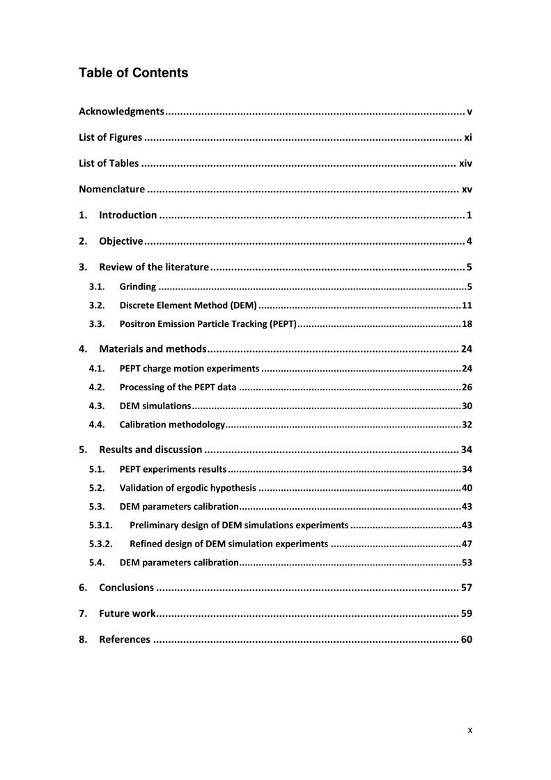
Table of Contents

Acknowledgments .................................................................................................... v

List of Figures .......................................................................................................... xi

List of Tables ......................................................................................................... xiv

Nomenclature ........................................................................................................ xv

1. Introduction ...................................................................................................... 1

2. Objective ........................................................................................................... 4

3. Review of the literature ..................................................................................... 5

3.1. Grinding ............................................................................................................... 5

3.2. Discrete Element Method (DEM) ......................................................................... 11

3.3. Positron Emission Particle Tracking (PEPT) ........................................................... 18

4. Materials and methods .................................................................................... 24

4.1. PEPT charge motion experiments ........................................................................ 24

4.2. Processing of the PEPT data ................................................................................ 26

4.3. DEM simulations ................................................................................................. 30

4.4. Calibration methodology ..................................................................................... 32

5. Results and discussion ..................................................................................... 34

5.1. PEPT experiments results .................................................................................... 34

5.2. Validation of ergodic hypothesis ......................................................................... 40

5.3. DEM parameters calibration ................................................................................ 43

5.3.1. Preliminary design of DEM simulations experiments ........................................ 43

5.3.2. Refined design of DEM simulation experiments ............................................... 47

5.4. DEM parameters calibration ................................................................................ 53

6. Conclusions ..................................................................................................... 57

7. Future work ..................................................................................................... 59

8. References ...................................................................................................... 60

xi

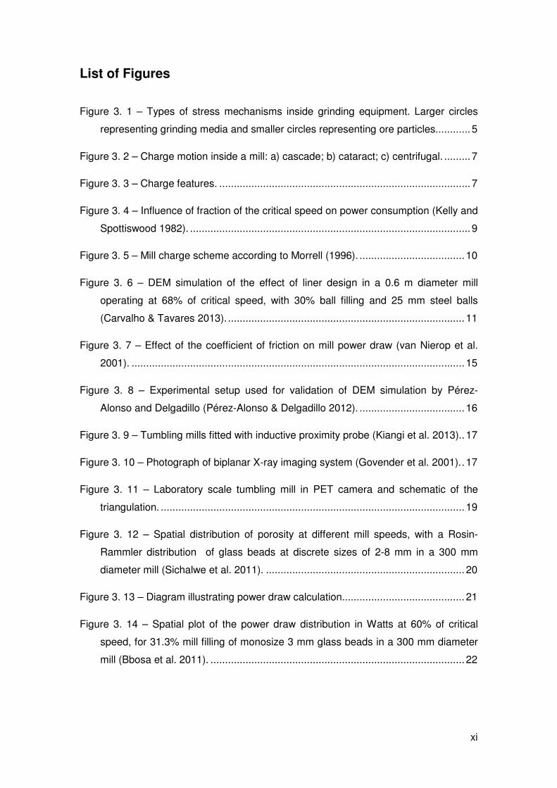
List of Figures

Figure 3. 1 – Types of stress mechanisms inside grinding equipment. Larger circles

representing grinding media and smaller circles representing ore particles. ........... 5

Figure 3. 2 – Charge motion inside a mill: a) cascade; b) cataract; c) centrifugal. ......... 7

Figure 3. 3 – Charge features. ...................................................................................... 7

Figure 3. 4 – Influence of fraction of the critical speed on power consumption (Kelly and

Spottiswood 1982). ................................................................................................ 9

Figure 3. 5 – Mill charge scheme according to Morrell (1996). .................................... 10

Figure 3. 6 – DEM simulation of the effect of liner design in a 0.6 m diameter mill

operating at 68% of critical speed, with 30% ball filling and 25 mm steel balls

(Carvalho & Tavares 2013). ................................................................................. 11

Figure 3. 7 – Effect of the coefficient of friction on mill power draw (van Nierop et al.

2001). .................................................................................................................. 15

Figure 3. 8 – Experimental setup used for validation of DEM simulation by Pérez-

Alonso and Delgadillo (Pérez-Alonso & Delgadillo 2012). .................................... 16

Figure 3. 9 – Tumbling mills fitted with inductive proximity probe (Kiangi et al. 2013). . 17

Figure 3. 10 – Photograph of biplanar X-ray imaging system (Govender et al. 2001). . 17

Figure 3. 11 – Laboratory scale tumbling mill in PET camera and schematic of the

triangulation. ........................................................................................................ 19

Figure 3. 12 – Spatial distribution of porosity at different mill speeds, with a Rosin-

Rammler distribution of glass beads at discrete sizes of 2-8 mm in a 300 mm

diameter mill (Sichalwe et al. 2011). .................................................................... 20

Figure 3. 13 – Diagram illustrating power draw calculation.......................................... 21

Figure 3. 14 – Spatial plot of the power draw distribution in Watts at 60% of critical

speed, for 31.3% mill filling of monosize 3 mm glass beads in a 300 mm diameter

mill (Bbosa et al. 2011). ....................................................................................... 22

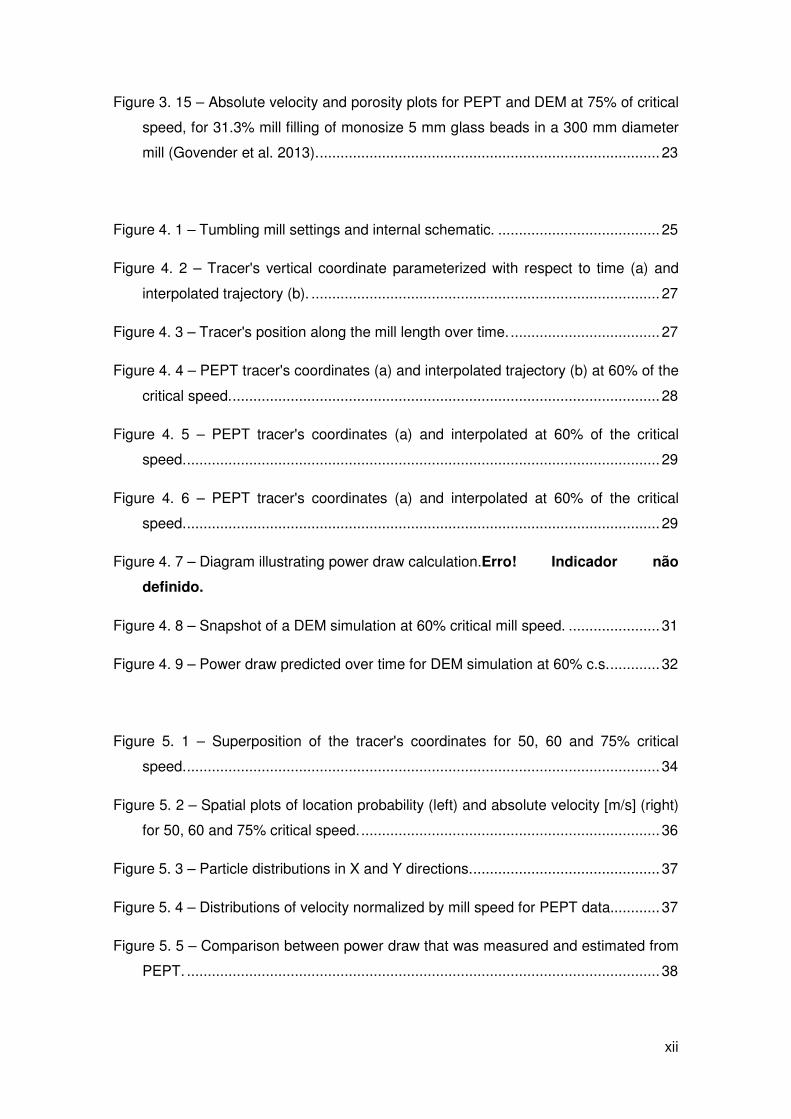
xii

Figure 3. 15 – Absolute velocity and porosity plots for PEPT and DEM at 75% of critical

speed, for 31.3% mill filling of monosize 5 mm glass beads in a 300 mm diameter

mill (Govender et al. 2013). .................................................................................. 23

Figure 4. 1 – Tumbling mill settings and internal schematic. ....................................... 25

Figure 4. 2 – Tracer's vertical coordinate parameterized with respect to time (a) and

interpolated trajectory (b). .................................................................................... 27

Figure 4. 3 – Tracer's position along the mill length over time. .................................... 27

Figure 4. 4 – PEPT tracer's coordinates (a) and interpolated trajectory (b) at 60% of the

critical speed. ....................................................................................................... 28

Figure 4. 5 – PEPT tracer's coordinates (a) and interpolated at 60% of the critical

speed. .................................................................................................................. 29

Figure 4. 6 – PEPT tracer's coordinates (a) and interpolated at 60% of the critical

speed. .................................................................................................................. 29

Figure 4. 7 – Diagram illustrating power draw calculation.Erro! Indicador não

definido.

Figure 4. 8 – Snapshot of a DEM simulation at 60% critical mill speed. ...................... 31

Figure 4. 9 – Power draw predicted over time for DEM simulation at 60% c.s. ............ 32

Figure 5. 1 – Superposition of the tracer's coordinates for 50, 60 and 75% critical

speed. .................................................................................................................. 34

Figure 5. 2 – Spatial plots of location probability (left) and absolute velocity [m/s] (right)

for 50, 60 and 75% critical speed. ........................................................................ 36

Figure 5. 3 – Particle distributions in X and Y directions. ............................................. 37

Figure 5. 4 – Distributions of velocity normalized by mill speed for PEPT data............ 37

Figure 5. 5 – Comparison between power draw that was measured and estimated from

PEPT. .................................................................................................................. 38

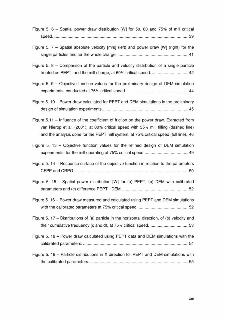
xiii

Figure 5. 6 – Spatial power draw distribution [W] for 50, 60 and 75% of mill critical

speed. .................................................................................................................. 39

Figure 5. 7 – Spatial absolute velocity [m/s] (left) and power draw [W] (right) for the

single particles and for the whole charge. ............................................................ 41

Figure 5. 8 – Comparison of the particle and velocity distribution of a single particle

treated as PEPT, and the mill charge, at 60% critical speed. ............................... 42

Figure 5. 9 – Objective function values for the preliminary design of DEM simulation

experiments, conducted at 75% critical speed. .................................................... 44

Figure 5. 10 – Power draw calculated for PEPT and DEM simulations in the preliminary

design of simulation experiments. ........................................................................ 45

Figure 5.11 – Influence of the coefficient of friction on the power draw. Extracted from

van Nierop et al. (2001), at 80% critical speed with 35% mill filling (dashed line)

and the analysis done for the PEPT mill system, at 75% critical speed (full line). . 46

Figure 5. 13 – Objective function values for the refined design of DEM simulation

experiments, for the mill operating at 75% critical speed. ..................................... 49

Figure 5. 14 – Response surface of the objective function in relation to the parameters

CFPP and CRPG. ................................................................................................ 50

Figure 5. 15 – Spatial power distribution [W] for (a) PEPT, (b) DEM with calibrated

parameters and (c) difference PEPT - DEM. ........................................................ 52

Figure 5. 16 – Power draw measured and calculated using PEPT and DEM simulations

with the calibrated parameters at 75% critical speed. .......................................... 52

Figure 5. 17 – Distributions of (a) particle in the horizontal direction, of (b) velocity and

their cumulative frequency (c and d), at 75% critical speed. ................................. 53

Figure 5. 18 – Power draw calculated using PEPT data and DEM simulations with the

calibrated parameters. ......................................................................................... 54

Figure 5. 19 – Particle distributions in X direction for PEPT and DEM simulations with

the calibrated parameters. ................................................................................... 55

xiv

xv

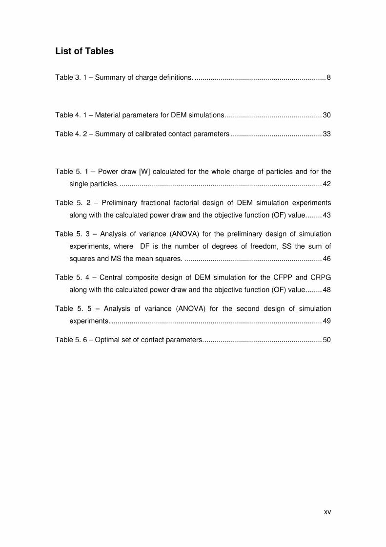
List of Tables

Table 3. 1 – Summary of charge definitions. ................................................................. 8

Table 4. 1 – Material parameters for DEM simulations. ............................................... 30

Table 4. 2 – Summary of calibrated contact parameters ............................................. 33

Table 5. 1 – Power draw [W] calculated for the whole charge of particles and for the

single particles. .................................................................................................... 42

Table 5. 2 – Preliminary fractional factorial design of DEM simulation experiments

along with the calculated power draw and the objective function (OF) value. ....... 43

Table 5. 3 – Analysis of variance (ANOVA) for the preliminary design of simulation

experiments, where DF is the number of degrees of freedom, SS the sum of

squares and MS the mean squares. .................................................................... 46

Table 5. 4 – Central composite design of DEM simulation for the CFPP and CRPG

along with the calculated power draw and the objective function (OF) value. ....... 48

Table 5. 5 – Analysis of variance (ANOVA) for the second design of simulation

experiments. ........................................................................................................ 49

Table 5. 6 – Optimal set of contact parameters. .......................................................... 50

xvi

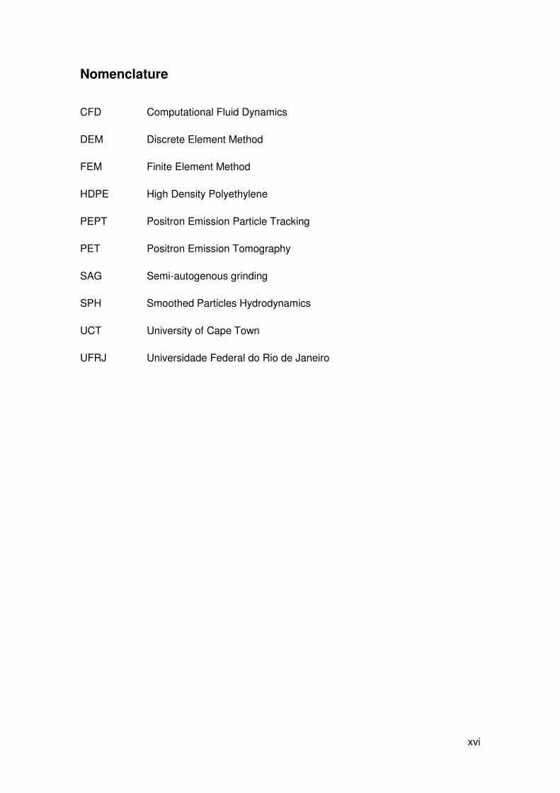
Nomenclature

CFD Computational Fluid Dynamics

DEM Discrete Element Method

FEM Finite Element Method

HDPE High Density Polyethylene

PEPT Positron Emission Particle Tracking

PET Positron Emission Tomography

SAG Semi-autogenous grinding

SPH Smoothed Particles Hydrodynamics

UCT University of Cape Town

UFRJ Universidade Federal do Rio de Janeiro

1

1. Introduction

Tumbling mills are cylindrical shaped equipment with the main purpose of breaking ore

particle to a size where the liberation of the valuable minerals is possible. This class of

equipment is among the most used in the comminution of minerals, presenting great

robustness, and being capable of dealing with large tonnages of material per day and a

wide size range for the feed.

Structurally, this type of mill consists of a horizontal cylindrical shell, equipped with

replaceable wearing liners and a charge of grinding medium. The drum is supported so

as to rotate on its axis, lifting the charge (ore particles and grinding media) and

projecting it. Usually tumbling mills are of three basics types: ball, rod and autogenous.

In the mineral industry, this class of comminution equipment is typically employed in

coarse grinding, in which particles typically between 5 and 250 mm are reduced in size

to between 40 and 300 µm (Wills & Napier-Munn 2006).

Although tumbling mills have been developed to a high degree of mechanical efficiency

and reliability, they are extremely wasteful in terms of energy expended. In a typical

mineral processing plant, around 35% to 50% of the operational costs are related to

comminution (Curry et al. 2014). It is estimated that about 1% of the total electricity

generated in the world is used in crushing and grinding operations (Norgate &

Jahanshahi 2011). For ball mills, values of 15% for energy efficiency in the creation of

new surface area have been estimated (Fuerstenau & Abouzeid 2002).

From the standpoint of the ore, it is estimated that the extraction of metallic minerals

will continue to grow for the next decades. For metals such as copper, iron and

aluminum, processing of the respective ores is expected to double by 2030. However,

the ore grades should continue falling, making its processing and concentration even

more difficult and expensive (Mudd 2010).

Considering all the points presented above, the modeling and complete understanding

of the charge behavior and mechanisms related to particle breakage in tumbling mills

are of extreme importance. Throughout the 20th century, some models relating

operational conditions of mills with particle breakage have been proposed. One of the

first methodologies suggested, and used until today, is the Bond Method, for the

scaling of industrial mills from locked-cycle tests (King 2001). In the 1960s onwards,

more complex models were proposed, considering the population balances and

breakage properties of different size classes.

2

The approaches mentioned above, although useful, present serious limitations since

they do not take into account some construction and operating characteristics of the

mills, such as size and shape of grinding media, liner profile and rotational velocity of

the mill shell. Those limitations come from the fact that tumbling mills are closed and

opaque systems, making the complete quantification of charge distribution and motion

extremely difficult or even impossible. In industrial mills, measurements of feed,

discharge, power draw and mass of charge inside the mills are possible, however,

information about charge motion, size distribution throughout the mill length and

collision energy spectrum between ore and grinding media are still very hard to be

determined. The latter is of extreme importance in the case of Greenfield projects or

those that will process ore with unusual behavior.

In order to overcome this difficulty, Mishra and Rajamani applied in the 1990s the

Discrete Element Method (DEM) for the first time in the simulation of mills. The discrete

element method is a special class of numerical schemes for simulating the behavior of

discrete, interacting bodies. Hence, by its very nature, DEM is highly suitable for the

tumbling mill problem (Mishra & Rajamani 1992). It consists of applying Newton's

second law to particulate bodies in motion and a force displacement model to the

bodies in collision (Mishra & Rajamani 1992). In the last two decades, DEM has been

widely applied in equipment and comminution process modeling, advancing with

increasing computational power.

In order for a DEM simulation to describe the particle movement within a geometry with

fidelity to what is observed in the real environment, it is necessary to use in the method

proper material and contact parameters. Those parameters are not always known a

priori. One way to estimate such parameters is through calibration, by quantitative

comparison of experimental and simulation results. In that sense, it is advantageous to

use laboratory-scale mills, where the measurement of the charge flow might be

possible.

The Positron Emission Particle Tracking (PEPT) presents itself as an ideal technique

for calibrating DEM parameters in some cases. PEPT is a technique for measuring the

flow trajectory of a radioactive particle tracer, in three dimensions, in a granular or fluid

system such as a tumbling mill, at a frequency of up to 250 Hz (Parker et al. 1993). At

the end of the test, it is possible to calculate a statistical distribution of particle density

in each of the tested system regions.

3





4

2. Objective





3. Review of the literature

3.1. Grinding

Since most of the ore mineral

themselves finally associated with

economic value, its liberation is necessary. Such liberation is achieved through

comminution, which consists in the progressive size reduction of particles down to size

ranges required for subsequent concentration. Comminution represents the first stage

in mineral processing after mining and in general is divided into crushing and grinding

stages.

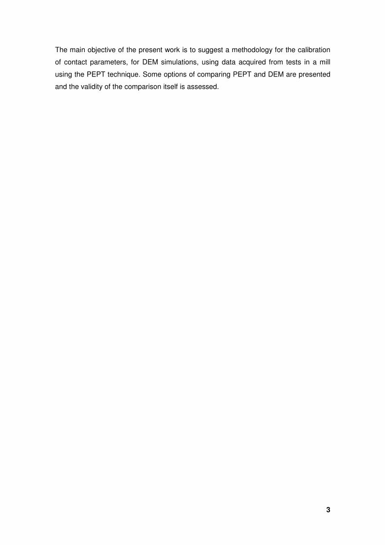
Grinding is usually the last stage in the process of comminution; in this stage particles

are reduced in size by a combination of impact and abrasion, either dry or in

suspension in water. It is performed in rotating cylindrical steel vessels which contain a

charge of loose crushing bodies ̶ the grinding media ̶ which is free to move inside the

mill, thus comminuting the ore particles. Figure

application of stresses involved in grinding equipment. A special kind of grinding

equipment is the tumbling mill. Tumbling mills are typically employed in coarse

grinding, in which particles between 5 and 250 mm are reduced in size to between 40

and 300 µm (Wills & Napier

generally defines the mill. Thus the medium could b

mill is designated as a ball mill

rod mill. When no grinding medium is charged it is known as an

Figure 3. 1 – Types of stress mechanisms inside grinding equipment. Larger circles representing

grinding media and smaller circles representing ore particles.

Review of the literature

minerals, that is, minerals that can extracted profitably, find

themselves finally associated with gangue, which is the rocky material without

s liberation is necessary. Such liberation is achieved through

, which consists in the progressive size reduction of particles down to size


g after mining and in general is divided into crushing and grinding



It is performed in rotating cylindrical steel vessels which contain a


mill, thus comminuting the ore particles. Figure 3.1 illustrates the main modes of

plication of stresses involved in grinding equipment. A special kind of grinding



(Wills & Napier-Munn 2006). The grinding media used in the charge

generally defines the mill. Thus the medium could be steel or cast iron balls, when the

ball mill; or it could be steel rods, where the mill is known as a

. When no grinding medium is charged it is known as an autogenous mill

Types of stress mechanisms inside grinding equipment. Larger circles representing

grinding media and smaller circles representing ore particles.

5

, that is, minerals that can extracted profitably, find

rocky material without

s liberation is necessary. Such liberation is achieved through

, which consists in the progressive size reduction of particles down to size


g after mining and in general is divided into crushing and grinding



It is performed in rotating cylindrical steel vessels which contain a


.1 illustrates the main modes of

plication of stresses involved in grinding equipment. A special kind of grinding



. The grinding media used in the charge

e steel or cast iron balls, when the

; or it could be steel rods, where the mill is known as a

autogenous mill.

Types of stress mechanisms inside grinding equipment. Larger circles representing

6

Grinding is usually performed wet, although in certain applications, such as cement

production, dry grinding is used. When the mill rotates the mixture of grinding media,

ore, and water, known as the mill charge, is intimately mixed, with the medium

comminuting the particles by any of the three kinds of stresses cited above, depending

on the rotational speed of the mill and the shell liner structure.

Several devices are used to promote size reduction of particles inside a conventional

tumbling mill, such as lifters that help to raise the grinding media to greater heights

before they drop and cascade down. Lifters are incorporated in the mill liners, which

are designed with different profiles. They serve the dual purpose of protecting from

wear the steel outer shell of the mill and help lifting the charge. Liner surfaces can be

smooth, ribbed or waved. The rate of wear of liners is roughly proportional to the speed

of rotation of the mill (Gupta & Yan 2006).

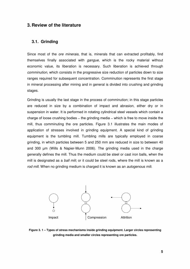
On rotating a mill charged with ore rocks and grinding media, the entire charge rises

against the perimeter of the mill in the direction of the motion. On reaching a certain

height, part of the charge cascades and falls to the bottom of the mill, while the other

part tends to slip down but soon travels again in the direction of motion of the mill.

Figure 3.2 illustrates the charge motion inside a mill. During these processes, the

media drops repeatedly onto the rock, breaking it down to finer sizes. Some size

reduction also takes place due to shear or abrasive forces. As a result of the combined

action of repeated impact and abrasion over time, size reduction takes place and, given

sufficient time, the mineral of interest becomes sufficiently liberated in such a form that

it can be economically recovered.

Depending on the rotational speed and the degree of filling, three types of charge

motion states can be distinguished: cascading, cataracting and centrifuging motion, as

illustrated in Figure 3.2. At relatively low speeds, the medium tends to roll down to the

toe of the mill and predominantly abrasive comminution occurs. This cascading leads

to finer grinding. At higher speeds the medium is projected clear of the charge to

describe a series of parabolas before landing on the toe of the charge. This cataracting

leads to comminution by impact. At the critical speed of the mill the theoretical

trajectory of the medium is such that it would fall outside the shell. In practice,

centrifugal occurs and the medium is carried around in an essentially fixed position

against the shell (Wills & Napier-Munn 2006).

7

Figure 3. 2 – Charge motion inside a mill: a) cascade; b) cataract; c) centrifugal.

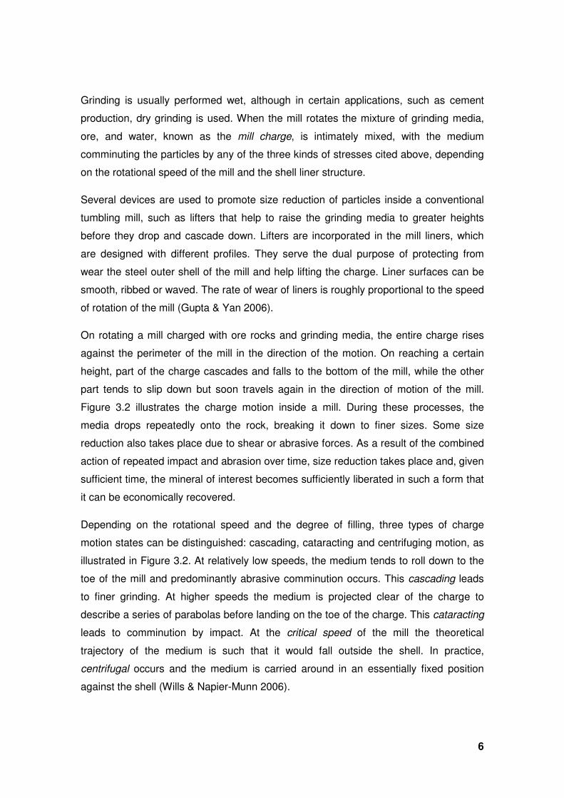
In order to provide a better description of charge motion in relation to mill operation and

construction characteristics, some features of the charge need to be defined. Two such

features are the centre of circulation (CoC) and the equilibrium surface. The CoC is

defined as the point about which all the charge in the mill circulates and the equilibrium

surface as the surface dividing the ascending en masse charge from the descending

charge (Powell & McBride 2004). Figure 3.3 shows a photographic image of a batch

ball mill equipped with a transparent lid and indications of some charge features.

Additional charge features are the departure shoulder ‒ uppermost point t which the

charge departs from the shell of the mill; the head ‒ the highest vertical position that

the charge attains; the bulk toe ‒ turning point of bulk charge against the mill shell; the

impact toe ‒ region, providing the mill speed is sufficiently high, where the cataracting

charge impacts the shell.

Figure 3. 3 – Charge features.

8

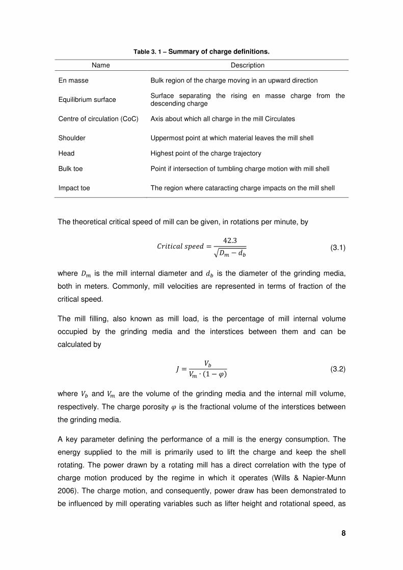
Table 3. 1 – Summary of charge definitions.

Name Description

En masse Bulk region of the charge moving in an upward direction

Equilibrium surface Surface separating the rising en masse charge from the descending charge

Centre of circulation (CoC) Axis about which all charge in the mill Circulates

Shoulder Uppermost point at which material leaves the mill shell

Head Highest point of the charge trajectory

Bulk toe Point if intersection of tumbling charge motion with mill shell

Impact toe The region where cataracting charge impacts on the mill shell

The theoretical critical speed of mill can be given, in rotations per minute, by

�� = 42.3�� − �� (3.1)

where �� is the mill internal diameter and �� is the diameter of the grinding media,

both in meters. Commonly, mill velocities are represented in terms of fraction of the

critical speed.

The mill filling, also known as mill load, is the percentage of mill internal volume

occupied by the grinding media and the interstices between them and can be

calculated by

� = �� ∙ �1 − �� (3.2)

where �� and �� are the volume of the grinding media and the internal mill volume,

respectively. The charge porosity � is the fractional volume of the interstices between

the grinding media.

A key parameter defining the performance of a mill is the energy consumption. The

energy supplied to the mill is primarily used to lift the charge and keep the shell

rotating. The power drawn by a rotating mill has a direct correlation with the type of

charge motion produced by the regime in which it operates (Wills & Napier-Munn

2006). The charge motion, and consequently, power draw has been demonstrated to

be influenced by mill operating variables such as lifter height and rotational speed, as

9

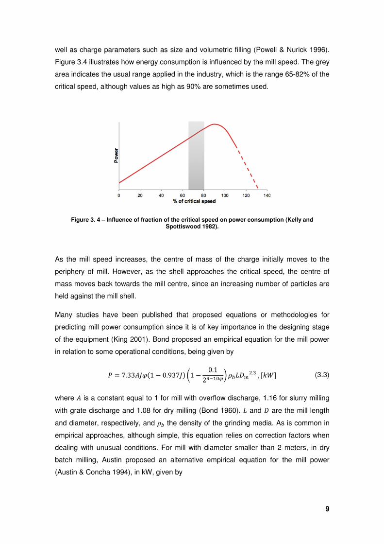
well as charge parameters such as size and volumetric filling (Powell & Nurick 1996).

Figure 3.4 illustrates how energy consumption is influenced by the mill speed. The grey

area indicates the usual range applied in the industry, which is the range 65-82% of the

critical speed, although values as high as 90% are sometimes used.

Figure 3. 4 – Influence of fraction of the critical speed on power consumption (Kelly and Spottiswood 1982).

As the mill speed increases, the centre of mass of the charge initially moves to the

periphery of mill. However, as the shell approaches the critical speed, the centre of

mass moves back towards the mill centre, since an increasing number of particles are

held against the mill shell.

Many studies have been published that proposed equations or methodologies for

predicting mill power consumption since it is of key importance in the designing stage

of the equipment (King 2001). Bond proposed an empirical equation for the mill power

in relation to some operational conditions, being given by

� = 7.33 ��1 − 0.937�� #1 − 0.12$%&'()*�+��,.-, [01] (3.3)

where is a constant equal to 1 for mill with overflow discharge, 1.16 for slurry milling

with grate discharge and 1.08 for dry milling (Bond 1960). + and � are the mill length

and diameter, respectively, and *� the density of the grinding media. As is common in

empirical approaches, although simple, this equation relies on correction factors when

dealing with unusual conditions. For mill with diameter smaller than 2 meters, in dry

batch milling, Austin proposed an alternative empirical equation for the mill power

(Austin & Concha 1994), in kW, given by

10

� = 13.03��'.4 5 �� − 0.1�1 + �7[15.7�� − 0.94�]9 �1 − 0.937��1 + 5.95�4� (3.4)

where 3is the mass of the ball charge, in tons. However useful in various applications,

those equations do not relate the power consumption with charge variables, such as,

grinding media distribution, charge elevation, porosity, etc.

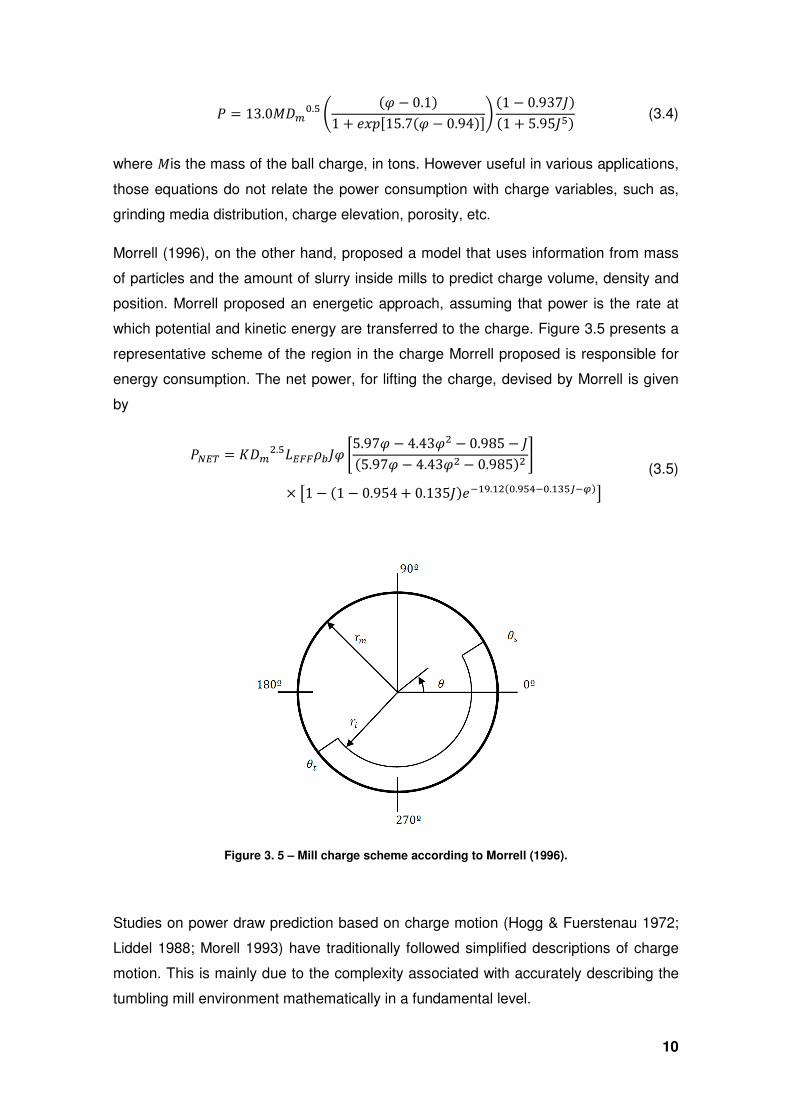
Morrell (1996), on the other hand, proposed a model that uses information from mass

of particles and the amount of slurry inside mills to predict charge volume, density and

position. Morrell proposed an energetic approach, assuming that power is the rate at

which potential and kinetic energy are transferred to the charge. Figure 3.5 presents a

representative scheme of the region in the charge Morrell proposed is responsible for

energy consumption. The net power, for lifting the charge, devised by Morrell is given

by

�:;< = =��,.4+;>>*�� ?5.97� − 4.43�, − 0.985 − ��5.97� − 4.43�, − 0.985�, A

× C1 − �1 − 0.954 + 0.135��%&$.&,�'.$4D%'.&-4E%(�F (3.5)

Figure 3. 5 – Mill charge scheme according to Morrell (1996).

Studies on power draw prediction based on charge motion (Hogg & Fuerstenau 1972;

Liddel 1988; Morell 1993) have traditionally followed simplified descriptions of charge

motion. This is mainly due to the complexity associated with accurately describing the

tumbling mill environment mathematically in a fundamental level.

11

3.2. Discrete Element Method (DEM)

The Discrete Element Method (DEM) however emerged as a means to investigate

particle motion and interaction in enclosed equipment. DEM is a numerical technique

for the simulation of motion and interaction among discrete bodies. Fundamentally,

DEM solves Newton’s equations of motion to resolve particle motion and uses a

contact law to resolve inter-particle contact forces. The contact model describes the

collision mechanics between two or more particles or between particles and the

geometry confining the charge. DEM was firstly developed for studies on soil

mechanics, although for small number of particles (Cundall & Strack 1979). In the

minerals industry, the first application was done a few years later for the simulation of

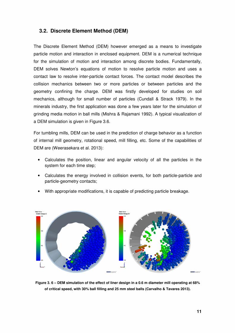
grinding media motion in ball mills (Mishra & Rajamani 1992). A typical visualization of

a DEM simulation is given in Figure 3.6.

For tumbling mills, DEM can be used in the prediction of charge behavior as a function

of internal mill geometry, rotational speed, mill filling, etc. Some of the capabilities of

DEM are (Weerasekara et al. 2013):

• Calculates the position, linear and angular velocity of all the particles in the

system for each time step;

• Calculates the energy involved in collision events, for both particle-particle and

particle-geometry contacts;

• With appropriate modifications, it is capable of predicting particle breakage.

Figure 3. 6 – DEM simulation of the effect of liner design in a 0.6 m diameter mill operating at 68%

of critical speed, with 30% ball filling and 25 mm steel balls (Carvalho & Tavares 2013).

12

In recent years, studies have been carried out on coupling DEM to others computer

simulation techniques, for instance: Gustafsson et al. (2013) applied DEM-FEM

coupling (finite element method) to predict bed breakage of iron ore pellet by

compression; Mayank et al. (2015) used CFD (computational fluid dynamics) coupling

to predict charge and slurry dynamics in tumbling mills; Cleary (2015) simulated wet

grinding in a 36' SAG mill using DEM-SPH (smoothed particles hydrodynamics)

coupling.

The use of coupling techniques allows the application of microscale information on a

macroscale analysis of problem to be solved, providing, in principle, a more realistic

simulation of the charge behavior in a equipment. However, these coupling techniques

require extensive calibration of its models and along with high computational power,

making its application in real size equipment still limited. Additionally validation and

effectiveness of the coupling remains questionable.

Various types of contact relationships are available to describe interactions between

particles. These models include contact between smooth, spherical, non-spherical,

cylindrical, and non-cylindrical elastic particles with friction and surface adhesion

(Mishra 2003). The Hertz-Mindlin contact model (Mindlin 1949) has been used by a

number of researches to conduct DEM simulations of tumbling mills (Tavares &

Carvalho 2010; Khanal & Morrison 2008; Mishra & Cheung 1999). The model is based

on Hertz contact theory and utilizes the linear elasticity model of continuum

environment to calculate the normal force of two perfectly elastic spheres in contact

(Etsion 2010). Since in DEM particles are nondeformable, the key approach of the

method is to consider the solid particles to be able to overlap and collision forces that

result from the relative normal and tangential velocities.

Hertz has showed that two spherical particles of radius �& and �, in contact interact with

applied normal force given by,

GH = IHJ + IHK = −0J LMH& ,N LMH − O0K LMH& DN LPMQH (3.6)

where M is the deformation length of the particles. The stiffness constant 0J is given by,

0J = 43R∗√U (3.7)

and the restitution constant,

13

0K = �HV6XYR∗√UZ& ,N (3.8)

In these equations, �H is the normal restitution coefficient and R∗ depends on the

Young's modulus R,

R∗ = R2�1 − [,� (3.9)

on Poisson's ratio [, and the effective radius U is,

1U = 1�& + 1�, (3.10)

The normal deformation rate, defined by MQH = V\Y] ∙ ^YZ^Y , is function of relative velocity \Y] at the contact point,

\Y] = V\] − \YZ + C_]`�]` ]̂ − _]‖�Y‖^YF (3.11)

where ^Y is the unitary vector that its origin from particle center � respectively in

direction to the contact point with the other particle involved in the contact (particle b) and vice versa. in the case of spheres submitted to an angular load, the tangential

contact force is calculated by Mindlin's model (Mindlin 1949). As in the case of normal

force, the tangential force applied to the particle � is the sum of the repulsion and

damping terms, as

Gc = IcJ + IcK (3.12)

The repulsive force is calculated by,

IcJ = de‖IHJ‖ f1 − 51 − ‖Mc‖g 9- ,N h # Mc‖Mc‖) (3.13)

where de is coefficient of static friction and,

g = de 2 − [�2 − 2[�‖MH‖ (3.14)

is the maximum tangential deformation before slip occurs. In order to satisfy Coulumb

friction law, this force is limited to deIHJ, which results in the relation, 0 ≤ ‖Mc‖ ≤ g.

14

The restitution force is proportional to the tangential deformation rate at the contact

point, MQc , IcK = −�cj

k6XYde‖IHJ‖l1 −‖Mc‖gg m

n& ,N

MQc (3.15)

where �c is the tangential restitution coefficient and the tangential deformation rate is,

MQc = \Y] − V\Y] ∙ ^YZ^Y (2.16)

The acting torque on particle � when it collides against a particle b, may be modeled by

the product of the force acting on the particle and its radius. The resulting torque can

defined as the rolling friction torque, given by,

oY = −dJ‖IHJ‖ _Y‖_Y‖ (3.17)

where dJ is the rolling friction coefficient.

All forces on each of the objects and particles are, then, summed and the following

equations of motion are integrated:

XY �\Y�� =pVGHY + GcYZ + q (3.18)

rY �_Y�� =poY (3.19)

In these equations XY and rY refers to the mass and moment of inertia of particle � and \Y and _Y are their linear and angular velocities.

The key parameters in this model are the coefficient of restitution and the coefficient of

friction. The coefficient of restitution can be defined as the ratio \ \'N , where \ and \' are, respectively, the particle velocity before and after a collision event (Johnson 1985).

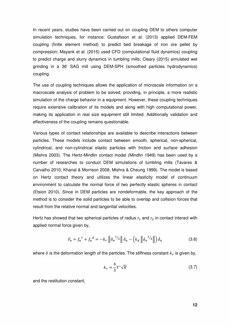
The coefficient of friction is difficult to measure, and it may vary during grinding (Mishra

2003). While Cleary (1998) seemed to suggest that power draw is relatively insensitive

to the choice of value for coefficient of friction, Mishra & Rajamani (1992) and van

Nierop et al. (2001) showed that power draw of ball mills indeed depends on the

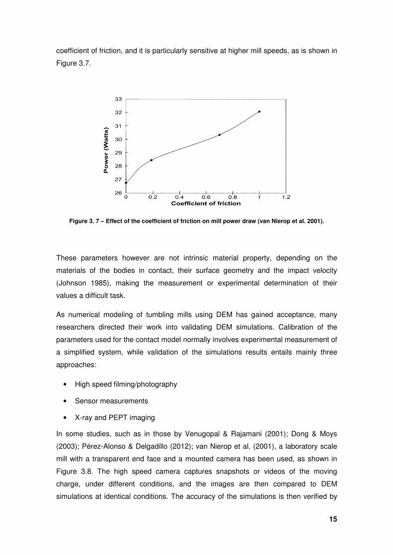
15

coefficient of friction, and it is particularly sensitive at higher mill speeds, as is shown in

Figure 3.7.

Figure 3. 7 – Effect of the coefficient of friction on mill power draw (van Nierop et al. 2001).

These parameters however are not intrinsic material property, depending on the

materials of the bodies in contact, their surface geometry and the impact velocity

(Johnson 1985), making the measurement or experimental determination of their

values a difficult task.

As numerical modeling of tumbling mills using DEM has gained acceptance, many

researchers directed their work into validating DEM simulations. Calibration of the

parameters used for the contact model normally involves experimental measurement of

a simplified system, while validation of the simulations results entails mainly three

approaches:

• High speed filming/photography

• Sensor measurements

• X-ray and PEPT imaging

In some studies, such as in those by Venugopal & Rajamani (2001); Dong & Moys

(2003); Pérez-Alonso & Delgadillo (2012); van Nierop et al. (2001), a laboratory scale

mill with a transparent end face and a mounted camera has been used, as shown in

Figure 3.8. The high speed camera captures snapshots or videos of the moving

charge, under different conditions, and the images are then compared to DEM

simulations at identical conditions. The accuracy of the simulations is then verified by

16

comparing the charge shape and distinguishing features such as toe and shoulder in

experiments and simulations.

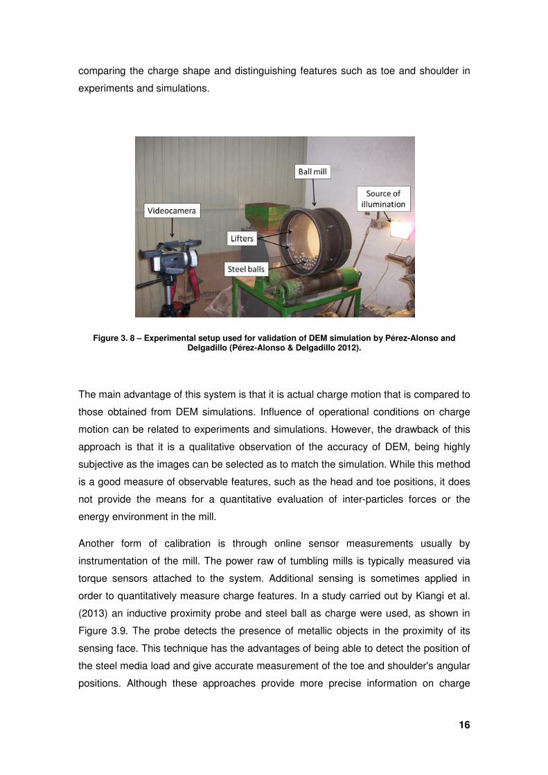
Figure 3. 8 – Experimental setup used for validation of DEM simulation by Pérez-Alonso and Delgadillo (Pérez-Alonso & Delgadillo 2012).

The main advantage of this system is that it is actual charge motion that is compared to

those obtained from DEM simulations. Influence of operational conditions on charge

motion can be related to experiments and simulations. However, the drawback of this

approach is that it is a qualitative observation of the accuracy of DEM, being highly

subjective as the images can be selected as to match the simulation. While this method

is a good measure of observable features, such as the head and toe positions, it does

not provide the means for a quantitative evaluation of inter-particles forces or the

energy environment in the mill.

Another form of calibration is through online sensor measurements usually by

instrumentation of the mill. The power raw of tumbling mills is typically measured via

torque sensors attached to the system. Additional sensing is sometimes applied in

order to quantitatively measure charge features. In a study carried out by Kiangi et al.

(2013) an inductive proximity probe and steel ball as charge were used, as shown in

Figure 3.9. The probe detects the presence of metallic objects in the proximity of its

sensing face. This technique has the advantages of being able to detect the position of

the steel media load and give accurate measurement of the toe and shoulder's angular

positions. Although these approaches provide more precise information on charge

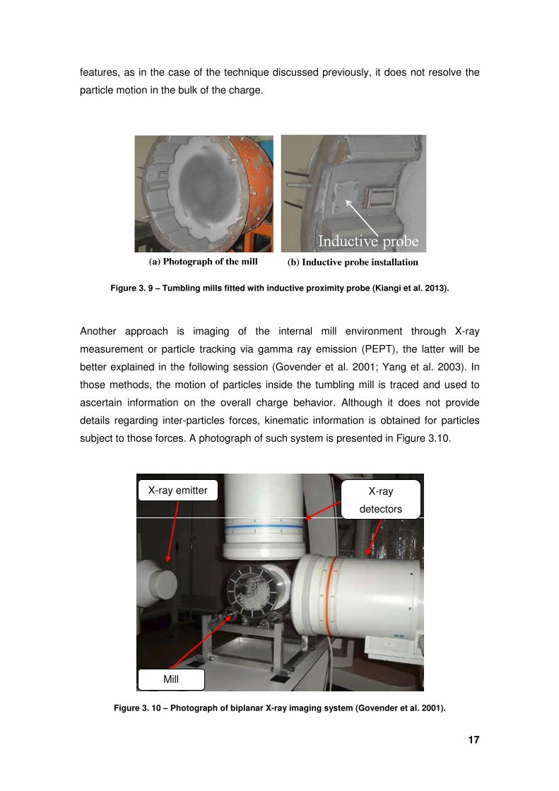
17

features, as in the case of the technique discussed previously, it does not resolve the

particle motion in the bulk of the charge.

Figure 3. 9 – Tumbling mills fitted with inductive proximity probe (Kiangi et al. 2013).

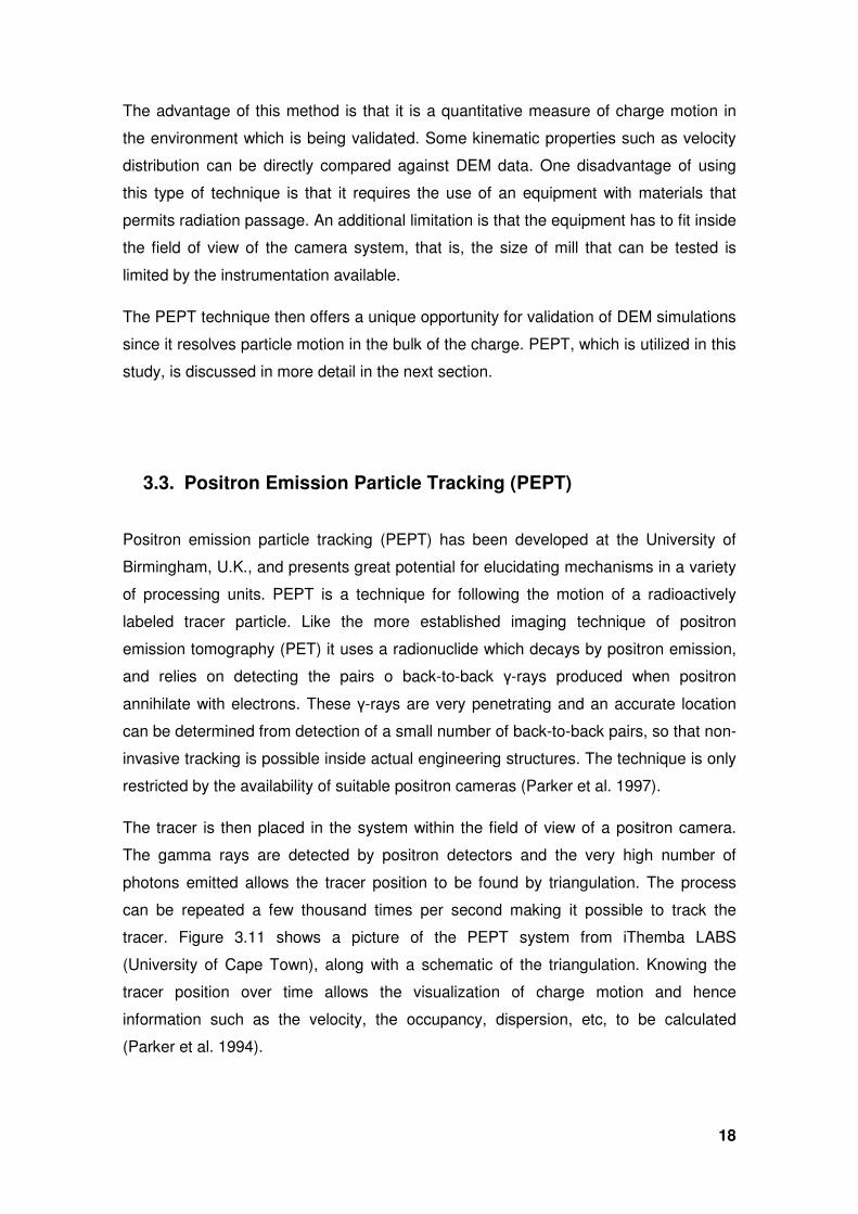
Another approach is imaging of the internal mill environment through X-ray

measurement or particle tracking via gamma ray emission (PEPT), the latter will be

better explained in the following session (Govender et al. 2001; Yang et al. 2003). In

those methods, the motion of particles inside the tumbling mill is traced and used to

ascertain information on the overall charge behavior. Although it does not provide

details regarding inter-particles forces, kinematic information is obtained for particles

subject to those forces. A photograph of such system is presented in Figure 3.10.

Figure 3. 10 – Photograph of biplanar X-ray imaging system (Govender et al. 2001).

Mill

X-ray emitter X-ray

detectors

18

The advantage of this method is that it is a quantitative measure of charge motion in

the environment which is being validated. Some kinematic properties such as velocity

distribution can be directly compared against DEM data. One disadvantage of using

this type of technique is that it requires the use of an equipment with materials that

permits radiation passage. An additional limitation is that the equipment has to fit inside

the field of view of the camera system, that is, the size of mill that can be tested is

limited by the instrumentation available.

The PEPT technique then offers a unique opportunity for validation of DEM simulations

since it resolves particle motion in the bulk of the charge. PEPT, which is utilized in this

study, is discussed in more detail in the next section.

3.3. Positron Emission Particle Tracking (PEPT)

Positron emission particle tracking (PEPT) has been developed at the University of

Birmingham, U.K., and presents great potential for elucidating mechanisms in a variety

of processing units. PEPT is a technique for following the motion of a radioactively

labeled tracer particle. Like the more established imaging technique of positron

emission tomography (PET) it uses a radionuclide which decays by positron emission,

and relies on detecting the pairs o back-to-back γ-rays produced when positron

annihilate with electrons. These γ-rays are very penetrating and an accurate location

can be determined from detection of a small number of back-to-back pairs, so that non-

invasive tracking is possible inside actual engineering structures. The technique is only

restricted by the availability of suitable positron cameras (Parker et al. 1997).

The tracer is then placed in the system within the field of view of a positron camera.

The gamma rays are detected by positron detectors and the very high number of

photons emitted allows the tracer position to be found by triangulation. The process

can be repeated a few thousand times per second making it possible to track the

tracer. Figure 3.11 shows a picture of the PEPT system from iThemba LABS

(University of Cape Town), along with a schematic of the triangulation. Knowing the

tracer position over time allows the visualization of charge motion and hence

information such as the velocity, the occupancy, dispersion, etc, to be calculated

(Parker et al. 1994).

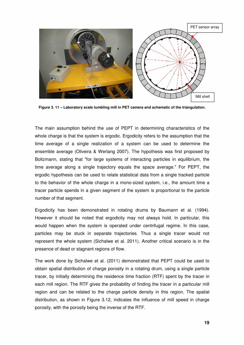
19

Figure 3. 11 – Laboratory scale tumbling mill in PET camera and schematic of the triangulation.

The main assumption behind the use of PEPT in determining characteristics of the

whole charge is that the system is ergodic. Ergodicity refers to the assumption that the

time average of a single realization of a system can be used to determine the

ensemble average (Oliveira & Werlang 2007). The hypothesis was first proposed by

Boltzmann, stating that "for large systems of interacting particles in equilibrium, the

time average along a single trajectory equals the space average." For PEPT, the

ergodic hypothesis can be used to relate statistical data from a single tracked particle

to the behavior of the whole charge in a mono-sized system, i.e., the amount time a

tracer particle spends in a given segment of the system is proportional to the particle

number of that segment.

Ergodicity has been demonstrated in rotating drums by Baumann et al. (1994).

However it should be noted that ergodicity may not always hold. In particular, this

would happen when the system is operated under centrifugal regime. In this case,

particles may be stuck in separate trajectories. Thus a single tracer would not

represent the whole system (Sichalwe et al. 2011). Another critical scenario is in the

presence of dead or stagnant regions of flow.

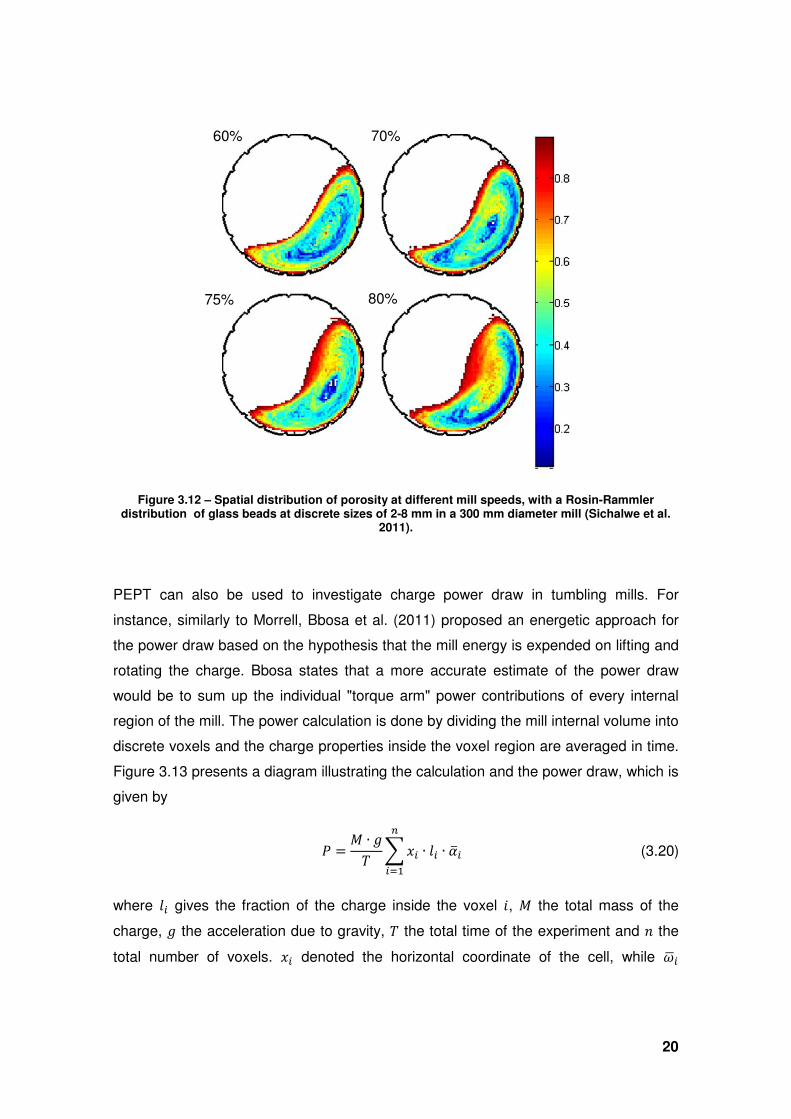
The work done by Sichalwe et al. (2011) demonstrated that PEPT could be used to

obtain spatial distribution of charge porosity in a rotating drum, using a single particle

tracer, by initially determining the residence time fraction (RTF) spent by the tracer in

each mill region. The RTF gives the probability of finding the tracer in a particular mill

region and can be related to the charge particle density in this region. The spatial

distribution, as shown in Figure 3.12, indicates the influence of mill speed in charge

porosity, with the porosity being the inverse of the RTF.

PET sensor array

Mill shell

20

Figure 3.12 – Spatial distribution of porosity at different mill speeds, with a Rosin-Rammler distribution of glass beads at discrete sizes of 2-8 mm in a 300 mm diameter mill (Sichalwe et al.

2011).

PEPT can also be used to investigate charge power draw in tumbling mills. For

instance, similarly to Morrell, Bbosa et al. (2011) proposed an energetic approach for

the power draw based on the hypothesis that the mill energy is expended on lifting and

rotating the charge. Bbosa states that a more accurate estimate of the power draw

would be to sum up the individual "torque arm" power contributions of every internal

region of the mill. The power calculation is done by dividing the mill internal volume into

discrete voxels and the charge properties inside the voxel region are averaged in time.

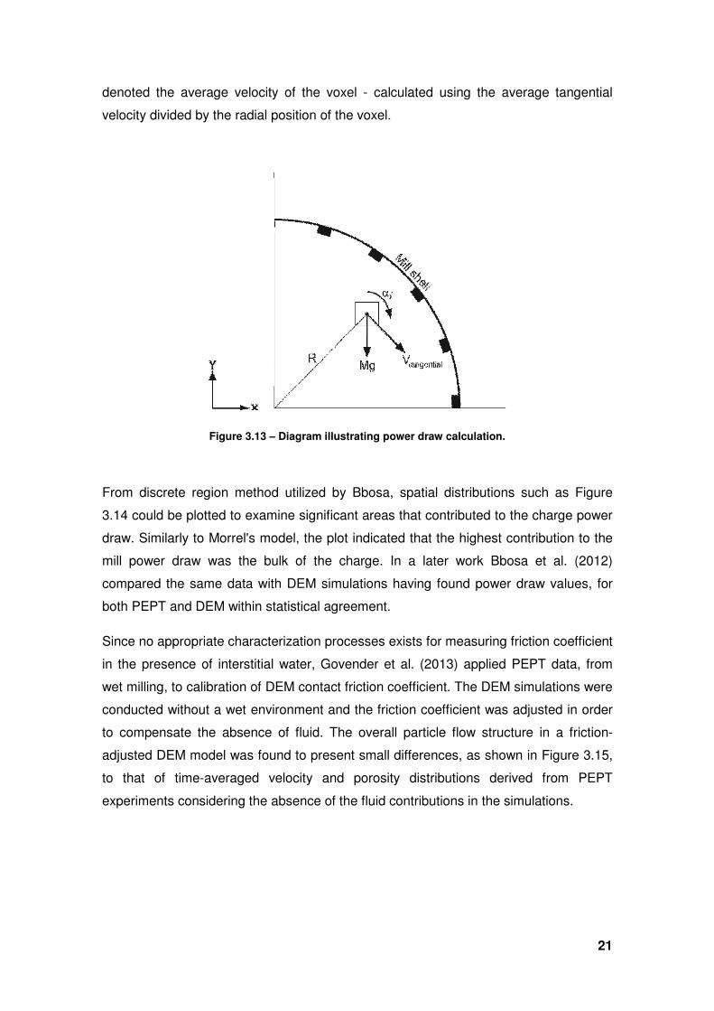
Figure 3.13 presents a diagram illustrating the calculation and the power draw, which is

given by

� = 3 ∙ qo p7Y ∙ �Y ∙ stYHYu& (3.20)

where �Y gives the fraction of the charge inside the voxel �, 3 the total mass of the

charge, q the acceleration due to gravity, o the total time of the experiment and ^ the

total number of voxels. 7Y denoted the horizontal coordinate of the cell, while _vY

60% 70%

75% 80%

21

denoted the average velocity of the voxel - calculated using the average tangential

velocity divided by the radial position of the voxel.

Figure 3.13 – Diagram illustrating power draw calculation.

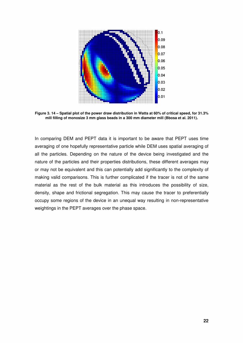
From discrete region method utilized by Bbosa, spatial distributions such as Figure

3.14 could be plotted to examine significant areas that contributed to the charge power

draw. Similarly to Morrel's model, the plot indicated that the highest contribution to the

mill power draw was the bulk of the charge. In a later work Bbosa et al. (2012)

compared the same data with DEM simulations having found power draw values, for

both PEPT and DEM within statistical agreement.

Since no appropriate characterization processes exists for measuring friction coefficient

in the presence of interstitial water, Govender et al. (2013) applied PEPT data, from

wet milling, to calibration of DEM contact friction coefficient. The DEM simulations were

conducted without a wet environment and the friction coefficient was adjusted in order

to compensate the absence of fluid. The overall particle flow structure in a friction-

adjusted DEM model was found to present small differences, as shown in Figure 3.15,

to that of time-averaged velocity and porosity distributions derived from PEPT

experiments considering the absence of the fluid contributions in the simulations.

22

Figure 3. 14 – Spatial plot of the power draw distribution in Watts at 60% of critical speed, for 31.3%

mill filling of monosize 3 mm glass beads in a 300 mm diameter mill (Bbosa et al. 2011).

In comparing DEM and PEPT data it is important to be aware that PEPT uses time

averaging of one hopefully representative particle while DEM uses spatial averaging of

all the particles. Depending on the nature of the device being investigated and the

nature of the particles and their properties distributions, these different averages may

or may not be equivalent and this can potentially add significantly to the complexity of

making valid comparisons. This is further complicated if the tracer is not of the same

material as the rest of the bulk material as this introduces the possibility of size,

density, shape and frictional segregation. This may cause the tracer to preferentially

occupy some regions of the device in an unequal way resulting in non-representative

weightings in the PEPT averages over the phase space.

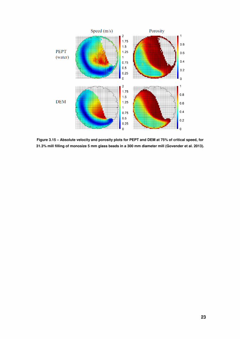
Figure 3.15 – Absolute velocity and porosity plots for PEPT and DEM at 75% of critical speed, for

31.3% mill filling of monosize 5 mm glass beads in a 300 mm diameter mill

Absolute velocity and porosity plots for PEPT and DEM at 75% of critical speed, for

31.3% mill filling of monosize 5 mm glass beads in a 300 mm diameter mill (Govender et al. 2013)

23

Absolute velocity and porosity plots for PEPT and DEM at 75% of critical speed, for

(Govender et al. 2013).

24

4. Materials and methods

4.1. PEPT charge motion experiments

For this study three dry tests with only grinding media as charge were performed,

varying mill speed. Single particle tracking experiments using PEPT were conducted

using the ADAC Forte parallel plate camera at the Positron Imaging Centre, installed at

the University of Birmingham, consisting of two heads, each containing a single crystal

of NaI(Tl) scintillator, 500 x 400 mm², optically coupled to an array of 55 photomultiplier

tubes (Parker et al. 2002). Tracking was possible over the volume between the two

front faces of the detectors, giving a maximum field of view of 800 x 500 x 400 mm³.

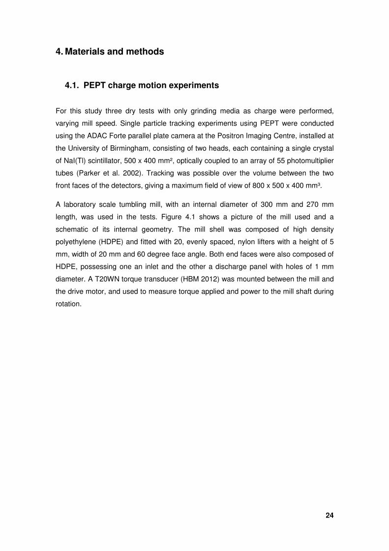
A laboratory scale tumbling mill, with an internal diameter of 300 mm and 270 mm

length, was used in the tests. Figure 4.1 shows a picture of the mill used and a

schematic of its internal geometry. The mill shell was composed of high density

polyethylene (HDPE) and fitted with 20, evenly spaced, nylon lifters with a height of 5

mm, width of 20 mm and 60 degree face angle. Both end faces were also composed of

HDPE, possessing one an inlet and the other a discharge panel with holes of 1 mm

diameter. A T20WN torque transducer (HBM 2012) was mounted between the mill and

the drive motor, and used to measure torque applied and power to the mill shaft during

rotation.

25

Figure 4. 1 – Tumbling mill settings and internal schematic.

Five-millimeter spherical glass beads were used as charge, comprising a constant

volumetric mill filling of 31.3%. The total mass of the charge inside the mill was

calculated using the equation 4.1,

3 = �1 − �� ∙ � ∙ �w ∙ *x (4.1)

being �w the mill internal volume, � the mill filling, and *x and � are the charge density

and porosity respectively. The glass bead density was 2500 kg/m³. The porosity

represents the fraction of the volume occupied by the charge, in the mill, which is

empty space. There are various protocols to determine the random close packing of

spheres with the same diameter, and the resultant porosity is dependent on the

protocol employed (Torquato et al. 2000). The densest possible in a three dimension

packing is the close-packed hexagonal structure, which has ϕ ≈ 0.26. However, in a

vibrating or dynamic system, such an orderly configuration is not realistic and values

around ϕ = 0.40 are usually assumed (Jaeger & Nagel 1992). In a work done by Bbosa

(Bbosa et al. 2011) using the same batch of PEPT data, a porosity of 0.37 was

assumed with good agreement with the experimental results, thus the same value was

used in the present work.

26

A single 5 mm glass bead was subjected to direct activation using a 33MeV ³He beam

for use as radioactive tracer particle. Following the methodology described by Parker et

al. (1997), the bead was labeled with 18F, which has a half-life of approximately 110

min. Before and after each test, the radioactivity of the tracer particle was measured

using a Geiger counter. This was done to ensure that the level of radioactivity on the

tracer was at least 300 µCi, which was the recommended minimum for the parallel

plate PEPT camera (Parker & Fan 2008). In each test, the activated glass bead was

added to the charge in the mill and its motion was tracked for an hour.

All the experimental procedures done for this work were performed by Centre for

Mineral Research at the University of Cape Town (CMR-UCT) and shared with the

Laboratório de Tecnologia Mineral - COPPE/UFRJ.

4.2. Processing of the PEPT data

The output of the triangulation algorithm, used to extract the PEPT data, was a text file

which contained the Cartesian coordinates of the tracer for the duration of the

experiment, after steady state has been reached. The 3D data points, in millimeters,

and with time t in milliseconds were then imported into a MATLAB® routine for the

PEPT data analysis.

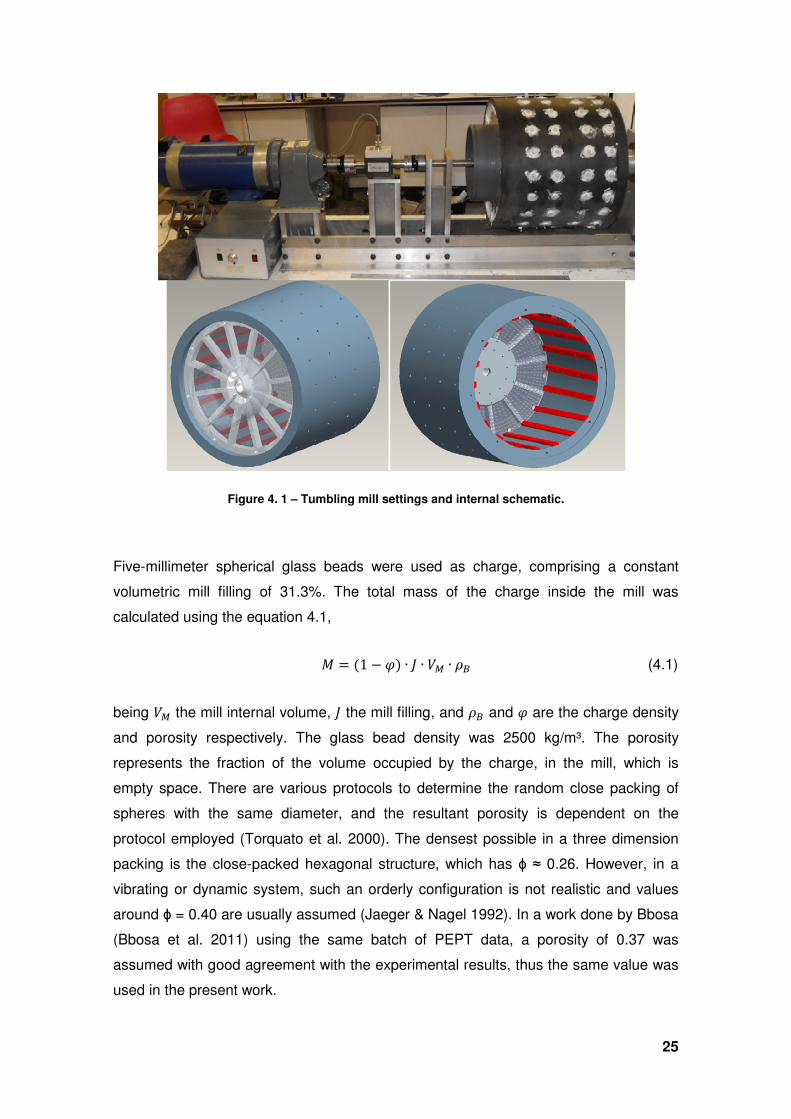
For convenience, the origin is specified as the mill center, with coordinates x

(horizontal) and y (vertical) in the transverse plane, while z along the axial mill length

with zero at the one of the end faces. The triangulated coordinates, positions x, y and

z, could be parameterized with respect to time t, as shown by the points in Figure 4.2.

From the parameterized coordinate a cubic spline interpolation was done, with even

time intervals, thus a more detailed trajectory could be approximated (line in Figure

4.2).

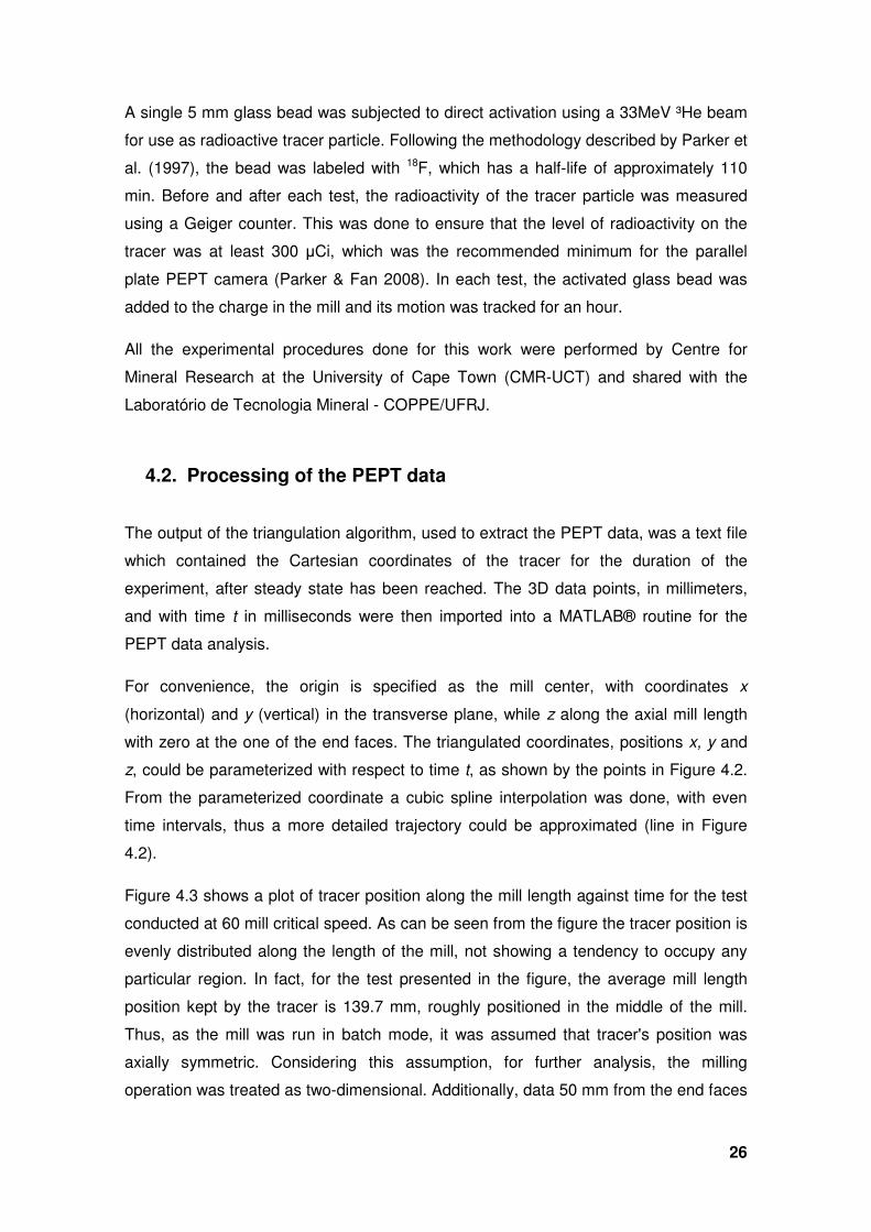
Figure 4.3 shows a plot of tracer position along the mill length against time for the test

conducted at 60 mill critical speed. As can be seen from the figure the tracer position is

evenly distributed along the length of the mill, not showing a tendency to occupy any

particular region. In fact, for the test presented in the figure, the average mill length

position kept by the tracer is 139.7 mm, roughly positioned in the middle of the mill.

Thus, as the mill was run in batch mode, it was assumed that tracer's position was

axially symmetric. Considering this assumption, for further analysis, the milling

operation was treated as two-dimensional. Additionally, data 50 mm from the end faces

27

were removed from the calculations in order to avoid any border effect. Thus, the

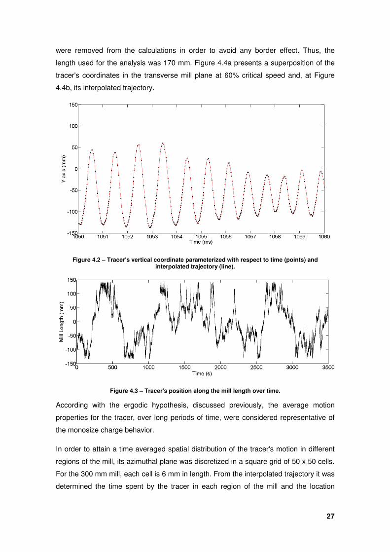
length used for the analysis was 170 mm. Figure 4.4a presents a superposition of the

tracer's coordinates in the transverse mill plane at 60% critical speed and, at Figure

4.4b, its interpolated trajectory.

Figure 4.2 – Tracer's vertical coordinate parameterized with respect to time (points) and interpolated trajectory (line).

Figure 4.3 – Tracer's position along the mill length over time.

According with the ergodic hypothesis, discussed previously, the average motion

properties for the tracer, over long periods of time, were considered representative of

the monosize charge behavior.

In order to attain a time averaged spatial distribution of the tracer's motion in different

regions of the mill, its azimuthal plane was discretized in a square grid of 50 x 50 cells.

For the 300 mm mill, each cell is 6 mm in length. From the interpolated trajectory it was

determined the time spent by the tracer in each region of the mill and the location

28

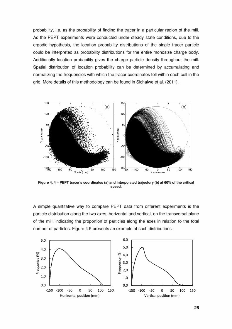
probability, i.e. as the probability of finding the tracer in a particular region of the mill.

As the PEPT experiments were conducted under steady state conditions, due to the

ergodic hypothesis, the location probability distributions of the single tracer particle

could be interpreted as probability distributions for the entire monosize charge body.

Additionally location probability gives the charge particle density throughout the mill.

Spatial distribution of location probability can be determined by accumulating and

normalizing the frequencies with which the tracer coordinates fell within each cell in the

grid. More details of this methodology can be found in Sichalwe et al. (2011).

Figure 4. 4 – PEPT tracer's coordinates (a) and interpolated trajectory (b) at 60% of the critical speed.

A simple quantitative way to compare PEPT data from different experiments is the

particle distribution along the two axes, horizontal and vertical, on the transversal plane

of the mill, indicating the proportion of particles along the axes in relation to the total

number of particles. Figure 4.5 presents an example of such distributions.

0,0

1,0

2,0

3,0

4,0

5,0

-150 -100 -50 0 50 100 150

Fre

qu

en

cy (

%)

Horizontal position (mm)

0,0

1,0

2,0

3,0

4,0

5,0

6,0

-150 -100 -50 0 50 100 150

Fre

qu

en

cy (

%)

Vertical position (mm)

(a) (b)

29

Figure 4. 5 – PEPT tracer's coordinates (a) and interpolated at 60% of the critical speed.

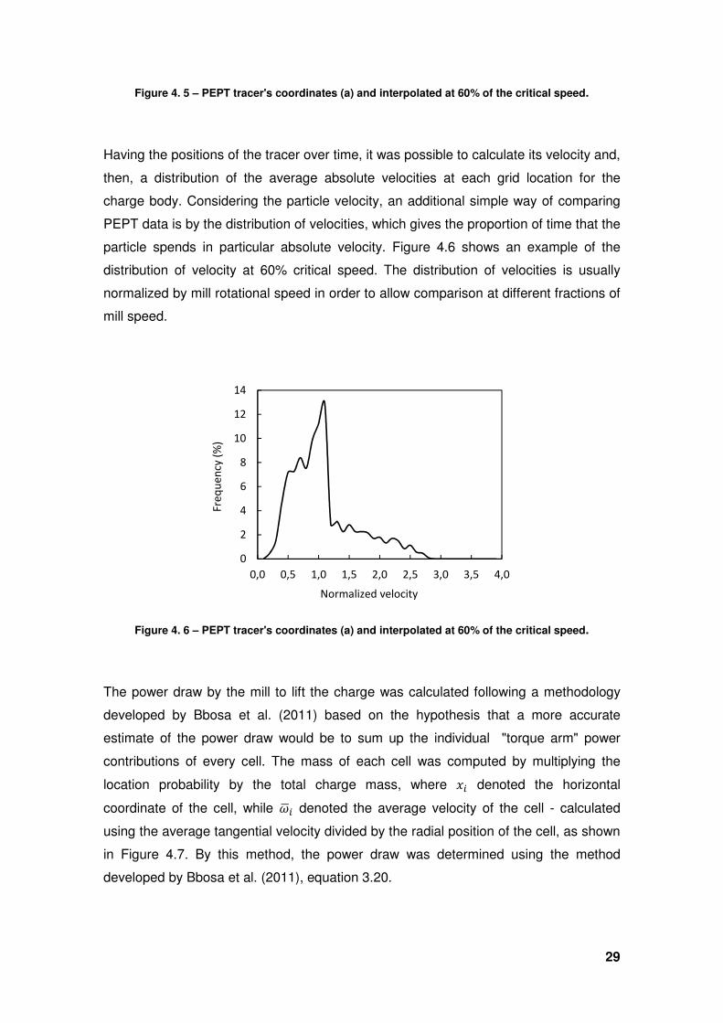
Having the positions of the tracer over time, it was possible to calculate its velocity and,

then, a distribution of the average absolute velocities at each grid location for the

charge body. Considering the particle velocity, an additional simple way of comparing

PEPT data is by the distribution of velocities, which gives the proportion of time that the

particle spends in particular absolute velocity. Figure 4.6 shows an example of the

distribution of velocity at 60% critical speed. The distribution of velocities is usually

normalized by mill rotational speed in order to allow comparison at different fractions of

mill speed.

Figure 4. 6 – PEPT tracer's coordinates (a) and interpolated at 60% of the critical speed.

The power draw by the mill to lift the charge was calculated following a methodology

developed by Bbosa et al. (2011) based on the hypothesis that a more accurate

estimate of the power draw would be to sum up the individual "torque arm" power

contributions of every cell. The mass of each cell was computed by multiplying the

location probability by the total charge mass, where 7Y denoted the horizontal

coordinate of the cell, while _vY denoted the average velocity of the cell - calculated

using the average tangential velocity divided by the radial position of the cell, as shown

in Figure 4.7. By this method, the power draw was determined using the method

developed by Bbosa et al. (2011), equation 3.20.

0

2

4

6

8

10

12

14

0,0 0,5 1,0 1,5 2,0 2,5 3,0 3,5 4,0

Fre

qu

en

cy (

%)

Normalized velocity

30

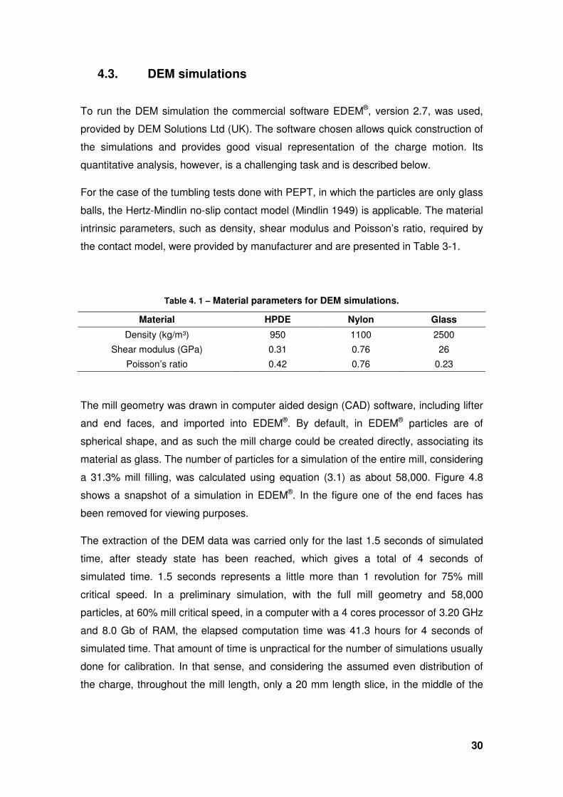
4.3. DEM simulations

To run the DEM simulation the commercial software EDEM®, version 2.7, was used,

provided by DEM Solutions Ltd (UK). The software chosen allows quick construction of

the simulations and provides good visual representation of the charge motion. Its

quantitative analysis, however, is a challenging task and is described below.

For the case of the tumbling tests done with PEPT, in which the particles are only glass

balls, the Hertz-Mindlin no-slip contact model (Mindlin 1949) is applicable. The material

intrinsic parameters, such as density, shear modulus and Poisson’s ratio, required by

the contact model, were provided by manufacturer and are presented in Table 3-1.

Table 4. 1 – Material parameters for DEM simulations.

Material HPDE Nylon Glass

Density (kg/m³) 950 1100 2500

Shear modulus (GPa) 0.31 0.76 26

Poisson’s ratio 0.42 0.76 0.23

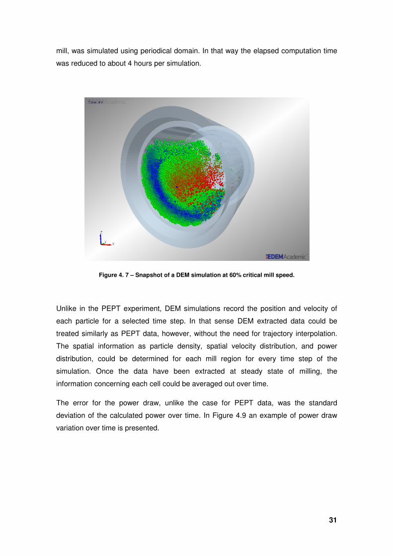
The mill geometry was drawn in computer aided design (CAD) software, including lifter

and end faces, and imported into EDEM®. By default, in EDEM® particles are of

spherical shape, and as such the mill charge could be created directly, associating its

material as glass. The number of particles for a simulation of the entire mill, considering

a 31.3% mill filling, was calculated using equation (3.1) as about 58,000. Figure 4.8

shows a snapshot of a simulation in EDEM®. In the figure one of the end faces has

been removed for viewing purposes.

The extraction of the DEM data was carried only for the last 1.5 seconds of simulated

time, after steady state has been reached, which gives a total of 4 seconds of

simulated time. 1.5 seconds represents a little more than 1 revolution for 75% mill

critical speed. In a preliminary simulation, with the full mill geometry and 58,000

particles, at 60% mill critical speed, in a computer with a 4 cores processor of 3.20 GHz

and 8.0 Gb of RAM, the elapsed computation time was 41.3 hours for 4 seconds of

simulated time. That amount of time is unpractical for the number of simulations usually

done for calibration. In that sense, and considering the assumed even distribution of

the charge, throughout the mill length, only a 20 mm length slice, in the middle of the

31

mill, was simulated using periodical domain. In that way the elapsed computation time

was reduced to about 4 hours per simulation.

Figure 4. 7 – Snapshot of a DEM simulation at 60% critical mill speed.

Unlike in the PEPT experiment, DEM simulations record the position and velocity of

each particle for a selected time step. In that sense DEM extracted data could be

treated similarly as PEPT data, however, without the need for trajectory interpolation.

The spatial information as particle density, spatial velocity distribution, and power

distribution, could be determined for each mill region for every time step of the

simulation. Once the data have been extracted at steady state of milling, the

information concerning each cell could be averaged out over time.

The error for the power draw, unlike the case for PEPT data, was the standard

deviation of the calculated power over time. In Figure 4.9 an example of power draw

variation over time is presented.

32

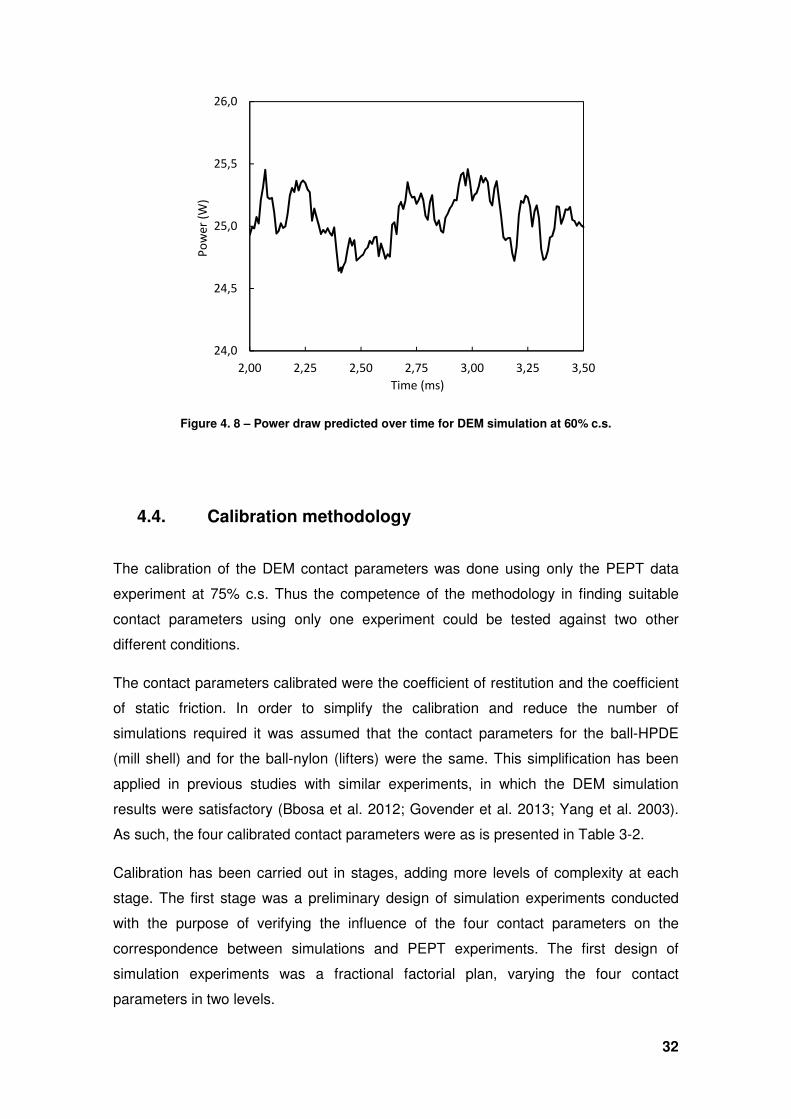
Figure 4. 8 – Power draw predicted over time for DEM simulation at 60% c.s.

4.4. Calibration methodology

The calibration of the DEM contact parameters was done using only the PEPT data

experiment at 75% c.s. Thus the competence of the methodology in finding suitable

contact parameters using only one experiment could be tested against two other

different conditions.

The contact parameters calibrated were the coefficient of restitution and the coefficient

of static friction. In order to simplify the calibration and reduce the number of

simulations required it was assumed that the contact parameters for the ball-HPDE

(mill shell) and for the ball-nylon (lifters) were the same. This simplification has been

applied in previous studies with similar experiments, in which the DEM simulation

results were satisfactory (Bbosa et al. 2012; Govender et al. 2013; Yang et al. 2003).

As such, the four calibrated contact parameters were as is presented in Table 3-2.

Calibration has been carried out in stages, adding more levels of complexity at each

stage. The first stage was a preliminary design of simulation experiments conducted

with the purpose of verifying the influence of the four contact parameters on the

correspondence between simulations and PEPT experiments. The first design of

simulation experiments was a fractional factorial plan, varying the four contact

parameters in two levels.

24,0

24,5

25,0

25,5

26,0

2,00 2,25 2,50 2,75 3,00 3,25 3,50

Po

we

r (W

)

Time (ms)

33

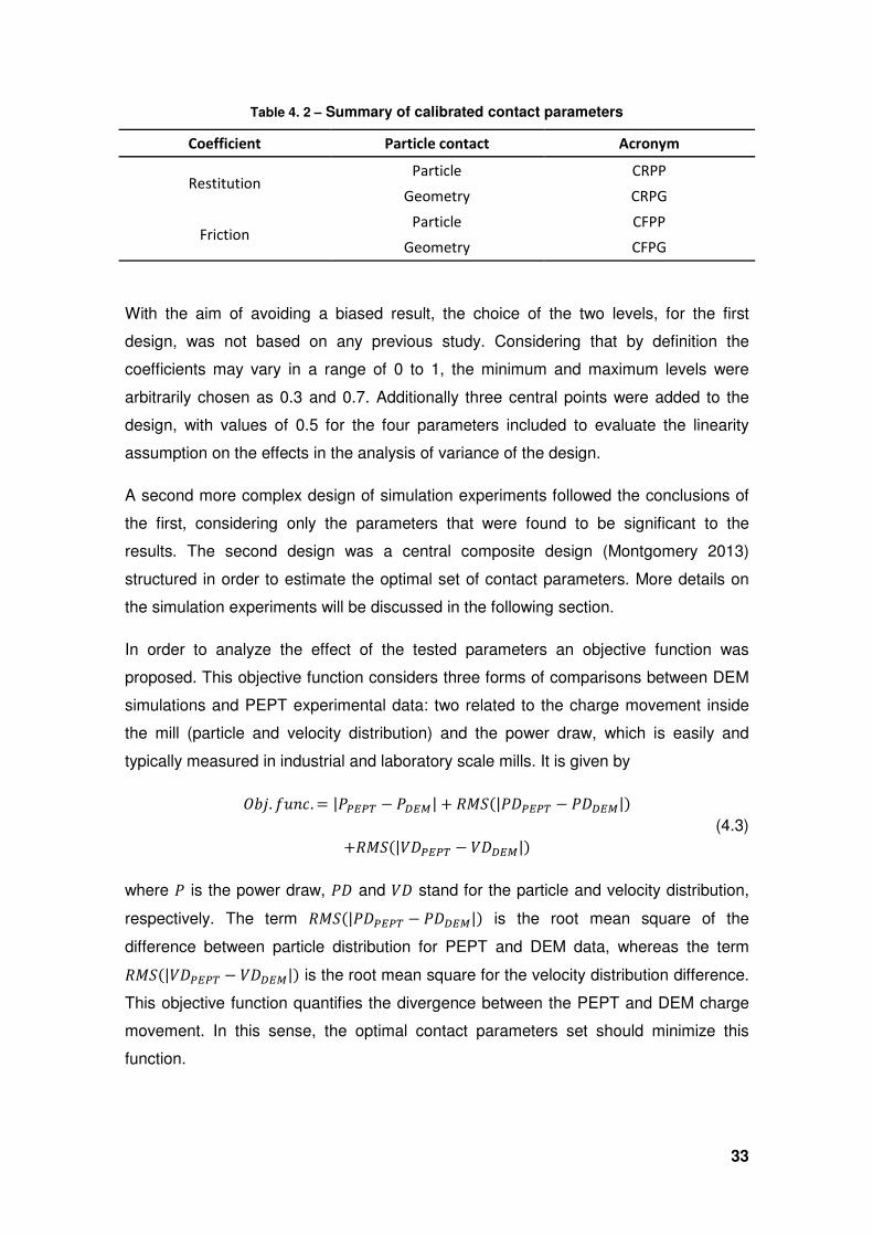
Table 4. 2 – Summary of calibrated contact parameters

Coefficient Particle contact Acronym

Restitution Particle CRPP

Geometry CRPG

Friction Particle CFPP

Geometry CFPG

With the aim of avoiding a biased result, the choice of the two levels, for the first

design, was not based on any previous study. Considering that by definition the

coefficients may vary in a range of 0 to 1, the minimum and maximum levels were

arbitrarily chosen as 0.3 and 0.7. Additionally three central points were added to the

design, with values of 0.5 for the four parameters included to evaluate the linearity

assumption on the effects in the analysis of variance of the design.

A second more complex design of simulation experiments followed the conclusions of

the first, considering only the parameters that were found to be significant to the

results. The second design was a central composite design (Montgomery 2013)

structured in order to estimate the optimal set of contact parameters. More details on

the simulation experiments will be discussed in the following section.

In order to analyze the effect of the tested parameters an objective function was

proposed. This objective function considers three forms of comparisons between DEM

simulations and PEPT experimental data: two related to the charge movement inside

the mill (particle and velocity distribution) and the power draw, which is easily and

typically measured in industrial and laboratory scale mills. It is given by

yzb. I{^�.= |�};}< − �~;w| + U3��|��};}< − ��~;w|� +U3��|��};}< − ��~;w|� (4.3)

where � is the power draw, �� and �� stand for the particle and velocity distribution,

respectively. The term U3��|��};}< − ��~;w|� is the root mean square of the

difference between particle distribution for PEPT and DEM data, whereas the term U3��|��};}< − ��~;w|� is the root mean square for the velocity distribution difference.

This objective function quantifies the divergence between the PEPT and DEM charge

movement. In this sense, the optimal contact parameters set should minimize this

function.

5. Results and discussion

5.1. PEPT experiments results

In this section the results and analysis of the PEPT experiments run at dry batch

milling, for a monosize charge of 5 mm spherical glass beads, at 50, 60 and 75%

critical speed, are presented.

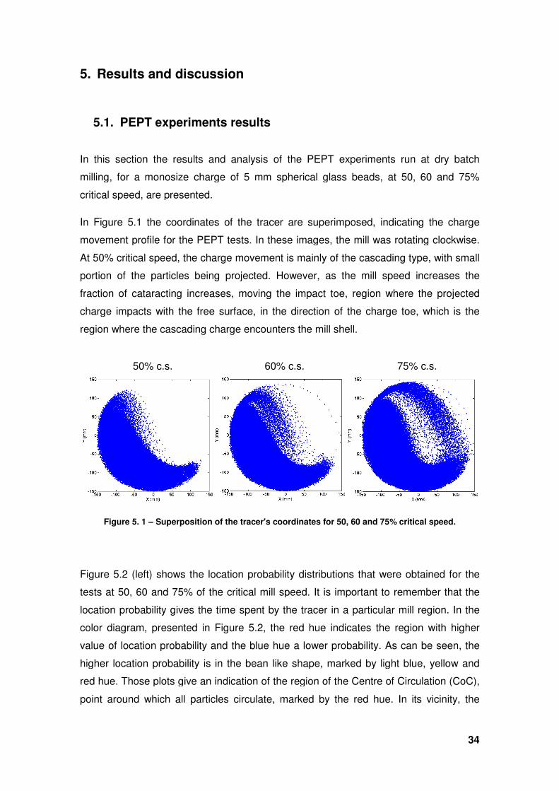
In Figure 5.1 the coordinates of the tracer are superimposed, indicating the charge

movement profile for the PEPT tests. In these images, the mill was rotating clockwise.

At 50% critical speed, the charge movement is mainly of the cascading type, with small

portion of the particles being projected. However, as the mill speed increases the

fraction of cataracting increases, moving the impact toe, region where the projected

charge impacts with the free surface, in the direction of the charge toe, which is the

region where the cascading charge encounters the mill shell.

Figure 5. 1 – Superposition of the tracer's coordinates for 50, 60 and 75% critical speed.

Figure 5.2 (left) shows the location probability distributions that were obtained for the

tests at 50, 60 and 75% of the critical mill speed. It is important to remember that the

location probability gives the time spent by the tracer in a particular mill region. I

color diagram, presented in Figure

value of location probability and the blue hue a lower probability. As can be seen, the

higher location probability is in the bean like shape, marked by light blue,

red hue. Those plots give an indication of the region of the Centre of Circulation (CoC),

point around which all particles circulate, marked by the red hue. In its vicinity, the

50% c.s.

and discussion

PEPT experiments results



critical speed, are presented.

.1 the coordinates of the tracer are superimposed, indicating the charge



f the particles being projected. However, as the mill speed increases the



re the cascading charge encounters the mill shell.

Superposition of the tracer's coordinates for 50, 60 and 75% critical speed.

2 (left) shows the location probability distributions that were obtained for the


location probability gives the time spent by the tracer in a particular mill region. I

color diagram, presented in Figure 5.2, the red hue indicates the region with higher


higher location probability is in the bean like shape, marked by light blue,



60% c.s. 75% c.s.

34



.1 the coordinates of the tracer are superimposed, indicating the charge



f the particles being projected. However, as the mill speed increases the



Superposition of the tracer's coordinates for 50, 60 and 75% critical speed.

2 (left) shows the location probability distributions that were obtained for the


location probability gives the time spent by the tracer in a particular mill region. In the

2, the red hue indicates the region with higher


higher location probability is in the bean like shape, marked by light blue, yellow and



75% c.s.

35

tracer moves more slowly, increasing the time spent in the same cell and its location

probability, marked in the plots by a red hue in the bulk charge. The region above the

bean like shape, marked by a blue hue, is mostly the cataracting region, indicating that

this region plays a smaller role on the power draw, due to its minor location probability,

as will be discussed as follows.

Another interesting feature that can be noticed in the location probability plot is thin

blue region, under the bean like shape, in the periphery. This is due to the presence of

the lifters. There are always particles in the region between them; however, the lifters

reduce their mobility making it more difficult for the tracer to occupy it.

Similar plots can be graphed for the velocity profile in the mill, as shown in Figure 5.2

(right). The charge velocity profile was determined by averaging each absolute velocity

registered for the tracer in the cells. The equilibrium surface was evident and marked

by a dark blue hue, in the velocity plot. This surface separates the ascending en-masse

charge (under the surface) from the descending charge (above the surface), making it

a region of slower movement. In contrast, the red hue in the velocity plot indicates the

region where the particles are being projected, the cataracting region. These plots

confirm that the cataracting behavior is more prominent with increasing mill speed.

Figure 5.3 reproduces the spatial plots in the form of particle distributions along the two

transversal axes, indicating the proportion of locations registered along the axes, in

relation to the total number of registered positions. Note that the center of the axis was

defined at the mill center. These distributions revealed a similar trend for the three

rotational speeds. However, as expected and can be seen by the comparisons, as the

speed increases the particles tend to move to the periphery of the mill. In the horizontal

axis, the peak height increases with increasing mill speed, indicating a larger fraction of

particles near the periphery of the mill. In contrast, in the center of the mill the fraction

of particles decreases with increasing mill speed.

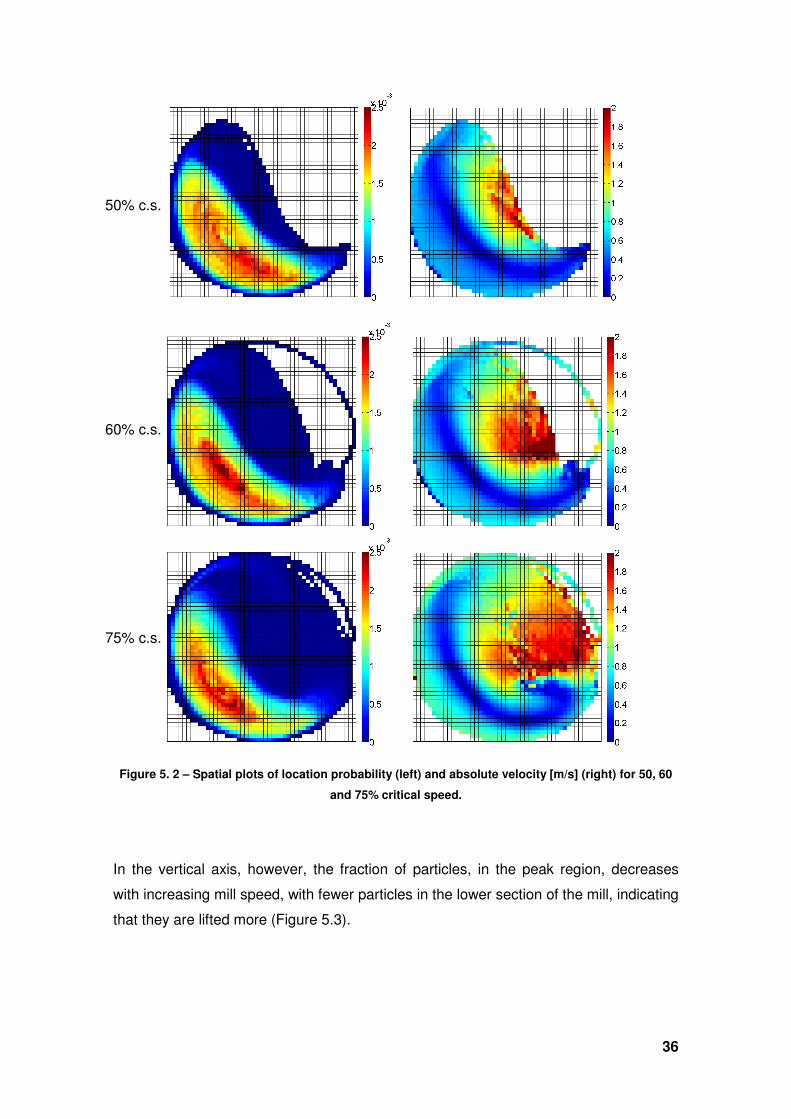
36

Figure 5. 2 – Spatial plots of location probability (left) and absolute velocity [m/s] (right) for 50, 60

and 75% critical speed.

In the vertical axis, however, the fraction of particles, in the peak region, decreases

with increasing mill speed, with fewer particles in the lower section of the mill, indicating

that they are lifted more (Figure 5.3).

50% c.s.

60% c.s.

75% c.s.

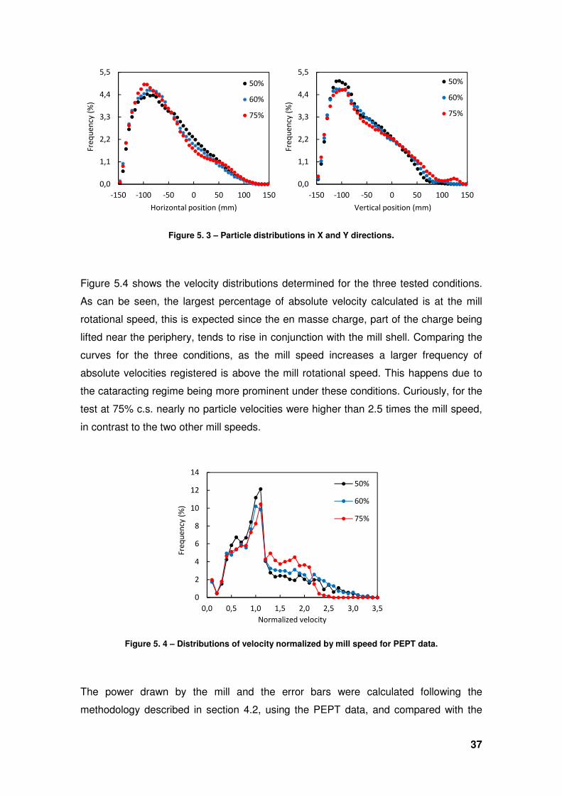
37

Figure 5. 3 – Particle distributions in X and Y directions.

Figure 5.4 shows the velocity distributions determined for the three tested conditions.

As can be seen, the largest percentage of absolute velocity calculated is at the mill

rotational speed, this is expected since the en masse charge, part of the charge being

lifted near the periphery, tends to rise in conjunction with the mill shell. Comparing the

curves for the three conditions, as the mill speed increases a larger frequency of

absolute velocities registered is above the mill rotational speed. This happens due to

the cataracting regime being more prominent under these conditions. Curiously, for the

test at 75% c.s. nearly no particle velocities were higher than 2.5 times the mill speed,

in contrast to the two other mill speeds.

Figure 5. 4 – Distributions of velocity normalized by mill speed for PEPT data.

The power drawn by the mill and the error bars were calculated following the

methodology described in section 4.2, using the PEPT data, and compared with the

0,0

1,1

2,2

3,3

4,4

5,5

-150 -100 -50 0 50 100 150

Fre

qu

en

cy (

%)


50%

60%

75%

0,0

1,1

2,2

3,3

4,4

5,5

-150 -100 -50 0 50 100 150

Fre

qu

en

cy (

%)

Vertical position (mm)

50%

60%

75%

0

2

4

6

8

10

12

14

0,0 0,5 1,0 1,5 2,0 2,5 3,0 3,5

Fre

qu

en

cy (

%)

Normalized velocity

50%

60%

75%

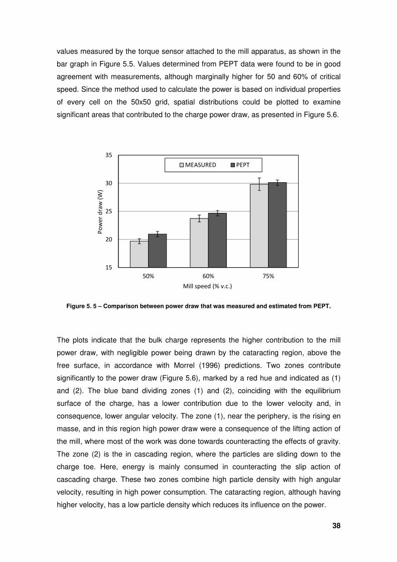
38

values measured by the torque sensor attached to the mill apparatus, as shown in the

bar graph in Figure 5.5. Values determined from PEPT data were found to be in good

agreement with measurements, although marginally higher for 50 and 60% of critical

speed. Since the method used to calculate the power is based on individual properties

of every cell on the 50x50 grid, spatial distributions could be plotted to examine

significant areas that contributed to the charge power draw, as presented in Figure 5.6.

Figure 5. 5 – Comparison between power draw that was measured and estimated from PEPT.

The plots indicate that the bulk charge represents the higher contribution to the mill

power draw, with negligible power being drawn by the cataracting region, above the

free surface, in accordance with Morrel (1996) predictions. Two zones contribute

significantly to the power draw (Figure 5.6), marked by a red hue and indicated as (1)

and (2). The blue band dividing zones (1) and (2), coinciding with the equilibrium

surface of the charge, has a lower contribution due to the lower velocity and, in

consequence, lower angular velocity. The zone (1), near the periphery, is the rising en

masse, and in this region high power draw were a consequence of the lifting action of

the mill, where most of the work was done towards counteracting the effects of gravity.

The zone (2) is the in cascading region, where the particles are sliding down to the

charge toe. Here, energy is mainly consumed in counteracting the slip action of

cascading charge. These two zones combine high particle density with high angular

velocity, resulting in high power consumption. The cataracting region, although having

higher velocity, has a low particle density which reduces its influence on the power.

15

20

25

30

35

50% 60% 75%

Po

we

r d

raw

(W

)

Mill speed (% v.c.)

MEASURED PEPT

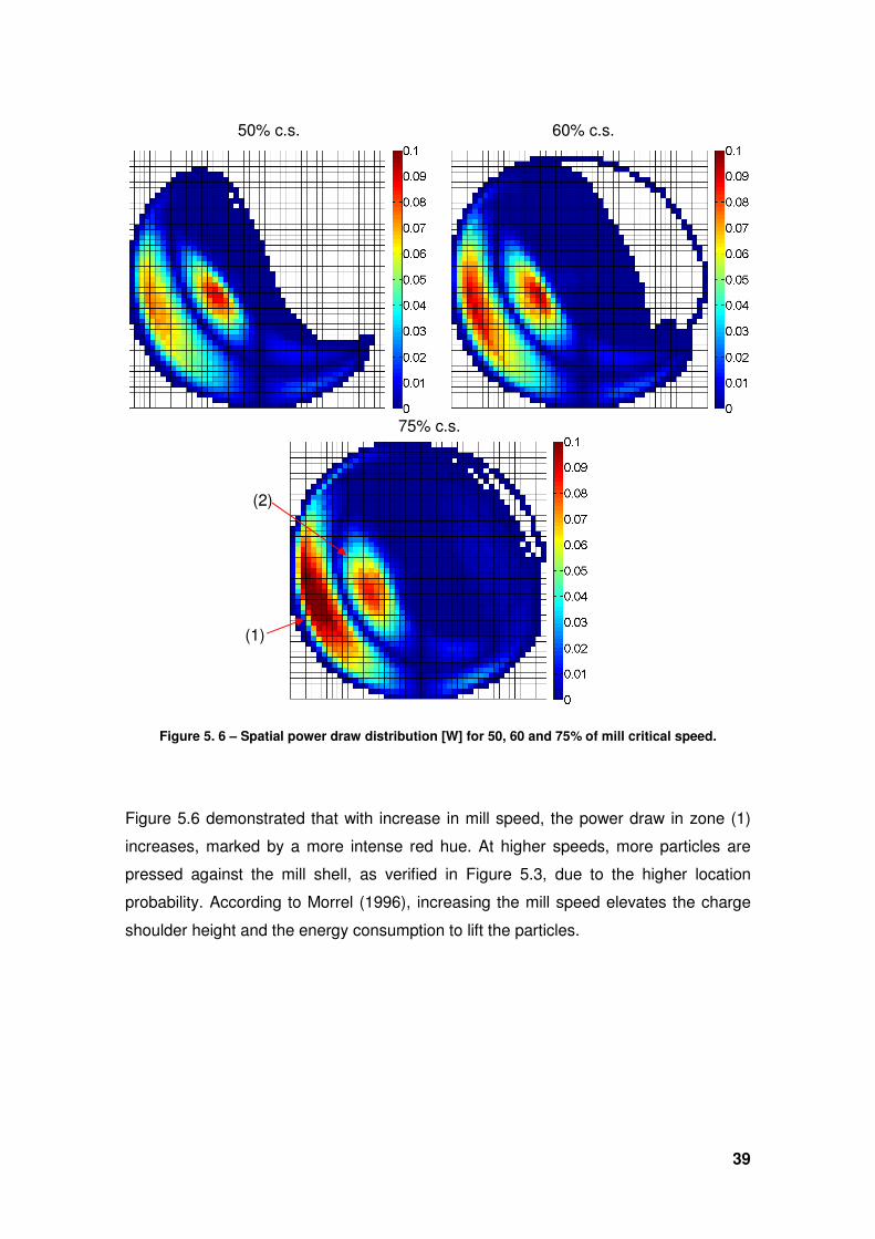
39

Figure 5. 6 – Spatial power draw distribution [W] for 50, 60 and 75% of mill critical speed.

Figure 5.6 demonstrated that with increase in mill speed, the power draw in zone (1)

increases, marked by a more intense red hue. At higher speeds, more particles are

pressed against the mill shell, as verified in Figure 5.3, due to the higher location

probability. According to Morrel (1996), increasing the mill speed elevates the charge

shoulder height and the energy consumption to lift the particles.

50% c.s. 60% c.s.

75% c.s.

(1)

(2)

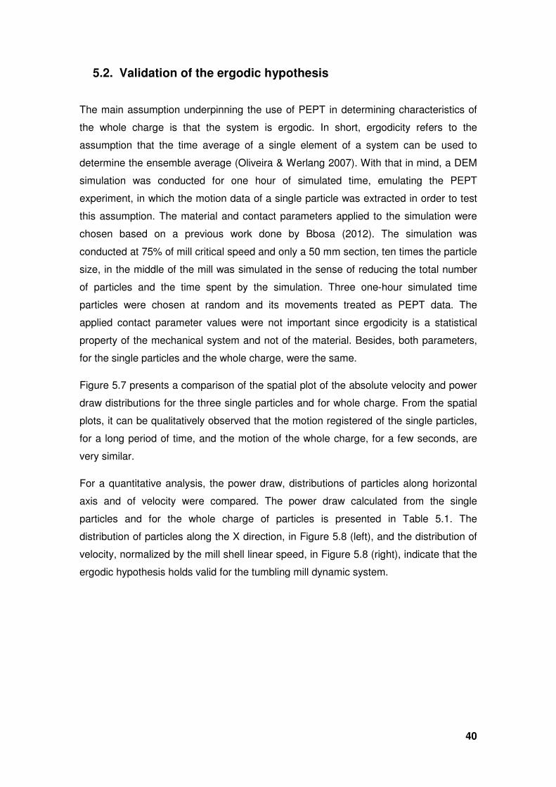
40

5.2. Validation of the ergodic hypothesis

The main assumption underpinning the use of PEPT in determining characteristics of

the whole charge is that the system is ergodic. In short, ergodicity refers to the

assumption that the time average of a single element of a system can be used to

determine the ensemble average (Oliveira & Werlang 2007). With that in mind, a DEM

simulation was conducted for one hour of simulated time, emulating the PEPT

experiment, in which the motion data of a single particle was extracted in order to test

this assumption. The material and contact parameters applied to the simulation were

chosen based on a previous work done by Bbosa (2012). The simulation was

conducted at 75% of mill critical speed and only a 50 mm section, ten times the particle

size, in the middle of the mill was simulated in the sense of reducing the total number

of particles and the time spent by the simulation. Three one-hour simulated time

particles were chosen at random and its movements treated as PEPT data. The

applied contact parameter values were not important since ergodicity is a statistical

property of the mechanical system and not of the material. Besides, both parameters,

for the single particles and the whole charge, were the same.

Figure 5.7 presents a comparison of the spatial plot of the absolute velocity and power

draw distributions for the three single particles and for whole charge. From the spatial

plots, it can be qualitatively observed that the motion registered of the single particles,

for a long period of time, and the motion of the whole charge, for a few seconds, are

very similar.

For a quantitative analysis, the power draw, distributions of particles along horizontal

axis and of velocity were compared. The power draw calculated from the single

particles and for the whole charge of particles is presented in Table 5.1. The

distribution of particles along the X direction, in Figure 5.8 (left), and the distribution of

velocity, normalized by the mill shell linear speed, in Figure 5.8 (right), indicate that the

ergodic hypothesis holds valid for the tumbling mill dynamic system.

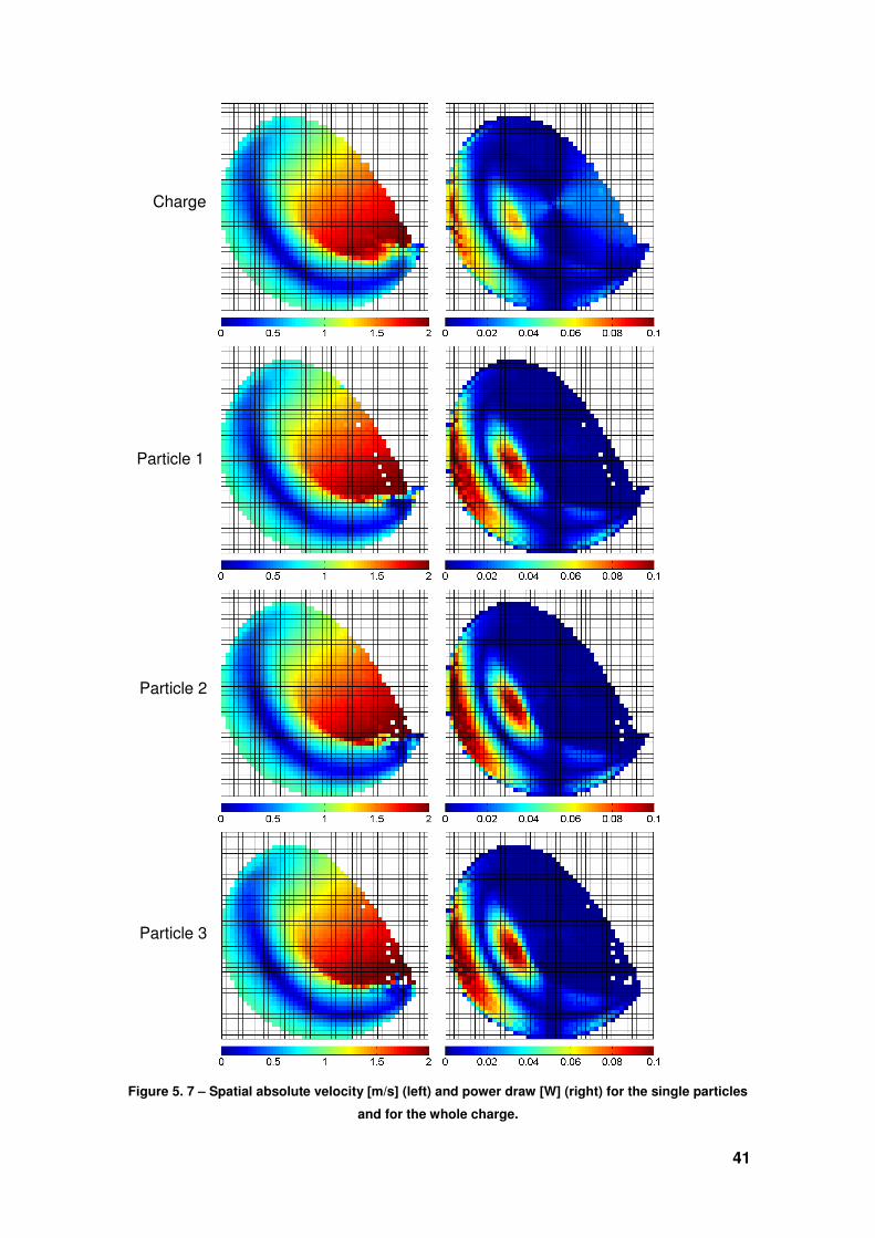
41

Figure 5. 7 – Spatial absolute velocity [m/s] (left) and power draw [W] (right) for the single particles

and for the whole charge.

Charge

Particle 1

Particle 2

Particle 3

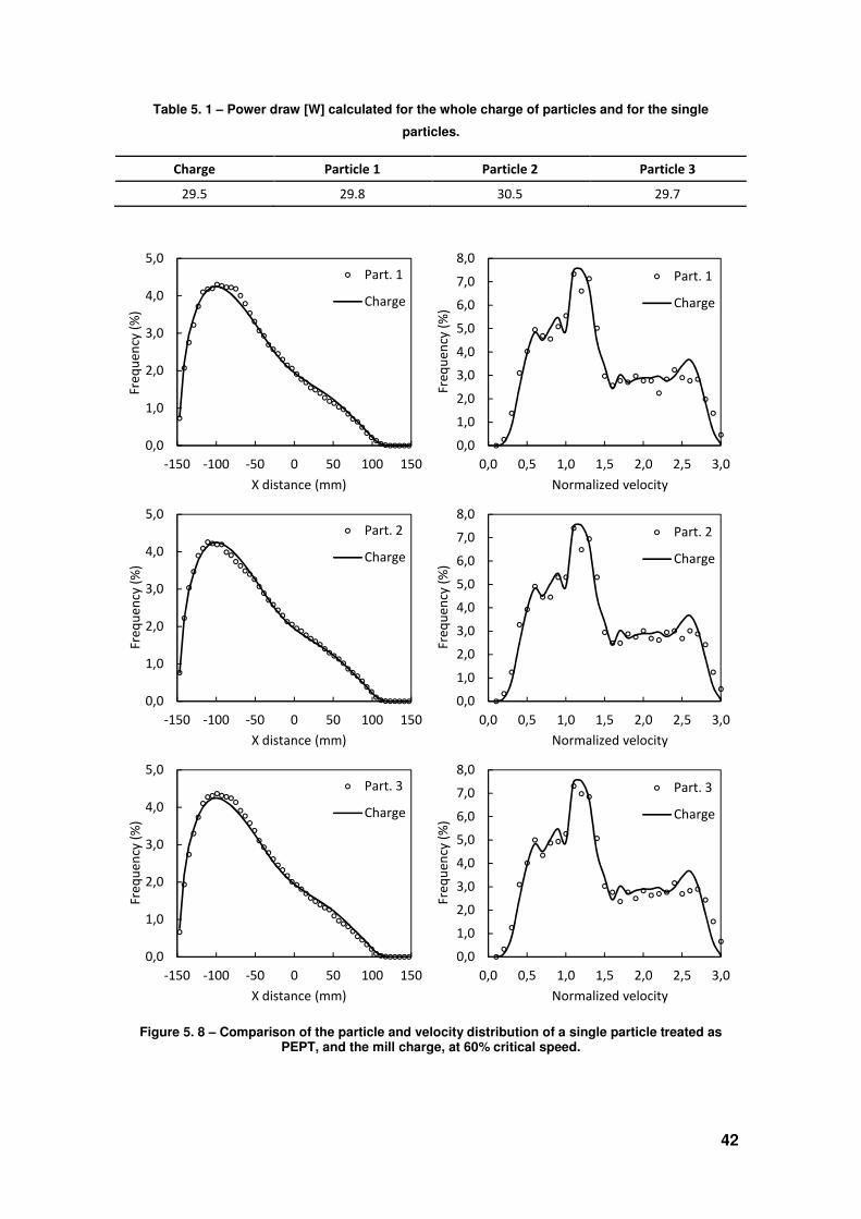
42

Table 5. 1 – Power draw [W] calculated for the whole charge of particles and for the single

particles.

Charge Particle 1 Particle 2 Particle 3

29.5 29.8 30.5 29.7

Figure 5. 8 – Comparison of the particle and velocity distribution of a single particle treated as PEPT, and the mill charge, at 60% critical speed.

0,0

1,0

2,0

3,0

4,0

5,0

-150 -100 -50 0 50 100 150

Fre

qu

en

cy (

%)

X distance (mm)

Part. 1

Charge

0,0

1,0

2,0

3,0

4,0

5,0

6,0

7,0

8,0

0,0 0,5 1,0 1,5 2,0 2,5 3,0

Fre

qu

en

cy (

%)

Normalized velocity

Part. 1

Charge

0,0

1,0

2,0

3,0

4,0

5,0

-150 -100 -50 0 50 100 150

Fre

qu

en

cy (

%)

X distance (mm)

Part. 2

Charge

0,0

1,0

2,0

3,0

4,0

5,0

6,0

7,0

8,0

0,0 0,5 1,0 1,5 2,0 2,5 3,0

Fre

qu

en

cy (

%)

Normalized velocity

Part. 2

Charge

0,0

1,0

2,0

3,0

4,0

5,0

-150 -100 -50 0 50 100 150

Fre

qu

en

cy (

%)

X distance (mm)

Part. 3

Charge

0,0

1,0

2,0

3,0

4,0

5,0

6,0

7,0

8,0

0,0 0,5 1,0 1,5 2,0 2,5 3,0

Fre

qu

en

cy (

%)

Normalized velocity

Part. 3

Charge

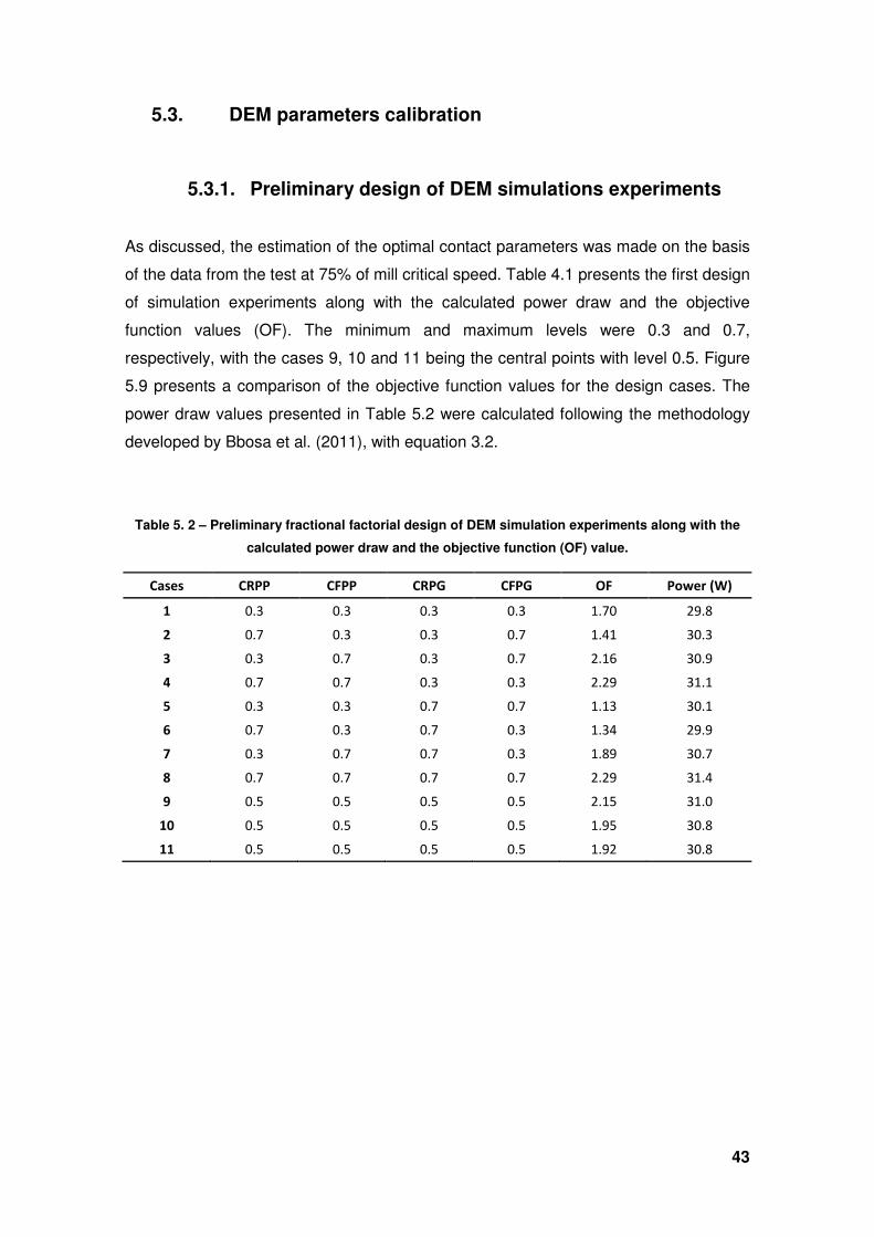
43

5.3. DEM parameters calibration

5.3.1. Preliminary design of DEM simulations experiments

As discussed, the estimation of the optimal contact parameters was made on the basis

of the data from the test at 75% of mill critical speed. Table 4.1 presents the first design

of simulation experiments along with the calculated power draw and the objective

function values (OF). The minimum and maximum levels were 0.3 and 0.7,

respectively, with the cases 9, 10 and 11 being the central points with level 0.5. Figure

5.9 presents a comparison of the objective function values for the design cases. The

power draw values presented in Table 5.2 were calculated following the methodology

developed by Bbosa et al. (2011), with equation 3.2.

Table 5. 2 – Preliminary fractional factorial design of DEM simulation experiments along with the

calculated power draw and the objective function (OF) value.

Cases CRPP CFPP CRPG CFPG OF Power (W)

1 0.3 0.3 0.3 0.3 1.70 29.8

2 0.7 0.3 0.3 0.7 1.41 30.3

3 0.3 0.7 0.3 0.7 2.16 30.9

4 0.7 0.7 0.3 0.3 2.29 31.1

5 0.3 0.3 0.7 0.7 1.13 30.1

6 0.7 0.3 0.7 0.3 1.34 29.9

7 0.3 0.7 0.7 0.3 1.89 30.7

8 0.7 0.7 0.7 0.7 2.29 31.4

9 0.5 0.5 0.5 0.5 2.15 31.0

10 0.5 0.5 0.5 0.5 1.95 30.8

11 0.5 0.5 0.5 0.5 1.92 30.8

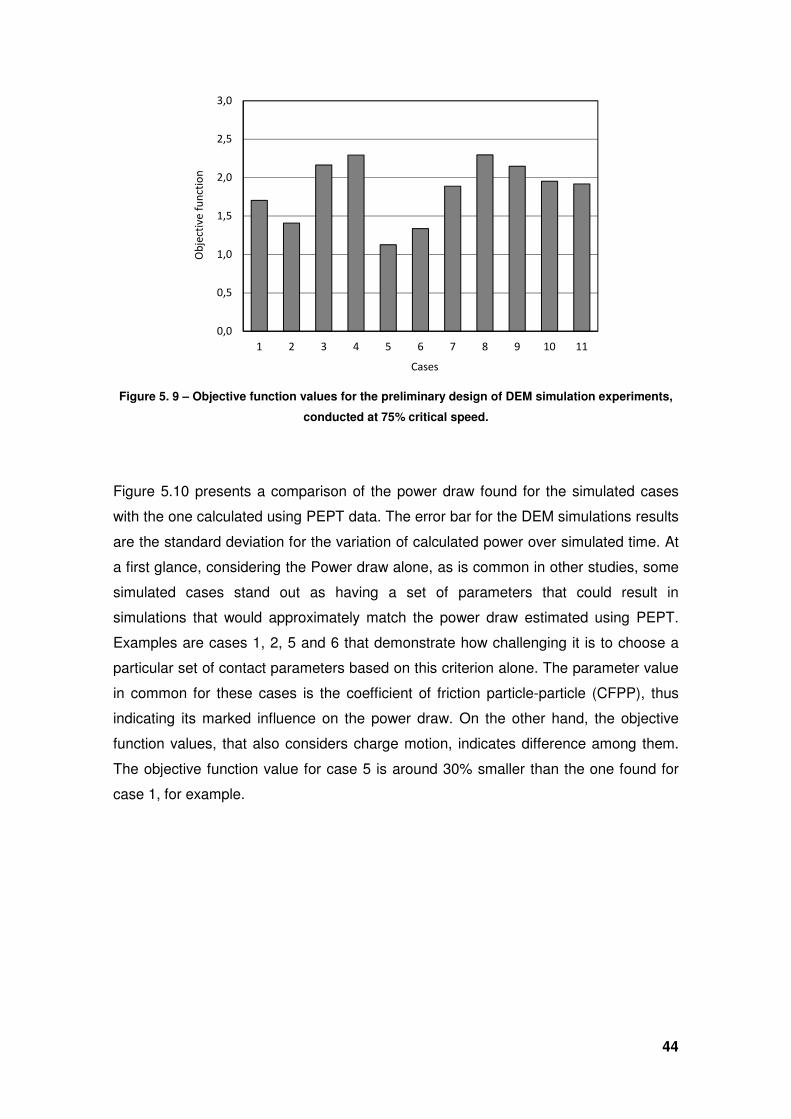
44

Figure 5. 9 – Objective function values for the preliminary design of DEM simulation experiments,

conducted at 75% critical speed.

Figure 5.10 presents a comparison of the power draw found for the simulated cases

with the one calculated using PEPT data. The error bar for the DEM simulations results

are the standard deviation for the variation of calculated power over simulated time. At

a first glance, considering the Power draw alone, as is common in other studies, some

simulated cases stand out as having a set of parameters that could result in

simulations that would approximately match the power draw estimated using PEPT.

Examples are cases 1, 2, 5 and 6 that demonstrate how challenging it is to choose a

particular set of contact parameters based on this criterion alone. The parameter value

in common for these cases is the coefficient of friction particle-particle (CFPP), thus

indicating its marked influence on the power draw. On the other hand, the objective

function values, that also considers charge motion, indicates difference among them.

The objective function value for case 5 is around 30% smaller than the one found for

case 1, for example.

0,0

0,5

1,0

1,5

2,0

2,5

3,0

1 2 3 4 5 6 7 8 9 10 11

Ob

ject

ive

fu

nct

ion

Cases

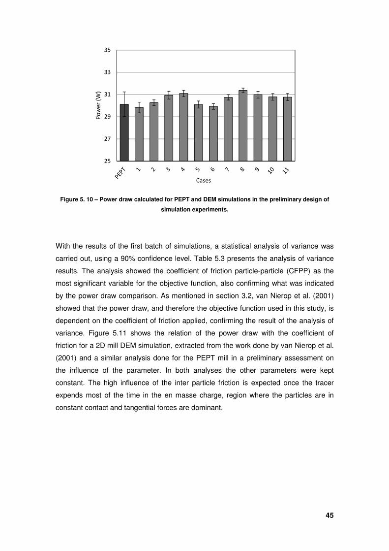
45

Figure 5. 10 – Power draw calculated for PEPT and DEM simulations in the preliminary design of

simulation experiments.

With the results of the first batch of simulations, a statistical analysis of variance was

carried out, using a 90% confidence level. Table 5.3 presents the analysis of variance

results. The analysis showed the coefficient of friction particle-particle (CFPP) as the

most significant variable for the objective function, also confirming what was indicated

by the power draw comparison. As mentioned in section 3.2, van Nierop et al. (2001)

showed that the power draw, and therefore the objective function used in this study, is

dependent on the coefficient of friction applied, confirming the result of the analysis of

variance. Figure 5.11 shows the relation of the power draw with the coefficient of

friction for a 2D mill DEM simulation, extracted from the work done by van Nierop et al.

(2001) and a similar analysis done for the PEPT mill in a preliminary assessment on

the influence of the parameter. In both analyses the other parameters were kept

constant. The high influence of the inter particle friction is expected once the tracer

expends most of the time in the en masse charge, region where the particles are in

constant contact and tangential forces are dominant.

25

27

29

31

33

35

Po

we

r (W

)

Cases

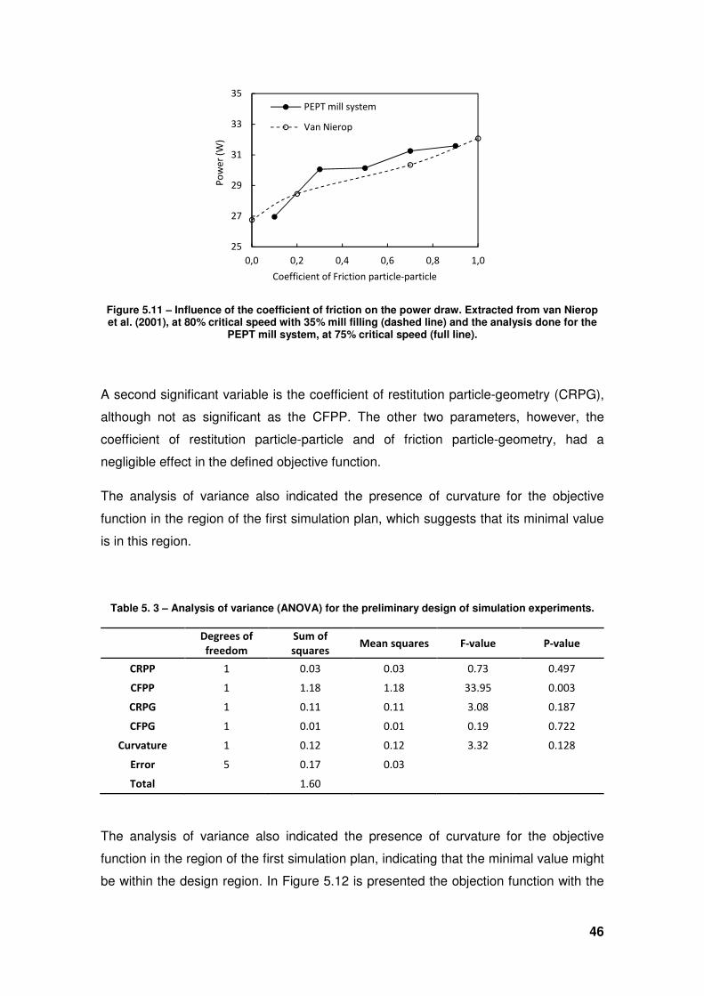
46

Figure 5.11 – Influence of the coefficient of friction on the power draw. Extracted from van Nierop et al. (2001), at 80% critical speed with 35% mill filling (dashed line) and the analysis done for the

PEPT mill system, at 75% critical speed (full line).

A second significant variable is the coefficient of restitution particle-geometry (CRPG),

although not as significant as the CFPP. The other two parameters, however, the

coefficient of restitution particle-particle and of friction particle-geometry, had a

negligible effect in the defined objective function.

The analysis of variance also indicated the presence of curvature for the objective

function in the region of the first simulation plan, which suggests that its minimal value

is in this region.

Table 5. 3 – Analysis of variance (ANOVA) for the preliminary design of simulation experiments.

Degrees of

freedom

Sum of

squares Mean squares F-value P-value

CRPP 1 0.03 0.03 0.73 0.497

CFPP 1 1.18 1.18 33.95 0.003

CRPG 1 0.11 0.11 3.08 0.187

CFPG 1 0.01 0.01 0.19 0.722

Curvature 1 0.12 0.12 3.32 0.128

Error 5 0.17 0.03

Total 1.60

The analysis of variance also indicated the presence of curvature for the objective

function in the region of the first simulation plan, indicating that the minimal value might

be within the design region. In Figure 5.12 is presented the objection function with the

25

27

29

31

33

35

0,0 0,2 0,4 0,6 0,8 1,0

Po

we

r (W

)

Coefficient of Friction particle-particle

PEPT mill system

Van Nierop

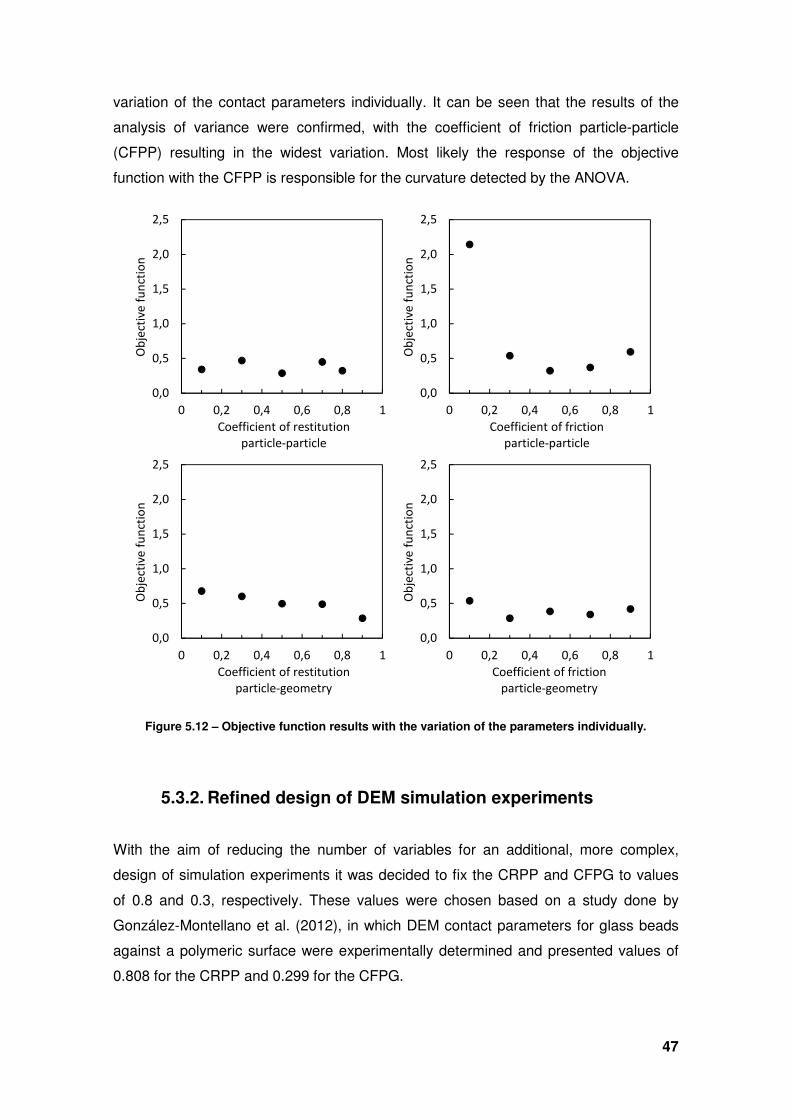
47

variation of the contact parameters individually. It can be seen that the results of the

analysis of variance were confirmed, with the coefficient of friction particle-particle

(CFPP) resulting in the widest variation. Most likely the response of the objective

function with the CFPP is responsible for the curvature detected by the ANOVA.

Figure 5.12 – Objective function results with the variation of the parameters individually.

5.3.2. Refined design of DEM simulation experiments

With the aim of reducing the number of variables for an additional, more complex,

design of simulation experiments it was decided to fix the CRPP and CFPG to values

of 0.8 and 0.3, respectively. These values were chosen based on a study done by

González-Montellano et al. (2012), in which DEM contact parameters for glass beads

against a polymeric surface were experimentally determined and presented values of

0.808 for the CRPP and 0.299 for the CFPG.

0,0

0,5

1,0

1,5

2,0

2,5

0 0,2 0,4 0,6 0,8 1

Ob

ject

ive

fu

nct

ion

Coefficient of restitution

particle-particle

0,0

0,5

1,0

1,5

2,0

2,5

0 0,2 0,4 0,6 0,8 1O

bje

ctiv

e f

un

ctio

n

Coefficient of friction

particle-particle

0,0

0,5

1,0

1,5

2,0

2,5

0 0,2 0,4 0,6 0,8 1

Ob

ject

ive

fu

nct

ion

Coefficient of restitution

particle-geometry

0,0

0,5

1,0

1,5

2,0

2,5

0 0,2 0,4 0,6 0,8 1

Ob

ject

ive

fu

nct

ion

Coefficient of friction

particle-geometry

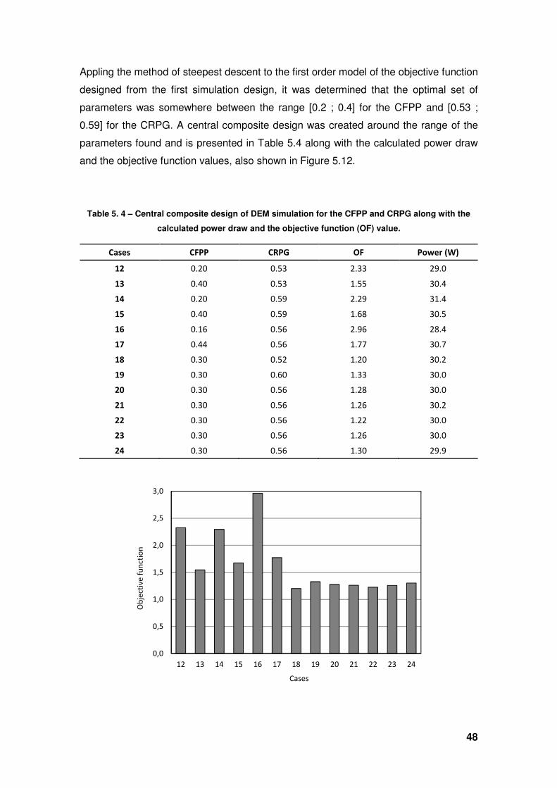
48

Appling the method of steepest descent to the first order model of the objective function

designed from the first simulation design, it was determined that the optimal set of

parameters was somewhere between the range [0.2 ; 0.4] for the CFPP and [0.53 ;

0.59] for the CRPG. A central composite design was created around the range of the

parameters found and is presented in Table 5.4 along with the calculated power draw

and the objective function values, also shown in Figure 5.12.

Table 5. 4 – Central composite design of DEM simulation for the CFPP and CRPG along with the

calculated power draw and the objective function (OF) value.

Cases CFPP CRPG OF Power (W)

12 0.20 0.53 2.33 29.0

13 0.40 0.53 1.55 30.4

14 0.20 0.59 2.29 31.4

15 0.40 0.59 1.68 30.5

16 0.16 0.56 2.96 28.4

17 0.44 0.56 1.77 30.7

18 0.30 0.52 1.20 30.2

19 0.30 0.60 1.33 30.0

20 0.30 0.56 1.28 30.0

21 0.30 0.56 1.26 30.2

22 0.30 0.56 1.22 30.0

23 0.30 0.56 1.26 30.0

24 0.30 0.56 1.30 29.9

0,0

0,5

1,0

1,5

2,0

2,5

3,0

12 13 14 15 16 17 18 19 20 21 22 23 24

Ob

ject

ive

fu

nct

ion

Cases

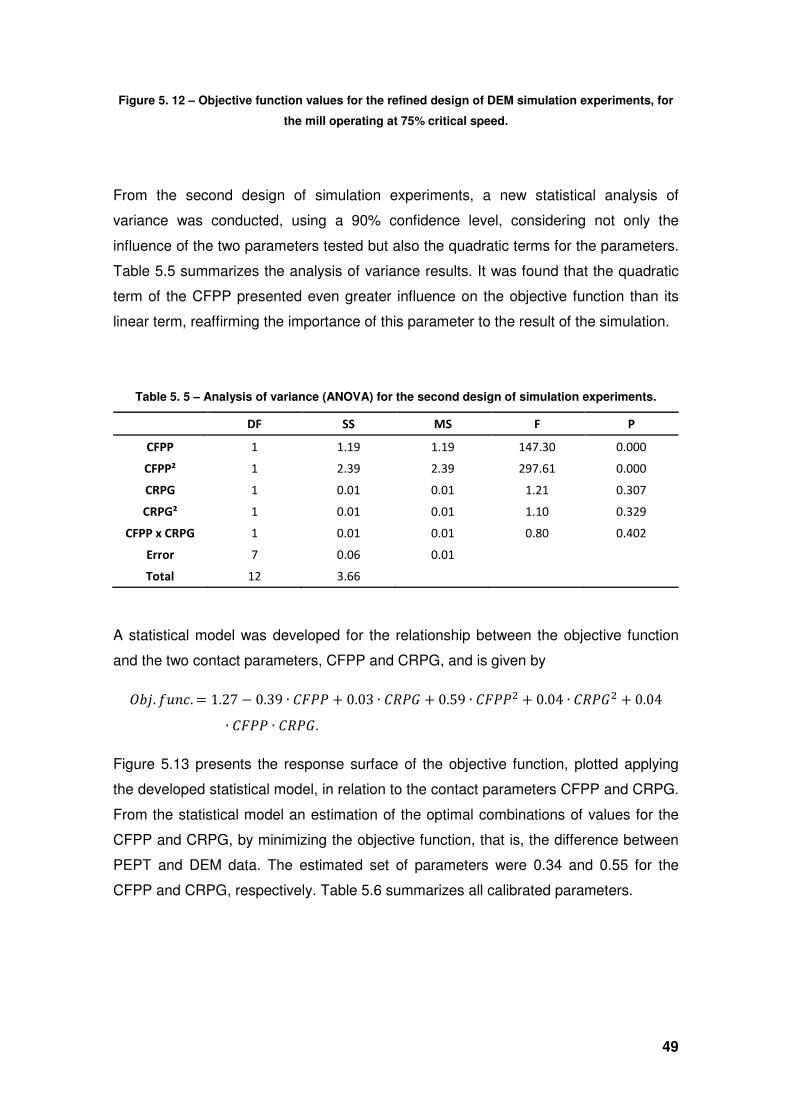
49

Figure 5. 12 – Objective function values for the refined design of DEM simulation experiments, for

the mill operating at 75% critical speed.

From the second design of simulation experiments, a new statistical analysis of

variance was conducted, using a 90% confidence level, considering not only the

influence of the two parameters tested but also the quadratic terms for the parameters.

Table 5.5 summarizes the analysis of variance results. It was found that the quadratic

term of the CFPP presented even greater influence on the objective function than its

linear term, reaffirming the importance of this parameter to the result of the simulation.

Table 5. 5 – Analysis of variance (ANOVA) for the second design of simulation experiments.

DF SS MS F P

CFPP 1 1.19 1.19 147.30 0.000

CFPP² 1 2.39 2.39 297.61 0.000

CRPG 1 0.01 0.01 1.21 0.307

CRPG² 1 0.01 0.01 1.10 0.329

CFPP x CRPG 1 0.01 0.01 0.80 0.402

Error 7 0.06 0.01

Total 12 3.66

A statistical model was developed for the relationship between the objective function

and the two contact parameters, CFPP and CRPG, and is given by

yzb. I{^�. = 1.27 − 0.39 ∙ �G�� + 0.03 ∙ �U�� + 0.59 ∙ �G��, + 0.04 ∙ �U��, + 0.04∙ �G�� ∙ �U��. Figure 5.13 presents the response surface of the objective function, plotted applying

the developed statistical model, in relation to the contact parameters CFPP and CRPG.

From the statistical model an estimation of the optimal combinations of values for the

CFPP and CRPG, by minimizing the objective function, that is, the difference between

PEPT and DEM data. The estimated set of parameters were 0.34 and 0.55 for the

CFPP and CRPG, respectively. Table 5.6 summarizes all calibrated parameters.

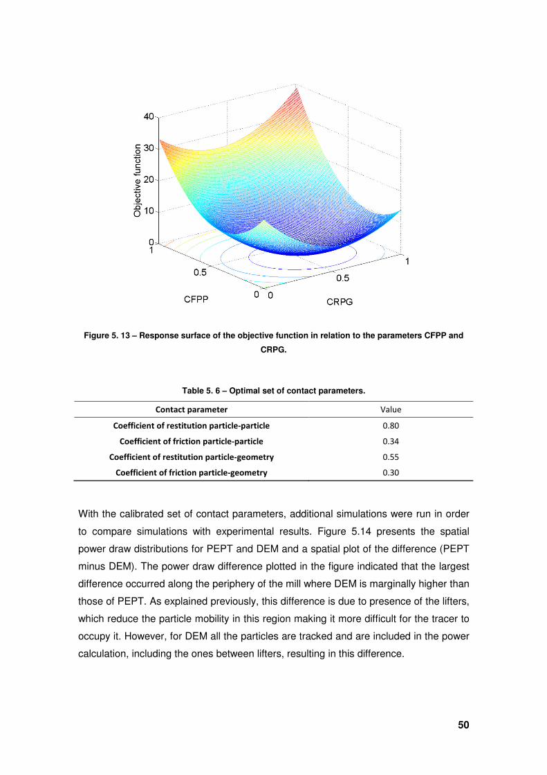
50

Figure 5. 13 – Response surface of the objective function in relation to the parameters CFPP and

CRPG.

Table 5. 6 – Optimal set of contact parameters.

Contact parameter Value

Coefficient of restitution particle-particle 0.80

Coefficient of friction particle-particle 0.34

Coefficient of restitution particle-geometry 0.55

Coefficient of friction particle-geometry 0.30

With the calibrated set of contact parameters, additional simulations were run in order

to compare simulations with experimental results. Figure 5.14 presents the spatial

power draw distributions for PEPT and DEM and a spatial plot of the difference (PEPT

minus DEM). The power draw difference plotted in the figure indicated that the largest

difference occurred along the periphery of the mill where DEM is marginally higher than

those of PEPT. As explained previously, this difference is due to presence of the lifters,

which reduce the particle mobility in this region making it more difficult for the tracer to

occupy it. However, for DEM all the particles are tracked and are included in the power

calculation, including the ones between lifters, resulting in this difference.

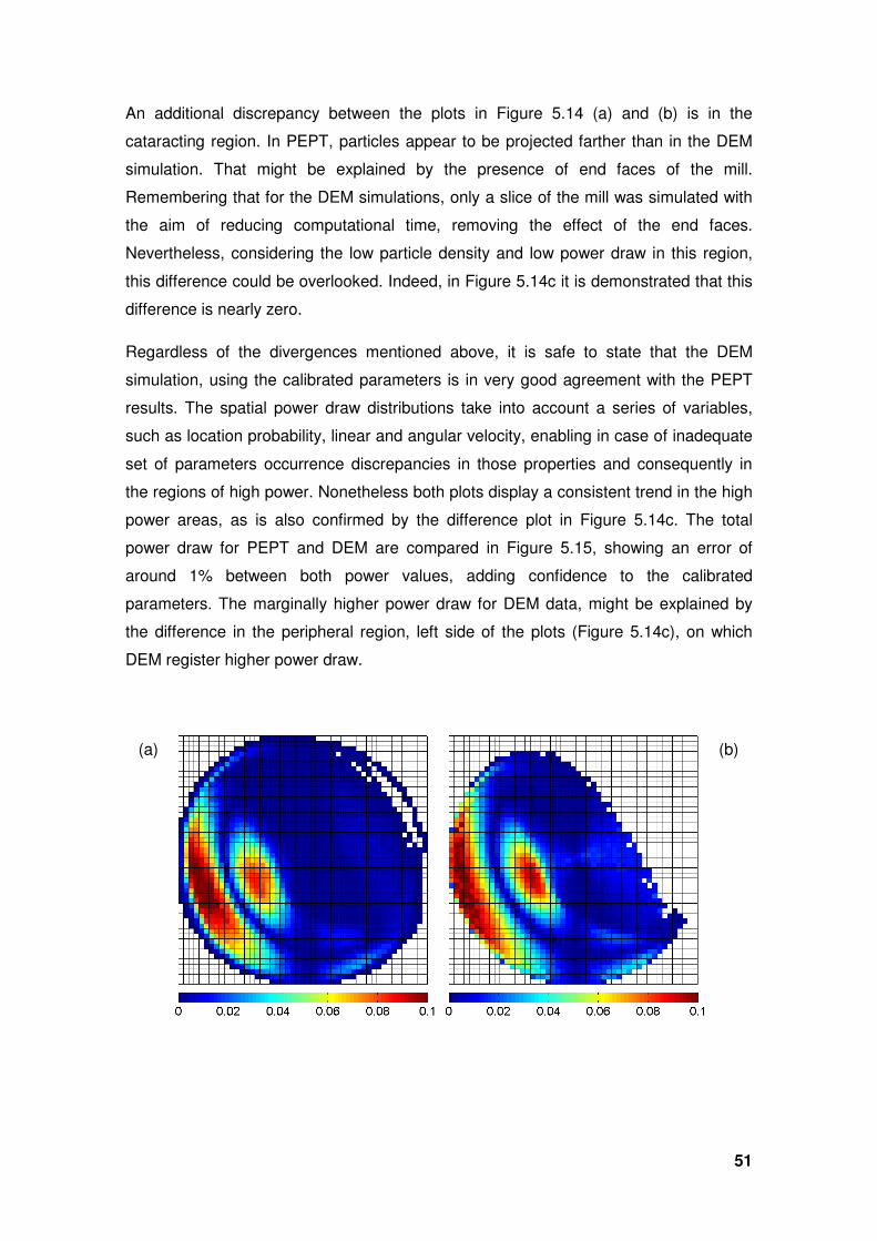
51

An additional discrepancy between the plots in Figure 5.14 (a) and (b) is in the

cataracting region. In PEPT, particles appear to be projected farther than in the DEM

simulation. That might be explained by the presence of end faces of the mill.

Remembering that for the DEM simulations, only a slice of the mill was simulated with

the aim of reducing computational time, removing the effect of the end faces.

Nevertheless, considering the low particle density and low power draw in this region,

this difference could be overlooked. Indeed, in Figure 5.14c it is demonstrated that this

difference is nearly zero.

Regardless of the divergences mentioned above, it is safe to state that the DEM

simulation, using the calibrated parameters is in very good agreement with the PEPT

results. The spatial power draw distributions take into account a series of variables,

such as location probability, linear and angular velocity, enabling in case of inadequate

set of parameters occurrence discrepancies in those properties and consequently in

the regions of high power. Nonetheless both plots display a consistent trend in the high

power areas, as is also confirmed by the difference plot in Figure 5.14c. The total

power draw for PEPT and DEM are compared in Figure 5.15, showing an error of

around 1% between both power values, adding confidence to the calibrated

parameters. The marginally higher power draw for DEM data, might be explained by

the difference in the peripheral region, left side of the plots (Figure 5.14c), on which

DEM register higher power draw.

(a) (b)

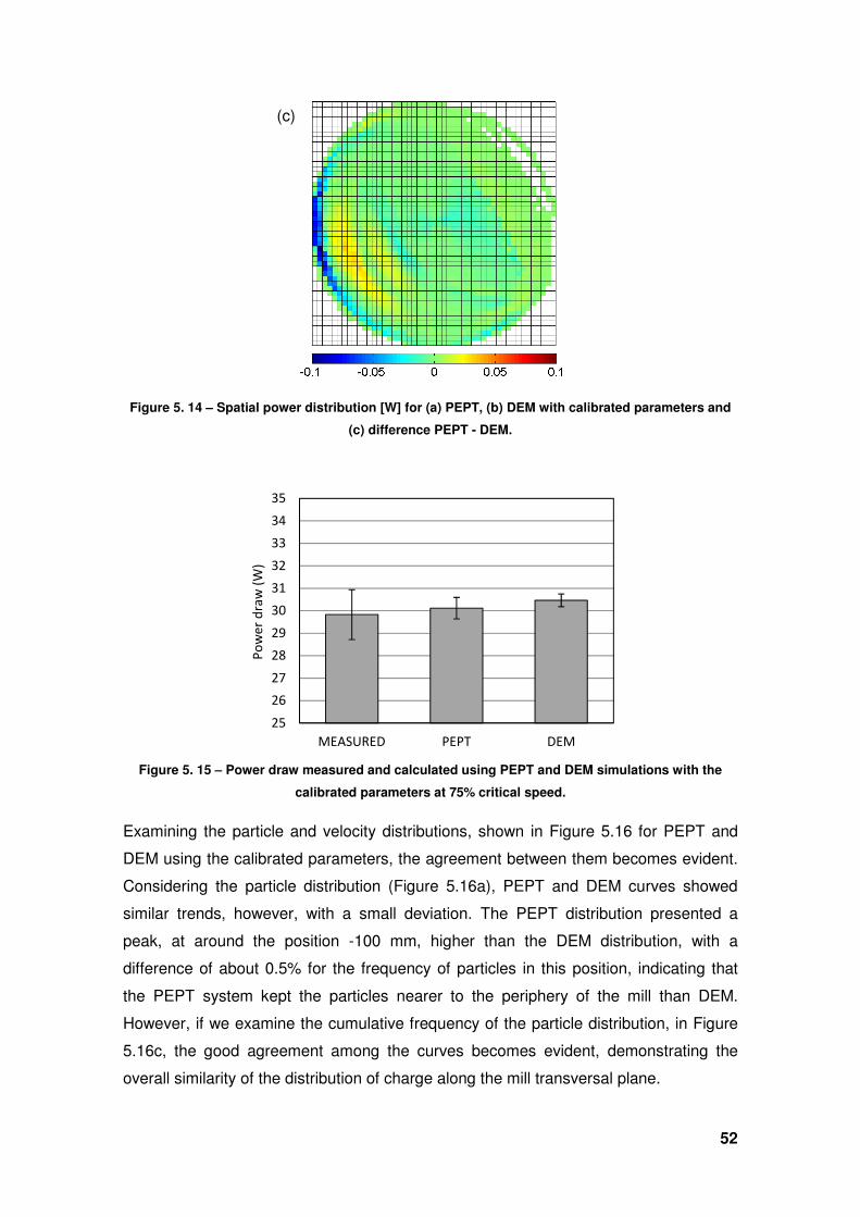
52

Figure 5. 14 – Spatial power distribution [W] for (a) PEPT, (b) DEM with calibrated parameters and

(c) difference PEPT - DEM.

Figure 5. 15 – Power draw measured and calculated using PEPT and DEM simulations with the

calibrated parameters at 75% critical speed.

Examining the particle and velocity distributions, shown in Figure 5.16 for PEPT and

DEM using the calibrated parameters, the agreement between them becomes evident.

Considering the particle distribution (Figure 5.16a), PEPT and DEM curves showed

similar trends, however, with a small deviation. The PEPT distribution presented a

peak, at around the position -100 mm, higher than the DEM distribution, with a

difference of about 0.5% for the frequency of particles in this position, indicating that

the PEPT system kept the particles nearer to the periphery of the mill than DEM.

However, if we examine the cumulative frequency of the particle distribution, in Figure

5.16c, the good agreement among the curves becomes evident, demonstrating the

overall similarity of the distribution of charge along the mill transversal plane.

25

26

27

28

29

30

31

32

33

34

35

MEASURED PEPT DEM

Po

we

r d

raw

(W

)

(c)

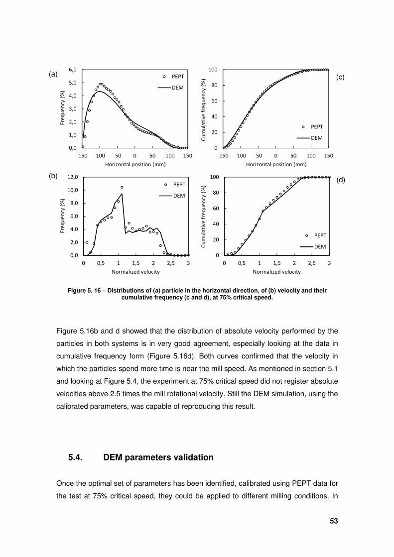
53

Figure 5. 16 – Distributions of (a) particle in the horizontal direction, of (b) velocity and their cumulative frequency (c and d), at 75% critical speed.

Figure 5.16b and d showed that the distribution of absolute velocity performed by the

particles in both systems is in very good agreement, especially looking at the data in

cumulative frequency form (Figure 5.16d). Both curves confirmed that the velocity in

which the particles spend more time is near the mill speed. As mentioned in section 5.1

and looking at Figure 5.4, the experiment at 75% critical speed did not register absolute

velocities above 2.5 times the mill rotational velocity. Still the DEM simulation, using the

calibrated parameters, was capable of reproducing this result.

5.4. DEM parameters validation

Once the optimal set of parameters has been identified, calibrated using PEPT data for

the test at 75% critical speed, they could be applied to different milling conditions. In

0,0

1,0

2,0

3,0

4,0

5,0

6,0

-150 -100 -50 0 50 100 150

Fre

qu

en

cy (

%)


PEPT

DEM

0

20

40

60

80

100

-150 -100 -50 0 50 100 150

Cu

mu

lati

ve

fre

qu

en

cy (

%)


PEPT

DEM

0,0

2,0

4,0

6,0

8,0

10,0

12,0

0 0,5 1 1,5 2 2,5 3

Fre

qu

en

cy (

%)

Normalized velocity

PEPT

DEM

0

20

40

60

80

100

0 0,5 1 1,5 2 2,5 3

Cu

mu

lati

ve

fre

qu

en

cy (

%)

Normalized velocity

PEPT

DEM

(a)

(b)

(c)

(d)

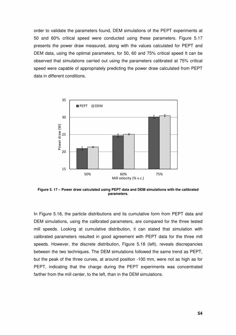
54

order to validate the parameters found, DEM simulations of the PEPT experiments at

50 and 60% critical speed were conducted using these parameters. Figure 5.17

presents the power draw measured, along with the values calculated for PEPT and

DEM data, using the optimal parameters, for 50, 60 and 75% critical speed It can be

observed that simulations carried out using the parameters calibrated at 75% critical

speed were capable of appropriately predicting the power draw calculated from PEPT

data in different conditions.

Figure 5. 17 – Power draw calculated using PEPT data and DEM simulations with the calibrated parameters.

In Figure 5.18, the particle distributions and its cumulative form from PEPT data and

DEM simulations, using the calibrated parameters, are compared for the three tested

mill speeds. Looking at cumulative distribution, it can stated that simulation with

calibrated parameters resulted in good agreement with PEPT data for the three mill

speeds. However, the discrete distribution, Figure 5.18 (left), reveals discrepancies

between the two techniques. The DEM simulations followed the same trend as PEPT,

but the peak of the three curves, at around position -100 mm, were not as high as for

PEPT, indicating that the charge during the PEPT experiments was concentrated

farther from the mill center, to the left, than in the DEM simulations.

15

20

25

30

35

50% 60% 75%

Po

we

r d

raw

(W

)

Mill velocity (% v.c.)

PEPT DEM

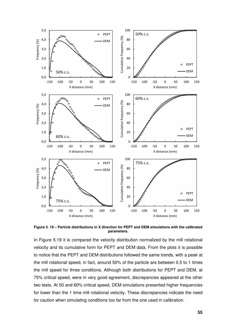
55

Figure 5. 18 – Particle distributions in X direction for PEPT and DEM simulations with the calibrated parameters.

In Figure 5.19 it is compared the velocity distribution normalized by the mill rotational

velocity and its cumulative form for PEPT and DEM data. From the plots it is possible

to notice that the PEPT and DEM distributions followed the same trends, with a peak at

the mill rotational speed, in fact, around 50% of the particle are between 0.5 to 1 times

the mill speed for three conditions. Although both distributions for PEPT and DEM, at

75% critical speed, were in very good agreement, discrepancies appeared at the other

two tests. At 50 and 60% critical speed, DEM simulations presented higher frequencies

for lower than the 1 time mill rotational velocity. These discrepancies indicate the need

for caution when simulating conditions too far from the one used in calibration.

0,0

1,0

2,0

3,0

4,0

5,0

-150 -100 -50 0 50 100 150

Fre

qu

en

cy (

%)

X distance (mm)

50% c.s.

PEPT

DEM

0

20

40

60

80

100

-150 -100 -50 0 50 100 150

Cu

mu

lati

ve

fre

qu

en

cy (

%)

X distance (mm)

50% c.s.

PEPT

DEM

0,0

1,0

2,0

3,0

4,0

5,0

-150 -100 -50 0 50 100 150

Fre

qu

en

cy (

%)

X distance (mm)

60% c.s.

PEPT

DEM

0

20

40

60

80

100

-150 -100 -50 0 50 100 150

Cu

mu

lati

ve

fre

qu

en

cy (

%)

X distance (mm)

60% c.s.

PEPT

DEM

0,0

1,0

2,0

3,0

4,0

5,0

-150 -100 -50 0 50 100 150

Fre

qu

en

cy (

%)

X distance (mm)

75% c.s.

PEPT

DEM

0

20

40

60

80

100

-150 -100 -50 0 50 100 150

Cu

mu

lati

ve

fre

qu

en

cy (

%)

X distance (mm)

75% c.s.

PEPT

DEM

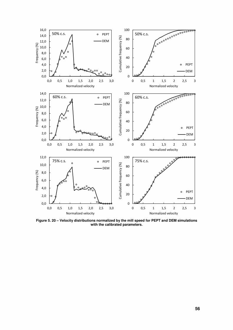
56

Figure 5. 20 – Velocity distributions normalized by the mill speed for PEPT and DEM simulations with the calibrated parameters.

0,0

2,0

4,0

6,0

8,0

10,0

12,0

14,0

16,0

0,0 0,5 1,0 1,5 2,0 2,5 3,0

Fre

qu

en

cy (

%)

Normalized velocity

50% c.s. PEPT

DEM

0

20

40

60

80

100

0 0,5 1 1,5 2 2,5 3

Cu

mu

lati

ve

fre

qu

en

cy (

%)

Normalized velocity

50% c.s.

PEPT

DEM

0,0

2,0

4,0

6,0

8,0

10,0

12,0

14,0

0,0 0,5 1,0 1,5 2,0 2,5 3,0

Fre

qu

en

cy (

%)

Normalized velocity

60% c.s. PEPT

DEM

0

20

40

60

80

100

0 0,5 1 1,5 2 2,5 3

Cu

mu

lati

ve

fre

qu

en

cy (

%)

Normalized velocity

60% c.s.

PEPT

DEM

0,0

2,0

4,0

6,0

8,0

10,0

12,0

0,0 0,5 1,0 1,5 2,0 2,5 3,0

Fre

qu

en

cy (

%)

Normalized velocity

75% c.s. PEPT

DEM

0

20

40

60

80

100

0 0,5 1 1,5 2 2,5 3

Cu

mu

lati

ve

fre

qu

en

cy (

%)

Normalized velocity

75% c.s.

PEPT

DEM

57

6. Conclusions

The scope of this work was guided on the hypothesis the effect of operational

conditions on charge movement in a tumbling mill could be quantified using data from

PEPT. Evidence on the veracity of this hypothesis was obtained through DEM

simulation emulating the PEPT experiment.

PEPT experiments were then conducted using dry glass bead charge of 5 mm in a

laboratory scale tumbling mill, in the mill speeds of 50, 60 and 75% of the critical

speed. The statistical properties from these tests were used for calibration and

validation of DEM contact parameters, carried out using an identical mill geometry and

charge. Data from these two approaches was used to determine and comparer the

charge power, mass distribution throughout the mill projection plane and velocity

distribution.

The assumed hypothesis was confirmed based on the following conclusions:

• Power draw values calculated from PEPT data were similar with power

measured directly during the experiments, although marginally higher for 50 and

60% of critical speed.

• DEM simulation tracking the movement of a single particle for one hour of

simulated time resulted in very good agreement between single particle and

complete charge when comparing spatial plots of absolute velocity and power

draw.

• The similarity for the particle distribution along the mill projection plane and

normalized velocity distribution were an additional evidence of the validity of the

ergodic hypothesis.

On the influence of parameters, it was observed that the coefficient of friction between

grinding media in DEM has a great influence on the power consumption, which is

expected considering that for condition with mill speed under 100% c.s., for the largest

part of the time, particles are only in contact with other particles. Additionally, the

adopted method for determining power draw looks in the point of view of the particles,

instead of the mill geometry, revealing the influence of particle interaction. On the other

hand, the coefficient of friction between particles and the mill shell was found irrelevant

to charge motion, what is also expected once most of the particles in direct contact with

the mill walls hardly slip and are dragged, by action of the lifters, along with it.

Although the contact parameters found by the calibration responded satisfactorily in the

three tested conditions and overall tendencies for particle and velocity distribution were

58

similar, some discrepancies were verified. It is also important to notice that no set of

parameters tested was able compare perfectly to the PEPT distributions, being the

ones chosen as optimal the closest approximation. Even so, the optimal set of contact

parameters, found by the calibration can provide good approximation for different

milling conditions, such as different mill speed, filling, geometry and particle size

distribution.

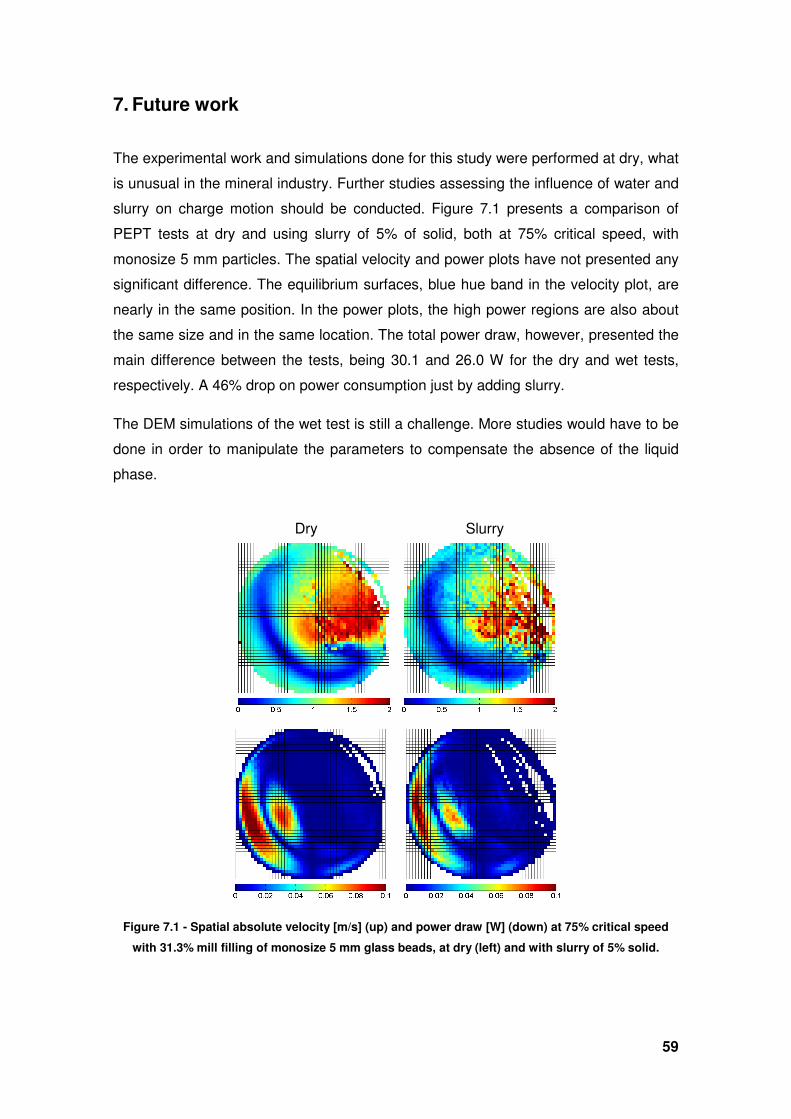
59

7. Future work

The experimental work and simulations done for this study were performed at dry, what

is unusual in the mineral industry. Further studies assessing the influence of water and

slurry on charge motion should be conducted. Figure 7.1 presents a comparison of

PEPT tests at dry and using slurry of 5% of solid, both at 75% critical speed, with

monosize 5 mm particles. The spatial velocity and power plots have not presented any

significant difference. The equilibrium surfaces, blue hue band in the velocity plot, are

nearly in the same position. In the power plots, the high power regions are also about

the same size and in the same location. The total power draw, however, presented the

main difference between the tests, being 30.1 and 26.0 W for the dry and wet tests,

respectively. A 46% drop on power consumption just by adding slurry.

The DEM simulations of the wet test is still a challenge. More studies would have to be

done in order to manipulate the parameters to compensate the absence of the liquid

phase.

Figure 7.1 - Spatial absolute velocity [m/s] (up) and power draw [W] (down) at 75% critical speed

with 31.3% mill filling of monosize 5 mm glass beads, at dry (left) and with slurry of 5% solid.

Dry Slurry

60

8. References

Austin, L.G., Concha, F., 1994. Diseño y simulación de circuitos de molienda y

clasificacion (Vol. 1). Universidad Técnica Federico Santa María Ediciones.

Baumann, G., Janosi, I.M., Wolf, D.E., 1994. Particle Trajectories and Segregation in a

Two-Dimensional Rotating Drum. Europhysics Letters, 27(3), pp. 203 – 208.

Bbosa, L.S., Govender, I., Mainza, A., Powell, M., Plint, N., 2012. Comparing Power

Draw Predictions in Experimental Scale Tumbling Mills Using PEPT and DEM.

XXVI International Mineral Processing Congress (IMPC) 2012, pp.2750–2760.

Bbosa, L.S., Govender, I., Mainza. A., Powell, M.S., 2011. Power draw estimations in

experimental tumbling mills using PEPT. Minerals Engineering, 24(3-4), pp.319–

324.

Bond, F.C., 1960. Crushing and grinding calculations. British Chemical Engineering, 6,

pp.378–391.

Carvalho, R.M., Tavares, L.M., 2013. Predicting the effect of operating and design

variables on breakage rates using the mechanistic ball mill model. Minerals

Engineering, 43-44, pp.91–101.

Cleary, P.W., 1998. Predicting charge motion, power draw, segregation and wear in

ball mills using discrete element methods. Minerals Engineering, 11, pp.1061–

1080.

Cleary, P.W., 2015. Prediction of coupled particle and fluid flows using DEM and SPH.

Minerals Engineering, 73, pp.85–99.

Cundall, P.A., Strack, O.D.L., 1979. A discrete numerical model for granular

assemblies. Géotechnique, 29(1), pp.47–65.

Curry, J.A., Ismay, M.J.L., Jameson, G.J., 2014. Mine operating costs and the potential

impacts of energy and grinding. Minerals Engineering, 56, pp.70–80.

Dong, H., Moys, M.H., 2003. Load behavior and mill power. International Journal of

Mineral Processing, 69, pp.11–28.

Etsion, I., 2010. Revisiting the Cattaneo–Mindlin Concept of Interfacial Slip in

Tangentially Loaded Compliant Bodies. Journal of Tribology, 132(2).

Fuerstenau, D.W., Abouzeid, A.Z., 2002. The energy efficiency of ball milling in

comminution. International Journal of Mineral Processing, 67, pp.161–185.

González-Montellano, C., Fuentes, J.M., Ayuga-Téllez, E., Ayuga, F., 2012.

Determination of the mechanical properties of maize grains and olives required for

use in DEM simulations. Journal of Food Engineering, 111, pp.553–562.

61

Govender, I., Cleary, P.W., Mainza, A.N., 2013. Comparisons of PEPT derived charge

features in wet milling environments with a friction-adjusted DEM model. Chemical

Engineering Science, 97, pp.162–175.

Govender, I., Powell, M.S., Nurick, G.N., 2001. 3D particle tracking in a mill: A rigorous

technique for verifying DEM predictions. Minerals Engineering, 14(10), pp.1329–

1340.

Gupta, A., Yan, D.S., 2006. Mineral Processing Design and Operation, Elsevier.

Gustafsson, G., Häggblad, H.A., Jonsén, P., 2013. Multi-particle finite element

modelling of the compression of iron ore pellets with statistically distributed

geometric and material data. Powder Technology, 239, pp.231–238.

HBM, 2012. T20WN Torque Transducer data sheet. Hottinger Baldwin Messtechnik

(HBM).

Jaeger, H.M., Nagel, S.R., 1992. Physics of the granular state. Science, 255(5051),

pp.1523–1531.

Johnson, K.L., 1985. Contact Mechanics, Cambridge University Press.

Khanal, M., Morrison, R.D., 2008. Discrete element method study of abrasion. Minerals

Engineering, 21(11), pp.751–760.

Kiangi, K., Potapov, A., Moys, M.H., 2013. DEM validation of media shape effects on

the load behaviour and power in a dry pilot mill. Minerals Engineering, 46-47,

pp.52–59.

King, R.P., 2001. Modelling & Simulation of Mineral Processing Systems, Oxford:

Butterworth-Heinemann.

Mayank, K., Malabe, M., Govender, I., Mangadoddy, N., 2015. Coupled DEM-CFD

Model to Predict the Tumbling Mill Dynamics. Procedia IUTAM, 15, pp.139–149.

Mindlin, R.D., 1949. Compliance of elastic bodies in contact. Journal of Applied

Mechanics, (16), pp.259–268.

Mishra, B.K., 2003. A review of computer simulation of tumbling mills by the discrete

element method: Part I - contact mechanics. International Journal of Mineral

Processing, 71, pp.73–93.

Mishra, B.K., Rajamani, R.K., 1992. The discrete element method for the simulation of

ball mills. Applied Mathematical Modelling, 16(April), pp.598–604.

Misra, A., Cheung, J., 1999. Particle motion and energy distribution in tumbling ball

mills. Powder Technology, 105(1-3), pp.222–227.

Montgomery, D.C., 2013. Design and Analysis of Experiments.

Morrel, S., 1996. Power draw of wet tumbling mills and its relationship to charge

62

dynamics - Part 1: a continuum approach to mathematical modelling of mill power

draw. Transactions of the Institute of Mining and Metallurgy, 105(Section C),

pp.43–53.

Mudd, G.M., 2010. The Environmental sustainability of mining in Australia: key mega-

trends and looming constraints. Resources Policy, 35(2), pp.98–115.

van Nierop, M.A., Glover, G., Hinde, A.L., Moys, M.H., 2001. A discrete element

method investigation of the charge motion and power draw of an experimental

two-dimensional mill. International Journal of Mineral Processing, 61(2), pp.77–92.

Norgate, T., Jahanshahi, S., 2011. Reducing the greenhouse gas footprint of primary

metal production: Where should the focus be? Minerals Engineering, 24(14),

pp.1563–1570.

Oliveira, C.R., Werlang, T., 2007. Ergodic hypothesis in classical statistical mechanics.

Revista Brasileira de Ensino de Física, 29(2), pp.189–201.

Parker, D.J., Hawkesworth, M.R., Broadbent, C.J., Fowles, P., Fryer, T.D., McNeil,

P.A., 1994. Industrial positron-based imaging : principles and applications. Nuclear

Instruments and Methods in Physics Research Section A, 348, pp.583–592.

Parker, D.J., Broadbent, C.J., Fowles, P., Hawkesworth, M.R., McNeil, P., 1993.

Positron emission particle tracking - a technique for studying flow within

engineering equipment. Nuclear Instruments and Methods in Physics Research

Section A: Accelerators, Spectrometers, Detectors and Associated Equipment,

326, pp.592–607.

Parker, D.J., Dijkstra, A.E., Martin, T.W., Seville, J.P.K., 1997. Positron emission

particle tracking studies of spherical particle motion in rotating drums. Chemical

Engineering Science, 52(13), pp.2011–2022.

Parker, D.J., Forster, R.N., Fowles, P., Takhar, P.S., 2002. Positron emission particle

tracking using the new Birmingham positron camera. Nuclear Instruments and

Methods in Physics Research Section A: Accelerators, Spectrometers, Detectors

and Associated Equipment, 477(1-3), pp.540–545.

Parker, D.J., Fan, X., 2008. Positron emission particle tracking—Application and

labelling techniques. Particuology, 6(1), pp.16–23.

Pérez-Alonso, C., Delgadillo, J.A., 2012. Experimental validation of 2D DEM code by

digital image analysis in tumbling mills. Minerals Engineering, 25(1), pp.20–27.

Powell, M.S., McBride, A.T., 2004. A three-dimensional analysis of media motion and

grinding regions in mills. Minerals Engineering, 17(11-12), pp.1099–1109.

Powell, M.S., Nurick, G.N., 1996. A study of charge in rotary mills Part 3 - Analysis of

results. Mineral Engineering, 9(4), pp.399–418.

Sichalwe, K., Govender, I., Mainza, A.N., 2011. Characterising porosity of multi-

63

component mixtures in rotary mills. Minerals Engineering, 24(3-4), pp.276–281.

Tavares, L.M., Carvalho, R.M., 2010. A Mechanistic Model of Batch Grinding in. XXV

International Mineral Processing Congress (IMPC) 2010, pp.1287–1297.

Torquato, S., Truskett, T.M., Debenedetti, P.G., 2000. Is Random Close Packing of

Spheres Well Defined? Physical Review Letters, 84(10), pp.2064–2067.

Venugopal, R., Rajamani, R.K., 2001. 3D simulation of charge motion in tumbling mills

by the discrete element method. Powder Technology, 115(2), pp.157–166.

Weerasekara, N, Powell, M., Cleary, P., Tavares, L.M., Evertsson, M., Morrison, R.,

Quist, J., Carvalho, R., 2013. The contribution of DEM to the science of

comminution. Powder Technology, 248, pp.3–4.

Wills, B.A. & Napier-Munn, T., 2006. Mineral Processing Technology (Seventh Ed.),

Butterworth-Heinemann.

Yang, R.Y., Zou, R.P., Yu, A.B., 2003. Microdynamic analysis of particle flow in a

horizontal rotating drum. Powder Technology, 130, pp.138–146.

Documents

CALIBRATION OF DEM CONTACT PARAMETERS FOR