Embed Size (px)
Citation preview
arX
iv:m
ath/
0402
332v
2 [
mat
h.D
G]
23
Mar
200
5
CONTACT PROJECTIVE STRUCTURES
DANIEL J. F. FOX
Abstract. A contact path geometry is a family of paths in a contact mani-fold each of which is everywhere tangent to the contact distribution and suchthat given a point and a one-dimensional subspace of the contact distributionat that point there is a unique path of the family passing through the givenpoint and tangent to the given subspace. A contact projective structure is acontact path geometry the paths of which are among the geodesics of someaffine connection. In the manner of T.Y. Thomas there is associated to eachcontact projective structure an ambient affine connection on a symplectic man-ifold with one-dimensional fibers over the contact manifold and using this thelocal equivalence problem for contact projective structures is solved by the con-struction of a canonical regular Cartan connection. This Cartan connectionis normal if and only if an invariant contact torsion vanishes. Every con-tact projective structure determines canonical paths transverse to the contactstructure which fill out the contact projective structure to give a full projec-tive structure, and the vanishing of the contact torsion implies the contactprojective ambient connection agrees with the Thomas ambient connection ofthe corresponding projective structure. An analogue of the classical Beltramitheorem is proved for pseudo-hermitian manifolds with transverse symmetry.
Contents
1. Introduction 12. Contact Projective Structures 63. Ambient Connection 154. Canonical Cartan Connection 265. Applications 37References 40
1. Introduction
This paper makes a thorough study of contact projective structures, certaingeometric structures supported by a contact manifold, (M,H). Along with con-formal, CR, and projective structures; path geometries; and almost Grassmanniangeometries; contact projective structures are examples of curved geometric struc-tures modeled on a homogeneous quotient, G/P , where G is semi-simple and Pis a parabolic subgroup. For contact projective structures the model G is the realsymplectic linear group and P is the subgroup fixing a one-dimensional subspaceof the defining representation of G, and corresponding to marking the first node onthe Dynkin diagram Cn.
The study of the geometry of such structures is facilitated by the constructionfrom some underlying geometric data, e.g. a section of a weighted tensor bundle (as
1
2 DANIEL J. F. FOX
for conformal structures) or a foliation (as for generalized path geometries), of a Pprincipal bundle supporting a (g, P ) Cartan connection (for background on Cartanconnections see [6] or [18]). For this there are various approaches, e.g. E. Cartan’smethod of equivalence, T.Y. Thomas’s ambient constructions, or N. Tanaka’s Liecohomological prolongations. Theorems associating canonical regular, normal Car-tan connections to broad classes of generalized G-structures on filtered manifoldshave been proved by N. Tanaka, [22], T. Morimoto, [16], and A. Cap - H. Schichl,[4]. The projective and contact projective structures are exceptional for these theo-rems because in these cases a certain Lie algebra cohomology fails to vanish (see [5]and [27]). The local equivalence problem for projective structures was in any casesolved by various methods by E. Cartan, T.Y. Thomas, and H. Weyl in the 1920’s.J. Harrison, [13], and Cap-Schichl solved the local equivalence problem for struc-tures corresponding to a subclass, characterized by the vanishing of an invariantcontact torsion, of what are here called contact projective structures. The mainresult of this paper is an ambient construction in the manner of T.Y. Thomas whichis used to associate to each contact projective structure a canonical regular Cartanconnection which is normal if and only if the invariant contact torsion vanishes.(‘Regular’ and ‘normal’ are used as in [6]). The need to consider non-normal Car-tan connections seems the most interesting aspect of this paper. Additionally, thebasic local geometry of contact projective structures is described; as an applicationthere is proved a pseudo-hermitian analogue of the classical Beltrami theorem.
Call a smoothly immersed one-dimensional submanifold a path. Call a patheverywhere tangent to the contact distribution a contact path.
Definition 1.1. A contact path geometry is a (4n − 5) parameter family ofcontact paths in the (2n − 1)-dimensional contact manifold, (M,H), such that forevery x ∈ M and each L ∈ P(Hx) there is a unique contact path in the familypassing through x and tangent to L. Two such families of paths are equivalent
if there is a contactomorphism mapping the paths of one family onto the paths ofthe other family. A contact projective structure is a contact path geometry thepaths of which are among the unparameterized geodesics of some affine connection.Two contact projective structures are equivalent if and only if they are equivalentas contact path geometries. The contact paths of a contact projective structure arecalled contact geodesics.
The model contact projective structure is the projectivization of a symplectic vectorspace with the family of contact lines comprising the images in the projectivizationof the two-dimensional isotropic subspaces. A contact projective structure is flat if itis locally equivalent to this model. Every three-dimensional contact path geometryis locally equivalent to that contact path geometry determined by the solutionsof a third order ODE considered modulo contact transformations, and the localequivalence problem for these structures was solved by S.-S. Chern, [8]. The studyof the higher dimensional contact path geometries is an ongoing project of theauthor; in this paper attention is restricted to the contact projective structures.The study made here of contact projective structures is modeled on the classicalstudy of projective structures.
Definition 1.2. A path geometry on an n-dimensional smooth manifold, M ,is a (2n − 2) parameter family of paths in M , such that for every x ∈ M andeach L ∈ P(TxM), there is a unique path of in the family passing through x and
CONTACT PROJECTIVE STRUCTURES 3
tangent to L. Two such families of paths are equivalent if there is a diffeomor-phism of M mapping the paths of one family onto the paths of the other family. Aprojective structure is a path geometry the paths of which are among the unpa-rameterized geodesics of some affine connection. Equivalently, it is an equivalenceclass of torsion-free affine connections, [∇], such that the unparameterized geodesicsof any two representative connections are the same. Two projective structures areequivalent if they are equivalent as path geometries.
Using his method of equivalence, Cartan, [7], attached to each projective structurea unique regular, normal Cartan connection. T.Y. Thomas’s construction of an‘ambient’ affine connection associated to a projective structure provides an alter-native to the method of Cartan. On a manifold with a projective structure there isa distinguished family of torsion free affine connections parameterized by the pos-sible choices of a volume form. The ambient manifold is the total space of the R×
principal bundle of non-vanishing 1n+1 -densities on the n-dimensional base mani-
fold. Thomas built a functor associating to each projective structure a Ricci flattorsion-free affine connection on the ambient manifold, homogeneous in the verticaldirection and making parallel a canonical volume form.
In his thesis, [13], J. Harrison called by ‘contact projective structures’ certain pro-jective structures on a contact manifold suitably adapted to the contact structure,and showed that Thomas’s ambient connection parallelized a canonical symplecticstructure, and from this built a tractor connection. It is worth emphasizing thatHarrison’s initial data of a full projective structure, which is a 4n−4 parameter fam-ily of paths, comprises strictly more data than the 4n−5 parameter family of pathsherein assumed given. That the projective structures studied by Harrison corre-spond to the subclass of contact projective structures determined by the vanishingof the invariant contact torsion is a consequence of Theorem 3.2, which associatesto each contact projective structure a full projective structure. In Section 3.24 of[4], Cap and Schichl describe efficiently and briefly a construction of a canonicalregular, normal Cartan connection in a setting which corresponds also to the caseof contact projective structures with vanishing contact torsion. They formulate theinput data as a choice of a section of the subbbundle comprising elements withco-closed torsion of a certain vector bundle, constructed in section 3.13 of [4], overan abstractly given P principal bundle. This choice determines a harmonic P framebundle of length two to which a general prolongation procedure is applied. It alsodetermines a class of partial connections on the contact distribution, from whichmay be constructed a contact projective structure which necessarily has vanishingcontact torsion. It is not clear whether this construction could be generalized toencompass contact projective structures with non-vanishing contact torsion.
The rest of the introduction describes in more detail the results of this paper.Attached to each contact projective structure is the equivalence class of affine con-nections comprising those connections each of which has among its unparameterizedgeodesics the given contact geodesics. The choice of contact one-form is refered toas a choice of scale. Such a choice is analogous to the choice of a representativemetric on a conformal manifold or a pseudo-hermitian representative on a CR man-ifold. Theorem A is a direct analogue of results about conformal or CR structures,associating to each choice of scale a unique affine connection.
Theorem A. On a contact manifold, let a contact projective structure be given.Choose a contact one-form, θ, and let T denote its Reeb vector field. There exists
4 DANIEL J. F. FOX
a unique affine connection, ∇, with torsion tensor, τ , having among its unparame-terized geodesics the given contact geodesics and satisfying:
1. ∇θ = 0.
2. ∇dθ = 0.
3. i(T )τ = 0.
4. The trace of the torsion of ∇ vanishes.
As the torsion is a(12
)-tensor, it may be contracted on its up index and either down
index. Because the torsion is skew-symmetric in its down indices, condition 4 doesnot depend of the choice of down index, and the interior multiplication in condition3 may be taken in either index. The connection, ∇, of Theorem A preserves H andthe symplectic structure induced on H by dθ.
A piece of the torsion of the connection associated by Theorem A to the givenchoice of scale, essentially the torsion in the contact directions, does not depend onthe choice of scale, and is therefore an invariant of the contact projective structure.In general, this contact torsion need not vanish, although it necessarily vanishes indimension three. In Theorem 2.2 there is constructed a contact projective structurewith contact torsion prescribed in a open neighborhood, and the space of contactprojective structures with a given contact torsion is parameterized explicitly by sec-tions of the bundle of completely symmetric covariant three tensors on the contactdistribution. In particular there exist locally infinitely many inequivalent contactprojective structures with vanishing contact torsion. When the contact torsion van-ishes there is a contact projective Weyl curvature invariant under change of scale. Indimension at least 5 the contact torsion and the contact projective Weyl tensor arethe complete obstruction to local equivalence to the flat model. In dimension threethe contact torsion and the contact projective Weyl tensor vanish identically andthere is an invariant tensor, analogous to the Cotton tensor of three-dimensionalconformal geometry, which is the complete obstruction to local flatness.
The classical Beltrami theorem states that the projective structure determinedby the geodesics of a Riemannian metric is flat if and only if the metric has constantsectional curvature. The contact geodesics of a pseudo-hermitian structure generatea contact projective structure, and Theorem 5.3 shows that the contact projectivestructure induced by an integrable pseudo-hermitian structure with transverse sym-metry is flat if and only if the Webster sectional curvatures are constant.
Theorem B is an analogue for contact projective structures of the ambient con-struction of T.Y. Thomas. In the theorem the ‘ambient’ manifold, L, is a square-root of the bundle of positive contact one-forms on the co-oriented contact manifold,(M,H); X is the vertical vector field generating the dilations in the fibers of L →M ;α is the tautological one-form on L; and Ω = dα is the canonical symplectic struc-ture on L. Any (local) section, s : M → L, determines a horizontal lift, X ∈ Γ(TL),
of a vector field X ∈ Γ(TM). The curvature tensor of an affine connection, ∇, on
L, is denoted RIJKL, and indices are raised and lowered with ΩIJ .
Theorem B. Let (M,H) be a co-oriented contact manifold and let ρ : L → Mbe a square-root of the bundle of positive contact one-forms. There is a functorassociating to each contact projective structure on M a unique affine connection,∇, (the ambient connection), on the total space of L, having torsion τ , andsatisfying the following conditions:
CONTACT PROJECTIVE STRUCTURES 5
1. ∇X is the fundamental(11
)-tensor on L.
2. i(X)τ = 0.
3. ∇Ω = 0.
4. The Ricci trace of the curvature tensor of ∇ vanishes.
5. There vanishes the restriction to kerα of the tensor RQQ
IJ .
6. For any (local) section, s : M → L, the affine connection, ∇, on M defined by
∇XY = ρ∗(∇XY ) represents the given contact projective stucture.
Moreover, the contact projective structures with vanishing contact torsion are inbijection with the torsion free affine connections satisfying conditions 1, 3, 4, and6. In this case condition 2 is vacuous, 5 follows from 4 by the contracted firstBianchi identity, and the curvature tensor is completely trace free.
A projective structure on a contact manifold is said to be subordinate to a contactprojective structure if the contact geodesics of the contact projective structure areamong the geodesics of the projective structure. Theorem 3.2 shows that each con-tact projective structure determines a canonical subordinate projective structure.If the contravariant part of the projective Weyl tensor of a subordinate projectivestructure takes values in the contact distribution, the projective structure is calledcontact adapted. Corollary 3.1 shows that every contact adapted projective struc-tures arises as the canonical projective structure subordinate to a contact projectivestructure with vanishing contact torsion. The projective structures considered byHarrison in [13] are exactly the contact adapted projective structures.
Using Theorem B and the tractor formalism of Cap - R. Gover, [3], there isbuilt from the ambient connection a canonical Cartan connection associated toeach contact projective structure. Each choice of L determines a tractor bundleand a canonical P principal bundle, π : G → M , the bundle of filtered symplecticframes in the tractor bundle. A (g, P ) Cartan connection on G is called compatibleif it is regular and it induces the underlying co-oriented contact structure. Ingeneral, many compatible Cartan connections induce a given contact projectivestructure. The Cartan connection built from the ambient connection is a canonicalrepresentative of an isomorphism class of such connections distinguished by certainalgebraic restrictions on the values taken by their curvature functions. There isdefined in Section 4.4 a P -submodule K ⊂ Λ2((g/p)∗) ⊗ g such that the followingtheorem holds (p is the Lie algebra of P ).
Theorem C. On a co-oriented contact manifold, let L be a square-root of thebundle of positive contact one-forms, and let G be the associated bundle of filteredsymplectic frames in the tractor bundle. Among the compatible (g, P ) Cartan con-nections on G inducing on M a given contact projective structure, there is a uniqueisomorphism class of (regular) connections with curvature in K. A unique rep-resentative of this isomorphism class is distinguished by the requirement that thecovariant differentiation it induces on TL be the ambient connection of the under-lying contact projective structure. The underlying contact projective structure hasvanishing contact torsion if and only if the associated Cartan connection is normal.
The geometric data of the contact paths is regarded here as the primary structure;a canonical Cartan connection is built from them as a tool for their study. This
6 DANIEL J. F. FOX
connection is not, in general, normal, and requiring normality would not be naturalbecause there is no obvious a priori way to distinguish the corresponding under-lying families of contact paths. When the contact torsion vanishes, the connectionproduced by Theorem C coincides with that constructed by Cap-Schichl in [4].
Andreas Cap generously communicated his ideas about contact projective struc-tures and he made helpful remarks about the prolongation procedure of [4]. Ithank him for his comments which have influenced the point of view taken here.This project benefited at every stage from the guidance and criticism given theauthor by Robin Graham. This paper is based on part of the author’s Ph.D. thesisat the University of Washington.
2. Contact Projective Structures
2.1. Preliminaries and Notational Conventions. A contact manifold is asmooth (2n−1)-dimensional manifold, M , with a maximally non-integrable, codim-nesion 1 distribution, H . A contactomorphism is a diffeomorphism of M thatpreserves H . A contact one-form is a non-vanishing one-form, θ, annihilating H .If an orientation is fixed on (TM/H)∗, M is called co-oriented, and a choice of θconsistent with the given co-orientation is called positive. It will be assumed, usu-ally without comment, that (M,H) has a fixed co-orientation, and π : C →M willdenote the R>0 principal bundle of positive contact one-forms. Each choice of θ de-termines uniquely a Reeb vector field characterized by θ(T ) = 1 and i(T )dθ = 0.Lowercase Latin indices will run from 1 to 2n−2. Lowercase Greek indices will runfrom 0 to 2n−2. A coframe, θα, is θ-adapted if θ0 = θ and θi(T ) = 0. An adaptedcoframe determines a dual frame, Eα, such that E0 = T and the Ei span H . Whena contact form is fixed, an adapted coframe and corresponding dual frame will beassumed fixed also. The notations S[α1...αk] and S(α1...αk) denote, respectively, thecomplete skew-symmetrization and the complete symmetrization over the bracketedindices. Sometimes the abstract index notation will be used, so that equations withindices have invariant meaning. Greek abstract indices label sections of tensor bun-dles on M , while Latin abstract indices label sections of the tensor powers of H andH∗, so that an expression such as τ[ij]
k indicates a section of Λ2(H∗)⊗H . Each θdetermines a splitting, TM = H⊕spanT , which induces a splitting of the full ten-sor bundle. Using these splittings Latin abstract indices may be interpreted as thecomponents of a tensor with respect to a θ-adapted coframe and dual frame. Thecomponents of ω = dθ are ωαβ = ω[αβ] = ω(Eα, Eβ). As ω0α = 0, ω may be written
as ω = 12ωijθ
i ∧ θj . Latin indices may be raised and lowered using ωij according
to the following conventions. Defining ωkl by ωklωlj = −δjk, let γp = ωpqγq, and
γp = γqωqp. It is necessary to pay attention to which index is raised or loweredas, for instance, ηpγp = −ηpγ
p. There vanishes the trace, using ωpq, over any pairof indices in which a tensor is symmetric. As, for any Si1...i2k+1 , the contraction,Spq = Si1...i2k
pSi1...i2kq, is symmetric, this implies Si1...i2k+1Si1...i2k+1= 0. Under
a change of scale, θ = f2θ, (f 6= 0), the symplectic structure defined on H by therestriction to H of ω rescales by f2, so there is a well-defined conformal symplecticstructure on the contact hyperplane. The non-degeneracy of dθ on H is equivalentto θ ∧ (dθ)n−1 6= 0. Under rescaling this volume transforms by
(2.1) θ ∧ (dθ)n−1 = f2nθ ∧ (dθ)n−1
CONTACT PROJECTIVE STRUCTURES 7
A θ-adapted coframe and corresponding dual frame, are defined by
θi = θi − 2γiθ, Ei = Ei, f2T = T + 2γpEp,(2.2)
where γ = d log f . The coordinate expressions of tensors labeled with a ˜ are takenwith respect to the θ-adapted coframe and dual frame defined in (2.2), unless there ismade a specific indication otherwise. The expression ωij has an invariant meaning;it indicates the section of Λ2(H∗) obtained by restricting ω to H . Alternatively,
ωij may be viewed as the components of ω with respect to a θ-adapted coframe.Every affine connection, ∇, decomposes as ∇XY = S∇XY + 1
2τ(X,Y ), where
the skew-symmetric(12
)-tensor, τ , is the torsion of ∇, and the torsion-free affine
connection, S∇, is the symmetric part of ∇. The difference tensor, Λ, of twoaffine connections, ∇ and ∇, is the
(12
)-tensor defined by Λ(X,Y ) = ∇XY −∇XY .
The difference of the torsions of the connections is
(2.3) ταβγ − ταβ
γ = 2Λ[αβ]γ .
Let Sα1...αk
β1...βlbe any
(kl
)-tensor. The following equation describes the action of the
difference tensor on the tensor Sα1...αk
β1...βl:
(2.4) ∇γSα1...αk
β1...βl−∇γS
α1...αk
β1...βl= −
l∑
i=1
Λγβi
σSα1...αk
β1...σ...βl+
k∑
i=1
ΛγσαiSα1...σ...αk
β1...βl
There will be used sometimes the specialization obtained by regarding half thetorsion tensor of a connection as the difference tensor of the connection and itssymmetric part. Finally, for any k-form, η, there holds
(2.5) (k + 1)∇[α1ηα2...αk+1] = dηα1...αk+1
−(k+12
)ηβ[α1...αk−1
ταkαk+1]β .
2.2. Canonical Representative Connections. A parameterized curve, γ, de-scribes the same path as does a geodesic of the affine connection, ∇, if and only ifγ ∧ ∇γ γ = 0. An affine connection, ∇, on (M,H) is said to admit a full set of
contact geodesics if every geodesic of ∇ tangent to H at one point is everywheretangent to H .
Lemma 2.1. For any contact manifold, (M,H), the following are equivalent:
1. The affine connection, ∇, admits a full set of contact geodesics.
2. For any choice of one form, θ, annihilating H, ∇(iθj) = 0.
Note that the condition ∇(iθj) = 0 does not depend on the choice of scale.
Proof. This follows from the observation that for any geodesic, γ, and any connec-tion, ∇, there holds γ0 = γiγj∇(iθj).
Lemma 2.2. Affine connections ∇ and ∇ on (M,H), each admitting a full setof contact geodesics, determine the same contact projective structure if and only iftheir difference tensor, Λ, satisfies the following two conditions:
1. Λ(ij)0 = 0.
2. There is a smooth section, σ, of H∗ such that Λ(ij)k = δi
kσj + δjkσi.
8 DANIEL J. F. FOX
Proof. First it will be shown that if ∇ and ∇ admit that same full set of unparam-eterized contact geodesics, then conditions 1 and 2 are satisfied by the differencetensor Λ. Choose a contact one-form θ. By Lemma 2.1 and (2.4), Λ(ij)
0 = 0. Thatthe path of a parameterized curve, γ, is the path of a contact geodesic for each of∇ and ∇ means γ ∧Λ(γ, γ) = 0. Since ∇ and ∇ admit the same full set of contactgeodesics, this implies
(2.6) Λ(ijpδk)
q − Λ(ijqδk)
p = Λ((ij)pδk)
q − Λ((ij)qδk)
p = 0.
Tracing (2.6) in q and k gives 2 with σi = 12n−1Λ(ip)
p. For the converse, let γ
be a contact geodesic for ∇ with its affine parameterization. Then ∇γ γ = ∇γ γ +Λ(γ, γ) = 2σ(γ)γ, so that γ ∧ ∇γ γ = 0, and γ traces out the path of a contactgeodesic for ∇.
A contact projective structure may be identified with the equivalence class, [∇],of affine connections on M having the property that each representative of theequivalence class admits the given full set of contact geodesics.
The following observations are used in the proof of Theorem A. Let ∇ be anaffine connection such that ∇θ = 0 and ∇ω = 0. (2.5) applied to ∇θ and to ∇ω,respectively, implies
ταβ0 = ωαβ , ωσ[γταβ]
σ = 0,(2.7)
respectively. Tracing (2.7) shows 2τipp = −τp
pi. This shows that there is, up to
a scalar factor, only one section of H∗ obtainable by tracing the torsion. Appliedto ∇ω = 0, (2.4) and (2.7) give S∇γωαβ = 1
2ωγσταβσ. Covariantly differentiating
the conditions, θ(T ) = 1 and i(T )ω = 0, defining T shows that T is parallel. Bydefinition of the torsion tensor, ∇T = LT if and only if i(T )τ = 0.
Proof of Uniqueness in Theorem A. Fix a θ-adapted coframe. Suppose given rep-resentatives, ∇ and ∇, of [∇] satisfying conditions 1-4, and having difference tensorΛ. (2.4), ∇T = 0, and (2.3) show Λαβ
0 = 0, Λβ0α = 0, and Λ0β
α = 0. By (2.4),0 = ∇kωij − ∇kωij = −Λk[ij], and so also Λip
p = 0. Since τipp − τip
p = 0,(2.3) implies Λ[ip]
p = 0, and so Λ(ip)p = Λip
p − Λ[ip]p = 0. By Lemma 2.2,
Λ(ij)k = 1
2n−1 (δikΛ(jp)
p + δjkΛ(ip)
p) = 0. Any(03
)-tensor skew in two indices and
symmetric in two indices vanishes, so Λijk = 0.
Proof of Existence in Theorem A. Given any representative, ∇ ∈ [∇], and a choiceof θ, ∇(iθj) = 0. A connection in [∇] satisfying the conditions 1-4 is produced by
succesive modifications of ∇. In each of the following claims, a connection ∇ isobtained from a given connection, ∇, by specifying their difference tensor, Λαβ
γ .The proofs of the claims are straightforward computations using (2.3), (2.4), (2.5),(2.7) and Lemma 2.2 so are omitted.
Claim 1. Assume ∇ ∈ [∇]. Define Λαβγ = δ0
γ∇αθβ. Then ∇ ∈ [∇] and ∇θ = 0.Thus it may be assumed from the beginning that ∇θ = 0.
Claim 2. Suppose given ∇ ∈ [∇] such that ∇θ = 0. Define Λαβγ = −δβ
0∇αTγ.
Then ∇ ∈ [∇]; ∇θ = 0; and ∇T = 0.
Claim 3. Suppose given ∇ ∈ [∇] with torsion, τ , such that ∇θ = 0 and ∇T = 0.Define Λαβ
γ = −δα0τ0β
γ . Then ∇ ∈ [∇]; ∇θ = 0; ∇T = 0; the torsion, τ , of ∇satisfies i(T )τ = 0; and ∇Tω = 0.
CONTACT PROJECTIVE STRUCTURES 9
Claim 4. Suppose given ∇ ∈ [∇] such that ∇θ = 0; ∇T = 0; the torsion, τ , of∇ satisfies i(T )τ = 0; and ∇Tω = 0. Define Λαβ
0 = 0 and Λαβk = −∇kωαβ +32τ[αβ
pωk]p. Then ∇ ∈ [∇]; ∇θ = 0; ∇ω = 0; and the torsion, τ , of ∇, satisfiesi(T )τ = 0.
Claim 5. Suppose ∇ ∈ [∇] with torsion τ is chosen so that ∇θ = 0, ∇ω = 0 andi(T )τ = 0. Let (2n− 1)γi = τip
p and define Λ by
Λijp = γjδi
p + ωijγp, Λαβ
0 = 0, Λ0βα = 0 = Λβ0
α.
Then ∇ ∈ [∇] satisfies conditions 1-4 in the statement of Theorem A.
[End of Proof of Theorem A]
2.3. Contact Torsion.
Lemma 2.3. Given a contact projective structure, let Λ be the difference tensor ofthe representatives, ∇ and ∇, associated by Theorem A to the choices of contactone-forms, θ = f2θ and θ. With respect to a θ-adapted coframe and dual frame,the components of Λ are expressible in terms of γ = d log f as
Λijp = γiδj
p + γjδip + ωijγ
p,(2.8)
Λαβ0 = 2γαδβ
0, Λi0j = 4γiγ
j − 2∇iγj,(2.9)
Λ0ij = −2γqτqi
j − 2∇iγj, Λ00
i = −2∇0γi + 4γ0γ
i + 4γq∇qγi.(2.10)
Proof. Let ∇ be the connection associated to θ by Theorem A and define ∇ byrequiring that its difference tensor with ∇ be given by (2.8)-(2.10). Routine com-
putations show that the ∇ so defined satisfies the conditions of Theorem A withrespect to θ, and so is the unique connection associated to θ by Theorem A.
Lemma 2.3 is useful for computing the transformation of covariant derivatives underchange of scale. For instance, for a section, σi, of H∗.
(2.11) ∇iσj = ∇iσj − σiγj − γjσi − σpγpωij .
Theorem 2.1. Given a contact projective structure let ∇ be the affine connectionassociated by Theorem A to the contact one-form, θ. The torsion, τ , of ∇ deter-mines a section, τij
k, of∧2(H∗) ⊗H, that is independent of the choice of scale,
θ. The section, τij ,k, will be called the contact torsion of the contact projective
structure.
Proof. By (2.2) and (2.3), 2Λ[ij]k = τij
k + 2γkωij − τijk, and by (2.8), 2Λ[ij]
k =
2γkωij , so τijk = τij
k.
Proposition 2.1. In three dimensions τijk = 0 identically.
Proof. A trace free tensor with the symmetries of the contact torsion, τ[ij]k = τijk
and τ[ijk] = 0, lies in the irreducible representation of Sp(n− 1,R) correspondingto the Young diagram determined by the partition (2, 1), which, by the criterion ofWeyl, ([26], Section 6.3, p. 175), is non-trivial if and only if 2n− 1 > 3.
Remark 2.1. One possibly interesting class of paths determined by a contactprojective structure comprises those contact paths such that for any choice of pa-rameterization, γ(t), and any choice of contact one-form, θ, if ∇ is the connectionassociated by Theorem A to θ, then ω(∇γ γ, γ) = 0. Using (2.8) it is easy to check
10 DANIEL J. F. FOX
that this condition depends on neither the choice of θ nor the choice of parameter-ization. In three dimensions any such path is evidently a contact geodesic, but inhigher dimensions this need not be the case, as it is easy to give examples in theflat model of such paths which are not lines.
2.4. Flat Model Contact Projective Structure. The symplectic group, G =Sp(n,R), is the group of linear automorphisms of a real 2n-dimensional symplecticvector space, (V,Ω), to be referred to as the standard representation. Let P ⊂ G
be the stabilizer of the one-dimensional subspace, V2 ⊂ V, and let P ⊂ P be thestabilizer of a vector, v∞, spanning V2. The Ω-complement, V1 = (V2)⊥, givesa filtration V2 ⊂ V1 ⊂ V. Fixing v0 ∈ V such that Ω(v∞, v0) = 1 determines asplitting V = V0 ⊕ V−1 ⊕ V−2, where V0 = V2 and e0 spans V−2. This gradingof V induces on the Lie algebra, g, of G, a Z-grading g = ⊕2
i=−2gi determined bygk = g ∈ g : g · Vi ⊂ Vi+k for 0 ≥ i ≥ −2. The subspace g−2 has dimension 1,and the subspace g−1 has dimension 2n − 2. The subalgebra g− = g−2 ⊕ g−1 isthe usual Heisenberg Lie algebra, and g0 is the conformal symplectic Lie algebra.With v0 and v∞, an arbitrary basis, vi, of V−1 determines coordinates, uI , whereI ∈ ∞, 1, . . . , 2n− 2, 0, so that Ω = 1
2ΩIJduI ∧ duJ with
(2.12) Ω∞0 = 1, Ω∞i = 0 = Ω0i, Ωij = ωij .
Raise and lower indices with ΩIJ according to the convention ΩIQΩQJ = −δJI .
Letting vI be a basis of V∗ dual to vI , each element of G may be represented asAI
JvJ ⊗ vI , where AIJ is a constant matrix such that AI
PAJQΩPQ = ΩIJ . P is
a semidirect product of the subgroup, P+ ⊂ G, with Lie algebra p+ = g1 ⊕ g2, andthe subgroup, G0 ⊂ G, with Lie algebra g0. These subgroups have the forms:
G0 =
a 0 00 Bi
j 00 0 a−1
:
a ∈ R×,B ∈ Sp(n− 1,R)
, P+ =
1 γi γ0
0 δij γj
0 0 1
.
The normal subgroup P ⊂ P is distinguished by the requirement a = 1. G actstransitively but not effectively on P(V), and its projectivization is denoted G =
PSp(n,R). The image in G of a subgroup H ⊂ G is denoted by H . The R× = P/P
principal bundle, G/P → G/P , recovers the defining bundle, V× = V r 0 →P(V). The Maurer-Cartan form, ωG, on G is the model for the Cartan connectionassociated by Theorem C to a general contact projective structure.
An Ad(P )-invariant filtration of g is defined by fi = ⊕j≥igj . The Lie algebra
of P is p = [p, p]. Let eα be a basis of g−, with e0 a basis for g−2, and satisfy-ing [ei, ej ] = −2ωije0 and [ei, e0] = 0. Because g is semisimple every derivationof g is inner and so there is a unique element e∞ ∈ g such that [e∞, gi] = igi.Fix an invariant bilinear form, B, on g, let e0 ∈ g2 be B-dual to e0, and notethat α = 1
2B(e0,−) annihilates f−1. View α as an element of C1(g,R), where
(Ck(g,R), ∂) is the cochain complex for the cohomology of g acting (trivially) onR. Then ω(eα, eβ) = ∂α(eα, eβ) = − 1
2B(e0, [eα, eβ]) = ωαβ, and ω restricts to givea symplectic structure on g−1. Because α annihilates f−1, the symplectic form onf−1/p defined by ω(ei + p, ej + p) = ω(ei, ej) makes sense. By invariance of B,the adjoint action of P on g/p preserves ω up to a positive scalar factor, so thisdetermines a P -invariant positive conformal symplectic structure on f−1/p. Therequirement [ei, ej ] = −2ωije0 selects an Ad(P )-invariant orientation on g/f−1. By
invariance of B, ω(eI , eJ) is P -invariant, so ω determines a symplectic form, Ω, on
CONTACT PROJECTIVE STRUCTURES 11
g/p. Note that Ω(e∞, e0) = 1, and the map h + p → h · v∞ defines a symplectic
P -module isomorphism, (g/p, Ω) ≃ (V,Ω), mapping eI + p → vI .Let Ei and E0 be the left-invariant vector fields on G/P generated by ei and
2e0, respectively. In the natural coordinates on P(V) = G/P , these are given byEi = ∂
∂xi + ωipxp ∂
∂x0 , and E0 = 2 ∂∂x0 . Writing ωα0 = 0 = ω0β, the Lie brackets
are [Eα, Eβ ] = −ωαβE0. The canonical contact structure on T (G/P ) is the left-invariant subbundle of T (G/P ) generated by g−1 and spanned by the vector fieldsEi. A left-invariant section, Θ = 1
2 (dx0 + ωpqxpdxq), of the annihilator of H is
determined by the requirement that T = E0 be its Reeb vector field. Define aconnection, ∇, by requiring the left-invariant frame Eα to be parallel. Such aconnection has necessarily torsion τ = dΘ ⊗ T . It is easily checked directly that∇Θ = 0 and ∇dΘ = 0, so ∇ is a connection satisfying the conditions of TheoremA. Any left-invariant vector field is a constant coefficient linear combination of Eα,and is consequently also ∇-parallel. As for any affine connection the integral curvesof a parallel vector field are geodesics, the integral curves of any left-invariant vectorfield are geodesics for ∇. Explicit computation shows that these integral curves arestraight lines in R2n−1. The contact projective structure determined by ∇ is themodel for all contact projective structures. A contact projective structure is flat ifand only if it is locally equivalent to this model.
On a contact manifold with a chosen θ, a coordinate chart ψ : U → R2n−1 suchthat ψ(p) = 0 and ψ∗(Θ) = θ, is called a Darboux coordinate chart at p. TheDarboux theorem shows that there exists always a Darboux coordinate chart at p.
Proposition 2.2. A co-oriented contact manifold admits a contact projective struc-ture.
Proof. Fix a contact one-form, θ, and cover M by an atlas, Ua, of θ-Darbouxcoordinate charts. In each Ua let ∇a be the representative described above of theflat contact projective structure associated to θ|Ua
. Choose a partition of unity,φa, subordinate to Ua and define ∇XY =
∑a φa∇
aXY . It is straightforward to
check that this defines a connection and ∇(iθj) =∑
a φa∇a
(iθj) = 0, so that thegeodesics of ∇ generate a contact projective structure.
2.5. The Affine Space of Contact Projective Structures. There is a welldefined notion of the difference tensor of two contact projective structures, [∇] and[∇], as a section of ⊗2(H∗) ⊗ H . Fix a contact one-form, θ, and let Π be thedifference tensor of the representatives, ∇ ∈ [∇] and ∇ ∈ [∇], associated to θ byTheorem A. Each of ∇ and ∇ makes parallel θ and T , and the interior multiplicationof T in the torsion of each vanishes. In conjunction with (2.3) and (2.4), these give
(2.13) Παβ0 = Πα0
β = Π0αβ = 0,
so that Π may be identified with the section, Πijk, of ⊗2(H∗) ⊗H . Let Π be the
difference tensor of the representatives, ˜∇ ∈ [∇] and ∇ ∈ [∇], associated to θ by
Theorem A. Keeping in mind that Παβγ denote the components of Π with respect
to a θ-adapted coframe and dual frame, as in (2.2), observe that, as in (2.13),
Παβ0 = Πα0
β = Π0αβ = 0. As a consequence, the components of Πij
k are thesame when calculated in a θ-adapted coframe and dual frame as when calculatedin a θ-adapted coframe and dual frame. It is now claimed that Πij
k = Πijk. Let Λ
be the difference tensor of ˜∇ and ∇, let Λ be the difference tensor of ∇ and ∇, and
12 DANIEL J. F. FOX
observe that Π−Π = Λ −Λ. (2.8) shows that Λijk = Λij
k , so that Πijk = Πij
k.Hence Πij
k is independent of the choice of θ, and, consequently, it makes sense tospeak of Πij
k as the difference tensor of the contact projective structures.The facts about the irreducible representations of the symplectic group used in
the sequel may be found in some form in Section 6.3 of [26] or in [10]. Let A, B, andC, respectively, be the bundles of tensors on H obtained by raising the third indexof elements of, respectively, S3(H∗); the subbundle of ⊗3(H∗) comprising trace-free tensors satisfying Bi(jk) = Bijk and B(ijk) = 0; and the subbundle of ⊗3(H∗)comprising trace-free tensor satisfying Ci[jk] = Cijk, and C[ijk] = 0. Though theoperation of raising an index depends on the choice of contact one-form, the bundlesso defined do not. By Weyl’s results the fiber over a point of any of A, B, or C is anirreducible Sp(n − 1,R)-module. Proposition 2.2 shows that the space of contactprojective structures on a co-oriented contact manifold is non-empty. Theorem 2.2describes the affine structure on this space.
Theorem 2.2. The space of contact projective structures is an infinite-dimensionalaffine space modeled on Γ(A⊕B), in the sense that the difference tensor, Πij
k, oftwo contact projective structures on M admits a direct sum decomposition, Πij
k =Aij
k +Bijk, as a section of A⊕ B. Moreover,
1. The difference of the contact torsions of two contact projective structures isthe image of Bij
k under the isomorphism of tensor bundles, B → C, determinedby Bij
k → 2Π[ij]k = 2B[ij]
k. In particular, the difference tensor of two contact
projective structures with the same contact torsion is the section, Aijk, of A.
2. Given p ∈ M there is an open U ⊂ M , containing p, so that for any section,τij
k ∈ Γ(C), defined over U , there exists in U a contact projective structure withcontact torsion τij
k.
Proof of Theorem 2.2. Let Π be the difference tensor of the contact projectivestructures, [∇] and [∇], and let ∇ ∈ [∇] and ∇ ∈ [∇] be the representativesassociated to θ by Theorem A. By (2.4), 0 = ∇kωij − ∇kωij = −2Πk[ij], which
shows Πipp = 0. From 1
2 (τijk − τijk) = Π[ij]k there follow Πppk = 0 and Π[ijk] = 0,
so that Πijk is completely trace-free. By complete reducibility and Weyl’s descrip-tion of the irreducible Sp(n− 1,R) modules, there is a direct sum decomposition,Πijk = Aijk+Bijk, where A ∈ Γ(A) and B ∈ Γ(B), and such that Aijk = Π(ijk) and
B[ij]k = Π[ij]k. Moreover, the map Bijk → 2B[ij]
k, determines an isomorphism
between the fibers over a point of B and C, and this shows that Bijk vanishes if
and only if the two contact projective structures have the same contact torsion.To construct, in a neighborhood of p ∈ M , a contact projective structure, [∇],
with contact torsion τijk ∈ Γ(C), proceed as follows. Fix θ and a Darboux co-
ordinate chart, U , centered on p, and let ∇ be the connection defined in section2.4. This is the representative associated by Theorem A to θ of the flat contactprojective structure, [∇]. Add to [∇] a difference tensor, Πij
k, satisfying (2.13) andΠijk = 2
3τi(jk). Then Π[ij]k = 1
2τijk, so there results a contact projective structure
with contact torsion τijk.
Remark 2.2. The group, CO+(M,H), of positive contactomorphisms of the co-oriented contact manifold acts by pullback, φ∗([∇]) = [φ∗(∇)], on the space ofcontact projective structures. For a contact projective structure represented by theequivalence class of connections [∇], define a map Π : CO+(M) → Γ(⊗2(H∗)⊗H)
CONTACT PROJECTIVE STRUCTURES 13
by letting Π(φ) be the difference tensor of [φ∗∇] and [∇]. By definition, Π(φψ) =ψ∗(Π(φ)) + Π(ψ), so the map Π is a 1-cocycle of CO+(M,H) taking values in thespace of sections of ⊗2(H∗) ⊗H . It may be checked that the cocycles determinedin this way by different choices of [∇] are cohomologous.
2.6. Curvature Identities. Define the curvature tensor of the affine connection,∇, by R(Eα, Eβ)Eγ = [∇Eα
,∇Eβ]Eγ −∇[Eα,Eβ]Eγ = Rαβγ
σEσ. The Ricci tensoris defined by contracting on the middle index, Rαβ = Rασβ
σ. Recall the Bianchiidentities for an affine connection with torsion:
R[αβγ]σ = ∇[ατβγ]
σ + τδ[αστβγ]
δ, ∇[αRβγ]δσ = τ[αβ
ηRγ]ηδσ.(2.14)
Recall also the Ricci identity:
(2∇[α∇β] + ταβδ∇δ)S
α1...αk
β1...βl=
k∑
s=1
Sα1...δ...αk
β1...βlRαβδ
αs −
l∑
s=1
Sα1...αk
β1...δ...βlRαββs
δ
Let ∇ be the connection associated by Theorem A to the choice of contact one-form,θ. Applying the Ricci identity to the parallel tensors, θ and dθ, gives Rαβγ
0 = 0and Rαβkl = Rαβlk. Because ∇T = 0, Rαβ0
σ = 0, so Rα0 = Rασ0σ = 0. Since
Rαβ0σ = 0, setting γ = 0 in the first Bianchi identity, (2.14), and using τ0α
σ = 0gives 2R0[αβ]
σ = ∇0ταβσ, and contracting this on σ and β gives −R0α = ∇0τασ
σ =0. This shows R0α = 0. Taking all possible traces of the Bianchi identities (2.14)proves the following lemma.
Lemma 2.4. On a contact projective manifold let ∇ be the connection associatedby Theorem A to the choice of contact one-form, θ. Then
Rpp
ij + 2Rij = 2∇pτp
ij − τpqjτpqi(2.15)
(2 − n)R0ijk = ∇pRp
ijk + 12∇iRp
pjk + τi
pqRpqjk,(2.16)
R[ij] = − 12∇pτij
p, Rpp = 0,(2.17)
2R0[ij]p = ∇0τij
p, τpqrτpqr = 0,(2.18)
∇pRijkp + 2∇[iRj]k = −τij
pRpk + 2τp[iqRj]ql
p + 2R0[ij]k,(2.19)
∇qRpp
iq − 2∇pRpi = τqp
lRqpil,(2.20)
∇0Rijkl + 2∇[iRj]0kl = τijpR0pkl, ∇0Rp
pij = 2∇pRp0ij ,(2.21)
∇0Rij + ∇pR0ijp = τiq
pR0pjq.(2.22)
Remark 2.3. Lemma 2.4 shows that tracing Rijkl, τijk, and ∇iτjkl gives only thetwo tensors, Rij and Rp
pij , and (2.15) shows that when τijk = 0 these tensors
coincide up to a constant factor. When 2n− 1 > 3, (2.16), (2.21), and (2.18) showthat R0ijk , ∇0τijk , and ∇0Rijkl are determined completely by Rijkl , τijk , and theircovariant derivatives in the contact directions.
14 DANIEL J. F. FOX
The following tensors are basic in the study of contact projective structures.
Pij = 1n(2n−3)
((n− 1)Rij −
12n−1R[ij] + 1
4Rpp
ij
),(2.23)
Qij = 13−2n
(2Rij +Rp
pij −
42n−1R[ij]
),(2.24)
Wijkl = Rijk
l + 2δ[ilPj]k + 2ωk[jPi]
l + 2ωijPkl + ωijQk
l,(2.25)
Cijk = R0ijk − (2∇iPjk + ∇iQjk)(2.26)
+ 12n−1 (2ωik∇pPj
p + ωik∇pQjp + 2ωij∇pPk
p + ωij∇pQkp).
Wijkl is the contact projective Weyl tensor. Cijk should be regarded as an
analogue of the Cotton tensor in conformal geometry, and will be called the contact
projective Cotton tensor. Direct computations verify the following identities.
Q[ij] = −2P[ij] = − 22n−1R[ij],(2.27)
2(1 − n)Qij +Qji = 2Rij +Rpp
ij , Qij = 2Rij − 4nPij ,(2.28)
Rpp = 0 and (2.27) show that Pp
p = 0 = Qpp. When the contact torsion vanishes,
(2.15) and (2.17) show that Pij = 12nRij and Qij = 0, and (2.26) gives
(2.29) Cijk = R0ijk − 2∇iPjk + 22n−1 (ωij∇pPk
p + ωik∇pPjp).
The following identities are verified by direct computation using the definitions andperhaps also the Bianchi identities.
Wpp
ij = 0, Wijpp = 0, Wipj
p = − 12Qij ,(2.30)
Cipp = 0, Cp
pk = 0, Ci[jk] = 0.(2.31)
Straightforward computation shows that the curvature tensors, R and R, ofconnections, ∇ and ∇, with difference tensor, Λ, are related by
(2.32) R(X,Y )Z −R(X,Y )Z =
(∇XΛ)(Y, Z) − (∇Y Λ)(X,Z) + Λ(X,Λ(Y, Z)) − Λ(Y,Λ(X,Z)) + Λ(τ(X,Y ), Z),
where τ is the torsion tensor of ∇. Write γij = ∇iγj − γiγj + 12γ0ωij . With the
set-up as in Section 2.3, using (2.8) and (2.10) in (2.32) gives
Rijkl −Rijk
l = 2δ[jlγi]k + 2γ[i
lωj]k − 2ωijγkl − 2ωijτqk
lγq + γkτijl + γlτijk .
Sometimes involved direct computations using this and (2.15)-(2.22) prove:
Lemma 2.5. Under change of scale there hold the following transformation rules:
Rij −Rij = 2nγij + γpτpij ,(2.33)
Rpp
ij −Rpp
ij = −4nγij + 2γpτijp + 4(1 − n)τpij ,(2.34)
2R[ij] − 2R[ij] = (2n− 1)γpτijp.(2.35)
Pij − Pij = γij ,(2.36)
Qij −Qij = 2γpτpij ,(2.37)
Wijkl −Wijk
l = γkτijl + γlτijk ,(2.38)
Cijk − Cijk = 2γp(Wpijk + τpijγk + τpikγj) +Qijγk +Qikγj .(2.39)
In particular, if τijk = 0, then Wijk
l = Wijkl, so Wijk
l is an invariant of thecontact projective structure.
CONTACT PROJECTIVE STRUCTURES 15
As is explained in Remark 4.1, the proof of Lemma 4.3 implies (2.36)-(2.39).
Lemma 2.6. In three dimensions Wijkl = 0 identically.
Proof. Since τijk = 0, (2.14) and (2.25) imply W[ijk]l = 0. The Weyl tensor has
the symmetries W[ij]kl = Wijkl , Wij(kl) = Wijkl , W[ijk]l = 0, and it is completelytrace free, so lies in an irreducible representation of Sp(n− 1,R), corresponding tothe Young diagram determined by the partition (3, 1), which, by the criterion ofWeyl, ([26], Section 6.3, p. 175), is non-trivial if and only if 2n− 1 > 3.
Proposition 2.1, Lemma 2.6, and (2.39) show that Cijk is invariant when 2n−1 = 3.
Lemma 2.7. If the contact torsion vanishes,
∇pWp
ijk + 12n−1 (∇pWijk
p −∇pWkijp) = (2 − n)Cijk ,(2.40)
so that if 2n− 1 ≥ 5, then Wijkl = 0 implies Cijk = 0. In dimension 2n− 1 = 3,
Cijk is completely symmetric, C(ijk) = Cijk.
Proof. The first Bianchi identity implies ∇pW[ijk]l = 0. Contracting on p and igives ∇pWijk
p = 2∇pWp
[ji]k. Using R0α = 0 = Rα0, (2.18), Rij = 2nPij , andcalculating ∇pWijk
p directly gives the first equality in
∇pWijkp = 2(2n− 1)∇[jPi]k + 2ωk[i∇
pPj]p − 2ωij∇pPkp = (2n− 1)C[ij]k.
(2.41)
Since τijk = 0, the first Bianchi identity shows R0[ij]k = 0. By (2.18), skewing
(2.29) in ij gives the second equality in (2.41). By (2.25), (2.26), and (2.16),
(2.42) ∇pWp
ijk − (2 − n)Cijk = 2∇[iPj]k − 2∇[kPi]j + 62n−1ωi(j∇
pPk)pp.
Solving the first equality in (2.41) for 2∇[iPj]k gives
2∇[iPj]k − 2∇[kPi]j + 62n−1ωi(j∇
pPk)p = 12n−1 (∇pWkij
p −∇pWijkp).
Substituting this into (2.42) gives (2.40). By (2.40), when 2n−1 ≥ 5 the vanishing ofWijk
l implies the vanishing ofCijk . (2.29) shows that if τijk = 0 then Ci(jk) = Cijk.
(2.41) shows that if Wijkl = 0 then C[ij]k = 0. When 2n − 1 = 3, both τij
k and
Wijkl vanish, so Cijk is completely symmetric.
3. Ambient Connection
3.1. Thomas’s Ambient Construction for Projective Structures. In thissection the basic results concerning projective structures are reviewed, followingthe approach of T. Y. Thomas, [23]. Some version of this material can be found invarious modern sources, for instance [1], [11], [12], or [14].
3.1.1. Projective Structures. The bundle of frames, F, in the canonical bundle,∧n(T ∗M), of the smooth n-dimensional manifold, M , is the R× principal bun-dle of smooth, non-vanishing sections of the canonical bundle. When n = 2l let theR× principal bundle, L, be the unique 1
n+1 -root of F. When n = 2l − 1, assume
M is orientable with a fixed orientation, so that the group of F is reduced to R>0,and let L be a choice of 1
n+1 -root of F. Denote by E [λ] the line bundle associated
to L by the representation, r · s = r−λs, of R× on R, so that E [−1] is a 1n+1 -root
of Λn(T ∗M). Sections of E [λ] are in canonical bijection with functions L → R ho-mogeneous of degree λ. The model for L is the defining bundle V× → P(V), where
16 DANIEL J. F. FOX
(V,Ψ) is an n+1 dimensional real vector space with volume form Ψ. This definingbundle is the bundle of frames in the tautological line bundle over P(V).
Fix a choice of ρ : L →M . A tautological n-form, α, is defined on L, by
αs(X1, . . . , Xn) = sn+1ρ(s) (ρ∗(X1), . . . , ρ∗(Xn)) forX1, . . . , Xn ∈ TsL.
A canonical volume form, Ψ, is defined by Ψ = dα. A canonical Euler vector
field, X, the infinitesimal generator of the fiber dilations, δr, on L, is defined byi(X)Ψ = (n + 1)α. The choice of section, s, induces, on the principal R×-bundleρ : L → M , a unique connection, φ, such that s is a parallel section and φ(X) = 1.
The connection, φ, determines a horizontal lift, X, of each vector field, X , on M .
Lemma 3.1 (Weyl, [25]). Two torsion-free affine connections have the same un-parameterized geodesics if and only if there exists a one-form, γ, so that theirdifference tensor has the form γ(iδj)
k.
Lemma 3.2 (Thomas, [23]). Suppose given a projective structure on M representedby the equivalence class of torsion-free affine connections, [∇]. For each choice ofa volume form, µ, on M there exists a unique ∇ ∈ [∇] making µ parallel.
A torsion-free affine connection, ∇, on L, and a choice of section, s, determine on M
a torsion-free affine connection, ∇, defined by ∇XY = ρ∗(∇XY ). If the condition
∇X = δ is imposed, Lemma 3.1 may be used to show that the connection, ∇,determined by s = fs has the same unparameterized geodesics as does ∇. Thisassociates a projective structure on M to each torsion-free affine connection, ∇, onL, satisfying ∇X = δ. It may be checked that if ∇Ψ = 0 then ∇ is the uniquerepresentative of [∇] given by Lemma 3.2 and making µ = s∗(α) parallel. Two
torsion-free connections, ∇ and ∇′, on L, satisying ∇X = δ = ∇′X and makingparallel Ψ determine on M the same projective structure. The only freedom is inthe vertical part of ∇
XY , and requiring that ∇ be Ricci flat eliminates this freedom.
Theorem 3.1 (Thomas, [23]). Suppose fixed a choice of ρ : L → M . There is afunctor associating to each projective structure on M represented by the equivalenceclass of torsion-free affine connections, [∇], a unique torsion-free affine connection,
∇, (the Thomas ambient connection) on L satisfying the following conditions.
1. ∇X is the fundamental(11
)-tensor on L.
2. ∇Ψ = 0.
3. The Ricci tensor of ∇ vanishes.
4. For each section, s, of ρ : L → M the connection, ∇, defined on M by ∇XY =ρ∗(∇X
Y ), represents the given projective structure. Moreover, ∇ is the uniquerepresentative, given by Lemma 3.2, making the volume form s∗(α) = sn+1 parallel.
The preceeding discussion shows already how to prove existence of ∇. Given s,let ∇ ∈ [∇] be the unique representative of the given projective structure ∇ ∈ [∇]making µ = s∗(α) parallel. For any symmetric tensor, Pij , conditions (1)-(3) of
Theorem 3.1 are satisfied by the connection, ∇, defined by requiring it to be torsion-free and to satisfy
(3.1) ∇V X = V, ∇XY = ∇XY + P (X,Y )X.
CONTACT PROJECTIVE STRUCTURES 17
Straightforward computation of the curvature of ∇ shows that requiring ∇ to beRicci-flat determines Pij uniquely as Pij = 1
n−1Rij , where Rij is the Ricci tensor
of ∇. Because the curvature tensor of ∇ turns out to be horizontal, its componentsmay be regarded as tensors on M . The possibly non-vanishing components are theprojective Weyl tensor, Bijk
l = Rijkl + Pjkδi
l − Pikδjl, and the projective
Cotton tensor, 2∇[iPj]k. Bijkl is independent of the choice of representative
of [∇], and the contracted second Bianchi identity for ∇ shows that if n > 2 thevanishing ofBijk
l implies the vanishing of ∇[iPj]k and consequently of the curvature
of ∇. If n = 2, it turns out that Bijkl vanishes automatically, and the vanishing of
∇[iPj]k, implies the ambient connection is flat.Let G be the group of linear transformations of V preserving Ψ; let P ⊂ G
be the subgroup stabilizing the span of a fixed vector. Next there is sketched theconstruction of a unique (g, P ) Cartan connection associated to each projectivestructure equipped with a choice of L. The terminology and notation regardingCartan connections are the same as those in [6] or [18]. The tractor bundle, T ,is the quotient of TL by an R× action, Pr = r−1δ∗
r−1 , covering the principal actionon L and preserving the homogeneity −1 vector fields, Vec−1(L) on L. The homo-geneity n+ 1 volume form, Ψ, descends to a fiberwise volume form on T , and theambient connection, ∇, induces a covariant differentiation, ∇, on T , the tractor
connection, defined as follows. If t is a section of T represented by Z ∈ Vec−1(L),
then ∇Xt is the image in T of ∇XZ ∈ Vec−1(L). Because ∇XZ = 0, this is in-
dependent of the choice of s. A P principal bundle, π : G → M , is defined byletting the fiber over x ∈ M comprise all volume preserving linear isomorphismsu : V → Tx mapping the span of e∞ into the image of the span of X, and T is re-covered as the associated bundle, G×P V. Theorem 2.7 of [3] shows that the tractorconnection determines on G a Cartan connection, η. Conversely, any torsion-free,(g, P ) Cartan connection, η, on G → M , determines a tractor connection as theinduced covariant differentiation on the associated bundle T = G ×P V. Any ηdetermines a development of paths in M onto G/P = P(V), (see [17]), and η in-duces on M the projective structure comprising those paths which develop ontostraight lines in P(V). Evidently gauge equivalent Cartan connections induce the
same projective structure. The quotient G/P recovers L and the associated bun-dle G ×P V → L recovers TL; η induces a covariant differentiation, ∇η, on thisassociated bundle. Every torsion-free (g, P ) Cartan connection is gauge equivalentto a unique η for which the induced ∇η on TL satisifes ∇ηX = δ. Each sections : M → L determines from η an affine connection on M defined as in condition4 of Theorem 3.1. If ∇ηX = δ, then the affine connections on M determined bydifferent choices of s will be projectively related, so determine a projective struc-ture on M , the paths of which develop onto lines in P(V). Among the isomorphismclasses of Cartan connections inducing a given projective structure that one builtfrom the ambient connection is the unique isomorphism class of torsion-free, nor-mal Cartan connections. An orientation-preserving diffeomorphism of M lifts toa bundle automorphism of L which commutes with Pr and so descends to T , andthis shows that the orientation-preserving diffeomorphisms of M act naturally onG and all of its associated bundles. This constructs a bijective functor between thecategory of projective structures and category of torsion-free, normal (g, P ) Cartanconnections. In the odd-dimensional case, to obtain structure independent of thechoice of L, it is necessary to consider the projectivized tractor bundle, P(T ), and
18 DANIEL J. F. FOX
the associated bundle of filtered projective frames, G, the fiber over x ∈ M of Gcomprising all projective linear isomorphisms u : P(V) → P(Tx) mapping the spanof e∞ to P(T 1
x ). These bundles do not depend on the choice of L. Some fussingshows that the Cartan connection, η, descends to give a Cartan connection on Gwhich does not depend on the choice of L.
3.2. Ambient Connection on the Symplectification. This section gives theproof of Theorem B. On a co-oriented contact manifold, (M,H), a choice of asquare-root, L, of the bundle of positive contact one-forms, regarded as a R× prin-cipal bundle over M , will be called an ambient manifold.
3.2.1. The Standard Contact Structure on Odd-dimensional Projective Space. Let(V,Ω) be the standard representation of G as in Section 2.4. The quotient ofV× by the action on V of the dilations, δr(v) = rv, determines an R×-principalbundle, ρ : V× → P(V), so that the dilations act as vertical principal bundleautomorphisms. Let X denote the Euler vector field, the infinitesimal generator ofthe fiber dilations. Let W⊥ denote the Ω-skew complement of a subspace W ⊂ V.For L ∈ P(V) choose any non-zero v ∈ L and set HL = ρ∗(v)(L
⊥). Because anyother vector spanning L will have the form δr(v) for some non-zero r, HL does notdepend on the choice of v. As ker ρ∗(v) is exactly L, which is contained in L⊥,the subbundle H has constant rank 2n − 2. As G preserves skew complements,the subbundle H is invariant under the action G on P(V). Define a one-form αon V× by α = 1
2 i(X)Ω. A section s : P(V) → V× determines a one-form, θ, by
θ = s∗(α) = s2, for which ker θ = H . Using θ = s∗(α) it is easy to verify thatθ ∧ (dθ)n−1 6= 0, so that θ is a contact one-form, and H is a contact distribution.When the section, s, is replaced by s = fs, f 6= 0, then θ rescales to f2θ. Thisshows that the principal R×-bundle, ρ : V× → P(V), is naturally identified with asquare-root of the bundle of positive contact one-forms on P(V); the flat Euclidean
connection, ∇, on V× satisfies ∇α = 12Ω and ∇Ω = 0, and is the model for the
ambient connection.
3.2.2. Construction of the Ambient Connection. The map θ → θ∧dθn−1 determinesa reduction to R>0 of F, and by (2.1) this map identifies Cn with F as principal R>0
bundles, so that a square-root, L, of C may be regarded simultaneously as a 12n
-rootof F. The well known construction of the tautological one-form on C generalizesto L as follows. For p ∈ L view p2 as a one-form on M and define the horizontalone-form, α, on L, by αp(X) = p2
ρ(p)(ρ∗(p)(X)), for X ∈ TpL. Each (local) section
s : M → L determines on M a contact one-form θ = s∗(α) = s2, and a fibercoordinate, t 6= 0, defined by p = ts(ρ(p)) for any p ∈ L. Set Ω = dα. By definition,
α = t2ρ∗(θ), Ω = t2(2d log t ∧ ρ∗(θ) + ρ∗(dθ)).(3.2)
Computing using (3.2) and dθn = 0 shows that
(3.3) Ωn = 2nt2nd log t ∧ ρ∗(θ ∧ dθn−1).
As dt is non-vanishing when restricted to the vertical subbundle of TL and θ ∧(dθ)n−1 is a volume form on M , this shows that Ωn 6= 0, so that Ω is a symplecticstructure on L. The Euler vector field, X, is the infinitesimal generator of thefiber dilations in L. (3.2) shows that in coordinates X = t ∂
∂t. A tensor, S, on L
is homogeneous of degree k if LXS = kS. By non-degeneracy of Ω and definitionof α, LXα = i(X)dα = 2α, so α (and hence also Ω) is homogeneous of degree
CONTACT PROJECTIVE STRUCTURES 19
2. The choice of section, s, induces, on the R× principal bundle ρ : L → M , aunique connection, φ, such that s is a parallel section and φ(X) = 1. Because thestructure group is abelian, φ is simply a one-form on the base manifold, M , givenin coordinates by d log t. The section s determines the connection φ, related to φ byφ = φ− ρ∗(γ). The connection, φ, determines a horizontal lift, X, of a vector field,
X , on M ; this X is the unique φ-horizontal vector field on L such that ρ∗(X) = X .
By definition X is homogeneous of degree 0. The horizontal lift determined by theconnection associated to s is given by X+γ(X)X. A co-oriented contactomorphismof M is covered by a unique bundle automorphism of L, which is easily checked tobe a symplectomorphism.
In this section the following indexing conventions will be employed. For θ =s∗(θ), let θα be a θ-adapted coframe with dual frame Eα. Define a frame,
FI, on the total space of L by setting F∞ = X and Fα = Eα, and let φI denotethe dual coframe. Thus φ∞ = φ, φα = ρ∗(θα), and α = t2φ0. On L, raise andlower indices using Ω, according to the convention ΩIKΩKJ = −δI
J . Note that FI
and φI are homogeneous of degree 0. In general, an affine connection, ∇, on L, hastorsion, so there will be two distinct traces of its curvature tensor, RIJK
L, namelyRIJ = RIPJ
P and SIJ = RQQ
IJ . Contracting the first Bianchi identity shows
that when the torsion of ∇ vanishes these two traces coincide up to a factor of −2.
Proof of Theorem B. Fix a section s : M → L, let θ = s∗(α), and let ∇ be the
connection associated to θ by Theorem A. Define ∇ by specifying its action onthe frame, FI. For conditions 1 and 2 to hold, ∇ must be defined to satisfy
∇Eα
X = Eα = ∇XEα, and ∇XX = X. Then there can be written
∇EαEβ = ∇Eα
Eβ + O(Eα, Eβ) + P (Eα, Eβ)X,
where P is an arbitrary(02
)-tensor on M and O is an arbitrary
(12
)-tensor on M .
The proof will show that P and O are defined as follows. Pij and Qij are definedas in (2.23) and (2.24), and the remaining components are
Qα0 = 0 = Q0α,(3.4)
P0i = 22n−1∇
pPip + 12n−1∇
pQip,(3.5)
Pi0 = 22n−1∇
pPip − 12(n−1)(2n−1)∇
pQip − 1n−1τi
pqPqp,(3.6)
P00 = 1n−1∇
pP0p − 1n−1 (2P pq +Qpq)Pqp,(3.7)
Oαβγ = 2(δα
0Pβγ + δβ
0Pαγ − δα
0δβ0P0
γ) + δα0Qβ
γ − 12δ0
γωαβ .(3.8)
where Pαγ is defined by Pα
γ = Pαqδq
γ , and similarly for Qαγ .
So that uniqueness may be shown in passing, suppose now that P and O arearbitrary. It will be shown that conditions 3-6 determine P and O uniquely asdefined above. Computing ∇Ω using (3.2) shows that 3 holds if and only if Oα[jk] =
0, 2Pαi = Oα0i, and Oαβ0 = − 1
2ωαβ , and these are satisfied by (3.8). UsingLemma 2.2 it is easily verified that a connection on TL satisfying conditions 1 and2 satisfies 6 if it satisfies 6 for a single choice of section s : M → L. Define aconnection, ∇, on M , by ∇XY = ρ∗(∇X
Y ). Then the difference tensor of ∇ and∇ is O, and by Lemma 2.2 this implies O(ij)
0 = 0 and that there is γi such thatO(ij)k = 2γ(iωj)k. Tracing this and using Oi[jk] = 0 gives Opi
p = 2(2n − 1)γi.
Skewing ∇Ω = 0 gives τ[IJK] = 0, and computing directly using 1 and 2 gives
20 DANIEL J. F. FOX
RIJ∞K = τIJ
K . Imposing RI∞ = 0 gives 0 = RIQ∞Q = τIQ
Q, and with τ[IJK] =
0, this implies τ is completely trace free. Using 2 gives 0 = τiQQ = τiq
q, whichimplies 0 = τiq
q + 2O[iq]q = 2O[iq]
q. Since Oiqq = 0, this gives Oqi
q = 0, so thatγi = 0, and hence O(ij)k = 0. Now Oijk is skew in ij and symmetric in jk, andso Oijk = 0. The only components of O not determined in terms of P are O0ij .Define Qij = O0ij − 2Pij and Qα0 = 0 = Q0α, and note that O must satisfy (3.8).Note also that 0 = O0[ij] implies 2P[ij] = −Q[ij]. The proof will be completed ifPαβ and Qij can be determined uniquely by the remaining conditions.
Direct computation using conditions 1, 2, and 3 of Theorem B, Oijk = 0, and
the definition of the curvature tensor gives
Rijkl = Rijk
l + 2δ[ilPj]k + 2ωk[jPi]
l + 2ωijPkl + ωijQk
l = Wijkl,(3.9)
R0ijk = R0ij
k − P0jδik − ωijP0
k − 2∇iPjk −∇iQj
k = Cijk,(3.10)
Rijk∞ = 2∇[iPj]k + τij
pPpk + ωk[jPi]0 + ωijP0k = Uijk,(3.11)
Rij0∞ = 2∇[iPj]0 + τij
pPp0 + ωijP00 + 4PipPjp = 2Vij ,(3.12)
R0ij∞ = 2∇[0Pi]j −
12ωijP00 − 2PipPj
p − PipQjp = Aij ,(3.13)
R0i0∞ = 2∇[0Pi]0 + 4P0pPi
p = 2Bi.(3.14)
RIJ∞K = τIJ
K .(3.15)
Here (3.9)-(3.14) define the tensors Wijkl, Cijk, Aij , Bi, Uijk, and Vij . Once it has
been shown that Pαβ and Qij must be as in (2.23), (3.6)-(3.7), and (2.24), thenWijk
l and Cijk can be checked to equal the tensors defined in (2.25) and (2.26).
∇Ω = 0 implies RIJ(KL) = RIJKL. Using this and (3.15), all the components of
RIJKL not listed are derivable from those listed. For instance, Rij0k = 2Uij
k and
R0i0j = 2Ai
j .Using 1 and 2 gives RI∞J
K = 0, and with τ[IJK] = 0, this gives RIJ = τ∞IJ +
RIqJq. Using conditions 1-2 it is easy to check that Ri∞ = 0 = R∞i and R∞0.
Direct computation shows that R0∞ = Qpp − 2Pp
p = 2Qpp, so that imposing
R0∞ = 0 forces Qpp = 0, and hence also Pp
p = 0. Tracing (3.15) and using
condition 2 implies R∞∞ = 0, and using also RIJ(KL) = RIJKL gives S∞I = SI∞ =
0. Using (2.17) or RIJ(KL) = RIJKL shows that S[ij] = 0, so that requiring Rij = 0
and Sij = 0 gives the three linear equations R[ij] = 0, R(ij) = 0, and Sij = 0, in thethree unknowns P[ij], P(ij), and Q(ij), and so uniquely determine these unknowns,provided the equations can be solved. Straightforward computations using (2.15)and (3.9) show that the unique solutions of this system of equations are Pij and
Qij as defined in (2.23) and (2.24). Imposing Ri0 = 0 and computing using (3.10)
determines P0i uniquely as in (3.5). Imposing Ri0 = 0 and computing using (3.11)
and (3.5) determines Pi0 uniquely as in (3.6). Finally, imposing R00 = 0 andcomputing using (3.13) determines P00 uniquely as in (3.7).
There remains to verify the claims regarding the situation of vanishing contacttorsion. Direct computation using O[ij]
γ = − 12δ0
γωij gives
τijk = τij
k, τ0ik = Qi
k, ταβ∞ = 2P[αβ], τij
0 = 0, τi00 = 0,(3.16)
When the contact torsion vanishes, Pij = 12nRij is symmetric, and Qij = 0, and
so, by (3.16), if the contact torsion vanishes, the ambient connection, ∇, is torsion
CONTACT PROJECTIVE STRUCTURES 21
free. The other components of S are
Si0 = 2Upp
i = −4∇pPpi + 2Pi0 + 4(n− 1)P0i,(3.17)
S00 = 4Vpp = 4∇pP
p0 + 4(n− 1)P00 + 8PpqP
pq.(3.18)
When the contact torsion vanishes, (3.6) and (3.5) imply P[i0] = 0 and using these
and (3.7) in (3.17) and (3.18) shows that Si0 = 0 and S00 = 0. Alternatively,
applying conditions 1 and 2 shows that ∇QτQIJ = ∇q τqIJ . Using this, contractingthe first Bianchi identity, using τ[IJK] = 0 and that τ is trace free shows
2RIJ + SIJ = −2∇q τqIJ − τpqI τpqJ .(3.19)
and the vanishing of Si0 and S00 then follows from the vanishing of τ and the Riccicurvature of ∇.
The following remarks are made for use in Section 4.4. (3.11), (3.17) and (3.18)give immediately
Uipp = P[i0], Ap
p = 12 R00 = 0, Vp
p = 14 S00.(3.20)
Using (2.20), (2.25), and (2.28) gives 2(1 − n)∇pQpi + ∇pQip = τpqrRpqri =
τpqrWpqri − 2P pqτipq . Using this, (3.5), and (3.6), Si0 may be computed from(3.17).
(1 − n)Si0 = 2(1 − n)(∇pQpi + 2P[i0]) = τpqr(Wpqri + 2ωriPpq).
The quantity τpqr(Wpqri +2ωriP[pq]) is independent of the choice of scale. This canbe verified by direct computation using (2.36) and (2.38). Alternatively, it follows
by computing S with respect to frames on L determined by different choices of scaleand using the vanishing of Sij , S∞I , and SI∞. Similarly, S00 = 8∇pP[0p]−4P pqQpq
follows from (3.18). If Si0 vanishes then S00 is independent of the choice of scale.Also note for later the following. Let ∇ be defined by 6. Using (3.2), condition
3, and (3.8) gives
∇γωij = 0, ∇αθβ = 12ωαβ, ∇α = 1
2Ω.(3.21)
Remark 3.1. The formulas for the transformations of P and O under a change ofscale are derivable consequences of Theorem B, rather than necessary constituentsof its proof. It is possible also to prove Theorem B by defining ∇ as above, simplydefining P and O by (2.23), (2.24), and (3.6)-(3.7). Verifying that the ∇ so defineddoes not depend on the choice of scale requires computing explicitly how P and Otransform under a change of scale. This is computationally intensive, requiring, forinstance, the verification of the following transformation rules.
f2Pi0 − Pi0 = ∇iγ0 − 2γiγ0 + γp(2∇iγp + 4Pip),(3.22)
f2P0i − P0i = ∇0γi − 2γ0γi + γp(2∇iγp + 4Ppi +Qpi + 2τpiqγq),(3.23)
f4P00 − P00 = ∇0γ0 − γ20 + γp(4∇0γp + 4γq∇pγq + 4P0p + 2Pp0)(3.24)
+ γp(12γqPpq + 2γqQpq).
Remark 3.2. An isotropic submanifold, N , of the contact projective manifold,(M,H), is totally geodesic if every contact geodesic of M tangent to N at onepoint lies on N . The contact geodesics of M lying on such an N determine on N apath geometry. N is, in the usual sense, a totally geodesic submanifold of (M,∇),
22 DANIEL J. F. FOX
for any ∇ representing the contact projective structure onM ; consequently it makessense to restrict to N such ∇, and, moreover, the contact geodesics of M lying onN are the unparameterized geodesics of this restricted connection. If any otherconnection representing the contact projective structure is restricted to N , thegeodesics of the restriction will be also the contact geodesics of M lying on N , andso M induces on N a well-defined projective structure. Formally, this is evidentfrom (2.8). Because the restriction of ω to a path vanishes, (2.8) implies also thatevery contact geodesic of a contact projective manifold acquires a flat projectivestructure. Associating to the totally geodesic isotropic submanifold, N ⊂ (M,H),the submanifold ρ−1(N) gives a bijection between totally geodesic isotropic sub-manifolds of the contact projective manifold (M,H), and totally geodesic isotropic
submanifolds of (L, ∇) containing the vertical.
3.3. Canonical Subordinate Projective Structures. The contact lines of theflat model contact projective structure are a subset of the family of all lines inprojective space, the latter family constituting the flat model projective structure.Theorem 3.2 shows that something similar happens for any contact projective struc-ture, namely there are canonically determined paths transverse to the contact struc-ture and filling out, with the given 4n − 5 parameter family of contact geodesics,a full projective structure. The contravariant part of the projective Weyl tensor ofthe projective structure obtained in this way is a constant multiple of the contacttorsion.
Definition 3.1. A projective structure on (M,H) having among its geodesics afull set of contact geodesics is said to be subordinate to the contact projectivestructure determined by those contact geodesics.
There may be many projective structures subordinate to a contact projective struc-ture.
Theorem 3.2. To each contact projective structure there is associated a canon-ical subordinate projective structure the projective Weyl tensor of which satisfiesBijk
0 = − 14τijk .
Proof. For each choice of s, the ambient connection determines on M a connectiondefined by ∇XY = ρ∗(∇X
Y ). The difference tensor of the connection determinedin this way by s = fs and ∇ is Λαβ
σ = γ(αδβ)σ , where γ = d log f , and so
these connections determine on M a projective structure. It will next be shownthat the geodesics of this projective structure are the projections to M of theunparameterized geodesics of ∇ transverse to the vertical. For any X ∈ Γ(TM)
tangent to the image, ρ(L), of the unparameterized geodesic, L, of ∇, there is f
so that Z = X + fX is tangent to L. That L is a geodesic means that Z ∧ ∇ZZvanishes along L, and computing ρ∗(Z∧∇ZZ) shows that X∧∇XX vanishes alongρ(L), so that ρ(L) is an unparameterized geodesic of ∇. By (3.21), ∇θ = 1
2ω, so
∇ admits a full set of contact geodesics, and it is evident that these are the imagesin M of geodesics of ∇ tangent to kerα. If ∇ is the connection associated to θby Theorem A, then the difference tensor of ∇ and ∇ is Oαβ
γ . Lemma 2.2 andthe explicit formula, (3.8), for Oαβ
γ show that ∇ has the same contact geodesics
as does ∇. This implies that the projective structure determined on M by ∇ issubordinate to the given contact projective structure.
CONTACT PROJECTIVE STRUCTURES 23
The condition Bijk0 = − 1
4τijk is an invariant condition, as both sides rescale in
the same way under a change of scale. In order to compute Bijk0 it is necessary
to work with a symmetric representative of the projective structure. Let ∇′ be thesymmetric part of ∇ and let R′
αβγδ be its curvature tensor. The difference tensor
of ∇′ and ∇ is Λαβγ = O(αβ)
γ − 12ταβ
γ . Direct computation gives
∇′αθβ = 1
2ωαβ , ∇′αωij = 2δα
0P[ji] −12τij
pωpα, ∇′αωi0 = 2Pαi + 1
2Qαi.(3.25)
Because ∇′ is torsion free the Ricci identity and (3.25) give
R′ijk
0 = −2∇′[i∇
′j]θk = −∇′
[iωj]k = 12∇
′jωki = − 1
4τijk.
By definition, Bαβγσ = R′
αβγσ + δ[α
σP ′β]γ − 2P ′
[αβ]δγσ, where R′
αβ is the Ricci
curvature of ∇′ and P ′αβ = 1
2(n−1) (R′αβ − 1
nR′
[αβ]), and so Bijk0 = R′
ijk0 = − 1
4τijk.
When the contact torsion vanishes the canonical subordinate projective structureis linked to the given contact projective structure in a stronger way; the Thomasambient connection and the contact projective ambient connection are the same.By (2.1), a square-root, L, of the bundle of positive contact one-forms is canonicallyregarded as a 1
2nth-root of F. Under this identification the top exterior power, Ωn,
of the ambient symplectic structure on L is naturally identified with the canonicalambient volume form. If the contact torsion vanishes, then the ambient connection∇ is torsion free and parallelizes the volume form, Ωn. By Theorem B, ∇ satisfiesall the conditions of Theorem 3.1. The volume form determined on M by thechoice of section, s, is identified with θ ∧ dθn−1, where θ is the contact one-formdetermined by s. The proof of Theorem 3.1 shows that ∇ determines on M aprojective structure for which the connection ∇ is the unique torsion-free affineconnection representing the projective structure and parallelizing θ ∧ dθn−1.
On a contact manifold (M,H), a projective structure is called contact adapted,if among the unparameterized geodesics of the projective structure there is a fullset of contact geodesics, and if the projective Weyl tensor satisfies Bαβγ
0 = 0.
Corollary 3.1. To each contact projective structure with vanishing contact torsionthere is associated a canonical subordinate contact adapted projective structure, andevery contact adapted projective structure arises in this way.
Proof. In this case ∇′ = ∇ and (3.25) shows ∇γωαβ = 4Pγ[αδβ]0 and computing
as above shows that the curvature satisfies −Rαβγ0 = 2δ[α
0Pβ]γ + 2δγ0P[αβ]. The
identification of the projective and contact projective ambient connections showsthat the same tensor Pαβ is determined by either ∇ or ∇, and from this therefollows Bαβγ
0 = 0. Moreover, given a contact adapted projective structure it iseasy to see that it must be the canonical projective structure subordinate to thecontact projective structure that it determines.
In [13] it was observed that the ambient connection associated by Theorem 3.1to a contact adapted projective structure makes parallel the canonical symplecticstructure determined on the ambient space by the contact structure on the base. Aswas remarked in the introduction, even in the case of vanishing contact torsion theresults here are stronger than those of [13] because the existence of a full projectivestructure is derived rather than assumed as a hypothesis.
24 DANIEL J. F. FOX
Remark 3.3. Theorem 3.2 could be proved directly without using the ambientconnection. Let ∇ be the connection associated to θ by Theorem A. Define ∇′ byletting its difference tensor with ∇ be O(αβ)
γ− 12ταβ
γ , (so ∇′ is the symmetric part
of ∇), and observe that the torsion free connection, ∇′, admits the given full set ofcontact geodesics. Direct computation using (2.8)-(2.10), (2.36), (2.37), and (3.23)shows that the connections associated by this construction to different choices ofscale have the same unparameterized geodesics, so determine a projective structuresubordinate to the given contact projective structure. It is straightforward to checkdirectly that when the contact torsion vanishes, ∇ = ∇′ is the unique representativeof this projective structure making parallel the volume θ ∧ dθn−1.
Remark 3.4. A Cartan connection gives a notion of development of paths. Oncethere is in hand the canonical Cartan connection of Theorem C this can be used torecover the existence of the canonical subordinate projective structure of Theorem3.2, as will be explained in Section 4.3.
3.3.1. Obstruction to Flatness for a Contact Projective Structure.
Theorem 3.3. If the contact torsion vanishes the components of the curvature ofthe ambient connection are all expressible in terms of Pij, Cijk , Wijkl, and theircovariant derivatives, as follows.
Aij = 12(1−n) (∇pCij
p + 2WpijqPpq) ,(3.26)
Uijk = −C[ij]k = 11−2n
∇pWijkp,(3.27)
Bi = 12(n−1) (∇p∇qC
qpi − 2CipqP
pq) ,(3.28)
Vij = −A[ij] = 12(n−1)
(∇pC[ij]
p −WijpqPpq
).(3.29)
A contact projective structure of dimension at least 5 is flat if and only if the contacttorsion and the contact projective Weyl tensor vanish, and a three-dimensionalcontact projective structure is flat if and only if the contact projective Cotton tensorvanishes.
Theorem 3.3 follows also by applying, to the Cartan connection of Theorem C,Proposition 4.1 and Theorem 2.9 of [22] on the vanishing of harmonic curvaturecomponents.
Proof. Because τijk = 0, the first Bianchi identity for ∇ gives Rij0P = −2R0[ij]P ,
which implies Uijk = −C[ij]k and the truth of (3.26) coupled with (3.12) impliesthat A[ij] = −Vij . Alternatively, A[ij] = −Vij follows from (3.13) and (3.12) using(3.5), (3.6), and (3.7), and (2n − 1)C[ij]k = ∇pWijk
p follows from (2.41). Thereremains to prove (3.26) and (3.28). By (2.25) and the Ricci identity,
(3.30) WpijqPq
p = 2∇[i∇p]Pjp − 2(n− 1)PipPj
p − ωijPpqPq
p −∇0Pij .
Expanding the definition, (3.13), of Aij , using (3.5)-(3.7), and computing 2(n −1)Aij + ∇pCij
p using (2.26) gives twice the right hand side of (3.30), proving(3.26). To prove (3.28) proceed as follows. Tracing the Ricci identity applied to∇[p∇q]Pij in p and q and using (2.15) gives ∇p∇
pPij = (1 − n)∇0Pij , which with(2.26), (2.21), and (2.22), gives
(3.31) − 12∇pC
pij = ∇0Pij + 1
2n−1 (∇i∇pPjp + ∇j∇pPi
p).
CONTACT PROJECTIVE STRUCTURES 25
Applying the Ricci identity gives
(3.32) 2∇[q∇k]∇pPip = −ωqk∇0∇pPi
p −Rqkis∇pPs
p.
Tracing (3.32) on q and k and subsituting into the traced covariant derivative of(3.31) gives(3.33)− 1
2∇q∇pCpq
i = ∇p∇0Pip + 1
2n−1 (∇q∇i∇pPqp +(1−n)∇0∇pPi
p − 2nPiq∇pPpq).
The Ricci identity gives ∇p∇0Pip = ∇0∇pPi
p + R0piqPq
p. Using this in (3.33);using (2.26) to rewrite R0ijk in terms of Cijk ; and substituting into the result thetrace of (3.32) in q and i gives
∇q∇pCpq
i − 2CpqiPpq =
(3.34)
4P pq∇pPiq + 12n−1 (2(1 − n)∇0∇pPi
p + 4(n+ 2)Piq∇pPpq − 2∇i∇p∇qP
pq).
Expanding (3.14) using (3.5)-(3.7) and substituting into (3.34) shows
(3.35) 2(1 − n)Bi + ∇q∇pCpq
i = 2CpqiPpq + 8P pq∇[iPp]q −
122n−1Pip∇qP
pq.
The proof of (2.41) shows that the right hand side of (3.35) is expressible in termsof P pq∇sWipq
s = (2n− 1)P pqC[ip]q, and this gives (3.28).If the ambient connection is flat the proof of Theorem 3.2 shows that it is the
Thomas ambient connection of a flat subordinate projective structure, and that theThomas ambient connection parallelizes a symplectic form. From this there followsthat (L,Ω, ∇) is locally equivalent to (V, Ω) with the flat Euclidean connection,and by functoriality of the ambient construction this shows that the given contactprojective structure is flat, so that the vanishing of the curvature of the ambientconnection implies the contact projective structure is flat. The preceeding showsthat the vanishing of τij
k and Wijkl (or of Cijk in three dimensions) implies the
ambient connection is flat.
The existence of non-flat contact projective structures with vanishing contacttorsion may be demonstrated using the set-up of Section 2.5. By Theorem 2.2 andthe accompanying discussion, the difference tensor, Λ, of the flat contact projectivestructure, [∇], described in Section 2.4, and the most general contact torsion-freecontact projective structure, [∇], is an arbitrary section of A. The curvature of therepresentative ∇ ∈ [∇] associated to θ by Theorem A may be computed explicitly interms of Λ. Using the basic facts about irreducible representations of the symplecticgroup found in [26] or [10], the following facts may be proved. Given a fixed point,p, on a contact manifold of dimension at least 5, and an arbitrary trace-free tensoraijkl such that a[ijk]l = 0, a[ij]kl = aijkl = aij(kl) , there exists a contact projectivestructure with vanishing contact torsion such that the value of Wijkl at the pointp equals aijkl . Given a fixed point, p, on a three-dimensional contact manifold,and an arbitrary tensor such that a(ijk) = aijk, there exists a contact projectivestructure such that the value of Cijk at the point p equals aijk . Finally there
may be constructed a contact projective structure for which the component, Si0,of the traced curvature of the ambient connection does not vanish at a point. Theproof uses Weyl’s First Main Theorem for the invariants of the symplectic group,(Theorem 6.1.A, p. 167, [26]), the complete reducibility of representations of thesymplectic group, and the Littlewood-Richardson rules for the symplectic group.
26 DANIEL J. F. FOX
4. Canonical Cartan Connection
The canonical Cartan connection of Theorem C is constructed from the ambientconnection by using the tractor formalism developed by Cap-Gover in [3] and fol-lowing the pattern of the conformal case treated in [2]. This approach was suggestedto the author by Rod Gover. Section 4.4 describes the algebraic normalizations onthe curvature of the Cartan connection of Theorem C.
4.1. Definition of Tractor Connection and Canonical Cartan Connection.
Choose a square-root, L, on the co-oriented contact manifold, (M,H). Let δr :L → L denote the principal R×-action of r. Denote by E [k] the real line bundleassociated to L by the representation of R× on R given by s · t = s−kt. Sectionsh ∈ Γ(E [k]) are in canonical bijection with functions h : L → R of homogeneity
k, in the sense that h(δr(p)) = rkh(p). It will be convenient to write Ej1...jq
i1...ip[k] =
E [k]⊗(⊗q(H))⊗(⊗p(H∗)). The Jacobi identity shows that the Lie algebra, Vec(L),of vector fields on L is graded as a Lie algebra by the homogeneity degree, Vec(L) =⊕k∈ZVeck(L). More generally, if S is a tensor of homogeneity l and X ∈ Veck(L),then LXS has homogeneity k + l. If X ∈ Veck(L) and Y ∈ Vecl(L), expanding
2∇α(X,Y ) = Ω(X,Y ) shows that ∇XY ∈ Veck+l(L).Let (V, Ω) be the standard representation of G, as in Section 2.4, and choose
coordinates so that Ω satisfies (2.12). Call a frame, FI, on L, symplectic, ifΩ(FI , FJ ) = ΩIJ . Call a symplectic frame adapted if F∞ = X. Because Ω ishomogeneous of degree 2, and X ∈ Vec0(L), it must be that F0 ∈ Vec−2(L) andall the Fi ∈ Vec−1(L). By definition, 2α(F0) = 1. An adapted symplectic frameis easily constructed as follows. For θ = s∗(α), choose on M a θ-adapted coframe
and dual frame such that ω = 12 Ωijθ
i ∧ θj , and set F∞ = X, Fi = t−1Ei, and
F0 = 12 t
−2T . TL is canonically filtered by the vertical subbundle, T 2L, and its
Ω-skew complement, T 1L = kerα.The tractor bundle, T , is the rank 2n quotient of TL by an R× action, Pr, on TL
covering δr and leaving invariant Vec−1(L), and defined by Pr(Z) = r−1δr−1∗(Z).
By construction, the space of sections, Γ(T ), is identified with Vec−1(L). Because Ωhas homogeneity 2, it descends to T as a fiberwise symplectic form, also denoted Ω.The Pr-invariant filtration T 2L ⊂ T 1L ⊂ TL descends to a filtration T 2 ⊂ T 1 ⊂ T .
Lemma 4.1. There is a canonical isomorphism of graded vector bundles
(4.1) GrT = T 2 ⊕ T 1/T 2 ⊕ T /T 1 ≃ E [−1] ⊕ E i[−1]⊕ E [1].
Proof. Sections of T 2 are in bijection with vector fields on L having the form hX,where h ∈ Γ(E [−1]). This shows E [−1] ≃ T 2. If Z ∈ Vec−1, then the homogeneity1 function, Ω(X, Z), corresponds to a section of E [1], and it vanishes if and only ifZ corresponds to a section of T 1. This shows T /T 1 ≃ E [1]. For X ∈ Γ(TM) and
h ∈ Γ(E [−1]), hX ∈ Vec−1(L) so corresponds to a section of T . The image in T /T 2
of the section of T so determined does not depend on the choice of horizontal lift,X, as any two horizontal lifts of X differ by a vector field of the form gX, whereg has homogeneity 0, and as ghX corresponds to a section of T 2. The section ofT /T 2 determined by X and h lies in T 1/T 2 if and only if X is a section of H , andthis shows H ⊗ E [−1] ≃ T 1/T 2.
The bundle of filtered symplectic frames in T is the principal P -bundle,π : G →M , the fiber over x of which comprises all filtration preserving symplectic
CONTACT PROJECTIVE STRUCTURES 27
linear isomorphisms u : (V, Ω) → (Tx,Ωx). The fibers of the vertical subbundleV G ⊂ TG are linearly isomorphic to p, so V G carries a filtration induced by thatof p; namely for i = 0, 1, 2, V i
uG ≃ fi. The tangent bundle TG carries a canonicalfiltration modeled on the filtration, fi, of g and uniquely determined by the re-quirements that the projection onto TM induced by π∗ is a filtered surjection andthat inclusion of V G is a filtered injection. By construction the quotient TG/T−1Ghas the orientation induced via π∗ from the chosen orientation on TM/H . Theprojective tractor bundle, P(T ) →M , does not depend on the choice of L, so isintrinsically associated to the co-oriented contact structure on M . The fiber P(Tx)is a copy of P(V) osculating M at x, and the point of contact is the distinguishedpoint, P(T 2
x ). A principal P bundle, G → M , the bundle of filtered projective
symplectic frames, is defined by letting the fiber over x ∈ M comprise all pro-jective symplectic linear isomorphisms u : P(V) → P(Tx) mapping P(Vi) to P(T i
x )for i = 1, 2. Explicit computation shows that the differential of the lift to L of anelement of CO+(M) commutes with Pr, and so descends to a vector bundle auto-morphism of T . The induced fiber bundle automorphism on P(T ) does not dependon the choice of square-root L, so that CO+(M) acts naturally on T and P(T ) andconsequently also on G and G and their associated bundles.
Any representation ν : P → GL(E) determines an associated bundle, E = G×ν(P )
E, and sections, t, of E are in canonical bijection with P -equivariant functions,t : G → E. The projection defined by mapping (u, v) ∈ G × V to u(v) ∈ Tπ(u),where u ∈ G is viewed as an isomorphism u : V → Tπ(u), descends to give anisomorphism of filtered vector bundles between the associated bundle, G ×P V, andT . The equivariant function corresponding to the section, t, of T , is defined byt : u → u−1(t(π(u))). The symplectic form on T is recovered by Ωπ(u)(s, t) =
Ω(s(u), t(u)). Because P acts trivially on V2, the bundle of frames in T 2 may be
identified with the P/P = R× principal bundle G/P → M . By Lemma 4.1, thesubbundle T 2 is canonically identified with E [−1], and the bundle of frames of E [−1]
is by definition L. This recovers L from G as the quotient G/P . G is a principal
P -bundle over L, and it could have been realized directly as a reduction of theframe bundle of TL, the fiber over p ∈ L of which comprises all linear symplecticisomorphisms u : V → TpL such that u(v∞) = Xp. A useful by-product of thisobservation is the identification of TL and the associated bundle G ×P V as filtered
vector bundles. Because P acts trivially on V2, the constant function v∞ on G isP -equivariant, and it is the P -equivariant function corresponding to X ∈ Γ(TL).
Given X ∈ Γ(TM) and t ∈ Γ(T ) represented by Z ∈ Vec−1(L), define ∇Xt to be
the section of T represented by ∇XZ ∈ Vec−1(L). The connection ∇ defined on T is
independent of the choice of s as any two horizontal lifts of X differ by a vector fieldof the form fX, where f has homogeneity 0, and ∇XZ = 0 for any Z ∈ Vec−1(L). Itis easily checked that the connection, ∇, on T parallelizes Ω. The connection, ∇, isnon-degenerate in the sense that for any section, t, of T 2 there exists a vector field,X , on M such that ∇Xt /∈ T 2. In the terminology of [3], T is a standard tractorbundle, G is an adapted frame bundle, and the connection, ∇, on T is a tractorconnection. Theorem 2.7 of [3] shows that a tractor connection, ∇, determines onπ : G → M a Cartan connection, η. The construction of η is recalled here, though[3] should be consulted for the verifications. For each u ∈ G, X ∈ Γ(TG), and
t ∈ Γ(T ), the linearity of the map V → V defined by t(u) → (∇π∗(X)t)(u)−LX t(u)follows from the Leibniz rules for LX and ∇π∗(X). It is easily checked that this
28 DANIEL J. F. FOX
linear map preserves Ω, so lies in g. Because g is simple, it acts effectively on V, soη(X) is defined uniquely by
η(X) · t = ∇π∗(X)t− LX t, X ∈ Γ(TG), t ∈ Γ(T ).(4.2)
Note that the right hand side of (4.2) is a P -equivariant function if and only if Xis invariant under the action of P . That η is a Cartan connection is the content ofTheorem 2.7 of [3]. The non-degeneracy of the tractor connection is the key pointin showing that η induces a linear isomorphism TuG ≃ g. The other properties ofa Cartan connection follow from careful unraveling of the definition of η.
Let E be any P -module for which the induced action of p extends to an actionof g. The Cartan connection, η, induces on the associated bundle, E = G ×P E, acovariant differentiation defined by
∇ηXt = LX t+ η(X) · t, X ∈ Γ(TM), t ∈ Γ(E),(4.3)
where X is any horizontal lift ofX to a vector field on G. Because t is P -equivariant,LV t + η(V ) · t = 0 for any vertical vector field, V , on G, and this shows that Xmay be chosen to be invariant under the action of P , in which case the right handside of (4.3) is P -equivariant, and this shows that (4.3) is well-defined. WhenE = V, the induced covariant differentiation, ∇η, is the tractor connection ∇. Itmay be checked that η is a (g, P ) Cartan connection on the P principal bundleG → L. In this case, the induced covariant differentiation on the associated bundleTL ≃ G ×P V is the ambient connection, ∇.
The curvature of ∇η is defined by Rη(X,Y )(t) = [∇ηX ,∇
ηY ]t − ∇η
[X,Y ]t. Recall
that the curvature of η is defined by K = dη+ η ∧ η. It is straightforward to check(as in Proposition 2.9 of [3]) that the curvature of ∇η acts via the curvature of η,
(4.4) Rη(X,Y )(t) = κ(η(X), η(Y )) · t = K(X, Y ) · t.
Define the curvature function, κ ∈ C∞(G,∧2
(g/p)∗ ⊗ g), of η by
(4.5) κ(u)(h1, h2) = Ku(η−1(h1), η−1(h2)) = [h1, h2] − ηu([η−1(h1), η
−1(h2)]).
The Z-grading of g induces a Z-grading of Λ2(g∗−) ⊗ g by homogeneity degree. If
σ ∈ Λ2(g∗−)⊗g, then σ(i) maps gj×gk into gj+k+i. A Cartan connection is regular
if κ(i) = 0 for i ≤ 0.
4.2. Explicit Description of Tractor Connection. In this section, η is theCartan connection constructed from the ambient connection. The tractor connec-tion is described explicitly for use in the algebraic characterization of the curvaturenormalizations imposed on η.
Via the horizontal lift, the choice of s determines a Pr-invariant splitting TL =T 2L ⊕ H ⊕ spanT. As Vec−1(L) is naturally identified with Γ(T ), this splittinginduces an isomorphism (depending on s), T ≃ E [−1] ⊕ E i[−1] ⊕ E [−1] = EA. IfzA ∈ Γ(EA), the corresponding Z ∈ Vec−1(L) has the form
(4.6) Z = z∞X + ziEi + 12 z
0T ,
where the zP are the corresponding homogeneity −1 functions on L. Though itwould be natural to work with the isomorphism T ≃ E [−1]⊕E i[−1]⊕E [1] inducedby s and (4.1), to do so would require systematic utilization of weighted tensors,e.g. the canonical symplectic pairing on E i[−1] induced by the Levi form H×H →TM/H ≃ E [2]. Because of the way the ambient connection was described it is more
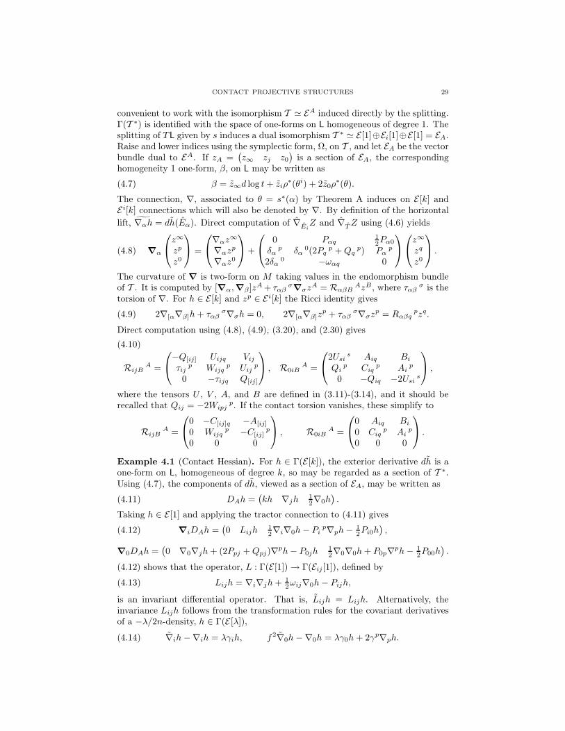
CONTACT PROJECTIVE STRUCTURES 29
convenient to work with the isomorphism T ≃ EA induced directly by the splitting.Γ(T ∗) is identified with the space of one-forms on L homogeneous of degree 1. Thesplitting of TL given by s induces a dual isomorphism T ∗ ≃ E [1]⊕Ei[1]⊕E [1] = EA.Raise and lower indices using the symplectic form, Ω, on T , and let EA be the vectorbundle dual to EA. If zA =
(z∞ zj z0
)is a section of EA, the corresponding
homogeneity 1 one-form, β, on L may be written as
(4.7) β = z∞d log t+ ziρ∗(θi) + 2z0ρ
∗(θ).
The connection, ∇, associated to θ = s∗(α) by Theorem A induces on E [k] andE i[k] connections which will also be denoted by ∇. By definition of the horizontal
lift, ∇αh = dh(Eα). Direct computation of ∇EiZ and ∇
TZ using (4.6) yields
(4.8) ∇α
z∞
zp
z0
=
∇αz
∞
∇αzp
∇αz0
+
0 Pαq12Pα0
δαp δα
0(2Pqp +Qq
p) Pαp
2δα0 −ωαq 0
z∞
zq
z0
.
The curvature of ∇ is two-form on M taking values in the endomorphism bundleof T . It is computed by [∇α,∇β ]zA + ταβ
σ∇σz
A = RαβBAzB, where ταβ
σ is thetorsion of ∇. For h ∈ E [k] and zp ∈ E i[k] the Ricci identity gives
2∇[α∇β]h+ ταβσ∇σh = 0, 2∇[α∇β]z
p + ταβσ∇σz
p = Rαβqpzq.(4.9)
Direct computation using (4.8), (4.9), (3.20), and (2.30) gives
RijBA =
−Q[ij] Uijq Vij
τijp Wijq
p Uijp
0 −τijq Q[ij]
, R0iB
A =
2Usis Aiq Bi
Qip Ciq
p Aip
0 −Qiq −2Usis
,
(4.10)
where the tensors U , V , A, and B are defined in (3.11)-(3.14), and it should berecalled that Qij = −2Wipj
p. If the contact torsion vanishes, these simplify to
RijBA =
0 −C[ij]q −A[ij]
0 Wijqp −C[ij]
p
0 0 0
, R0iB
A =
0 Aiq Bi
0 Ciqp Ai
p
0 0 0
.
Example 4.1 (Contact Hessian). For h ∈ Γ(E [k]), the exterior derivative dh is aone-form on L, homogeneous of degree k, so may be regarded as a section of T ∗.Using (4.7), the components of dh, viewed as a section of EA, may be written as
(4.11) DAh =(kh ∇jh
12∇0h
).
Taking h ∈ E [1] and applying the tractor connection to (4.11) gives
∇iDAh =(0 Lijh
12∇i∇0h− Pi
p∇ph− 12Pi0h
),(4.12)
∇0DAh =(0 ∇0∇jh+ (2Ppj +Qpj)∇
ph− P0jh12∇0∇0h+ P0p∇
ph− 12P00h
).
(4.12) shows that the operator, L : Γ(E [1]) → Γ(Eij [1]), defined by
(4.13) Lijh = ∇i∇jh+ 12ωij∇0h− Pijh,
is an invariant differential operator. That is, Lijh = Lijh. Alternatively, theinvariance Lijh follows from the transformation rules for the covariant derivativesof a −λ/2n-density, h ∈ Γ(E [λ]),
∇ih−∇ih = λγih, f2∇0h−∇0h = λγ0h+ 2γp∇ph.(4.14)
30 DANIEL J. F. FOX
Because the connection induced by ∇ on the canonical bundle is flat, the Ricciidentity implies 2∇[i∇j]h+ τij
α∇αh = 0. Tracing this gives ∇p∇ph = (1−n)∇0h,
so that the trace free part of ∇i∇jh− Pijh is Lijh. The skew part of Lijh, L[ij]his first order and vanishes when the contact torsion vanishes, so it makes sense tofocus attention on the contact Hessian, L(ij)h = ∇(i∇j)h− P(ij)h.
The projection TL → T induces a projection ⊗∗(TL) → ⊗∗(T ) on the full tensor
bundles. Denote by hB1...Bl
A1...Aka section of ⊗∗(T ). The tractor operator DIh
B1...Bl
A1...Ak
is defined by lifting the section hB1...Bl
A1...Akto an appropriately weighted tensor on L
to which the ambient connection is applied. The resulting tensor is projected downto give a section of ⊗∗(T ). This allows the iteration of the tractor D operator.
4.3. Contact Projective Structures Induced by Cartan Connections. Let(M,H) be a co-oriented contact manifold and π : G → M the corresponding Pprincipal bundle of filtered projective symplectic frames. The purpose of this sec-tion is to explain how a Cartan connection, η, on G, satisfying an appropriatecompatibility condition induces on M a contact projective structure. Each choiceof a square-root, ρ : L → M , determines a P principal bundle π : G → M and adouble covering Φ : G → G. The quotient G/P recovers L, and π : G → L is the
induced P principal bundle. A Cartan connection, η, on π : G →M pulls back viaΦ to a Cartan connection, also denoted η, on π : G → M , and will also be viewedas a Cartan connection on π : G → L. The group of principal bundle automor-phisms of G acts on the Cartan connections on G by pullback. A principal bundleautomorphism covering the identity on M will be called a change of gauge. Achange of gauge ψ : G → G has the form ψ(u) = u · p(u) where p : G → P is theP -equivariant function corresponding to a section, p, of the bundle G ×Ad(P ) P .
The pullback Cartan connection has the form ψ∗(η) = Ad(p−1)(η)+ p∗(ωP ), whereωP is the Maurer-Cartan form of P . The only case in which ψ∗(η) = η is whenp is a constant function and Ad(p) acts trivially on g. A choice of L determines aunique lift of a bundle automorphism of G to a bundle automorphism of G.
Call an η, on π : G →M , compatible with the co-oriented contact structure onM if η is regular; if the isomorphisms, η : TuG → g, are filtration-preserving; andif the induced isomorphisms, TuG/T
−1u G ≃ g/f−1, are orientation-preserving. It is
evident that compatibility is a gauge invariant condition. Compatibility impliesπ∗(η
−1(f−1)) = H and that the image of π∗(η−1(e0)) is consistent with the given
orientation on TM/H , and so, with regularity, that η induces the given co-orientedcontact distribution and its conformal symplectic structure. A (g, P ) Cartan con-nection η on π : G → M will be called compatible if it is induced by a compatible(g, P ) Cartan connection on π : G →M . Henceforth assume all η are compatible.
Viewing η as a Cartan connection on the P principal bundle, π : G → L, denoteby ∇η the affine connection induced on TL = G ×P V by (4.3). Call contact
non-slip a compatible Cartan connection for which ∇ηXX − X ∈ Γ(T 2L) for all
X ∈ Γ(T 1L). Using the definition of ∇η it may be checked that η is contact non-slip if and only if (∇η
Xα)(Y ) = 12Ω(X,Y ) for all X,Y ∈ Γ(T 1L). Likewise ∇ηX = δ
if and only if ∇ηα = 12Ω. If η is the Cartan connection defined from the ambient
connection, ∇, by (4.2), then ∇ηX = δ is condition 1 of Theorem B. Lemma 4.2shows that this condition should be interpreted as fixing a gauge.
Lemma 4.2. A given compatible (g, P ) Cartan connection on π : G → M isequivalent by a G0-valued change of gauge to a contact non-slip Cartan connection.
CONTACT PROJECTIVE STRUCTURES 31
Two gauge equivalent contact non-slip (g, P ) Cartan connections are related by aP+-valued change of gauge. Moreover, a given contact non-slip Cartan connectionis equivalent by a unique P+-valued change of gauge to a Cartan connection forwhich ∇ηX = δ; consequently, every compatible (g, P ) Cartan connection on π :G →M is gauge equivalent to a unique Cartan connection for which ∇ηX = δ.
Proof. For a compatible η let σ : U ⊂ L → G be a local section and set φ = σ∗(η).Under a change of gauge, ψ : G → G, as above, φ is replaced by Ad(b−1)(φ)+b∗(ωP ),where b = p σ : U → P . Write φ(X) = XQφQ with respect to an adaptedsymplectic frame, FI, on L, and represent φQ ∈ g by a matrix,
φQ =
AQ
∞ ∗ ∗AQ
p ∗ ∗AQ
0 −AQq −AQ∞
.
Because e∞ ∈ p, η(Xe∞) = e∞, and because π∗(Xe∞) = X, σ∗(X)−Xe∞ ∈ η−1(p),
so φ(X) · v∞ = e∞ · v∞ = v∞. This shows A∞∞ = 1, A∞
p = 0, and A∞0 = 0.
From the compatibility of η there follows φ(X) ∈ f−1 if and only if X ∈ T 1L, andthis implies Ai
0 = 0. Regularity, Ai0 = 0, and A∞
0 = 0, imply that AipAj
qωpq =Ω(φ(Fi) · v∞, φ(Fj) · v∞) = 1
2 Ω([φ(Fi), φ(Fj)] · v∞, v∞) = −α(φ([Fi, Fj ]) · v∞) =
A00ωij . Compatibility implies A0
0 = c2 > 0. Let Bqp be the unique symplectic
matrix such that cBsjAi
s = δij . The change of gauge given by b : L → G0
defined by b−1 = exp(c−1v∞ ⊗ v∞ + Bpqvq ⊗ vp + cv0 ⊗ v0) produces a contact
non-slip connection. As the image in P/P of b is non-trivial, the contribution ofb∗(ωP ) under this change of gauge is non-trivial, effecting the components AI
∞.
Because the adjoint action of P on P/P is trivial, b∗(ωP )(X) ∈ p, and the identityA∞
∞ = 1 persists. Thus every compatible Cartan connection is gauge equivalentto a contact non-slip Cartan connection. Now suppose given a contact non-slipCartan connection and set γp = A0
p and γ0 = A0∞ − γsA0
s. For b : U → P+
defined by b = exp(γpv∞ ⊗ vp + γpvp ⊗ v0 + γ0v∞ ⊗ v0), Ad(b−1)(φ) + b∗(ωP )satisfies ∇ηX = δ. Similar easy computations show that gauge equivalent contactnon-slip Cartan connections must be related by a change of gauge of the formb = exp(γpv∞ ⊗ vp + γpvp ⊗ v0 + γ0v∞ ⊗ v0) ∈ P+. The same computation showsthat a change of gauge preserving the condition ∇ηX = δ must be trivial.
Recall Cartan’s notion of development as described in section 4 of chapter 5 of[17]. If γ : [a, b] = I → G is any lift of γ : [a, b] = I → M , there is a uniquec : I → G such that c∗(ωG) = γ∗(η) and c(a) = e ∈ G, where ωG is the Maurer-Cartan form of G. While the curve c depends on the choice of lift, its projectionΨ c : I → G/P is well-defined up to the action of P on G/P , and is called thedevelopment of γ. (Note that in the proof of Proposition 4.13 in [17] Lemma4.12 of [17] is misapplied to incorrectly conclude that the projection into G/P ofc does not depend on the choice of lift; the issue is the choice of a basepoint).Two parameterized curves with the same path develop onto curves with the samepath, so it makes sense to say that the development of a path on M is a memberof a P -invariant family of paths in P(V), e.g. it makes sense to say that a pathdevelops onto a line. Since the family of contact lines (resp. all lines) in G/P isinvariant under the action of P on G/P , the statement that a path in M developsonto a contact line (resp. line) in G/P is independent also of the choice of Cartanconnection representing the isomorphism class of η. If η is the Cartan connection
32 DANIEL J. F. FOX
built from the ambient connection, direct computation as in the proof of Proposition8.3.5 of [17] and using the explicit description of η implicit in (4.8) shows that thepaths of η which develop onto isotropic lines are exactly the contact geodesics andthe paths which develop onto lines are exactly the geodesics of the subordinateprojective connection of Theorem 3.2. Consequently, for an arbitrary compatible η,it makes sense to define the induced contact projective structure to comprise thosecontact paths in M which develop onto contact lines in G/P . There are in generalmany Cartan connections on G inducing a given contact projective structure.
A compatible η induces on the G principal bundle, G ×P G→ L, the G principalconnection, µ, induced by the connection µu,b = Ad(b−1)(π∗
G(η)) + π∗G(ωG) on
G ×G, where πG and πG are the projections onto the factors of G ×G, and ωG isthe Maurer-Cartan form of G. G ×P G is naturally identified with the symplecticframe bundle of TL and the induced ∇η is just the affine connection on L inducedby µ. Moreover, if c : I → G is associated as above to the lift γ of γ : I →M , thenγ(t) = [γ(t), c−1(t)] is a horizontal curve, γ : I → G ×P G, covering γ. Using this itmay be checked that the paths in L which develop via η onto lines in V are exactlythe unparameterized geodesics of ∇η. Evidently these are the horizontal lifts of thepaths in M which develop onto lines in P(V).
Using (4.3), it is straightforward to show that, for compatible η, ∇ηΩ = 0 and∇η
XX = X. Let τη and Rη be the torsion and curvature of ∇η. Using that η is
contact non-slip and ∇ηXX = X, and computing directly the curvature shows that,
for all X,Y ∈ Γ(T 1L), τη(X,Y ) − Rη(X,Y )X ∈ T 2L. The curvature function,κ(h1, h2), of η vanishes whenever either h1 or h2 is in p, so, by (4.4), Rη(X, X)X =κ(η(X), η(X)) · v∞ = 0, and consequently τη(X, X) ∈ T 2L for all X ∈ Γ(T 1L).Next the induced contact projective structure is described more analytically. Fora section, s : M → L, let θ = s∗(α) and define an affine connection, ∇, on M by
∇XY = ρ∗(∇η
XY ). For a contact non-slip η, the restrictions to T 1L × T 1L of ∇ηα
and 12Ω agree, and this implies that Sym∇θ vanishes when restricted to H×H . By
Lemma 2.1, the geodesics of ∇ determine a contact projective structure. Becauseη is contact non-slip,
∇ηXY − Y = (∇η
YX − Y ) + τη(X, Y ) ∈ T 2
L for Y ∈ Γ(H).(4.15)
In particular, ρ∗(∇ηXY ) = Y . If s = fs and direct computation using (4.15) shows
that the connection, ∇, induced on M by s determines the same contact projectivestructure as does ∇. Moreover it is straightforward to check, as in the proof ofTheorem 3.2, that the contact geodesics of the induced contact projective structureare the images in M of the paths of the geodesics of ∇η transverse to the verticaland tangent to kerα. By the remarks above the geodesics of ∇η tangent to kerαdevelop onto contact lines in V, and hence their images in M develop onto contactlines in P(V), so the induced contact projective structure is the same as the contactprojective structure defined using development. To show via the tractor connectionthat gauge equivalent contact non-slip Cartan connections, η and µ, induce thesame contact projective structure, choose s : M → L and compute the differencetensor, Λ, of the connections ρ∗(∇µ
XY ) and ρ∗(∇η
XY ). Computing directly using
(4.3) and Lemma 4.2 shows that Λijk = γkωij + γjδi
k and Λij0 = ωij . By Lemma
2.2, the induced contact projective structures are the same.
CONTACT PROJECTIVE STRUCTURES 33
4.4. Algebraic Characterization of Curvature of Canonical Cartan Con-
nection. The purpose of this section is to reformulate conditions 4 and 5 of The-orem B as algebraic conditions on the curvature function of the associated Cartanconnection, and to prove Theorem C.
There is a co-boundary operator, ∂ :∧k
((g−)∗) ⊗ g →∧k+1
((g−)∗) ⊗ g, (see[27]), defined when k = 2 by
∂φ(x1, x2, x3) = Cycle [x1 · φ(x2, x3) − φ([x1, x2], x3)] .
Any invariant, symmetric bilinear form, B, on g is a constant multiple of the Killingform, and soB gives an identification (p+)∗ ≃ g−. Let eα be a basis for g− and let eα
be the B-dual basis for p+. The formal adjoint with respect to B of the co-boundary∂ is a boundary ∂∗ :
∧2(g∗−) ⊗ g → g∗− ⊗ g defined by B(∂∗ψ, φ) = −B(ψ, ∂φ) for
ψ ∈ ∂∗ :∧2
(g∗−) ⊗ g and φ ∈ g∗− ⊗ g. Via the linear isomorphism, g/p ≃ g−,induced by B, the adjoint action makes g− a P -module; it can be checked that ∂∗
is P -equivariant. Recall that a Cartan connection is normal if ∂∗κ = 0.Because the tractor connection, ∇ = ∇η, is the induced connection on the
associated bundle, G ×P V, its curvature, R, may be computed from the curvatureof η, as in (4.4). By (4.10), κ−2 = 0; in particular, η is regular. The isomorphismη : TuG → g induces an adjoint map ηt : g∗ → T ∗
uG. Because kerB(e0,−) = f−1,and Ad(P )(g−2) = g−2, the image under π∗ of the horizontal subbundle of T ∗Gspanned by ηt(B(e0,−)) is the annihilator of H . Let eI and vI be as in Section 2.4,and define a frame on M by Ei = π∗(η
−1(ei)) and T = π∗(η−1(2e0)). Choose θ such
that θ(T ) = 1 and θ annihilates H . Because π∗(θ) is a multiple of ηt(B(e0,−))and κ−2 = 0, dθ(Eα, Eβ) = 2ωαβ, so that θ is a contact one-form with Reebfield T . Choose also a θ-adapted coframe dual to the given frame. By (4.4) thecomponents, κ(ei, ej), of the curvature function are identified with the components,Rij , of the curvature of the tractor connection, and 2κ(e0, ei) = R0i. ChooseB so that with respect to the standard representation, ρ : Sp(n,R) → GL(V),B(x, y) = 1
2 tr (ρ(x)ρ(y)). With respect to the basis vI ⊗ vJ of g ⊂ V ⊗ V∗,
ei = vi ⊗ v∞ − ωiqv0 ⊗ vq, e0 = v0 ⊗ v∞, e∞ = v∞ ⊗ v∞ − v0 ⊗ v0,
ei = v∞ ⊗ vi + ωpivp ⊗ v0, e0 = 2v∞ ⊗ v0.
Proposition 4.1. The Cartan connection, η, is normal if and only if the underlyingcontact projective structure has vanishing contact torsion.
Proof. In general ∂∗κ(x) = [eα, κ(eα, x)] −12κ(eα, [e
α, x]−), which gives
∂∗κ(ej) = [e0, κ(e0, ej)] + [ei, κ(ei, ej)], ∂∗κ(e0) = [ei, κ(ei, e0)] −12κ(ei, [e
i, e0]−).
Direct computation of ∂∗κ(ej) using (3.20), and direct computation of ∂∗κ(e0)using [ei, e0] = −ωijej , (2.30), (2.31), and (3.20) give
∂∗κ(ej) =
0 −Qjq + 12Qqj −2Usj
s
0 τjp
q + τjqp −Qj
p + 12Q
pj
0 0 0
∂∗κ(e0) =
0 Usqs + 1
2Uss
q12Vs
s
0 12 (Qp
q +Qqp) Us
ps + 12Us
sp
0 0 0
If ∂∗κ(ej) = 0, then τj(pq) = 0, from which follows 0 = 2τi(jk) − 2τj(ik) = 3τijk,so that ∂∗κ = 0 implies the contact torsion vanishes. On the other hand, τijk = 0
34 DANIEL J. F. FOX
implies Qij = 0 and P[αβ] = 0, and, by (3.20), it implies also Vss = 0 and Us
ps = 0.(3.5), (3.20), and (3.17) show Us
sq + 2Usq
s = −2∇pPpq + (2n − 1)P0q = ∇pQpq,so that Us
sq + 2Usq
s vanishes also. Thus τijk = 0 implies ∂∗κ(eα) = 0.
The goal of the remainder of this subsection is to describe the P submodule,K ⊂ C2(g−, g), appearing in the statement of Theorem C. Given a compatible(g, P )-Cartan connection on the principal P -bundle G → M , let ∇ = ∇η be theinduced covariant differentiation on the associated tractor bundle T = G ×P V.Let Rαβ be the components with respect to Eα of the g-valued curvature two-formof ∇, so Rij = κ(ei, ej) and R0i = 2κ(e0, ei). Because the η constructed fromthe ambient connection always satisfies κ−2 = 0, it will be assumed that κ−2 = 0,which implies that R has the form
RijAB =
aij cijq eij
bijp dijq
p cijp
0 −bijq −aij
, R0iA
B = 2
ai ciq ei
bip diq
p cip
0 −biq −ai
,(4.16)
where dij[qp] = 0 and di[qp] = 0 are forced by the requirement that these matricesare in g. Rewritten in terms of κ, the Bianchi identity, dK = [K, η], becomes
(4.17) ∂κ(h1, h2, h3) + Cycle[κ(κ−(h1, h2), h3) + Lη−1(h1)(κ(h2, h3))
]= 0.
In (4.17), Lη−1(h1)(κ(h2, h3)) is the Lie derivative of the function κ(h2, h3) : G → g.Because κ−2 = 0, (4.17) implies (∂κ)−2(eα, eβ , eγ) = 0, giving
Cycle ([ei, κ−1(ej , ek)] + ωijκ−2(e0, ek)) = 0,(4.18)
[e0, κ0(ei, ej)] + [ei, κ−1(ej , e0)] + [ej, κ−1(e0, ei)] = 0.(4.19)
As [ek, κ−1(ei, ej)] = bijke0, (4.18) shows b[ijk] = 0. Direct computation using
(4.19) gives aij = −2b[ij] so that RαβBA has the form
RijAB =
−2b[ij] cijq eij
bijp dijq
p cijp
0 −bijq 2b[ij]
, R0iA
B = 2
ai ciq ei
bip diq
p cip
0 −biq −ai
.(4.20)
Because of the curvature and torsion normalizations of Theorem B, the curvatureof the Cartan connection, η, built from the ambient connection has the form (4.10)and satisfies additionally,
τ[ijk] = 0, τpip = 0 = τp
pi, P[ij] = −2Q[ij], Qp
p = 0,
Wpp
ij = 0, Wipj
p = − 12Qij , Upi
p = P[0i], Cppi = 0, Ap
p = 0,
which motivate Definition 4.1. In Definition 4.1 and Lemma 4.3, κ should beunderstood as an element of the P -module C2(g−, g).
Definition 4.1. The subspace K ⊂ C2(g−, g) comprises κ of the form (4.20), i.e.
κ−2 = 0, aij = −b[ij], b[ijk] = 0,(4.21)
and satisfying the following additional requirements
bpip = 0, bp
pi = 0, bp
p = 0,(4.22)
cpip = ai, dipj
p = −bij , dppi = 0, dp
pi
j = 0, cpp = 0.(4.23)
Lemma 4.3. K is a P -submodule of C2(g−, g).
CONTACT PROJECTIVE STRUCTURES 35
Proof. For b ∈ P , let eα = ad(b)(eα), let κ = b · κ, and write καβ = κ(eα, eβ) =Ad(b−1)(κ(eα, eβ)). The adjoint action of P on g−2 is trivial which suffices to showthe P -invariance of the condition κ−2 = 0. Assuming (4.21), direct computation
∂∗κ(ej) =
bij
i −2bjq − djiqi + bqj −2aj + 2cij
i
0 bjp
q + bjqp −2bj
p + bp j − djipi
0 0 −biji
,(4.24)
∂∗κ(e0) =
−bll aq − dsq
s + 12cs
sq
12es
s − 2css
12bs
sp bqp + bp q + 1
2dss
qp −ds
sp + ap + 12cs
sp
0 − 12bs
sq bs
s
.(4.25)
From these it is apparent that in the presence of (4.21) the requirement that∂∗κ ∈ C1(g−, p) is equivalent to (4.22). Representing b ∈ P+ by exp(γqe
q + 12γ0e
0)and computing directly gives ei = ei and e0 = e0 + γpep, from which followκij = ad(b−1)(κij), and κ0i = ad(b−1)(κ0i + γsκsi), for b ∈ P+. Further directcomputation gives the components of καβ − καβ ,
b[ij] − b[ij] = − 12γ
pbijp,(4.26)
bijp − bij
p = 0,(4.27)
cijk − cijk = −2γkb[ij] + γ0bijk + γkγpbijp + γpdijkp,(4.28)
dijkl − dijk
l = bijlγk + γlbijk,(4.29)
eij − eij = −4γ0b[ij] − 2γ0γpbijp + 2γpcijp − γpγqdijpq ,(4.30)
ai − ai = 2γpbip − γpbpi + γqγpbqip,(4.31)
bij − bij = γpbpij ,(4.32)
dijk − dij
k = bikγj + γkbij + γp
(dpij
k + γjbpik + γkbpij
),(4.33)
cij − cij = aiγj + γ0bij(4.34)
+ γp (γjbip + dijp + cpij − γjγqbpiq + γqdpijq) ,
ei − ei = 2γ0ai + γp (2cip − 2γ0bip + epi)(4.35)
− γpγq (dipq + 2γ0bpiq − 2cpiq + γrdpiqr) .
Represent b ∈ G0 by b = exp(f−1v∞ ⊗ v∞ + Fqpvp ⊗ vq + fv0 ⊗ v0), where
FipFj
qωpq = ωij . For such b direct computation gives ei = fFipep, and e0 = f2e0,
from which follow
κij = ad(b−1)(f2FipFj
qκpq), κ0i = ad(b−1)(f3Fipκ0p), for b ∈ G0.
Defining Gpi by Fi
pGpj = δi
j , further direct computation gives
κij = f2FiuFj
v
auv fcuvpFqp f2euv
f−1Gqpbuv
q duvrsGs
pFqr fcuvsF
ps
0 −f−1Gsqbuvs −auv
,(4.36)
κ0i = f3Fiu
au fcupFqp f2eu
f−1Gqpbu
q GspFq
rdurs fGq
pcuq
0 −f−1bupFqp −au
.(4.37)
(4.26), (4.32), (4.27), (4.36), and (4.37) show directly the P -invariance of the condi-tions aij = −b[ij], b[ijk] = 0, and (4.22). The P -invariance of the conditions (4.23)
36 DANIEL J. F. FOX
follows from (4.28), (4.29), (4.31), (4.32), (4.33), (4.34), (4.36), and (4.37) by directcomputation.
It is desirable to find a conceptual description of K that makes clear its P -invariance. The conditions in (4.21) other than κ−2 = 0 are purely algebraic con-sequences of the Bianchi identities, (4.18) and (4.19), and so must be P -invariant.As ∂∗ is P -equivariant and p is invariant under the adjoint action of P on g, thecondition that ∂∗κ take values in p is P -invariant, and so the equivalent conditions(4.22) are P -invariant as well. The formulation of the remaining conditions is adhoc and so demonstration of their P -invariance requires explicit computations.
Proof of Theorem C. The construction from the ambient connection of the Cartanconnection demonstrates the existence of a regular (g, P ) Cartan connection induc-ing the given contact projective structure, having curvature in K, and satisfying∇ηX = δ. Now let η be a compatible (g, P ) Cartan connection with curvaturein K and inducing the given contact projective structure. By Lemma 4.2, η isgauge equivalent to a Cartan connection for which the associated covariant differ-entiation, ∇η, on TL = G ×P V, satisfies ∇ηX = δ. Let Rη and τη denote thecurvature and torsion of ∇η, and recall that ∇ηΩ = 0. From ∇ηX = δ there followsRη(X, X)X = τη(X, X), and Rη(X, X)X = 0 by (4.4), so that τη(X,−) = 0. Thisshows that ∇η satisfies conditions 1-3 of Theorem B.
Because kerB(e0,−) = f−1, the one-form ψ0 = ηt(B(e0,−)) is horizontal and
annihilates η−1(f−1). Because Ad(b)(e0) = e0 for all b ∈ P , though not for all
b ∈ P , ψ0 is P -invariant, though it is not P -invariant, and hence ψ0 is the pullbackof some one-form on L which, by compatibility, annihilates kerα. Because ∇ηX = δ,the frame defined in TL by FI = π∗(η
−1(eI)), is an adapted symplectic frame, andfrom this there follows π∗(α) = 1
2ψ0. By (4.4), Rη
PQRSeS = κ(eP , eQ) · eR. It
was already observed that Rη∞QR
S = 0 and RηPQ∞
S = τηPQ
S . Because ∇ηΩ = 0,
the Ricci identity gives Rη
PQ(AB) = RηPQAB. Consequently, Rη
ABC0 = −Rη
ABC∞ =
−RηAB∞C = −τη
ABC . By the preceeding, RηIJ = Rη
IQJQ = Rη
IqJq − τη
I0J . Nowexplicit computations using the conditions defining K show 4 and 5, so that ∇η
satisfies all the conditions of Theorem B. The uniqueness statement in Theorem Bshows ∇η must be the ambient connection of the given contact projective structure,from which there follow the identifications
bijk = τijk, cijk = Uijk, dijkl = Wijkl , eij = Vij ,(4.38)
2bij = Qij , 2cij = Aij , 2dijk = Cijk, 2ei = Bi.(4.39)
The identification τijk = bijk and Proposition 4.1 show that η is normal if and onlythere vanishes the contact torsion of the underlying contact projective structure.Direct computation shows that a change of gauge preserving condition 1 must betrivial, so that this condition singles out the ambient connection as a distinguishedrepresentative of the given isomorphism class of Cartan connections.
Remark 4.1. By (4.38) and (4.39), the application to the Cartan connection con-structed from the ambient connection of the transformation formulae in (4.26)-(4.35) gives the rules for the transformations of the components of the curvatureof the ambient connection under change of scale. For example, (4.27) shows theinvariance of the contact torsion, (4.29) recovers (2.38), and (4.33) recovers (2.39).
CONTACT PROJECTIVE STRUCTURES 37
5. Applications
5.1. Lifting Projective Structures on Integral Symplectic Manifolds. Anintegral symplectic manifold admits a canonical contactification, and projectivestructures on the symplectic manifold can be lifted to contact projective structureson the contactification. This construction provides many examples of contact pro-jective structures. It is necessary to take the slightly unusual perspective of allowingthe affine connections representing a projective structure to have torsion.
Proposition 5.1. Given a projective structure on the symplectic manifold (N,ω),there exists a unique affine connection, ∇, representing the projective structure,having torsion, τ , and such that
1. ∇ω = 0.
2. The trace of the torsion of ∇ vanishes.
Proof. Raise and lower indices with ω. Let ∇ be a connection with torsion, τ ,representing the given projective structure, and define ∇ by letting its differencetensor with ∇ be Λijk = −∇kωij −
32τ[ijk]. As Λ(ij)k = 0, ∇ represents the given
projective structure. (2.4) and (2.5) show ∇kωij = 0. Consequently ∇ may beassumed to make parallel ω. If ∇ is another representative of the given projectivestructure satisfying Condition 1, there must be a one-form, γ, so that the differencetensor, Λij
k, of ∇ and ∇, satisfies Λ(ij)k = 12n+1 (ωikγj + ωjkγi), and Λk[ij] = 0.
Because a three tensor skew in two indices and symmetric in two indices mustvanish, the most general possible choice for Λijk is Λijk = 2
2n+1 (ωijγk + ωikγj).Tracing the difference of the torsion tensors shows that the unique choice of γ sothat 2 holds also is γi = 1
2τipp.
On a symplectic manifold, (N,ω), such that ω represents an integral cohomologyclass [ω] ∈ H2(N,Z), there is a principal S1-bundle π : M → N with connectionone-form, θ, such that the curvature dθ = π∗ω. The kernel of θ is a contactstructure on M and the infinitesimal generator, T , of the principal S1 action isthe Reeb vector field of θ. The collection of all horizontal lifts of the paths in aprojective structure on N determines on M a contact path geometry, which willnow be shown to be a contact projective structure. Fix ∇ representing the givenprojective structure and making ω parallel. Define on M a connection, ∇, by
∇XY = ∇XY , ∇
XT = 0, ∇T X = LT X,
where X is the horizontal lift determined by θ of the vector field X on N . It isstraightforward to check that ∇θ = 0, ∇dθ = 0, and i(T )τ = 0. Moreover, if ∇ isthe unique representative given by Proposition 5.1, then the trace of the torsion of∇ vanishes, so that ∇ is the unique connection associated to θ by Theorem A.
5.2. Pseudo-Hermitian Beltrami Theorem. Recall the classical
Theorem 5.1 (Beltrami Theorem). The projective structure determined by thegeodesics of a Riemannian metric is flat if and only if the Riemannian metric hasconstant sectional curvatures.
The proof, which is an exercise in using the Bianchi identities, is in [9]. Next thereis proved an analogous theorem for pseudo-hermitian manifolds.
38 DANIEL J. F. FOX
A pseudo-hermitian structure is a contact manifold equipped with a distin-guished contact one-form, θ, and an almost complex structure, J , on H . HereJ : H → H is a real automorphism such that Ji
pJpj = −δi
j and assumed tosatisfy the compatibility condition
(5.1) [J(X), Y ] + [X, J(Y )] ∈ Γ(H) ∀X,Y ∈ Γ(H).
If in addition J satisfies
(5.2) [J(X), J(Y )] − [X,Y ] = J([J(X), Y ] + [X, J(Y )]) ∀X,Y ∈ Γ(H)
then the pseudo-hermitian structure is said to be integrable. By assumption (5.1),the inner product defined on H by gij = −Jij is symmetric, and because dθ is non-degenerate on H , g is non-degenerate on H . The almost complex structure Jdetermines an (n− 1)-dimensional complex subbundle of the complexified tangentbundle, T1,0 ⊂ CTM , comprising vector fields of the form X+iJ(X) for X ∈ Γ(H).Define the Levi form, L(U, V ) = −iω(U, V ) for U, V ∈ Γ(T1,0).
In [19] and [20], Tanaka constructed a canonical affine connection associated toa pseudo-hermitian structure. In the integrable case his construction specializes asin the following theorem, the statement of which is taken from [21].
Theorem 5.2 (N. Tanaka). On an integrable pseudo-hermitian manifold thereexists a unique affine connection, ∇, the pseudo-hermitian connection, havingtorsion τ and satisfying:
1. ∇θ = 0.
2. ∇dθ = 0.
3. τijγ = ωijδ0
γ .
4. JipAp
j = −AipJp
j where Aαβ = τ0α
β is the pseudo-hermitian torsion.
By definition A0β = 0; by Condition 2, Aα
0 = 0; and by (2.7), A[ij] = 0. By
Condition 1, Lemma 2.1 implies that the geodesics of ∇ induce a contact projectivestructure. Define a connection, ∇, by ∇XY − ∇XY = Λ(X,Y ), where Λαβ
γ =−δα
0Aβγ . Because Λ(ij)
γ = 0, ∇ admits the same full set of contact geodesics
as does ∇. Moreover, ∇ is the representative associated to θ by Theorem A. That∇θ = 0 and ∇ω = 0 follow by direct computation using (2.4). The torsions arerelated by ταβ
γ − ταβγ = 2δ[α
0Aβ]γ , so that τ0β
γ = Aβγ −Aβ
γ = 0, and τijk = 0
(so that τipp = 0). This shows ∇ satisfies the conditions of Theorem A and proves:
Proposition 5.2. An integrable pseudo-hermitian structure induces a contact pro-jective structure with vanishing contact torsion.
Note that, while ∇kJij = 0, ∇0Ji
j = 2AipJp
j . Let Rαβγσ denote the curvature
of ∇. Lemma 2.32 shows that
Rijkl −Rijk
l = ωijAk,l , R0ij
k −R0ijk = −∇iAj
k = −∇iAjk.(5.3)
Define a quadratic form on T1,0 by Q(Z) = L(R(Z, Z)Z,Z) for Z ∈ Γ(T1,0). ForZ ∈ Γ(T1,0), Webster, [24], defined by Q(Z) = K(Z)L(Z,Z)2 the holomorphic
sectional curvature, K(Z), of the subspace spanned by Z and Z. The pseudo-hermitian structure has constant sectional curvature κ if there is a constantκ so that K(Z) = κ for all Z ∈ Γ(T1,0). The pseudo-hermitian connection is saidto have transverse symmetry if Aij = 0. The following theorem is the desiredpseudo-hermitian analogue of the Beltrami theorem.
CONTACT PROJECTIVE STRUCTURES 39
Theorem 5.3. The contact projective structure induced by an integrable pseudo-hermitian structure having transverse symmetry is flat if and only if the pseudo-hermitian structure has constant sectional curvatures.
Proof. Extend Jij to Jαβ by setting Jα0 = 0 = J0β . Because Aij = 0, the preceed-ing discussion shows that the pseudo-hermitian connection, ∇ = ∇, is the represen-tative associated to θ by Theorem A of the contact projective structure induced bythe given pseudo-hermitian structure. By Proposition 5.2 the induced contact pro-jective structure has vanishing contact torsion and so, by the first Bianchi identity,(2.14), R[αβγ]
δ = 0. By the Ricci identity and ∇J = 0,
(5.4) RαβγpJpδ = −Rαβδ
pJpγ ,
so that the tensor RαβγqJqδ has the same symmetries as does the curvature of a
Levi-Civita connection, and a standard argument implies that
(5.5) RαβγqJqδ = Rγδα
qJqβ .
By the non-degeneracy of Jij , R0ijqJqk = Rjk0
qJqi = 0 implies R0ijk = 0. Sinceτijk = 0 and Wijkl = 0, expanding (5.4) gives
0 =RikJjl −RjkJil + ωjkRipJpl − ωikRj
pJpl − 2ωijRkpJpl+(5.6)
RilJjk −RjlJik + ωjlRipJpk − ωilRj
pJpk − 2ωijRlpJpk.
Set R = RpqJpq. Tracing (5.4) in ij and using (2.15) gives Ji
qRqpJpk = −Rik, so
that tracing (5.6) with Jjl gives
2(n− 1)Rij = JijR,(5.7)
4n(n− 1)Rijkl = R(ωjlJik − ωilJjk + ωjkJil − ωikJjl − 2ωijJkl).(5.8)
When 2n − 1 = 3 the hypothesis is Cijk = 0, and when 2n − 1 ≥ 5 Lemma 2.7shows that Wijkl = 0 implies Cijk = 0. So C(ijk) = 0, which, by 0 = R0ijk , (2.29),
and (5.7), implies 0 = 12n(n−1)J(ij∇k)R. Tracing this with J ij gives ∇kR = 0. By
the traced second Bianchi identity, (2.21), and the vanishing of R0ijk, ∇0Rij =−∇pR0ij
p = 0, so, by (5.7), 0 = Jij∇0R, and tracing this shows ∇0R = 0. ThusR is a constant function. Using (5.4) in (5.8) gives n(1 − n)RipklJj
pxixjxkxl =Rgijgklx
ixjxkxl, which implies n(n− 1)Q(Z) = RL(Z,Z)2 for all Z ∈ Γ(T1,0), sothat the pseudo-hermitian structure has constant sectional curvatures.
Assume given the contact projective structure induced by a pseudo-hermitianstructure with transverse symmetry and constant sectional curvatures. Using (5.5)and the other symmetries of Rijkl shows RpqklJi
pJjq = Rijkl . Polarizing the
equality of quartic forms n(1−n)RipklJjpxixjxkxl = Rgijgklx
ixjxkxl given by theassumption of constant sectional curvature gives Rp(ijkJl)
p = cg(ijgkl), and using(5.5), RpqklJi
pJjq = Rijkl , and relabeling gives
(5.9) Rljki −Rjkli +RplqiJjqJk
p = c(ωjigkl + ωjlgik + ωjkgil).
Tracing (5.9) in ij and usingRpqklJipJj
q = Rijkl and (5.5) gives (5.8), for a suitableconstant, R. This implies (5.7) and hence Wijkl = 0, so that if the dimension is atleast 5, the contact projective structure is flat. In three dimensions, R0ijk = 0, soCijk = 1
n∇(iRjk), which vanishes by (5.7).
Example 5.1. In [15], V. Matveev studies the space of Riemannian metrics projec-tively equivalent to a given Riemannian metric. An analogous problem is to describethe space of pseudo-hermitian structures determining the same contact projective
40 DANIEL J. F. FOX
structure. Two pseudo-hermitian structures are homothetic if their contact one-forms differ by a constant. Two pseudo-hermitian structures represent the sameCR structure if their contact one-forms differ by a non-vanishing scale factor. It iseasy to prove that conformally equivalent Riemannian metrics determine the sameprojective structure if and only if they are homothetic. Similarly, using (2.8) andthe analogous formula for the transformation of the pseudo-hermitian connectionunder a change of scale, it may be shown that, if the dimension is at least five, twointegrable pseudo-hermitian structures representing the same CR structure gener-ate the same contact projective structure if and only if they are homothetic. Theidea for the following example of non-homothetic, contact projectively equivalentpseudo-hermitian structures comes from Matveev’s description, [15], of Beltrami’sexample of projectively equivalent non-homothetic Riemannian metrics. Any linearconformal symplectic automorphism, A, of (R2n,Ω), determines the contactomor-phism, x→ ψ(x) = |Ax|−1Ax, of S2n−1. As A preserves linear isotropic subspaces,ψ preserves the intersections with S2n−1 of isotropic subspaces. These intersectionsare equatorial spheres each of which is everywhere tangent to the contact hyper-plane. In particular, ψ maps contact lines on S2n−1 to contact lines, so ψ is an au-tomorphism of the standard flat contact projective structure on S2n−1. EquippingCn with the standard Hermitian form the imaginary part of which is Ω induceson the unit sphere, S2n−1, the standard pseudo-hermitian structure. Because ψis a contactomorphism, the standard pseudo-hermitian structure on S2n−1 may bepulled back via ψ. As ψ preserves contact circles, the contact geodesics of the pulledback pseudo-hermitian structure are necessarily the same as those of the standardpseudo-hermitian structure. ψ is a homothety of the standard pseudo-hermitianstructure if and only if it agrees with the restriction to S2n−1 of a scalar multipleof a unitary linear transformation, and it is easily checked that this happens if andonly if A is a scalar multiple of a unitary transformation. Consequently, if A isnot a constant multiple of a unitary transformation, then these pseudo-hermitianstructures are not homothetic, though they induce equivalent contact projectivestructures.
References
[1] T. N. Bailey, M. G. Eastwood, and A. R. Gover, Thomas’s structure bundle for conformal,
projective and related structures, Rocky Mountain J. Math. 24 (1994), no. 4, 1191–1217.
[2] A. Cap and A. R. Gover, Standard tractors and the conformal ambient metric construction,Ann. Global Anal. Geom. 24 (2003), no. 3, 231–259.
[3] , Tractor calculi for parabolic geometries, Trans. Amer. Math. Soc. 354 (2002), no. 4,1511–1548.
[4] A. Cap and H. Schichl, Parabolic geometries and canonical Cartan connections, HokkaidoMath. J. 29 (2000), no. 3, 453–505.
[5] A. Cap and J. Slovak, Weyl structures for parabolic geometries, Math. Scand. 93 (2003),no. 1, 53–90.
[6] A. Cap, J. Slovak, and V. Soucek, Bernstein-Gelfand-Gelfand sequences, Ann. of Math. (2)154 (2001), no. 1, 97–113.
[7] E. Cartan, Sur les varietes a connexion projective, Bull. Soc. Math. France 52 (1924), 205–241.
[8] S.-S. Chern, The geometry of the differential equation y′′′ = F (x, y, y′, y′′), Sci. Rep. Nat.Tsing Hua Univ. (A) 4 (1940), 97–111.
[9] S. S. Chern and P. Griffiths, Abel’s theorem and webs, Jahresber. Deutsch. Math.-Verein. 80(1978), no. 1-2, 13–110.

CONTACT PROJECTIVE STRUCTURES 41
[10] W. Fulton and J. Harris, Representation theory, Graduate Texts in Mathematics, vol. 129,Springer-Verlag, New York, 1991.
[11] A. R. Gover, Invariants and calculus for projective geometries, Math. Ann. 306 (1996), no. 3,513–538.
[12] C. R. Graham, Invariant theory of parabolic geometries, Complex geometry (Osaka, 1990),Dekker, New York, 1993, pp. 53–66.
[13] J. Harrison, Some problems in the invariant theory of parabolic geometries, Ph.D. thesis,University of Edinburgh, 1995, pp. 1–120.
[14] S. Kobayashi and T. Nagano, On projective connections, J. Math. Mech. 13 (1964), 215–235.[15] V. S. Matveev, Hyperbolic manifolds are geodesically rigid, Invent. Math. 151 (2003), no. 3,
579–609.[16] T. Morimoto, Geometric structures on filtered manifolds, Hokkaido Math. J. 22 (1993), no. 3,
263–347.[17] R. W. Sharpe, Differential geometry, Graduate Texts in Mathematics, vol. 166, Springer-
Verlag, New York, 1997.[18] J. Slovak, Parabolic geometries, IGA Preprint 97/11 (1997), 1–70, available at http://
www.maths.adelaide.edu.au/Pure/iga/preprints.html.[19] N. Tanaka, On the equivalence problems associated with a certain class of homogeneous
spaces, J. Math. Soc. Japan 17 (1965), 103–139.
[20] , A differential geometric study on strongly pseudo-convex manifolds, KinokuniyaBook-Store Co. Ltd., Tokyo, 1975, Lectures in Mathematics, Department of Mathematics,Kyoto University, No. 9.
[21] , On non-degenerate real hypersurfaces, graded Lie algebras and Cartan connections,Japan. J. Math. (N.S.) 2 (1976), no. 1, 131–190.
[22] , On the equivalence problems associated with simple graded Lie algebras, HokkaidoMath. J. 8 (1979), no. 1, 23–84.
[23] T. Y. Thomas, The differential invariants of generalized spaces, Chelsea Publishing Company,New York, N.Y., 1934.
[24] S. M. Webster, Pseudo-Hermitian structures on a real hypersurface, J. Differential Geom. 13(1978), no. 1, 25–41.
[25] H. Weyl, Zur Infinitesimalgeometrie: Einordnung der projektiven und konformen Auffas-
sung, Nachrichten von der Gesellschaft der Wissenschaften zu Gottingen, Mathematisch-Physikalische Klasse (1921), 99–112.
[26] , The Classical groups. Their invariants and representations, Princeton UniversityPress, Princeton, N.J., 1939.
[27] K. Yamaguchi, Differential systems associated with simple graded Lie algebras, Progressin differential geometry, Adv. Stud. Pure Math., vol. 22, Math. Soc. Japan, Tokyo, 1993,pp. 413–494.
School of Mathematics, Georgia Institute of Technology, 686 Cherry St., Atlanta,
GA 30332-0160, U.S.A
E-mail address: [email protected]


