A Simulation Investigation of Firm-Specific Equation Models as Used in Accounting Information Event Studies

A Simulation Investigation of Seemingly UnrelatedRegression

as Used in Accounting Information Event Studies

Walter Teets� Robert Parksy

August 21, 1992

Comments welcome.The authors thank Cray Research, Inc., for the generous grant of time on aCRAY-2S/4-128 at the National Center for Supercomputing Applications,University of Illinois at Urbana-Champaign. We thank Dick Dietrich, NickDopuch, John Fellingham, Grace Pownall, Barb Wheeling, and DaveZiebart for helpful discussions on this topic.

Researchers studying stock price reactions to accounting information releases canchoose among several statistical methods/models. Firm-specific equation methods appearto be particularly appropriate when the research hypotheses involve possible differencesacross firms. However, the firm-specific equation methods make more demands on thedata, requiring estimation of firm-specific coefficients and (possibly) covariance parame-ters. Therefore, it is not clear whether the researcher realizes net gains by using firm-specificequation methods. In this paper, we examine the empirical behavior of test statistics arisingfrom one firm-specific equation method, seemingly unrelated regression (SUR), and alter-native test statistics based on the same set of equations, but not incorporating estimates ofcross-sectional correlation.1 Evidence on the empirical distributions of these statistics mayguide researchers in designing and interpreting research.

Understanding the empirical behavior of SUR is essential before accounting researcherscan correctly interpret results of existent research or take full advantage of its conceptuallydesirable features when testing hypotheses involving possible differences across firms. Ifcharacteristics of the data used by accountants lead to high Type I error rates or poor power,inference based on normal theory statistics derived from SUR may be faulty. However, useof critical values based on empirical distributions may overcome the difficulties and lead toappropriate inferences.

We provide evidence on the empirical distributions of several SUR statistics through asimulation of accounting information releases and associated stock price responses. Fol-lowing Brown and Warner [1980, 1985], we start with actual stock returns, randomly selectevent dates and introduce abnormal performance on those dates. Using this data, we es-timate a SUR model and calculate statistics. Multiple repetitions of this process generateempirical distributions that provide evidence on Type I error rates and power. We generateempirical distributions of the statistics for a number of different scenarios corresponding todifferent types of accounting information releases. We vary the number of firms used in theestimation procedure, the level of abnormal performance introduced on an event date, thenumber of event dates per firm in the estimation period, and the number of days included inthe event window. This allows us to assess whether SUR should be expected to work betterin some accounting research contexts than in others. We use NYSE, ASE, and NASDAQfirms. Briefly, we find (1) the null hypothesis that all coefficients relating stock returnsto information events are simultaneously equal to zero is rejected far too often when noabnormal performance has been introduced into the returns; (2) after correcting for highType I error rates, powers of statistics testing all coefficients simultaneously equal to zeroare low, especially if there are few events per firm; (3) the hypothesis that the average of thecoefficients relating stock returns to information events equals zero is sometimes rejected

�Assistant Professor, University of Illinois at Urbana–Champaign.yAssociate Professor, Washington University in St. Louis.1In the interests of readability, we will use “SUR” to refer to both of the firm-specific equation models

we discuss. It should be recognized that “SUR” properly refers only to the model that utilizes estimates ofcross-sectional correlation. In the remainder of the text, when it is necessary to distinguish between the twomethods, we will use the terms “consecutive equations” when the equations are estimated using OLS firmby firm, and “true SUR” when discussing simultaneous estimation incorporating estimates of cross-sectionalcorrelation.

2

too often when no abnormal performance is introduced, but the over-rejection is not severe;and (4) event date uncertainty, as it is typically addressed in SUR, severely reduces thepowers of the tests in most situations.

The paper is related to research that has used simulation techniques to examine thebehavior of statistical methods used in event studies. Using monthly and/or daily returnsdata for American and New York stock exchange firms, Brown and Warner [1980, 1985]and Dyckman, Philbrick, and Stephan [1984] investigate how well various abnormal returnmetrics, pooled cross-sectionally, are able to identify significant average abnormal returns.Campbell and Wasley [1991] examine the same issue using daily returns for NASDAQsecurities. None of these studies examine methods that utilize firm-specific equationsrelating information variables to firm returns. Hence, they do not examine specifically thesituation where effects may differ across firms, nor do they address the incorporation ofestimates of cross-sectional correlation into the estimation procedure.

Collins and Dent [1984] propose and examine via simulations a technique that incor-porates cross-sectional correlation in the case where all events affect all firms on the sameday(s), using NYSE and ASE firms. Malatesta [1986] and McDonald [1987] both examineSUR in event study frameworks, but both use only one event per firm, and use only samplesof 30 firms. In Malatesta, the independent variables are the same across all firms—the so-called multivariate analysis. We extend previous research on SUR on several dimensions.First, we simulate 2, 5, and 20 events per firm, instead of only 1. We also examine how thenumber of firms in the model affects the statistics by using samples of 25, 50, and 75 firms,rather than only 1 sample size of 30 firms. Finally, we investigate the effect of event dateuncertainty on test statistics by examining 1, 2, and 5 day event windows.

The remainder of the paper is organized as follows. Section 1 discusses the use of SURin accounting and finance event studies, and reasons for concern about the test statisticsgenerated. Section 2 presents the approach used in the simulations, including the scenariossimulated and how those scenarios relate to accounting research situations. Section 3 coversthe hypotheses tested in event studies, the statistics collected from each simulation, and thetheoretical distributions of these statistics. Sections 4 and 5 present the empirical resultsof the simulations and implications for design and interpretation of accounting research.Finally, section 6 gives directions for future work.

1 SUR as used in accounting event studies

Accounting information event studies assess stock price reactions to releases of accountinginformation. The researcher attempts to estimate the relation between new informationin an accounting number and the change in stock price (the stock return). Early eventstudies examined (cumulative) abnormal returns from the event period to see whether therewere significant abnormal returns on average across firms during the event period. Toassess differential returns across different groups of firms, firms were assigned to portfoliosbased on some firm characteristic, and the abnormal returns for different portfolios werecompared. A problem with this approach to assessing differential returns in some researchcontexts is that either (1) the levels of information in the accounting numbers must be

3

assumed to be the same for all firms, so a firm’s abnormal return captures the (cross-sectionally varying) stock price effect of the “unit” of information, or (2) the abnormalreturn for each firm must be assumed to be a composite, due partly to the level of newinformation in the firm’s accounting number, which could vary cross-sectionally, and partlyto the coefficient mapping a unit of information into the stock return, which could also varycross-sectionally. In other words, in cases where the level of information in an accountingnumber may vary across firms, and the stock price response to a unit of information mayvary across firms, abnormal returns give composite measures that are not easily separatedinto their constituent parts. Researchers must ignore part of the information available in theaccounting release if portfolio abnormal return analysis is used. Alternatively, abnormalreturns can be regressed on measures of information in cross-sectional pooled regressions. Inthis case, the researcher implicitly assumes the coefficient relating information to abnormalreturns is cross-sectionally constant.

To incorporate both different levels of information, and different mappings across firmsof stock price response to a “unit” of information, an extended market model can be used.The extended market model is

rit = �i + �i rmt + i Ait + "it (1)

where rit and rmt are daily returns to firm i’s stock and the market portfolio for day t, "it is arandom error term, and �i and �i are market model parameters. The terms �i and �i rmt areincluded to control for market wide movements in stock prices unrelated to the accountinginformation releases of interest. The term "it is included to allow for other events affectingstock price that are not related to the accounting information release of interest. Ai is avector of accounting information releases whose elements take on nonzero values only forthose days on which there is a release of interest. i is a firm-specific coefficient relatingaccounting information to stock returns.

If there is only one nonzero element per firm, equal to unity, in each Ai vector, the i

coefficients are equivalent to market model abnormal returns. If there are multiple nonzeroelements in the Ai vector, each equal to unity, the i coefficient is equal to the averageof all event period abnormal returns for firm i. Finally, if the nonzero elements of the Ai

vectors vary cross-sectionally and through time, the i coefficients are firm-specific responsecoefficients that map different levels of information into stock returns. It is this last situationthat we simulate in this paper.

Equation (1) can be estimated using ordinary least squares for each firm. However, ifthere is contemporaneous correlation across firms among the errors "i, stated significancelevels of statistical tests may be incorrect, potentially leading to incorrect inference. SURmay be used to incorporate estimates of cross-sectional correlation in the estimation processand in statistical tests.

The general SUR model is266664

Y1

Y2...

Yn

377775 =

266664

X1 0 . . . 00 X2 . . . 0...

.... . .

...0 0 . . . Xn

377775

266664

Γ1

Γ2...

Γn

377775 +

266664"1

"2..."n

377775 (2)

4

where

n = number of firms in the sampleYi = t � 1 vector of t time series observations on the de-

pendent variable for the ith firm; this corresponds tothe ri vectors in equation (1)

Xi = t � k matrix of explanatory variables for firm i; from(1), this matrix consists of the constant, rmt, and Ai

vectorsΓi = k � 1 vector of firm-specific coefficients (�i, �i, and

i from (1)) relating the dependent variable to theexplanatory variables, and

"i = t � 1 vector of errors.

This set of equations may be written

Y = XΓ + ".

The most efficient estimator of Γ is

^Γ = (X0(^Σ�1 I)X)�1(X0(^Σ�1 I)Y), (3)

where ^Σ is an n� n matrix of pairwise covariances among the n firms. The elements of ^Σare obtained by estimating the firm specific equations in (2) equation by equation, obtainingthe n error vectors "i, and calculating covariances between all pairs of error vectors.

Hypotheses about the relations between returns and accounting information events canbe tested using linear combinations of the i coefficients, either the OLS estimates fromthe individual firm-specific equations in (1), or the EGLS estimates from equations (2) and(3). If the researcher believes ex ante that cross-sectional correlation is negligible, s/he maychoose to use the OLS estimates, hence avoiding the possible introduction of estimationerror in ^Σ. If the probability of significant cross-sectional correlation is high, however, theresearcher may choose to use the EGLS estimates, even though estimation error may bepresent in ^Σ. We present evidence on several OLS and EGLS statistics that may be used inhypothesis testing.

Although the capability to estimate firm-specific coefficients and incorporate estimatesof cross-sectional correlation is desirable in many accounting contexts, these capabilitiesdo not come costlessly. There are four potential problems. First, SUR assumes normallydistributed error terms, but it is well known that market model daily abnormal returns(essentially the "i in equation (1)) are leptokurtic. It is not known how sensitive theSUR statistics are to departures from normality. Second, the test statistics frequently usedin SUR are only asymptotically correct. While a typical accounting event study usingSUR uses a time series of approximately five years of daily data per firm, there is notheory specifying how many observations are needed before the asymptotic statistics arerelevant. Third, although the researcher may use five years of daily returns, the numberof non-zero observations per firm in the event vector itself is generally much smaller—perhaps as few as 1 or 2 in the case of management forecasts of earnings. While the total

5

number of observations per firm is large, the number of meaningful observations used toestimate the main parameters of interest is very small. But the degrees of freedom used toestablish rejection regions are based on the total number of observations, not the meaningfulobservations for the parameters of interest. Fourth, the cross-sectional correlation matrixis not known, but must be estimated from the data. Another source of estimation error istherefore introduced into the model.

In this paper, we provide evidence on the joint effect on the test statistics of these fourpotential problems. Determining the contribution of each effect individually is beyond thescope of this paper. Parks and Teets [1993] provide additional evidence on the contributionof the individual elements.

2 Simulation overview, rationale, and implementation de-tails

The objective of this study is to furnish evidence on the empirical behavior of SUR bysimulating SUR in contexts representative of those accounting researchers might encounter.This section gives a broad overview of the simulation process, followed by a more detailedexamination of the rationale for and the implementation details of each step of the process.

2.1 Overview of simulation procedures

All of the simulations reported in this paper started with actual firm and market returns.There were four different factors that we manipulated across the simulations: (1) the numberof events per firm, (2) the magnitude of the abnormal performance added to the actual returnon an event date, (3) the number of firms in the model, and (4) the length of the event windowaround each event date. All combinations of these four factors (detailed in the followingsections) gave us 108 different scenarios:

Ranges of abnormal performance introduced 40, [.00125,.00375], [.00375,.00625], [.0025,.0075]

� Numbers of events per firm 32, 5, or 20

� Numbers of firms in model 325, 50, or 75

� Length of event window 31, 2, or 5 trading days

Total number of scenarios 108

2.2 Returns

The underlying returns used in these simulations are actual firm returns. Starting with actualreturns is important, as it is well-known that daily returns are leptokurtic. The departure fromnormality may affect the empirical distributions of the SUR statistics used in hypothesis

6

tests. We gathered returns data for 30 different sets of 75 firms, and corresponding marketreturns. For each firm, 1,280 returns were used. This represents approximately five yearsof daily returns.2

One potential benefit of SUR is that it incorporates estimates of cross-sectional corre-lation of residuals in coefficient estimates and statistical tests. A reason for this correlationmay be that firms in an industry are affected similarly by events for which the marketmodel provides insufficient control. Therefore, we selected firms from related industriesfor each set of 75 firms. First, listings of NYSE/ASE and NASDAQ firms in each twodigit SIC code were generated from the CRSP daily stock return files. Separate lists weregenerated for 1975–79, 1980–84, and 1985–89. To be included in a list, a firm could haveno missing data during the respective time period. Next, we combined lists of firms fromconsecutive two digit SIC codes until we had lists containing 75 firms. For example, oneset contained returns from 1975–79 for NYSE/ASE firms in SIC codes 34–35. The 30 setsof firms included 10 sets from each of the three time periods. Twenty sets were composedof NYSE/ASE firms and ten were from NASDAQ. Each set of returns was used as thebasis for 55 sets of simulations, resulting in 1,649 simulations for each of the 108 differentscenarios.3

2.3 Event dates

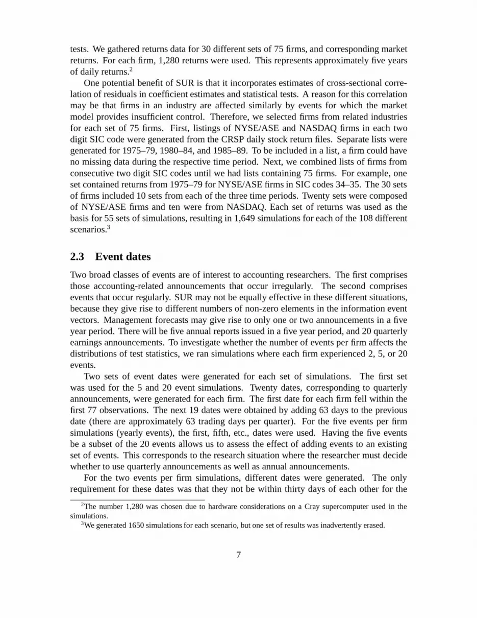
Two broad classes of events are of interest to accounting researchers. The first comprisesthose accounting-related announcements that occur irregularly. The second comprisesevents that occur regularly. SUR may not be equally effective in these different situations,because they give rise to different numbers of non-zero elements in the information eventvectors. Management forecasts may give rise to only one or two announcements in a fiveyear period. There will be five annual reports issued in a five year period, and 20 quarterlyearnings announcements. To investigate whether the number of events per firm affects thedistributions of test statistics, we ran simulations where each firm experienced 2, 5, or 20events.

Two sets of event dates were generated for each set of simulations. The first setwas used for the 5 and 20 event simulations. Twenty dates, corresponding to quarterlyannouncements, were generated for each firm. The first date for each firm fell within thefirst 77 observations. The next 19 dates were obtained by adding 63 days to the previousdate (there are approximately 63 trading days per quarter). For the five events per firmsimulations (yearly events), the first, fifth, etc., dates were used. Having the five eventsbe a subset of the 20 events allows us to assess the effect of adding events to an existingset of events. This corresponds to the research situation where the researcher must decidewhether to use quarterly announcements as well as annual announcements.

For the two events per firm simulations, different dates were generated. The onlyrequirement for these dates was that they not be within thirty days of each other for the

2The number 1,280 was chosen due to hardware considerations on a Cray supercomputer used in thesimulations.

3We generated 1650 simulations for each scenario, but one set of results was inadvertently erased.

7

same firm.The maximum number of events per firm in a given simulation was 20. Over the 55

sets of simulations based on a single set of firms, this implies that 1,100 dates per firm wereused as event dates. No attempt was made to insure that the dates for a given firm weredifferent across simulations.

2.4 Levels of abnormal performance

In order to determine the Type I error rates of the various statistics, simulations were runwhere no abnormal performance was introduced into the returns vectors. Simulated valuesused in the Ai vectors on event dates as measures of (false) information were uniformlydistributed [.00125,.00375] (mean of .0025).

To assess the powers of different statistics under the alternative hypothesis, three rangesof abnormal performance and associated information events were used: [.00125,.00375](mean of .0025), [.00375,.00625] (mean of .005), and [.0025,.0075] (mean of .005). Threedifferent ranges were used to assess how different levels of abnormal performance affect theability of SUR to detect stock price responses to information events. In these simulations, thesimulated values were used in the Ai vectors on event dates and were added to the respectivefirms’ returns vectors on corresponding days. This implies that the true coefficient relatingthe information variables to the abnormal returns was unity for all firms.

2.5 Numbers of firms

Accounting researchers are faced with questions regarding adequacy of sample size. InSUR, there are two sample size issues. The first one, how many events per firm are needed,has been discussed in a previous section. The second one involves the number of firms thatare needed for effective use of SUR. We did simulations with 3 different sample sizes, interms of numbers of firms. Each of the 30 sets of 75 firms was broken down into subsetsof 25, 50, and 75 firms. The models using 50 firms added 25 firms to the models using 25firms, and the models using all 75 firms added 25 firms to the 50 firm models. When 25additional firms were added to a model, the information event dates and values for the firmsalready in the model remained the same. This allows us to assess the effect of addingadditional firms to an existing data set, rather than confounding the addition of firms withthe effects of new event dates and abnormal returns for existing firms.

2.6 Event windows

Assessing the stock price change associated with an accounting information release is mademore difficult because the researcher may not know exactly when a piece of accountinginformation became known. This difficulty was overcome in studies based on marketmodel abnormal returns by using a cumulative abnormal return that covered a multidaywindow assumed to include the date of actual release of the information. Generally, longerevent windows in SUR are implemented by assigning the information value for a given

8

event to several consecutive elements in the information event vector. However, this doesnot accomplish the same thing that was accomplished with a cumulative abnormal return.Underlying the use of cumulative abnormal returns is the idea that the effect of (possiblyunidentified) confounding events occurring during the cumulation period will average outto zero, so the expected value of the cumulative abnormal return will be the abnormal returnassociated with the event of interest. Assigning the information value to several consecutiveevent dates in SUR may accomplish quite another thing. In effect, the researcher assumesthat the entire stock price change due to an accounting disclosure takes place rapidly, but isunable to identify exactly when the disclosure was made.4 Assume that all event windowsare two days in length (the information event vector has two consecutive non-zero valuesfor each event), and that the return of interest occurs on one of the two days. In terms ofequation (1), the portion of rit not explained by �i + �irmt has an expected value of zeroon non-event days, and is the desired abnormal return on the true event day. Hence, the i

coefficient will be estimated using observations half of which have the desired relation, andhalf of which in effect associate the information variable with a value of zero (or noise).Because i is estimated by minimizing the sum of squared residuals, it will be biasedtoward zero, and its standard error will be biased upwards, relative to the situation wherethe information variable is non-zero only on the “correct” date.

In order to assess the behavior of SUR in situations where the event date cannot beidentified exactly, two day and five day event windows are used, in addition to the one daywindow. In the two (five) day simulations, the information variable is assigned the non-zerovalue two (five) consecutive days, while the non-zero value is added as an abnormal returnto the actual return on only one of the two (five) days.5

3 Hypotheses tested and statistics used in the tests

There are two basic hypotheses tested in accounting event studies, both having to do with theassociation between stock price changes and information events. The first null hypothesisis that each of the i coefficients in (1) is equal to zero. The second null hypothesis isthat the average stock price response to the information events, across all firms and events,is equal to zero; i.e., there is no information disclosed in the information releases that isassociated with stock price changes, on average. Likelihood ratios, �2 statistics, several Fstatistics, and statistics based on sums of coefficients and associated standard errors havebeen proposed to test these hypotheses. Parks and Teets [1993] presents evidence on severalof these statistics. Here, we concentrate on three sets of F-statistics and statistics based onsums of coefficients and associated standard errors.

4There may be cases when the researcher assumes that the reaction to the announcement takes place overseveral days. In these cases, having non-zero information values for consecutive days may be appropriate.

5We always added the value to the first return in the multiday window. As the event dates are randomlygenerated, this should not affect the generalizability of our results to situations where the event window isconstructed to precede or surround the uncertain event date.

9

3.1 H01 : i = 0 8i

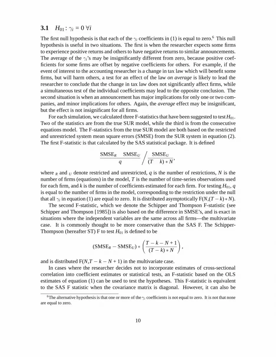
The first null hypothesis is that each of the i coefficients in (1) is equal to zero.6 This nullhypothesis is useful in two situations. The first is when the researcher expects some firmsto experience positive returns and others to have negative returns to similar announcements.The average of the i’s may be insignificantly different from zero, because positive coef-ficients for some firms are offset by negative coefficients for others. For example, if theevent of interest to the accounting researcher is a change in tax law which will benefit somefirms, but will harm others, a test for an effect of the law on average is likely to lead theresearcher to conclude that the change in tax law does not significantly affect firms, whilea simultaneous test of the individual coefficients may lead to the opposite conclusion. Thesecond situation is when an announcement has major implications for only one or two com-panies, and minor implications for others. Again, the average effect may be insignificant,but the effect is not insignificant for all firms.

For each simulation, we calculated three F-statistics that have been suggested to test H01.Two of the statistics are from the true SUR model, while the third is from the consecutiveequations model. The F-statistics from the true SUR model are both based on the restrictedand unrestricted system mean square errors (SMSE) from the SUR system in equation (2).The first F-statistic is that calculated by the SAS statistical package. It is defined

SMSER � SMSEU

q

,SMSEU

(T � k) � N,

where R and U denote restricted and unrestricted, q is the number of restrictions, N is thenumber of firms (equations) in the model, T is the number of time-series observations usedfor each firm, and k is the number of coefficients estimated for each firm. For testing H01, qis equal to the number of firms in the model, corresponding to the restriction under the nullthat all i in equation (1) are equal to zero. It is distributed asymptotically F(N,(T� k)�N).

The second F-statistic, which we denote the Schipper and Thompson F-statistic (seeSchipper and Thompson [1985]) is also based on the difference in SMSE’s, and is exact insituations where the independent variables are the same across all firms—the multivariatecase. It is commonly thought to be more conservative than the SAS F. The Schipper-Thompson (hereafter ST) F to test H01 is defined to be

(SMSER � SMSEU) �

T � k � N + 1(T � k) � N

!,

and is distributed F(N,T � k � N + 1) in the multivariate case.In cases where the researcher decides not to incorporate estimates of cross-sectional

correlation into coefficient estimates or statistical tests, an F-statistic based on the OLSestimates of equation (1) can be used to test the hypotheses. This F-statistic is equivalentto the SAS F statistic when the covariance matrix is diagonal. However, it can also be

6The alternative hypothesis is that one or more of the i coefficients is not equal to zero. It is not that noneare equal to zero.

10

expressed as1N

NXi=1

2i

�2 i

,

where N is the number of firms, the i are from equation (1), and �2 i

are the OLS estimatesof the variances of the i.7 This statistic, which we denote the Theil F, is distributedasymptotically F(N,(T � k) � N).

3.2 H02 :PN

i=1 i = 0

The second null hypothesis is that the average8 stock price response to the informationevents, across all firms and events, is equal to zero; i.e., there is no information disclosedin the information releases that is associated with stock price changes, on average. In caseswhere the effects of the information events are expected to be in the same direction for allfirms, this may provide a more powerful test than the previous test. This is because theaccumulation of many small effects, none significant in themselves, may be significant intotal.9

To test H02, we again calculated two F-statistics from the true SUR model. The SAS Fused to test H02 is again defined as

SMSER � SMSEU

q

,SMSEU

(T � k) � N.

For testing H02, q is one, the only constraint under the null being that the sum of the i

coefficients be zero. This statistic is distributed asymptotically F(1,(T � k) � N).The Schipper and Thompson F-statistic used to test H02 is simply

(SMSER � SMSEU),

and is distributed F(1,T � k) in the multivariate case.There are three statistics based on the consecutive equations model that can be used to test

H02. The first, which we again call the Theil F, is asymptotically distributed F(1,(T�k)�N).It can be calculated as �PN

i=1 i

�2

PNi=1 �

2 i

.

The final two statistics, which we call SUMT and SUMC, were used by Malatesta10

[1986]. SUMT is a sum of t-statistics, divided by the square root of the number of t-statistics

7See Theil, pp. 314-317, particularly problem 3.1.8Tests of

PNi=1 i = 0 and 1

N

PNi=1 i = 0 result in the same F statistic. It is convenient to drop the 1

N term.9Earlier abnormal returns studies generally tested this hypothesis. While offsetting effects could be handled

by creating separate portfolios for firms expected to be affected positively or negatively, this would still givestatistics based on groups of firms, rather than a statistic testing all firms individually, but simultaneously.

10SUMT and SUMC are the W** and Z** statistics in Malatesta. McDonald reports the W** statistic, butnot the Z** statistic.

11

in the sum:

SUMT =

NX

i=1

i

� i

!.pN,

where N is the number of firms. SUMT is distributed N(0,1) under the null hypothesis ofno stock price effect, on average, associated with the information events, and ignoring thecovariance structure of the firm returns.

SUMC is the sum of the i coefficients, divided by the square root of the sum of theirOLS variances:

SUMC =

NX

i=1

i

!, NX

i=1

�2 i

!(1/2)

.

SUMC is also distributed N(0,1), again assuming that firm returns are independent.

4 Results of simulations

In this section, we report on two aspects of the results of the simulations. First, we discussthe Type I error rates of the various statistics for each of the two hypotheses. Next, wediscuss the power of the statistics.

4.1 Type I errors: Rejections when no abnormal performance is in-troduced

4.1.1 H01 : i = 0 8i

In table 1 we present the Type I error rates for the three F-statistics used to test H01. AType I error occurs when the null hypothesis is rejected when no abnormal performancewas introduced into the returns series on the event dates.11 All of the rejection frequenciesare significantly above the nominal levels. Using a normal approximation to the binomialdistribution, and n=1649, the 95% confidence intervals should be [3.9%, 6.1%] for thenominal 5% rejection level, and [.5%, 1.5%] for the 1% rejection level. The null hypothesisis rejected far too often. At the nominal 5% level, rejection rates range from 9.2% to 33.9%for the SAS F, 8.2% to 23.5% for the ST F, and 6.9% to 20.3% for the Theil F. The bestcase at the 5% level occurs for the Theil F statistic for 20 events and 25 firms, using a 1day window. The rejection rate of 6.9% is about 3.5 standard deviations away from the 5%level. For the nominal 1% level, rejection rates are also high. For the SAS F, rejection ratesrange from a low of 3.5% to a high of 19.5%. Similar ranges for the ST F and the Theil Fare 2.9% to 11.9% and 2.7% to 9.6%. The best case at the 1% level again occurs for the

11It may be that the apparent over-rejections are due to our having non-zero elements in the Ai vectors thathappen to coincide with dates on which there actually were significant information events for the firms usedin the simulations. However, that is a strength of basing the simulations on real returns data, not a weakness.The researcher can never get a truly clean sample, where nothing else has affected the firms on the identifiedevent dates. Only by using returns drawn from such an information rich environment can we get a realisticidea about how the statistical methods will behave in practice.

12

Theil F, for 20 events and 25 or 75 firms, using a 1 day window. The rejection rate of 2.7%is almost 7 standard deviations from the nominal 1% level.

Note that the 2 event scenarios are independent of the 5 event scenarios, while the5 event scenarios are selected by choosing every 4th event from the 20 event scenarios.Hence, the 5 and 20 event scenarios are not independent. Also, the statistics themselvesare not independent. They are calculated from the same models, using the same returnsand simulated events. The statistics differ in whether they incorporate estimates of cross-sectional covariance. They also differ as to degrees of freedom used in finding critical valuesused to determine significance levels of the calculated statistics, although the statistics maybe asymptotically nearly the same.

There are a few regularities to be seen across the three panels. First, the more firmsthere are in the model, the worse over-rejection is. This holds true across all windows foralmost all numbers of events. Second, the Theil F statistic almost always has the lowestover-rejection rate, followed by the ST F, followed by the SAS F, regardless of number ofevents, firms, or window length. Third, for a given window length and number of firms,the highest over-rejection rate is generally for the 5 event scenario. Generally, the nexthighest is with 2 events, with 20 events being the lowest, but still very high compared to thenominal Type I error rates. The “best” window length is 5 for scenarios with 2 or 5 events,but is 1 for scenarios with 20 events.

4.1.2 H02 :PN

i=1 i = 0

Table 2 contains the empirical Type I error rates for the 5 statistics used to test H02, that theaverage of the i coefficients is zero. In general, the empirical Type I error rates for all ofthese statistics are much closer to the nominal levels than the error rates for the statisticsused to test H01. For scenarios with 2 or 20 events, only 14 out of the 180 different statisticsare outside the 95% confidence intervals. If the statistics were independent, we wouldexpect 9 to be outside the limits of a 95% confidence interval, strictly due to chance, andthese statistics are not independent. Across all scenarios and all 5 statistics, rejection ratesat the 5% level, 2 or 20 events, range from 3.5% to 6.9%. At the 1% level, respective valuesare .4% to 1.7%.

For the scenarios with 5 events, the situation is very different. Only 14 of the 90 statisticspresented are within the 95% confidence interval limits. For 5 events, all of the statisticsexhibit high Type I error rates, ranging from 5.2% to 17.2% at the nominal 5% level and1.4% to 6.7% at the 1% level. Most of them lie outside the 95% confidence intervals of[3.9%,6.1%] and [.5%,1.5%]. We have no explanation for why the statistics do relativelywell with 2 and 20 events, but very poorly with 5 events. (Recall that the 20 event scenariosessentially take the 5 event scenarios and add an additional 15 events. Therefore, the 5 and20 event scenarios are not independent. Yet the 20 event statistics appear to be reasonablywell specified, while the 5 event statistics reject too often.)

Comparing the true SUR statistics, the rejection rates for the SAS F and the ST F areidentical for all scenarios presented. (See Appendix A for an explanation of this apparentequality.) Comparing the statistics calculated using the consecutive equation model, theTheil F and SUMC statistics have essentially identical rejection rates, differing in only 2

13

cells presented.At the 5% level, the 95% confidence interval for n=1649 is about 4% to 6%. As shown in

table 2, the SUMC statistics reject the null less often than the SUMT statistics but for mostof the scenarios with 2 or 20 events per firm, the rejection frequencies for both statisticsare within the 95% band. Again, for the 5 events per firm scenarios, both statistics rejectsignificantly more often than would be expected based on the nominal size of the tests.The SUMT rejection rates are particularly high for some scenarios. There is no uniformbehavior with respect to the number of firms, or the window length.

Probably these statistics fail (lie outside the 95% confidence band) due to ignoring thecovariance structure. The statistics only fail by being above the top of the 95% confidenceband, probably indicating that for those cases ignoring the covariance structure producesstatistics a little too large.

4.2 Empirical distributions when no abnormal performance is intro-duced

In this section, we present the first and fifth percentiles of the empirical distributions of thestatistics when no abnormal performance is introduced. This is done in order to presentmeaningful power tables in the next section. Powers of statistical tests must be evaluatedfor specific Type I error levels. Researchers are generally interested in powers of tests givenType I error rates of 5% or 1%. Since statistics for some scenarios had Type I error ratesmuch higher than indicated by the nominal size, power tables for nominal Type I error ratesof 5% and 1% would not be very informative. To provide more meaningful power tablesin the next section, we used as critical values the first and fifth percentiles of the empiricaldistributions generated when no abnormal performance was introduced. We present thoseempirical values in this section.

Rather than using the calculated F- or z-statistics, we work with the p-values of thosestatistics. The p-values are those associated with the calculated statistics and their theoreticaldistributions and degrees of freedom. This allows uniform interpretation of the empiricalcritical values given. That is, all empirical critical values are p-values, ranging between0 and 1, rather than being points from different distributions with different degrees offreedom.

Tables 3 and 4 present the first and fifth percentiles of the empirical distributions of thep-values of the statistics generated in the simulations where no abnormal performance wasintroduced. Table 3 presents the empirical critical p-values for the statistics used to testH01 : i = 0 8i; table 4 presents similar values for testing H02 :

PNi=1 i = 0.

Each cell entry is based on the empirical distribution of the 1,649 statistics generatedfor a specific scenario. Consider the cell in table 3, panel A, for the SAS F statistic testingwhether all of the i are equal to 0, for 2 events, 25 firms, window length 1 day, 5% leveltest. The p-values based on theoretical distributions were obtained for each of the SAS Fstatistics from the 1,649 simulations using 2 events, 25 firms, and a window length of 1day, where no abnormal performance was added to the firm return vectors on the (false)event dates. The value of 0.219 indicates that 5% of the p-values for these F statistics were

14

smaller than 0.219%. An F statistic with a p-value larger than 0.219% would not representa rejection of the null hypothesis at the 5% level, based on the empirical distribution.

Another way of looking at tables 3 and 4 is that if the p-values listed in each cell wereused as the critical values for rejecting the null hypothesis, the Type I error rates would beexactly 5% (1%) for all scenarios where no abnormal performance was introduced in thesimulation process.

4.2.1 H01 : i = 0 8i

The high Type I error rates presented in table 1 imply that the first and fifth percentiles ofthe empirical distributions of nominal p-values must be smaller than 1% and 5%. Table3 shows that, except for scenarios with 20 events per firm, the first and fifth percentilesare at least an order of magnitude smaller than the nominal 1% and 5% levels. Of thetrue SUR statistics, the ST F statistic is in general closer to the nominal values than is theSAS F. Empirical 5% rejection rates were achieved for the ST F by using p-values rangingfrom .047% to 2.421%. To achieve a 1% rejection rate, p-values ranging from 9E-6% to.404% were needed. For the SAS F, empirical p-values used to achieve 5% (1%) empiricalrejection rates ranged from .005% (1E-7%) to 1.868% (.276%). The empirical p-values forthe Theil F from the consecutive equations model are closer to the nominal p-values thanare the ST F at the 5% nominal level, but neither statistic dominates at the 1% nominallevel.

For all three statistics, for a given number of firms and window length, increasing thenumber of events per firm brings the empirical 5% and 1% points closer to the respectivenominal points. However, for a given number of events, adding firms moves the empiricalcritical values farther from the nominal values. That is, as more firms are added, smallercritical p-values must be used to achieve the same nominal size test. Finally, for scenarioswith 2 or 5 events per firm, increasing the window length brings the empirical criticalp-values up towards the nominal values, but for the 20 event scenarios, increasing windowlengths push the empirical critical p-values down, farther from the nominal values.

4.2.2 H02 :PN

i=1 i = 0

Table 4 presents the first and fifth percentiles of the distributions of p-values for the statisticsused to test whether the average of the coefficients is significantly different from zero.These points from the empirical distributions are closer to the nominal values than were therespective points for the statistics testing H01. The empirical values are generally below thenominal values, but not always. For scenarios with 20 events per firm, the empirical valuesare sometimes larger than the nominal values.

For a given number of firms and window length, scenarios with 2 or 20 events haveempirical values close to the nominal values, while the empirical values for 5 event scenariosare generally smaller. There is no consistency in the effect of adding firms for a given numberof events and window length. For 2 event scenarios, for a given number of firms, increasingthe window length brings the empirical critical values closer to the nominal values. Thereis no such consistency for the 5 and 20 event scenarios.

15

In summary, from both the tables of Type I error rates and the tables of the 5% and 1%points of the empirical distributions, it is clear that all of the statistics testing H01 reject toooften when no abnormal performance was introduced. The rejection rates for the statisticsused to test H02 are much closer to the nominal levels, although there is a slight tendencyto over-reject here as well. The next section looks at the other side of the coin—how oftenthe statistics reject the null of no abnormal performance when abnormal performance wasadded to the returns.

4.3 Power: Rejections of the null when abnormal performance is in-troduced

Given that the Type I error rates are generally excessive for the statistics examined, simplycalculating power as the percentage of rejections at the nominal 5% and 1% levels, whenabnormal performance is introduced, would be misleading. Therefore, we present in tables5 through 10 corrected power tables. The critical p-values used to determine rejection ornon-rejection of the null hypothesis are those presented in tables 3 and 4, discussed in theprevious section. All corrected power tables contain three panels, as three different rangesof abnormal performance were used in the simulations used to assess power. Abnormalperformance metrics used in the simulations reported in Panels A were drawn from auniform distribution over the range [.00125,.00375], with a mean of .0025. The secondrange, reported in panels B, was [.00375,.00625], with a mean of .005. The third range alsohad a mean of .005, but had a larger range, [.0025,.0075].

For all statistics for both hypotheses, for a given number of firms, number of events perfirm, and window length, the power of the tests increased as the mean level of abnormalreturn added on the event dates increased. That is, rejection rates for all scenarios andall statistics, panels A, where the abnormal returns have a mean of .0025, are lower thancorresponding cells from panels B and C, where the mean of the abnormal returns addedis .005, with differing ranges. The statistics are differentially sensitive to the variance ofabnormal returns added, as rejection rates are sometimes higher in panels B than C, andsometimes lower.

One final regularity can be seen across all corrected power tables. Up to this point, wehave discussed number of events per firm and number of firms in the model as separatevariables. We have done this primarily because these are separate concepts in the realmof accounting research. However, from a purely statistical point of view, changes in either(or both) change the total number of events in the model. An additional column has beeninserted in table 5, showing the total number of events in any given scenario. For all ofthe statistics for both tests, the rejection rates generally increase with the number of totalevents. However, the rates of increase differ across hypotheses tested, and will be discussedunder the appropriate hypothesis.

16

4.3.1 H01 : i = 0 8i

The first noteworthy item is that, after correcting for the different empirical rejection ratesunder the null hypothesis by using the scenario specific rejection rates given in table 3, thecorrected power rates for the SAS F and the ST F are identical to three decimal places. (SeeAppendix A for a reconciliation of these statistics.) Therefore, we present a combined tablefor the SAS and ST F statistics.

Tables 5 and 6 both show that, for a given number of events per firm and window length,adding additional firms increases the power of the tests. However, the increase in powerachieved by adding events for a given number of firms is much greater. For example, forthe ST F, using 75 firms instead of 25 firms, each with 2 events, increases the rejection ratefrom 6.2% to 6.6%. However, having 5 events rather than 2 events for 25 firms increasesthe rejection rate from 6.2% to 11.0%. In terms of total number of events in the model, 2events, 25 firms has 50 total events. Moving to 2 events, 75 firms gives 150 total events,while moving to 5 events, 25 firms only gives 125 total events. Yet the increase in power isgreater by increasing the number of events per firm.

Finally, window length has a dramatic effect on the powers of the test statistics in theinstances where the power for the (correctly specified) one day window is reasonably good.For example, the Theil F in panel B of table 6 rejects 45.5% of the time at the 5% level forthe 5 events, 75 firms scenario when a one day window is used. That drops to 26% when atwo day window is used, and to 11.2% when a five day window is used.

4.3.2 H02 :PN

i=1 i = 0

The corrected power rates for the SAS F and ST F for testing H02 are again identical to threedecimal places, after correcting for the difference between nominal and empirical Type Ierror rates. Therefore, we again present a combined table for the SAS and ST F statistics.

As was true for the statistics testing H01, the total number of events in the model isimportant. However, for H01, the number of events per firm was very important. Here, thatseems to be less true. For example, examine table 10, panel A, the 1% column under theone day window. The power with 2 events per firm, 75 firms, is 16.4%. For 5 events, 25firms, it is 13.1%. The total number of events goes down for the 5 events, 25 firms scenario,and the power declines. However, numbers of events per firm is not unimportant, either.In the 5% column for the same numbers of events, firms, and window length, the rejectionrate increases modestly, from 31.4% to 32.9%, even though the total number of events hasdecreased. Overall, the total number of events seems more important in determining powerfor tests of H02 than H01. In any case, increasing either the number of events for a givennumber of firms or increasing the number of firms for a given number of events per firmboth result in increases in power.

The effect of increases in window length is not as consistent for statistics testing H02

as for those testing H01. Increasing the window length results in substantial declines forall scenarios for the lowest level of added abnormal performance. For the higher level ofabnormal performance, both ranges, there is substantial decline for scenarios with 2 or 5events, or 20 events and 25 firms. However, for 20 events and 50 or 75 firms, the decreases

17

in power are small when moving from a 1 day window to a 2 day window. Moving to a 5day window results in substantial declines for all scenarios.

Finally, after correcting for the difference in Type I error rates, SUMT appears to bethe dominant statistic for testing H02. It always has higher power than the other statisticsexamined.

5 Research design and interpretation in light of simulationresults

In light of our simulations, what can one say about designing and interpreting results ofaccounting research studies using true SUR or the consecutive equations models? Basically,if one wishes to test hypotheses similar to our H01, that all firm-specific response coefficientsare equal to zero, one must use something like the models studied here. However, ourevidence indicates that one must use very conservative rejection regions, or the probabilityof Type I errors will be large. Furthermore, if one corrects for high Type I error rates byusing rejection regions based on the empirical distributions outlined here, power may bepoor, especially if the research examines infrequent events. For example, in table 5, panelA, for scenarios with 2 events per firm, 5% level test, rejection rates range from 6.2 to 6.6%,if the exact event date was known. With event date uncertainty, that range declines to 5.1to 6.4%. Since rejections of the null hypothesis in this table are based on the empiricalcritical p-values from table 3, approximately 5% of the simulations would have resulted inrejections even if no abnormal performance had been introduced. For scenarios with fewevents per firm, the power is barely above the number of rejections expected in the absenceof introduction of any abnormal performance. However, if the study focusses on recurringevents such as quarterly announcements, and there is only slight event date uncertainty, thepower is much better. For example, in the same column, if there are 20 events per firm,rejection rates range from 42.6% to 61.2%.

If the researcher is interested only in average effects, the true SUR and the consecutiveequations statistics are much better behaved. Type I error rates reported in table 2, whilestill generally too high, are nowhere near as high as reported in table 1 for tests of H01. Thepowers of the tests are also higher.

If one is only interested in the average effects, the tendency may be to use a moretraditional event study method, such as portfolio abnormal return analysis or cross-sectionalpooled regressions of abnormal returns on information variables. However, these methodsalso have drawbacks. In portfolio abnormal return analysis, the levels of (surprise in)accounting information cannot be included as explanatory variables. In cross-sectionalpooled regressions, constraining the coefficients to be the same for all firms or for groupsof firms can create problems.12 Our simulations indicate that true SUR or the consecutive

12Teets [1992] presents an example where inference from SUR and inference from a pooled cross-sectionalregression are opposite. Several differences between SUR and the pooled cross-sectional approach areexamined to see which one(s) drive the difference in inference. The constraint of equality of coefficientsunder the pooled cross-sectional method appears to drive the difference in inference.

18

equations model, both of which permit inclusion of levels of information and firm-specificcoefficients, may be acceptable alternatives, in terms of Type I error rates and power, fortests of average effects.

We chose the numbers of events per firm to be representative of situations encountered inaccounting research. First, the two events per firm scenario corresponds to infrequent events,such as management forecasts of earnings. Second, regular accounting announcementsoccur annually or quarterly. Over a five year period, that will give rise to 5 or 20 eventsper firm. To avoid problems with structural change in the sample firms, accountants havefrequently restricted their analysis to not more than 5 year periods. Our results suggestthat the powers of the test statistics are low for scenarios with only 2 events per firm.This suggests that SUR may not have sufficient power to correctly identify significantinformation events, after correcting for high Type I error rates, in studies of infrequentlyoccurring events. However, for studies using quarterly announcements, SUR may workacceptably.13

If the researcher has to choose between adding firms to the sample, where each firm willhave only a few events, or identifying additional events for firms already in the sample, ourresults suggest that either strategy will provide gains in power. If the research question hasto do with average effects, either strategy may work equally well. However, if the questionhas to do with simultaneous tests for all firms (our H01), finding additional events for theexistent sample firms will give greater increases in power.

We used different window lengths to determine the extent of the problem caused by eventdate uncertainty when using SUR. Our results suggest the way that event date uncertaintyis typically addressed in SUR can severely affect the test statistics. There is a substantialreduction in power upon moving to a 2 day window from a 1 day window, and a furtherreduction upon moving to a 5 day window. This reduction in power suggests that SUR astypically implemented may not be appropriate when there is major event date uncertainty.14

Finally, what do our results imply about the choice between the true SUR and consecutiveequations models? On the whole, there doesn’t seem to be a lot to recommend one overthe other, empirically. For testing H01, the ST F statistic generally has higher correctedpower than the Theil F from the consecutive equations model, but in many of the scenarios,they are very similar. In tests of H02, the SUMT statistic from the consecutive equationsmodel had the highest power in all scenarios. The near equality of the methods may be dueto the noise in the cross-sectional covariance estimation process offsetting the gains fromincorporating covariance estimates in the coefficient estimates and statistical tests.

13This discussion assumes that the average abnormal returns associated with the different frequency eventsare similar. If the infrequent events are associated with large abnormal returns, and the quarterly announce-ments are associated with small abnormal returns, these conclusions may not hold.

14There are several ways that multiple day event windows could be implemented using firm-specific models.First, if the researcher doesn’t need to incorporate cross-sectional correlation, firm-specific models based onequation (1) could be estimated with single day returns outside the event periods and multiple day event periodreturns, using WLS instead of OLS. If the researcher wants to incorporate cross-sectional correlation, andevents are on the same day for all firms, SUR can be used after appropriately scaling the multiple day firmand market returns. Finally, if events happen at different times for different firms, leading to nonsynchronousmultiple day event period returns, a method suggested by Marais [1986] may be used.

19

6 Directions for future work

This simulation study of SUR examined situations where events occurred for different firmsat (possibly) different times. It did not examine the situation where a sequence of events(possibly) affects a number of firms on the same event dates. It is in this situation that theSchipper Thompson F statistics are theoretically exact. It would be interesting to simulatethis situation, to see if the ST statistics have better Type I error rates and power. Thiswould provide evidence on whether the over-rejection when no abnormal performance wasintroduced is due to the theoretical distributions holding only asymptotically, or due toleptokurtosis of the returns.

Alternatively, one could generate normally distributed data to use in place of the actualreturns data used in this study. Simulations based on this data could provide evidence onthe effects of non-normality. One could also use much longer time series of generated data,without having to worry about nonstationarity. This could provide evidence on the effectsof the distributions holding only asymptotically.

In these simulations, all coefficients were positive, and equal to unity. In this case testsof the second hypothesis, on the average of the coefficients, should be more powerful thantests of the first hypothesis. Simulations where there is variation across the coefficientsrelating information to stock prices would give additional evidence on the use of SUR ininformation event studies.

Finally, comparing pooled cross-sectional methods, portfolio abnormal return analysis,and SUR under a variety of simulated conditions might provide evidence about whenresearchers could rely on a method, and when assumptions of that method are violatedseriously enough that different methods must be contemplated.

20

A Reconcilation of SAS F and ST F

The SAS F used to test H01 : i = 0 8i is defined as SMSER�SMSEUq

.SMSEU(T�k)�N , and is

distributed asymptotically F(N,(T � k) � N), while the ST F is defined ST = (SMSER �SMSEU)�

�T�k�N+1(T�k)�N

�and is distributed asymptotically F(N,T�k�N +1) in the multivariate

case.Define SMSEDF = SMSEU

(T�k)�N . Consider the ratio of the SAS F to the ST F. It is1

SMSEDF1277

1278�N , since T is 1280 for all simulations, and k is 3. Based on our simulations,

the means (standard deviations) of the ratio SAS FST F for N = 25, 50, and 75 are 1.0192

(.000022), 1.040 (.000044) and 1.0616 (.000037). The slight variation in the ratio is dueto the 1

SMSEDF factor. Asymptotically, SMSEDF! 1. The mean (standard deviation) ofSMSEDF for N = 25, based on 59,364 simulations using 25 firms, is .999967 (.000021).Respective numbers for 50 and 75 firms are .999935 (.000042) and .999916 (.000035). TheSAS F is essentially a constant multiple of the ST F; the multiple depends only on the Nparameter.

The SAS F is compared to the F(N, (T � k) �N) distribution, and the ST F is comparedto the F(N, T� k�N + 1) distribution. However, if the denominator degrees of freedom arelarge (greater than 1000), the F distribution is essentially only dependent on its numerator,a �2 divided by its degrees of freedom. Hence, both the SAS F and ST F are compared toa �2

N divided by N. For N = 25, 50, and 75, the critical values for a nominal 5% test are1.506, 1.350, and 1.293.

Since SAS F � 1.0192 ST F for N = 25, and both statistics are compared to the samecritical value, the empirical rejection rates are different, and always higher for SAS F.Assume that a simulation using 25 firms resulted in an ST F of 1.505. Based on the nominal5% critical value of 1.506, this ST F would not lead to rejection of the null. However, thecorresponding SAS F would be approximately 1.535 (since SMSEDF is not exactly 1), andwould lead to rejection of the null.

The reason the rejection rates based on the empirical distributions are the same is that theempirical critical values compensate for the factor relating the SAS F to the ST F. Considerthe 5% critical values from table 3 for the SAS F and the ST F, for the scenario with 2events per firm, 25 firms, using a 1 day window. The SAS F critical p-value is .219%,which translates to an F of 1.9973, while the ST F critical p-value is .325%, which has acorresponding F value of 1.9596. The ratio of these critical values is approximately 1.0192,which is the same as the mean multiplication factor (for 25 firms) used to translate the STF into the SAS F. The empirical critical values offset the multiplication factor by which thetwo statistics differ.

The SAS F and ST F statistics used to test H02 :PN

i=1 i = 0 are even more closely related.The SAS F is as defined for the test of H01, but q is now equal to unity. The ST F is simplySMSER � SMSEU. As indicated previously, SMSEDF ! 1 asymptotically. Therefore, theSAS F and ST F have almost identical values. Although the degrees of freedom used todetermine critical values differ across the two statistics (1 and (T � k) � N for the SAS Fand 1 and T � k for the ST F), the denominator degrees of freedom are large enough bothstatistics are essentially compared to a �2

1. The minor effect of SMSEDF is offset by the

21

small differences in the p-values of the empirical critical values presented in table 4.

22

References

[1] Stephen J. Brown and Jerold B. Warner. Measuring security price performance.Journal of Financial Economics, 205–58, June, 1980.

[2] Stephen J. Brown and Jerold B. Warner. Using daily stock returns. Journal of FinancialEconomics, 14(1):3–31, 1985.

[3] Cynthia J. Campbell and Charles E. Wasley. Measuring security price performanceusing daily NASDAQ security returns. October 1991. Working paper, WashingtonUniversity in St. Louis.

[4] C.S. Agnes Cheng, William S. Hopwood, and James C. McKeown. Non-linearityand specification problems in unexpected earnings response regression model. TheAccounting Review, 67(3):579–598, July 1992.

[5] Daniel W. Collins and Warren T. Dent. A comparison of alternative testing methodolo-gies used in capital market research. Journal of Accounting Research, 22(1):48–84,Spring 1984.

[6] Thomas Dyckman, Donna Philbrick, and Jens Stephan. A comparison of event studymethodologies using daily stock returns: a simulation approach. Journal of AccountingResearch, Supplement, 22:1–30, 1984.

[7] P. Malatesta. Measuring abnormal performance: the event parameter approach usingjoint generalized least squares. Journal of Financial and Quantitative Analysis, 21:27–38, March 1986.

[8] M. Laurentius Marais. On detecting abnormal returns to a portfolio of nonsyn-chronously traded securities. 1986. Working paper, University of Chicago.

[9] Bill McDonald. Event studies and systems methods: some additional evidence.Journal of Financial and Quantitative Analysis, 22(4):495–504, December, 1987.

[10] Robert P. Parks and Walter R. Teets. Evidence on misspecification of seemingly un-related regression statistics. September 1993. Working paper, Washington Universityin St. Louis.

[11] Grace Pownall, Charles Wasley, and Gregory Waymire. The stock price effects ofalternative types of management earnings forecasts. September 1992. WashingtonUniversity.

[12] Grace Pownall and Gregory Waymire. Voluntary disclosure choice and earningsinformation transfer. Journal of Accounting Research, 27 Supplement:85–105, 1989a.

[13] Grace Pownall and Gregory Waymire. Voluntary disclosure credibility and securi-ties prices: evidence from management earnings forecasts, 1969-1973. Journal ofAccounting Research, 27(2):227–245, Autumn, 1989b.

23

[14] Katherine Schipper and Rex Thompson. The impact of merger-related regulationsusing exact distributions of test statistics. Journal of Accounting Research, 23:408–15, 1985.

[15] Walter R. Teets. An empirical investigation into the association between stock marketresponses to earnings announcements and regulation of electric utilities. Forthcomingin Journal of Accounting Research, Autumn, 1992.

[16] Walter R. Teets. A methodological consideration on the choice between event studyestimation procedures. November 1991. Working paper, University of Illinois atUrbana-Champaign.

[17] A. Zellner. An efficient method of estimating seemingly unrelated regressions and testsfor aggregation bias. Journal of the American Statistical Association, 57:348–368,1962.

24

Table 1: Type I error rates: Percentage of 1,649 simulations whereH01 : i = 0 8i was rejected when no abnormal performance was introduced.

Modela: rit = �i + �i rmt + i Ait + "it

Panel A: SAS F Statisticd

Number of Number of 1 Day Windowb 2 Day Windowb 5 Day Windowb

events/firm firms (N) 5%c 1% 5% 1% 5% 1%2 25 13.2 7.7 12.7 7.3 10.7 5.52 50 19.6 11.5 18.1 9.8 13.9 7.82 75 25.5 15.0 23.4 13.9 19.3 11.6

5 25 14.9 7.6 15.1 7.0 12.5 4.85 50 23.4 12.0 24.9 12.3 18.5 8.45 75 31.2 18.3 33.9 19.5 25.5 13.2

20 25 9.2 3.5 11.3 3.8 12.6 4.720 50 13.6 5.0 18.0 6.9 16.7 7.320 75 21.2 9.7 23.7 9.9 22.0 10.6

Panel B: Schipper-Thompson F Statistice

Number of Number of 1 Day Window 2 Day Window 5 Day Windowevents/firm firms (N) 5% 1% 5% 1% 5% 1%

2 25 12.0 7.0 11.6 6.9 9.7 5.02 50 15.7 9.0 14.4 7.7 11.5 5.92 75 17.9 10.4 16.2 9.7 13.7 7.2

5 25 13.7 6.5 13.7 6.0 10.9 4.35 50 18.1 8.7 19.3 9.0 13.6 6.15 75 21.9 10.7 23.5 11.9 16.6 8.4

20 25 8.2 3.0 9.6 2.9 10.9 3.520 50 9.7 3.5 12.7 4.2 13.4 5.020 75 12.4 4.1 14.1 5.2 12.9 5.5

Panel C: Theil F-statisticf


2 25 12.2 7.0 11.0 6.6 9.3 4.82 50 14.3 8.5 13.6 7.5 10.4 5.42 75 14.5 8.7 13.2 7.9 11.9 6.2

5 25 12.9 6.4 13.3 5.8 11.5 5.05 50 14.9 7.9 17.5 8.4 14.7 7.25 75 17.2 8.6 20.3 9.6 16.1 7.9

20 25 6.9 2.7 9.4 3.0 11.7 4.120 50 8.5 3.0 11.2 3.5 12.9 4.720 75 8.9 2.7 10.9 3.8 11.0 3.8

25

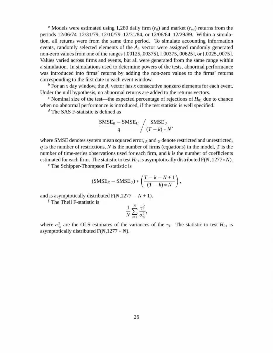
a Models were estimated using 1,280 daily firm (rit) and market (rmt) returns from theperiods 12/06/74–12/31/79, 12/10/79–12/31/84, or 12/06/84–12/29/89. Within a simula-tion, all returns were from the same time period. To simulate accounting informationevents, randomly selected elements of the Ait vector were assigned randomly generatednon-zero values from one of the ranges [.00125,.00375], [.00375,.00625], or [.0025,.0075].Values varied across firms and events, but all were generated from the same range withina simulation. In simulations used to determine powers of the tests, abnormal performancewas introduced into firms’ returns by adding the non-zero values to the firms’ returnscorresponding to the first date in each event window.

b For an x day window, the Ai vector has x consecutive nonzero elements for each event.Under the null hypothesis, no abnormal returns are added to the returns vectors.

c Nominal size of the test—the expected percentage of rejections of H01 due to chancewhen no abnormal performance is introduced, if the test statistic is well specified.

d The SAS F-statistic is defined as

SMSER � SMSEU

q

,SMSEU

(T � k) � N,

where SMSE denotes system mean squared error, R and U denote restricted and unrestricted,q is the number of restrictions, N is the number of firms (equations) in the model, T is thenumber of time-series observations used for each firm, and k is the number of coefficientsestimated for each firm. The statistic to test H01 is asymptotically distributed F(N, 1277�N).

e The Schipper-Thompson F-statistic is

(SMSER � SMSEU) �

T � k � N + 1(T � k) � N

!,

and is asymptotically distributed F(N,1277� N + 1).f The Theil F-statistic is

1N

NXi=1

2i

�2 i

,

where �2 i

are the OLS estimates of the variances of the i. The statistic to test H01 isasymptotically distributed F(N,1277 � N).

26

Table 2: Type I error rates: Percentage of 1,649 simulations whereH02 :

PNi=1 i = 0 was rejected when no abnormal performance was introduced

Model: rit = �i + �i rmt + i Ait + "it

Panel A: SAS F Statistica


2 25 5.6 1.7 5.5 1.5 4.5 1.12 50 5.6 1.6 5.1 1.3 4.7 1.02 75 5.9 1.4 5.2 1.4 4.5 1.0

5 25 5.3 2.0 6.1 1.4 5.8 1.65 50 6.8 1.6 6.5 1.8 6.8 1.85 75 6.4 2.2 6.5 1.5 7.9 2.2

20 25 5.4 0.9 6.2 0.7 4.8 1.020 50 5.3 1.2 5.5 1.0 5.4 1.320 75 5.9 1.3 5.9 1.3 5.3 1.0

Panel B: Schipper Thompson F Statisticb


2 25 5.6 1.7 5.5 1.5 4.5 1.12 50 5.6 1.6 5.1 1.3 4.7 1.02 75 5.9 1.4 5.2 1.4 4.5 1.0

5 25 5.3 2.0 6.1 1.4 5.8 1.65 50 6.8 1.6 6.5 1.8 6.8 1.85 75 6.7 2.2 6.5 1.5 7.9 2.2

20 25 5.4 0.9 6.2 0.7 4.8 1.020 50 5.3 1.2 5.5 1.0 5.4 1.320 75 5.9 1.3 5.9 1.3 5.3 1.0

Panel C: Theil F Statisticc


2 25 5.4 1.2 5.0 1.3 4.1 1.22 50 4.4 1.1 4.4 0.9 3.7 0.82 75 4.5 0.7 4.4 0.8 3.5 0.6

5 25 5.2 1.8 5.8 1.7 6.7 2.15 50 6.3 2.2 7.3 2.4 10.0 3.25 75 7.0 2.0 7.7 2.4 12.4 4.4

20 25 4.7 0.6 5.2 0.4 4.5 1.020 50 4.5 1.0 4.7 0.8 4.9 1.020 75 4.9 0.8 4.9 0.8 4.6 1.0

27

Panel D: SUMTd


2 25 6.9 1.3 6.2 1.2 5.0 1.52 50 5.1 1.1 5.2 1.0 4.5 1.22 75 5.6 1.0 5.4 0.8 4.1 0.7

5 25 6.5 1.7 7.2 2.1 8.6 3.05 50 7.0 2.5 9.3 3.0 13.2 4.95 75 7.0 2.4 10.5 2.7 17.2 6.7

20 25 5.0 1.0 4.9 1.0 5.8 1.320 50 4.9 0.8 4.6 1.1 5.6 1.520 75 4.1 1.0 5.4 1.0 6.6 1.4

Panel E: SUMCe


2 25 5.4 1.4 5.0 1.3 4.1 1.22 50 4.4 1.1 4.4 0.9 3.7 0.82 75 4.5 0.7 4.4 0.8 3.5 0.6

5 25 5.2 1.8 5.8 1.7 6.7 2.15 50 6.3 2.2 7.3 2.4 10.0 3.25 75 7.0 2.0 7.7 2.4 12.4 4.4

20 25 4.7 0.6 5.2 0.5 4.5 1.020 50 4.5 1.0 4.7 0.8 4.9 1.020 75 4.9 0.8 4.9 0.8 4.6 1.0

See notes to table 1 for definitions of symbols and description of model.a See notes to table 1 for formula. The statistic to test H02 is asymptotically distributed

F(1,(T � k) � I).b Statistic is calculated as SMSER – SMSEU , and is asymptotically distributed F(1,T�

k).c Statistic is calculated

�PNi=1 i

�2 .PNi=1 �

2 i

, and is distributed asymptotically F(1,(T�k) � I).

d Statistic is calculated�PN

i=1 i

� i

�.pN, and is distributed asymptotically N(0,1).

e Statistic is calculated�PN

i=1 i

��PNi=1 �

2 i

�(1/2)and is distributed asymptotically

N(0,1).

28

Table 3: First and fifth percentiles of empirical distributions of p-values ofstatistics testing H01 : i = 0 8i. Each distribution based on 1,649

simulations where no abnormal performance was introduced.


Panel A: SAS F statistic


2 25 0.219b <0.001 0.190 <0.001 0.735 <0.0012 50 0.017 <0.001 0.063 <0.001 0.272 <0.0012 75 0.005 <0.001 0.007 <0.001 0.062 <0.001

5 25 0.347 0.002 0.485 0.001 1.041 0.0015 50 0.083 <0.001 0.089 <0.001 0.239 0.0025 75 0.014 <0.001 0.017 <0.001 0.037 <0.001

20 25 1.868 0.128 1.430 0.276 1.047 0.09320 50 0.966 0.050 0.580 0.029 0.438 0.01020 75 0.297 0.023 0.211 0.009 0.198 0.003

Panel B: Schipper-Thompson F Statistic


2 25 0.325 <0.001 0.285 <0.001 1.010 0.0012 50 0.059 <0.001 0.186 <0.001 0.658 0.0012 75 0.047 <0.001 0.063 <0.001 0.357 <0.001

5 25 0.501 0.004 0.685 0.002 1.400 0.0025 50 0.236 0.001 0.251 0.002 0.589 0.0105 75 0.106 0.001 0.129 0.002 0.237 0.004

20 25 2.421 0.197 1.885 0.404 1.408 0.14620 50 1.974 0.151 1.271 0.096 0.996 0.03620 75 1.240 0.162 0.947 0.078 0.898 0.033

Panel C: Theil F Statistic


2 25 0.386 <0.001 0.367 <0.001 1.140 <0.0012 50 0.126 <0.001 0.218 <0.001 0.758 0.0012 75 0.090 <0.001 0.092 <0.001 0.600 <0.001

5 25 0.464 0.002 0.707 0.002 0.997 0.0025 50 0.247 <0.001 0.262 0.001 0.481 0.0035 75 0.189 0.001 0.172 0.001 0.215 0.007

20 25 2.964 0.156 1.968 0.340 1.517 0.11620 50 2.582 0.128 1.703 0.110 1.219 0.07920 75 2.195 0.227 1.638 0.096 1.455 0.029

See notes to table 1 for definitions.

29

Table 4: First and fifth percentiles of empirical distributions of p-values ofstatistics testing H02 :

PNi=1 i = 0. Each distribution based on 1,649

simulations where no abnormal performance was introduced.


Panel A: SAS F Statistic


2 25 4.044a 0.424 4.626 0.634 6.023 0.6862 50 4.154 0.810 4.947 0.815 5.237 1.0222 75 4.194 0.791 4.795 0.768 5.349 0.885

5 25 4.752 0.408 4.114 0.414 4.342 0.3765 50 3.530 0.497 3.872 0.458 3.592 0.5185 75 3.622 0.269 3.574 0.756 2.824 0.352

20 25 4.435 1.156 4.331 1.296 5.313 0.90420 50 4.661 0.852 4.649 1.063 4.574 0.69920 75 4.285 0.707 4.260 0.650 4.423 1.019

Panel B: Schipper-Thompson F Statistic


2 25 4.064 0.430 4.646 0.642 6.046 0.6952 50 4.174 0.820 4.968 0.825 5.259 1.0332 75 4.215 0.801 4.817 0.778 5.372 0.895

5 25 4.772 0.415 4.134 0.421 4.363 0.3825 50 3.549 0.504 3.892 0.466 3.612 0.5265 75 3.643 0.275 3.594 0.766 2.842 0.358

20 25 4.456 1.168 4.351 1.308 5.334 0.91520 50 4.683 0.862 4.671 1.074 4.596 0.70920 75 4.306 0.716 4.281 0.659 4.445 1.030

Panel C: Theil F Statistic


2 25 4.614 0.483 5.015 0.519 6.070 0.6642 50 5.434 0.948 5.685 1.032 6.937 1.3862 75 5.375 1.330 5.686 1.106 6.788 1.717

5 25 4.657 0.356 4.179 0.369 3.634 0.2675 50 3.340 0.385 2.932 0.234 1.674 0.1655 75 3.297 0.356 2.653 0.480 1.160 0.090

20 25 5.477 1.375 4.934 1.578 5.509 1.04620 50 5.680 0.922 5.153 1.354 5.158 1.00020 75 5.329 1.228 5.091 1.044 5.174 1.002

30

Panel D: SUMT


2 25 3.903 0.880 3.841 0.804 5.004 0.5762 50 4.586 0.895 4.852 1.002 5.545 0.8532 75 4.102 0.924 4.900 1.344 5.703 1.435

5 25 3.582 0.399 3.506 0.407 2.567 0.1575 50 2.498 0.300 2.072 0.235 1.047 0.0945 75 3.376 0.302 2.047 0.462 0.579 0.061

20 25 4.959 1.054 5.252 0.945 4.420 0.64420 50 5.187 1.145 5.233 0.961 4.527 0.51320 75 6.162 1.060 4.490 0.996 3.739 0.733

Panel E: SUMC


2 25 4.618 0.488 5.040 0.524 6.127 0.6742 50 5.436 0.989 5.688 1.040 6.979 1.4182 75 5.400 1.340 5.702 1.145 6.923 1.720

5 25 4.664 0.367 4.225 0.414 3.642 0.2985 50 3.360 0.391 2.940 0.264 1.690 0.1725 75 3.344 0.432 2.655 0.492 1.173 0.094

20 25 5.506 1.376 4.936 1.607 5.527 1.10320 50 5.706 1.014 5.193 1.378 5.188 1.06720 75 5.361 1.238 5.100 1.059 5.245 1.007

See notes to table 1 for model description.See notes to table 2 for statistic definitions.aAll p-values are expressed as percentages

31

Table 5: Power: Percentage of 1,649 simulations where H01 : i = 0 8i was rejected by theSAS and Schipper Thompson F-statistics when abnormal performance was introduced

Rejections based on empirical distributions summarized in Table 3


Panel A: Level 1, Abnormal returns from [.00125,.00375]

Number of Number of Events 1 Day Window 2 Day Window 5 Day Windowevents/firm firms (N) � firms 5% 1% 5% 1% 5% 1%

2 25 50 6.2 1.3 5.1 1.0 5.2 1.12 50 100 6.4 1.3 6.4 1.2 5.6 1.02 75 150 6.6 1.2 5.9 1.2 6.0 1.3

5 25 125 11.0 2.5 8.9 1.3 6.7 1.25 50 250 15.5 3.2 9.9 2.1 6.4 1.65 75 375 17.6 4.7 10.9 2.7 7.0 1.6

20 25 500 42.6 27.6 23.9 14.4 10.4 3.020 50 1000 56.2 40.6 34.9 20.1 14.4 3.120 75 1500 61.2 48.9 40.2 25.6 16.9 4.1

Panel B: Level 2, Abnormal returns from [.00375,.00625]


2 25 11.5 1.5 6.7 1.4 5.8 1.52 50 13.8 2.9 9.2 1.5 6.9 1.32 75 19.5 3.9 9.9 1.5 7.3 1.3

5 25 35.7 15.1 20.7 4.4 11.8 1.55 50 48.2 27.9 30.1 11.9 13.8 3.25 75 52.5 35.7 34.8 18.3 14.0 3.9

20 25 87.0 73.9 62.3 51.1 31.5 18.220 50 94.5 89.5 76.0 60.2 41.3 25.720 75 97.2 94.2 81.5 70.5 47.6 32.0

Panel C: Level 3, Abnormal returns from [.0025,.0075]


2 25 12.7 1.8 6.9 1.6 5.9 1.32 50 15.7 4.0 10.2 1.6 6.9 1.52 75 20.4 4.9 10.6 1.8 7.2 1.5

5 25 37.6 17.2 21.5 4.9 12.3 1.55 50 49.9 30.0 31.5 13.3 14.7 3.85 75 54.4 37.7 36.6 20.3 15.7 4.6

20 25 87.9 76.8 64.4 52.7 32.7 19.720 50 95.5 90.4 78.0 62.6 43.0 27.220 75 97.5 95.3 83.0 73.0 48.5 33.4


32

Table 6: Power: Percentage of 1,649 simulations where H01 : i = 0 8i wasrejected by Theil F-statistic when abnormal performance was introduced





2 25 6.1 1.3 5.7 1.0 5.3 1.02 50 7.0 1.4 5.8 1.2 5.6 1.02 75 6.8 1.3 5.6 1.1 5.8 1.1

5 25 10.7 1.9 9.2 1.6 6.9 1.25 50 15.0 2.2 9.9 1.6 7.5 1.35 75 18.7 4.8 11.6 2.5 7.2 2.4

20 25 42.6 25.6 23.7 12.9 11.1 2.920 50 54.0 37.7 33.5 18.2 13.6 4.020 75 59.9 46.0 40.1 22.4 16.2 3.3



2 25 9.0 1.3 6.4 1.5 5.5 1.02 50 9.6 1.9 7.2 1.4 6.5 1.12 75 11.3 2.2 6.9 1.2 6.9 1.2

5 25 24.4 5.8 16.2 2.5 9.6 1.55 50 38.5 11.4 20.1 3.7 10.9 2.25 75 45.5 21.8 26.0 7.6 11.2 3.8

20 25 86.0 69.3 56.1 41.7 21.9 8.820 50 95.0 87.0 72.8 55.1 31.2 14.820 75 97.1 94.1 79.3 64.2 39.5 15.3



2 25 12.6 1.9 7.7 1.5 6.3 1.22 50 16.1 3.1 10.1 1.5 7.0 1.52 75 19.5 4.4 9.3 1.6 7.6 1.5

5 25 37.5 15.3 22.7 5.6 11.9 1.85 50 48.8 26.9 32.3 10.0 15.7 3.25 75 54.5 36.5 37.3 19.2 16.3 7.1

20 25 88.1 74.3 63.0 51.2 32.4 17.920 50 95.9 89.1 77.5 61.1 42.6 28.020 75 97.6 94.6 82.7 69.8 48.6 30.7


33

Table 7: Power: Percentage of 1,649 simulations where H02 :PN

i=1 i = 0 was rejected bythe SAS and Schipper Thompson F-statistic when abnormal performance was introduced





2 25 13.6 4.3 10.0 3.3 7.2 1.52 50 23.2 10.7 15.9 5.5 9.3 2.92 75 31.3 15.8 20.2 7.6 10.9 2.7

5 25 32.9 13.8 20.9 6.2 13.6 3.35 50 50.4 32.4 34.0 16.1 20.4 7.75 75 60.1 37.2 43.6 26.8 24.3 9.6

20 25 67.3 51.6 44.5 33.1 24.1 11.720 50 87.0 74.1 66.6 51.0 36.5 20.320 75 92.9 83.7 75.1 59.6 47.1 31.5



2 25 41.0 19.1 26.4 11.1 14.3 3.52 50 60.5 44.5 43.5 24.8 21.6 10.02 75 69.5 55.4 52.6 33.7 30.4 13.6

5 25 70.6 46.9 50.9 28.1 30.5 11.05 50 86.4 73.1 70.2 50.5 48.0 28.05 75 92.9 80.1 79.4 67.7 56.1 36.2

20 25 95.5 91.4 82.7 74.0 57.1 39.420 50 99.5 98.5 95.6 90.5 75.4 58.520 75 99.8 99.8 98.2 95.1 85.3 73.5



2 25 38.9 17.8 25.5 10.4 13.5 3.32 50 58.5 41.5 41.0 24.6 19.5 9.52 75 67.7 52.8 49.8 32.1 28.9 12.5

5 25 71.4 48.2 51.8 28.1 30.7 11.35 50 86.5 73.1 70.5 51.4 48.5 28.25 75 93.1 80.5 80.5 67.9 56.1 36.9

20 25 95.9 92.5 84.1 75.4 58.2 41.420 50 99.6 98.8 96.2 91.5 77.6 60.320 75 99.8 99.8 98.5 95.8 86.8 75.3


34


i=1 i = 0 wasrejected by Theil F-statistic when abnormal performance was introduced





2 25 14.5 4.2 10.3 2.4 6.9 1.52 50 24.8 10.2 16.5 5.5 10.2 3.22 75 31.4 16.4 20.6 8.0 11.2 3.8

5 25 32.9 13.1 21.4 6.7 13.5 3.15 50 50.9 29.3 33.7 13.3 17.0 6.45 75 61.8 39.5 43.0 24.7 21.2 7.6

20 25 68.0 52.6 44.9 32.3 23.2 10.720 50 87.1 71.7 64.0 50.2 34.2 19.020 75 92.6 84.9 73.6 58.5 41.6 25.1



2 25 33.4 11.7 20.6 5.7 11.1 2.12 50 55.4 33.9 34.7 16.6 18.1 7.02 75 66.0 49.5 43.8 23.9 23.7 10.2

5 25 67.3 36.7 44.1 18.8 25.3 7.35 50 85.7 67.0 65.1 39.2 36.4 16.35 75 92.8 81.7 77.0 61.0 44.3 21.7

20 25 95.5 91.0 80.8 69.9 48.9 29.720 50 99.5 98.6 95.1 89.7 68.9 51.120 75 99.8 99.8 98.2 95.6 80.8 64.7



2 25 39.0 17.5 25.4 9.2 13.0 3.12 50 60.2 41.0 41.2 22.7 21.8 9.82 75 67.7 54.3 49.5 31.4 29.5 14.7

5 25 71.4 47.4 52.6 27.2 31.0 10.75 50 87.0 70.3 70.3 47.5 44.3 23.25 75 93.6 82.7 79.0 65.9 51.5 31.7

20 25 96.1 92.2 84.1 75.3 57.4 40.820 50 99.6 98.7 96.2 91.0 73.6 59.620 75 99.9 99.8 98.5 96.2 83.1 69.6


35


i=1 i = 0 wasrejected by SUMT statistic when abnormal performance was introduced





2 25 021.0 09.3 012.9 05.8 08.2 02.12 50 36.5 21.2 23.1 10.1 12.9 3.52 75 44.6 28.4 29.7 16.7 16.7 6.7

5 25 45.3 23.1 30.1 12.1 16.4 4.65 50 63.3 43.5 44.8 25.2 23.2 10.25 75 75.7 55.8 56.2 40.3 29.3 14.4

20 25 81.4 67.1 60.3 43.7 31.0 14.320 50 94.5 89.5 78.7 63.3 46.9 27.020 75 98.6 94.7 86.2 75.3 56.1 40.4



2 25 54.9 38.1 35.1 20.4 19.6 5.32 50 74.1 58.8 56.0 38.4 32.1 14.62 75 82.2 69.6 65.9 51.8 41.9 26.2

5 25 80.7 64.2 64.6 44.0 39.5 15.25 50 93.1 84.8 79.1 64.0 55.2 33.45 75 98.5 92.5 87.8 79.4 61.0 46.0

20 25 99.2 97.8 94.1 85.7 67.1 50.320 50 100.0 99.9 99.3 97.5 86.1 69.720 75 100.0 99.9 99.9 99.3 92.3 83.1



2 25 54.8 39.7 35.7 21.0 19.6 5.62 50 74.8 60.5 56.8 39.7 33.3 14.52 75 83.4 70.5 67.3 52.8 43.3 27.3

5 25 81.6 65.9 65.8 45.2 40.9 15.45 50 93.5 85.7 80.3 65.5 56.4 34.95 75 98.7 93.5 88.9 80.5 62.0 47.2

20 25 99.4 98.2 95.0 86.8 69.3 51.520 50 100.0 99.9 99.5 97.8 87.9 71.920 75 100.0 99.9 99.9 99.5 93.3 85.0


36


i=1 i = 0 wasrejected by SUMC statistic when abnormal performance was introduced





2 25 14.5 4.2 10.4 2.4 7.0 1.52 50 24.8 10.4 16.5 5.5 10.2 3.22 75 31.4 16.4 20.6 8.2 11.3 3.8

5 25 32.9 13.1 21.5 7.1 13.6 3.35 50 51.1 29.8 33.9 13.7 17.0 6.45 75 62.0 40.9 43.0 24.9 21.3 7.8

20 25 68.0 52.6 44.9 32.8 23.2 10.920 50 87.2 72.7 64.0 50.3 34.3 19.520 75 92.6 84.9 73.6 58.5 41.8 25.1



2 25 41.3 18.8 27.2 9.2 13.8 3.02 50 62.3 44.1 43.2 24.3 23.4 10.42 75 69.3 57.0 52.3 33.7 31.2 16.6

5 25 71.3 46.6 52.7 28.1 31.4 11.05 50 86.7 70.2 69.4 48.2 44.3 24.45 75 93.1 83.5 78.8 66.1 52.0 32.0

20 25 95.6 91.6 82.8 73.8 55.7 39.420 50 99.5 98.6 95.3 90.3 72.3 57.420 75 99.8 99.8 98.2 95.6 81.7 67.8



2 25 39.0 17.5 25.4 9.2 13.0 3.12 50 60.3 41.2 41.2 22.8 21.9 9.92 75 67.7 54.4 49.5 31.8 29.8 14.7

5 25 71.5 47.6 52.9 27.9 31.0 11.35 50 87.1 70.5 70.3 48.7 44.5 23.45 75 93.7 83.7 79.0 66.0 51.7 31.8

20 25 96.1 92.2 84.1 75.6 57.4 41.220 50 99.6 98.8 96.2 91.0 73.6 60.020 75 99.9 99.8 98.5 96.2 83.2 69.7


37

Documents

A Simulation Investigation of Firm-Specific Equation Models as Used in Accounting Information Event Studies