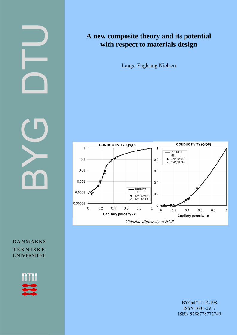
Chloride diffusivity of HCP.

CONDUCTIVITY (Q/QP)

0.00001

0.0001

0.001

0.01

0.1

1

0 0.2 0.4 0.6 0.8 1

Capillary porosity - c

PREDICTHSEXP(20%Si)EXP(6%Si)

CONDUCTIVITY (Q/QP)

0

0.2

0.4

0.6

0.8

1

0 0.2 0.4 0.6 0.8 1Capillary porosity - c

PREDICTHSEXP(20%Si)EXP(6% Si)

A new composite theory and its potential with respect to materials design

Lauge Fuglsang Nielsen

DANMARKS

T E K N I S K E UNIVERSITET

i

BYG•DTU R-198 ISSN 1601-2917

ISBN 9788778772749

A new composite theory and its potential with respect to materials design

Lauge Fuglsang Nielsen

Content 1. INTRODUCTION ............................................................................................................. 1

1.1 General conditions....................................................................................................... 2 1.2 Global composite properties ........................................................................................ 3

1.2.1 Bounds on stiffness and conductivity................................................................... 3 2. COMPOSITE GEOMETRY.............................................................................................. 4

2.1 An overview ................................................................................................................ 4 2.2 Classification of composites ........................................................................................ 5

2.2.1 Description of composite geometry ..................................................................... 7 2.2.2 Geo-path graph..................................................................................................... 7

2.3 Geo-parameters............................................................................................................ 8 2.3.1 Geo-path factor..................................................................................................... 8 2.3.2 Shape factors for particulate composites.............................................................. 8

Uni-shape mixture..................................................................................................... 9 Double-shape mixture............................................................................................... 9

2.3.3 Shape factors for laminar composites ................................................................ 10 2.3.4 Critical concentrations versus interaction .......................................................... 10

Interaction ............................................................................................................... 10 Critical concentration.............................................................................................. 10

2.3.5 Underlying geometry.......................................................................................... 11 3. PREPARATION OF COMPOSITE ANALYSIS............................................................ 11

3.1 Type of analysis......................................................................................................... 11 3.2 Shape- and geometry functions ................................................................................. 11

4. MATERIALS DESIGN ................................................................................................... 12 4.1 Geometry versus composite property ........................................................................ 13 4.2 Processing model ....................................................................................................... 13

4.2.1 Present work....................................................................................................... 14 5. PREDICTION AND DESIGN – illustrative examples ................................................... 14

5.1 Basic geometries........................................................................................................ 14 Analysis .................................................................................................................. 15 Discussion............................................................................................................... 15

5.2 Miscellaneous ............................................................................................................ 16 5.2.1 Stiffness and conductivity of porous material .................................................... 16

Analysis .................................................................................................................. 17 Discussion............................................................................................................... 17

5.2.2 Electrical conductivity of Binary Metallic mixture............................................ 17 Analysis .................................................................................................................. 18 Discussion – processing model............................................................................... 18

5.2.3 Stiffness of empty and impregnated HCP .......................................................... 18 Analysis .................................................................................................................. 19 Discussion............................................................................................................... 19

5.2.4 Chloride diffusivity of HCP ............................................................................... 19 Analysis .................................................................................................................. 20 Discussion – processing model............................................................................... 20

5.2.5 Alternative geometry.......................................................................................... 21 Discussion............................................................................................................... 22

ii

5.3 Application of underlying geometries ....................................................................... 22 5.3.1 Stiffness of a compacted powder composite ...................................................... 22

Analysis .................................................................................................................. 22 Discussion – processing model............................................................................... 23

5.3.2 Conductivity of composite with very long fibers ............................................... 23 Analysis .................................................................................................................. 23 Discussion............................................................................................................... 23

6. CONCLUSION AND FINAL REMARKS ..................................................................... 24 7. NOTATIONS................................................................................................................... 24

Appendix A: Shape factor for multi-shape mixture......................................................... 25 Appendix B: Underlying geometry ................................................................................. 26

Budiansky.................................................................................................................... 26 Stang............................................................................................................................ 27

Appendix C: Numerical determination of shape functions ............................................. 28 8. LITERATURE................................................................................................................. 28

iii

A new composite theory and its potential with respect to materials design

Lauge Fuglsang Nielsen∗)

Abstract: An operational summary of a new composite theory previously developed by the author is presented in this paper. ‘Global’ property solutions are presented which are valid for any composite geometry. Properties looked at are mechanical, such as stiffness, eigenstrain/stress (e.g. shrinkage and thermal expansion), and phy-sical, such as various conductivities with respect to heat, electricity, and diffusion. ‘Local’ property solutions applying for specific composites are obtained from the global solutions introducing geometry specific, so-called shape functions. The geometrical concept applied includes simple geometrical models (such as sphe-res, discs, and fibers) on which well-known composite theories from the literature are based. Examples are presented, demonstrating a very satisfying agreement be-tween material properties determined experimentally and such properties predicted by the theory considered. In a special section of this paper the theory is examined with respect to its potential with respect to materials design. Examples are presented, demonstrating how the pre-diction method can be inversed to determine types of composite geometry from pre-scribed composite properties, such as Young’s moduli and conductivities. A software (‘COMPREDES’) is prepared with application programs covering both the prediction aspects and the design aspects of the method presented. On request this software is available for the reader who has a special interest in the subjects con-sidered. Keywords: Composite materials, composite geometry, property prediction, design of geometry for prescribed properties.

1. INTRODUCTION The present paper is based on a composite theory for isotropic composite materials presented by the author in (1,2) by which ‘global’ solutions to composite problems can be determined for any composite, irrespective of geometry. ‘Local’ solutions ap-plying for composites with specific geometries are subsequently obtained from the global solutions introducing so-called shape functions.

Examples are presented in (1,2), demonstrating a very satisfying agreement between material properties determined experimentally and such properties predicted by the theory developed.

The geometrical concept applied includes simple geometrical models (such as sphe-res, discs, and fibers) on which well-known composite theories from the literature are based. This means that composite properties predicted by the author’s theory are consistent with such predicted by authors such as Hashin/Shtrikman (3,4), Hill (5), Maxwell (6), Böttcher/Landauer (7,8), and Budiansky (9). Furthermore, the theory is consistent with theories for special particulate composites (with ellipsoidal inclu-sions) such as developed by Christoffersen, Levin, and Stang (10,11,12).

The ‘global’ feature of the theory means that it has a potential with respect to mate-rials design. In order to study this potential more closely, an operational summary ∗) Dep. Civ. Eng., Tech. Uni. Denmark, dk-2800 Lyngby, Denmark - e-mail: lfn@byg.dtu.dk

1

of the author’s composite theory is presented in the first part of this article. Some studies on materials design are then presented in the second part.

Remark: It is not the purpose of the present paper to consider viscoelastic composi-tes. Readers especially interested in such materials are referred to (1,2) where the results presented in this paper are generalized to include viscoelastic composites.

1.1 General conditions The composites considered are isotropic mixtures of two components: phase P and phase S. The amount of phase P in phase S is quantified by the so-called volume con-centration defined by c = VP/(VP+VS) where volumes are denoted by V. In general, flexible phase geometries are considered which can adjust them selves to form a tight composite. The adjustment can be thought of as the result of a melting- or compaction process.

It is assumed that both phases exhibit linearity between response and gradient of po-tentials, which they are subjected to. For example: Mechanical stress versus deformati-on (Hooke's law), heat flow versus temperature, flow of electricity versus electric po-tential, and diffusion of a substance versus concentration of substance.

The composite properties specifically considered are stiffness, eigenstrain, and various conductivities as related to volume concentration, composite geometry, and phase pro-perties such as Young's moduli EP and ES (with stiffness ratio n = EP/ES), eigenstrains λP and λS, and conductivities QP and QS (with conductivity ratio nQ = QP/QS). Further notations used in the text are explained in the list of notations at the end of the paper.

In general the following assumptions are introduced:

- For simplicity (but also to reflect most composite problems encountered in practice) stiffness and stress results presented exhibit elastic phase behavior with Poisson’s rati-os ν = 0.2 (in practice ν ≈ 0.2). This means that, whenever stiffness and stress expres-sions are presented, they can be considered as generalized quantities, applying for any loading mode: shear, volumetric, as well as uni-axial. For example, E/ES can also be used to predict the composite shear modulus, G/GS, and the composite bulk modulus, K/KS, normalized with respect to the phase S properties. In a similar way the phase stresses1), σP/σ and σS/σ, also apply independently of loading mode as long as both phase stress modes (σP,σS) and composite (external) stress modes (σ) are the same.

- Not to exaggerate our present knowledge of composite geometries it has, delibe-rately, been chosen to keep geometry described by simple mathematical expres-sions.

Formally, the original theory in (1,2) is simplified very much by these assumptions: Only the volumetric analysis, for example, has to be considered - and the tensor no-tation can be dropped.

Remark: Composites, which do not comply immediately with these general condi-tions, can often be considered by easy modifications (1,2) of the theory presented. Examples are: particulate composites with non-flexible particles (causing self-in-flicted voids), incomplete phase contact, and incomplete impregnation.

1. As in (1,2), phase stress and phase strain are defined in this paper by their respective volume ave-rages in phase considered.

2

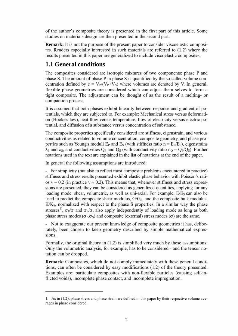
1.2 Global composite properties

Figure 1. The overall influence of phase P geometry on the geo-functions, θ, for stiffnessand, θQ, for conductivity. Phase P being spheres in a continuous phase S (CSAP) is definedby θ ≡ 1 and θQ ≡ 2 respectively. Phase S being spheres in a continuous phase P (CSAS) isdefined by θ ≡ n and θQ ≡ 2nQ respectively. Composites with geometries between these ex-tremes have θ and θQ in shaded areas.

As previously mentioned, the theory in (1,2) predicts global solutions for composite problems. Examples are presented in Equations 1 - 4 with symbols explained in the list of notations at the end of this paper. The influence of geometry on these solutions is ‘hidden’ in so-called geo-functions, θ and θQ, presented in Section 3.2 of this paper. The overall influence of geometry on these functions is illustrated in Figure 1.

Eigenstrain (linear)1/e - 1

λ = + ∆λ ; (∆λ = - )λ λ λS P S1/n - 1

Eigenstress (hydrostatic) (3)5 c(1/n - 1) - (1/e - 1) c

ρ = - E ∆λ ; ρ = - ρP PS S23 1 - cc(1/n - 1)

S tre s s d u e to e x te rn a l lo a d (σ )

n (1 + θ ) n + θσσ SP = ; = (2 )σ n + θ [1 + c (n - 1 )] σ n + θ [1 + c (n - 1 )]

)

( )

(

=

=S

PQ

S

E

Qn

Q

e = = nE n + θ - c ( n - 1 )S

C o n d u c t i v i t y : ( 1 ) + [ 1 + c ( - 1 ) ]n θ nQ Q Q Qq = =

+ - c ( - 1 )Q n θ nQ Q QS

PES t i f f n e s s :

n + θ [ 1 + c ( n - 1 ) ]E

Remark: Equations 2 and 3 are presented, mainly because of their significance with respect to composite design in general. They are not further considered in this paper because they are of no immediate interest for the main topics studied.

1.2.1 Bounds on stiffness and conductivity The above stiffness- and conductivity predictions are bounded as follows between the exact solutions for the CSA composites illustrated in Figures 2 and 3:

3

≤

≤

S t i f f n e s s - b o u n d sn + 1 + c ( n - 1 ) E 2 + c ( n - 1 )

e = < nn + 1 - c ( n - 1 ) 2 n - c ( n - 1 )E S

v a l i d f o r n > 1 ; r e v e r s e s i g n s w h e n n < 1( 4 )

C o n d u c t i v i t y - b o u n d s + 2 [ 1 + c ( - 1 ) ]n nQ Q q

+ 2 - c ( - 1 )n nQ Q

3 + 2 c ( - 1 )Q n Q= < n Q 3 - c ( - 1 )Q n nQ QSv a l i d f o r > 1 ; r e v e r s e s i g n s w h e n < 1n nQ Q

The stiffness bounds are obtained from Equation 1 introducing θ ≡ 1 and θ ≡ n re-spectively. The conductivity bounds are obtained introducing θQ ≡ 2 and θQ ≡ 2nQ respectively. The bounds such determined are the same as can be obtained from the studies made by Hashin and Shtrikman in (3) on composite stiffness and in (4) on composite conductivity. The left side conductivity expression in Equation 4 equals the well-known Maxwell relation (6) for electrical and magnetic permeability of particulate composites with spherical particles. The Hashin/Shtrikman’s bounds are subsequently referred to by H/S.

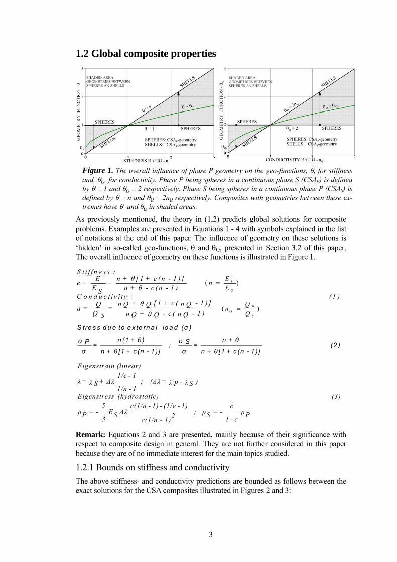
Remarks: We notice in this context that the composite theory developed in (1,2) is based on the concept that any isotropic composite geometry is a station on a geo-path moving from the CSAP geometry shown in Figure 2 to the CSAS geometry shown in Figure 3. (CSA is an abbreviation for the composite model, Composite Spheres Assemblage, introduced by Hashin in (13)). It is emphasized that the phase numbering P, S, throughout the paper, keeps consistent with this geometrical con-cept.

Figure 3. Composite Spheres Assemblagewith phase S particles, CSAS.

Figure 2. Composite Spheres Assemblagewith phase P particles, CSAP.

2. COMPOSITE GEOMETRY 2.1 An overview Geometries in a composite changes as the result of volume transformations associated with increasing phase P concentration. We will think of changes as they are stylized in Figure 4: At increasing concentration, from c = 0, discrete phase P elements agglome-rate and change their shapes approaching a state at the so-called critical concentration, cS, where they start forming continuous geometries. Phase P grows fully continuous between cS and the second critical concentration, cP > cS, such that the composite geo-metry from the latter concentration has become a mixture of discrete, de-agglomera-ting, phase S particles in a continuous phase P.

4

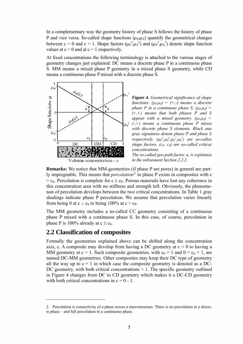
In a complementary way the geometry history of phase S follows the history of phase P and vice versa. So-called shape functions (µP,µS) quantify the geometrical changes between c = 0 and c = 1. Shape factors (µP

o,µSo) and (µP

1,µS1) denote shape function

values at c = 0 and at c = 1 respectively.

At fixed concentrations the following terminology is attached to the various stages of geometry changes just explained: DC means a discrete phase P in a continuous phase S. MM means a mixed phase P geometry in a mixed phase S geometry, while CD means a continuous phase P mixed with a discrete phase S.

Figure 4. Geometrical significance of shapefunctions: (µP,µS) = (+,-) means a discretephase P in a continuous phase S. (µP,µS) =(+,+) means that both phases P and Sappear with a mixed geometry. (µP,µS) =(-,+) means a continuous phase P mixedwith discrete phase S elements. Black andgray signatures denote phase P and phase Srespectively. (µP

o,µSo,µP

1,µS1) are so-called

shape factors, (cP, cS) are so-called criticalconcentrations. The so-called geo-path factor, a, is explainedin the subsequent Section 2.2.2.

Remarks: We notice that MM-geometries (if phase P are pores) in general are part-ly impregnable. This means that percolation2) in phase P exists in composites with c > cS. Percolation is complete for c ≥ cP. Porous materials have lost any coherence in this concentration area with no stiffness and strength left. Obviously, the phenome-non of percolation develops between the two critical concentrations. In Table 1 gray shadings indicate phase P percolation. We assume that percolation varies linearly from being 0 at c # cS to being 100% at c > cP.

The MM geometry includes a so-called CC geometry consisting of a continuous phase P mixed with a continuous phase S. In this case, of course, percolation in phase P is 100% already at c ≥ cS.

2.2 Classification of composites Formally the geometries explained above can be shifted along the concentration axis, c. A composite may develop from having a DC geometry at c = 0 to having a MM geometry at c = 1. Such composite geometries, with cP > 1 and 0 < cS < 1, are named DC-MM geometries. Other composites may keep their DC type of geometry all the way up to c = 1 in which case the composite geometry is denoted as a DC-DC geometry, with both critical concentrations > 1. The specific geometry outlined in Figure 4 changes from DC to CD geometry which makes it a DC-CD geometry with both critical concentrations in c = 0 - 1.

2. Percolation is connectivity of a phase across a microstructure. There is no percolation in a discre-te phase – and full percolation in a continuous phase.

5

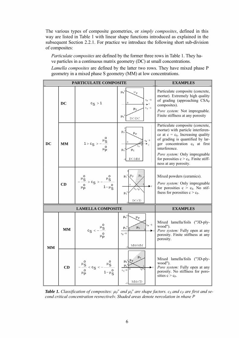
The various types of composite geometries, or simply composites, defined in this way are listed in Table 1 with linear shape functions introduced as explained in the subsequent Section 2.2.1. For practice we introduce the following short sub-division of composites:

Particulate composites are defined by the former three rows in Table 1. They ha-ve particles in a continuous matrix geometry (DC) at small concentrations. Lamella composites are defined by the latter two rows. They have mixed phase P geometry in a mixed phase S geometry (MM) at low concentrations.

PARTICULATE COMPOSITE EXAMPLES

DC c 1S >

Particulate composite (concrete, mortar). Extremely high quality of grading (approaching CSAP composites). Pore system: Not impregnable. Finite stiffness at any porosity

MM oS1 cS oP

µ> > −

µ

Particulate composite (concrete, mortar) with particle interferen-ce at c = cS. Increasing quality of grading is quantified by lar-ger concentration cS at first interference. Pore system: Only impregnable for porosities c > cS. Finite stiff-ness at any porosity.

DC

CD

o oS ScSo o1P S

µ µ− > > −

µ − µ

Mixed powders (ceramics).

Pore system: Only impregnable for porosities c > cS. No stif-fness for porosities c > cP.

LAMELLA COMPOSITE EXAMPLES

MM oScS oP

µ< −

µ

Mixed lamella/foils ("3D-ply-wood"). Pore system: Fully open at any porosity. Finite stiffness at any porosity.

MM

CD o oS ScSo o1P S

µ µ− < < −

µ − µ

Mixed lamella/foils ("3D-ply-wood"). Pore system: Fully open at any porosity. No stiffness for poro-sities c > cP.

Table 1. Classification of composites: µPo and µS

o are shape factors. cS and cP are first and se-cond critical concentration respectively. Shaded areas denote percolation in phase P

6

Remarks: We notice that critical concentrations can be fictitious (outside c = 0 - 1). In such cases they do not, of course, have the immediate physical meanings previ-ously indicated. Formally, however, we do keep these meanings in order to describe in an easy way, how composite geometry changes with phase concentrations – and how ‘fast’ phase elements interact with each other (interaction increases with slopes of shape functions).

2.2.1 Description of composite geometry As recommended in Section 1.1, simple mathematical expressions are preferred for the description of composite geometry. As such we chose from (1,2) the simple rela-tion in Equation 5 which considers shape functions to vary linearly with phase P con-centrations with cS, µP

o, and µSo as independent variables3).

( ) ( ) / (= −≤ ≤ ≤ ≤

c co o o o = µ 1 - ; = µ 1 - with c c shape functions) (5)µ µ P SP SP PS Sc cP STruncate to hold - 1 µ 1 and - 1 µ 1P S

µ µ

Implicitly this expression means that types of composite geometries are considered to be phase-symmetric with respect to cSYM = (cP + cS)/2. Meaning that the phase P/S shape function at c = cSYM - ∆c is similar to the phase S/P shape function at c = cSYM + ∆c. (The statement of phase-symmetry applies only ‘inside’ the truncated parts of the shape functions).

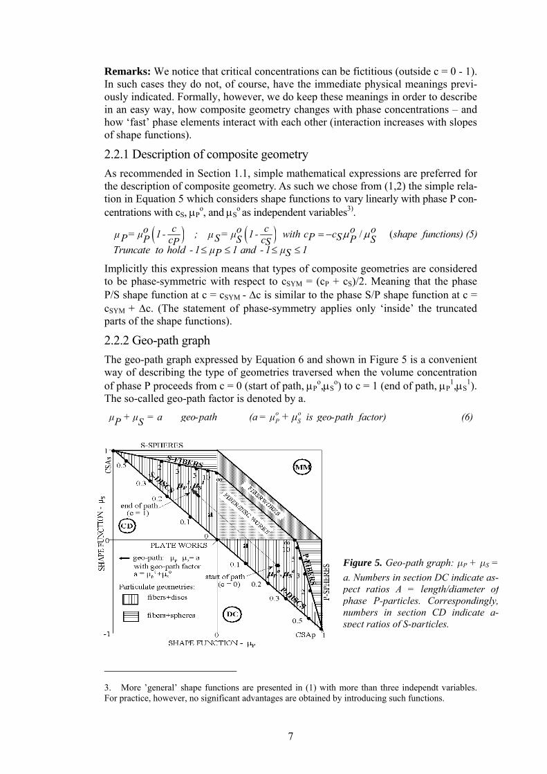
2.2.2 Geo-path graph The geo-path graph expressed by Equation 6 and shown in Figure 5 is a convenient way of describing the type of geometries traversed when the volume concentration of phase P proceeds from c = 0 (start of path, µP

o,µSo) to c = 1 (end of path, µP

1,µS1).

The so-called geo-path factor is denoted by a. o oP Sµ + µ = a geo-path (a = µ is geo-path factor) (6)+ µ

P S

Figure 5. Geo-pat = a. Numbers in sect

h graph: µP + µS

ion DC indicate as-pect ratios A = length/diameter o

3. More ’general’ shape functions are presented in (1) with more than three independt variables. For practice, however, no significant advantages are obtained by introducing such functions.

f phase P-particnumbers in sec

les. C ngly, tio e a-

orrespondin CD indicat

spect ratios of S-particles.

7

The numbers in Figure 5 refer to shape factors for composites ma

, ≤ ≤≥

The geo-path- factor 0 a 1, increases with length of phase componentsoParticulate composites have shape factors µ a (7)PoLaminar composites have shape factors µ < aP

de with uni-sha-

he requirement of shape d in Equation 5 ensures that the basic geometrical con- kept: Every phase geometry considered is a station on

rameters will be discussed more closely - for example with respect to the possibility of determining them for practice.

2.3.1 Geo-path factor

ped particles with aspect ratios (see figure legend) as indicated. Shaded areas refer to shape factors for multi-shaped mixtures defined in the figure. In details shape factors are considered in the subsequent Section 2.3.

We notice that geo-paths orientated according to Figure 5 means that the shape function µP decreases with c while µS increases with c. Tfunction truncation introducecept previously introduced isa path going from a CSAP geometry to a CSAS geometry.

2.3 Geo-parameters In this section the geo-pa

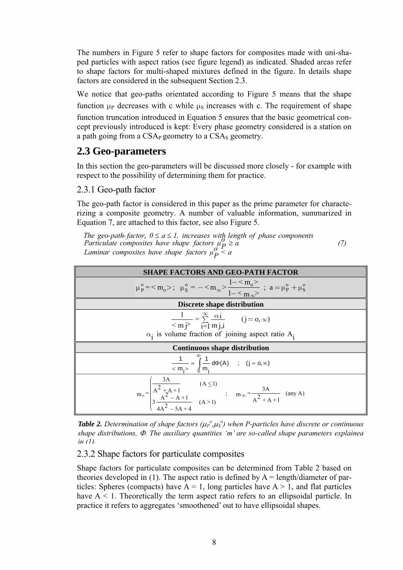
The geo-path factor is considered in this paper as the prime parameter for characte-rizing a composite geometry. A number of valuable information, summarized in Equation 7, are attached to this factor, see also Figure 5.

SHAPE FACTORS AND GEO-PATH FACTOR

o o o ooo P SP S

1 < m > = < m ; = < m > ; a

1 < >m∞∞

−> − =µ +µµ µ

−

Discrete shape distribution 1 i = ( j o, )

> < m mj j,ii=1is volume fraction of joining aspect ratio Ai i

∞∞α =∑

α

Continuous shape distribution

0j j

1 1d (A) ; ( j o, )

m m

∞= Φ =

< > ∫ ∞

o

3A(A 1)≤2 3AA + A + 1 = ; = (any A)m m2 2A A + 1 A + A 13 (A > 1)24A 5A + 4

∞−

−

⎛⎜⎜⎜⎜⎜⎜⎜⎜⎜⎜⎝

+

Table 2. Determination of shape factors (µPo,µS

o) when P-particles have discrete or continuousshape distributions, Φ. The auxiliary quantities ‘m’ are so-called shape parameters explained in (1).

2.3.2 Shape factors for particulate composites

In practice it refers to aggregates ‘smoothened’ out to have ellipsoidal shapes.

Shape factors for particulate composites can be determined from Table 2 based on theories developed in (1). The aspect ratio is defined by A = length/diameter of par-ticles: Spheres (compacts) have A = 1, long particles have A > 1, and flat particles have A < 1. Theoretically the term aspect ratio refers to an ellipsoidal particle.

8

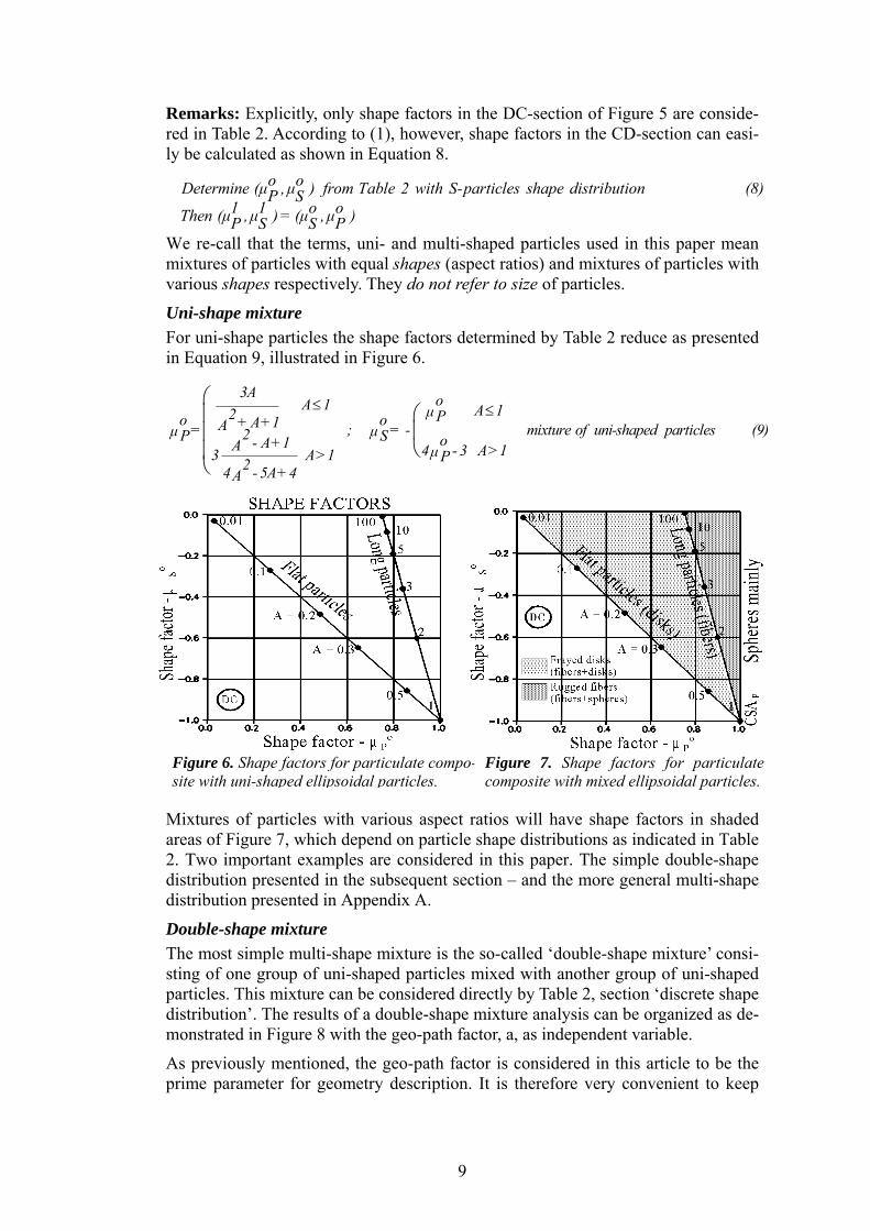
Remarks: Explicitly, only shape factors in the DC-section of Figure 5 are conside-red in Table 2. According to (1), however, shape factors in the CD-section can easi-ly be calculated as shown in Equation 8.

o oDetermine (µ ,µ ) from Table 2 with S-particles shape distribution (8)P S1 1 o oThen (µ ,µ ) = (µ ,µ )P PS S

We re-call that the terms, uni- and multi-shaped particles used in this paper mean mixtures of particles with equal shapes (aspect ratios) and mixtures of particles with various shapes respectively. They do not refer to size of particles.

Uni-shape mixture

≤ ≤⎛

⎛⎜⎜⎜⎝⎜

⎝

3A o A 1 A 1µ2 Po o + A + 1A = ; = - mixture of uni-shaped particles (9)µ µ2P S o - A + 1A 4 - 3 A > 1µ3 A > 1 P24 - 5A + 4A

9

Figure 6. Shape factors for particulate compo-site with uni-shaped ellipsoidal particles.

Figure 7. Shape factors for particulatecomposite with mixed ellipsoidal particles.

For uni-shape particles the shape factors determined by Table 2 reduce as presented

Mixtures of particles with various as

in Equation 9, illustrated in Figure 6.

pect ratios will have shape factors in shaded

hape mixture is the so-called ‘double-shape mixture’ consi-

o be the

areas of Figure 7, which depend on particle shape distributions as indicated in Table 2. Two important examples are considered in this paper. The simple double-shape distribution presented in the subsequent section – and the more general multi-shape distribution presented in Appendix A.

Double-shape mixture The most simple multi-ssting of one group of uni-shaped particles mixed with another group of uni-shaped particles. This mixture can be considered directly by Table 2, section ‘discrete shape distribution’. The results of a double-shape mixture analysis can be organized as de-monstrated in Figure 8 with the geo-path factor, a, as independent variable.

As previously mentioned, the geo-path factor is considered in this article tprime parameter for geometry description. It is therefore very convenient to keep

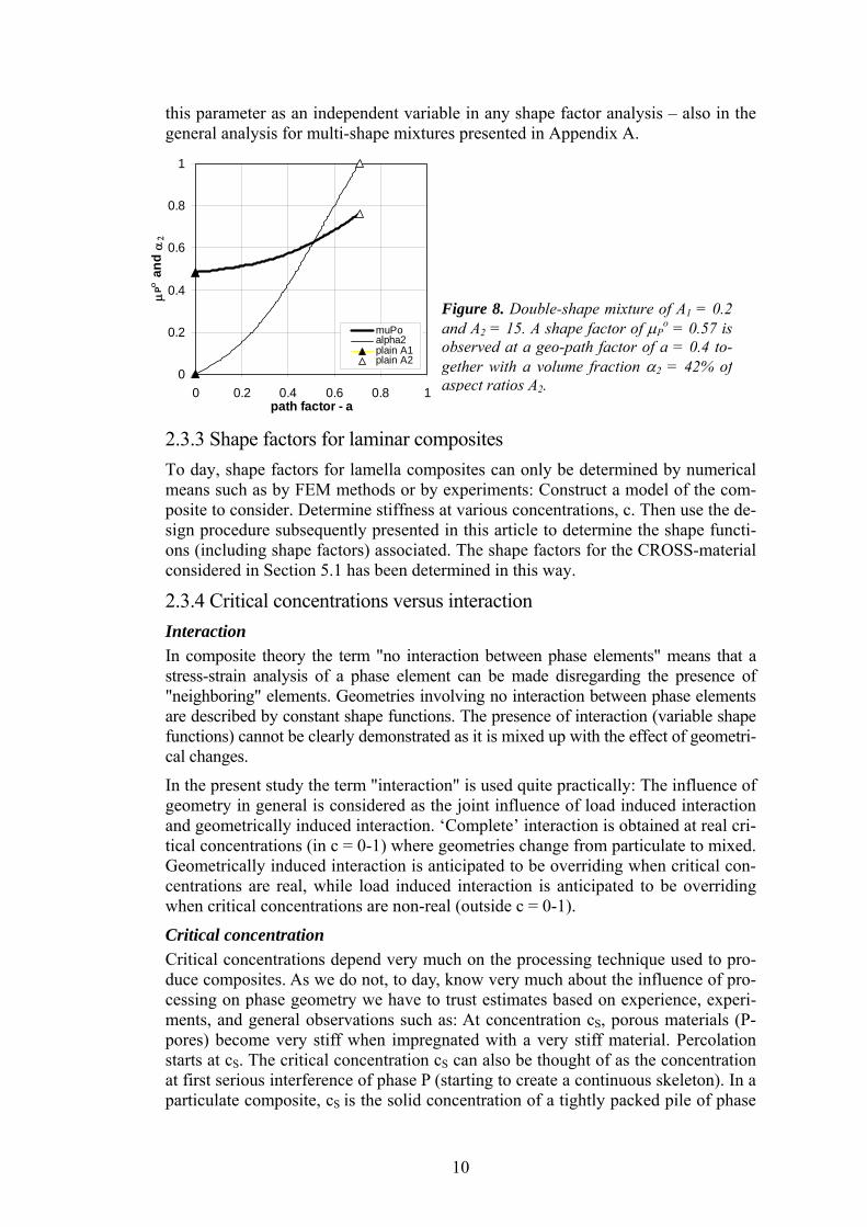
this parameter as an independent variable in any shape factor analysis – also in the general analysis for multi-shape mixtures presented in Appendix A.

10

0

0.2

0.4

0.6

0.8

1

0 0.2 0.4 0.6 0.8 1path factor - a

µPο

and

α2

muPoalpha2plain A1plain A2

Figure 8. Double-shape mixture of A1 = 0.2 and A2 = 15. A shape factor of µP

o = 0.57 is observed at a geo-path factor of a = 0.4 to-gether with a volume fraction α2 = 42% of aspect ratios A2.

2.3.3 Shape factors for laminar composites To day, shape factors for lamella composites can only be determined by numerical means such as by FEM methods or by experiments: Construct a model of the com-posite to consider. Determine stiffness at various concentrations, c. Then use the de-sign procedure subsequently presented in this article to determine the shape functi-ons (including shape factors) associated. The shape factors for the CROSS-material considered in Section 5.1 has been determined in this way.

2.3.4 Critical concentrations versus interaction Interaction In composite theory the term "no interaction between phase elements" means that a stress-strain analysis of a phase element can be made disregarding the presence of "neighboring" elements. Geometries involving no interaction between phase elements are described by constant shape functions. The presence of interaction (variable shape functions) cannot be clearly demonstrated as it is mixed up with the effect of geometri-cal changes.

In the present study the term "interaction" is used quite practically: The influence of geometry in general is considered as the joint influence of load induced interaction and geometrically induced interaction. ‘Complete’ interaction is obtained at real cri-tical concentrations (in c = 0-1) where geometries change from particulate to mixed. Geometrically induced interaction is anticipated to be overriding when critical con-centrations are real, while load induced interaction is anticipated to be overriding when critical concentrations are non-real (outside c = 0-1).

Critical concentration Critical concentrations depend very much on the processing technique used to pro-duce composites. As we do not, to day, know very much about the influence of pro-cessing on phase geometry we have to trust estimates based on experience, experi-ments, and general observations such as: At concentration cS, porous materials (P-pores) become very stiff when impregnated with a very stiff material. Percolation starts at cS. The critical concentration cS can also be thought of as the concentration at first serious interference of phase P (starting to create a continuous skeleton). In a particulate composite, cS is the solid concentration of a tightly packed pile of phase

P particles. Obviously, critical concentrations in particulate composites are closely related to particles size distributions.

At the second critical concentration, cP > cS, the composite phase S elements beco-me completely wrapped in a matrix of phase P. Porous materials loose their stiffness and strength at cP because phase P has become a continuous, enveloping, void sy-stem.

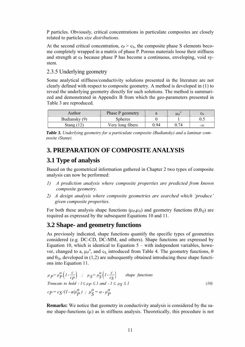
2.3.5 Underlying geometry Some analytical stiffness/conductivity solutions presented in the literature are not clearly defined with respect to composite geometry. A method is developed in (1) to reveal the underlying geometry directly for such solutions. The method is summari-zed and demonstrated in Appendix B from which the geo-parameters presented in Table 3 are reproduced.

Author Phase P geometry a µPo cS

Budiansky (9) Spheres 0 1 0.5

Stang (12) Very long fibers 0.94 0.74 -∞

Table 3. Underlying geometry for a particulate composite (Budiansky) and a laminar com-posite (Stang).

3. PREPARATION OF COMPOSITE ANALYSIS 3.1 Type of analysis Based on the geometrical information gathered in Chapter 2 two types of composite analysis can now be performed:

1) A prediction analysis where composite properties are predicted from known composite geometry.

2) A design analysis where composite geometries are searched which ‘produce’ given composite properties.

For both these analysis shape functions (µP,µS) and geometry functions (θ,θQ) are required as expressed by the subsequent Equations 10 and 11.

3.2 Shape- and geometry functions As previously indicated, shape functions quantify the specific types of geometries considered (e.g. DC-CD, DC-MM, and others). Shape functions are expressed by Equation 10, which is identical to Equation 5 – with independent variables, howe-ver, changed to a, µP

o, and cS, introduced from Table 4. The geometry functions, θ and θQ, developed in (1,2) are subsequently obtained introducing these shape functi-ons into Equation 11.

( ) ( )≤ ≤≤ ≤

c co o = µ 1 - ; = µ 1 - shape functionsµ µP SP Sc cP STruncate to hold - 1 µ 1 and - 1 µ 1 (10)P S

c o o o= c /(1 - a/µ ) ; µ = a - µP S P PS

Remarks: We notice that geometry in conductivity analysis is considered by the sa-me shape-functions (µ) as in stiffness analysis. Theoretically, this procedure is not

11

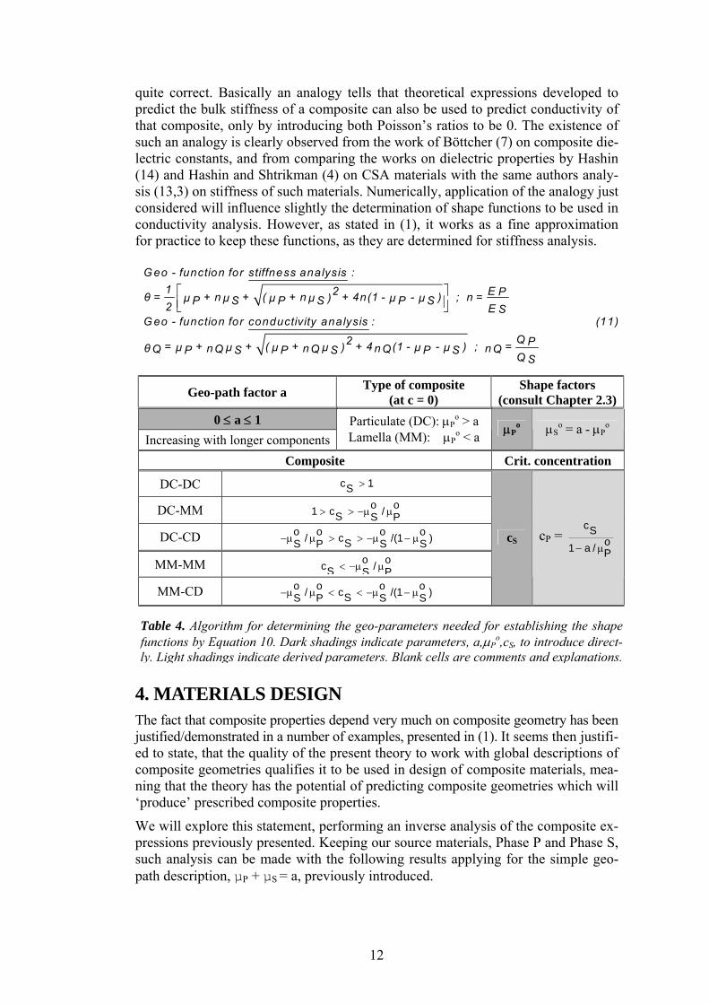
quite correct. Basically an analogy tells that theoretical expressions developed to predict the bulk stiffness of a composite can also be used to predict conductivity of that composite, only by introducing both Poisson’s ratios to be 0. The existence of such an analogy is clearly observed from the work of Böttcher (7) on composite die-lectric constants, and from comparing the works on dielectric properties by Hashin (14) and Hashin and Shtrikman (4) on CSA materials with the same authors analy-sis (13,3) on stiffness of such materials. Numerically, application of the analogy just considered will influence slightly the determination of shape functions to be used in conductivity analysis. However, as stated in (1), it works as a fine approximation for practice to keep these functions, as they are determined for stiffness analysis.

⎡ ⎤⎢ ⎥⎣ ⎦

G eo - function for stiffness analysis :1 E2 Pθ = + n + ( + n + 4n(1 - - ) ; n = µ µ µ µ ) µ µP S P S P S2 E S

G eo - function for conductivity analysis : (11)

2 = + + ( + + 4 (1 - - ) ; µ µ µ µ ) µ µθ n n nQ Q Q QQ P S P S P SQ P = nQ S

Geo-path factor a Type of composite (at c = 0)

Shape factors (consult Chapter 2.3)

0 ≤ a ≤ 1 Increasing with longer components

Particulate (DC): µPo > a

Lamella (MM): µPo < a µP

o µSo = a - µP

o

Composite Crit. concentration

DC-DC c 1S >

DC-MM o o1 c /S S P> > −µ µ

DC-CD o o o o/ c /(1SS P S S−µ µ > > −µ − µ )

MM-MM o oc /S S P< −µ µ

MM-CD o o o o/ c /(1−µ µ < < −µ − µ )

cS cP = cS

o1 a / P− µ

SS P S S

Table 4. Algorithm for determining the geo-parameters needed for establishing the shapefunctions by Equation 10. Dark shadings indicate parameters, a,µP

o,cS, to introduce direct-ly. Light shadings indicate derived parameters. Blank cells are comments and explanations.

4. MATERIALS DESIGN The fact that composite properties depend very much on composite geometry has been justified/demonstrated in a number of examples, presented in (1). It seems then justifi-ed to state, that the quality of the present theory to work with global descriptions of composite geometries qualifies it to be used in design of composite materials, mea-ning that the theory has the potential of predicting composite geometries which will ‘produce’ prescribed composite properties.

We will explore this statement, performing an inverse analysis of the composite ex-pressions previously presented. Keeping our source materials, Phase P and Phase S, such analysis can be made with the following results applying for the simple geo-path description, µP + µS = a, previously introduced.

12

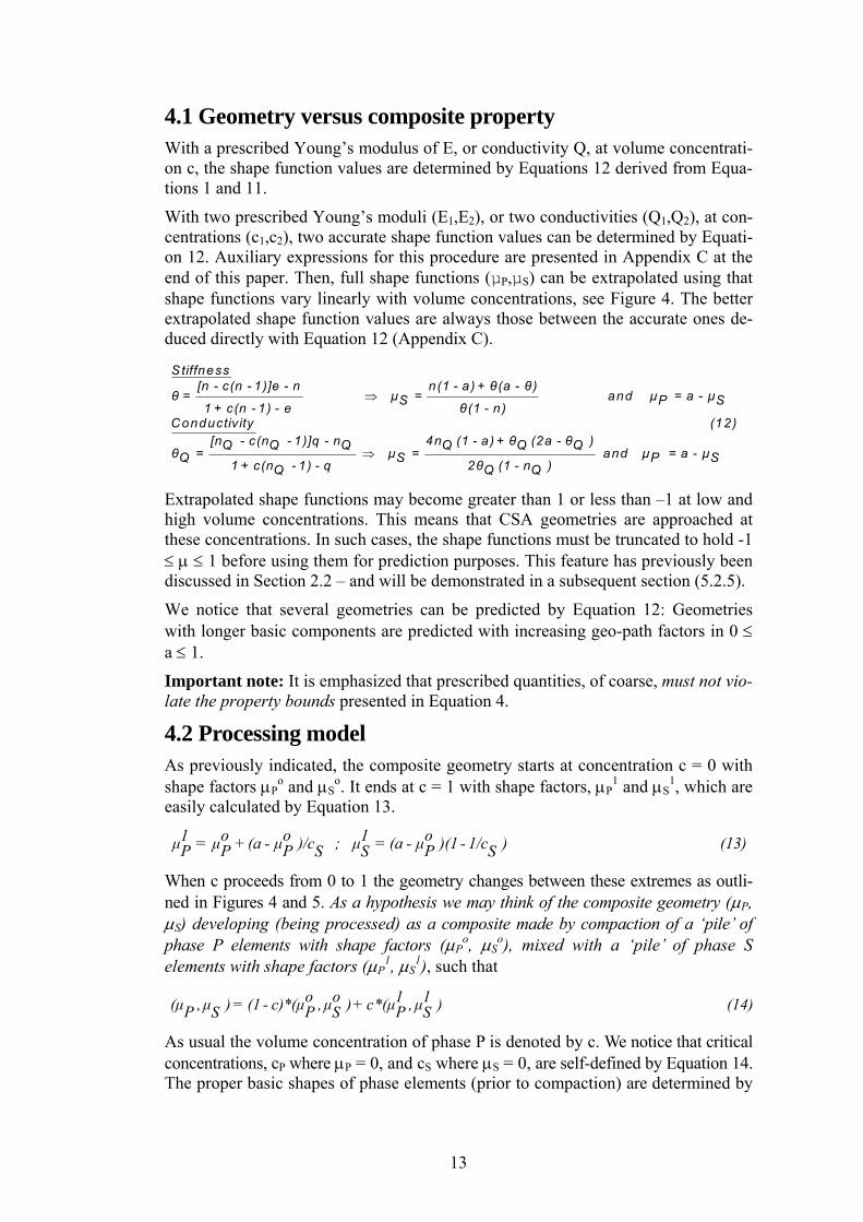
4.1 Geometry versus composite property With a prescribed Young’s modulus of E, or conductivity Q, at volume concentrati-on c, the shape function values are determined by Equations 12 derived from Equa-tions 1 and 11.

With two prescribed Young’s moduli (E1,E2), or two conductivities (Q1,Q2), at con-centrations (c1,c2), two accurate shape function values can be determined by Equati-on 12. Auxiliary expressions for this procedure are presented in Appendix C at the end of this paper. Then, full shape functions (µP,µS) can be extrapolated using that shape functions vary linearly with volume concentrations, see Figure 4. The better extrapolated shape function values are always those between the accurate ones de-duced directly with Equation 12 (Appendix C).

⇒

⇒

Stiffness[n - c(n - 1)]e - n n(1 - a) + θ (a - θ )

θ = µ = and µ = a - µS P1 + c(n - 1) - e θ (1 - n)Conductiv ity (12)

[n - c(n - 1)]q - n 4n (1 - a) + θ (2a - θ )Q Q Q Q Q Qθ = µ = anQ S1 + c(n - 1) - q 2θ (1 - n )Q Q Qd µ = a - µP S

S

Extrapolated shape functions may become greater than 1 or less than –1 at low and high volume concentrations. This means that CSA geometries are approached at these concentrations. In such cases, the shape functions must be truncated to hold -1 ≤ µ ≤ 1 before using them for prediction purposes. This feature has previously been discussed in Section 2.2 – and will be demonstrated in a subsequent section (5.2.5).

We notice that several geometries can be predicted by Equation 12: Geometries with longer basic components are predicted with increasing geo-path factors in 0 ≤ a ≤ 1.

Important note: It is emphasized that prescribed quantities, of coarse, must not vio-late the property bounds presented in Equation 4.

4.2 Processing model As previously indicated, the composite geometry starts at concentration c = 0 with shape factors µP

o and µSo. It ends at c = 1 with shape factors, µP

1 and µS1, which are

easily calculated by Equation 13. 1 o o 1 oµ = µ +(a - µ )/c ; µ = (a - µ )(1 - 1/c ) (13)P P P PS S S

When c proceeds from 0 to 1 the geometry changes between these extremes as outli-ned in Figures 4 and 5. As a hypothesis we may think of the composite geometry (µP, µS) developing (being processed) as a composite made by compaction of a ‘pile’ of phase P elements with shape factors (µP

o, µSo), mixed with a ‘pile’ of phase S

elements with shape factors (µP1, µS

1), such that

o o 1 1(µ , µ ) = (1 - c)*(µ , µ )+ c*(µ , µ ) (14)P P PS S S As usual the volume concentration of phase P is denoted by c. We notice that critical concentrations, cP where µP = 0, and cS where µS = 0, are self-defined by Equation 14. The proper basic shapes of phase elements (prior to compaction) are determined by

13

an inverse shape factor analysis (such as aspect ratios as a function of shape fac-tors).

Remarks: We re-call that (µPo, µS

o) quantifies the geometry of a dilute suspension of phase P. With no interaction between phase P-elements the composite geometry (µP, µS) stays at (µP

o, µSo). With interaction between phase P-elements, (µP, µS) varies with

concentration, c.

The processing model explained is consistent with a geometrical model implicitly used by Budiansky (9) in his classical analysis of composites made of phase P spheres mix-ed with phase S spheres. The composite geometry in the Budiansky analysis is presen-ted in Figure B1 (Appendix B).

4.2.1 Present work It is obvious from Section 2.3 that processing models can only be suggested for DC-CD composites4). An accurate inverse shape factor analysis cannot, presently, be per-formed in the MM section of Figure 5. Only tentative/inaccurate answers can be given to the question: Which mixed geometry is associated with known shape factors in the MM section? More research is needed in this area (see Section 2.3.3).

Because of this lack of generality only theoretical composite geometries are presen-ted in the ‘illustrative’ examples shown in the following Section 5. Exceptions are DC-CD composites where the conductivity of binary metallic mixtures, chloride diffusitivity of HCP, and stiffness of powder composites, respectively are conside-red.

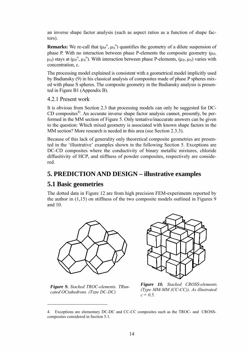
5. PREDICTION AND DESIGN – illustrative examples 5.1 Basic geometries The dotted data in Figure 12 are from high precision FEM-experiments reported by the author in (1,15) on stiffness of the two composite models outlined in Figures 9 and 10.

Figure 10. Stacked CROSS-elements.(Type MM-MM (CC-CC)). As illustrated:c = 0.5.

Figure 9. Stacked TROC-elements. TRun-cated OCtahedrons. (Type DC-DC)

4. Exceptions are elementary DC-DC and CC-CC composites such as the TROC- and CROSS-composites considered in Section 5.1.

14

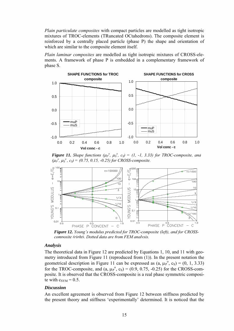
Plain particulate composites with compact particles are modelled as tight isotropic mixtures of TROC-elements (TRuncated OCtahedrons). The composite element is reinforced by a centrally placed particle (phase P) the shape and orientation of which are similar to the composite element itself.

Plain laminar composites are modelled as tight isotropic mixtures of CROSS-ele-ments. A framework of phase P is embedded in a complementary framework of phase S.

Figure 11. Shape functions (µPo, µS

o, cS) = (1, -1, 3.33) for TROC-composite, and(µP

o, µSo , cS) = (0.75, 0.15, -0.25) for CROSS-composite.

SHAPE FUNCTIONS for CROSS composite

-1.0

-0.5

0.0

0.5

1.0

0.0 0.2 0.4 0.6 0.8 1.0Vol conc - c

muPmuS

SHAPE FUNCTIONS for TROC composite

-1.0

-0.5

0.0

0.5

1.0

0.0 0.2 0.4 0.6 0.8 1.0Vol conc - c

muPmuS

Figure 12. Young’s modulus predicted for TROC-composite (left), and for CROSS-composite (right). Dotted data are from FEM analysis.

Analysis The theoretical data in Figure 12 are predicted by Equations 1, 10, and 11 with geo-metry introduced from Figure 11 (reproduced from (1)). In the present notation the geometrical description in Figure 11 can be expressed as (a, µP

o, cS) = (0, 1, 3.33) for the TROC-composite, and (a, µP

o, cS) = (0.9, 0.75, -0.25) for the CROSS-com-posite. It is observed that the CROSS-composite is a real phase symmetric composi-te with cSYM = 0.5.

Discussion An excellent agreement is observed from Figure 12 between stiffness predicted by the present theory and stiffness ‘experimentally’ determined. It is noticed that the

15

geo-parameters applied are consistent with the parameters presented in Table 5, which is based on Table 4.

We notice that the CROSS-composite has a shape factor of µPo = 0.75, which is the

same as for materials reinforced with very long fibers, see Figure 6. We also notice that the TROC-composite is very close to having a CSAP geometry (µP = -µS = 1).

Table 5. Geo-parameters for TROC and CROSS as estimated from Table 4.

Composite particle length a µPo cS

TROC (DC-DC) short (A ≈ 1, sphere) low 1 >1 CROSS (MM-MM) long (A ≈ ∞, fiber) high 0.75 <-µS

o/µPo = 1-a/µP

o

5.2 Miscellaneous In this section we will evaluate both the prediction- and design methods presented. We do that by considering experimental data sets known from the literature. From each data set we choose (or interpolate) two sets of concentration versus property data to represent ‘prescribed’ data. Then we use Section 4.1 to design which com-posite geometry can ‘produce’ these data.

For these geometries we then predict composite properties by the global solutions presented in Section 1.2 with shape- and geo-functions introduced as explained in Section 3.2. The quality of predicted data to coincide with the rest of the experimen-tal data considered is a reasonable success criterion for a good description of the composite geometry of the test material – and for the reliability of the total compo-site theory presented in this paper.

Remark: For reasons previously indicated in Section 4.2.1 processing models will only be considered in Sections 5.2.2, 5.2.4, and 5.3.1 where the conductivity of bi-nary metallic mixtures, chloride diffusitivity of HCP, and stiffness of powder com-posites respectively are the subjects of analysis.

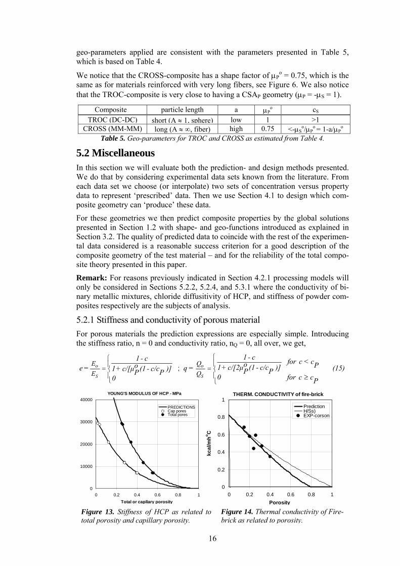
5.2.1 Stiffness and conductivity of porous material For porous materials the prediction expressions are especially simple. Introducing the stiffness ratio, n = 0 and conductivity ratio, nQ = 0, all over, we get,

;

⎧⎧⎪⎪= =⎨ ⎨

⎪ ⎪⎩ ⎩

≥S S

o oE QE Q

1 - c1 - c for c < co Po 1+ c/[2µ (1 - c/c )]e = q = (15)1+ c/[µ (1 - c/c )] P PP P 0 for c c0 P

Figure 13. Stiffness of HCP as related to total porosity and capillary porosity.

YOUNG'S MODULUS OF HCP - MPa

0

10000

20000

30000

40000

0 0.2 0.4 0.6 0.8 1Total or capllary porosity

PREDICTIONSCap poresTotal pores

THERM. CONDUCTIVITY of fire-brick

0

0.2

0.4

0.6

0.8

1

0 0.2 0.4 0.6 0.8 1Porosity

kcal

/mho C

PredictionH/Ss)EXP-corson

Figure 14. Thermal conductivity of Fire-brick as related to porosity.

16

It is noticed that only the geo-parameters µPo and cP are needed to predict stiff-

ness/conductivity of porous materials.

Remark: In this paper the term ’porous material’ also applies to composite materi-als where phase P has no conductivity, meaning that the conductivity ratio is nQ = 0.

The experimental data in Figure 13 on stiffness of hardened cement paste (HCP) are reported by Helmuth and Turk in (16, cement 15366). The experimental data in Fi-gure 14 on thermal conductivity of firebrick are reported by Corson in (17).

Analysis Equation 15 predicts the theoretical data in Figures 13 and 14 with the following material- and geo-parameters deduced in (1).

Solid is gel including gel pores: ES = 32000 MPa, µPo = 0.40, cP = 1.

Solid is plain (bulk) gel solid: ES = 80000 MPa, µPo = 0.33, cP = 1.

Solid is fired clay: QS = 0.825 kcal/mhoC, µPo = 1.0, cP = 0.82

Discussion The geo-parameters just presented are not sufficient to perform a general property analysis of the materials considered, such as the influence of impregnation on these materials. Table 4 can be used to determine the parameters needed. The results are presented in Table 6 with estimated geo-path factors.

Material a µPo cS

HCP: Cap-pores 0.3 0.4 0.25 HCP: Tot-pores 0.3 0.33 0.09

Firebrick 0.4 1 0.49

Table 6. Complete geometry of HCP and firebrick.

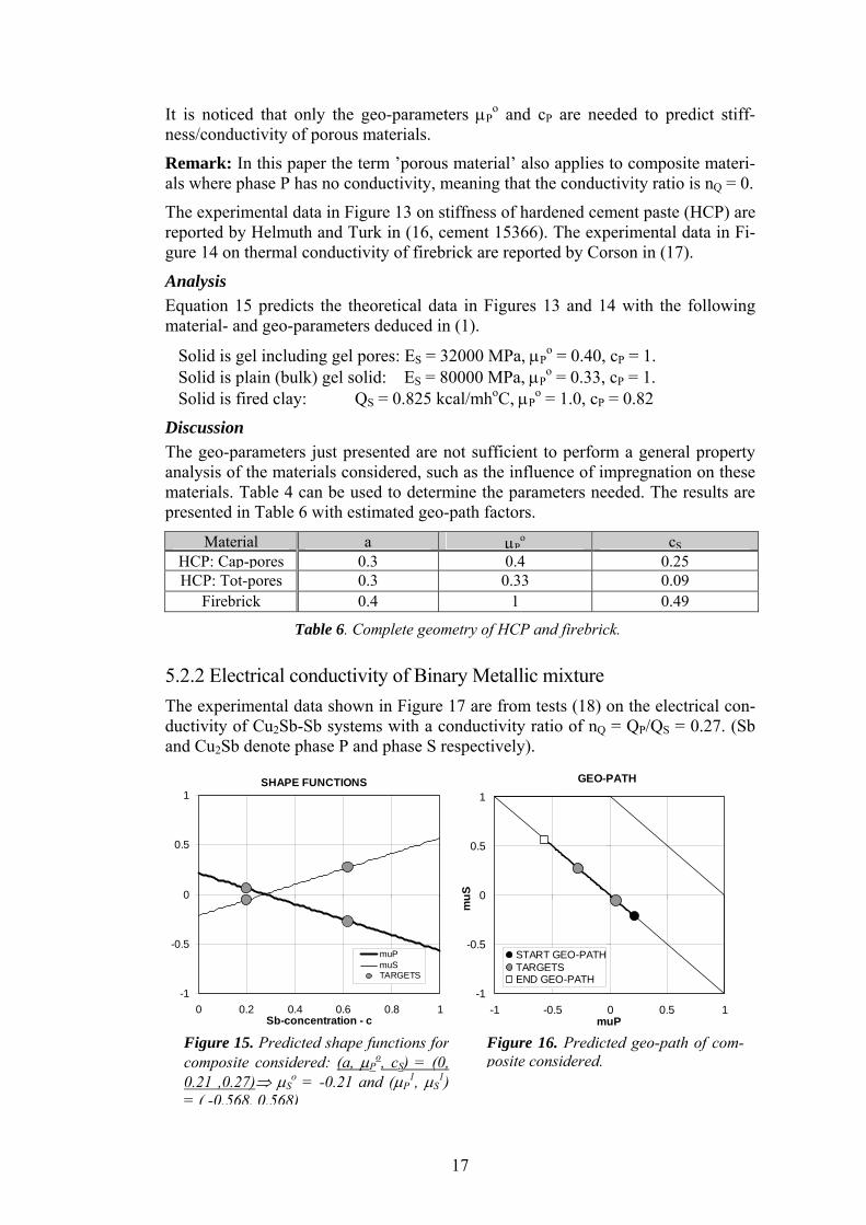
5.2.2 Electrical conductivity of Binary Metallic mixture The experimental data shown in Figure 17 are from tests (18) on the electrical con-ductivity of Cu2Sb-Sb systems with a conductivity ratio of nQ = QP/QS = 0.27. (Sb and Cu2Sb denote phase P and phase S respectively).

GEO-PATH

-1

-0.5

0

0.5

1

-1 -0.5 0 0.5 1muP

muS

START GEO-PATHTARGETSEND GEO-PATH

SHAPE FUNCTIONS

-1

-0.5

0

0.5

1

0 0.2 0.4 0.6 0.8 1Sb-concentration - c

muPmuSTARGETS

Figure 15. Predicted shape functions forcomposite considered: (a, µP

o, cS) = (0,0.21 ,0.27)⇒ µS

o = -0.21 and (µP1, µS

1)= ( -0.568, 0,568)

Figure 16. Predicted geo-path of com-posite considered.

17

Analysis Prescribed data sets are chosen to be (Q1,/Q2)/QS = (0.797,0.468) at (c1,c2) = (0.20, 0.62). Associated composite geometrical characteristics predicted are presented in Figures 15 and 16. For this geometry the solid line in Figure 17 presents the con-ductivities theoretically predicted for any Sb-concentration.

Discussion – processing model An excellent agreement is observed between experimental and predicted data. From comparing Figure 16 with Figure 5 can be estimated that the composite considered is a DC-CD composite with the following processing model: Sb-elements of disk shapes, A ≈ 0.08, are mixed with Cu2Sb-elements of disk shapes A ≈ 0.25.

EL-CONDUCTIVITY OF Cu2Sb-Sb

0

0.2

0.4

0.6

0.8

1

0 0.2 0.4 0.6 0.8 1Sb vol-concentration - c

q =

Q/Q

S

DESIGNHSEXP-STEPH

Figure 17. Electrical conductivity of bina-ry metallic mixture (Cu2Sb-Sb).

5.2.3 Stiffness of empty and impregnated HCP The experimental data shown in Figures 20 and 21 are from tests reported in (19,20) on the stiffness of hardened cement paste – before (empty HCP) and after impregnati-on with Sulphur respectively.

SHAPE FUNCTIONS GEO-PATH

0.5

1

0.5

1

18

Figure 19. Predicted geo-path for theHCP considered.

Figure 18. Predicted shape factors for theHCP considered: (a, µP

o, cS) = (0.4, 0.431, 0.082) ⇒ µS

o = -0.031 and (µP1, µS

1) = (0.053, 0.347)

-1

-0.5

0

-1 -0.5 0 0.5 1muP

muS

START GEO-PATHTARGETSEND GEO-PATH

-1

-0.5

0

0 0.2 0.4 0.6 0.8 1Capillary porosity - c

muPmuStargets

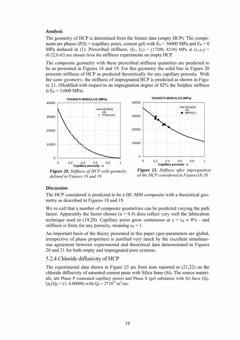
Analysis The geometry of HCP is determined from the former data (empty HCP): The compo-nents are phases (P,S) = (capillary pores, cement gel) with ES = 36000 MPa and EP = 0 MPa deduced in (1). Prescribed stiffness, (E1, E2) = (17200, 8210) MPa at (c1,c2) = (0.22,0.42) are chosen from the stiffness experiments on empty HCP.

The composite geometry with these prescribed stiffness quantities are predicted to be as presented in Figures 18 and 19. For this geometry the solid line in Figure 20 presents stiffness of HCP as predicted theoretically for any capillary porosity. With the same geometry, the stiffness of impregnated HCP is predicted as shown in Figu-re 21. (Modified with respect to an impregnation degree of 82% the Sulphur stiffness is EP = 11000 MPa).

Figure 21. Stiffness after impregnationof the HCP considered in Figures18-20.

YOUNG'S MODULUS (MPa)

0

10000

20000

30000

40000

0 0.2 0.4 0.6 0.8 1Capillary porosity - c

DESIGNHSPOROUS

YOUNG'S MODULUS (MPa)

0

10000

20000

30000

40000

0 0.2 0.4 0.6 0.8 1Capillary porosity - c

DESIGNHSIMPREG

Figure 20. Stiffness of HCP with geometry defined in Figures 18 and 19.

Discussion The HCP considered is predicted to be a DC-MM composite with a theoretical geo-metry as described in Figures 18 and 19.

We re-call that a number of composite geometries can be predicted varying the path factor. Apparently the factor chosen (a = 0.4) does reflect very well the fabrication technique used in (19,20). Capillary pores grow continuous at c = cS ≈ 8% - and stiffness is finite for any porosity, meaning cP > 1.

An important basis of the theory presented in this paper (geo-parameters are global, irrespective of phase properties) is justified very much by the excellent simultane-ous agreement between experimental and theoretical data demonstrated in Figures 20 and 21 for both empty and impregnated pore systems.

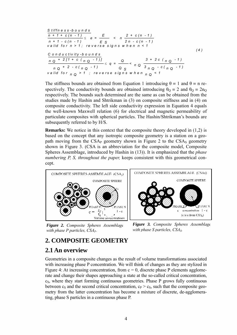
5.2.4 Chloride diffusivity of HCP The experimental data shown in Figure 23 are from tests reported in (21,22) on the chloride diffusivity of saturated cement paste with Silica fume (Si). The source materi-als, are Phase P (saturated capillary pores) and Phase S (gel substance with Si) have (QP, QS)/QP = (1, 0.00008) with QP = 2*10-9 m2/sec.

19

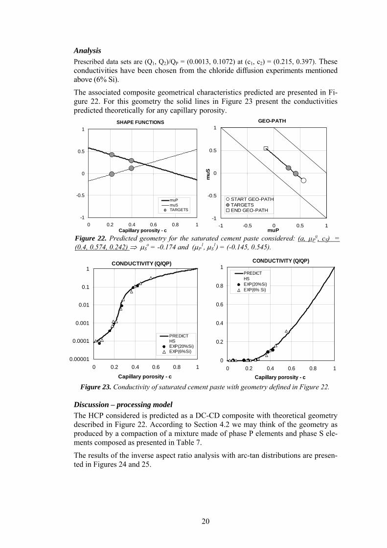
Analysis Prescribed data sets are (Q1, Q2)/QP = (0.0013, 0.1072) at (c1, c2) = (0.215, 0.397). These conductivities have been chosen from the chloride diffusion experiments mentioned above (6% Si).

The associated composite geometrical characteristics predicted are presented in Fi-gure 22. For this geometry the solid lines in Figure 23 present the conductivities predicted theoretically for any capillary porosity.

Figure 22. Predicted geometry for the saturated cement paste considered: (a, µPo, cS) =

(0.4, 0.574, 0.242) ⇒ µSo = -0.174 and (µP

1, µS1) = (-0.145, 0.545).

GEO-PATH

-1

-0.5

0

0.5

1

-1 -0.5 0 0.5 1muP

muS

START GEO-PATHTARGETSEND GEO-PATH

SHAPE FUNCTIONS

-1

-0.5

0

0.5

1

0 0.2 0.4 0.6 0.8 1Capillary porosity - c

muPmuSTARGETS

CONDUCTIVITY (Q/QP)

0.00001

0.0001

0.001

0.01

0.1

1

0 0.2 0.4 0.6 0.8 1

Capillary porosity - c

PREDICTHSEXP(20%Si)EXP(6%Si)

CONDUCTIVITY (Q/QP)

0

0.2

0.4

0.6

0.8

1

0 0.2 0.4 0.6 0.8 1Capillary porosity - c

PREDICTHSEXP(20%Si)EXP(6% Si)

Figure 23. Conductivity of saturated cement paste with geometry defined in Figure 22.

Discussion – processing model The HCP considered is predicted as a DC-CD composite with theoretical geometry described in Figure 22. According to Section 4.2 we may think of the geometry as produced by a compaction of a mixture made of phase P elements and phase S ele-ments composed as presented in Table 7.

The results of the inverse aspect ratio analysis with arc-tan distributions are presen-ted in Figures 24 and 25.

20

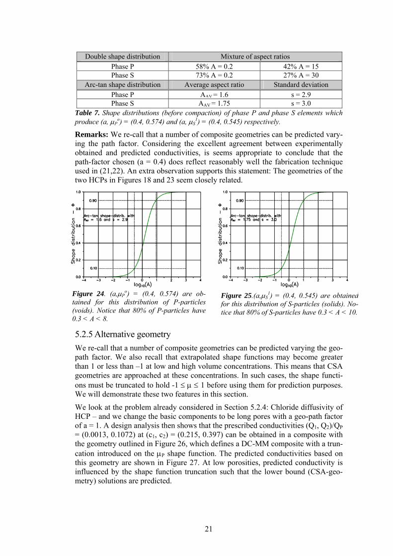
Table 7. Shape distributions (before compaction) of phase P and phase S elements which produce (a, µP

o) = (0.4, 0.574) and (a, µS1) = (0.4, 0.545) respectively.

Double shape distribution Mixture of aspect ratios Phase P 58% A = 0.2 42% A = 15 Phase S 73% A = 0.2 27% A = 30

Arc-tan shape distribution Average aspect ratio Standard deviation Phase P AAV = 1.6 s = 2.9 Phase S AAV = 1.75 s = 3.0

Remarks: We re-call that a number of composite geometries can be predicted vary-ing the path factor. Considering the excellent agreement between experimentally obtained and predicted conductivities, is seems appropriate to conclude that the path-factor chosen (a = 0.4) does reflect reasonably well the fabrication technique used in (21,22). An extra observation supports this statement: The geometries of the two HCPs in Figures 18 and 23 seem closely related.

Figure 24. (a,µPo) = (0.4, 0.574) are ob-

tained for this distribution of P-particles(voids). Notice that 80% of P-particles have0.3 < A < 8.

Figure 25.(a,µS1) = (0.4, 0.545) are obtained

for this distribution of S-particles (solids). No-tice that 80% of S-particles have 0.3 < A < 10.

5.2.5 Alternative geometry We re-call that a number of composite geometries can be predicted varying the geo-path factor. We also recall that extrapolated shape functions may become greater than 1 or less than –1 at low and high volume concentrations. This means that CSA geometries are approached at these concentrations. In such cases, the shape functi-ons must be truncated to hold -1 ≤ µ ≤ 1 before using them for prediction purposes. We will demonstrate these two features in this section.

We look at the problem already considered in Section 5.2.4: Chloride diffusivity of HCP – and we change the basic components to be long pores with a geo-path factor of a = 1. A design analysis then shows that the prescribed conductivities (Q1, Q2)/QP = (0.0013, 0.1072) at (c1, c2) = (0.215, 0.397) can be obtained in a composite with the geometry outlined in Figure 26, which defines a DC-MM composite with a trun-cation introduced on the µP shape function. The predicted conductivities based on this geometry are shown in Figure 27. At low porosities, predicted conductivity is influenced by the shape function truncation such that the lower bound (CSA-geo-metry) solutions are predicted.

21

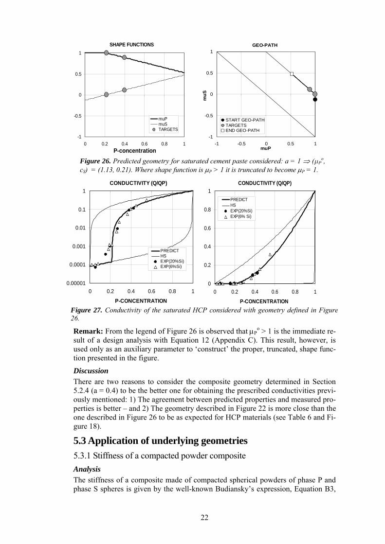
Figure 26. Predicted geometry for saturated cement paste considered: a = 1 ⇒ (µPo,

cS) = (1.13, 0.21). Where shape function is µP > 1 it is truncated to become µP = 1.

SHAPE FUNCTIONS

-1

-0.5

0

0.5

1

0 0.2 0.4 0.6 0.8 1P-concentration

muPmuSTARGETS

GEO-PATH

-1

-0.5

0

0.5

1

-1 -0.5 0 0.5 1muP

muS

START GEO-PATHTARGETSEND GEO-PATH

Figure 27. Conductivity of the saturated HCP considered with geometry defined in Figure26.

CONDUCTIVITY (Q/QP)

0

0.2

0.4

0.6

0.8

1

0 0.2 0.4 0.6 0.8 1

P-CONCENTRATION

PREDICTHSEXP(20%Si)EXP(6% Si)

CONDUCTIVITY (Q/QP)

0.00001

0.0001

0.001

0.01

0.1

1

0 0.2 0.4 0.6 0.8 1

P-CONCENTRATION

PREDICTHSEXP(20%Si)EXP(6%Si)

Remark: From the legend of Figure 26 is observed that µPo > 1 is the immediate re-

sult of a design analysis with Equation 12 (Appendix C). This result, however, is used only as an auxiliary parameter to ‘construct’ the proper, truncated, shape func-tion presented in the figure.

Discussion There are two reasons to consider the composite geometry determined in Section 5.2.4 (a = 0.4) to be the better one for obtaining the prescribed conductivities previ-ously mentioned: 1) The agreement between predicted properties and measured pro-perties is better – and 2) The geometry described in Figure 22 is more close than the one described in Figure 26 to be as expected for HCP materials (see Table 6 and Fi-gure 18).

5.3 Application of underlying geometries 5.3.1 Stiffness of a compacted powder composite Analysis The stiffness of a composite made of compacted spherical powders of phase P and phase S spheres is given by the well-known Budiansky’s expression, Equation B3,

22

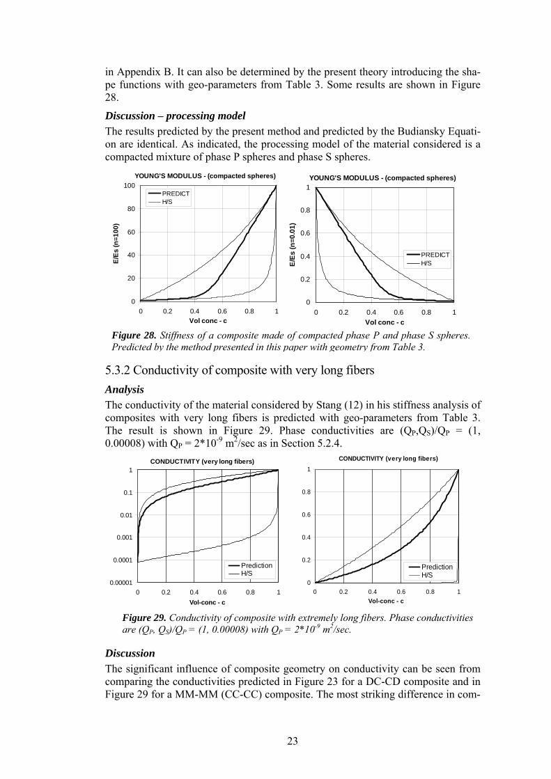
in Appendix B. It can also be determined by the present theory introducing the sha-pe functions with geo-parameters from Table 3. Some results are shown in Figure 28.

Discussion – processing model The results predicted by the present method and predicted by the Budiansky Equati-on are identical. As indicated, the processing model of the material considered is a compacted mixture of phase P spheres and phase S spheres.

YOUNG'S MODULUS - (compacted spheres)

0

20

40

60

80

100

0 0.2 0.4 0.6 0.8 1Vol conc - c

E/Es

(n=1

00)

PREDICTH/S

YOUNG'S MODULUS - (compacted spheres)

0

0.2

0.4

0.6

0.8

1

0 0.2 0.4 0.6 0.8 1Vol conc - c

E/E

s (n

=0.0

1)

PREDICTH/S

Figure 28. Stiffness of a composite made of compacted phase P and phase S spheres.Predicted by the method presented in this paper with geometry from Table 3.

5.3.2 Conductivity of composite with very long fibers Analysis The conductivity of the material considered by Stang (12) in his stiffness analysis of composites with very long fibers is predicted with geo-parameters from Table 3. The result is shown in Figure 29. Phase conductivities are (QP,QS)/QP = (1, 0.00008) with QP = 2*10-9 m2/sec as in Section 5.2.4.

CONDUCTIVITY (very long fibers)

0.00001

0.0001

0.001

0.01

0.1

1

0 0.2 0.4 0.6 0.8 1Vol-conc - c

PredictionH/S

CONDUCTIVITY (very long fibers)

0

0.2

0.4

0.6

0.8

1

0 0.2 0.4 0.6 0.8 1Vol-conc - c

PredictionH/S

Figure 29. Conductivity of composite with extremely long fibers. Phase conductivitiesare (QP, QS)/QP = (1, 0.00008) with QP = 2*10-9 m2/sec.

Discussion The significant influence of composite geometry on conductivity can be seen from comparing the conductivities predicted in Figure 23 for a DC-CD composite and in Figure 29 for a MM-MM (CC-CC) composite. The most striking difference in com-

23

posite geometries between these two composites is the absence of interaction be-tween fibers in the latter composite; see Section 2.3.4 and Appendix B.

6. CONCLUSION AND FINAL REMARKS A theory has been presented in this paper, by which properties can be predicted for composites with arbitrary phase geometries.

The theory is inversed to predict which type of phase geometries will create prescri-bed material properties.

Both versions of the theory are applied successfully on examples of practical rele-vance, such as: Electrical conductivity of binary metallic mixture, Stiffness of emp-ty and impregnated HCP (hardened cement paste), and Chloride diffusivity of HCP.

Future research: Much research has still to be made in the area of composite geo-metry. Especially, in the field of ‘translating’ theoretical geo-descriptions to de-scriptions which can be realized in practice. Some suggestions, which still have to be further justified, are made in Section 4.2 and exemplified in Sections 5.2.2, 5.3.1, and 5.2.4.

In order to improve/modify the methods presented in this paper, a combined re-search effort must be made involving both theoretical, including FEM, and techno-logical/experimental means. Research is also needed with respect to shape distribu-tions versus size distributions of phase elements.

7. NOTATIONS We notice that the notation used in this paper is similar to the one used in (1). The list does not consider less general symbols, which are explained locally. Notations used by

the author prior to his work in (1) are somewhat different. Abbreviations and subscripts V Volume P Phase P S Phase S No subscript Composite materials H/S Hashin/Shtrikman's property bounds EST Estimate Geo-parameters c = VP/(VP+VS) Volume concentration of phase P µo,µ1 Shape factors µP,µS Shape functions a Geo-path factor cP,cS Critical concentrations θ Geo-function for stiffness θQ Geo-function for conductivity Stiffness and other properties E Stiffness (Young's modulus) e = E/ES Relative stiffness of composite n = EP/ES Stiffness ratio

24

Q Conductivity (e.g. thermal, electrical, diffusivity) q = Q/QS Relative conductivity of composite nQ = QP/QS Conductivity ratio Stress and strain σ External mechanical stress σP Phase P stress caused by external mechanical stress σS Phase S stress caused by external mechanical stress λ Linear eigenstrain (e.g. shrinkage, thermal expansion) ∆λ = λP-λS Linear differential eigenstrain ρ Hydrostatic stress caused by eigenstrain

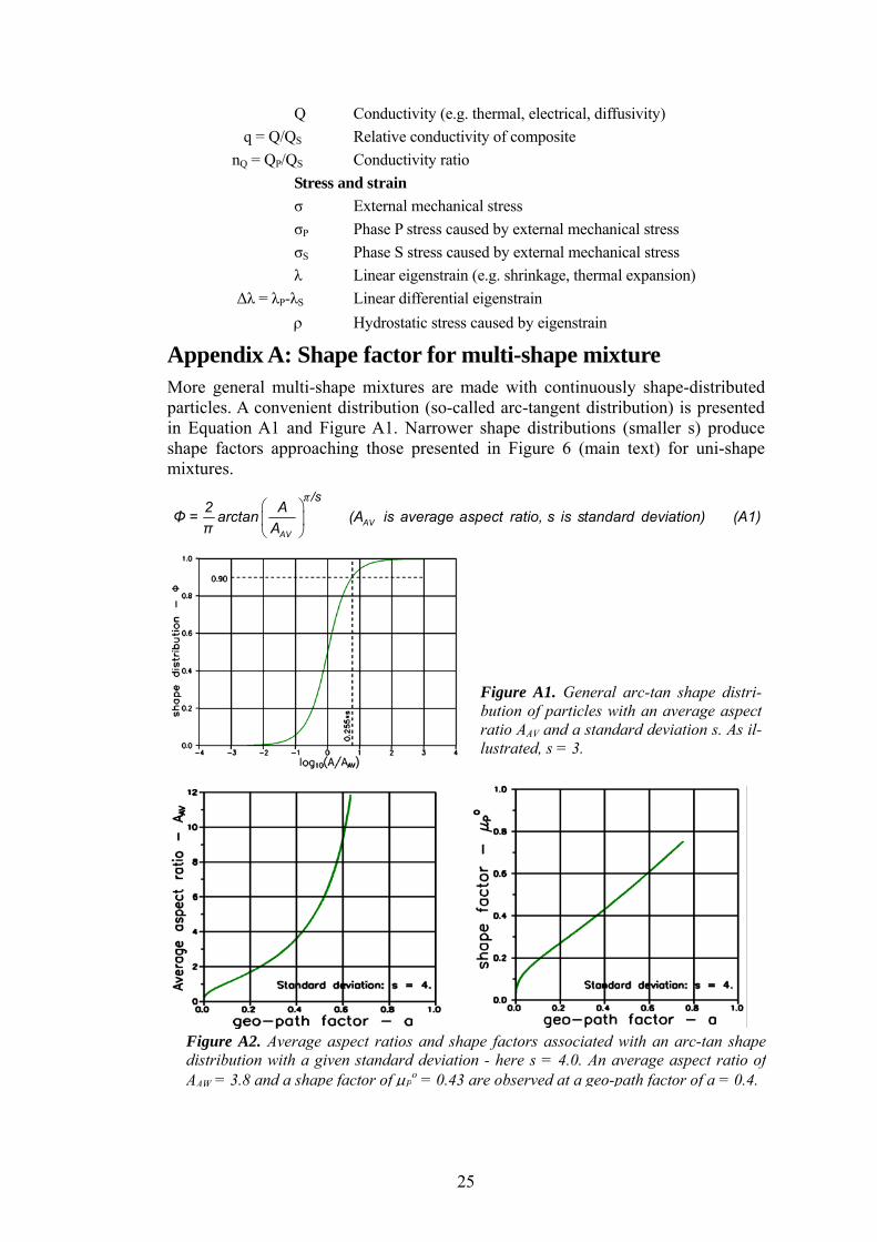
Appendix A: Shape factor for multi-shape mixture More general multi-shape mixtures are made with continuously shape-distributed particles. A convenient distribution (so-called arc-tangent distribution) is presented in Equation A1 and Figure A1. Narrower shape distributions (smaller s) produce shape factors approaching those presented in Figure 6 (main text) for uni-shape

⎛ ⎞⎜ ⎟⎝ ⎠

AVAV

/s2 AΦ = arctan (A is average aspect ratio, s is standard deviation) (A1)π A

π

mixtures.

Figure A1. General arc-tan shape distri-bution of particles with an average aspectratio AAV and a standard deviation s. As il-lustrated, s = 3.

Figure A2. Average aspect ratios and shape factors associated with an arc-tan shape distribution with a given standard deviation - here s = 4.0. An average aspect ratio of AAW = 3.8 and a shape factor of µP

o = 0.43 are observed at a geo-path factor of a = 0.4.

25

For a given standard distribution, s, the results of a multi-shape analysis can be or-ganized as demonstrated in Figure A2 from which the shape factor, µP

o, and the fi-nal shape distribution with average aspect ratio, Aon of the geo-path factor, a.

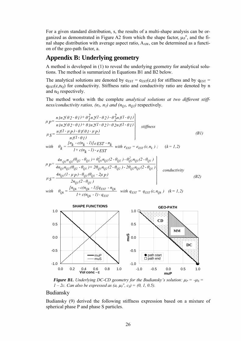
2 2( - ) + (1 - ) - (1 - )n n θ θ θ n θ θ n θ1 2 2 1 2 2 1 1 ⎫⎪⎪1 2 = µ P ( - ) + (1 - ) - (1 - )n n θ θ θ n θ θ n θ1 2 2 1 1 2 2 2 1 1 stiffness(1 - ) - ( - )µ µn θ θ1 1 1P P = µ S (1 - )n θ1 1

[n - c(n - 1)] - neESTk k kwith θ = k 1 + c(n - k

⎪⎪⎪⎪⎬⎪⎪⎪⎪⎪⎪⎭

(EST EST k

(B1)

with e = e (c,n ) ; k = 1,2)1) - e EST

2 2Q2 Q1 Q1 Q2 Q2 Q2 Q1 Q1Q1 Q2

Q1 Q2 Q2 Q1 Q1 Q2 Q2 Q2 Q1 Q1

Q1 Q1 Q1

Q1 Q1

Qk

(θ - θ ) + θ n (2 - θ ) - θ n (2 - θ )4n n = µ P 4n n (θ - θ ) + 2θ n (2 - θ ) - 2θ n (2 - θ )

conductivity4n (1 - ) - θ (θ - )µ 2µP P = µ S 2n (2 - θ )

with θ

⎫⎪⎪⎪⎪⎪⎪⎪⎬⎪⎪⎪⎪⎪⎪⎪⎭Qk Qk EST Qk

EST EST QkQk EST

(B2)

[n - c(n - 1)]q - n = with q = q (c,n ) (k = 1,2)

1 + c(n - 1) - q

AW, can be determined as a functi-

u lyi

ns are denoted by eEST = eEST(c,n) for stiffness and by qEST =

The method works with the complete analytical solutions at two different stiff-ness/conductivity ratios, (n1, n2) and (nQ1, nQ2) respectively.

Budiansky (9) derived the following stiffness expression based on a mixture of spherical phase P and phase S particles.

Appendix B: Underlying geometry A method is developed in (1) to reveal the nder ng geometry for analytical solu-tions. The method is summarized in Equations B1 and B2 below.

The analytical solutioqEST(c,nQ) for conductivity. Stiffness ratio and conductivity ratio are denoted by n and nQ respectively.

SHAPE FUNCTIONS

-1.0

-0.5

0.0

0.5

1.0

Budiansky

0.0 0.2 0.4 0.6 0.8 1.0Vol conc - c

muPmuS

GEO-PATH

-1.0

-0.5

0.0

0.5

1.0

muP

muS

-1.0 -0.5 0.0 0.5 1.0

path startpath end

Figure B11 – 2c. Ca

. Underlying DC-CD geometry for the Budiansky’s solution: µP = -µS =n also be expressed as (a, µP

o, cS) = (0, 1, 0.5).

MM

DC

CD

26

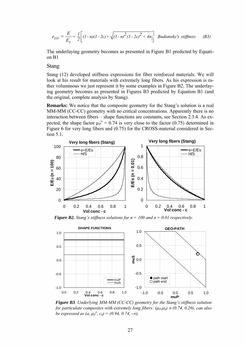
⎡ ⎤⎢ ⎥⎣ ⎦EST

S

1 2 2= (1 - n)(1 - 2c)+ (1 - n) (1 - 2c) + 4n Budiansky's stiffness (B3)2Ee =E

The underlaying geometry becomes as presented in Figure B1 predicted by Equati-on B1

Stang Stang (12) developed stiffness expressions for fiber reinforced materials. We will look at his result for materials with extremely long fibers. As his expression is ra-ther voluminous we just represent it by some examples in Figure B2. The underlay-ing geometry becomes as presented in Figures B3 predicted by Equation B1 (and the original, complete analysis by Stang).

Remarks: We notice that the composite geometry for the Stang’s solution is a real MM-MM (CC-CC) geometry with no critical concentrations. Apparently there is no interaction between fibers – shape functions are constants, see Section 2.3.4. As ex-pected, the shape factor µP

o = 0.74 is very close to the factor (0.75) determined in Figure 6 for very long fibers and (0.75) for the CROSS-material considered in Sec-tion 5.1.

Very long fibers (Stang)

0

0.2

0.4

0.6

0.8

1

0 0.2 0.4 0.6 0.8 1Vol conc - c

E/Es

(n =

0.0

1)

e=E/EsH/S

Very long fibers (Stang)

0

20

40

60

80

100

0 0.2 0.4 0.6 0.8 1Vol conc - c

E/E S

(n =

100

)

e=E/EsH/S

Figure B2. Stang’s stiffness solutions for n = 100 and n = 0.01 respectively.

SHAPE FUNCTIONS

-1.0

-0.5

0.0

0.5

1.0

0.0 0.2 0.4 0.6 0.8 1.0Vol conc - c

muPmuS

GEO-PATH

-1.0

-0.5

0.0

0.5

1.0

-1.0 -0.5 0.0 0.5 1.0muP

muS

path startpath end

Figure B3. Underlying MM-MM (CC-CC) geometry for the Stang’s stiffness solutionfor particulate composites with extremely long fibers: (µP,µS) ≡ (0.74, 0.20), can alsobe expressed as (a, µP

o, cS) = (0.94, 0.74, -∞).

27

Appendix C: Numerical determination of shape functions The general expressions for deducing composite geometries from prescribed com-posite properties, stiffness and conductivity, is presented in Equation 12, Section 4.1. The following expressions reveal geometry from two data sets, (c1, e1), (c2, e2), for stiffness and two data sets, (c1, q1), (c2, q2), for conductivity respectively.

;

[n - c (n - 1)]e - nk kθ = (k = 1,2)k 1+ c (n - 1) - ek kn(1 - a)+ θ (a - θ )k kµ = ; µ = a - µ (k = 1,2) (C1)Sk Pk Skθ (1 - n)k

c µ - c µc µ - c µ c µ - c µ2 S1 1 S2o o o2 P1 1 P2 2 P1 1 P2µ = ; µ = a - µ c = ; c =P P PS Sc - c µ - µ µ - µ2 1 S1 S2 P1 P2

;

[n - c (n - 1)]q - nQ Q Qk kθ = (k = 1,2)Qk 1+ c (n - 1) - qQk k4n (1 - a)+ θ (2a - θ )Q Qk Qk

µ = ; µ = a - µ (k = 1,2) (C2)Sk Pk Sk2θ (1 - n )QQkc µ - c µc µ - c µ c µ - c µ2 S1 1 S2o o o2 P1 1 P2 2 P1 1 P2µ = ; µ = a - µ c = ; c =P P PS Sc - c µ - µ µ - µ2 1 S1 S2 P1 P2

8. LITERATURE

1. Nielsen, L. Fuglsang: "Composite Materials – Properties as influenced by phase geometry", Springer Verlag, Berlin, Heidelberg 2005. 2. Idem: "Elastic Properties of Two-Phase Materials", Materials Science and Enginee-ring, 52(1982), 39-62. 3. Hashin, Z. and Shtrikman, S.: "Variational approach to the theory of elastic behavior of multi-phase materials". J. Mech. Solids, 11(1963), 127 - 140. 4. Idem: "A variational approach to the theory of the effective magnetic permeability of multi-phase materials", J. Appl. Phys. 33(1962), 3125. 5. Hill, R.: "Elastic properties of reinforced solids: Some theoretical principles". J. Mech. Phys. Solids, 11(1963), 357 - 372. 6. Maxwell, J.C.: Treatise on electricity and magnetism, 1(1873), 365. 7. Böttcher, C.J.F.: "The dielectric constant of crystalline powders", Rec. Trav. Pays-Bas, 64(1945), 47. 8. Landauer, R.: ”The electric resistance of binary metallic mixtures”, J. Appl. Phys, 23(1952), 779. 9. Budiansky, B.: On the elastic moduli of some heterogeneous materials". J. Mech. Phys. Solids, 13(1965), 223 - 227. 10. Christoffersen, J.: ”Elastic and elastic-plastic composites – a new approach”, DCAMM, Rep. 61(1973), (Danish Centre for Applied Mathematics and Mechanics, Tech. Univ. Denmark). 11. Levin, V.M.: ”Determination of effective elastic moduli of composite materials”, Sov. Phys. – Dokl., 20(1975), 147.

28

12. Stang, Henrik: "En kompositmaterialeteori og dens anvendelse til beskrivelse af trækpåvirkede cementkompositter" (in Danish, "A composite theory and its application to cement based composites subjected to tension"), Thesis, Institute of Structural Mechanics, Tech. Univ. Denmark, 1984. 13. Hashin, Z.: "Elastic moduli of heterogeneous materials". J. Appl. Mech., 29 (1962), 143 - 150. 14. Idem: "Assessment of Self Consistent Scheme approximation: Conductivity of parti-culate composites", J. Compos. Mater. Vol 2(1968), 284. 15. Nielsen, L. Fuglsang: “Finite Element Analysis of two basic Composites”, Docu-mentation report R-089(2004), Dept. of Civ. Eng., Technical University of Denmark. 16. Helmuth, R.A. and D.H. Turk: "Elastic moduli of hardened Portland cement and Tricalcium silicate pastes: Effects of porosity", pp. 135-144 in Symposium on structure of Portland cement and concrete. Highw. Res. Bd., Spec. Rept., No. 90, 1966. 17. Corson, P. B.: "Correlation functions for predicting properties of heterogeneous materials, IV: Effective thermal conductivity of two-phase solids", J. Appl. Phys. (USA) 45 (1974), 3180. 18. Stephens, E. and Evans, E.J.: 'The Hall effect and other properties of copper-anti-mony series of alloys', Phil. Mag. 7(1929), 161. 19. Beaudoin, J.J. and R.F. Feldman: "A study of mechanical properties of autoclaved Calcium silicate systems", Cem. Concr. Res., 5(1975), 103-118. 20. Feldman, R.F. and J.J. Beaudoin: “Studies of composites made by impregnation of porous bodies. I: Sulphur impregnant in Portland cement systems", Cem. Concr. Res., 7(1977), 19-30. 21. Bentz, D.P., O.M. Jensen, A.M. Coats, and F.P. Glasser: "Influence of silica fume on diffusivity in cement-based materials. Part I: Experimental and computer modeling stu-dies on cement pastes", Cement and Concrete Research, 30(2000), 953-962. 22. Jensen, O.M.: "Chloride ingress in cement paste and mortar measured by Electron Probe Micro Analysis", Report R51(1998), Department of Structural Engineering and Ma-terials, Technical University of Denmark

29