Download pdf - ANALOG VLSI SYSTEM FOR ACTIVE DRAG REDUCTIONid3490.securedata.net/rod/pdf/RG.Paper.BC13.pdf4 ANALOG VLSI SYSTEM FOR ACTIVE DRAG REDUCTION Vincent Koosh, Bhusan Gupta, Dave Babcock,

4 ANALOG VLSI SYSTEM FORACTIVE DRAG REDUCTION

Vincent Koosh, Bhusan Gupta, Dave Babcock,

Rodney Goodman, Fukang Jiang, Yu-Chong Tai,

Steve Tungy and Chih-Ming Hoy

Dept. of Electrical EngineeringCalifornia Institute of Technology, Pasadena, CA 91125

fdarkd,bgupta,babcock,[email protected]

yDepartment of Mechanical and Aerospace EngineeringUniversity of California, Los Angeles CA 90024

We describe an analog CMOS VLSI system that can process real-time signals fromshear stress sensors to detect regions of high shear stress along a surface in an airflow.The outputs of the CMOS circuit control the actuation of micromachined flaps with thegoal of reducing this high shear stress on the surface and thereby lowering the totaldrag. We have designed, fabricated, and tested parts of this system in a wind tunnel inboth laminar and turbulent flow regimes. The implemented system includes adaptivecircuits for temperature stabilization in the shear stress microsensors and global gaincontrol in the microactuators.

4.1 INTRODUCTION

In today’s cost-conscious air transportation industry, fuel costs are a substantial eco-nomic concern. Drag reduction is an important way to increase fuel efficiency whichreduces these costs. Even a 5% reduction in drag can translate into estimated savingsof millions of dollars in annual fuel costs.

Organized structures which play an important role in turbulence transport maycause large skin friction drag. Commonly observed near-wall streamwise vorticescause high drag in turbulent flows (Figure 4.1). The interaction of these vortices,

81

82 LEARNING ON SILICON

Flow into pageCounter-rotating vortices

Region of high shear stress

Spanwise Direction

Figure 4.1 Diagram of the interaction between a vortex pair and the wall showing thehigh shear stress (hence drag) region created by the pair of counter- rotating streamwisevortices.

which appear randomly in both space and time, with the viscous layer near a surfacecreates regions of high surface shear stress. This shear stress, when integrated over asurface, contributes to the total drag. Attempts to reduce drag by controlling turbulentflows have focused on methods of either preventing the formation or mitigating thestrength of these vortices. The microscopic size of these vortices, which decreases asthe Reynolds number of the flow increases, has limited physical experimentation, andthe inherent complexity of the non-linear Navier-Stokes equations has likewise limitedthe analytical approaches.

4.2 CAN BIOLOGY TELL US SOMETHING?

Figure 4.2 Examples of shark scales (white bar = 25�m).

In many complex problems, one can often find inspiration by observing how naturehas evolved biological systems to address the problem. For drag reduction, deep sea

ACTIVE DRAG REDUCTION 83

sharks serve as a potential biological model because they are a highly evolved predatorwith a 350 million year old lineage. Deep-sea sharks (for example, hammerheadsharks) can swim up to 20 meters per second (72 km per hr) in deep water. The exactphysiology of these species remains a mystery because they are difficult to study as thedeep sea setting is hard to replicate in a controlled environment. Biologists do know,however, something about the scales (dermal denticles) that cover the shark’s skin.Only recently researchers [1] found that the denticles have microscopic structure tothem (Figure 4.2). The natural argument about evolution would lead one to concludethat the structure of these scales assists the sharks’ movement, perhaps indicating somemethod of drag reduction.

4.2.1 Active Control

The entire question of active control of shark skin is very much a speculative one.Biologists hypothesize [2] that sharks can actively move their denticles. The indirectevidence of this is twofold. One, the denticles connect to muscles underneath theshark’s skin. Two, the total number of mechano-receptive pressure sensors (pit organs)and their placement on a shark’s body positively correlates with the speed of the species.For good active control the shark may need many sensors to relay the current conditionover its body. However, questions remain about sharks utilizing active control. Theconclusion that one can draw from this example of biology is that it may be beneficialto employ controlled microscopic structures to reduce the drag.

4.3 HOW SMALL IS SMALL?

By examining drag patterns in our wind tunnel at velocities between 10 and 20 m/s(36 and 72 km/hr), one can narrow the scope of the problem in order to extract useablestatistics. The drag-inducing vortex pair streaks vary as the Reynolds number of theflow changes. For a typical airflow of 15 meters per second (54 km/hr) in the windtunnel, the Reynolds number is about 104. This, in turn, gives the vortex streaks astatistical mean width of about 1 millimeter. The length of a typical vortex streak canbe about 2 centimeters giving the streaks a twenty to one aspect ratio. The averagespacing between streaks is about 2.5 millimeters. The mean rate of appearance of thestreaks is approximately 100 Hz. The appearance and disappearance of these vortexpairs can best be described by a chaotic process.

4.4 NEURAL NETWORK BASED CONTROL

Previous numerical simulations [3] demonstrated that suppressing the interaction be-tween streamwise vortices and the wall achieves significant drag reduction (on theorder of about 25%). These computational fluid dynamics’ experiments incorporate


y+=10

Flow into pageCount er- rot at ing vort ices

Surface

Actuat ion = -v(y+=10)

Figure 4.3 Simple control law which demonstrates the required actuation at the wallboundary to achieve a significant drag reduction.

active feedback control to achieve this goal. The control scheme used in the experi-ments involved blowing and suction at the wall according to the normal component ofthe velocity field. This normal component (�v(y+ = 10)) is sensed in the near-wallregion away from the surface (see Figure 4.3). The problem with these techniques isthat it requires information about the velocity away from the wall. This information isvery difficult to obtain in a real system.

(dw/dy)

Inputlayer

(vwall )

Surface ShearStress

Hiddenlayer

Outputlayer

Actuation

Figure 4.4 Neural Network Architecture.

Thus, an adaptive controller based on a neural network [10] that does not requirevelocity information away from the wall was implemented. A two layer shared weightneural network consisting of hyperbolic tangent non-linear hidden units and linearoutput units to predict similar actuation using only surface measurable quantities, i.e.surface shear stresses, was developed (Figure 4.4). Training off-line with data from thenear-wall controlled experiments, the neural network extracted a pattern that predictsthe local actuation to be proportional to the spanwise derivative of the spanwise shearstress in the surrounding region (Figure 4.6). The same network was then appliedat each grid point in the input (surface spanwise shear stress) array to generate thecorresponding output (actuation) array.


Plant

Σ

NNInverse

Plant Model

NNControllerdesired

(dw/dy)

modelerror

Weight Copy

dw/dyv(y+=0) predictedv(y+=0)

+

-

∂∂ η

∂∂

η

w

y

w

yt t

=

< <+1

0 1

Figure 4.5 Adaptive Inverse Model Scheme for Neural Controller

Figure 4.6 Learned Weight Pattern. Wj = A 1�cos�jj

This neural controller was applied in an on-line adaptive inverse model scheme(Figure 4.5) We observed that the relative magnitudes of the weights did not change(indicating the approximate derivative pattern is preserved) but that the absolute mag-nitudes fluctuated during the course of the simulation. Therefore the input weightswere fixed to compute an approximation to the derivative leaving only a gain and biasfor each layer to adapt as the simulation progresses.

Applying this control network and employing blowing and suction at the wall basedonly on the wall shear stresses in the spanwise direction, was shown to reduce theskin friction by as much as 20% in direct numerical simulations of a low-Reynoldsnumber turbulent channel flow (Figure 4.7). Also, since a stable pattern was observedin the distribution of weights associated with the neural network, it was possible toderive a simple control scheme that produced the same amount of drag reduction. This


Figure 4.7 Numerical experiment of skin friction reduction

simple control scheme generates optimum wall blowing and suction proportional toa local sum of the wall shear stress in the spanwise direction. The distribution ofcorresponding weights is simple and localized, thus making real implementation morestraightforward.

Although this work is a significant improvementover earlier approaches that requirevelocity information within the flow, there are still a number of technical issues beforesuch a control scheme can be implemented in real practice. Among other things,precise control of blowing and suction distributed over a surface in a laboratory test isstill too difficult to implement.

However, it appears that a simple control law that pushes the areas of high shearstress away from the wall is beneficial to minimizing the overall drag. This observationforms the basis for the system that we wish to build.

4.5 SYSTEM DETAILS

We want to combine the technologies of silicon micromachining and analog VLSI tobuild an integrated system which actively strives to reduce the drag along its surface.


Fluid Flow

ActuatorsProcessing

Sensors

analog VLSI control system

surface

Figure 4.8 Schematic diagram of our proposed system.

Micromachining technology allows construction of fluid sensors and actuators on thesame scale as the vortex pairs. Analog VLSI affords us the ability to build densecircuits which do the real-time processing necessary for an integrated system.

The goal is to design a system (Figure 4.8) that incorporates VLSI control circuitryalong with microscopic sensors and actuators and control circuitry that can activelydeform its surface to reduce drag.

Sensors Actuators

Control Circuitry

Airflow

Figure 4.9 Simplified diagram of the hardware system.

Figure 4.9 shows the desired physical layout of our system — both sensors andactuators cover the surface controlled by circuitry underneath.

Circuits process the signals from the sensors to find regions of high shear stress. Thisdetection process uses information about the spatial and temporal nature of the streaks.First, the long and narrow aspect ratio leads to building "column"-oriented templates forstreak detection. We organize the sensor outputs into thin feature detectors orientedin the direction of the airflow. When several sensors in a column register either alarger or smaller output than their neighbors in a spanwise direction, this differenceaccumulates. If this accumulated difference exceeds a threshold, a vortex pair streakmay be present in that column. The appropriate control action raises the associatedactuator.


4.6 MICROMACHINED COMPONENTS

The microsensors and microactuators [4,5,6,11] employ silicon micromachining tech-nology.

4.6.1 Shear Stress Sensor

Figure 4.10 Shear stress sensor showing polysilicon wire over diaphragm.

The microsensor (Figure 4.10) allows measurement of the heat transfer between aheated wire and the air. Heat transfers by convection from the electrically heated wireto the fluid flow causing a power change in the polysilicon wire. The polysilicon wiresits on a 200�m square, 1.2�m thick silicon nitride diaphragm over a vacuum cavity.The 2.0�m deep vacuum cavity serves to minimize thermal losses to the substrate.The sensitivity of the sensor with a cavity underneath is on the order of 10’s of mV/Pa.This is approximately an order of magnitude larger than what is attainable without thecavity.

A discrete constant temperature (CT) circuit (Figure 4.11) controls the shear stresssensor. The circuit maintains a constant temperature on the heated wire by means ofbalancing a bridge. The amplified voltage feedback signal is the output. The overallgain of the CT circuit is about 20.

We build the sensors as one row of 25 sensors (Figure 4.12). This allows monitoringof a spanwise section of the wind tunnel. Five sensor outputs (in the middle) provideinputs to the detection/control chip. Because we have many fewer actuators thansensors, it is unnecessary to use more sensors in the detection experiments.


OUT

+V

-V

Shear StressSensor

+V

-V

Figure 4.11 Constant Temperature Circuit for the Shear Stress Sensor

Figure 4.12 Array of shear stress sensors.

Figure 4.13 Photograph of a microactuator and an array of microactuators.

4.6.2 Microactuator

The microactuator (Figure 4.13) [7] is a thin plate raised via magnetic actuation.Current through a coil of metal in the external magnetic field is enough to causemillimeters of deflection.


Figure 4.14 Variation of the shear stress coefficient, CDN , with actuator frequency,!, and maximum actuator tip height, d. The solid O markers correspond to an !d of80 and the solid square markers correspond to an !d of 100.

How the motion of the streamwise vortices is affected by the actuator and even-tually achieves skin-friction reduction is a key issue for interactive wall flow control.Experiments have been carried out to investigate the interaction between a single highshear-stress streak and a micromachined actuator(Figure 4.14). Experiments are per-formed for different combinations of actuator frequency (!) and maximum tip height(d). As expected, the non-linear interaction between a moving surface and a vortex iscomplex. On the other hand, skin-friction reduction can be achieved if the actuationis properly applied. The reduction is a function of the product of! andd. Since theproduct of! andd is a measurement of the transverse velocity of the actuator flap,this result indicates that the amount of shear stress reduction is directly related to thetransport of high-speed fluid away from the surface by the vertical motion actuator.

4.7 EDGE DETECTION/CONTROL CIRCUITS

The first control circuits that were developed were only loosely based on what waslearned from the neural network simulation. Their main goal was to detect a largeenough edge in the shear stress profile which would then activate the actuators. Fig-ure 4.15 shows a diagram of how the information flows in the edge detection/controlchip. A non-linear filtering network connects together the amplified outputs of theshear stress sensors. The filtering preserves large differences between adjacent sensorswhile smoothing away small differences. The comparison and aggregation operations


Compare&

Aggregate

Actuator

CTSensor& Amp

Summed ColumnActivity

NonlinearFilter

Threshold Unit

CTSensor& Amp

CTSensor& Amp

Compare&

Aggregate

Figure 4.15 Block diagram of the complete edge detection/control chip.

correspond to different actuators by columns. Once the aggregated signal exceeds athreshold, the system drives the actuator.

Actuator

Anti-Bump

NonlinearFilter

Amplifier

Threshold Unit

ConstantTemperature

Sensor

Buffer

Anti-Bump

NonlinearFilter

Figure 4.16 Schematic of one column (channel) of the threshold detection/controlcircuitry


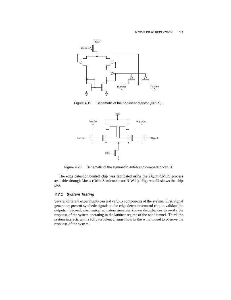
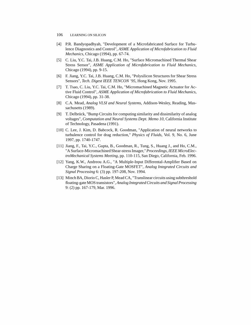
Figure 4.16 depicts a detailed schematic of a single column (or channel). TheCT output sensor signal feeds into a further stage of amplification (Figure 4.17). Abuffer (Figure 4.18) distributes the amplified signal to a non-linear resistive networkcomposed of the HRES circuits [8] (Figure 4.19). Sensor outputs in the same columnand sensor outputs in adjacent columns use different spatial filtering constants. Thedifferent constants serve to reinforce activity within a column and discourage activitybetween adjacent columns. The filtered signals feed to a symmetric anti-bump circuit[9] (Figure 4.20). The circuit’s operation mimics a soft comparator with an adjustabledead zone. The function of the circuit is to indicate when a particular column hasregistered a large shear stress value while the neighboring columns have not. Theoutput of the anti-bump circuit, a current, accumulates for a particular column andcompared to a threshold using the circuit in Figure 4.21. If the accumulated valueexceeds the threshold, the circuit triggers the actuator by turning on a pull-downtransistor.

RefBias

IN

OUTRef In

BIAS

Cin

VDD

Figure 4.17 Schematic of the first stage amplifier.

IN

OUT

BIAS

VDD

Figure 4.18 Schematic of a rail to rail buffer amplifier.


BIAS

VDD

TerminalA

TerminalB

Figure 4.19 Schematic of the nonlinear resistor (HRES).

VDD

Right OutLeft Out

Left In Right In

Bias

Figure 4.20 Schematic of the symmetric anti-bump/comparator circuit

The edge detection/control chip was fabricated using the 2.0�m CMOS processavailable through Mosis (Orbit Semiconductor N-Well). Figure 4.22 shows the chipplot.

4.7.1 System Testing

Several different experiments can test various components of the system. First, signalgenerators present synthetic signals to the edge detection/control chip to validate theoutputs. Second, mechanical actuators generate known disturbances to verify theresponse of the system operating in the laminar regime of the wind tunnel. Third, thesystem interacts with a fully turbulent channel flow in the wind tunnel to observe theresponse of the system.


mA Actuator Drive

Threshold Bias

VDD

Compare In

VCC

Figure 4.21 Schematic of the threshold comparator circuit.

Figure 4.22 Plot of the edge detection/control chip.

Lab bench results. The overall delay of the processing system is about 40�s. Theamplifier in Figure 4.17 has a gain-bandwidth product of approximately 500 kHz withthe transistors operating in the subthreshold region. The buffer (Figure 4.18) has a fullpower bandwidth of 100 kHz. We set the HRES bias to 0.5 V which corresponds tominimal spreading. We also set the anti-bump circuit bias for a 160 mV dead zone.


The delay of the circuits in Figure 4.20 and Figure 4.21 accounts for the remainder ofthe time delay. The actuator driver can sink about 30 mA at a 1 V drop.

Sample test of system in laminar flow. This experiment consisted of generatinga periodic disturbance in a laminar flow in order to check the response of the signalprocessing and the actuator movement. A macro-sized actuator driven by a signal gen-erator created the disturbance. The perturbation frequency is about seven hertz whichis reasonable for the microactuator to respond. Figure 4.23 shows this experiment.

Flow Perturbation Signal

Shear Stress SensorSignal

Actuator Driving Signal

IntermediateProcessing Signal

Single Channel Response

Airflow (7 m/ s)

Array Processing Chip

Macro-actuator

Micro-actuator

Shear-stresssensor

Figure 4.23 Laminar flow perturbation experiment that demonstrates the ability of thesensor plus electronics to detect disturbances in the laminar flow caused by a periodicactuation.

Another experiment we conducted is to ensure that the microactuators can, in fact,reduce drag. We conduct this experiment (depicted in Figure 4.24) in the laminar flowregime with an artificially generated vortex pair. Using a periodic driving signal onthe actuators, we measured about a 10% reduction in the averaged shear stress. This


result, however, does not include the consideration of form drag which would reducethe effectiveness.

vortexgenerator

vortexgenerator

Flow Flow

micromachinedactuator

phasetime

Figure 4.24 Demonstration of the effect a microactuator can have on an artificiallygenerated vortex in a laminar flow. The averaged shear stress on the right-hand plot isapproximately 10% less as compared to no actuation plot on the left-hand side.

Turbulent Drag Performance. We designed this system to reduce the fully turbulentdrag in our experimental setup. We present the system with a fully turbulent airflowprofile. The centerline velocity of our wind-tunnel channel varies between 10 m/s and20 m/s (36 km/hr and 72 km/hr).

Figure 4.25 graphs the single column response of the system.Figure 4.26 shows a plot of the full field of 25 sensors and the reduced five-sensor

field used to generate the detection/control output. Figure 4.27 plots the input-outputrelationship between wall shear stress and the actuator activation signal. Notice thatall large shear stress measurements have triggered actuator responses.

In this experiment, the microactuators do not yet have the mechanical frequencyresponse to follow the actuation signals. Thus, only a rough estimate of the dragreduction that our system provides is possible. We record both the outputs of the shearstress sensors and the outputs of the detection/control chip. From our data, we estimatethe drag reduction is approximately 2.5% assuming that the microactuators are about75% effective in mitigating the high shear stress.


Shear Stress Sensor Output

0

0.05

0.1

0.15

0.2

0.25

0.3

0.35

0.1

8

0.1

86

0.1

92

0.1

98

0.2

04

0.2

1

0.2

16

0.2

22

0.2

28

0.2

34

0.2

4

0.2

46

0.2

52

0.2

58

0.2

64

0.2

7

0.2

76

Position (m)

Vo

ltag

e (

V)

Control/Detection Chip Actuator Control

0.00

0.50

1.00

1.50

2.00

2.50

3.00

3.50

4.00

Position (m)

Vo

ltag

e (

V)

0.1

8

0.1

86

0.1

92

0.1

98

0.2

04

0.2

1

0.2

16

0.2

22

0.2

28

0.2

34

0.2

4

0.2

46

0.2

52

0.2

58

0.2

64

0.2

7

0.2

76

Figure 4.25 Graph of the output waveforms of one shear stress sensor and thecorresponding channel from the detection/control chip. We record the data in a fullydeveloped turbulent flow.

4.8 NEURAL NETWORK CONTROL CIRCUITS

After the initial success of the edge detection/control chip which was only roughlybased on the neural network simulation results, it was decided to attempt to implementa system that utilized more of the knowledge obtained from the neural network simu-lations and to attempt to implement the network as closely as possible (Figure 4.28).

The previous work on the application of neural networks to turbulence control ofdrag reduction showed that a neural network could be trained to reduce the drag. Thenetwork that was trained was a standard two-layer feedforward network with inputs ofdu=dy, the streamwise shear stress, anddw=dy, the spanwise shear stress. However,during the training it was discovered that only thedw=dy inputs impacted network


Figure 4.26 Two dimensional flow picture of instantaneous shear stress. From leftto right we plot the full span (25 sensor) recording, an enlargement of the middle threesensors, and finally, the output of the detection/control chip corresponding to thosethree inputs. We record the data in a turbulent flow regime with a free stream velocityof 10 m/s. We obtain the two dimensional aspect of the plots by time sampling a onedimensional span

performance. The function implemented by the network is given by:

vjk =Wa tanh

3X

i=�3Wi

@w

@y

��j;k+i

�Wb

!�Wc

wherev is the velocity output at the wall andj andk denote the numerical grid pointin the streamwise and spanwise directions. Also, an input template size of 7 spanwiseshear stress sensors was shown to be sufficient for drag reduction. Furthermore, duringthe training of the network it was discovered that the weight values settled and thenremained constant relative to each other but with the same scale factor applied for each.


Figure 4.27 Transfer curve for three channels of the detection/control chip with thedata recorded at 15 m/s. The data indicates that for large values of shear stress, thedetection and control circuitry would, in fact, turn on an actuator.

The weight pattern shown in Figure 4.6 was found to be given by:

Wj = A1� cos�j

j:

The meaning of this weight pattern was discovered to be that the network implementeda scaled spanwise derivative ofdw=dy.

Training of this network showed thatWc andWd were negligible, and thatWa andWb varied significantly but their product remained relatively constant. It was furtherdiscovered that a linear network produced similar results to the nonlinear one, but thestandard deviation of the learned weights was worse than with the nonlinear network.Thus, the final, linear network architecture is given by:

vjk = C

3Xi=�3

Wi@w

@y

��j;k+i

:


Σg1

b1

b2

g2

dw/dysensors

airflow

directionmicro

actuator

zy

w

∂∂∂ 2

≈

Figure 4.28 Neural network architecture.

For the linear network it was seen that the fixed weight pattern could be used, andthat the scale factor,C, was dependent upon the flow velocity and could be chosensuch that the root-mean-squared value of all of the actuation was kept at0:15u� , afixed value for a given flow velocity. Thus,

C =KqPj v

2j

for a single row of actuators, and K is a fixed constant determined by the parametersof the flow.

This linear network significantly simplifies the circuitry necessary for implementa-tion. Only one parameter must adapt to the flow conditions. The final system diagramfor the network is shown in Figure 4.29.

In hardware, we will implement a single row ofdw=dy sensors that trigger a singlerow of actuators. Thus the circuits used to control the actuations must be able toperform the aforementioned computations.

Thedw=dy sensors come from constant temperature circuits that place them in aWheatstone bridge configuration. The output is a voltage related todw=dy. The firstthing that must be accomplished is the summing and weighting of these voltages. Thecircuit in Figure 4.30 [12] is used for this purpose.


Σ

S1 S2 S3 S4

W1 W2 W3 W4

X

Compute RMSNormalization

Constant

ΣW1 W2 W3 W4

ΣW1 W2 W3 W4

I3=ΣWiSi

S1 S2 S3 S4 S1 S2 S3 S4

XX

I2=ΣWiSiI1=ΣWiSi

Iout1=C(ΣWiSi) Iout2=C(ΣWiSi) Iout3=C(ΣWiSi)

CT Sensor Voltage Inputs

Outputs to Actuator

Figure 4.29 Linear network diagram.

I b

Iout

S3

S4

C3

C4

C1

C2

S1

S2

Figure 4.30 Circuit for computing weighted summation function.


The output of this circuit is given byIout /P

iWiSi, where theSi are thevoltage inputs from the constant temperature sensor driver, and the weights,Wi areimplemented as fixed capacitor ratios. The CT sensor outputs are always of the rangethat the weighted summation circuit always functions in its linear region. Thus, theweight pattern can be implemented by choosing the capacitor ratios to match theequation forWj given above.

One benefit of the weight pattern is that for an input template of size 7, only 4sensors are actually needed since the even weights are zero and nullify those sensors.

The rest of the signal processing is done in current mode since the previous stage,which does weight multiplication and summing, outputs a current. The linear networkrequires the output of the weighting and summing network to be scaled and normalizedby the rms value of all of the other sensor arrays outputs. The building blocks of therms circuit are shown in Figures 4.31 - 4.33.

Iref Iin Iout

Figure 4.31 Circuit for computing square root function. Iout =I2inIref

Iin1Iref

Iout

Figure 4.32 Circuit for computing squaring function. Iout =pIinIref


Ic IoutIin2 Iin1

Figure 4.33 Circuit for computing division. Iout = IcIin1Iin2

These building blocks are placed together to provide the rms normalization circuitshown in Figure 4.34.

These circuits form the core of the signal processing circuitry necessary to imple-ment the neural networks that have only previously been implemented in software.Other circuits which are not shown are required for impedance matching between thestages, but they do not contribute to the mathematical implementation of the neuralnetwork. The final stage of processing is a current amplification stage which amplifiesthe currents from the small levels which are used for the analog signal processing tothe larger current levels necessary to drive the actuators. This is a fixed gain stage forall signal currents to the actuators.

These circuits are all analog and perform the computations required in real-time. Thelinear network only requires settingIC for the flow conditions, and the normalizationcircuitry provides the rest of the signal gain adjustment.

4.9 COMPLETE M3 SYSTEM

One of the goals of this work is to implement a completeM3 system which containsmicrosensors, microactuators, and microelectronics all on the same die. Figure 4.35shows a 1cm by 1cm die with 18 micro shear stress sensors, 3 micro flap actuators aswell as the edge detection circuits, sensor driver and actuator drivers all monolithicallyintegrated. Although all of the individual subsections worked on the die, the systemas a whole is not yet fully functional. One of the problems in such an endeavor isbeing able to obtain reliable mechanical data for the implementation of the sensorsand actuators prior to fabrication. Currently, accurate models are not available makingit difficult to simulate the whole system before it is fabricated. Nevertheless, the2nd generation system is currently being tested, and plans for a 3rd generation areunderway.


Vdd Vdd

Iin1 Iin2 Iin3

Vdd Vdd

Ic Iin Iout

VddVddVddVddVdd

Iref

Figure 4.34 Circuit for computing RMS normalization. Iout = IcIinp

I2in1+I2

in2+I2

in3

4.10 CONCLUSIONS

We have described an analog VLSI system that interfaces with microfabricated constanttemperature shear stress sensors. This system detects regions of high shear stress andoutputs a control signal to activate a microactuator. We are in the process of verifyingthe actual drag reduction with a fully integrated system in wind tunnel experiments. Ithas been seen that neural networks are very useful for both understanding the problem,and finding a suitable implementation for a solution. We are encouraged that anapproach similar to one that biology may employ provides a very useful contributionto the problem of drag reduction.


Figure 4.35 Die photograph of fully integrated system for shear stress reduction.

Acknowledgments

This work is supported in part by the Center for Neuromorphic Systems Engineeringas a part of the National Science Foundation Engineering Research Center Programunder grant EEC-9402726; and by the California Trade and Commerce Agency, Officeof Strategic Technology under grant C94-0165. This work is also supported in partby ARPA/ONR under grant no. N00014-93-1-0990, and by an AFOSR UniversityResearch Initiative grant no. F49620-93-1-0332.

References

[1] D.W. Bechert, G. Hoppe, W.-E. Reif, "On the Drag Reduction of the Shark Skin",AIAA paper No. 85-0546, 1985.

[2] W.-E. Reif and A. Dinkelacker, "Hydrodynamics of the squamation in fast-swimming sharks",Neues Jahrb. Geol. Palaontol. Abh., (1982), vol. 164, pp.184-187.

[3] P. Moin, J. Kim, H. Choi, "On Active Control of Wall-Bounded Turbulent Flows",AIAA Paper No. 89-0960, 1989.


[4] P.R. Bandyopadhyah, "Development of a Microfabricated Surface for Turbu-lence Diagnostics and Control",ASME Application of Microfabrication to FluidMechanics, Chicago (1994), pp. 67-74.

[5] C. Liu, Y.C. Tai, J.B. Huang, C.M. Ho, "Surface Micromachined Thermal ShearStress Sensor",ASME Application of Microfabrication to Fluid Mechanics,Chicago (1994), pp. 9-15.

[6] F. Jiang, Y.C. Tai, J.B. Huang, C.M. Ho, "Polysilicon Structures for Shear StressSensors",Tech. Digest IEEE TENCON ’95, Hong Kong, Nov. 1995.

[7] T. Tsao, C. Liu, Y.C. Tai, C.M. Ho, "Micromachined Magnetic Actuator for Ac-tive Fluid Control",ASME Application of Microfabrication to Fluid Mechanics,Chicago (1994), pp. 31-38.

[8] C.A. Mead,Analog VLSI and Neural Systems, Addison-Wesley, Reading, Mas-sachusetts (1989).

[9] T. Delbruck, "Bump Circuits for computing similarity and dissimilarity of analogvoltages",Computation and Neural Systems Dept. Memo 10, California Instituteof Technology, Pasadena (1991).

[10] C. Lee, J. Kim, D. Babcock, R. Goodman, "Application of neural networks toturbulence control for drag reduction,"Physics of Fluids, Vol. 9, No. 6, June1997, pp. 1740-1747.

[11] Jiang, F., Tai, Y.C., Gupta, B., Goodman, R., Tung, S., Huang J., and Ho, C.M.,"A Surface-MicromachinedShear-stress Imager,"Proceedings, IEEE MicroElec-troMechanical Systems Meeting, pp. 110-115, San Diego, California, Feb. 1996.

[12] Yang, K.W., Andreou A.G., "A Multiple-Input Differental-Amplifier Based onCharge Sharing on a Floating-Gate MOSFET",Analog Integrated Circuits andSignal Processing6: (3) pp. 197-208, Nov. 1994.

[13] Minch BA, Diorio C, Hasler P, Mead CA, "Translinear circuits using subthresholdfloating-gate MOS transistors",Analog Integrated Circuits and Signal Processing9: (2) pp. 167-179, Mar. 1996.