Embed Size (px)
Citation preview

Louisiana State UniversityLSU Digital Commons
LSU Master's Theses Graduate School
June 2019
Qualitative and Quantitative Flow VisualizationStudies on a Distorted Hydraulic Physical ModelPatrick [email protected]
Follow this and additional works at: https://digitalcommons.lsu.edu/gradschool_theses
Part of the Civil Engineering Commons
This Thesis is brought to you for free and open access by the Graduate School at LSU Digital Commons. It has been accepted for inclusion in LSUMaster's Theses by an authorized graduate school editor of LSU Digital Commons. For more information, please contact [email protected].
Recommended CitationScott, Patrick, "Qualitative and Quantitative Flow Visualization Studies on a Distorted Hydraulic Physical Model" (2019). LSUMaster's Theses. 4959.https://digitalcommons.lsu.edu/gradschool_theses/4959

QUALITATIVE AND QUANTITATIVE FLOW
VISUALIZATION STUDIES ON A DISTORTED HYDRAULIC
PHYSICAL MODEL
A Thesis
Submitted to the Graduate Faculty of the
Louisiana State University and
Agricultural and Mechanical College
in partial fulfillment of the
requirements for the degree of
Master of Science
in
The Department of Civil and Environmental Engineering
by
Patrick Lyall Scott
B.S., Louisiana State University, 2016
August 2019

ii
Acknowledgements
I would like to attribute the culmination of my scholastic achievements to the love, help,
and support of my family, friends, mentors, and colleagues. I would like to recognize the
sacrifices that my parents made in their lives to ensure that my brothers and I received the best
available education which allowed us to direct our own course in life. Also, to the late Dr. Joshua
Kent who encouraged me to pursue my master’s degree. To Dr. Clinton Willson, who advised
me through adversity and helped me with the completion of this degree. To Dr. Mauricio
Hooper, whose guidance helped me to develop this research. Finally, to the loved ones and
friends who have been with me on this journey to provide their love, company, and support. My
achievement would be insignificant without everyone who has impacted my life.

iii
Table of Contents
Acknowledgements ......................................................................................................................... ii
Table of Contents ........................................................................................................................... iii
List of Tables .................................................................................................................................. v
List of Figures ................................................................................................................................ vi
Abstract .......................................................................................................................................... ix
Chapter 1. Introduction ................................................................................................................... 1
1.1. The Mississippi River Delta ................................................................................................ 1
1.2. Sediment Diversions ............................................................................................................ 3
1.3. Objective ............................................................................................................................. 4
Chapter 2. Physical Modeling ......................................................................................................... 6
2.1. Similitude ............................................................................................................................ 6
2.2. Scaling ................................................................................................................................. 6
2.3. Design .................................................................................................................................. 7
2.4. Distortion ............................................................................................................................. 8
2.5. Scale Effects ........................................................................................................................ 8
Chapter 3. The Lower Mississippi River Physical Model ............................................................ 10
3.1. Geometric Scaling ............................................................................................................. 10
3.2. Dynamic Scaling ............................................................................................................... 11
3.3. Model Sediment Scaling ................................................................................................... 12
3.4. Time Scaling ...................................................................................................................... 13
3.5. LMRPM Scale Ratio Summary ......................................................................................... 13
Chapter 4. Qualitative Flow Visualization Studies Via Dye Injection ......................................... 15
4.1. Materials ............................................................................................................................ 15
4.2. Methods ............................................................................................................................. 16
4.3. Procedures ......................................................................................................................... 19
4.4. Results ............................................................................................................................... 20
4.5. Discussion ......................................................................................................................... 32

iv
Chapter 5. Quantitative Flow Visualization Studies Via Particle Image Velocimetry ................. 34
5.1. Materials ............................................................................................................................ 34
5.2. Methods ............................................................................................................................. 34
5.3. Procedures ......................................................................................................................... 35
5.4. Results ............................................................................................................................... 37
5.5. Discussion ......................................................................................................................... 50
Chapter 6. Conclusions ................................................................................................................. 52
6.1. Limitations ......................................................................................................................... 52
6.2. Recommendations ............................................................................................................. 53
Appendix A. Turbulence Similitude in Geometrically Distorted Models .................................... 54
Appendix B. Flow Similitude in Bends of Geometrically Distorted Models ............................... 59
Appendix C. Experimental Setup Images ..................................................................................... 63
Appendix D. Materials Images ..................................................................................................... 66
References ..................................................................................................................................... 70
Vita ................................................................................................................................................ 73

v
List of Tables
Table 3.1. Proposed LMRPM Geometric Scales. ......................................................................... 11
Table 3.2. Design Characteristic Sediment Sizes for Both Prototype and Model. ....................... 13
Table 5.1. Surface Velocity Coefficients Based on Channel Height to Width Ratio. .................. 37
Table 5.2. Average Percent Difference by Location. .................................................................... 50
Table 5.3. Average Percent Difference by Flowrate. .................................................................... 51

vi
List of Figures
Figure 1.1. Holocene deltas (1,2,3,4, and 5) of the Lower Mississippi River. ............................... 2
Figure 1.2. Historic Land-Water change from 1932-2010. ............................................................ 3
Figure 1.3. Proposed Sediment Diversions in the Louisiana Coastal Master Plan 2012………….4
Figure 3.1. The Lower Mississippi River Physical Model. .......................................................... 10
Figure 4.1. Model Domain with USACE Gages Near Experimental Locations. ......................... 17
Figure 4.2. Bonnet Carré North Locations. RM 130 and 128. ...................................................... 18
Figure 4.3. Carrolton Locations. RM 107 and 104. ...................................................................... 18
Figure 4.4. Alliance Locations. RM 61 and 59. ............................................................................ 18
Figure 4.5. RM 130 Very Low Flow. Re = 3156. ......................................................................... 21
Figure 4.6. RM 130 Low Flow. Re = 5139. .................................................................................. 22
Figure 4.7. RM 130 Medium Flow. Re = 6796. ........................................................................... 22
Figure 4.8. RM 130 High Flow. Re = 8843. ................................................................................. 22
Figure 4.9. RM 128 Very Low Flow. Re = 3500. ......................................................................... 23
Figure 4.10. RM 128 Low Flow. Re = 5480. ................................................................................ 23
Figure 4.11. RM 128 Medium Flow. Re = 7352. ......................................................................... 24
Figure 4.12. RM 128 High Flow. Re = 9550. ............................................................................... 24
Figure 4.13. RM 107 Very Low Flow. Re = 3417. ....................................................................... 25
Figure 4.14. RM 107 Low Flow. Re = 5389. ................................................................................ 25
Figure 4.15. RM 107 Medium Flow. Re = 7482. ......................................................................... 26
Figure 4.16. RM 107 High Flow. Re = 11224. ............................................................................. 26
Figure 4.17. RM 104 Very Low Flow. Re = 2551. ....................................................................... 27
Figure 4.18. RM 104 Low Flow. Re = 4051. ................................................................................ 27
Figure 4.19. RM 104 Medium Flow. Re = 5652. ......................................................................... 28
Figure 4.20. RM 104 High Flow. Re = 7589. ............................................................................... 28
Figure 4.21. RM 61 Very Low Flow. Re = 3176. ......................................................................... 29
Figure 4.22. RM 61 Low Flow. Re = 5103. .................................................................................. 29
Figure 4.23. RM 61 Medium Flow. Re = 7011. ........................................................................... 30
Figure 4.24. RM 61 High Flow. Re = 9771. ................................................................................. 30
Figure 4.25. RM 59 Very Low Flow. Re = 2546. ......................................................................... 31
Figure 4.26. RM 59 Low Flow. Re = 3885. .................................................................................. 31
Figure 4.27. RM 59 Medium Flow. Re = 5407. ........................................................................... 32

vii
Figure 4.28. RM 59 High Flow. Re = 6967. ................................................................................. 32
Figure 5.1. RM 130 Low Flow Average Cross Sectional Surface Velocity. ................................ 38
Figure 5.2. RM 130 Medium Flow Average Cross Sectional Surface Velocity........................... 38
Figure 5.3. RM 130 High Flow Average Cross Sectional Surface Velocity. ............................... 39
Figure 5.4. RM 128 Low Flow Average Cross Sectional Surface Velocity. ................................ 39
Figure 5.5. RM 128 Medium Flow Average Cross Sectional Surface Velocity........................... 39
Figure 5.6. RM 128 High Flow Average Cross Sectional Surface Velocity. ............................... 40
Figure 5.7. RM 107 Low Flow Average Cross Sectional Surface Velocity. ................................ 40
Figure 5.8. RM 107 Medium Flow Average Cross Sectional Surface Velocity........................... 40
Figure 5.9. RM 107 High Flow Average Cross Sectional Surface Velocity. ............................... 41
Figure 5.10. RM 104 Low Flow Average Cross Sectional Surface Velocity. .............................. 41
Figure 5.11. RM 104 Medium Flow Average Cross Sectional Surface Velocity......................... 41
Figure 5.12. RM 104 High Flow Average Cross Sectional Surface Velocity. ............................. 42
Figure 5.13. RM 61 Low Flow Average Cross Sectional Surface Velocity. ................................ 42
Figure 5.14. RM 61 Medium Flow Average Cross Sectional Surface Velocity........................... 42
Figure 5.15. RM 61 High Flow Average Cross Sectional Surface Velocity. ............................... 43
Figure 5.16. RM 59 Low Flow Average Cross Sectional Surface Velocity. ................................ 43
Figure 5.17. RM 59 Medium Flow Average Cross Sectional Surface Velocity........................... 43
Figure 5.18. RM 59 High Flow Average Cross Sectional Surface Velocity. ............................... 44
Figure 5.19. RM 130 Low Flow Cross Sectional Velocity Profile. .............................................. 44
Figure 5.20. RM 130 Medium Flow Cross Sectional Velocity Profile. ....................................... 44
Figure 5.21. RM 130 High Flow Cross Sectional Velocity Profile. ............................................. 45
Figure 5.22. RM 128 Low Flow Cross Sectional Velocity Profile. .............................................. 45
Figure 5.23. RM 128 Medium Flow Cross Sectional Velocity Profile. ....................................... 45
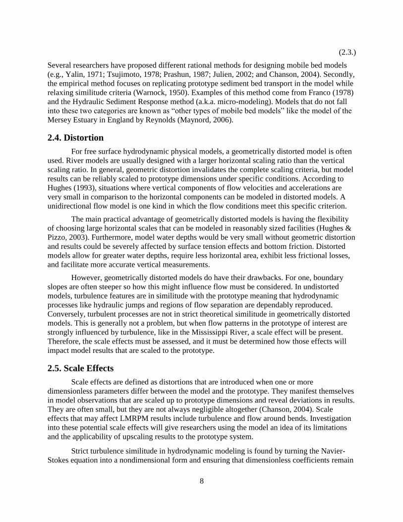
Figure 5.24. RM 128 High Flow Cross Sectional Velocity Profile. ............................................. 46
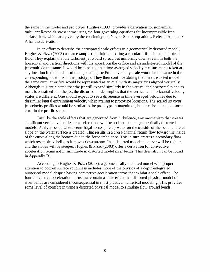
Figure 5.25. RM 107 Low Flow Cross Sectional Velocity Profile. .............................................. 46
Figure 5.26. RM 107 Medium Flow Cross Sectional Velocity Profile. ....................................... 46
Figure 5.27. RM 107 High Flow Cross Sectional Velocity Profile. ............................................. 47
Figure 5.28. RM 104 Low Flow Cross Sectional Velocity Profile. .............................................. 47
Figure 5.29. RM 104 Medium Flow Cross Sectional Velocity Profile. ....................................... 47
Figure 5.30. RM 104 High Flow Cross Sectional Velocity Profile. ............................................. 48
Figure 5.31. RM 61 Low Flow Cross Sectional Velocity Profile. ................................................ 48

viii
Figure 5.32. RM 61 Medium Flow Cross Sectional Velocity Profile. ......................................... 48
Figure 5.33. RM 61 High Flow Cross Sectional Velocity Profile. ............................................... 49
Figure 5.34. RM 59 Low Flow Cross Sectional Velocity Profile. ................................................ 49
Figure 5.35. RM 59 Medium Flow Cross Sectional Velocity Profile. ......................................... 49
Figure 5.36. RM 59 High Flow Cross Sectional Velocity Profile. ............................................... 50
Figure C.1. Experimental Setup at RM 130. ................................................................................. 63
Figure C.2. Experimental Setup at RM 128. ................................................................................. 63
Figure C.3. Experimental Setup at RM 107. ................................................................................. 64
Figure C.4. Experimental Setup at RM 104. ................................................................................. 64
Figure C.5. Experimental Setup at RM 61 .................................................................................... 64
Figure C.6. Experimental Setup at RM 59. ................................................................................... 65
Figure D.1. All Materials Used ..................................................................................................... 66
Figure D.2. Nikon Coolpix B500 Digital Camera. ....................................................................... 66
Figure D.3. McDoer 100 LED UV Flashlight. ............................................................................. 67
Figure D.4. 1.5 ft. (left) and 1.0 ft. (right) Tripods. ...................................................................... 67
Figure D.5. Ruler and Caliper. ...................................................................................................... 67
Figure D.6. UV Reactive Water Dye and Syringe. ....................................................................... 68
Figure D.7. Mariotte Bottles. ........................................................................................................ 68
Figure D.8. Green Water Based Acrylic Glow in the Dark Paint. ................................................ 68
Figure D.9. HDPE Painted PIV Particles...................................................................................... 69
Figure D.10. Corona Stainless Steel Scoop Hand Shovel. ........................................................... 69
Figure D.11. Nylon Aquarium Fishing Nets. ................................................................................ 69

ix
Abstract
The submergence of coastal wetlands in south Louisiana leaves communities, commerce,
industry, and ecosystems vulnerable to extreme weather events and human and natural disasters.
The state of Louisiana has developed a plan to mitigate coastal land loss and with the help of
Louisiana State University and the Lower Mississippi River Physical Model, projects like large
scale sediment diversions will be extensively tested and researched to ensure proper
implementation and operation. Due to scaling and distortion of the physical model, complete
similitude with its prototype is not expected and scale effects are anticipated to affect the
hydrodynamics and, as a result, complete replication of sediment transport dynamics. The
objective of this study is to qualitatively and quantitatively observe and analyze the
hydrodynamics and hydraulics in a geometrically distorted river model by utilizing two flow
visualization techniques - dye injection to investigate the assumption of Reynolds
independence and particle image velocimetry (PIV) to investigate the impact of model distortion
on 2-dimensional hydrodynamics. The results of the studies effectively answer the questions
raised in the objective of this thesis. Dye injection studies show increasing levels of mixing and
that 3-dimensional hydrodynamics are observable in the bends of the model river channel. Also,
PIV-measured surface velocities show good agreement with theoretical values. These results are
intended to help understand the limitations of the physical model so that the model results can be
properly applied and, if necessary, modifications to the model can be made to improve the
results. This understanding is critical to ensure that the results from this research tool are
properly used to aid in river management and coastal restoration planning, design, and policies
made by the Louisiana Coastal Protection and Restoration Authority.

1
Chapter 1. Introduction
Human intervention in the Mississippi River Drainage basin and in the river itself have
negatively affected the hydrology and hydraulics associated with the system. While this
intervention has promoted economic growth and protected communities adjacent to the river
from flooding, the downstream ecology of the Mississippi River Delta has faced the brunt of
those impacts. Freshwater and sediment starved wetlands are quickly transforming into open
water and receding into the Gulf of Mexico. The issue is further exacerbated by relative sea level
rise, making the need to protect the communities and industries that rely on those wetlands for
storm defense increasingly urgent. Louisiana’s Coastal Protection and Restoration Authority
(CPRA), the state agency responsible for implementing and enforcing coastal protection and
restoration projects, has developed a master plan for a sustainable coast and has identified large
scale sediment diversions as a top priority. In partnership with Louisiana State University (LSU),
CPRA has built a hydraulic, mobile bed physical model of the lower 195 miles of the Mississippi
River known as the Lower Mississippi River Physical Model (LMRPM). One of the key goals of
this model is to investigate the river’s response to river sediment diversions, relative sea level
rise, and future flow and sediment loads. The model was designed with a geometric distortion
and scaled to specific parameters in order to house it in a reasonably sized facility and to ensure
similarity with its prototype (the Mississippi River). Due to the distortion and scaling of the
model, scale effects are expected to impact some laboratory results. Scale effects arise when
force ratios are not identical between a model and its real-world prototype and result in
deviations between the up-scaled model and prototype observations. In an effort to explore the
anticipated scale effects in the LMRPM, flow visualization studies were conducted utilizing
techniques such as dye injection and particle image velocimetry (PIV). If the model is expected
to yield results that will aid in decision making related to sediment diversions and river
management, it is important to understand the model’s capabilities and limitations.
1.1. The Mississippi River Delta
Draining 41 percent of the 48 contiguous states of the United States, the Mississippi
River runs through the heart of the North American continent and empties into the Gulf of
Mexico. It has a watershed basin covering more than 1,245,000 square miles of land making it
the third largest drainage basin in the world (USACE, 2019). At and near its mouth lies Southern
Louisiana. Here, the “Mighty Mississippi” has formed a 9,650 square mile low gradient delta
plain known as the Mississippi River Delta plain (Blum & Roberts, 2012). It was built by regular
avulsion of the sediment rich river during the middle to late Holocene epoch (~ 7000-8000 yBP)
when most of the world’s large river deltas began to form as sea-level rise decelerated following
deglaciation from the last glacial period (Stanley & Warne, 1994). The Mississippi River Delta
represents a succession of river courses and five delta complexes that created the wetlands,
bayous, shallow bays, emergent ridges, and barrier islands that it comprises today (Figure 1.1.).
Natural deltas are dynamic and exist in a state of constant change. However, the once wild
Mississippi River has been tamed and constricted by human activities for navigation and flood
control.

2
Figure 1.1. Holocene deltas (1,2,3,4, and 5) of the Lower Mississippi River. Figure obtained
from Blum & Roberts (2009).
Beginning in the twentieth-century, unprecedented levels of human activities in the
Mississippi River basin have unfavorably altered the hydraulics and natural course of the river.
Prior to anthropogenic influences, Blum & Roberts (2009) estimate the annual total suspended
sediment load in the lower river to be 400-500 MT (Million Tons) year-1. That sediment supply
has been reduced by 50% to 205 MT year-1. The construction of levees for flood protection,
dams for navigation, and land use changes within the drainage basin have all contributed to that
reduction. The current supply of sediment in lower river is less than the sediment trapping rate of
modern deltas (240-300 MT year-1) which is not enough to construct new land or sustain existing
land (Blum & Roberts, 2012). Furthermore, levees along the lower Mississippi River have
hydraulically isolated adjacent wetlands and disrupted their source of sediment distribution by
impeding avulsion and flooding. The results of these influences have turned much of the once
thriving marshes and wetlands into open water. Deprived of sediment minerals and nutrients,
they cannot accumulate enough land or biomass to compensate for eustatic sea-level rise as well
as natural and anthropogenic subsidence. In the last 80 years Louisiana has lost 1,900 square
miles of land (Figure 1.2.) and an additional 2,250 square miles are at risk of being lost in the
next 50 years according to CPRA (2017). The issue has become so serious that CPRA has called
it a coastal land loss crisis and actively works to heighten public awareness. It is a problem that
affects communities and industries alike and has far reaching consequences.

3
Figure 1.2. Historic Land-Water change from 1932-2010. Approximately 1,900 square miles.
Figure obtained from CPRA (2017).
The value of the Mississippi River Delta spans community, industry, economics, and
ecology. Coastal Louisiana is home to 2 million people, it facilitates the world’s largest port
complex, and is a haven for 5 million migratory waterfowl. Nationally, the region serves 20% of
waterborne commerce, 26% of commercial fisheries, and 25% of hydrocarbon production
(CPRA, 2017). Barrier Islands, marshes, and swamps along coastal Louisiana reduce storm surge
from storms and hurricanes while also playing a vital role in carbon and nitrogen cycling. The
continued loss of land in the delta could potentially increase the cost of annual flood damage by
ten times in the next 50 years if bold protection and restoration measures are not implemented
(CPRA, 2017).
1.2. Sediment Diversions
Submergence of coastal wetlands in the Mississippi River Delta cannot be entirely
avoided. A lack of sufficient sediment supplies in the lower river and the loss of its natural
processes due to engineering for navigation and flood control have made the delta vulnerable to
relative sea level rise. However, reestablishing hydraulic connectivity between the river and its
wetlands with sediment diversions could potentially mitigate land loss (Blum & Roberts, 2012).
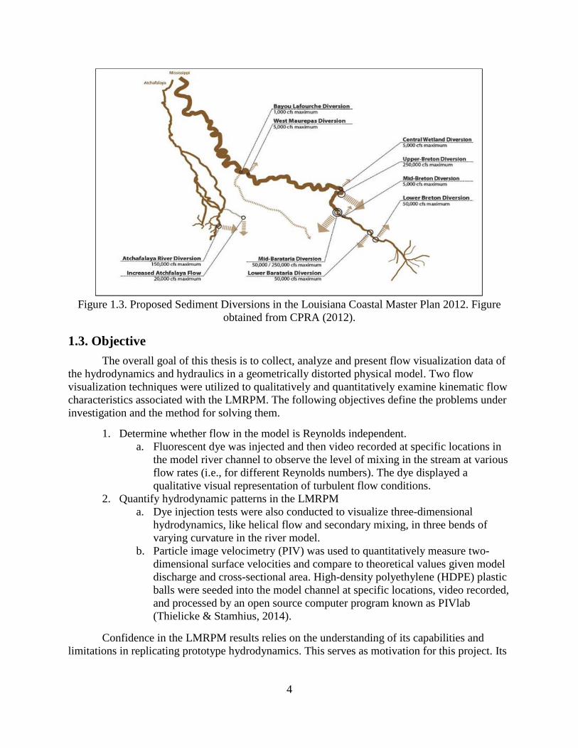
Louisiana’s Comprehensive Master Plan for a Sustainable Coast (CPRA, 2017) calls for the use
of land building and land sustaining sediment diversions to reintroduce river sediment to delta
plain wetlands (Figure 1.3.). Examples of delta growth at the mouth of the Atchafalaya River,
Wax Lake Delta, and Cubits Gap show the potential land building capacity of sediment
diversions and have evoked interest in their implementation along the Lower Mississippi River.
To test the land building capacity of these proposed sediment diversions, numerical modeling
can be used to simulate and quantify the results of diversion structures to optimize design and
ensure their success. Furthermore, these results can be coupled with the LMRPM to understand
how the river responds to these structures and how they impact dredging patterns, slopes and
stages, and river power.
4
Figure 1.3. Proposed Sediment Diversions in the Louisiana Coastal Master Plan 2012. Figure
obtained from CPRA (2012).
1.3. Objective
The overall goal of this thesis is to collect, analyze and present flow visualization data of
the hydrodynamics and hydraulics in a geometrically distorted physical model. Two flow
visualization techniques were utilized to qualitatively and quantitatively examine kinematic flow
characteristics associated with the LMRPM. The following objectives define the problems under
investigation and the method for solving them.
1. Determine whether flow in the model is Reynolds independent.
a. Fluorescent dye was injected and then video recorded at specific locations in
the model river channel to observe the level of mixing in the stream at various
flow rates (i.e., for different Reynolds numbers). The dye displayed a
qualitative visual representation of turbulent flow conditions.
2. Quantify hydrodynamic patterns in the LMRPM
a. Dye injection tests were also conducted to visualize three-dimensional
hydrodynamics, like helical flow and secondary mixing, in three bends of
varying curvature in the river model.
b. Particle image velocimetry (PIV) was used to quantitatively measure two-
dimensional surface velocities and compare to theoretical values given model
discharge and cross-sectional area. High-density polyethylene (HDPE) plastic
balls were seeded into the model channel at specific locations, video recorded,
and processed by an open source computer program known as PIVlab
(Thielicke & Stamhius, 2014).
Confidence in the LMRPM results relies on the understanding of its capabilities and
limitations in replicating prototype hydrodynamics. This serves as motivation for this project. Its

5
goal is to observe the scale effects associated with a geometrically distorted mobile-bed physical
river model.

6
Chapter 2. Physical Modeling
Due to the tremendous cost and scale of civil engineering projects, physical models are
commonly used during design stages to optimize structure and test prototype capabilities at a
reasonable laboratory scale (Chanson, 2004). Physical models of rivers have existed as early as
the 19th century when Louis Jerome Fargue built a model of the Garonne River at Bordeaux,
France. Since then, many researchers utilized these types of physical models proposing different
approaches to better replicate natural rivers (e.g., Einstein & Chien, 1956; Yalin, 1971; and
Parker, 1978). Physical river models allow the study of natural phenomenon under controlled
laboratory conditions to predict various scenarios at a low-cost relative to studies that can be
done in the field. The reason it is possible to model the hydrodynamic forces of rivers is because
there is an understanding of how to scale physical models. With one that is properly scaled,
measured and observed responses can be translated to full scale values (Hughes & Pizzo, 2003).
2.1. Similitude
In physical modeling the term similitude refers to the similarity of various characteristics
of the model to its prototype. Differentiation of prototype and model are usually given by
subscripts in order to calculate scale ratios. For example, λr = λ𝑝
λ𝑚, where subscript ‘p’ is for
prototype, ‘m’ is for model, and ‘r’ is for ratio. Complete replication of prototype conditions is
met when all three of the following criteria are in similitude (Hughes & Pizzo, 2003):
a. Geometric Similitude: Achieved when ratios of all corresponding linear
dimensions between prototype and model are the same (i.e., xr = yr = zr, where xr
is the downstream, yr is the lateral, and zr is the vertical ratio). Models that do not
meet these criteria are either distorted (i.e., yr ≠ zr) or tilted (i.e., xr ≠ zr) (Julien,
2002).
b. Kinematic Similitude: Achieved when the ratio between components of all
vectorial motions (i.e., velocity, acceleration, and kinematic viscosity) for the
prototype and model are always the same for all fluid particles. Models designed
to meet these criteria follow the Froude similitude criterion (i.e., Fr = 1).
c. Dynamic Similitude: Achieved when ratios of all vectorial forces (i.e., mass
density, specific weight, and dynamic viscosity) between the prototype and model
are always the same. Models that meet these criteria have the same Froude and
Reynolds number ratio.
These three similitude criterion are met reasonably well for all free-surface flows in coastal and
riverine environments by geometrically undistorted Froude-scaled models. However, undistorted
models become unfeasible when area restrictions limit the size of a laboratory, so geometrically
distorted models should be considered provided that the flow conditions meet the necessary
criteria (Hughes & Pizzo, 2003).
2.2. Scaling
In hydraulic physical modeling one must consider the dominant forces acting on a
prototype to determine how to scale its model. For open channel flow models of rivers and
floodplains, gravity is the predominant force driving the flow of water. Thus, Froude similitude
criterion is used to scale these models because it satisfies similarity in the ratio of inertial to

7
gravity forces. For fully enclosed or pipe flow where viscous forces dominate, the Reynolds
number similitude criterion is used because it satisfies similarity in the ratio of inertial to viscous
forces. The dimensionless equations of Froude and Reynolds number similitude criterion are
given respectively by Ettema et. al. (2000) as
𝐹𝑟 =𝑈
√𝑔𝐿
(2.1.)
and
𝑅𝑒 =𝑈𝐿
𝜈
(2.2.)
where
U = a reference velocity,
L = a reference length (i.e., depth, d),
g = gravity,
and ν = viscosity.
However, simultaneous satisfaction of the Froude (Frm = Frp) and Reynolds (Rem = Rep) scaling
criteria is impossible since water is typically used in both the model and prototype (Chanson,
2004). Since gravity is the predominant force and resistance to flow does not depend on
viscosity, in hydraulically rough conditions, one must scale according to Froude similitude and
relax the Reynolds number criterion while ensuring a rough turbulent regime.
2.3. Design
Two kinds of models exist in hydraulic modeling of rivers. Depending on the amount of
sediment transport exhibited by the prototype system, one may choose to use a rigid bed or a
mobile bed model. Rigid bed models are used when river flow conditions are not great enough to
transport sediment. Exact Froude similitude or Froude similitude for tilted models are used to
design these kinds of models (Julien, 2002). Mobile-bed physical models are used when there is
a significant level of sediment transport occurring in the river of interest. These models are a
small representation of a river that is adjusted to replicate its natural characteristics to solve
sedimentation problems (Franco, 1978).
For a model of the lower Mississippi River, a mobile bed physical model should be
chosen given the significant amount of sediment transport exhibited by the prototype. When
designing mobile bed physical models, there are two methodologies to consider. First, the
rational method emphasizes dimensionless similitude including Froude number and Shields
parameter. It is recommended to keep the distortion for these types of models as low as possible
(Maynord, 2006). Chanson (2004) recommends a distortion factor ranging from less than or
equal to 5-10 to ensure minimal scale effects. The equation for distortion is given below,
Ω =𝑦𝑟
𝑧𝑟
8
(2.3.)
Several researchers have proposed different rational methods for designing mobile bed models
(e.g., Yalin, 1971; Tsujimoto, 1978; Prashun, 1987; Julien, 2002; and Chanson, 2004). Secondly,
the empirical method focuses on replicating prototype sediment bed transport in the model while
relaxing similitude criteria (Warnock, 1950). Examples of this method come from Franco (1978)
and the Hydraulic Sediment Response method (a.k.a. micro-modeling). Models that do not fall
into these two categories are known as “other types of mobile bed models” like the model of the
Mersey Estuary in England by Reynolds (Maynord, 2006).
2.4. Distortion
For free surface hydrodynamic physical models, a geometrically distorted model is often
used. River models are usually designed with a larger horizontal scaling ratio than the vertical
scaling ratio. In general, geometric distortion invalidates the complete scaling criteria, but model
results can be reliably scaled to prototype dimensions under specific conditions. According to
Hughes (1993), situations where vertical components of flow velocities and accelerations are
very small in comparison to the horizontal components can be modeled in distorted models. A
unidirectional flow model is one kind in which the flow conditions meet this specific criterion.
The main practical advantage of geometrically distorted models is having the flexibility
of choosing large horizontal scales that can be modeled in reasonably sized facilities (Hughes &
Pizzo, 2003). Furthermore, model water depths would be very small without geometric distortion
and results could be severely affected by surface tension effects and bottom friction. Distorted
models allow for greater water depths, require less horizontal area, exhibit less frictional losses,
and facilitate more accurate vertical measurements.
However, geometrically distorted models do have their drawbacks. For one, boundary
slopes are often steeper so how this might influence flow must be considered. In undistorted
models, turbulence features are in similitude with the prototype meaning that hydrodynamic
processes like hydraulic jumps and regions of flow separation are dependably reproduced.
Conversely, turbulent processes are not in strict theoretical similitude in geometrically distorted
models. This is generally not a problem, but when flow patterns in the prototype of interest are
strongly influenced by turbulence, like in the Mississippi River, a scale effect will be present.
Therefore, the scale effects must be assessed, and it must be determined how those effects will
impact model results that are scaled to the prototype.
2.5. Scale Effects
Scale effects are defined as distortions that are introduced when one or more
dimensionless parameters differ between the model and the prototype. They manifest themselves
in model observations that are scaled up to prototype dimensions and reveal deviations in results.
They are often small, but they are not always negligible altogether (Chanson, 2004). Scale
effects that may affect LMRPM results include turbulence and flow around bends. Investigation
into these potential scale effects will give researchers using the model an idea of its limitations
and the applicability of upscaling results to the prototype system.
Strict turbulence similitude in hydrodynamic modeling is found by turning the Navier-
Stokes equation into a nondimensional form and ensuring that dimensionless coefficients remain
9
the same in the model and prototype. Hughes (1993) provides a derivation for nonsimilar
turbulent Reynolds stress terms using the four governing equations for incompressible free
surface flow, which are given by the continuity and Navier-Stokes equations. Refer to Appendix
A for the derivation.
In an effort to describe the anticipated scale effects in a geometrically distorted model,
Hughes & Pizzo (2003) use an example of a fluid jet exiting a circular orifice into an ambient
fluid. They explain that the turbulent jet would spread out uniformly downstream in both the
horizontal and vertical directions with distance from the orifice and an undistorted model of the
jet would do the same. It would be expected that time-averaged velocity measurements taken at
any location in the model turbulent jet using the Froude velocity scale would be the same in the
corresponding locations in the prototype. They then continue stating that, in a distorted model,
the same circular orifice would be represented as an oval with its major axis aligned vertically.
Although it is anticipated that the jet will expand similarly in the vertical and horizontal plane as
mass is entrained into the jet, the distorted model implies that the vertical and horizontal velocity
scales are different. One should expect to see a difference in time averaged velocities due to
dissimilar lateral entrainment velocity when scaling to prototype locations. The scaled up cross
jet velocity profiles would be similar to the prototype in magnitude, but one should expect some
error in the profile shape.
Just like the scale effects that are generated from turbulence, any mechanism that creates
significant vertical velocities or accelerations will be problematic in geometrically distorted
models. At river bends where centrifugal forces pile up water on the outside of the bend, a lateral
slope on the water surface is created. This results in a cross-channel return flow toward the inside
of the curve along the bottom due to the force imbalance. This in turn creates a secondary flow
which resembles a helix as it moves downstream. In a distorted model the curve will be tighter,
and the slopes will be steeper. Hughes & Pizzo (2003) offer a derivation for convective
acceleration terms not in similitude in distorted model river bends. This derivation can be found
in Appendix B.
According to Hughes & Pizzo (2003), a geometrically distorted model with proper
attention to bottom surface roughness includes more of the physics of a depth-integrated
numerical model despite having convective acceleration terms that exhibit a scale effect. The
four convective acceleration terms that contain a scale effect in a distorted physical model of
river bends are considered inconsequential in most practical numerical modeling. This provides
some level of comfort in using a distorted physical model to simulate flow around bends.

10
Chapter 3. The Lower Mississippi River Physical Model
Located near the bank of the Mississippi River on Baton Rouge, Louisiana’s Water
Campus, the LSU Center for River Studies is home to the Lower Mississippi River Physical
Model (LMRPM) (Figure 3.1.). The river model is 10,000 square feet and based upon the
topography and bathymetry of 14,000 square miles of southeastern Louisiana, including the
Mississippi River. It is a geometrically distorted mobile bed physical model comprising the
lower 195 miles of the Mississippi River from Donaldsonville, Louisiana through the Head of
Passes and into the Gulf of Mexico. The LSU Center for River Studies is a collaborative
partnership between CPRA and LSU to showcase Louisiana’s working delta, coastal program,
and research dedicated to coastal restoration and river management. The primary research focus
of the center is to operate the LMRPM and investigate the river’s response to sediment
diversions, relative sea level rise, and future flow and sediment loads. The model utilizes water
and a lightweight sediment to replicate prototype hydraulics and bulk non-cohesive sediment
transport. Understanding how the model performs and its limitations is important for proper
interpretation of the model results in studying various management strategies in the Lower
Mississippi River.
Figure 3.1. The Lower Mississippi River Physical Model. Image obtained from lsu.edu/river.
The LMRPM is a continuation of the Small-Scale Physical Model (SSPM) designed by
SOGREAH Consultants (SOGREAH, 2004), a French company specializing in physical models
of rivers. The SSPM was a mobile bed physical model comprising the lower 60 miles of the
Mississippi River. It was operated by LSU in collaboration with the CPRA to investigate
management strategies and their effects on flood control, navigation, and coastal restoration.
The LMRPM design philosophy is a combination of the rational and empirical
methodologies discussed before. It follows the rational method by meeting the three
dimensionless similitude criteria of Froude, critical Shields parameter, and critical particle
Reynolds number. Likewise, it follows the empirical method by empirically calibrating
parameters such as sediment time scale and sediment discharge while relaxing the Reynolds
number criterion. This design ensures similitude for gravitational flow and that model sediment
will behave like prototype sand.
3.1. Geometric Scaling
The geometric scale of the LMRPM was selected by two factors: a large domain and
minimum model Reynolds number (Rem) for turbulent conditions (i.e., Rem > 2000 for turbulent
conditions and Rem > 10,000 for fully turbulent conditions). Several geometric scales were

11
proposed and considered for design (Table 3.1.) (BCG Engineering & Consulting, Inc., 2015).
Ultimately a horizontal and vertical scale of 6,000 and 400 were chosen respectively. These
scales provide an appropriate model size and ensures a high enough Reynolds number for
sediment transport at required discharges (e.g., medium and large). However, these dimensions
also give the model a distortion level of 15, which exceeds the distortion recommended by Julien
(2002), Chanson (2004), and Shen (2012) for rational methods (i.e., 𝑦𝑟
𝑧𝑟=
6000
400= 15 > 5 − 10).
Table 3.1. Proposed LMRPM Geometric Scales.
Discharge (cfs) Zr Xr Distortion Rep Rem
400,000 500 12,000 24 457,000,000 2,243
1,350,000 500 12,000 24 1,540,000,000 7,570
400,000 600 12,000 20 457,000,000 1,845
1,350,000 600 12,000 20 1,540,000,000 6,228
400,000 500 9,000 18 457,000,000 2,528
1,350,000 500 9,000 18 1,540,000,000 8,533
400,000 600 9,000 15 457,000,000 2,054
1,350,000 600 9,000 15 1,540,000,000 6,933
400,000 400 6,000 15 457,000,000 3,774
1,350,000 400 6,000 15 1,540,000,000 12,736
400,000 500 6,000 12 457,000,000 2,897
1,350,000 500 6,000 12 1,540,000,000 9,777
400,000 600 6,000 10 457,000,000 2,316
1,350,000 600 6,000 10 1,540,000,000 7,818
Rep = prototype Reynolds number, Rem = model Reynolds number
3.2. Dynamic Scaling
There are two criteria most important for selecting the dynamic scale in a mobile bed
physical river model. They are the Froude and Reynolds number criterion and simultaneous
similitude of both parameters is impossible to achieve when the river model uses the same fluid
as the prototype (i.e., water). For river models, it is recommended that the model is scaled to
meet Froude similitude while relaxing Reynolds number similitude (Green, 2014) - the LMRPM
was designed following this guidance. Reynolds number relaxation is allowed because turbulent
and laminar channels are governed by the same dynamics using the same dimensionless
equations (Graveleau et al., 2011). From Froude similitude (Equation 2.1.), the velocity ratio and
water discharge ratio for the model were calculated and the equations are given respectively by:
𝑉𝑟 = √𝑧𝑟

12
(3.1.)
and
𝑄𝑟 = 𝑧𝑟3 2⁄ 𝑥𝑟
(3.2.)
From these equations we get the model velocity and discharge ratios of Vr = 20 and
Qr = 48,000,000.
3.3. Model Sediment Scaling
Model sediment was chosen based on the similarity of the critical particle Reynolds
number and the critical Shields parameter. By setting the critical particle Reynolds number
(Rec*) ratio (Equation 3.3.) and the critical Shields parameter (τc*) ratio (Equation 3.4.) to unity,
the size of the model sediment can be scaled as a function of the prototype diameter and the
specific gravity ratio. The material that was chosen is a ground unexpanded polystyrene with a
specific gravity of 1.05 g/cm3, which is a widely used lightweight sediment in physical modeling
(Frostick et al., 2011). Mississippi River sand has a specific gravity of 2.65 g/cm3 for
comparison. The model sediment can be scaled using Equation 3.5.
(𝑅𝑒𝑐∗)𝑟 =(𝑢∗)𝑟𝑑𝑟
𝜈
(3.3.)
(𝜏𝑐∗)𝑟 =(𝑢∗)𝑟
2
𝑔(𝑆𝑟 − 1)𝑑𝑟
(3.4.)
𝑑𝑚 = 3.2𝑑𝑝
(3.5.)
where
(u*)r = shear velocity ratio,
dr = particle diameter ratio,
ν = kinematic viscosity,
g = gravity,
and Sr = ratio of densities of particle and water,
Sediment in the Mississippi River changes seasonally depending whether the flow is high
or low. From a survey conducted near Belle Chase, Louisiana in 2015, it was found that
sediment in the lower river is composed mainly of very fine to fine sand (BCG Engineering &
Consulting, Inc., 2015). The model sediment distribution was properly scaled using Equation 3.5.
and is summarized in Table 3.2.

13
Table 3.2. Design Characteristic Sediment Sizes for Both Prototype and Model (BCG
Engineering & Consulting, Inc., 2015).
Type D10 (mm) D50 (mm) D90 (mm)
Prototype (Mississippi) 0.08 0.12-0.14 0.25
Model 0.25 0.40-0.45 0.80
3.4. Time Scaling
There are two main time scales that the model was designed for. First is the hydraulic
time scale ratio, which is based on Froude similitude and is given by:
𝑇𝑟 =𝑥𝑟
√𝑧𝑟
(3.6.)
Second is the sediment time scale. The sediment time scale was calculated based on previous
studies conducted by SOGREAH Consultants. They proposed a sediment time scale based on a
similarity law that resulted from a study of the Seine Estuary as a function of the hydraulic time
scale and the sediment specific gravity ratio:
𝑇𝑠𝑟 = 𝑇𝑟(𝛾𝑠 − 1)𝑟
(3.7.)
From these equations we get the model times scales of Tr = 300 and Tsr = 9900. However, a
sediment time scale of 6600 was ultimately selected from empirical calibration on the LMRPM
conducted by Hooper (2019).
3.5. LMRPM Scale Ratio Summary
The specific scale ratios for the LMRPM are as follows:
1. Horizontal Scale Ratio:
Xr = 1:6,000 (for channel width and length)
2. Vertical Scale Ratio:
Zr = 1:400 (for water depth, dune height and length)
3. Distortion Factor Ratio, as given by equation 2.3.:
Ω = 6000
400 = 15
4. Velocity Scale Ratio, as given by Equation 3.1.:

14
Vr = 1:√400 = 1:20 (for channel flow velocities)
5. Discharge Scale Ratio, as given by Equation 3.2.:
Qr = 1:6,000*4003/2 = 1: 48,000,000
6. Hydraulic Time Scale Ratio, as given by Equation 3.6.:
Tr = 1:6000
√400 = 1:300
7. Sediment Transport Time Scale Ratio, as given by Hooper (2019):
Tsr = 1:6600
8. Sediment Size Scale Ratio is given by Equation 3.5. and summarized in Table 3.2.

15
Chapter 4. Qualitative Flow Visualization Studies Via Dye Injection
Flow visualization is one of many experimental tools that are utilized to measure the flow
of fluids which are typically transparent and invisible to the naked eye. Flow patterns can be
made visible by applying flow visualization methods which can be observed directly or recorded
with a video camera. At a specific instant in time, information on the flow is available for the
whole field of view. This observed information can either be qualitative or quantitative.
Qualitative information allows for interpretation of the mechanical and physical processes
involved in the development of the flow (Merzkirch, 1987).
One of the basic principles of flow visualization is to observe light scattered from either
fluid molecules or tracer particles. Due to the extremely weak scattering of light from fluid
molecules, flows are often seeded with small tracer particles (e.g., microspheres, smoke, or dye)
to capture more intense radiation scattered from these tracers. Scattered light carries information
on the state of the flow at the position of the particle. Thus, it is assumed that the motion of the
tracer is the same as the motion of the fluid. However, Merzkirch, 1987 states that this
assumption doesn’t always hold true for unsteady flows. Flow visualization by observing the
scattering light from smoke or dye is mainly a qualitative method (Merzkirch, 1987). For this
research, dye injection studies were conducted in order to explore Reynolds independence in the
LMRPM. Qualitative information was extracted from the visualization of mixing for an
increasing range of flow conditions. Furthermore, information in the bends and crossings of the
river model were interpreted for quality and similarity to expected prototype behavior to ensure
reliable flow and sediment transport in the model.
4.1. Materials
The materials that were used for qualitative flow visualization studies via dye injection
were chosen with consideration given to methodological applications from Merzkirch (1987) and
issues of concern from Miau et. al. (1990), Lin et. al. (1993), and Holden (2005). To improve
results from light scattering, the signal to noise ratio can be reduced if the tracer can emit its own
light rather than scattering incident light (Merzkirch, 1987). This principle is realized by
fluorescent or phosphorescent tracers which emit light when induced by incident radiation with
the appropriate wavelength. From this information, fluorescent tracers and an ultraviolet lighting
source were chosen to be used for all flow visualization studies.
For dye injection, a Green UV Reactive Water Dye (Figure D.6. in Appendix D) was
used to visualize turbulent mixing. Three one-ounce bottles of the concentrated product were
purchased from a company known as GLO Effex. Merzkirch (1987) suggests using tracers with
neutral buoyancy to ensure a reliable match with the motion of the working fluid. To address
this, thirty drops of the concentrated dye was mixed with 200 mL of water to give the tracer a
density of 1.05 g/cm3. The working fluid is a mixture of water with a 0.44% concentration of
surfactant and a 0.03% concentration of pool shock, giving the mixture a density of 1.07 g/cm3.
Density of the two fluids was calculated by measuring the weight of an empty beaker and the
weight of a beaker filled with 200 mL of each fluid. The empty beaker weight was subtracted
from the full beaker weight and divided by the volume of the fluid.
Injection velocity is another consideration for reliable imitation of the flow by a dye
tracer. The velocity of the dye tracer should either match or be smaller but comparable to the
flow velocity of the working fluid to minimize disturbance (Lin et. al., 1993). Another issue of

16
concern is disturbance introduced by the dye injection tube. To address these issues, it was
decided to use a series of Mariotte bottles to inject dye through the cross section of the channel.
A Mariotte bottle is a device that allows a constant flow of fluid from a container (Holden,
2005). It consists of a bottle with an injection tube and a vent tube that allows air bubbles to be
drawn into the bottle to equalize pressure and provide a constant flow. For this research, a series
of Mariotte bottles were constructed to meet the specific needs of these studies. A pack of 12
Dynalon 5 oz. standard spout non-vented narrow mouth wash bottles were purchased from
Grainger Industrial Supply. A hole was drilled into the bottom of 9 of the bottles and a plastic
tube that is included with the bottle was placed in the hole to act as a vent tube. Three devices,
each made with a series of three bottles and held together with zip ties, were made (Figure D.7.
in Appendix D). The three bottles were placed on wooden rods and held upside down so that
they could sit over the channel on top of the model levees to inject dye. Refer to Figures C.1. –
C.6. in Appendix C for a visual depiction.
An integral part to flow visualization is lighting. A proper lighting system will optimize
the information that can be interpreted from observations or recording of tracer seeding. To
excite the dye tracer to emit its own light, an ultraviolet light source was used. A McDoer 100
LED UV Flashlight was purchased from Amazon.com and placed on a 1.5 ft. high tripod
adjacent to the regions of interest for illumination (Figure D.3. and D.4. in Appendix D). The
LED UV flashlight has an 18 W, 385-395 nm ultraviolet radiation wavelength, which is enough
to induce radiation in the fluorescent dye tracer.
The fundamental piece of equipment for recording flow visualization observations is a
camera. For these studies a Nikon Coolpix B500 digital camera was used to video record the
tracer seeded flow (Figure D.2. in Appendix D). The camera can record videos in Full HD, a
1920 x 1080-pixel format, which offers high quality video imaging for a digital camera. It was
mounted on a 1 ft. high tripod adjacent to the regions of interest to capture portrait-oriented
images (flow traveling from left to right).
4.2. Methods
For this research, it was decided to observe dye injection studies at three locations, two
cross sections at each location, and four different flows at each cross section. The three locations
are near water level gages on the model which are labeled as Bonnet Carré North, Carrolton, and
Alliance. The gages on the model coincide with US Army Corps of Engineers (USACE) gages in
the prototype. The two former locations were chosen to coincide with numerical modeling
research for depth averaged and surface velocities in the Mississippi River at the same locations
to be analyzed and compared to this research at a later date. The latter location was chosen due to
its importance in the model and in the prototype. Alliance is located near the proposed Mid-
Barataria Sediment Diversion which is a critical structure in the CPRA Coastal Master Plan, and
the research conducted at the LSU Center for River Studies. Refer to Figure 4.1. for spatial
context of the locations.

17
Figure 4.1. Model Domain with USACE Gages Near Experimental Locations. Image Source:
ESRI, DigitalGlobe, GeoEye, Earthstar Geographics, CNES/Airbus, USDA, USGS, AeroGRID,
IGN, and the GIS User Community.
At each location, two cross sections were chosen to observe dye tracers in the model
channel. One bend and one crossing at each location were chosen to give insight into how flow
in these physical features are simulated in the distorted model. River miles (RM) 130 and 128
were chosen and are located near the Bonnet Carré North gage (Figure 4.2.). They are situated in
the bend before and in the crossing after the gage respectively. The Bonnet Carré Spillway is a
critical structure for flood control in the real world, so understanding how flow passes before and
in front of the model structure is valuable information for model operation. RM 107 and 104
were chosen and are located near the Carrolton gage just before the City of New Orleans (Figure
4.3.). They are situated in the crossing and the bend before the gage respectively. RM 61 and 59
were chosen and are located near the Alliance gage (Figure 4.4.). They are situated in the
crossing before and the bend after the Mid-Barataria Sediment Diversion structure respectively.
Understanding how flow passes before and after a sediment diversion structure is of critical
value for the success of the LMRPM. Furthermore, the proximity of each cross section to a gage
provided a water level measurement for cross sectional area and ultimately Reynolds number to
be calculated for analysis of the observed data.

18
Figure 4.2. Bonnet Carré North Locations. RM 130 and 128.
Figure 4.3. Carrolton Locations. RM 107 and 104.
Figure 4.4. Alliance Locations. RM 61 and 59.
RM
128

19
Finally, four flows were observed at each cross section in order to visualize mixing for an
increasing level of turbulence. For this research, turbulent flow is assumed to be achieved at a
Reynolds number (Equation 2.2.) greater than 2000 (Chow, 1959). The four chosen flows begin
with a very low flow of 3 gpm, then a low flow of 4.6 – 5.0 gpm (equivalent to 490,000 –
530,000 cfs in the prototype), a medium flow of 6.7 – 6.9 gpm (710,000 – 740,000 cfs in
prototype), and lastly a high flow of 9.4 – 9.8 gpm (1,000,000 – 1,050,000 cfs in prototype). The
very low flow was controlled at an unfluctuating state which was pumped from the head box of
the model. A range of flows from low to high were observed due to a hydrograph that was being
run through the model. The hydrograph was chosen to be observed because it is a typical
hydrograph that is consistently pumped into the LMRPM and would give insight into typical
turbulence levels encountered in the model. Only flows at or above 3 gpm are modeled in the
physical model. This flowrate equates to 400,000 cfs in the prototype, which CPRA proposes
sediment diversions to be operated at or above this minimum. For this reasoning, it was decided
to observe the flowrates described above.
4.3. Procedures
Procedural methods for the dye injection experiments consisted of video recording dye
tracers, calculating Reynolds numbers, and video editing to extract as much information as
possible. First, bed measurements were taken before the hydrograph was run through the model
and again after at cross sections where sediment was present. The only cross sections that had
sediment were RM 128 and 107. Measurements were taken with a ruler and caliper. The ruler
measured distance across the channel and the caliper was lowered to the height of the sediment
bed to measure depth. Caliper precision is ± 2 mm. This was done to calculate cross sectional
area.
Next, 10 mL of dye tracer was injected into the vent tube of each of the three Mariotte
bottles with a syringe. All the lights in the model warehouse were turned off and the LED UV
flashlight was turned on to illuminate the region of interest. This was done to allow for proper
lighting of the fluorescent dye. When the desired flow was reached, a determined amount of
travel time for flow to reach the region of interest was allowed to pass. Travel times were
deduced from analyzing previous hydrograph results. By looking at the time difference of a
discharge change and stage change, travel times were determined. Once that time had passed, the
camera began recording video and the bottles were flipped to allow the dye tracer to seed the
flow at a specific distance from the region of interest. Cross sections at RM 130, 128, 107, and
61 were seeded at 12 cm from the cross section to the tip of the injection tube. RM 104 and 59
were seeded at 16 cm due to their location at the end of bends in the model river. A sufficient
distance was required to allow the dye to flow naturally around the bend, otherwise it was
observed that the dye would flow straight into the wall. Furthermore, the dye was injected at a
depth of 1.5 – 3 cm below the water surface depending on how high the stage was. The time of
injection was also recorded in order to reference flowrate and stage height which is recorded by
the model control software.
Once all the desired flows and locations were observed, the videos were uploaded to a
computer to be processed. Video processing of the observations were done through a processing
program known as VideoPad Video Editor which is developed by NCH Software®. This
program was used to cut the videos to an appropriate length and remove any frames without dye.
The videos were edited for consistent orientation and enhanced for improved image quality.

20
Videos of observations at RM 104, 61, and 59 were flipped 180º because they were recorded
from the east bank of the model river, where as the rest of the videos were recorded from the
west bank. This was done to capture a consistent frame orientation (water flowing from left to
right). These locations were filmed from the east bank because of interference from a sharp bend
(RM 104) and the Mid-Barataria Sediment Diversion structure (RM 61 and 59) on the west bank
of the cross section. Refer to Figures C.1. – C.6. in Appendix C for experimental set up images.
Once the videos were cut and properly oriented, three video effects were uniformly
applied to improve image quality using VideoPad Video Editor by NCH Software ©. Each video
was sharpened to a value of 25.00 out of 50.00. Color adjustments were applied and include no
changes to the brightness (brightness number 0.00 from a range of -255.00 to 255.00), increasing
contrast to a value of 20.00 out of 100.00, and increasing gamma to 1.00 out of 5.00. Lastly, the
exposure was decreased to -0.20 from a range of -1.00 to 1.00. After enhancement, the shortened
videos were saved and 30 frames per second were extracted. The videos and images were then
analyzed for qualitative analysis.
In order to describe the level of turbulence that was observed, Reynolds number for each
flow was calculated at each cross section. Model designed cross sections were obtained from
Ardurra Group and digitized using a software program called WebPlotDigitizer ©. Digitized
cross sections were then converted to distorted model scales and used to calculate cross sectional
area and wetted perimeter which led to a calculation of Reynolds number. Here, Reynolds
number is defined as:
𝑅𝑒 = 𝑉𝑅ℎ
𝜈
(4.1.)
where V is average velocity,
𝑉 =𝑄
𝐴𝑐
(4.2.)
Rh is hydraulic radius,
𝑅ℎ =4𝐴𝑐
𝑝
(4.3.)
ν is kinematic viscosity which is 1.004 *10-6 m2/s at 68º F (Chow, 1959), which is the
experimental temperature of the water. Q is discharge from the head box. Ac is cross sectional
area and p is wetted perimeter. Ac and p were calculated from the digitized cross sections, bed
measurements taken before and after each run, and stage height at the time of observation.
4.4. Results
In Figures 4.5. – 4.28, one frame from each observation is presented along with its
corresponding Reynolds number described beneath each image. The presented images have been

21
edited as previously described. Furthermore, the same frame number for each cut video (Frame
no. 100) was chosen to capture a consistent time of seeding for each observation. Due to the
possibility that each video was not cut uniformly for all observations, the timing for each
presented frame may be slightly different. However, timing differences would be less than 1
second between all observations, so confidence in timing is high. For RM 128 and 107 where
sediment was present and bed measurements were taken, the very low flow and low flow cross-
sectional areas were calculated with measurements taken before the run, high flows with
measurements taken after the run, and medium flows with the average between the before and
after measurements. This was done to capture bed morphology during the run assuming that
most sediment transport takes place on the rising limb of the hydrograph, which is when all the
observations were captured.
Some general observations were made for each video which serve as qualitative data for
the dye injection experiments. In Figures 4.5. – 4.8., RM 130 represents a typical bend of about
90º. In each successive video, flow speeds and mixing get progressively higher with increasing
flow rates. The plumes of dye became progressively narrower and less definable. Higher levels
of mixing are observed when the definition of the dye begins to decrease. This can be seen in the
still frames but is more apparent when analyzing the videos. The flow appeared to hit the wall
and hug the outside of the bend further away from the injection point with increasing flow rates
and some helical flow or secondary mixing was observable after contact with the wall. Lighting
became less than ideal as flow rates increased due to the presence of the black sediment which
scattered less light and resulted in a darker image.
Figure 4.5. RM 130 Very Low Flow. Re = 3156.

22
Figure 4.6. RM 130 Low Flow. Re = 5139.
Figure 4.7. RM 130 Medium Flow. Re = 6796.
Figure 4.8. RM 130 High Flow. Re = 8843.

23
Figures 4.9. – 4.12. at RM 128 had some of the highest quality imaging of all the
locations. This is due to the amount of sediment on the bed. There is enough to contrast the
fluorescent dye and not too much to reduce the scattering of the ultraviolet light. Flow speeds
and levels of mixing appeared to get higher with increasing flow rates. The plumes didn’t narrow
as much as they did at other locations, but they became more scattered as flow rates increased.
Overall the lighting was good for each observation. However, the lighting for the high flow was
not great, but was still adequate to extract information.
Figure 4.9. RM 128 Very Low Flow. Re = 3500.
Figure 4.10. RM 128 Low Flow. Re = 5480.

24
Figure 4.11. RM 128 Medium Flow. Re = 7352.
Figure 4.12. RM 128 High Flow. Re = 9550.

25
At RM 107 (Figures 4.13. – 4.16.) the lighting was less than ideal for all the observations.
This is due to the significant amount of sediment on the bed, which reduces ultraviolet light
scattering. The injection point could not be seen in any of the videos. However, enough
information was extracted. Dye plumes moved progressively faster, became narrower, more
mixed, and less definable with increasing flow rates.
Figure 4.13. RM 107 Very Low Flow. Re = 3417.
Figure 4.14. RM 107 Low Flow. Re = 5389.

26
Figure 4.15. RM 107 Medium Flow. Re = 7482.
Figure 4.16. RM 107 High Flow. Re = 11224.

27
At RM 104 (Figures 4.17. – 4.20.) is the sharpest bend of all the observed locations. Here
plumes appeared to increase in speeds, levels of mixing, and decreasing in definition with
increased flow rates. The dye flowed towards the wall and along the outside of the bend, but to a
decreasing extent with increasing flow rates. Increasing levels of helical flow or secondary
mixing was easily observable at this bend compared to others.
Figure 4.17. RM 104 Very Low Flow. Re = 2551.
Figure 4.18. RM 104 Low Flow. Re = 4051.

28
Figure 4.19. RM 104 Medium Flow. Re = 5652.
Figure 4.20. RM 104 High Flow. Re = 7589.

29
At RM 61 (Figures 4.21. – 4.24.) dye plumes moved very quickly and became
progressively narrower. The definition didn’t change as significantly as in other locations and
neither did the mixing. This is likely due to the spatial context of the location. It is in a relatively
straight portion of the river. There are no relatively sharp bends upstream and a very gentle bend
just downstream. Also, the outside plumes didn’t flow as much as the middle plume at higher
flow rates. This is due to an issue with the Mariotte bottles not properly injecting dye.
Figure 4.21. RM 61 Very Low Flow. Re = 3176.
Figure 4.22. RM 61 Low Flow. Re = 5103.

30
Figure 4.23. RM 61 Medium Flow. Re = 7011.
Figure 4.24. RM 61 High Flow. Re = 9771.

31
RM 59 (Figures 4.25. – 4.28.) is located in a very gentle bend. The plumes of dye didn’t
hit the wall until the very end of the bend and tended to flow more with the curve as compared to
other bends where dye would hit the wall. Slow plumes speeds, increasing levels of mixing, and
decreasing dye definition were observed. Helical flow and secondary mixing were not as
apparent. This location had the poorest lighting. No information was able to be extracted for the
high flow rate because of poor lighting.
Figure 4.25. RM 59 Very Low Flow. Re = 2546.
Figure 4.26. RM 59 Low Flow. Re = 3885.

32
Figure 4.27. RM 59 Medium Flow. Re = 5407.
Figure 4.28. RM 59 High Flow. Re = 6967.
4.5. Discussion
From all of the locations and flowrates, the same general observations occurred and were
consistent. Flow visualization via dye injection provided a non-destructive way of observing
some of the complex hydrodynamics and levels of mixing. The plumes would narrow, and
definition would decrease with higher flows (i.e., higher Reynolds numbers). Perhaps the
occurrence of narrowing dye plumes could be attributed to the scale effects previously
mentioned. However, without further investigation that cannot be stated for certain. A clear
change in the level of mixing at different flowrates in different cross sections was also
observable. Due to the varying geometry of the channel bed, it was apparent that a greater
difference in mixing would occur at different flow rates. The most significant change in the
definition and scatter of the dye occurred from the medium to high flow in RM 130, 107, 104,
and 61. At RM 128 the most significant change in definition occurred from low to medium and a
significant change in scatter occurred from medium to high. At RM 59, the most significant
change occurred in definition and scatter occurred from low to medium flows. This observation
suggests that geometry has an impact on the mixing in the model channel. Overall, the results of

33
these observations satisfy the objective of this thesis to observe levels of mixing in the model
channel to examine Reynolds independence.
In the bends, the plumes would flow into the walls sooner and hug the outside banks of
the curve with increasing sharpness of curvature. Helical flow and secondary mixing were more
easily observable in sharper bends as well. Narrowing of the dye plumes and decreasing levels of
definition were consistent in the bends as they were in the crossings. Again, the results of these
observations satisfy the objective to visualize three-dimensional hydrodynamics, like helical
flow and secondary mixing.

34
Chapter 5. Quantitative Flow Visualization Studies Via Particle Image
Velocimetry
When flow velocity information is desired, quantitative methods of flow visualization can
be utilized to identify the motion of individual tracers (Merzkirch, 1987). Imaging techniques
like particle tracking velocimetry (PTV), where individual particles are tracked between
successive images, and particle image velocimetry (PIV), where a group of particles are
identified in successive images, can capture two- and three-dimensional flow measurements for
laboratory scale fluids experiments. Conventional PIV systems consist of tracer particle seeding,
illumination, video recording, and image processing. PIV is an appealing technique due its
inherent simplicity, relatively low cost, and non-intrusiveness. Although instruments like
acoustic Doppler velocimeters (ADV) can provide quick and accurate velocity measurements,
contact with the flow is required and the equipment is relatively expensive to purchase and
operate. Furthermore, ADVs can only measure local velocities, whereas PIV can capture
instantaneous velocity at a large number of points at once on the water surface. The PIV concept
involves seeding flow with tracer particles that accurately follow fluid movement. Then, images
from the regions of interest are recorded and processed to calculate velocity by dividing particle
displacement by the time interval between successive frames.
5.1. Materials
Flows are visualized by a distribution of particles on the surface of the water using PIV
(Raffel et. al., 2007). The materials used for PIV studies in this research were similar in concept
to those used in the dye injection studies. Fluorescent tracers and UV light were utilized to
visualize flow which were video recorded, processed, and analyzed. Muste et. al. (2004) suggests
using particles that are neutrally buoyant and contrast background colors. This was addressed by
coating light weight particles with fluorescent paint. Nine hundred white HDPE plastic balls with
5/32 in. diameter and 0.95 g/cm3 density were purchased from Precision Plastic Ball Company
(Figure D.9. in Appendix D). Furthermore, two 2 oz. bottles of a green water based acrylic glow
in the dark paint was purchased from GloNation (Figure D.8. in Appendix D). For seeding, a
Corona stainless steel scoop hand shovel was used (Figure D.10. in Appendix D). For
illumination and recording, the same UV flashlight/tripod and digital camera/tripod assemblies
used for dye injection were employed. Lastly, 4 nylon aquarium fishing nets were purchased
from Amazon.com to be used for collecting particles downstream of the test section (Figure
D.11. in Appendix D).
5.2. Methods
The same locations and cross sections that were studied for dye injection were also
studied to measure surface velocities. RM 130 and 128 were observed near the Bonnet Carré
North gage, RM 107 and 104 were observed near the Carrolton gage, and RM 61 and 59 were
observed near the Alliance gage. However, three flow rates were observed at each cross section
rather than four. The three chosen flows coincide with the low, medium and high flows observed
in the dye injection studies. Low flows ranged from 4.6 – 5.0 gpm (490,000 – 530,000 cfs in
prototype), medium flows from 6.7 – 6.9 gpm (710,000 – 740,000 cfs in prototype), and high
flows from 9.4 – 9.8 gpm (1,000,000 – 1,050,000 cfs in prototype). Analyzed surface velocities
were then compared to theoretical values to measure for agreement. Refer to Figures 4.1. – 4.4.
for images of study locations.

35
5.3. Procedures
Procedural methods for the PIV experiments consisted of seeding and video recording
particle tracers, calculating theoretical surface velocities, and video and image processing to
calculate observed surface velocities. First, bed measurements were taken before and again after
the hydrograph for cross sections where sediment was present. RM 128 and 107 were the only
cross sections with sediment. Measurements were taken with a ruler and caliper to calculate
cross sectional area. Then, a reference distance across the channel was measured to be used in
the PIV program. This reference is an indention on top of the levees which marks every river
mile.
According to Sutarto (2015) the images produced by the camera must be clear, have good
contrast, and have no glare or shadow on the water surface. Quality imaging allows the PIV
software to detect the movement of particles on the water surface more accurately. These issues
were addressed by fluorescent particles, removing overhead lighting, and UV illumination. A
digital camera was placed adjacent to the channel on top of a 1 ft. tripod. The camera lens was
approximately 30 cm from the middle of the channel, it had a focal length of 4 mm (no zoom)
and was directed at a 10º angle. This is the acceptable limit for camera angle as suggested by
Kim (2006). A short distance and small angle ensure minimum image distortion for PIV analysis.
Refer to Figures C.1. – C.6. in Appendix C for experimental set up images.
Next when the desired flowrate was reached at the region of interest, the determined
travel time was allowed to pass. The camera then began recording and the particles were seeded
at a distance 35 cm away from the region of interest. According to Rafel et. al. (2007) a
homogeneous distribution of medium density is desired for high quality PIV recordings in order
to obtain optimal evaluation. To address this, 300 or 600 particles were seeded with a scoop
shovel allowing them to roll out as it was briskly moved back and forth across the channel. For
low flows 300 particles were seeded while 600 particles were seeded for the medium and high
flows. This was decided for the timing of the observation. With 300 at a low flow, there was a
good distribution for a sufficient period, whereas 600 gave a good distribution for a sufficient
period at medium and high flows. After the particles passed through the region of interest, the
particles were collected with fish nets.
Videos of the observations were then uploaded to a computer for processing and analysis.
VideoPad Video Editor and two GUI-based open sourced MATLAB toolboxes were utilized;
PTVlab and PIVlab. PTVlab was used to extract frames and convert them to black and white
images. However, the program only accepts .avi files so the videos had to be reformatted with
VideoPad Video Editor because they were recorded in a .mp4 format. Next, the processed
images were uploaded to PIVlab for analysis.
The following is a description of the procedure used for analyzing surface velocities in
PIVlab. The information comes from Thielicke & Stamhuis (2014) and personal experience with
the program. For the best results, it was found that using a sequence of frames starting and
ending with one that has a distribution of particles across the whole frame. A frame sequencing
style of 1-2, 2-3, 3-4, … was chosen for analysis when prompted to import images.
Next a series of analysis settings were applied. In the Analysis Settings tab, a region of
interest and a mask can be applied in the Exclusions (ROI, Mask) drop down option. A mask was
drawn around the area outside the region of interest to be excluded from analysis. The next drop-

36
down option is Image pre-processing where image enhancements can be made to improve
measurement quality. Contrast limited adaptive histogram equalization (CLAHE) is the first
enhancement option available to optimize regions of low and high exposure. This option was
enabled and a window size value of 200 pixels was chosen. An intensity highpass was enabled to
remove low frequency lighting and conserve high frequency information from the illuminated
particles. A filter size of 400 pixels was chosen. The last filter that was enabled was the intensity
capping filter which applies an upper limit of greyscale intensity and replaces any pixels which
exceeds the threshold. This works to reduce bias in non-uniform flows. The last drop-down
option in the tab is PIV settings where you can choose a cross correlation algorithm to derive the
most probable particle displacement in the interrogation areas. A single pass direct cross
correlation (DCC) and a multiple pass window deforming direct fast Fourier transform (FFT)
option is available. According to Huang et. al. (1997), DCC has shown to create more accurate
results but with the disadvantage of an increased computational cost. Despite its disadvantage,
DCC was chosen. It requires identifying an interrogation area and a step to increase vector
resolution. An interrogation area of 100 pixels was chosen to include a size that would contain at
least 10 particles, as suggested by Keane & Adrian (1993) and a step of 50 pixels was chosen.
In the next tab, Analysis, each frame can be analyzed. Vector creation and resolution can
be observed with each frame as the program analyzes every image. Upon completion of analysis,
results can be calibrated in the Calibration tab. Here a calibration image can be uploaded, and a
reference distance selected. A frame from each cross section was selected and the reference
distance that was previously recorded for each river mile was applied. A time step of 33.33 ms
was applied which correlates to the frame rate that the videos were recorded, and frames
extracted (30 frames per second).
Data validation is then completed in the Post processing tab. Here, erroneous vectors due
to poorly illuminated regions or strong out-of-plane flow can be removed and interpolated with
the Vector validation tool. Velocity limits can be chosen by checking the “display all frames in
scatterplot” box and clicking “Select velocity limits.” All the vectors are then displayed on a
scatter plot and a box can be drawn around the vectors that will be kept. Furthermore, a standard
of deviation filter was applied with a threshold of n=7. These validations were applied to all
frames and then reviewed. Interpolated vectors appear in orange and the sequence of images was
scanned to ensure quality data.
In the Plot tab and the Derive parameters/ modify data drop down, a velocity magnitude
parameter can be selected to display the velocity vector field for each image. Next a mean vector
frame can be calculated to display the mean velocity field by clicking “Calculate mean vectors.”
Data smoothing was applied to results to reduce noise. In the Modify plot appearance drop down
under the Plot tab, an HSV color map was applied to visualize velocity magnitudes. From the
mean velocity field frame, a velocity magnitude area mean value can be displayed from the
Parameters from area drop down under the Extractions tab by drawing a polygon around a
region of interest. Also extracted was surface velocity profiles across the channel at each cross
section. This was done for the same mean velocity field frame from the Parameters from a poly-
line drop down under the Extractions tab.
In order to determine if the experimental results calculated from PIVlab were reasonable,
theoretical surface velocities were calculated. Equation 4.2. was used to calculate the average
velocity in the cross section where discharge, Q, was taken as the flowrate through the head box

37
and cross-sectional area, Ac, was calculated from the digitized cross sections, bed measurements,
and water surface levels from model gages. Next, average surface velocities were calculated by
dividing average cross-sectional velocity by a surface velocity coefficient which is defined by
Marjang (2008). Surface velocity coefficients were determined by dividing the height of the
channel, H, by its width, B. The quotient of this ratio was then used to interpolate a value from
Table 5.1. Once the theoretical surface velocity was calculated it was compared to the
experimental results to determine if the observations were reasonable.
Table 5.1. Surface Velocity Coefficients Based on Channel Height to Width Ratio (Marjang,
2008, Table 8.).
H/B 0.25 0.30 0.40 0.50 0.60 0.70 0.80 0.90 1.00
coefficient 0.867 0.872 0.914 1.000 1.073 1.160 1.179 1.175 1.129
H/B 1.10 1.20 1.30 1.40 1.50 1.60 1.70 1.80 1.90
coefficient 1.120 1.102 1.089 1.085 1.080 1.076 1.088 1.087 1.095
5.4. Results
The results of the PIV studies are presented here in Figures 5.1. – 5.18 and Figures 5.19.
– 5.36. Figures 5.1. – 5.18. show the average cross-sectional surface velocity for each
observation which is labeled as “area mean value” in the image. Also displayed with each figure
is a small table with the calculated theoretical average cross-sectional surface velocity, the
observed average cross-sectional surface velocity, and the percent difference between them.
Figures 5.19. – 5.36. display the cross-sectional velocity profiles across each region of interest.
These results are extracted from the mean velocity field frame of the analyzed frames for each
observation. For RM 128 and 107 where sediment was present and bed measurements were
taken, the low flow cross-sectional areas were calculated with measurements taken before the
run, high flows with measurements after the run, and medium flows with the average
measurement between the two. This was done to capture the bed morphology throughout the run
assuming that most sediment transport takes place on the rising limb of the hydrograph which all
the observations were captured.

38
Figure 5.1. RM 130 Low Flow Average Cross Sectional Surface Velocity.
Figure 5.2. RM 130 Medium Flow Average Cross Sectional Surface Velocity.
Theo V_surf (m/s) 0.03709
Obs V_surf (m/s) 0.03507
% Diff 5.45
Theo V_surf (m/s) 0.04924
Obs V_surf (m/s) 0.03826
% Diff 22.30

39
Figure 5.3. RM 130 High Flow Average Cross Sectional Surface Velocity.
Figure 5.4. RM 128 Low Flow Average Cross Sectional Surface Velocity.
Figure 5.5. RM 128 Medium Flow Average Cross Sectional Surface Velocity.
Theo V_surf (m/s) 0.06354
Obs V_surf (m/s) 0.05882
% Diff 7.44
Theo V_surf (m/s) 0.05534
Obs V_surf (m/s) 0.04820
% Diff 12.89
Theo V_surf (m/s) 0.07544
Obs V_surf (m/s) 0.06087
% Diff 19.31

40
Figure 5.6. RM 128 High Flow Average Cross Sectional Surface Velocity.
Figure 5.7. RM 107 Low Flow Average Cross Sectional Surface Velocity.
Figure 5.8. RM 107 Medium Flow Average Cross Sectional Surface Velocity.
Theo V_surf (m/s) 0.09969
Obs V_surf (m/s) 0.08381
% Diff 15.93
Theo V_surf (m/s) 0.05706
Obs V_surf (m/s) 0.05514
% Diff 3.37
Theo V_surf (m/s) 0.07887
Obs V_surf (m/s) 0.06952
% Diff 11.86

41
Figure 5.9. RM 107 High Flow Average Cross Sectional Surface Velocity.
Figure 5.10. RM 104 Low Flow Average Cross Sectional Surface Velocity.
Figure 5.11. RM 104 Medium Flow Average Cross Sectional Surface Velocity.
Theo V_surf (m/s) 0.10816
Obs V_surf (m/s) 0.10265
% Diff 5.10
Theo V_surf (m/s) 0.03578
Obs V_surf (m/s) 0.03075
% Diff 14.06
Theo V_surf (m/s) 0.04785
Obs V_surf (m/s) 0.04510
% Diff 5.75

42
Figure 5.12. RM 104 High Flow Average Cross Sectional Surface Velocity.
Figure 5.13. RM 61 Low Flow Average Cross Sectional Surface Velocity.
Figure 5.14. RM 61 Medium Flow Average Cross Sectional Surface Velocity.
Theo V_surf (m/s) 0.06134
Obs V_surf (m/s) 0.05707
% Diff 6.96
Theo V_surf (m/s) 0.03744
Obs V_surf (m/s) 0.03691
% Diff 1.42
Theo V_surf (m/s) 0.05192
Obs V_surf (m/s) 0.05583
% Diff -7.52

43
Figure 5.15. RM 61 High Flow Average Cross Sectional Surface Velocity.
Figure 5.16. RM 59 Low Flow Average Cross Sectional Surface Velocity.
Figure 5.17. RM 59 Medium Flow Average Cross Sectional Surface Velocity.
Theo V_surf (m/s) 0.07067
Obs V_surf (m/s) 0.08597
% Diff -21.65
Theo V_surf (m/s) 0.03425
Obs V_surf (m/s) 0.03567
% Diff -4.16
Theo V_surf (m/s) 0.04899
Obs V_surf (m/s) 0.05147
% Diff -5.06

44
Figure 5.18. RM 59 High Flow Average Cross Sectional Surface Velocity.
Figure 5.19. RM 130 Low Flow Cross Sectional Velocity Profile.
Figure 5.20. RM 130 Medium Flow Cross Sectional Velocity Profile.
Theo V_surf (m/s) 0.06373
Obs V_surf (m/s) 0.07598
% Diff -19.22

45
Figure 5.21. RM 130 High Flow Cross Sectional Velocity Profile.
Figure 5.22. RM 128 Low Flow Cross Sectional Velocity Profile.
Figure 5.23. RM 128 Medium Flow Cross Sectional Velocity Profile.
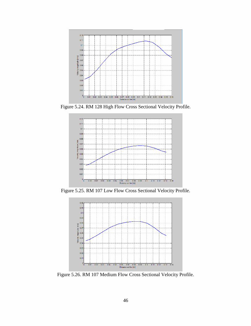
46
Figure 5.24. RM 128 High Flow Cross Sectional Velocity Profile.
Figure 5.25. RM 107 Low Flow Cross Sectional Velocity Profile.
Figure 5.26. RM 107 Medium Flow Cross Sectional Velocity Profile.

47
Figure 5.27. RM 107 High Flow Cross Sectional Velocity Profile.
Figure 5.28. RM 104 Low Flow Cross Sectional Velocity Profile.
Figure 5.29. RM 104 Medium Flow Cross Sectional Velocity Profile.

48
Figure 5.30. RM 104 High Flow Cross Sectional Velocity Profile.
Figure 5.31. RM 61 Low Flow Cross Sectional Velocity Profile.
Figure 5.32. RM 61 Medium Flow Cross Sectional Velocity Profile.

49
Figure 5.33. RM 61 High Flow Cross Sectional Velocity Profile.
Figure 5.34. RM 59 Low Flow Cross Sectional Velocity Profile.
Figure 5.35. RM 59 Medium Flow Cross Sectional Velocity Profile.

50
(Table Continued)
Figure 5.36. RM 59 High Flow Cross Sectional Velocity Profile.
5.5. Discussion
Analysis of the PIV results are positive. PIVlab data analysis matched the flow paths and
patterns well. Areas of flow in the channel where higher speeds are clearly visible in the videos
coincide with higher velocities that can be seen in the heat maps of the average cross-sectional
surface velocity frames. Furthermore, observed mean surface velocities matched theoretical
surface velocity values well. Most of the observations had a percent difference of less than 10
and most of the observations were lower than the theoretical values. There were only 5
observations where the observed values were greater than the theoretical. These instances
occurred at the higher flows of RM 61 and for all the flows at RM 59. This may be attributed to
the geometry of the locations, which are in a relatively straight portion of the river, but this
would need to be further investigated to be determined for certain. The average percent
difference by location for all flows can be seen in Table 5.2. RM 107 had the lowest difference
with 6.78%, and RM 128 had the highest with 16.04%. The average percent difference by
flowrate for all locations can be seen in Table 5.3. The high flows had the lowest difference with
-0.91%, and the medium flows had the highest with 7.78%. The average percent difference for
all observations was 10.52%. This information shows that analysis with PIVlab yields accurate
results. It should be noted that all velocity magnitudes are assumed to be the x-component of
velocity vectors (perpendicular to the cross-section) for calculated observed and theoretical
surface velocities. Direction of the vectors was not considered. This assumption does not
significantly affect calculated surface velocities.
Table 5.2. Average Percent Difference by Location.
Location Cross Section % Difference
Bonnet
Carre'
RM 130
(Bend) 11.73
RM 128
(Crossing) 16.04

51
Carrolton
RM 107
(Crossing) 6.78
RM 104
(Bend) 8.92
Alliance
RM 61
(Crossing) -9.25
RM 59
(Bend) -9.48
Table 5.4. Average Percent Difference by Flowrate.
Flowrate % Difference
Low 5.50
Medium 7.78
High -0.91
All Observations 10.52
Some interesting observations can be seen in the results. At RM 130 (Figures 5.1. – 5.3.)
higher velocities appeared closer to the inside of the bend which contradicts typical expectations
of flow around a bend. One may expect higher velocities on the outside curve, but this
observation can be attributed to the spatial context of the location. This location sits at the second
curve of two successive roughly 90º bends (Figure 4.2.). At RM 104 (Figures 5.10. – 5.12.)
narrow high speeds appear near the middle of the bend. Again, this contradicts typical
expectations of flow around a bend, but this can be attributed to the sharpness of curvature of the
location (Figure 4.3.). Typical expected velocity distributions of flow around a bend was
observed at RM 61 (Figures 5.16. – 5.18.). This location is a very gentle bend in a relatively
straight potion of the river model (Figure 4.4.).
It may be interpreted that the narrow shape of the cross-sectional velocity profiles could
be attributed to the scale effects discussed in this thesis. However, without further investigation,
that cannot be stated for certain. The literature states the scale effects may be observable in the
vertical velocity profile shape, but perhaps a similar observation may be made in the 2-
dimensional cross-sectional velocity profile shape as well.
Table 5.3. Average Percent Difference by Location.

52
Chapter 6. Conclusions
The results of the flow visualization studies presented in this thesis have effectively
addressed and answered the questions raised in the objective. Due to model distortion, the
Froude scaled physical model did not meet Reynolds number similitude. This leads to the
presence of scale effects impacting hydrodynamic patterns like turbulence and flow around
bends. For one, qualitative data extracted from the dye studies clearly show increasing levels of
mixing with increasing flowrates. While not definitive, the relatively high levels of mixing at
medium and high flowrates indicate that the flow is in the rough turbulent regime. Therefore,
more quantitative studies should be done to see if the levels of turbulence can be measured.
Secondly, three-dimensional hydrodynamics were also observed through dye injection. Helical
flow in the bends of the model river were observable, especially in sharper bends. The utilization
of PIV allowed two-dimensional surface velocities to be quantitatively measured. Observations
show good agreement when comparing results to theoretical values. Most observations were
within a 10% difference of theoretical values. Only two observations exceeded a 20% difference
(-21.65% and 22.30%). The average percent difference for all observations was 10.52%. The
results of the PIV analysis prove that the method is viable for measuring two-dimensional
surface velocities and that PIVlab is affective at calculating those results. Although the
hydrodynamic patterns were able to be quantified via PIV, the impact of model distortion on the
2-dimensional surface velocities could not be quantified. The results of this thesis potentially
offer observations of the scale effects associated with the distortion of a hydraulic physical
model. The narrowing of dye plumes and the cross sectional velocity profile shape measured via
PIV may be a visual representation of their existence. However, this cannot be stated for certain
without further investigation.
6.1. Limitations
The limitations of this study should be noted for the success of future flow visualization
studies on the LRMPM and other distorted models like it. For dye injection, lighting and camera
quality may limit the results. Proper lighting of the dye allows for clear visualization of flow and
enhanced image quality makes specific intricacies more observable. Fluctuating flow, cross
section digitalization, water level sensors, and bed measurements for determining cross sectional
area and wetted perimeter could affect the calculation of Reynolds number. Qualitatively, dye
definition may be affected by interference with suspended sediment, otherwise known as
mechanical dispersion. This may affect the appearance of mixing at higher flowrates. Dye
injection flow speed may also impact the observation. Although Mariotte bottles were used to
inject a constant flow rate, flow speed is controlled by the height of the vent tube, h, above the
water (Holden, 2005). The equation for the velocity of dye injection is given by,
𝑣𝑑𝑦𝑒 = √2𝑔ℎ
(6.1.)
Matching the flow speed in the channel would have required using a smaller bottle with a very
small distance of the vent tube above the surface of the water (fractions of an inch).
For PIV, lighting and camera quality may limit results, as well as camera angle and distance.
However, the studies were conducted in accordance to cited recommendations. Fluctuating flow,
cross sectional digitalization, water level sensors, and bed measurements may also affect the

53
calculation of theoretical surface velocities. Additionally, seeding concentration may affect the
analysis of observed surface velocities. Merzkirch (1987) recommends a medium to high
concentration. Although the low flows were seeded with fewer particles (300) than the medium
and high flows (600), the results show that low flows had the smallest percent difference
between observed and theoretical values. Lastly, particle collisions may impact observed results.
Fluctuating flow and higher speeds may force particles to interfere with each other, which may
introduce inaccurate velocity measurements. However, this was addressed by activating the
interpolation feature in PIVlab.
6.2. Recommendations
From this experience, some recommendations should be considered for future flow
visualization studies of this kind on the LMRPM or similar models. A more robust lighting
source would enhance the visual quality of dye injection studies. The UV flashlight was
sufficient for PIV, but with the lighting issues that were encountered during the dye injection
studies, a larger lighting source is recommended. Furthermore, a higher quality imaging camera
may offer a higher resolution observation for dye injection. It seemed that the raw videos lacked
the image quality to distinguish flow structures and features that were observable by the naked
eye and a higher quality camera may improve video observations. A unique idea would be to
inject hot water into the channel and record the observation with a thermal imaging camera. The
camera may be able to observe flow structure from the injected water and this would eliminate
any lighting concerns. Further development of a dye injection mechanism should also be
considered to match water velocity. A control pump could be used to regulate speed. Running
experiments without suspended sediment could be performed to investigate the impact of
mechanical dispersion. However, sediment transport would not be reliably simulated without the
injection of sediment into the model. Consistency of PIV seeding concentrations could be
investigated in order to determine optimization. It does seem that the method presented in this
thesis, using PIVlab, is sufficient. Furthermore, PIVlab can be used to produce vorticity,
divergence, and shear and strain rates which can be used to study hydrodynamics in the LMRPM
and other models like it. Perhaps, further PIV studies could be used to investigate these flow
parameters or upstream flow, which could be observed with PIVlab analysis. The impact of
model distortion on 2-dimensional hydrodynamics could potentially be investigated by observing
3-dimensional hydrodynamics and comparing the results since the literature states that scale
effects are mostly present in vertical velocity profiles. Interesting studies that could be applied to
the LMRPM include dye injection and PIV studies in sediment diversions and other features of
flow separation to study and/or characterize flow structure at defined geometries. Other potential
studies could be done in other locations with interesting bends and crossings. Lastly, dye
injection could also be used to mimic silts and clays since model sediment is designed to only
mimic river sand.

54
Appendix A. Turbulence Similitude in Geometrically Distorted Models
The following is the derivation for scale effects from nonsimilar turbulent Reynolds
stress terms provided by Hughes (1993). Strict similitude criteria for hydrodynamic modeling are
found by casting the Navier Stokes equations into nondimensional form and requiring that all
dimensionless coefficients remain the same in the model and prototype. The four governing
equations for incompressible surface flow are given by the continuity and Navier-Stokes
equations, i.e.,
continuity 𝜕𝑢
𝜕𝑥+
𝜕𝑣
𝜕𝑦+
𝜕𝑤
𝜕𝑧= 0
(A.1.)
x-direction momentum
𝜕𝑢
𝜕𝑡+ 𝑢
𝜕𝑢
𝜕𝑥+ 𝑣
𝜕𝑢
𝜕𝑦+ 𝑤
𝜕𝑢
𝜕𝑧
= −1
𝜌
𝜕𝑝
𝜕𝑥+ 𝜈 (
𝜕2𝑢
𝜕𝑥2+
𝜕2𝑢
𝜕𝑦2+
𝜕2𝑢
𝜕𝑧2) − [
𝜕
𝜕𝑥(𝑢′2 ) +
𝜕
𝜕𝑦(𝑢′𝑣′ ) +
𝜕
𝜕𝑧(𝑢′𝑤′ )]
(A.2.)
y-direction momentum
𝜕𝑣
𝜕𝑡+ 𝑢
𝜕𝑣
𝜕𝑥+ 𝑣
𝜕𝑣
𝜕𝑦+ 𝑤
𝜕𝑣
𝜕𝑧
= −1
𝜌
𝜕𝑝
𝜕𝑦+ 𝜈 (
𝜕2𝑣
𝜕𝑥2+
𝜕2𝑣
𝜕𝑦2+
𝜕2𝑣
𝜕𝑧2) − [
𝜕
𝜕𝑥(𝑢′𝑣′ ) +
𝜕
𝜕𝑦(𝑣′2 ) +
𝜕
𝜕𝑧(𝑣′𝑤′ )]
(A.3.)
z-direction momentum
𝜕𝑤
𝜕𝑡+ 𝑢
𝜕𝑤
𝜕𝑥+ 𝑣
𝜕𝑤
𝜕𝑦+ 𝑤
𝜕𝑤
𝜕𝑧
= −1
𝜌
𝜕𝑝
𝜕𝑧− 𝑔 + 𝜈 (
𝜕2𝑤
𝜕𝑥2+
𝜕2𝑤
𝜕𝑦2+
𝜕2𝑤
𝜕𝑧2) − [
𝜕
𝜕𝑥(𝑢′𝑤′ ) +
𝜕
𝜕𝑦(𝑣′𝑤′ ) +
𝜕
𝜕𝑧(𝑤′2 )]
(A.4.)
where
t = time
x, y = horizontal coordinates
z = vertical coordinate
u, v, w = non turbulent horizontal components of velocity in the x, y, and z directions,
respectively
u’, v’, w’, = turbulent fluctuating components of velocity in the x, y, and z directions, respectively

55
g = gravitational acceleration
p = fluid pressure
ρ = fluid density
ν = fluid kinematic viscosity
Appropriate scaling criteria are derived from the equations of motion by expressing the
equations in nondimensional form using the following definitions and substituting for the
independent and dependent variables:
=𝑢
𝑉; 𝑣 =
𝑣
𝑉; =
𝑤
𝑊
=𝑥
𝑋; =
𝑦
𝑋; =
𝑧
𝑍
=𝑡
𝑇; =
𝑝
𝑃
(A.5.)
where
V = characteristic nonturbulent horizontal velocity
W = characteristic nonturbulent vertical velocity
X = characteristic horizontal length
Z = characteristic vertical length
T = characteristic time
P = characteristic pressure
Different characteristic lengths and velocities were chosen for the horizontal and vertical
directions to accommodate geometrically distorted hydrodynamic models. For convenience, the
same characteristic velocities were used to nondimensionalize the turbulent Reynolds stresses.
Making these substitutions into Equations A.1. through A.5., multiplying the continuity
equation by X/V, the horizontal momentum equations by X/V2, and the vertical momentum
equation by Z/W2 yields the nondimensional equations of motion.
continuity (nondimensional)
𝜕
𝜕+
𝜕𝑣
𝜕+ (
𝑋𝑊
𝑍𝑉)
𝜕
𝜕= 0
(A.6.)
x-direction momentum (nondimensional)

56
(𝑋
𝑉𝑇)
𝜕
𝜕+
𝜕
𝜕+ 𝑣
𝜕
𝜕+ (
𝑋𝑊
𝑍𝑉)
𝜕
𝜕
= − (𝑃
𝜌𝑉2)
𝜕
𝜕+ [(
𝜈
𝑋𝑉)
𝜕2
𝜕2+ (
𝜈
𝑋𝑉)
𝜕2
𝜕2+ (
𝑣𝑋
𝑍2𝑉)
𝜕2
𝜕2]
− [𝜕
𝜕(′2 ) +
𝜕
𝜕(′𝑣′ ) + (
𝑋𝑊
𝑍𝑉)
𝜕
𝜕(′′ )]
(A.7.)
y-direction momentum (nondimensional)
(𝑋
𝑉𝑇)
𝜕𝑣
𝜕+
𝜕𝑣
𝜕+ 𝑣
𝜕𝑣
𝜕+ (
𝑋𝑊
𝑍𝑉)
𝜕𝑣
𝜕
= − (𝑃
𝜌𝑉2)
𝜕
𝜕+ [(
𝜈
𝑋𝑉)
𝜕2
𝜕2+ (
𝜈
𝑋𝑉)
𝜕2𝑣
𝜕2+ (
𝑣𝑋
𝑍2𝑉)
𝜕2
𝜕2]
− [𝜕
𝜕(′𝑣′ ) +
𝜕
𝜕(𝑣′2 ) + (
𝑋𝑊
𝑍𝑉)
𝜕
𝜕(𝑣′′ )]
(A.8.)
z-direction momentum (nondimensional)
(𝑍
𝑊𝑇)
𝜕
𝜕+ (
𝑍𝑉
𝑋𝑊) (
𝜕
𝜕+ 𝑣
𝜕
𝜕) +
𝜕
𝜕
= − (𝑃
𝜌𝑊2)
𝜕
𝜕− (
𝑔𝑍
𝑊2) + [(
𝜈𝑍
𝑋2𝑉)
𝜕2
𝜕2+ (
𝜈𝑍
𝑋2𝑊)
𝜕2
𝜕2+ (
𝑣
𝑍𝑊)
𝜕2
𝜕2]
− [(𝑍𝑉
𝑋𝑊) (
𝜕
𝜕(′′ ) +
𝜕
𝜕(𝑣′′ )) +
𝜕
𝜕(′2 )]
(A.9.)
If two systems are governed by the previous nondimensional equations, then the solution
in terms of the nondimensional parameters will be the same for each system provided all
dimensionless coefficients remain unchanged. This means complete similitude would be
achieved for any free surface hydrodynamic phenomena governed by the formulation of the
Navier-Stokes equations if the value of each dimensionless coefficient in Equations A.6. through
A.9. remains constant between prototype and model. Note that all nondimensional terms without
coefficients will be in similitude.
Focusing attention on the turbulence terms, the only dimensionless coefficients are
(XW/ZV) and its inverse. Therefore, the requirement for similitude of the differential turbulence
Reynolds stress terms having this coefficient is simply,
(𝑋𝑊
𝑍𝑉)
𝑝𝑟𝑜𝑡𝑜𝑡𝑦𝑝𝑒= (
𝑋𝑊
𝑍𝑉)
𝑚𝑜𝑑𝑒𝑙

57
(A.10.)
or rearranged…
(𝑋𝑝
𝑋𝑚) (
𝑊𝑝
𝑊𝑚) = (
𝑍𝑝
𝑍𝑚) (
𝑉𝑝
𝑉𝑚)
(A.11.)
The requirement given by Equation A.10. can be expressed in terms of scale ratios as:
𝑋𝑟
𝑍𝑟=
𝑉𝑟
𝑊𝑟
(A.12.)
where, by definition, a scale ratio is the ratio of a parameter in the prototype to the value of the
same parameter in the model.
Because the scaling ratio for horizontal and vertical velocity should be the same, the
scaling requirement of Equations A.4.-A.12. can only be fulfilled when Xr = Zr, which is the
requirement for a geometrically undistorted physical model. Therefore, turbulent Reynolds stress
terms containing this dimensionless coefficient will not be in similitude in a geometrically
distorted model, and this introduces a scale effect. From Equations A.4.-A.6. through A.4.-A.9.
the following can be concluded:
Turbulence terms in similitude
𝜕
𝜕𝑥(𝑢′2 );
𝜕
𝜕𝑦(𝑢′𝑣′ );
𝜕
𝜕𝑥(𝑢′𝑣′ );
𝜕
𝜕𝑦(𝑣′2 );
𝜕
𝜕𝑧(𝑤′2 )
(A.13.)
Turbulence terms not in similitude
𝜕
𝜕𝑥(𝑢′𝑣′ );
𝜕
𝜕𝑦(𝑣′𝑤′ );
𝜕
𝜕𝑧(𝑢′𝑤′ );
𝜕
𝜕𝑧(𝑣′𝑤′ )
(A.14.)
The four turbulence terms, in Equation A.13., involving squares or cross products of the
horizontal turbulent velocity fluctuations and the term containing the square of the vertical
turbulent velocity fluctuation are in similitude in distorted models, whereas the four Reynolds
stress terms containing the cross-product of horizontal and vertical velocities, in Equation A.14.,
do not fulfill the requirement and represent the potential scale effect.
The two nonsimilar turbulent Reynolds stress terms contained in the horizontal
momentum equations are larger in the model than they should be by a factor equal to the
geometric distortion, Ω, i.e.,
𝛺 [𝜕
𝜕(′′ );
𝜕
𝜕(𝑣′′ )]
𝑝𝑟𝑜𝑡𝑜𝑡𝑦𝑝𝑒= [
𝜕
𝜕(′′ );
𝜕
𝜕(𝑣′′ )]
𝑚𝑜𝑑𝑒𝑙
(A.15.)

58
This implies that the vertical variation of the turbulent velocity products u’w’ and v’w’ is greater
in the distorted model than in the prototype.
Conversely, the two nonsimilar turbulent Reynolds stress terms contained in the vertical
momentum equation are smaller in the model than they should be by a factor equal to the inverse
of the geometric distortion, 1/Ω, i.e.,
1
𝛺[
𝜕
𝜕(′′ );
𝜕
𝜕(𝑣′′ )]
𝑝𝑟𝑜𝑡𝑜𝑡𝑦𝑝𝑒
= [𝜕
𝜕(′′ );
𝜕
𝜕(𝑣′′ )]
𝑚𝑜𝑑𝑒𝑙
(A.16.)
In this case the horizontal variation of the turbulent velocity products u’w’ and v’w’ is less in the
distorted model than in the prototype.

59
Appendix B. Flow Similitude in Bends of Geometrically Distorted Models
Hughes & Pizzo (2003) state that similitude requirements for flow around bends are the
same as before, except now the governing equations are presented in cylindrical coordinates.
Here, turbulence terms and viscous shear terms have been omitted from the momentum
equations to focus on the scale effects associated with flow acceleration around river bends in
physical models.
continuity 𝜕𝑣𝑟
𝜕𝑟+
𝑣𝑟
𝑟+
1
𝑟
𝜕𝑣𝜃
𝜕𝜃+
𝜕𝑣𝑧
𝜕𝑧= 0
(B.1.)
r-direction momentum
𝜕𝑣𝑟
𝜕𝑡+ 𝑣𝑟
𝜕𝑣𝑟
𝜕𝑟+
𝑣𝜃
𝑟
𝜕𝑣𝑟
𝜕𝜃−
𝑣𝜃2
𝑟+ 𝑣𝑧
𝜕𝑣𝑟
𝜕𝑧= −
1
𝜌
𝜕𝑝
𝜕𝑟
(B.2.)
-direction momentum
𝜕𝑣𝜃
𝜕𝑡+ 𝑣𝑟
𝜕𝑣𝜃
𝜕𝑟+
𝑣𝜃
𝑟
𝜕𝑣𝜃
𝜕𝜃+
𝑣𝑟𝑣𝜃
𝑟+ 𝑣𝑧
𝜕𝑣𝜃
𝜕𝑧= −
1
𝜌𝑟
𝜕𝑝
𝜕𝜃
(B.3.)
z-direction momentum
𝜕𝑣𝑧
𝜕𝑡+ 𝑣𝑟
𝜕𝑣𝑧
𝜕𝑟+
𝑣𝜃
𝑟
𝜕𝑣𝑧
𝜕𝜃+ 𝑣𝑧
𝜕𝑣𝑧
𝜕𝑧= −
1
𝜌
𝜕𝑝
𝜕𝑧+ 𝑔
(B.4.)
where
t = time
r = horizontal cross-channel (radial) coordinate
= horizontal along-channel (angular) coordinate
z = vertical coordinate
vr = non turbulent horizontal cross-channel component of velocity in the r direction
v = non turbulent along-channel component of velocity in the direction
vz = non turbulent vertical component of velocity in the z direction
g = gravitational acceleration
p = fluid pressure
ρ = fluid density

60
Appropriate scaling criteria are derived from the equations of motion by expressing the
equations in nondimensional forms using the following definitions and substituting for the
independent and dependent variables:
𝑣 =𝑣𝑟
𝑉; 𝑣 =
𝑣𝜃
𝑉; 𝑣 =
𝑣𝑧
𝑉; =
𝑡
𝑇
=𝑟
𝑋; =
𝑧
𝑍; =
𝑝
𝑃
(B.5.)
where
V = characteristic nonturbulent horizontal velocity
X = characteristic horizontal length
Z = characteristic vertical length
T = characteristic time
P = characteristic pressure
Different characteristic lengths were chosen for the horizontal and vertical directions to
accommodate geometrically distorted hydrodynamic models. For convenience, the same
characteristic velocities were used to nondimensionalize the radial, tangential, and vertical
velocity components.
Making these substitutions into Equations B.1. through B.4., multiplying the continuity
equation by X/V, the horizontal momentum equations by X/V2, and the vertical momentum
equation by Z/V2 yields the nondimensional equations of motion in cylindrical coordinates.
continuity (nondimensional) 𝜕𝑣
𝜕+
𝑣
+
1
𝜕𝑣
𝜕𝜃+ (
𝑋
𝑍)
𝜕𝑣
𝜕= 0
(B.6.)
r-direction momentum (nondimensional)
(𝑋
𝑉𝑇)
𝜕𝑣
𝜕+ 𝑣
𝜕𝑣
𝜕+
𝑣
𝜕𝑣
𝜕𝜃−
𝑣2
+ (
𝑋
𝑍) 𝑣𝑧
𝜕𝑣
𝜕= − (
𝑃
𝜌𝑉2)
𝜕
𝜕
(B.7.)
-direction momentum (nondimensional)
(𝑋
𝑉𝑇)
𝜕𝑣
𝜕+ 𝑣
𝜕𝑣
𝜕+
𝑣
𝜕𝑣
𝜕𝜃+
𝑣𝑣
+ (
𝑋
𝑍) 𝑣𝑧
𝜕𝑣
𝜕= − (
𝑃
𝜌𝑉2)
1
𝜕
𝜕𝜃
(B.8.)
z-direction momentum (nondimensional)
(𝑍
𝑉𝑇)
𝜕𝑣
𝜕+ (
𝑍
𝑋) 𝑣
𝜕𝑣
𝜕+ (
𝑍
𝑋)
𝑣
𝜕𝑣
𝜕𝜃+ 𝑣
𝜕𝑣
𝜕= − (
𝑃
𝜌𝑉2)
𝜕
𝜕+ (
𝑔𝑍
𝑉2)

61
(B.9.)
Just as before, if two systems are governed by the previous nondimensional equations,
then the solution in terms of the nondimensional parameters will be the same for each system
provided all dimensionless coefficients remain unchanged. This means complete similitude
would be achieved for any free surface hydrodynamic phenomena governed by the cylindrical
form of the Navier-Stokes equations if the value of each dimensionless coefficient in Equations
B.6. through B.9. remains constant between prototype and model. Note that all nondimensional
terms without coefficients will be in similitude.
For steady flow, the only potential scale effects arise from the convective accelerations,
and the only dimensionless coefficients are (X/Z) and its inverse. Therefore, the requirement for
similitude of the convective acceleration is simply:
(𝑋
𝑍)
𝑝𝑟𝑜𝑡𝑜𝑡𝑦𝑝𝑒= (
𝑋
𝑍)
𝑚𝑜𝑑𝑒𝑙
(B.10.)
or expressed in terms of scale ratios
𝑋𝑟 = 𝑍𝑟
(B.11.)
which means a geometrically undistorted model. From Equations B.6. through B.9. the following
can be concluded:
convective acceleration terms in similitude
𝑣𝑟
𝜕𝑣𝑟
𝑟;
𝑣𝜃
𝑟
𝜕𝑣𝑟
𝜕𝜃;
𝑣𝜃2
𝑟; 𝑣𝑟
𝜕𝑣𝜃
𝜕𝑟;
𝑣𝜃
𝑟
𝜕𝑣𝜃
𝜕𝜃;𝑣𝑟𝑣𝜃
𝑟; 𝑣𝑧
𝜕𝑣𝑧
𝜕𝑧
(B.12.)
convective acceleration terms not in similitude
𝑣𝑧
𝜕𝑣𝑟
𝜕𝑧; 𝑣𝑧
𝜕𝑣𝜃
𝜕𝑧; 𝑣𝑟
𝜕𝑣𝑧
𝜕𝑟;
𝑣𝜃
𝑟
𝜕𝑣𝑧
𝜕𝜃
(B.13.)
The two nonsimilar convective accelerations contained in the horizontal direction
momentum equations are larger in the model than they should be by a factor equal to the
geometric distortion, i.e.,
Ω (𝑣𝑧
𝜕𝑣
𝜕; 𝑣
𝜕𝑣
𝜕)
𝑝𝑟𝑜𝑡𝑜𝑡𝑦𝑝𝑒= (𝑣𝑧
𝜕𝑣
𝜕; 𝑣
𝜕𝑣
𝜕)
𝑚𝑜𝑑𝑒𝑙
(B.14.)
This implies that horizontal convective accelerations due to vertical gradients of the radial and
tangential velocities (vr, v) are greater in the distorted model than in the prototype.

62
Conversely, the two nonsimilar convective accelerations contained in the vertical
momentum equation are smaller in the model than they should be by a factor equal to the inverse
of the geometric distortion, i.e.,
1
Ω(𝑣𝑟
𝜕𝑣
𝜕;
𝑣
𝜕𝑣
𝜕𝜃)
𝑝𝑟𝑜𝑡𝑜𝑡𝑦𝑝𝑒
= (𝑣𝑟
𝜕𝑣
𝜕;
𝑣
𝜕𝑣
𝜕𝜃)
𝑚𝑜𝑑𝑒𝑙
(B.15.)
In this case the vertical convective accelerations due to horizontal gradients of the vertical
velocity (vz) are less in the distorted model than in the prototype.

63
Appendix C. Experimental Setup Images
All images are facing downstream.
Figure C.1. Experimental Setup at RM 130.
Figure C.2. Experimental Setup at RM 128.

64
Figure C.3. Experimental Setup at RM 107.
Figure C.4. Experimental Setup at RM 104.
Figure C.5. Experimental Setup at RM 61

65
Figure C.6. Experimental Setup at RM 59.

66
Appendix D. Materials Images
Figure D.1. All Materials Used
Figure D.2. Nikon Coolpix B500 Digital Camera.

67
Figure D.3. McDoer 100 LED UV Flashlight.
Figure D.4. 1.5 ft. (left) and 1.0 ft. (right) Tripods.
Figure D.5. Ruler and Caliper.

68
Figure D.6. UV Reactive Water Dye and Syringe.
Figure D.7. Mariotte Bottles.
Figure D.8. Green Water Based Acrylic Glow in the Dark Paint.

69
Figure D.9. HDPE Painted PIV Particles.
Figure D.10. Corona Stainless Steel Scoop Hand Shovel.
Figure D.11. Nylon Aquarium Fishing Nets.

70
References
BCG Engineering & Consultants Inc. (2015). Proof of concept report on tests of instrumentation,
automation, and hydraulics in a distorted scale physical model of a reach of the
mississippi river. (Tech. Report). State of Louisiana Coastal Protection and Restoration
Authority.
Blum, M., & Roberts, H. (2009). Drowing of the Mississippi Delta due to insufficient sediment
supply and global sea-level rise. Nature Geoscience, 2(7), 488-491.
Blum, M., & Roberts, H. (2012). The Mississippi Delta region: past, present, and future. Annual
Review of Earth and Planetary Sciences, 40(1), 655-683.
Chanson, H. (2004). Hydraulics of open channel flow. Elsevier Butterworth-Heinemann.
Chow, V. (1959). Open-channel hydraulics. McGraw-Hill Book Company, Inc.
CPRA, Coastal Protection and Restoration Authority (2012). Louisiana's Comprehensive Master
Plan for a Sustainable Coast. State of Louisiana Coastal Protection and Restoration
Authority.
CPRA, Coastal Protection and Restoration Authority (2017). Louisiana's Comprehensive Master
Plan for a Sustainable Coast. State of Louisiana Coastal Protection and Restoration
Authority.
Einstein, H., & Chien, N. (1956). Similarity of distorted river models with movable beds.
Transactions of the American Society of Civil Engineers, 121(1), 440-457.
Ettema, R., Arndt, R., Roberts, P., & Wahl, T. (2000). Hydraulic modeling: concepts and
practice. In E. a. Task Committee on Hydraulic Modeling, ASCE Manuals and Reports
on Engineering Practice (Vol. 97, pp. 361-397). American Society of Civil Engineers.
Franco, J. (1978). Guidelines for the design, adjustment, and operation of models for the study of
river sedimentation problems. (Tech. Report). DTIC Document.
Frostick, L., McLelland, S., & Mercer, T. (2011). Users guide to physical modelling and
experimentation: experience of the hydralab network. CRC Press.
Graveleau, F., Hurtrez, J., Dominguez, S., & Malavieille, J. (2011). A new experimental material
for modeling relief dynamics and interactions between tectonics and surface processes.
Tectonophysics, 513(1), 68-87.
Green, D. (2014). Modelling geomorphic systems: scaled physical models. Geomorphological
Techniques.
Holden, J. (2005). Mariotte Bottle - Use in Hydrology. In Water Encyclopedia: Ocenogrophy;
Meteorology; Physics and Chemistry; Water Law; and Water History, Art, and Culture
(pp. 503-504). John Wiley & Sons, Inc.
Hooper, M. (2019). Qualitative evaluation of a lightweight sediment for a physical model of the
Lower Mississippi River. PhD. Dissertation. Louisiana State University. Baton Rouge,
Louisiana.

71
Huang, H., Dabiri, D., & Gharib, M. (1997). On errors of digital particle velocimetry.
Measurement of Science and Technology, 8, 1427-1440.
Hughes, S. (1993). Physical models and laboratory techniques in coastal engineering. Advanced
Series on Ocean Engineering, 7.
Hughes, S., & Pizzo, G. (2003). Flow Table Study of Cook Inlet, Alaska. (Tech. Report). U.S.
Army Corps of Engineers.
Julien, P. (2002). River Mechanics. Cambridge University Press.
Kim, Y. (2006) Uncertainty analysis for non-intrusive measurement of river discharge using
image velocimetry. PhD. Thesis Dissertation. University of Iowa. Iowa City, Iowa.
Keane, R., & Adrian, R. (1993). Theory and simlation of particle image velocimetry.
Proceedings of SPIE - The International Society for Optical Engineering. 2052, pp. 477-
492. Bellingham, WA, United States: Society of Photo-Optical Instrumentation
Engineers.
Lin, C., Miau, J. C., Chou, J., Pan, D., & Lin, S. (1993). Flow visualization in a circular - to
rectangular transition duct. International Journal of Turbo and Jet-Engines, 10, 61-74.
LSU Center for River Studies. (2019, April 2). Retrieved from Coastal Protection and Restoration
Authority: http://coastal.la.gov/center-for-river-studies/
Marjang, N., (2008). Calculated surface velocity coefficients for prismatic open channels by
three-dimensional hydraulic modeling. PhD Dissertation. Utah State University. Logan,
Utah.
Maynord, S. (2006). Evaluation of the micromodel: An extremely small-scale movable bed
model. Journal of Hydraulic Engineering, 132(4), 343-353.
Merzkirch, W. (1987). Flow Visualization. Academic Press, Inc.
Miau, Jiun-Jih, Leu, T., Chou, J., Lin, S., & Lin, C. (1990). Flow distortion in a circular-to-
rectangular transition duct. AIAA Journal, 28, 1447-1456.
Muste, M., Xiong, Z., Schöne, J., & Li, Z. (2004). Validation and extension of image
velocimetry capabilities for flow diagnostics in hydraulic modeling. Journal of Hydraulic
Engineering, 130(3), 175-185.
Parger, G. (1978). Self-formed straight rivers with equilibrium banks and mobile bed. Part 1. The
sand-silt river. Journal of Fluid Mechanics, 89(1), 109-125.
Prashun, A. (1987). Fundamentals of Hydraulic Engineering. Pearson.
Raffel, M., Willert, C., Wereley, S., & Kompenhans, J. (2007). Particle Image Velocimetry - A
Practical Guide, Second Edition. New York, NY: Springer.
Shen, H. (2012). Movable Bed Physical Models (Vol. 312). Springer Science and Buisness
Media.

72
SOGREAH Consultants. (2004). Small scale physical model of the Mississippi River Delta.
(Tech. Report). State of Louisiana - Department of Natural Resources.
Stanley, D., & Warne, A. (1994). Worldwide initiation of Holocene marine deltas by
deglaciation of sea-level rise. Science, 265, 228-231.
Sutarto, T. (2015). Application of large scale particle image velocimetry (LSPIV) to identify
flow pattern in a channel. Procedia Engineering, 125, 213-219.
Thielicke, W., & Stamhius, E. (2014). PIVlab - Towards a user friendly, affordable and accurate
digital particle image velocimetry in MATLAB. Journal of Open Research Software,
2(30).
Thielicke, W. (2014). The Flapping Flight of Birds - Analysis and Application. PhD Thesis.
University of Groningen. Groningen, Netherlands.
Tsujimoto, T. (1978). Probabilistic model of the process of bed load transport and its application
to mobile bed problems. PhD Thesis. Kyoto University. Kyoto, Japan
USACE, US Army Corps of Engineers (2019, April 2). The Mississippi River Drainage Basin.
Retrieved from US Army Corps of Engineers New Orleans District:
https://www.mvn.usace.army.mil/Missions/Mississippi-River-Flood-Control/Mississippi-
River-Tributaries/Mississippi-Drainage-Basin/
Warnock, J. (1950). Hydraulic similitude. Engineering Hydraulics, 136-176.
Yalin, M. (1971). Theory of Hydraulic Models. Macmillan.

73
Vita
Patrick Lyall Scott was born in Lafayette, Louisiana in October 1993. He attended
Cathedral Carmel School and Saint Thomas More Catholic High School in Lafayette, Louisiana.
In December of 2016 he received his Bachelor’s degree in Civil and Environmental Engineering
from Louisiana State University. He was awarded a graduate assistantship with the Center for
GeoInformatics at LSU to conduct geodetic research on subsidence along the northern Gulf of
Mexico under the guidance of the late Dr. Joshua Kent in January 2017. He later received
another graduate assistantship with the LSU Center for River Studies to conduct research on
sediment transport in the Lower Mississippi River Physical Model under the guidance of Dr.
Clinton Willson in January 2018.