One-Way Analysis of Variance (One-Way ANOVA)

The objectives of this lesson are to learn:

• the definition/purpose of One-Way Analysis of Variance

• the use of One-Way ANOVA

• the use of SPSS to complete a One-Way Analysis of Variance

• the interpretations of results

Definition

One-Way ANOVA involves examination of the significant differences between means of

three or more groups on one factor or dimension. For example, you might want to know

whether five groups of people (below 20, 21-30, 31-40, 41-50, above 50) differ in their

living expenses (per month).

When to Use One-Way ANOVA Any analysis where:

• There is only one dimension or factor (dependent variable)

• There are three or more groups of the factor (independent variable)

• One is interested in looking at mean differences across these groups

Assumptions:

• Steps for a One-Way ANOVA Using SPSS We will use a step-by-step approach to go through the steps for a one-way ANOVA using

SPSS statistical analysis package. Here is the background information of the sample data

we are using here.

Number of subjects: 60

Independent variable (Factor): Primary disability types including Physical (code = 1),

mental (code = 2), and intellectual (code = 3) disabilities.

Dependent variable: Vocational rehabilitation service cost (VRS cost)

Data: Table 1

Table 1

Steps for One-Way ANOVA: Step 1 : A statement of statistical hypothesis

0 1 2 3:H µ µ µ= = or means for all groups are equal OR all jµ s are equal

There is no significant difference in vocational rehabilitation service cost

between disability types

:aH at least one mean differs from the rest.

Physical D isability M ental disability Intellectual D isability

385 900 325355 900 300340 965 305400 965 365685 925 125655 915 140650 975 155625 985 335585 1050 115595 980 135580 975 105580 825 99625 735 135655 625 245700 975 305425 875 225355 925 235755 1050 222655 950 280538 875 246

Step 2 : Setting the α level of risk associated with the null hypothesis (or Type I error)

The level of Type I error is .05.

Step 3: Assumptions testing

Assumption 1: Normally distributed data: It is assumed that the data are from a

normally distributed population. The rationale behind hypothesis

testing relies on having normally distributed populations and so if

this assumption is not met then the logic behind hypothesis testing

is flawed. Most researchers eyeball their sample data by using a

histogram on SPSS.

Analyze ⇒ Descriptive Statistics ⇒ Frequencies (Figure 1) Figure 1

Interpretation:

The curve demonstrates a bell-shape curve. The data appear to be

normally distributed.

Assumption 2: Homogeneity of variance: This assumption means that the

variances should not change systematically throughout the data. In

designs in which you examine several groups of subjects this

** Ignore the frequency table**

assumption means that each of these groups should have the same

variance. In other words, the variances of scores in different

populations are equal. This means that the unsystematic variation

in a population is the same for each treatment condition.

Analyze ⇒ Compare Means ⇒ One-Way ANOVA (Figure 2) Figure 2

Interpretation:

• One-way ANOVA assumes that the variances of the groups are all

equal.

• This table displays the result of the Levene test for homogeneity of

variances.

• The significance value .080 exceeds .05, suggesting that the variances

for the three groups of subjects are equal; therefore, the assumption is

justified.

Assumption 3: Independence: This assumption is the data from different subjects

are independent, which means that the behavior of one subject

does not influence the behavior of another.

Yes, the data that we use here are from different/independent subjects.

Step 4 & 5: Test statistic using SPSS/ interpreting results

After the assumptions are tested and justified, we now can begin to test the

statistic.

Analyze ⇒ Compare Means ⇒ One-Way ANOVA (Figure 3) Figure 3

Test of Homogeneity of Variances

VR Cost

2.636 2 57 .080

LeveneStatistic df1 df2 Sig.

Levene Test is the test used to examine the homogeneity of variances

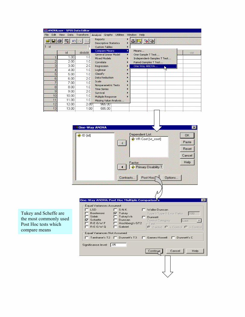
Tukey and Scheffe are the most commonly used Post Hoc tests which compare means

Descriptives

VR Cost

20 557.1500 131.13804 29.32336 495.7755 618.5245 340.00 755.0020 918.5000 100.21162 22.40800 871.5995 965.4005 625.00 1050.0020 219.8500 87.13889 19.48485 179.0677 260.6323 99.00 365.0060 565.1667 306.56291 39.57710 485.9731 644.3603 99.00 1050.00

Physical DisabilityMental DisabilityIntellectual DisabilityTotal

N Mean Std. Deviation Std. Error Lower Bound Upper Bound

95% Confidence Interval forMean

Minimum Maximum

SPSS Output and Interpretation

Oneway Interpretation: This table displays descriptive statistics for each group and for the entire data set.

N indicates the size of each group. The effects of unequal variances will be

reduced if the group sizes are approximately equal.

Mean shows the average values. One-Way ANOVA compares these sample

estimates to determine if the population means differ.

The standard deviation indicates the amount of variability of the scores in each

group. These values should be similar to each other for ANOVA to be

appropriate. Equality can be inspected via the Levene test [refer to Step 2 testing

assumption (2)].

The 95% confidence interval for the mean indicates the upper and lower bounds

which contain the true value of the population mean 95% of the time. None of the

disability group overlap with either of the other two groups.

Maximun and minimum values indicate the highest and lowest VRS costs for

each type of disabilities.

ANOVA

VR Cost

4883046 2 2441523.117 210.278 .000661822.1 57 11610.9145544868 59

Between GroupsWithin GroupsTotal

Sum ofSquares df Mean Square F Sig.

Interpretation:

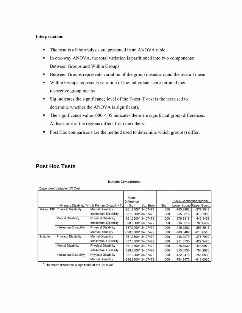
The results of the analysis are presented in an ANOVA table.

In one-way ANOVA, the total variation is partitioned into two components:

Between Groups and Within Groups.

Between Groups represents variation of the group means around the overall mean.

Within Groups represents variation of the individual scores around their

respective group means.

Sig indicates the significance level of the F-test (F-test is the test used to

determine whether the ANOVA is significant).

The significance value .000 <.05 indicates there are significant group differences.

At least one of the regions differs from the others.

Post Hoc comparisons are the method used to determine which group(s) differ. Post Hoc Tests

Multiple Comparisons

Dependent Variable: VR Cost

-361.3500* 34.07479 .000 -443.3482 -279.3518337.3000* 34.07479 .000 255.3018 419.2982361.3500* 34.07479 .000 279.3518 443.3482698.6500* 34.07479 .000 616.6518 780.6482

-337.3000* 34.07479 .000 -419.2982 -255.3018-698.6500* 34.07479 .000 -780.6482 -616.6518-361.3500* 34.07479 .000 -446.9970 -275.7030337.3000* 34.07479 .000 251.6530 422.9470361.3500* 34.07479 .000 275.7030 446.9970698.6500* 34.07479 .000 613.0030 784.2970

-337.3000* 34.07479 .000 -422.9470 -251.6530-698.6500* 34.07479 .000 -784.2970 -613.0030

(J) Primary Disability TypMental DisabilityIntellectual DisabilityPhysical DisabilityIntellectual DisabilityPhysical DisabilityMental DisabilityMental DisabilityIntellectual DisabilityPhysical DisabilityIntellectual DisabilityPhysical DisabilityMental Disability

(I) Primary Disability TypPhysical Disability

Mental Disability

Intellectual Disability

Physical Disability

Mental Disability

Intellectual Disability

Tukey HSD

Scheffe

MeanDifference

(I-J) Std. Error Sig. Lower Bound Upper Bound95% Confidence Interval

The mean difference is significant at the .05 level.*.

Interpretation: This table lists the pairwise comparisons of the group means for all selected post

hoc procedures.

Mean difference lists the differences between the sample means.

Sig lists the probability that the population mean difference is zero (<.05).

A 95% confidence interval is constructed for each difference. If this interval

contains zero, the two groups do not differ.

In our example, using the Tukey HSD and Scheffe procedures, All the six pairs;

Physical Disability-Mental Disability, Physical Disability-Intellectual Disability,

Mental Disability-Physical Disability, Mental Diability-Intellectual Disability,

Intellectual Disability-Physical Disability, Intellectual Disability-Mental

Disability; confidence intervals do not contain zero. These groups differ in VRS

costs. Homogeneous Subsets

Interpretation: For the selected post hoc procedures, homogeneous groups are defined.

Each homogeneous group corresponds to a column of the table.

In our example, both Tukey and Scheffe tests determine the three

homogeneous groups are defined.

VR Cost

20 219.850020 557.150020 918.5000

1.000 1.000 1.00020 219.850020 557.150020 918.5000

1.000 1.000 1.000

Primary Disability TypeIntellectual DisabilityPhysical DisabilityMental DisabilitySig.Intellectual DisabilityPhysical DisabilityMental DisabilitySig.

Tukey HSD a

Scheffe a

N 1 2 3Subset for alpha = .05

Means for groups in homogeneous subsets are displayed.Uses Harmonic Mean Sample Size = 20.000.a.

The means for each level of the independent variable are listed in their

corresponding homogeneous group.

The three group differs from the each other.

Step 6: Conclusion Based on the results of One-Way ANOVA (p = .000 < .05), we rejected the null

hypothesis. At least one mean differed than the rest. The VRS cost of at least one type of

disability differed than the rest.

The Tukey HSD and Scheffe Post Poc Tests both indicated that all the three

groups differed than each other. The VRS cost for individuals with mental disabilities (M

= 918.5) were significant higher than the VRS cost for individuals with physical

disabilities (M = 557.15) and those with intellectual disabilities ((M = 219.85).

Individuals with physical disabilities had significant higher VRS cost than those with

intellectual disabilities.