Embed Size (px)
Citation preview
3/18/2013
1
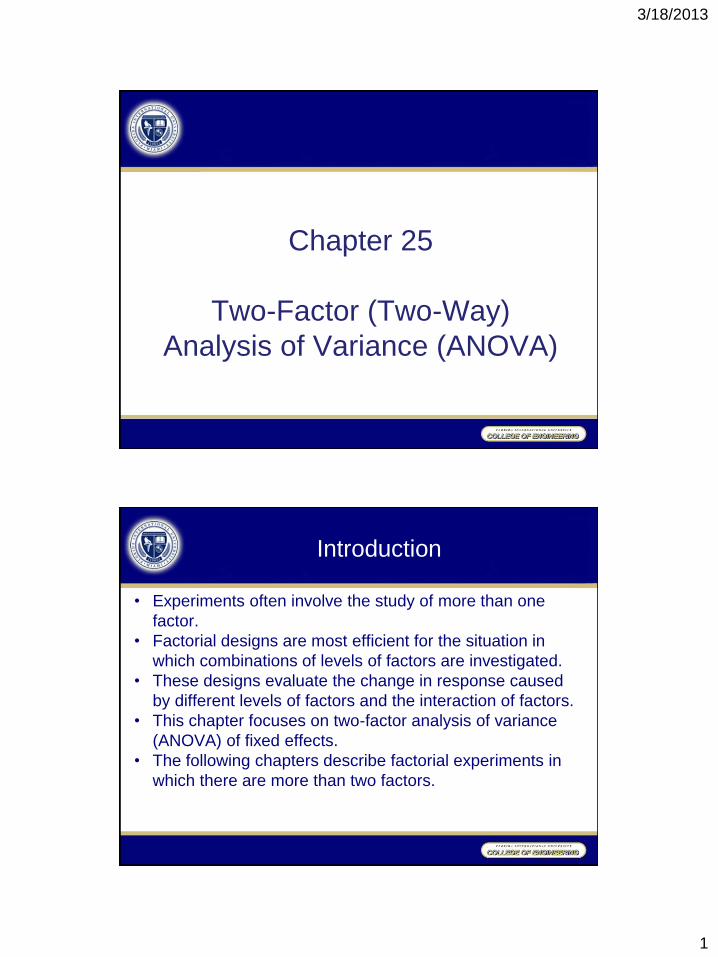
Chapter 25
Two-Factor (Two-Way)
Analysis of Variance (ANOVA)
Introduction
• Experiments often involve the study of more than one
factor.
• Factorial designs are most efficient for the situation in
which combinations of levels of factors are investigated.
• These designs evaluate the change in response caused
by different levels of factors and the interaction of factors.
• This chapter focuses on two-factor analysis of variance
(ANOVA) of fixed effects.
• The following chapters describe factorial experiments in
which there are more than two factors.
3/18/2013
2
25.1 Two-factor Factorial Design
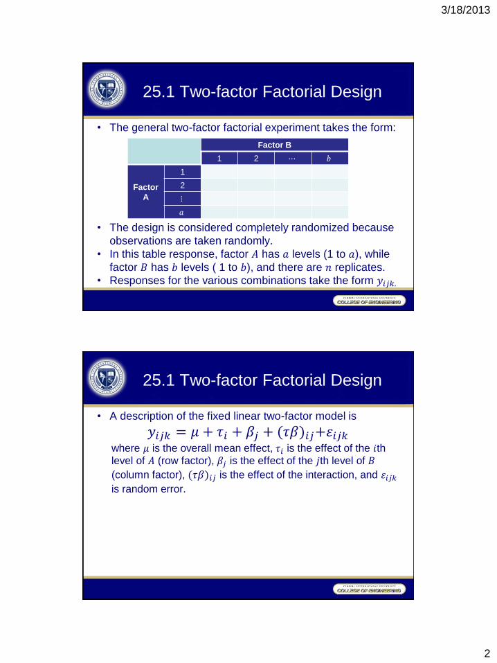
• The general two-factor factorial experiment takes the form:
Factor B
1 2 ⋯ 𝑏
Factor
A
1
2
⋮
𝑎
• The design is considered completely randomized because
observations are taken randomly.
• In this table response, factor 𝐴 has 𝑎 levels (1 to 𝑎), while
factor 𝐵 has 𝑏 levels ( 1 to 𝑏), and there are 𝑛 replicates.
• Responses for the various combinations take the form 𝑦𝑖𝑗𝑘.
25.1 Two-factor Factorial Design
• A description of the fixed linear two-factor model is
𝑦𝑖𝑗𝑘 = 𝜇 + 𝜏𝑖 + 𝛽𝑗 + (𝜏𝛽)𝑖𝑗+𝜀𝑖𝑗𝑘 where 𝜇 is the overall mean effect, 𝜏𝑖 is the effect of the 𝑖th
level of 𝐴 (row factor), 𝛽𝑗 is the effect of the 𝑗th level of 𝐵
(column factor), (𝜏𝛽)𝑖𝑗 is the effect of the interaction, and 𝜀𝑖𝑗𝑘
is random error.
3/18/2013
3
25.1 Two-factor Factorial Design
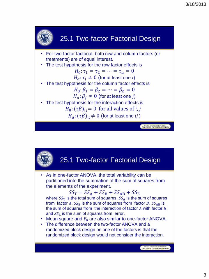
• For two-factor factorial, both row and column factors (or
treatments) are of equal interest.
• The test hypothesis for the row factor effects is
𝐻0: 𝜏1 = 𝜏2 = ⋯ = 𝜏𝑎 = 0
𝐻𝑎: 𝜏𝑖 ≠ 0 (for at least one 𝑖) • The test hypothesis for the column factor effects is
𝐻0: 𝛽1 = 𝛽2 = ⋯ = 𝛽𝑏 = 0
𝐻𝑎: 𝛽𝑗 ≠ 0 (for at least one 𝑗)
• The test hypothesis for the interaction effects is
𝐻0: (𝜏𝛽)𝑖𝑗= 0 for all values of 𝑖, 𝑗
𝐻𝑎: (𝜏𝛽)𝑖𝑗≠ 0 (for at least one 𝑖𝑗 )
25.1 Two-factor Factorial Design
• As in one-factor ANOVA, the total variability can be
partitioned into the summation of the sum of squares from
the elements of the experiment.
𝑆𝑆T = 𝑆𝑆A + 𝑆𝑆B + 𝑆𝑆AB + 𝑆𝑆E where 𝑆𝑆T is the total sum of squares, 𝑆𝑆A is the sum of squares
from factor 𝐴, 𝑆𝑆B is the sum of squares from factor 𝐵, 𝑆𝑆AB is
the sum of squares from the interaction of factor 𝐴 with factor 𝐵,
and 𝑆𝑆E is the sum of squares from error.
• Mean square and 𝐹0 are also similar to one-factor ANOVA. • The difference between the two-factor ANOVA and a
randomized block design on one of the factors is that the
randomized block design would not consider the interaction.
3/18/2013
4
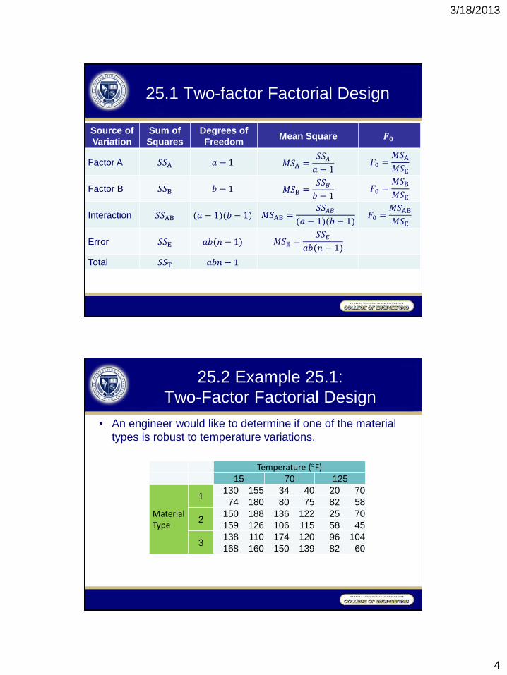
Source of
Variation
Sum of
Squares
Degrees of
Freedom Mean Square 𝑭𝟎
Factor A 𝑆𝑆A 𝑎 − 1 𝑀𝑆A =𝑆𝑆𝐴
𝑎 − 1 𝐹0 =
𝑀𝑆A
𝑀𝑆E
Factor B 𝑆𝑆B 𝑏 − 1 𝑀𝑆B =𝑆𝑆𝐵
𝑏 − 1 𝐹0 =
𝑀𝑆B
𝑀𝑆E
Interaction 𝑆𝑆AB (𝑎 − 1)(𝑏 − 1) 𝑀𝑆AB =𝑆𝑆𝐴𝐵
(𝑎 − 1)(𝑏 − 1) 𝐹0 =
𝑀𝑆AB
𝑀𝑆E
Error 𝑆𝑆E 𝑎𝑏(𝑛 − 1) 𝑀𝑆E =𝑆𝑆𝐸
𝑎𝑏(𝑛 − 1)
Total 𝑆𝑆T 𝑎𝑏𝑛 − 1
25.1 Two-factor Factorial Design
25.2 Example 25.1:
Two-Factor Factorial Design
• An engineer would like to determine if one of the material
types is robust to temperature variations.
Temperature (F)
15 70 125
Material Type
1 130 155 34 40 20 70
74 180 80 75 82 58
2 150 188 136 122 25 70
159 126 106 115 58 45
3 138 110 174 120 96 104
168 160 150 139 82 60
3/18/2013
5
25.2 Example 25.1:
Two-Factor Factorial Design
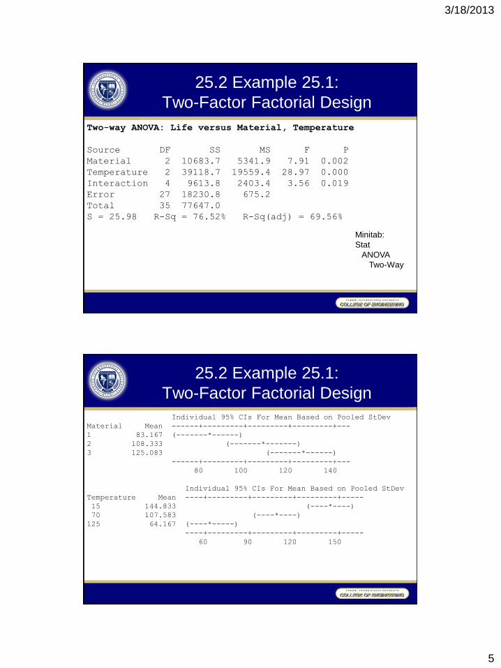
Two-way ANOVA: Life versus Material, Temperature
Source DF SS MS F P
Material 2 10683.7 5341.9 7.91 0.002
Temperature 2 39118.7 19559.4 28.97 0.000
Interaction 4 9613.8 2403.4 3.56 0.019
Error 27 18230.8 675.2
Total 35 77647.0
S = 25.98 R-Sq = 76.52% R-Sq(adj) = 69.56%
Minitab:
Stat
ANOVA
Two-Way
25.2 Example 25.1:
Two-Factor Factorial Design
Individual 95% CIs For Mean Based on Pooled StDev
Material Mean ------+---------+---------+---------+---
1 83.167 (-------*------)
2 108.333 (-------*-------)
3 125.083 (-------*------)
------+---------+---------+---------+---
80 100 120 140
Individual 95% CIs For Mean Based on Pooled StDev
Temperature Mean ----+---------+---------+---------+-----
15 144.833 (----*----)
70 107.583 (----*----)
125 64.167 (----*-----)
----+---------+---------+---------+-----
60 90 120 150
3/18/2013
6
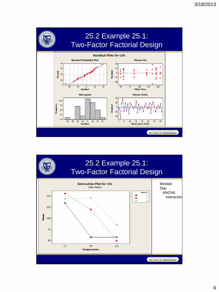
25.2 Example 25.1:
Two-Factor Factorial Design
25.2 Example 25.1:
Two-Factor Factorial Design
Minitab:
Stat
ANOVA
Interaction

3/18/2013
7
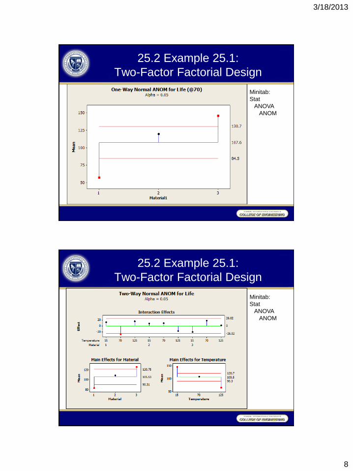
25.2 Example 25.1:
Two-Factor Factorial Design
Minitab:
Stat
ANOVA
Interaction
25.2 Example 25.1:
Two-Factor Factorial Design
Minitab:
Stat
ANOVA
Main Effects
3/18/2013
8
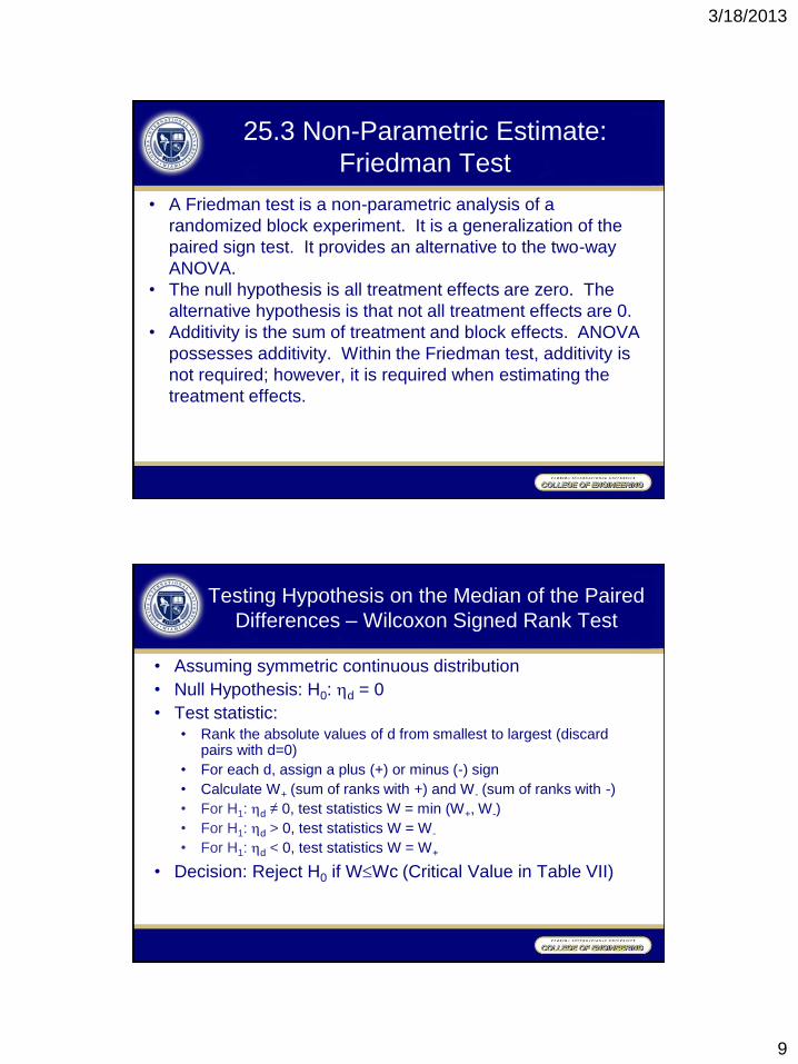
25.2 Example 25.1:
Two-Factor Factorial Design
Minitab:
Stat
ANOVA
ANOM
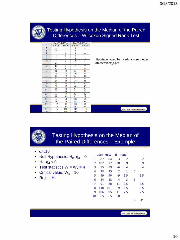
25.2 Example 25.1:
Two-Factor Factorial Design
Minitab:
Stat
ANOVA
ANOM
3/18/2013
9
• A Friedman test is a non-parametric analysis of a
randomized block experiment. It is a generalization of the
paired sign test. It provides an alternative to the two-way
ANOVA.
• The null hypothesis is all treatment effects are zero. The
alternative hypothesis is that not all treatment effects are 0.
• Additivity is the sum of treatment and block effects. ANOVA
possesses additivity. Within the Friedman test, additivity is
not required; however, it is required when estimating the
treatment effects.
25.3 Non-Parametric Estimate:
Friedman Test
Testing Hypothesis on the Median of the Paired
Differences – Wilcoxon Signed Rank Test
• Assuming symmetric continuous distribution
• Null Hypothesis: H0: d = 0
• Test statistic: • Rank the absolute values of d from smallest to largest (discard
pairs with d=0)
• For each d, assign a plus (+) or minus (-) sign
• Calculate W+ (sum of ranks with +) and W- (sum of ranks with -)
• For H1: d ≠ 0, test statistics W = min (W+, W-)
• For H1: d > 0, test statistics W = W-
• For H1: d < 0, test statistics W = W+
• Decision: Reject H0 if WWc (Critical Value in Table VII)
3/18/2013
10
Testing Hypothesis on the Median of the Paired
Differences – Wilcoxon Signed Rank Test
http://facultyweb.berry.edu/vbissonnette/
tables/wilcox_t.pdf
Testing Hypothesis on the Median of
the Paired Differences – Example
• =.10
• Null Hypothesis: H0: d = 0
• H1: d < 0
• Test statistics W = W+ = 4
• Critical value: Wc = 10
• Reject H0
Curr. New d Rank + - 1 87 84 -3 2 2 2 102 72 -30 9 9 3 95 89 -6 4 4 4 73 75 2 1 1 5 99 90 -9 5.5 5.5 6 84 88 4 3 3 7 91 80 -11 7.5 7.5 8 110 101 -9 5.5 5.5 9 106 95 -11 7.5 7.5
10 65 65 0 4 41
3/18/2013
11
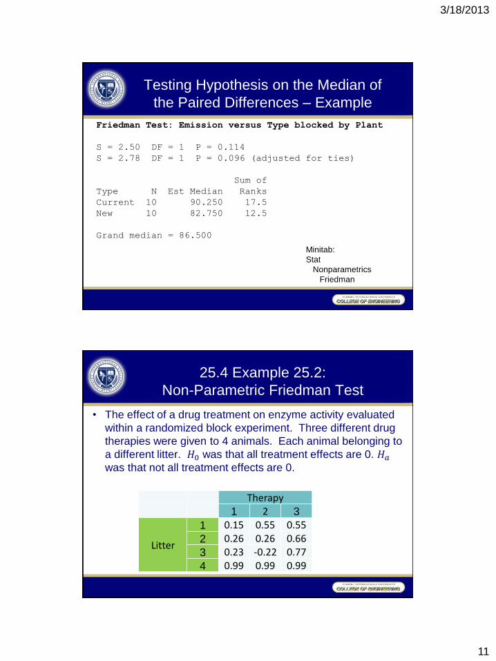
Testing Hypothesis on the Median of
the Paired Differences – Example
Minitab:
Stat
Nonparametrics
Friedman
Friedman Test: Emission versus Type blocked by Plant
S = 2.50 DF = 1 P = 0.114
S = 2.78 DF = 1 P = 0.096 (adjusted for ties)
Sum of
Type N Est Median Ranks
Current 10 90.250 17.5
New 10 82.750 12.5
Grand median = 86.500
25.4 Example 25.2:
Non-Parametric Friedman Test
• The effect of a drug treatment on enzyme activity evaluated
within a randomized block experiment. Three different drug
therapies were given to 4 animals. Each animal belonging to
a different litter. 𝐻0 was that all treatment effects are 0. 𝐻𝑎
was that not all treatment effects are 0.
Therapy
1 2 3
Litter
1 0.15 0.55 0.55
2 0.26 0.26 0.66
3 0.23 -0.22 0.77
4 0.99 0.99 0.99
3/18/2013
12
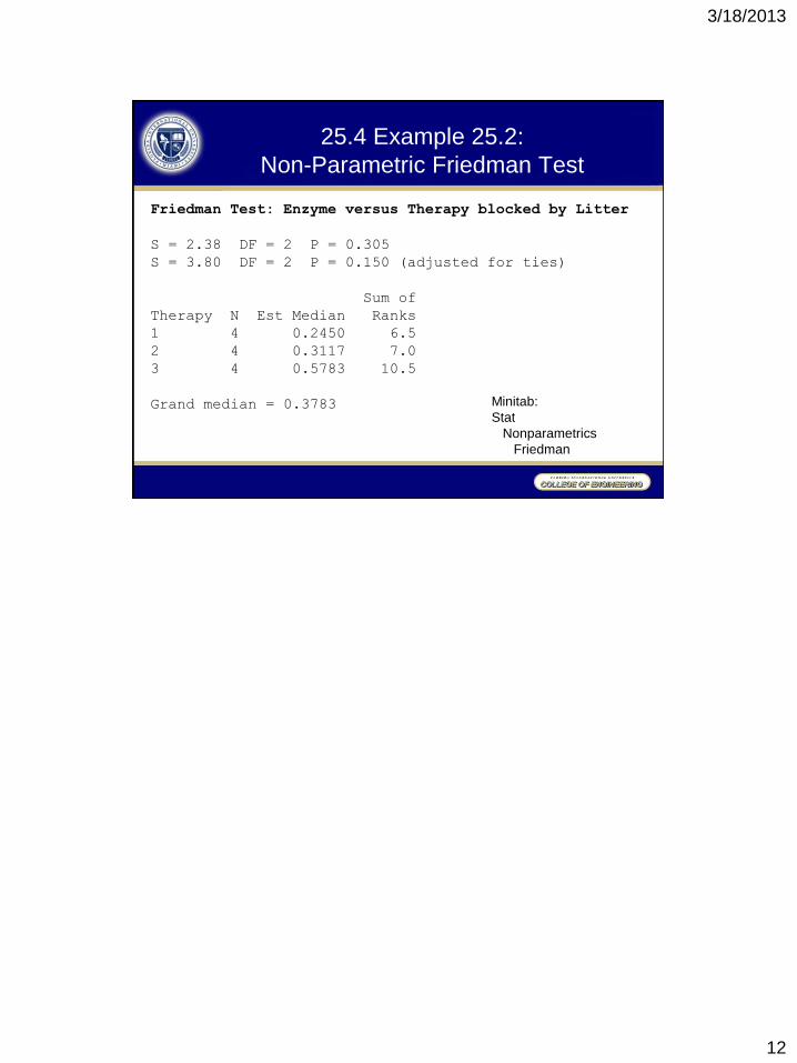
25.4 Example 25.2:
Non-Parametric Friedman Test
Minitab:
Stat
Nonparametrics
Friedman
Friedman Test: Enzyme versus Therapy blocked by Litter
S = 2.38 DF = 2 P = 0.305
S = 3.80 DF = 2 P = 0.150 (adjusted for ties)
Sum of
Therapy N Est Median Ranks
1 4 0.2450 6.5
2 4 0.3117 7.0
3 4 0.5783 10.5
Grand median = 0.3783