Embed Size (px)
DESCRIPTION
One-Way Analysis of Variance (ANOVA), II. 2011, 12, 6. Lab 19 Worksheet Q1. - PowerPoint PPT Presentation
Citation preview
One-Way Analysis of Variance (ANOVA), II
2011, 12, 6

Lab 19 Worksheet Q1
A developmental psychologist is examining problem-solving ability for grade school children. Random samples of 5-year-old, 6-year-old, and 7-year-old children are obtained with n = 3 in each sample, and problem solving is measured for each child. Do the following data indicate significant differences among the three age groups? Test with alpha = .05.

Q1. Problem-Solving Among 5-, 6-, and 7-year-olds7-year-old 6-year-old 5-year-old
5 6 0
4 4 1
6 2 2
Step 1: Form Hypotheses
H0 :
H1 :
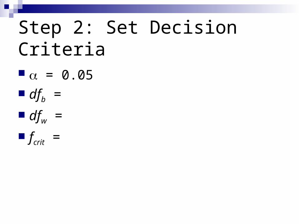
Step 2: Set Decision Criteria
= 0.05 dfb =
dfw =
fcrit =

dfB dfW 1 2 3 4 5 6 7 8 9 10
1 161.4 199.5 215.7 224.6 230.2 234.0 236.8 238.9 240.5 241.9
2 18.51 19.00 19.16 19.25 19.30 19.33 19.35 19.37 19.38 19.40
3 10.13 9.55 9.28 9.12 9.01 8.94 8.89 8.85 8.81 8.79
4 7.71 6.94 6.59 6.39 6.26 6.16 6.09 6.04 6.00 5.96
5 6.61 5.79 5.41 5.19 5.05 4.95 4.88 4.82 4.77 4.74
6 5.99 5.14 4.76 4.53 4.39 4.28 4.21 4.15 4.10 4.06
7 5.59 4.74 4.35 4.12 3.97 3.87 3.79 3.73 3.68 3.64
8 5.32 4.46 4.07 3.84 3.69 3.58 3.50 3.44 3.39 3.35
9 5.12 4.26 3.86 3.63 3.48 3.37 3.29 3.23 3.18 3.14
10 4.96 4.10 3.71 3.48 3.33 3.22 3.14 3.07 3.02 2.98
11 4.84 3.98 3.59 3.36 3.20 3.09 3.01 2.95 2.90 2.85
12 4.75 3.89 3.49 3.26 3.11 3.00 2.91 2.85 2.80 2.75
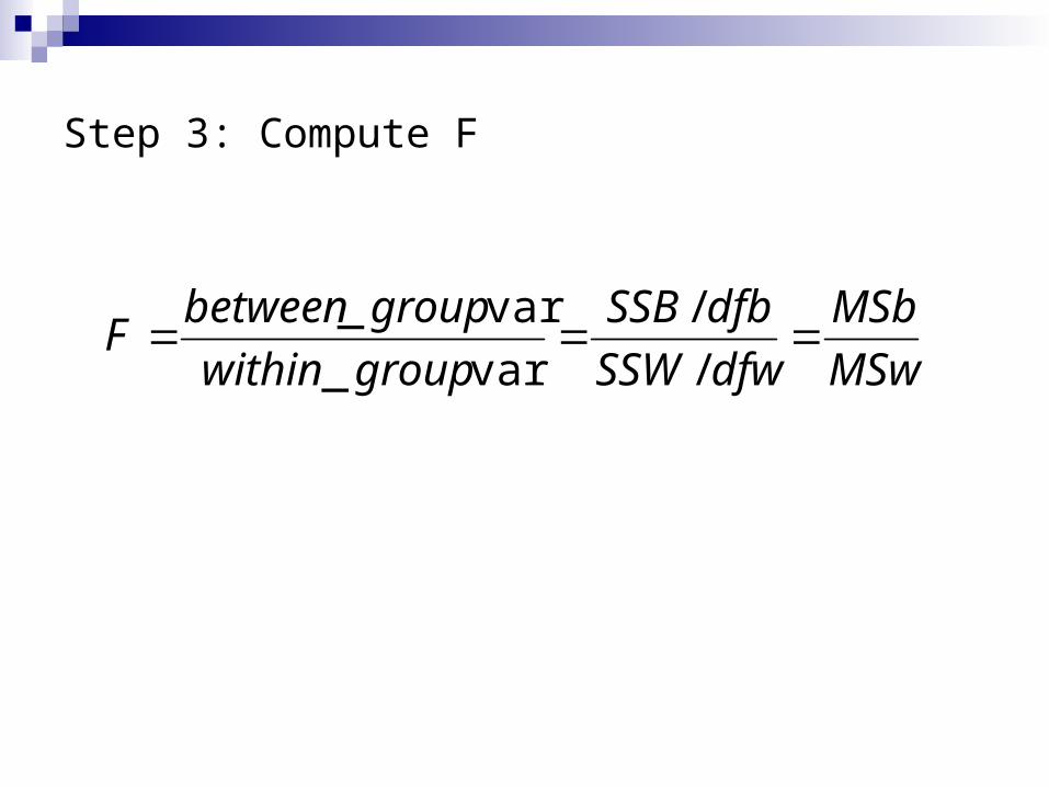
Step 3: Compute F
MSw
MSb
dfwSSW
dfbSSB
groupwithin
groupbetweenF
/
/
var_
var_

7-year-old (n1 = 3) 6-year-old (n2 = 3) 5-year-old (n3 = 3)
Y1 Y12 Y2 Y2
2 Y3 Y32
5 25 6 36 0 0
4 16 4 16 1 1
6 36 2 4 2 4
Y1=15 Y12=77 Y2=12 Y2
2= 56 Y3=3 Y32=5
Y1 = 5 SSW1 = 2 Y2 = 4 SSW2 = 8 Y3 = 1 SSW3 = 2
1
212
11
)(
n
YYSSW
2
222
22
)(
n
YYSSW
3
232
33
)(
n
YYSSW
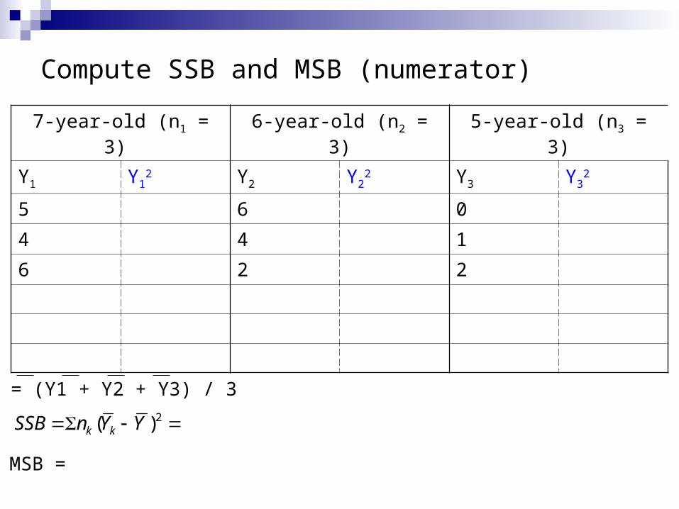
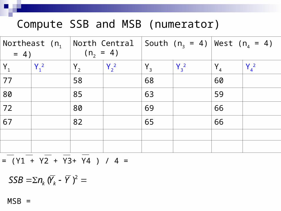
Compute SSB and MSB (numerator)
2)( YYnSSB kk
MSB =
7-year-old (n1 = 3) 6-year-old (n2 = 3) 5-year-old (n3 = 3)
Y1 Y12 Y2 Y2
2 Y3 Y32
5 6 0
4 4 1
6 2 2
Y = (Y1 + Y2 + Y3) / 3
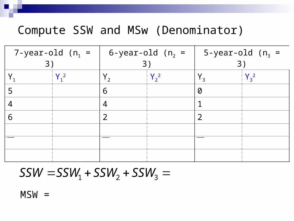
Compute SSW and MSw (Denominator)
7-year-old (n1 = 3) 6-year-old (n2 = 3) 5-year-old (n3 = 3)
Y1 Y12 Y2 Y2
2 Y3 Y32
5 6 0
4 4 1
6 2 2
321 SSWSSWSSWSSW
MSW =

Step 4: Create ANOVA Source TableSource SS df MS F
Between 26 2 13 6.5
Within 12 6 2
Total 38 8

Step 5. Make Decision
Compare Fobs to Fcrit.
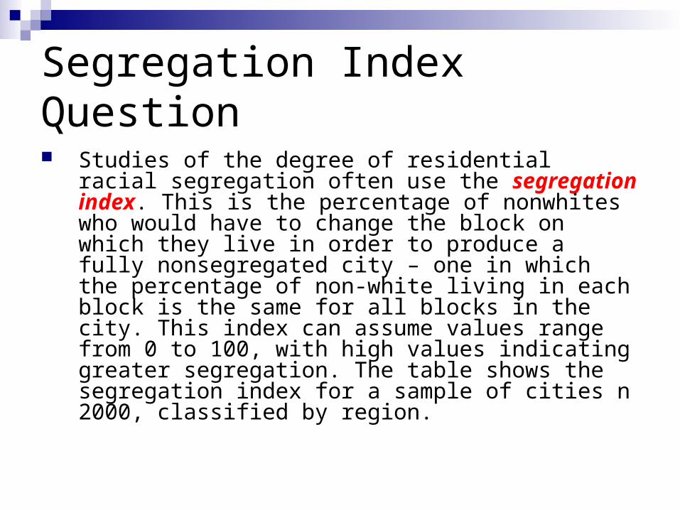
Segregation Index Question
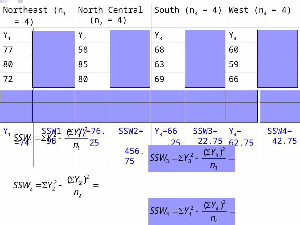
Studies of the degree of residential racial segregation often use the segregation index. This is the percentage of nonwhites who would have to change the block on which they live in order to produce a fully nonsegregated city – one in which the percentage of non-white living in each block is the same for all blocks in the city. This index can assume values range from 0 to 100, with high values indicating greater segregation. The table shows the segregation index for a sample of cities n 2000, classified by region.
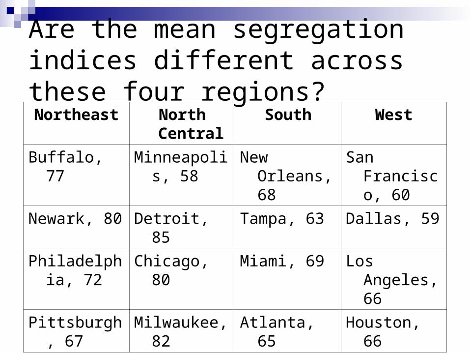
Are the mean segregation indices different across these four regions?
Northeast North Central South West
Buffalo, 77 Minneapolis, 58 New Orleans, 68 San Francisco, 60
Newark, 80 Detroit, 85 Tampa, 63 Dallas, 59
Philadelphia, 72 Chicago, 80 Miami, 69 Los Angeles, 66
Pittsburgh, 67 Milwaukee, 82 Atlanta, 65 Houston, 66
Step 1: Form Hypotheses
H0 :
H1 :

Step 2: Set Decision Criteria
Alpha = 0.05 dfb = dfw = Fcrit =
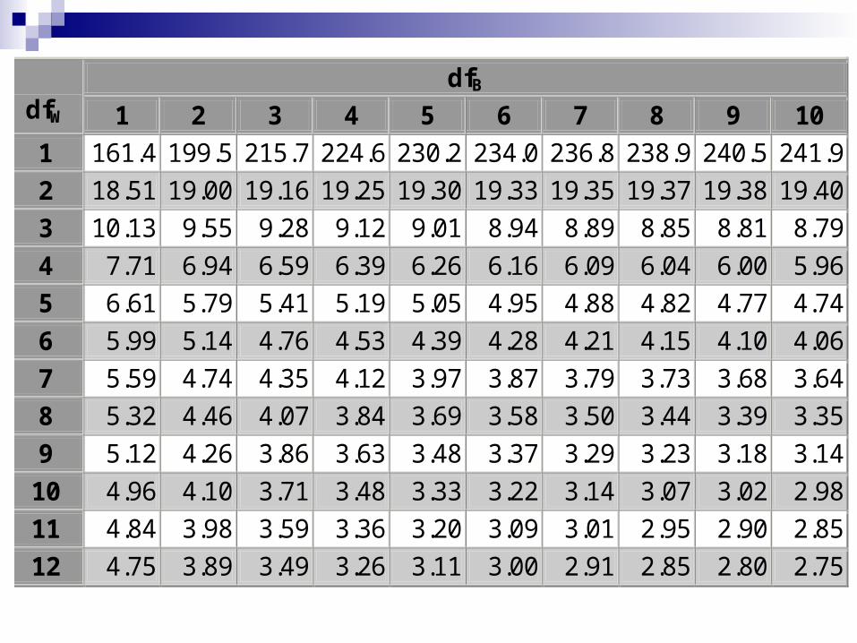
dfB dfW 1 2 3 4 5 6 7 8 9 10
1 161.4 199.5 215.7 224.6 230.2 234.0 236.8 238.9 240.5 241.9
2 18.51 19.00 19.16 19.25 19.30 19.33 19.35 19.37 19.38 19.40
3 10.13 9.55 9.28 9.12 9.01 8.94 8.89 8.85 8.81 8.79
4 7.71 6.94 6.59 6.39 6.26 6.16 6.09 6.04 6.00 5.96
5 6.61 5.79 5.41 5.19 5.05 4.95 4.88 4.82 4.77 4.74
6 5.99 5.14 4.76 4.53 4.39 4.28 4.21 4.15 4.10 4.06
7 5.59 4.74 4.35 4.12 3.97 3.87 3.79 3.73 3.68 3.64
8 5.32 4.46 4.07 3.84 3.69 3.58 3.50 3.44 3.39 3.35
9 5.12 4.26 3.86 3.63 3.48 3.37 3.29 3.23 3.18 3.14
10 4.96 4.10 3.71 3.48 3.33 3.22 3.14 3.07 3.02 2.98
11 4.84 3.98 3.59 3.36 3.20 3.09 3.01 2.95 2.90 2.85
12 4.75 3.89 3.49 3.26 3.11 3.00 2.91 2.85 2.80 2.75

Step 3: Compute F
MSw
MSb
dfwSSW
dfbSSB
groupwithin
groupbetweenF
/
/
var_
var_
Northeast (n1 = 4) North Central (n2 = 4) South (n3 = 4) West (n4 = 4)
Y1 Y12 Y2 Y2
2 Y3 Y32 Y4 Y4
2
77 5929 58 3364 68 4624 60 3600
80 6400 85 7225 63 3969 59 3481
72 5184 80 6400 69 4761 66 4356
67 4489 82 6724 65 4225 66 4356Y1=296 Y1
2=22002 Y2= 305 Y22=23713 Y3=265 Y3
2=17579 Y4=251 Y42=15793
Y1 =74 SSW1 = 98
Y2=76.25 SSW2= 456.75
Y3=66.25
SSW3= 22.75
Y4=62.75
SSW4= 42.75
1
212
11
)(
n
YYSSW
2
222
22
)(
n
YYSSW
4
242
44
)(
n
YYSSW
3
232
33
)(
n
YYSSW
2)( YYnSSB kk
Compute SSB and MSB (numerator)
MSB =
Y = (Y1 + Y2 + Y3+ Y4 ) / 4 =
Northeast (n1 = 4) North Central (n2 = 4) South (n3 = 4) West (n4 = 4)
Y1 Y12 Y2 Y2
2 Y3 Y32 Y4 Y4
2
77 58 68 60
80 85 63 59
72 80 69 66
67 82 65 66

Compute SSW and MSw (Denominator)
4321 SSWSSWSSWSSWSSW
MSW =
Northeast (n1 = 4) North Central (n2 = 4) South (n3 = 4) West (n4 = 4)
Y1 Y12 Y2 Y2
2 Y3 Y32 Y4 Y4
2
77 58 68 60
80 85 63 59
72 80 69 66
67 82 65 66
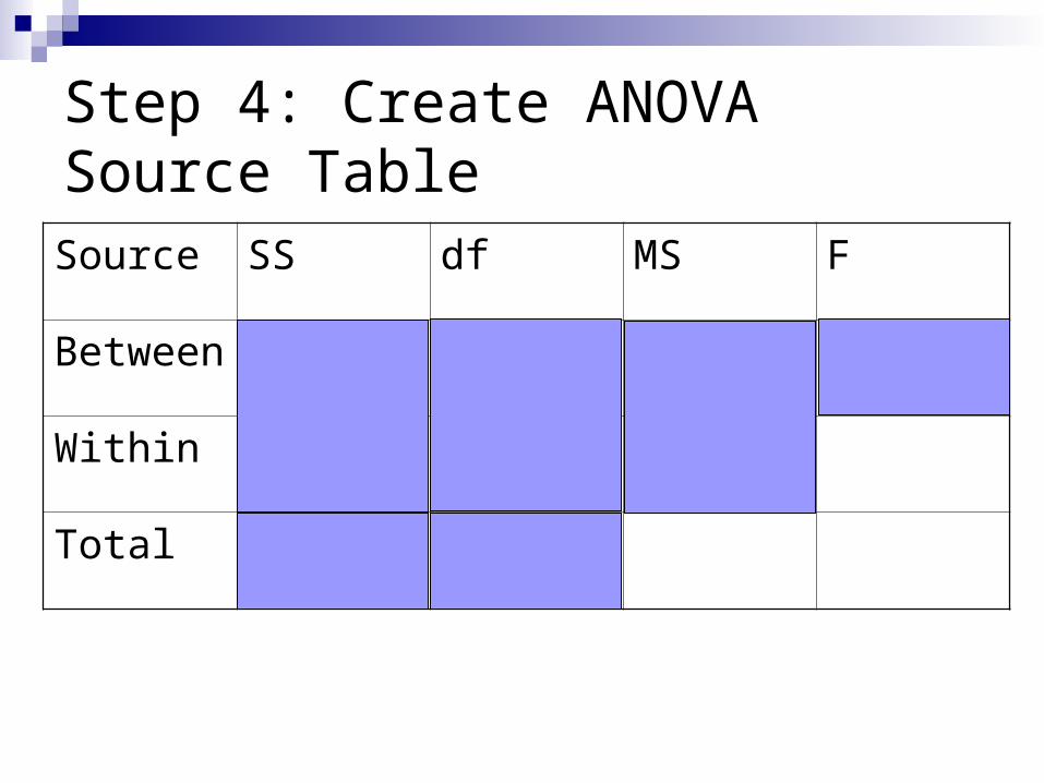
Step 4: Create ANOVA Source TableSource SS df MS F
Between 486.19 3 162.06 3.14
Within 620.25 12 51.69
Total 1106.44 15
Step 5. Make Decision
Compare Fobs to Fcrit.