2 Way Analysis of Variance (ANOVA)

Peter Shaw

RU

ANOVA - a recapitulation.

This is a parametric test, examining whether the means differ between 2 or more populations.

It generates a test statistic F, which can be thought of as a signal:noise ratio. Thus large Values of F indicate a high degree of pattern within the data and imply rejection of H0.

It is thus similar to the t test - in fact ANOVA on 2 groups is equivalent to a t test [F = t2 ]

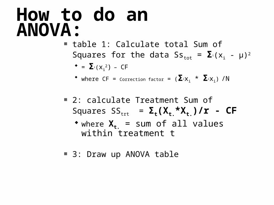
How to do an ANOVA: table 1: Calculate total Sum of Squares for the

data Sstot = Σi(xi - μ)2

= Σi(xi2) – CF

where CF = Correction factor = (Σixi * Σixi) /N

2: calculate Treatment Sum of Squares SStrt = Σt(Xt.*Xt.)/r - CF where Xt. = sum of all values within

treatment t

3: Draw up ANOVA table

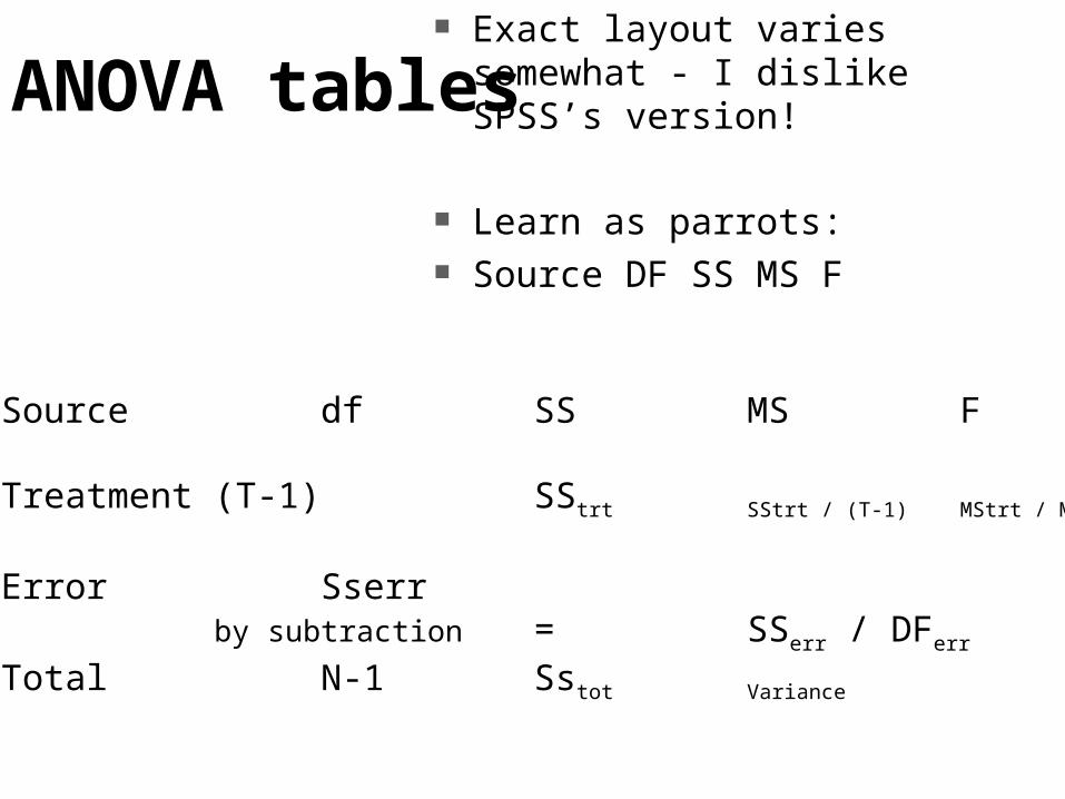
ANOVA tables Exact layout varies somewhat

- I dislike SPSS’s version!

Learn as parrots: Source DF SS MS F

Source df SS MS F

Treatment (T-1) SStrt SStrt / (T-1) MStrt / MSerr

Error Sserrby subtraction = SSerr / DFerr

Total N-1 Sstot Variance

One way ANOVA’s limitations

This technique is only applicable when there is one treatment used.

Note that the one treatment can be at 3, 4,… many levels. Thus fertiliser trials with 10 concentrations of fertiliser could be analysed this way, but a trial of BOTH fertiliser and insecticide could not.

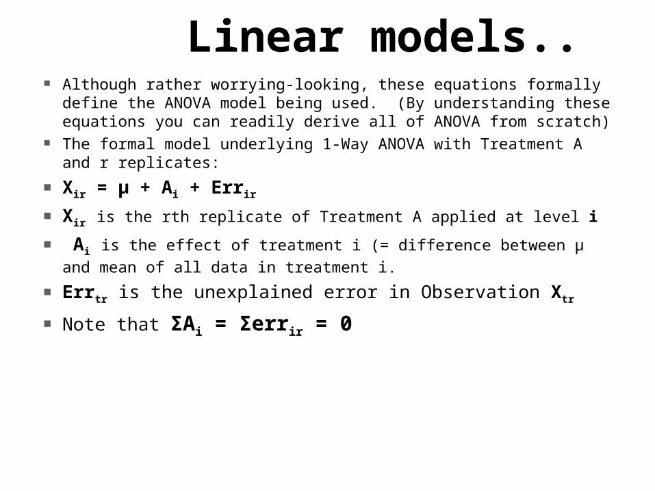
Linear models.. Although rather worrying-looking, these equations formally define the

ANOVA model being used. (By understanding these equations you can readily derive all of ANOVA from scratch)

The formal model underlying 1-Way ANOVA with Treatment A and r replicates:

Xir = μ + Ai + Errir

Xir is the rth replicate of Treatment A applied at level i

Ai is the effect of treatment i (= difference between μ and mean of all data in

treatment i.

Errtr is the unexplained error in Observation Xtr

Note that ΣAi = Σerrir = 0

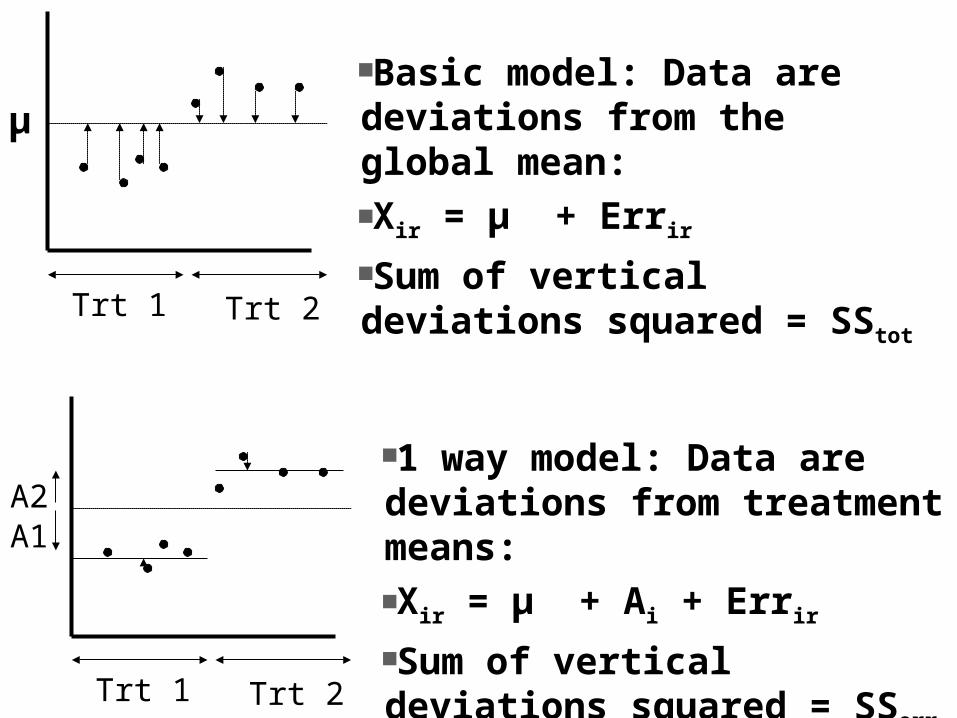
μ

Trt 1 Trt 2

Basic model: Data are deviations from the global mean:Xir = μ + Errir

Sum of vertical deviations squared = SStot

Trt 1 Trt 2

1 way model: Data are deviations from treatment means:Xir = μ + Ai + Errir

Sum of vertical deviations squared = SSerr

A1A2

μ

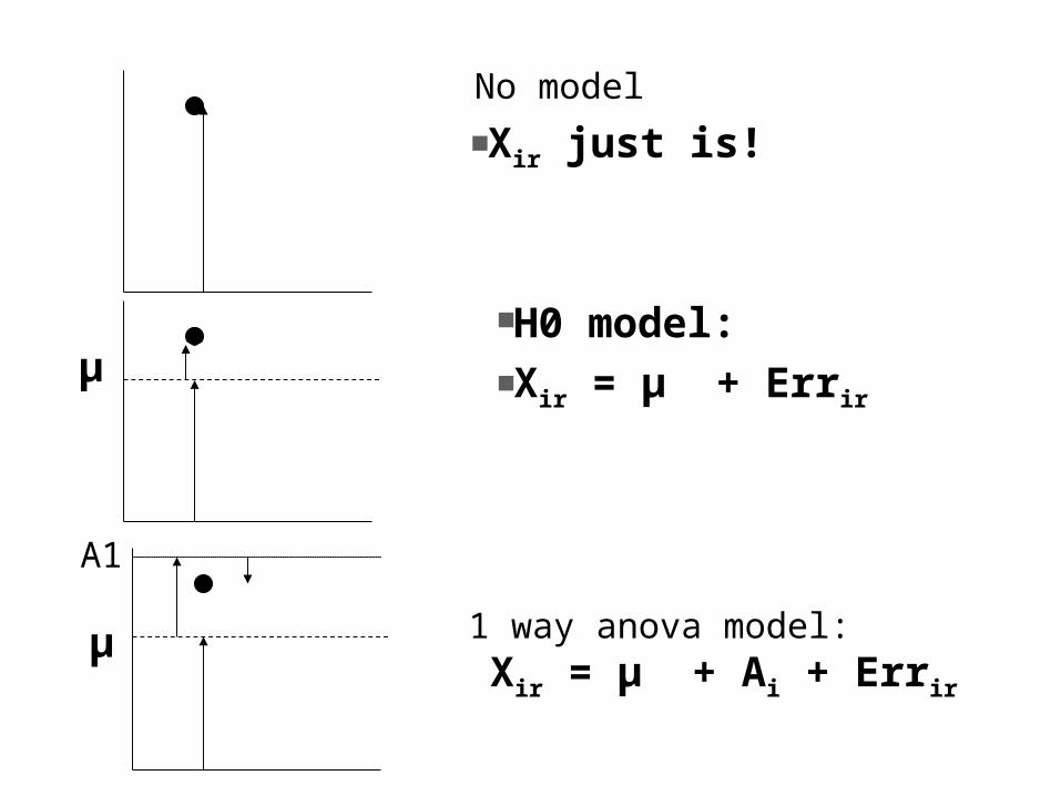
μ

A1

No model

Xir just is!

H0 model:Xir = μ + Errir

1 way anova model: Xir = μ + Ai + Errir

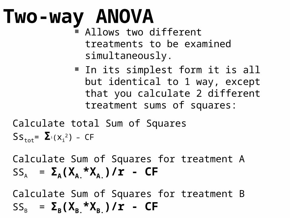
Two-way ANOVA Allows two different treatments to

be examined simultaneously. In its simplest form it is all but

identical to 1 way, except that you calculate 2 different treatment sums of squares:

Calculate total Sum of Squares Sstot= Σi(xi

2) – CF

Calculate Sum of Squares for treatment ASSA = ΣA(XA.*XA.)/r - CF

Calculate Sum of Squares for treatment BSSB = ΣB(XB.*XB.)/r - CF

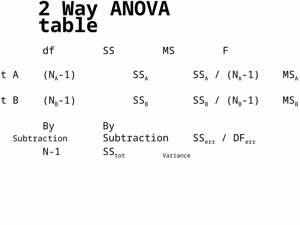
2 Way ANOVA table

Source df SS MS F

Treatment A (NA-1) SSA SSA / (NA-1) MSA / MSerr

Treatment B (NB-1) SSB SSB / (NB-1) MSB / MSerr

Error By BySubtraction Subtraction SSerr / DFerr

Total N-1 SStot Variance

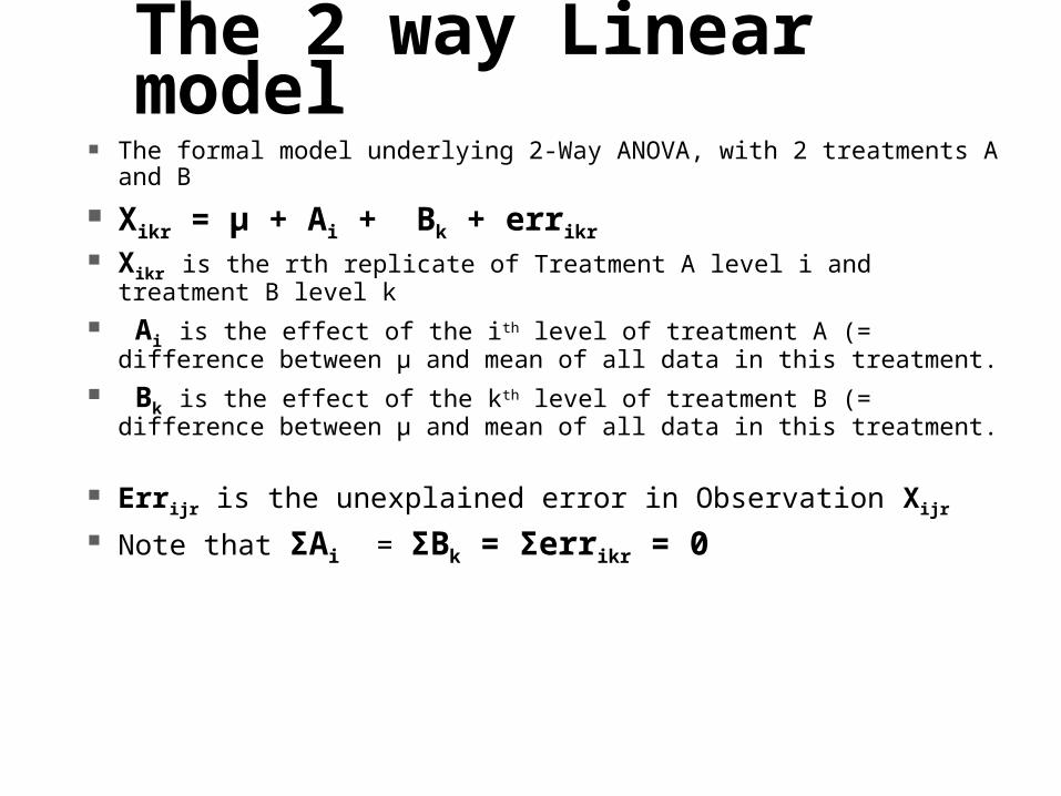
The 2 way Linear model The formal model underlying 2-Way ANOVA, with 2 treatments A and B

Xikr = μ + Ai + Bk + errikr Xikr is the rth replicate of Treatment A level i and treatment B level k Ai is the effect of the ith level of treatment A (= difference between μ and

mean of all data in this treatment. Bk is the effect of the kth level of treatment B (= difference between μ and

mean of all data in this treatment.

Errijr is the unexplained error in Observation Xijr

Note that ΣAi = ΣBk = Σerrikr = 0

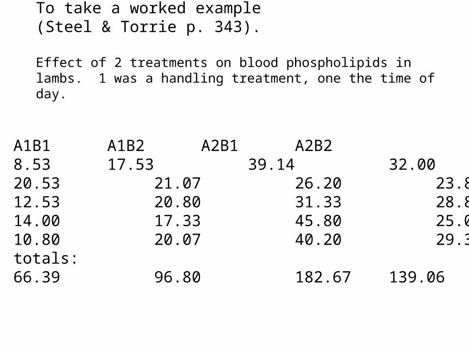
To take a worked example (Steel & Torrie p. 343).

Effect of 2 treatments on blood phospholipids in lambs. 1 was a handling treatment, one the time of day.

A1B1 A1B2 A2B1 A2B28.53 17.53 39.14 32.0020.53 21.07 26.20 23.8012.53 20.80 31.33 28.8714.00 17.33 45.80 25.0610.80 20.07 40.20 29.33totals:66.39 96.80 182.67 139.06

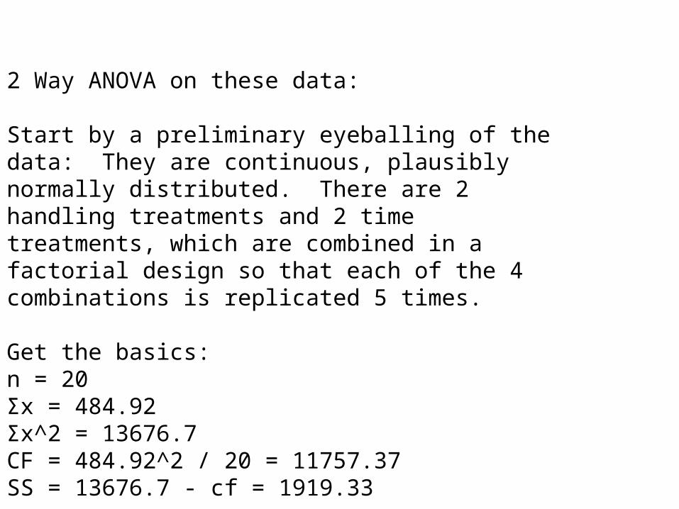
2 Way ANOVA on these data:

Start by a preliminary eyeballing of the data: They are continuous, plausibly normally distributed. There are 2 handling treatments and 2 time treatments, which are combined in a factorial design so that each of the 4 combinations is replicated 5 times.

Get the basics:n = 20Σx = 484.92Σx^2 = 13676.7CF = 484.92^2 / 20 = 11757.37SS = 13676.7 - cf = 1919.33

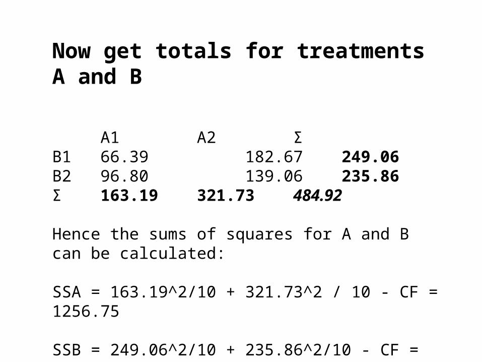
Now get totals for treatments A and B

A1 A2 ΣB1 66.39 182.67 249.06B2 96.80 139.06 235.86Σ 163.19 321.73 484.92

Hence the sums of squares for A and B can be calculated:

SSA = 163.19^2/10 + 321.73^2 / 10 - CF = 1256.75

SSB = 249.06^2/10 + 235.86^2/10 - CF = 8.712

A aloneSource Df SS MS FA 1 1256.75 1256.75 34.14**error 18 662.58 36.81total 19 1919.33

B aloneSource Df SS MS FB 1 8.71 8.71 0.08 NSerror 18 1910.62 106.15total 19 1919.33

Pooled (the correct format)Source Df SS MS FA 1 1256.75 1256.75 32.67**B 1 8.71 8.71 0.24NSerror 17 653.87 38.86total 19 1919.33

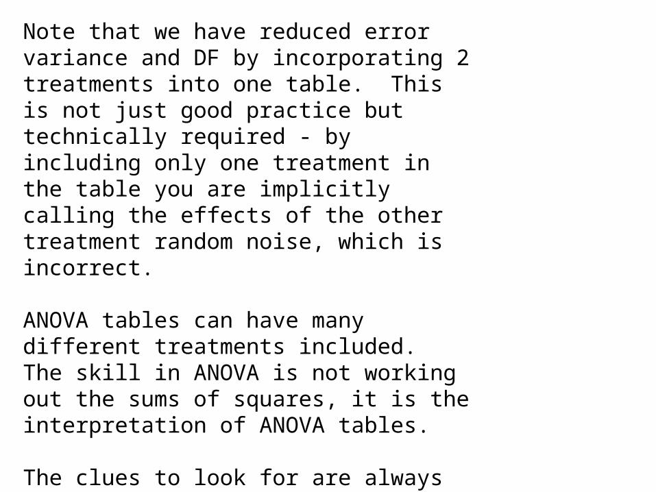
Note that we have reduced error variance and DF by incorporating 2 treatments into one table. This is not just good practice but technically required - by including only one treatment in the table you are implicitly calling the effects of the other treatment random noise, which is incorrect.

ANOVA tables can have many different treatments included. The skill in ANOVA is not working out the sums of squares, it is the interpretation of ANOVA tables.

The clues to look for are always in the DF column. A treatment with N levels has N-1 DF - this always applies and allows you to infer the model a researcher was using to analyse data.

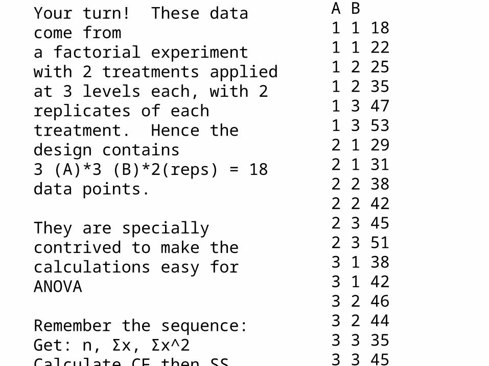
A B1 1 181 1 221 2 251 2 351 3 471 3 532 1 292 1 312 2 382 2 422 3 452 3 513 1 383 1 423 2 463 2 443 3 353 3 45

Your turn! These data come froma factorial experiment with 2 treatments applied at 3 levels each, with 2 replicates of each treatment. Hence the design contains3 (A)*3 (B)*2(reps) = 18 data points.

They are specially contrived to make the calculations easy for ANOVA

Remember the sequence:Get: n, Σx, Σx^2Calculate CF then SStot

Get the totals for each treatment: A1, A2, A3, B1, B2 and B3 hence get SSA and SSB

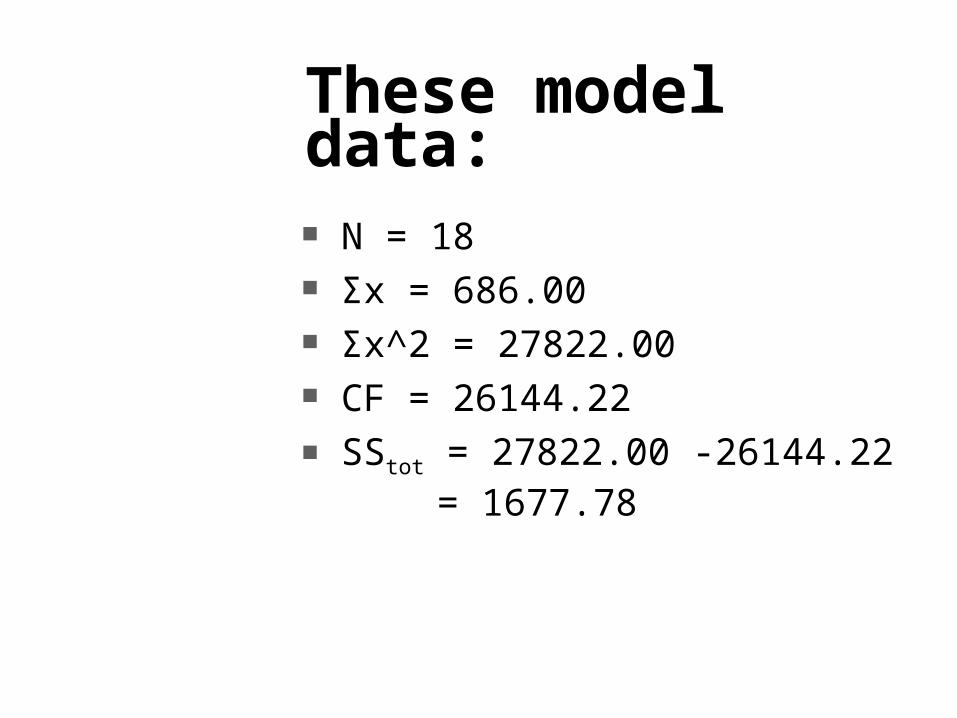
These model data:

N = 18 Σx = 686.00 Σx^2 = 27822.00 CF = 26144.22 SStot = 27822.00 -26144.22

= 1677.78

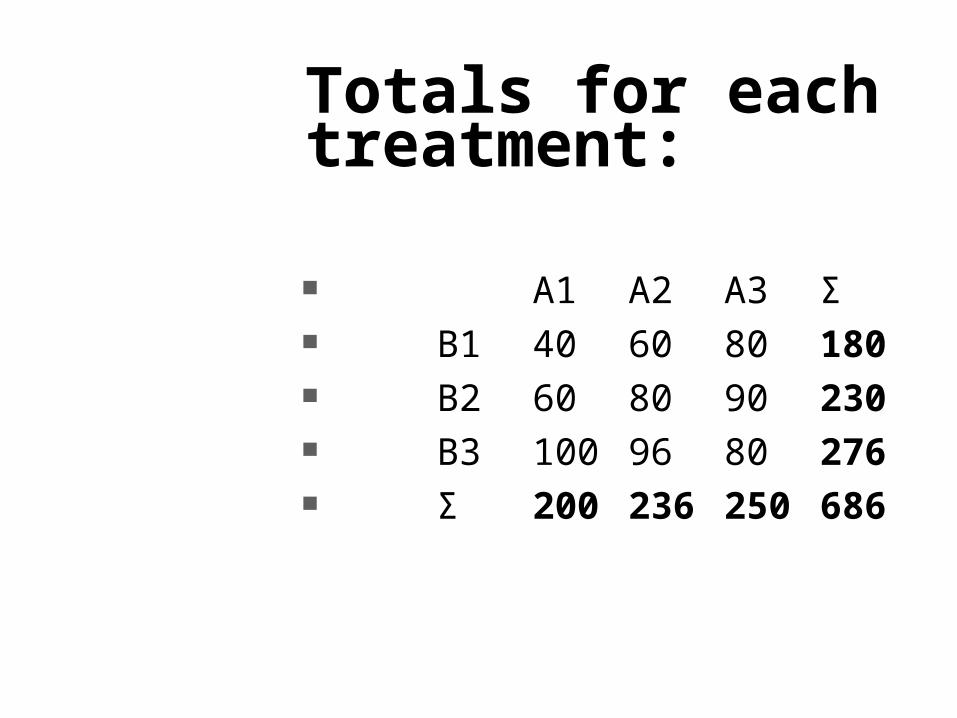
Totals for each treatment:

A1 A2 A3 Σ B1 40 60 80 180 B2 60 80 90 230 B3 100 96 80 276 Σ 200 236 250 686

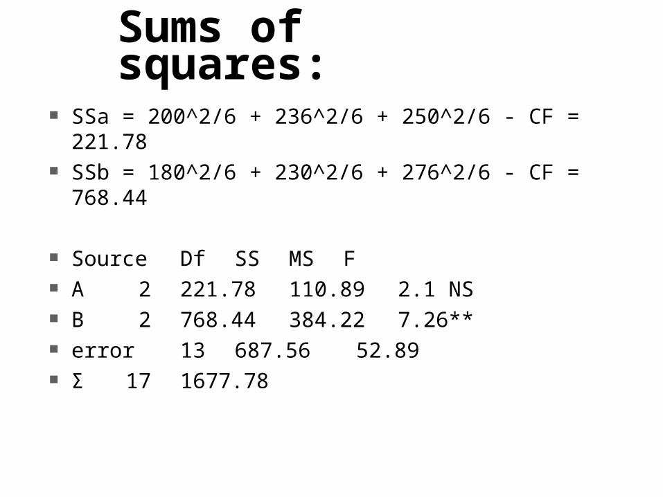
Sums of squares: SSa = 200^2/6 + 236^2/6 + 250^2/6 - CF = 221.78 SSb = 180^2/6 + 230^2/6 + 276^2/6 - CF = 768.44

Source Df SS MS F A 2 221.78 110.89 2.1 NS B 2 768.44 384.22 7.26** error 13 687.56 52.89 Σ 17 1677.78

Interaction terms We now meet a unique, powerful feature of ANOVA. It can examine data for interactions

between treatments - synergism or antagonism.

No other test allows this, while in ANOVA it is a standard feature of any 2 way table.

Note that this interaction analysis is only valid if the design is perfectly balanced. Unequal replication or missing data points make this invalid (unlike 1 way, which is robust to imbalance).

Synergism and antagonism

Some treatments intensify each others’ effects: The classic examples come from pharmacology. Alcohol alone is lethal at the 20-40 unit range.

Barbiturates are lethal. Together they are a vastly more lethal combination, as the 2 drugs synergise. (In fact most sedatives and depressants show similar dangerous synergism).

In ecology, SO2 + NO2 is more damaging than the additive effects of each gas alone - a synergism.

Antagonism.

is the opposite - 2 treatments nullifying each other.

Drought antagonises effects of air pollution on plants, as drought leads to closed stomata excluding the noxious gas.

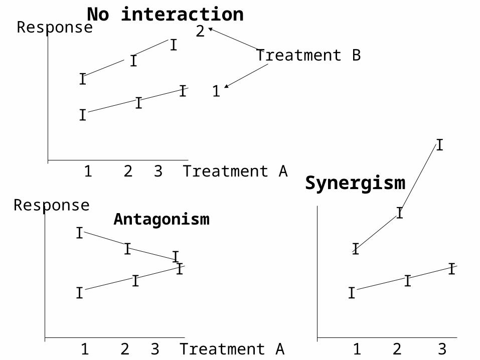
1 2 3 Treatment A

II

I 1

Treatment B

Response

1 2 3 Treatment A

II

I

Response

1 2 3

II

I

II

I2

No interaction

I

I

I

Synergism

II I

Antagonism

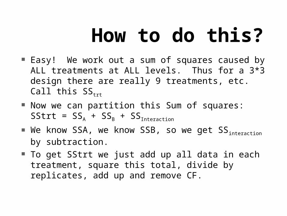
How to do this? Easy! We work out a sum of squares caused by ALL

treatments at ALL levels. Thus for a 3*3 design there are really 9 treatments, etc. Call this SStrt

Now we can partition this Sum of squares: SStrt = SSA + SSB + SSInteraction

We know SSA, we know SSB, so we get SSinteraction by subtraction.

To get SStrt we just add up all data in each treatment, square this total, divide by replicates, add up and remove CF.

For the lamb blood data:

We have 4 separate treatments: A1B1, A1B2, A2B1, A2B2

The data within these 4 groups add to: 66.39, 182.67, 96.80, 139.06. There are 5 replicates

SStrt = 66.39^2/5 + 182.67^2/5 + 96.8^2/5 + 139.06^2/5 - CF = 1539.407

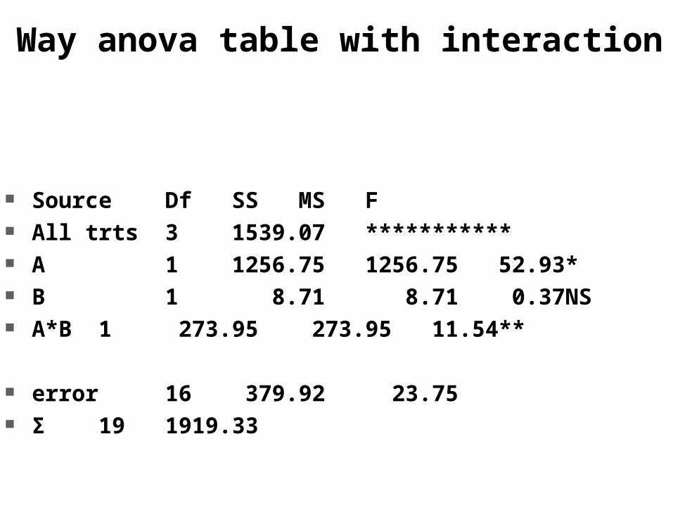
Source Df SS MS F All trts 3 1539.07 *********** A 1 1256.75 1256.75 52.93* B 1 8.71 8.71 0.37NS A*B 1 273.95 273.95 11.54**

error 16 379.92 23.75 Σ 19 1919.33

2 Way anova table with interaction

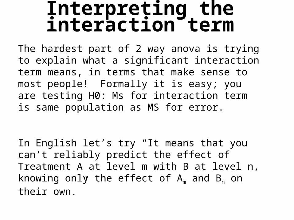
Interpreting the interaction term

The hardest part of 2 way anova is trying to explain what a significant interaction term means, in terms that make sense to most people! Formally it is easy; you are testing H0: Ms for interaction term is same population as MS for error.

In English let’s try “It means that you can’t reliably predict the effect of Treatment A at level m with B at level n, knowing only the effect of Am and Bn on their own.”

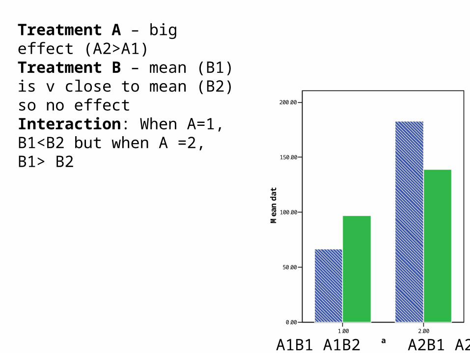
Treatment A – big effect (A2>A1)Treatment B – mean (B1) is v close to mean (B2) so no effectInteraction: When A=1, B1<B2 but when A =2, B1> B2

1.00 2.00

a

0.00

50.00

100.00

150.00

200.00

Me

an

dat

b1.00

2.00

A1B1 A1B2 A2B1 A2B2