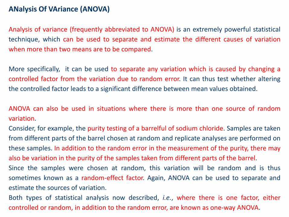
ANalysis Of VAriance (ANOVA)

Analysis of variance (frequently abbreviated to ANOVA) is an extremely powerful statisticaltechnique, which can be used to separate and estimate the different causes of variationwhen more than two means are to be compared.

More specifically, it can be used to separate any variation which is caused by changing acontrolled factor from the variation due to random error. It can thus test whether alteringthe controlled factor leads to a significant difference between mean values obtained.

ANOVA can also be used in situations where there is more than one source of randomvariation.Consider, for example, the purity testing of a barrelful of sodium chloride. Samples are takenfrom different parts of the barrel chosen at random and replicate analyses are performed onthese samples. In addition to the random error in the measurement of the purity, there mayalso be variation in the purity of the samples taken from different parts of the barrel.Since the samples were chosen at random, this variation will be random and is thussometimes known as a random-effect factor. Again, ANOVA can be used to separate andestimate the sources of variation.Both types of statistical analysis now described, i.e., where there is one factor, eithercontrolled or random, in addition to the random error, are known as one-way ANOVA.

Let us suppose that 13 different groups of students measured the enthalpy variation relatedto HCl neutralization with NaOH, each of them making 5 replicated measurements.Mean values and variances for each group are easily calculated:

Here the statistical problem is represented by the comparison of the 13 mean values.

Group x1 x2 x3 x4 x5 x s2

1 56.9 59.2 56.3 58.0 56.9 57.46 1.32

2 53.8 55.4 58.0 59.6 55.5 56.46 5.34

3 58.4 55.0 55.7 56.6 57.2 56.58 1.74

4 58.0 56.4 57.6 57.5 55.0 56.90 1.48

5 57.7 58.5 58.9 57.8 57.4 58.06 0.38

6 54.8 56.4 55.2 60.3 57.1 56.76 4.76

7 57.1 60.4 58.9 55.5 54.7 57.32 5.55

8 58.6 57.8 58.0 55.5 55.6 57.10 2.09

9 58.9 59.8 60.0 57.1 56.4 58.44 2.61

10 59.5 57.7 60.0 57.6 56.8 58.32 1.86

11 57.2 58.2 57.4 55.7 59.1 57.52 1.60

12 55.4 56.1 57.7 56.9 59.2 57.06 2.17

13 55.1 56.8 55.7 61.6 58.3 57.50 6.74

In principle, one could make pairwise comparisons between the 13 mean values using a t-test.

However, if a significance level α (Type I error) is considered for each test, it can bedemonstrated that the error rate related to the family of data (the ensemble of groups),called Family Wise (FW) error rate, is given by:

αFW = 1- (1 - α )c

where c is the number of comparisons to be made.

Indeed, if two independent hypothesis tests are considered, each at a significance level α, the probability that neither is affected by Type I error is (1-α)2

Consequently, the probability that at least one test is affected by Type I error is:

α2 = 1 - (1- α)2

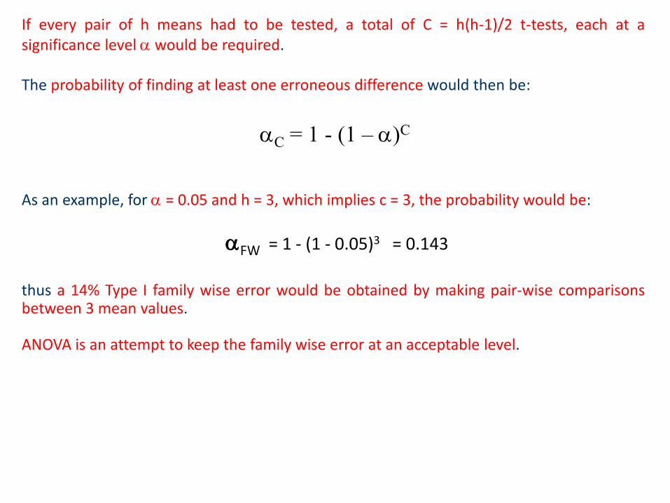
If every pair of h means had to be tested, a total of C = h(h-1)/2 t-tests, each at asignificance level α would be required.

The probability of finding at least one erroneous difference would then be:

As an example, for α = 0.05 and h = 3, which implies c = 3, the probability would be:

thus a 14% Type I family wise error would be obtained by making pair-wise comparisonsbetween 3 mean values.

ANOVA is an attempt to keep the family wise error at an acceptable level.

αFW = 1 - (1 - 0.05)3 = 0.143

αC = 1 - (1 – α)C

The table of data shown before can be generalized, indicating with i the different groups andwith j the different replicates in each group:

X11 X12 …… X1j ……. X1n

X21 X2,2 …… X2j ……. X2n

……. ……. ……. ……. …… …..Xi1 Xi2 …… Xij ……. Xin

……. …… …… ….. ……. ……Xh1 Xh2 …… Xhj ……. Xhn

∼ N(µ1 ,σ2)∼ N(µ2 ,σ2)

……∼ N(µi ,σ2)

……∼ N(µh ,σ2)

i

jGroup 1Group 2

……Group i

……Group h

Xij indicates the j-th replicate of the i-th groupn is the number of replicates (in the specific case n is the same for all groups)h is the number of groupsN = n × h is the total number of data

The basic assumption is that data in each group are extracted from a normal population witha specific mean but with the same variance as that of other groups.

We may describe the observations in Table 1 by the linear statistical model (known aseffects model):

Xij = µ + αi + εiji=1,2,…,hj=1,2,…,n

where:

Xij is a random variable denoting the (ij)th observation µ is a parameter common to all groups (treatments) called the overall mean αi is a parameter associated with the i-th group, called the i-th group effect εij is a random error component.

Note that the model could have been written according to the so-called means model:

Xij = µi + εiji=1,2,…,hj=1,2,…,n

where:µi = µ + αi is the mean of the ith treatment.

Equation 1

In this form of the model, each group defines a population that has mean µi, consisting ofthe overall mean µ plus an effect αi, that is specific of that particular group.

As shown in the following figure, referred to the case in which all αi are different from 0,the basic assumption is that errors εij are normally and independently distributed withmean zero and variance σ2.

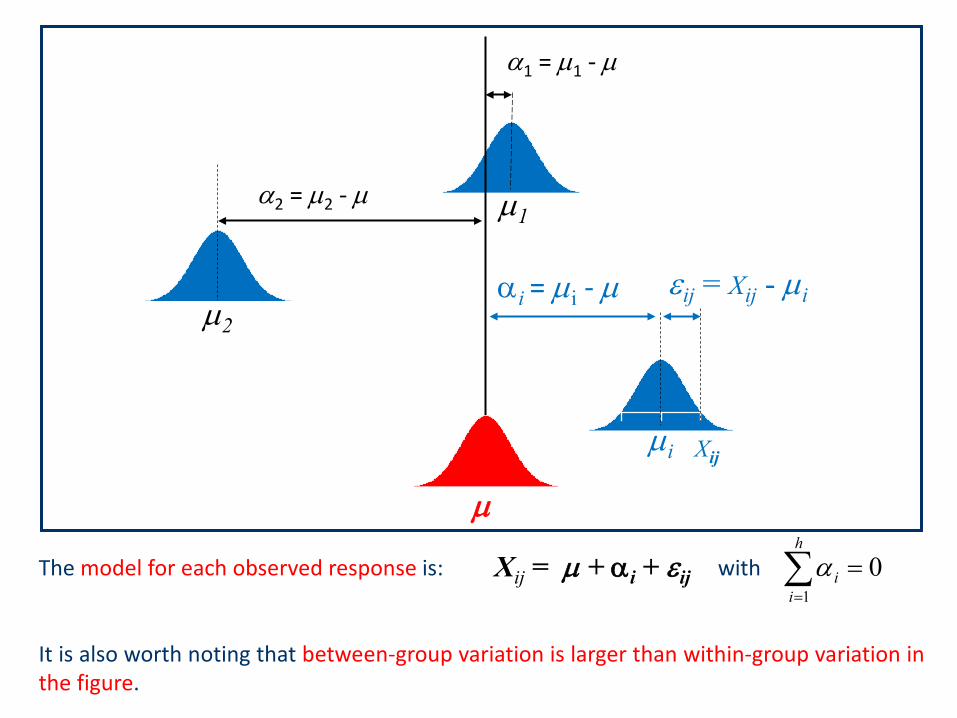
α2 = µ2 - µ

µ2

µ

µ1

α1 = µ1 - µ

εij = Xij - µiαi = µi - µ

Xijµi

Xij = µ + αi + εij 01

=∑=

h

iiαThe model for each observed response is: with

It is also worth noting that between-group variation is larger than within-group variation inthe figure.

µ1=µ2=…=µi = …= µh =µ

εij = Xij - µi

µ1

µ2

µi

µ

Xij

In the case represented by the following figure, all αi are equal to 0, which means that all µiare equal.

Equation 1:

is the underlying model for a single-factor experiment. Furthermore, since we require thatthe observations are taken in random order and that the environment in which thetreatments are used is as uniform as possible, this design is called a completely randomizedexperimental design.

Xij = µ + αi + εiji=1,2,…,hj=1,2,…,n

Since we are interested in testing the equality of the h group/treatment means:

the null (H0) and the alternative (H1) hypotheses can be formulated as follows:

µ1 = µ2 =…… = µi = … = µh

H0 : µ1 = µ2 =…… = µi = … = µh = µ

H1 : H0 is not true for at least one couple of valuesEquation 2

H0 : α1 = α 2 =…… = α i = … = α h = 0

H1 : αi ≠ 0 for at least one i

Considering the model given by Equation 1 and that H0 and H1 can be,equivalently, formulated as follows:

01

=∑=

h

iiα

or as:

H0 : Xij = µ + εij

H1 : Xij = µi + εij

µ + αi

for at least one i

Thus, if the null hypothesis, H0, is true, each observation consists of the overall mean µ plusa realization of the random error component εij .This is equivalent to say that all N observations (or all the h groups) are taken from a normaldistribution with mean µ and variance σ2 .

Therefore, if the null hypothesis is true, changing the levels of the factor (i.e., changing thegroup) has no effect on the mean response. Note also that:

εij ∼ N(0, σ2) E(εij) = 0 E(εij2) = σ2

ANOVA partitions the total variability related to sample data into two component parts(between group and within group variability).

Here we would almost certainlyreject the null hypothesis.

Between-group variation is smallcompared to within-group variation

Here we would fail to reject the nullhypothesis.

µ1 µ3

µ2µ

µ2

µ1

µ3

µ

Between-group variation is largecompared to within-group variation

Then, the test of the hypothesis expressed by Equation 2 is based on a comparison of twoindependent estimates of the population variance.

Total Variability

Between-groups Variability Within-groups Variability

RANDOM ERRORCONTROLLED OR FIXED-EFFECT FACTOR

If the null hypothesis is true, a not significant contribution of between-groups variabilityshould be expected, since the observed variability would be due only to random error.

If that hypothesis is false, both variabilities would be expected to contribute to totalvariability, being the latter too high to be explained only by random error.

The distinction between Total Variability components is expressed graphically in thefollowing figure:

Xij = µ + αi + εij Equation 1 - model for the observed response

Xij - µ = αi + εij = (µi - µ) + (Xij - µi )

( ) ( ) ( )ijiiji XXXXXX −+−=− ,,

Considering the estimators of µ and µi , i.e., anand the following equation is obtained:

The deviation of each observation from the grand mean, i.e., the mean of all the valuesgrouped together, can be partitioned into the deviation of the corresponding group’smean from the grand mean and the deviation of that observation from its group’s mean.

If both members of the equation are squared and the sums over indexes i and j arecalculated, the following equation can be obtained:

as demonstrated in the following slide.

Partitioning of the total variability

Equation 3

( ) ( ) ( )ijiiji XXXXXX −+−=− ,,

Since:

Equation 3 is obtained.

Total sum of Squares, SStot

( ) ( ) ( )2

1 1

2

1

2

1 1∑∑∑∑∑

= === =

−+−=−h

i

n

jiij

h

ii

h

i

n

jij XXXXnXX

Within-group sum of squares, SSwithin

Between-group sum of squares, SSbetween

If the abbreviated notation for sum of squares is used, Equation 3 can be written as:

SStot = SSbetween + SSwithin

SStot = SSTreatment + SSError

To convert Sums of Squares (SS) into comparable measures of variance we need to divideeach of them by the respective degrees of freedom (df).

Sum of Squares(SS)

Degrees of freedom(df)

Between group h-1

Within group h(n-1) = N-h

Total N-1

Note that the degrees of freedom for the within-group sum of squares can be calculated byconsidering that the degrees of freedom are additive, thus it results:

N-1 = (h-1) + (N-h)

A Sum of Squares divided by df provides the respective Mean Squares (MS):

Source ofvariation

Sum of Squares(SS)

Degrees offreedom (df)

Mean Squares(MS)

Between-group h-1

Within-group N-h

Total N-1( )2

1 1∑∑

= =

−h

i

n

jij XX

( )2

1∑

=

−h

ii XXn

( )2

1 1∑∑

= =

−h

i

n

jiij XX

1−=

hSSMS B

B

hNSSMS W

W −=

Interestingly, Sum of Squares can be calculated also using the following values:

1) Row (group) totals

2) Grand total

∑=

=n

jiji XT

1

∑=

=h

iiTT

1

X11 X12 … X1j … X1n T1 T12

X21 X22 … X2j … X2n T2 T22

… … … … … … … …Xi1 Xi2 … Xij … Xin Ti Ti

2

… … … ….. … … … …Xh1 Xh2 … Xhj … Xhn Th Th

2

T T2

This can be demonstrated as follows:

Between-group Sum of Squares

Total Sum of Squares

The within-group Sum of Squares is obtained by subtraction:

NTX

h

i

n

jij

2

1 1

2 −∑∑= =

Total Between-group

= ∑∑∑

= =

=−h

i

n

j

h

ii

ij n

TX

1 1

1

2

2

Within-group

Expectation of Mean Squares in one-way (single factor) ANOVA

Expectation of Mean Squares can be calculated using the properties of expectation. Startingfrom the Between-group mean square, MSB, the following equations can be written:

−=

1)(

hSSEMSE B

BNT

n

TSS

n

ii

B

21

2

−=∑

=where:

( )

−

=∑

=

NTE

n

TESSE

h

ii

B

21

2

According to the one-way ANOVA model the following equations can be written:

Thus:

)(11

ij

n

ji

n

jiji XT εαµ ++== ∑∑

==

ijiijX εαµ ++=2

1

2 )(

++= ∑

=ij

n

jiiT εαµ

Thus:

Note that:

Consequently, when the square reported in the last member is calculated, all cross-productterms involving εij can be canceled.As for the further term resulting from the square of trinomial, i.e., 2 n2µαi, the followingequation can be easily obtained:

Thus:

( ) 0=ijE ε

Finally:

Since:

the previous equation can be written as follows:

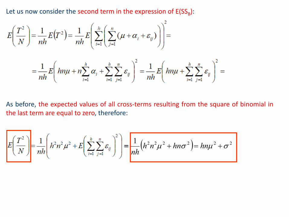
Let us now consider the second term in the expression of E(SSB):

As before, the expected values of all cross-terms resulting from the square of binomial inthe last term are equal to zero, therefore:

( ) 2222221 σµσµ +=+= hnhnnhnh

Combining the expressions evidenced by red rectangles in the last two slides, the followingexpression for E(SSB) is obtained:

( ) ( ) ( ) ∑∑∑

==

= +−=+−++=

−

=h

ii

h

ii

h

ii

B nhhnhnhnNTE

n

TESSE

1

22222

1

222

1

2

1 ασσµσαµ

Therefore:

( )

11

1

1)( 1

2

21

22

−+=

−

+−=

−=

∑∑==

h

n

h

nh

hSSEMSE

h

ii

h

ii

BB

ασ

ασ

22)( FB nMSE σσ +=

If σ2F is defined as:

The following expression is finally obtained:

11

2

2

−=

∑=

h

h

ii

F

ασ

If the Within-group mean square, MSW, is considered, the following equations can be written:

( )

−

−=

−= ∑∑ ∑

= = =

h

i

n

j

h

iiij

wW T

nXE

hNhNSSEMSE

1 1 1

22 11

Thus:

( ) ( )

++−++

−= ∑∑ ∑ ∑

= = = =

h

i

n

j

h

iij

n

jiijiW n

EhN

MSE1 1 1

2

1

2 )(11 εαµεαµ

Hence:

( ) 22

1

222

1

221 σσαµσαµ =

−−−++

−= ∑∑

==

hnNNnNhN

MSEh

ii

h

iiW

The results obtained so far can be summarized using the following table:

Source of variation SS df MS E(MS)

Betweengroup h-1 σ 2 + nσF

2

Withingroup

N-h σ 2

Total N-1NTX

h

i

n

jij

2

1 1

2 −∑∑= =

NT

n

Th

ii 2

1

2

−∑

= 1−=

hSSMS B

B

hNSSMS W

W −=∑∑

∑= =

=−h

i

n

j

h

ii

ij n

TX

1 1

1

2

2

If H1 is true (i.e., some, or all, αi ≠ 0) σF2 > 0 and MSB estimates σ 2 plus a positive

term that incorporates the variation due to the systematic difference in group means.

If H0 is true (i.e., all αi = 0) σF2 = 0, thus the between-group mean square MSB is an

unbiased estimator of σ 2, i.e., of the random error of measurement.

Interestingly, the within-group mean square MSW is an unbiased estimator of σ 2 regardlessof whether or not H0 is true, which is reasonable.

Under the assumption that each of the h groups can be modeled as a normal distribution, itcan be shown that:

is distributed as Fh-1,N-h

If the alternative hypothesis, H1, is true, the expected value of F0 numerator is higher thanthat of the denominator.

Consequently, H0 should be rejected if the realization of F0 is larger than the critical value.This implies the consideration of an upper-tail (one tail) critical region, i.e., theconsideration of a Fh-1, N-h,(1-α) as critical value.

W

B

MSMSF =0

0 1 2 3 40.0

0.2

0.4

0.6

0.8As an example, let us considerthe F4,30 distribution:

If α = 0.05, the critical valuecorresponds to 2.69.

Consequently, if F0 < 2.69, H0is accepted at a 5%significance level.

rejectionacceptance

Note that the same test can be made also using the P-Value, which corresponds to the areaunderlying the F curve, as calculated from the value assumed by F0 to infinity.

If P-value > α H0 is accepted, if P-value < α H0 is rejected.

The typical format of an ANOVA table provided by a statistical software is:

Source of variation

SS df MS F ratio P value Fcritical

Betweengroups

SSB h-1 MSB Tail area from F0

to infinityFh-1, N-h, (1-α )

Within groups SSW N-h MSW

Total SST N-1

W

B

MSMSF =0

Fixed versus Random Factors in the Analysis of Variance

In the preceding sections the standard analysis of variance (ANOVA) for a single-factorexperiment was discussed by assuming that the factor was a fixed factor. The term “fixedfactor” means that all the levels of the factor of interest were studied in the experiment.

Sometimes the levels of a factor are selected at random from a large (theoretically infinite)population of factor levels. This leads to a random-effects ANOVA model.

The model can be formally expressed as before:

However, the treatment effects, αi, are random variables, assumed to be normally andindependently distributed, with mean zero and variance σα

2.

The variance of an observation can be then expressed as:

Xij = µ + αi + εij

V(Xij) = V(µ + αi + εij) = V(αi) + V(εij) = σα2 + σ2

All of the computations in the random effect model are the same as in the fixed effectmodel, but since an entire population of treatments is studied, it does not make much senseto formulate hypotheses about the individual factor levels selected in the experiment.

Instead, the following hypotheses about the variance of the treatment effects are tested:

H0: σα2 = 0

H1: σα2 > 0

The test statistic for these hypotheses is the usual F-ratio: MSTreatments/MSError.

If the null hypothesis is not rejected there is no variability in the population of treatments,while if the null hypothesis is rejected there is a significant variability among the treatmentsin the entire population that was sampled.

Notice that the conclusions of ANOVA extend to the entire population of treatments.

The expected mean squares in the random model are different from their counterparts inthe fixed effects model. It can be shown that:

E(MSTreatments) = σ 2 + n σα2

E(MSError) = σ 2

Frequently, the goal of an experiment involving random factors is to estimate the variancecomponents.

A logical way to do this is to equate the expected values of the mean squares to theirobserved values and solve the resulting equations. This leads to:

)n

MSEMSE ErrorTreatments )((2 −=ασ

)(2ErrorMSE=σ

Examples of ANOVA applications

1) Tensile strength of paper

A manufacturer of paper used for making grocery bags is interested in improving thetensile strength of the product. Product engineers think that tensile strength is a functionof the hardwood concentration in the pulp and that the range of hardwood concentrationsof practical interest is between 5% and 20%.

A team of engineers responsible for the study decides to investigate four levels ofhardwood concentration: 5%, 10%, 15%, and 20%.They decide to make up six test specimens at each concentration level, using a pilot plant.All 24 specimens are tested on a laboratory tensile tester, in random order.

The data obtained from this experiment are shown in the following table:

This is an example of a completely randomized single-factor experiment with four levelsof the factor.

The role of randomization in this experiment is extremely important. By randomizing theorder of the 24 runs, the effect of any nuisance variable that may influence the observedtensile strength is approximately balanced out.

An example of nuisance variable could be a warm-up effect on the tensile strength testingmachine, leading to increasing values with operating time.

If all 24 runs were made in order of increasing hardwood concentration (that is, all six 5%concentration specimens were tested first, followed by all six 10% concentrationspecimens, etc.), then any observed differences in tensile strength could also be due tothe warm-up effect.

A Box-and-Whiskers plot can be adopted to represent data in a useful way.

The figure suggests that changing thehardwood concentration has an effect ontensile strength; specifically, higherhardwood concentrations produce higherobserved tensile strengths.

Furthermore, the distribution of tensilestrength at a particular hardwood level isgenerally not very asymmetric, and thevariability in tensile strength does not seemto change dramatically as the hardwoodconcentration changes.

A comparison between variances can bemade preliminarily to confirm thishypothesis.

The Minitab 18 software can be exploited to compare variances. They can be selected byaccessing the “Test for equal variances” option in the Stat > ANOVA> menu.

As an example, the Bartlett test, assuming a normal distribution for data in each group,indicates a p-value 0.769, thus suggesting that no significant difference is present betweenthe variances.The Levene’s test is consisting, giving a p-value 0.623.

The Minitab 18’s plot reporting confidence intervals for standard deviations of differentgroups, emphasizes the fact that an overlap occurs between them:

Manual ANOVA calculations

NTXSS

h

i

n

jijTotal

2

1 1

2 −= ∑∑= =

NT

n

TSS

h

ii

Treatments

21

2

−=∑

=

∑∑∑

= =

=−=h

i

n

j

h

ii

ijError n

TXSS

1 1

1

2

2

MSTreatments = 382.79/3 = 127.5097 MSError = 130.17/20 = 6.508

F0 = 127.597/6.508 = 19.61

Since the critical value is F0.99, 3.20 = 4.94, H0 should be rejected, thus the sample means differsignificantly. This can be inferred also from the P-value, which is 3.59 × 10-6 << 0.01.

ANOVA calculations with the Minitab 18 software

In the worksheet different factors(treatments) are represented by differentcolumns, whereas levels (replicates) arerepresented by different rows.

Different options (in the present casevariances are assumed to be equal, basedon the comparison of variances) andgraphical representations of results canbe selected.

2) Stability of a fluorescent reagent stored under different conditions

Table of data:

Mean squares can be calculated according to the first definition:

MSB = 62

MSW = 3

Since F0 = 62/3 = 20.7 and the critical value is 4.066 (α = 0.05), H0 should be rejected, thusthe sample means differ significantly.

Minitab 18 output

Note that the P value in the ANOVA table, rounded off to the third decimal place, is 0.

3) Example of ANOVA with a random-effect factor: purity testing of a barrel of sodiumchloride.

The following values were obtained after replicating four times the purity testing on fivesamples of sodium chloride taken from different parts of a barrel, chosen at random:

In this case two possible sources of variation can be hypothesized for the observed purity:

1) random error in the measurement of purity, given by the measurement variance σ2

2) variations in the sodium chloride purity at different points in the barrel, accounted forby sampling variance, corresponding to σα

2 defined before.

These are the results obtained from ANOVA calculations:

As apparent, since the realization of the F statistic, 30, is much higher than the criticalvalue (3.056), a significant difference exists between the purity of the different samples.

It is worth recalling that in this case the expected value for the between-sample-meansquare is given by:

Consequently, considering that σ2 corresponds to MSw, the following calculation can bemade to obtain an estimate of the sampling variance:

σα2 = (E(MSB) – σ2)/n = (1.96 - 0.0653)/4 = 0.47

𝐸𝐸(𝑀𝑀𝑆𝑆𝐵𝐵) = 𝜎𝜎2 + 𝑛𝑛𝜎𝜎𝑎𝑎2

4) Example of ANOVA with a complete evaluation of assumptions

Let us reconsider the set of 65 (5 replicates obtained by each of 13 groups) enthalpyvariations (kJ/mol) values measured for the neutralization of NaOH with HCl:

Group x1 x2 x3 x4 x5 x s2

1 56.9 59.2 56.3 58.0 56.9 57.46 1.32

2 53.8 55.4 58.0 59.6 55.5 56.46 5.34

3 58.4 55.0 55.7 56.6 57.2 56.58 1.74

4 58.0 56.4 57.6 57.5 55.0 56.90 1.48

5 57.7 58.5 58.9 57.8 57.4 58.06 0.38

6 54.8 56.4 55.2 60.3 57.1 56.76 4.76

7 57.1 60.4 58.9 55.5 54.7 57.32 5.55

8 58.6 57.8 58.0 55.5 55.6 57.10 2.09

9 58.9 59.8 60.0 57.1 56.4 58.44 2.61

10 59.5 57.7 60.0 57.6 56.8 58.32 1.86

11 57.2 58.2 57.4 55.7 59.1 57.52 1.60

12 55.4 56.1 57.7 56.9 59.2 57.06 2.17

13 55.1 56.8 55.7 61.6 58.3 57.50 6.74

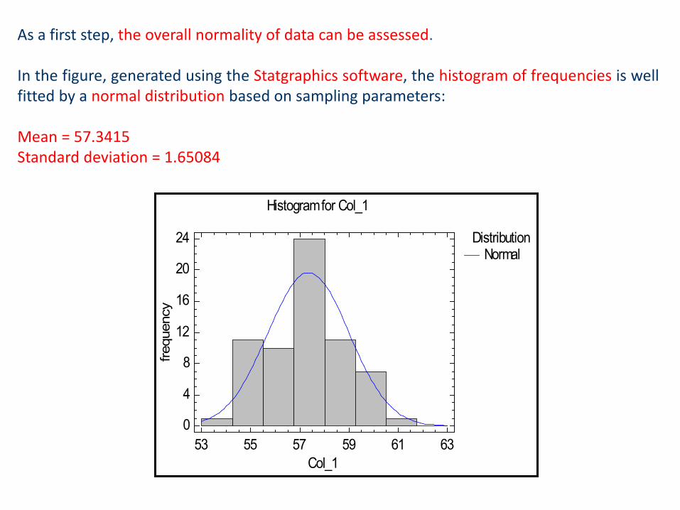
As a first step, the overall normality of data can be assessed.

In the figure, generated using the Statgraphics software, the histogram of frequencies is wellfitted by a normal distribution based on sampling parameters:

Mean = 57.3415Standard deviation = 1.65084

Histogram for Col_1

53 55 57 59 61 63Col_1

0

4

8

12

16

20

24

frequ

ency

DistributionNormal

The test for normality can be also performed using Minitab 18 , by accessing the NormalityTest… option in the Stat > Basic Statistics menu. The Kolmogorov-Smirnov test is available,among others.

If dots are closed to the red line, as in this case, data are likely to be distributed according toa Gaussian function at a 5% significance. Indeed, the P-value in this case is greater than0.150.

In the case of Minitab 18 theKolmogorov-Smirnov (KS) plot islinearized by using anappropriate vertical scale.

Dots correspond to steps in thetypical KS plots, whereas the redline correspond to the sigmoidalcurve for the theoreticalcumulative distribution function.

The ANOVA table generated by the Statgraphics software shows a relatively low value forthe F-Ratio (the name used for F0 in the program), with a p-value of 0.7669:

As a consequence, no significant difference can be inferred between the 13 groups of datain terms of mean values.

As for variances, the Levene’s test provides a p-value 0.769937, thus indicating thatvariances related to the 13 groups of data are not significant different.