Embed Size (px)
Citation preview
ANALYSIS OF VARIANCE (ANOVA)
Analysis of variance (abbreviated as ANOVA) is an extremely useful technique concerning researches
in the fields of economics, biology, education, psychology, sociology, business/industry and in researches
of several other disciplines. This technique is used when multiple sample cases are involved. As
stated earlier, the significance of the difference between the means of two samples can be judged
through either z-test or the t-test, but the difficulty arises when we happen to examine the significance
of the difference amongst more than two sample means at the same time. The ANOVA technique
enables us to perform this simultaneous test and as such is considered to be an important tool of
analysis in the hands of a researcher. Using this technique, one can draw inferences about whether
the samples have been drawn from populations having the same mean.
The ANOVA technique is important in the context of all those situations where we want to
compare more than two populations such as in comparing the yield of crop from several varieties of
seeds, the gasoline mileage of four automobiles, the smoking habits of five groups of university
students and so on. In such circumstances one generally does not want to consider all possible
combinations of two populations at a time for that would require a great number of tests before we
would be able to arrive at a decision. This would also consume lot of time and money, and even then
certain relationships may be left unidentified (particularly the interaction effects). Therefore, one
quite often utilizes the ANOVA technique and through it investigates the differences among the
means of all the populations simultaneously.
WHAT IS ANOVA?
Professor R.A. Fisher was the first man to use the term ‘Variance’* and, in fact, it was he who
developed a very elaborate theory concerning ANOVA, explaining its usefulness in practical field.
* Variance is an important statistical measure and is described as the mean of the squares of deviations taken from the mean of the given series of data. It is a frequently used measure of variation. Its squareroot is known as standard
deviation,
i.e., Standard deviation = Variance.
Analysis of Variance and Co-variance 257
Later on Professor Snedecor and many others contributed to the development of this technique.
ANOVA is essentially a procedure for testing the difference among different groups of data for
homogeneity. “The essence of ANOVA is that the total amount of variation in a set of data is broken
down into two types, that amount which can be attributed to chance and that amount which can be
attributed to specified causes.”1 There may be variation between samples and also within sample
items. ANOVA consists in splitting the variance for analytical purposes. Hence, it is a method of
analysing the variance to which a response is subject into its various components corresponding to
various sources of variation. Through this technique one can explain whether various varieties of
seeds or fertilizers or soils differ significantly so that a policy decision could be taken accordingly,
concerning a particular variety in the context of agriculture researches. Similarly, the differences in
various types of feed prepared for a particular class of animal or various types of drugs manufactured
for curing a specific disease may be studied and judged to be significant or not through the application
of ANOVA technique. Likewise, a manager of a big concern can analyse the performance of
various salesmen of his concern in order to know whether their performances differ significantly.
Thus, through ANOVA technique one can, in general, investigate any number of factors which
are hypothesized or said to influence the dependent variable. One may as well investigate the
differences amongst various categories within each of these factors which may have a large number
of possible values. If we take only one factor and investigate the differences amongst its various
categories having numerous possible values, we are said to use one-way ANOVA and in case we
investigate two factors at the same time, then we use two-way ANOVA. In a two or more way
ANOVA, the interaction (i.e., inter-relation between two independent variables/factors), if any, between
two independent variables affecting a dependent variable can as well be studied for better decisions.
THE BASIC PRINCIPLE OF ANOVA
The basic principle of ANOVA is to test for differences among the means of the populations by
examining the amount of variation within each of these samples, relative to the amount of variation
between the samples. In terms of variation within the given population, it is assumed that the values
of (Xij) differ from the mean of this population only because of random effects i.e., there are influences
on (Xij) which are unexplainable, whereas in examining differences between populations we assume
that the difference between the mean of the jth population and the grand mean is attributable to what
is called a ‘specific factor’ or what is technically described as treatment effect. Thus while using
ANOVA, we assume that each of the samples is drawn from a normal population and that each of
these populations has the same variance. We also assume that all factors other than the one or more
being tested are effectively controlled. This, in other words, means that we assume the absence of
many factors that might affect our conclusions concerning the factor(s) to be studied.
In short, we have to make two estimates of population variance viz., one based on between
samples variance and the other based on within samples variance. Then the said two estimates of
population variance are compared with F-test, wherein we work out.
F Estimate of population variance based on between samples variance
Estimate of population variance based on within samples variance
1 Donald L. Harnett and James L. Murphy, Introductory Statistical Analysis, p. 376.
1
1 i2 2 ki k
258 Research Methodology
This value of F is to be compared to the F-limit for given degrees of freedom. If the F value we
work out is equal or exceeds* the F-limit value (to be seen from F tables No. 4(a) and 4(b) given in
appendix), we may say that there are significant differences between the sample means.
ANOVA TECHNIQUE
One-way (or single factor) ANOVA: Under the one-way ANOVA, we consider only one factor
and then observe that the reason for said factor to be important is that several possible types of
samples can occur within that factor. We then determine if there are differences within that factor.
The technique involves the following steps:
(i) Obtain the mean of each sample i.e., obtain
X1, X 2, X 3 , ..., Xk
when there are k samples.
(ii) Work out the mean of the sample means as follows:
X X1 X 2 X 3 ... Xk
No. of samples (k )
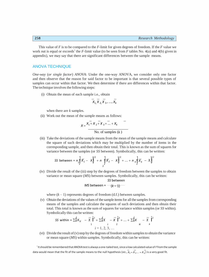
(iii) Take the deviations of the sample means from the mean of the sample means and calculate
the square of such deviations which may be multiplied by the number of items in the
corresponding sample, and then obtain their total. This is known as the sum of squares for
variance between the samples (or SS between). Symbolically, this can be written:
SS between = n Jy X1 X yJ2
n Jy X 2 X yJ2
... n k Jy X k X yJ
2
(iv) Divide the result of the (iii) step by the degrees of freedom between the samples to obtain
variance or mean square (MS) between samples. Symbolically, this can be written:
MS between =
SS between
(k – 1)
where (k – 1) represents degrees of freedom (d.f.) between samples.
(v) Obtain the deviations of the values of the sample items for all the samples from corresponding
means of the samples and calculate the squares of such deviations and then obtain their
total. This total is known as the sum of squares for variance within samples (or SS within).
Symbolically this can be written:
SS within = d X1i X i2 dX X i2
... dX X i2
i = 1, 2, 3, …
(vi) Divide the result of (v) step by the degrees of freedom within samples to obtain the variance
or mean square (MS) within samples. Symbolically, this can be written:
* It should be remembered that ANOVA test is always a one-tailed test, since a low calculated value of F from the sample
data would mean that the fit of the sample means to the null hypothesis (viz., X1 X 2 ... X k ) is a very good fit.
2
Analysis of Variance and Co-variance 259
MS within = SS within
(n – k )
where (n – k) represents degrees of freedom within samples,
n = total number of items in all the samples i.e., n1 + n
2 + … + n
k
k = number of samples.
(vii) For a check, the sum of squares of deviations for total variance can also be worked out by
adding the squares of deviations when the deviations for the individual items in all the
samples have been taken from the mean of the sample means. Symbolically, this can be
written:
SS for total variance = Jy X ij X yJ2
i = 1, 2, 3, …
j = 1, 2, 3, …
This total should be equal to the total of the result of the (iii) and (v) steps explained above
i.e.,
SS for total variance = SS between + SS within.
The degrees of freedom for total variance will be equal to the number of items in all
samples minus one i.e., (n – 1). The degrees of freedom for between and within must add
up to the degrees of freedom for total variance i.e.,
(n – 1) = (k – 1) + (n – k)
This fact explains the additive property of the ANOVA technique.
(viii) Finally, F-ratio may be worked out as under:
F -ratio =
MS between
MS within
This ratio is used to judge whether the difference among several sample means is significant
or is just a matter of sampling fluctuations. For this purpose we look into the table*, giving
the values of F for given degrees of freedom at different levels of significance. If the
worked out value of F, as stated above, is less than the table value of F, the difference is
taken as insignificant i.e., due to chance and the null-hypothesis of no difference between
sample means stands. In case the calculated value of F happens to be either equal or more
than its table value, the difference is considered as significant (which means the samples
could not have come from the same universe) and accordingly the conclusion may be
drawn. The higher the calculated value of F is above the table value, the more definite and
sure one can be about his conclusions.
SETTING UP ANALYSIS OF VARIANCE TABLE
For the sake of convenience the information obtained through various steps stated above can be put
as under:
* An extract of table giving F-values has been given in Appendix at the end of the book in Tables 4 (a) and 4 (b).
260 Research Methodology
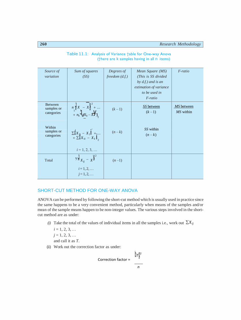
Table 11.1: Analysis of Variance †able for One-way Anova
(†here are k samples having in all n items)
Source of
variation
Sum of squares
(SS)
Degrees of
freedom (d.f.)
Mean Square (MS)
(This is SS divided
by d.f.) and is an
estimation of variance
to be used in
F-ratio
F-ratio
Between n Jy X X yJ
2
... 1 1
nk Jy Xk X yJ 2
2
d X1i X1 i ...
d X ki X k i 2
i = 1, 2, 3, …
(k – 1)
(n – k)
SS between
(k – 1)
SS within
(n – k )
MS between
MS within samples or
categories
Within samples or
categories
Total Jy yJ
2
X ij X
i = 1, 2, …
j = 1, 2, …
(n –1)
SHORT-CUT METHOD FOR ONE-WAY ANOVA
ANOVA can be performed by following the short-cut method which is usually used in practice since
the same happens to be a very convenient method, particularly when means of the samples and/or
mean of the sample means happen to be non-integer values. The various steps involved in the short-
cut method are as under:
(i) Take the total of the values of individual items in all the samples i.e., work out Xij
i = 1, 2, 3, …
j = 1, 2, 3, …
and call it as T.
(ii) Work out the correction factor as under:
Correction factor = bT g2
n
ij
j
j
ij
Analysis of Variance and Co-variance 261
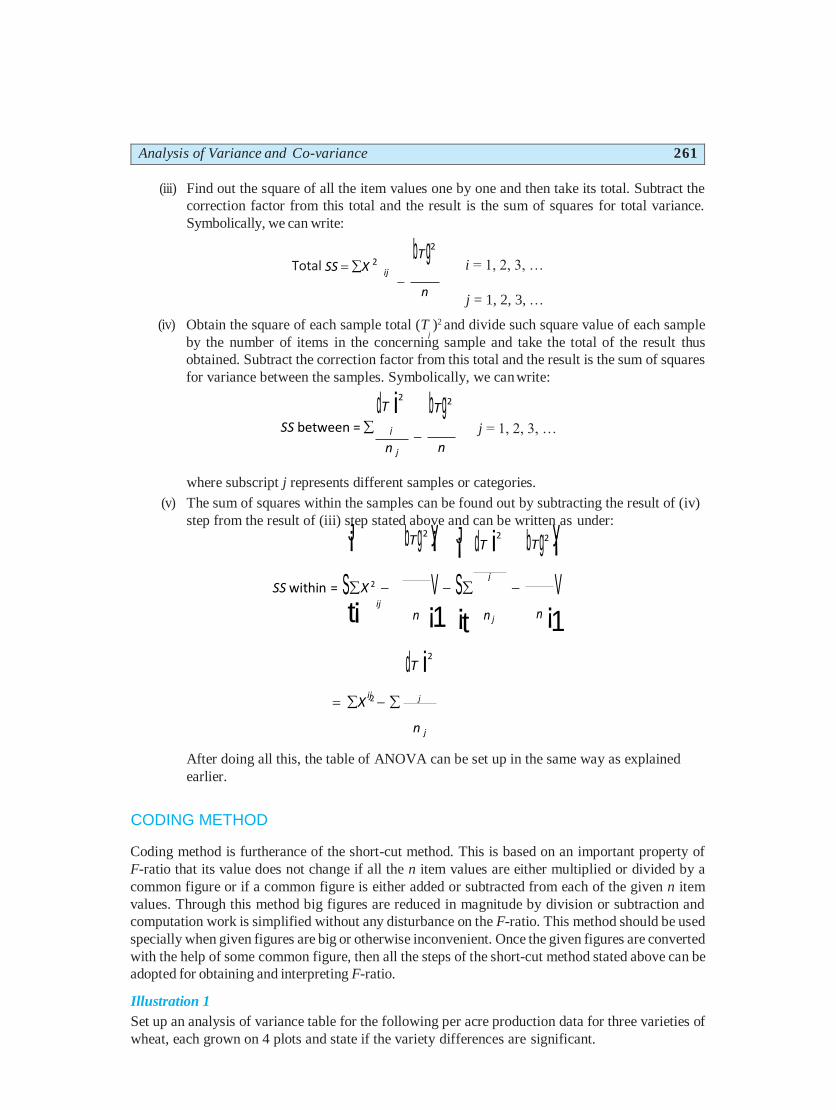
(iii) Find out the square of all the item values one by one and then take its total. Subtract the
correction factor from this total and the result is the sum of squares for total variance.
Symbolically, we can write:
Total SS X 2
bT g2
n
i = 1, 2, 3, …
j = 1, 2, 3, …
(iv) Obtain the square of each sample total (T )2 and divide such square value of each sample
by the number of items in the concerning sample and take the total of the result thus
obtained. Subtract the correction factor from this total and the result is the sum of squares
for variance between the samples. Symbolically, we can write:
SS between =
dT i2
n j
bTg2
n
j = 1, 2, 3, …
where subscript j represents different samples or categories.
(v) The sum of squares within the samples can be found out by subtracting the result of (iv)
step from the result of (iii) step stated above and can be written as under:
¡J bT g2 y¡
¡J dT i2
bT g2 y¡
SS within = SX 2 V S V t¡
ij
n ¡1 ¡t n j n ¡1
dT i2
X 2 j
n j
After doing all this, the table of ANOVA can be set up in the same way as explained
earlier.
CODING METHOD
Coding method is furtherance of the short-cut method. This is based on an important property of
F-ratio that its value does not change if all the n item values are either multiplied or divided by a
common figure or if a common figure is either added or subtracted from each of the given n item
values. Through this method big figures are reduced in magnitude by division or subtraction and
computation work is simplified without any disturbance on the F-ratio. This method should be used
specially when given figures are big or otherwise inconvenient. Once the given figures are converted
with the help of some common figure, then all the steps of the short-cut method stated above can be
adopted for obtaining and interpreting F-ratio.
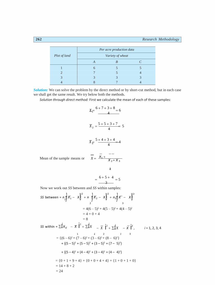
Illustration 1
Set up an analysis of variance table for the following per acre production data for three varieties of
wheat, each grown on 4 plots and state if the variety differences are significant.
j
1
1 i2 2 i3 3
3
262 Research Methodology
Plot of land
Per acre production data
Variety of wheat
A B C
1 6 5 5
2 7 5 4
3 3 3 3
4 8 7 4
Solution: We can solve the problem by the direct method or by short-cut method, but in each case
we shall get the same result. We try below both the methods.
Solution through direct method: First we calculate the mean of each of these samples:
X 6 7 3 8
6
1 4
X 5 5 3 7
5
2 4
X 5 4 3 4
4
3 4
Mean of the sample means or X
X1
X 2 X 3
k
6 5 4
5
3
Now we work out SS between and SS within samples:
SS between = n Jy X1 X yJ2
n Jy X 2 X yJ2
n3 Jy X X yJ
2
= 4(6 – 5)2 + 4(5 – 5)2 + 4(4 – 5)2
= 4 + 0 + 4
= 8
SS within = d X1i X i2 dX X i2
d X X i2 , i = 1, 2, 3, 4
= {(6 – 6)2 + (7 – 6)2 + (3 – 6)2 + (8 – 6)2}
+ {(5 – 5)2 + (5 – 5)2 + (3 – 5)2 + (7 – 5)2}
+ {(5 – 4)2 + (4 – 4)2 + (3 – 4)2 + (4 – 4)2}
= {0 + 1 + 9 + 4} + {0 + 0 + 4 + 4} + {1 + 0 + 1 + 0}
= 14 + 8 + 2
= 24
2
ij
Analysis of Variance and Co-variance 263
SS for total variance = Jy X ij X yJ2
i = 1, 2, 3…
j = 1, 2, 3…
= (6 – 5)2 + (7 – 5)2 + (3 – 5)2 + (8 – 5)2
+ (5 – 5)2 + (5 – 5)2 + (3 – 5)2
+ (7 – 5)2 + (5 – 5)2 + (4 – 5)2
+ (3 – 5)2 + (4 – 5)2
= 1 + 4 + 4 + 9 + 0 + 0 + 4 + 4 + 0 + 1 + 4 + 1
= 32
Alternatively, it (SS for total variance) can also be worked out thus:
SS for total = SS between + SS within
= 8 + 24
= 32
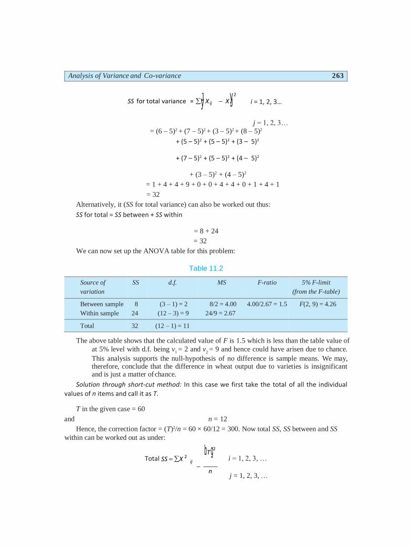
We can now set up the ANOVA table for this problem:
Table 11.2
Source of
variation
SS d.f. MS F-ratio 5% F-limit
(from the F-table)
Between sample 8 (3 – 1) = 2 8/2 = 4.00 4.00/2.67 = 1.5 F(2, 9) = 4.26
Within sample 24 (12 – 3) = 9 24/9 = 2.67
Total 32 (12 – 1) = 11
The above table shows that the calculated value of F is 1.5 which is less than the table value of
at 5% level with d.f. being v1 = 2 and v
2 = 9 and hence could have arisen due to chance.
This analysis supports the null-hypothesis of no difference is sample means. We may, therefore, conclude that the difference in wheat output due to varieties is insignificant and is just a matter of chance.
Solution through short-cut method: In this case we first take the total of all the individual
values of n items and call it as T.
T in the given case = 60
and n = 12
Hence, the correction factor = (T)2/n = 60 × 60/12 = 300. Now total SS, SS between and SS
within can be worked out as under:
Total SS X 2
bT g2
n
i = 1, 2, 3, …
j = 1, 2, 3, …
j
ij dT i
264 Research Methodology
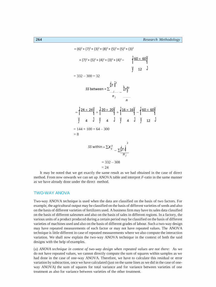
= (6)2 + (7)2 + (3)2 + (8)2 + (5)2 + (5)2 + (3)2
+ (7)2 + (5)2 + (4)2 + (3)2 + (4)2 – J¡ 60 60y¡
= 332 – 300 = 32
SS between =
dT i2
n j
y
bT g2
n
12 J
J¡ 24 24y¡
J¡ 20 20y¡ J¡16 16y¡
J¡ 60 60y¡
y 4 J y 4 J y 4 J y 12 J = 144 + 100 + 64 – 300
= 8
SS within X 2
2
j n j
= 332 – 308
= 24
It may be noted that we get exactly the same result as we had obtained in the case of direct
method. From now onwards we can set up ANOVA table and interpret F-ratio in the same manner
as we have already done under the direct method.
TWO-WAY ANOVA
Two-way ANOVA technique is used when the data are classified on the basis of two factors. For
example, the agricultural output may be classified on the basis of different varieties of seeds and also
on the basis of different varieties of fertilizers used. A business firm may have its sales data classified
on the basis of different salesmen and also on the basis of sales in different regions. In a factory, the
various units of a product produced during a certain period may be classified on the basis of different
varieties of machines used and also on the basis of different grades of labour. Such a two-way design
may have repeated measurements of each factor or may not have repeated values. The ANOVA
technique is little different in case of repeated measurements where we also compute the interaction
variation. We shall now explain the two-way ANOVA technique in the context of both the said
designs with the help of examples.
(a) ANOVA technique in context of two-way design when repeated values are not there: As we
do not have repeated values, we cannot directly compute the sum of squares within samples as we
had done in the case of one-way ANOVA. Therefore, we have to calculate this residual or error
variation by subtraction, once we have calculated (just on the same lines as we did in the case of one-
way ANOVA) the sum of squares for total variance and for variance between varieties of one
treatment as also for variance between varieties of the other treatment.
ij
Analysis of Variance and Co-variance 265
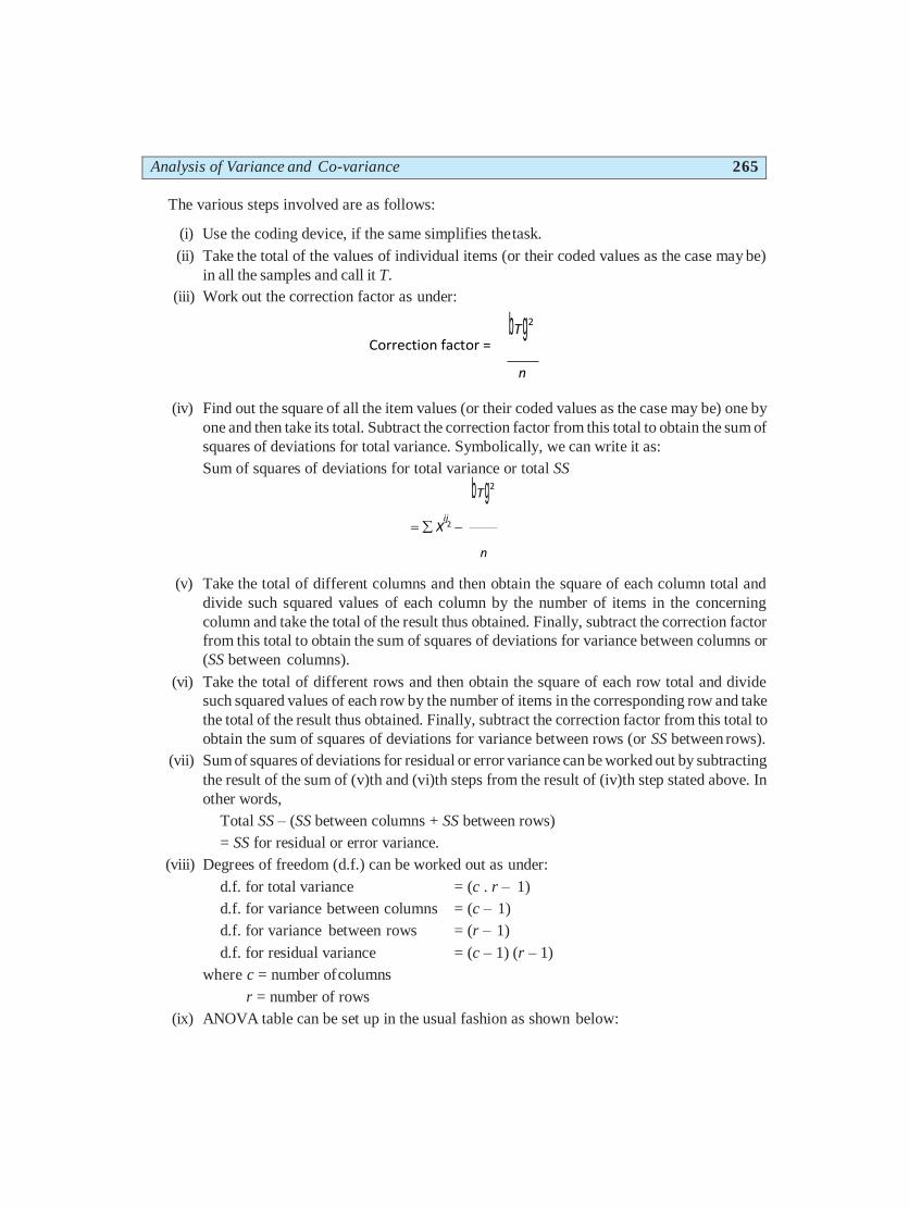
The various steps involved are as follows:
(i) Use the coding device, if the same simplifies the task.
(ii) Take the total of the values of individual items (or their coded values as the case may be)
in all the samples and call it T.
(iii) Work out the correction factor as under:
Correction factor = bT g2
n
(iv) Find out the square of all the item values (or their coded values as the case may be) one by
one and then take its total. Subtract the correction factor from this total to obtain the sum of
squares of deviations for total variance. Symbolically, we can write it as:
Sum of squares of deviations for total variance or total SS
bT g2
X 2
n
(v) Take the total of different columns and then obtain the square of each column total and
divide such squared values of each column by the number of items in the concerning
column and take the total of the result thus obtained. Finally, subtract the correction factor
from this total to obtain the sum of squares of deviations for variance between columns or
(SS between columns).
(vi) Take the total of different rows and then obtain the square of each row total and divide
such squared values of each row by the number of items in the corresponding row and take
the total of the result thus obtained. Finally, subtract the correction factor from this total to
obtain the sum of squares of deviations for variance between rows (or SS between rows).
(vii) Sum of squares of deviations for residual or error variance can be worked out by subtracting
the result of the sum of (v)th and (vi)th steps from the result of (iv)th step stated above. In
other words,
Total SS – (SS between columns + SS between rows)
= SS for residual or error variance.
(viii) Degrees of freedom (d.f.) can be worked out as under:
d.f. for total variance = (c . r – 1)
d.f. for variance between columns = (c – 1)
d.f. for variance between rows = (r – 1)
d.f. for residual variance = (c – 1) (r – 1)
where c = number of columns
r = number of rows
(ix) ANOVA table can be set up in the usual fashion as shown below:
266 Research Methodology
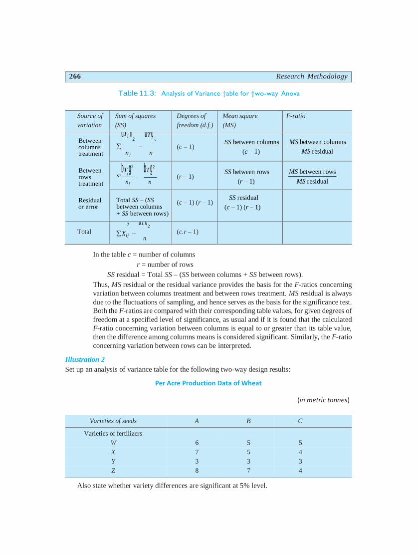
Table 11.3: Analysis of Variance †able for †wo-way Anova
Source of
variation
Sum of squares
(SS)
Degrees of
freedom (d.f.)
Mean square
(MS)
F-ratio
Between columns treatment
Between rows treatment
Residual or error
dTj i bTg 2 2
n j n
(c – 1)
SS between columns
(c – 1)
MS between columns
MS residual
bT g2 bT g2
i
ni n
(r – 1)
SS between rows
(r – 1)
MS between rows
MS residual
Total SS – (SS between columns + SS between rows)
(c – 1) (r – 1) SS residual
(c – 1) (r – 1)
Total
2 bT g 2
Xij n
(c.r – 1)
In the table c = number of columns
r = number of rows
SS residual = Total SS – (SS between columns + SS between rows).
Thus, MS residual or the residual variance provides the basis for the F-ratios concerning
variation between columns treatment and between rows treatment. MS residual is always
due to the fluctuations of sampling, and hence serves as the basis for the significance test.
Both the F-ratios are compared with their corresponding table values, for given degrees of
freedom at a specified level of significance, as usual and if it is found that the calculated
F-ratio concerning variation between columns is equal to or greater than its table value,
then the difference among columns means is considered significant. Similarly, the F-ratio
concerning variation between rows can be interpreted.
Illustration 2
Set up an analysis of variance table for the following two-way design results:
Per Acre Production Data of Wheat
(in metric tonnes)
Varieties of seeds A B C
Varieties of fertilizers
W 6 5 5
X 7 5 4
Y 3 3 3
Z 8 7 4
Also state whether variety differences are significant at 5% level.
Analysis of Variance and Co-variance 267
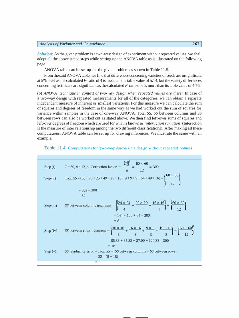
Solution: As the given problem is a two-way design of experiment without repeated values, we shall
adopt all the above stated steps while setting up the ANOVA table as is illustrated on the following
page.
ANOVA table can be set up for the given problem as shown in Table 11.5.
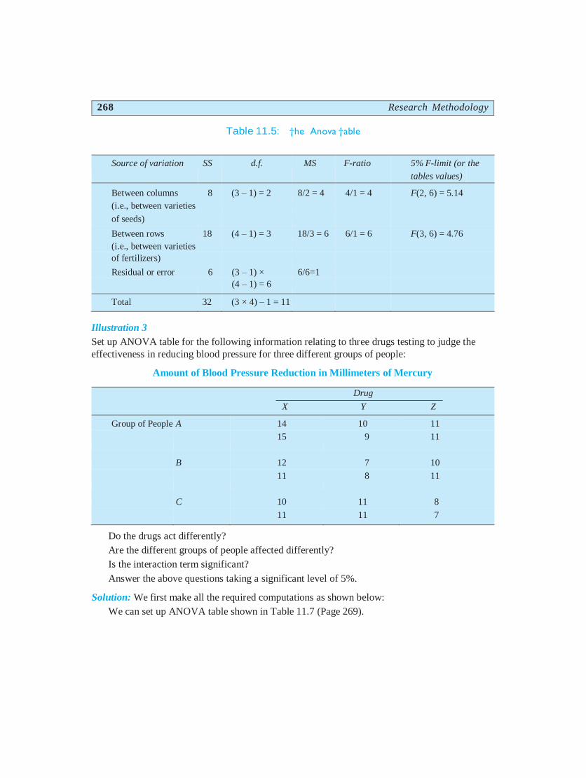
From the said ANOVA table, we find that differences concerning varieties of seeds are insignificant
at 5% level as the calculated F-ratio of 4 is less than the table value of 5.14, but the variety differences
concerning fertilizers are significant as the calculated F-ratio of 6 is more than its table value of 4.76.
(b) ANOVA technique in context of two-way design when repeated values are there: In case of
a two-way design with repeated measurements for all of the categories, we can obtain a separate
independent measure of inherent or smallest variations. For this measure we can calculate the sum
of squares and degrees of freedom in the same way as we had worked out the sum of squares for
variance within samples in the case of one-way ANOVA. Total SS, SS between columns and SS
between rows can also be worked out as stated above. We then find left-over sums of squares and
left-over degrees of freedom which are used for what is known as ‘interaction variation’ (Interaction
is the measure of inter relationship among the two different classifications). After making all these
computations, ANOVA table can be set up for drawing inferences. We illustrate the same with an
example.
Table 11.4: Computations for †wo-way Anova (in a design without repeated values)
bT g2 60 60
Step (i) T = 60, n = 12, Correction factor = 300 n 12
Step (ii) Total SS = (36 + 25 + 25 + 49 + 25 + 16 + 9 + 9 + 9 + 64 + 49 + 16) – ¡J 60 60¡y y 12 J
= 332 – 300
= 32
Step (iii) SS between columns treatment µ¡µ24 24
20 20
16 16 y¡J
µ¡µ60 60 y¡J 4 4 4 12
= 144 + 100 + 64 – 300
= 8
Step (iv) SS between rows treatment µ¡µ16 16
16 16
9 9
19 19 y¡J
µ¡µ60 60 y¡J 3 3 3 3 12
= 85.33 + 85.33 + 27.00 + 120.33 – 300
= 18
Step (v) SS residual or error = Total SS – (SS between columns + SS between rows)
= 32 – (8 + 18)
= 6
268 Research Methodology
Table 11.5: †he Anova †able
Source of variation SS d.f. MS F-ratio 5% F-limit (or
tables values)
the
Between columns 8 (3 – 1) = 2 8/2 = 4 4/1 = 4 F(2, 6) = 5.14
(i.e., between varieties
of seeds)
Between rows 18 (4 – 1) = 3 18/3 = 6 6/1 = 6 F(3, 6) = 4.76
(i.e., between varieties
of fertilizers)
Residual or error 6 (3 – 1) × 6/6=1
(4 – 1) = 6
Total 32 (3 × 4) – 1 = 11
Illustration 3
Set up ANOVA table for the following information relating to three drugs testing to judge the
effectiveness in reducing blood pressure for three different groups of people:
Amount of Blood Pressure Reduction in Millimeters of Mercury
Drug
X Y Z
Group of People A 14 10 11
15 9 11
B 12 7 10
11 8 11
C 10 11 8
11 11 7
Do the drugs act differently?
Are the different groups of people affected differently?
Is the interaction term significant?
Answer the above questions taking a significant level of 5%.
Solution: We first make all the required computations as shown below:
We can set up ANOVA table shown in Table 11.7 (Page 269).
Analysis of Variance and Co-variance 269
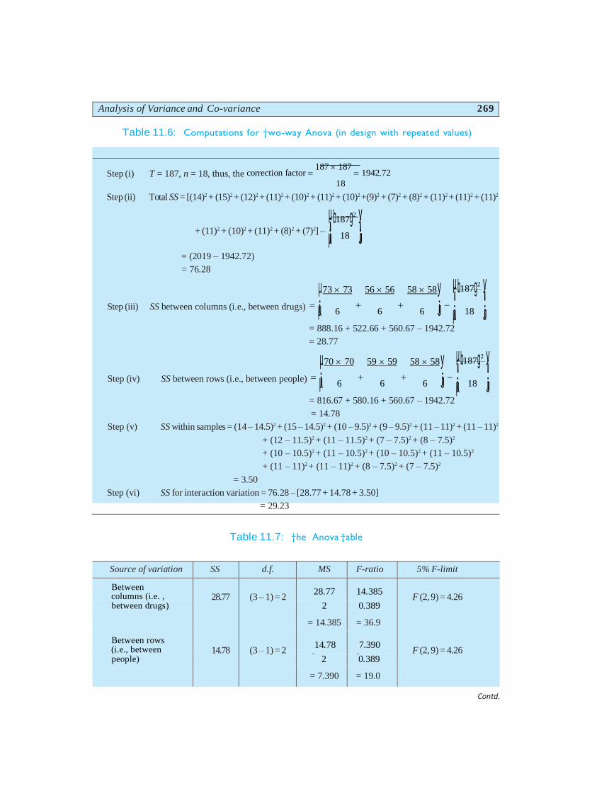
Table 11.6: Computations for †wo-way Anova (in design with repeated values)
Step (i) T = 187, n = 18, thus, the correction factor 187 187
1942.72 18
Step (ii) Total SS = [(14)2 + (15)2 + (12)2 + (11)2 + (10)2 + (11)2 + (10)2 +(9)2 + (7)2 + (8)2 + (11)2 + (11)2 + (11)2
µ¡b187g2 y¡
+ (11)2 + (10)2 + (11)2 + (8)2 + (7)2] – ¡µ 18 ¡J
= (2019 – 1942.72)
= 76.28
µ73 73 56 56 58 58y µ¡b187g2 y¡ Step (iii) SS between columns (i.e., between drugs) ¡µ 6
6
6 ¡J ¡µ 18 ¡J
= 888.16 + 522.66 + 560.67 – 1942.72
= 28.77
µ70 70 59 59 58 58 y µ¡b187g2 y¡ Step (iv) SS between rows (i.e., between people) ¡µ 6
6
6 ¡J ¡µ 18 ¡J
= 816.67 + 580.16 + 560.67 – 1942.72
= 14.78
Step (v) SS within samples = (14 – 14.5)2 + (15 – 14.5)2 + (10 – 9.5)2 + (9 – 9.5)2 + (11 – 11)2 + (11 – 11)2
+ (12 – 11.5)2 + (11 – 11.5)2 + (7 – 7.5)2 + (8 – 7.5)2
+ (10 – 10.5)2 + (11 – 10.5)2 + (10 – 10.5)2 + (11 – 10.5)2
+ (11 – 11)2 + (11 – 11)2 + (8 – 7.5)2 + (7 – 7.5)2
= 3.50
Step (vi) SS for interaction variation = 76.28 – [28.77 + 14.78 + 3.50]
= 29.23
Table 11.7: †he Anova †able
Source of variation SS d.f. MS F-ratio 5% F-limit
Between columns (i.e. ,
28.77
14.78
(3 – 1) = 2
(3 – 1) = 2
28.77 14.385
F (2, 9) = 4.26
F (2, 9) = 4.26
between drugs) 2 0.389
= 14.385 = 36.9
Between rows (i.e., between
14.78 7.390
people) 2 0.389
= 7.390 = 19.0
Contd.
270 Research Methodology
Source of variation SS d.f. MS F-ratio 5% F-limit
Interaction 29.23* 4*
29.23
4
7.308
0.389 F (4, 9) = 3.63
Within samples (Error)
3.50
(18 – 9) = 9
3.50
9
= 0.389
Total 76.28 (18 – 1) = 17
* These figures are left-over figures and have been obtained by subtracting from the column total the total of all
other value in the said column. Thus, interaction SS = (76.28) – (28.77 + 14.78 + 3.50) = 29.23 and interaction degrees of freedom
= (17) – (2 + 2 + 9) = 4.
The above table shows that all the three F-ratios are significant of 5% level which means that
the drugs act differently, different groups of people are affected differently and the interaction term
is significant. In fact, if the interaction term happens to be significant, it is pointless to talk about the
differences between various treatments i.e., differences between drugs or differences between
groups of people in the given case.
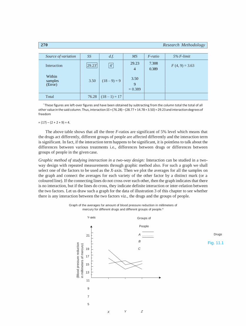
Graphic method of studying interaction in a two-way design: Interaction can be studied in a two-
way design with repeated measurements through graphic method also. For such a graph we shall
select one of the factors to be used as the X-axis. Then we plot the averages for all the samples on
the graph and connect the averages for each variety of the other factor by a distinct mark (or a
coloured line). If the connecting lines do not cross over each other, then the graph indicates that there
is no interaction, but if the lines do cross, they indicate definite interaction or inter-relation between
the two factors. Let us draw such a graph for the data of illustration 3 of this chapter to see whether
there is any interaction between the two factors viz., the drugs and the groups of people.
Graph of the averages for amount of blood pressure reduction in millimeters of
mercury for different drugs and different groups of people.*
Y-axis Groups of
People
21 A
B
19 C
17
15
13
11
9
7
5
X Y Z
Drugs
Fig. 11.1
(Blo
od
pre
ssure
re
ductio
n
in m
illim
ete
rs o
f m
erc
ury
)

X-axis
* Alternatively, the graph can be drawn by taking different group of people on X-axis and drawing lines for various drugs
through the averages.
Analysis of Variance and Co-variance 271
The graph indicates that there is a significant interaction because the different connecting lines
for groups of people do cross over each other. We find that A and B are affected very similarly, but
C is affected differently. The highest reduction in blood pressure in case of C is with drug Y and the
lowest reduction is with drug Z, whereas the highest reduction in blood pressure in case of A and B
is with drug X and the lowest reduction is with drug Y. Thus, there is definite inter-relation between
the drugs and the groups of people and one cannot make any strong statements about drugs unless he
also qualifies his conclusions by stating which group of people he is dealing with. In such a situation,
performing F-tests is meaningless. But if the lines do not cross over each other (and remain more or
less identical), then there is no interaction or the interaction is not considered a significantly large
value, in which case the researcher should proceed to test the main effects, drugs and people in the
given case, as stated earlier.
ANOVA IN LATIN-SQUARE DESIGN
Latin-square design is an experimental design used frequently in agricultural research. In such a
design the treatments are so allocated among the plots that no treatment occurs, more than once in
any one row or any one column. The ANOVA technique in case of Latin-square design remains
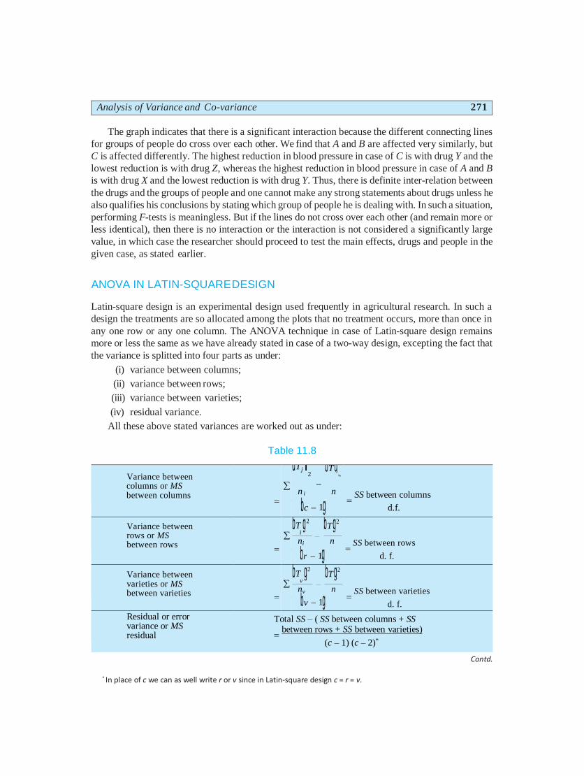
more or less the same as we have already stated in case of a two-way design, excepting the fact that
the variance is splitted into four parts as under:
(i) variance between columns;
(ii) variance between rows;
(iii) variance between varieties;
(iv) residual variance.
All these above stated variances are worked out as under:
Table 11.8
Variance between columns or MS between columns
dTj i bT g 2 2
n j n
bc 1g
SS between columns
d.f.
Variance between rows or MS between rows
bT g2 bT g2
i
ni n
br 1g
SS between rows
d. f.
Variance between varieties or MS between varieties
bT g2 bT g2
v
nv n
bv 1g
SS between varieties
d. f.
Residual or error variance or MS residual
Total SS – ( SS between columns + SS
between rows + SS between varieties)
(c – 1) (c – 2)*
Contd.
* In place of c we can as well write r or v since in Latin-square design c = r = v.
272 Research Methodology
where total 2 bTg2
SS dxij i n
c = number of columns
r = number of rows
v = number of varieties
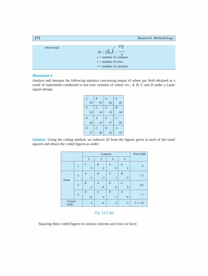
Illustration 4
Analyse and interpret the following statistics concerning output of wheat per field obtained as a
result of experiment conducted to test four varieties of wheat viz., A, B, C and D under a Latin-
square design.
C
25
B
23
A
20
D
20
A
19
D
19
C
21
B
18
B
19
A
14
D
17
C
20
D
17
C
20
B
21
A
15
Solution: Using the coding method, we subtract 20 from the figures given in each of the small
squares and obtain the coded figures as under:
Columns Row totals
1 2 3 4
1 C
5
B
3
A
0
D
0
8
Rows
2 A
–1
D
–1
C
1
B
–2
–2
3 B
–1
A
–6
D
–3
C
0
–10
4 D
–3
C
0
B
1
A
–5
–7
Column totals
0 –4 –1 –7 T = –12
Fig. 11.2 (a)
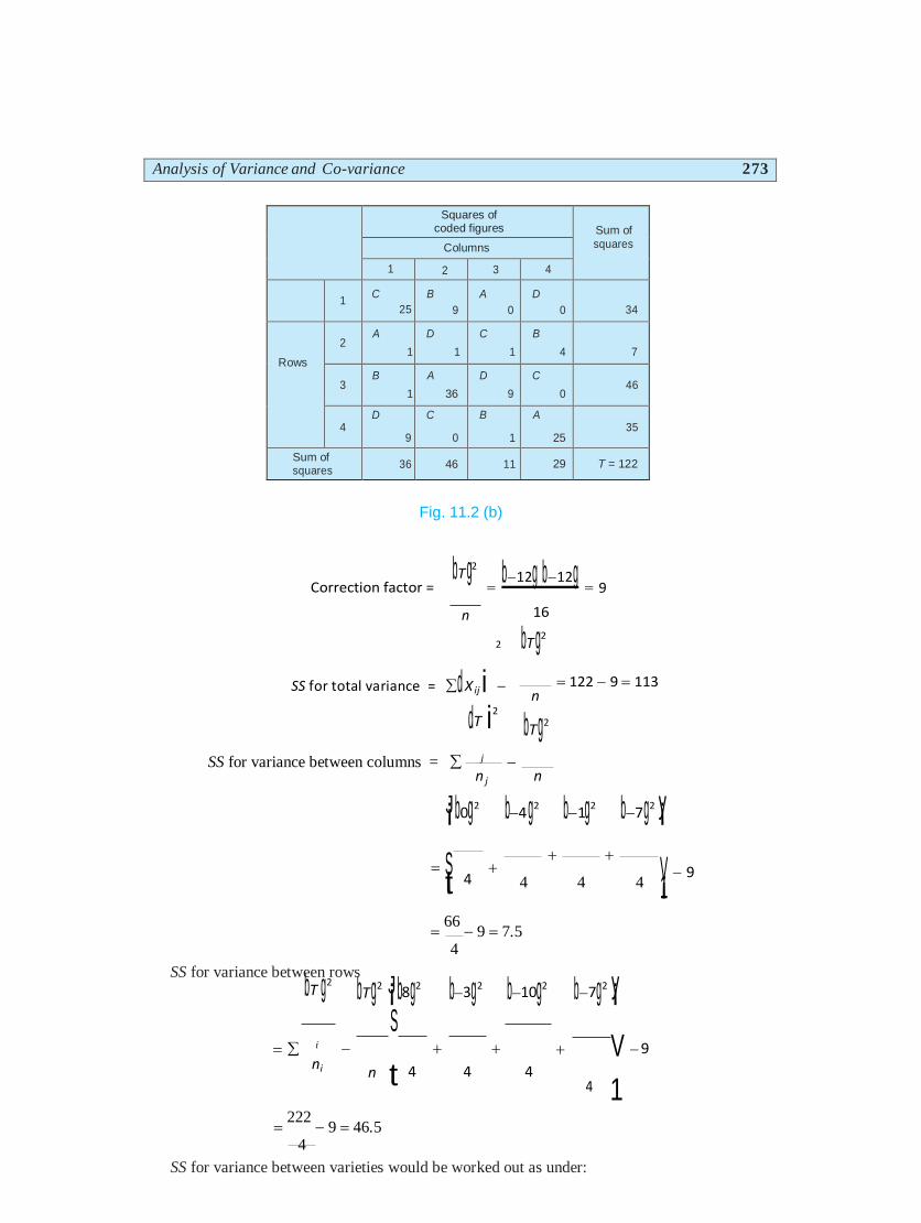
Squaring these coded figures in various columns and rows we have:
¡ ¡ S
Analysis of Variance and Co-variance 273
Squares of
coded figures
Sum of
squares Columns
1 2 3 4
1 C
25
B
9
A
0
D
0
34
Rows
2 A
1
D
1
C
1
B
4
7
3 B
1
A
36
D
9
C
0
46
4 D
9
C
0
B
1
A
25
35
Sum of squares
36 46 11 29 T = 122
Fig. 11.2 (b)
Correction factor =
bT g2
n
b12g b12g
9
16
2 bT g2
SS for total variance = d X ij i
dT i2
n
bTg2
122 9 113
SS for variance between columns = j n j n
J¡b0g2 b4g2 b1g2 b7g2 y¡
S¡t 4
4 4 4 V¡1 9
SS for variance between rows
66
9 7.5 4
bT g2 bTg2 J¡b8g2 b3g2 b10g2
b7g2 y¡
i ni
n t 4 4 4
V 9
4 1
222
9 46.5 4
SS for variance between varieties would be worked out as under:
274 Research Methodology
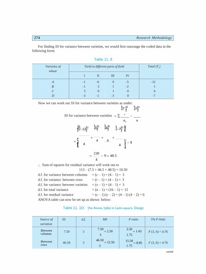
For finding SS for variance between varieties, we would first rearrange the coded data in the
following form:
Table 11. 9
Varieties of
wheat
Yield in different parts of field Total (Tv)
I II III IV
A
B
C
D
–1
–1
5
–3
–6
3
0
–1
0
1
1
–3
–5
–2
0
0
–12
1
6
–7
Now we can work out SS for variance between varieties as under:
bT g2 bT g2
SS for variance between varieties v
nv n
J¡b12g2 b1g2 b6g2
b7g2 y¡
S¡t 4
4 4
4 V¡1 9
230
9 48.5 4
Sum of squares for residual variance will work out to
113 – (7.5 + 46.5 + 48.5) = 10.50
d.f. for variance between columns = (c – 1) = (4 – 1) = 3
d.f. for variance between rows = (r – 1) = (4 – 1) = 3
d.f. for variance between varieties = (v – 1) = (4 – 1) = 3
d.f. for total variance = (n – 1) = (16 – 1) = 15
d.f. for residual variance = (c – 1) (c – 2) = (4 – 1) (4 – 2) = 6
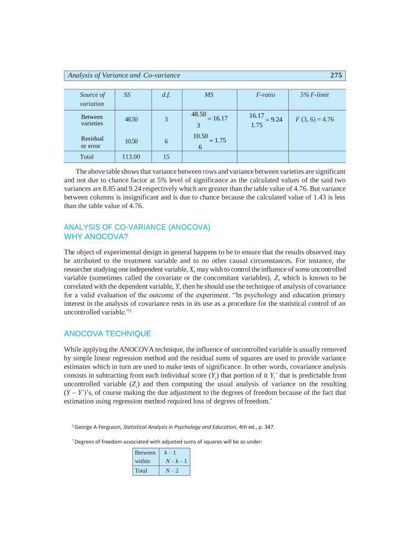
ANOVA table can now be set up as shown below:
Table 11. 1O: †he Anova †able in Latin-square Design
Source of
variation
SS d.f. MS F-ratio 5% F-limit
Between columns
7.50 3 7.50
2.50 3
2.50 1.43
1.75 F (3, 6) = 4.76
Between rows
46.50 3 46.50
15.50 3
15.50 8.85
1.75 F (3, 6) = 4.76
contd.
Analysis of Variance and Co-variance 275
Source of
variation
SS d.f. MS F-ratio 5% F-limit
Between varieties
48.50
10.50
3
6
48.50 16.17
3
10.50 1.75
6
16.17 9.24
1.75 F (3, 6) = 4.76
Residual
or error
Total 113.00 15
The above table shows that variance between rows and variance between varieties are significant
and not due to chance factor at 5% level of significance as the calculated values of the said two
variances are 8.85 and 9.24 respectively which are greater than the table value of 4.76. But variance
between columns is insignificant and is due to chance because the calculated value of 1.43 is less
than the table value of 4.76.
ANALYSIS OF CO-VARIANCE (ANOCOVA)
WHY ANOCOVA?
The object of experimental design in general happens to be to ensure that the results observed may
be attributed to the treatment variable and to no other causal circumstances. For instance, the
researcher studying one independent variable, X, may wish to control the influence of some uncontrolled
variable (sometimes called the covariate or the concomitant variables), Z, which is known to be
correlated with the dependent variable, Y, then he should use the technique of analysis of covariance
for a valid evaluation of the outcome of the experiment. “In psychology and education primary
interest in the analysis of covariance rests in its use as a procedure for the statistical control of an
uncontrolled variable.”2
ANOCOVA TECHNIQUE
While applying the ANOCOVA technique, the influence of uncontrolled variable is usually removed
by simple linear regression method and the residual sums of squares are used to provide variance
estimates which in turn are used to make tests of significance. In other words, covariance analysis
consists in subtracting from each individual score (Yi) that portion of it Y
i´ that is predictable from
uncontrolled variable (Zi) and then computing the usual analysis of variance on the resulting
(Y – Y´)’s, of course making the due adjustment to the degrees of freedom because of the fact that
estimation using regression method required loss of degrees of freedom.*
2 George A-Ferguson, Statistical Analysis in Psychology and Education, 4th ed., p. 347.
* Degrees of freedom associated with adjusted sums of squares will be as under:
Between
within
k – 1
N – k – 1
Total N – 2
276 Research Methodology
ASSUMPTIONS IN ANOCOVA
The ANOCOVA technique requires one to assume that there is some sort of relationship between
the dependent variable and the uncontrolled variable. We also assume that this form of relationship is
the same in the various treatment groups. Other assumptions are:
(i) Various treatment groups are selected at random from the population.
(ii) The groups are homogeneous in variability.
(iii) The regression is linear and is same from group to group.
The short-cut method for ANOCOVA can be explained by means of an example as shown
below:
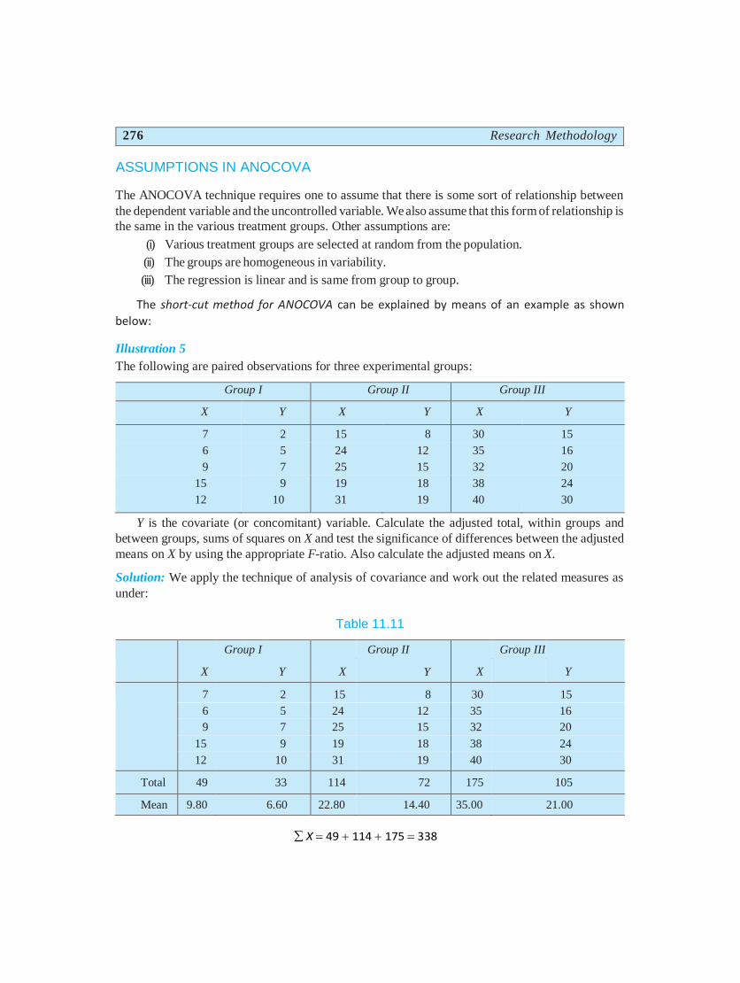
Illustration 5
The following are paired observations for three experimental groups:
Group I Group II Group III
X Y X Y X Y
7 2 15 8 30 15
6 5 24 12 35 16
9 7 25 15 32 20
15 9 19 18 38 24
12 10 31 19 40 30
Y is the covariate (or concomitant) variable. Calculate the adjusted total, within groups and
between groups, sums of squares on X and test the significance of differences between the adjusted
means on X by using the appropriate F-ratio. Also calculate the adjusted means on X.
Solution: We apply the technique of analysis of covariance and work out the related measures as
under:
Table 11.11
X
Group I
Y
X
Group II
Y
X
Group III
Y
7 2 15 8 30 15
6 5 24 12 35 16
9 7 25 15 32 20
15 9 19 18 38 24
12 10 31 19 40 30
Total 49 33 114 72 175 105
Mean 9.80 6.60 22.80 14.40 35.00 21.00
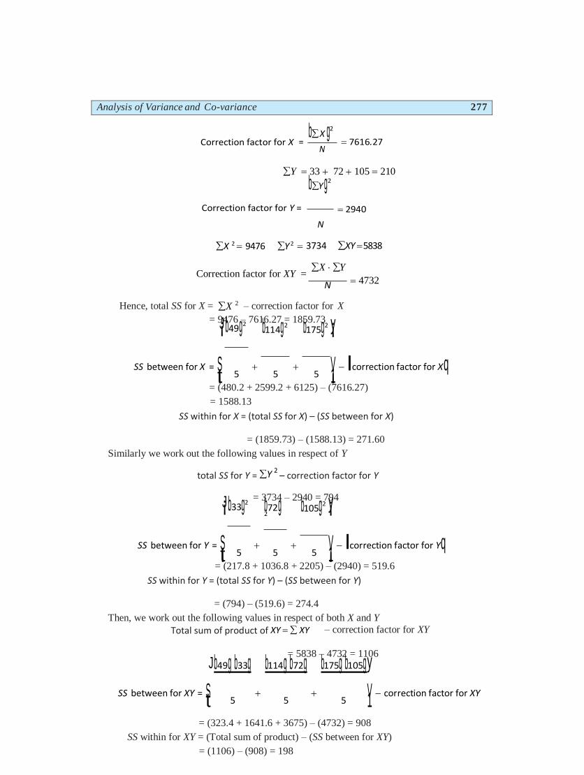
X 49 114 175 338
Analysis of Variance and Co-variance 277
Correction factor for X
b X g2
N
7616.27
Y 33 72 105 210
bY g2
Correction factor for Y =
N
2940
X 2 9476 Y 2 3734 XY 5838
Correction factor for XY = X Y
N
Hence, total SS for X = X 2 – correction factor for X
= 9476 – 7616.27 = 1859.73
4732
J¡b49g2 b114g2 b175g2 y¡
SS between for X = S¡t 5
5
5 V¡1 lcorrection factor for X q
= (480.2 + 2599.2 + 6125) – (7616.27)
= 1588.13
SS within for X = (total SS for X) – (SS between for X)
= (1859.73) – (1588.13) = 271.60
Similarly we work out the following values in respect of Y
total SS for Y = Y 2 – correction factor for Y
= 3734 – 2940 = 794 J¡b33g2 b72g
2
b105g2 y¡
SS between for Y = S¡t 5
5
5 V¡1 lcorrection factor for Yq
= (217.8 + 1036.8 + 2205) – (2940) = 519.6
SS within for Y = (total SS for Y) – (SS between for Y)
= (794) – (519.6) = 274.4
Then, we work out the following values in respect of both X and Y
Total sum of product of XY XY – correction factor for XY
= 5838 – 4732 = 1106 Jb49g b33g b114g b72g b175g b105gy
SS between for XY = St 5
5
5 V1 correction factor for XY
= (323.4 + 1641.6 + 3675) – (4732) = 908
SS within for XY = (Total sum of product) – (SS between for XY)
= (1106) – (908) = 198
=
278 Research Methodology
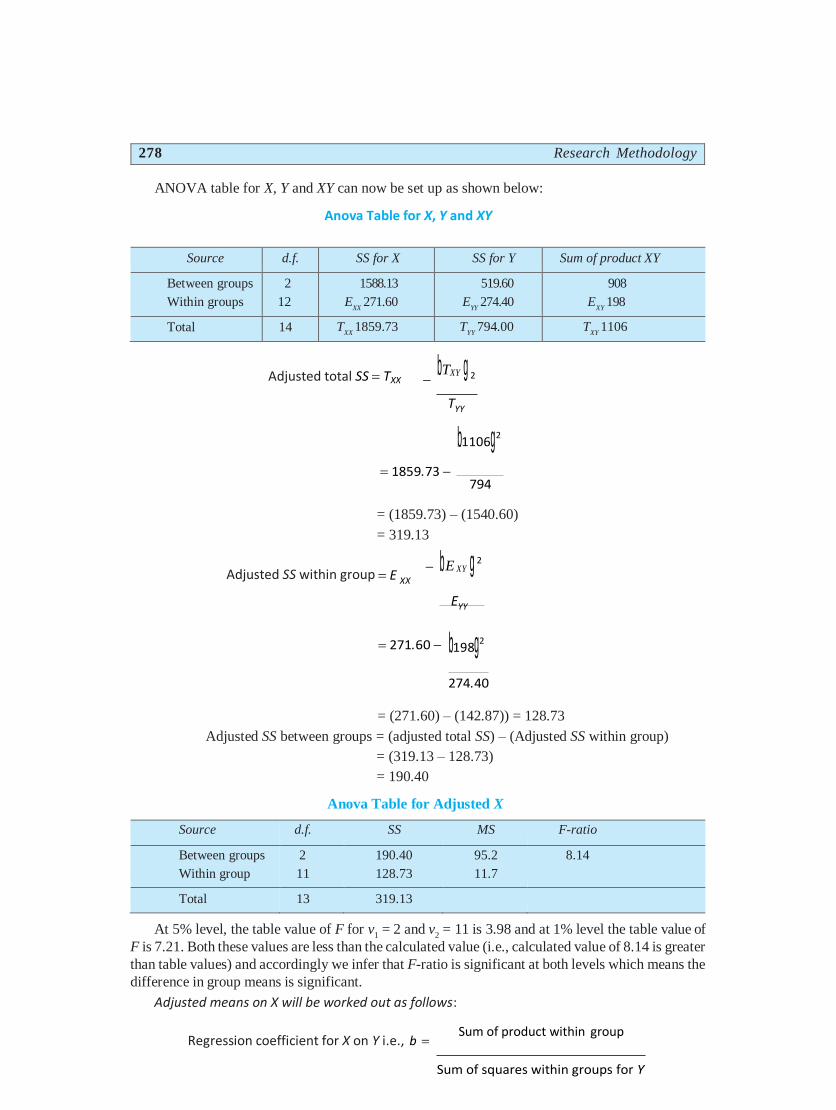
ANOVA table for X, Y and XY can now be set up as shown below:
Anova Table for X, Y and XY
Source d.f. SS for X SS for Y Sum of product XY
Between groups
Within groups
2
12
1588.13
EXX
271.60
519.60
EYY
274.40
908
EXY
198
Total 14 TXX
1859.73 TYY
794.00 TXY
1106
Adjusted total SS TXX
bTXY g TYY
b1106g2
1859.73 794
= (1859.73) – (1540.60)
= 319.13
Adjusted SS within group E XX
bE XY g
271.60
EYY
b198g2
274.40
= (271.60) – (142.87)) = 128.73
Adjusted SS between groups = (adjusted total SS) – (Adjusted SS within group)
= (319.13 – 128.73)
= 190.40
Anova Table for Adjusted X
Source d.f. SS MS F-ratio
Between groups 2 190.40 95.2 8.14
Within group 11 128.73 11.7
Total 13 319.13
At 5% level, the table value of F for v1
= 2 and v2
= 11 is 3.98 and at 1% level the table value of
F is 7.21. Both these values are less than the calculated value (i.e., calculated value of 8.14 is greater
than table values) and accordingly we infer that F-ratio is significant at both levels which means the
difference in group means is significant.
Adjusted means on X will be worked out as follows:
Regression coefficient for X on Y i.e., b Sum of product within group
Sum of squares within groups for Y
2
2
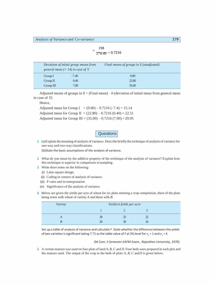
Analysis of Variance and Co-variance 279
198
274.40 0.7216
Deviation of initial group means from Final means of groups in X (unadjusted)
general mean (= 14) in case of Y
Group I –7.40 9.80
Group II 0.40 22.80
Group III 7.00 35.00
Adjusted means of groups in X = (Final mean) – b (deviation of initial mean from general mean
in case of Y)
Hence,
Adjusted mean for Group I = (9.80) – 0.7216 (–7.4) = 15.14
Adjusted mean for Group II = (22.80) – 0.7216 (0.40) = 22.51
Adjusted mean for Group III = (35.00) – 0.7216 (7.00) = 29.95
1. (a) Explain the meaning of analysis of variance. Describe briefly the technique of analysis of variance for
one-way and two-way classifications.
(b)State the basic assumptions of the analysis of variance.
2. What do you mean by the additive property of the technique of the analysis of variance? Explain how
this technique is superior in comparison to sampling.
3. Write short notes on the following:
(i) Latin-square design.
(ii) Coding in context of analysis of variance.
(iii) F-ratio and its interpretation.
(iv) Significance of the analysis of variance.
4. Below are given the yields per acre of wheat for six plots entering a crop competition, there of the plots
being sown with wheat of variety A and three with B.
Variety
1
Yields in fields
2
per acre
3
A
B
30
20
32
18
22
16
Set up a table of analysis of variance and calculate F. State whether the difference between the yields of two varieties is significant taking 7.71 as the table value of F at 5% level for v
1 = 1 and v
2 = 4.
(M.Com. II Semester EAFM Exam., Rajasthan University, 1976)
5. A certain manure was used on four plots of land A, B, C and D. Four beds were prepared in each plot and
the manure used. The output of the crop in the beds of plots A, B, C and D is given below:
Questions
280 Research Methodology
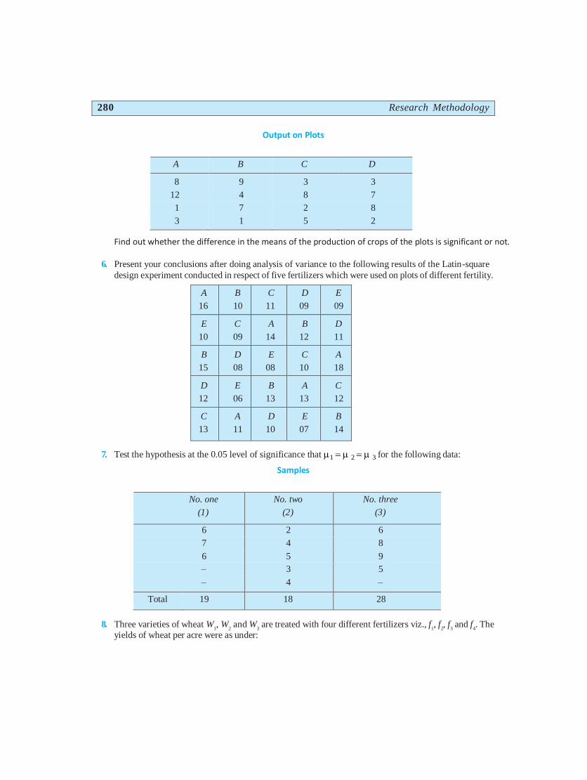
Output on Plots
A B C D
8 9 3 3
12 4 8 7
1 7 2 8
3 1 5 2
Find out whether the difference in the means of the production of crops of the plots is significant or not.
6. Present your conclusions after doing analysis of variance to the following results of the Latin-square
design experiment conducted in respect of five fertilizers which were used on plots of different fertility.
A
16
B
10
C
11
D
09
E
09
E
10
C
09
A
14
B
12
D
11
B
15
D
08
E
08
C
10
A
18
D
12
E
06
B
13
A
13
C
12
C
13
A
11
D
10
E
07
B
14
7. Test the hypothesis at the 0.05 level of significance that 1 2 3 for the following data:
Samples
No. one
(1)
No. two
(2)
No. three
(3)
6 2 6
7 4 8
6 5 9
– 3 5
– 4 –
Total 19 18 28
8. Three varieties of wheat W1, W
2 and W
3 are treated with four different fertilizers viz., f
1, f
2, f
3 and f
4. The
yields of wheat per acre were as under:
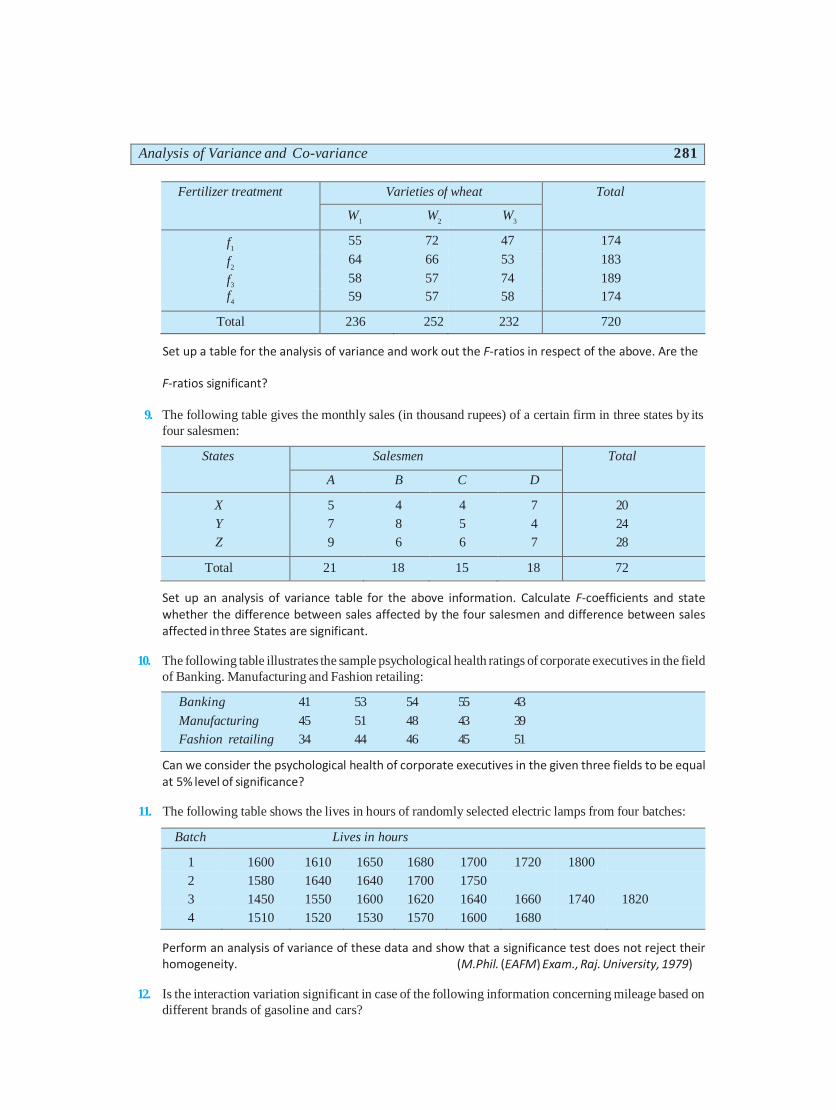
Analysis of Variance and Co-variance 281
Fertilizer treatment Varieties of wheat Total
W1
W2
W3
f1
55 72 47 174
f2
64 66 53 183
f3 58 57 74 189
f4
59 57 58 174
Total 236 252 232 720
Set up a table for the analysis of variance and work out the F-ratios in respect of the above. Are the
F-ratios significant?
9. The following table gives the monthly sales (in thousand rupees) of a certain firm in three states by its
four salesmen:
States Salesmen Total
A B C D
X
Y
Z
5
7
9
4
8
6
4
5
6
7
4
7
20
24
28
Total 21 18 15 18 72
Set up an analysis of variance table for the above information. Calculate F-coefficients and state whether the difference between sales affected by the four salesmen and difference between sales affected in three States are significant.
10. The following table illustrates the sample psychological health ratings of corporate executives in the field
of Banking. Manufacturing and Fashion retailing:
Banking 41 53 54 55 43
Manufacturing 45 51 48 43 39
Fashion retailing 34 44 46 45 51
Can we consider the psychological health of corporate executives in the given three fields to be equal at 5% level of significance?
11. The following table shows the lives in hours of randomly selected electric lamps from four batches:
Batch Lives in hours
1 1600 1610 1650 1680 1700 1720 1800
2 1580 1640 1640 1700 1750
3 1450 1550 1600 1620 1640 1660 1740 1820
4 1510 1520 1530 1570 1600 1680
Perform an analysis of variance of these data and show that a significance test does not reject their homogeneity. (M.Phil. (EAFM) Exam., Raj. University, 1979)
12. Is the interaction variation significant in case of the following information concerning mileage based on
different brands of gasoline and cars?
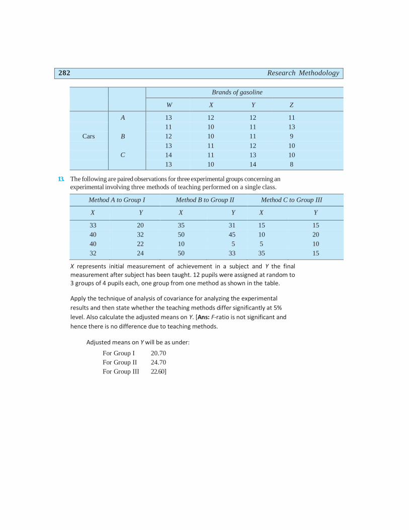
282 Research Methodology
Brands of gasoline
W X Y Z
A
B
C
13 12 12 11
11 10 11 13
Cars 12 10 11 9
13 11 12 10
14 11 13 10
13 10 14 8
13. The following are paired observations for three experimental groups concerning an
experimental involving three methods of teaching performed on a single class.
Method A to Group I Method B to Group II Method C to Group III
X Y X Y X Y
33 20 35 31 15 15
40 32 50 45 10 20
40 22 10 5 5 10
32 24 50 33 35 15
X represents initial measurement of achievement in a subject and Y the final
measurement after subject has been taught. 12 pupils were assigned at random to 3 groups of 4 pupils each, one group from one method as shown in the table.
Apply the technique of analysis of covariance for analyzing the experimental
results and then state whether the teaching methods differ significantly at 5%
level. Also calculate the adjusted means on Y. [Ans: F-ratio is not significant and
hence there is no difference due to teaching methods.
Adjusted means on Y will be as under:
For Group I 20.70
For Group II 24.70
For Group III 22.60]