1

STATISTICS

Analysis Of Variance

Review Preview ANOVA

F test One-way ANOVA Multiple comparison Two-way ANOVA

2

STATISTICS

),(~ 2Nx

x

Zx

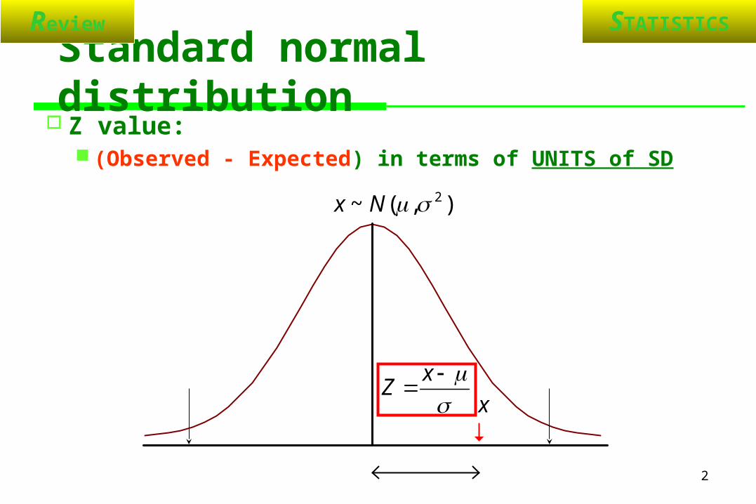
Standard normal distribution Z value:

(Observed - Expected) in terms of UNITS of SD

Review

3

STATISTICS

Central Limit Theorem Review

)/,(~ 2 nNx

),(~ 2Nx

For large n,

X

The beauty of CLT: Easy to calculate V

The ugliness of CLT: Hard to explain p

4

STATISTICS

Sampling Distribution of

)( 21 xx

),(~2

22

1

21

2121nn

Nxx

2

)/,(~ 22222 nNx

21 21 xx

1

)/,(~ 12111 nNx

2

)( 21 xx

)( 21 xx

Review

5

STATISTICS

Population & Sampling Distribution

Review

Population parameters known Population parameters unknown

Mean SD Z score Mean SD t score

x N

xi N

xi

2)(

Xz n

xx i

1

)( 2

n

xxS i

S

xxt

x N

xi

x n

SEx

n

xZ i

x )(

n

xi

x n

SSE

x

nSx

t ix

)(

Please add yourself: )( 21 xx

STATISTICS

No of groups

N > 30

ND

1-s t

1-s t

1. TransF for t 2. sign test

N > 30

Independent

N > 30

ND

ND

Equal variance 2-s t

2-s t

2-s t

1. transform for t 2. WRS test

1. TransF for t 2. WRS test

Paired t

Paired t

1. transform for t 2. WSR test

Equal N

1 group

2 group

If Yes, go up; If No, do down

Flowchart of 2G MD testReview

7

STATISTICS

ANOVA

Analysis of Variance

8

STATISTICS

Analysis of Variance

The logic of ANOVA Partition of sum of squares

F test One way ANOVA

Multiple comparison Two way ANOVA

Interaction and confounding

ANOVA

9

STATISTICS

Eyeball test for 3-sample means

ANOVA

A B

Using 95% Confidence Limits A: Non-Significant B: Significant

Why? Between group variation Within group variation

Why not do 2-s test 3 times? Alpha error inflated Ex: 7 groups MD comparisons

1 / 21 < 0.05 !!

1 2 3 1 2 3

10

STATISTICS

Data sheet: k groups MD comparison

Subjects Observed Tx Group

Mean

Grand

Mean

Group

Effect Tx error

Total

Difference

1 X1 X1-Ma X1-M

2 X2 X2-Ma X2-M

3 X3

A Ma Ma-M

X3-Ma X3-M

4 X4

5 X5 B Mb Mb-M

… … … … …

… …

n Xn K Mk

M

Mk-M

ANOVA

11

STATISTICS

The Logic of one-way ANOVA

Total Difference divided into two parts (Observed－ group mean)＋ (group mean－ grand mean)

Total sum of squares divided into two parts SS Total = SS Between + SS Within (or Error) SST = SSB + SSE

Partition of TD & TSS Model of one-way ANOVA

j i

j

j i

jijj i

jjijj i

ij XXXXXXXXXX 2.

2.

2..

2 )()()]()[()(

ANOVA

)()( .. XXXXXX jjijij

ijjij eX

A B C

x

x

x

12

STATISTICS

Assumptions in ANOVA

Normal Distribution: Y values in each group Not very important, esp. for large n If not ND and small n: Kruskal-Wallis nonparametric

Equal variance: homogeneity If not: data transformation or ask for help

Random & independent sample

13

STATISTICS

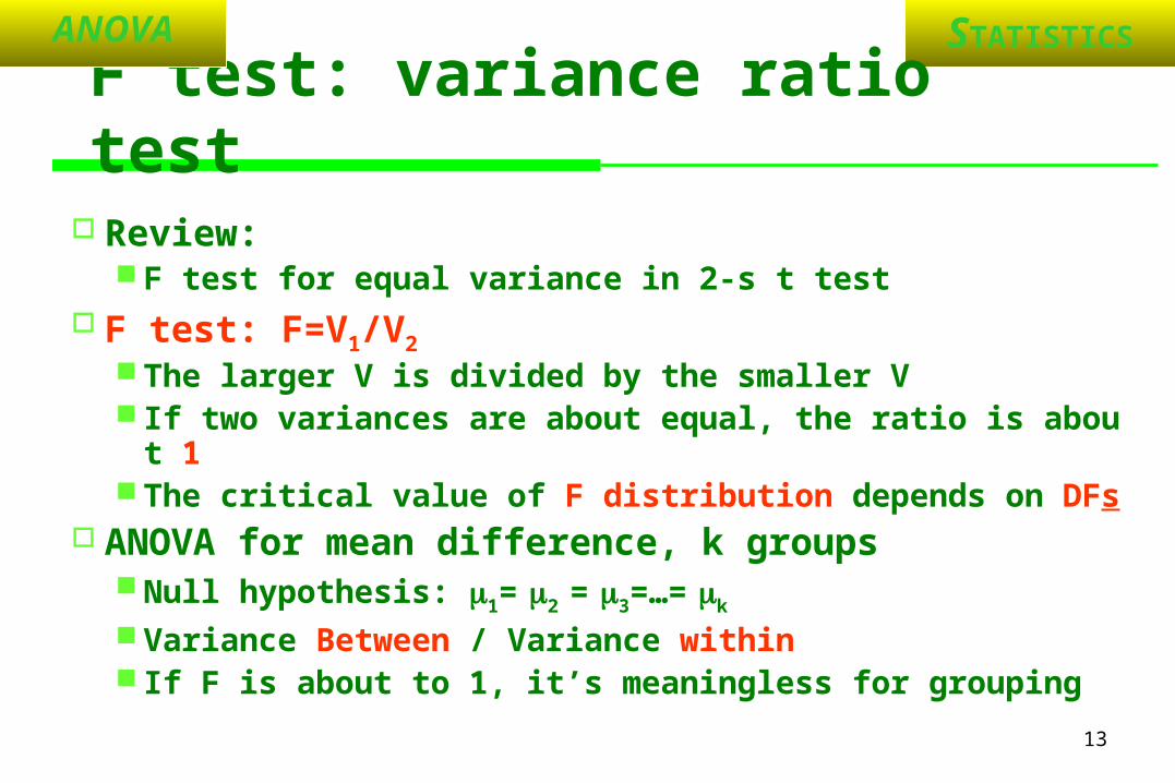
F test: variance ratio test

Review: F test for equal variance in 2-s t test

F test: F=V1/V2

The larger V is divided by the smaller V If two variances are about equal, the ratio is about 1 The critical value of F distribution depends on DFs

ANOVA for mean difference, k groups Null hypothesis: 1= 2 = 3=…= k

Variance Between / Variance within If F is about to 1, it’s meaningless for grouping

ANOVA

14

STATISTICS

F test : named after Fisher Characteristics

a sickly, poor-eyesighted child The teacher used no paper/pencil t

o teach him Very strong instinct on geometry Mathematicians take years to prove

his formulas Persistence

Calculation of ANOVA tables takes Fisher 8 months, 8h/D to finish!!

Reference: The lady tasting tea, Salsburg, 2001 「統計，改變了世界」天下， 2001

Sir Ronald Aylmer Fisher 1890-1962

ANOVA

15

STATISTICS

One-way ANOVA

ANOVA

16

STATISTICS

One-way ANOVA table

Source of variation SS DF Mean SS F ratio

Between k groups SSB k-1 MSB MSB/MSE

Error(within groups) SSE n-k MSE

Total SST n-1

F test:)/(

)1/(

knSSE

kSSB

MESS

MBSS

MS

MSF

E

B

ANOVA

17

STATISTICS

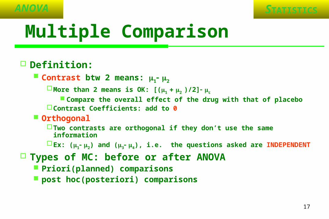
Multiple Comparison

Definition: Contrast btw 2 means: 1 2

More than 2 means is OK: [(1 2 )/2] c

Compare the overall effect of the drug with that of placeboContrast Coefficients: add to 0

OrthogonalTwo contrasts are orthogonal if they don’t use the same informationEx: (1 2) and (3 4), i.e. the questions asked are INDEPENDENT

Types of MC: before or after ANOVA Priori(planned) comparisons post hoc(posteriori) comparisons

ANOVA

18

STATISTICS

Research problem: Life events, depressive symptoms, and immune function. Irwin

M. Am J Psychiatry, 1987; 144:437-441

Subjects: women whose husbands treated for lung Ca.died of lung Ca. in the preceding 1-6 Monthswere in good health

X: grouping by scores for major life events Measurement: Social Readjustment Rating Scale score

Y: immune system functionNK cell activity: lytic units

Example 1: one-way ANOVA

ANOVA

19

STATISTICS

Box plot & Error bar plot

0.00

25.00

50.00

75.00

100.00

1 2 3

Box Plot

GROUP

CE

LL

10.0

15.6

21.1

26.7

32.2

37.8

43.3

48.9

54.4

60.0

1 2 3

Error Bar Plot

Printout

20

STATISTICS

ANOVA table

Analysis of Variance Table

Source Term DF Sum of Squares Mean Square F-Ratio Prob Power(Alpha=0.05)

A: GROUP 2 4654.156 2327.078 8.35 0.001125* 0.947488

S(A) 34 9479.396 278.8058

Total (Adjusted) 36 14133.55

Total 37

Printout

21

STATISTICS

Nonparametric ANOVA

Printout

Kruskal-Wallis One-Way ANOVA on Ranks Test Results

Method DF Chi-Sq (H) Prob. Level Decision (0.05)

Not Corrected for Ties 2 11.16963 0.003754 Reject Ho

Corrected for Ties 2 11.17095 0.003752 Reject Ho

Group Detail

Group Count Sum of Ranks Mean Rank Z-Value Median

1 13 351.00 27.00 3.3087 37

2 12 163.50 13.63 -2.0927 14.5

3 12 188.50 15.71 -1.2815 14.05

22

STATISTICS

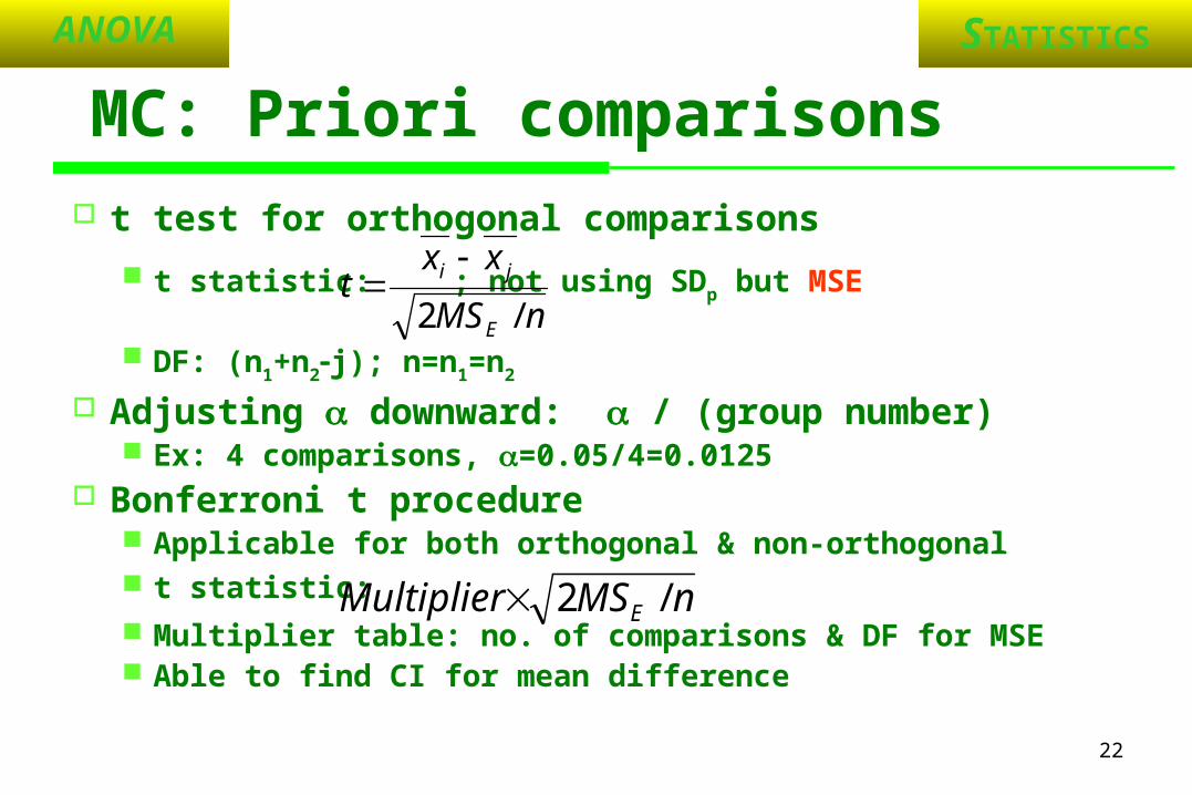
MC: Priori comparisons t test for orthogonal comparisons

t statistic: ; not using SDp but MSE

DF: (n1+n2j); n=n1=n2

Adjusting downward: / (group number) Ex: 4 comparisons, =0.05/4=0.0125

Bonferroni t procedure Applicable for both orthogonal & non-orthogonal t statistic:

Multiplier table: no. of comparisons & DF for MSE Able to find CI for mean difference

nMS

xxt

E

ji

/2

nMSMultiplier E /2

ANOVA

23

STATISTICS

MC: Posteriori comparisons

Tukey’s HSD (honestly significant difference) HSD=

Like Bonferroni, HSD multiplier table is needed (P176, table 7-7) Able to find CI for mean difference

Ex:

n

MSMultiplier E

ANOVA

31.2112

82.27842.4 HSD

24.63 22.17

2.46

LOWn=13

MODn=12

HIGHn=12

24

STATISTICS

MC: Posteriori comparisons Scheffé’s procedure

S statistic:

j: No. of groups; C: contrast; (alpha, df1, df2)=(0.01, 2, 34)

most versatile (not only pair-wise) & most conservativeEX: Low (Moderate & High) combined; Low Moderate

Note: MD btw L & H not significant Able to find CI for mean difference

j

jEdf n

CMSFjS

2

,)1(

ANOVA

167.012

)1(

12

1;125.0

12

)5.0(

12

)5.0(

12

1 2222222

j

j

j

j

n

C

n

C

24.22167.082.27831.5)13( S

25

STATISTICS

MC: Posteriori comparisons

Newman-Keuls procedure NK statistic:

Multiplier table is needed Less conservative than Tukey’s HSD Unable to find CI for mean difference Ex:2 steps ; 3 steps

n

MSmultiplier E

3 Steps

2 Steps 2 Steps

ANOVA

65.1882.487.3 NK 31.2182.442.4 NK

same as HSD

26

STATISTICS

MC: Posteriori comparisons

Dunnett’s procedure Dunnett’s statistic:

Only used in several Tx means with single CTL mean Relatively low critical value Ex:

2 units lower than HSD value; 4 units lower than Scheffé value

n

MSmultiplier E2

ANOVA

48.1882.671.2 D

27

STATISTICS

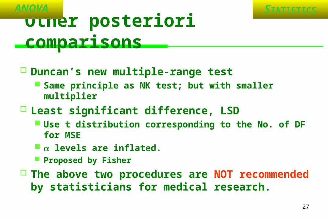
Other posteriori comparisons

Duncan’s new multiple-range test Same principle as NK test; but with smaller multiplier

Least significant difference, LSD Use t distribution corresponding to the No. of DF for MSE levels are inflated. Proposed by Fisher

The above two procedures are NOT recommended by statisticians for medical research.

ANOVA

28

STATISTICS

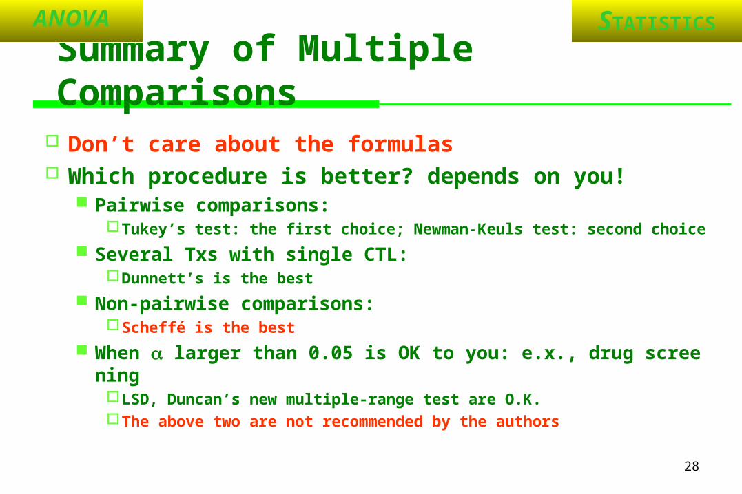
Summary of Multiple Comparisons

Don’t care about the formulas Which procedure is better? depends on you!

Pairwise comparisons: Tukey’s test: the first choice; Newman-Keuls test: second choice

Several Txs with single CTL: Dunnett’s is the best

Non-pairwise comparisons:Scheffé is the best

When larger than 0.05 is OK to you: e.x., drug screeningLSD, Duncan’s new multiple-range test are O.K.The above two are not recommended by the authors

ANOVA

29

STATISTICS

Multiple comparisonsNewman-Keuls Multiple-Comparison Test

Group Count Mean Different From Groups

2 12 15.60000 1

3 12 18.05833 1

1 13 40.23077 2, 3

Response: CELL; Term A: GROUP; DF=34; MSE=278.8058

Scheffe's Multiple-Comparison Test

Group Count Mean Different From Groups

2 12 15.60000 1

3 12 18.05833 1

1 13 40.23077 2, 3

Critical Value=2.5596

Printout

30

STATISTICS

Two-way ANOVA

ANOVA

31

STATISTICS

The Logic of two-way ANOVA

SST divided into 3 or 4 parts SST = SSR + SSC + SSE SST = SSR + SSC + SS(RC) +SSE

Models of two-way ANOVA Without interaction:

With interaction:

ANOVA

ijjiij eX

ijjijiij eX )(

32

STATISTICS

Simpson’s Paradox: 陳小姐買帽子

 

第一天 第二天

第一櫃 (大人 ) 第二櫃 (小孩 ) 兩櫃一起

紅色 黑色 紅色 黑色 紅色 黑色

合適 9 17 3 1 12 18

不合適 1 3 17 9 18 12

Total 10 20 20 10 30 30

 90% 85% 15% 10% 40% 60%

ANOVA

33

STATISTICS

Statistical Interaction & confounding

Interaction: 2 lines with different slope

Confounding: 2 parallel lines

T0 T1

C1

C0

Y

C0

C1

1|11ˆˆ: cH

TCCTCTY 321,|

How to test: ANOVA

ANOVA

0ˆ: 31 H

34

STATISTICS

Confounding factors

Mixing effect of X2 with X1 & Y Definition:

Associated With the disease of interest in the absence of exposure

本身單獨與疾病有相關；本身是危險因子 Associated With the exposure

與危險因子有相關 Not as a result of being exposed.

干擾不能是中介變項： intervening variable Intervening variable: X1X2YExample: S/S of diseases

MI

Obesity

Cholesterol

ANOVA

35

STATISTICS

Interaction & confounding

Interaction: The effect of X1 varies with the level of X2 A phenomenon you have to present Main effects of X1, X2: not meaningful anymore Ex: X1(Sex), X2(teaching method) & Y (language score)

Confounding: Given condition: no interaction A condition you have to control (or adjust)

ANOVA

36

STATISTICS

Two-way ANOVA table

Source of variation SS DF Mean SS F ratio

Among rows SSR r-1 MSR MSR/MSE

Among columns SSC c-1 MSC MSC/MSE

Interaction SS(RC) (r-1)(c-1) MS(RC) MS(RC)/MSE

Error SSE rc(n-1) MSE

Total SST n-1

ANOVA

37

STATISTICS

Example 2: two-way ANOVA

Research problem: Glucose tolerance, insulin secretion, insulin sensitivi

ty and glucose effectiveness in normal and overweight hyperthyroid women. Gonzalo MA. Clin Endocrinol, 1996;45:689-697

X1: BMI; X2: thyroid functionAll categorical variablesBMI: 2 level; thyroid function: 2 level;

Y: Insulin sensitivityContinuous variable

ANOVA

38

STATISTICS

Box plot & Error bar plot, ex 2

0.00

0.25

0.50

0.75

1.00

0 1

Means of IS

BMI2

IS

HT

01

0.0

0.1

0.2

0.3

0.4

0.6

0.7

0.8

0.9

1.0

0 1

Error Bar Plot

BMI

IS

HT

0 Normal thyroid1 Hyperthyroid

Printout

39

STATISTICS

Descriptive statistics, ex 2Means and Standard Errors of IS

Term Count Mean SE

All 33 0.4647917

A: BMI2

0 19 0.615 5.786324E-02

1 14 0.3145833 6.740864E-02

B: HT

0 19 0.57375 5.786324E-02

1 14 0.3558333 6.740864E-02

AB: BMI2,HT

0,0 11 0.68 0.0760472

0,1 8 0.55 8.917324E-02

1,0 8 0.4675 8.917324E-02

1,1 6 0.1616667 0.1029684

Printout

40

STATISTICS

2-way ANOVA table, ex 2

Analysis of Variance Table for IS (alpha = 0.05)

Source DF SS MSS F-Ratio Prob. Power

A: BMI2 1 0.7112253 0.7112253 11.18 0.002293* 0.898154

B: HT 1 0.3742312 0.3742312 5.88 0.021745* 0.649738

AB 1 6.091182E-02 6.091182E-02 0.96 0.335909 0.157220

S 29 1.844833 6.361494E-02

Total (Adj.) 32 2.916255

Total 33

Printout

41

STATISTICS

Flowchart of 3G MD test

Indepedent

ND

No. of Factors

One-way ANOVA

Two-way ANOVAor other

ND

RepeatedANOVA

Friedman

1 Factor

2 or more Factors

Kruskal-Wallisfor 1 Factor

3 or more groups

Summary

If Yes, go up; If No, do down

42

STATISTICS

QUIZ

Q: Can I use ANOVA to test 2G MD? A: Yes, you can. Q: What is the relationship btw ANOVA & 2-s t? A: 2-s t test is a special case of ANOVA F, t & Z table:

22/1),1(,2

2

)1(,2/1)1,1(,

,).2(

).1(22

ZFdf

tF nn

43

STATISTICS

Home Work Chapter 7, exercise 7, (table 7-20, p187)

Analysis of phenotypic variation in psoriasis as a function of age at onset and family history. Arch. Dermatol. Res. 2002;294:207-213

Answering the following questions: Is there a difference in %TBSA (percent of total body surface area affected) related to age at onset? Is there a difference in %TBSA related to type of psoriasis (familial vs. sporadic)? Is the interaction significant? What is your conclusion?