One-Way and Factorial ANOVA SPSS Lab #3. One-Way ANOVA Two ways to run a one-way ANOVA 1.Analyze Compare Means One-Way ANOVA Use if you have multiple

One-Way and Factorial ANOVA

SPSS Lab #3

One-Way ANOVA

Two ways to run a one-way ANOVA1. Analyze Compare Means One-Way

ANOVA Use if you have multiple DV’s, but only one IV

2. Analyze General Linear Model Univariate

Use if you have only one DV bc/ can provide effect size statistics

More on this later (factorial ANOVA section)

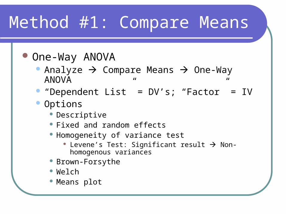
Method #1: Compare Means

First we have to test if we meet the assumptions of ANOVA: Independence of Observations

Cannot be tested statistically, is determined by research methodology only

Normally Distributed DataShapiro-Wilk’s W statistic, if significant, indicates

significant non-normality in dataAnalyze Descriptive Statistics Explore

Click on “Plots”, make sure “Normality Plots w/Tests” is checked

Testing Assumptions

Tests of Normality

.511 111 .000 .371 111 .000

.386 86 .000 .685 86 .000

PESSGRPOptimistic

Pessimistic

BDI214Statistic df Sig. Statistic df Sig.

Kolmogorov-Smirnova

Shapiro-Wilk

Lilliefors Significance Correctiona.

Testing Assumptions

Homogeneity of Variances (Homoscedasticity)

Tested at the same time you test ANOVAAnalyze Compare Means One-Way

ANOVA Click on “Options” and make sure “Homogeneity of

variance test” is checked If violated, use Brown-Forsythe or Welch statistics,

which do not assume homoscedasticity


One-Way ANOVA Analyze Compare Means One-Way ANOVA “Dependent List” = DV’s; “Factor” = IV Options

Descriptive Fixed and random effects Homogeneity of variance test

Levene’s Test: Significant result Non-homogenous variances

Brown-Forsythe Welch Means plot


Descriptives

BDI2TOT

201 11.46 9.921 .700 10.08 12.84 0 49

25 8.88 8.472 1.694 5.38 12.38 0 28

2 8.00 7.071 5.000 -55.53 71.53 3 13

2 4.50 3.536 2.500 -27.27 36.27 2 7

5 19.20 10.232 4.576 6.49 31.91 10 36

235 11.26 9.799 .639 10.00 12.52 0 49

9.756 .636 10.01 12.51

1.682 6.59 15.93 3.262

Caucasian

African American

Asian American

Hispanic

Other

Total

Fixed Effects

Random Effects

Model

N Mean Std. Deviation Std. Error Lower Bound Upper Bound

95% Confidence Interval forMean

Minimum Maximum

Between-Component

Variance

Test of Homogeneity of Variances

BDI2TOT

.403 4 230 .806

LeveneStatistic df1 df2 Sig.

Robust Tests of Equality of Means

BDI2TOT

1.992 4 3.765 .268

2.378 4 10.901 .116

Welch

Brown-Forsythe

Statistica

df1 df2 Sig.

Asymptotically F distributed.a.


RACE

OtherHispanicAsian AmericanAfrican AmericanCaucasian

Me

an

of

BD

I2T

OT

30

20

10

0


One-Way ANOVAPost-Hoc

Can only be done if your IV has 3+ levels Pointless if only 2 levels, just look @ the means

Click the test you want, either with equal variances assumed or not assumed

DON’T just click all of them and see which one gives what you want (that’s cheating), select the test you want priori


ContrastsClick “Polynomial”, Leave “Degree” at default

(“Linear”)

Enter in your coefficients # of coefficients should equal # of levels of your IV

Doesn’t count missing cells, so if you have 3 levels, but no one in one of the levels, you should have 2 coefficients

Coefficients need to sum to 0


ContrastsEnter in your coefficients

IV = Race – 1=Caucasian, 2=African American, 3=Asian American, 4=Hispanic, 5=Native American, 6=Other, BUT there were no Native Americans in the sample

If you want to compare Caucasians to “Other”, coefficients = 1, 0, 0, 0, -1

Caucasians vs. everyone else = -1, .25, .25, .25, .25


ANOVA

BDI2TOT

577.335 4 144.334 1.517 .198

45.416 1 45.416 .477 .490

531.919 3 177.306 1.863 .137

21889.831 230 95.173

22467.166 234

(Combined)

Weighted

Deviation

Linear Term

BetweenGroups

Within Groups

Total

Sum ofSquares df Mean Square F Sig.

Contrast Coefficients

-1 0 0 0 1Contrast1

CaucasianAfrican

AmericanAsian

American Hispanic Other

RACE

Contrast Tests

7.74 4.417 1.753 230 .081

7.74 4.629 1.672 4.189 .167

Contrast1

1

Assume equal variances

Does not assume equalvariances

BDI2TOT

Value ofContrast Std. Error t df Sig. (2-tailed)

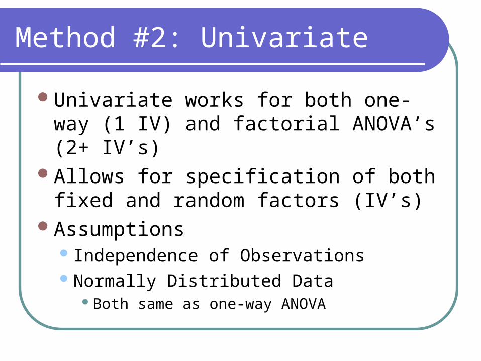
Method #2: Univariate

Univariate works for both one-way (1 IV) and factorial ANOVA’s (2+ IV’s)

Allows for specification of both fixed and random factors (IV’s)

Assumptions Independence of ObservationsNormally Distributed Data

Both same as one-way ANOVA

Factorial ANOVA

Assumptions:Homoscedasticity

Tested at the same time you test ANOVAClick on Analyze General Linear Model

Univariate Click on “Options” and make sure “Homogeneity tests”

is checked

Factorial ANOVA

Options Estimated Marginal Means

Displays means, SD’s, & CI’s for each level of each IV selected

If “Compare main effects” is checked, works as one-way ANOVA on each IV selected

“Confidence interval adjustments” allows you to correct for inflation of alpha using Bonferroni or Sidak method

Descriptive statistics Estimates of effect size Observed power

Pointless, adds nothing to interpretation of p-value and e.s. Homogeneity tests

Levene’s test

Factorial ANOVA

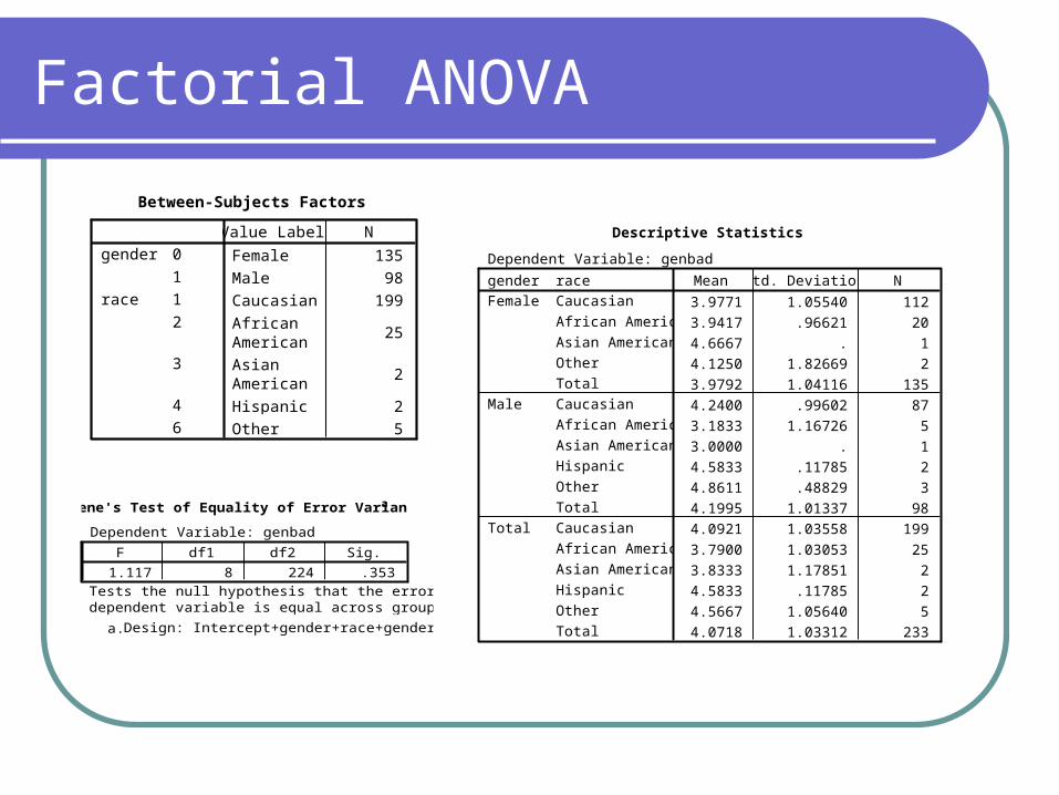
Between-Subjects Factors

Female 135

Male 98

Caucasian 199

AfricanAmerican

25

AsianAmerican

2

Hispanic 2

Other 5

0

1

gender

1

2

3

4

6

race

Value Label N Descriptive Statistics

Dependent Variable: genbad

3.9771 1.05540 112

3.9417 .96621 20

4.6667 . 1

4.1250 1.82669 2

3.9792 1.04116 135

4.2400 .99602 87

3.1833 1.16726 5

3.0000 . 1

4.5833 .11785 2

4.8611 .48829 3

4.1995 1.01337 98

4.0921 1.03558 199

3.7900 1.03053 25

3.8333 1.17851 2

4.5833 .11785 2

4.5667 1.05640 5

4.0718 1.03312 233

raceCaucasian

African American

Asian American

Other

Total

Caucasian

African American

Asian American

Hispanic

Other

Total

Caucasian

African American

Asian American

Hispanic

Other

Total

genderFemale

Male

Total

Mean Std. Deviation N

Levene's Test of Equality of Error Variancesa


1.117 8 224 .353F df1 df2 Sig.

Tests the null hypothesis that the error variance of thedependent variable is equal across groups.

Design: Intercept+gender+race+gender * racea.

Pairwise Comparisons


.546 .267 .419 -.211 1.303

.275 .729 1.000 -1.793 2.343

-.475b .729 1.000 -2.543 1.593

-.384 .474 1.000 -1.729 .960

-.546 .267 .419 -1.303 .211

-.271 .770 1.000 -2.453 1.912

-1.021b .770 1.000 -3.203 1.162

-.931 .534 .829 -2.445 .584

-.275 .729 1.000 -2.343 1.793

.271 .770 1.000 -1.912 2.453

-.750b 1.026 1.000 -3.660 2.160

-.660 .864 1.000 -3.109 1.789

.475c .729 1.000 -1.593 2.543

1.021c .770 1.000 -1.162 3.203

.750c 1.026 1.000 -2.160 3.660

.090c .864 1.000 -2.359 2.539

.384 .474 1.000 -.960 1.729

.931 .534 .829 -.584 2.445

.660 .864 1.000 -1.789 3.109

-.090b .864 1.000 -2.539 2.359

(J) raceAfrican American

Asian American

Hispanic

Other

Caucasian

Asian American

Hispanic

Other

Caucasian

African American

Hispanic

Other

Caucasian

African American

Asian American

Other

Caucasian

African American

Asian American

Hispanic

(I) raceCaucasian

African American

Asian American

Hispanic

Other

MeanDifference

(I-J) Std. Error Sig.a

Lower Bound Upper Bound

95% Confidence Interval forDifference

a

Based on estimated marginal means

Adjustment for multiple comparisons: Bonferroni.a.

An estimate of the modified population marginal mean (J).b.

An estimate of the modified population marginal mean (I).c.

Estimates


4.109 .073 3.964 4.253

3.563 .257 3.057 4.068

3.833 .726 2.403 5.264

4.583a .726 3.153 6.014

4.493 .468 3.570 5.416

raceCaucasian

African American

Asian American

Hispanic

Other

Mean Std. Error Lower Bound Upper Bound

95% Confidence Interval

Based on modified population marginal mean.a.

Univariate Tests


5.892 4 1.473 1.398 .235 .024 5.593 .432

235.971 224 1.053

Contrast

Error


Partial EtaSquared

Noncent.Parameter

ObservedPower

a

The F tests the effect of race. This test is based on the linearly independent pairwise comparisons among the estimatedmarginal means.

Computed using alpha = .05a.

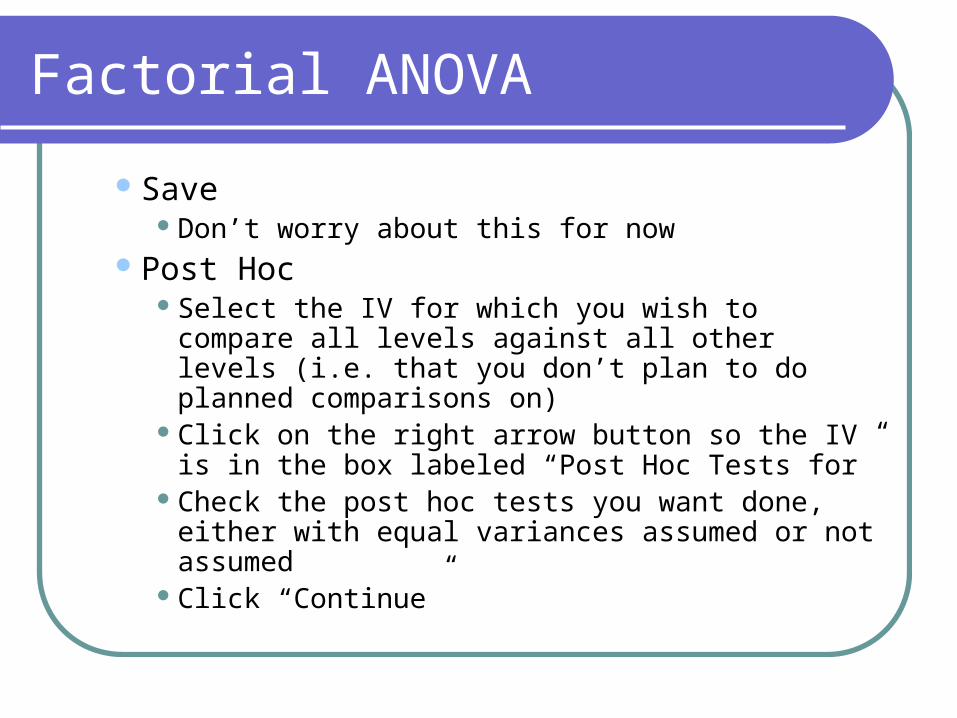
Factorial ANOVA

SaveDon’t worry about this for now

Post HocSelect the IV for which you wish to compare all

levels against all other levels (i.e. that you don’t plan to do planned comparisons on)

Click on the right arrow button so the IV is in the box labeled “Post Hoc Tests for”

Check the post hoc tests you want done, either with equal variances assumed or not assumed

Click “Continue”

Multiple Comparisons


.3021 .21779 .637 -.2969 .9010

.2587 .72939 .997 -1.7472 2.2646

-.4913 .72939 .962 -2.4972 1.5146

-.4746 .46474 .845 -1.7527 .8035

-.3021 .21779 .637 -.9010 .2969

-.0433 .75423 1.000 -2.1176 2.0309

-.7933 .75423 .831 -2.8676 1.2809

-.7767 .50282 .535 -2.1595 .6061

-.2587 .72939 .997 -2.2646 1.7472

.0433 .75423 1.000 -2.0309 2.1176

-.7500 1.02637 .949 -3.5727 2.0727

-.7333 .85873 .913 -3.0949 1.6283

.4913 .72939 .962 -1.5146 2.4972

.7933 .75423 .831 -1.2809 2.8676

.7500 1.02637 .949 -2.0727 3.5727

.0167 .85873 1.000 -2.3449 2.3783

.4746 .46474 .845 -.8035 1.7527

.7767 .50282 .535 -.6061 2.1595

.7333 .85873 .913 -1.6283 3.0949

-.0167 .85873 1.000 -2.3783 2.3449

.3021 .21779 .839 -.3137 .9179

.2587 .72939 1.000 -1.8036 2.3211

-.4913 .72939 .999 -2.5536 1.5711

-.4746 .46474 .975 -1.7887 .8394

-.3021 .21779 .839 -.9179 .3137

-.0433 .75423 1.000 -2.1759 2.0892

-.7933 .75423 .969 -2.9259 1.3392

-.7767 .50282 .733 -2.1984 .6450

-.2587 .72939 1.000 -2.3211 1.8036

.0433 .75423 1.000 -2.0892 2.1759

-.7500 1.02637 .998 -3.6521 2.1521

-.7333 .85873 .993 -3.1614 1.6947

.4913 .72939 .999 -1.5711 2.5536

.7933 .75423 .969 -1.3392 2.9259

.7500 1.02637 .998 -2.1521 3.6521

.0167 .85873 1.000 -2.4114 2.4447

.4746 .46474 .975 -.8394 1.7887

.7767 .50282 .733 -.6450 2.1984

.7333 .85873 .993 -1.6947 3.1614

-.0167 .85873 1.000 -2.4447 2.4114

(J) raceAfrican American

Asian American

Hispanic

Other

Caucasian

Asian American

Hispanic

Other

Caucasian

African American

Hispanic

Other

Caucasian

African American

Asian American

Other

Caucasian

African American

Asian American

Hispanic

African American

Asian American

Hispanic

Other

Caucasian

Asian American

Hispanic

Other

Caucasian

African American

Hispanic

Other

Caucasian

African American

Asian American

Other

Caucasian

African American

Asian American

Hispanic

(I) raceCaucasian

African American

Asian American

Hispanic

Other

Caucasian

African American

Asian American

Hispanic

Other

Tukey HSD

Sidak

MeanDifference

(I-J) Std. Error Sig. Lower Bound Upper Bound

95% Confidence Interval

Based on observed means.

genbad

25 3.7900

2 3.8333

199 4.0921

5 4.5667

2 4.5833

.809

25 3.7900

2 3.8333

199 4.0921

5 4.5667

2 4.5833

.753

raceAfrican American

Asian American

Caucasian

Other

Hispanic

Sig.

African American

Asian American

Caucasian

Other

Hispanic

Sig.

Tukey HSDa,b,c

Ryan-Einot-Gabriel-Welsch Range

c

N 1

Subset

Means for groups in homogeneous subsets are displayed.Based on Type III Sum of SquaresThe error term is Mean Square(Error) = 1.053.

Uses Harmonic Mean Sample Size = 4.016.a.

The group sizes are unequal. The harmonic mean of thegroup sizes is used. Type I error levels are not guaranteed.

b.

Alpha = .05.c.

Factorial ANOVA

PlotsHorizontal Axis

What IV is on the x-axis

Separate LinesSeparate Plots

Factorial ANOVA

The following graph has the IV “Race” on the horizontal axis and separate lines by the IV “Gender”

Factorial ANOVA

ModelAllows you to:

Denote which main effects and interactions you are interested in testing (default is to test ALL of them)

Specify which type of sum of squares to use

Usually you won’t be tinkering with this

Factorial ANOVA

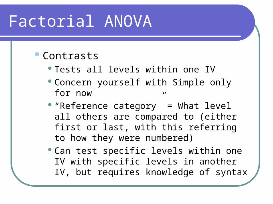
ContrastsTests all levels within one IVConcern yourself with Simple only for now “Reference category” = What level all others are

compared to (either first or last, with this referring to how they were numbered)

Can test specific levels within one IV with specific levels in another IV, but requires knowledge of syntax

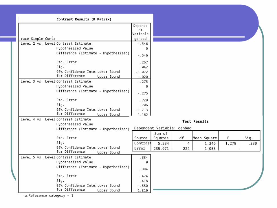
Contrast Results (K Matrix)

-.546

0

-.546

.267

.042

-1.072

-.020

-.275

0

-.275

.729

.706

-1.713

1.162

.107

0

.107

.867

.902

-1.602

1.815

.384

0

.384

.474

.418

-.550

1.319

Contrast Estimate

Hypothesized Value

Difference (Estimate - Hypothesized)

Std. Error

Sig.

Lower Bound

Upper Bound

95% Confidence Intervalfor Difference

Contrast Estimate

Hypothesized Value


Std. Error

Sig.

Lower Bound

Upper Bound


Contrast Estimate

Hypothesized Value


Std. Error

Sig.

Lower Bound

Upper Bound


Contrast Estimate

Hypothesized Value


Std. Error

Sig.

Lower Bound

Upper Bound


race Simple Contrasta

Level 2 vs. Level 1

Level 3 vs. Level 1

Level 4 vs. Level 1

Level 5 vs. Level 1

genbad

Dependent

Variable

Reference category = 1a.

Test Results


5.384 4 1.346 1.278 .280

235.971 224 1.053

SourceContrast

Error


Factorial ANOVA

Tests of Between-Subjects Effects


11.653a 8 1.457 1.383 .205

358.168 1 358.168 339.997 .000

.655 1 .655 .622 .431

6.010 4 1.502 1.426 .226

5.935 3 1.978 1.878 .134

235.971 224 1.053

4110.717 233

247.624 232

SourceCorrected Model

Intercept

gender

race

gender * race

Error

Total

Corrected Total

Type III Sumof Squares df Mean Square F Sig.

R Squared = .047 (Adjusted R Squared = .013)a.

Factorial ANOVA

Interpreting interactions See graphs

Documents

One-Way and Factorial ANOVA SPSS Lab #3. One-Way ANOVA Two ways to run a one-way ANOVA 1.Analyze Compare Means One-Way ANOVA Use if you have multiple