Analysis of Variance (ANOVA)

Cancer Research UK – 10th of May 2018

D.-L. Couturier / R. Nicholls / M. Fernandes

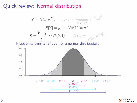
Quick review: Normal distribution

Y ∼ N(µ, σ2), fY (y) =1√2πσ2

e−(y−µ)2

2σ2

E[Y ] = µ, Var[Y ] = σ2,

Z =Y − µσ

∼ N(0, 1), fZ(z) =1√2π

e−z2

2 .

Probability density function of a normal distribution:

99.73%

µ− 3σ µ+ 3σ

95.45%

µ− 2σ µ+ 2σ

68.27%µ− σ µ+ σµ

0.0

0.1

0.2

0.3

0.4

2

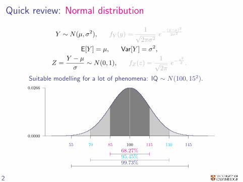
Quick review: Normal distribution

Y ∼ N(µ, σ2), fY (y) =1√2πσ2

e−(y−µ)2

2σ2

E[Y ] = µ, Var[Y ] = σ2,

Z =Y − µσ

∼ N(0, 1), fZ(z) =1√2π

e−z2

2 .

Suitable modelling for a lot of phenomena: IQ ∼ N(100, 152).

99.73%

55 145

95.45%

70 130

68.27%85 115100

0.0000

0.0266

2

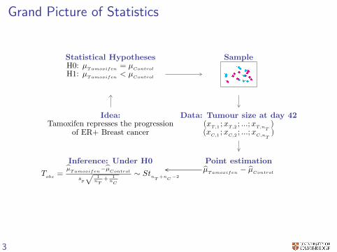
Grand Picture of Statistics

Statistical HypothesesH0: µ

Tamoxifen= µ

Control

H1: µTamoxifen

< µControl

Idea:Tamoxifen represses the progression

of ER+ Breast cancer

Sample

Data: Tumour size at day 42(x

T,1;x

T,2; ...;x

T,nT)

(xC,1

;xC,2

; ...;xC,n

T)

Point estimationµ̂

Tamoxifen− µ̂

Control

Inference: Under H0

Tobs

=µ̂Tamoxifen

−µ̂Control

sp√

1nT

+ 1nC

∼ StnT

+nC

−2

3

Grand Picture of Statistics

Statistical HypothesesH0: µ

Tamoxifen= µ

Control

H1: µTamoxifen

< µControl

Idea:Tamoxifen represses the progression

of ER+ Breast cancer

Sample

Data: Tumour size at day 42(x

T,1;x

T,2; ...;x

T,nT)

(xC,1

;xC,2

; ...;xC,n

T)

Point estimationµ̂

Tamoxifen− µ̂

Control

Inference: Under H0

Tobs

=µ̂Tamoxifen

−µ̂Control

sp√

1nT

+ 1nC

∼ StnT

+nC

−2

-4 -3 -2 -1 0 1 2 3 4

T

StnT

+nC

−2

p− value = P (T < Tobs

)

3

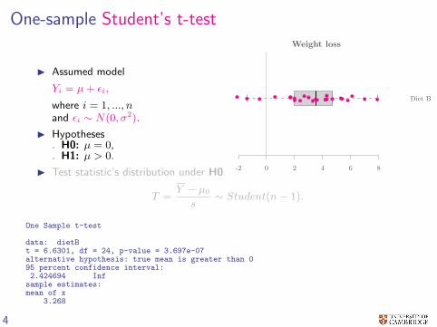
One-sample Student’s t-testWeight loss

-2 0 2 4 6 8

Diet B

I Assumed model

Yi = µ+ εi,

where i = 1, ..., nand εi ∼ N(0, σ2).

I Hypotheses. H0: µ = 0,. H1: µ > 0.

I Test statistic’s distribution under H0

T =Y − µ0

s∼ Student(n− 1).

One Sample t-test

data: dietBt = 6.6301, df = 24, p-value = 3.697e-07alternative hypothesis: true mean is greater than 095 percent confidence interval:2.424694 Infsample estimates:mean of x

3.268

4

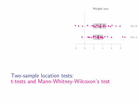
Weight loss

-2 0 2 4 6 8

Diet B

Diet A

Two-sample location tests:t-tests and Mann-Whitney-Wilcoxon’s test

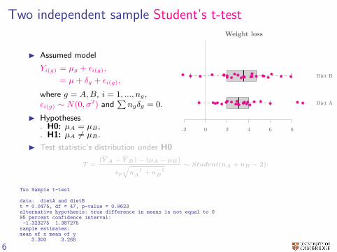
Two independent sample Student’s t-testWeight loss

-2 0 2 4 6 8

Diet B

Diet A

I Assumed model

Yi(g) = µg + εi(g),

= µ+ δg + εi(g),

where g = A,B, i = 1, ..., ng,εi(g) ∼ N(0, σ2) and

∑ngδg = 0.

I Hypotheses. H0: µA = µB ,. H1: µA 6= µB .

I Test statistic’s distribution under H0

T =(Y A − Y B)− (µA − µB)

sp

√n−1A + n−1

B

∼ Student(nA + nB − 2).

Two Sample t-test

data: dietA and dietBt = 0.0475, df = 47, p-value = 0.9623alternative hypothesis: true difference in means is not equal to 095 percent confidence interval:-1.323275 1.387275sample estimates:mean of x mean of y

3.300 3.268

6

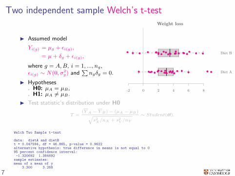
Two independent sample Welch’s t-testWeight loss

-2 0 2 4 6 8

Diet B

Diet A

I Assumed model

Yi(g) = µg + εi(g),

= µ+ δg + εi(g),

where g = A,B, i = 1, ..., ng,εi(g) ∼ N(0, σ2

g) and∑ngδg = 0.

I Hypotheses. H0: µA = µB ,. H1: µA 6= µB .

I Test statistic’s distribution under H0

T =(Y A − Y B)− (µA − µB)√

s2X/nX + s2Y /nY

∼ Student(df).

Welch Two Sample t-test

data: dietA and dietBt = 0.047594, df = 46.865, p-value = 0.9622alternative hypothesis: true difference in means is not equal to 095 percent confidence interval:-1.320692 1.384692sample estimates:mean of x mean of y

3.300 3.268

7

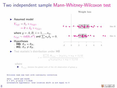
Two independent sample Mann-Whitney-Wilcoxon testWeight loss

-2 0 2 4 6 8

Diet B

Diet A

I Assumed model

Yi(g) = θg + εi(g),

= θ + δg + εi(g),

where g = A,B, i = 1, ..., ng,εi(g) ∼ iid(0, σ2) and

∑ngδg = 0.

I Hypotheses. H0: θA = θB ,. H1: θA 6= θB .

I Test statistic’s distribution under H0

z =

∑nBi=1 Ri(g) − [nB(nA + nB + 1)/2]√

nAnB(nA + nB + 1)/12,

whereI Ri(g) denotes the global rank of the ith observation of group g.

Wilcoxon rank sum test with continuity correction

data: dietA and dietBW = 277, p-value = 0.6526alternative hypothesis: true location shift is not equal to 0

8

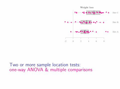
Weight loss

-2 0 2 4 6 8

Diet B

Diet A

Diet C

Two or more sample location tests:one-way ANOVA & multiple comparisons

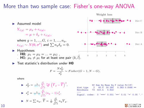
More than two sample case: Fisher’s one-way ANOVAWeight loss

-2 0 2 4 6 8

Diet B

Diet A

Diet C

I Assumed model

Yi(g) = µg + εi(g),

= µ+ δg + εi(g),

where g = 1, ..., G, i = 1, ..., ng,εi(g) ∼ N(0, σ2) and

∑ngδg = 0.

I Hypotheses. H0: µ1 = µ2 = ... = µG ,. H1: µk 6= µl for at least one pair (k, l).

I Test statistic’s distribution under H0

F =Ns2

Y

s2p∼ Fisher(G− 1, N −G),

where

I s2Y

= 1G−1

G∑g=1

ngN

(Y g − Y

)2,

I s2p = 1N−G

G∑g=1

(ng − 1)s2g ,

I N =∑ng, Y = 1

N

G∑g=1

ngY g .

Df Sum Sq Mean Sq F value Pr(>F)diet.type 2 60.5 30.264 5.383 0.0066 **Residuals 73 410.4 5.622---Signif. codes: 0 ‘***’ 0.001 ‘**’ 0.01 ‘*’ 0.05 ‘.’ 0.1 ‘ ’ 1

10

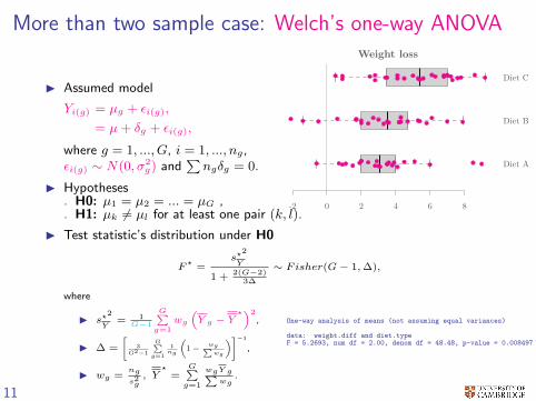
More than two sample case: Welch’s one-way ANOVAWeight loss

-2 0 2 4 6 8

Diet B

Diet A

Diet C

I Assumed model

Yi(g) = µg + εi(g),

= µ+ δg + εi(g),

where g = 1, ..., G, i = 1, ..., ng,εi(g) ∼ N(0, σ2

g) and∑ngδg = 0.

I Hypotheses. H0: µ1 = µ2 = ... = µG ,. H1: µk 6= µl for at least one pair (k, l).

I Test statistic’s distribution under H0

F?

=s?

2

Y

1 +2(G−2)

3∆

∼ Fisher(G− 1,∆),

where

I s?2

Y= 1

G−1

G∑g=1

wg(Y g − Y

?)2,

I ∆ =

[3

G2−1

G∑g=1

1ng

(1− wg∑

wg

)]−1

,

I wg =ng

s2g, Y

?=

G∑g=1

wgY g∑wg

.

One-way analysis of means (not assuming equal variances)

data: weight.diff and diet.typeF = 5.2693, num df = 2.00, denom df = 48.48, p-value = 0.008497

11

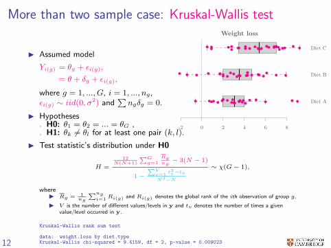
More than two sample case: Kruskal-Wallis testWeight loss

-2 0 2 4 6 8

Diet B

Diet A

Diet C

I Assumed model

Yi(g) = θg + εi(g),

= θ + δg + εi(g),

where g = 1, ..., G, i = 1, ..., ng,εi(g) ∼ iid(0, σ2) and

∑ngδg = 0.

I Hypotheses. H0: θ1 = θ2 = ... = θG ,. H1: θk 6= θl for at least one pair (k, l).

I Test statistic’s distribution under H0

H =

12N(N+1)

∑Gg=1

Rgng− 3(N − 1)

1−∑Vv=1

t3v−tvN3−N

∼ χ(G− 1),

whereI Rg = 1

ng

∑ngi=1

Ri(g) and Ri(g) denotes the global rank of the ith observation of group g,

I V is the number of different values/levels in y and tv denotes the number of times a givenvalue/level occurred in y.

Kruskal-Wallis rank sum test

data: weight.loss by diet.typeKruskal-Wallis chi-squared = 9.4159, df = 2, p-value = 0.00902312

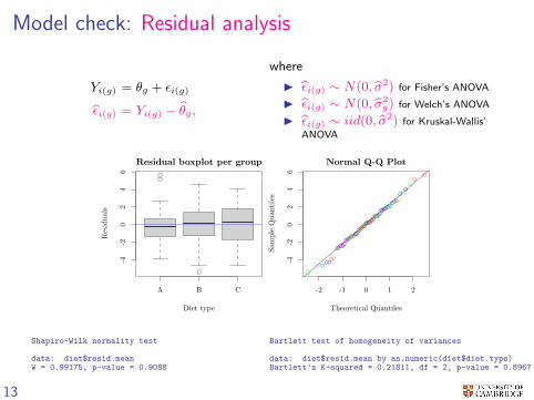
Model check: Residual analysis

Yi(g) = θg + εi(g)

ε̂i(g) = Yi(g) − θ̂g,

where

I ε̂i(g) ∼ N(0, σ̂2) for Fisher’s ANOVA

I ε̂i(g) ∼ N(0, σ̂2g) for Welch’s ANOVA

I ε̂i(g) ∼ iid(0, σ̂2) for Kruskal-Wallis’

ANOVA

A B C

-4-2

02

46

Residual boxplot per group

Diet type

Residuals

-2 -1 0 1 2-4

-20

24

6

Normal Q-Q Plot

Theoretical Quantiles

Sam

ple

Quan

tiles

Shapiro-Wilk normality test

data: diet$resid.meanW = 0.99175, p-value = 0.9088

Bartlett test of homogeneity of variances

data: diet$resid.mean by as.numeric(diet$diet.type)Bartlett’s K-squared = 0.21811, df = 2, p-value = 0.8967

13

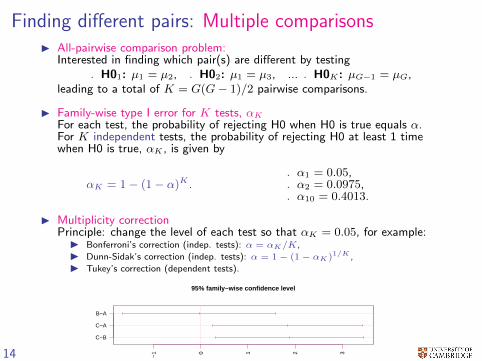
Finding different pairs: Multiple comparisonsI All-pairwise comparison problem:

Interested in finding which pair(s) are different by testing. H01: µ1 = µ2, . H02: µ1 = µ3, ... . H0K : µG−1 = µG,

leading to a total of K = G(G− 1)/2 pairwise comparisons.

I Family-wise type I error for K tests, αK

For each test, the probability of rejecting H0 when H0 is true equals α.For K independent tests, the probability of rejecting H0 at least 1 timewhen H0 is true, αK , is given by

αK = 1− (1− α)K .. α1 = 0.05,. α2 = 0.0975,. α10 = 0.4013.

I Multiplicity correctionPrinciple: change the level of each test so that αK = 0.05, for example:

I Bonferroni’s correction (indep. tests): α = αK/K,

I Dunn-Sidak’s correction (indep. tests): α = 1− (1− αK)1/K ,

I Tukey’s correction (dependent tests).

−1 0 1 2 3

C−B

C−A

B−A

95% family−wise confidence level

Differences in mean levels of diet.type

14

Weight loss

-2 0 2 4 6 8

Diet A

Diet B

Diet C

Diet A

Diet B

Diet C

Male

Fem

ale

Two or more sample location tests:two-way ANOVA

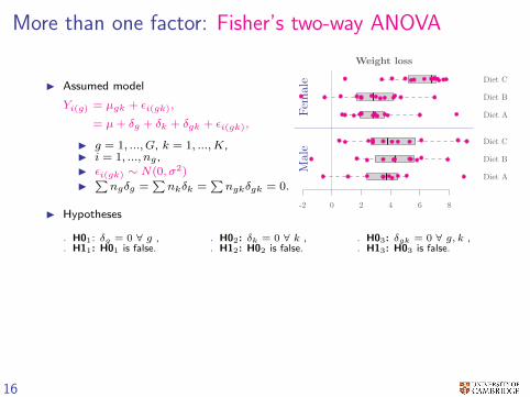
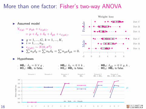
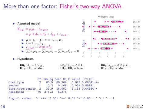
More than one factor: Fisher’s two-way ANOVA

Weight loss

-2 0 2 4 6 8

Diet A

Diet B

Diet C

Diet A

Diet B

Diet C

Male

Fem

aleI Assumed model

Yi(g) = µgk + εi(gk),

= µ+ δg + δk + δgk + εi(gk),

I g = 1, ..., G, k = 1, ...,K,I i = 1, ..., ng ,I εi(gk) ∼ N(0, σ2)

I∑ngδg =

∑nkδk =

∑ngkδgk = 0.

I Hypotheses

. H01: δg = 0 ∀ g ,

. H11: H01 is false.. H02: δk = 0 ∀ k ,. H12: H02 is false.

. H03: δgk = 0 ∀ g, k ,

. H13: H03 is false.

16

More than one factor: Fisher’s two-way ANOVA

Weight loss

-2 0 2 4 6 8

Diet A

Diet B

Diet C

Diet A

Diet B

Diet C

Male

Fem

aleI Assumed model

Yi(g) = µgk + εi(gk),

= µ+ δg + δk + δgk + εi(gk),

I g = 1, ..., G, k = 1, ...,K,I i = 1, ..., ng ,I εi(gk) ∼ N(0, σ2)

I∑ngδg =

∑nkδk =

∑ngkδgk = 0.

I Hypotheses

. H01: δg = 0 ∀ g ,

. H11: H01 is false.. H02: δk = 0 ∀ k ,. H12: H02 is false.

. H03: δgk = 0 ∀ g, k ,

. H13: H03 is false.

0.0

0.5

1.0

1.5

2.0

2.5

3.0

Meanweigh

tloss

µ

A B C

Scenario 1

A B C

Scenario 2

A B C

H11

Scenario 3

A B C

H12

Scenario 4

A B C

H11 & H12

Scenario 5

A B C

H11 & H12 & H13

Scenario 6

Male Female

16

More than one factor: Fisher’s two-way ANOVA

Weight loss

-2 0 2 4 6 8

Diet A

Diet B

Diet C

Diet A

Diet B

Diet C

Male

Fem

aleI Assumed model

Yi(g) = µgk + εi(gk),

= µ+ δg + δk + δgk + εi(gk),

I g = 1, ..., G, k = 1, ...,K,I i = 1, ..., ng ,I εi(gk) ∼ N(0, σ2)

I∑ngδg =

∑nkδk =

∑ngkδgk = 0.

I Hypotheses

. H01: δg = 0 ∀ g ,

. H11: H01 is false.. H02: δk = 0 ∀ k ,. H12: H02 is false.

. H03: δgk = 0 ∀ g, k ,

. H13: H03 is false.

Df Sum Sq Mean Sq F value Pr(>F)diet.type 2 60.5 30.264 5.629 0.00541 **gender 1 0.2 0.169 0.031 0.85991diet.type:gender 2 33.9 16.952 3.153 0.04884 *Residuals 70 376.3 5.376---Signif. codes: 0 ‘***’ 0.001 ‘**’ 0.01 ‘*’ 0.05 ‘.’ 0.1 ‘ ’ 1

16

Summary

17