Local Search - Politechnika Pozna„ska

DM811HEURISTICS AND LOCAL SEARCH ALGORITHMS

FOR COMBINATORIAL OPTIMZATION

Lecture 7

Local Search

Marco Chiarandini

slides in part based onhttp://www.sls-book.net/H. Hoos and T. Stützle, 2005

Outline

1. Local Search, Basic ElementsComponents and AlgorithmsBeyond Local OptimaComputational Complexity

2. Fundamental Search Space PropertiesIntroductionNeighborhood RepresentationsDistancesLandscape CharacteristicsFitness-Distance CorrelationRuggednessPlateauxBarriers and Basins

3. Efficient Local SearchEfficiency vs EffectivenessApplication Examples

Traveling Salesman ProblemSingle Machine Total Weighted Tardiness ProblemGraph Coloring

2

Outline





3

Definition: Local Search Algorithm

For given problem instance π:

1. search space S(π) (solution set S ′(π) ⊆ S(π))

2. neighborhood function N (π) : S(π) 7→ 2S(π)

3. evaluation function f(π) : S 7→ R

4. set of memory states M(π)

5. initialization function init : ∅ 7→ P(S(π)×M(π))

6. step function step : S(π)×M(π) 7→ P(S(π)×M(π))

7. termination predicate terminate : S(π)×M(π) 7→ P({>,⊥})

5

Example: Uninformed random walk for SAT (1)

I search space S: set of all truth assignments to variablesin given formula F(solution set S ′: set of all models of F)

I neighborhood function N : 1-flip neighborhood, i.e., assignments areneighbors under N iff they differ inthe truth value of exactly one variable

I evaluation function not used, or f(s) = 0 if model f(s) = 1 otherwise

I memory: not used, i.e., M := {0}

6

Example: Uninformed random walk for SAT (continued)

I initialization: uniform random choice from S, i.e.,init(, {a ′,m}) := 1/|S| for all assignments a ′ andmemory states m

I step function: uniform random choice from current neighborhood, i.e.,step({a,m}, {a ′,m}) := 1/|N(a)|for all assignments a and memory states m,where N(a) := {a ′ ∈ S | N (a, a ′)} is the set ofall neighbors of a.

I termination: when model is found, i.e.,terminate({a,m}, {>}) := 1 if a is a model of F, and 0 otherwise.

7

Definition: LS Algorithm Components (continued)

Search SpaceDefined by the solution representation:

I permutationsI linear (scheduling)I circular (TSP)

I arrays (assignment problems: GCP)

I sets or lists (partition problems: Knapsack)

8


Neighborhood function N (π) : S(π) 7→ 2S(π)

Also defined as: N : S× S→ {T, F} or N ⊆ S× S

I neighborhood (set) of candidate solution s: N(s) := {s ′ ∈ S | N (s, s ′)}

I neighborhood size is |N(s)|

I neighborhood is symmetric if: s ′ ∈ N(s)⇒ s ∈ N(s ′)

I neighborhood graph of (S,N, π) is a directed vertex-weighted graph:GN (π) := (V,A) with V = S(π) and (uv) ∈ A⇔ v ∈ N(u)(if symmetric neighborhood ⇒ undirected graph)

Note on notation: N when set, N when collection of sets or function

9

A neighborhood function is also defined by means of an operator.

An operator ∆ is a collection of operator functions δ : S→ S such that

s ′ ∈ N(s) ⇐⇒ ∃ δ ∈ ∆, δ(s) = s ′

Definitionk-exchange neighborhood: candidate solutions s, s ′ are neighbors iff s differsfrom s ′ in at most k solution components

Examples:

I 1-exchange (flip) neighborhood for SAT(solution components = single variable assignments)

I 2-exchange neighborhood for TSP(solution components = edges in given graph)

10


Note:

I Local search implements a walk through the neighborhood graph

I Procedural versions of init, step and terminate implement samplingfrom respective probability distributions.

I Memory state m can consist of multiple independent attributes, i.e.,M(π) := M1 ×M2 × . . .×Ml(π).

I Local search algorithms are Markov processes:behavior in any search state {s,m} depends onlyon current position s and (limited) memory m.

11


Search step (or move):pair of search positions s, s ′ for whichs ′ can be reached from s in one step, i.e., N (s, s ′) andstep({s,m}, {s ′,m ′}) > 0 for some memory states m,m ′ ∈M.

I Search trajectory: finite sequence of search positions < s0, s1, . . . , sk >such that (si−1, si) is a search step for any i ∈ {1, . . . , k}

and the probability of initializing the search at s0is greater zero, i.e., init({s0,m}) > 0 for some memory state m ∈M.

I Search strategy: specified by init and step function;to some extent independent of problem instance andother components of LS algorithm.

I randomI based on evaluation functionI based on memory

12

Uninformed Random PickingI N := S× SI does not use memory and evaluation functionI init, step: uniform random choice from S,

i.e., for all s, s ′ ∈ S, init(s) := step({s}, {s ′}) := 1/|S|

Uninformed Random WalkI does not use memory and evaluation functionI init: uniform random choice from S

I step: uniform random choice from current neighborhood,

i.e., for all s, s ′ ∈ S, step({s}, {s ′}) :=

{1/|N(s)| if s ′ ∈ N(s)

0 otherwise

Note: These uninformed LS strategies are quite ineffective,but play a role in combination with more directed search strategies.

13


Evaluation (or cost) function:I function f(π) : S(π) 7→ R that maps candidate solutions of

a given problem instance π onto real numbers,such that global optima correspond to solutions of π;

I used for ranking or assessing neighbors of currentsearch position to provide guidance to search process.

Evaluation vs objective functions:I Evaluation function: part of LS algorithm.I Objective function: integral part of optimization problem.I Some LS methods use evaluation functions different from given objective

function (e.g., dynamic local search).

14

Iterative ImprovementI does not use memoryI init: uniform random choice from S

I step: uniform random choice from improving neighbors,i.e., step({s}, {s ′}) := 1/|I(s)| if s ′ ∈ I(s), and 0 otherwise,where I(s) := {s ′ ∈ S | N (s, s ′) and f(s ′) < f(s)}

I terminates when no improving neighbor available(to be revisited later)

I different variants through modifications of step function(to be revisited later)

Note: II is also known as iterative descent or hill-climbing.

15

Example: Iterative Improvement for SAT

I search space S: set of all truth assignments to variablesin given formula F(solution set S ′: set of all models of F)

I neighborhood function N : 1-flip neighborhood(as in Uninformed Random Walk for SAT)


I initialization: uniform random choice from S, i.e., init(∅, {a ′}) := 1/|S|

for all assignments a ′

I evaluation function: f(a) := number of clauses in Fthat are unsatisfied under assignment a(Note: f(a) = 0 iff a is a model of F.)

I step function: uniform random choice from improving neighbors, i.e.,step(a, a ′) := 1/#I(a) if s ′ ∈ I(a),and 0 otherwise, where I(a) := {a ′ | N (a, a ′) ∧ f(a ′) < f(a)}

I termination: when no improving neighbor is availablei.e., terminate(a,>) := 1 if I(a) = ∅, and 0 otherwise.

16

Definition:

I Local minimum: search position without improving neighbors w.r.t.given evaluation function f and neighborhood N ,i.e., position s ∈ S such that f(s) ≤ f(s ′) for all s ′ ∈ N(s).

I Strict local minimum: search position s ∈ S such thatf(s) < f(s ′) for all s ′ ∈ N(s).

I Local maxima and strict local maxima: defined analogously.

17

There might be more than one neighbor that have better cost.

Pivoting rule decides which to choose:

I Best Improvement (aka gradient descent, steepest descent, greedyhill-climbing): Choose maximally improving neighbor,i.e., randomly select from I∗(s) := {s ′ ∈ N(s) | f(s ′) = f∗},where f∗ := min{f(s ′) | s ′ ∈ N(s)}.

Note: Requires evaluation of all neighbors in each step.

I First Improvement: Evaluate neighbors in fixed order,choose first improving step encountered.

Note: Can be much more efficient than Best Improvement; order ofevaluation can have significant impact on performance.

18

Example: Iterative Improvement for TSP (2-opt)

procedure TSP-2opt-first(s)input: an initial candidate tour s ∈ S(∈)

output: a local optimum s ∈ S(π)

∆ = 0;do

Improvement=FALSE;for i = 1 to n− 2 doif i = 1 then n ′ = n− 1 elsen ′ = n

for j = i+ 2 to n ′ do∆ij = d(ci, cj) + d(ci+1, cj+1) − d(ci, ci+1) − d(cj, cj+1)

if ∆ij < 0 thenUpdateTour(s,i,j);Improvement=TRUE;

endend

until Improvement==FALSE;end TSP-2opt-first

19

Example: Random order first improvement for the TSP

I Given: TSP instance G with vertices v1, v2, . . . , vn.I search space: Hamiltonian cycles in G;

use standard 2-exchange neighborhood

I Initialization:I search position := fixed canonical path < v1, v2, . . . , vn, v1 >I P := random permutation of {1, 2, . . . , n}

I Search steps: determined using first improvementw.r.t. f(p) = weight of path p,evaluating neighbors in order of P (does not change throughout search)

I Termination: when no improving search step possible(local minimum)

20

Example: Random order first improvement for SAT

procedure URW-for-SAT(F,maxSteps)input: propositional formula F, integer maxStepsoutput: model of F or ∅choose assignment ϕ of truth values to all variables in F

uniformly at random;steps := 0;while not((ϕ satisfies F) and (steps < maxSteps)) do

select x uniformly at random from {x ′|x ′ is a variable in F andchanging value of x ′ in ϕ decreases the number of unsatisfied clauses};steps := steps+1;

endif ϕ satisfies F then

return ϕelse

return ∅end

end URW-for-SAT

21

A note on terminology

Heuristic Methods ≡ Metaheuristics ≡ Local Search Methods ≡ StochasticLocal Search Methods ≡ Hybrid Metaheuristics

Method 6= Algorithm

Stochastic Local Search (SLS) algorithms allude to:I Local Search: informed search based on local or incomplete knowledge

as opposed to systematic searchI Stochastic: use randomized choices in generating and modifying

candidate solutions. They are introduced whenever it is unknown whichdeterministic rules are profitable for all the instances of interest.

22

Simple Mechanisms for Escaping from Local Optima

I Enlarge the neighborhood

I Restart: re-initialize search whenever a local optimumis encountered.(Often rather ineffective due to cost of initialization.)

I Non-improving steps: in local optima, allow selection ofcandidate solutions with equal or worse evaluation function value, e.g.,using minimally worsening steps.(Can lead to long walks in plateaus, i.e., regions ofsearch positions with identical evaluation function.)

Note: None of these mechanisms is guaranteed to alwaysescape effectively from local optima.

24

Diversification vs Intensification

I Goal-directed and randomized components of LS strategy need to bebalanced carefully.

I Intensification: aims to greedily increase solution quality or probability,e.g., by exploiting the evaluation function.

I Diversification: aim to prevent search stagnation by preventing searchprocess from getting trapped in confined regions.

Examples:I Iterative Improvement (II): intensification strategy.I Uninformed Random Walk/Picking (URW/P): diversification strategy.

Balanced combination of intensification and diversification mechanisms formsthe basis for advanced LS methods.

25

Computational Complexity of Local Search (1)

For a local search algorithm to be effective, search initializationand individual search steps should be efficiently computable.

Complexity class PLS: class of problems for which a localsearch algorithm exists with polynomial time complexity for:

I search initializationI any single search step, including computation of

any evaluation function value

For any problem in PLS . . .I local optimality can be verified in polynomial timeI improving search steps can be computed in polynomial timeI but: finding local optima may require super-polynomial time

27

Computational Complexity of Local Search (2)

PLS-complete: Among the most difficult problems in PLS;if for any of these problems local optima can be foundin polynomial time, the same would hold for all problems in PLS.

Some complexity results:I TSP with k-exchange neighborhood with k > 3

is PLS-complete.

I TSP with 2- or 3-exchange neighborhood is in PLS, butPLS-completeness is unknown.

28

Outline





29

Learning goals of this section

I Review basic theoretical concepts

I Learn about techniques and goals of experimental search space analysis.

I Develop intuition on which features of local search are adequate tocontrast a specific situation.

31

Definitions

I Search space S

I Neighborhood function N : S ⊆ 2S

I Evaluation function f(π) : S 7→ R

I Problem instance π

Definition:The search landscape L is the vertex-labeled neighborhood graph given bythe triplet L = (S(π), N(π), f(π)).

32

Ideal visualization of metaheuristic principles

I Simplified landscaperepresentation I Tabu Search I Guided Local Search

I Iterated Local Search I Evolutionary Alg.

33

Fundamental Search Space Properties

The behavior and performance of an LS algorithm on a given probleminstance crucially depends on properties of the respective search space.

Simple properties of search space S:I search space size |S|

I reachability: solution j is reachable from solution i if neighborhoodgraph has a path from i to j.

I strongly connected neighborhood graph

I weakly optimally connected neighborhood graph

I search space diameter diam(GN )(= maximal distance between any two candidate solutions)Note: Diameter of GN = worst-case lower bound for number of searchsteps required for reaching (optimal) solutions.Maximal shortest path between any two vertices in the neighborhoodgraph.

34

Solution Representations and Neighborhoods

Three different types of solution representations:I Permutation

I linear permutation: Single Machine Total Weighted Tardiness ProblemI circular permutation: Traveling Salesman Problem

I Assignment: Graph Coloring Problem, SAT, CSPI Set, Partition: Knapsack, Max Independent Set

A neighborhood function N : S→ S× S is also defined through an operator.An operator ∆ is a collection of operator functions δ : S→ S such that

s ′ ∈ N(s) ⇐⇒ ∃δ ∈ ∆ | δ(s) = s ′

36

Permutations

Π(n) indicates the set all permutations of the numbers {1, 2, . . . , n}

(1, 2 . . . , n) is the identity permutation ι.

If π ∈ Π(n) and 1 ≤ i ≤ n then:I πi is the element at position iI posπ(i) is the position of element i

Alternatively, a permutation is a bijective function π(i) = πi

the permutation product π · π ′ is the composition (π · π ′)i = π ′(π(i))

For each π there exists a permutation such that π−1 · π = ι

∆N ⊂ Π

37

Neighborhood Operators for Linear Permutations

Swap operator∆S = {δiS|1 ≤ i ≤ n}

δiS(π1 . . . πiπi+1 . . . πn) = (π1 . . . πi+1πi . . . πn)

Interchange operator∆X = {δ

ijX |1 ≤ i < j ≤ n}

δijX(π) = (π1 . . . πi−1πjπi+1 . . . πj−1πiπj+1 . . . πn)

(≡ set of all transpositions)

Insert operator∆I = {δ

ijI |1 ≤ i ≤ n, 1 ≤ j ≤ n, j 6= i}

δijI (π) =

{(π1 . . . πi−1πi+1 . . . πjπiπj+1 . . . πn) i < j

(π1 . . . πjπiπj+1 . . . πi−1πi+1 . . . πn) i > j

38

Neighborhood Operators for Circular Permutations

Reversal (2-edge-exchange)

∆R = {δijR |1 ≤ i < j ≤ n}

δijR (π) = (π1 . . . πi−1πj . . . πiπj+1 . . . πn)

Block moves (3-edge-exchange)

∆B = {δijkB |1 ≤ i < j < k ≤ n}

δijB (π) = (π1 . . . πi−1πj . . . πkπi . . . πj−1πk+1 . . . πn)

Short block move (Or-edge-exchange)

∆SB = {δijSB|1 ≤ i < j ≤ n}

δijSB(π) = (π1 . . . πi−1πjπj+1πj+2πi . . . πj−1πj+3 . . . πn)

39

Neighborhood Operators for Assignments

An assignment can be represented as a mappingσ : {X1 . . . Xn}→ {v : v ∈ D, |D| = k}:

σ = {Xi = vi, Xj = vj, . . .}

One-exchange operator

∆1E = {δil1E|1 ≤ i ≤ n, 1 ≤ l ≤ k}

δil1E(σ) =

{σ : σ ′(Xi) = vl and σ ′(Xj) = σ(Xj) ∀j 6= i

}Two-exchange operator

∆2E = {δij2E|1 ≤ i < j ≤ n}

δij2E

{σ : σ ′(Xi) = σ(Xj), σ

′(Xj) = σ(Xi) and σ ′(Xl) = σ(Xl) ∀l 6= i, j}

40

Neighborhood Operators for Partitions or Sets

An assignment can be represented as a partition of objects selected and notselected s : {X}→ {C,C}

(it can also be represented by a bit string)

One-addition operator∆1E = {δv1E|v ∈ C}

δv1E(s) =

{s : C ′ = C ∪ v and C

′= C \ v}

One-deletion operator∆1E = {δv1E|v ∈ C}

δv1E(s) =

{s : C ′ = C \ v and C

′= C ∪ v}

Swap operator∆1E = {δv1E|v ∈ C,u ∈ C}

δv1E(s) =

{s : C ′ = C ∪ u \ v and C

′= C ∪ v \ u}

41

Distances

Set of paths in GN with s, s ′ ∈ S:

Φ(s, s ′) = {(s1, . . . , sh)|s1 = s, sh = s ′ ∀i : 1 ≤ i ≤ h− 1, 〈si, si+1〉 ∈ EN}

If φ = (s1, . . . , sh) ∈ Φ(s, s ′) let |φ| = h be the length of the path; then thedistance between any two solutions s, s ′ is the length of shortest pathbetween s and s ′ in GN :

dN (s, s ′) = minφ∈Φ(s,s ′)

|Φ|

diam(GN ) = max{dN (s, s ′) | s, s ′ ∈ S}

Note: with permutations it is easy to see that:

dN (π, π ′) = dN (π−1 · π ′, ι)

43

Distances for Linear Permutation Representations

I Swap neighborhood operatorcomputable in O(n2) by the precedence based distance metric:dS(π, π

′) = #{〈i, j〉|1 ≤ i < j ≤ n, posπ ′(πj) < posπ ′(πi)}.diam(GN ) = n(n− 1)/2

I Interchange neighborhood operatorComputable in O(n) +O(n) sincedX(π, π ′) = dX(π−1 · π ′, ι) = n− c(π−1 · π ′)where c(π) is the number of disjoint cycles that decompose apermutation.diam(GNX

) = n− 1

I Insert neighborhood operatorComputable in O(n) +O(n log(n)) sincedI(π, π

′) = dI(π−1 · π ′, ι) = n− |lis(π−1 · π ′)| where lis(π) denotes

the length of the longest increasing subsequence.diam(GNI

) = n− 1

44

Distances for Circular Permutation Representations

I Reversal neighborhood operatorsorting by reversal is known to be NP-hardsurrogate in TSP: bond distance

I Block moves neighborhood operatorunknown whether it is NP-hard but there does not exist a provedpolynomial-time algorithm

45

Distances for Assignment Representations

I Hamming Distance

I An assignment can be seen as a partition of n in k mutually exclusivenon-empty subsets

One-exchange neighborhood operatorThe partition-distance d1E(P,P ′) between two partitions P and P ′ isthe minimum number of elements that must be moved between subsetsin P so that the resulting partition equals P ′.The partition-distance can be computed in polynomial time by solvingan assignment problem. Given the assignment matrix M where in eachcell (i, j) it is |Si ∩ S ′j | with Si ∈ P and S ′j ∈ P ′ and defined A(P,P ′)the assignment of maximal sum then it is d1E(P,P ′) = n−A(P,P ′)

46

Example: Search space size and diameter for the TSP

I Search space size = (n− 1)!/2

I Insert neighborhoodsize = (n− 3)ndiameter = n− 2

I 2-exchange neighborhoodsize =

(n2

)= n · (n− 1)/2

diameter in [n/2, n− 2]

I 3-exchange neighborhoodsize =

(n3

)= n · (n− 1) · (n− 2)/6

diameter in [n/3, n− 1]

47

Example: Search space size and diameter for SAT

SAT instance with n variables, 1-flip neighborhood:GN = n-dimensional hypercube; diameter of GN = n.

48

Let N1 and N2 be two different neighborhood functions for the sameinstance (S, f, π) of a combinatorial optimization problem.If for all solutions s ∈ S we have N1(s) ⊆ N2(s ′) then we say that N2dominates N1

Example:In TSP, 1-insert is domnated by 3-exchange.(1-insert corresponds to 3-exchange and there are 3-exchnages that are not1-insert)

49

Other Search Space Properties

I number of (optimal) solutions |S ′|, solution density |S ′|/|S|

I distribution of solutions within the neighborhood graph

Solution densities and distributions can generally be determined by:

I exhaustive enumeration;I sampling methods;I counting algorithms (often variants of complete algorithms).

51

Example: Correlation between solution density and search costfor GWSAT over set of hard Random-3-SAT instances:

106

105

104

103

102

20 22 24 26 28 30 320

0.2

0.4

0.6

0.8

1

-log10(solution density)

sear

ch c

ost [

mea

n #

step

s]

20 22 24 26 28 30 32

-log10(solution density)

P

cdfemp. pdf (�10)

logN[26.5, 1.26]

52

Phase Transition for 3-SAT

Random instances ⇒ m clauses of n uniformly chosen variables

0

0.2

0.4

0.6

0.8

1

3 3.5 4 4.5 5 5.5 6

#cl/#var

P(s

at),

P(u

nsat

)

−4

−3

−2

−1

0

1

P(sat)P(unsat)

kcnfs mean sc (all)

log

mea

n se

arch

cos

t [C

PU

sec

]

0

0.2

0.4

0.6

0.8

1

3 3.5 4 4.5 5 5.5 6

#cl/#var

P(s

at),

P(u

nsat

)

−4

−3

−2

−1

0

1

kcnfs mean sc (unsat)kcnfs mean sc (all)nov+ mean sc (sat)

P(sat)P(unsat)

log

mea

n se

arch

cos

t [C

PU

sec

]

53

Classification of search positions

SLMIN

SLOPELEDGE

LMAXSLMAX

LMIN

IPLAT

position type > = <

SLMIN (strict local min) + – –LMIN (local min) + + –IPLAT (interior plateau) – + –SLOPE + – +LEDGE + + +LMAX (local max) – + +SLMAX (strict local max) – – +

“+” = present, “–” absent; table entries refer to neighbors withlarger (“>”) , equal (“=”), and smaller (“<”) evaluation function values

54

Example: Complete distribution of position typesfor hard Random-3-SAT instances

instance avg sc SLMIN LMIN IPLATuf20-91/easy 13.05 0% 0.11% 0%uf20-91/medium 83.25 < 0.01% 0.13% 0%uf20-91/hard 563.94 < 0.01% 0.16% 0%

instance SLOPE LEDGE LMAX SLMAXuf20-91/easy 0.59% 99.27% 0.04% < 0.01%uf20-91/medium 0.31% 99.40% 0.06% < 0.01%uf20-91/hard 0.56% 99.23% 0.05% < 0.01%

(based on exhaustive enumeration of search space;sc refers to search cost for GWSAT)

55

Example: Sampled distribution of position typesfor hard Random-3-SAT instances

instance avg sc SLMIN LMIN IPLATuf50-218/medium 615.25 0% 47.29% 0%uf100-430/medium 3 410.45 0% 43.89% 0%uf150-645/medium 10 231.89 0% 41.95% 0%

instance SLOPE LEDGE LMAX SLMAXuf50-218/medium < 0.01% 52.71% 0% 0%uf100-430/medium 0% 56.11% 0% 0%uf150-645/medium 0% 58.05% 0% 0%

(based on sampling along GWSAT trajectories;sc refers to search cost for GWSAT)

56

Local Minima

Note: Local minima impede local search progress.

Simple properties of local minima:

I number of local minima: |lmin|, local minima density |lmin|/|S|

I localization of local minima: distribution of local minima within theneighborhood graph

Problem: Determining these measures typically requiresexhaustive enumeration of search space.

⇒ Approximation based on sampling or estimation fromother measures (such as autocorrelation measures, see below).

57

Example: Distribution of local minima for the TSP

Goal: Empirical analysis of distribution of local minima forEuclidean TSP instances.

Experimental approach:

I Sample sets of local optima of three TSPLIB instances using multipleindependent runs of two TSP algorithms (3-opt, ILS).

I Measure pairwise distances between local minima (using bond distance= number of edges in which two given tours differ).

I Sample set of purportedly globally optimal tours using multipleindependent runs of high-performance TSP algorithm.

I Measure minimal pairwise distances between local minima and respectiveclosest optimal tour (using bond distance).

58

Empirical results:

Instance avg sq [%] avg dlmin avg dopt

Results for 3-optrat783 3.45 197.8 185.9pr1002 3.58 242.0 208.6pcb1173 4.81 274.6 246.0

Results for ILS algorithmrat783 0.92 142.2 123.1pr1002 0.85 177.2 143.2pcb1173 1.05 177.4 151.8

(based on local minima collected from 1 000/200 runs of 3-opt/ILS)avg sq [%]: average solution quality expressed in percentage deviation from optimalsolution

59

Interpretation:I Average distance between local minima is small compared to maximal

possible bond distance, n.⇒ Local minima are concentrated in a relatively small region of thesearch space.

I Average distance between local minima is slightly larger than distance toclosest global optimum.⇒ Optimal solutions are located centrally in region of high local minimadensity.

I Higher-quality local minima found by ILS tend to be closer to each otherand the closest global optima compared to those determined by 3-opt.⇒ Higher-quality local minima tend to be concentrated in smallerregions of the search space.

Note: These results are fairly typical for many types of TSP instances andinstances of other combinatorial problems.In many cases, local optima tend to be clustered; this is reflected inmulti-modal distributions of pairwise distances between local minima.

60

Fitness-Distance Correlation (FDC)

Idea: Analyze correlation between solution quality (fitness) g of candidatesolutions and distance d to (closest) optimal solution.

Measure for FDC: empirical correlation coefficient rfdc.

Fitness-distance plots, i.e., scatter plots of the (gi, di)pairs underlying an estimate of rfdc, are often useful tographically illustrate fitness distance correlations.

I The FDC coefficient, rfdc depends on the given neighborhood relation.I rfdc is calculated based on a sample of m candidate solutions (typically:

set of local optima found over multiple runsof an iterative improvement algorithm).

62

Example: FDC plot for TSPLIB instance rat783, based on 2500local optima obtained from a 3-opt algorithm

2

2.5

3

3.5

4

4.5

5

120 140 160 180 200 220 240

distance to global optimum

2.5

4.5

4

3.5

3

5

5.5

6

6.5

7

perc

enta

ge d

evia

tion

from

bes

t qua

lity

perc

enta

ge d

evia

tion

from

opt

imum

46 48 50 52 54 56 58 60

distance to best known solution

63

High FDC (rfdc close to one):

I ‘Big valley’ structure of landscape provides guidance forlocal search;

I search initialization: high-quality candidate solutions providegood starting points;

I search diversification: (weak) perturbation is better than restart;

I typical, e.g., for TSP.

Low FDC (rfdc close to zero):

I global structure of landscape does not provide guidance for local search;

I typical for very hard combinatorial problems, such as certain types ofQAP (Quadratic Assignment Problem) instances.

64

Applications of fitness-distance analysis:

I algorithm design: use of strong intensification (including initialization)and relatively weak diversification mechanisms;

I comparison of effectiveness of neighborhood relations;

I analysis of problem and problem instance difficulty.

Limitations and short-comings:

I a posteriori method, requires set of (optimal) solutions,but: results often generalize to larger instance classes;

I optimal solutions are often not known, using best known solutions canlead to erroneous results;

I can give misleading results when used as the sole basis for assessingproblem or instance difficulty.

65

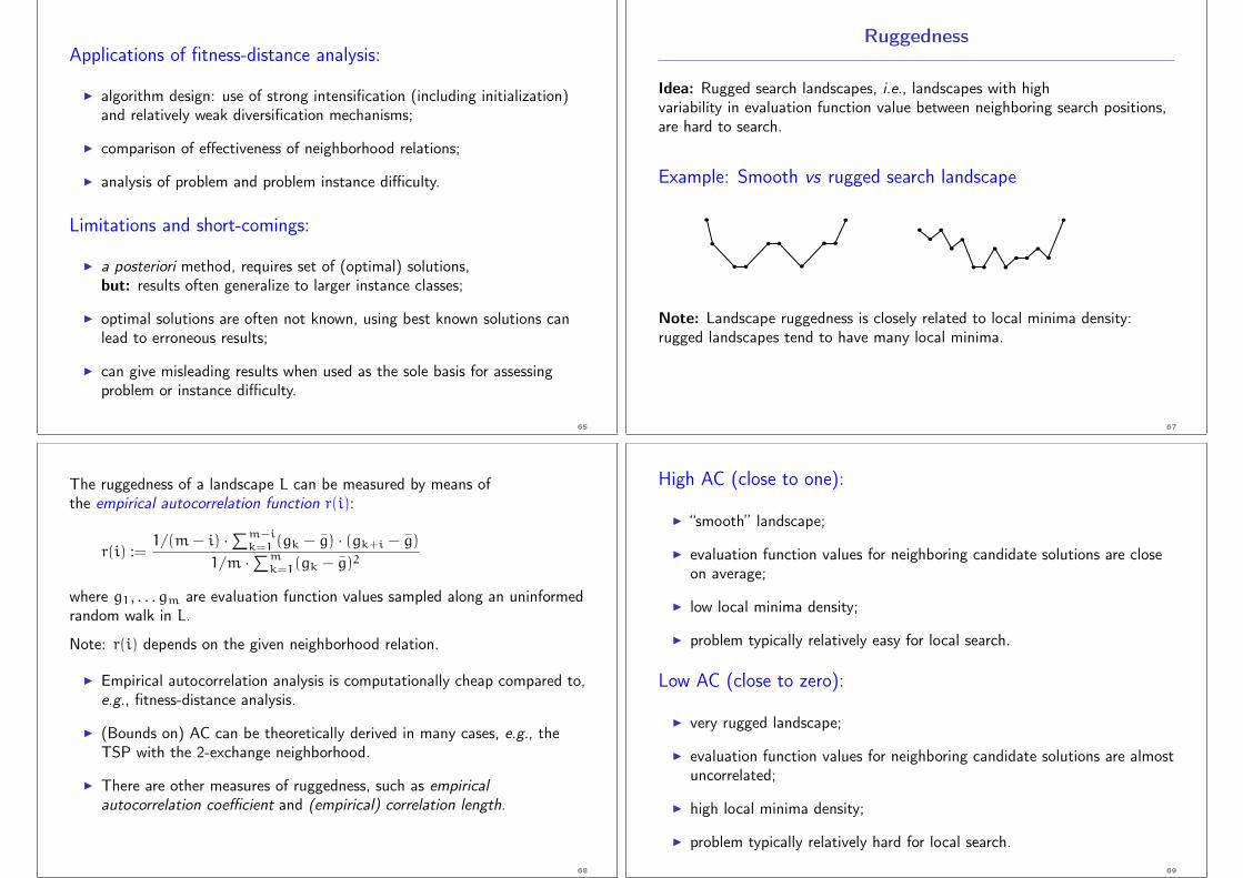
Ruggedness

Idea: Rugged search landscapes, i.e., landscapes with highvariability in evaluation function value between neighboring search positions,are hard to search.

Example: Smooth vs rugged search landscape

Note: Landscape ruggedness is closely related to local minima density:rugged landscapes tend to have many local minima.

67

The ruggedness of a landscape L can be measured by means ofthe empirical autocorrelation function r(i):

r(i) :=1/(m− i) ·∑m−i

k=1 (gk − g) · (gk+i − g)

1/m ·∑mk=1(gk − g)2

where g1, . . . gm are evaluation function values sampled along an uninformedrandom walk in L.

Note: r(i) depends on the given neighborhood relation.

I Empirical autocorrelation analysis is computationally cheap compared to,e.g., fitness-distance analysis.

I (Bounds on) AC can be theoretically derived in many cases, e.g., theTSP with the 2-exchange neighborhood.

I There are other measures of ruggedness, such as empiricalautocorrelation coefficient and (empirical) correlation length.

68

High AC (close to one):

I “smooth” landscape;

I evaluation function values for neighboring candidate solutions are closeon average;

I low local minima density;

I problem typically relatively easy for local search.

Low AC (close to zero):

I very rugged landscape;

I evaluation function values for neighboring candidate solutions are almostuncorrelated;

I high local minima density;

I problem typically relatively hard for local search.

69

Note:

I Measures of ruggedness, such as AC, are often insufficient fordistinguishing between the hardness of individualproblem instances;

I but they can be useful for

I analyzing differences between neighborhood relationsfor a given problem,

I studying the impact of parameter settings of a givenSLS algorithm on its behavior,

I classifying the difficulty of combinatorial problems.

70

Plateaux

Plateaux, i.e., ‘flat’ regions in the search landscape

Intuition: Plateaux can impede search progress due to lack of guidance bythe evaluation function.

P6.2P6.1

P5

P4.1

P4.2

P3.2

P3.1 P2

P1

P4.3

P4.4

72

Definitions

I Region: connected set of search positions.I Border of region R: set of search positions with at least one direct

neighbor outside of R (border positions).I Plateau region: region in which all positions have

the same level, i.e., evaluation function value, l.I Plateau: maximally extended plateau region,

i.e., plateau region in which no border position has anydirect neighbors at the plateau level l.

I Solution plateau: Plateau that consists entirely of solutions of thegiven problem instance.

I Exit of plateau region R: direct neighbor s of a border position of Rwith lower level than plateau level l.

I Open / closed plateau: plateau with / without exits.

73

Measures of plateau structure:I plateau diameter = diameter of corresponding subgraph of GN

I plateau width = maximal distance of any plateau position to therespective closest border position

I number of exits, exit density

I distribution of exits within a plateau, exit distance distribution(in particular: avg./max. distance to closest exit)

74

Some plateau structure results for SAT:

I Plateaux typically don’t have an interior, i.e., almost every position is onthe border.

I The diameter of plateaux, particularly at higher levels, is comparable tothe diameter of search space. (In particular: plateaux tend to span largeparts of the search space, but are quite well connected internally.)

I For open plateaux, exits tend to be clustered, but the average exitdistance is typically relatively small.

75

Barriers and Basins

Observation:

The difficulty of escaping from closed plateaux orstrict local minima is related to the height of the barrier,i.e., the difference in evaluation function, that needs to be overcome in orderto reach better search positions:

Higher barriers are typically more difficult to overcome(this holds, e.g., for Probabilistic Iterative Improvementor Simulated Annealing).

77

Definitions:

I Positions s, s ′ are mutually accessible at level liff there is a path connecting s ′ and s in the neighborhood graph thatvisits only positions t with g(t) ≤ l.

I The barrier level between positions s, s ′, bl(s, s ′)is the lowest level l at which s ′ and s ′ are mutually accessible;the difference between the level of s and bl(s, s ′) is calledthe barrier height between s and s ′.

I Basins, i.e., maximal (connected) regions of search positionsbelow a given level, form an important basis for characterizingsearch space structure.

78

Example: Basins in a simple search landscape and correspondingbasin tree

B4

B3

B1

B2

l2l1

B4

B3

B1

B2

Note: The basin tree only represents basins just below the critical levels atwhich neighboring basins are joined (by a saddle).

79

Outline





80

Efficiency vs Effectiveness

The performance of local search is determined by:

1. quality of local optima (effectiveness)

2. time to reach local optima (efficiency):

A. time to move from one solution to the next

B. number of solutions to reach local optima

82

Note:I Local minima depend on g and neighborhood function N .I Larger neighborhoods N induce

I neighborhood graphs with smaller diameter;I fewer local minima.

Ideal case: exact neighborhood, i.e., neighborhood functionfor which any local optimum is also guaranteed to bea global optimum.

I Typically, exact neighborhoods are too large to be searched effectively(exponential in size of problem instance).

I But: exceptions exist, e.g., polynomially searchable neighborhood inSimplex Algorithm for linear programming.

83

Trade-off (to be assessed experimentally):

I Using larger neighborhoodscan improve performance of II (and other LS methods).

I But: time required for determining improving search stepsincreases with neighborhood size.

Speedups Techniques for Efficient Neighborhood Search

1) Incremental updates

2) Neighborhood pruning

84

Speedups in Neighborhood Examination

1) Incremental updates (aka delta evaluations)

I Key idea: calculate effects of differences betweencurrent search position s and neighbors s ′ onevaluation function value.

I Evaluation function values often consist ofindependent contributions of solution components;hence, f(s) can be efficiently calculated from f(s ′) by differencesbetween s and s ′ in terms of solution components.

I Typically crucial for the efficient implementation ofII algorithms (and other LS techniques).

85

Example: Incremental updates for TSP

I solution components = edges of given graph GI standard 2-exchange neighborhood, i.e., neighboring

round trips p, p ′ differ in two edges

I w(p ′) := w(p) − edges in p but not in p ′

+ edges in p ′ but not in p

Note: Constant time (4 arithmetic operations), compared tolinear time (n arithmetic operations for graph with n vertices)for computing w(p ′) from scratch.

86

2) Neighborhood Pruning

I Idea: Reduce size of neighborhoods by excluding neighbors that arelikely (or guaranteed) not to yield improvements in f.

I Note: Crucial for large neighborhoods, but can be also very useful forsmall neighborhoods (e.g., linear in instance size).

Example: Heuristic candidate lists for the TSPI Intuition: High-quality solutions likely include short edges.I Candidate list of vertex v: list of v’s nearest neighbors (limited number),

sorted according to increasing edge weights.I Search steps (e.g., 2-exchange moves) always involve edges to elements

of candidate lists.I Significant impact on performance of LS algorithms

for the TSP.

87

Overview

Delta evaluations and neighborhood examinations in:

I PermutationsI TSPI SMTWTP

I AssignmentsI SAT

I SetsI Max Independent Set

89

Local Search for the Traveling Salesman Problem

I k-exchange heuristicsI 2-optI 2.5-optI Or-optI 3-opt

I complex neighborhoodsI Lin-KernighanI Helsgaun’s Lin-KernighanI DynasearchI ejection chains approach

Implementations exploit speed-up techniques1. neighborhood pruning: fixed radius nearest neighborhood search2. neighborhood lists: restrict exchanges to most interesting candidates3. don’t look bits: focus perturbative search to “interesting” part4. sophisticated data structures

90

TSP data structuresTour representation:

I determine pos of v in πI determine succ and precI check whether uk is visited between ui and ujI execute a k-exchange (reversal)

Possible choices:

I |V | < 1.000 array for π and π−1

I |V | < 1.000.000 two level treeI |V | > 1.000.000 splay tree

Moreover static data structure:I priority listsI k-d trees

91

SMTWTPI Interchange: size

(n2

)and O(|i− j|) evaluation each

I first-improvement: πj, πkpπj ≤ pπk for improvements, wjTj+wkTk must decrease because jobs

in πj, . . . , πk can only increase their tardiness.pπj ≥ pπk possible use of auxiliary data structure to speed up the com-

putationI first-improvement: πj, πk

pπj ≤ pπk for improvements, wjTj +wkTk must decrease at least asthe best interchange found so far because jobs in πj, . . . , πkcan only increase their tardiness.

pπj ≥ pπk possible use of auxiliary data structure to speed up the com-putation

I Swap: size n− 1 and O(1) evaluation eachI Insert: size (n− 1)2 and O(|i− j|) evaluation each

But possible to speed up with systematic examination by means ofswaps: an interchange is equivalent to |i− j| swaps hence overallexamination takes O(n2)

92

Example: Iterative Improvement for k-col

I search space S: set of all k-colorings of G

I solution set S ′: set of all proper k-coloring of F

I neighborhood function N : 1-exchange neighborhood(as in Uninformed Random Walk)


I initialization: uniform random choice from S, i.e., init{∅, ϕ ′} := 1/|S|

for all colorings ϕ ′

I step function:I evaluation function: g(ϕ) := number of edges in G

whose ending vertices are assigned the same color under assignment ϕ(Note: g(ϕ) = 0 iff ϕ is a proper coloring of G.)

I move mechanism: uniform random choice from improving neighbors, i.e.,step{ϕ,ϕ ′} := 1/|I(ϕ)| if s ′ ∈ I(ϕ),and 0 otherwise, where I(ϕ) := {ϕ ′ | N (ϕ,ϕ ′) ∧ g(ϕ ′) < g(ϕ)}

I termination: when no improving neighbor is availablei.e., terminate{ϕ,>} := 1 if I(ϕ) = ∅, and 0 otherwise.

93

Documents

Local Search - Politechnika Pozna„ska