IEEE Transactions on Cybernetics 1

Abstract—When solving constrained optimization problems

by evolutionary algorithms, an important issue is how to balance constraints and objective function. This paper presents a new method to address the above issue. In our method, after generating an offspring for each parent in the population by making use of differential evolution, the well-known feasibility rule is used to compare the offspring and its parent. Since the feasibility rule prefers constraints to objective function, the objective function information has been exploited as follows: if the offspring cannot survive into the next generation and if the objective function value of the offspring is better than that of the parent, then the offspring is stored into a predefined archive. Subsequently, the individuals in the archive are used to replace some individuals in the population according to a replacement mechanism. Moreover, a mutation strategy is proposed to help the population jump out of a local optimum in the infeasible region. Note that, in the replacement mechanism and the muta-tion strategy, the comparison of individuals is based on objective function. In addition, the information of objective function has also been utilized to generate offspring in differential evolution. By the above processes, this paper achieves an effective balance between constraints and objective function in constrained evolutionary optimization. The performance of our method has been tested on two sets of benchmark test functions, namely, 24 test functions at IEEE CEC2006, and 18 test functions with 10 and 30 dimensions at IEEE CEC2010. The experimental results have demonstrated that our method shows better or at least competitive performance against other state-of-the-art methods. Furthermore, the advantage of our method increases with the increase of the number of decision variables.

Manuscript received May 4, 2015; revised August 22, 2015; accepted

October 17, 2015. This work was supported in part by the National Basic Research Program 973 of China (Grant No. 2011CB013104), in part by the Innovation-driven Plan in Central South University (No. 2015CXS012 and No. 2015CX007), in part by the National Natural Science Foundation of China under Grant 61273314, Grant 51175519, and Grant 61175064, in part by RGC of Hong Kong (CityU: 11207714), in part by the Program for New Century Excellent Talents in University under Grant NCET-13-0596, and in part by State Key Laboratory of Intelligent Control and Decision of Complex Systems, Beijing Institute of Technology.

Y. Wang is with the School of Information Science and Engineering, Central South University, Changsha 410083, China, and also with the Department of Systems Engineering and Engineering Management, City University of Hong Kong, Hong Kong. (e-mail: ywang@csu.edu.cn)

B.-C. Wang is with the School of Information Science and Engineering, Central South University, Changsha 410083, China. (e-mail: bcwang@ csu.edu.cn)

H.-X. Li is with the Department of Systems Engineering and Engineering Management, City University of Hong Kong, Hong Kong, and also with the State Key Laboratory of High Performance Complex Manufacturing, Central South University, Changsha 410083, China. (e-mail: mehxli@cityu.edu.hk)

G. G. Yen is with the School of Electrical and Computer Engineering, Oklahoma State University, Stillwater, OK 74078 USA. (e-mail: gyen@ okstate.edu)

Index Terms—Constrained optimization problems, con-straints, evolutionary algorithms, objective function.

I. INTRODUCTION Without loss of generality, constrained optimization pro-

blems (COPs) can be formulated as follows: minimize ( )f xr , 1( ,..., )Dx x x S= ∈

r , i i iL x U≤ ≤ subject to: ( ) 0, 1,...,jg x j l≤ =

r ( ) 0, 1,...,jh x j l m= = +

r where xr is the decision vector, ix is the ith decision variable,

iL and iU are the lower and upper bounds of ix , respectively,

D is the number of decision variables, 1

[ , ]D

i ii

S L U=

= ∏ is the

decision space, ( )f xr is the objective function, ( )jg xr is the jth inequality constraint, ( )jh xr is the (j-l)th equality constraint, l is the number of inequality constraints, and ( )m l− is the number of equality constraints.

For COPs, the degree of constraint violation of a decision vector xr on the jth constraint is computed via the following equation:

max{0, ( )}, 1( )

max{0,| ( ) | }, 1j

jj

g x j lG x

h x l j mδ

≤ ≤⎧⎪= ⎨ − + ≤ ≤⎪⎩

rr

r (1)

where δ is a positive tolerance value to relax equality constraints to a certain extent. Then, 1( ) ( )m

jjG x G x=

= ∑r r repre-

sents the degree of constraint violation of xr on all constraints. In the context of equation (1), a decision vector xr is called a feasible solution if ( ) 0,G x =

r otherwise xr is called an infeasible solution. The decision space of a COP is composed of the feasible region and the infeasible region. The former is the set of all feasible solutions and the latter is the set of all infeasible solutions.

In the field of evolutionary computation, there has been a growing interest in applying evolutionary algorithms (EAs) to solve COPs. Due to the presence of constraints, many constrain-handling techniques have been suggested and integrated with EAs, and as a result, a variety of constrained optimization EAs (COEAs) have been proposed [1]-[3]. The current popular constraint-handling techniques can be briefly classified into three categories: methods based on penalty functions [4]-[6], methods based on the preference of feasible solutions over infeasible solutions [7]-[12], and methods based on multiobjective optimization [13]-[19]. Actually,

Yong Wang, Member, IEEE, Bing-Chuan Wang, Han-Xiong Li, Fellow, IEEE, and Gary G. Yen, Fellow, IEEE

Incorporating Objective Function Information into the Feasibility Rule for Constrained

Evolutionary Optimization

IEEE Transactions on Cybernetics 2

after producing an offspring population for the parent population by EAs, the purpose of constraint-handling techni-ques is to determine a criterion to compare the individuals in the parent and offspring populations. The methods based on penalty functions construct a fitness function by adding a penalty term proportional to the constraint violation into objective function, and then uses this fitness function to compare the individuals. In the methods based on the preference of feasible solutions over infeasible solutions, the comparison of individuals is based on either the degree of constraint violation or objective function. Moreover, feasible solutions are always considered to be better than infeasible ones to a certain degree. In addition, the methods based on multiobjective optimization transform a COP into a multi-objective optimization problem with two objectives (i.e., ( ( ), ( )))f x G xr r or a multiobjective optimization problem with (m+1) objectives (i.e., 1( ( ), ( ), , ( ))).mf x G x G xr r r

K After the above transformation, Pareto dominance is usually employed to compare the individuals.

In general, COEAs have two main tasks: 1) entering the feasible region rapidly, and 2) finding the optimal solution at the end. In order to accomplish the first task, the comparison of individuals is dependent mainly on constraints in most of constraint-handling techniques. As a result, the information of objective function has been neglected unreasonably, which has a negative effect on the achievement of the second task.

Motivated by the above consideration, this paper proposes a new COEA. We call this approach as the feasibility rule with the incorporation of objective function information (FROFI). In FROFI, differential evolution (DE) [20] serves as the search engine and the well-known feasibility rule [7] is used to compare the individuals in the population. During the evolution, if an offspring generated by DE is worse than the parent according to the feasibility rule and if the offspring has a better objective function value than its parent, the offspring will be stored into a predefined archive. Afterward, the individuals in the archive are used to replace some individuals in the population by a replacement mechanism. In addition, a mutation strategy is proposed. It is noteworthy that the comparison of individuals is based on objective function in both the replacement mechanism and the mutation strategy. Moreover, the information of objective function has also been used to guide the search in DE.

The main contributions of this paper can be summarized as: Due to the fact that the feasibility rule prefers

constraints to objective function, FROFI incorporates the objective function information into the feasibility rule by three processes, i.e., the DE operators, the replacement mechanism, and the mutation strategy. The purpose of the DE operators is to balance the exploration and exploitation abilities of FROFI. The replacement mechanism is able to diversify the population at the early stage of evolution and enhance the convergence speed at the middle and later stages of evolution. In addition, the mutation strategy aims at alleviating premature convergence in the infeasible region. By the above three processes, overall, FROFI

reaches a reasonable tradeoff between constraints and objective function.

Systematic experiments have been conducted to compare FROFI with other well-established methods on two sets of benchmark test functions, namely, 24 test functions at IEEE CEC2006 [21], and 18 test functions with 10 and 30 dimensions at IEEE CEC2010 [22]. The experimental results have indicated that FROFI is better than or at least comparable to other methods and has good scalability to the number of decision variables. Moreover, FROFI has also been applied to solve constrained mechanical design optimization problems and constrained multi-objective optimization problems.

The effectiveness of the replacement mechanism and the mutation strategy and the sensitivity of the para-meter associated with the replacement mechanism have been experimentally investigated.

The rest of this paper is organized as follows. Section II introduces DE and the feasibility rule. Section III describes the related work. The proposed method, FROFI, is elaborated in Section IV. Section V presents the performance analysis and comparison, and more experimental studies on FROFI. Finally, Section VI concludes this paper.

II. DIFFERENTIAL EVOLUTION AND THE FEASIBILITY RULE

A. Differential Evolution Differential evolution (DE) was proposed by Storn and

Price [20] in 1995. Like other EA paradigms, DE is a population-based optimization method. The population of DE can be expressed as follows:

1, ,{ ,..., }t t NP tP x x=r r (2)

where t is the generation number, NP is the population size, and , ,1, , ,( , , )i t i t i D tx x x=

rK is the ith individual. In DE, , ( {1,i tx i ∈

r , })NPK is also called a target vector. DE includes three main evolutionary operators: mutation,

crossover and selection. Mutation: The mutation operator creates a mutant vector

for each target vector through utilizing the differential information of pairwise individuals. The following two mutation operators are adopted in this paper:

DE/current-to-rand/1: , , 1, , 2, 3,( ) ( )i t i t r t i t r t r tv x F x x F x x= + ⋅ − + ⋅ −r r r r r r (3)

DE/rand-to-best/1: , 1, , 1, 2, 3,( ) ( )i t r t best t r t r t r tv x F x x F x x= + ⋅ − + ⋅ −r r r r r r (4)

where 1,..., ,i NP= 1,r 2,r and 3r are mutually different integers randomly chosen from [1, ] \ ,NP i ,best txr is the best individual in the current population, F is the scaling factor, and , ,1, , ,( , , )i t i t i D tv v v=

rK is the mutant vector.

Crossover: DE performs a crossover operator on the target vector ,i txr and its mutant vector ,i tvr to generate the trial vector , ,1, , ,( , , ).i t i t i D tu u u=

rK The binomial crossover is imple-

mented as follows:

IEEE Transactions on Cybernetics 3

, ,, ,

, ,

, if or , otherwise

i j t j randi j t

i j t

v rand CR j = ju

x≤⎧⎪= ⎨

⎪⎩ (5)

where 1,..., ,i NP= 1,..., ,j D= jrand is a uniformly distributed random number on the interval [0,1] and regenerated for each

,j randj is an integer randomly chosen from [1, ],D and CR is the crossover control parameter.

Selection: The target vector ,i txr is compared with its trial vector , ,i tur and the better one will be selected for the next generation:

, , ,, 1

,

, if ( ) ( ), otherwise

i t i t i ti t

i t

u f u f xx

x+

≤⎧⎪= ⎨⎪⎩

r r rr

r (6)

B. The Feasibility Rule The feasibility rule proposed by Deb [7] serves as the

constraint-handling technique in this paper. This rule belongs to the methods based on the preference of feasible solutions over infeasible solutions mentioned in Section I, which compares pairwise individuals as follows:

1) Between two infeasible solutions, the one with smaller degree of constraint violation is preferred;

2) If one solution is infeasible and the other one is feasible, the feasible solution is preferred;

3) Between two feasible solutions, the one with better objective function value is preferred.

III. THE RELATED WORK Recent two decades have witnessed significant progress in

the development of EAs for COPs. In 2011, Mezura-Montes and Coello Coello [3] carried out a comprehensive survey on constraint-handling in nature-inspired numerical optimization. Recent developments during the last four years are briefly outlined below.

1) Methods based on penalty functions: Kusakci and Can [23] integrated a modified covariance matrix adaptation evolution strategy (CMA-ES) [24] with a penalty approach introduced in [4]. de Melo and Iacca [25] modified the stopping criteria and the sampling mechanism of CMA-ES [24], and introduced an adaptive penalty function into the modified CMA-ES. Ali and Zhu [26] proposed a constrained DE equipped with penalty function. Moreover, they provided theoretical results about the setting of the penalty coefficient. Hernández et al. [27] proposed a hybridization of DE and hill climbing, which employs static penalty to deal with constraints. In [28], a rough penalty method inspired by Pawlak’s rough set theory [29] is proposed and coupled with an improved genetic algorithm. Li and Zhang [30] proposed an interesting piece of work, in which the minimum penalty coefficient is estimated at each generation. Wang and Cai [31] proposed (μ+λ)-CDE, which divides the evolutionary process into three situations: infeasible situation, semi-feasible situation, and feasible situation. In the semi-feasible situation, an adaptive penalty function is devised. Based on the constraint-handling framework in [31], Gong et al. [32] proposed two improvements: a ranking-based mutation operator of DE and a dynamic diversity mechanism.

2) Methods based on the preference of feasible solutions over infeasible solutions: At present, some researchers focus mainly on how to design the search algorithms and the feasibility rule is directly employed or slightly revised to handle constraints. For example, Gordián-Rivera and Mezura-Montes [33] proposed an approach to combine three DE variants, in which the three DE variants compete to generate offspring based on two performance measures. Mezura-Montes and Lopez-Davila [34] designed an adaptive stepsize control and a local search operator, and put them into the modified bacterial foraging algorithm (BFOA) [35]. Hernández-Ocaña et al. [36] added four stepsize control mechanisms into the modified BFOA [35]. Elsayed et al. carried out a series of work on combining multiple algorithms and/or multiple operators to tackle constrained search space, such as a self-adaptive multi-strategy DE [37] and an ada-ptive configuration of EAs [38]. Sarker et al. [39] developed a DE with dynamic parameter selection. In this method, three sets of parameters are considered: the first set is for the scaling factor F, the second is for the crossover control parameter CR, and the third is for the population size NP. Zhang et al. [40] developed a constrained artificial immune system based on immune response principle, in which the population is classified into the feasible and infeasible groups. Tuba and Bacanin [41] hybridized improved seeker optimi-zation algorithm [42] with firefly algorithm [43]. Sadollah et al. [44] introduced a new metaheuristic algorithm, called the mine blast algorithm. Mohamed and Sabry [45] implemented several modifications on DE, including the mutation operator, F, and CR. Recently, Dhadwal et al. [46] proposed an advanced particle swarm assisted genetic algorithm.

The ε constrained method proposed by Takahama and Sakai [47] is another representative constraint-handling technique belonging to the methods based on the preference of feasible solutions over infeasible solutions. In 2012, Takahama and Sakai [48] selected different values of F and CR for each individual in DE according to the rank of the base vector, and proposed a rank-based εDE. In 2013, Takahama and Sakai [49] combined the ε constrained method with the estimated comparison using kernel regression. Recently, Bu et al. [50] implemented an improved version of εDEag [51] by utilizing the species based repair strategy. Dominguez-Isidro et al. [52] proposed a memetic algorithm, in which DE is used as the global search algorithm and the local search is implemented by a mathematical programming method. In addition, the ε constrained method is applied to compare the individuals.

3) Methods based on multiobjective optimization: Currently, this kind of methods usually converts a COP into a biobjective optimization problem like ( ( ), ( )).f x G xr r After the above transformation, Dong and Wang [53] constructed the achievement scalarizing function [54]:

1 1 2 2( ) max{ ( ( ) ), ( ( ) )}F x f x z G x zω ω= − −r r r (7)

where 1 2( , )ω ω ω=r is a weighting vector and 1 2( , )z z z=r is a

reference point. They imposed preference to ( )f xr and ( )G xr via different weighting vectors and reference points (i.e., a

IEEE Transactions on Cybernetics 4

preference based biobjective optimization). Jiao et al. [55] proposed a novel selection strategy. After combining the offspring population with the parent population, this selection strategy firstly eliminates the individuals with higher con-straint violations than the maximum constraint violation of the last generation, and subsequently the nondominated indi-viduals are chosen. Wang and Cai [56] presented a dynamic hybrid framework referred as DyHF, in which the global and local search models are dynamically implemented according to the feasibility proportion of the population. In the same year, Wang and Cai [57] proposed CMODE, which combines multiobjective optimization with DE. The above two methods adopts Pareto dominance to compare the individuals.

4) Methods based on hybrid constraint-handling tech-niques: Deb and Datta [58] proposed a hybrid evolutionary and penalty function method. This method firstly converts a COP into a biobjective optimization problem. Afterward, NSGA-II [59] is used to solve the converted problem and the nondominated front is applied to estimate the penalty coeffi-cient. In [60], the main framework is inherited from [58], but the previous gradient-based approach is replaced with a gradient-free pattern search approach. Datta and Deb [61] studied on the scaling issue in constrained optimization and proposed an adaptive normalization technique for constraints. Subsequently, this technique is integrated with a hybrid method similar to [58]. Cai et al. [62] introduced a novel memetic algorithm called IWO-DE. In IWO-DE, an adaptive fitness function is designed to determine the reproduction ability of each weed in IWO [63]. If the population size of IWO reaches the permissible maximum, some worst indivi-duals are removed by the nondominated sorting [59]. Later, Hu et al. [64] extended the above work by making use of a ring neighborhood topology as the population structure. Li and Yin [65] proposed a self-adaptive constrained artificial bee colony algorithm, in which the employed bee colony based on the feasibility rule is responsible for global search and the onlooker bee colony based on multiobjective optimi-zation is treated as the local search model.

IV. PROPOSED APPROACH

A. Motivation Balancing constraints and objective function is a

fundamental issue in constrained evolutionary optimization. The methods based on penalty functions attempt to address this issue by introducing appropriate penalty coefficients into the penalty term. In addition, the methods based on multiobjective optimization tend to strike a balance by converting a COP into a multiobjective optimization problem. However, in the methods based on the preference of feasible solutions over infeasible solutions, this issue has not been well studied. For example, despite the feasibility rule being the most popular constraint-handling technique during the last four years, more focus has been put on the search algorithms when using it to solve COPs as pointed out previously. The reason seems straightforward: the feasibility rule prefers constraints to objective function and may cause

problems such as premature convergence, especially when solving complex COPs, and as a result, it is expected to design more powerful search algorithms to overcome its limitation to a certain degree. In principle, the feasibility rule is a relatively greedy constrain-handling technique. Note, however, that its greedy property also leads to some attracted advantages over other kinds of constraint-handling techniques, such as the capabilities to rapidly motivate the population toward the feasible region and to speed up the optimization in the promising directions.

In view of the fast but less reliable constraint-handling performance of the feasibility rule, a new method named FROFI is proposed which utilizes the information provided by objective function to alleviate the greediness and improve the robustness. Moreover, by incorporating the objective function information into the feasibility rule, FROFI can reach an effective balance between constraints and objective function.

B. FROFI At each generation ,t FROFI maintains:

Input: :NP the population size :poolF the pool of the scaling factor F

:poolCR the pool of the crossover control parameter CR

:MaxFEs maximum number of fitness evaluations 1: 1t = ; /* t denotes the generation number */ 2: Randomly generate an initial population 1, ,{ , , }t t NP tP x x=

r rK from the

decision space ;S 3: Evaluate the f value and the G value for each individual in ;tP

/* f and G denote the objective function and the degree of constraint violation, respectively */

4: ;FEs NP= /* FEs denotes the number of fitness evaluations */ 5: 1tP+ = Ø and A = Ø;

6: For each individual ,i txr (also called a target vector) in tP /* {1, 2,..., }i NP= */

7: Randomly select a value from poolF for the scaling factor ,F

randomly select a value from poolCR for the crossover control

parameter ,CR and implement the mutation and crossover operators of DE introduced in Fig. 2 to generate the trial vector , ;i tur

8: Evaluate the f value and the G value for ,i tur and set

1;FEs FEs= +

9: Compare ,i txr with ,i tur according to the feasibility rule and store the

better one into 1;tP+

10: If ,i tur cannot survive into 1tP+ and if , ,( ) ( ),i t i tf u f x<r r then

, ;i tA A u=r

U 11: End For 12: Replace some individuals in 1tP+ with the individuals in A according

to the replacement mechanism introduced in Fig. 4; 13: Implement the mutation strategy introduced in Fig. 5 and set

1;FEs FEs= + 14: 1;t t= + 15: Stopping Criterion: If ,FEs MaxFEs≥ then stop and output the best

individual in ,tP otherwise go to step 5.

Fig. 1. The framework of FROFI

IEEE Transactions on Cybernetics 5

a population of NP individuals: 1, ,{ , , };t t NP tP x x=r r

K the objective function values of :tP 1, ,( ), , ( );t NP tf x f xr r

K the degree of constraint violation of :tP 1,( ), ,tG xr K

,( ).NP tG xr COEAs include two main components, i.e., the constraint-

handling technique and the search algorithm. Due to its numerous advantages, including simplicity, efficiency, and ease of implementation, DE has been utilized as the search algorithm in FROFI. The framework of FROFI has been given in Fig. 1. During the evolution, for each individual ,i txr (also called a target vector) in ,tP a trial vector ,i tur is gene-rated by making use of the mutation and crossover operators of DE. Afterward, ,i txr is compared with ,i tur based on the feasibility rule, and the better one is selected and put into the next population 1.tP+ If ,i tur cannot survive into 1tP+ and if

, ,( ) ( ),i t i tf u f x<r r then ,i tur will be stored into a predefined

archive .A Under this condition, the properties of ,i tur can be summarized as follows.

Theorem 1: ,i tur is an infeasible individual. Proof: Assume that ,i tur is a feasible individual. Since

,i tur is worse than ,i txr based on the feasibility rule, the following condition holds: ,i txr is also a feasible individual and , ,( ) ( ).i t i tf x f u<

r r This is in contradiction to the fact that

, ,( ) ( ).i t i tf u f x<r r After the update of 1tP+ has been completed, the indivi-

duals in A are used to replace some individuals in 1tP+ by a replacement mechanism. Subsequently, a mutation strategy is implemented. The above procedure is repeated until the maximum number of fitness evaluations (FEs) is reached.

Next, we will explain the DE operators, the replacement mechanism, and the mutation strategy in detail.

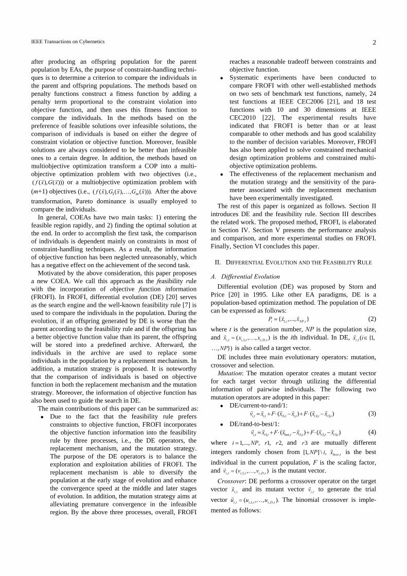
C. DE operators In FROFI, two DE mutation operators introduced in

Section II-A (i.e., DE/current-to-rand/1 and DE/rand-to-best/1) are adopted, each of which is applied with the same probability (i.e., 0.5) when producing the mutant vector ,i tvr for a target vector , .i txr In DE/current-to-rand/1, the current

individual learns the information from other randomly chosen individuals. However, in DE/rand-to-best/1 the information of the best individual in the population is also utilized. In order to further improve the search performance, the first scaling factor in both of them is set to a uniformly distributed random number between 0 and 1. Note that after mutation, the binomial crossover of DE is only applied to DE/rand-to-best/1. DE/current-to-rand/1 without the binomial crossover is a rotation-invariant process and very effective for solving the rotated problems [66]. The details of the DE mutation and crossover operators have been given in Fig. 2.

As shown in Fig. 2, the best individual (i.e., , )best txr in DE/rand-to-best/1 is determined according to objective func-tion. The reasons are listed as follows:

At the early stage of evolution, the population may contain only infeasible solutions. Due to that fact that in this scenario the population should continuously approach the feasible region to find a feasible solution, the infeasible individual with the best objective function value may change from generation to generation in the evolutionary process. As a result,

,best txr somehow likes a randomly selected individual. Under this condition, both DE/rand-to-best/1 and DE/ current-to-rand/1 play a similar role, i.e., promoting the global exploration ability of the population.

At the middle and later stages of evolution, more and more individuals in the population become feasible. If a feasible individual has the best objective function value, then the population will be promptly guided toward this promising solution. On the other hand, if an infeasible individual near the feasible region has the best objective function value, it is very likely that the optimal solution is located on the boundary of the feasible region. In this case, by utilizing such infeasible individual, a lot of potential infeasible individuals may be generated near the feasible region, which provides an advantage to search for the optimal solution by surrounding the boundary of the feasible region from both the feasible and infeasible sides. A COP has been taken as an example in Fig. 3, where *xr denotes the optimal solution located on the boundary

The feasible region

*xr

**xr

^xr  

Fig. 3. Schematic diagram of a COP. The dashed ellipses display the contours of objective function, *xr denotes the optimal solution of this COP which is located on the boundary of the feasible region, **xr denotes the unconstrained optimal solution, circles denote the feasible individuals, ^xr

denotes the infeasible individual with the best objective function value, and triangles denote some potential infeasible individuals near the feasible region which are generated through exploiting ^.xr

1: If 0.5rand < /* rand is a uniformly distributed random number between 0 and 1 */

2: , , 1, , 2, 3,( ) ( );i t i t r t i t r t r tv x rand x x F x x= + ⋅ − + ⋅ −r r r r r r /* DE/current-to-rand/1 */

3: , , ;i t i tu v=r r

4: Else 5: , 1, , 1, 2, 3,( ) ( ),i t r t best t r t r t r tv x rand x x F x x= + ⋅ − + ⋅ −

r r r r r r where ,best txr is the best individual of the population in terms of objective function; /* DE/rand-to-best/1 */

6: Execute the binomial crossover of DE on ,i txr and ,i tvr to

generate the trial vector , ;i tur 7: End If

Fig. 2. The mutation and crossover operators of DE in FROFI

IEEE Transactions on Cybernetics 6

of the feasible region and ^xr denotes the infeasible individual with the best objective function value. As shown in Fig. 3, some potential infeasible individuals near the feasible region (denoted as triangles) may be generated via making use of ^.xr

Based on the above discussion, it is beneficial to use the information provided by objective function to guide the search in DE. By doing this, the global search ability can be strengthened at the early stage and the local exploitation can be encouraged at the middle and later stages.

D. Replacement Mechanism The replacement mechanism aims at alleviating the

greediness of the feasibility rule by replacing some indivi-duals in the population with the individuals in the archive .A

In order to avoid the replacement occurrence only in a small area of the decision space, a simple way is proposed in which we divide the population into MRN parts with the same size, after sorting it based on the objective function values in descending order. This way can be regarded as a very simple and cheap niching technique [67] because the objective function values of the neighboring individuals may be very similar. Subsequently, we choose the individual with the maximum degree of constraint violation from the first part (denoted as )axr and the individual with the minimum degree of constraint violation from A (denoted as ),bxr respectively. If ( ) ( ),b af x f x<

r r bxr is stored into the population by replacing

axr and then deleted from .A Next, the individual with the maximum constraint violation

value in the second part (also denoted as )axr and the individual with the minimum constraint violation value in A (also denoted as bxr ) are selected. Similarly, if ( ) ( ),b af x f x<

r r

axr is replaced with bxr and bxr is subsequently removed from .A The above process continues until all the MRN parts are

updated or A becomes an empty set. Therefore, MRN determines the maximum replacement number. Fig. 4 shows the implementation of the replacement mechanism.

The advantages of the replacement mechanism are twofold:

If the population contains only infeasible individuals, it is helpful to maintain the diversity of the population and guide the population toward the feasible region from diverse directions, by making use of the individuals in A to replace some individuals of the population located in different areas based on objective function.

For a kind of COPs in which one or several constraints are active at the optimal solution, the optimal solution is located precisely on the boundary of the feasible region. Under this condition, by comparing the individuals based on objective function in the replacement mechanism, the infeasible individuals in the vicinity of the optimal solution are very likely to enter the next population, provided that the objective function values of such infeasible individuals are less than those of the feasible individuals. As pointed out by Mezura-Montes and Coello Coello [8], it is very promising to quickly find the optimal solution located on the boundary of the feasible region by combining the infeasible individuals with the feasible individuals close to the optimal solution.

E. Mutation Strategy The constraints of some COPs exhibit nonlinear and

multimodal properties. As a result, if only the information of constraints is considered, the population will be easily trapped into a local optimum in the infeasible region and fea-sible solutions cannot be found when the iteration terminates. In this case, the objective function information may be useful for the population to jump out of a local optimal basin in the infeasible region.

Based on the above consideration, a simple mutation strategy is proposed. It is necessary to emphasize that this mutation strategy is only applied to the situation that all the individuals in the population are infeasible. Firstly, let cxr be an individual chosen from the population at random, exr the individual with the maximum degree of constraint violation in the population, and k an integer number randomly selected from [1, ].D Then, a random number between kL and

kU is assigned to the kth dimension of cxr and thus a mutated

1: Sort 1tP+ in descending order according to the objective function values and divide it into MRN parts with the same size;

2: 1;i = 3: While 0A > and i MRN≤

/* A denotes the cardinality of A */ 4: Select the individual with the maximum degree of constraint

violation (denoted as axr ) from the ith part of 1;tP+ 5: Select the individual with the minimum degree of constraint

violation (denoted as bxr ) from ;A

6: If ( ) ( )b af x f x<r r

7: 1 1 \t t aP P x+ +=r and 1 1 ;t t bP P x+ +=

rU

8: \ ;bA A x=r

9: End If 10: 1;i i= + 11: End While

Fig. 4. The replacement mechanism in FROFI

1: If all the individuals in the population are infeasible 2: Randomly select an individual (denoted as cxr ) from 1;tP+ 3: Generate a random integer number (denoted as )k between 1

and ,D and let the kth dimension of cxr be equal to a value

randomly chosen from [ , ].k kL U Thus, a mutated individual dxr is obtained;

4: Evaluate the f value and the G value for ;dxr 5: Choose the individual with the maximum degree of constraint

violation (denoted as exr ) in 1;tP+

6: If ( ) ( )d ef x f x<r r

7: 1 1 \t t eP P x+ +=r and 1 1 ;t t dP P x+ +=

rU

8: End If 9: End If

Fig. 5. The mutation strategy in FROFI

IEEE Transactions on Cybernetics 7

individual is generated (denoted as dxr ). Afterward, if ( )df x <r

( ),ef xr dxr will enter the population by replacing .exr Fig. 5 presents the detailed explanations of the mutation strategy.

Remark: From the above introduction, the implementation of FROFI is simple and it does not impose any com-putationally expensive operations. The computational time complexity of FROFI is ( log( )),O NP NP which is governed by the sorting in the replacement mechanism.

F. Analysis of the Principle As introduced previously, the feasibility rule and multi-

objective optimization are two kinds of popular constraint-handling techniques, and the aim of FROFI is to incorporate the objective function information into the feasibility rule. Indeed, the above three methods have a similarity, i.e., they treat the constraints and objective function separately. Table I discusses the principles of the feasibility rule, multiobjective optimization, and FROFI when comparing a parent ixr with an offspring .iur Note that Pareto dominance is used to compare ixr and iur when a COP is transformed into a multiobjective optimization problem.

As shown in Table I, if both ixr and iur are feasible solutions, then all the above three methods put the importance of 100% on the objective function and the constraint violation can be ignored. However, if one of ixr and iur is infeasible or both of them are infeasible, the feasibility rule lies on one extreme, i.e., minimizing the constraint violation is consi-dered more important than minimizing the objective function. Meanwhile, multiobjective optimization lies on the other extreme, i.e., the constraint violation and objective function are of equal importance. Under this condition, FROFI first compares iur with ixr based on the feasibility rule. Afterward, if iur is worse than ixr in terms of the constraint violation and better than ixr in terms of the objective function, iur will be stored into the archive and utilized in the subsequent evolution, which means that the constraint violation plays a primary role and the objective function plays an auxiliary role. Therefore, FROFI lies between the above two extremes, which is an advantage of FROFI in principle as compared to the feasibility rule and mutiobjective optimization.

V. EXPERIMENTAL STUDY

A. Proof-of-Principle Results Firstly, three artificial test functions are constructed to

capture some important characteristics of introducing the objective function information into the feasibility rule in FROFI. These test functions contain two decision variables, and consequently, are easy to visualize. In order to further compare FROFI with the feasibility rule and multiobjective optimization, two FROFI variants referred as FROFI_FR and FROFI_MO are designed. In FROFI_FR and FROFI_MO, the comparison of individuals is based on the feasibility rule and Pareto dominance, respectively. For both of them, the following two steps ae implemented: 1) the archiving and replacement are removed from FROFI, and 2) the mutation strategy is removed from FROFI. In addition, ,best txr of DE/ rand-to-best/1 in Fig. 2 represents the best individual in the population based on the feasibility rule for FROFI_FR, and one of the nondominated individuals in the population for FROFI_MO. Moreover, DE/current-to-rand/1 in Fig. 2 is kept unchanged for FROFI_FR and FROFI_MO.

The three artificial test functions have the following formulations:

2 21 21

1

1

1 2

ATF1: minimize ( ) 10cos(2 ) 10, 5 , 5

subject to: +2 0 3 0 2 7 0

i iif x x x x x

xxx x

π=

= − + − ≤ ≤

≤− − ≤

+ + =

∑r

2 21

1 22 2

1 22 2

1 2

ATF2: minimize ( ) 10cos(2 ) 10,

10 5, 5 5

subject to: 3( 7) 0.3 or

( 8) ( 3) 2

i iif x x x

x x

x x

x x

π=

= − +

− ≤ ≤ − ≤ ≤

+ + ≤

+ + − ≤

∑r

x1

x 2

-5 0 5-5

0

5

The feasible region

x1

x 2

-10 -5 0 5-5

0

5The feasible region

The optimal solution

(a) ATF1 (b) ATF2

x1x 2

-10 -5 0 5-5

0

5

The feasible region

The optimal solution

(c) ATF3

Fig. 6. The search space, the contours of objective function, the feasible region, and the optimal solution of the three artificial test functions

TABLE I THE PRINCIPLES OF THE FEASIBILITY RULE, MULTIOBJECTIVE OPTIMIZATION, AND FROFI WHEN COMPARING A PARENT ixr WITH AN OFFSPRING iur

Comparison of ixr and iur The feasibility rule Multiobjective optimization FROFI

ixr & iur are infeasible One is feasible and the other

one is infeasible

The importance of the constraint violation is 100% and the importance

of the objective function is 0%

The importance of both the constraint violation and objective

function is 50%

The constraint violation plays a primary role and the objective function plays an auxiliary role

ixr & iur are feasible The importance of the objective

function is 100% and the importance of the constraint violation is 0%

The importance of the objective function is 100% and the importance

of the constraint violation is 0%

The importance of the objective function is 100% and the importance

of the constraint violation is 0%

IEEE Transactions on Cybernetics 8

2 21

1 22 2

1 2

ATF3: minimize ( ) 10cos(2 ) 10,

10 5, 5 5

subject to: 3( 9) 2

i iif x x x

x x

x x

π=

= − +

− ≤ ≤ − ≤ ≤

+ + ≤

∑r

It is evident that these three test functions have the same objective function, which is the Rastrigin function with 2D [68]. The search space, the contours of objective function, the feasible region, and the optimal solution of them have been presented in Fig. 6.

When solving these three test functions, the population size NP was set to 40 and other parameter settings were kept unchanged which will be specified in Section V-B. Moreover, FROFI, FROFI_FR, and FROFI_MO used the same initial population to ensure the comparison fair. Figs. 7-15 provide a typical run derived from them on ATF1, ATF2, and ATF3. From Figs. 7-15, we can observe:

As depicted in Fig. 7, FROFI_FR approaches the feasible region of ATF1 from only one side along with the evolution. In contrast, FROFI is able to approach the feasible region of ATF1 from both sides as shown in Fig. 9.

From Fig. 10, FROFI_FR concentrates its search around the feasible area with a relatively larger size of ATF2 and runs the risk of getting stuck at a local feasible optimal solution. On the contrary, the search of FROFI is carried out around the two parts of the feasible region of ATF2 and finally the global optimal solution can be found as shown in Fig. 12.

It is clear from Fig. 13 that FROFI_FR enters the feasible region of ATF3 with a very fast speed and all the individuals in the population promptly become feasible. Due to the lack of sufficient sampling in the area including the optimal solution, FROFI_FR is prone to converge to a local attraction basin of the feasible region. As shown in Fig. 15, a lot of effort has been made by FROFI on both the feasible and infea-sible areas around the optimal solution, and as a result, FROFI succeeds in locating the optimal solution.

When comparing two infeasible individuals based on Pareto dominance, they may be frequently nondo-minated with each other. Due to such low selection pressure, it is a very challenging task for FROFI_MO to find feasible solutions, see, for example, Fig. 8, Fig. 11, and Fig. 14. Specifically, for ATF1, FROFI_MO cannot find a feasible solution even the generation number is equal to 500. For ATF2, FROFI_MO fails to find a feasible solution in the small part of the feasible region. In addition, FROFI_MO is unable to provide a feasible solution for ATF3. As pointed out in [12], a search bias toward the feasible region should be introduced into multiobjective optimization for locating feasible solutions of COPs.

Overall, by incorporating the objective function infor-mation into the feasibility rule, FROFI is capable of enhancing the diversity of the population and steering the population toward the feasible region from diverse directions (for instance ATF1 and ATF2). Moreover,

t=1

x1

x 2

-5 0 5-5

0

5 t=8

x1

x 2

-5 0 5-5

0

5 t=10

x1

x 2

-5 0 5-5

0

5

Fig. 7. The evolution of FROFI_FR over a typical run on ATF1. Hereinafter, t denotes the generation number.

t=1

x1

x 2

-5 0 5-5

0

5 t=100

x1

x 2

-5 0 5-5

0

5 t=500

x1

x 2-5 0 5

-5

0

5

Fig. 8. The evolution of FROFI_MO over a typical run on ATF1 t=1

x1

x 2

-5 0 5-5

0

5 t=8

x1

x 2

-5 0 5-5

0

5 t=10

x1

x 2

-5 0 5-5

0

5

Fig. 9. The evolution of FROFI over a typical run on ATF1

x1

x 2

t=1

-10 -5 0 5-5

0

5

x1

x 2

t=30

-10 -5 0 5-5

0

5

x1

x 2

t=50

-10 -5 0 5-5

0

5

Fig. 10. The evolution of FROFI_FR over a typical run on ATF2

x1

x 2

t=1

-10 -5 0 5-5

0

5

x1

x 2

t=30

-10 -5 0 5-5

0

5

x1

x 2

t=50

-10 -5 0 5-5

0

5

Fig. 11. The evolution of FROFI_MO over a typical run on ATF2

x1

x 2

t=1

-10 -5 0 5-5

0

5

x1

x 2

t=30

-10 -5 0 5-5

0

5

x1

x 2

t=50

-10 -5 0 5-5

0

5

Fig. 12. The evolution of FROFI over a typical run on ATF2

x1

x 2

t=1

-10 -5 0 5-5

0

5

x1

x 2

t=30

-10 -5 0 5-5

0

5

x1

x 2

t=50

-10 -5 0 5-5

0

5

Fig. 13. The evolution of FROFI_FR over a typical run on ATF3

x1

x 2

t=1

-10 -5 0 5-5

0

5

x1

x 2

t=30

-10 -5 0 5-5

0

5

x1

x 2

t=50

-10 -5 0 5-5

0

5

Fig. 14. The evolution of FROFI_MO over a typical run on ATF3

x1

x 2

t=1

-10 -5 0 5-5

0

5

x1

x 2

t=30

-10 -5 0 5-5

0

5

x1

x 2

t=50

-10 -5 0 5-5

0

5

Fig. 15. The evolution of FROFI over a typical run on ATF3

IEEE Transactions on Cybernetics 9

it is an effective method to find the optimal solution located on the boundary of the feasible region from both feasible and infeasible parts (for instance ATF3).

To summarize, the above experiments present detailed insights into why FROFI is able to overcome the weaknesses of the two extremes in the feasibility rule and multiobjective optimization. The experiment comparisons among FROFI, FROFI_FR, and FROFI_MO on the benchmark test functions introduced in Section V-B have been summarized in the supplemental file (Tables S1-S3).

B. Benchmark Test Functions and Parameter Settings Next, we employed two sets of benchmark test functions to

thoroughly evaluate the performance of FROFI and to compare FROFI with other state-of-the-art COEAs. The first set is the 24 benchmark test functions collected in IEEE CEC2006 [21], and the second set is the 18 benchmark test functions with 10 dimensions (10D) and 30 dimensions (30D) developed in IEEE CEC2010 [22]. Note that the objective function of all the test functions should be minimized. The details of these test functions can be found in [21] and [22].

In the experimental study of FROFI, the maximum number of FEs MaxFEs and the population size NP were given in Table II. Note that a proper setting of the population size is related to the dimension of an optimization problem. As

shown in Table II, for the 10D test functions, a slightly smaller population size was adopted to make FROFI more efficient. In addition, 25 independent runs were performed for each test function and the tolerance value δ for equality constraints was set to 0.0001. It is necessary to point out that the settings of ,MaxFEs the number of runs, and the tolerance value δ are based on the suggestions in [21] and [22], and kept the same in all the compared methods. Inspired by [66], we established a scaling factor pool (i.e., poolF = [0.6,0.8,1.0]) and a crossover control parameter pool (i.e., [0.1,0.2,poolCR = 1.0]) in DE. At each generation, we randomly chose a value from poolF for F and a value from poolCR for CR. Then, the mutation and crossover operators of DE were implemented based on the chosen F and CR values. FROFI introduces a maximum replacement number MRN in the replacement mechanism. In all simulations, MRN=max(5,D/2) which implies that when D>10, MRN=D/2, otherwise MRN=5.

C. Experiments on the 24 Benchmark Test Functions Collected in IEEE CEC2006

For the 24 benchmark test functions (denoted as g01-g24) collected in IEEE CEC2006, the performance of FROFI was compared with that of five state-of-the-art methods: εDE [47], APF-GA [69], (μ+λ)-CDE [31], DyHF [56], and CMODE [57]. The experimental results of these five methods were directly taken from the original papers for fair comparison.

For each test function, a run is successful if the following success condition is satisfied: *( ) ( ) 0.0001bestf x f x− ≤

r r and

bestxr is feasible, where *xr is the best known solution and bestxr is the best solution provided by an algorithm. Similar to [31], [56], and [57], FROFI finds an improved best known solution for g17, the objective function value of which is 8853.53387481. Therefore, this improved best known solution is used to compute the success condition for g17. Regarding g20, no feasible solution has been reported by the existing algorithms. Moreover, the decrease of constraint violation of an individual in the vicinity of the optimal solution will result in the increase of its objective function value. Thus, for g20 the success condition is revised to

*| ( ) ( ) | 0.0001.bestf x f x− ≤r r

According to the suggestion in [21], we used the success rate and the success performance as the performance indicators to compare εDE, APF-GA, (μ+λ)-CDE, DyHF, CMODE, and FROFI. The success rate is the percentage of successful runs, and the success performance is the mean number of FEs for successful runs divided by the success rate. The success rates resulting from the six compared methods are summarized in the supplemental file (Table S4). As shown in the supplemental file, εDE, APF-GA, (μ+λ)-CDE, DyHF, CMODE, and FROFI achieve 100% success rate on 22, 12, 21, 22, 22, and 23 test functions, respectively. In this regard, FROFI shows the most stable performance. Moreover, FROFI provides the highest mean success rate (i.e., 95.83%).

The success performance of the six compared methods is also summarized in the supplemental file (Table S5), in

TABLE II THE MAXIMUM NUMBER OF FES MaxFEs AND THE POPULATION SIZE NP

Test Function MaxFEs NP

24 test functions from IEEE CEC2006 5.0E+05 80

18 test functions with 10D from IEEE CEC2010 2.0E+05 60

18 test functions with 30D from IEEE CEC2010 6.0E+05 80

TABLE III

RESULTS OF THE MULTIPLE-PROBLEM WILCOXON’S TEST BASED ON THE SUCCESS PERFORMANCE FOR εDE [47], APF-GA [69], (μ+λ)-CDE [31], DYHF [56], CMODE [57], AND FROFI ON 24 TEST FUNCTIONS FROM

IEEE CEC2006

Algorithm R+ R- p-value α=0.05 α=0.1 FROFI vs εDE 203.0 73.0 4.84E-02 Yes Yes

FROFI vs AGF-GA 269.0 7.0 4.53E-06 Yes Yes FROFI vs (μ+λ)-CDE 245.0 31.0 5.52E-04 Yes Yes

FROFI vs DyHF 208.5 67.5 3.14E-02 Yes Yes FROFI vs CMODE 245.5 30.5 5.14E-04 Yes Yes

TABLE IV

RANKING OF εDE [47], APF-GA [69], (μ+λ)-CDE [31], DYHF [56], CMODE [57], AND FROFI BY THE FRIEDMAN’S TEST IN TERMS OF THE SUCCESS PERFORMANCE ON 24 TEST FUNCTIONS FROM IEEE CEC2006

Algorithm Ranking

FROFI 2.2708 εDE 2.75

DyHF 2.8542 CMODE 3.6458

(μ+λ)-CDE 4.0833 AGF-GA 5.3958

IEEE Transactions on Cybernetics 10

which “NA” denotes the success performance of the corresponding method cannot be available since the success rate is equal to zero. To detect the statistical differences systematically, the multiple-problem Wilcoxon’s test and the Friedman’s test [70] were carried out by making use of keel software [71]. In the Friedman’s test, the Bonferroni-Dunn method was chosen for the post-hoc test. Tables III and IV summarize the statistical test results based on the success performance. From Table III, we can observe that FROFI provides higher R+ values than R- values in all the cases. Moreover, the p values of all the cases are less than 0.05, which indicates that FROFI exhibits statistically superior convergence performance against the five competitors. In addition, it can be seen from Table IV that FROFI works best, followed by εDE.

The above comparison verifies that FROFI is better than the five competitors on the 24 benchmark test functions from IEEE CEC2006, in terms of the success rate and the success performance.

D. Experiments on the 18 Benchmark Test Functions with 10D and 30D Designed in IEEE CEC2010

In this subsection, we compared FROFI against six competitive methods on the 18 test functions (denoted as C01-C18) with 10D and 30D from IEEE CEC2010 to validate its performance: εDEag [51], SRS-εDEag [50], ECHT-DE [72], AIS-IRP [40], DyHF [56], and CMODE [57].

Unlike the test functions in Section V-C, the optimal solutions of these 18 test functions cannot be known a priori. Consequently, the average and standard deviation of the objective function values obtained in 25 runs were considered as the performance indicator. The supplemental file (Tables S6-S9) summarizes the experimental results provided by the

six compared methods. Herein, “*” denotes that feasible solutions cannot be consistently found by the corresponding method in all runs, and (#) denotes the feasible rate which is the percentage of runs where at least one feasible solution is found when the evolution halts. The experimental results of εDEag, SRS-εDEag, ECHT-DE, and AIS-IRP were directly taken from the original papers. For DyHF and CMODE, we run the source codes provided by the authors in [56] and [57] to produce the experimental results due to the fact that the experimental results cannot be obtained from [56] and [57].

To test the statistical significance, t-test at a 0.05 significance level was conducted between FROFI and each of εDEag, SRS-εDEag, ECHT-DE, and AIS-IRP. In addition, Wilcoxon’s rank sum test at a 0.05 significance level is implemented between FROFI and each of DyHF and CMODE. Further, by making use of KEEL software [71], the multiple-problem Wilcoxon’s test and the Friedman’s test were carried out based on the average objective function values.

In the case of D=10, the supplemental file (Tables S6 and S7) show that FROFI has an edge over εDEag, SRS-εDEag, ECHT-DE, AIS-IRP, DyHF, and CMODE on six, four, 10, nine, 15, and 14 test functions, respectively. In contrast, εDEag, SRS-εDEag, ECHT-DE, AIS-IRP, DyHF, and CMODE perform better than FROFI on four, two, four, five, one, and one test function, respectively. Therefore, we can conclude that, overall, the performance of FROFI is superior to that of the other six competitors.

Table V and Table VI report the statistical test results based on the multiple-problem Wilcoxon’s test and the Friedman’s test when D=10. As shown in Table V, FROFI provides higher R+ values than R– values in all the cases. In

TABLE VII RESULTS OF THE MULTIPLE-PROBLEM WILCOXON’S TEST FOR εDEAG [51],

SRS-εDEAG [50], ECHT-DE [72], AIS-IRP [40], DYHF [56], CMODE [57], AND FROFI ON 18 TEST FUNCTIONS WITH 30D FROM IEEE CEC2010

Algorithm R+ R- p-value α=0.05 α=0.1

FROFI vs εDEag 161.5 9.5 2.899E-04 Yes Yes FROFI vs SRS-εDEag 133.5 37.5 3.637E-02 Yes Yes FROFI vs ECHT-DE 147.5 5.5 1.831E-04 Yes Yes FROFI vs AIS-IRP 133.0 20.0 5.57E-03 Yes Yes FROFI vs DyHF 153.0 0.0 1.526E-05 Yes Yes

FROFI vs CMODE 169.5 1.5 1.907E-05 Yes Yes

TABLE VIII RANKING OF εDEAG [51], SRS-εDEAG [50], ECHT-DE [72], AIS-IRP

[40], DYHF [56], CMODE [57], AND FROFI BY THE FRIEDMAN’S TEST ON 18 TEST FUNCTIONS WITH 30D FROM IEEE CEC2010

Algorithm Ranking

FROFI 1.8611 SRS-εDEag 2.6944

AIS-IRP 3.6389 εDEag 3.75

ECHT-DE 4.5556 CMODE 5.25

DyHF 6.25

TABLE V RESULTS OF THE MULTIPLE-PROBLEM WILCOXON’S TEST FOR εDEAG [51],

SRS-εDEAG [50], ECHT-DE [72], AIS-IRP [40], DYHF [56], CMODE [57], AND FROFI ON 18 TEST FUNCTIONS WITH 10D FROM IEEE CEC2010

Algorithm R+ R- p-value α=0.05 α=0.1

FROFI vs εDEag 106.0 65.0 3.193E-01 No No FROFI vs SRS-εDEAG 101.0 70.0 4.811E-01 No No FROFI vs ECHT-DE 135.0 36.0 3.036E-02 Yes Yes FROFI vs AIS-IRP 124.0 47.0 9.874E-02 No Yes FROFI vs DyHF 166.5 4.5 6.485E-05 Yes Yes

FROFI vs CMODE 148.0 5.0 1.526E-04 Yes Yes

TABLE VI RANKING OF εDEAG [51], SRS-εDEAG [50], ECHT-DE [72], AIS-IRP

[40], DYHF [56], CMODE [57], AND FROFI BY THE FRIEDMAN’S TEST ON 18 TEST FUNCTIONS WITH 10D FROM IEEE CEC2010

Algorithm Ranking

FROFI 2.8611 SRS-εDEAG 3.0833 εDEag 3.3333

AIS-IRP 3.5278 ECHT-DE 4.3333 CMODE 5.2222

DyHF 5.6389

IEEE Transactions on Cybernetics 11

terms of the multiple-problem Wilcoxon’s test at α=0.1, significant difference can be observed in four cases (i.e., FROFI versus ECHT-DE, FROFI versus AIS-IRP, FROFI versus DyHF, and FROFI versus CMODE), which signifies that FROFI performs much better than ECHT-DE, AIS-IRP, DyHF, and CMODE at α=0.1. In addition, we can observe from Table VI that FROFI has the best ranking, followed by SRS-εDEag.

In [22], the 18 test functions have been generalized into 30D. Compared with the test functions with 10D, the test functions with 30D have more complex characteristics, which can be used to test the scalability of a COEA.

In the case of D=30, as shown in the supplemental file (Tables S8 and S9), FROFI is remarkably better than the six competitors on a vast majority of test functions. More specifically, FROFI beats εDEag, SRS-εDEag, ECHT-DE, AIS-IRP, DyHF, and CMODE on 14, 10, 14, 14, 17, and 16 test functions, respectively. Nevertheless, εDEag, SRS-εDEag, ECHT-DE, and AIS-IRP outperform FROFI only on two, two, one, and three test functions, respectively. Moreover, DyHF and CMODE cannot surpass FROFI on any test functions.

Table VII and Table VIII summarize the statistical test results based on the multiple-problem Wilcoxon’s test and the Friedman’s test when D=30. From Table VII, it is obvious that FROFI provides higher R+ values than R– values in all the cases. Furthermore, the p values of all the cases are less than 0.05, which means that FROFI significantly outperforms the other six competitors. In addition, it can be observed from Table VIII that FROFI has the best ranking, followed by SRS-εDEag.

The above experimental results reveal that FROFI has the increasing advantage over the other compared methods for complex high-dimensional COPs, which also implies that FROFI could be more effective for solving large-scale COPs.

E. Discussion In this subsection, additional experiments were carried out

on the 18 benchmark test functions with 10D and 30D from

IEEE CEC2010. For all the experiments, 25 independent runs were executed and all the parameter settings were kept unchanged unless otherwise specified.

1) Effectiveness of the replacement mechanism: In FROFI, the external archive stores some infeasible solutions carrying valuable information of objective function. Moreover, such infeasible solutions have been reemployed through the replacement mechanism. We implemented a variant of FROFI, called FROFI_WoR, in which the replacement mechanism has been discarded. The average and standard deviation of the objective function values obtained from FROFI and FROFI_WoR have been given in the supple-mental file (Tables S10-S11). Table IX reports the statistical test results according to the multiple-problem Wilcoxon’s test.

As shown in the supplemental file (Tables S10-S11), when D=10 and 30, FROFI performs better than FROFI_WoR on 12 and 15 test functions, respectively. However, FROFI_ WoR outperforms FROFI only on two and one test function, respectively. Moreover, we can observe from Table IX that FROFI provides higher R+ values than R– values in all the cases and the p values of all the cases are less than 0.05.

Based on the above comparison, one can conclude that the replacement mechanism does play a crucial role in FROFI.

2) Effectiveness of the mutation strategy: We also considered another variant of FROFI, called FROFI_WoM, in which the mutation strategy has been removed. Table X summarizes the experimental results of FROFI and FROFI_ WoM for C11 with 10D, C12 with 10D, and C11 with 30D, which means that FROFI and FROFI_WoM achieved quite similar performance on the remaining test functions. After a careful observation, we found that both C11 and C12 use the Ronsenbrock function [68] as the constraint. The global minimum of the Ronsenbrock function is inside a long,

TABLE IX RESULTS OF THE MULTIPLE-PROBLEM WILCOXON’S TEST FOR FROFI AND FROFI_WOR ON 18 TEST FUNCTIONS WITH 10D AND 30D FROM

IEEE CEC2010

Algorithm R+ R- p-value α=0.05 α=0.1FROFI vs

FROFI_WoR (10D)

145.0 26.0 7.69E-03 Yes Yes

FROFI vs FROFI_WoR

(30D) 159.0 12.0 5.34E-04 Yes Yes

TABLE X

COMPARISON OF FROFI WITH FROFI_WOM ON C11 WITH 10D, C12 WITH 10D, AND C11 WITH 30D IN TERMS OF THE FEASIBLE RATE

Feasible Rate

Test Function FROFI FROFI_WoM

C11 with 10D 100% 48% C12 with 10D 100% 84% C11 with 30D 100% 16%

TABLE XI RESULTS OF THE MULTIPLE-PROBLEM WILCOXON’S TEST FOR

FROFI_13, FROFI_14, FROFI_15, FROFI_16, AND FROFI_17 ON 18 TEST FUNCTIONS WITH 30D FROM IEEE CEC2010

Algorithm R+ R- p-value α=0.05 α=0.1

FROFI_15 vs FROFI_13 132.0 21.0 8.03E-03 Yes Yes

FROFI_15 vs FROFI_14 100.5 62.5 3.42E-01 No No

FROFI_15 vs FROFI_16 86.5 84.5 1.00E+00 No No

FROFI_15 vs FROFI_17 98.5 72.5 5.57E-01 No No

TABLE XII

RANKING OF FROFI_13, FROFI_14, FROFI_15, FROFI_16, AND FROFI_17 BY THE FRIEDMAN’S TEST ON 18 TEST FUNCTIONS WITH 30D

FROM IEEE CEC2010

Algorithm Ranking FROFI_15 2.6944 FROFI_16 2.7778 FROFI_17 2.8883 FROFI_14 2.9644 FROFI_13 3.5

IEEE Transactions on Cybernetics 12

narrow, and parabolic shaped flat valley, and as a result, it is very difficult to find the global minimum. Due to the above property, when using the Ronsenbrock function as the con-straint, it is not strange that some methods tend to converge to a local optimum in the infeasible region. For example, εDEag, SRS-εDEag, ECHT-DE, DyHF, and CMODE are incapable of consistently finding feasible solutions on C11 and C12 as shown in the supplemental file (Tables S6-S9).

In Table X, the feasible rate was taken as the performance indicator. From Table X, the feasible rate drastically de-creases when implementing FROFI_WoM on C11 with 10D, C12 with 10D, and C11 with 30D. One may be interested in why FROFI and FROFI_WoM show the similar performance on C12 with 30D. This is not difficult to understand because the relatively bigger FEs (i.e., 6×105 FEs) has been specified.

The above comparison corroborates that the use of the objective function information in the mutation strategy is helpful for FROFI to avoid premature convergence in the complex constrained search space.

3) Sensitivity in relation to the parameter associate with the replacement mechanism: FROFI introduces its own parameter (i.e., MRN) which determines the maximum replacement number in the replacement mechanism. To study how the performance of FROFI is sensitive to this parameter, we have tried different values of MRN. The performance analysis was performed via the multiple-problem Wilcoxon’s test and the Friedman’s test based on the mean objective function value.

According to our observation, FROFI is not sensitive to MRN on the 18 test functions with 10D in IEEE CEC2010, and MRN can be set to a value in a large range. Therefore, we only reported the statistical test results for the 18 test functions with 30D from IEEE CEC2010 in Tables XI and XII. For these test functions, we tested five different values of MRN: 13, 14, 15, 16, and 17. FROFI with the above five values are denoted as FROFI_13, FROFI_14, FROFI_15, FROFI_16, and FROFI_17, respectively. Note that FROFI_ 15 is equivalent to the original FROFI. The average and standard deviation of the objective function values resulting from the compared methods are reported in the supplemental file (Table S12).

From Table XI, FROFI_13 suffers from performance degradation since the p value is less than 0.05 when comparing FROFI_13 with FROFI_15. Moreover, FROFI_13 gets the worst ranking as shown in Table XII. On the other hand, it seems that FROFI_14, FROFI_15, FROFI_16, and

FROFI_17 have similar overall performance. Thus, we could claim that FROFI is not very sensitive to the setting of MRN for the 18 test functions with 30D in IEEE CEC2010.

The above discussion demonstrates that MRN is a problem insensitive parameter in FROFI.

F. FROFI for Constrained Mechanical Design Optimization Problems

In the previous subsections, the performance of FROFI has been assessed by benchmark test functions. One may be interested in the performance of FROFI in practical app-lications. To this end, three constrained mechanical design optimization problems introduced in [73] are adopted. We used the same maximum number of FEs as in [73] for these three optimization problems.

Table XIII summarizes the experimental results of ABC, TLBO, and FROFI. Note that the experimental results of ABC and TLBO were directly taken from [73] for fair comparison. From Table XIII, it can be observed that FROFI provides better average results than the two competitors on these three optimization problems, which verifies the effectiveness of FROFI in the practical applications.

G. Is Our Idea Applicable to Constrained Multiobjective Optimization Problems (CMOPs)?

In [59], NSGA-II has been integrated with a constrained-domination rule which is an extension of the feasibility rule [7] for solving CMOPs. In NSGA-II, the parent population tP and the offspring population tQ are sorted based on the constrained-domination rule, and then all the individuals in

t tP QU are partitioned into several nondominated levels. Finally, the individuals in t tP QU are put into the next population 1tP+ level by level.

In this paper, according to the characteristics of CMOPs, the objective function information has been incorporated into NSGA-II as follows: 1) the individuals in tQ are resorting based only on the objective functions and divided into several nondominated levels, 2) if some individuals in the best nondominated level have not been put into 1tP+ , then they are stored into an archive, and 3) the individual with the minimum constraint violation in the archive (denoted as axr ) is used to replace the individual with the maximum constraint violation in 1tP+ (denoted as bxr ) if axr Pareto dominates

.bxr The improved NSGA-II is called INSGA-II in this paper.

TABLE XIII EXPERIMENTAL RESULTS OF ABC, TLBO, AND FROFI OVER 100 INDEPENDENT RUNS ON THREE CONSTRAINED MECHANICAL DESIGN OPTIMIZATION

PROBLEMS Problem The maximum number of FEs Criteria ABC TLBO FROFI

Step-cone pulley 15000 Best Mean Worst

16.634655 36.099500 145.470500

16.634510 24.011358 74.022951

14.467584 14.467699 14.468038

Hydrostatic thrust bearing 25000 Best Mean Worst

1625.442760 1861.554000 2144.836000

1625.443000 1797.707980 2096.801270

1625.449568 1663.562923 1869.449075

Rolling element bearing 10000 Best Mean Worst

-81859.741600 -81496.000000 -78897.810000

-81859.740000 -81438.987000 -80807.855100

-81859.198042 -81856.171959 -81848.523796

IEEE Transactions on Cybernetics 13

Due to the limit of the paper length, only the OSY problem in [74] is used to test the performance of NSGA-II and INSGA-II. In addition, the hypervolume (HV) [75] is considered as the performance metric. Note that the larger the HV value, the better the performance of an algorithm. From the experiments, the mean HV values obtained by NSGA-II and INSGA-II over 25 runs are 696.3069 and 712.9837, which suggests that the objective function information can also be applied to enhance the performance of NSGA-II for solving CMOPs.

Fig. 16 exhibits the Pareto fronts resulting from NSGA-II and INSGA-II in a typical run. As shown in Fig. 16, NSGA-II is very likely to miss some parts of the true Pareto front.

VI. CONCLUSION This paper proposes an alternative method to balance

constraints and objective function in constrained evolutionary optimization, called FROFI. In FROFI, we utilize the information of objective function to alleviate the greediness and improve the robustness of the well-known feasibility rule by three processes, i.e., the DE operators, the replacement mechanism, and the mutation strategy. Moreover, the comparison of individuals is based on objective function in the replacement mechanism and the mutation strategy.

Experiments across two benchmark test sets from IEEE CEC2006 and IEEE CEC2010 show that: 1) the DE operators have the capability to balance the exploration and exploi-tation during the evolution, 2) the replacement mechanism increases the diversity of the infeasible population, and efficiently searches the optimal solution from both the feasible and infeasible areas when the population contains feasible solutions, 3) the mutation strategy is a promising way to deal with complicated constrained search space, and 4) FROFI achieves better or at least highly competitive perfor-mance against other state-of-the-art COEAs. Moreover, the performance advantage of FROFI is more pronounced on high-dimensional test functions. In the future, it is interesting to design adaptive or self-adaptive replacement mechanism in FROFI for solving large-scale COPs.

The Matlab source code of FROFI can be downloaded from Y. Wang’s homepage: http://ist.csu.edu.cn/YongWang. htm

ACKNOWLEDGEMENT

The authors sincerely thank the associate editor and the

four anonymous reviewers for their very helpful suggestions.

REFERENCES [1] Z. Michalewicz and M. Schoenauer, “Evolutionary algorithm for

constrained parameter optimization problems,” Evol. Comput., vol. 4, no. 1, pp. 1-32, 1996.

[2] C. A. Coello Coello, “Theoretical and numerical constraint-handling techniques used with evolutionary algorithms: a survey of the state of the art,” Comput. Meth. Appl. Mech. Eng., vol. 191, no. 11-12, pp. 1245-1287, 2002.

[3] E. Mezura-Montes and C. A. Coello Coello, “Constraint-handling in nature-inspired numerical optimization: Past, present and future,” Swarm and Evolutionary Computation, vol. 1, no. 4, pp. 173-194, 2011.

[4] S. B. Hamida and M. Schoenauer, “ASCHEA: New results using adaptive segregational constraint handling,” in Proc. CEC, 2002, pp. 884-889.

[5] D. W. Coit, A. E. Smith, and D. M. Tate, “Adaptive penalty methods for genetic optimization of constrained combinatorial problems,” Inf. J. Comput., vol. 8, no. 2, pp. 173-182, 1996.

[6] R. Farmani and J. A. Wright, “Self-adaptive fitness formulation for constrained optimization,” IEEE Trans. Evol. Comput., vol. 7, no. 5, pp. 445-455, 2003.

[7] K. Deb, “An efficient constraint handling method for genetic algorithms,” Comput. Methods Appl. Mech. Eng., vol. 186, no. 2-4, pp. 311-338, 2000.

[8] E. Mezura-Montes and C. A. Coello Coello, “A simple multimembered evolution strategy to solve constrained optimization problems,” IEEE Trans. Evol. Comput., vol. 9, no. 1, pp. 1-17, 2005.

[9] T. Takahama and S. Sakai, “Constrained optimization by applying the α constrained method to the nonlinear simplex method with mutations,” IEEE Trans. Evol. Comput., vol. 9, no. 5, pp. 437-451, 2005.

[10] T. Takahama and S. Sakai, “Constrained optimization by ε constrained differential evolution with dynamic ε-level control,” in Advances in Differential Evolution, U. K. Chakraborty, Ed. Berlin, Germany: Springer, 2008, pp. 139-154.

[11] T. P. Runarsson and X. Yao, “Stochastic ranking for constrained evolutionary optimization,” IEEE Trans. Evol. Comput., vol. 4, no. 3, pp. 284-294, 2000.

[12] T. P. Runarsson and X. Yao, “Search biases in constrained evolutionary optimization,” IEEE Trans. Systems, Man, Cybern. C. vol. 35, no. 2, pp. 233-243, 2005.

[13] C. A. Coello Coello, “Treating constraints as objectives for single-objective evolutionary optimization,” Eng. Opt., vol. 32, no. 3, pp. 275-308, 2000.

[14] C. A. Coello Coello, “Constraint handling using an evolutionary multiobjective optimization technique,” Civil Eng. Environ. Syst., vol. 17, no. 4, pp. 319-346, 2000.

[15] C. A. Coello Coello and E. Mezura-Montes, “Constraint-handling in genetic algorithms through the use of dominance-based tournament selection,” Adv. Eng. Informatics, vol, 16, no. 3, pp. 193-203, 2002.

[16] T. Ray and K. M. Liew, “Society and civilization: An optimization algorithm based on the simulation of social behavior,” IEEE Trans. Evol. Comput., vol. 7, no. 4, pp. 386-396, 2003.

[17] Z. Cai and Y. Wang, “A multiobjective optimization-based evolutionary algorithm for constrained optimization,” IEEE Trans. Evol. Comput., vol. 10, no. 6, pp. 658-675, 2006.

[18] Y. Wang, Z. Cai, G. Guo, and Y. Zhou, “Multiobjective optimization and hybrid evolutionary algorithm to solve constrained optimization problems,” IEEE Trans. Syst. Man Cybern. B Cybern., vol. 37, no. 3, pp. 560-575, 2007.

[19] Y. Wang, Z. Cai, Y. Zhou, and W. Zeng, “An adaptive tradeoff model for constrained evolutionary optimization,” IEEE Trans. Evol. Comput., vol. 12, no. 1, pp. 80-92, 2008.

[20] R. Storn and K. Price, “Differential evolution - a simple and efficient adaptive scheme for global optimization over continuous spaces,” International Computer Science Institute, Berkeley, Tech. Rep. TR-95-012, 1995.

[21] J. J. Liang, T. P. Runarsson, E. Mezura-Montes, M. Clerc, P. N. Suganthan, C. A. Coello Coello, and K. Deb, “Problem definitions and evaluation criteria for the CEC 2006 special session on constrained real-parameter optimization,” Technical Report, Nanyang Technological University, Singapore, September 2006.

[22] R. Mallipeddi and P. N. Suganthan, “Problem definitions and

-300 -250 -200 -150 -100 -50 00

20

40

60

80

f1(x)

f2(x

)

-300 -250 -200 -150 -100 -50 00

20

40

60

80

f1(x)f2

(x)

(a) NSGA-II (b) INSGA-II Fig. 16. The Pareto front provided by NSGA-II and INSGA-II in a typicalrun on OSY.

IEEE Transactions on Cybernetics 14

evaluation criteria for the CEC 2010 competition on constrained real-parameter optimization,” Technical Report, Nanyang Technological University, Singapore, April 2010.

[23] A. O. Kusakci and M. Can, “An adaptive penalty based covariance matrix adaptation – evolution strategy,” Computers & Operations Research, vol. 40, pp. 2398-2417, 2013.

[24] N. Hansen and A. Ostermeier, “Completely derandomized self-adaptation in evolution strategies,” Evol. Comput., vol. 9, no. 2, pp.159-195, 2001.

[25] V. V. de Melo and G. Iacca, “A modified covariance matrix adaptation evolution strategy with adaptive penalty function and restart for constrained optimization,” Expert Systems with Applications, vol. 41, no. 16, pp. 7077-7094, 2014.

[26] M. M. Ali and W. X. Zhu, “A penalty function-based differential evolution algorithm for constrained global optimization,” Comput. Optim. Appl., vol. 54, no. 3, pp. 707-739, 2013.

[27] S. Hernández, G. Leguizamón, and E. Mezura-Montes, “Hybridization of differential evolution using hill climbing to solve constrained optimization problems,” Inteligencia Artificial, vol. 16, no. 52, pp. 3-15, 2013.

[28] C. Lin, “A rough penalty genetic algorithm for constrained optimization,” Information Sciences, vol. 241, pp. 119-137, 2013.

[29] Z. Pawlak, “Rough sets,” International Journal of Computer and Information Sciences, vol. 11, no. 5, pp. 341-356, 1982.

[30] X. Li and G. Zhang, “Minimum penalty for constrained evolutionary optimization,” Comput. Optim. Appl., to be published.

[31] Y. Wang and Z. Cai, “Constrained evolutionary optimization by means of (μ+λ)-differential evolution and improved adaptive trade-off model,” Evolut. Comput., vol. 19, no. 2, pp. 249-285, 2011.

[32] W. Gong, Z. Cai, and D. Liang, “Engineering optimization by means of an improved constrained differential evolution,” Comput. Meth. Appl. Mech. Eng., vol. 268, pp. 884-904, 2014.

[33] L.-A. Gordián-Rivera and E. Mezura-Montes, “A combination of specialized differential evolution variants for constrained optimization,” Advances in Artificial Intelligence – IBERAMIA 2012, Lecture Notes in Computer Science, vol. 7637, 2012, pp. 261-270.

[34] E. Mezura-Montes and E. A. Lopez-Davila, “Adaptation and local search in the modified bacterial foraging algorithm for constrained optimization,” in Proc. CEC, 2012, pp. 1-8.

[35] E. Mezura-Montes and B. Hernández-Ocaña, “Modified bacterial foraging optimization for engineering design,” in Proceedings of the Artificial Neural Networks in Engineering Conference (ANNIE’2009), November 2009, pp. 357-364.

[36] B. Hernández-Ocaña, M. D. P. Pozos-Parra and E. Mezura-Montes, “Stepsize control on the modified bacterial foraging algorithm for constrained numerical optimization,” in Proc. GECCO, 2014, pp. 25-32.

[37] S. M. Elsayed, R. A. Sarker, and D. L. Essam, “On an evolutionary approach for constrained optimization problem solving,” Applied Soft Computing, vol. 12, pp. 3208-3227, 2012.

[38] S. M. Elsayed, R. A. Sarker, and D. L. Essam, “Adaptive configuration of evolutionary algorithms for constrained optimization,” Applied Mathematics and Computation, vol. 222, pp. 680-711, 2013.

[39] R. A. Sarker, S. M. Elsayed, and T. Ray, “Differential evolution with dynamic parameters selection for optimization problems,” IEEE Trans. Evol. Comput., vol. 18, no. 5, pp. 689-707, 2014.

[40] W. Zhang, G. G. Yen, and Z. He, “Constrained optimization via artificial immune system,” IEEE Trans. Cybern., vol. 42, no. 2, pp. 185-198, 2014.

[41] M. Tuba and N. Bacanin, “Improved seeker optimization algorithm hybridized with firefly algorithm for constrained optimization problems,” Neurocomputing, vol. 143, pp. 197-207, 2014.

[42] C. Dai, W. Chen, Y. Song, and Y. Zhu, “Seeker optimization algorithm: a novel stochastic search algorithm for global numerical optimization,” J. Syst. Eng. Electron, vol. 21, no. 2, pp. 300-311, 2010.

[43] X.-S. Yang, “Firefly algorithms for multimodal optimization,” in: Stochastic Algorithms: Foundations and Applications, Lecture Notes in Computer Science, vol. 5792, 2009, pp.169-178.

[44] A. Sadollah, A. Bahreininejad, H. Eskandar, and M. Hamdi, “Mine blast algorithm: A new population based algorithm for solving constrained engineering optimization problems,” Applied Soft Computing, vol. 13, pp. 2592-2612, 2013.

[45] A. W. Mohamed and H. Z. Sabry, “Constrained optimization based on modified differential evolution algorithm,” Information Sciences, vol. 194, pp. 171-208, 2012.

[46] M. K. Dhadwal, S. N. Jung, and C. J. Kim, “Advanced particle swarm

assisted genetic algorithm for constrained optimization problems,” Comput. Optim. Appl., vol. 58, pp.781-806, 2014.

[47] T. Takahama and S. Sakai, “Constrained optimization by the ε constrained differential evolution with gradient-based mutation and feasible elites,” in Proc. CEC, 2006, pp. 1-8.

[48] T. Takahama and S. Sakai, “Efficient constrained optimization by the ε constrained rank-based differential evolution,” in Proc. CEC, 2012, pp. 1-8.

[49] T. Takahama and S. Sakai, “Efficient constrained optimization by the ε constrained differential evolution with rough approximation using kernel regression,” in Proc. CEC, 2013, pp. 1334-1441.

[50] C. Bu, W. Luo, and T. Zhu, “Differential evolution with a species-based repair strategy for constrained optimization,” in Proc. CEC, 2014, pp. 967-974.

[51] T. Takahama and S. Sakai, “Constrained optimization by the ε constrained differential evolution with an archive and gradient-based mutation,” in Proc. CEC, 2010, pp. 1680-1688.

[52] S. Dominguez-Isidro, E. Mezura-Montes, and G. Leguizamon, “Memetic differential evolution for constrained numerical optimization problems,” in Proc. CEC, 2013, pp. 2996-3003.

[53] N. Dong and Y. Wang, “A memetic differential evolution algorithm based on dynamic preference for constrained optimization problems,” Journal of Applied Mathematics, vol. 2014, Article ID 606019, 15 pages.

[54] K. Miettinen, Nonlinear Multiobjective Optimization. Norwell, MA: Kluwer, 1999, vol. 12, Kluwer’s International Series in Operations Research & Management Science.

[55] L. Jiao, L. Li, R. Shang, F. Liu, and R. Stolkin, “A novel selection evolutionary strategy for constrained optimization,” Information Sciences, vol. 239, pp. 122-141, 2013.

[56] Y. Wang and Z. Cai, “A dynamic hybrid framework for constrained evolutionary optimization,” IEEE Trans. Syst., Man, Cybern. B, Cybern., vol. 42, no. 1, pp. 203-217, 2012.

[57] Y. Wang and Z. Cai, “Combining multiobjective optimization with differential evolution to solve constrained optimization problems,” IEEE Trans. Evol. Comput., vol. 16, no. 1, pp. 117-134, 2012.

[58] K. Deb and R. Datta, “A bi-objective constrained optimization algorithm using a hybrid evolutionary and penalty function approach,” Eng. Opt., vol. 45, no. 5, pp. 503-527, 2013.

[59] K. Deb, A. Pratap, S. Agarwal, and T. Meyarivan, “A fast and elitist multiobjective genetic algorithm: NSGA-II,” IEEE Trans. Evol. Comput., vol. 6, no. 2, pp. 182-197, 2002.

[60] R. Datta, M. F. P. Costa, K. Deb, and A. Gaspar-Cunha, “An evolutionary algorithm based pattern search approach for constrained optimization,” in Proc. CEC, 2013, pp. 1355-1362.

[61] R. Datta and K. Deb, “An adaptive normalization based constrained handling methodology with hybrid bi-objective and penalty function approach,” in Proc. CEC, 2012, pp. 1-8.

[62] X. Cai, Z. Hu, and Z. Fan, “A novel memetic algorithm based on invasive weed optimization and differential evolution for constrained optimization,” Soft Comput., vol. 17, no. 10, pp. 1893-1910, 2013.

[63] A. R. Mehrabian and C. Lucas, “A novel numerical optimization algorithm inspired from weed colonization,” Ecol. Inf., vol. 1, no. 4, pp. 355-366, 2006.

[64] Z. Hu, X. Cai, and Z. Fan, “An improved memetic algorithm using ring neighborhood topology for constrained optimization,” Soft Comput., vol. 18, no. 10, pp. 2023-2041, 2014.

[65] X. Li and M. Yin, “Self-adaptive constrained artificial bee colony for constrained numerical optimization,” Neural Comput. & Applic., vol. 24, pp. 723-734, 2014.

[66] Y. Wang, Z. Cai, and Q. Zhang, “Differential evolution with composite trial vector generation strategies and control parameters,” IEEE Trans. Evol. Comput., vol. 15, no. 1, pp. 55-66, 2011.

[67] X. Li, “Niching without niching parameters: particle swarm optimization using a ring topology,” IEEE Trans. Evol. Comput., vol. 14, no. 1, pp. 150-169, 2010.

[68] P. N. Suganthan, N. Hansen, J. J. Liang, K. Deb, Y.-P. Chen, A. Auger, and S. Tiwari, “Problem definitions and evaluation criteria for the CEC 2005 special session on real-parameter optimization,” Nanyang Technol. Univ., Singapore, Tech. Rep. KanGAL #2005005, May 2005, IIT Kanpur, India.

[69] B. Tessema and G. G. Yen, “An adaptive penalty formulation for constrained evolutionary optimization,” IEEE Trans. Syst., Man, Cybern., A, Syst. Hum., vol. 39, no. 3, pp. 565-578, 2009.

[70] S. García, D. Molina, M. Lozano, and F. Herrera, “A study on the use

IEEE Transactions on Cybernetics 15

of non-parametric tests for analyzing the evolutionary algorithms’ behaviour: A case study on the CEC’2005 special session on real parameter optimization,” Journal of Heuristics, vol. 15, no. 6, pp: 617-644, 2009.

[71] J. Alcalá-Fdez, L. Sánchez, S. García, M. J. del Jesus, S. Ventura, J. M. Garrell, J. Otero, C. Romero, J. Bacardit, V. M. Rivas, J. C. Fernández, and F. Herrera, “KEEL: A software tool to assess evolutionary algorithms to data mining problems,” Soft Comput., vol. 13, no. 3, pp. 307-318, 2009.

[72] R. Mallipeddi and P. N. Suganthan, “Differential evolution with ensemble of constraint handling techniques for solving CEC 2010 benchmark problems,” in Proc. CEC, 2010, pp. 1-8.

[73] R.V. Rao, V. J. Savsani, and D. P. Vakharia, “Teaching-learning-based optimization: A novel method for constrained mechanical design optimization problems,” Computer-Aided Design, vol. 43, pp. 303-315, 2011.

[74] K. Deb, A. Pratap, and T. Meyarivan, “Constrained test problems for multi-objective evolutionary optimization,” in Proc. EMO, 2001, pp. 284-298.

[75] E. Zitzler, L. Thiele, M. Laumanns, C. M. Fonseca, and V. G. da Fonseca, “Performance assessment of multiobjective optimizers: An analysis and review,” IEEE Trans. Evol. Comput., vol. 7, no. 2, pp. 117-132, 2003.

Yong Wang (M’08) received the B.S. degree in automation from the Wuhan Institute of Technology, Wuhan, China, in 2003, and the M.S. degree in pattern recognition and intelligent systems and the Ph.D. degree in control science and engineering both from the Central South University (CSU), Changsha, China, in 2006 and 2011, respectively.

He is currently an Associate Professor with the School of Information Science and Engineering, CSU. His current research interests include evolutionary computation, single-objective optimization, constrained optimization, multiobjective optimization, and their real-world applications.

Dr. Wang is a member of the IEEE CIS Task Force on Nature-Inspired Constrained Optimization and the IEEE CIS Task Force on Differential Evolution. He was a reviewer of 50+ international journals and a PC member of 30+ international conferences. He was awarded the Hong Kong Scholar by the Mainland - Hong Kong Joint Postdoctoral Fellows Program, China, in 2013, the Excellent Doctoral Dissertation by Hunan Province, China, in 2013, the New Century Excellent Talents in University by the Ministry of Education, China, in 2013, and the 2015 IEEE Computational Intelligence Society Outstanding PhD Dissertation Award. He is currently serving as an associate editor for the Swarm and Evolutionary Computation.

Bing-Chuan Wang was born in Jiangxi, China, in 1990. He received the B.S. degree in automation from Central South University, Changsha, China, in 2013. He is currently working toward the M.S. degree from Central South University, Changsha, China. His current research interests include constrained evolutionary optimization, multiobjective evolutionary optimization, and machine learning.

Han-Xiong Li (S’94-M’97-SM’00-F’11) received his B.E. degree in aerospace engineering from the National University of Defense Technology, China in 1982, M.E. degree in electrical engineering from Delft University of Technology, The Netherlands in 1991, and Ph.D. degree in electrical engineering from the University of Auckland, New Zealand in 1997.

He is a professor in the Department of Systems Engineering and Engineering Management, the City University of Hong Kong. Before that, he has worked in different fields, including military service, banking investment, and semiconductor industry. He authored 2 books and published more than 160 SCI journal papers with h-index 31. His current research interests are in system intelligence and control, process design and control integration, distributed parameter systems with applications to electronics packaging.

Dr. Li serves as Associate Editor of IEEE Transactions on Cybernetics, and IEEE Transactions on Industrial Electronics (2009-2015). He was awarded the Distinguished Young Scholar (overseas) by the China National Science Foundation in 2004, a Chang Jiang professorship by the Ministry of Education, China in 2006, and a national professorship in China Thousand Talents Program in 2010. He serves as a distinguished expert for Hunan Government and China Federation of Returned Overseas. He is a Fellow of the IEEE.

Gary G. Yen (S’87-M’88-SM’97-F’09) received the Ph.D. degree in electrical and computer engineering from the University of Notre Dame in 1992. Currently he is a Regents Professor in the School of Electrical and Computer Engineering, Oklahoma State University (OSU). Before joined OSU in 1997, he was with the Structure Control Division, U.S. Air Force Research Laboratory in Albuquerque. His research is supported

by the DoD, DoE, EPA, NASA, NSF, and Process Industry. His research interest includes intelligent control, computational intelligence, conditional health monitoring, signal processing and their industrial/defense applications. He is an IEEE Fellow-class of 2009.

Dr. Yen was an associate editor of the IEEE Control Systems Magazine, IEEE Transactions on Control Systems Technology, Automatica, Mechantronics, IEEE Transactions on Systems, Man and Cybernetics, Parts A and B and IEEE Transactions on Neural Networks. He is currently serving as an associate editor for the IEEE Transactions on Evolutionary Computation and the IEEE Transactions on Cybernetics. He served as the General Chair for the 2003 IEEE International Symposium on Intelligent Control held in Houston, TX and 2006 IEEE World Congress on Computational Intelligence held in Vancouver, Canada. Dr. Yen served as Vice President for the Technical Activities in 2005-2006 and then President in 2010-2011 of the IEEE Computational intelligence Society. He was the founding editor-in-chief of the IEEE Computational Intelligence Magazine, 2006-2009. In 2011, he received Andrew P Sage Best Transactions Paper award from IEEE Systems, Man and Cybernetics Society and in 2014, he received Meritorious Service award from IEEE Computational Intelligence Society.

IEEE Transactions on Cybernetics 1

Supplemental file

Table Captions

Table S1 EXPERIMENTAL RESULTS OF FROFI_FR, FROFI_MO, AND FROFI OVER 25 INDEPENDENT RUNS ON 24 TEST

FUNCTIONS FROM IEEE CEC2006 USING 5×105 FES. “MEAN OFV” AND “STD DEV” INDICATE THE AVERAGE AND

STANDARD DEVIATION OF THE OBJECTIVE FUNCTION VALUES OBTAINED IN 25 RUNS, RESPECTIVELY. WILCOXON’S RANK

SUM TEST AT A 0.05 SIGNIFICANCE LEVEL WAS PERFORMED BETWEEN FROFI AND EACH OF FROFI_FR AND FROFI_MO.

TABLE S2 EXPERIMENTAL RESULTS OF FROFI_FR, FROFI_MO, AND FROFI OVER 25 INDEPENDENT RUNS ON 18 TEST

FUNCTIONS WITH 10D FROM IEEE CEC2010 USING 2×105 FES. “MEAN OFV” AND “STD DEV” INDICATE THE AVERAGE AND

STANDARD DEVIATION OF THE OBJECTIVE FUNCTION VALUES OBTAINED IN 25 RUNS, RESPECTIVELY. WILCOXON’S RANK

SUM TEST AT A 0.05 SIGNIFICANCE LEVEL WAS PERFORMED BETWEEN FROFI AND EACH OF FROFI_FR AND FROFI_MO.

Table S3 EXPERIMENTAL RESULTS OF FROFI_FR, FROFI_MO, AND FROFI OVER 25 INDEPENDENT RUNS ON 18 TEST

FUNCTIONS WITH 30D FROM IEEE CEC2010 USING 6×105 FES. “MEAN OFV” AND “STD DEV” INDICATE THE AVERAGE AND

STANDARD DEVIATION OF THE OBJECTIVE FUNCTION VALUES OBTAINED IN 25 RUNS, RESPECTIVELY. WILCOXON’S RANK

SUM TEST AT A 0.05 SIGNIFICANCE LEVEL WAS PERFORMED BETWEEN FROFI AND EACH OF FROFI_FR AND FROFI_MO.

Table S4 COMPARISON OF FROFI WITH RESPECT TO εDE [47], APF-GA [69], (μ+λ)-CDE [31], DYHF [56], AND CMODE

[57] IN TERMS OF THE SUCCESS RATE. IN ALL THE EXPERIMENTS, 25 INDEPENDENT RUNS WERE IMPLEMENTED ON 24 TEST

FUNCTIONS FROM IEEE CEC2006 USING 5×105 FES.

Table S5 COMPARISON OF FROFI WITH RESPECT TO εDE [47], APF-GA [69], (μ+λ)-CDE [31], DYHF [56], AND CMODE

[57] IN TERMS OF THE SUCCESS PERFORMANCE. IN ALL THE EXPERIMENTS, 25 INDEPENDENT RUNS WERE IMPLEMENTED ON

24 TEST FUNCTIONS FROM IEEE CEC2006 USING 5×105 FES.

Table S6 EXPERIMENTAL RESULTS OF εDEAG [51], SRS-εDEAG [50], ECHT-DE [72], AIS-IRP [40], AND FROFI OVER 25

INDEPENDENT RUNS ON 18 TEST FUNCTIONS WITH 10D FROM IEEE CEC2010 USING 2×105 FES. “MEAN OFV” AND “STD

DEV” INDICATE THE AVERAGE AND STANDARD DEVIATION OF THE OBJECTIVE FUNCTION VALUES OBTAINED IN 25 RUNS,

RESPECTIVELY. t -TEST AT A 0.05 SIGNIFICANCE LEVEL WAS PERFORMED BETWEEN FROFI AND EACH OF εDEAG, SRS-

εDEAG, ECHT-DE, AND AIS-IRP.

Table S7 EXPERIMENTAL RESULTS OF DYHF [56], CMODE [57], AND FROFI OVER 25 INDEPENDENT RUNS ON 18 TEST

FUNCTIONS WITH 10D FROM IEEE CEC2010 USING 2×105 FES. “MEAN OFV” AND “STD DEV” INDICATE THE AVERAGE AND

IEEE Transactions on Cybernetics 2

STANDARD DEVIATION OF THE OBJECTIVE FUNCTION VALUES OBTAINED IN 25 RUNS, RESPECTIVELY. WILCOXON’S RANK

SUM TEST AT A 0.05 SIGNIFICANCE LEVEL WAS PERFORMED BETWEEN FROFI AND EACH OF DYHF AND CMODE.

Table S8 EXPERIMENTAL RESULTS OF εDEAG [51], SRS-εDEAG [50], ECHT-DE [72], AIS-IRP [40], AND FROFI OVER 25

INDEPENDENT RUNS ON 18 TEST FUNCTIONS WITH 30D FROM IEEE CEC2010 USING 6×105 FES. “MEAN OFV” AND “STD

DEV” INDICATE THE AVERAGE AND STANDARD DEVIATION OF THE OBJECTIVE FUNCTION VALUES OBTAINED IN 25 RUNS,

RESPECTIVELY. t -TEST AT A 0.05 SIGNIFICANCE LEVEL WAS PERFORMED BETWEEN FROFI AND EACH OF εDEAG, SRS-

εDEAG, ECHT-DE, AND AIS-IRP.

Table S9 EXPERIMENTAL RESULTS OF DYHF [56], CMODE [57], AND FROFI OVER 25 INDEPENDENT RUNS ON 18 TEST

FUNCTIONS WITH 30D FROM IEEE CEC2010 USING 6×105 FES. “MEAN OFV” AND “STD DEV” INDICATE THE AVERAGE AND

STANDARD DEVIATION OF THE OBJECTIVE FUNCTION VALUES OBTAINED IN 25 RUNS, RESPECTIVELY. WILCOXON’S RANK

SUM TEST AT A 0.05 SIGNIFICANCE LEVEL WAS PERFORMED BETWEEN FROFI AND EACH OF DYHF AND CMODE.

Table S10 EXPERIMENTAL RESULTS OF FROFI_WOR AND FROFI OVER 25 INDEPENDENT RUNS ON 18 TEST FUNCTIONS

WITH 10D FROM IEEE CEC2010 USING 2×105 FES. “MEAN OFV” AND “STD DEV” INDICATE THE AVERAGE AND STANDARD

DEVIATION OF THE OBJECTIVE FUNCTION VALUES OBTAINED IN 25 RUNS, RESPECTIVELY. WILCOXON’S RANK SUM TEST AT

A 0.05 SIGNIFICANCE LEVEL WAS PERFORMED BETWEEN FROFI AND FROFI_WOR.

Table S11 EXPERIMENTAL RESULTS OF FROFI_WOR AND FROFI OVER 25 INDEPENDENT RUNS ON 18 TEST FUNCTIONS

WITH 30D FROM IEEE CEC2010 USING 6×105 FES. “MEAN OFV” AND “STD DEV” INDICATE THE AVERAGE AND STANDARD

DEVIATION OF THE OBJECTIVE FUNCTION VALUES OBTAINED IN 25 RUNS, RESPECTIVELY. WILCOXON’S RANK SUM TEST AT

A 0.05 SIGNIFICANCE LEVEL WAS PERFORMED BETWEEN FROFI AND FROFI_WOR.

Table S12 EXPERIMENTAL RESULTS OF FROFI_13, FROFI_14, FROFI_15, FROFI_16, AND FROFI_17 OVER 25

INDEPENDENT RUNS ON 18 TEST FUNCTIONS WITH 30D FROM IEEE CEC2010 USING 6×105 FES. “MEAN OFV” AND “STD

DEV” INDICATE THE AVERAGE AND STANDARD DEVIATION OF THE OBJECTIVE FUNCTION VALUES OBTAINED IN 25 RUNS,

RESPECTIVELY.

IEEE Transactions on Cybernetics 3

TABLE S1 EXPERIMENTAL RESULTS OF FROFI_FR, FROFI_MO, AND FROFI OVER 25 INDEPENDENT RUNS ON 24 TEST FUNCTIONS FROM IEEE CEC2006 USING 5×105 FES. “MEAN OFV” AND “STD DEV” INDICATE THE AVERAGE AND STANDARD DEVIATION OF THE OBJECTIVE FUNCTION VALUES OBTAINED IN 25 RUNS, RESPECTIVELY.

WILCOXON’S RANK SUM TEST AT A 0.05 SIGNIFICANCE LEVEL WAS PERFORMED BETWEEN FROFI AND EACH OF FROFI_FR AND FROFI_MO.

Test Function from IEEE CEC2006

FROFI_FR FROFI_MO FROFI Mean OFV±Std Dev Mean OFV±Std Dev Mean OFV±Std Dev

g01 -15.0000E+01±0.00E+00≈ -6.3245E+01±1.00E+01－(0%)* -15.0000E+01±0.00E+00 g02 -8.0323E-01±2.21E-03－ -8.0283E-01±2.75E-03－ -8.0362E-01±1.78E-07 g03 -5.1685E-01±1.04E-01－ -8.3141E-01±3.58E-01－(56%)* -1.0005E+00±4.49E-16 g04 -3.066553E+04±3.71E-12≈ -3.066553E+04±3.71E-12≈ -3.066553E+04±3.71E-12 g05 5.1264967E+03±2.63E-05≈ 4.756954E+03±4.75E+02－(0%)* 5.1264967E+03±2.78E-12 g06 -6.9618138E+03±0.00E+00≈ -6.5993020E+03±1.57E+00－ -6.961813E+03±0.00E+00 g07 2.430621E+01±8.14E-15≈ 2.431041E+01±9.312E-03－ 2.430621E+01±6.32E-15 g08 -9.5825E+02±1.42E-17≈ -9.5825E+02±7.68E-07≈ -9.5825E+02±1.42E-17 g09 6.8063006E+02±2.49E-13≈ 6.8063006E+02±3.63E-13≈ 6.8063006E+02±3.64E-13 g10 7.0492480E+03±1.99E-12≈ 6.5800367E+03±1.41E+03－(8%)* 7.0492480E+03±3.26E-12 g11 7.499E-01±5.53E-05≈ 7.504E-01±5.96E-04－ 7.499E-01±1.13E-16 g12 -1.00E+00±0.00E+00≈ -1.00E+00±0.00E+00≈ -1.00E+00±0.00E+00 g13 8.1063E-01±1.00E-01－(96%)* 1.0399E-01±9.88E-02－(0%)* 5.3942E-02±2.41E-17 g14 -4.776489E+01±2.90E-14≈ -6.067545E+02±6.41E+01－(0%)* -4.776489E+01±2.34E-14 g15 9.6171502E+02±5.80E-13≈ 9.6119367E+02±1.90E+00－(0%)* 9.617150E+02±5.80E-13 g16 -1.90516E+00±4.53E-16≈ -1.89874E+00±8.18E-03－(96%)* -1.90516E+00±4.53E-16 g17 8.8774789E+03±3.55E+01－ 8.4253151E+03±3.70E+02－(0%)* 8.853533E+03±0.00E+00 g18 -8.660254E-01±4.79E-15≈ -1.181442E+01±3.89E+00－(0%)* -8.66025E-01±6.94E-16 g19 3.265559E+01±2.12E-14≈ 3.265559E+01±2.18E-14≈ 3.265559E+01±2.18E-14 g20 2.048E-01±1.82E-04≈(0%)* 6.051E-02±5.22E-03－(0%)* 2.049E-01±5.31E-05(0%)* g21 1.9372451E+02±1.54E-11≈ 1.0332682E+02±5.18E+01－(0%)* 1.937245E+02±2.95E-11 g22 — — — g23 -4.000551E+02±1.28E-13≈ -1.594065E+03±2.41E+02－(0%)* -4.000551E+02±1.71E-13 g24 -5.50801E+00±9.06E-16≈ -5.50801E+00±9.06E-16≈ -5.50801E+00±9.06E-16 － 4 17 ＋ 0 0 ≈ 19 6

“－”, “＋”, and “≈” denote that the performance of the corresponding method is worse than, better than, and similar to that of FROFI, respectively. “*” denotes that feasible solutions cannot be consistently found by the corresponding method in all runs, and (#) denotes the feasible rate.

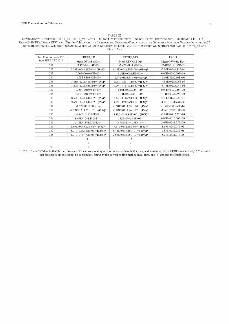
IEEE Transactions on Cybernetics 4

TABLE S2 EXPERIMENTAL RESULTS OF FROFI_FR, FROFI_MO, AND FROFI OVER 25 INDEPENDENT RUNS ON 18 TEST FUNCTIONS WITH 10D FROM IEEE CEC2010

USING 2×105 FES. “MEAN OFV” AND “STD DEV” INDICATE THE AVERAGE AND STANDARD DEVIATION OF THE OBJECTIVE FUNCTION VALUES OBTAINED IN 25 RUNS, RESPECTIVELY. WILCOXON’S RANK SUM TEST AT A 0.05 SIGNIFICANCE LEVEL WAS PERFORMED BETWEEN FROFI AND EACH OF FROFI_FR AND

FROFI_MO.

Test Function with 10D from IEEE CEC2010

FROFI_FR FROFI_MO FROFI Mean OFV±Std Dev Mean OFV±Std Dev Mean OFV±Std Dev

C01 -7.47E-01±1.4E-13≈ -7.47E-01±1.4E-03≈ -7.47E-01±1.35E-03 C02 2.26E+00±1.19E-01－(88%)* 1.10E+00±1.50E+00－(68%)* -2.02E+00±1.41E-01 C03 0.00E+00±0.00E+00≈ 8.52E+00±1.8E+00－ 0.00E+00±0.00E+00 C04 -1.00E-05±0.00E+00≈ -2.97E-01±3.31E-01－(0%)* -1.00E-05±0.00E+00 C05 3.85E+02±1.48E+02－(0%)* 2.25E+02±1.10E+02－(0%)* -4.84E+02±8.09E-07 C06 3.20E+02±1.92E+02－(0%)* 7.79E+01±1.80E+02－(0%)* -5.79E+02±5.04E-04 C07 0.00E+00±0.00E+00≈ 0.00E+00±0.00E+00≈ 0.00E+00±0.00E+00 C08 7.84E+00±4.98E+00≈ 7.34E+00±5.14E+00≈ 7.11E+00±4.79E+00 C09 8.59E+12±4.64E+12－(0%)* 5.44E+11±6.92E+11－(0%)* 2.50E+01±3.92E+01 C10 9.65E+12±6.63E+12－(0%)* 1.29E+12±2.66E+12－(0%)* 4.17E+01±8.69E-06 C11 -1.52E-03±2.00E-18≈ -1.94E+01±4.38E+00－(0%)* -1.52E-03±5.63E-14 C12 -8.23E+13±1.52E+02－(60%)* -1.82E+03±2.86E+02－(0%)* -3.84E+02±2.17E+02 C13 -6.84E+01±2.90E-09≈ -5.81E+01±9.06E+00－(36%)* -6.84E+01±2.52E-09 C14 9.45E+10±1.18E+11－ 1.85E+00±5.46E+00－ 0.00E+00±0.00E+00 C15 3.12E+13±1.72E+13－ 3.71E+11±4.29E+11－ 3.09E+00±1.37E+00 C16 1.05E+00±3.03E-02－(64%)* 7.61E-01±2.66E-01－(28%)* 1.19E-02±2.07E-02 C17 5.07E+02±2.42E+02－(52%)* 8.44E+01±7.18E+01－(40%)* 7.83E-02±2.25E-01 C18 1.01E+04±4.79E+03－(92%)* 2.59E+03±1.98E+03－(44%)* 5.23E-26±1.71E-25 － 11 15 ＋ 0 0 ≈ 7 3

“－”, “＋”, and “≈” denote that the performance of the corresponding method is worse than, better than, and similar to that of FROFI, respectively. “*” denotes that feasible solutions cannot be consistently found by the corresponding method in all runs, and (#) denotes the feasible rate.

IEEE Transactions on Cybernetics 5

TABLE S3 EXPERIMENTAL RESULTS OF FROFI_FR, FROFI_MO, AND FROFI OVER 25 INDEPENDENT RUNS ON 18 TEST FUNCTIONS WITH 30D FROM IEEE CEC2010

USING 6×105 FES. “MEAN OFV” AND “STD DEV” INDICATE THE AVERAGE AND STANDARD DEVIATION OF THE OBJECTIVE FUNCTION VALUES OBTAINED IN 25 RUNS, RESPECTIVELY. WILCOXON’S RANK SUM TEST AT A 0.05 SIGNIFICANCE LEVEL WAS PERFORMED BETWEEN FROFI AND EACH OF FROFI_FR AND

FROFI_MO.

Test Function with 30D from IEEE CEC2010

FROFI_FR FROFI_MO FROFI Mean OFV±Std Dev Mean OFV±Std Dev Mean OFV±Std Dev

C01 -8.21E-01±1.5E-03≈ -8.21E-01±1.69E-03≈ -8.21E-01±2.36E-03 C02 3.40E+00±8.15E-01－ 2.65E+00±6.07E-01－ -2.00E+00±4.35E-02 C03 1.89E+12±7.45E+12－ 2.87E+01±3.02E-04－(96%)* 2.87E+01±6.24E-08 C04 2.60E-02±1.30E-02－ -6.57E-01±1.11E-01－(0%)* -3.33E-06±4.13E-10 C05 5.30E+02±5.09E+01－(0%)* 4.10E+02±8.51E+01－(0%)* -4.81E+02±2.84E+00 C06 5.57E+02±4.25E+01－(0%)* 4.25E+02±7.66E+01－(0%)* -5.29E+02±5.71E-01 C07 1.60E+00±7.97E-01－ 0.00E+00±0.00E+00≈ 0.00E+00±0.00E+00 C08 3.67E+00±1.84E+01－ 5.57E-30±2.79E-29－ 0.00E+00±0.00E+00 C09 3.83E+13±1.10E+13－(4%)* 1.02E+13±5.24E+12－(0%)* 4.30E+01±3.27E+01 C10 3.23E+13±1.17E+12－(8%)* 1.11E+13±6.95E+12－(4%)* 3.13E+01±8.22E-02 C11 -3.92E-04±2.64E-06≈ -1.40E+01±3.00E+00－(0%)* -3.92E-04±2.64E-06 C12 6.37E+01±2.81E+02－(28%)* -5.46E+03±7.19E+02－(0%)* -1.99E-01±1.42E-06 C13 -6.23E+01±1.50E+00－ -7.48E+01±8.66E+00－(0%)* -6.83E+01±1.95E-01 C14 3.56E+07±1.23E+08－ 1.47E+01±4.84E+00－ 9.80E-29±4.90E-28 C15 1.66E+14±4.79E+13－ 2.74E+13±1.22E+13－ 2.16E+01±8.03E-05 C16 1.18E+00±3.46E-02－(40%)* 1.06E+00±2.57E-02－(32%)* 0.00E+00±0.00E+00 C17 1.76E+03±4.89E+02－(76%)* 6.63E+02±2.83E+02－(44%)* 1.59E-01±3.82E-01 C18 2.87E+04±5.26E+03－ 1.44E+04±6.15E+03－(92%)* 4.87E-01±1.25E+00 － 16 16 ＋ 0 0 ≈ 2 2

“－”, “＋”, and “≈” denote that the performance of the corresponding method is worse than, better than, and similar to that of FROFI, respectively. “*” denotes that feasible solutions cannot be consistently found by the corresponding method in all runs, and (#) denotes the feasible rate.

IEEE Transactions on Cybernetics 6

TABLE S4 COMPARISON OF FROFI WITH RESPECT TO εDE [47], APF-GA [69], (μ+λ)-CDE [31], DYHF [56], AND CMODE [57] IN TERMS OF THE SUCCESS RATE. IN ALL

THE EXPERIMENTS, 25 INDEPENDENT RUNS WERE IMPLEMENTED ON 24 TEST FUNCTIONS FROM IEEE CEC2006 USING 5×105 FES.

Test Function from IEEE CEC2006

Success Rate εDE APF-GA (μ+λ)-CDE DyHF CMODE FROFI

g01 100% 100% 100% 100% 100% 100% g02 100% 60% 96% 100% 100% 100% g03 100% 100% 100% 100% 100% 100% g04 100% 100% 100% 100% 100% 100% g05 100% 55% 100% 100% 100% 100% g06 100% 100% 100% 100% 100% 100% g07 100% 100% 100% 100% 100% 100% g08 100% 100% 100% 100% 100% 100% g09 100% 100% 100% 100% 100% 100% g10 100% 55% 100% 100% 100% 100% g11 100% 100% 100% 100% 100% 100% g12 100% 100% 100% 100% 100% 100% g13 100% 70% 100% 100% 100% 100% g14 100% 64% 100% 100% 100% 100% g15 100% 100% 100% 100% 100% 100% g16 100% 80% 100% 100% 100% 100% g17 100% 36% 100% 100% 100% 100% g18 100% 96% 100% 100% 100% 100% g19 100% 100% 100% 100% 100% 100% g20 0% 0% 100% 0% 100% 100% g21 100% 0% 92% 100% 80% 100% g22 0% 0% 0% 0% 0% 0% g23 100% 0% 100% 100% 100% 100% g24 100% 100% 100% 100% 100% 100%

Mean 91.67% 71.50% 95.33% 91.67% 95.00% 95.83%

IEEE Transactions on Cybernetics 7

TABLE S5 COMPARISON OF FROFI WITH RESPECT TOεDE [47], APF-GA [69], (μ+λ)-CDE [31], DYHF [56], AND CMODE [57] IN TERMS OF THE SUCCESS PERFORMANCE.

IN ALL THE EXPERIMENTS, 25 INDEPENDENT RUNS WERE IMPLEMENTED ON 24 TEST FUNCTIONS FROM IEEE CEC2006 USING 5×105 FES.

Test Function from IEEE CEC2006

Success Performance εDE APF-GA (μ+λ)-CDE DyHF CMODE FROFI

g01 5.9E+04 4.2E+05 8.9E+04 6.9E+04 1.2E+05 3.8E+04 g02 1.5E+05 6.8E+05 2.7E+05 1.1E+05 1.9E+05 8.5E+04 g03 8.9E+04 2.3E+05 1.1E+05 4.3E+04 7.5E+04 6.3E+04 g04 2.6E+04 2.6E+05 3.0E+04 4.0E+04 7.3E+04 2.5E+04 g05 9.7E+04 5.7E+05 1.6E+05 4.7E+04 2.9E+04 3.1E+04 g06 7.4E+03 2.0E+05 1.1E+04 3.8E+04 3.5E+04 1.5E+04 g07 7.4E+04 2.2E+05 1.4E+05 9.4E+04 1.6E+05 7.2E+04 g08 1.1E+03 5.7E+04 2.0E+03 1.2E+03 5.9E+03 2.4E+03 g09 2.3E+04 5.3E+04 4.0E+04 4.1E+04 7.1E+04 3.2E+04 g10 1.1E+05 2.9E+05 1.8E+05 1.4E+05 1.8E+05 1.0E+05 g11 1.6E+04 2.2E+05 7.9E+04 5.8E+03 6.0E+03 1.2E+04 g12 4.1E+03 1.1E+05 4.9E+03 3.0E+03 5.0E+03 3.5E+03 g13 3.5E+04 1.1E+05 1.4E+05 3.2E+04 3.1E+04 4.1E+04 g14 1.1E+05 2.4E+05 1.7E+05 6.5E+04 1.1E+05 6.6E+04 g15 8.4E+04 1.8E+04 1.3E+05 2.3E+04 1.3E+04 1.9E+04 g16 1.3E+04 4.9E+04 1.9E+04 3.0E+04 2.9E+04 1.8E+04 g17 9.9E+04 3.2E+05 1.8E+05 2.1E+05 1.4E+05 1.3E+05 g18 5.9E+04 2.2E+05 2.1E+05 8.9E+04 1.1E+05 9.6E+04 g19 3.5E+05 2.6E+04 2.6E+05 1.1E+05 2.5E+05 1.2E+05 g20 NA NA 1.4E+05 NA 4.4E+05 4.7E+05 g21 1.4E+05 NA 2.1E+05 1.0E+05 1.3E+05 9.4E+04 g22 NA NA NA NA NA NA g23 2.0E+05 NA 2.6E+05 1.6E+05 2.4E+05 1.7E+05 g24 3.0E+03 1.9E+05 5.0E+03 1.4E+04 2.2E+04 5.7E+03

IEEE Transactions on Cybernetics 8

TABLE S6 EXPERIMENTAL RESULTS OF εDEAG [51], SRS-εDEAG [50], ECHT-DE [72], AIS-IRP [40], AND FROFI OVER 25 INDEPENDENT RUNS ON 18 TEST FUNCTIONS WITH 10D FROM IEEE CEC2010 USING 2×105 FES. “MEAN OFV” AND “STD DEV” INDICATE THE AVERAGE AND STANDARD DEVIATION OF THE OBJECTIVE

FUNCTION VALUES OBTAINED IN 25 RUNS, RESPECTIVELY. t -TEST AT A 0.05 SIGNIFICANCE LEVEL WAS PERFORMED BETWEEN FROFI AND EACH OF εDEAG, SRS-εDEAG, ECHT-DE, AND AIS-IRP.

Test Function with 10D from IEEE CEC2010

εDEag SRS-εDEag ECHT-DE AIS-IRP FROFI

Mean OFV±Std Dev Mean OFV±Std Dev Mean OFV±Std Dev Mean OFV±Std Dev Mean OFV±Std Dev C01 -7.47E-01±1.32E-03≈ -7.47E-01±2.82E-03≈ -7.47E-01±1.40E-03≈ -7.47E-01±1.30E-03≈ -7.47E-01±1.35E-03 C02 -2.26E+00±2.39E-02＋ -2.27E+00±1.28E-02＋ -2.27E+00±6.70E-03＋ -2.27E+00±2.00E-03＋ -2.02E+00±1.41E-01 C03 0.00E+00±0.00E+00≈ 0.00E+00±0.00E+00≈ 0.00E+00±0.00E+00≈ 3.75E-09±4.81E-04－ 0.00E+00±0.00E+00 C04 -9.92E-06±1.55E-07－ -9.99E-06±1.60E-10－ -1.00E-05±0.00E+00≈ -9.97E-06±4.28E-03≈ -1.00E-05±0.00E+00 C05 -4.84E+02±3.89E-13≈ -4.84E+02±6.25E-13≈ -4.11E+02±7.63E+01－ -4.80E+02±6.30E+00－ -4.84E+02±8.09E-07 C06 -5.79E+02±3.63E-03－ -5.79E+02±9.07E-04≈ -5.62E+02±4.51E+01－ -5.80E+02±7.30E-08＋ -5.79E+02±5.04E-04 C07 0.00E+00±0.00E+00≈ 0.00E+00±0.00E+00≈ 1.33E-01±7.28E-01－ 1.17E-08±2.70E+00－ 0.00E+00±0.00E+00 C08 6.73E+00±5.56E+00≈ 8.39E+00±4.49E+00≈ 6.16E+00±6.45E+00≈ 4.09E+00±1.46E+00＋ 7.11E+00±4.79E+00 C09 0.00E+00±0.00E+00＋ 2.93E+01±1.99E+01≈ 1.47E-01±8.05E-01＋ 2.70E+01±7.50E+01≈ 2.50E+01±3.92E+01 C10 0.00E+00±0.00E+00＋ 4.80E+01±3.29E+01≈ 1.71E+00±7.66E+00＋ 1.62E+03±5.00E+02－ 4.17E+01±8.69E-06 C11 -1.52E-03±6.34E-11≈ -1.52E-03±6.02E-11≈ -4.40E-03±1.57E-02－* -9.20E-04±8.23E-04－ -1.52E-03±5.63E-14 C12 -3.37E+02±1.78E+02－ -4.70E+02±1.42E+02＋ -1.72E+02±2.21E+02－* -4.36E+02±6.02E+01≈ -3.84E+02±2.17E+02 C13 -6.84E+01±1.03E-06≈ -6.80E+01±1.33E+00－ -6.51E+01±2.38E+00－ -6.79E+01±3.11E-01－ -6.84E+01±2.52E-09 C14 0.00E+00±0.00E+00≈ 0.00E+00±0.00E+00≈ 7.02E+05±3.19E+06－ 1.22E-04±2.90E-08－ 0.00E+00±0.00E+00 C15 1.80E-01±8.81E-01＋ 2.21E+01±1.05E+02－ 2.34E+13±5.30E+13－ 5.19E-09±1.10E-08＋ 3.09E+00±1.37E+00 C16 3.70E-01±3.71E-01－ 2.34E-02±2.64E-02≈ 3.93E-02±4.28E-02－ 9.96E-18±6.27E-15＋ 1.19E-02±2.07E-02 C17 1.25E-01±1.94E-01－ 4.15E-02±1.24E-01≈ 1.12E-01±3.32E-01－ 2.93E+00±2.29E+00－ 7.83E-02±2.25E-01 C18 9.68E-19±1.81E-18－ 5.79E-17±2.24E-16－ 0.00E+00±0.00E+00＋ 1.66E+00±1.27E+00－ 5.23E-26±1.71E-25 － 6 4 10 9 ＋ 4 2 4 5 ≈ 8 12 4 4

“－”, “＋”, and “≈” denote that the performance of the corresponding method is worse than, better than, and similar to that of FROFI, respectively. “*” denotes that feasible solutions cannot be consistently found by the corresponding method in all runs.

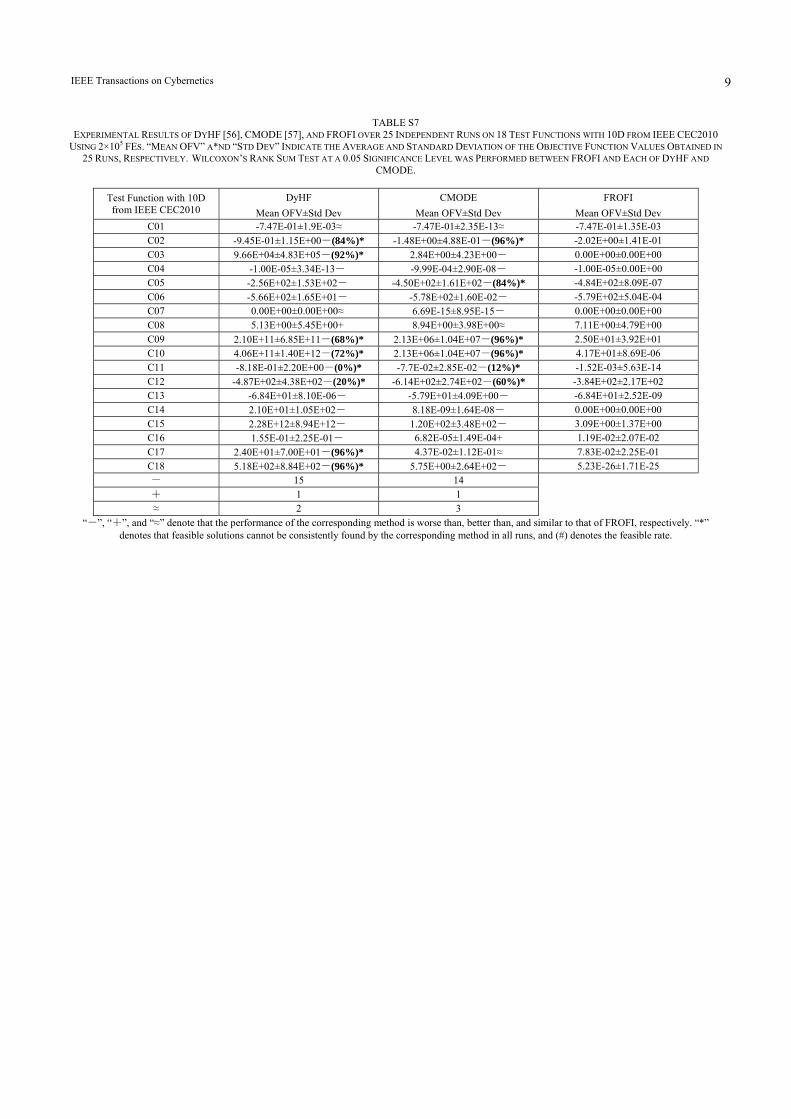
IEEE Transactions on Cybernetics 9

TABLE S7 EXPERIMENTAL RESULTS OF DYHF [56], CMODE [57], AND FROFI OVER 25 INDEPENDENT RUNS ON 18 TEST FUNCTIONS WITH 10D FROM IEEE CEC2010

USING 2×105 FES. “MEAN OFV” A*ND “STD DEV” INDICATE THE AVERAGE AND STANDARD DEVIATION OF THE OBJECTIVE FUNCTION VALUES OBTAINED IN 25 RUNS, RESPECTIVELY. WILCOXON’S RANK SUM TEST AT A 0.05 SIGNIFICANCE LEVEL WAS PERFORMED BETWEEN FROFI AND EACH OF DYHF AND

CMODE.

Test Function with 10D from IEEE CEC2010

DyHF CMODE FROFI Mean OFV±Std Dev Mean OFV±Std Dev Mean OFV±Std Dev

C01 -7.47E-01±1.9E-03≈ -7.47E-01±2.35E-13≈ -7.47E-01±1.35E-03 C02 -9.45E-01±1.15E+00－(84%)* -1.48E+00±4.88E-01－(96%)* -2.02E+00±1.41E-01 C03 9.66E+04±4.83E+05－(92%)* 2.84E+00±4.23E+00－ 0.00E+00±0.00E+00 C04 -1.00E-05±3.34E-13－ -9.99E-04±2.90E-08－ -1.00E-05±0.00E+00 C05 -2.56E+02±1.53E+02－ -4.50E+02±1.61E+02－(84%)* -4.84E+02±8.09E-07 C06 -5.66E+02±1.65E+01－ -5.78E+02±1.60E-02－ -5.79E+02±5.04E-04 C07 0.00E+00±0.00E+00≈ 6.69E-15±8.95E-15－ 0.00E+00±0.00E+00 C08 5.13E+00±5.45E+00+ 8.94E+00±3.98E+00≈ 7.11E+00±4.79E+00 C09 2.10E+11±6.85E+11－(68%)* 2.13E+06±1.04E+07－(96%)* 2.50E+01±3.92E+01 C10 4.06E+11±1.40E+12－(72%)* 2.13E+06±1.04E+07－(96%)* 4.17E+01±8.69E-06 C11 -8.18E-01±2.20E+00－(0%)* -7.7E-02±2.85E-02－(12%)* -1.52E-03±5.63E-14 C12 -4.87E+02±4.38E+02－(20%)* -6.14E+02±2.74E+02－(60%)* -3.84E+02±2.17E+02 C13 -6.84E+01±8.10E-06－ -5.79E+01±4.09E+00－ -6.84E+01±2.52E-09 C14 2.10E+01±1.05E+02－ 8.18E-09±1.64E-08－ 0.00E+00±0.00E+00 C15 2.28E+12±8.94E+12－ 1.20E+02±3.48E+02－ 3.09E+00±1.37E+00 C16 1.55E-01±2.25E-01－ 6.82E-05±1.49E-04+ 1.19E-02±2.07E-02 C17 2.40E+01±7.00E+01－(96%)* 4.37E-02±1.12E-01≈ 7.83E-02±2.25E-01 C18 5.18E+02±8.84E+02－(96%)* 5.75E+00±2.64E+02－ 5.23E-26±1.71E-25 － 15 14 ＋ 1 1 ≈ 2 3

“－”, “＋”, and “≈” denote that the performance of the corresponding method is worse than, better than, and similar to that of FROFI, respectively. “*” denotes that feasible solutions cannot be consistently found by the corresponding method in all runs, and (#) denotes the feasible rate.

IEEE Transactions on Cybernetics 10

TABLE S8 EXPERIMENTAL RESULTS OFεDEAG [51], SRS-εDEAG [50], ECHT-DE [72], AIS-IRP [40], AND FROFI OVER 25 INDEPENDENT RUNS ON 18 TEST FUNCTIONS WITH 30D FROM IEEE CEC2010 USING 6×105 FES. “MEAN OFV” AND “STD DEV” INDICATE THE AVERAGE AND STANDARD DEVIATION OF THE OBJECTIVE

FUNCTION VALUES OBTAINED IN 25 RUNS, RESPECTIVELY. t -TEST AT A 0.05 SIGNIFICANCE LEVEL WAS PERFORMED BETWEEN FROFI AND EACH OF εDEAG, SRS-εDEAG, ECHT-DE, AND AIS-IRP.

Test Function with 30D from IEEE CEC2010

εDEag SRS-εDEag ECHT-DE AIS-IRP FROFI

Mean OFV±Std Dev Mean OFV±Std Dev Mean OFV±Std Dev Mean OFV±Std Dev Mean OFV±Std Dev C01 -8.21E-01±7.10E-04≈ -8.21E-01±6.10E-04≈ -8.00E-01±1.79E-02－ -8.20E-01±3.25E-04≈ -8.21E-01±2.36E-03 C02 -2.15E+00±1.20E-02＋ -2.19E+00±8.88E-03＋ -1.99E+00±2.10E-01－ -2.21E+00±2.84E-03＋ -2.00E+00±4.35E-02 C03 2.88E+01±8.05E-01－ 2.87E+01±2.80E-07≈ 9.89E+01±6.26E+01－ 6.68E+01±4.26E+02－ 2.87E+01±6.24E-08 C04 8.16E-03±3.07E-03－ 5.70E-03±1.84E-03－ -1.03E-06±9.01E-03－ 1.98E-03±1.61E-03－ -3.33E-06±4.13E-10 C05 -4.50E+02±2.90E+00－ -4.63E+02±3.37E+00－ -1.06E+02±1.67E+02－ -4.36E+02±2.51E+01－ -4.81E+02±2.84E+00 C06 -5.28E+02±4.75E-01－ -5.29E+02±2.54E-01≈ -1.38E+02±9.89E+01－ -4.54E+02±4.79E+01－ -5.29E+02±5.71E-01 C07 2.60E-15±1.23E-15－ 2.70E-15±1.61E-15－ 1.33E-01±7.28E-01－ 1.07E+00±1.61E+00－ 0.00E+00±0.00E+00 C08 7.83E-14±4.86E-14－ 4.90E-14±3.09E-14－ 3.36E+01±1.11E+02－ 1.65E+00±6.41E-01－ 0.00E+00±0.00E+00 C09 1.07E+01±2.82E+01＋ 2.43E+00±1.20E+01＋ 4.24E+01±1.38E+02≈ 1.57E+00±1.96E+00＋ 4.30E+01±3.27E+01 C10 3.33E+01±4.55E-01－ 3.29E+01±4.74E-01－ 5.34E+01±8.83E+01≈ 1.78E+01±1.88E+01＋ 3.13E+01±8.22E-02 C11 -2.86E-04±2.71E-05－ -2.99E-04±3.32E-05－ 2.60E-03±6.00E-03－* -1.58E-04±4.67E-05－ -3.92E-04±2.64E-06 C12 3.56E+02±2.89E+02－* 2.13E+02±2.71E+02－* -2.51E+01±1.37E+02－* 4.29E-06±4.52E-04－ -1.99E-01±1.42E-06 C13 -6.54E+01±5.73E-01－ -6.59E+01±6.18E-01－ -6.46E+01±1.67E+00－ -6.62E+01±2.27E-01－ -6.83E+01±1.95E-01 C14 3.09E-13±5.61E-13－ 1.04E-13±8.24E-14－ 1.24E+05±6.77E+05－ 8.68E-07±3.14E-07－ 9.80E-29±4.90E-28 C15 2.16E+01±1.10E-04≈ 2.16E+01±6.24E-05≈ 1.94E+11±4.35E+11－ 3.41E+01±3.82E+01－ 2.16E+01±8.03E-05 C16 2.17E-21±1.06E-20－ 0.00E+00±0.00E+00≈ 0.00E+00±0.00E+00≈ 8.21E-02±1.12E-01－ 0.00E+00±0.00E+00 C17 6.33E+00±4.99E+00－ 1.17E-01±7.77E-01≈ 2.75E-01±3.78E-01－ 3.61E+00±2.54E+00－ 1.59E-01±3.82E-01 C18 8.75E+01±1.66E+02－ 3.95E+01±6.23E+01－ 0.00E+00±0.00E+00＋ 4.02E+01±1.80E+01－ 4.87E-01±1.25E+00 － 14 10 14 14 ＋ 2 2 1 3 ≈ 2 6 3 1

“－”, “＋”, and “≈” denote that the performance of the corresponding method is worse than, better than, and similar to that of FROFI, respectively. “*” denotes that feasible solutions cannot be consistently found by the corresponding method in all runs.

IEEE Transactions on Cybernetics 11

TABLE S9 EXPERIMENTAL RESULTS OF DYHF [56], CMODE [57], AND FROFI OVER 25 INDEPENDENT RUNS ON 18 TEST FUNCTIONS WITH 30D FROM IEEE CEC2010 USING 6×105 FES. “MEAN OFV” AND “STD DEV” INDICATE THE AVERAGE AND STANDARD DEVIATION OF THE OBJECTIVE FUNCTION VALUES OBTAINED IN

25 RUNS, RESPECTIVELY. WILCOXON’S RANK SUM TEST AT A 0.05 SIGNIFICANCE LEVEL WAS PERFORMED BETWEEN FROFI AND EACH OF DYHF AND CMODE.

Test Function with 30D from IEEE CEC2010

DyHF CMODE FROFI Mean OFV±Std Dev Mean OFV±Std Dev Mean OFV±Std Dev

C01 -8.21E-01±1.80E-03≈ -8.21E-01±3.3E-03≈ -8.21E-01±2.36E-03 C02 5.74E-01±1.59E+00－(88%)* 9.75E-01±6.25E+01－ -2.00E+00±4.35E-02 C03 3.03E+12±8.18E+12－(0%)* 2.18E+01±1.25E+01≈ 2.87E+01±6.24E-08 C04 8.25E+00±7.15E+00－(0%)* 6.72E-04±4.24E-04－ -3.33E-06±4.13E-10 C05 2.95E+12±8.18E+12－(60%)* 2.77E+02±2.03E+02－(0%)* -4.81E+02±2.84E+00 C06 -2.10E+01±2.91E+02－(88%)* -4.96E+02±2.15E+02－(0%)* -5.29E+02±5.71E-01 C07 1.59E-01±7.97E-01－ 5.24E-05±5.89E-05－ 0.00E+00±0.00E+00 C08 4.72E+00±2.36E+01－ 3.68E-01±2.62E-01－ 0.00E+00±0.00E+00 C09 1.50E+13±1.57E+13－(60%)* 1.72E+13±1.07E+13－(0%)* 4.30E+01±3.27E+01 C10 1.57E+13±1.38E+13－(44%)* 1.60E+13±7.00E+12－(12%)* 3.13E+01±8.22E-02 C11 -1.68E-01±7.04E-01－(0%)* 9.5E-03±9.7E-03－(48%)* -3.92E-04±2.64E-06 C12 -1.59E+01±3.87E+02－(0%)* -3.46E+00±7.35E+02－(84%)* -1.99E-01±1.42E-06 C13 -6.61E+01±1.91E+00－ -3.89E+01±2.17E+00－ -6.83E+01±1.95E-01 C14 2.41E+12±8.94E+12－ 9.31E+00±2.46E+00－ 9.80E-29±4.90E-28 C15 5.49E+13±7.61E+13－ 1.51E+13±8.26E+12－ 2.16E+01±8.03E-05 C16 7.41E-01±1.85E-01－ 6.30E-02±2.72E-02－ 0.00E+00±0.00E+00 C17 6.04E+02±4.92E+02－(76%)* 3.12E+02±2.75E+02－(80%)* 1.59E-01±3.82E-01 C18 1.18E+04±1.31E+04－(76%)* 7.36E+03±3.12E+03－ 4.87E-01±1.25E+00 － 17 16 ＋ 0 0 ≈ 1 2

“－”, “＋”, and “≈” denote that the performance of the corresponding method is worse than, better than, and similar to that of FROFI, respectively. “*” denotes that feasible solutions cannot be consistently found by the corresponding method in all runs, and (#) denotes the feasible rate.

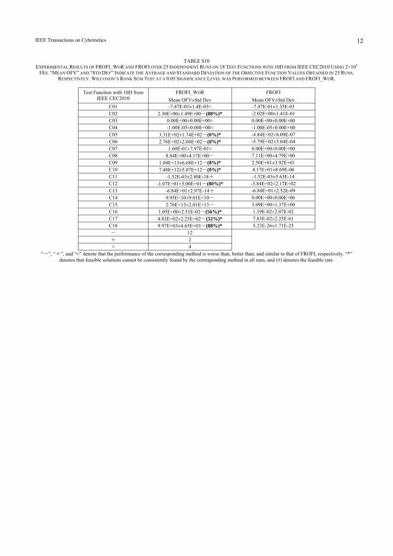
IEEE Transactions on Cybernetics 12

TABLE S10 EXPERIMENTAL RESULTS OF FROFI_WOR AND FROFI OVER 25 INDEPENDENT RUNS ON 18 TEST FUNCTIONS WITH 10D FROM IEEE CEC2010 USING 2×105

FES. “MEAN OFV” AND “STD DEV” INDICATE THE AVERAGE AND STANDARD DEVIATION OF THE OBJECTIVE FUNCTION VALUES OBTAINED IN 25 RUNS, RESPECTIVELY. WILCOXON’S RANK SUM TEST AT A 0.05 SIGNIFICANCE LEVEL WAS PERFORMED BETWEEN FROFI AND FROFI_WOR.

Test Function with 10D from

IEEE CEC2010 FROFI_WOR FROFI

Mean OFV±Std Dev Mean OFV±Std Dev C01 -7.47E-01±1.4E-03≈ -7.47E-01±1.35E-03 C02 2.30E+00±1.49E+00－(88%)* -2.02E+00±1.41E-01 C03 0.00E+00±0.00E+00≈ 0.00E+00±0.00E+00 C04 -1.00E-05±0.00E+00≈ -1.00E-05±0.00E+00 C05 3.31E+02±1.74E+02－(0%)* -4.84E+02±8.09E-07 C06 2.76E+02±2.04E+02－(0%)* -5.79E+02±5.04E-04 C07 1.60E-01±7.97E-01≈ 0.00E+00±0.00E+00 C08 8.84E+00±4.17E+00－ 7.11E+00±4.79E+00 C09 1.04E+13±6.68E+12－(8%)* 2.50E+01±3.92E+01 C10 7.48E+12±5.07E+12－(0%)* 4.17E+01±8.69E-06 C11 -1.52E-03±2.80E-18＋ -1.52E-03±5.63E-14 C12 -1.07E+01±5.00E+01－(80%)* -3.84E+02±2.17E+02 C13 -6.84E+01±2.97E-14＋ -6.84E+01±2.52E-09 C14 9.95E+10±9.01E+10－ 0.00E+00±0.00E+00 C15 2.76E+13±2.01E+13－ 3.09E+00±1.37E+00 C16 1.05E+00±2.51E-02－(56%)* 1.19E-02±2.07E-02 C17 4.83E+02±2.23E+02－(52%)* 7.83E-02±2.25E-01 C18 9.97E+03±4.65E+03－(88%)* 5.23E-26±1.71E-25 － 12 ＋ 2 ≈ 4

“－”, “＋”, and “≈” denote that the performance of the corresponding method is worse than, better than, and similar to that of FROFI, respectively. “*” denotes that feasible solutions cannot be consistently found by the corresponding method in all runs, and (#) denotes the feasible rate.

IEEE Transactions on Cybernetics 13

TABLE S11 EXPERIMENTAL RESULTS OF FROFI_WOR AND FROFI OVER 25 INDEPENDENT RUNS ON 18 TEST FUNCTIONS WITH 30D FROM IEEE CEC2010 USING 6×105

FES. “MEAN OFV” AND “STD DEV” INDICATE THE AVERAGE AND STANDARD DEVIATION OF THE OBJECTIVE FUNCTION VALUES OBTAINED IN 25 RUNS, RESPECTIVELY. WILCOXON’S RANK SUM TEST AT A 0.05 SIGNIFICANCE LEVEL WAS PERFORMED BETWEEN FROFI AND FROFI_WOR.

Test Function with 30D from

IEEE CEC2010 FROFI_WOR FROFI

Mean OFV±Std Dev Mean OFV±Std Dev C01 -8.20E-01±2.1E-03≈ -8.21E-01±2.36E-03 C02 3.22E+00±5.32E-01－ -2.00E+00±4.35E-02 C03 3.26E+11±1.21E+12－ 2.87E+01±6.24E-08 C04 -3.31E-06±6.87E-08－ -3.33E-06±4.13E-10 C05 5.06E+02±8.05E+01－(0%)* -4.81E+02±2.84E+00 C06 5.40E+02±6.19E+01－(0%)* -5.29E+02±5.71E-01 C07 0.00E+00±0.00E+00≈ 0.00E+00±0.00E+00 C08 1.60E-01±7.97E-01－ 0.00E+00±0.00E+00 C09 3.40E+13±1.04E+13－(0%)* 4.30E+01±3.27E+01 C10 4.32E+13±1.40E+13－(4%)* 3.13E+01±8.22E-02 C11 -3.92E-04±4.78E-09＋ -3.92E-04±2.64E-06 C12 -3.23E+01±1.95E+02－(48%)* -1.99E-01±1.42E-06 C13 -6.25E+01±1.75E+00－ -6.83E+01±1.95E-01 C14 2.65E+08±1.01E+09－ 9.80E-29±4.90E-28 C15 1.63E+14±5.43E+13－ 2.16E+01±8.03E-05 C16 1.14E+00±4.01E-02－(44%)* 0.00E+00±0.00E+00 C17 1.61E+03±5.05E+02－(88%)* 1.59E-01±3.82E-01 C18 2.92E+04±6.16E+03－ 4.87E-01±1.25E+00 － 15 ＋ 1 ≈ 2

“－”, “＋”, and “≈” denote that the performance of the corresponding method is worse than, better than, and similar to that of FROFI, respectively. “*” denotes that feasible solutions cannot be consistently found by the corresponding method in all runs, and (#) denotes the feasible rate.

IEEE Transactions on Cybernetics 14

TABLE S12 EXPERIMENTAL RESULTS OF FROFI_13, FROFI_14, FROFI_15, FROFI_16, AND FROFI_17 OVER 25 INDEPENDENT RUNS ON 18 TEST FUNCTIONS WITH 30D FROM IEEE CEC2010 USING 6×105 FES. “MEAN OFV” AND “STD DEV” INDICATE THE AVERAGE AND STANDARD DEVIATION OF THE OBJECTIVE FUNCTION VALUES OBTAINED IN 25

RUNS, RESPECTIVELY.

Test Function with 30D from IEEE CEC2010

FROFI_13 FROFI_14 FROFI_15 FROFI_16 FROFI_17 Mean OFV±Std Dev Mean OFV±Std Dev Mean OFV±Std Dev Mean OFV±Std Dev Mean OFV±Std Dev

C01 -8.20E-01±2.29E-03 -8.20E-01±2.25E-03 -8.21E-01±2.36E-03 -8.20E-01±2.39E-03 -8.20E-01±1.73E-03 C02 -1.99E+00±4.79E-02 -1.99E+00±4.34E-02 -2.00E+00±4.35E-02 -2.01E+00±3.80E-02 -2.00E+00±4.13E-02 C03 2.87E+01±2.55E-08 2.87E+01±3.99E-08 2.87E+01±6.24E-08 2.75E+01±5.73E+00 2.87E+01±5.74E-08 C04 -3.33E-06±8.53E-11 -3.33E-06±5.35E-10 -3.33E-06±4.13E-10 -3.33E-06±1.88E-10 -3.33E-06±8.2E-11 C05 -4.81E+02±1.70E+00 -4.81E+02±1.10E+00 -4.81E+02±2.84E+00 -4.81E+02±1.33E+00 -4.81E+02±1.58E+00 C06 -5.27E+02±1.20E+00 -5.28E+02±8.70E-01 -5.29E+02±5.71E-01 -5.28E+02±7.85E-01 -5.28E+02±7.60E-01 C07 0.00E+00±0.00E+00 1.59E-01±7.97E-01 0.00E+00±0.00E+00 0.00E+00±0.00E+00 0.00E+00±0.00E+00 C08 3.67E+00±1.84E+01 8.49E+00±2.94E+01 0.00E+00±0.00E+00 0.00E+00±0.00E+00 3.67E+00±1.84E+01 C09 5.68E+01±1.12E+02 5.70E+01±2.84E+01 4.30E+01±3.27E+01 3.67E+01±4.23E+01 4.14E+01±3.80E+01 C10 3.17E+01±1.47E+00 3.14E+01±9.02E-01 3.13E+01±8.22E-02 3.13E+01±2.64E-02 3.13E+01±1.85E-02 C11 -3.92E-04±1.65E-06 -3.92E-04±1.18E-08 -3.92E-04±2.64E-06 -3.92E-04±1.77E-07 -3.92E-04±2.44E-07

C12 1.71E-01±1.33E+00 (84%)*

-1.17E+01±5.88E+01 (88%)* -1.99E-01±1.42E-06 -7.92E-01±3.35E+00

(92%)* -5.08E+00±2.52E+01

(92%)* C13 -6.82E+01±4.86E-01 -6.80E+01±6.59E-01 -6.83E+01±1.95E-01 -6.82E+01±4.01E-01 -6.83E+01±3.73E-01 C14 1.59E-01±7.97E-01 0.00E+00±0.00E+00 9.80E-29±4.90E-28 0.00E+00±0.00E+00 0.00E+00±0.00E+00 C15 2.16E+01±3.53E-05 2.16E+01±5.61E-05 2.16E+01±8.03E-05 2.16E+01±6.87E-05 2.16E+01±1.02E-04 C16 0.00E+00±0.00E+00 6.78E-04±3.39E-03 0.00E+00±0.00E+00 5.10E-03±4.42E-01 2.49E-03±1.24E-02 C17 1.47E-01±2.40E-01 2.99E-01±3.94E-01 1.59E-01±3.82E-01 2.25E-01±4.42E-01 2.19E-01±4.57E-01 C18 1.90E+00±6.08E+00 9.68E-01±2.33E+00 4.87E-01±1.25E+00 6.86E-01±1.73E+00 1.12E+00±3.55E+00

“*” denotes that feasible solutions cannot be consistently found by the corresponding method in all runs, and (#) denotes the feasible rate.