IEEE Transactions on Cybernetics 1

Abstract—In the field of evolutionary computation, there has

been a growing interest in applying evolutionary algorithms to solve multimodal optimization problems (MMOPs). Due to the fact that an MMOP involves multiple optimal solutions, many niching methods have been suggested and incorporated into evolutionary algorithms for locating such optimal solutions in a single run. In this paper, we propose a novel transformation technique based on multiobjective optimization for MMOPs, called MOMMOP. MOMMOP transforms an MMOP into a multiobjective optimization problem with two conflicting objectives. After the above transformation, all the optimal solutions of an MMOP become the Pareto optimal solutions of the transformed problem. Thus, multiobjective evolutionary algorithms can be readily applied to find a set of representative Pareto optimal solutions of the transformed problem, and as a result, multiple optimal solutions of the original MMOP could also be simultaneously located in a single run. In principle, MOMMOP is an implicit niching method. In this paper, we also discuss two issues in MOMMOP and introduce two new comparison criteria. MOMMOP has been used to solve 20 multimodal benchmark test functions, after combining with nondominated sorting and differential evolution. Systematic experiments have indicated that MOMMOP outperforms a number of methods for multimodal optimization, including four recent methods at the 2013 IEEE Congress on Evolutionary Computation, four state-of-the-art single-objective optimization based methods, and two well-known multiobjective optimization based approaches.

Index Terms—Multimodal optimization problems, multiple

optimal solutions, transformation technique, multiobjective optimization, evolutionary algorithms.

Manuscript received October 16, 2013; revised May 10, 2014 and June 24,

2014; Accepted July 2, 2014. This work was supported in part by the National Natural Science Foundation of China under Grant 61273314, Grant 51175519, and Grant 61175064, in part by the Hong Kong Scholars Program, in part by the China Postdoctoral Science Foundation under Grant 2013M530359, in part by RGC of Hong Kong (CityU: 116212), and in part by the Program for New Century Excellent Talents in University under Grant NCET-13-0596. (Corresponding Author: Wu Song)

Y. Wang is with the School of Information Science and Engineering, Central South University, Changsha 410083, China, and also with the Department of Systems Engineering and Engineering Management, City University of Hong Kong, Hong Kong. (e-mail: ywang@csu.edu.cn)

H.-X. Li is with the Department of Systems Engineering and Engineering Management, City University of Hong Kong, Hong Kong, and the State Key Laboratory of High Performance Complex Manufacturing, Central South University, Changsha 410083, China. (e-mail: mehxli@cityu.edu.hk)

G. G. Yen is with the School of Electrical and Computer Engineering, Oklahoma State University, Stillwater, OK 74078 USA. (e-mail: gyen@ okstate.edu)

W. Song is with the College of Electronics and Information Engineering, QiongZhou University, Sanya 572022, China.

I. INTRODUCTION Many optimization problems in real-world applications

exhibit multimodal property [1], [2], that is, multiple optimal solutions coexist. This kind of optimization problems is considered to be multimodal optimization problems (MMOPs). MMOPs have the same formulation as single-objective optimization problems and can be mathematically expressed as follows:

maximize/minimize ( )f x (1) where 1( , , )Dx x x S= ∈… is the decision vector, i i iL x U≤ ≤ ( {1, , })i D∈ … is the ith decision variable, iL and iU are the lower and upper bounds of ix , respectively, D is the number of decision variables, ( )f x is the objective function, and S is the decision space defined as

1

[ , ]D

i ii

S L U=

= ∏ (2)

Evolutionary algorithms (EAs) are a class of population based intelligent optimization methods. During the past four decades, EAs have been widely applied to solve MMOPs [3]. For an MMOP, it is desirable to maintain all the optimal solutions in a single run, and as a result, a user can choose one final solution to satisfy his/her demands. However, due to genetic drift [4], EAs are easy to lose the diversity of the population and tend to converge toward one of the optimal solutions during the evolution. In order to achieve the simultaneous locating of multiple optimal solutions of MMOPs, a variety of niching methods targeted at EAs have been developed. The preselection method suggested by Cavicchio [5] in 1970 is the first implementation of niching methods. Currently, the popular niching methods include clearing [6], fitness sharing [7], crowding [8], [9], [10], restricted tournament selection [11], speciation [12], etc. In addition, niching methods have also been embedded into numerous EA paradigms, such as genetic algorithm [13], artificial immune system [14], particle swarm optimization [15], differential evolution [16], evolution strategy [17], and firefly algorithm [18], to solve MMOPs.

The similarity between MMOPs and multiobjective optimization problems (MOPs) is that both of them involve multiple optimal solutions. Recently, several attempts have been made to solve MMOPs by taking advantage of multiobjective optimization concepts [19], [20], [21]. This kind of methods usually transforms an MMOP into a MOP with two objectives (i.e., a biobjective optimization problem),

Yong Wang, Member, IEEE, Han-Xiong Li, Fellow, IEEE, Gary G. Yen, Fellow, IEEE, and Wu Song

MOMMOP: Multiobjective Optimization for Locating Multiple Optimal Solutions of

Multimodal Optimization Problems

IEEE Transactions on Cybernetics 2

in which the first objective is the multimodal function itself, and the second objective is constructed based on the gradient information [19], [20] or the distance information [21] of the population. After the above transformation, it is expected that multiple optimal solutions of an MMOP can be obtained by using multiobjective EAs (MOEAs) [22], [23], [24] to deal with the transformed problem. However, it is necessary to note that the conflicting objectives are the prerequisite for the coexistence of multiple Pareto optimal solutions in MOPs. Although this kind of methods can alleviate the drawbacks of the existing niching methods (e.g., some problem-dependent niching parameters) to a certain degree, it cannot guarantee that the two objectives in the transformed problem totally conflict with each other. The above situation implies that optimizing the transformed problem by MOEAs may fail to concurrently locate multiple optimal solutions of the original MMOP in a single run. Moreover, under this condition, the relationship between the optimal solutions of the original MMOP and the Pareto optimal solutions of the transformed problem is difficult to verify theoretically.

Based on the above consideration, in this paper we propose a novel transformation technique based on multiobjective optimization for MMOPs, called MOMMOP. MOMMOP also transforms an MMOP into a biobjective optimization problem; however, unlike the previous work, the two objectives in MOMMOP totally conflict with each other. Moreover, it can be proven that all the optimal solutions of an MMOP are the Pareto optimal solutions of the transformed problem. In principle, MOMMOP is an implicit niching method. After the above transformation, MOEAs are able to approximate the Pareto optimal solutions of the transformed problem in a single run, and as a result, multiple optimal solutions of an MMOP could also be obtained. In addition, two issues in MOMMOP have been identified, and two new comparison criteria have been designed to remedy these two issues. The performance of MOMMOP has been evaluated on 20 multimodal benchmark test functions developed for the special session and competition on niching methods for multimodal function optimization of the 2013 IEEE Congress on Evolutionary Computation (IEEE CEC2013) [25]. The experimental results suggest that MOMMOP performs better than a variety of methods for multimodal optimization.

The rest of this paper is organized as follows. Section II introduces MOPs and differential evolution [26]. Section III briefly reviews the related work. Section IV provides the details of the proposed MOMMOP. Moreover, the principles of MOMMOP are explained, and two issues in MOMMOP are addressed. Additionally in this section, MOMMOP is combined with nondominated sorting [22] and differential evolution to solve MMOPs. Section V presents the performance comparison between MOMMOP and four recent methods in IEEE CEC2013, four state-of-the-art single-objective optimization based methods, and two well-known multiobjective optimization based approaches. Section VI demonstrates the effectiveness of the two new comparison criteria and investigates the effect of the parameter settings. Finally, Section VII concludes the paper.

II. MULTIOBJECTIVE OPTIMIZATION PROBLEMS (MOPS) AND DIFFERENTIAL EVOLUTION (DE)

A. Multiobjective Optimization Problems (MOPs) A MOP can be formulated as follows:

minimize 1( ) ( ( ), , ( ))Mf x f x f x= … (3) where 1( , , ) D

Dx x x X= ∈ ⊂ ℜ… is the decision vector, ( {1,ix i ∈ , })D… is the ith decision variable, D is the number of

decision variables, X is the decision space, ( ) Mf x Y∈ ⊂ ℜ is the objective vector, ( ) ( {1, , })if x i M∈ … is the ith objective, M is the number of objectives, and Y is the objective space.

With respect to MOPs, the objectives always conflict with each other. Under this condition, there does not exist a single solution which can optimize all the objectives simultaneously. Hence, MOPs usually include a set of optimal solutions (called Pareto optimal solutions). There are several basic definitions in multiobjective optimization.

Definition 1 (Pareto Dominance): Let ux and vx be two decision vectors, ux is said to Pareto dominate vx , denoted as

u vx x≺ , if {1, , }i M∀ ∈ … , ( ) ( )i u i vf x f x≤ , and {1, , },j M∃ ∈ … ( ) ( ).j u j vf x f x< Definition 2 (Pareto Optimal Solution): If a decision vector

ux cannot be Pareto dominated by any other decision vector in the decision space, then ux is called a Pareto optimal solution or a nondominated solution.

Definition 3 (Pareto Set): The set of all the Pareto optimal solutions is called the Pareto set.

Definition 4 (Pareto Front): The Pareto front represents the set of the objective vectors of all the Pareto optimal solutions.

B. Differential Evolution (DE) Differential evolution (DE) was proposed by Storn and

Price in 1995 [26]. As a main paradigm of EAs, DE utilizes mutation, crossover, and selection to refine the quality of the population iteratively. Let GP be a population at generation

,G which consists of N individuals: 1, , .Nx x… For each individual ix (also called a target vector), the mutation is implemented as follows:

1 2 3( )i r r rv x F x x= + ⋅ − (4) where 1r , 2r , and 3r are mutually different integers chosen from [1, ]N and also different from i , F is the mutation factor, and iv is the mutant vector.

After the mutation, the target vector ix and its mutant vector iv will undergo crossover:

,,

,

,,

i j j randi j

i j

v if rand CR or j ju

x otherwise≤ =⎧⎪= ⎨

⎪⎩ (5)

where 1, , ,i N= … 1, , ,j D= … jrand is a uniformly distributed random number between 0 and 1 and regenerated for each ,j

randj is an integer randomly chosen from [1, ],D CR is the crossover control parameter, and ,i ju is the jth element of the trial vector .iu

IEEE Transactions on Cybernetics 3

Subsequently, the selection is performed between the target vector ix and its trial vector ,iu and the better one will survive into the next population:

, ( ) ( ),

i i ii

i

u if f u f xx

x otherwise≤⎧

= ⎨⎩

(6)

III. THE RELATED WORK Solving MMOPs by EAs has attracted a lot of attention

during the past forty years, and it is still one of the hottest areas in the evolutionary computation research community. Recently, Das et al. [3] conducted a comprehensive survey on real-parameter evolutionary multimodal optimization. Recent developments during the last three years are outlined below.

Preuss [27] proposed a niching covariance matrix adaptation evolution strategy (CMA-ES), in which CMA-ES [28] is adopted as a local search algorithm. Moreover, the proposed method includes two specific components. The first is the nearest-better clustering and the second is a high level strategy. Li [29] investigated the capability of particle swarm optimization (PSO) [30] using a ring topology to solve MMOPs. Based on the thorough analysis and experiments, Li has demonstrated that ring topology based PSO is able to induce stable niching behavior. Epitropakis et al. [31] introduced two mutation strategies to improve the niching ability of DE. In these two mutation strategies, the nearest neighbor of the target vector is employed as the base vector. Qu et al. [32] proposed a neighborhood based mutation and incorporated it into three niching DE variants for solving MMOPs. In the same year, Qu et al. [33] presented a local search method for the personal best of each particle and applied it to enhance the search ability and convergence speed of three niching PSO. Similar to [32], Qu et al. [34] exploited the information provided by the neighbors to improve the velocity update in the original PSO, and pro-posed a distance-based locally informed PSO for multimodal optimization. Very recently, Biswas et al. [35] proposed a parent-centric normalized mutation with proximity-based crowding DE, which makes use of normalized search neighborhood. It is interesting to note that all the above methods exploit the neighborhood information to guide the search of multiple optimal solutions during the evolution.

In IEEE CEC2013, several proposals were put forward. Based on the baseline DE mutation strategy in [31], Epitropakis et al. [36] integrated two novel mechanisms. The first mechanism is based on JADE [37], which is used to adapt the parameters of DE. In addition, an external dynamic archive along with a reinitialization scheme [38] is taken into account in the second mechanism. Molina et al. [39] proposed a niching variable mesh optimization. This method uses clearing with an adaptive niche radius and an external memory to store the current best solutions found. Xu et al. [40] introduced an attraction basin estimating genetic algorithm. It estimates the radius using a detect-multimodal scheme. Thereafter, the estimated radius is used to separate species. Moreover, a seed archive is introduced to store seeds for tracking different attraction basins. It is evident that

archiving is consistently adopted by the above three methods. One of the advantages of archiving is that the performance of the niching methods is insensitive to the population size.

Unlike the above methods, only recently have researchers suggested using multiobjective optimization concepts to solve MMOPs. In this kind of methods, an MMOP is usually transformed into a biobjective optimization problem and the first objective is the original multimodal function. Yao et al. [19] described a biobjective multipopulation genetic algorithm (BMPGA). BMPGA uses two separate yet complementary objectives to enrich the diversity of the population and to promote the exploration of the search space. In BMPGA, the second objective is the absolute value of the gradient of the original multimodal function. Deb and Saha [20] made several attempts to construct the second objective. Firstly, the second objective is constructed according to the norm of the gradient vector. Due to some practical difficulties with gradient-based methods, such as the requirement of gradient information and high computational time complexity, two neighborhood based approaches have been subsequently introduced, in which the second objective is constructed by counting the number of neighboring solutions superior to the current solution. Basak et al. [21] proposed a biobjective DE for multimodal optimization, called MOBiDE. In MOBiDE, the second objective is the mean distance of a solution from all other solutions in the same population, which should be maximized to avoid the population converging toward a single optimum. In the method proposed by Bandaru and Deb [41], the second objective is to maximize the diversity among the individuals in the population. Recognizing the fact that the two transformed objectives may be non-conflicting with each other, a modified dominance criterion is introduced. Very recently, Wessing et al. [42] investigated the ability of multiobjective selection methods for niching. They also pointed out that due to the remarkable similarities to multiobjective optimization, it should be beneficial to reinforce the research on multiobjective algorithms for multimodal optimization.

According to the experimental results, multiobjectivization seems to be a very promising way for solving MMOPs. Currently, the second objective is usually constructed based on the gradient information [19], [20] or the distance information [21], [41] in this kind of methods. However, the above situation cannot guarantee the second objective always conflicts with the first objective (i.e., the original multimodal function). Thus, the capability of this kind of methods to locate multiple optimal solutions is limited. More importantly, it is very difficult to prove the relationship between the optimal solutions of the original MMOP and the Pareto optimal solutions of the transformed biobjective optimization problem theoretically.

Based on the above consideration, in this paper we propose a novel transformation technique based on multiobjective optimization for MMOPs called MOMMOP. Despite the fact that MOMMOP also transforms an MMOP into a biobjective optimization problem, the two objectives of MOMMOP conflict with each other. Moreover, after the above transfor-

IEEE Transactions on Cybernetics 4

mation, MOEAs could be readily incorporated to solve the transformed problem, and as a result, multiple optimal solutions of the original MMOP could be found in parallel.

IV. PROPOSED METHOD

A. MOMMOP MOMMOP transforms an MMOP into the following

biobjective optimization problem:

1 1 1 1

2 1 1 1

| ( ) |minimize ( ) + ( )| |

| ( ) |minimize ( ) 1 ( )| |

f x BestOFVf x x U LWorstOFV BestOFV

f x BestOFVf x x U LWorstOFV BestOFV

η

η

−⎧ = ⋅ − ⋅⎪ −⎪⎨ −⎪ = − + ⋅ − ⋅⎪ −⎩

(7)

where 1x is the first decision variable, ( )f x is the objective function of the current individual in the population, BestOFV records the best objective function value during the evolution, WorstOFV records the worst objective function value during the evolution, 1U and 1L are the upper and lower bounds of the first decision variable, respectively, and η is the scaling factor.

In principle, MOMMOP can be decomposed into two parts. The first part has the following form:

1 1

2 1

minimize ( )minimize ( ) 1

x xx x

αα

=⎧⎨ = −⎩

(8)

It is evident from equation (8) that 1( )xα and 2 ( )xα conflict with each other. According to the related definitions of multiobjective optimization in Section II-A, the following two theorems can be easily derived.

Theorem 1: Each decision vector in the decision space is a Pareto optimal solution of equation (8).

Theorem 2: The Pareto front of equation (8) is a line segment defined by “y=1-x” in the objective space.

In addition, the second part of MOMMOP has the following form:

1 1| ( ) |minimize ( ) ( )

| |f x BestOFVx U L

WorstOFV BestOFVβ η−

= ⋅ − ⋅−

(9)

It can be seen from equation (9) that for an optimal solution *x of an MMOP, *( ) 0.xβ = It is because BestOFV

continuously memorizes the best objective function value of the population and under this condition *( )BestOFV f x= . In equation (9), the purpose of 1 1( )U L− is to make the second part have a similar scale to the first part, since the value of 1x changes from 1L to 1U in the first part during the evolution.

Theorem 3: All the optimal solutions of an MMOP are the Pareto optimal solutions of the transformed biobjective optimization problem (i.e., equation (7)).

Theorem 4: The objective vectors of the MOMMOP for all the optimal solutions of an MMOP are located on the line segment defined by “y=1-x” in the objective space of equation (7).

The above two theorems are easy to prove. Let *x be one of the optimal solutions of an MMOP. As pointed out previously, *( ) 0.xβ = In this case, equation (7) is equivalent to equation (8). Thus, the conclusions in Theorem 1 and Theorem 2 clearly indicate that both Theorem 3 and Theorem 4 hold.

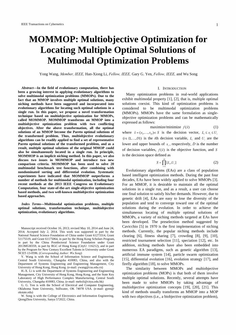
Indeed, Theorem 3 and Theorem 4 reflect the relationship between the original MMOP and the transformed biobjective optimization problem. We give an example to explain the above relationship. For instance, the equal maxima function [25] includes five optimal solutions as shown in Fig. 1(a). After the transformation based on equation (7), these optimal solutions are the Pareto optimal solutions of the transformed biobjective optimization problem, and the objective vectors of them are located on the line segment defined by “y=1-x” (see Fig. 1(b)).

B. Why does MOMMOP Work? After the above introduction of MOMMOP, one may be

interested in the reason why MOMMOP could be effective for MMOPs. We now employ an example to illustrate the principles of MOMMOP.

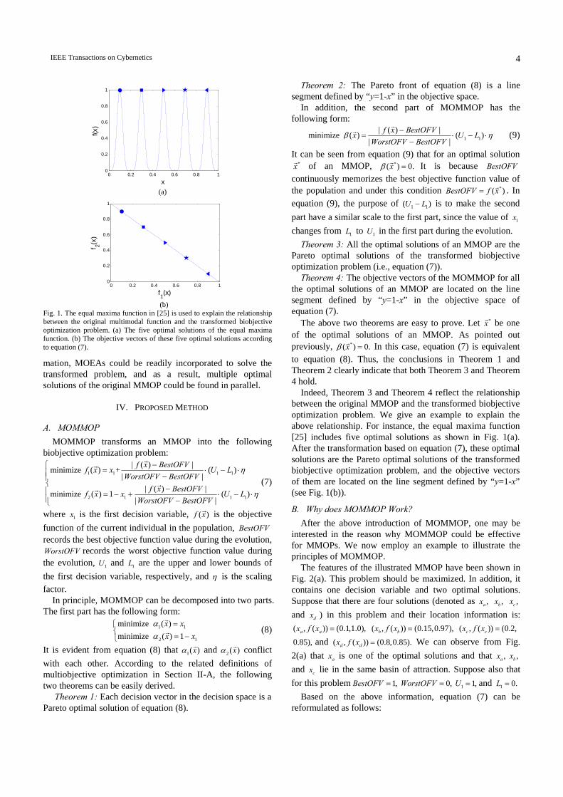
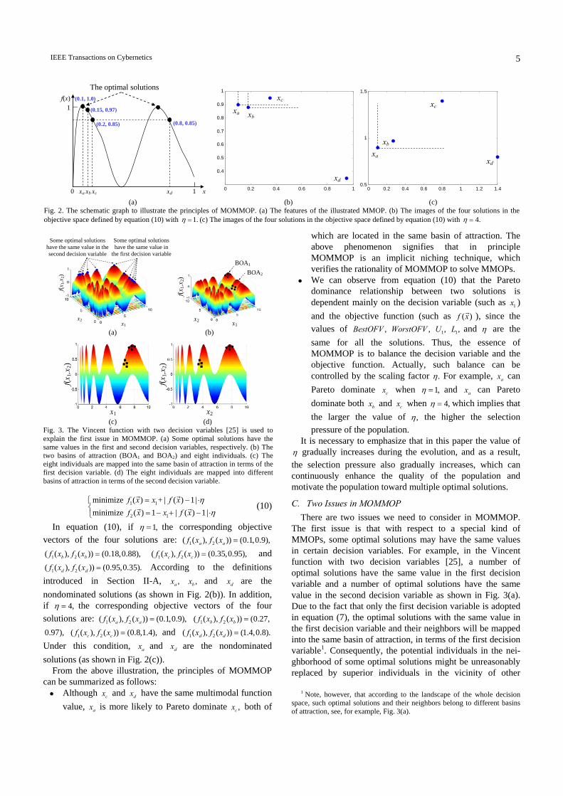
The features of the illustrated MMOP have been shown in Fig. 2(a). This problem should be maximized. In addition, it contains one decision variable and two optimal solutions. Suppose that there are four solutions (denoted as ,ax ,bx ,cx and dx ) in this problem and their location information is: ( , ( )) (0.1,1.0),a ax f x = ( , ( )) (0.15,0.97),b bx f x = ( , ( )) (0.2,c cx f x = 0.85), and ( , ( )) (0.8,0.85).d dx f x = We can observe from Fig. 2(a) that ax is one of the optimal solutions and that ,ax ,bx and cx lie in the same basin of attraction. Suppose also that for this problem 1,BestOFV = 0,WorstOFV = 1 1,U = and 1 0.L =

Based on the above information, equation (7) can be reformulated as follows:

 

0 0.2 0.4 0.6 0.8 10

0.2

0.4

0.6

0.8

1

x

f(x)

(a)

0 0.2 0.4 0.6 0.8 10

0.2

0.4

0.6

0.8

1

f1(x)

f 2(x)

(b) Fig. 1. The equal maxima function in [25] is used to explain the relationship between the original multimodal function and the transformed biobjective optimization problem. (a) The five optimal solutions of the equal maxima function. (b) The objective vectors of these five optimal solutions according to equation (7).

IEEE Transactions on Cybernetics 5

1 1

2 1

minimize ( ) + | ( ) 1|minimize ( ) 1 | ( ) 1|

f x x f xf x x f x

ηη

= − ⋅⎧⎨ = − + − ⋅⎩

(10)

In equation (10), if 1,η = the corresponding objective vectors of the four solutions are: 1 2( ( ), ( )) (0.1,0.9),a af x f x =

1 2( ( ), ( )) (0.18,0.88),b bf x f x = 1 2( ( ), ( )) (0.35,0.95),c cf x f x = and

1 2( ( ), ( )) (0.95,0.35).d df x f x = According to the definitions introduced in Section II-A, ,ax ,bx and dx are the nondominated solutions (as shown in Fig. 2(b)). In addition, if 4,η = the corresponding objective vectors of the four solutions are: 1 2( ( ), ( )) (0.1,0.9),a af x f x = 1 2( ( ), ( )) (0.27,b bf x f x = 0.97), 1 2( ( ), ( )) (0.8,1.4),c cf x f x = and 1 2( ( ), ( )) (1.4,0.8).d df x f x = Under this condition, ax and dx are the nondominated solutions (as shown in Fig. 2(c)).

From the above illustration, the principles of MOMMOP can be summarized as follows:

Although cx and dx have the same multimodal function value, ax is more likely to Pareto dominate ,cx both of

which are located in the same basin of attraction. The above phenomenon signifies that in principle MOMMOP is an implicit niching technique, which verifies the rationality of MOMMOP to solve MMOPs.

We can observe from equation (10) that the Pareto dominance relationship between two solutions is dependent mainly on the decision variable (such as 1x ) and the objective function (such as ( )f x ), since the values of ,BestOFV ,WorstOFV 1,U 1,L and η are the same for all the solutions. Thus, the essence of MOMMOP is to balance the decision variable and the objective function. Actually, such balance can be controlled by the scaling factor .η For example, ax can Pareto dominate cx when 1,η = and ax can Pareto dominate both bx and cx when 4,η = which implies that the larger the value of ,η the higher the selection pressure of the population.

It is necessary to emphasize that in this paper the value of η gradually increases during the evolution, and as a result, the selection pressure also gradually increases, which can continuously enhance the quality of the population and motivate the population toward multiple optimal solutions.

C. Two Issues in MOMMOP There are two issues we need to consider in MOMMOP.

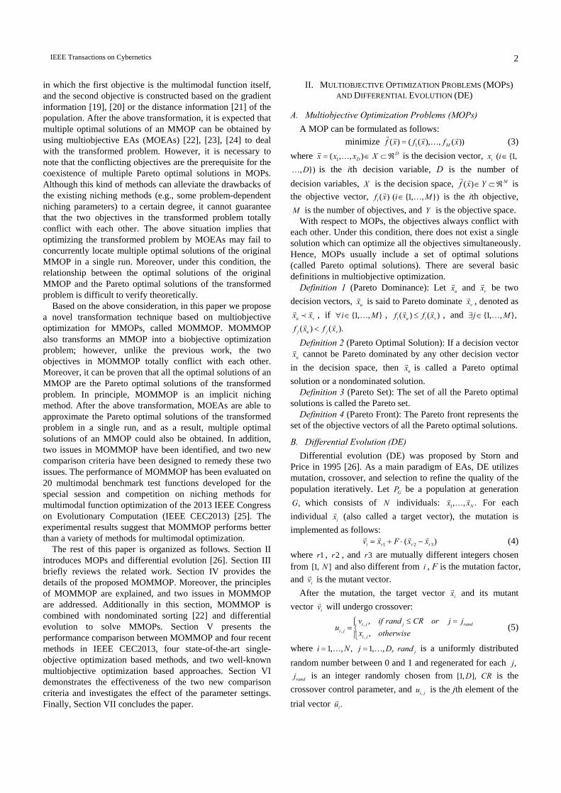
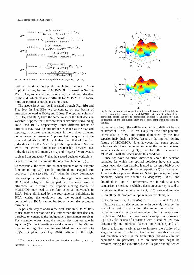
The first issue is that with respect to a special kind of MMOPs, some optimal solutions may have the same values in certain decision variables. For example, in the Vincent function with two decision variables [25], a number of optimal solutions have the same value in the first decision variable and a number of optimal solutions have the same value in the second decision variable as shown in Fig. 3(a). Due to the fact that only the first decision variable is adopted in equation (7), the optimal solutions with the same value in the first decision variable and their neighbors will be mapped into the same basin of attraction, in terms of the first decision variable1. Consequently, the potential individuals in the nei-ghborhood of some optimal solutions might be unreasonably replaced by superior individuals in the vicinity of other

1 Note, however, that according to the landscape of the whole decision space, such optimal solutions and their neighbors belong to different basins of attraction, see, for example, Fig. 3(a).

Some optimal solutions have the same value in the second decision variable

Some optimal solutions have the same value in

the first decision variable

x1 x2

f(x1,x

2)

BOA1

BOA2

f(x1,x

2)

x1x2

(a) (b)

 

f(x1,x

2)

x1

 

x2

f(x1,x

2)

(c) (d)

Fig. 3. The Vincent function with two decision variables [25] is used toexplain the first issue in MOMMOP. (a) Some optimal solutions have the same values in the first and second decision variables, respectively. (b) The two basins of attraction (BOA1 and BOA2) and eight individuals. (c) The eight individuals are mapped into the same basin of attraction in terms of the first decision variable. (d) The eight individuals are mapped into different basins of attraction in terms of the second decision variable.

(0.15, 0.97)

(0.2, 0.85)

0 xa xb xc xd 1 x

(0.1, 1.0)

(0.8, 0.85)

f(x)

1

The optimal solutions

0 0.2 0.4 0.6 0.8 1

0.4

0.5

0.6

0.7

0.8

0.9

1

xa xb

xc

xd

0 0.2 0.4 0.6 0.8 1 1.2 1.40.5

1

1.5

xa

xb

xc

xd

(a) (b) (c)

Fig. 2. The schematic graph to illustrate the principles of MOMMOP. (a) The features of the illustrated MMOP. (b) The images of the four solutions in the objective space defined by equation (10) with 1.η = (c) The images of the four solutions in the objective space defined by equation (10) with 4.η =

IEEE Transactions on Cybernetics 6

optimal solutions during the evolution, because of the implicit niching feature of MOMMOP discussed in Section IV-B. Thus, some potential regions may include no individual in the end, which makes it difficult for MOMMOP to locate multiple optimal solutions in a single run.

The above issue can be illustrated through Fig. 3(b) and Fig. 3(c). In Fig. 3(b), we concentrate on two basins of attraction denoted as BOA1 and BOA2. The optimal solutions in BOA1 and BOA2 have the same value in the first decision variable. Suppose that there are four individuals surrounding BOA1 and BOA2, respectively. Since different basins of attraction may have distinct properties (such as the size and topology structure), the individuals in them show different convergence performance. Suppose that the quality of the four individuals in BOA1 is higher than that of the four individuals in BOA2. According to the explanation in Section IV-B, the Pareto dominance relationship between two individuals depends mainly on 1x and 1 2( , ).f x x 2 Moreover, it is clear from equation (7) that the second decision variable 2x is only exploited to compute the objective function 1 2( , ).f x x Consequently, the three-dimensional structure of the Vincent function in Fig. 3(a) can be simplified and mapped into

1 1 2O ( , )x f x x plane (see Fig. 3(c)) when the Pareto dominance relationship is considered. Thus, the eight individuals in BOA1 and BOA2 will be mapped into the same basin of attraction. As a result, the implicit niching feature of MOMMOP may lead to the four potential individuals in BOA2 being eliminated by the four superior individuals in BOA1 during the evolution, and the optimal solution contained by BOA2 cannot be found when the evolution terminates.

A possible way to address the first issue in MOMMOP is to use another decision variable, rather than the first decision variable, to construct the biobjective optimization problem. For example, when using the second decision variable in equation (7), the three-dimensional structure of the Vincent function in Fig. 3(a) can be simplified and mapped into

2 1 2O ( , )x f x x plane (see Fig. 3(d)). Afterward, the eight

2 The Vincent function involves two decision variable 1x and 2 ,x

therefore 1 2( ) ( , ).f x f x x=

individuals in Fig. 3(b) will be mapped into different basins of attraction. Thus, it is less likely that the four potential individuals in BOA2 are Pareto dominated by the four superior individuals in BOA1 based on the implicit niching feature of MOMMOP. Note, however, that some optimal solutions also have the same value in the second decision variable as shown in Fig. 3(a); therefore, the first issue in MOMMOP will still occur under this condition.

Since we have no prior knowledge about the decision variables for which the optimal solutions have the same values, each decision variable is used to design a biobjective optimization problem similar to equation (7) in this paper. After the above process, there are D biobjective optimization problems, which are denoted as 1 2, , , DBOP BOP BOP… and described in Fig. 4. Furthermore, we introduce a new comparison criterion, in which a decision vector ux is said to dominate another decision vector vx if ux Pareto dominates

vx on all the D biobjective optimization problems, i.e.,

1 2 on on on u v u v u v Dx x BOP x x BOP x x BOP∧ ∧ ∧≺ ≺ ≺ (11) Next, we explain the second issue. In general, the larger the

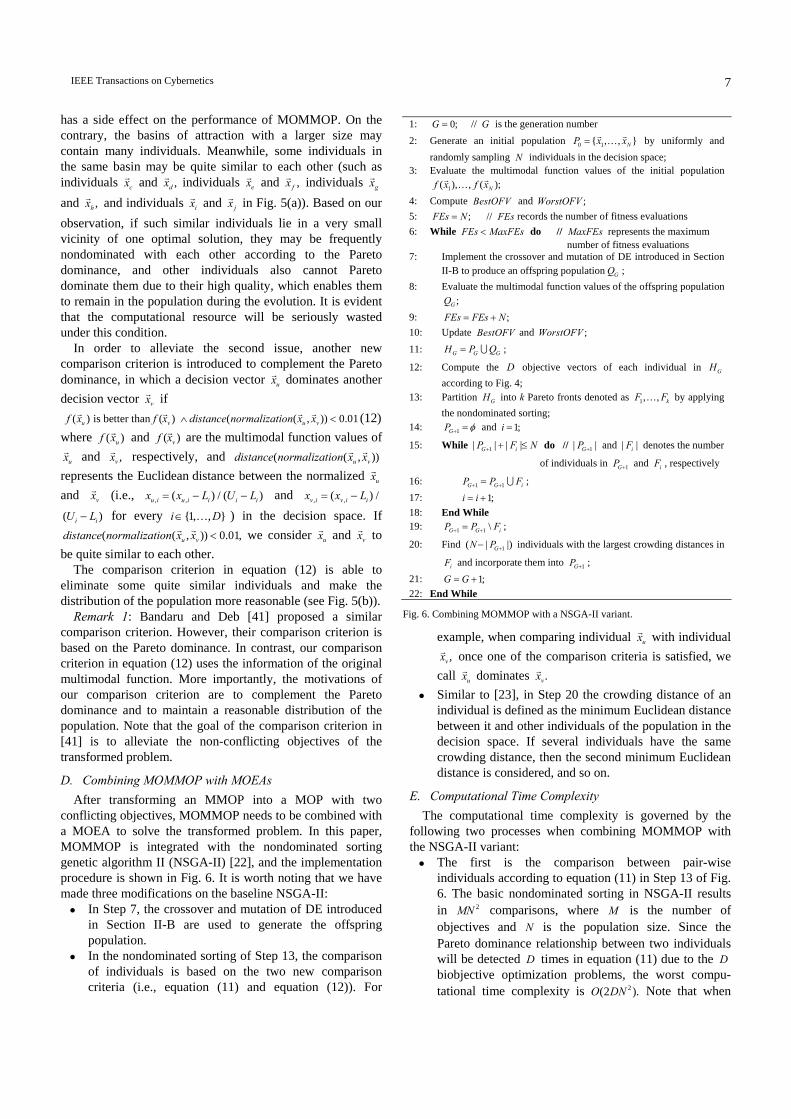
size of a basin of attraction, the more the number of individuals located in it, and vice versa. The first composition function in [25] has been taken as an example. As shown in Fig. 5(a), the basins of attraction with a smaller size may contain only one individual (such as individuals ax and bx ). Note that it is not a trivial task to improve the quality of a single individual in a basin of attraction through crossover and mutation since it is far from other individuals in the population. In particular, such an individual might be removed during the evolution due to its poor quality, which

1 1 1

1

1 1 1

2 2 2

2

2

| ( ) |minimize + ( )| |

| ( ) |minimize 1 ( )| || ( ) |minimize + ( )

| |

minimize 1

f x BestOFVx U LWorstOFV BestOFV

BOPf x BestOFVx U L

WorstOFV BestOFVf x BestOFVx U L

WorstOFV BestOFVBOP

x

η

η

η

−⎧ ⋅ − ⋅⎪ −⎪⎨ −⎪ − + ⋅ − ⋅⎪ −⎩

−⋅ − ⋅

−

− + 2 2| ( ) | ( )

| |

| ( ) |minimize + ( )| |

| ( ) |minimize 1|

D D D

D

D

f x BestOFV U LWorstOFV BestOFV

f x BestOFVx U LWorstOFV BestOFV

BOPf x BestOFVx

WorstOFV

η

η

⎧⎪⎪⎨ −⎪ ⋅ − ⋅⎪ −⎩

−⋅ − ⋅

−−

− + ( )| D DU L

BestOFVη

⎧⎪⎪⎨⎪ ⋅ − ⋅⎪ −⎩

Fig. 4. D biobjective optimization problems 1 2, , , .DBOP BOP BOP…

ax

bx  

cx dx

gx  

hx

ix jx

ex fx

f(x1,x

2)

x1 x2

(a)

f(x1,x

2)

x1 x2

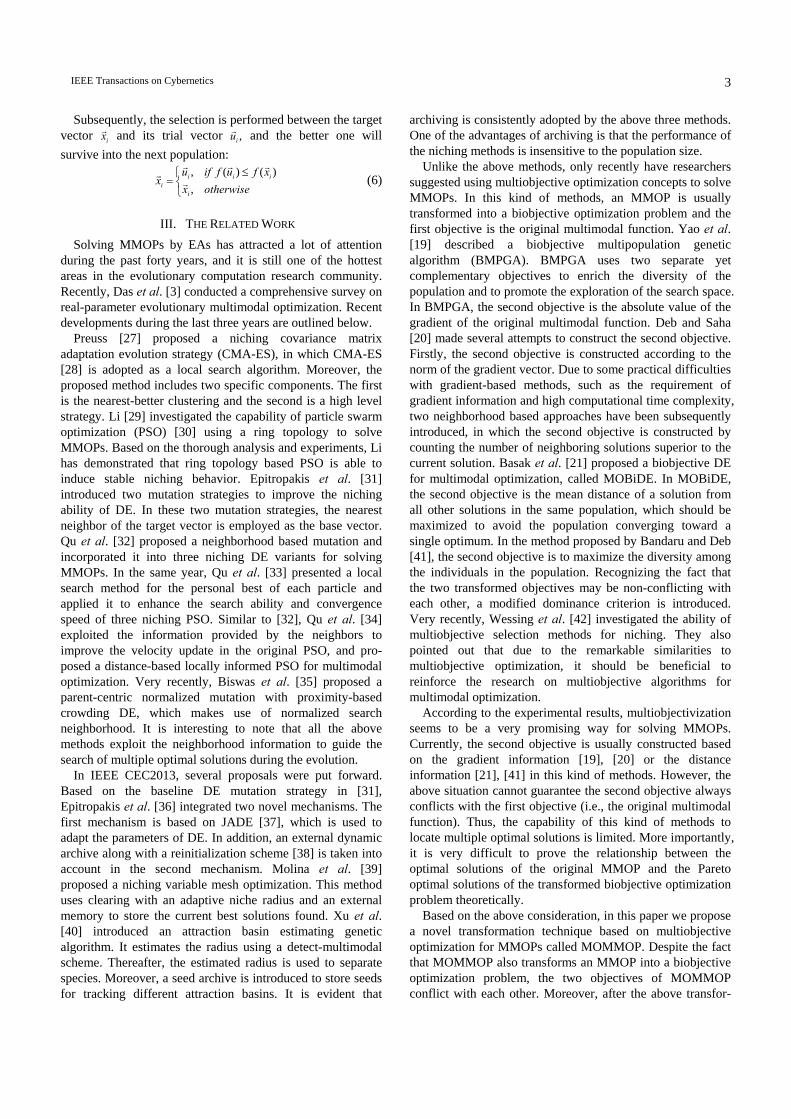
(b) Fig. 5. The first composition function with two decision variables in [25] is used to explain the second issue in MOMMOP. (a) The distribution of the population before the second comparison criterion is utilized. (b) The distribution of the population after the second comparison criterion is utilized.

IEEE Transactions on Cybernetics 7

has a side effect on the performance of MOMMOP. On the contrary, the basins of attraction with a larger size may contain many individuals. Meanwhile, some individuals in the same basin may be quite similar to each other (such as individuals cx and ,dx individuals ex and ,fx individuals gx and ,hx and individuals ix and jx in Fig. 5(a)). Based on our observation, if such similar individuals lie in a very small vicinity of one optimal solution, they may be frequently nondominated with each other according to the Pareto dominance, and other individuals also cannot Pareto dominate them due to their high quality, which enables them to remain in the population during the evolution. It is evident that the computational resource will be seriously wasted under this condition.

In order to alleviate the second issue, another new comparison criterion is introduced to complement the Pareto dominance, in which a decision vector ux dominates another decision vector vx if

( ) is better than ( ) ( ( , )) 0.01u v u vf x f x distance normalization x x∧ < (12) where ( )uf x and ( )vf x are the multimodal function values of

ux and ,vx respectively, and ( ( , ))u vdistance normalization x x represents the Euclidean distance between the normalized ux and vx (i.e., , ,( ) / ( )u i u i i i ix x L U L= − − and , ,( ) /v i v i ix x L= − ( )i iU L− for every {1, , }i D∈ … ) in the decision space. If

( ( , )) 0.01,u vdistance normalization x x < we consider ux and vx to be quite similar to each other.

The comparison criterion in equation (12) is able to eliminate some quite similar individuals and make the distribution of the population more reasonable (see Fig. 5(b)).

Remark 1: Bandaru and Deb [41] proposed a similar comparison criterion. However, their comparison criterion is based on the Pareto dominance. In contrast, our comparison criterion in equation (12) uses the information of the original multimodal function. More importantly, the motivations of our comparison criterion are to complement the Pareto dominance and to maintain a reasonable distribution of the population. Note that the goal of the comparison criterion in [41] is to alleviate the non-conflicting objectives of the transformed problem.

D. Combining MOMMOP with MOEAs After transforming an MMOP into a MOP with two

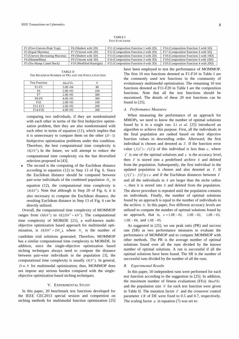
conflicting objectives, MOMMOP needs to be combined with a MOEA to solve the transformed problem. In this paper, MOMMOP is integrated with the nondominated sorting genetic algorithm II (NSGA-II) [22], and the implementation procedure is shown in Fig. 6. It is worth noting that we have made three modifications on the baseline NSGA-II:

In Step 7, the crossover and mutation of DE introduced in Section II-B are used to generate the offspring population.

In the nondominated sorting of Step 13, the comparison of individuals is based on the two new comparison criteria (i.e., equation (11) and equation (12)). For

example, when comparing individual ux with individual ,vx once one of the comparison criteria is satisfied, we

call ux dominates .vx Similar to [23], in Step 20 the crowding distance of an

individual is defined as the minimum Euclidean distance between it and other individuals of the population in the decision space. If several individuals have the same crowding distance, then the second minimum Euclidean distance is considered, and so on.

E. Computational Time Complexity The computational time complexity is governed by the

following two processes when combining MOMMOP with the NSGA-II variant:

The first is the comparison between pair-wise individuals according to equation (11) in Step 13 of Fig. 6. The basic nondominated sorting in NSGA-II results in 2MN comparisons, where M is the number of objectives and N is the population size. Since the Pareto dominance relationship between two individuals will be detected D times in equation (11) due to the D biobjective optimization problems, the worst compu-tational time complexity is 2(2 ).O DN Note that when

1: 0;G = // G is the generation number 2: Generate an initial population 0 1{ , , }NP x x= … by uniformly and

randomly sampling N individuals in the decision space; 3: Evaluate the multimodal function values of the initial population

1( ), , ( );Nf x f x… 4: Compute BestOFV and ;WorstOFV 5: ;FEs N= // FEs records the number of fitness evaluations 6: While FEs MaxFEs< do // MaxFEs represents the maximum

number of fitness evaluations 7: Implement the crossover and mutation of DE introduced in Section

II-B to produce an offspring population GQ ; 8: Evaluate the multimodal function values of the offspring population

;GQ 9: ;FEs FEs N= + 10: Update BestOFV and ;WorstOFV 11: G G GH P Q= ∪ ;

12: Compute the D objective vectors of each individual in GH according to Fig. 4;

13: Partition GH into k Pareto fronts denoted as 1, , kF F… by applying the nondominated sorting;

14: 1GP φ+ = and 1;i =

15: While 1| | | |G iP F N+ + ≤ do // 1| |GP + and | |iF denotes the number

of individuals in 1GP + and iF , respectively

16: 1 1G G iP P F+ += ∪ ; 17: 1;i i= + 18: End While 19: 1 1 \G G iP P F+ += ;

20: Find 1( | |)GN P +− individuals with the largest crowding distances in

iF and incorporate them into 1GP + ; 21: 1;G G= + 22: End While

Fig. 6. Combining MOMMOP with a NSGA-II variant.

IEEE Transactions on Cybernetics 8

comparing two individuals, if they are nondominated with each other in terms of the first biobjective optimi-zation problem, then they are also nondominated with each other in terms of equation (11), which implies that it is unnecessary to compare them on the other ( 1)D − biobjective optimization problems under this condition. Therefore, the best computational time complexity is

2(2 ).O N In the future, we will attempt to reduce the computational time complexity via the fast diversified selection proposed in [43].

The second is the computing of the Euclidean distance according to equation (12) in Step 13 of Fig. 6. Since the Euclidean distance should be computed between pair-wise individuals of the combined population GH in equation (12), the computational time complexity is

2(4 ).O N Note that although in Step 20 of Fig. 6, it is also necessary to compute the Euclidean distance, the resulting Euclidean distance in Step 13 of Fig. 6 can be directly utilized.

Overall, the computational time complexity of MOMMOP ranges from 2(6 )O N to 2 2(2 4 ).O DN N+ The computational time complexity of MOBiDE [21], a well-known multi-objective optimization based approach for multimodal opti-mization, is 2( ),gO DN DN+ where gN is the number of candidate trial solutions generated. Therefore, MOMMOP has a similar computational time complexity to MOBiDE. In addition, since the single-objective optimization based niching techniques always need to compute the distance between pair-wise individuals in the population [3], the computational time complexity is usually 2( ).O N In general, D N for multimodal optimization; thus, MOMMOP does not impose any serious burden compared with the single-objective optimization based niching techniques.

V. EXPERIMENTAL STUDY In this paper, 20 benchmark test functions developed for

the IEEE CEC2013 special session and competition on niching methods for multimodal function optimization [25]

have been employed to test the performance of MOMMOP. The first 10 test functions denoted as F1-F10 in Table I are the commonly used test functions in the community of evolutionary multimodal optimization. The remaining 10 test functions denoted as F11-F20 in Table I are the composition functions. Note that all the test functions should be maximized. The details of these 20 test functions can be found in [25].

A. Performance Measures When measuring the performance of an approach for

MMOPs, we need to know the number of optimal solutions found by it in a single run. Li et al. [25] introduced an algorithm to achieve this purpose. First, all the individuals in the final population are ranked based on their objective function values in descending order. Afterward, the first individual is chosen and denoted as .x′ If the function error value *( ( ) ( ))f x f x′− of this individual is less than ,ε where

*x is one of the optimal solutions and ε is the accuracy level, then x′ is stored into a predefined archive S and deleted from the population. Subsequently, the first individual in the updated population is chosen and also denoted as .x′ If

*( ( ) ( ))f x f x ε′− ≤ and if the Euclidean distances between x′ and all the individuals in S are larger than the niche radius

,r then it is stored into S and deleted from the population. The above procedure is repeated until the population contains no individuals. Finally, the number of optimal solutions found by an approach is equal to the number of individuals in the archive .S In this paper, five different accuracy levels are utilized to compute the number of optimal solutions found by an approach, that is, 1.0E 01,ε = − 1.0E 02,− 1.0E 03,− 1.0E 04,− and 1.0E 05.−

As suggested in [25], we use peak ratio (PR) and success rate (SR) as two performance measures to evaluate the performance of MOMMOP and to compare MOMMOP with other methods. The PR is the average number of optimal solutions found over all the runs divided by the known number of optimal solutions. A run is successful if all the optimal solutions have been found. The SR is the number of successful runs divided by the number of all the runs.

B. Experimental Results In this paper, 50 independent runs were performed for each

test function according to the suggestion in [25]. In addition, the maximum number of fitness evaluations (FEs) MaxFEs and the population size N for each test function were given in Table II. The mutation factor F and the crossover control parameter CR of DE were fixed to 0.5 and 0.7, respectively. The scaling factor η in equation (7) was set to:

TABLE I TEST FUNCTIONS

F1 (Five-Uneven-Peak Trap) F6 (Shubert with 2D) F11 (Composition Function 1 with 2D) F16 (Composition Function 3 with 5D) F2 (Equal Maxima) F7 (Vincent with 2D) F12 (Composition Function 2 with 2D) F17 (Composition Function 4 with 5D) F3 (Uneven Decreasing Maxima) F8 (Shubert with 3D) F13 (Composition Function 3 with 2D) F18 (Composition Function 3 with 10D) F4 (Himmelblau) F9 (Vincent with 3D) F14 (Composition Function 3 with 3D) F19 (Composition Function 4 with 10D) F5 (Six-Hump Camel Back) F10 (Modified Rastrigin) F15 (Composition Function 4 with 3D) F20 (Composition Function 4 with 20D)

TABLE II THE MAXIMUM NUMBER OF FES AND THE POPULATION SIZE

Test Function MaxFEs N

F1-F5 5.0E+04 80 F6 2.0E+05 100 F7 2.0E+05 300

F8-F9 4.0E+05 300 F10 2.0E+05 100

F11-F13 2.0E+05 200 F14-F20 4.0E+05 200

IEEE Transactions on Cybernetics 9

340 ( )D CurrentFEs MaxFEsη = (13) where CurrentFEs represents the current number of FEs.

The PR and SR values provided by MOMMOP at five different accuracy levels for 20 test functions are summarized in the supplemental file. MOMMOP achieves 100% PR and 100% SR for the first 10 test functions at all the accuracy levels except for test function F9, which means that MOMMOP has the capability to solve these test functions consistently. F9 involves 216 optimal solutions and the distances among these optimal solutions vary remarkably. Therefore, it is a very challenging task for the current methods to maintain all the optimal solutions of F9 in a single run. Note that for F9, 100% PR and 100% SR have been accomplished by MOMMOP at the first three accuracy levels (i.e., 1.0E 01,ε = − 1.0E 02,− and 1.0E 03).− Moreover, the PR values surpass 0.97 for the other two accuracy levels, which implies that all the individuals in the population lie in a very small vicinity of diverse optimal solutions. The 10 compo-sition functions are more complex than others. With respect to these composition functions, MOMMOP consistently converges to multiple optimal solutions except that only one optimal solution has been found for F20. We can also observe from the supplemental file that the successful runs arise for F11-F13. In particular, MOMMOP is able to consistently locate all the optimal solutions of F11 at the first accuracy level (i.e., 1.0E 01).ε = −

The supplemental file plots the evolution of the average number of optimal solutions found by MOMMOP over 50 runs against the number of FEs for 20 test functions with 1.0E 04.ε = − The supplemental file clearly indicates that MOMMOP can not only find multiple optimal solutions for all the test functions with the exception of F20, but can also maintain these optimal solutions found during the evolution.

C. Comparison with Four Recent Methods in IEEE CEC2013

Four methods have participated the special session and competition on niching methods for multimodal function optimization organized by Li et al. [25] in IEEE CEC2013. They are dADE/nrand/1 [36], NVMO [39], PNSGA-II [41], and modified NSGA-II [20] (called MNSGA-II in this paper), which have been briefly introduced in Section III. The performance of MOMMOP was first compared with that of these four recent methods. The experimental results of these four methods were directly taken from the original papers in order to ensure a fair comparison. It is worth noting that all the five compared methods implemented 50 independent runs and used the same MaxFEs for each test function.

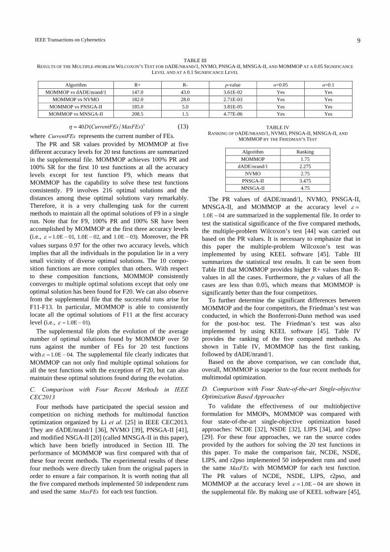
The PR values of dADE/nrand/1, NVMO, PNSGA-II, MNSGA-II, and MOMMOP at the accuracy level ε = 1.0E 04− are summarized in the supplemental file. In order to test the statistical significance of the five compared methods, the multiple-problem Wilcoxon’s test [44] was carried out based on the PR values. It is necessary to emphasize that in this paper the multiple-problem Wilcoxon’s test was implemented by using KEEL software [45]. Table III summarizes the statistical test results. It can be seen from Table III that MOMMOP provides higher R+ values than R- values in all the cases. Furthermore, the p values of all the cases are less than 0.05, which means that MOMMOP is significantly better than the four competitors.

To further determine the significant differences between MOMMOP and the four competitors, the Friedman’s test was conducted, in which the Bonferroni-Dunn method was used for the post-hoc test. The Friedman’s test was also implemented by using KEEL software [45]. Table IV provides the ranking of the five compared methods. As shown in Table IV, MOMMOP has the first ranking, followed by dADE/nrand/1.

Based on the above comparison, we can conclude that, overall, MOMMOP is superior to the four recent methods for multimodal optimization.

D. Comparison with Four State-of-the-art Single-objective Optimization Based Approaches

To validate the effectiveness of our multiobjective formulation for MMOPs, MOMMOP was compared with four state-of-the-art single-objective optimization based approaches: NCDE [32], NSDE [32], LIPS [34], and r2pso [29]. For these four approaches, we ran the source codes provided by the authors for solving the 20 test functions in this paper. To make the comparison fair, NCDE, NSDE, LIPS, and r2pso implemented 50 independent runs and used the same MaxFEs with MOMMOP for each test function. The PR values of NCDE, NSDE, LIPS, r2pso, and MOMMOP at the accuracy level 1.0E 04ε = − are shown in the supplemental file. By making use of KEEL software [45],

TABLE III RESULTS OF THE MULTIPLE-PROBLEM WILCOXON’S TEST FOR DADE/NRAND/1, NVMO, PNSGA-II, MNSGA-II, AND MOMMOP AT A 0.05 SIGNIFICANCE

LEVEL AND AT A 0.1 SIGNIFICANCE LEVEL

Algorithm R+ R- p-value α=0.05 α=0.1 MOMMOP vs dADE/nrand/1 147.0 43.0 3.61E-02 Yes Yes

MOMMOP vs NVMO 182.0 28.0 2.71E-03 Yes Yes MOMMOP vs PNSGA-II 185.0 5.0 3.81E-05 Yes Yes MOMMOP vs MNSGA-II 208.5 1.5 4.77E-06 Yes Yes

TABLE IV RANKING OF DADE/NRAND/1, NVMO, PNSGA-II, MNSGA-II, AND

MOMMOP BY THE FRIEDMAN’S TEST

Algorithm Ranking MOMMOP 1.75

dADE/nrand/1 2.275 NVMO 2.75

PNSGA-II 3.475 MNSGA-II 4.75

IEEE Transactions on Cybernetics 10

the multiple-problem Wilcoxon’s test and the Friedman’s test have been implemented based on the PR values. Tables V and VI present the experimental results.

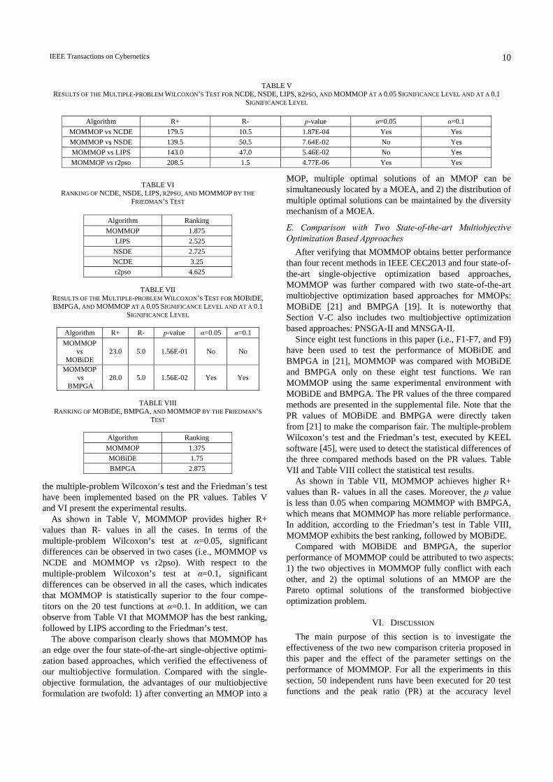
As shown in Table V, MOMMOP provides higher R+ values than R- values in all the cases. In terms of the multiple-problem Wilcoxon’s test at α=0.05, significant differences can be observed in two cases (i.e., MOMMOP vs NCDE and MOMMOP vs r2pso). With respect to the multiple-problem Wilcoxon’s test at α=0.1, significant differences can be observed in all the cases, which indicates that MOMMOP is statistically superior to the four compe-titors on the 20 test functions at α=0.1. In addition, we can observe from Table VI that MOMMOP has the best ranking, followed by LIPS according to the Friedman’s test.

The above comparison clearly shows that MOMMOP has an edge over the four state-of-the-art single-objective optimi-zation based approaches, which verified the effectiveness of our multiobjective formulation. Compared with the single-objective formulation, the advantages of our multiobjective formulation are twofold: 1) after converting an MMOP into a

MOP, multiple optimal solutions of an MMOP can be simultaneously located by a MOEA, and 2) the distribution of multiple optimal solutions can be maintained by the diversity mechanism of a MOEA.

E. Comparison with Two State-of-the-art Multiobjective Optimization Based Approaches

After verifying that MOMMOP obtains better performance than four recent methods in IEEE CEC2013 and four state-of-the-art single-objective optimization based approaches, MOMMOP was further compared with two state-of-the-art multiobjective optimization based approaches for MMOPs: MOBiDE [21] and BMPGA [19]. It is noteworthy that Section V-C also includes two multiobjective optimization based approaches: PNSGA-II and MNSGA-II.

Since eight test functions in this paper (i.e., F1-F7, and F9) have been used to test the performance of MOBiDE and BMPGA in [21], MOMMOP was compared with MOBiDE and BMPGA only on these eight test functions. We ran MOMMOP using the same experimental environment with MOBiDE and BMPGA. The PR values of the three compared methods are presented in the supplemental file. Note that the PR values of MOBiDE and BMPGA were directly taken from [21] to make the comparison fair. The multiple-problem Wilcoxon’s test and the Friedman’s test, executed by KEEL software [45], were used to detect the statistical differences of the three compared methods based on the PR values. Table VII and Table VIII collect the statistical test results.

As shown in Table VII, MOMMOP achieves higher R+ values than R- values in all the cases. Moreover, the p value is less than 0.05 when comparing MOMMOP with BMPGA, which means that MOMMOP has more reliable performance. In addition, according to the Friedman’s test in Table VIII, MOMMOP exhibits the best ranking, followed by MOBiDE.

Compared with MOBiDE and BMPGA, the superior performance of MOMMOP could be attributed to two aspects: 1) the two objectives in MOMMOP fully conflict with each other, and 2) the optimal solutions of an MMOP are the Pareto optimal solutions of the transformed biobjective optimization problem.

VI. DISCUSSION The main purpose of this section is to investigate the

effectiveness of the two new comparison criteria proposed in this paper and the effect of the parameter settings on the performance of MOMMOP. For all the experiments in this section, 50 independent runs have been executed for 20 test functions and the peak ratio (PR) at the accuracy level

TABLE VI RANKING OF NCDE, NSDE, LIPS, R2PSO, AND MOMMOP BY THE

FRIEDMAN’S TEST

Algorithm Ranking MOMMOP 1.875

LIPS 2.525 NSDE 2.725 NCDE 3.25 r2pso 4.625

TABLE VII

RESULTS OF THE MULTIPLE-PROBLEM WILCOXON’S TEST FOR MOBIDE, BMPGA, AND MOMMOP AT A 0.05 SIGNIFICANCE LEVEL AND AT A 0.1

SIGNIFICANCE LEVEL

Algorithm R+ R- p-value α=0.05 α=0.1 MOMMOP

vs MOBiDE

23.0 5.0 1.56E-01 No No

MOMMOP vs

BMPGA 28.0 5.0 1.56E-02 Yes Yes

TABLE VIII

RANKING OF MOBIDE, BMPGA, AND MOMMOP BY THE FRIEDMAN’S TEST

Algorithm Ranking MOMMOP 1.375 MOBiDE 1.75 BMPGA 2.875

TABLE V RESULTS OF THE MULTIPLE-PROBLEM WILCOXON’S TEST FOR NCDE, NSDE, LIPS, R2PSO, AND MOMMOP AT A 0.05 SIGNIFICANCE LEVEL AND AT A 0.1

SIGNIFICANCE LEVEL

Algorithm R+ R- p-value α=0.05 α=0.1 MOMMOP vs NCDE 179.5 10.5 1.87E-04 Yes Yes MOMMOP vs NSDE 139.5 50.5 7.64E-02 No Yes MOMMOP vs LIPS 143.0 47.0 5.46E-02 No Yes MOMMOP vs r2pso 208.5 1.5 4.77E-06 Yes Yes

IEEE Transactions on Cybernetics 11

1.0E 04ε = − has been recorded. Moreover, in order to show the significant differences of the compared methods, the multiple-problem Wilcoxon’s test and the Friedman’s test have been conducted by making use of KEEL software [45] based on the PR values. The parameter settings were kept unchanged unless we point out that new settings for one or some of the parameters have been adopted with the aim of parameter study.

A. Effectiveness of Two New Comparison Criteria In Section IV-C, we discuss two issues in MOMMOP and

introduce two new comparison criteria (i.e., equations (11) and (12)). In order to ascertain the effectiveness of these two comparison criteria, two additional experiments have been carried out. In this first experiment, only one biobjective optimization problem rather than D biobjective optimization problems is constructed, by taking advantage of one randomly chosen decision variable ( {1, , })ix i D∈ … at each generation. This MOMMOP variant is called MOMMOP1. The second experiment removes the second comparison criterion and is denoted as MOMMOP2. The PR values of MOMMOP1, MOMMOP2, and MOMMOP are summarized in the supplemental file.

1) Effectiveness of the First New Comparison Criterion: The PR values derived from MOMMOP1 drastically decrease for nine test functions (i.e., F7-F9, F11, F12, F15, and F17-F19) compared with those provided by MOMMOP. Among these nine test functions, F7-F9 have a unique characteristic (i.e., some optimal solutions have the same values in certain decision variables). As analyzed in Section IV-C, for this kind of MMOPs, if only one decision variable is chosen to construct the biobjective optimization problem in equation (7), some potential individuals might be eliminated from the population unreasonably and some basins of attraction will be neglected during the evolution. Therefore, MOMMOP1 suffers from significant performance degradation for these three test functions. In F11, F12, F15, and F17-F19, the values of certain decision variables are very similar for some optimal solutions; therefore, MOMMOP1 faces a similar

difficulty as in F7-F9 when solving these six test functions. It is interesting to note that although F6 and F10 belong to the same kind of MMOPs as F7-F9, there is no performance difference between MOMMOP and MOMMOP1 for them. It may be because the individuals in different basins of attraction have similar convergence speed and quality. As a result, the possibility that the replacement takes place over different basins of attraction drastically decreases, and MOMMOP1 can succeed in locating all the optimal solutions at the end of a run.

We can conclude from the above comparison that the first new comparison criterion is quite effective for solving the MMOPs in which some optimal solutions have the same or similar values in certain decision variables.

2) Effectiveness of the Second New Comparison Criterion: The PR values provided by MOMMOP are of a higher quality than those of MOMMOP2 for 13 test functions (i.e., F4, F7-F9, and F11-F19). Moreover, it can be observed that the PR values of MOMMOP2 are less than 0.1 for six test functions (i.e., F4, F14-F16, F18, and F19). Especially, MOMMOP2 cannot find any optimal solution for F18.

The above comparison suggests that MOMMOP2 cannot maintain as many optimal solutions as MOMMOP for a majority of test functions, and that MOMMOP2 is unable to provide the results with high accuracy for some complex test functions. The poor performance of MOMMOP2 can be attributed to its inability to make an appropriate distribution of the population. The above experimental results also demonstrate the effectiveness of the second new comparison criterion to balance the population distribution.

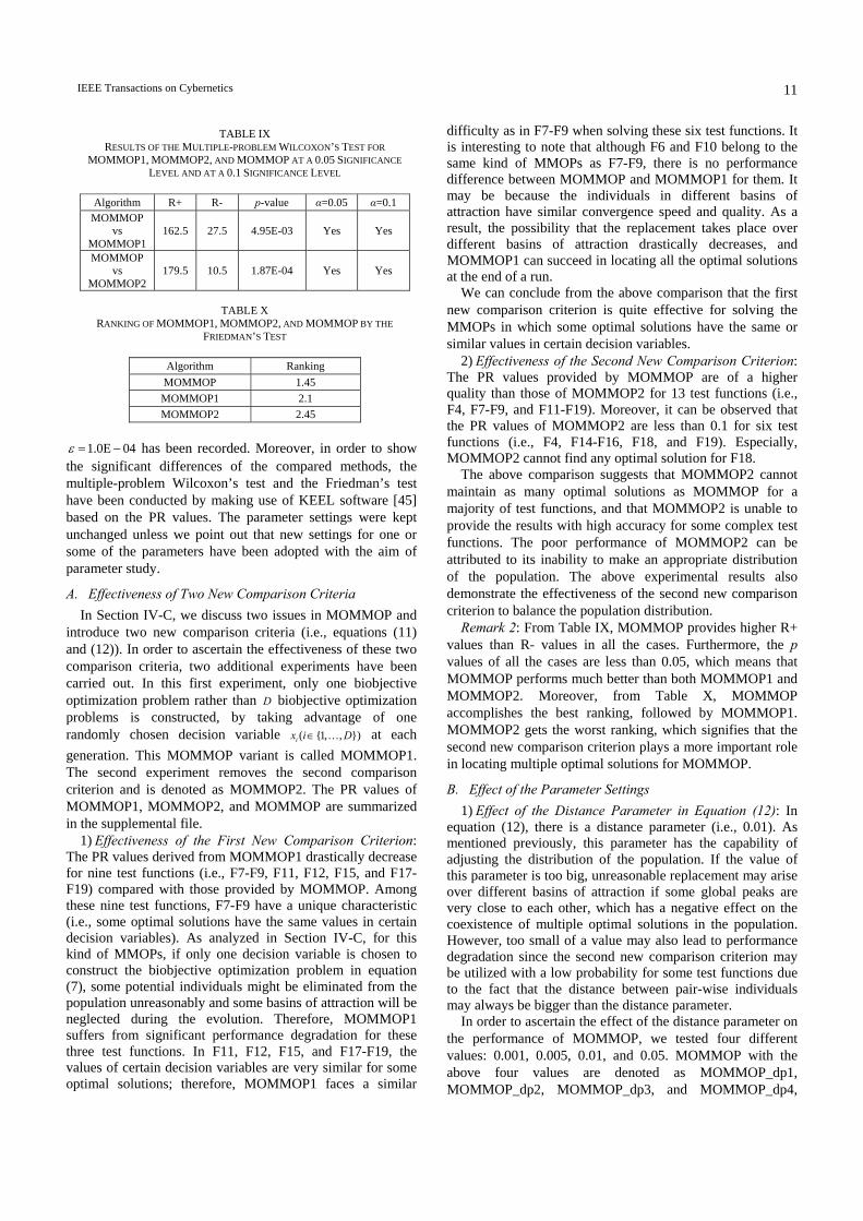
Remark 2: From Table IX, MOMMOP provides higher R+ values than R- values in all the cases. Furthermore, the p values of all the cases are less than 0.05, which means that MOMMOP performs much better than both MOMMOP1 and MOMMOP2. Moreover, from Table X, MOMMOP accomplishes the best ranking, followed by MOMMOP1. MOMMOP2 gets the worst ranking, which signifies that the second new comparison criterion plays a more important role in locating multiple optimal solutions for MOMMOP.

B. Effect of the Parameter Settings 1) Effect of the Distance Parameter in Equation (12): In

equation (12), there is a distance parameter (i.e., 0.01). As mentioned previously, this parameter has the capability of adjusting the distribution of the population. If the value of this parameter is too big, unreasonable replacement may arise over different basins of attraction if some global peaks are very close to each other, which has a negative effect on the coexistence of multiple optimal solutions in the population. However, too small of a value may also lead to performance degradation since the second new comparison criterion may be utilized with a low probability for some test functions due to the fact that the distance between pair-wise individuals may always be bigger than the distance parameter.

In order to ascertain the effect of the distance parameter on the performance of MOMMOP, we tested four different values: 0.001, 0.005, 0.01, and 0.05. MOMMOP with the above four values are denoted as MOMMOP_dp1, MOMMOP_dp2, MOMMOP_dp3, and MOMMOP_dp4,

TABLE IX RESULTS OF THE MULTIPLE-PROBLEM WILCOXON’S TEST FOR

MOMMOP1, MOMMOP2, AND MOMMOP AT A 0.05 SIGNIFICANCE LEVEL AND AT A 0.1 SIGNIFICANCE LEVEL

Algorithm R+ R- p-value α=0.05 α=0.1 MOMMOP

vs MOMMOP1

162.5 27.5 4.95E-03 Yes Yes

MOMMOP vs

MOMMOP2 179.5 10.5 1.87E-04 Yes Yes

TABLE X

RANKING OF MOMMOP1, MOMMOP2, AND MOMMOP BY THE FRIEDMAN’S TEST

Algorithm Ranking MOMMOP 1.45 MOMMOP1 2.1 MOMMOP2 2.45

IEEE Transactions on Cybernetics 12

respectively. The PR values of these four algorithms are summarized in the supplemental file.

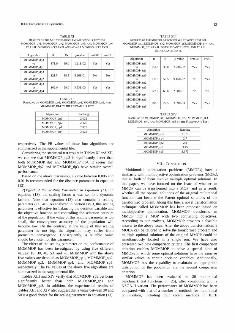
Considering the statistical test results in Tables XI and XII, we can see that MOMMOP_dp3 is significantly better than both MOMMOP_dp1 and MOMMOP_dp4. It seems that MOMMOP_dp2 and MOMMOP_dp3 have similar overall performance.

Based on the above discussion, a value between 0.005 and 0.01 is recommended for the distance parameter in equation (12).

2) Effect of the Scaling Parameter in Equation (13): In equation (13), the scaling factor η was set in a dynamic fashion. Note that equation (13) also contains a scaling parameter (i.e., 40). As analyzed in Section IV-B, this scaling parameter is effective for balancing the decision variable and the objective function and controlling the selection pressure of the population. If the value of this scaling parameter is too small, the convergence accuracy of the population will become low. On the contrary, if the value of this scaling parameter is too big, the algorithm may suffer from premature convergence. Consequently, a suitable value should be chosen for this parameter.

The effect of the scaling parameter on the performance of MOMMOP has been investigated by using five different values: 10, 30, 40, 50, and 70. MOMMOP with the above five values are denoted as MOMMOP_sp1, MOMMOP_sp2, MOMMOP_sp3, MOMMOP_sp4, and MOMMOP_sp5, respectively. The PR values of the above five algorithms are summarized in the supplemental file.

Tables XIII and XIV verify that MOMMOP_sp3 performs significantly better than both MOMMOP_sp1 and MOMMOP_sp5. In addition, the experimental results of Tables XIII and XIV also suggest that a value between 30 and 50 is a good choice for the scaling parameter in equation (13).

VII. CONCLUSION Multimodal optimization problems (MMOPs) have a

similarity with multiobjective optimization problems (MOPs), that is, both of them involve multiple optimal solutions. In this paper, we have focused on the issue of whether an MMOP can be transformed into a MOP, and as a result, whether all the optimal solutions of the original multimodal function can become the Pareto optimal solutions of the transformed problem. Along this line, a novel transformation technique called MOMMOP has been proposed based on multiobjective optimization. MOMMOP transforms an MMOP into a MOP with two conflicting objectives. According to our analysis, MOMMOP provides a feasible answer to the above issue. After the above transformation, a MOEA can be tailored to solve the transformed problem and multiple optimal solutions of the original MMOP could be simultaneously located in a single run. We have also presented two new comparison criteria. The first comparison criterion enables MOMMOP to solve a special kind of MMOPs in which some optimal solutions have the same or similar values in certain decision variables. Additionally, MOMMOP has the capability to maintain an appropriate distribution of the population via the second comparison criterion.

MOMMOP has been evaluated on 20 multimodal benchmark test functions in [25], after combining with a NSGA-II variant. The performance of MOMMOP has been compared with that of a number of methods for multimodal optimization, including four recent methods in IEEE

TABLE XI RESULTS OF THE MULTIPLE-PROBLEM WILCOXON’S TEST FOR

MOMMOP_DP1, MOMMOP_DP2, MOMMOP_DP3, AND MOMMOP_DP4 AT A 0.05 SIGNIFICANCE LEVEL AND AT A 0.1 SIGNIFICANCE LEVEL

Algorithm R+ R- p-value α=0.05 α=0.1MOMMOP_dp3

vs MOMMOP_dp1

171.0 39.0 1.21E-02 Yes Yes

MOMMOP_dp3 vs

MOMMOP_dp2 121.5 88.5 5.26E-01 No No

MOMMOP_dp3 vs

MOMMOP_dp4 162.0 28.0 5.33E-03 Yes Yes

TABLE XII

RANKING OF MOMMOP_DP1, MOMMOP_DP2, MOMMOP_DP3, AND MOMMOP_DP4 BY THE FRIEDMAN’S TEST

Algorithm Ranking MOMMOP_dp3 2.025 MOMMOP_dp2 2.125 MOMMOP_dp1 2.825 MOMMOP_dp4 3.025

TABLE XIII RESULTS OF THE MULTIPLE-PROBLEM WILCOXON’S TEST FOR

MOMMOP_SP1, MOMMOP_SP2, MOMMOP_SP3, MOMMOP_SP4, AND MOMMOP_SP5 AT A 0.05 SIGNIFICANCE LEVEL AND AT A 0.1

SIGNIFICANCE LEVEL

Algorithm R+ R- p-value α=0.05 α=0.1MOMMOP_sp3

vs MOMMOP_sp1

151.0 39.0 2.23E-02 Yes Yes

MOMMOP_sp3 vs

MOMMOP_sp2137.5 52.5 9.15E-02 No Yes

MOMMOP_sp3 vs

MOMMOP_sp4122.0 68.0 2.68E-01 No No

MOMMOP_sp3 vs

MOMMOP_sp5182.5 27.5 3.59E-03 Yes Yes

TABLE XIV

RANKING OF MOMMOP_SP1, MOMMOP_SP2, MOMMOP_SP3, MOMMOP_SP4, AND MOMMOP_SP5 BY THE FRIEDMAN’S TEST

Algorithm Ranking MOMMOP_sp3 2.375 MOMMOP_sp4 2.7 MOMMOP_sp2 2.8 MOMMOP_sp1 3.45 MOMMOP_sp5 3.675

IEEE Transactions on Cybernetics 13

CEC2013, four state-of-the-art single-objective optimization based methods, and two well-known multiobjective optimiza-tion based approaches. The experimental results suggest that MOMMOP performs better than the ten competitors. Finally, the effectiveness of the two new comparison criteria and the effect of the parameter settings have been investigated by experiments.

The future work includes five aspects: In MOMMOP, we introduce a scaling factor ,η the aim

of which is to make a tradeoff between the decision variable and the objective function in equation (7). This paper employs a dynamic setting for .η One future work is to adapt η in an adaptive or self-adaptive way.

Recent studies introduced in Section III indicate that the neighborhood information and archiving turn out to be very useful in evolutionary multimodal optimization. The neighborhood information can be used to enhance the convergence speed and the solution quality of the population, and the archiving can maintain the optimal solutions found and make the method insensitive to the population size. Therefore, in the future we will exploit them to further improve the performance of MOMMOP.

When solving MMOPs by EAs, the search engine also plays a critical role. As the main focus of this paper is the transformation technique, a classic DE [26] has been used. In the future, we intend to design a more powerful search engine for MOMMOP.

Due to space limitations, in this paper, MOMMOP has only been combined with a NSGA-II variant. In the future, we will combine MOMMOP with other excellent MOEAs to solve MMOPs, such as SPEA2 [23] and MOEA/D [24].

We are considering the application of MOMMOP to a few real-world MMOPs, such as electromagnetic optimization, clustering, finding Nash equilibrium of multi-player games, and so on. Moreover, we will use a set of tough MMOPs in [46] to test the effectiveness of MOMMOP in our future work.

The Matlab source code of MOMMOP can be downloaded from Y. Wang’s homepage: http://ist.csu.edu.cn/YongWang. htm

ACKNOWLEDGEMENT The authors would like to thank Prof. P. N. Suganthan,

Prof. B. Y. Qu, and Prof. S. Das for providing the source codes of NCDE, NSDE, and LIPS, and Prof. X. Li for providing the source code of r2pso. The authors also sincerely thank the associate editor and the three anonymous reviewers for their constructive comments and suggestions.

REFERENCES [1] E. Dilettoso and N. Salerno, “A self-adaptive niching genetic

algorithm for multimodal optimization of electromagnetic devices,” IEEE Transactions on Magnetics, vol. 42, no.4, pp. 1203-1206, 2006.

[2] C. Grappiolo, J. Togelius, and G. N. Yannakakis, “Shifting niches for community structure detection,” in Proc. CEC, 2013, pp. 111-118.

[3] S. Das, S. Maity, B. Y. Qu, and P. Suganthan, “Real-parameter evolutionary multimodal optimization – a survey of the state-of-the-art,” Swarm and Evolutionary Computation, vol. 1, no. 2, pp. 71-88, 2011.

[4] G. Guo and S. Yu, “Evolutionary parallel local search for function optimization”, IEEE Trans. Syst, Man, Cybern. B, vol. 33, no. 6, pp. 864-876, 2003.

[5] D. Cavicchio, “Adapting search using simulated evolution,” Ph.D. Dissertation, Univ. Michigan, Ann Arbor, 1970.

[6] A Pétrowski, “A clearing procedure as a niching method for genetic algorithms,” in Proc. IEEE Int. Conf. Evol. Comput., 1996, pp. 798-803.

[7] D. E. Goldberg and J. Richardson, “Genetic algorithms with sharing for multimodal function optimization,” in Proceedings of the second International Conference on Genetic Algorithms, 1987, pp. 41-49.

[8] K. A. De Jong, “An analysis of the behavior of a class of genetic adaptive systems,” Doctoral dissertation, Comput. Commun. Sci., Univ. Michigan, Ann Arbor, MI, 1975.

[9] S. Mahfoud, “Niching methods for genetic algorithms,” Doctoral dissertation, Comput. Sci., Univ. Illinois, Urbana, IL, 1995.

[10] O. Mengsheol and D. Goldberg, “Probabilistic crowding: Deterministic crowding with probabilistic replacement,” in Proc. GECCO, 1999, pp. 409-416.

[11] G. R. Harik, “Finding multimodal solutions using restricted tournament selection,” in Proc. 6th Int. Conf. Genet. Algorithms, 1995, pp. 24-31.

[12] J.-P. Li, M. E. Balazs, G. T. Parks, and P. J. Clarkson, “A species conserving genetic algorithm for multimodal function optimization,” Evol. Comput., vol. 10, no. 3, pp. 207-234, 2002.

[13] O. J. Mengshoel and D. E. Goldberg, “The crowding approach to niching in genetic algorithms,” Evol. Comput., vol. 16, no. 3, pp. 315-354, 2008.

[14] L. N. de Castro and J. Timmis, “An artificial immune network for multimodal function optimization,” in Proc. CEC, 2002, pp. 699-704.

[15] J. Barrera and C. A. Coello Coello, “A review of particle swarm optimization methods used for multimodal optimization,” in Swarm Intelligence for Knowledge-Based Systems, Springer-Verlag, 2010.

[16] R. Thomsen, “Multimodal optimization using crowding-based differential evolution,” in Proc. CEC, 2004, pp. 1382-1389.

[17] O. M. Shir, M. Emmerich, and T. Bäck, “Adaptive niche radii and niche shapes approaches for niching with the CMA-ES,” Evol. Comput., vol. 18, no. 1, pp. 97-126, 2010.

[18] X. S. Yang, “Firefly algorithms for multimodal optimization,” in Stochastic Algorithms: Foundations and Applications, SAGA 2009, Lecture Notes in Computer Science, vol. 5792, Springer-Verlag, Berlin, 2009, pp. 169-178.

[19] J. Yao, N. Kharma, and P. Grogono, “Bi-objective multipopulation genetic algorithm for multimodal function optimization”, IEEE Trans. Evol. Comput., vol. 14, no. 1, pp. 80-102, 2010.

[20] K. Deb and A. Saha, “Multimodal optimization using a bi-objective evolutionary algorithm,” Evol. Comput., vol. 20, no. 1, pp. 27-62, 2012.

[21] A. Basak, S. Das, and K. C. Tan, “Multimodal optimization using a bi-objective differential evolution algorithm enhanced with mean distance based selection,” IEEE Trans. Evol. Comput., vol. 17, no. 5, pp. 666-685, 2013.

[22] K. Deb, A. Pratap, S. Agarwal, and T. Meyarivan, “A fast and elitist multiobjective genetic algorithm: NSGA-II,” IEEE Trans. Evol. Comput., vol. 6, no. 2, pp. 182-197, 2002.

[23] E. Zitzler, M. Laumannns, and L. Thiele, “SPEA2: Improving the strength Pareto evolutionary algorithm for multiobjective optimization,” in Proc. of the EUROGEN 2001—Evolutionary Methods for Design, Optimization and Control with Applications to Industrial Problem, 2001, pp. 95-100.

[24] Q. Zhang and H. Li, “MOEA/D: A multiobjective evolutionary algorithm based on decomposition,” IEEE Trans. Evol. Comput., vol. 11, no. 6, pp. 712-731, 2007.

[25] X. Li, A. Engelbrecht, and M. G. Epitropakis, “Benchmark functions for CEC’2013 special session and competition on niching methods for multimodal function optimization,” Evolutionary Computation and Machine Learning Group, RMIT University, Melbourne, Australia, Tech. Rep., 2013.

[26] R. Storn and K. Price, “Differential evolution: A simple and efficient adaptive scheme for global optimization over continuous spaces,” Berkeley, CA, Tech. Rep. TR-95-012, 1995.

IEEE Transactions on Cybernetics 14

[27] M. Preuss, “Niching the CMA-ES via nearest-better clustering,” in Proc. GECCO, 2010, pp. 1711-1718.

[28] N. Hansen and A. Ostermeier, “Completely derandomized self-adaptation in evolution strategies,” Evolut. Comput., vol. 9, no. 2, pp. 159-195, 2001.

[29] X. Li, “Niching without niching parameters: particle swarm optimization using a ring topology,” IEEE Trans. Evol. Comput., vol. 14, no. 1, pp. 150-169, 2010.

[30] R. C. Eberhart and J. Kennedy, “A new optimizer using particle swarm theory,” in Proc. 6th Int. Symp. Micromachine Human Sci., Nagoya, Japan, 1995, pp. 39-43.

[31] M. G. Epitropakis, V. P. Plagianakos, and M. N. Vrahatis, “Finding multiple global optima exploiting differential evolution’s niching capability,” in 2011 IEEE Symposium on Differential Evolution (SDE), 2011, pp. 1-8.

[32] B. Y. Qu, P. N. Suganthan, and J. J. Liang, “Differential evolution with neighborhood mutation for multimodal optimization,” IEEE Trans. Evol. Comput., vol. 16, no. 5, pp. 601-614, 2012.

[33] B. Y. Qu, J. J. Liang, and P. N. Suganthan, “Niching particle swarm optimization with local search for multi-modal optimization,” Inf. Sci., vol. 197, pp. 131-143, 2012.

[34] B. Y. Qu, P. N. Suganthan, and S. Das, “A distance-based locally informed particle swarm model for multimodal optimization,” IEEE Trans. Evol. Comput., vol. 17, no. 13, pp. 387-402, 2013.

[35] S. Biswas, S. Kundu, and S. Das, “An improved parent-centric mutation with normalized neighborhoods for inducing niching behavior in differential evolution,” IEEE Trans. Cybern., 2014, in press.

[36] M. G. Epitropakis, X. Li, and E. K. Burke, “A dynamic archive niching differential evolution algorithm for multimodal optimization,” in Proc. CEC, 2013, pp. 79-86.

[37] J. Zhang and A. Sanderson, “JADE: adaptive differential evolution with optional external archive,” IEEE Trans. Evol. Comput., vol. 13, no. 5, pp. 945-958, 2009.

[38] Z. Zhai and X. Li, “A dynamic archive based niching particle swarm optimizer using a small population size,” in Proceedings of the Australian Computer Science Conference (ACSC 2011), M. Reynolds, Ed. Perth, Australia: ACM, 2011, pp. 1-7.

[39] D. Molina, A. Puris, R. Bello, and F. Herrera, “Variable mesh optimization for the 2013 CEC Special Session Niching Methods for Multimodal Optimization,” in Proc. CEC, 2013, pp. 87-94.

[40] Z. Xu, M. Polojarvi, M. Yamamoto, and M. Furukawa, “Attraction basin estimating GA: An adaptive and efficient technique for multimodal optimization,” in Proc. CEC, 2013, pp. 333-340.

[41] S. Bandaru and K. Deb, “A parameterless-niching-assisted bi-objective approach to multimodal optimization,” in Proc. CEC, 2013, pp. 95-102.

[42] S. Wessing, M. Preuss, and G. Rudolph, “Niching by multiobjectivization with neighbor information: Trade-offs and benefits,” in Proc. CEC, 2013, pp. 103-110.

[43] B. Y. Qu and P. N. Suganthan, “Multi-objective evolutionary algorithms based on the summation of normalized objectives and diversified selection,” Inf. Sci., vol. 180, no. 7, pp. 3170-3181, 2010.

[44] S. García, D. Molina, M. Lozano, and F. Herrera, “A study on the use of non-parametric tests for analyzing the evolutionary algorithms’ behaviour: A case study on the CEC’2005 special session on real parameter optimization,” Journal of Heuristics, vol. 15, no. 6, pp: 617-644, 2009.

[45] J. Alcalá-Fdez, L. Sánchez, S. García, M. J. del Jesus, S. Ventura, J. M. Garrell, J. Otero, C. Romero, J. Bacardit, V. M. Rivas, J. C. Fernández, and F. Herrera, “KEEL: A software tool to assess evolutionary algorithms to data mining problems,” Soft Comput., vol. 13, no. 3, pp. 307-318, 2009.

[46] B. Y. Qu and P. N. Suganthan, “Novel multimodal problems and differential evolution with ensemble of restricted,” in Proc. CEC, 2010, pp. 1-7.

Yong Wang (M’08) was born in Hubei, China, in 1980. He received the B.S. degree in automation from the Wuhan Institute of Technology, Wuhan, China, in 2003, and the M.S. degree in pattern recognition and intelligent systems and the Ph.D. degree in control science and engineering both from the Central South University (CSU), Changsha, China, in 2006 and 2011, respectively.

Currently, he is an Associate Professor with the School of Information Science and Engineering, CSU. His current research interests include evolutional computation, single-objective optimization, constrained optimization, multiobjective optimization, and their real-world applications. Dr. Wang is a member of the IEEE CIS Task Force on Nature-Inspired Constrained Optimization and the IEEE CIS Task Force on Differential Evolution. He was a reviewer of 30+ international journals and a PC member of 20+ international conferences.

Han-Xiong Li (S’94-M’97-SM’00-F’11) received his B.E. degree in aerospace engineering from the National University of Defense Technology, China, M.E. degree in electrical engineering from Delft University of Technology, The Netherlands, and Ph.D. degree in electrical engineering from the University of Auckland, New Zealand.

Currently, he is a professor in the Department of Systems Engineering and Engineering Management, the City

University of Hong Kong. Over last thirty years, he has worked in different fields, including military service, industry, and academia. He published over 150 SCI journal papers with SCI h-index 27. His current research interests are in system intelligence and control, process design and control integration, distributed parameter systems with applications to electronics packaging.

Dr. Li serves as Associate Editor of IEEE Transactions on Cybernetics, and IEEE Transactions on Industrial Electronics. He was awarded the Distinguished Young Scholar (overseas) by the China National Science Foundation in 2004, a Chang Jiang professor by the Ministry of Education, China in 2006, and a national professorship in China Thousand Talents Program in 2010. He serves as a distinguished expert for Hunan Government and China Federation of Returned Overseas. He is a fellow of the IEEE.

Gary G. Yen (S’87-M’88-SM’97-F’09) received the Ph.D. degree in electrical and computer engineering from the University of Notre Dame in 1992. Currently he is a Regents Professor in the School of Electrical and Computer Engineering, Oklahoma State University (OSU). Before joined OSU in 1997, he was with the Structure Control Division, U.S. Air Force Research Laboratory in Albuquerque. His research is supported by the DoD, DoE,

EPA, NASA, NSF, and Process Industry. His research interest includes intelligent control, computational intelligence, conditional health monitoring, signal processing and their industrial/defense applications. He is an IEEE Fellow-class of 2009.

Dr. Yen was an associate editor of the IEEE Control Systems Magazine, IEEE Transactions on Control Systems Technology, Automatica, Mechantronics, IEEE Transactions on Systems, Man and Cybernetics, Parts A and B and IEEE Transactions on Neural Networks. He is currently serving as an associate editor for the IEEE Transactions on Evolutionary Computation and the IEEE Transactions on Cybernetics. He served as the General Chair for the 2003 IEEE International Symposium on Intelligent Control held in Houston, TX and 2006 IEEE World Congress on Computational Intelligence held in Vancouver, Canada. Dr. Yen served as Vice President for the Technical Activities in 2005-2006 and then President in 2010-2011 of the IEEE Computational intelligence Society. He was the founding editor-in-chief of the IEEE Computational Intelligence Magazine, 2006-2009. In 2011, he received Andrew P Sage Best Transactions Paper award from IEEE Systems, Man and Cybernetics Society and in 2014, he received Meritorious Service award from IEEE Computational Intelligence Society.

Wu Song was born in Hunan, China, in 1982. He received the B.S. degree in computer science and technology and the M.S. degree in computer software and theory both from Xiangtan University, Xiangtan, China, in 2004 and 2007, respectively. He is currently working toward the Ph.D. degree from Central South University, Changsha, China.

At present, he is a Lecturer with the College of Electronics and Information Engineering, QiongZhou University, Sanya, China. His current research interests include evolutional computation and multiobjective optimization.

IEEE Transactions on Cybernetics 1

Supplemental file of MOMMOP

Figure Caption

Fig. S1. The average number of optimal solutions found by MOMMOP during the evolution.

Table Captions

Table S1 Peak ratio (PR) and success rate (SR) of MOMMOP

Table S2 Comparison of MOMMOP with respect to dADE/nrand/1, NVMO, PNSGA-II, and MNSGA-II in terms of the

peak ratio (PR) with 1.0E 04.ε = − The best PR value is highlighted in boldface for each test function.

Table S3 Comparison of MOMMOP with respect to NCDE, NSDE, LIPS, and r2pso in terms of the peak ratio (PR) with

1.0E 04.ε = − The best PR value is highlighted in boldface for each test function.

Table S4 Comparison of MOMMOP with respect to MOBiDE and BMPGA in terms of the peak ratio (PR). The best PR

value is highlighted in boldface for each test function.

Table S5 Comparison of MOMMOP with respect to MOMMOP1 and MOMMOP2 in terms of the peak ratio (PR) with

1.0E 04.ε = − The best PR value is highlighted in boldface for each test function.

Table S6 Comparison of MOMMOP with varying distance parameter in terms of the peak ratio (PR) with 1.0E 04.ε = −

The best PR value is highlighted in boldface for each test function.

Table S7 Comparison of MOMMOP with varying scaling parameter in terms of the peak ratio (PR) with 1.0E 04.ε = − The

best PR value is highlighted in boldface for each test function.

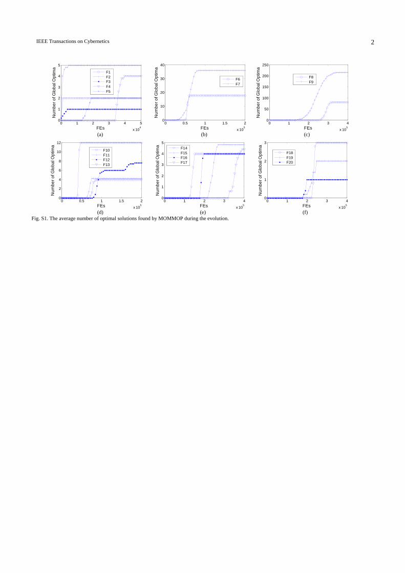
IEEE Transactions on Cybernetics 2

0 1 2 3 4 5

x 104

0

1

2

3

4

5

FEs

Num

ber o

f Glo

bal O

ptim

a

F1F2F3F4F5

0 0.5 1 1.5 2

x 105

0

10

20

30

40

FEs

Num

ber o

f Glo

bal O

ptim

a

F6F7

0 1 2 3 4

x 105

0

50

100

150

200

250

FEs

Num

ber o

f Glo

bal O

ptim

a

F8F9

(a) (b) (c)

0 0.5 1 1.5 2

x 105

0

2

4

6

8

10

12

FEs

Num

ber o

f Glo

bal O

ptim

a

F10F11F12F13

0 1 2 3 4

x 105

0

1

2

3

4

5

FEs

Num

ber o

f Glo

bal O

ptim

a

F14F15F16F17

0 1 2 3 4

x 105

0

1

2

3

FEs

Num

ber o

f Glo

bal O

ptim

a

F18F19F20

(d) (e) (f)

Fig. S1. The average number of optimal solutions found by MOMMOP during the evolution.

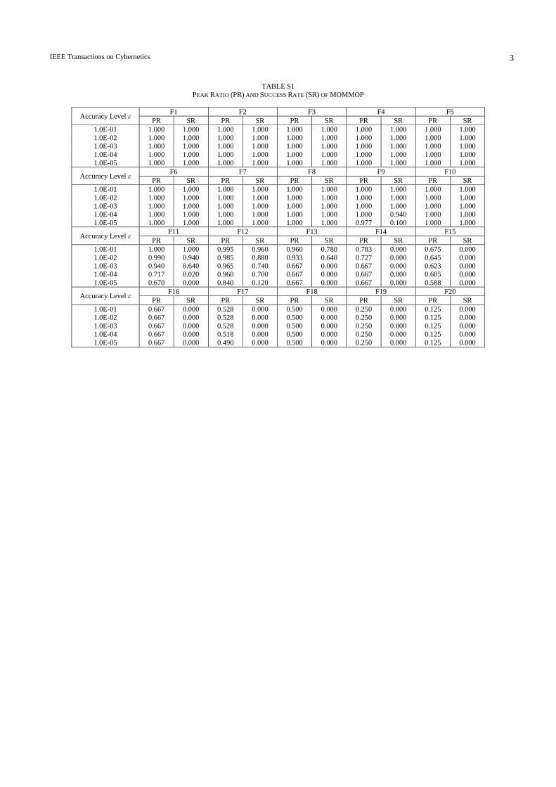
IEEE Transactions on Cybernetics 3

TABLE S1 PEAK RATIO (PR) AND SUCCESS RATE (SR) OF MOMMOP

Accuracy Level ε F1 F2 F3 F4 F5 PR SR PR SR PR SR PR SR PR SR

1.0E-01 1.000 1.000 1.000 1.000 1.000 1.000 1.000 1.000 1.000 1.000 1.0E-02 1.000 1.000 1.000 1.000 1.000 1.000 1.000 1.000 1.000 1.000 1.0E-03 1.000 1.000 1.000 1.000 1.000 1.000 1.000 1.000 1.000 1.000 1.0E-04 1.000 1.000 1.000 1.000 1.000 1.000 1.000 1.000 1.000 1.000 1.0E-05 1.000 1.000 1.000 1.000 1.000 1.000 1.000 1.000 1.000 1.000

Accuracy Level ε F6 F7 F8 F9 F10 PR SR PR SR PR SR PR SR PR SR

1.0E-01 1.000 1.000 1.000 1.000 1.000 1.000 1.000 1.000 1.000 1.000 1.0E-02 1.000 1.000 1.000 1.000 1.000 1.000 1.000 1.000 1.000 1.000 1.0E-03 1.000 1.000 1.000 1.000 1.000 1.000 1.000 1.000 1.000 1.000 1.0E-04 1.000 1.000 1.000 1.000 1.000 1.000 1.000 0.940 1.000 1.000 1.0E-05 1.000 1.000 1.000 1.000 1.000 1.000 0.977 0.100 1.000 1.000

Accuracy Level ε F11 F12 F13 F14 F15 PR SR PR SR PR SR PR SR PR SR

1.0E-01 1.000 1.000 0.995 0.960 0.960 0.780 0.783 0.000 0.675 0.000 1.0E-02 0.990 0.940 0.985 0.880 0.933 0.640 0.727 0.000 0.645 0.000 1.0E-03 0.940 0.640 0.965 0.740 0.667 0.000 0.667 0.000 0.623 0.000 1.0E-04 0.717 0.020 0.960 0.700 0.667 0.000 0.667 0.000 0.605 0.000 1.0E-05 0.670 0.000 0.840 0.120 0.667 0.000 0.667 0.000 0.588 0.000

Accuracy Level ε F16 F17 F18 F19 F20 PR SR PR SR PR SR PR SR PR SR

1.0E-01 0.667 0.000 0.528 0.000 0.500 0.000 0.250 0.000 0.125 0.000 1.0E-02 0.667 0.000 0.528 0.000 0.500 0.000 0.250 0.000 0.125 0.000 1.0E-03 0.667 0.000 0.528 0.000 0.500 0.000 0.250 0.000 0.125 0.000 1.0E-04 0.667 0.000 0.518 0.000 0.500 0.000 0.250 0.000 0.125 0.000 1.0E-05 0.667 0.000 0.490 0.000 0.500 0.000 0.250 0.000 0.125 0.000

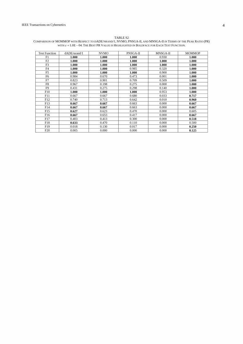
IEEE Transactions on Cybernetics 4

TABLE S2 COMPARISON OF MOMMOP WITH RESPECT TO DADE/NRAND/1, NVMO, PNSGA-II, AND MNSGA-II IN TERMS OF THE PEAK RATIO (PR)

WITH 1.0E 04.ε = − THE BEST PR VALUE IS HIGHLIGHTED IN BOLDFACE FOR EACH TEST FUNCTION.

Test Function dADE/nrand/1 NVMO PNSGA-II MNSGA-II MOMMOP F1 1.000 1.000 1.000 0.930 1.000 F2 1.000 1.000 1.000 1.000 1.000 F3 1.000 1.000 1.000 1.000 1.000 F4 1.000 1.000 0.985 0.320 1.000 F5 1.000 1.000 1.000 0.900 1.000 F6 0.984 0.670 0.473 0.001 1.000 F7 0.823 0.901 0.709 0.509 1.000 F8 0.967 0.198 0.275 0.000 1.000 F9 0.431 0.275 0.298 0.140 1.000 F10 1.000 1.000 1.000 0.953 1.000 F11 0.667 0.667 0.680 0.033 0.717 F12 0.740 0.713 0.642 0.010 0.960 F13 0.667 0.667 0.663 0.000 0.667 F14 0.667 0.667 0.663 0.000 0.667 F15 0.627 0.623 0.470 0.000 0.605 F16 0.667 0.653 0.417 0.000 0.667 F17 0.403 0.413 0.300 0.000 0.518 F18 0.633 0.470 0.110 0.000 0.500 F19 0.018 0.130 0.017 0.000 0.250 F20 0.005 0.000 0.000 0.000 0.125

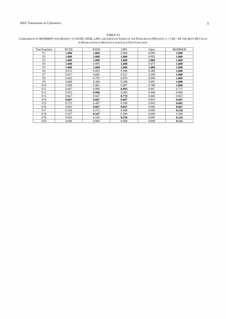
IEEE Transactions on Cybernetics 5

TABLE S3 COMPARISON OF MOMMOP WITH RESPECT TO NCDE, NSDE, LIPS, AND R2PSO IN TERMS OF THE PEAK RATIO (PR) WITH 1.0E 04.ε = − THE BEST PR VALUE

IS HIGHLIGHTED IN BOLDFACE FOR EACH TEST FUNCTION.

Test Function NCDE NSDE LIPS r2pso MOMMOP F1 1.000 1.000 0.000 0.000 1.000 F2 1.000 1.000 1.000 0.992 1.000 F3 1.000 1.000 1.000 1.000 1.000 F4 1.000 0.995 1.000 0.670 1.000 F5 1.000 1.000 1.000 1.000 1.000 F6 0.972 0.993 0.998 0.388 1.000 F7 0.917 0.685 0.527 0.509 1.000 F8 0.062 0.793 0.876 0.000 1.000 F9 0.668 0.384 0.268 0.091 1.000 F10 0.998 0.981 0.987 0.788 1.000 F11 0.667 0.990 0.993 0.667 0.717 F12 0.053 0.990 0.960 0.448 0.960 F13 0.667 0.667 0.770 0.660 0.667 F14 0.667 0.667 0.667 0.003 0.667 F15 0.373 0.497 0.590 0.003 0.605 F16 0.663 0.667 0.667 0.000 0.667 F17 0.250 0.275 0.498 0.000 0.518 F18 0.357 0.547 0.500 0.000 0.500 F19 0.020 0.243 0.250 0.000 0.250 F20 0.000 0.000 0.000 0.000 0.125

IEEE Transactions on Cybernetics 6

TABLE S4 COMPARISON OF MOMMOP WITH RESPECT TO MOBIDE AND BMPGA IN TERMS OF THE PEAK RATIO (PR). THE BEST PR VALUE IS HIGHLIGHTED IN

BOLDFACE FOR EACH TEST FUNCTION.

Test Function The niche radius r ε MOBiDE BMPGA MOMMOP F1 0.5 1E-06 1.000 0.750 1.000 F2 0.01 1E-06 1.000 0.928 1.000 F3 0.01 1E-06 1.000 1.000 1.000 F4 0.5 5E-04 1.000 0.835 1.000 F5 0.5 1E-05 1.000 0.620 1.000 F6 0.2 5E-02 0.967 0.762 1.000 F7 0.2 1E-03 0.983 0.882 1.000 F9 0.1 1E-03 0.814 0.563 1.000

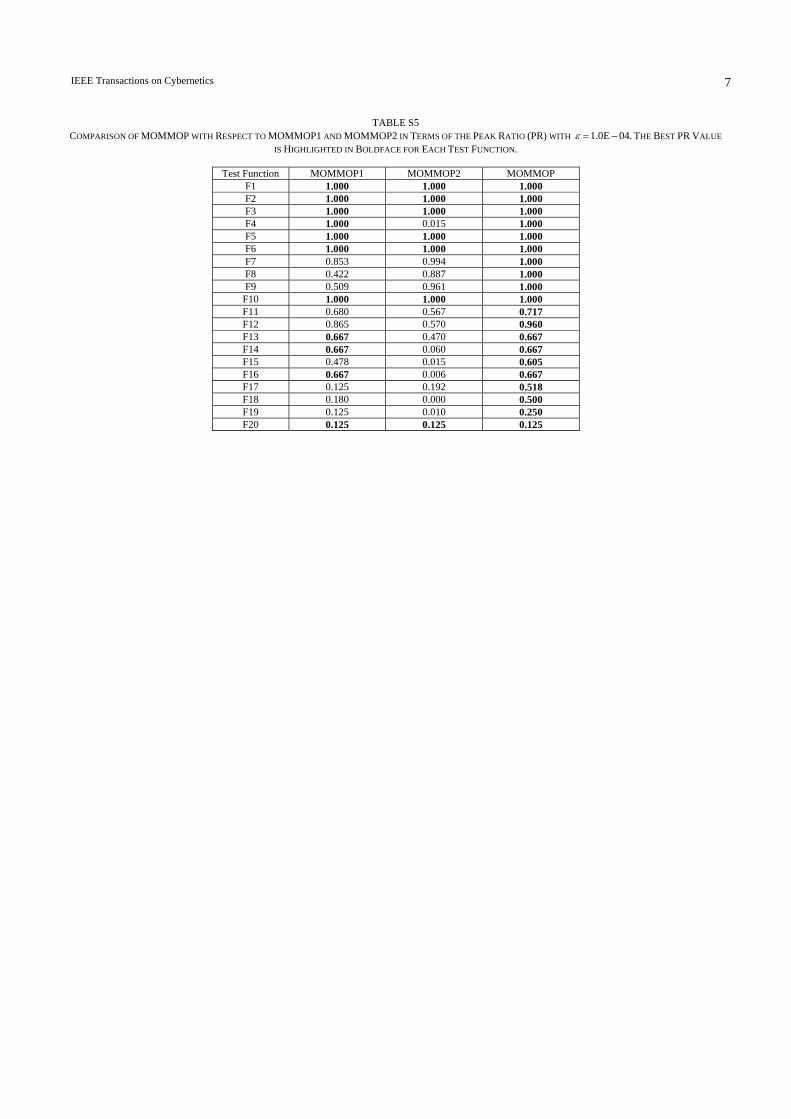
IEEE Transactions on Cybernetics 7

TABLE S5 COMPARISON OF MOMMOP WITH RESPECT TO MOMMOP1 AND MOMMOP2 IN TERMS OF THE PEAK RATIO (PR) WITH 1.0E 04.ε = − THE BEST PR VALUE

IS HIGHLIGHTED IN BOLDFACE FOR EACH TEST FUNCTION.

Test Function MOMMOP1 MOMMOP2 MOMMOP F1 1.000 1.000 1.000 F2 1.000 1.000 1.000 F3 1.000 1.000 1.000 F4 1.000 0.015 1.000 F5 1.000 1.000 1.000 F6 1.000 1.000 1.000 F7 0.853 0.994 1.000 F8 0.422 0.887 1.000 F9 0.509 0.961 1.000 F10 1.000 1.000 1.000 F11 0.680 0.567 0.717 F12 0.865 0.570 0.960 F13 0.667 0.470 0.667 F14 0.667 0.060 0.667 F15 0.478 0.015 0.605 F16 0.667 0.006 0.667 F17 0.125 0.192 0.518 F18 0.180 0.000 0.500 F19 0.125 0.010 0.250 F20 0.125 0.125 0.125

IEEE Transactions on Cybernetics 8

TABLE S6 COMPARISON OF MOMMOP WITH VARYING DISTANCE PARAMETER IN TERMS OF THE PEAK RATIO (PR) WITH 1.0E 04.ε = − THE BEST PR VALUE IS

HIGHLIGHTED IN BOLDFACE FOR EACH TEST FUNCTION.

Test Function 0.001 (MOMMOP_dp1) 0.005 (MOMMOP_dp2) 0.01 (MOMMOP_dp3) 0.05 (MOMMOP_dp4) F1 1.000 1.000 1.000 1.000 F2 1.000 1.000 1.000 1.000 F3 1.000 1.000 1.000 0.903 F4 0.305 1.000 1.000 0.975 F5 1.000 1.000 1.000 1.000 F6 1.000 1.000 1.000 0.413 F7 1.000 1.000 1.000 0.690 F8 1.000 1.000 1.000 0.333 F9 0.998 0.999 1.000 0.713 F10 1.000 1.000 1.000 1.000 F11 0.696 0.710 0.717 0.706 F12 0.952 0.948 0.960 0.932 F13 0.667 0.670 0.667 0.667 F14 0.667 0.667 0.667 0.667 F15 0.557 0.640 0.605 0.602 F16 0.667 0.667 0.667 0.667 F17 0.412 0.490 0.518 0.395 F18 0.453 0.500 0.500 0.500 F19 0.167 0.250 0.250 0.255 F20 0.125 0.125 0.125 0.125

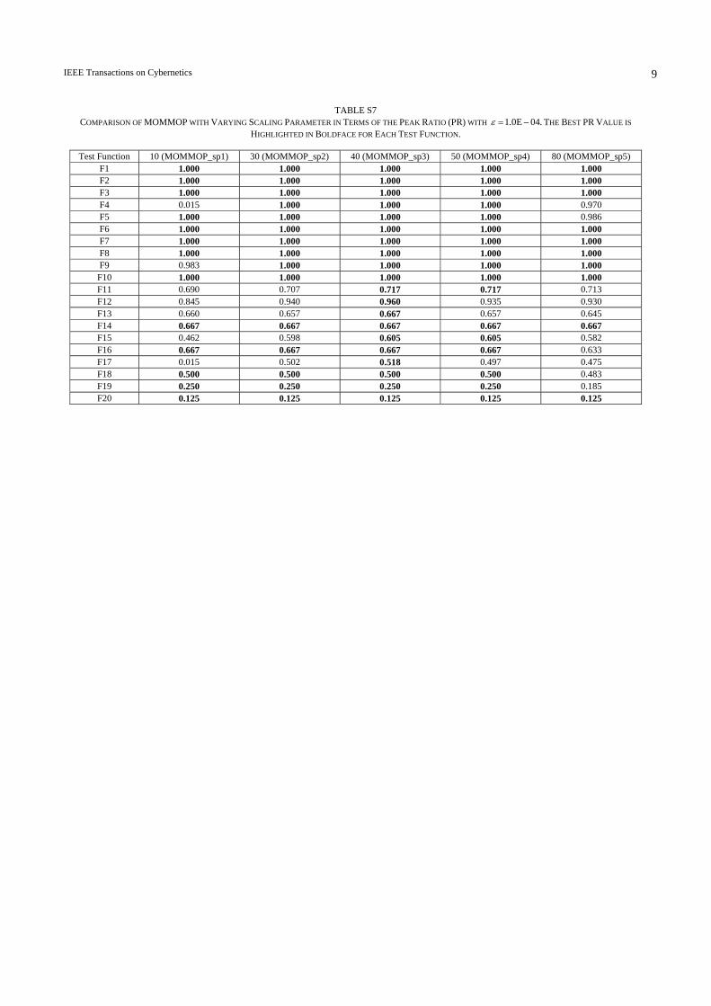
IEEE Transactions on Cybernetics 9

TABLE S7 COMPARISON OF MOMMOP WITH VARYING SCALING PARAMETER IN TERMS OF THE PEAK RATIO (PR) WITH 1.0E 04.ε = − THE BEST PR VALUE IS

HIGHLIGHTED IN BOLDFACE FOR EACH TEST FUNCTION.

Test Function 10 (MOMMOP_sp1) 30 (MOMMOP_sp2) 40 (MOMMOP_sp3) 50 (MOMMOP_sp4) 80 (MOMMOP_sp5) F1 1.000 1.000 1.000 1.000 1.000 F2 1.000 1.000 1.000 1.000 1.000 F3 1.000 1.000 1.000 1.000 1.000 F4 0.015 1.000 1.000 1.000 0.970 F5 1.000 1.000 1.000 1.000 0.986 F6 1.000 1.000 1.000 1.000 1.000 F7 1.000 1.000 1.000 1.000 1.000 F8 1.000 1.000 1.000 1.000 1.000 F9 0.983 1.000 1.000 1.000 1.000 F10 1.000 1.000 1.000 1.000 1.000 F11 0.690 0.707 0.717 0.717 0.713 F12 0.845 0.940 0.960 0.935 0.930 F13 0.660 0.657 0.667 0.657 0.645 F14 0.667 0.667 0.667 0.667 0.667 F15 0.462 0.598 0.605 0.605 0.582 F16 0.667 0.667 0.667 0.667 0.633 F17 0.015 0.502 0.518 0.497 0.475 F18 0.500 0.500 0.500 0.500 0.483 F19 0.250 0.250 0.250 0.250 0.185 F20 0.125 0.125 0.125 0.125 0.125