298 IEEE TRANSACTIONS ON CYBERNETICS, VOL. 46, NO. 1

298 IEEE TRANSACTIONS ON CYBERNETICS, VOL. 46, NO. 1, JANUARY 2016

Pairwise Constraint-Guided Sparse Learningfor Feature Selection

Mingxia Liu and Daoqiang Zhang

Abstract—Feature selection aims to identify the most informa-tive features for a compact and accurate data representation.As typical supervised feature selection methods, Lasso and itsvariants using L1-norm-based regularization terms have receivedmuch attention in recent studies, most of which use class labelsas supervised information. Besides class labels, there are othertypes of supervised information, e.g., pairwise constraints thatspecify whether a pair of data samples belong to the sameclass (must-link constraint) or different classes (cannot-linkconstraint). However, most of existing L1-norm-based sparselearning methods do not take advantage of the pairwise con-straints that provide us weak and more general supervisedinformation. For addressing that problem, we propose a pairwiseconstraint-guided sparse (CGS) learning method for feature selec-tion, where the must-link and the cannot-link constraints are usedas discriminative regularization terms that directly concentrateon the local discriminative structure of data. Furthermore, wedevelop two variants of CGS, including: 1) semi-supervised CGSthat utilizes labeled data, pairwise constraints, and unlabeleddata and 2) ensemble CGS that uses the ensemble of pairwiseconstraint sets. We conduct a series of experiments on a num-ber of data sets from University of California-Irvine machinelearning repository, a gene expression data set, two real-worldneuroimaging-based classification tasks, and two large-scaleattribute classification tasks. Experimental results demonstratethe efficacy of our proposed methods, compared with severalestablished feature selection methods.

Index Terms—Feature selection, L1-norm, pairwise constraint,sparse learning.

Manuscript received August 31, 2014; revised December 2, 2014 andFebruary 3, 2015; accepted February 6, 2015. Date of publication July 6, 2015;date of current version December 14, 2015. This work was supported in partby the National Natural Science Foundation of China under Grant 61422204and Grant 61473149, in part by the Jiangsu Natural Science Foundationfor Distinguished Young Scholar of China under Grant BK20130034, inpart by the Specialized Research Fund for the Doctoral Program ofHigher Education under Grant 20123218110009, in part by the NanjingUniversity of Aeronautics and Astronautics Fundamental Research Fundsunder Grant NE2013105, and in part by the Jiangsu Natural ScienceFoundation of China under Grant BK20130813. This paper was recommendedby Associate Editor D. Tao. (Corresponding author: Daoqiang Zhang.)

M. Liu is with the School of Computer Science and Technology, NanjingUniversity of Aeronautics and Astronautics, Nanjing 210016, China, and alsowith the School of Information Science and Technology, Taishan University,Taian 271021, China.

D. Zhang is with the School of Computer Science and Technology, NanjingUniversity of Aeronautics and Astronautics, Nanjing 210016, China (e-mail:[email protected]).

This paper has supplementary downloadable multimedia material availableat http://ieeexplore.ieee.org provided by the authors. This includes a PDF file,which contains additional results of classification experiments as well as addi-tional results using different parameters and constraint numbers. This materialis 629 KB in size.

Color versions of one or more of the figures in this paper are availableonline at http://ieeexplore.ieee.org.

Digital Object Identifier 10.1109/TCYB.2015.2401733

I. INTRODUCTION

IN MANY machine learning and data mining applications,numerous features can be extracted, and sometimes the

feature dimension is even higher than the number ofdata points [1], [2]. Such high dimensional features not onlyconsume more computation and storage resources, but alsomay degrade the performances of learning algorithms, which istypically referred as “the curse of dimensionality” [3]. Featureselection addresses this issue by selecting the most informa-tive features for a compact and accurate data representation,and has been proven effective in reducing feature dimen-sionality, improving learning performances and facilitatingdata understanding [4]–[7].

According to the different use of supervised information,existing feature selection methods can be categorized into threegroups, i.e., supervised, unsupervised, and semi-supervisedones [3], [7]–[11]. In the literature, most of supervised andsemi-supervised feature selection methods use class labels assupervised information, while class labels are usually lim-ited or expensive to be obtained. For example, in computervision applications, it seems to be impossible to obtain enoughlabeled data to cover all object classes, especially when thereis tens of thousands of categories [12], [13]. Actually, besidesclass labels, there are other types of supervised informa-tion, e.g., pairwise constraints that specify whether a pairof samples belong to the same class (must-link constraints)or different classes (cannot-link constraints) [14]. Comparedwith class labels that require to have detailed informationabout the category of sample, pairwise constraints simplymention for some pairs of samples that they are similaror dissimilar [15]–[17]. Currently, such kinds of constraintshave been widely used in several fields of machine learning,such as distance metric learning [15]–[18], semi-supervisedclustering [19]–[22], dimension reduction [23], [24], andfeature selection [25]–[28]. Especially, several pairwiseconstraints-based feature selection studies have shown thatusing only a small amount of pairwise constraints can achievecomparable performance to those given by supervised featureselection methods using full class labels [25], [27].

On the other hand, Lasso and its variants have receivedincreasing attention in feature selection domain, by usingthe L1-norm-based regularization terms to encourage spar-sity among feature weights [29]–[31]. In the literature,L1-norm-based sparse learning methods have been usedin various real-world applications, such as neuroimagingclassification [32], object categorization [33], and dictionarylearning [34]. However, to the best of our knowledge, most

2168-2267 c© 2015 IEEE. Personal use is permitted, but republication/redistribution requires IEEE permission.See http://www.ieee.org/publications_standards/publications/rights/index.html for more information.

LIU AND ZHANG: PAIRWISE CGS LEARNING FOR FEATURE SELECTION 299

TABLE ILIST OF IMPORTANT NOTATION

existing L1-norm-based sparse learning methods use only classlabels as supervised information, and do not take advantageof pairwise constraints that provide us weak and more generalsupervised information.

For addressing this problem, we propose a pairwiseconstraint-guided sparse (CGS) learning method for featureselection, where the must-link and the cannot-link con-straints are used as discriminative regularizers that directlyconcentrated on the local discriminative structure of data.Furthermore, we develop two variants to the proposed CGSmethod. The first one is the semi-supervised CGS (SCGS)method that uses labeled data, pairwise constraints, and unla-beled data. The second one is the ensemble CGS (ECGS)method that uses the ensemble of pairwise constraint setsother than a single constraint set. We conduct a series ofexperiments on a number of data sets from University ofCalifornia-Irvine (UCI) machine learning repository, a geneexpression data set, and two real-world neuroimaging-basedclassification tasks. Experimental results validate the efficacyof our proposed methods.

The major contributions of this paper are threefold. First, wepropose a novel pairwise CGS feature selection method, whichexploits the pairwise constraint-based regularizers to reflectthe local discriminative structure of data. Second, we developa SCGS model by using labeled data, pairwise constraints, andunlabeled data, and an ECGS method by using an ensembleof multiple pairwise constraint sets. Third, we develop an effi-cient optimization algorithm for solving the proposed problem.

The remainder of this paper is organized as follows.Section II briefly reviews related background knowledge onfeature selection. In Section III, we present the proposed CGSfeature selection method, an efficient optimization algorithm,a semi-supervised variant of CGS, and an ensemble variant ofCGS. Section IV provides the experimental results and anal-ysis on a number of data sets, by comparing the proposedmethods with several established feature selection methods.In Section V, we first discuss the influences of the parame-ters and the constraint number on the performances of CGS,and then compare our proposed methods with several sparseclassifiers. Section VI concludes this paper.

II. BACKGROUND

In this section, we first briefly introduce several well-knownsupervised and unsupervised feature selection methods,

including variance [35], Laplacian score (LS) [36], and Fisherscore (FS) [35]. Then, we introduce recent work on pairwiseconstraint-based feature selection. Finally, we present relatedwork on L1-norm-based sparse feature selection.

A. Supervised and Unsupervised Feature Selection

Denote the training data set as X = {xi}Ni=1 (xi ∈ Rd), where

N is the number of data points and d is the feature dimen-sion. Let fri denote the rth feature of sample xi. Define µr =1/N

∑Ni=1 fri as the mean of the rth feature f r. For supervised

learning problems, class labels are given in Y = {yi}Ni=1, yi ∈

{1, . . . , P}, where P is the class number and Np denotes thenumber of data points belonging to the pth class. For conve-nience, we list important notation used in this paper in Table I.

As a simple unsupervised evaluation of features, varianceutilizes the variance along a feature dimension to reflectthe feature’s representative power for the original data. Thevariance of the rth feature denoted as Varr, which should bemaximized, is computed as follows [35]:

Varr = 1

N

N∑

i=1

( fri − µr)2. (1)

As another unsupervised method, LS prefers featureswith larger variances as well as stronger locality preservingability. It can be regarded as the extension of the Laplacianeigenmaps [37] for feature selection. The key assumption inLS is that the data points from the same class should be closeto each other. The LS of the rth feature denoted as LSr, whichshould be minimized, is computed as follows [36]:

LSr =∑

i,j

(fri − frj

)2Sij

∑i ( fri − μr)

2Dii. (2)

Here, D is a diagonal matrix with element Dii = ∑Nj=1 Sij,

and Sij represents the neighborhood relationship betweensamples xi and xj defined as follows:

Sij =⎧⎨

⎩e−‖xi−xj‖2

σ2 , if xi and xj are k nearest neighbors0, otherwise

(3)

where σ is a width parameter to be set.FS is a supervised method using full class labels. It seeks

features that can maximize the distance of data points between


different classes and minimize the distance of data pointswithin the same class simultaneously. Let µ

pr and f p

r be themean and the feature vector of class p corresponding to therth feature. The FS of the rth feature (i.e., FSr) is computedas follows [35]:

FSr =∑P

p=1 Np(µ

pr − µr

)2

∑Pp=1

∑Npi=1

(f pri − µ

pr)2

. (4)

B. Pairwise Constraints-Based Feature Selection

In practice, obtaining class labels is usually expensive,and, thus, the amount of labeled training data is sometimesvery limited. Therefore, we are often faced with the socalled “small labeled-sample problem” in many real-worldapplications [3]. For addressing that problem, pairwise con-straints (also called side information) arise naturally in manytasks [15], [19], [22], [38]. For example, in the domain ofimage retrieval [39], considering pairwise constraints is morepractical than trying to obtain class labels, because true classlabels may be unknown but it is easier for users to specifywhether some pairs of data samples belong to the same class(must-link constraint) or different classes (cannot-link con-straint), i.e., similar or dissimilar. On the other hand, pairwiseconstraints can be derived from labeled data but not vice versa.In addition, pairwise constraints can be given in advance orgenerated from class labels. Given N labeled samples, we cangenerate approximately N2 pairwise constraints. For these rea-sons, pairwise constraints have been widely used in machinelearning fields.

Recently, researchers developed various feature selec-tion methods by using pairwise constraints. For example,Zhang et al. [25] proposed the so called constraint score (CS)to evaluate the goodness of features by using pairwise con-straints. To be specific, CS utilizes M = {(xi, xj)| xi and xj

belong to the same class} containing pairwise must-link con-straints and C = {(xi, xj)| xi and xj belong to different classes}containing pairwise cannot-link constraints as the supervisedinformation. The CSs of the rth feature (denoted as CSr) arecomputed in the following form [25]:

CSr =∑

(xi,xj)∈M

(fri − frj

)2 − λ∑

(xi,xj)∈C

(fri − frj

)2 (5)

where λ is a parameter to balance the two terms in (5). Ithas been shown that CS, with only a small amount of pair-wise constraints, can achieve comparable performance to fullysupervised feature selection methods [25].

In addition, Kalakech et al. [27] developed a semi-supervised CS by using both pairwise constraints and localproperties of the unlabeled data. To alleviate the bias intro-duced by the selection of appropriate pairwise constraint sets,Sun and Zhang [26] proposed a bagging CS method to boostthe performance of original CS.

C. L1-Norm-Based Sparse Feature Selection

In the literature, sparse learning attracts much attentionin pattern recognition and machine learning domains, amongwhich Lasso is one of the most widely used ones [29].

Generally, Lasso is a penalized least squares method with theL1-norm penalty on the weight vector (i.e., w ∈ R

d), and itsobjective function is defined as follows:

minw

N∑

i=1

(yi − wTxi

)2

s.t. ‖w‖1 ≤ t (6)

where t ≥ 0 is a tuning parameter to control the amount ofshrinkage applied to the estimate w. Due to the sparsity natureof L1-norm, the Lasso method can perform feature selectionand regression/classification simultaneously.

Following [29], researchers have developed variousL1-norm-based sparse learning methods (e.g., elastic net [40],group Lasso [31], and fused Lasso [30]). These methods havebeen widely used in dimension reduction [13], [41], imagingannotation [42], [43], and face recognition [33]. It is worthnoting that most existing L1-norm-based feature selectionmethods only use class labels as supervised information, whileclass labels may be limited or expensive to be obtained in prac-tice. To the best of our knowledge, no previous L1-norm-basedsparse learning research has tried to perform feature selectionby exploiting pairwise constraints as supervised information.

III. PAIRWISE CGS LEARNING

In this section, we first propose a pairwise CGS learningmethod for feature selection, where pairwise constraints areused as discriminative regularization terms. Then, we presentan efficient optimization algorithm for solving the proposedproblem. In addition, we further extend our proposed CGSmethod into a semi-supervised variant called SCGS, and anensemble variant denoted as ECGS.

A. Proposed CGS Method

Denote N as the size of data points, X = {xi}Ni=1 as data set

with class labels Y = {yi}Ni=1. Let w ∈ R

d denote the weightvector, while M and C represent the must-link constraints setand the cannot-link constraints set, respectively. Intuitively,in the mapping space, data points from the must-link con-straint set should be close to each other, and those fromthe cannot-link constraint set should be as far as possible.Accordingly, the proposed sparse learning model using bothpairwise constraints and class labels is defined as follows:

minw

1

2

N∑

i=1

loss(xi, yi, F) + λ1

2(U − αV) + λ2‖w‖1 (7)

where U = ∑(xi,xj)∈M (wTxi − wTxj)

2, V =

∑(xi,xj)∈C (wTxi − wTxj)

2, and loss(xi, yi, F) is a gen-

eral loss function. One can use various loss functions, such asleast squares loss and logistic loss. Here, we adopt the leastsquare loss in this paper, i.e., F(xi) = yi − wTxi. The secondterm is used to force the distance between samples involvedin the must-link set to be small (i.e., intraclass compactness),and the distance between samples involved in the cannot-linkset to be large (i.e., interclass separability). Actually, the sec-ond term is a discriminative regularization term that directly


concentrates on the local discriminative structure of data byusing the underlying supervised information conveyed bythe must-link and the cannot-link constraints [44], [45]. Theparameter α is the regularization parameter that regulates therelative significance of the intraclass compactness and theinterclass separability. The last term is the L1-norm-basedregularization term used to generate sparse coefficients fordifferent features.

Let SM and SC denote similarity matrices defined on thepairwise cannot-link constraint set and the cannot-link con-straint set, respectively. Here, SM and SC are defined asfollows:

SMij =

{1, if

(xi, xj

) ∈ M0, otherwise

(8)

SCij =

{1, if

(xi, xj

) ∈ C0, otherwise.

(9)

Let DM and DC denote two diagonal matrices, whereDM

ii = ∑Nj=1 SM

ij and DCii = ∑N

j=1 SCij . Then, we can com-

pute the must-link Laplacian matrix LM = DM − SM, and thecannot-link Laplacian matrix LC = DC−SC [46]. Accordingly,the regularization terms defined on the must-link constraintsand the cannot-link constraints in (8) can be rewritten as

∑

(xi,xj)∈M

(wTxi − wTxj

)2 =∑

i,j

(wTxi − wTxj

)2SM

ij

= 2wTXTLMXw (10)

and∑

(xi,xj)∈C

(wTxi − wTxj

)2 =∑

i,j

(wTxi − wTxj

)2SC

ij

= 2wTXTLCXw. (11)

By employing the least square loss as well as (10) and (11),we can reformulate the proposed model defined in (7) asfollows:

minw

1

2‖Y − Xw‖2

2 + λ1wTXT(

LM − αLC)

Xw + λ2‖w‖1.

(12)

In addition, to further preserve the structure informationof original data, we introduce a manifold regularization term,which is as follows:

∑

i,j

(wTxi − wTxj

)2Sij = 2wTXTLXw (13)

where L denotes the Laplacian matrix on original data, andD is a diagonal matrix with element Dii = ∑N

j=1 Sij, whilethe similarity matrix S is defined in (3). By introducing themanifold regularization term into (12), we have the followingobjective function:

minw

1

2‖Y − Xw‖2

2 + λ1wTXT(

LM − αLC)

Xw

+ λ2‖w‖1 + λ3wTXTLXw (14)

where the first term is the empirical loss on the training data,and the second term is a discriminative regularization term to

Algorithm 1 Learning Algorithm Based on CGS

Input: The training data X = {xi}Ni=1; The class labels

Y = {yi}Ni=1; The number of must-link constraints NM;

The number of cannot-link constraints NC; The learner �.Initialize: The parameters for CGS, i.e., λ1, λ2, λ3 and α.1: Generate the must-link constraints set M and the

cannot-link constraint set C;2: Calculate the similarity matrices SM, SC and S using

Eqs. (8), (9) and (3), respectively; Compute thecorresponding Laplacian matrices LM, LC and L;

3: Compute the optimal solution w of (14);4: Construct the feature subset G by selecting features with

nonzero coefficients of w;5: Call the learner �, providing it with the training data set

{xGi , yi}N

i=1 where xGi denotes the sample xi with features

in G.

Output: The hypothesis h: ϕTxG → Y

preserve the local discriminative structure of data conveyed bypairwise constraints. The last two terms are the L1-norm-basedregularizer and the manifold regularization terms,respectively.

The model defined in (14) is called pairwise CGS featureselection method in this paper. Without the manifold regu-larization term (i.e., λ3 = 0) in (14), the proposed model iscalled CGS without manifold regularization term (CGSwm).Let λ1 = 0 and λ3 = 0, and we find that the proposed CGSmethod is equivalent to the Lasso formulation defined in (6).Finally, with λ1 = 0, the proposed CGS model is equivalentto the Laplacian Lasso (LapLasso) model [47]. The learningalgorithm based on our proposed CGS approach is given inAlgorithm 1.

Now, we analyze the computational complexity ofAlgorithm 1. There are three main steps in Algorithm 1.

1) Step 1: Generates the must-link and the cannot-link pairwise constraints, requiring O(NM + NC)operations.

2) Step 2: Calculates three similarity matrices requiringO(N2 + N2

M + N2C) operations.

3) Step 3: Computes w using Algorithm 2 that needsO(1/Q2) operations given the iteration number Q.

Hence, the overall computational complexity of Algorithm 1is O(N2 + N2

M + N2C).

B. Optimization Algorithm

Now, we introduce an efficient optimization algorithm forsolving the objective function of CGS defined in (14). It isstraightforward to verify that the proposed objective func-tion is convex but nonsmooth because of the nonsmoothL1-norm regularization term. The basic idea to solve the prob-lem is to use a smooth function to approximate the originalnonsmooth objective function, and then solve the former byutilizing some off-the-shelf fast algorithms. In this paper, weresort to the widely used accelerated proximal gradient (APG)method [48], [49] to solve the proposed objective functionin (14). To be specific, we first separate the objective function


(a) (b)

Fig. 1. Convergence of the objective function value on (a) Habermanand (b) ionosphere data sets.

in (14) to the smooth part

f (w) = 1

2‖Y − Xw‖2

2 + λ1wTXT(

LM − αLC)

Xw

+ λ3wTXTLXw (15)

and the nonsmooth part

h(w) = λ2‖w‖1. (16)

To approximate the composite function f (w) + h(w), wefurther construct the following function:

�T,wj(w) = f(wj

) + ⟨w − wj,∇f

(wj

)⟩

+ T

2

∥∥w − wj

∥∥2

2 + h(w) (17)

where ∇f (wj) denotes the gradient of f (w) at the point wj,and T is the step size that can be determined by line search,e.g., the Armijo–Goldstein rule [50]. Finally, the update stepof AGP algorithm is defined as follows:

wj+1 = minw

1

2

∥∥w − vj

∥∥2

2 + 1

Th(w) (18)

where the term vj = wj − 1/T∇f (wj).The key of AGP algorithm is deciding how to solve the

update step efficiently. Liu and Ye [51] showed that this prob-lem can be decomposed into several separate sub-problems.Thus, we can obtain the analytical solutions of these sub-problems easily. In addition, to achieve faster convergence rate,the accelerated gradient method is based on two sequences{wj} and {gj}, where wj is the sequence of approximate solu-tions and {gj} is the sequence of search points [48]. The searchpoint gj is the affine combination of wj−1 and wj as

gj = wj + γj(wj − wj−1

)(19)

where γj is a properly chosen coefficient. The detailed pro-cesses are given in Algorithm 2.

For a fixed Q (i.e., the maximum iteration), the APG algo-rithm for the problem in (14) has O(1/Q2) asymptoticalconvergence rate. In Fig. 1, we plot the change of the objec-tive function values versus iteration number on the Habermanand the ionosphere data sets from UCI machine learningrepository [52]. From Fig. 1, one can see that the values of theobjective function value decreases rapidly within ten iterations,illustrating the fast convergence of Algorithm 2.

Algorithm 2 Optimization Algorithm for CGS

Input: The training data X = {xi}Ni=1; The class labels

Y = {yi}Ni=1; The Laplacian matrices LM, LC and L;

Initialize: The maximum iteration number Q; The stepsize T0; The parameters for CGS, i.e., λ1, λ2 and λ3.

1: Let w0 = w1 = 0, β0 = 1, and T = T0;2: for j = 1 to Q do3: Set γj = (1−βj−1)βj

βj−1, and compute gj according to (19);

4: Find the smallest T = Tj−1, 2Tj−1, . . . such that

f(wj+1

) + h(wj+1

) ≤ �T,gj(w)

where wj+1 is computed using (18);

5: Set Tj = T and βj+1 = 1+√

1+4β2j

2 .6: end forOutput: wj

C. Proposed SCGS Method

The proposed CGS method is supervised, which requiresfull class labels. However, in many real-world applications,labeled data is usually hard or expensive to be obtained,while unlabeled data and pairwise constraints may be easierto be obtained [20]. In such cases, semi-supervised learningmethods are shown helpful to promote the performances ofa learning model [10], [21], [22]. In this section, we extendour proposed CGS model to a semi-supervised variant.

Define a diagonal matrix A ∈ RN×N to indicate the labeleddata, i.e., Aii = 0 if the class label of sample xi is unknownand Aii = 1 otherwise. The objective function of our proposedSCGS model (denoted as SCGS) is as follows:

minw

1

2‖A(Y − Xw)‖2

2 + λ1wTXT(

LM − αLC)

Xw

+ λ2‖w‖1 + λ3wTXTLXw (20)

where LM, LC, and L denote Laplacian matrices definedon the must-link constraint set, the cannot-link constraint set,and the whole training data, respectively. In (20), the first termis the empirical loss on labeled data, the second term is a dis-criminant regularization term focusing on the local structureof data reflected by pairwise constraints, and the last term isan unsupervised estimation on intrinsic geometry distributionof the original data. Similarly to CGS and CGSwm, the SCGSmethod without the last Laplacian regularization term in (20)is called SCGSwm in this paper.

D. ECGS Method

In [25]–[27], it has been shown that the selection of pair-wise constraints has a significant impact on the performancesof pairwise constraint-based methods. That is, different sets ofpairwise constraints often result in highly unstable results onthe same data set. However, deciding how to select the appro-priate pairwise constraints set for specific tasks is an openproblem [53]. Recently, ensemble-based methods have beenproposed for addressing that problem [26], [54], [55]. Inspiredby those methods, instead of making efforts on finding a singleproper pairwise constraint set, we extend our proposed CGS


Fig. 2. Flowchart of the proposed ECGS method that uses an ensem-ble of multiple pairwise constraint sets. Note NE is the number of pairwiseconstraint sets.

Fig. 3. Relationship of the proposed CGS method and other related methods.

approach by using the ensemble of multiple pairwise constraintsets. The flowchart of the proposed ECGS method is shownin Fig. 2.

As shown in Fig. 2, we first generate multiple pair-wise constraint sets. Specifically, we randomly select pairsof samples from the training data, and then generate themust-link or cannot-link constraints are created depending onwhether the underlying classes of two samples are the sameor different. Then, we execute the proposed CGS algorithmon those individual constraint sets, through which multi-ple feature subsets can be determined. Afterwards, differentindividual learners are constructed based on those featuresubsets. Finally, we adopt the majority voting strategy forthe construction of classifier ensemble, because it is a verysimple as well as widely used method for the fusion ofmultiple classifiers [26]. The ensemble versions of our pro-posed CGS and CGSwm methods are denoted as ECGS andECGSwm, respectively. It is worth noting that the ensem-ble method we used here is to employ multiple learners andcombine their prediction [54], which is different from multi-view learning that mainly focuses on learning from multiviewfeatures [42], [56].

From the above analysis, we can see that our proposed CGSmethod can be regarded as a unified framework for various fea-ture selection methods. The relationship between CGS methodand the other related methods is shown in Fig. 3.

IV. EXPERIMENTS

In this section, we first introduce the data sets used in ourexperiments, and then present the experiment design and theexperimental results.

A. Data Sets

First, we evaluate our proposed methods (i.e., CGS,CGSwm, ECGS, and ECGSwm), on ten data sets from UCImachine learning repository [52], and a high-dimensional geneexpression data set (i.e., colon cancer [57]).

We also perform experiments on attribute classificationtasks on the aYahoo [58] and the ImageNet [59] data sets.The aYahoo data set consists of 1151 images of 2688-Dfeatures and 64 binary attributes [58], and the ImageNetdata set consists of 9600 images with 1550-D features with25 attributes [59]. These attributes describe properties ofobjects in the images, such as color, shape, texture, atomy,and parts. In each attribute classification task, images rep-resented by low-level features are used as input data andthe attributes for all images are regarded as labels. For theaYahoo data set, we use 15 attributes (with relatively bal-anced positive and negative samples) to perform attributeclassification.

In addition, we evaluate our methods on two neuroimaging-based classification tasks using an Alzheimer’s disease (AD)data set, obtained from the AD neuroimaging initiativedatabase (http://adni.loni.usc.edu). This data set have includ-ing 202 subjects with the magnetic resonance imaging (MRI),positron emission tomography (PET), and cerebrospinalfluid (CSF) baseline data. There are three categories ofsubjects, including 51 AD patients, 99 mild cognitive impair-ment (MCI) patients, and 52 normal control (NC). In theexperiments, we perform two classification tasks, includ-ing “AD versus NC” classification and “MCI versus NC”classification. Similar to [32], we first perform preprocessingfor all MR and PET images. Then, for each of the 93 regionof interest (ROI) regions in the labeled MR images, we com-pute the volume of gray matter tissue in that ROI region asa feature. For each subject, we obtain 93 features from the MRimages. For PET images, we use a rigid transformation to alignthem onto its respective MR images of the same subject, andthen compute the average intensity of each ROI in the PETimage as a feature. For each subject, we obtain 93 featuresfrom the MRI image, another 93 features from the PET image,and three features from the CSF biomarkers. Then, we con-catenate these features to form the 189-D representation fora subject. The statistics of data sets used in our experimentsare summarized in Table II.

B. Experiment Design

In the experiments, we compare our proposed methodswith several well-known feature selection methods,including LS [36], FS [35], CS [25], Lasso [29], andLapLasso [47], [60]. The performance of a specific featureselection method is measured by the classification accuracybased on the selected features on the training data. For LS,FS, and CS methods, we first select the first m featuresfrom the ranking list of features generated by correspondingalgorithms, where m is the desired number of selectedfeatures specified as m = {1, 2, . . . , d} in the experiments.Then, we report the highest classification accuracy as well thenumber of selected features for LS, FS, and CS. For Lasso,


TABLE IISTATISTICS OF DATA SETS USED

IN OUR EXPERIMENTS

LapLasso and the proposed methods, the optimal featuresubset is determined through corresponding algorithms, andthe classification results are reported using such fixed featuresubsets. Two classifiers are used to perform classificationtasks. The first one is the K-nearest neighborhood (K-NN)classifier with Euclidean distance and K = 1, and the secondone is a linear support vector machines (SVMs) with thedefault regularization parameters value (i.e., C = 1) [61].

In the supervised classification experiments, we adopt a five-fold cross-validation strategy to compute the mean and thevariance of classification accuracy. To be specific, the orig-inal data set is partitioned into five subsets (each subsetwith roughly equal size), and each time samples within onesubset are successively selected as the testing data whileall the remaining samples in the other four subsets arecombined together as the training data to perform featureselection and to learn corresponding classifiers. The processis repeated for ten times independently to avoid any biasintroduced by the random partitioning of original data inthe cross-validation process. Similarly, in the semi-supervisedclassification experiments, we adopt a fivefold cross-validationstrategy. Specifically, we first partition the original data intoroughly equal five folds, and each time we select one offive subsets as the test data, and the others are used fortraining. For those training data, we randomly select 40%samples as labeled data, and select 40% samples to gen-erate pairwise constraints, while the rest ones are used asunlabeled data. To avoid any bias induced by the random par-titioning of original data, the above process is repeated forten times.

The generation of pairwise constraints is simulated in thefollowing way. First, we randomly select pairs of samplesfrom the training data. Then, the must-link constraints and thecannot-link constraints are created depending on whether theunderlying classes of two samples are the same or different. Toalleviate the bias introduced by the selection of pairwise con-straint sets, following [25], the results achieved by CS and the

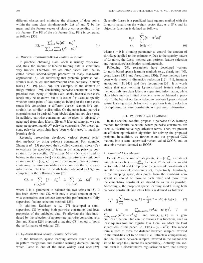
TABLE IIITOP 12 ROIS IDENTIFIED BY OUR PROPOSED CGS

METHOD IN AD VERSUS NC CLASSIFICATION

proposed CGS as well as CGSwm are averaged over 20 runswith different generation of pairwise constraints. For theproposed ECGS and ECGSwm methods, we first generate NE

different must-link and cannot-link constraint sets, and thencreate multiple sets of selected features by using our proposedCGS and CGSwm approaches, respectively. Based on thesefeature subsets, we can train multiple learners through corre-sponding learning algorithms (e.g., SVM and K-NN). Finally,we adopt the majority voting strategy to get a final decisionfor a specific testing sample. In addition, as shown in [26],one can obtain the best classification results with the ensem-ble size NE = 20, and using more than 20 components in theensemble will not further improve the classification results butbring much computational burden. So in our experiments, theensemble size NE (i.e., number of constraint sets) is set as20 empirically.

It has been shown in [25] and [26] that using equal num-bers of must-link and cannot-link constraints achieves betterperformance than using imbalanced constraints in pairwiseconstraint-based methods. Accordingly, for four constraint-based feature selection approaches (including CS, CGS,CGSwm, ECGS, and ECGSwm), we use equal numbers ofmust-link and cannot-link constraints in the experiments. Tobe specific, the numbers of must-link and cannot-link con-straints are set as 20% of the sample size for a specificdata set. For fair comparison, CS and our proposed methods(i.e., CGS, CGSwm, ECGS, and ECGSwm) share the samepool of pairwise constraints.

Following [25], the parameter λ for CS as well as theparameter α for the proposed CGS method are set tobe 0.1 empirically. The regularization parameters λ1, λ2,and λ3 for our proposed CGS method are chosen from{10−6, 10−5, . . . , 100} through fivefold cross-validation on thetraining data. Similarly, the parameters λ1 in Lasso, as wellas λ1 and λ2 in our proposed CGSwm method, are selectedfrom the same range by cross-validation on the training data.The influence of different parameter values on the perfor-mance of our proposed method will be further discussedin Section V.


TABLE IVSUPERVISED CLASSIFICATION RESULTS USING K-NN CLASSIFIER (%)

C. Features Selected by the Proposed Method

To investigate whether the proposed CGS method can selectthe most informative features, we perform the AD versusNC classification on the AD data set to show the featuresselected by our proposed CGS method. Since the selected fea-tures (i.e., ROIs) are different in each cross-validation fold, wechoose those features with the highest selection frequency inall folds as the most informative features. For each selectedfeature, a paired t-test is performed to evaluate its discrimi-native power for identifying AD patients from NCs, throughwhich the p-value between each specific selected feature andclass labels among all training samples can be computed. InTable III, we list the top 12 ROIs selected by our proposedCGS method from all 189 features, as well as correspondingp-values.

From Table III, we can see that the top 12 regions includehippocampal, amygdala, and temporal pole, which are reportedto be very relevant to AD disease in [32] and [55]. Onthe other hand, from Table III, we can see that most ofselected features have small p-values indicating their strongdiscriminative power for distinguishing patients from NCs. Itimplies that our proposed CGS method can effectively find themost informative features.

D. Results of Supervised Classification

We first validate the efficacy of proposed CGS and CGSwmmethods in a supervised problem setting, in comparison toLS, FS, CS, Lasso, and LapLasso. In Table IV, we report theclassification results using K-NN classifier, while the resultsusing SVM are shown in Table SI in the online supplementarymaterials. The meaning of the symbols in the term “a ± b(c)”is as follows: “a” and “b” denote the mean and the varianceof classification accuracies among fivefold cross validation,respectively, while “c” represents the number of selectedfeatures. Note that the best results are shown in boldface.

Fig. 4. Classification results of different supervised feature selection methodson the aYahoo data set using K-NN classifier.

We also perform paired t-test between the accuracy achievedby our proposed CGS method and the accuracy achieved bya compared method. The values in Table IV further markedby “*” indicate that our proposed CGS method achieves sig-nificant improvement than the other methods by paired t-test(with the confidence interval at 95%). In addition, we reportthe mean results of attribute classification using K-NN clas-sifier on the aYahoo data set and the ImageNet data setin Table IV.

From Table IV, we can observe four main points. First, ourproposed CGS and CGSwm methods usually achieve the over-all better performances than the other methods. For example,on the sonar data set, the accuracy achieved by the proposedCGS approach is 94.28%, while the best accuracy of the othermethods is only 92.85% (achieved by LS and FS). Second,in most cases, the numbers of features selected by CGS andCGSwm are less than that of other five methods. In particular,on colon cancer data set, CGS achieves the highest accuracy


(a) (b) (c) (d)

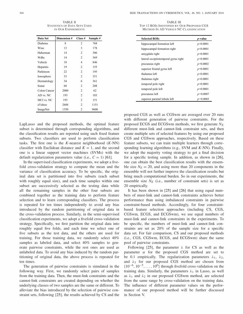
Fig. 5. Classification accuracies versus different numbers of selected features achieved by seven feature selection methods on (a) Haberman, (b) ionosphere,(c) hepatitis, and (d) sonar data sets.

using only two features, while the best result is achieved byFS with eight features. Third, for pairwise constraint-basedmethods, our proposed CGS method consistently performs bet-ter than CS and CGSwm usually outperforms CS. Finally, CGSthat considers both the pairwise constraints and the manifoldinformation is usually superior to CGSwm using only pairwiseconstraints. Similarly, LapLasso that considers the manifoldinformation achieves better results than Lasso in most cases. Itindicates that the structure information is important in guidingthe process of feature selection.

In Fig. 4, we show the results of 15 attribute classificationon aYahoo data set with K-NN classifier, while results withSVM classifier are given in Fig. S1 in the online supplemen-tary materials. At the same time, we also report the attributeclassification results on the ImageNet data set using bothK-NN and SVM classifiers in Figs. S2 and S3, respectively, inthe online supplementary materials. From Figs. 4 and S1–S3,one can observe that our proposed methods (i.e., CGS andCGSwm) usually outperform the other compared methods inmultiple attribute classification tasks. Especially, as shown inFig. 4, in the “Eye” and “Head” classification tasks on theaYahoo data set, CGS achieves much higher accuracy thanthe compared methods.

Furthermore, we investigate the influence of the numberof selected features on the classification results. For LS, FS,and CS, the number of selected features vary from 1 tod according to feature ranking lists obtained by a specificalgorithm. For L1-norm-based methods (i.e., Lasso, LapLasso,CGSwm, and CGS), the parameter for the L1-norm regular-ization term that controls the sparsity of feature coefficients(corresponding to optimal number of selected features) is cho-sen from {10−6, 10−5, . . . , 100} through cross-validation. Theother parameters for CGS (i.e., λ1 and λ3), the parameter λ1for CGSwm, and the parameter λ2 for LapLasso are chosenfrom the same range through cross-validation on the trainingdata. In Fig. 5, we plot the curves of classification accuracyversus different numbers of selected features on four UCIdata sets using K-NN classifier.

From Fig. 5, we can see that our proposed CGS andCGSwm methods achieve the overall best performances usingsmaller number of selected features, in comparison to LS,FS, and CS. Particularly on the Haberman and the ionospheredata sets, CGS, and CGSwm need less than half of features toachieve the best performances. Second, using similar number

of selected features, CGS and CGSwm achieve higher clas-sification accuracies than Lasso and LapLasso in most cases.This conclusion is consistent with the results in Table IV.

E. Results of Semi-Supervised Classification

In this section, we evaluate our proposed SCGS andSCGSwm methods in a semi-supervised problem setting onUCI data sets, in comparison to FS, Lasso, and LapLasso.Note that LapLasso, SCGSwm, and SCGS methods use bothlabeled data and unlabeled data, while FS and Lasso use onlythe labeled data. We report the classification results achievedby different feature selection methods using K-NN in Table V,while the results using SVM classifier are given in Table SIIin the online supplementary materials.

From Table V, we can find that, in most cases, SCGS per-forms better than FS, Lasso, and LapLasso, especially on thehepatitis and the sonar data sets. These results imply that thefeatures selected by SCGS have better discriminative abil-ity compared with those selected by other methods. Recallthe results in Table IV achieved by the proposed supervisedCGS method, and we can find that although a small numberof labeled data are used in the proposed SCGS method, theclassification performances achieved by SCGS only decreaseslightly compared with the results in a full supervised manner.For example, from Tables IV and V, we can clearly seethat the performances of SCGS are similar to those of CGSon diabetes, wine, and Wisconsin diagnostic breast cancer.These results demonstrate that our proposed CGS method caneffectively identify discriminative features in semi-supervisedproblem settings. The underlying reason may be that the dis-advantage of lacking enough labeled data can be compensatedby the information conveyed by pairwise constraints in theproposed SCGS method.

F. Results of ECGS

We then compare our proposed CGS and CGSwm methodswith their ensemble counterparts, i.e., ECGS and ECGSwm,respectively. The classification results using the K-NN clas-sifier are given in Fig. 6, and the results using the SVMclassifier are shown in Fig. S4 in the online supplemen-tary materials. From Fig. 6, we can see that, in most cases,the proposed ECGS method using the ensemble of pair-wise constraint sets outperforms its traditional counterpart


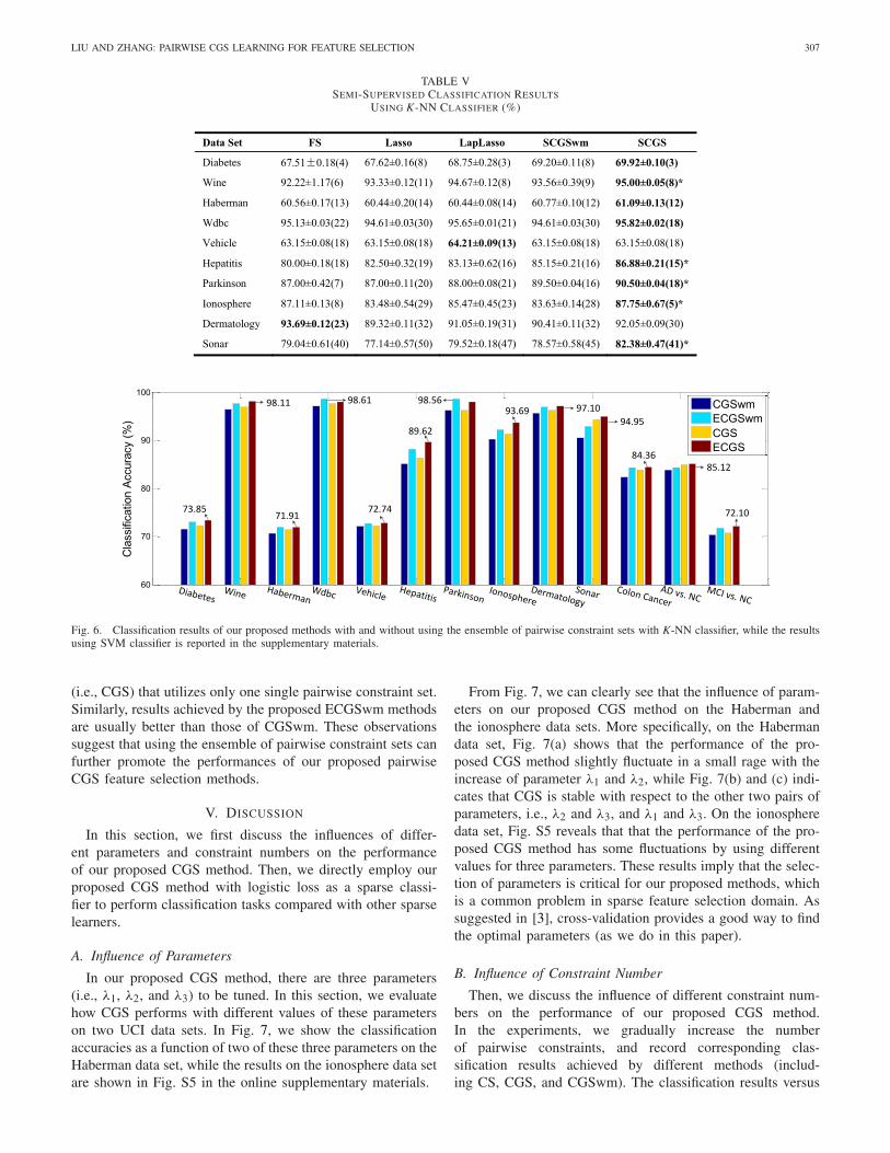
TABLE VSEMI-SUPERVISED CLASSIFICATION RESULTS

USING K-NN CLASSIFIER (%)

Fig. 6. Classification results of our proposed methods with and without using the ensemble of pairwise constraint sets with K-NN classifier, while the resultsusing SVM classifier is reported in the supplementary materials.

(i.e., CGS) that utilizes only one single pairwise constraint set.Similarly, results achieved by the proposed ECGSwm methodsare usually better than those of CGSwm. These observationssuggest that using the ensemble of pairwise constraint sets canfurther promote the performances of our proposed pairwiseCGS feature selection methods.

V. DISCUSSION

In this section, we first discuss the influences of differ-ent parameters and constraint numbers on the performanceof our proposed CGS method. Then, we directly employ ourproposed CGS method with logistic loss as a sparse classi-fier to perform classification tasks compared with other sparselearners.

A. Influence of Parameters

In our proposed CGS method, there are three parameters(i.e., λ1, λ2, and λ3) to be tuned. In this section, we evaluatehow CGS performs with different values of these parameterson two UCI data sets. In Fig. 7, we show the classificationaccuracies as a function of two of these three parameters on theHaberman data set, while the results on the ionosphere data setare shown in Fig. S5 in the online supplementary materials.

From Fig. 7, we can clearly see that the influence of param-eters on our proposed CGS method on the Haberman andthe ionosphere data sets. More specifically, on the Habermandata set, Fig. 7(a) shows that the performance of the pro-posed CGS method slightly fluctuate in a small rage with theincrease of parameter λ1 and λ2, while Fig. 7(b) and (c) indi-cates that CGS is stable with respect to the other two pairs ofparameters, i.e., λ2 and λ3, and λ1 and λ3. On the ionospheredata set, Fig. S5 reveals that that the performance of the pro-posed CGS method has some fluctuations by using differentvalues for three parameters. These results imply that the selec-tion of parameters is critical for our proposed methods, whichis a common problem in sparse feature selection domain. Assuggested in [3], cross-validation provides a good way to findthe optimal parameters (as we do in this paper).

B. Influence of Constraint Number

Then, we discuss the influence of different constraint num-bers on the performance of our proposed CGS method.In the experiments, we gradually increase the numberof pairwise constraints, and record corresponding clas-sification results achieved by different methods (includ-ing CS, CGS, and CGSwm). The classification results versus


Fig. 7. Classification accuracies versus parameters λ1, λ2, and λ3 on the Haberman data set. (a) Fixed λ1. (b) Fixed λ2. (c) Fixed λ3. Note that in (a)–(c),when two parameters vary, another is fixed as 0.001.

Fig. 8. Classification results versus the number of pairwise constraintsachieved by different methods on (a) Haberman and (b) ionosphere data sets.

number of pairwise constraints using K-NN classifier onHaberman and ionosphere data sets are given in Fig. 8, andthe results on the other four UCI data sets (i.e., hepatitis,sonar, wine, and Parkinson) are shown in Fig. S6 in the onlinesupplementary materials.

As shown in Fig. 8(a), on the Haberman data set, the over-all performances of the proposed CGS and CGSwm methodsgradually become better with the increase of constraint num-ber in a large scale. When the number of constraint is largerthan 360, the performance of CGS has some fluctuations.On the ionosphere data set, from Fig. 8(b), we can see thaton the whole the performances of CGS gradually increasewhen the constraint number increases. These results imply thatadding more side information (i.e., pairwise constraints) helpimprove the classification results. On the other hand, despite ofdifferent pairwise constraint numbers, CGS consistently out-performs CS, while in most cases CGSwm performs betterthan CS.

C. Comparison With Sparse Classifiers

As shown in (14), the proposed CGS model can beused as a sparse classifier by using a logistic loss func-tion. In this section, we employ CGS with logistic loss asa sparse classifier, and compare it with L1 logistic regressionmodel (L1_log) and Laplacian regularized L1 logistic regres-sion model (LapL1_log). We denote our proposed methodwith logistic loss function as CGS_log and CGSwm_log,respectively. In Table VI, we report the classification results onseven two-class UCI data sets achieved by four sparse learners.

TABLE VIRESULTS USING DIFFERENT SPARSE CLASSIFIERS (%)

From Table VI, we can see that our proposed CGS_logmethod significantly outperforms L1_log and LapL1_log,while the proposed CGSwm_log performs better than L1_logand LapL1_log on those seven UCI data sets. On the otherhand, one can find another interesting observation fromTables IV, VI, and SI. That is, our proposed CGS_logmethod generally outperforms CGS with both K-NN and SVMclassifiers, and the proposed CGSwm_log usually performsbetter than CGSwm with both K-NN and SVM classifiers.The underlying reason could be that the selected featuresin CGS_log and CGSwm_log are very suitable for theircorresponding classifiers, because both selected features andcorresponding classifiers are learned from a same objectivefunction. It indicates that our proposed model can not only beused for performing feature selection, but also be effective toperform classification tasks as sparse learners.

VI. CONCLUSION

In this paper, we propose a pairwise CGS learning methodfor feature selection, where pairwise constraints are used asdiscriminative regularization terms that concentrate on thelocal discriminative structure of data by using the underly-ing supervised information conveyed by the must-link and thecannot-link constraints. Furthermore, we extend our proposedCGS method into a SCGS method and an ECGS method.Experimental results on a number of data sets validate theefficacy of our proposed methods.

In this paper, the number of selected features mainlydepends on the parameter of L1-norm regularization, which is


very limited. To select an optimal feature subset with a fixedsize based on the needs of specific tasks seems to be moreappealing, which is one of our future works. In addition, weplan to adapt our proposed pairwise CGS learning methods tomultimodality learning problems.

ACKNOWLEDGMENT

The authors would like to thank the editor and the anony-mous reviewers for their constructive comments and contribu-tions for the improvement of this paper.

REFERENCES

[1] N. Kwak and C. H. Choi, “Input feature selection by mutual informa-tion based on Parzen window,” IEEE Trans. Pattern Anal. Mach. Intell.,vol. 24, no. 12, pp. 1667–1671, Dec. 2002.

[2] H. Peng, F. Long, and C. Ding, “Feature selection based onmutual information: Criteria of max-dependency, max-relevance andmin-redundancy,” IEEE Trans. Pattern Anal. Mach. Intell., vol. 27, no. 8,pp. 1226–1238, Aug. 2005.

[3] T. Hastie, R. Tibshirani, and J. J. H. Friedman, The Elements ofStatistical Learning. New York, NY, USA: Springer, 2001.

[4] A. R. Webb, Statistical Pattern Recognition. London, U.K.: Arnold,1999.

[5] S. Li and D. Wei, “Extremely high-dimensional feature selection via fea-ture generating samplings,” IEEE Trans. Cybern., vol. 44, no. 6,pp. 737–747, Jun. 2014.

[6] H. Richang et al., “Image annotation by multiple-instance learning withdiscriminative feature mapping and selection,” IEEE Trans. Cybern.,vol. 44, no. 5, pp. 669–680, May 2014.

[7] D. Ren, C. Fei, P. Taoxin, N. Snooke, and S. Qiang, “Feature selectioninspired classifier ensemble reduction,” IEEE Trans. Cybern., vol. 44,no. 8, pp. 1259–1268, Aug. 2014.

[8] A. K. Jain, R. P. W. Duin, and J. Mao, “Statistical pattern recognition:A review,” IEEE Trans. Pattern Anal. Mach. Intell., vol. 22, no. 1,pp. 4–37, Jan. 2000.

[9] I. Cohen, F. G. Cozman, N. Sebe, M. C. Cirelo, and T. S. Huang,“Semisupervised learning of classifiers: Theory, algorithms, and theirapplication to human-computer interaction,” IEEE Trans. Pattern Anal.Mach. Intell., vol. 26, no. 12, pp. 1553–1566, Dec. 2004.

[10] O. Chapelle, B. Schölkopf, and A. Zien, Semi-Supervised Learning,vol. 2. Cambridge, MA, USA: MIT Press, 2006.

[11] H. Chenping, N. Feiping, L. Xuelong, Y. Dongyun, and W. Yi, “Jointembedding learning and sparse regression: A framework for unsu-pervised feature selection,” IEEE Trans. Cybern., vol. 44, no. 6,pp. 793–804, Jun. 2014.

[12] J. Yu, R. Rui, and B. Chen, “Exploiting click constraints and multi-viewfeatures for image re-ranking,” IEEE Trans. Multimedia, vol. 16, no. 1,pp. 159–168, Jan. 2014.

[13] W. Liu, H. Zhang, D. Tao, Y. Wang, and K. Lu, “Large-scale paralleledsparse principal component analysis,” Multimedia Tools Appl., pp. 1–13,2013.

[14] J. Yu, D. Liu, D. Tao, and H. S. Seah, “Complex object correspon-dence construction in two-dimensional animation,” IEEE Trans. ImageProcess., vol. 20, no. 11, pp. 3257–3269, Nov. 2011.

[15] M. S. Baghshah and S. B. Shouraki, “Semi-supervised metric learn-ing using pairwise constraints,” in Proc. Int. Joint Conf. Artif. Intell.,Pasadena, CA, USA, 2009, pp. 1217–1222.

[16] W. Liu, S. Ma, D. Tao, J. Liu, and P. Liu, “Semi-supervised sparsemetric learning using alternating linearization optimization,” in Proc.16th ACM SIGKDD Int. Conf. Knowl. Disc. Data Min., Washington,DC, USA, 2010, pp. 1139–1148.

[17] F. Wang, “Semisupervised metric learning by maximizing constraintmargin,” IEEE Trans. Syst., Man, Cybern. B, Cybern., vol. 41, no. 4,pp. 931–939, Aug. 2011.

[18] A. Mignon and F. Jurie, “PCCA: A new approach for distance learningfrom sparse pairwise constraints,” in Proc. IEEE Conf. Comput. Vis.Pattern Recognit., Providence, RI, USA, 2012, pp. 2666–2672.

[19] I. Davidson and S. Basu, “A survey of clustering with instance levelconstraints,” ACM Trans. Knowl. Disc. Data, vol. w, no. x, pp. 1–41,2007.

[20] H. Zeng and Y.-M. Cheung, “Semi-supervised maximum margin cluster-ing with pairwise constraints,” IEEE Trans. Knowl. Data Eng., vol. 24,no. 5, pp. 926–939, May 2012.

[21] W. Zhao, Q. He, H. Ma, and Z. Shi, “Effective semi-supervised doc-ument clustering via active learning with instance-level constraints,”Knowl. Inf. Syst., vol. 30, no. 3, pp. 569–587, 2012.

[22] S. Ding, H. Jia, L. Zhang, and F. Jin, “Research of semi-supervised spec-tral clustering algorithm based on pairwise constraints,” Neural Comput.Appl., vol. 24, no. 1, pp. 211–219, 2014.

[23] F. Nie, D. Xu, I. W.-H. Tsang, and C. Zhang, “Flexible manifoldembedding: A framework for semi-supervised and unsuperviseddimension reduction,” IEEE Trans. Image Process., vol. 19, no. 7,pp. 1921–1932, Jul. 2010.

[24] C. Xu, D. Tao, C. Xu, and Y. Rui, “Large-margin weakly superviseddimensionality reduction,” in Proc. Int. Conf. Mach. Learn., Beijing,China, 2014, pp. 865–873.

[25] D. Zhang, S. Chen, and Z.-H. Zhou, “Constraint score: A new fil-ter method for feature selection with pairwise constraints,” PatternRecognit., vol. 41, no. 5, pp. 1440–1451, 2008.

[26] D. Sun and D. Zhang, “Bagging constraint score for feature selec-tion with pairwise constraints,” Pattern Recognit., vol. 43, no. 6,pp. 2106–2118, 2010.

[27] M. Kalakech, P. Biela, L. Macaire, and D. Hamad, “Constraint scoresfor semi-supervised feature selection: A comparative study,” PatternRecognit. Lett., vol. 32, no. 5, pp. 656–665, 2011.

[28] M. Liu and D. Zhang, “Sparsity score: A novel graph-preserving featureselection method,” Int. J. Pattern Recognit. Artif. Intell., vol. 28, no. 4,2014, Art. ID 1450009.

[29] R. Tibshirani, “Regression shrinkage and selection via the lasso,” J. Roy.Stat. Soc. B, Met., vol. 58, no. 1, pp. 267–288, 1996.

[30] R. Tibshirani, M. Saunders, S. Rosset, J. Zhu, and K. Knight, “Sparsityand smoothness via the fused lasso,” J. Roy. Statist. Soc. B, Stat. Met.,vol. 67, no. 1, pp. 91–108, 2005.

[31] L. Meier, S. Van De Geer, and P. Bühlmann, “The group lasso for logisticregression,” J. Roy. Statist. Soc. B, Stat. Met., vol. 70, no. 1, pp. 53–71,2008.

[32] D. Zhang, Y. Wang, L. Zhou, H. Yuan, and D. Shen, “Multimodalclassification of Alzheimer’s disease and mild cognitive impairment,”Neuroimage, vol. 55, no. 3, pp. 856–867, 2011.

[33] J. Wright, A. Y. Yang, A. Ganesh, S. S. Sastry, and Y. Ma, “Robust facerecognition via sparse representation,” IEEE Trans. Pattern Anal. Mach.Intell., vol. 31, no. 2, pp. 210–227, Feb. 2009.

[34] Y. Xie et al., “Discriminative object tracking via sparse representationand online dictionary learning,” IEEE Trans. Cybern., vol. 44, no. 4,pp. 539–553, Apr. 2014.

[35] C. M. Bishop, Neural Networks for Pattern Recognition. Oxford, U.K.:Oxford Univ. Press, 1995.

[36] X. He, D. Cai, and P. Niyogi, “Laplacian score for feature selection,”in Proc. Adv. Neural Inf. Process. Syst., Whistler, BC, Canada, 2005,pp. 507–514.

[37] M. Belkin and P. Niyogi, “Laplacian eigenmaps for dimensionalityreduction and data representation,” Neural Comput., vol. 15, no. 6,pp. 1373–1396, 2003.

[38] P. K. Mallapragada, R. Jin, and A. K. Jain, “Online visual vocabularypruning using pairwise constraints,” in Proc. IEEE Conf. Comput. Vis.Pattern Recognit., San Francisco, CA, USA, 2010, pp. 3073–3080.

[39] H. Li, X. Wang, J. Tang, and C. Zhao, “Combining global andlocal matching of multiple features for precise item image retrieval,”Multimedia Syst., vol. 19, no. 1, pp. 37–49, 2013.

[40] H. Zou and T. Hastie, “Regularization and variable selection via theelastic net,” J. Roy. Stat. Soc. B, Stat. Met., vol. 67, no. 2, pp. 301–320,2005.

[41] N. Kwak, “Principal component analysis based on L1-normmaximization,” IEEE Trans. Pattern Anal. Mach. Intell., vol. 30,no. 9, pp. 1672–1680, Sep. 2008.

[42] W. Liu and D. Tao, “Multiview Hessian regularization for imageannotation,” IEEE Trans. Image Process., vol. 22, no. 7, pp. 2676–2687,Jul. 2013.

[43] W. Liu, D. Tao, J. Cheng, and Y. Tang, “Multiview hessian discriminativesparse coding for image annotation,” Comput. Vis. Image Understand.,vol. 118, pp. 50–60, Jan. 2014.

[44] H. Xue and S. Chen, “Discriminality-driven regularization frameworkfor indefinite kernel machine,” Neurocomputing, vol. 133, pp. 209–221,Jun. 2014.

[45] H. Xue, S. Chen, and Q. Yang, “Discriminatively regularizedleast-squares classification,” Pattern Recognit., vol. 42, no. 1,pp. 93–104, 2009.


[46] F. R. Chung, Spectral Graph Theory. Providence, RI, USA: Amer. Math.Soc., 1997.

[47] C. Li and H. Li, “Network-constrained regularization and variable selec-tion for analysis of genomic data,” Bioinformatics, vol. 24, no. 9,pp. 1175–1182, 2008.

[48] X. Chen, W. Pan, J. T. Kwok, and J. G. Carbonell, “Accelerated gradientmethod for multitask sparse learning problem,” in Proc. IEEE Int. Conf.Data Min., Miami, FL, USA, 2009, pp. 746–751.

[49] A. Beck and M. Teboulle, “A fast iterative shrinkage-thresholding algo-rithm for linear inverse problems,” SIAM J. Imag. Sci., vol. 2, no. 1,pp. 183–202, 2009.

[50] J. J. E. Dennis and R. B. Schnabel, Numerical Methods forUnconstrained Optimization and Nonlinear Equations. Philadelphia, PA,USA: SIAM, 1983.

[51] J. Liu and J. Ye, “Efficient L1/Lq norm regularization,” Dept. Comput.Sci. Eng., Arizona State Univ., Tucson, AZ, USA, Tech. Rep., 2009.

[52] A. Frank and A. Asuncion, UCI Machine Learning Repository, SchoolInf. Comput. Sci., Univ. California, Irvine, CA, USA, 2007.

[53] K. L. Wagstaff, Value, Cost, and Sharing: Open Issues in ConstrainedClustering. New York, NY, USA: Springer, 2007.

[54] T. G. Dietterichl, “Ensemble learning,” in The Handbook of BrainTheory and Neural Networks. Cambridge, MA, USA: MIT Press, 2002,pp. 405–408.

[55] M. Liu, D. Zhang, and D. Shen, View-Centralized Multi-AtlasClassification for Alzheimer’s Disease Diagnosis. New York, NY, USA:Human Brain Map., 2015.

[56] C. Xu, D. Tao, and C. Xu, “A survey on multi-view learning,” NeuralComput. Appl., vol. 23, no. 7–8, pp. 2031–2038, 2013.

[57] U. Alon et al., “Broad patterns of gene expression revealed by clusteringanalysis of tumor and normal colon tissues probed by oligonucleotidearrays,” Proc. Nat. Acad. Sci. USA, vol. 96, pp. 6745–6750, Jun. 1999.

[58] A. Farhadi, I. Endres, and D. Hoiem, “Attribute-centric recognition forcross-category generalization,” in Proc. IEEE Conf. Comput. Vis. PatternRecognit., San Francisco, CA, USA, 2010, pp. 2352–2359.

[59] O. Russakovsky and L. Fei-Fei, “Attribute learning in large-scaledatasets,” in Proc. Workshop Parts Attributes Eur. Conf. Comput. Vis.,Crete, Greece, 2010, pp. 10–11.

[60] H. Fei, B. Quanz, and J. Huan, “Regularization and feature selection fornetworked features,” in Proc. Int. Conf. Inf. Knowl. Manage., Toronto,ON, Canada, 2010, pp. 1893–1896.

[61] C.-C. Chang and C.-J. Lin, “LIBSVM: A library for support vectormachines,” ACM Trans. Intell. Syst. Technol., vol. 2, no. 3, p. 27, 2011.

Mingxia Liu received the B.S. and M.S. degreesfrom Shandong Normal University, Shandong,China, in 2003 and 2006, respectively, and the Ph.D.degree from Nanjing University of Aeronautics andAstronautics, Nanjing, China, in 2015.

Her current research interests include neuroimag-ing analysis, machine learning, pattern recognition,and data mining.

Daoqiang Zhang received the B.S. andPh.D. degrees in computer science fromthe Nanjing University of Aeronautics andAstronautics (NUAA), Nanjing, China, in 1999 and2004, respectively.

In 2004, he joined the Department of ComputerScience and Engineering, NUAA, as a Lecturer,where he is currently a Professor. His currentresearch interests include machine learning, patternrecognition, data mining, and medical imageanalysis. He has published over 100 scientific

articles in refereed international journals such as the IEEE TRANSACTIONS

ON PATTERN ANALYSIS AND MACHINE INTELLIGENCE, Neuroimage,Human Brain Mapping, and conference proceedings such as InternationalJoint Conferences on Artificial Intelligence, IEEE International Conferenceon Data Mining, and International Conference on Medical Image Computingand Computer Assisted Interventions.

Dr. Zhang is a member of the Machine Learning Society of the ChineseAssociation of Artificial Intelligence and the Artificial Intelligence andPattern Recognition Society of the China Computer Federation.

Documents

298 IEEE TRANSACTIONS ON CYBERNETICS, VOL. 46, NO. 1