IEEE TRANSACTIONS ON CYBERNETICS, VOL. 99 , NO. PP, IN

arX

iv:1

311.

6107

v3 [

cs.S

Y]

11 M

ay 2

014

IEEE TRANSACTIONS ON CYBERNETICS, VOL. 99 , NO. PP, IN PRESS,2014 1

Off-policy Reinforcement Learning forH∞ ControlDesign

Biao Luo, Huai-Ning Wu and Tingwen Huang

Abstract—The H∞ control design problem is considered fornonlinear systems with unknown internal system model. It isknown that the nonlinear H∞ control problem can be trans-formed into solving the so-called Hamilton-Jacobi-Isaacs(HJI)equation, which is a nonlinear partial differential equation that isgenerally impossible to be solved analytically. Even worse, model-based approaches cannot be used for approximately solvingHJI equation, when the accurate system model is unavailableor costly to obtain in practice. To overcome these difficulties,an off-policy reinforcement leaning (RL) method is introducedto learn the solution of HJI equation from real system datainstead of mathematical system model, and its convergence isproved. In the off-policy RL method, the system data can begenerated with arbitrary policies rather than the evaluatingpolicy, which is extremely important and promising for practicalsystems. For implementation purpose, a neural network (NN)based actor-critic structure is employed and a least-square NNweight update algorithm is derived based on the method ofweighted residuals. Finally, the developed NN-based off-policyRL method is tested on a linear F16 aircraft plant, and furtherapplied to a rotational/translational actuator system.

Index Terms—H∞ control design; Reinforcement learning;Off-policy learning; Neural Network; Hamilton-Jacobi-Is aacsequation.

I. I NTRODUCTION

REINFORCEMENT learning (RL) is a machine learn-ing technique that has been widely studied from the

computational intelligence and machine learning scope in theartificial intelligence community [1]–[4]. RL technique refersto an actor or agent that interacts with its environment andaims to learn the optimal actions, or control policies, by

Manuscript received November 24, 2013; revised March 28, 2014 and April2, 2014; accepted April 18, 2014. This work was supported in part by theNational Basic Research Program of China under 973 Program of Grant2012CB720003, in part by the National Natural Science Foundation of Chinaunder Grant 61121003, and in part by the General Research Fund project fromScience and Technology on Aircraft Control Laboratory of Beihang Universityunder Grant 9140C480301130C48001. This publication was also made possi-ble by NPRP grant # NPRP 4-1162-1-181 from the Qatar NationalResearchFund (a member of Qatar Foundation). The statements made herein are solelythe responsibility of the authors. This paper was recommended by AssociateEditor H. M. Schwartz.

Biao Luo is with the Science and Technology on Aircraft Control Labo-ratory, Beihang University (Beijing University of Aeronautics and Astronau-tics), Beijing 100191, P. R. China. He is also with State Key Laboratoryof Management and Control for Complex Systems, Institute ofAutoma-tion, Chinese Academy of Sciences, Beijing 100190, P. R. China (E-mail:[email protected]).

Huai-Ning Wu is with the Science and Technology on Aircraft ControlLaboratory, Beihang University (Beijing University of Aeronautics and As-tronautics), Beijing 100191, P. R. China (E-mail:[email protected]).

Tingwen Huang is with the Texas A& M University at Qatar, PO Box23874, Doha, Qatar (E-mail: [email protected]).

Digital Object Identifier 10.1109/TCYB.2014.2319577

observing their responses from the environment. In [2], Suttonand Barto suggested a definition of RL method, i.e., anymethod that is well suited for solving RL problem can beregarded as a RL method, where the RL problem is definedin terms of optimal control of Markov decision processes.This obviously established the relationship between the RLmethod and control community. Moreover, RL methods havethe ability to find an optimal control policy from unknownenvironment, which makes RL a promising method for controldesign of real systems.

In the past few years, many RL approaches [5]–[23] havebeen introduced for solving the optimal control problems.Especially, some extremely important results were reportedby using RL for solving the optimal control problem ofdiscrete-time systems [7], [10], [14], [17], [18], [22]. Suchas, Liu and Wei suggested a finite-approximation-error basediterative adaptive dynamic programming approach [17], anda novel policy iteration (PI) method [22] for discrete-timenonlinear systems. For continuous-time systems, Murray etal. [5] presented two PI algorithms that avoid the necessityofknowing the internal system dynamics. Vrabie et al. [8], [9],[13] introduced the thought of PI and proposed an importantframework of integral reinforcement learning (IRL). Modareset al. [21] developed an experience replay based IRL algorithmfor nonlinear partially unknown constrained-input systems.In [19], an online neural network (NN) based decentralizedcontrol strategy was developed for stabilizing a class ofcontinuous-time nonlinear interconnected large-scale systems.In addition, it worth mentioning that the thought of RLmethods have also been introduced to solve the optimal controlproblem of partial differential equation systems [6], [12], [15],[16], [23]. However, for most of practical real systems, theexistence of external disturbances is usually unavoidable.

To reduce the effects of disturbance, robust controller isrequired for disturbance rejection. One effective solution is theH∞ control method, which achieves disturbance attenuationin theL2-gain setting [24]–[26], that is, to design a controllersuch that the ratio of the objective output energy to thedisturbance energy is less than a prescribed level. Over thepast few decades, a large number of theoretical results onnonlinearH∞ control have been reported [27]–[29], where theH∞ control problem can be transformed into how to solve theso-called Hamilton-Jacobi-Isaacs (HJI) equation. However, theHJI equation is a nonlinear partial differential equation (PDE),which is difficult or impossible to solve, and may not haveglobal analytic solutions even in simple cases.

Thus, some works have been reported to solve the HJI equa-tion approximately [27], [30]–[35]. In [27], it was shown that

http://arxiv.org/abs/1311.6107v3


there exists a sequence of policy iterations on the control inputsuch that the HJI equation is successively approximated witha sequence of Hamilton-Jacobi-Bellman (HJB)-like equations.Then, the methods for solving HJB equation can be extendedfor the HJI equation. In [36], the HJB equation was succes-sively approximated by a sequence of linear PDEs, which weresolved with Galerkin approximation in [30], [37], [38]. In[39], the successive approximation method was extended tosolve the discrete-time HJI equation. Similar to [30], a policyiteration scheme was developed in [31] for the constrainedinput system. For implementation purpose of this scheme,a neuro-dynamic programming approach was introduced in[40] and an online adaptive method was given in [41]. Thisapproach suits for the case that the saddle point exists, thusa situation that the smooth saddle point does not exist wasconsidered in [42]. In [32], a synchronous policy iterationmethod was developed, which is the extension of the work[43]. To improve the efficiency for computing the solutionof HJI equation, Luo and Wu [44] proposed a computation-ally efficient simultaneous policy update algorithm (SPUA).In addition, in [45] the solution of the HJI equation wasapproximated by the Taylor series expansion, and an efficientalgorithm was furnished to generate the coefficients of the Tay-lor series. It is observed that most of these methods [27], [30]–[33], [35], [40], [44], [45] are model-based, where the fullsystem model is required. However, the accurate system modelis usually unavailable or costly to obtain for many practicalsystems. Thus, some RL approaches have been proposed forH∞ control design of linear systems [46], [47] and nonlinearsystems [48] with unknown internal system model. But thesemethods are on-policy learning approaches [32], [41], [46]–[49], where the cost function should be evaluated by usingsystem data generated with policies being evaluated. It is foundthat there are several drawbacks (to be discussed in SectionIII) to apply the on-policy learning to solve realH∞ controlproblem.

To overcome this problem, this paper introduces an off-policy RL method to solve the nonlinear continuous-timeH∞

control problem with unknown internal system model. The restof the paper is rearranged as follows. Sections II and III presentthe problem description and the motivation. The off-policylearning methods for nonlinear systems and linear systems aredeveloped in IV and V respectively. The simulation studiesare conducted in Section VI and a brief conclusion is givenin Section VII.

Notations: R,Rn and Rn×m are the set of real numbers,

the n-dimensional Euclidean space and the set of all realmatrices, respectively.‖ · ‖ denotes the vector norm or matrixnorm in R

n or Rn×m , respectively. The superscriptT is

used for the transpose andI denotes the identify matrixof appropriate dimension.▽ , ∂/∂x denotes a gradientoperator notation. For a symmetric matrixM,M > (>)0means that it is a positive (semi-positive) definite matrix.‖v‖2M , vTMv for some real vectorv and symmetric matrixM > (>)0 with appropriate dimensions.C1(X ) is functionspace onX with first derivatives are continuous.L2[0,∞)is a Banach space, for∀w(t) ∈ L2[0,∞),

∫∞

0 ‖w(t)‖2dt <

∞. Let X ,U and W be compact sets, denoteD ,

{(x, u, w)|x ∈ X , u ∈ U , w ∈ W}. For column vectorfunctions s1(x, u, w) and s2(x, u, w) , where (x, u, w) ∈D define inner product〈s1(x, u, w), s2(x, u, w)〉D ,∫DsT1 (x, u, w)s2(x, u, w)d(x, u, w) and norm‖s1(x, u, w)‖D

,(∫

DsT1 (x, u, w)s1(x, u, w)d(x, u, w)

)1/2. Hm,p(X ) is a

Sobolev space that consists of functions in spaceLp(X ) suchthat their derivatives of order at leastm are also inLp(X ).

II. PROBLEM DESCRIPTION

Let us consider the following affine nonlinear continuous-time dynamical system:

x(t) = f(x(t)) + g(x(t))u(t) + k(x(t))w(t) (1)

z(t) = h(x) (2)

where[x1 ... xn]T ∈ X ⊂ R

n is the state,u = [u1 ... um]T ∈U ⊂ R

m is the control input andu(t) ∈ L2[0,∞), w =[w1 ... wq]

T ∈ W ⊂ Rq is the external disturbance andw(t) ∈

L2[0,∞), z = [z1 ... zp]T ∈ R

p is the objective output.f(x)is Lipschitz continuous on a setX that contains the origin,f(0) = 0. f(x) represents the internal system model which isassumed to beunknownin this paper.g(x), k(x) andh(x) areknown continuous vector or matrix functions of appropriatedimensions.

The H∞ control problem under consideration is to find astate feedback control lawu(x) such that the system (1) isclosed-loop asymptotically stable, and hasL2-gain less thanor equal toγ , that is,

∫ ∞

0

(‖z(t)‖2 + ‖u(t)‖2R

)dt ≤ γ2

∫ ∞

0

‖w(t)‖2dt (3)

for all w(t) ∈ L2[0,∞), R > 0 andγ > 0 is some prescribedlevel of disturbance attenuation. From [27], this problem canbe transformed to solve the so-called HJI equation, which issummarized in Lemma 1.

Lemma 1. Assume the system(1) and (2) is zero-stateobservable. Forγ > 0 , suppose there exists a solutionV ∗(x)to the HJI equation

[∇V ∗(x)]T f(x) + hT (x)h(x)

− 1

4[∇V ∗(x)]T g(x)R−1gT (x)∇V ∗(x)

+1

4γ2[∇V ∗(x)]T k(x)kT (x)∇V ∗(x) = 0. (4)

whereV ∗(x) ∈ C1(X ), V ∗(x) > 0 andV ∗(0) = 0. Then, theclosed-loop system with the state feedback control

u(t) = u∗(x(t)) = −1

2R−1gT (x)∇V ∗(x) (5)

hasL2-gain less than or equal toγ, and the closed-loop sys-tem(1), (2) and (5) (whenw(t) ≡ 0 ) is locally asymptoticallystable.�

III. M OTIVATION FROM INVESTIGATION OF RELATED

WORK

From Lemma 1, it is noted that theH∞ control (5) relies onthe solution of the HJI equation (4). Therefore, a model-based


iterative method was proposed in [30], where the HJI equationis successively approximated by a sequence of linear PDEs:

[∇V (i,j+1)]T (f + gu(i) + kw(i,j)) + hTh+ ‖u(i)‖2R−γ2‖w(i,j)‖2 = 0 (6)

and then update control and disturbance policies with

w(i,j+1) ,1

2γ−2kT∇V (i,j+1) (7)

u(i+1) , −1

2R−1gT∇V (i+1) (8)

with V (i+1) , limj→∞

V (i,j). From [27], [30], it was indicated

that theV (i,j) can converge to the solution of the HJI equation,i.e., lim

i,j→∞V (i,j) = V ∗.

Remark 1. Note that the key point of the iterative scheme(6)-(8) depends on the solution of the linear PDE (6). Thus,several related methods were developed, such as, Galerkinapproximation [30], synchronous policy iteration [32], neuro-dynamic programming approach [31], [40] and online adap-tive control method [41] for constrained input systems, andGalerkin approximation method for discrete-time systems [39].Obviously, the iteration (6)-(8) will generate two iterativeloops since the control and disturbance policies are updated atthe different iterative steps, i.e., the inner loop for updatingdisturbance policyw with index j, and the outer iterativeloop for updating control policyu with index i. The outerloop will not be activated until the inner loop is convergent,which results in low efficiency. Therefore, Luo and Wu [44]proposed a simultaneous policy update algorithm (SPUA),where the control and disturbance policies are updated at thesame iterative step, and thus only one iterative loop is required.It worth noting that the word “simultaneous” in [44] andthe word “synchronous/simultaneous” in [32], [41] representdifferent meanings. The former emphasizes the same “iterativestep, while the latter emphasizes the same “time instant”. Inother words, the SPUA in [44] updates control and disturbancepolicies at the “same” iterative step, while the algorithmsin [32], [41] update control and disturbance policies at the“different” iterative steps.�

The procedure of model-based SPUA is given in Algorithm1.

Algorithm 1. Model-based SPUA.

◮ Step 1:Give an initial functionV (0) ∈ V0 (V0 ⊂ V isdetermined by Lemma 5 in [44]. Leti = 0 ;

◮ Step 2:Update the control and disturbance policies with

u(i) , −1

2R−1gT∇V (i) (9)

w(i) ,1

2γ−2kT∇V (i) (10)

◮ Step 3:Solve the following linear PDE forV (i+1)(x) :

[∇V (i+1)]T (f + gu(i) + kw(i)) + hTh+ ‖u(i)‖2R−γ2‖w(i)‖2 = 0; (11)

where V (i+1)(x) ∈ C1(X ), V (i+1)(x) > 0 andV (i+1)(0) = 0.

◮ Step 4:Let i = i+1, go back to Step 2 and continue.�

It worth noting that Algorithm 1 is an infinite iterativeprocedure, which is used for theoretical analysis rather thanfor implementation purpose. That is to say, Algorithm 1will converge to the solution of the HJI equation (4) whenthe iteration goes to infinity. By constructing a fixed pointequation, the convergence of Algorithm 1 is established in [44]by proving that it is essentially a Newtons iteration methodfor finding the fixed point. With the increase of indexi,the sequenceV (i) obtained by the SPUA with equations (9)-(11) can converge to the solution of HJI equation (4), i.e.,limi→∞

V (i) = V ∗.

Remark 2. It is necessary to explain the rationale of usingequations (9) and (10) for control and disturbance policiesupdate. TheH∞ control problem (1)-(3) can be viewedas a two-players zero-sum differential game problem [26],[32]–[34], [40], [41], [47]. The game problem is a minimaxproblem, where the control policyu acts as the minimizingplayer and the disturbance policyw is the maximizing player.The game problem aims at finding the saddle point(u∗, w∗),where u∗ is given by expression (5) andw∗ is given byw∗(x) , 1

2γ−2kT (x)∇V ∗(x). Correspondingly, for theH∞

control problem (1)-(3),u∗ and w∗ are the associatedH∞

control policy and the worst disturbance signal [26], [31],[32], [34], [40], [47], respectively. Thus, it is reasonable usingexpressions (9) and (10) (that are consistent withu∗ andw∗

in form) for control and disturbance policies update. Similarcontrol and disturbance policy update method could be foundin references [27], [30], [31], [34], [40], [41].�

Observe that both iterative equations (6) and (11) requirethe full system model. For theH∞ control problem that theinternal system dynamicf(x) is unknown, data based methods[47], [48] were suggested to solve the HJI equation online.However, most of related existing online methods are on-policy learning approaches [32], [41], [47]–[49]. From thedefinition of on-policy learning [2], the cost function should beevaluated with the data generated from the evaluating policies.For example,V (i,j+1) in equation (6) is the cost function ofthe policiesw(i,j) andu(i), which means thatV (i,j+1) shouldbe evaluated with system data by using evaluating policiesw(i,j) and u(i). It is observed that these on-policy learningapproaches for solving theH∞ control problem have severaldrawbacks:

• 1) For real implementation of on-policy learning methods[32], [41], [48], [49], the approximate evaluating controland disturbance policies (rather than the actual policies)are used to generate data for learning their cost function.In other words, the on-policy learning methods using the“inaccurate” data to learn their cost function, which willincrease the accumulated error. For example, to learn thecost functionV (i,j+1) in equation (6), some approximatepolicies w(i,j) and u(i) (rather than its actual policiesw(i,j) and u(i), which are usually unknown because of


estimate error) are employed to generate data;• 2) The evaluating control and disturbance policies are

required to generate data for on-policy learning, thusdisturbance signal should be adjustable, which is usuallyimpractical for most of real systems;

• 3) It is known [2], [50] that the issue of “exploration”is extremely important in RL for learning the optimalcontrol policy, and the lack of exploration during thelearning process may lead to divergency. Nevertheless,for on-policy learning, exploration is restricted becauseonly the evaluating policies can be used to generate data.From the literature investigation, it is found that the“exploration” issue is rarely discussed in existing workthat using RL techniques for control design;

• 4) The implementation structure is complicated, such asin [32], [41], three NNs are required for approximatingcost function, control and disturbance policies, respec-tively;

• 5) Most of existing approaches [32], [41], [47]–[49]are implemented online, thus they are difficult forreal-time control because the learning process is oftentime-consuming. Furthermore, online control design ap-proaches just use current data while discard past data,which implies that the measured system data is used onlyonce and thus results in low utilization efficiency.

To overcome the drawbacks mentioned above, we propose anoff-policy RL approach to solve theH∞ control problem withunknown internal system dynamicf(x).

IV. OFF-POLICY REINFORCEMENT LEARNING FORH∞

CONTROL

In this section, an off-policy RL method forH∞ controldesign is derived and its convergence is proved. Then, a NN-based critic-actor structure is developed for implementationpurpose.

A. Off-policy reinforcement learning

To derive the off-policy RL method, we rewrite the system(1) as:

x = f + gu(i) + kw(i) + g[u− u(i)] + k[w − w(i)]. (12)

for ∀u ∈ U , w ∈ W . Let V (i+1)(x) be the solution of thelinear PDE (11), then taking derivative along the state ofsystem (12) yields,

dV (i+1)(x)

dt= [∇V (i+1)]T (f + gu(i) + kw(i))

+ [∇V (i+1)]T g[u− u(i)] + [∇V (i+1)]T k[w − w(i)]. (13)

With the linear PDE (11), conducting integral on both sidesof equation (13) in time interval[t, t + ∆t] and rearrangingterms yield,∫ t+∆t

t

[∇V (i+1)(x(τ))]T g(x(τ))[u(τ) − u(i)(x(τ))]dτ

+

∫ t+∆t

t

[∇V (i+1)(x(τ))]T k(x(τ))[w(τ) − w(i)(x(τ))]dτ

+ V (i+1)(x(t)) − V (i+1)(x(t+∆t))

=

∫ t+∆t

t

(hT (x(τ))h(x(τ)) + ‖u(i)(x(τ))‖2R

−γ2‖w(i)(x(τ))‖2)dτ (14)

It is observed from the equation (14) that the cost functionV (i+1) can be learned by using arbitrary input signalsu andw, rather than the evaluating policiesu(i) and w(i). Then,replacing linear PDE (11) in Algorithm 1 with (14) results inthe off-policy RL method. To show its convergence, Theorem1 establishes the equivalence between iterative equations(11)and (14).

Theorem 1. Let V (i+1)(x) ∈ C1(X ), V (i+1)(x) > 0 andV (i+1)(0) = 0. V (i+1)(x) is the solution of equation(14) iff(if and only if ) it is the solution of the linear PDE(11), i.e.,equation(14) is equivalent to the linear PDE(11).

Proof. From the derivation of equation (14), it is concludedthat if V (i+1)(x) is the solution of the linear PDE (11), thenV (i+1)(x) also satisfies equation (14). To complete the proof,we have to show thatV (i+1)(x) is the unique solution ofequation (14). The proof is by contradiction.

Before starting the contradiction proof, we derive a simplefact. Consider

lim∆t→0

1

∆t

∫ t+∆t

t

~(τ)dτ

= lim∆t→0

1

∆t

(∫ t+∆t

0

~(τ)dτ −∫ t

0

~(τ)dτ

)

=d

dt

∫ t

0

~(τ)dτ

= ~(t). (15)

From (14), we have

dV (i+1)(x)

dt= lim

∆t→0

1

∆t

[V (i+1)(x(t +∆t))− V (i+1)(x(t))

]

= lim∆t→0

1

∆t

∫ t+∆t

t

[∇V (i+1)(x(τ))]T g(x(τ))

[u(τ)− u(i)(x(τ))]dτ

+ lim∆t→0

1

∆t

∫ t+∆t

t

[∇V (i+1)(x(τ))]T k(x(τ))

[w(τ) − w(i)(x(τ))]dτ

− lim∆t→0

1

∆t

∫ t+∆t

t

[hT (x(τ))h(x(τ)) + ‖u(i)(x(τ))‖2R

−γ2‖w(i)(x(τ))‖2]dτ. (16)

By using the fact (15), the equation (16) is rewritten as

dV (i+1)(x)

dt= [∇V (i+1)(x(t))]T g(x(t))[u(t) − u(i)(x(t))]

+ [∇V (i+1)(x(t))]T k(x(t))[w(t) − w(i)(x(t))]

−[hT (x(t))h(x(t)) + ‖u(i)(x(t))‖2R − γ2‖w(i)(x(t))‖2

].

(17)

Suppose thatW (x) ∈ C1(X ) is another solution of equation(14) with boundary conditionW (0) = 0. Thus,W (x) also


satisfies equation (17), i.e.,

dW (x)

dt= [∇W (x(t))]T g(x(t))[u(t) − u(i)(x(t))]

+ [∇W (x(t))]T k(x(t))[w(t) − w(i)(x(t))]

−[hT (x(t))h(x(t)) + ‖u(i)(x(t))‖2R − γ2‖w(i)(x(t))‖2

].

(18)

Substituting equation (18) from (17) yields,

d

dt

(V (i+1)(x)−W (x)

)

=[∇(V (i+1)(x)−W (x)

)]Tg(x)[u − u(i)(x)]

+[∇(V (i+1)(x) −W (x)

)]Tk(x)[w − w(i)(x)]. (19)

This means that equation (19) holds for∀u ∈ U , w ∈ W . Ifletting u = u(i), w = w(i), we have

d

dt

[V (i+1)(x) −W (x)

]= 0. (20)

Then, V (i+1)(x) − W (x) = c for ∀x ∈ X , where cis a real constant, andc = V (i+1)(0) − W (0) = 0 .Thus,V (i+1)(x) − W (x) = 0, i.e., W (x) = V (i+1)(x) for∀x ∈ X . This completes the proof.�

Remark 3. It follows from Theorem 1 that the solutionof equation (14) is equivalent to equation (11), and thusthe convergence of the off-policy RL is guaranteed, i.e., thesolution of the iterative equation (14) will converge to thesolution of HJI equation (4) as iteration stepi increases.Different from the equation (11) in Algorithm 1, the off-policy RL with equation (14) uses system data instead of theinternal system dynamicf(x). Hence, the off-policy RL canbe regarded as a direct learning method forH∞ control design,which avoids the identification off(x). In fact, the informationof f(x) is embedded in the measurement of system data.That is to say, the lack of knowledge aboutf(x) does nothave any impact on the off-policy RL to obtain the solutionof HJI equation (4) and theH∞ control policy. It worthpointing out that the equation (14) is similar with the formof the IRL [8], [9], which is an important framework forcontrol design of continuous-time systems. The IRL in [8],[9] is an online optimal control learning algorithm for partiallyunknown systems.�

B. Implementation based on neural network

To solve equation (14) for the unknown functionV (i+1)(x)based on system data, we develop a NN based actor-criticstructure. From the well known high-order Weierstrass ap-proximation theorem [51], a continuous function can berepresented by an infinite-dimensional linearly independentbasis function set. For real practical application, it is usuallyrequired to approximate the function in a compact set witha finite-dimensional function set. We consider the critic NNfor approximating the cost function on a compact setX .Let ϕ(x) , [ϕ1(x) ... ϕL(x)]

T be the vector of linearlyindependent activation functions for critic NN, whereϕl(x) :

X 7→ R, l = 1, ..., L, L is the number of critic NN hiddenlayer neurons. Then, the output of critic NN is given by

V (i)(x) =

L∑

l=1

θ(i)l ϕl(x) = ϕT (x)θ(i) (21)

for ∀i = 0, 1, 2, ..., whereθ(i) , [θ(i)1 ... θ

(i)L ]T is the critic

NN weight vector. It follows from (9), (10) and (21) that thedisturbance and control policies are given by:

u(i)(x) = −1

2R−1gT (x)∇ϕT (x)θ(i) (22)

w(i)(x) =1

2γ−2kT (x)∇ϕT (x)θ(i) (23)

for ∀i = 0, 1, 2, ..., and∇ϕ(x) , [∂ϕ1/∂x ... ∂ϕL/∂x]T is

the Jacobian ofϕ(x). Expressions (22) and (23) can be viewedas actor NNs for the disturbance and control policies respec-tively, where− 1

2R−1gT (x)∇ϕT (x) and 1

2γ−2kT (x)∇ϕT (x)

are the activation function vectors andθ(i) is the actor NNweight vector.

Due to estimation errors of the critic and actor NNs (21)-(23), the replacement ofV (i+1), w(i) andu(i) in the iterativeequation (14) withV (i+1), w(i) and u(i) respectively, yieldsthe following residual error:

σ(i)(x(t), u(t), w(t))

,

∫ t+∆t

t

[u(τ) − u(i)(x(τ))]T gT (x(τ))∇ϕT (x(τ))θ(i+1)dτ

+

∫ t+∆t

t

[w(τ) − w(i)(x(τ))]T kT (x(τ))∇ϕT (x(τ))θ(i+1)dτ

+ [ϕ(x(t)) − ϕ(x(t +∆t))]T θ(i+1)

−∫ t+∆t

t

[hT (x(τ))h(x(τ)) + ‖u(i)(x(τ))‖2R

−γ2‖w(i)(x(τ))‖2]dτ

=

∫ t+∆t

t

uT (τ)gT (x(τ))∇ϕT (x(τ))θ(i+1)dτ

+1

2

∫ t+∆t

t

(θ(i))T

∇ϕ(x(τ))g(x(τ))R−1gT (x(τ))

∇ϕT (x(τ))θ(i+1)dτ

+

∫ t+∆t

t

wT (τ)kT (x(τ))∇ϕT (x(τ))θ(i+1)dτ

− 1

2γ−2

∫ t+∆t

t

(θ(i))T

∇ϕ(x(τ))k(x(τ))kT (x(τ))

∇ϕT (x(τ))θ(i+1)dτ + [ϕ(x(t)) − ϕ(x(t+∆t))]T θ(i+1)

− 1

4

∫ t+∆t

t

(θ(i))T


∇ϕT (x(τ))θ(i)dτ

+1

4γ−2

∫ t+∆t

t

(θ(i))T


∇ϕT (x(τ))θ(i)dτ −∫ t+∆t

t

hT (x(τ))h(x(τ))dτ (24)


For notation simplicity, define

ρ∆ϕ(x(t)) , [ϕ(x(t)) − ϕ(x(t+∆t))]T

ρgϕ(x(t)) ,

∫ t+∆t

t


∇ϕT (x(τ))dτ

ρkϕ(x(t)) ,

∫ t+∆t

t


∇ϕT (x(τ))dτ

ρuϕ(x(t), u(t)) ,

∫ t+∆t

t

uT (τ)gT (x(τ))∇ϕT (x(τ))dτ

ρwϕ(x(t), w(t)) ,

∫ t+∆t

t

wT (τ)kT (x(τ))∇ϕT (x(τ))dτ

ρh(x(t)) ,

∫ t+∆t

t

hT (x(τ))h(x(τ))dτ

then, expression (24) is rewritten as

σ(i)(x(t), u(t), w(t))

= ρuϕ(x(t), u(t))θ(i+1) +

1

2

(θ(i))T

ρgϕ(x(t))θ(i+1)

+ ρwϕ(x(t), w(t))θ(i+1) − 1

2γ−2

(θ(i))T

ρkϕ(x(t))θ(i+1)

+ ρ∆ϕθ(i+1) − 1

4

(θ(i))T

ρgϕ(x(t))θ(i)

+1

4γ−2

(θ(i))T

ρkϕ(x(t))θ(i) − ρh(x(t)). (25)

For description convenience, expression (25) is represented asa compact form

σ(i)(x(t), u(t), w(t)) = ρ(i)(x(t), u(t), w(t))θ(i+1)−π(i)(x(t))(26)

where

ρ(i)(x(t), u(t), w(t)) , ρuϕ(x(t), u(t)) +1

2

(θ(i))T

ρgϕ(x(t))

+ ρwϕ(x(t), w(t)) −1

2γ−2

(θ(i))T

ρkϕ(x(t)) + ρ∆ϕ

π(i)(x(t)) ,1

4

(θ(i))T

ρgϕ(x(t))θ(i)

− 1

4γ−2

(θ(i))T

ρkϕ(x(t))θ(i) + ρh(x(t)).

For description simplicity, denoteρ(i) = [ρ(i)1 ... ρ

(i)L ]T .

Based on the method of weighted residuals [52], the unknowncritic NN weight vectorθ(i+1) can be computed in such away that the residual errorσ(i)(x, u, w) (for ∀t > 0) of (26)is forced to be zero in some average sense. Thus, projectingthe residual errorσ(i)(x, u, w) ontodσ(i)/dθ(i+1) and settingthe result to zero on domainD using the inner product,〈·, ·〉D,i.e., ⟨

dσ(i)/dθ(i+1), σ(i)(x, u, w)⟩D

= 0. (27)

Then, the substitution of (26) into (27) yields,⟨ρ(i)(x, u, w), ρ(i)(x, u, w)

⟩D

θ(i+1)

−⟨ρ(i)(x, u, w), π(i)(x)

⟩D

= 0

where the notations⟨ρ(i), ρ(i)

⟩D

and⟨ρ(i), π(i)

⟩D

are givenby

⟨ρ(i), ρ(i)

⟩D

,

⟨ρ(i)1 , ρ

(i)1

⟩D

· · ·⟨ρ(i)1 , ρ

(i)L

⟩D

... · · ·...⟨

ρ(i)L , ρ

(i)1

⟩D

· · ·⟨ρ(i)L , ρ

(i)L

⟩D

and

⟨ρ(i), π(i)

⟩D,[ ⟨

ρ(i)1 , π(i)

⟩D

· · ·⟨ρ(i)L , π(i)

⟩D

]T.

Thus,θ(i+1) can be obtained with

θ(i+1) =⟨ρ(i)(x, u, w), ρ(i)(x, u, w)

⟩−1

D⟨ρ(i)(x, u, w), π(i)(x)

⟩D

. (28)

The computation of inner products⟨ρ(i)(x, u, w), ρ(i)(x, u, w)

⟩D

and⟨ρ(i)(x, u, w), π(i)(x)

⟩D

involve many numerical integrals on domainD, whichare computationally expensive. Thus, the Monte-Carlointegration method [53] is introduced, which is especiallycompetitive on multi-dimensional domain. We nowillustrate the Monte-Carlo integration for computing⟨ρ(i)(x, u, w), ρ(i)(x, u, w)

⟩D

. Let ID ,∫Dd(x, u, w), and

SM , {(xm, um, wm)|(xm, um, wm) ∈ D,m = 1, 2, ...,M}be the set that sampled on domainD, where M is sizeof sample setSM . Then,

⟨ρ(i)(x, u, w), ρ(i)(x, u, w)

⟩D

isapproximately computed with

⟨ρ(i)(x, u, w), ρ(i)(x, u, w)

⟩D

=

∫

D

(ρ(i)(x, u, w)

)Tρ(i)(x, u, w)d(x, u, w)

=IDM

M∑

m=1

(ρ(i)(xm, um, wm)

)Tρ(i)(xm, um, wm)

=IDM

(Z(i)

)TZ(i) (29)

whereZ(i) ,[(ρ(i)(x1, u1, w1)

)T...(ρ(i)(xM , uM , wM )

)T ]T.

Similarly,⟨ρ(i)(x, u, w), π(i)(x)

⟩D

=IDM

M∑

m=1

(ρ(i)(xm, um, wm)

)Tπ(i)(xm)

=IDM

(Z(i)

)Tη(i) (30)

whereη(i) ,[π(i)(x1) ... π

(i)(xM )]T

. Then, the substitutionof (29) and (30) into (28) yields,

θ(i+1) =

[(Z(i)

)TZ(i)

]−1 (Z(i)

)Tη(i). (31)

It is noted that the critic NN weight update rule (31) isa least-square scheme. Based on the update rule (31), theprocedure forH∞ control design with NN-based off-policyRL is presented in Algorithm 2.

Remark 4. In the least-square scheme (31), it is required tocompute the inverse of matrix

(Z(i)

)TZ(i). This means that

the matrixZ(i) should be full column rank, which depends


on the richness of the sampling data setSM and its sizeM .To attain this goal in real implementation, it would be usefulby increasing the sizeM , starting from different initial states,and using rich input signals, such as random noises, sinusoidalfunction noises with enough frequencies. Of course, it wouldbe nice, if possible but is not a necessity, to use the persistentexciting input signals, while it is still a difficult issue [54],[55] that requires further investigation. In a word, the choicesof rich input signals and the sizeM are generally experience-based.�

Algorithm 2. NN-based off-policy RL forH∞ controldesign.

◮ Step 1:Collect real system data(xm, um, wm) for samplesetSM , and then computeρ∆ϕ(xm), ρgϕ(xm), ρkϕ(xm),ρuϕ(xm, um), ρwϕ(xm, wm) andρh(xm);

◮ Step 2:Select initial critic NN weight vectorθ(0) suchthat V (0) ∈ V0. Let i = 0;

◮ Step 3:ComputeZ(i) and η(i), and updateθ(i+1) with(31);

◮ Step 4:Let i = i+1. If ‖θ(i)− θ(i−1)‖ ≤ ξ (ξ is a smallpositive number), stop iteration andθ(i) is employed toobtain theH∞ control policy with (22), else go back toStep 3 and continue.�

Note that Algorithm 2 has two parts: the first part is Step1 for data processing, i.e., measure system data(x, u, w) forcomputingρ∆ϕ, ρgϕ, ρkϕ, ρuϕ, ρwϕ andρh; the second part isSteps 2-4 for offline iterative learning the solution of the HJIequation (4).

Remark 5. From Theorem 1, the proposed off-policy RLis mathematically equivalent to the model-based SPUA (i.e.,Algorithm 2), which is proved to be a Newton’s method[44]. Hence, the off-policy RL have the same advantages anddisadvantages as the Newton’s method. That is to say, theoff-policy RL is a local optimization method, and thus thereexists a problem that an initial critic NN weight vecotrθ(0)

should be given such that the initial solutionV (0) locates ina neighbourhoodV0 of the HJI equation (4). In fact, thisproblem also widely arises in many existing works for solvingoptimal andH∞ control problems of either linear or nonlinearsystems through the observations from computer simulation,such as [5], [8], [9], [27], [30], [31], [36], [40], [42], [56]–[59]. Till present, it is still a difficult issue for finding properinitializations or developing global approaches. There isnoexception for the proposed off-policy RL algorithm, where theselection of initial weight vectorθ(i) is still experience-basedand requires further investigation.�

Algorithm 2 can be viewed as an off-policy learning methodaccording to references [2], [60], [61], which overcomes thedrawbacks mentioned in Section III, i.e.,

• 1) In the off-policy RL algorithm (i.e., Algorithm 2),the controlu and disturbancew can be arbitrarily onU andW , where no error occurs during the process ofgenerating data, and thus the accumulated error (exists in

the on-policy learning methods mentioned in Section III)can be reduced;

• 2) In the Algorithm 2, the controlu and disturbancewcan be arbitrarily onU andW , and thus disturbancewdoes not required to be adjustable;

• 3) In the Algorithm 2, the cost functionV (i+1) of controland disturbance policies(u(i), w(i)) can be evaluated byusing system data generated with other different controland disturbance signals(u,w). Thus, the obvious advan-tage of the developed off-policy RL method is that it canlearn the cost function and control policy from systemdata that are generated according to a more exploratoryor even random policies;

• 4) The implementation of Algorithm 2 is very simple,in fact only one NN is required, i.e., critic NN. Thismeans that once the critic NN weight vectorθ(i+1)

is computed via (31), the action NNs for control anddisturbance policies can be obtained based on (22) and(23) accordingly;

• 5) The developed off-policy RL method learns theH∞

control policy offline, which is then used for real-time control. Thus, it is much more practical thanonline control design methods since less computa-tional load will generate during real-time application.Meanwhile, note that in Algorithm 2, once the termsρ∆ϕ, ρgϕ, ρkϕ, ρuϕ, ρwϕ andρh are computed with sam-ple setSM (i.e., Step 1 is finished), no extra data isrequired for learning theH∞ control policy (in Steps 2-4). This means that the collected data set can be utilizedrepeatedly, and thus the utilization efficiency is improvedcompared to the online control design methods.

Remark 6. Observe that the experience replay based IRLmethod [21] can be viewed as an off-policy method based onits definition [2]. There are three obvious differences betweenthe method and the work of this paper. Firstly, the methodin [21] is for solving the optimal control problem withoutexternal disturbance, while the off-policy RL algorithm inthispaper is for solving theH∞ control problem with externaldisturbance. Secondly, the method in [21] is online adaptivecontrol approach. The off-policy RL algorithm in this paperuses real system information, and learns theH∞ control policyby using an offline process. After the learning process isfinished, the convergent control policy is employed for realsystem control. Thirdly, the method in [21] involves two NNs(i.e., one critic NN and one actor NN) for adaptive optimalcontrol realization, while only one NN (i.e., critic NN) isrequired in the algorithm of this paper.�

C. Convergence analysis for NN-based off-policy RL

It is necessary to analyze the convergence of the NN-basedoff-policy RL algorithm. From Theorem 1, the equation (14)in the off-policy RL is equivalent to the linear PDE (11),which means that the derived least-square scheme (31) isessentially for solving the linear PDE (11). In [57], a similarleast-square method was suggested to solve the first orderlinear PDE directly, wherein some theoretical results are useful


for analyzing the convergence of the proposed NN-based off-policy RL algorithm. The following Theorem 2 is given toshow the convergence of critic NN and actor NNs.

Theorem 2. For i = 0, 1, 2, ..., assume thatV (i+1) ∈H1,2(X ) is the solution of (14), the critic NN activationfunctionsϕl(x) ∈ H1,2(X ), l = 1, 2, ...L are selected suchthat they are complete whenL → ∞, V (i+1) and ∇V (i+1)

can be uniformly approximated, and the set{l(x1, x2) ,ϕl(x1)−ϕl(x2)}Ll=1 is linearly independent and complete for∀x1, x2 ∈ X , x1 6= x2. Then,

supx∈X

|V (i+1)(x)− V (i+1)(x)| → 0 (32)

supx∈X

|∇V (i+1)(x) −∇V (i+1)(x)| → 0 (33)

supx∈X

|u(i+1)(x)− u(i+1)(x)| → 0 (34)

supx∈X

|w(i+1)(x)− w(i+1)(x)| → 0. (35)

Proof. The proof procedure of the above results is very similarwith that in reference [57], and thus some similar proof stepswill be omitted for avoidance of repetition. To use the theo-retical results in [57], we firstly prove the{∇ϕl(f + gu(i) +kw(i))}Ll=1 is linear independent by contradiction. Assume thisis not true, then there exists a vectorθ , [θ1 ... θL]

T 6= 0 suchthat

L∑

l=1

θl∇ϕl(f + gu(i) + kw(i)) = 0

which means that for∀x ∈ X ,

∫ t+∆t

t

L∑

l=1

θl∇ϕl(f + gu(i) + kw(i))dτ

=

∫ t+∆t

t

θldϕl

dτdτ

=L∑

l=1

θl[ϕl(x(t+∆t))− ϕl(x(t))]

=L∑

l=1

θll(x(t +∆t), x(t))

= 0.

This contradicts the fact that the set{l}Ll=1 is linearlyindependent, which implies that the set{∇ϕl(f + gu(i) +kw(i))}Ll=1 is linear independent.

From Theorem 1,V (i+1) is the solution of the linear PDE(11). Then, with the same procedure used in Theorem 2 andCorollary 2 of the reference [57], the results (32)-(34) canbeproven. And the result (35) can be proven in a similar wayfor (34). �

The results (33)-(35) in Theorem 2 imply that the critic NNand actor NNs are convergent. In the following Theorem 3,we prove that the NN-based off-policy RL algorithm convergesuniformly to the solution of the HJI equation (4) and theH∞

control policy (5).

Theorem 3. If the conditions in Theorem 2 hold, then, for∀ǫ > 0, ∃i0, L0, wheni > i0 andL > L0, we have

supx∈X

|V (i)(x) − V ∗(x)| < ǫ (36)

supx∈X

|u(i)(x)− u∗(x)| < ǫ (37)

supx∈X

|w(i)(x) − w∗(x)| < ǫ. (38)

Proof. By following the same proof procedures in Theorems3 and 4 in [57], the results (36)-(38) can be proven directly.Similar to (37), the result (38) can also be proven.

Remark 7. The proposed off-policy RL method is to learnthe solution of the HJI equation (4) and theH∞ controlpolicy (5). It follows from Theorem 3 that the control policyu(i) designed by the off-policy RL will uniformly convergeto the H∞ control policy u∗. With the H∞ control policy,it is noted from Lemma 1 that the closed-loop system (1)with w(t) ≡ 0 is locally asymptotically stable. Furthermore,it is observed from (3) that for the closed-loop system withdisturbancew(t) ∈ L2[0,∞), the outputz(t) is in L2[0,∞)[62], i.e., the closed-loop system is (bounded-input bounded-output) stable.�

V. OFF-POLICY REINFORCEMENT LEARNING FOR LINEAR

H∞ CONTROL

In this section, the developed NN-based off-policy RLmethod (i.e., Algorithm 2) is simplified for linearH∞ controldesign. Consider the linear system:

x(t) =Ax(t) +B2u(t) +B1w(t) (39)

z(t) =Cx (40)

whereA ∈ Rn×n, B1 ∈ R

n×q, B2 ∈ Rn×m andC ∈ R

p×n.Then, the HJI equation (4) of the linear system (39) and (40)results in an algebraic Riccati equation (ARE) [46], [62]:

ATP +PA+Q+ γ−2PB1BT1 P −PB2R

−1BT2 P = 0 (41)

whereQ = CTC. If ARE (41) has a stabilizing solutionP >0, the solution of the HJI equation (4) of the linear system (39)and (40) isV ∗(x) = xTPx, and then the linearH∞ controlpolicy (5) is accordingly given by

u∗(x) = −R−1BT2 Px. (42)

Consequently,V (i)(x) = xTP (i)x, then the iterative equa-tions (9)-(11) in Algorithm 1 are respectively representedwith

u(i) =−R−1BT2 P

(i)x (43)

w(i) =γ−2BT1 P

(i)x (44)

AT

i P(i+1) + P (i+1)Ai +Q

(i)= 0 (45)

whereAi , A+γ−2B1BT1 P

(i)−B2R−1BT

2 P(i) andQ

(i),

Q− γ−2P (i)B1BT1 P

(i) +P (i)B2R−1 BT

2 P(i).

Similar to the derivation of the off-policy RL method fornonlinearH∞ control design in Section IV, rewrite the linearsystem (39) as

x = Ax+B2u(i)+B1w

(i)+B2[u−u(i)]+B1[w−w(i)]. (46)


Based on equations (43)-(46), the equation (14) is given by∫ t+∆t

t

xT (τ)P (i+1)B2

[u(τ) +R−1BT

2 P(i)x(τ)

]dτ

+

∫ t+∆t

t

xT (τ)P (i+1)B1

[w(τ) − γ−2BT

1 P(i)x(τ)

]dτ

+ [x(t)− x(t +∆t)]TP (i+1)[x(t)− x(t +∆t)]

=

∫ t+∆t

t

xT (τ)Q(i)x(τ)dτ (47)

whereP (i+1) is a n × n unknown matrix to be learned. Fornotation simplicity, define

ρ∆x(x(t)) ,x(t)− x(t+∆t)

ρxx(x(t)) ,

∫ t+∆t

t

x(τ) ⊗ x(τ)dτ

ρux(x(t), u(t)) ,

∫ t+∆t

t

u(τ)⊗ x(τ)dτ

ρwx(x(t), w(t)) ,

∫ t+∆t

t

w(τ) ⊗ x(τ)dτ

where⊗ denotes Kronecker product. Each term of equation(47) can be written as:

∫ t+∆t

t

xT (τ)P (i+1)B2u(τ)dτ

= ρTux(x(t), u(t))(BT2 ⊗ I)vec(P (i+1))

∫ t+∆t

t

xT (τ)P (i+1)B2R−1BT

2 P(i)x(τ)dτ

= ρTxx(x(t))(P(i)B2R

−1BT2 ⊗ I)vec(P (i+1))

∫ t+∆t

t

xT (τ)P (i+1)B1w(τ)dτ

= ρTwx(x(t), w(t))(BT1 ⊗ I)vec(P (i+1))

γ−2

∫ t+∆t

t

xT (τ)P (i+1)B1BT1 P

(i)x(τ)dτ

= γ−2ρTxx(x(t))(P(i)B1B

T1 ⊗ I)vec(P (i+1))

[x(t)− x(t +∆t)]TP (i+1)[x(t)− x(t +∆t)]

= ρT∆x(x(t))vec(P(i+1))

∫ t+∆t

t

xT (τ)Q(i)x(τ)dτ = ρTxx(x(t))vec(Q

(i))

where vec(P ) denotes the vectorization of the matrixPformed by stacking the columns ofP into a single columnvector. Then, equation (47) can be rewritten as

ρ(i)(x(t), u(t), w(t))vec(P (i+1)) = π(i)(x(t)) (48)

with

ρ(i)(x(t), u(t), w(t)) = ρTux(x(t), u(t))(BT2 ⊗ I)

+ ρTwx(x(t), w(t))(BT1 ⊗ I) + ρT∆x(x(t))

− γ−2(P (i)B1BT1 ⊗ I)]

π(i)(x(t)) = ρTxx(x(t))vec(Q(i)).

It is noted that equation (48) is equivalent to the equation(26) with residual errorσ(i) = 0. This is because no cost

0 1 2 3 4 5−1

0

1

2

3

iteration (i)

we

igh

ts (θ

(i) )

θ1(i) θ

2(i) θ

3(i)

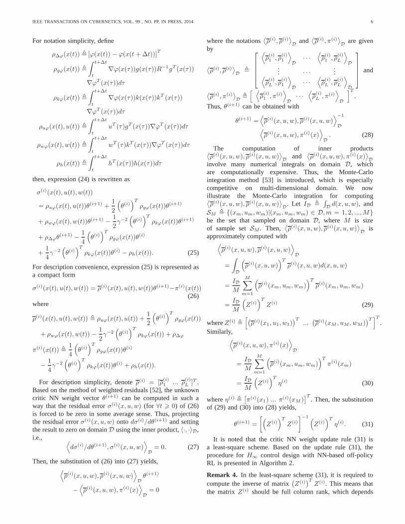
Fig. 1: For the linear F16aircraft plant, the critic NNweights θ(i)1 ∼ θ

(i)3 at each

iteration.

0 1 2 3 4 5−0.5

0

0.5

1

1.5

2

iteration (i)

we

igh

ts (θ

(i) )

θ4(i) θ

5(i) θ

6(i)

Fig. 2: For the linear F16aircraft plant, the critic NNweights θ(i)4 ∼ θ

(i)6 at each

iteration.

function approximation is required for linear systems. Then,by collecting sample setSM for computing ρux, ρwx, ρxxand ρ∆x, a more simpler least-square scheme (31) can bederived to obtain the unknown parameter vectorvec(P (i+1))accordingly.

VI. SIMULATION STUDIES

In this section, the efficiency of the developed NN-basedoff-policy RL method is tested on a F16 aircraft plant. Then,it is applied to the rotational/translational actuator (RTAC)nonlinear benchmark problem.

A. Efficiency test on linear F16 aircraft plant

Consider a F16 aircraft plant that used in [32], [46], [48],[63], where the system dynamics is described by a linearcontinuous-time model:

x =

−1.01887 0.90506 −0.002150.82225 −1.07741 −0.17555

0 0 −1

x

+

001

u+

100

w (49)

z =x. (50)

where the system state vector isx = [α q δe]T , α denotes

the angle of attack,q is the pitch rate andδe is the elevatordeflection angle. The control inputu is the elevator actuatorvoltage and the disturbancew is wind gusts on angle ofattack. SelectR = 1 andγ = 5 for theL2-gain performance(3). Then, solve the associated ARE (41) with the MATLABcommand CARE, we obtain

P =

1.6573 1.3954 −0.16611.3954 1.6573 −0.1804−0.1661 −0.1804 0.4371

.

For linear systems, the solution of the HJI equation isV ∗(x) = xTPx, thus the complete activation function vectorfor critic NN is ϕ(x) =

[x21 x1x2 x1x3 x2

2 x2x3 x23

]Tof

size L = 6. Then, the idea critic NN weight vector isθ∗ = [p11 2p12 2p13 p22 2p23 p33]

T = [1.6573 2.7908−0.3322 1.6573 − 0.3608 0.4371]T . Letting initial critic NNweightθ(0)l = 0(l = 1, ..., 6), iterative stop criterionξ = 10−7

and integral time interval∆t = 0.1s, Algorithm 2 is applied to


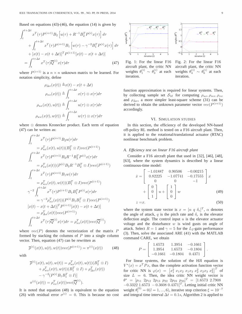
0 1 2 3−1

0

1

2

3

iteration (i)

we

igh

ts (θ

(i) )

θ1(i) θ

2(i) θ

3(i) θ

4(i) θ

5(i)

Fig. 3: For the RTAC sys-tem, the critic NN θ

(i)1 ∼

θ(i)5 weights at each itera-

tion.

0 1 2 3−2

−1.5

−1

−0.5

0

0.5

1

iteration (i)

we

igh

ts (θ

(i) )

θ6(i) θ

7(i) θ

8(i) θ

9(i) θ

10(i)

Fig. 4: For the RTAC sys-tem, the critic NN θ

(i)6 ∼

θ(i)10 weights at each itera-

tion.

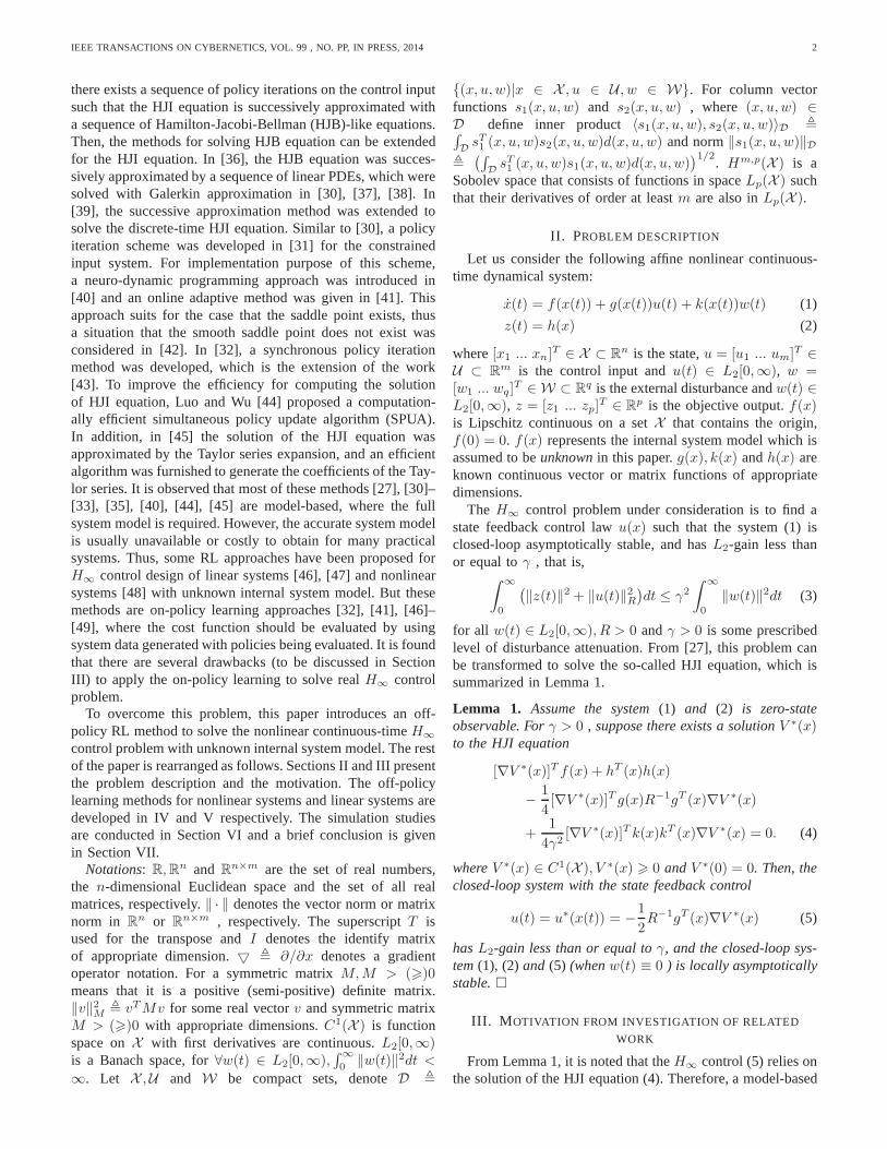
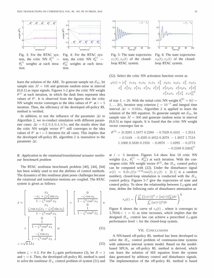
learn the solution of the ARE. To generate sample setSM , letsample sizeM = 100 and generate random noise in interval[0,0.1] as input signals. Figures 1-2 give the critic NN weightθ(i) at each iteration, in which the dash lines represent ideavalues ofθ∗. It is observed from the figures that the criticNN weight vector converges to the idea values ofθ∗ at i = 5iteration. Then, the efficiency of the developed off-policyRLmethod is verified.

In addition, to test the influence of the parameter∆t toAlgorithm 2, we re-conduct simulation with different param-eter cases:∆t = 0.2, 0.3, 0.4, 0.5s, and the results show thatthe critic NN weight vectorθ(i) still converges to the ideavalues ofθ∗ at i = 5 iteration for all cases. This implies thatthe developed off-policy RL algorithm 2 is insensitive to theparameter∆t.

B. Application to the rotational/translational actuator nonlin-ear benchmark problem

The RTAC nonlinear benchmark problem [40], [44], [64]has been widely used to test the abilities of control methods.The dynamics of this nonlinear plant poses challenges becausethe rotational and translation motions are coupled. The RTACsystem is given as follows:

x =

x2

−x1 + ζx24 sinx3

1− ζ2 cos2 x3

x4

ζ cosx3(x1 − ζx24 sinx3)

1− ζ2 cos2 x3

+

0−ζ cosx3

1− ζ2 cos2 x3

01

1− ζ2 cos2 x3

u

+

01

1− ζ2 cos2 x3

0−ζ cosx3

1− ζ2 cos2 x3

w (51)

z =√0.1Ix (52)

whereζ = 0.2. For theL2-gain performance (3), letR = 1andγ = 6. Then, the developed off-policy RL method is usedto solve the nonlinearH∞ control problem of system (51) and

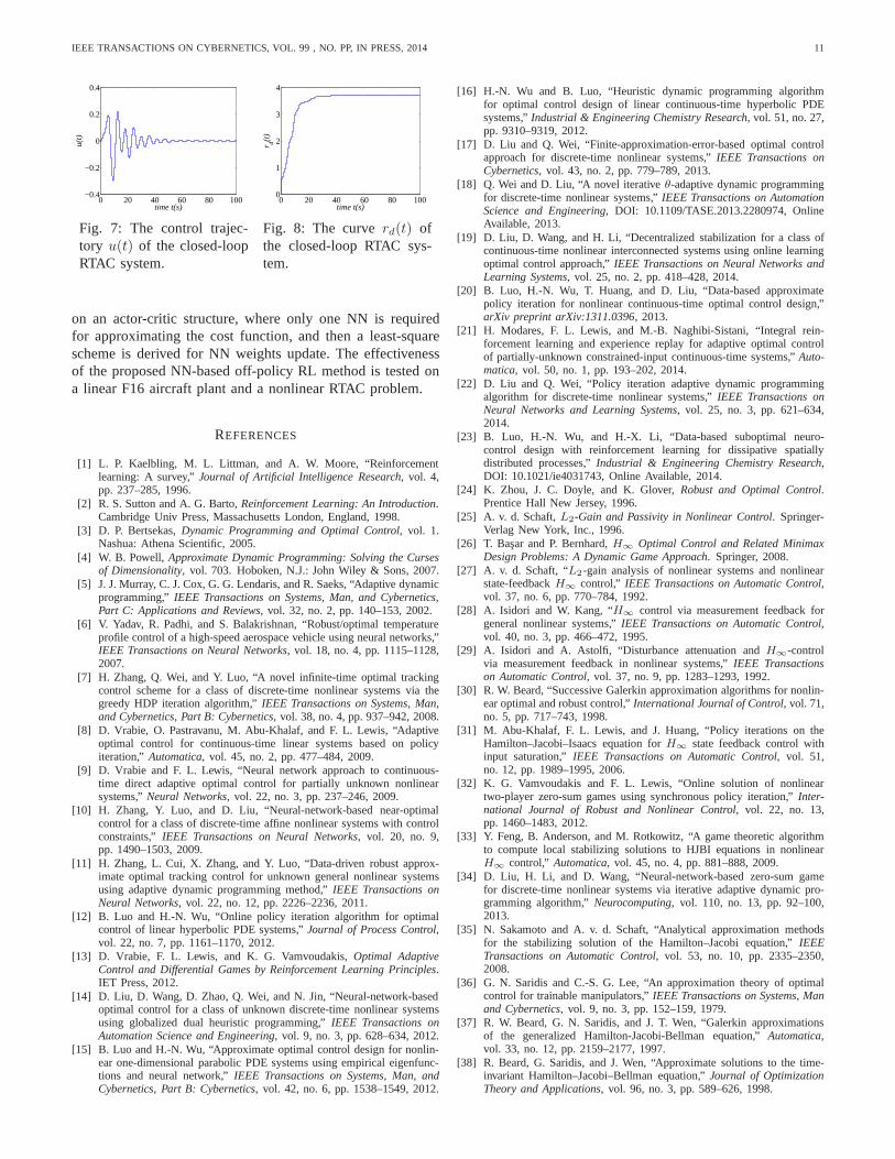
0 20 40 60 80 100−0.4

−0.2

0

0.2

0.4

time t(s)

x1

x2

Fig. 5: The state trajectoriesx1(t), x2(t) of the closed-loop RTAC system.

0 20 40 60 80 100−1

−0.5

0

0.5

1

time t(s)

x3

x4

Fig. 6: The state trajectoriesx3(t), x4(t) of the closed-loop RTAC system.

(52). Select the critic NN activation function vector as

ϕ(x) = [x21 x1x2 x1x3 x1x4 x2

2 x2x3 x2x4 x23 x3x4

x24 x3

1x2 x31x3 x3

1x4 x21x

22 x2

1x2x3 x21x2x4 x2

1x23

x21x3x4 x2

1x24 x1x

32]

T

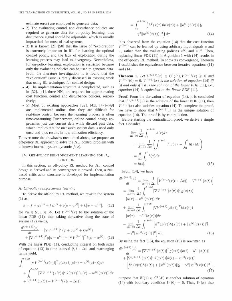
of sizeL = 20. With the initial critic NN weightθ(0)l = 0(l =1, ..., 20), iterative stop criterionξ = 10−7 and integral timeinterval ∆t = 0.033s, Algorithm 2 is applied to learn thesolution of the HJI equation. To generate sample setSM , letsample sizeM = 300 and generate random noise in interval[0,0.5] as input signals. It is found that the critic NN weightvector converges fast to

θ(3) = [0.3285 1.5877 0.2288 − 0.7028 0.4101 − 1.2514

− 0.5448 − 0.4595 0.4852 0.2078 − 1.3857 1.7518

1.1000 0.5820 0.1950 − 0.0978 − 1.0295 − 0.2773

− 0.2169 0.2463]T

at i = 3 iteration. Figures 3-4 show first 10 critic NNweights (i.e.,θ(i)1 ∼ θ

(i)10 ) at each iteration. With the con-

vergent critic NN weight vectorθ(3), theH∞ control policycan be computed with (22). Under the disturbance signalw(t) = 0.2r1(t)e

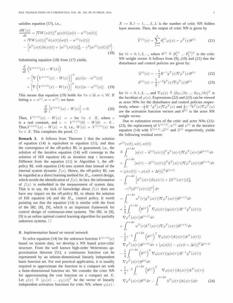
−0.2tcos(t), (r1(t) ∈ [0, 1] is a randomnumber), closed-loop simulation is conducted with theH∞

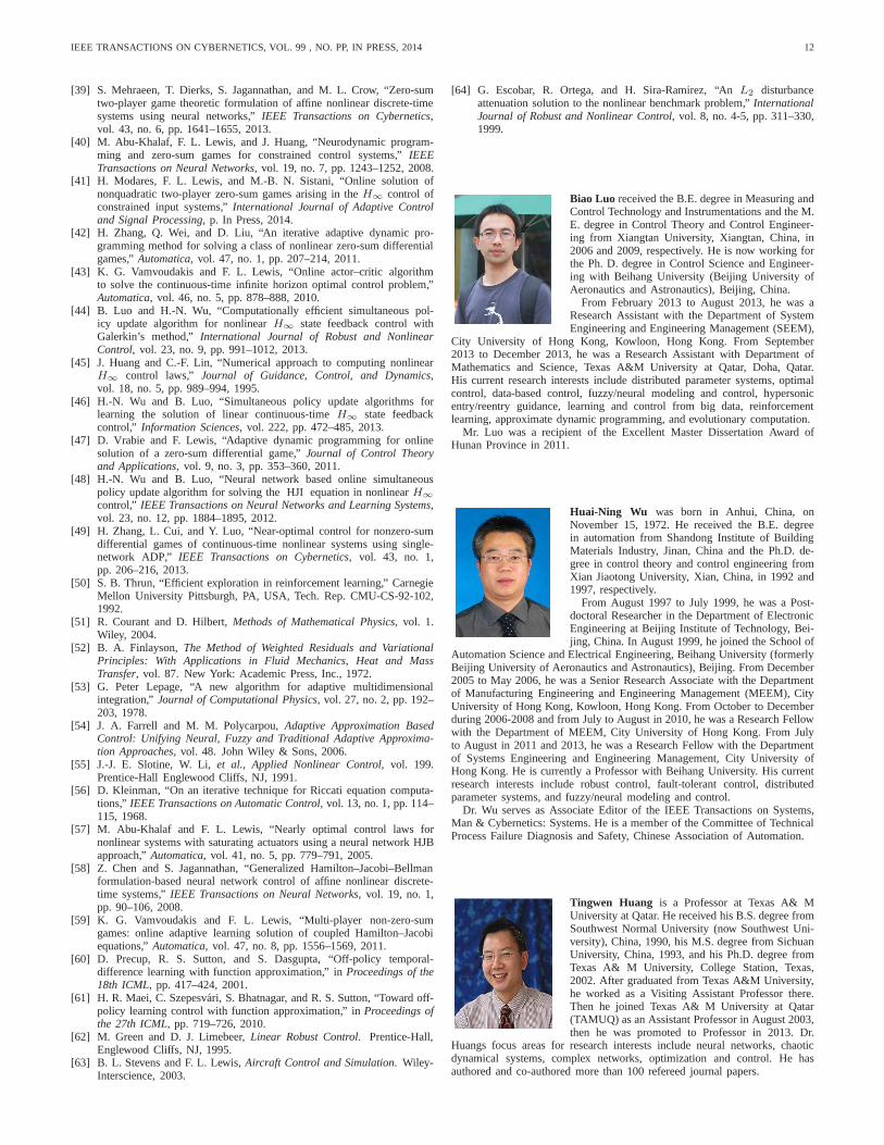
control policy. Figures 5-7 give the trajectories of state andcontrol policy. To show the relationship betweenL2-gain andtime, define the following ratio of disturbance attenuationas

rd(t) =

(∫ t

0

(‖z(τ)‖2 + ‖u(τ)‖2R

)dτ

∫ t

0 ‖w(τ)‖2dτ

) 1

2

.

Figure 8 shows the curve ofrd(t) , where it converges to3.7024(< γ = 6) as time increases, which implies that thedesignedH∞ control law can achieve a prescribedL2-gainperformance levelγ for the closed-loop system.

VII. C ONCLUSIONS

A NN-based off-policy RL method has been developed tosolve theH∞ control problem of continuous-time systemswith unknown internal system model. Based on the model-based SPUA, an off-policy RL method is derived, whichcan learn the solution of HJI equation from the systemdata generated by arbitrary control and disturbance signals.The implementation of the off-policy RL method is based


0 20 40 60 80 100−0.4

−0.2

0

0.2

0.4u

(t)

time t(s)

Fig. 7: The control trajec-tory u(t) of the closed-loopRTAC system.

0 20 40 60 80 1000

1

2

3

4

time t(s)

r d(t)

Fig. 8: The curverd(t) ofthe closed-loop RTAC sys-tem.

on an actor-critic structure, where only one NN is requiredfor approximating the cost function, and then a least-squarescheme is derived for NN weights update. The effectivenessof the proposed NN-based off-policy RL method is tested ona linear F16 aircraft plant and a nonlinear RTAC problem.

REFERENCES

[1] L. P. Kaelbling, M. L. Littman, and A. W. Moore, “Reinforcementlearning: A survey,”Journal of Artificial Intelligence Research, vol. 4,pp. 237–285, 1996.

[2] R. S. Sutton and A. G. Barto,Reinforcement Learning: An Introduction.Cambridge Univ Press, Massachusetts London, England, 1998.

[3] D. P. Bertsekas,Dynamic Programming and Optimal Control, vol. 1.Nashua: Athena Scientific, 2005.

[4] W. B. Powell, Approximate Dynamic Programming: Solving the Cursesof Dimensionality, vol. 703. Hoboken, N.J.: John Wiley & Sons, 2007.

[5] J. J. Murray, C. J. Cox, G. G. Lendaris, and R. Saeks, “Adaptive dynamicprogramming,”IEEE Transactions on Systems, Man, and Cybernetics,Part C: Applications and Reviews, vol. 32, no. 2, pp. 140–153, 2002.

[6] V. Yadav, R. Padhi, and S. Balakrishnan, “Robust/optimal temperatureprofile control of a high-speed aerospace vehicle using neural networks,”IEEE Transactions on Neural Networks, vol. 18, no. 4, pp. 1115–1128,2007.

[7] H. Zhang, Q. Wei, and Y. Luo, “A novel infinite-time optimal trackingcontrol scheme for a class of discrete-time nonlinear systems via thegreedy HDP iteration algorithm,”IEEE Transactions on Systems, Man,and Cybernetics, Part B: Cybernetics, vol. 38, no. 4, pp. 937–942, 2008.

[8] D. Vrabie, O. Pastravanu, M. Abu-Khalaf, and F. L. Lewis,“Adaptiveoptimal control for continuous-time linear systems based on policyiteration,” Automatica, vol. 45, no. 2, pp. 477–484, 2009.

[9] D. Vrabie and F. L. Lewis, “Neural network approach to continuous-time direct adaptive optimal control for partially unknownnonlinearsystems,”Neural Networks, vol. 22, no. 3, pp. 237–246, 2009.

[10] H. Zhang, Y. Luo, and D. Liu, “Neural-network-based near-optimalcontrol for a class of discrete-time affine nonlinear systems with controlconstraints,” IEEE Transactions on Neural Networks, vol. 20, no. 9,pp. 1490–1503, 2009.

[11] H. Zhang, L. Cui, X. Zhang, and Y. Luo, “Data-driven robust approx-imate optimal tracking control for unknown general nonlinear systemsusing adaptive dynamic programming method,”IEEE Transactions onNeural Networks, vol. 22, no. 12, pp. 2226–2236, 2011.

[12] B. Luo and H.-N. Wu, “Online policy iteration algorithmfor optimalcontrol of linear hyperbolic PDE systems,”Journal of Process Control,vol. 22, no. 7, pp. 1161–1170, 2012.

[13] D. Vrabie, F. L. Lewis, and K. G. Vamvoudakis,Optimal AdaptiveControl and Differential Games by Reinforcement Learning Principles.IET Press, 2012.

[14] D. Liu, D. Wang, D. Zhao, Q. Wei, and N. Jin, “Neural-network-basedoptimal control for a class of unknown discrete-time nonlinear systemsusing globalized dual heuristic programming,”IEEE Transactions onAutomation Science and Engineering, vol. 9, no. 3, pp. 628–634, 2012.

[15] B. Luo and H.-N. Wu, “Approximate optimal control design for nonlin-ear one-dimensional parabolic PDE systems using empiricaleigenfunc-tions and neural network,”IEEE Transactions on Systems, Man, andCybernetics, Part B: Cybernetics, vol. 42, no. 6, pp. 1538–1549, 2012.

[16] H.-N. Wu and B. Luo, “Heuristic dynamic programming algorithmfor optimal control design of linear continuous-time hyperbolic PDEsystems,”Industrial & Engineering Chemistry Research, vol. 51, no. 27,pp. 9310–9319, 2012.

[17] D. Liu and Q. Wei, “Finite-approximation-error-basedoptimal controlapproach for discrete-time nonlinear systems,”IEEE Transactions onCybernetics, vol. 43, no. 2, pp. 779–789, 2013.

[18] Q. Wei and D. Liu, “A novel iterativeθ-adaptive dynamic programmingfor discrete-time nonlinear systems,”IEEE Transactions on AutomationScience and Engineering, DOI: 10.1109/TASE.2013.2280974, OnlineAvailable, 2013.

[19] D. Liu, D. Wang, and H. Li, “Decentralized stabilization for a class ofcontinuous-time nonlinear interconnected systems using online learningoptimal control approach,”IEEE Transactions on Neural Networks andLearning Systems, vol. 25, no. 2, pp. 418–428, 2014.

[20] B. Luo, H.-N. Wu, T. Huang, and D. Liu, “Data-based approximatepolicy iteration for nonlinear continuous-time optimal control design,”arXiv preprint arXiv:1311.0396, 2013.

[21] H. Modares, F. L. Lewis, and M.-B. Naghibi-Sistani, “Integral rein-forcement learning and experience replay for adaptive optimal controlof partially-unknown constrained-input continuous-timesystems,”Auto-matica, vol. 50, no. 1, pp. 193–202, 2014.

[22] D. Liu and Q. Wei, “Policy iteration adaptive dynamic programmingalgorithm for discrete-time nonlinear systems,”IEEE Transactions onNeural Networks and Learning Systems, vol. 25, no. 3, pp. 621–634,2014.

[23] B. Luo, H.-N. Wu, and H.-X. Li, “Data-based suboptimal neuro-control design with reinforcement learning for dissipative spatiallydistributed processes,”Industrial & Engineering Chemistry Research,DOI: 10.1021/ie4031743, Online Available, 2014.

[24] K. Zhou, J. C. Doyle, and K. Glover,Robust and Optimal Control.Prentice Hall New Jersey, 1996.

[25] A. v. d. Schaft,L2-Gain and Passivity in Nonlinear Control. Springer-Verlag New York, Inc., 1996.

[26] T. Basar and P. Bernhard,H∞ Optimal Control and Related MinimaxDesign Problems: A Dynamic Game Approach. Springer, 2008.

[27] A. v. d. Schaft, “L2-gain analysis of nonlinear systems and nonlinearstate-feedbackH∞ control,” IEEE Transactions on Automatic Control,vol. 37, no. 6, pp. 770–784, 1992.

[28] A. Isidori and W. Kang, “H∞ control via measurement feedback forgeneral nonlinear systems,”IEEE Transactions on Automatic Control,vol. 40, no. 3, pp. 466–472, 1995.

[29] A. Isidori and A. Astolfi, “Disturbance attenuation andH∞-controlvia measurement feedback in nonlinear systems,”IEEE Transactionson Automatic Control, vol. 37, no. 9, pp. 1283–1293, 1992.

[30] R. W. Beard, “Successive Galerkin approximation algorithms for nonlin-ear optimal and robust control,”International Journal of Control, vol. 71,no. 5, pp. 717–743, 1998.

[31] M. Abu-Khalaf, F. L. Lewis, and J. Huang, “Policy iterations on theHamilton–Jacobi–Isaacs equation forH∞ state feedback control withinput saturation,”IEEE Transactions on Automatic Control, vol. 51,no. 12, pp. 1989–1995, 2006.

[32] K. G. Vamvoudakis and F. L. Lewis, “Online solution of nonlineartwo-player zero-sum games using synchronous policy iteration,” Inter-national Journal of Robust and Nonlinear Control, vol. 22, no. 13,pp. 1460–1483, 2012.

[33] Y. Feng, B. Anderson, and M. Rotkowitz, “A game theoretic algorithmto compute local stabilizing solutions to HJBI equations innonlinearH∞ control,” Automatica, vol. 45, no. 4, pp. 881–888, 2009.

[34] D. Liu, H. Li, and D. Wang, “Neural-network-based zero-sum gamefor discrete-time nonlinear systems via iterative adaptive dynamic pro-gramming algorithm,”Neurocomputing, vol. 110, no. 13, pp. 92–100,2013.

[35] N. Sakamoto and A. v. d. Schaft, “Analytical approximation methodsfor the stabilizing solution of the Hamilton–Jacobi equation,” IEEETransactions on Automatic Control, vol. 53, no. 10, pp. 2335–2350,2008.

[36] G. N. Saridis and C.-S. G. Lee, “An approximation theoryof optimalcontrol for trainable manipulators,”IEEE Transactions on Systems, Manand Cybernetics, vol. 9, no. 3, pp. 152–159, 1979.

[37] R. W. Beard, G. N. Saridis, and J. T. Wen, “Galerkin approximationsof the generalized Hamilton-Jacobi-Bellman equation,”Automatica,vol. 33, no. 12, pp. 2159–2177, 1997.

[38] R. Beard, G. Saridis, and J. Wen, “Approximate solutions to the time-invariant Hamilton–Jacobi–Bellman equation,”Journal of OptimizationTheory and Applications, vol. 96, no. 3, pp. 589–626, 1998.

http://arxiv.org/abs/1311.0396


[39] S. Mehraeen, T. Dierks, S. Jagannathan, and M. L. Crow, “Zero-sumtwo-player game theoretic formulation of affine nonlinear discrete-timesystems using neural networks,”IEEE Transactions on Cybernetics,vol. 43, no. 6, pp. 1641–1655, 2013.

[40] M. Abu-Khalaf, F. L. Lewis, and J. Huang, “Neurodynamicprogram-ming and zero-sum games for constrained control systems,”IEEETransactions on Neural Networks, vol. 19, no. 7, pp. 1243–1252, 2008.

[41] H. Modares, F. L. Lewis, and M.-B. N. Sistani, “Online solution ofnonquadratic two-player zero-sum games arising in theH∞ control ofconstrained input systems,”International Journal of Adaptive Controland Signal Processing, p. In Press, 2014.

[42] H. Zhang, Q. Wei, and D. Liu, “An iterative adaptive dynamic pro-gramming method for solving a class of nonlinear zero-sum differentialgames,”Automatica, vol. 47, no. 1, pp. 207–214, 2011.

[43] K. G. Vamvoudakis and F. L. Lewis, “Online actor–criticalgorithmto solve the continuous-time infinite horizon optimal control problem,”Automatica, vol. 46, no. 5, pp. 878–888, 2010.

[44] B. Luo and H.-N. Wu, “Computationally efficient simultaneous pol-icy update algorithm for nonlinearH∞ state feedback control withGalerkin’s method,” International Journal of Robust and NonlinearControl, vol. 23, no. 9, pp. 991–1012, 2013.

[45] J. Huang and C.-F. Lin, “Numerical approach to computing nonlinearH∞ control laws,” Journal of Guidance, Control, and Dynamics,vol. 18, no. 5, pp. 989–994, 1995.

[46] H.-N. Wu and B. Luo, “Simultaneous policy update algorithms forlearning the solution of linear continuous-timeH∞ state feedbackcontrol,” Information Sciences, vol. 222, pp. 472–485, 2013.

[47] D. Vrabie and F. Lewis, “Adaptive dynamic programming for onlinesolution of a zero-sum differential game,”Journal of Control Theoryand Applications, vol. 9, no. 3, pp. 353–360, 2011.

[48] H.-N. Wu and B. Luo, “Neural network based online simultaneouspolicy update algorithm for solving the HJI equation in nonlinearH∞

control,” IEEE Transactions on Neural Networks and Learning Systems,vol. 23, no. 12, pp. 1884–1895, 2012.

[49] H. Zhang, L. Cui, and Y. Luo, “Near-optimal control for nonzero-sumdifferential games of continuous-time nonlinear systems using single-network ADP,” IEEE Transactions on Cybernetics, vol. 43, no. 1,pp. 206–216, 2013.

[50] S. B. Thrun, “Efficient exploration in reinforcement learning,” CarnegieMellon University Pittsburgh, PA, USA, Tech. Rep. CMU-CS-92-102,1992.

[51] R. Courant and D. Hilbert,Methods of Mathematical Physics, vol. 1.Wiley, 2004.

[52] B. A. Finlayson,The Method of Weighted Residuals and VariationalPrinciples: With Applications in Fluid Mechanics, Heat andMassTransfer, vol. 87. New York: Academic Press, Inc., 1972.

[53] G. Peter Lepage, “A new algorithm for adaptive multidimensionalintegration,”Journal of Computational Physics, vol. 27, no. 2, pp. 192–203, 1978.

[54] J. A. Farrell and M. M. Polycarpou,Adaptive Approximation BasedControl: Unifying Neural, Fuzzy and Traditional Adaptive Approxima-tion Approaches, vol. 48. John Wiley & Sons, 2006.

[55] J.-J. E. Slotine, W. Li,et al., Applied Nonlinear Control, vol. 199.Prentice-Hall Englewood Cliffs, NJ, 1991.

[56] D. Kleinman, “On an iterative technique for Riccati equation computa-tions,” IEEE Transactions on Automatic Control, vol. 13, no. 1, pp. 114–115, 1968.

[57] M. Abu-Khalaf and F. L. Lewis, “Nearly optimal control laws fornonlinear systems with saturating actuators using a neuralnetwork HJBapproach,”Automatica, vol. 41, no. 5, pp. 779–791, 2005.

[58] Z. Chen and S. Jagannathan, “Generalized Hamilton–Jacobi–Bellmanformulation-based neural network control of affine nonlinear discrete-time systems,”IEEE Transactions on Neural Networks, vol. 19, no. 1,pp. 90–106, 2008.

[59] K. G. Vamvoudakis and F. L. Lewis, “Multi-player non-zero-sumgames: online adaptive learning solution of coupled Hamilton–Jacobiequations,”Automatica, vol. 47, no. 8, pp. 1556–1569, 2011.

[60] D. Precup, R. S. Sutton, and S. Dasgupta, “Off-policy temporal-difference learning with function approximation,” inProceedings of the18th ICML, pp. 417–424, 2001.

[61] H. R. Maei, C. Szepesvari, S. Bhatnagar, and R. S. Sutton, “Toward off-policy learning control with function approximation,” inProceedings ofthe 27th ICML, pp. 719–726, 2010.

[62] M. Green and D. J. Limebeer,Linear Robust Control. Prentice-Hall,Englewood Cliffs, NJ, 1995.

[63] B. L. Stevens and F. L. Lewis,Aircraft Control and Simulation. Wiley-Interscience, 2003.

[64] G. Escobar, R. Ortega, and H. Sira-Ramirez, “AnL2 disturbanceattenuation solution to the nonlinear benchmark problem,”InternationalJournal of Robust and Nonlinear Control, vol. 8, no. 4-5, pp. 311–330,1999.

Biao Luo received the B.E. degree in Measuring andControl Technology and Instrumentations and the M.E. degree in Control Theory and Control Engineer-ing from Xiangtan University, Xiangtan, China, in2006 and 2009, respectively. He is now working forthe Ph. D. degree in Control Science and Engineer-ing with Beihang University (Beijing University ofAeronautics and Astronautics), Beijing, China.

From February 2013 to August 2013, he was aResearch Assistant with the Department of SystemEngineering and Engineering Management (SEEM),

City University of Hong Kong, Kowloon, Hong Kong. From September2013 to December 2013, he was a Research Assistant with Department ofMathematics and Science, Texas A&M University at Qatar, Doha, Qatar.His current research interests include distributed parameter systems, optimalcontrol, data-based control, fuzzy/neural modeling and control, hypersonicentry/reentry guidance, learning and control from big data, reinforcementlearning, approximate dynamic programming, and evolutionary computation.

Mr. Luo was a recipient of the Excellent Master DissertationAward ofHunan Province in 2011.

Huai-Ning Wu was born in Anhui, China, onNovember 15, 1972. He received the B.E. degreein automation from Shandong Institute of BuildingMaterials Industry, Jinan, China and the Ph.D. de-gree in control theory and control engineering fromXian Jiaotong University, Xian, China, in 1992 and1997, respectively.

From August 1997 to July 1999, he was a Post-doctoral Researcher in the Department of ElectronicEngineering at Beijing Institute of Technology, Bei-jing, China. In August 1999, he joined the School of

Automation Science and Electrical Engineering, Beihang University (formerlyBeijing University of Aeronautics and Astronautics), Beijing. From December2005 to May 2006, he was a Senior Research Associate with the Departmentof Manufacturing Engineering and Engineering Management (MEEM), CityUniversity of Hong Kong, Kowloon, Hong Kong. From October toDecemberduring 2006-2008 and from July to August in 2010, he was a Research Fellowwith the Department of MEEM, City University of Hong Kong. From Julyto August in 2011 and 2013, he was a Research Fellow with the Departmentof Systems Engineering and Engineering Management, City University ofHong Kong. He is currently a Professor with Beihang University. His currentresearch interests include robust control, fault-tolerant control, distributedparameter systems, and fuzzy/neural modeling and control.

Dr. Wu serves as Associate Editor of the IEEE Transactions onSystems,Man & Cybernetics: Systems. He is a member of the Committee ofTechnicalProcess Failure Diagnosis and Safety, Chinese Associationof Automation.

Tingwen Huang is a Professor at Texas A& MUniversity at Qatar. He received his B.S. degree fromSouthwest Normal University (now Southwest Uni-versity), China, 1990, his M.S. degree from SichuanUniversity, China, 1993, and his Ph.D. degree fromTexas A& M University, College Station, Texas,2002. After graduated from Texas A&M University,he worked as a Visiting Assistant Professor there.Then he joined Texas A& M University at Qatar(TAMUQ) as an Assistant Professor in August 2003,then he was promoted to Professor in 2013. Dr.

Huangs focus areas for research interests include neural networks, chaoticdynamical systems, complex networks, optimization and control. He hasauthored and co-authored more than 100 refereed journal papers.

Documents

IEEE TRANSACTIONS ON CYBERNETICS, VOL. 99 , NO. PP, IN