IEEE TRANSACTIONS ON SYSTEMS, MAN, AND CYBERNETICS… Saliency... · IEEE TRANSACTIONS ON SYSTEMS, MAN, AND CYBERNETICS—PART B: CYBERNETICS 1 Saliency Detection by Multiple Instance

IEEE TRANSACTIONS ON SYSTEMS, MAN, AND CYBERNETICS—PART B: CYBERNETICS 1

Saliency Detection by Multiple Instance LearningQi Wang, Yuan Yuan, Senior Member, IEEE, Pingkun Yan, Senior Member, IEEE, and Xuelong Li, Fellow, IEEE

Abstract

Saliency detection has been a hot topic in recent years. Its popularity is mainly because of its theoretical meaning for explaining

human attention and applicable aims in segmentation, recognition, etc. Nevertheless, traditional algorithms are mostly based on

unsupervised techniques, which have limited learning ability. The obtained saliency map is also inconsistent with many properties

of human behavior. In order to overcome the challenges of inability and inconsistency, this paper presents a framework based

on multiple instance learning. Low-, mid-, and high-level features are incorporated in the detection procedure and the learning

ability enables it robust to noise. Experiments on a dataset containing 1,000 images demonstrate the effectiveness of the proposed

framework. Its applicability is shown in the context of a seam carving application.

Index Terms

Computer vision, machine learning, saliency, attention, saliency map, multiple instance learning.

I. INTRODUCTION

THE human visual system pays inequal attention to what is seen in the world. For instance, when looking at images in

Fig. 1, people are usually attracted by some particular objects within them (i.e., flower, boat, and dog, respectively).

Other subjects appear to be uninteresting for observers. This ability of “withdraw from some things in order to deal effectively

with others” is called attention [1][2].

Research on visual attention has found use in many applications, e.g., object recognition [3][4][5][6], image segmentation

[7][8], content-based retargeting [9], image retrieval [10], adaptive image display [11], and advertising design [12]. Because

of these applications, extensive efforts from different disciplines have been spent towards visual attention, including computer

vision [13][14][15][16][17], cognitive psychology [18], psychophysics [19], and neurobiology [20]. However, though the ability

of selective attention seems to be natural to humans, the mechanisms behind this phenomenon are unclear. In this paper, one

particular aspect of visual attention is explored from a computer vision viewpoint–saliency detection.

The task of saliency detection is to extract the salient objects in an image, assuming that there is one or several salient

ones within it. It is mainly approached by three steps, feature selection, saliency calculation and map normalization. First, low

level features, such as color, intensity, orientation, and motion, are selected as the basic elements for supporting the saliency

detection. Second, the saliency value for each pixel in an input image is calculated according to a predefined model. In the

end, saliency maps from different sources are integrated and normalized to get a final result. The saliency value is generally

The authors are with the Center for OPTical IMagery Analysis and Learning (OPTIMAL), State Key Laboratory of Transient Optics and Photonics, XianInstitute of Optics and Precision Mechanics, Chinese Academy of Sciences, Xian 710119, Shaanxi, P. R. China (e-mail: [email protected]; [email protected];[email protected]; xuelong [email protected]).


Fig. 1. Saliency detection. From top to bottom, each row respectively represents the original images, the saliency maps calculated by CA [15], and thesaliency maps calculated by the proposed framework.

denoted by a number scaled to [0, 1] and shown in a gray image. The greater value the pixel has, the higher possibility it is

of being salient. A typical example of saliency detection results is illustrated in the middle row of Fig. 1.

Similar to existing algorithms, the general procedure for saliency detection is also followed in this paper; Unlike to existing

algorithms, it is conducted in a different framework, multiple instance learning (MIL) [21].

A. Related Work

Algorithms for saliency detection can be generally categorized as model based and computation based.

• Model based algorithms adopt a top-down route. In these algorithms, a high level model is first established empirically.

Then the subsequent calculation is conducted with respect to the defined model. The work by Koch and Ullman [22]

is among the earliest attempts of this kind. They proposed a bionics model to intimate an attention shift of human and

primate. In their implementation, a neuron-like network is employed to combine several topographical parallel saliency

maps from different image clues. Then a Winner-Take-All mechanism keeps the selective attention point drifting from

one conspicuous location to another. Another architecture, probably the most influential one, is the work by Itti et al.

[23]. Inspired by the early vision of primates, they extract multi-scale features through a set of linear “center surround”

operations. Then the “focus of attention” is determined by combining and normalizing the across-scale maps. Based on

this, Walther et al. [6] presented a combined model for spatial attention and object recognition, in which the entire visual


field is considered but only part of it is sufficient for recognition. They report that the approach yields encouraging results

and is biologically and applicably plausible.

Different from the above three biologically inspired models, Hou and Zhang [24] tackled the saliency problem from the

spectral residual domain. Through a statistical and experimental analysis, they find that the log-spectrum of natural images

share a similar trend whereby the regions corresponding to singular points in the statistical curves are responsible for the

anomalous ones that count for saliency. Besides that, there are still other algorithms treating this problem with machine

learning approaches. Liu et al. [25] formulated saliency detection in a Markov Random Field (MRF) framework. Model

parameters are learned on a labeled dataset and the static and sequential images are tested afterwards to demonstrate its

effectiveness. Judd et al. [26] dealt with saliency by a Support Vector Machine (SVM), assuming that the saliency level

can be determined by the distance to the decision boundary. Linear kernels are selected to train the involved parameters

and the results are evaluated on a dataset containing 1,003 eye tracking images.

• Computation based algorithms, on the contrary, follow a bottom-up route. Saliency of this type is typically calculated by

contrast from low level features. For example, Wang and Li [27] proposed a two-stage approach for saliency detection.

In the first stage, the spectrum residual model [24] is extended by introducing two modules–automatic channel selection

and decision reversal. In the second stage, incomplete salient regions are propagated based on the basic Gestalt grouping

principles. Achanta et al. [16] presented an algorithm that outputs saliency maps with well-defined boundaries of salient

objects, which are obtained by retaining more frequency content from the input image than previous techniques. They

also constructed a dataset containing labeled segmentation of 1,000 images to be used as ground truth. Later, Achanta and

Susstrucnk [28] detected saliency with respect to the hypothesis that the scale of an object relates to the image borders.

They thus varied the bandwidth of the center surround-filtering near image borders using symmetric surrounds to detect

saliency. Zhang et al. [29] provided a Bayesian expression of the saliency task. Self-information and pointwise mutual

information are fused to generate a final result. Harel et al. [30] designed a graph based algorithm consisting of two

steps: first forming activation maps on certain feature channels, and then combining them in a manner that highlights

conspicuity. It is claimed that the model is mathematically simple and practically plausible. Cheng et al. [31] brought in

a region based concept that simultaneously evaluates global contrast difference and spatial coherence.

Besides various techniques involved in the detection procedure, there are other algorithms trying to get a novel definition

for saliency. Goferman et al. [15] proposed a new type of saliency called context-aware saliency which aims at extracting

the image regions representing the scene, while previous definitions sought to identify fixation points or the dominant

objects. Chang et al. [17] defined the salient region not only from the distinctiveness of a single image, but also considering

the repeatedness among images. Wang et al. [32] considered saliency as an anomaly with respect to a given context, which

can be global or local. The global context is estimated in the whole image relative to a bunch of images. In the local

context, the input image is partitioned into patches and saliency in each patch is computed by contrast to other patches.


B. Limitations of Existing Algorithms

Though various algorithms for saliency detection have been presented in the past few years, and good performance for

predicting human fixations in viewing images has been achieved in some circumstances, there are still limitations.

Lack of full resolution. The saliency maps of several algorithms suffer from low resolution. For example, the map by Itti et

al. [23] is 256 times smaller than the original image, and the one by Hou and Zhang [24] is fixed by 64 pixels in width (or

height). This will lead to a limited applicability in some situations such as segmentation and recognition.

Inconsistency. Most existing algorithms generate inconsistent saliency maps, which is undesirable. Some of these have fuzzy

maps with ill-defined boundaries. Some others highlight object boundaries but fail to detect the whole target region. There are

still others emphasizing smaller salient regions other than the whole desired one. This inconsistency makes the detection task

less fulfilled and limits the usefulness in certain applications.

The above two limitations are mainly derived from the following reasons.

First, not all image clues are utilized for supporting saliency calculation. Humans perceive the world not only by color,

but also by other types of clues such as texture, shape, depth, shadow, and motion. This rule of perceiving is true for visual

attention processing [22]. Nevertheless, to the best of the authors’ knowledge, color is probably the most frequently employed

feature in existing work of saliency detection. Besides that, motion and spectrum has been less explored in [16][33]. Other

clues such as texture, boundary, shape, etc. are rarely considered.

Second, existing models have not well considered the learning ability of humans. Previous works are in general based on

single image contrast. The consequently derived model is mostly heuristic. This makes the machine independent of learning

ability, to which the human attention is closely related. Recently, learning based algorithms seem to be generating encouraging

results. But there are still problems to be solved. For example, saliency maps of Judd et al. [26] were learned from a SVM

classifier. The dataset employed in training is composed of images with ground truth fixation points instead of regions.

Sometimes, a few fixation points may be adequate to use. But most of the time, the desired results are salient regions. Liu

et al. [34] proposed to detect saliency by MRF. Though the involved parameters are learned from labeled images, no higher

level features are incorporated. Besides, the training images are labeled with rectangles larger than the actual salient objects.

This makes the model less accurate.

C. The Proposed Framework

In this paper, a saliency detection framework based on multiple instance learning is presented. It is aimed to overcome the

challenge that we do not know but have to detect the salient object in an input image.

First, different from existing techniques, the detection procedure is modeled as a MIL problem, where segmented regions are

taken as bags and the sampled points within them as instances. Second, more features, including low-, mid-, and high-level,

are incorporated into the learning and testing process. They are position, color, texture, scale, center prior, and boundary.

Since humans recognize the world by integrated sources of data, the addition of other types of information, not only color and

brightness, might be helpful. In the end, performance is evaluated on a dataset of 1,000 images with four MIL implementations.


The remainder of this paper is organized as follows. Section II formulates the saliency detection task as a MIL problem.

Section III gives a detailed description of the distinctive features employed in the framework. Experimental results are shown

in Section IV and an image retargeting application is demonstrated in Section V. Section VI discusses several issues related

to the proposed algorithm. Section VII concludes the paper.

II. FORMULATION

Multiple instance learning (MIL) is a kind of learning technique with incomplete knowledge about the labels of training

examples. Unlike standard supervised learning, in which each training instance has a known label, the examples here are bags

of instances. Each bag receives a single label and the label of each instance is not necessarily known. A positive bag means at

least one instance in the bag is positive, while a negative bag indicates that all instances in the bag are negative. The objective

of MIL is to classify unseen bags or instances based on the labeled bags in the training data.

Since the seminal work of Dietterich et al. [21], MIL has been researched a lot [35][36]. Early work of this subject is mainly

for the boolean labeled problem. That means the learning result is either 0 or 1. After the introduction of real-valued labels

[37], i.e., the label is in the range of [0, 1], MIL has achieved greater popularity in many applications. This is chiefly due to

its tolerance to the ambiguity of the training data. For example, Viola et al. [38] claimed that object detection had inherent

ambiguities for traditional supervised learning algorithms. For this reason, they adopt the use of MIL in their face detection

algorithm. Babenko et al. [39] made an analogous argument and thus proposed to use a MIL based model for object tracking.

In this paper, the question to be addressed is that we know there must be at least one salient object in the image, but we

don’t know exactly where it is. Therefore, saliency detection is explicitly acknowledged as an innate MIL problem. Existing

learning based algorithms [26][34] tackle this problem pixel by pixel. In order to maintain the consistency of the resulting

saliency maps, it is processed region by region instead. Each image is composed of tens of regions (bags) and each region

consists of numerous pixels (instances). The bag’s degree of being salient is determined according to its belonged instances.

This is typical MIL problem.

A. Definition

Traditional learning algorithms for estimating p(y|x) require a training dataset of the form {⟨x1, y1⟩, . . . , ⟨xn, yn⟩}, where

xi is an instance and yi ∈ {0, 1} is its binary label. In MIL, the training data can be denoted as T = {⟨B1, ℓ1⟩, . . . , ⟨Bb, ℓb⟩},

where Bi is a bag and ℓi is its corresponding binary label. Let Bij be the jth instance of bag i and Bijk the value of instance

Bij on feature k. By learning the correlation between bags and instances, a model can be obtained, according to which each

instance in the testing data receives a real-valued label. The predicted label is defined as

ℓi = maxj

(ℓij), (1)

where ℓij is the instance label, which is not known during training. In summary, the saliency detection problem is formulated

as:


Given an image I, its corresponding bags and instances are first extracted. Then the classification model is learned by MIL.

For a future testing image, its bag label is decided according to the obtained model.

B. Learning Saliency Detection Model

Different techniques can be employed for MIL. In this paper, four widely spread algorithms are selected as an example for

the proposed framework. They are respectively APR [21], EMDD [40], Bag-SVM, and Inst-SVM [35].

APR. APR [21] is the first class of algorithms that were proposed to approach the MIL problem. It aims to find an axis-

parallel hyper-rectangle (APR) that contains at least one instance from every positive bag and no instances from any negative

bag. This is achieved by starting with a point in the feature space and growing it to a minimum rectangle.

EMDD. The basic idea of EMDD [40] is to model the label of each bag with a hidden variable, which is estimated by the

Expectation Maximization (EM) algorithm. It combines the EM algorithm with the Diverse Density (DD) algorithm [41][42]

to search for the maximum likelihood hypothesis. It is defined as

h∗ = argmaxh

P (h|T )

= argminh

b∑i=1

(− logP (ℓi|h,Bi)), (2)

where h is the concept space and h∗ is the concept point to be learned.

Bag-SVM & Inst-SVM. The SVM based algorithm [35] is trying to maximize the soft margin between two types of bags

or instances, which leads to Bag-SVM and Inst-SVM. It looks for an linear discriminant such that there is at least one instance

from every positive bag in the positive halfspace, while all instances belonging to negative bags are in the negative halfspace.

It follows the general prototype of SVM and is defined a

minw,b,ξ

1

2∥ w ∥2 +C

∑i

ξi

s.t. ∀i : ℓi maxj

(⟨w, Bij⟩+ b) ≥ 1− ξi. (3)

C. Algorithm Overview

To learn the models by the above four algorithms, training data is constructed from 200 images with ground truth delineation

of salient objects (The dataset will be explained in detail in Section IV). The training procedure is as follows. For each image,

it is first segmented into distinct regions by a mean-shift algorithm [43], which are then treated as bags. Then instances are

randomly sampled from the bag. To keep the efficiency and feasibility, only one percent of the pixels within the bag are

sparsely chosen as its instances. The bag will be labeled positive if there is at least one positive instance; and negative if all

instances are negative. After that, the parameters of the above four algorithms are trained on these labeled bags. For the testing

stage, bags and instances are similarly obtained first. Then the previous trained models are utilized to determine the saliency

for each bag. To have a clear overview of the proposed algorithm, pseudo code is listed as follows:


Algorithm 1 Saliency Detection by MILInput:Training images Ii(i ∈ [1, 200]).Ground truth saliency for each image.Training Stage:

1: for each image Ii(i ∈ [1, 200]) in the training set do2: Segment Ii by mean-shift algorithm to get bags.3: Sample instances within each bag.4: Extract feature vector for each instance.5: end for6: Train the classifier with the feature vectors by APR, EMDD, Bag-SVM, and Inst-SVM.

Testing Stage:1: for each image Ij(j ∈ [1, 800]) in the testing set do2: Segment Ij by mean-shift algorithm to get bags.3: Sample instances within each bag.4: Extract feature vector for each instance.5: Calculate saliency of each bag according to the learned model.6: end for

Output: detected saliency maps.

III. IMAGE FEATURES FOR SALIENCY DEFINITION

The proposed framework for saliency detection have utilized low-, mid-, and high-level features. They are position, color,

texture, scale, center prior, and boundary. Parameters with respect to these features are calibrated according to the training

data. After obtaining all these features, a vector concatenating each feature output is formed to train and test the classifier by

MIL.

A. Low-level Feature

Position. The spatially connected pixels are prone to share similar saliency, while pixels far away tend to be differently

salient. Therefore, the position of each instance is an essential factor for keeping the saliency consistent. Since the sizes of

images differ, the absolute horizontal and vertical position is not suitable for an optimal feature. To avoid this problem, the

normalized position within the range of [0,1]is adopted to ensure that the measurement with respect to different images are

comparable.

Color. This is the most frequently employed feature. Almost every algorithm for saliency detection will refer to it as the

major supporting information for saliency calculation. However, for the choice of color spaces, there is not a noncontroversial

agreement. Some algorithms propose to use L∗a∗b∗ space because it is perceptually meaningful. Others claim the RGB space

is more suitable for this task, because it is computationally efficient. There is still no experimental justification for different

choices. In this paper, three typical color spaces are taken respectively to calculate saliency. They are L∗a∗b∗, RGB, and HSV.

The one with the best performance will be chosen for this work. From the precision-recall curves (It will be explained in detail

in Section IV) of Fig. 2, it is apparent that HSV color space performs the best. Accordingly, HSV is selected for this work.

With the most appropriate color space, color contrast is defined for each pixel:


0.2 0.3 0.4 0.5 0.6 0.7 0.8 0.9 10.4

0.45

0.5

0.55

0.6

0.65

0.7

0.75

0.8

0.85

0.9

recall

prec

isio

n

LabHSVRGB

Fig. 2. The selection of color space. L∗a∗b∗, HSV, and RGB spaces are evaluated to choose a better one for saliency detection.

Sc(i, Ri) =∑

j =i,j∈Ri

dc(i, j), (4)

where i is the examined pixel, Ri is the supporting region for defining the saliency of pixel i, and dc(i, j) is the distance of

color descriptors between i and j. The supporting region can be small as the 8-neighbors or large as the whole image. But

larger region may produce a more reliable result, because it can exclude the influence of noise. As a result, it is set as the

whole image in this work.

Texture. Different organizations of pixels form different textures, which would provide us with descriptively perceptual

information. For saliency detection, this is also a significant feature. The perceived textures can be described by different ways

but are generally characterized by the outputs of a set of filters. As an example, the filter bank used in this paper is made of

copies of a Gaussian derivative and its Hilbert transform, which model the symmetric receptive fields of simple cells in visual

cortex [44]. To be more specific, they are


f1(x, y) =d2

dy2 (1C exp( y

2

σ2 ) exp(x2

ℓ2σ2 )),

f2(x, y) = Hilbert(f1(x, y)),

(5)

where σ is the scale, ℓ is the ratio of the filter, and C is a normalization constant.

Similarly, texture contrast for each pixel is defined as

St(i, Ri) =∑

j =i,j∈Ri

dt(i, j), (6)

where Ri and dt(i, j) have an analogous meaning with color contrast. Since the texture descriptor is a continuous-valued vector,

the problem of computational complexity exists, too. In order to be more efficient, a limited number of textons is trained from

a set of images. Since textons are the prototype texture representations, the textures are quantized to kt textons. Generally, kt

is set as 32, 64, or 128. But experiments show that the selection of 128 is computationally infeasible, while 32 is too small

to be distinguishable. Therefore, they are set to 64.

Scale. Scale is an effective property for identifying objects of different sizes. It is interpreted as a low-level feature in this

paper. The approach taken to incorporate this feature follows [23]. To be more specific, the difference between fine and coarse

scales of color images is extracted to simulate the center-surround operations of visual receptive fields. Such an architecture

is particularly well-suited to detecting the standing-out locations from their surroundings.

B. Mid-level Feature

Center-prone prior. Several eye-tracking experiments have shown that people pay more attention to the center of an image.

This rule is true for the 200 training images as illustrated in Fig 3. Han et al. [45] employed this principle in their algorithm.

However, it is usually found that a salient object lies at the boundary of the image and the attention is not absolutely centered.

Besides, even when the object is not at the boundary, the area might spread biasedly towards one direction. In this case, the

center-weighting principle will fail. Inspired by the work of [31], we adopt an principle that emphasizes more on the close

supporting region and less on the far one for the examined region. Besides, regions with µ percentage of edge pixels on the

image boundary will be punished to make its saliency set to 0.

To determine the optimal parameter of µ, experiments are done on the 200 training images. The possible parameter space

is varied from 0 to 1 in a 0.01 spacing. For a better demonstration of the results, only part of the curves are illustrated in Fig.

4. It is manifest from the figure that µ = 0.04 and µ = 0.02 are the best choices. In this work, µ = 0.04 is selected.

C. High-level Feature

Boundary. Saliency is related to human priors and perception. Low-level features can provide kinds of supporting information

for determine the saliency level. However, we believe the involvement of high-level feature is helpful for the delineation of

salient objects. In this paper, we take boundary into consideration as an example for utilizing high-level feature.


Fig. 3. Statistical map of saliency distribution on 200 training images. Each pixel in the map indicates the possibility of being salient for a normalized imagewith fixed size.

Boundary is different from what is traditionally known as edges. Edge is a low-level feature that indicates changes such as

brightness, color or texture. Yet boundary implies the ownership from one object to another. Our assumption is that if there is

a boundary in a region, it is more possible to indicate a salient object within this region. Boundary is treated as identifier to

infer the salient objects.

To get the desired boundary, a learning based approach [46] is used to train a logistic regression model, which integrates a

set of image cues to output a probability boundary. Fig. 5 illustrates the boundary results.

IV. EVALUATION

A. Data Set

In order to evaluate the performance of the proposed algorithms, a dataset containing 1,000 images is employed. It is

constructed by Achanta et al. [16] and has achieved great popularity in saliency detection [31]. Every image in the dataset has

a ground truth label. In this case, the experimental results can be evaluated quantitatively. 200 images are chosen for training

purpose and the rest 800 are used for testing.

B. Evaluation Measure

In the experiments, the precision-recall measure [47] [48] is employed to evaluate the performance. It is a parametric curve

that captures the tradeoff between accuracy and noise as the threshold varies. To get a better understanding of these two

indexes, true positives (TP), false positives (FP), and false negatives (FN) should be firstly introduced.

For an information retrieval problem, suppose there are two classes, positive and negative (i.e., the salient objects and the

other areas of an image in our application). True positives are the items that are correctly labeled as the positive class, false

positives are the ones incorrectly labeled as the positive class, and false negatives are the ones which are not labeled as the


0.2 0.3 0.4 0.5 0.6 0.7 0.8 0.90.65

0.7

0.75

0.8

0.85

0.9

recall

prec

isio

n

µ=0µ=0.02µ=0.04µ=0.06µ=0.08µ=0.1µ=0.3µ=0.5µ=0.7µ=0.9

Fig. 4. Selection of parameter µ for center-prone prior. µ is varied from 0 to 1 in an 0.01 spacing to evaluate the performance.

positive class but should have been. Based on these introductions, precision is defined as the rate of true positives divided

by the whole labeled positive items (including true positives and false positives), while recall is defined as the rate of true

positives divided by the actual number of items belonging to the positive class (including true positives and false negatives).

Besides, F-measure, which is a weighted harmonic mean of precision and recall, is also taken to provide a single index. The

three metrics are defined as

precision = TPTP+FP , recall = TP

TP+FN ,

F −measure = precision×recall(1−α)×precision+α×recall ,

(7)

where α is set to 0.5 according to [46].

When thresholding the detected saliency result, it becomes a binary map. Varying the thresholds from small to big will lead

to a series of binary maps, which correspond to a set of precision-recall values according to the ground truth maps. Drawing

these points on one figure will generate a precision-recall curve.


Fig. 5. Extracted boundary. The boundary is learned from a set of training images by a logistic model. Then it is employed as a high-level feature.

C. Performance

The results of the proposed algorithms are compared with 9 popular algorithms. They are respectively AC[49], CA[15],

FT[16], GB[30], IT[23], LC[33], MZ[50], SR[24], and HC[31]. The principle for selecting these algorithms is their recency,

variety, and popularity. To be more specific, most of them are proposed in recent years, or are cited many times and widely

spread. Besides, they use different techniques to detect saliency, such as graph based, frequency tuned, MRF motivated and

context related. The codes for implementing these algorithms are from the authors’ homepages or [31]. Every algorithm

processes all of the 800 testing images and the results are compared with the ground truth labels to get a quantitative evaluation.

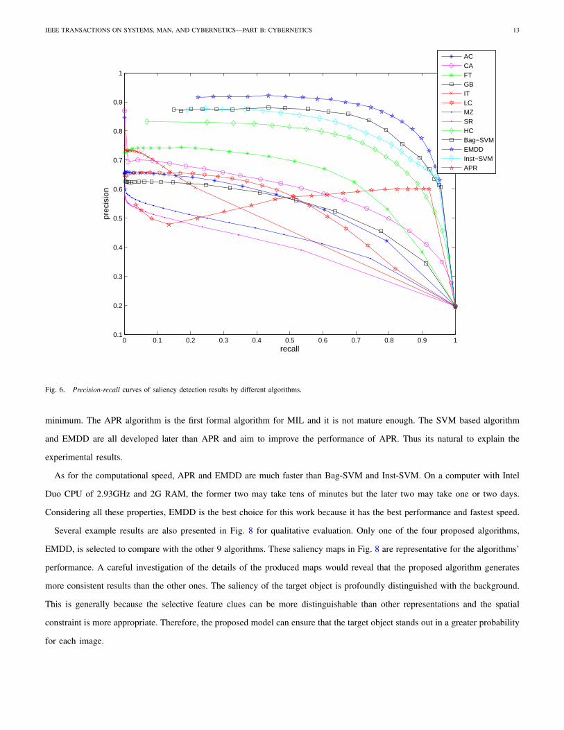
Fig. 7 and Fig. 8 illustrate the results. The precision-recall curves and the averaged precision, recall and F-measure bars

are obvious to show that three of the proposed algorithms, EMDD, Bag-SVM, and Inst-SVM outperforms the other 9 ones.

Achieving at the same precision value, the proposed algorithms can detect more salient regions; with the same recall value,

the proposed algorithms are more accurate. Only APR performs not very well, but its averaged recall and F-measure still

outperform most other 9 algorithms. This result is determined by the nature of APR learning algorithm. For APR, its learning

principle is simple and the learned model generalize poorly. It is achieved by increasing the size of an initially estimated

hyper-rectangle until every positive bag has at least one instance and every negative bag has no instance within it. In fact, there

is an implicit assumption that the feature data can be classified by an hyper-rectangle-like boundary. If the data distribution

follows the underlying principle, a good result can be obtained. Otherwise, if the positive and negative data interlace with each

other, a separating rectangle strictly dividing the data points into two sets is hard to find. Unfortunately in this work, feature

data are heavily interlaced. This makes the predicted results less accurate.

On the other hand, the SVM based algorithm projects the original data into another space by a kernel mapping. At the same

time, it maximizes the soft margin from the two types of positive and negative data. This makes the initially unclassified data

possible to be classified. The EMDD algorithm converts the multiple instance data to single instance data by removing all

but one point per bag in the E-step. This can not only reduce the computational time but also avoids getting caught in local


0 0.1 0.2 0.3 0.4 0.5 0.6 0.7 0.8 0.9 10.1

0.2

0.3

0.4

0.5

0.6

0.7

0.8

0.9

1

recall

prec

isio

n

ACCAFTGBITLCMZSRHCBag−SVMEMDDInst−SVMAPR

Fig. 6. Precision-recall curves of saliency detection results by different algorithms.

minimum. The APR algorithm is the first formal algorithm for MIL and it is not mature enough. The SVM based algorithm

and EMDD are all developed later than APR and aim to improve the performance of APR. Thus its natural to explain the

experimental results.

As for the computational speed, APR and EMDD are much faster than Bag-SVM and Inst-SVM. On a computer with Intel

Duo CPU of 2.93GHz and 2G RAM, the former two may take tens of minutes but the later two may take one or two days.

Considering all these properties, EMDD is the best choice for this work because it has the best performance and fastest speed.

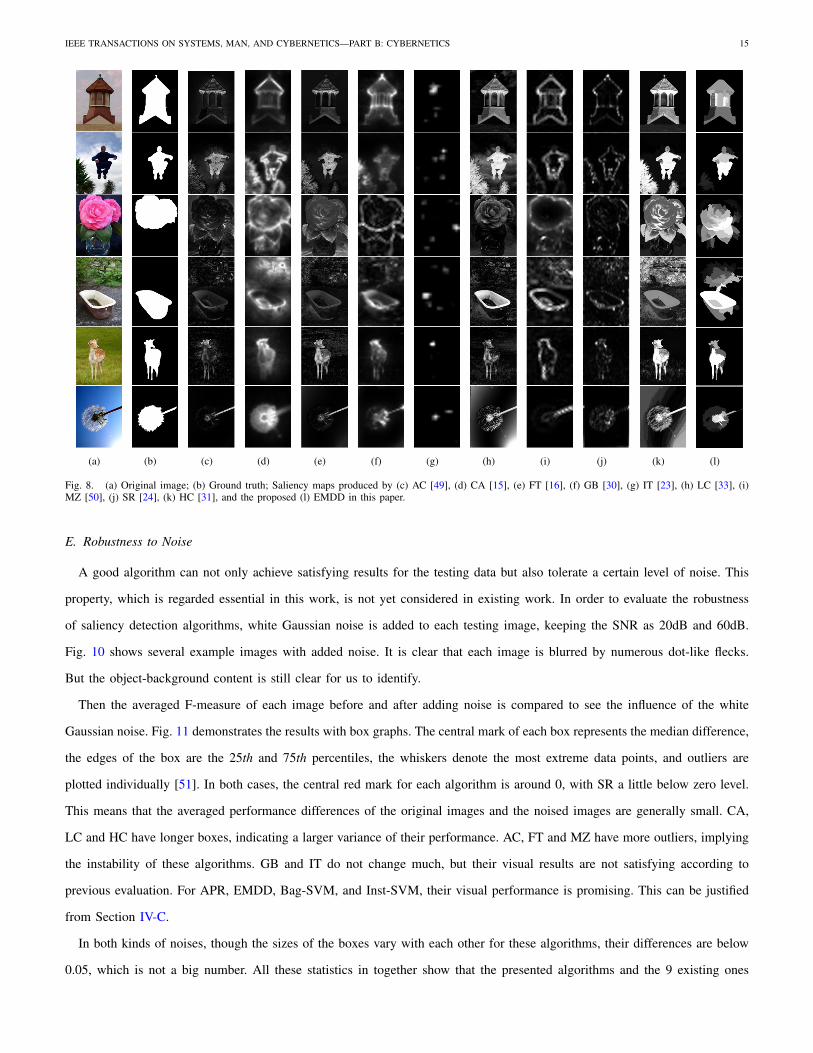
Several example results are also presented in Fig. 8 for qualitative evaluation. Only one of the four proposed algorithms,

EMDD, is selected to compare with the other 9 algorithms. These saliency maps in Fig. 8 are representative for the algorithms’

performance. A careful investigation of the details of the produced maps would reveal that the proposed algorithm generates

more consistent results than the other ones. The saliency of the target object is profoundly distinguished with the background.

This is generally because the selective feature clues can be more distinguishable than other representations and the spatial

constraint is more appropriate. Therefore, the proposed model can ensure that the target object stands out in a greater probability

for each image.


AC CA FT GB IT LC MZ SR HC APR EMDD Bag-SVM Inst-SVM0

0.1

0.2

0.3

0.4

0.5

0.6

0.7

0.8

0.9

precisionrecallF-measure

Fig. 7. Averaged precision, recall, and F-measure of saliency detection results by different algorithms.

D. Effects of Different Features

In this Section, effects of different features are evaluated to see whether its individual performance is better or its combination

is more suitable. Low-, high-level features and their combination are first tested separately. Then the mid-level feature, which

is actually a spatial prior constraint, is integrated. The final results are averaged on the four presented algorithms and shown in

Fig. 9. It is manifest that low- and high-level features performs not well individually. The mid-level feature can improve their

performance a lot. But the best performance is achieved by employing all these features. The results are reasonable to explain

because humans perceive the scene by an integrated feature cues. A specific type of feature can only reflect an incomplete

part of the information, while combining more image clues may make it more possible to understand the image content.

What deserves a further explanation of Fig. 9 is the fact that the detection results with the high-level feature perform worst

in the experiments. This does not to say the high-level feature is of less use. The reason is mainly that the high-level feature

is hard to extract and to utilize. Judd et al. [26] incorporated face detection results into their algorithm as a high-level feature.

This is lack of generality because not every image contains a face. Another option for employing a high-level feature is to

involve human interaction. But this is not practical for a large number of images. Therefore in this paper, a learned boundary

is adopted as a general high-level feature. The boundary feature is only effective to the bags with boundary pixels within them.

We believe the high-level feature is most important for saliency detection. But up to now, no perfect methodology is available

to extract this information and how to use the feature (generally or application specifically) is far less mature. The work in

this paper is just a meaningful attempt.


(a) (b) (c) (d) (e) (f) (g) (h) (i) (j) (k) (l)

Fig. 8. (a) Original image; (b) Ground truth; Saliency maps produced by (c) AC [49], (d) CA [15], (e) FT [16], (f) GB [30], (g) IT [23], (h) LC [33], (i)MZ [50], (j) SR [24], (k) HC [31], and the proposed (l) EMDD in this paper.

E. Robustness to Noise

A good algorithm can not only achieve satisfying results for the testing data but also tolerate a certain level of noise. This

property, which is regarded essential in this work, is not yet considered in existing work. In order to evaluate the robustness

of saliency detection algorithms, white Gaussian noise is added to each testing image, keeping the SNR as 20dB and 60dB.

Fig. 10 shows several example images with added noise. It is clear that each image is blurred by numerous dot-like flecks.

But the object-background content is still clear for us to identify.

Then the averaged F-measure of each image before and after adding noise is compared to see the influence of the white

Gaussian noise. Fig. 11 demonstrates the results with box graphs. The central mark of each box represents the median difference,

the edges of the box are the 25th and 75th percentiles, the whiskers denote the most extreme data points, and outliers are

plotted individually [51]. In both cases, the central red mark for each algorithm is around 0, with SR a little below zero level.

This means that the averaged performance differences of the original images and the noised images are generally small. CA,

LC and HC have longer boxes, indicating a larger variance of their performance. AC, FT and MZ have more outliers, implying

the instability of these algorithms. GB and IT do not change much, but their visual results are not satisfying according to

previous evaluation. For APR, EMDD, Bag-SVM, and Inst-SVM, their visual performance is promising. This can be justified

from Section IV-C.

In both kinds of noises, though the sizes of the boxes vary with each other for these algorithms, their differences are below

0.05, which is not a big number. All these statistics in together show that the presented algorithms and the 9 existing ones


0.2 0.3 0.4 0.5 0.6 0.7 0.8 0.9 1

0.2

0.3

0.4

0.5

0.6

0.7

0.8

0.9

recall

prec

isio

n

LowHighLowMidLowHighMidHighLowMidHigh

Fig. 9. Performance of saliency detection on different sets of features.

have a remarkable robustness to noises. But the proposed algorithms have a better visual performance.

V. IMAGE RETARGETING APPLICATION

A good saliency model enables many applications that effectively take the attention of human perception into account. In

order to comprehensively evaluate the proposed algorithms, the detected saliency map is further employed in an application

of seam carving.

Seam carving [52] [53] is an important technique for content based image resizing. A seam is defined as a connected path

of pixels going from the top (left) of an image to the bottom (right). By removing seams from an image, the image is resized

in the horizontal or the vertical dimension. A successful algorithm would ensure that the target object in the image should not

be disturbed.

In this work, seam carving is achieved by using an energy function defined on the pixels and removing minimum energy

paths from the image [52] [53]. The saliency map is evaluated in the context of defining the energy function. Then the seams

with the minimum energy paths are removed according a graph-cut framework. In the end, the image is resized to 75% width of

the original one and the results are judged subjectively. By this means, the effectiveness of saliency detection can be evaluated.

The HC algorithm [31], which has a comparable performance according to the precision-recall curves in Fig. 8, is chosen to


Fig. 10. Original images (first row) and its corresponding noisy images. Each image in the dataset is added with white Gaussian noise, keeping SNR as20dB (second row) and 60dB (third row).

be compared with the proposed EMDD algorithm. Fig. 12 shows the experimental results of seam carving. It is manifest that

the saliency maps by the proposed algorithm are better than the HC maps, with a higher and consistent saliency degree in the

target area. Therefore, the removed red seams in Fig. 12 (d) and Fig. 12 (g) are mainly from the background regions instead

of disturbing the target ones.

VI. DISCUSSION

In this Section, several issues related to the proposed algorithm are discussed. The first one is whether a Principle Component

Analysis (PCA) is needed to make the feature vector more compact. The second one is about multiple salient objects detection.

The third one is about the parameter selection of mean-shift segmentation algorithm. The fourth one analyzes the results on

images with rich-textures. In the end, some negative results are shown and analyzed.

A. PCA on Feature Vector

In the proposed algorithm, the feature vector is six dimensional, each component of which is respectively horizontal position,

vertical position, color contrast, texture contrast, scale contrast, and boundary identifier. Some argument may arise that a PCA


−0.25

−0.2

−0.15

−0.1

−0.05

0

0.05

0.1

0.15

0.2

0.25

AC CA FT GB IT LC MZ SR HC APR EMDD Bag-SVM Inst-SVM

(a)

−0.2

−0.15

−0.1

−0.05

0

0.05

0.1

0.15

0.2

AC CA FT GB IT LC MZ SR HC APR EMDD Bag−SVM Inst−SVM

(b)

Fig. 11. Performance comparison before and after adding noise to images. The statistics reflect the algorithms’ robustness to (a) 20dB noise; (b) 60dB noise.

analysis might be needed to make the feature vector more compact and optimal. To get the more appropriate representation, we

have conducted a set of comparative experiments. The original feature vector is re-represented on six orthogonal eigenvectors

by PCA. Then we reduce the dimensionality from six to one. Fig. 13 shows the precision-recall results averaged by the four

proposed algorithm on 800 testing images. From the curves, we can see that the six-dimensional PCA is close to the original

representation. The other reduced representation performs worse. The worst performance is the one-dimensional feature vector.

The reason behind this observation, we think, is that the original six features represent distinctive properties. There is no

redundancy among them. Consequently, the reduced dimensionality results in a less distinguishable ability. Based on these

experimental results, it is clear that the optimal feature representation is the original six-dimensional vector.


(a) (b) (c) (d) (e) (f) (g) (h)

Fig. 12. (a) Original image; (b) Ground truth; (c) Saliency map by HC [31], (d) its corresponding carved seams, and (e) resized image; (f) Saliency mapby the proposed algorithm EMDD, (g) its corresponding carved seams, and (h) resized image.

B. Multiple Object Detection

For an image, there may be more than one salient objects. Our processing dose not identify the number of salient objects

in the examined image, which we think is another different topic from what is discussed in this paper. We just detect the

salient areas for an input image, no matter it contains one or several objects. Therefore, if there are multiple salient objects, the

proposed algorithms can detect them, even when occlusions exist among objects. Many such examples abound in the employed

dataset. Fig. 14 demonstrates some typical examples.

C. Selection of Segmentation Parameter

The calculation of the proposed saliency detection algorithm is based on segmented regions. Therefore, the final results

are influenced by the segmentation outputs. Too small regions will lead to an inconsistent result and too large regions will

result in an enlarged salient area. A proper choice of the segmentation parameter is the insurance of a good saliency detection

result. There are three parameters for the employed mean-shift segmentation algorithm, spatial bandwidth, color bandwidth,

and minimum region. The default parameters are 7, 6.5, and 20, with which we find the saliency detection results are not

satisfying. Empirical experiments show that a combination of 15, 10.5, and 500 is more appropriate. Throughout the paper,

the segmentation is all conducted under this parameter set.

D. Results on Images with Rich-textures

For images with simple or no textures, the detected saliency results are mostly close to the ground truth labels. For images

with rich-textures, satisfying results can also be obtained because our training dataset contains images with different colors,


0 0.2 0.4 0.6 0.8 10.1

0.2

0.3

0.4

0.5

0.6

0.7

0.8

0.9

1

recall

prec

isio

n

Orig−6PCA−1PCA−2PCA−3PCA−4PCA−5PCA−6

Fig. 13. The performance comparison using feature representations of different dimensionalities.

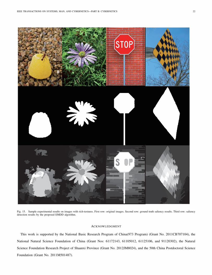
textures, and contents. The learned model can tackle a variety of testing images. Fig.15 illustrates some typical examples for

rich-textured images.

E. Analysis of Negative Results

In this Section, several negative experimental results are demonstrated and analyzed. It can be seen from Fig. 16 that

the obtained results by the proposed algorithm are not satisfying compared with the ground truth saliency results. We think

there are three reasons for this problem. First, the segmentation results are not consistent with the human perception. Since the

proposed algorithm calculates saliency on regions, which are acquired through segmentation, the segmentation results are highly

correlated to the saliency calculation. Unfortunately, the state-of-the-art for segmentation algorithms has not reached a level

comparable with human perception. This will result in a segmented object splitting into several parts. The first column of Fig.

16 is a typical example of this case. The wheel in the image is segmented as several parts, leading to an inconsistent detection

result. Second, without appropriate higher level clues, the detected saliency can hardly reflect human’s experience. This can

be illustrated in the second column of Fig. 16. People will generally pay more attention to the object held in hand, rather than

the hand itself. But the computer cannot handle this situation. Though the boundary clue is incorporated in our processing, it


Fig. 14. Illustrative detection of multiple salient objects. First column: original images. Second column: ground truth saliency results. Third column: saliencydetection results by the proposed EMDD algorithm.

is far from perfect to reflect a complete human experience. Third, the content of the image is sometimes ambiguous itself. In

the third column of Fig. 16, it is difficult to tell which of the badge and the picture frame is more salient.

VII. CONCLUSION

In this paper, a supervised framework for saliency detection has been presented. The framework combines a set of low-, mid-,

and high-level features to predict the possibilities of each region being salient. The approach it takes is multiple instance learning

and four implementations of MIL are demonstrated. To validate the effectiveness and robustness, 9 algorithms representing the

sate-of-the-art are employed to be compared with the proposed one. Experiments on a set of 1,000 images show that the MIL

based one outperforms the others. An application of seam carving is also involved to exemplify the usefulness of the proposed

framework.

There are several remaining issues for further investigation. The first one is how to extract more effective high-level features

to be effectively incorporated into the detection framework. We believe that this might be the key point for tremendously

improving the state-of-the-art. The second one is how to apply the saliency detection technique to specific applications.


Fig. 15. Sample experimental results on images with rich-textures. First row: original images. Second row: ground truth saliency results. Third row: saliencydetection results by the proposed EMDD algorithm.

ACKNOWLEDGMENT

This work is supported by the National Basic Research Program of China(973 Program) (Grant No. 2011CB707104), the

National Natural Science Foundation of China (Grant Nos: 61172143, 61105012, 61125106, and 91120302), the Natural

Science Foundation Research Project of Shaanxi Province (Grant No. 2012JM8024), and the 50th China Postdoctoral Science

Foundation (Grant No. 2011M501487).


Fig. 16. Illustration of several negative results.

REFERENCES

[1] W. James, The Principles of Psychology. New York: Henry Holt, 1890, vol. 1.

[2] Y. Yu, G. K. I. Mann, and R. G. Gosine, “An object-based visual attention model for robotic applications,” IEEE Trans. Syst., Man, Cybern. B, Cybern.,

vol. 40, no. 5, pp. 1398–1412, 2010.

[3] K. Huang, D. Tao, Y. Y. Tang, X. Li, and T. Tan, “Biologically inspired features for scene classification in video surveillance,” IEEE Trans. Syst., Man,

Cybern. B, Cybern., vol. 41, no. 1, pp. 307–313, 2011.

[4] Y. Huang, K. Huang, D. Tao, T. Tan, and X. Li, “Enhanced biologically inspired model for object recognition,” IEEE Trans. Syst., Man, Cybern. B,

Cybern., vol. 41, no. 6, pp. 1668–1680, 2011.

[5] A. Oikonomopoulos, I. Patras, and M. Pantic, “Spatiotemporal salient points for visual recognition of human actions,” IEEE Trans. Syst., Man, Cybern.

B, Cybern., vol. 36, no. 3, pp. 710–719, 2006.

[6] D. Walther, L. Itti, M. Riesenhuber, T. Poggio, and C. Koch, “Attentional selection for object recognition a gentle way,” in Biologically Motivated

Computer Vision, 2002, pp. 472–479.

[7] J. Han, K. N. Ngan, M. Li, and H. Zhang, “Unsupervised extraction of visual attention objects in color images,” IEEE Trans. Circuits Syst. Video Techn.,

vol. 16, no. 1, pp. 141–145, 2006.

[8] B. C. Ko and J.-Y. Nam, “Object-of-interest image segmentation based on human attention and semantic region clustering,” Journal of Optical Society

of America A, vol. 23, no. 10, pp. 2462–2470, 2006.

[9] Y.-S. Wang, C.-L. Tai, O. Sorkine, and T.-Y. Lee, “Optimized scale-and-stretch for image resizing,” ACM Trans. Graph., vol. 27, no. 5, pp. 1–8, 2008.


[10] T. Chen, M.-M. Cheng, P. Tan, A. Shamir, and S.-M. Hu, “Sketch2photo: internet image montage,” ACM Trans. Graph., vol. 28, no. 5, pp. 1–10, 2009.

[11] L. Chen, X. Xie, X. Fan, W.-Y. Ma, H.-J. Zhang, and H. Zhou, “A visual attention model for adapting images on small displays,” Microsoft Research,

Redmond, MA, Tech. Rep. MSR-TR-2002-125, 2002.

[12] L. Itti, “Models of bottom-up and top-down visual attention,” Ph.D. dissertation, California Institute of Technology, 2000. [Online]. Available:

http://ilab.usc.edu/publications/2000.html

[13] X. Gao, N. Liu, W. Lu, D. Tao, and X. Li, “Spatio-temporal salience based video quality assessment,” in IEEE Int’l Conf. Systems Man and Cybernetics,

2010, pp. 1501–1505.

[14] X. Li, S. Lin, S. Yan, and D. Xu, “Discriminant locally linear embedding with high-order tensor data,” IEEE Trans. Syst., Man, Cybern. B, Cybern.,

vol. 38, no. 2, pp. 342–352, 2008.

[15] S. Goferman, L. Zelnik-Manor, , and A. Tal, “Context-aware saliency detection,” in IEEE Int’l Conf. Computer Vision and Pattern Recognition, 2010.

[16] R. Achanta, S. Hemami, F. Estrada, and S. Susstrunk, “Frequency-tuned salient region detection,” in IEEE Int’l Conf. Computer Vision and Pattern

Recognition, 2009.

[17] K.-Y. Chang, T.-L. Liu, and S.-H. Lai, “From co-saliency to co-segmentation: an efficient and fully unsupervised energy minimization model,” in IEEE

Int’l Conf. Computer Vision and Pattern Recognition, 2011.

[18] J. M. Wolfe and T. S. Horowitz, “What attributes guide the deployment of visual attention and how do they do it,” Nature Reviews Neuroscience, vol. 5,

pp. 1–7, 2004.

[19] A. Treisman and G. Gelade, “A featrue-integration theory of attention,” Cognitive Psychology, vol. 12, pp. 97–136, 1980.

[20] R. Desimone and J. Duncan, “Neural mechanisms of selective visual attention,” Annual Review of Neuroscience, vol. 18, pp. 193–222, 1995.

[21] T. G. Dietterich, R. H. Lathrop, and T. Lozano-Perez, “Solving the multiple instance problem with axis-parallel rectangles,” Artificial Intelligence, vol. 89,

no. 1-2, pp. 31–71, 1997.

[22] C. Koch and S. Ullman, “Shifts in selective visual attention: towards the underlying neural circuitry,” Human Neurobiology, vol. 4, no. 4, pp. 97–136,

1985.

[23] L. Itti, C. Koch, and E. Niebur, “A model of saliency-based visual attention for rapid scene analysis,” IEEE Trans. Pattern Anal. Mach. Intell., vol. 21,

no. 11, pp. 1254–1259, 1998.

[24] X. Hou and L. Zhang, “Saliency detection: A spectral residual approach,” in IEEE Int’l Conf. Computer Vision and Pattern Recognition, 2007, pp. 1–8.

[25] T. Liu, J. Sun, N. Zheng, X. Tang, and H.-Y. Shum, “Learning to detect a salient object,” in IEEE Int’l Conf. Computer Vision and Pattern Recognition,

2007.

[26] T. Judd, K. A. Ehinger, F. Durand, and A. Torralba, “Learning to predict where humans look,” in Int’l Conf. Computer Vision, 2009, pp. 2106–2113.

[27] Z. Wang and B. Li, “A two-stage approach to saliency detection in images,” in IEEE Int’l Conf. Acoustics, Speech and Signal Processing, 2008, pp.

965– 968.

[28] A. Radhakrishna and S. Sabine, “Saliency detection using maximum symmetric surround,” in IEEE Int’l Conf. Image Processing, 2010.

[29] L. Zhang, M. H. Tong, T. K. Marks, H. Shan, and G. W. Cottrell, “Sun: A bayesian framework for saliency using natural statistics,” Journal of Vison,

vol. 8, no. 7, pp. 1–20, 2008.

[30] J. Harel and P. P. C. Koch, “Graph-based visual saliency,” in Advances in Neural Information Processing Systems, 2006, pp. 545–552.

[31] M.-M. Cheng, G.-X. Zhang, N. J. Mitra, X. Huang, and S.-M. Hu, “Global contrast based salient region detection,” in IEEE Int’l Conf. Computer Vision

and Pattern Recognition, 2011.

[32] M. Wang, J. Konrad, P. Ishwar, K. Jing, and H. A. Rowley, “Image saliency: from intrinsic to extrinsic context,” in IEEE Int’l Conf. Computer Vision

and Pattern Recognition, 2011.

[33] Y. Zhai and M. Shah, “Visual attention detection in video sequences using spatiotemporal cues,” in ACM Multimedia, 2006.

[34] T. Liu, Z. Yuan, J. Sun, J. Wang, N. Zheng, X. Tang, and H.-Y. Shum, “Learning to detect a salient object,” IEEE Trans. Pattern Anal. Mach. Intell.,

vol. 33, no. 2, pp. 353–367, 2011.

[35] S. Andrews, I. Tsochantaridis, and T. Hofmann, “Support vector machines for multiple-instance learning,” in Advances in Neural Information Processing

Systems, 2002, pp. 561–568.

[36] J. Wang and J.-D. Zucker, “Solving the multiple-instance problem: A lazy learning approach,” in Int’l Conf. Machine Learning, 2000, pp. 1119–1126.

[37] R. A. Amar, D. R. Dooly, S. A. Goldman, and Q. Zhang, “Multiple-instance learning of real-valued data,” in Int’l Conf. Machine Learning, 2001, pp.

3–10.


[38] P. A. Viola, J. C. Platt, and C. Zhang, “Multiple instance boosting for object detection,” in Advances in Neural Information Processing Systems, 2005.

[39] B. Babenko, M.-H. Yang, and S. Belongie, “Robust object tracking with online multiple instance learning,” IEEE Trans. Pattern Anal. Mach. Intell.,

vol. 33, no. 8, pp. 1619–1632, 2011.

[40] Q. Zhang and S. A. Goldman, “Em-dd: An improved multiple-instance learning technique,” in Advances in Neural Information Processing Systems,

2001, pp. 1073–1080.

[41] O. Maron and T. Lozano-Perez, “A framework for multiple-instance learning,” in Advances in Neural Information Processing Systems, 1997.

[42] O. Maron and A. L. Ratan, “Multiple-instance learning for natural scene classification,” in Int’l Conf. Machine Learning, 1998, pp. 341–349.

[43] D. Comaniciu and P. Meer, “Mean shift: A robust approach toward feature space analysis,” IEEE Trans. Pattern Anal. Mach. Intell., vol. 24, no. 5, pp.

603–619, 2002.

[44] J. Malik, S. Belongie, T. K. Leung, and J. Shi, “Contour and texture analysis for image segmentation,” International Journal of Computer Vision, vol. 43,

no. 1, pp. 7–27, 2001.

[45] J. Han, K. N. Ngan, M. Li, and H. Zhang, “Unsupervised extraction of visual attention objects in color images,” IEEE Trans. Circuits Syst. Video Techn.,

vol. 16, no. 1, pp. 141–145, 2006.

[46] D. R. Martin, C. Fowlkes, and J. Malik, “Learning to detect natural image boundaries using local brightness, color, and texture cues,” IEEE Trans.

Pattern Anal. Mach. Intell., vol. 26, no. 5, pp. 530–549, 2004.

[47] D. L. Olson and D. Delen, Advanced Data Mining Techniques. Springer, March 4, 2008.

[48] [Online]. Available: http://en.wikipedia.org/wiki/Precision and recall

[49] R. Achanta, F. J. Estrada, P. Wils, and S. Susstrunk, “Salient region detection and segmentation,” in Computer Vision Systems, 2008, pp. 66–75.

[50] Y.-F. Ma and H. Zhang, “Contrast-based image attention analysis by using fuzzy growing,” in ACM Multimedia, 2003, pp. 374–381.

[51] [Online]. Available: www.mathworks.cn/help/toolbox/stats/boxplot.html

[52] S. Avidan and A. Shamir, “Seam carving for content-aware image resizing,” ACM Transactions on Graphics, vol. 26, no. 3, p. 10, 2007.

[53] M. Rubinstein, A. Shamir, and S. Avidan, “Improved seam carving for video retargeting,” ACM Transactions on Graphics, vol. 27, no. 3, 2008.

Qi Wang received the B.E. degree in automation and Ph.D. degree in pattern recognition and intelligent system from the University

of Science and Technology of China, Hefei, China, in 2005 and 2010 respectively. He is currently a postdoctoral researcher with

the Center for Optical Imagery Analysis and Learning, State Key Laboratory of Transient Optics and Photonics, Xi’an Institute of

Optics and Precision Mechanics, Chinese Academy of Sciences, Xi’an, China. His research interests include computer vision and

pattern recognition.

Yuan Yuan (M’05-SM’09) is a researcher (full professor) with Chinese Academy of Sciences, and her main research interests include Visual Information

Processing and Image/Video Content Analysis.

26

Pingkun Yan (S’04-M’06-SM’10) received the B.Eng. degree in electronics engineering and information science from the University

of Science and Technology of China, Hefei, China and the Ph.D. degree in electrical and computer engineering from the National

University of Singapore, Singapore. He is a full professor with the Center for OPTical IMagery Analysis and Learning (OPTIMAL),

State Key Laboratory of Transient Optics and Photonics, Xi’an Institute of Optics and Precision Mechanics, Chinese Academy of

Sciences, Xi’an 710119, Shaanxi, P. R. China. His research interests include computer vision, pattern recognition, machine learning,

and their applications in medical imaging.

Xuelong Li (M’02-SM’07-F’12) is a full professor with the Center for OPTical IMagery Analysis and Learning (OPTIMAL), State Key Laboratory of

Transient Optics and Photonics, Xi’an Institute of Optics and Precision Mechanics, Chinese Academy of Sciences, Xi’an 710119, Shaanxi, P. R. China.

Documents

IEEE TRANSACTIONS ON SYSTEMS, MAN, AND CYBERNETICS… Saliency... · IEEE TRANSACTIONS ON SYSTEMS, MAN, AND CYBERNETICS—PART B: CYBERNETICS 1 Saliency Detection by Multiple Instance