1098 IEEE TRANSACTIONS ON SYSTEMS, MAN, AND CYBERNETICS ...syllabus.cs.manchester.ac.uk/pgt/2019/COMP61021/... · 1098 IEEE TRANSACTIONS ON SYSTEMS, MAN, AND CYBERNETICS—PART B:

1098 IEEE TRANSACTIONS ON SYSTEMS, MAN, AND CYBERNETICS—PART B: CYBERNETICS, VOL. 35, NO. 6, DECEMBER 2005

Supervised Nonlinear Dimensionality Reductionfor Visualization and Classification

Xin Geng, De-Chuan Zhan, and Zhi-Hua Zhou, Member, IEEE

Abstract—When performing visualization and classification,people often confront the problem of dimensionality reduction.Isomap is one of the most promising nonlinear dimensionalityreduction techniques. However, when Isomap is applied toreal-world data, it shows some limitations, such as being sensitiveto noise. In this paper, an improved version of Isomap, namelyS-Isomap, is proposed. S-Isomap utilizes class information toguide the procedure of nonlinear dimensionality reduction. Sucha kind of procedure is called supervised nonlinear dimensionalityreduction. In S-Isomap, the neighborhood graph of the input datais constructed according to a certain kind of dissimilarity betweendata points, which is specially designed to integrate the classinformation. The dissimilarity has several good properties whichhelp to discover the true neighborhood of the data and, thus,makes S-Isomap a robust technique for both visualization andclassification, especially for real-world problems. In the visualiza-tion experiments, S-Isomap is compared with Isomap, LLE, andWeightedIso. The results show that S-Isomap performs the best.In the classification experiments, S-Isomap is used as a preprocessof classification and compared with Isomap, WeightedIso, as wellas some other well-established classification methods, includingthe K-nearest neighbor classifier, BP neural network, J4.8 decisiontree, and SVM. The results reveal that S-Isomap excels comparedto Isomap and WeightedIso in classification, and it is highlycompetitive with those well-known classification methods.

Index Terms—Classification, dimensionality reduction, manifoldlearning, supervised learning, visualization.

I. INTRODUCTION

WITH the wide usage of information technology in al-most all aspects of daily lives, huge amounts of data,

such as climate patterns, gene distributions, and commercialrecords, have been accumulated in various databases and datawarehouses. Most of these data have many attributes, i.e., theyare distributed in high-dimensional spaces. People workingwith them regularly confront the problem of dimensionalityreduction, which is a procedure of finding intrinsic low-dimen-sional structures hidden in the high-dimensional observations.This may be a crucial step for the tasks of data visualization orclassification.

Dimensionality reduction can be performed by keeping onlythe most important dimensions, i.e., the ones that hold the mostuseful information for the task at hand, or by projecting the orig-inal data into a lower dimensional space that is most expressive

Manuscript received February 13, 2004; revised June 10, 2004. This workwas supported by the National Outstanding Youth Foundation of China underGrant 60325207. This paper was recommended by Associate Editor D. Nauck.

The authors are with the National Laboratory for Novel Software Technology,Nanjing University, Nanjing 210093, China (e-mail: [email protected];[email protected]; [email protected]).

Digital Object Identifier 10.1109/TSMCB.2005.850151

for the task. For visualization, the goal of dimensionality re-duction is to map a set of observations into a [two-dimensional(2-D) or three-dimensional (3-D)] space that preserves, as muchas possible, the intrinsic structure. For classification, the goal isto map the input data into a feature space in which the membersfrom different classes are clearly separated.

Many approaches have been proposed for dimensionalityreduction, such as the well-known methods of principal com-ponent analysis (PCA) [5], independent component analysis(ICA) [2], and multidimensional scaling (MDS) [3]. In PCA,the main idea is to find the projection that restores the largestpossible variance in the original data. ICA is similar to PCAexcept that the components are designed to be independent.Finally, in MDS, efforts are taken to find the low-dimensionalembeddings that best preserve the pair wise distances betweenthe original data points. All of these methods are easy to imple-ment. At the same time, their optimizations are well understoodand efficient. Because of these advantages, they have beenwidely used in visualization and classification. Unfortunately,they have a common inherent limitation: They are all linearmethods while the distributions of most real-world data arenonlinear.

Recently, two novel methods have been proposed to tacklethe nonlinear dimensionality reduction problem, namely Isomap[13] and LLE [9]. Both of these methods attempt to preserve aswell as possible the local neighborhood of each object whiletrying to obtain highly nonlinear embeddings. So they are cat-egorized as a new kind of dimensionality reduction techniquescalled local embeddings [16]. The central idea of local embed-dings is using the locally linear fitting to solve the globally non-linear problems, which is based on the assumption that datalying on a nonlinear manifold can be viewed as linear in localareas. Both Isomap and LLE have been used in visualization [9],[11], [13], [16] and classification [11], [16]. Encouraging resultshave been reported when the test data contain little noise and arewell sampled, but, as can been seen in the following sections ofthis paper, they are not so powerful when confronted with noisydata, which is often the case for real-world problems. In thispaper, a robust method based on the idea of Isomap, namelyS-Isomap, is proposed to deal with such situation. Unlike theunsupervised learning scheme of Isomap, S-Isomap follows thesupervised learning scheme, i.e., it uses the class labels of theinput data to guide the manifold learning.

The rest of this paper is organized as follows. In Section II,Isomap and the usage of it in visualization and classification arebriefly introduced. In Section III, S-Isomap is proposed, and theusage of it in visualization and classification is also discussed.In Section IV, experiments are reported. Finally, in Section V,

1083-4419/$20.00 © 2005 IEEE

GENG et al.: SUPERVISED NONLINEAR DIMENSIONALITY REDUCTION 1099

conclusions are drawn and several issues for the future work areindicated.

II. ISOMAP FOR VISUALIZATION AND CLASSIFICATION

For data lying on a nonlinear manifold, the “true distance”between two data points is the geodesic distance on the mani-fold, i.e., the distance along the surface of the manifold, ratherthan the straight-line Euclidean distance. The main purpose ofIsomap is to find the intrinsic geometry of the data, as capturedin the geodesic manifold distances between all pairs of datapoints. The approximation of geodesic distance is divided intotwo cases. In case of neighboring points, Euclidean distance inthe input space provides a good approximation to geodesic dis-tance. In case of faraway points, geodesic distance can be ap-proximated by adding up a sequence of “short hops” betweenneighboring points. Isomap shares some advantages with PCA,LDA, and MDS, such as computational efficiency and asymp-totic convergence guarantees, but with more flexibility to learn abroad class of nonlinear manifolds. The Isomap algorithm takesas input the distances between all pairs and from

data points in the high-dimensional input space . The al-gorithm outputs coordinate vectors in a -dimensional Eu-clidean space that best represent the intrinsic geometry of thedata. The detailed steps of Isomap are listed as follows.

Step 1) Construct neighborhood graph: Define the graphover all data points by connecting points andif they are closer than a certain distance , or if isone of the -nearest neighbors ( -NN) of . Setedge lengths equal to .

Step 2) Compute shortest paths: Initializeif and are linked by an edge;

otherwise. Then, for eachvalue of , in turn, replace all en-tries by

. The matrix of final valueswill contain the shortest path dis-

tances between all pairs of points in (this proce-dure is known as Floyd’s algorithm).

Step 3) Construct -dimensional embedding: Let bethe th eigenvalue (in decreasing order) of thematrix (The operator is defined by

, where is the matrix ofsquared distances , and is the“centering matrix” is theKronecker delta function [7]), and be the thcomponent of the th eigenvector. Then set the thcomponent of the -dimensional coordinate vector

equal to (This is actually a procedureof applying classical MDS to the matrix of graphdistances ).

Note that the only free parameter of Isomap, or , appearsin Step 1). In this paper, only the parameter is used in Isomap.

Isomap can be easily applied to visualization. In this case, 2-Dor 3-D embeddings of higher dimensional data are constructedusing Isomap and then depicted in a single global coordinatesystem. Isomap’s global coordinates provide a simple way toanalyze and manipulate high-dimensional observations in terms

of their intrinsic nonlinear degrees of freedom. Isomap has beensuccessfully used to detect the true underlying factors of somehigh-dimensional data sets, such as synthetic face images, handgesture images, and handwritten digits [13]. However, as canbe seen in the following sections, when the input data are morecomplex and noisy, such as a set of face images captured bya web camera, Isomap often fails to nicely visualize them. Thereason is that the local neighborhood structure determined in thefirst step of Isomap is critically distorted by the noise.

As for the classification tasks, Isomap can be viewed asa preprocess. When the dimensionality of the input data isrelatively high, most classification methods, such as -NNclassifier [4], [6], will suffer from the curse of dimensionalityand get highly biased estimates. Fortunately, high-dimensionaldata often represent phenomena that are intrinsically lowdimensional. Thus, the problem of high-dimensional data clas-sification can be solved by first mapping the original data intoa lower dimensional space by Isomap (which can be viewedas a preprocess) and then applying -NN classification to theimages. Since the mapping function is not explicitly given byIsomap, it should be learned by some nonlinear interpolationtechniques, such as generalized regression networks [17].Suppose that the data in are mapped into byIsomap. The mapping function can be learnedby generalized regression networks, using the correspondingdata pairs in and as the training set. A given query isfirst mapped into to get its lower dimensional image .Then, its class label is given as the most frequent one occurringin the neighbors of in . Unfortunately, this schemeseems not to work very well compared with those widely usedclassification methods (according to the experiments in thispaper), such as BP network [10], decision tree [8], and SVM[14], [15]. There may be two reasons. First, the real-world dataare often noisy, which can weaken the mapping procedure ofIsomap. Second, the goal of the mapping in classification isdifferent from that in visualization. In visualization, the goal isto faithfully preserve the intrinsic structure as well as possible,while in classification, the goal is to transform the originaldata into a feature space that can make classification easier, bystretching or constricting the original metric if necessary. Bothreasons indicate that some modification should be made onIsomap for the tasks of classification.

III. SUPERVISED ISOMAP: S-ISOMAP

In some visualization tasks, data are from multiple classesand the class labels are known. In classification tasks, the classlabels of all training data must be known. The information pro-vided by these class labels may be used to guide the procedure ofdimensionality reduction. This can be called supervised dimen-sionality reduction, in contrast to the unsupervised scheme ofmost dimensionality reduction methods. Some preliminary ef-forts have already been taken toward supervised dimensionalityreduction, such as the WeightedIso method [16], which changesthe first step of Isomap by rescaling the Euclidean distance be-tween two data points with a constant factor if theirclass labels are the same. The basic idea behind WeightedIsois to make the two points closer to each other in the feature


Fig. 1. Typical plot of D(x ;x ) as a function of d (x ;x )=�.

space if they belong to the same class. It is believed that thiscan make classification in the feature space easier. However,WeightedIso is not suitable for visualization because it force-fully distorts the original structure of the input data no matterwhether there is noise in the data or not and how much noiseis in the data. Even in classification, the factor must be verycarefully tuned to get a satisfying result (this has been well ex-perienced in the following experiments). To make the algorithmmore robust for both visualization and classification, a more so-phisticated method is proposed in this section.

Suppose the given observations are ,where and is the class label of . Define the dis-similarity between two points and as

(1)

where denotes the Euclidean distance between and. A typical plot of as a function of

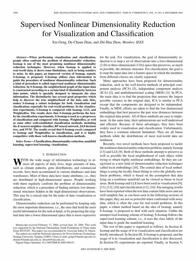
is shown in Fig. 1. Since the Euclidean distance is inthe exponent, the parameter is used to prevent toincrease too fast when is relatively large. Thus, thevalue of should depend on the “density” of the data set. Usu-ally, is set to be the average Euclidean distance between allpairs of data points. The parameter gives a certain chance tothe points in different classes to be “more similar,” i.e., to have asmaller value of dissimilarity, than those in the same class. Fora better understanding of , it may be helpful to look at Fig. 2,which is the typical plot of defined in (2)

(2)

In Fig. 2, the dissimilarity between two points is equal to orlarger than 1 if their class labels are different and is less than1 if otherwise. Thus, the interclass dissimilarity is definitelylarger than the intraclass dissimilarity, which is a very goodproperty for classification. However, this can also make the al-gorithm apt to overfit the training set. Moreover, this can oftenmake the neighborhood graph of the input data disconnected,which is a situation that Isomap cannot handle. So is used tolose the restriction and give the intraclass dissimilarity a certain

Fig. 2. Typical plot of D (x ;x ) as a function of d (x ;x )=�.

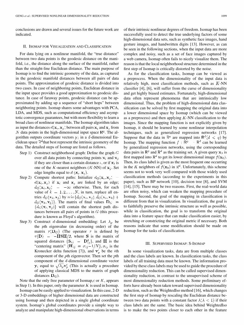
Fig. 3. Typical plot of WD(x ;x ) as a function of d(x ;x ).

probability to exceed the interclass dissimilarity. The value ofshould be greater than 0 and less than the value that makes

the two curves tangent (when the two curves are tangent to eachother, is about 0.65 and the value of at whichthe two curves touch is about 0.38). It is worth mentioning thatthe function of can also be achieved through subtracting aconstant from the squared dissimilarity , it does notmatter much.

As a point of comparison, the typical plot of the dis-similarity used in WeightedIso, namely , asa function of , is shown in Fig. 3 .When ; otherwise,

. Thus, the intraclass dissimi-larity is linearly reduced while the interclass dissimilarity keepsunchanged. This does offer some help to classification, but withlimited ability to control the noise in the data. In detail, therange of , whether or , is .This means the noise, theoretically speaking, can change theoriginal dissimilarity to any value in . Consequently, solong as the noise is strong enough, the neighborhood relation-ship among the data points can be completely destroyed.

As for the dissimilarity , its properties and the cor-responding advantages can be summarized as follows.

Property 1: When the Euclidean distance is equal, the inter-class dissimilarity is larger than the intraclass dissimilarity. Thisis similar to and makes suitable for clas-sification tasks.

Property 2: The interclass dissimilarity is equal to or largerthan while the intraclass dissimilarity is less than 1. Thus,


no matter how strong the noise is, the interclass and intraclassdissimilarity can be controlled in certain ranges, respectively.This makes suitable to apply to noisy data.

Property 3: Each dissimilarity function is monotone in-creasing with respect to the Euclidean distance. This ensuresthat the main geometric structure of the original data set, whichis embodied by the Euclidean distances among data points, canbe preserved.

Property 4: With the increase of the Euclidean distance, theinterclass dissimilarity increases faster while the intraclass dis-similarity increases slower. This endows with certainability to “recognize” noise in the data. On the one hand, the in-traclass distance is usually small. So, the larger it is, the morepossible the noise exists, and the slower increases. Onthe other hand, the interclass distance is usually large. So, thesmaller it is, the more possible the noise exists, and the slower

decreases. Both aspects indicate that cangradually strengthen the power of noise suppression with the in-crease of noise-existing possibility.

Because of these good properties, the dissimilaritycan be used in the procedure of Isomap to address the robustnessproblem in visualization and classification. Since in-tegrates the class information, this algorithm is called super-vised Isomap, denoted by S-Isomap. There are also three stepsin S-Isomap. In the first step, neighborhood graph of the inputdata is constructed according to the dissimilarity between datapoints. The neighborhood can be defined as the most sim-ilar points or the points whose dissimilarity is less than a cer-tain value . In this paper, the neighborhood is defined as themost similar points. If two points and are neighbors, thenconnect them with an edge and assign to the edge asa weight. The second step is similar to that of Isomap, but theshortest path between each pair of points is computed accordingto the weight of the edge rather than the Euclidean distance be-tween the points. However, for convenience of discussion, theword “distance” is still used to indicate the sum of the weightsalong the shortest path. Finally, the third step of S-Isomap is thesame as that of Isomap.

A. S-Isomap for Visualization

For visualization, the goal is to map the original data set intoa (2-D or 3-D) space that preserves as much as possible the in-trinsic structure. Isomap can do this well when the input dataare well sampled and have little noise. As for noisy data, whichis common in real world, Isomap often fails to nicely visualizethem. In this situation, the class labels of the data, if known, canbe used to relieve the negative effect of noise. It is well knownthat points belonging to the same class are often closer to eachother than those belonging to different classes. Under this as-sumption, S-Isomap can be used to recover the true manifoldof the noisy data. In the first step of S-Isomap, pullspoints belonging to the same class closer and propels those be-longing to different classes further away (Property 1). Recallthat has certain ability to “recognize” noise (Property4), so when the data are noisy, this procedure can counteract theeffect of noise and help to find the true neighborhood, and whenthe data are not noisy, this procedure hardly affects the neighbor-hood constructing. In both cases, ensures to preserve

the intrinsic structure of the data set (Property 3) and boundsthe effect of noise in the data (Property 2). Thus, S-Isomap issuitable to visualize the real-world data, whether noisy or not.

B. S-Isomap for Classification

For classification, the goal is to map the data into a featurespace in which the members from different classes are clearlyseparated. S-Isomap can map the data into such a space wherepoints belonging to the same class are close to each other whilethose belonging to different classes are far away from each other(Property 1). At the same time, the main structure of the originaldata can be preserved (Property 3). It is obvious that performingclassification in such a space is much easier. When the data arenoisy, S-Isomap can detect the existence of noise (Property 4)and limit the effect of noisy (Property 2). Thus, S-Isomap canbe used to design a robust classification method for real-worlddata. The procedure is similar to that of using Isomap in classi-fication, which has been described in Section II. To summarize,the classification has three steps as follows.

1) Map the data into a lower dimensional space usingS-Isomap.

2) Construct generalized regression network to approximatethe mapping.

3) Map the given query using the generalized regression net-work and then predict its class label using K-NN.

IV. EXPERIMENTS

A. Visualization

1) Methodology: In many previous works on visualization,the results are mainly compared through examining the figuresto point out which “looks” better. To compare the results moreimpersonally, some numerical criteria should be designed.When the distances between all pairs of data points are simul-taneously changed by a linear transformation, the relationshipof the points will not change, in other words, the intrinsicstructure will not change. Recall that the goal of visualizationis to faithfully represent the intrinsic structure of the input data.Thus, the correlation coefficient between the distance vectors,i.e., the vectors that comprises the distances between all pairs ofpoints, of the true structure and that of the recovered structureprovides a good measurement of the validity of the visualizationprocedure. Suppose the distance vector of the true structureis and that of the recovered structure is , then thecorrelation coefficient between and is computed by

(3)

where is the average operator, represents the el-ement-by-element product, and is the standard deviation ofthe vector’s elements. The larger the value of , thebetter the performance of the visualization is.

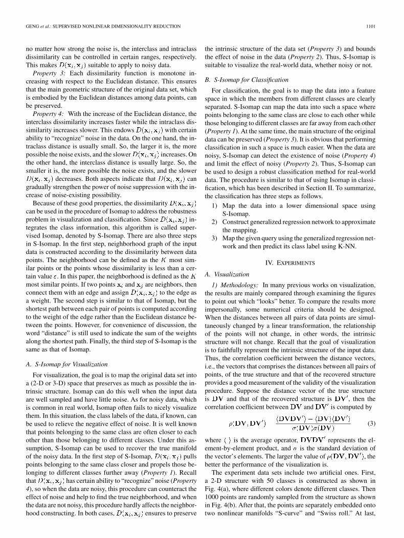
The experiment data sets include two artificial ones. First,a 2-D structure with 50 classes is constructed as shown inFig. 4(a), where different colors denote different classes. Then1000 points are randomly sampled from the structure as shownin Fig. 4(b). After that, the points are separately embedded ontotwo nonlinear manifolds “S-curve” and “Swiss roll.” At last,


Fig. 4. Artificial data sets. (a) Class structure. (b) Random samples. (c) Samples imbedded on S-curve. (d) Samples imbedded on Swiss roll.

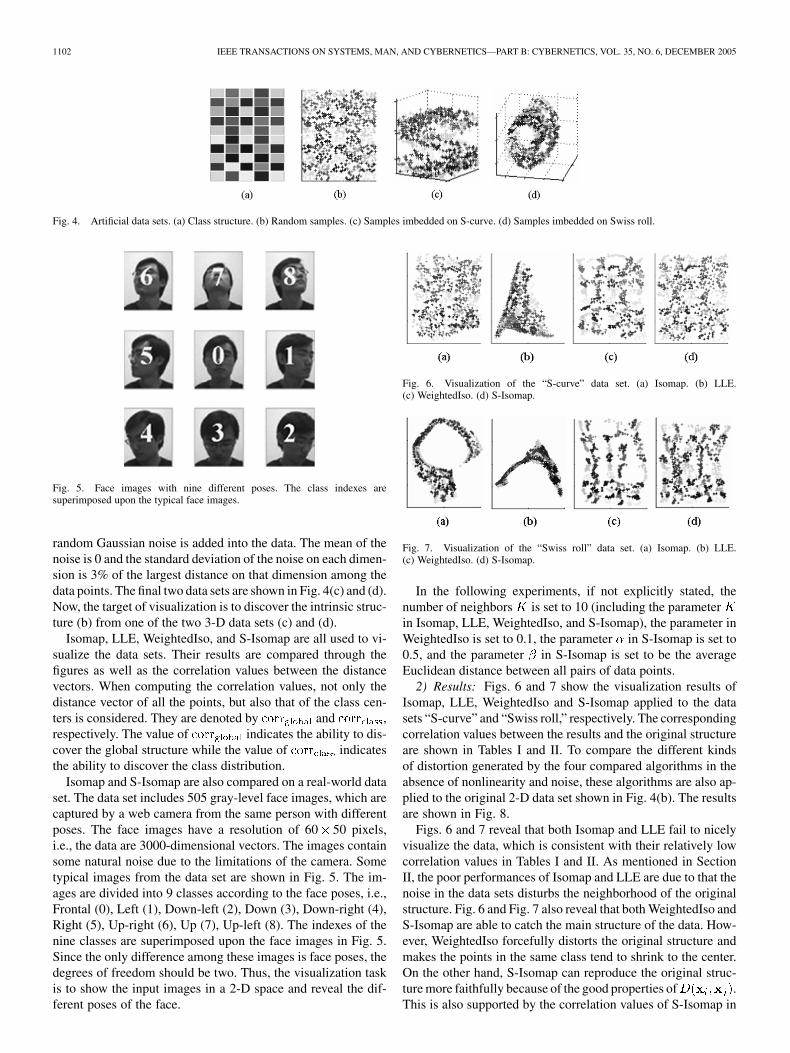
Fig. 5. Face images with nine different poses. The class indexes aresuperimposed upon the typical face images.

random Gaussian noise is added into the data. The mean of thenoise is 0 and the standard deviation of the noise on each dimen-sion is 3% of the largest distance on that dimension among thedata points. The final two data sets are shown in Fig. 4(c) and (d).Now, the target of visualization is to discover the intrinsic struc-ture (b) from one of the two 3-D data sets (c) and (d).

Isomap, LLE, WeightedIso, and S-Isomap are all used to vi-sualize the data sets. Their results are compared through thefigures as well as the correlation values between the distancevectors. When computing the correlation values, not only thedistance vector of all the points, but also that of the class cen-ters is considered. They are denoted by and ,respectively. The value of indicates the ability to dis-cover the global structure while the value of indicatesthe ability to discover the class distribution.

Isomap and S-Isomap are also compared on a real-world dataset. The data set includes 505 gray-level face images, which arecaptured by a web camera from the same person with differentposes. The face images have a resolution of 60 50 pixels,i.e., the data are 3000-dimensional vectors. The images containsome natural noise due to the limitations of the camera. Sometypical images from the data set are shown in Fig. 5. The im-ages are divided into 9 classes according to the face poses, i.e.,Frontal (0), Left (1), Down-left (2), Down (3), Down-right (4),Right (5), Up-right (6), Up (7), Up-left (8). The indexes of thenine classes are superimposed upon the face images in Fig. 5.Since the only difference among these images is face poses, thedegrees of freedom should be two. Thus, the visualization taskis to show the input images in a 2-D space and reveal the dif-ferent poses of the face.

Fig. 6. Visualization of the “S-curve” data set. (a) Isomap. (b) LLE.(c) WeightedIso. (d) S-Isomap.

Fig. 7. Visualization of the “Swiss roll” data set. (a) Isomap. (b) LLE.(c) WeightedIso. (d) S-Isomap.

In the following experiments, if not explicitly stated, thenumber of neighbors is set to 10 (including the parameterin Isomap, LLE, WeightedIso, and S-Isomap), the parameter inWeightedIso is set to 0.1, the parameter in S-Isomap is set to0.5, and the parameter in S-Isomap is set to be the averageEuclidean distance between all pairs of data points.

2) Results: Figs. 6 and 7 show the visualization results ofIsomap, LLE, WeightedIso and S-Isomap applied to the datasets “S-curve” and “Swiss roll,” respectively. The correspondingcorrelation values between the results and the original structureare shown in Tables I and II. To compare the different kindsof distortion generated by the four compared algorithms in theabsence of nonlinearity and noise, these algorithms are also ap-plied to the original 2-D data set shown in Fig. 4(b). The resultsare shown in Fig. 8.

Figs. 6 and 7 reveal that both Isomap and LLE fail to nicelyvisualize the data, which is consistent with their relatively lowcorrelation values in Tables I and II. As mentioned in SectionII, the poor performances of Isomap and LLE are due to that thenoise in the data sets disturbs the neighborhood of the originalstructure. Fig. 6 and Fig. 7 also reveal that both WeightedIso andS-Isomap are able to catch the main structure of the data. How-ever, WeightedIso forcefully distorts the original structure andmakes the points in the same class tend to shrink to the center.On the other hand, S-Isomap can reproduce the original struc-ture more faithfully because of the good properties of .This is also supported by the correlation values of S-Isomap in


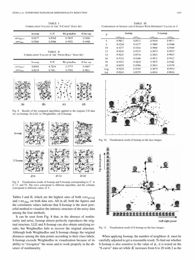
TABLE ICORRELATION VALUES OF THE “S-CURVE” DATA SET

TABLE IICORRELATION VALUES OF THE “SWISS ROLL” DATA SET

Fig. 8. Results of the compared algorithms applied to the original 2-D dataset. (a) Isomap. (b) LLE. (c) WeightedIso. (d) S-Isomap.

Fig. 9. Visualization results of Isomap and S-Isomap corresponding to K =

6; 12, and 20. The rows correspond to different algorithm, and the columnscorrespond to different values of K .

Tables I and II, which are the highest ones of bothand on both data sets. All in all, both the figures andthe correlation values indicate that S-Isomap is the most pow-erful method to visualize the intrinsic structure of the noisy dataamong the four methods.

It can be seen from Fig. 8 that, in the absence of nonlin-earity and noise, Isomap almost perfectly reproduces the orig-inal structure, LLE and S-Isomap can also obtain satisfying re-sults, but WeightedIso fails to recover the original structure.Although both WeightedIso and S-Isomap change the originaldistances among the data points according to their class labels,S-Isomap exceeds WeightedIso in visualization because of itsability to “recognize” the noise and to work properly in the ab-sence of nonlinearity.

TABLE IIICOMPARISON OF ISOMAP AND S-ISOMAP WITH DIFFERENT VALUES OF K

Fig. 10. Visualization result of Isomap on the face images.

Fig. 11. Visualization result of S-Isomap on the face images.

When applying Isomap, the number of neighbors must becarefully adjusted to get a reasonable result. To find out whetherS-Isomap is also sensitive to the value of , it is tested on the“S-curve” data set while increases from 6 to 20 with 2 as the


TABLE IVDATA SETS USED IN CLASSIFICATION

interval. Then the results are compared with those of Isomap.The correlation values are tabulated in Table III, where “Avg.”means average and “Std.” means standard deviation. The visu-alization results corresponding to 6, 12, and 20 are shownin Fig. 9.

Table III reveals that the average correlation values ofS-Isomap are significantly larger than those of Isomap whilethe standard deviations of S-Isomap are significantly smallerthan that of Isomap. Fig. 9 reveals that as increases, theresults of Isomap become significantly worse, but those ofS-Isomap do not change much. Both Table III and Fig. 8 indi-cate that S-Isomap is more accurate and less sensitive to thanIsomap. Thus, S-Isomap can be easily applied to real-worlddata without much effort on parameter tuning.

The visualization results of Isomap and S-Isomap on the faceimages are shown in Figs. 10 and 11, respectively. In the figures,the corresponding points of the successive images from up todown and from left to right are marked by black circles andlinked by lines. The nine critical face samples shown in Fig. 5are marked by gray circles and shown near the correspondingpoints.

It can be seen from Fig. 10 that Isomap can hardly reveal thedifferent face poses. Part of the up-down line is almost parallel tothe left-right line. And the arrangement of the nine face samplesis tanglesome. On the other hand, in Fig. 11, the up-down line isapproximately perpendicular to the left-right line. Thus, the hor-izontal axis represents the left-right poses, and the vertical axisrepresents the up-down poses. Moreover, the nine face samplesare mapped to the approximately right positions correspondingto the face poses. All these indicate that S-Isomap is able to ap-proximately visualize the different poses of the face images. It isworth mentioning that the face images are only roughly dividedinto nine classes, so the points in Fig. 11 tend to congregate innine groups corresponding to the nine classes. If the face im-ages can be more detailedly divided (of course there should bemore than one image in one class; otherwise, there will not be

any “intraclass” distances), the visualization result will be moreaccurate.

B. Classification

1) Methodology: In this section, S-Isomap is compared withIsomap and WeightedIso in classification. Some other well-es-tablished classification methods, including -NN classifier [4],[6], BP neural network [10], J4.8 decision tree [18], and SVM[14], [15], are also compared.

The method of using S-Isomap in classification has beendescribed in Section III-B. For convenience of discussion,“S-Isomap” is still used to indicate the three-step classificationmethod that uses S-Isomap as the first step in this experiment.The meanings of “S-Isomap” can be easily distinguished fromthe context. Isomap and WeightedIso are used in classificationin the similar way except that in the first step, S-Isomap isreplaced by Isomap and WeightedIso, respectively, and the cor-responding classification methods are still denoted by “Isomap”and “WeightedIso.” In the dimensionality reduction procedure,the dimensionality of the data is reduced to half of the original.

The parameters for most of the methods are determined em-pirically through ten-fold cross validation. That is, for each pa-rameter, several values are tested through ten-fold cross valida-tion and the best one is selected. For S-Isomap, different valuesof between 0.25 and 0.6 are tested. For WeightedIso, differentvalues of between 0.05 and 0.5 are tested. When applying

-NN algorithm, several values of from 10 to 40 are tested.The BP neural networks and the J4.8 decision trees are con-structed using WEKA [18] with the default settings. For SVM,both linear kernel and nonlinear kernel (radial basis functionwith bias 1.0) are tested and the best result is reported.

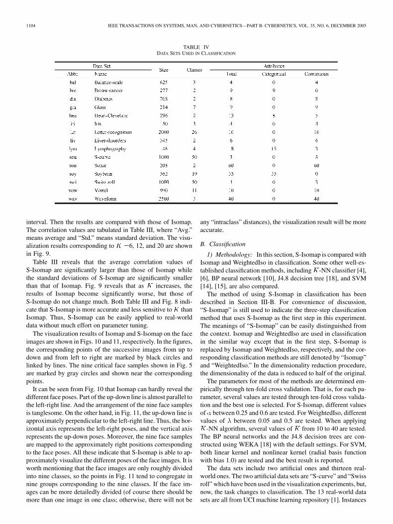
The data sets include two artificial ones and thirteen real-world ones. The two artificial data sets are “S-curve” and “Swissroll” which have been used in the visualization experiments, but,now, the task changes to classification. The 13 real-world datasets are all from UCI machine learning repository [1]. Instances


TABLE VMEAN PRECISIONS OF THE COMPARED CLASSIFICATION METHODS

that have missing values are removed. Information of all the datasets is summarized in Table IV.

It can be seen from Table IV that some data sets have cate-gorical attributes. The previous discussion on S-Isomap is onlyabout continuous data. As for categorical attributes, the distanceis computed through VDM proposed by Stanfill and Waltz [12].

On each data set, ten times ten-fold cross validation is run.That is, in each time, the original data set is randomly dividedinto ten equal-sized subsets while keeping the proportion of theinstances in different classes. Then, in each fold, one subset isused as testing set and the union of the remaining ones is used astraining set. After ten folds, each subset has been used as testingset once. The average result of these ten folds is recorded. Thisprocedure is repeated ten times and gets ten results for eachcompared algorithm. After that, the pair wise one-tailed -testis performed on the results of S-Isomap paired with every otheralgorithm at the significance level 0.025. It is worth mentioningthat the ten times ten-fold cross validation is completely separatewith those used in parameter tuning, i.e., once the parameters fora certain method on a certain data set are determined, the dataset is redivided ten times and tested.

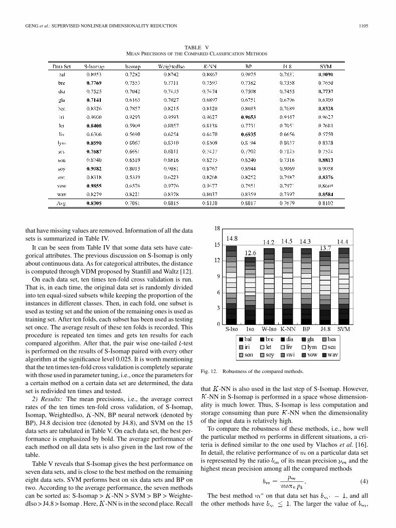
2) Results: The mean precisions, i.e., the average correctrates of the ten times ten-fold cross validation, of S-Isomap,Isomap, WeightedIso, -NN, BP neural network (denoted byBP), J4.8 decision tree (denoted by J4.8), and SVM on the 15data sets are tabulated in Table V. On each data set, the best per-formance is emphasized by bold. The average performance ofeach method on all data sets is also given in the last row of thetable.

Table V reveals that S-Isomap gives the best performance onseven data sets, and is close to the best method on the remainingeight data sets. SVM performs best on six data sets and BP ontwo. According to the average performance, the seven methodscan be sorted as: S-Isomap > -NN > SVM > BP > Weighte-dIso > J4.8 > Isomap . Here, -NN is in the second place. Recall

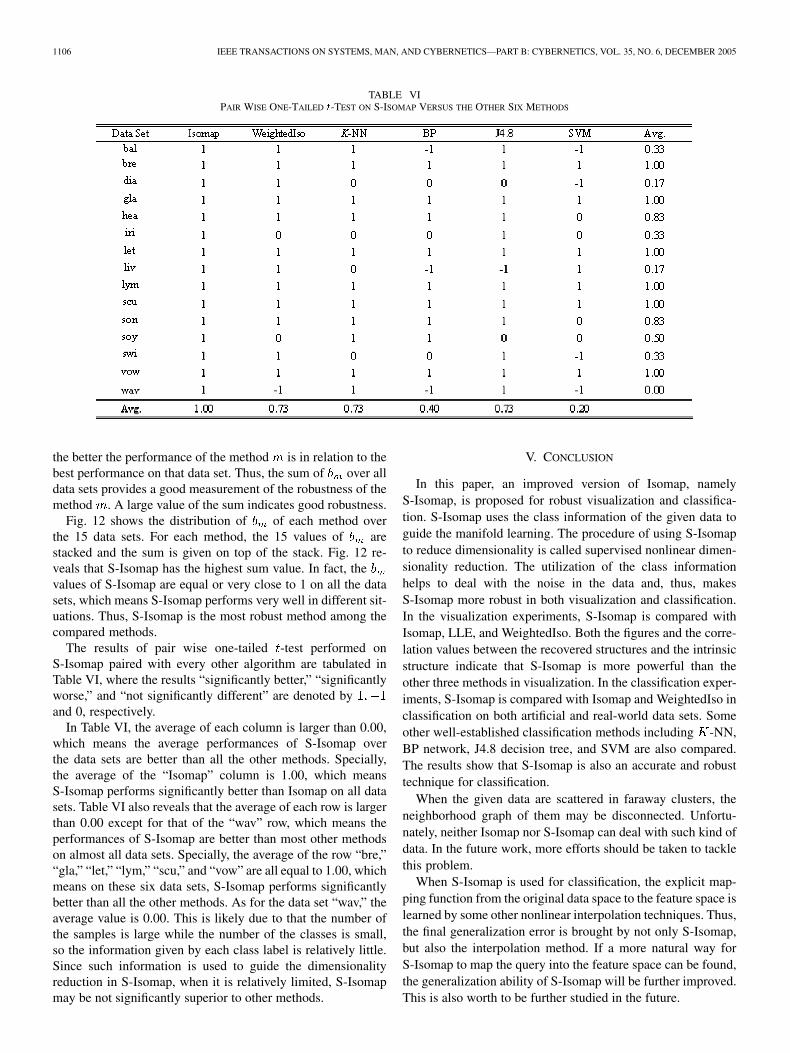
Fig. 12. Robustness of the compared methods.

that -NN is also used in the last step of S-Isomap. However,-NN in S-Isomap is performed in a space whose dimension-

ality is much lower. Thus, S-Isomap is less computation andstorage consuming than pure -NN when the dimensionalityof the input data is relatively high.

To compare the robustness of these methods, i.e., how wellthe particular method performs in different situations, a cri-teria is defined similar to the one used by Vlachos et al. [16].In detail, the relative performance of on a particular data setis represented by the ratio of its mean precision and thehighest mean precision among all the compared methods

(4)

The best method on that data set has , and allthe other methods have . The larger the value of ,


TABLE VIPAIR WISE ONE-TAILED t-TEST ON S-ISOMAP VERSUS THE OTHER SIX METHODS

the better the performance of the method is in relation to thebest performance on that data set. Thus, the sum of over alldata sets provides a good measurement of the robustness of themethod . A large value of the sum indicates good robustness.

Fig. 12 shows the distribution of of each method overthe 15 data sets. For each method, the 15 values of arestacked and the sum is given on top of the stack. Fig. 12 re-veals that S-Isomap has the highest sum value. In fact, thevalues of S-Isomap are equal or very close to 1 on all the datasets, which means S-Isomap performs very well in different sit-uations. Thus, S-Isomap is the most robust method among thecompared methods.

The results of pair wise one-tailed -test performed onS-Isomap paired with every other algorithm are tabulated inTable VI, where the results “significantly better,” “significantlyworse,” and “not significantly different” are denoted byand 0, respectively.

In Table VI, the average of each column is larger than 0.00,which means the average performances of S-Isomap overthe data sets are better than all the other methods. Specially,the average of the “Isomap” column is 1.00, which meansS-Isomap performs significantly better than Isomap on all datasets. Table VI also reveals that the average of each row is largerthan 0.00 except for that of the “wav” row, which means theperformances of S-Isomap are better than most other methodson almost all data sets. Specially, the average of the row “bre,”“gla,” “let,” “lym,” “scu,” and “vow” are all equal to 1.00, whichmeans on these six data sets, S-Isomap performs significantlybetter than all the other methods. As for the data set “wav,” theaverage value is 0.00. This is likely due to that the number ofthe samples is large while the number of the classes is small,so the information given by each class label is relatively little.Since such information is used to guide the dimensionalityreduction in S-Isomap, when it is relatively limited, S-Isomapmay be not significantly superior to other methods.

V. CONCLUSION

In this paper, an improved version of Isomap, namelyS-Isomap, is proposed for robust visualization and classifica-tion. S-Isomap uses the class information of the given data toguide the manifold learning. The procedure of using S-Isomapto reduce dimensionality is called supervised nonlinear dimen-sionality reduction. The utilization of the class informationhelps to deal with the noise in the data and, thus, makesS-Isomap more robust in both visualization and classification.In the visualization experiments, S-Isomap is compared withIsomap, LLE, and WeightedIso. Both the figures and the corre-lation values between the recovered structures and the intrinsicstructure indicate that S-Isomap is more powerful than theother three methods in visualization. In the classification exper-iments, S-Isomap is compared with Isomap and WeightedIso inclassification on both artificial and real-world data sets. Someother well-established classification methods including -NN,BP network, J4.8 decision tree, and SVM are also compared.The results show that S-Isomap is also an accurate and robusttechnique for classification.

When the given data are scattered in faraway clusters, theneighborhood graph of them may be disconnected. Unfortu-nately, neither Isomap nor S-Isomap can deal with such kind ofdata. In the future work, more efforts should be taken to tacklethis problem.

When S-Isomap is used for classification, the explicit map-ping function from the original data space to the feature space islearned by some other nonlinear interpolation techniques. Thus,the final generalization error is brought by not only S-Isomap,but also the interpolation method. If a more natural way forS-Isomap to map the query into the feature space can be found,the generalization ability of S-Isomap will be further improved.This is also worth to be further studied in the future.


ACKNOWLEDGMENT

The authors would like to thank the anonymous reviewers fortheir comments and suggestions which greatly improved thispaper.

REFERENCES

[1] C. Blake, E. Keogh, and C. J. Merz. (1998) “UCI repository of machinelearning databases,” Dept. Inf. Comp. Sci., Univ. California, Irvine. [On-line]. Available: http://www.ics.uci.edu/~mlearn/MLRepository.html

[2] P. Comon, “Independent component analysis: A new concept?,” SignalProcess., vol. 36, no. 3, pp. 287–314, 1994.

[3] T. Cox and M. Cox, Multidimensional Scaling. London, U.K.:Chapman & Hall, 1994.

[4] T. K. Ho, “Nearest neighbors in random subspaces,” in Lecture Notesin Computer Science: Advances in Pattern Recognition. Berlin, Ger-many: Springer, 1998, pp. 640–948.

[5] I. T. Jolliffe, Principal Component Analysis. New York: Springer,1986.

[6] D. Lowe, “Similarity metric learning for a variable-kernel classifier,”Neural Comput., vol. 7, no. 1, pp. 72–85, 1995.

[7] K. V. Mardia, J. T. Kent, and J. M. Bibby, Multivariate Anal-ysis. London, U.K.: Academic, 1979.

[8] J. Quinlan, C4.5: Programs for Machine Learning. San Francisco, CA:Morgan-Kaufmann, 1993.

[9] S. T. Roweis and L. K. Saul, “Nonlinear dimensionality reduction bylocal linear embedding,” Science, vol. 290, no. 5500, pp. 2323–2326,2000.

[10] D. E. Rumelhart, G. E. Hinton, and R. J. Williams, “Learning represen-tations by backpropagating errors,” Nature, vol. 323, no. 9, pp. 318–362,1986.

[11] L. K. Saul and S. T. Roweis, “Think globally, fit locally: Unsupervisedlearning of low dimensional manifolds,” J. Mach. Learn. Res., vol. 4, pp.119–155, 2003.

[12] C. Stanfill and D. Waltz, “Toward memory-based reasoning,” Commun.ACM, vol. 29, no. 12, pp. 1213–1228, 1986.

[13] J. B. Tenenbaum, V. de Silva, and J. C. Langford, “A global geometricframework for nonlinear dimensionality reduction,” Science, vol. 290,no. 5500, pp. 2319–2323, 2000.

[14] V. Vapnik, The Nature of Statistical Learning Theory. New York:Springer, 1995.

[15] , Statistical Learning Theory. New York: Wiley, 1998.[16] M. Vlachos, C. Domeniconi, D. Gunopulos, G. Kollios, and N. Koudas,

“Non-linear dimensionality reduction techniques for classification andvisualization,” in Proc. 8th ACM SIGKDD Int. Conf. Knowledge Dis-covery and Data Mining, Edmonton, AB, Canada, 2002, pp. 645–651.

[17] P. D. Wasserman, Advanced Methods in Neural Computing. NewYork: Van Nostrand Reinhold, 1993.

[18] I. H. Witten and E. Frank, Data Mining: Practical Machine LearningTools With Java Implementations. San Francisco, CA: Morgan Kauf-mann, 1999.

Xin Geng received the B.Sc. and M.Sc. degrees incomputer science from Nanjing University, Nanjing,China, in 2001 and 2004, respectively.

Currently, he is a Research and Teaching Assistantwith the Department of Computer Science and Tech-nology, Nanjing University, and a member of theLAMDA group. He has been a reviewer for severalinternational conferences. His research interestsinclude machine learning, pattern recognition, andcomputer vision.

De-Chuan Zhan received the B.Sc. degree incomputer science from Nanjing University, Nanjing,China, in 2004. He is currently pursuing the M.Sc.degree at the Department of Computer Science andTechnology, Nanjing University, supervised by Prof.Z.–H. Zhou.

He is a member of the LAMDA group at NanjingUniversity. His research interests include machinelearning and pattern recognition.

Mr. Zhan received the Peoples’ Scholarship foroutstanding undergraduate work

Zhi-Hua Zhou (S’00–M’01) received the B.Sc.,M.Sc., and Ph.D. degrees in computer science fromNanjing University, Nanjing, China, in 1996, 1998,and 2000, respectively, all with highest honors.

He joined the Department of Computer Scienceand Technology, Nanjing University, as a Lecturerin 2001, and he is currently a Professor and Headof the LAMDA group. His research interests in-clude artificial intelligence, machine learning, datamining, pattern recognition, information retrieval,neural computing, and evolutionary computing. He

has published over 40 technical papers in refereed international journals orconference proceedings in these areas.

Dr. Zhou won the Microsoft Fellowship Award (1999), the National ExcellentDoctoral Dissertation Award of China (2003), and the Award of National Out-standing Youth Foundation of China (2004). He is an associate editor of Knowl-edge and Information Systems, and he is on the editorial boards of the ArtificialIntelligence in Medicine, the International Journal of Data Warehousing andMining, the Journal of Computer Science and Technology, and the Journal ofSoftware. He served as the organizing Chair of the 7th Chinese Workshop onMachine Learning (2000), program Co-Chair of the 9th Chinese Conference onMachine Learning (2004), and program committee member for numerous in-ternational conferences. He is a Senior Member of China Computer Federation(CCF), the Vice Chair of the CCF Artificial Intelligence and Pattern Recog-nition Society, a Councilor of the Chinese Association of Artificial Intelligence(CAAI), and the Vice Chair and Chief Secretary of the CAAI Machine LearningSociety.

Documents

1098 IEEE TRANSACTIONS ON SYSTEMS, MAN, AND CYBERNETICS ...syllabus.cs.manchester.ac.uk/pgt/2019/COMP61021/... · 1098 IEEE TRANSACTIONS ON SYSTEMS, MAN, AND CYBERNETICS—PART B: