IEEE TRANSACTIONS ON CYBERNETICS 1 Manifold Partition

IEEE TRANSACTIONS ON CYBERNETICS 1

Manifold Partition Discriminant AnalysisYang Zhou and Shiliang Sun

Abstract—We propose a novel algorithm for supervised dimensionality reduction named Manifold Partition Discriminant Analysis(MPDA). It aims to find a linear embedding space where the within-class similarity is achieved along the direction that is consistent withthe local variation of the data manifold, while nearby data belonging to different classes are well separated. By partitioning the datamanifold into a number of linear subspaces and utilizing the first-order Taylor expansion, MPDA explicitly parameterizes the connectionsof tangent spaces and represents the data manifold in a piecewise manner. While graph Laplacian methods capture only the pairwiseinteraction between data points, our method capture both pairwise and higher order interactions (using regional consistency) betweendata points. This manifold representation can help to improve the measure of within-class similarity, which further leads to improvedperformance of dimensionality reduction. Experimental results on multiple real-world data sets demonstrate the effectiveness of theproposed method.

Index Terms—Discriminant Analysis, Supervised Learning, Manifold Learning, Tangent Space

✦

1 INTRODUCTION

Linear Discriminant Analysis (LDA) is a classical su-pervised dimensionality reduction method. It aims tofind an optimal low-dimensional projection along whichdata points from different classes are far away fromeach other, while those belonging to the same class areas close as possible. In the resultant low-dimensionalspace, the performance of classifiers could be improved.Because of this, LDA is especially useful for classificationtasks. Due to its effectiveness, LDA is widely employedin different applications such as face recognition andinformation retrieval [1], [2], [3], [4]. However, when theinput data are multimodal or mainly characterized bytheir variances, LDA cannot perform very well. This iscaused by the assumption implicitly adopted by LDAthat data points belonging to each class are generatedfrom multivariate Gaussian distributions with the samecovariance matrix but different means. If data are formedby several separate clusters or lie on a manifold, thisassumption is violated, and thus LDA obtains undesiredresults.

To solve this problem, some extensions of LDA havebeen proposed, which resort to discovering local datastructures. Marginal Fisher Analysis (MFA) [5] aimsto gather the nearby examples of the same class, andseparate the marginal examples belonging to differentclasses. Locality Sensitive Discriminant Analysis (LSDA)[6] maps data points into a subspace where the exampleswith the same label at each local area are close, while thenearby examples from different classes are apart from

• Yang Zhou and Shiliang Sun (corresponding author) are withShanghai Key Laboratory of Multidimensional Information Processing,Department of Computer Science and Technology, East China NormalUniversity, 500 Dongchuan Road, Shanghai 200241, P. R. China (email:[email protected], [email protected])

Manuscript received Dec. 21, 2014; revised Apr. 2, 2015, Sep. 10, 2015 andJan. 21, 2016; accepted Feb. 9, 2016.

each other. Local Fisher Discriminant Analysis (LFDA)[7] also focuses on discovering local data structures. Itcan be viewed as performing LDA on the local areaaround each data point. LFDA is a very effective al-gorithm and has many applications. Recently, LFDA(combined with PCA) was applied to the pedestrian re-identification problem and achieved the state-of-the-artperformance [8]. Despite of different names and motiva-tions, these methods, in fact, fall into the same graphLaplacian based framework. All of them employ theLaplacian matrix on specific graphs to characterize datastructures locally, and share the same idea that if nearbyexamples xi, xj have the same class label y, they shouldbe projected as close as possible, otherwise, they shouldbe well separated. By exploiting the local structuresaround each data point, they are able to process the dataon which LDA cannot achieve reasonable results. Aswidely recognized, graphs are often used as a proxy forthe manifold. Therefore, these methods, to some extent,can be viewed as the combinations of manifold learningand LDA.

Although the above methods overcome the drawbackof LDA, they rely on the graph Laplacian to capturethe manifold structure, where only pairwise differencesare considered whereas regional consistency is ignored.The regional consistency can be characterized by tangentspaces of the data manifold, which could be very usefulto enhance the performance of discriminant analysisin some situations [9] [10]. Moreover, the definition ofcloseness of these graph Laplacian based methods israther vague. Along which direction can we decide ifthe closeness of the mapped data points is achieved? Weadvocate that in order to preserve the manifold structureas much as possible, the closeness of the embeddingsshould be achieved along the direction that is consistentwith the local variation of the data manifold.

During recent years, tangent space based methodshave received considerable interest in the area of man-


ifold learning [10], [11], [12], [13]. They utilize tangentspaces to estimate and extract the topological and ge-ometrical structure of the underlying manifold. LocalTangent Space Alignment (LTSA) [11] constructs tangentspaces at each data point and then aligns them to obtaina global coordinate through minimizing the reconstruc-tion error. Similar to LTSA, Manifold Charting [12] triesto unfold the manifold by aligning local charts. TangentSpace Intrinsic Manifold Regularization (TSIMR) [10]estimates a local linear function on the manifold whichhas constant manifold derivatives. Parallel Vector FieldEmbedding (PFE) [13] represents a function along themanifold from the perspective of vector fields and re-quires the vector field at each data point to be as parallelas possible. Due to exploiting the regional consistencyreflected by tangent spaces, these tangent space basedmethods work well for representing the manifold struc-ture. However, because of their unsupervised nature,they have no ability to capture the discriminative infor-mation from class labels, and thus are not optimal forsupervised dimensionality reduction. Then how shouldwe utilize the regional consistency of tangent spaces toimprove the performance of supervised dimensionalityreduction?

Besides the methods mentioned above, there are manyother works that have been done in the field of dimen-sionality reduction. Supervised Local Subspace Learn-ing (SL2) [14] learns a mixture of local tangent spacesthat are robust to under-sampled regions for continuoushead pose estimation, so that it can avoid overfittingand be robust to noise. Linear Spherical DiscriminantAnalysis (LSDA) [15] performs discriminant analysisbased on the cosine distance metric to improve speakerclustering performance. By building a sparse projectionmatrix for dimension reduction, Double Shrinking Al-gorithm (DSA) [16] compresses image data on both di-mensionality and cardinality to obtain better embeddingor classification performance. Least-Squares DimensionReduction (LSDR) [17] adopts a squared-loss variant ofmutual information as a dependency measure to performsufficient dimensionality reduction. Wang et al. proposedan exponential framework for dimensionality reduction[18]. By using matrix exponential to measure data sim-ilarity, this framework emphasizes small distance pairs,and can avoid the small sample size problem. Althoughall of these methods have their own merits, none of themsolves the above mentioned two problems.

In this paper, we propose a novel supervised di-mensionality reduction method called Manifold PartitionDiscriminant Analysis (MPDA), which solves the abovetwo problems. In MPDA, pairwise differences and piece-wise regional consistency are considered simultaneously,so that the manifold structure can be well preserved.MPDA aims to find a linear embedding space wherethe within-class similarity is achieved along the directionthat is consistent with the local variation of the data man-ifold, while nearby data belonging to different classesare well separated. Compared with existing methods,

MPDA has several desirable properties that should behighlighted:

• MPDA partitions the data manifold into a numberof non-overlapping linear subspaces and discoversregional manifold structures in a piecewise manner.

• With the partitioned manifold, MPDA is able toconstruct tangent spaces with varied numbers of di-mensions. This provides MPDA with more flexibil-ity to handle non-uniformly distributed or complexdata.

• By using the first-order Taylor expansion, MPDAestablishes a manifold representation which is char-acterized by both the pairwise differences and piece-wise regional consistency of the underlying mani-fold.

• Thanks to the proposed manifold representation,MPDA improves the measure of within-class sim-ilarity, and is able to obtain a projection that isconsistent with the local variation of the underlyingmanifold.

The rest of this paper is organized as follows. InSection 2, we briefly introduce the graph Laplacian basedframework, under which many supervised dimensional-ity reduction methods can be considered within the samecategory. Then the Manifold Partition Discriminant Anal-ysis (MPDA) algorithm is presented in Section 3. Sec-tion 4 discusses the connection and difference betweenMPDA and related works. In Section 5, MPDA is testedon multiple real-world data sets compared with existingsupervised dimensionality reduction algorithms. Finally,we give concluding remarks in Section 6.

2 GRAPH LAPLACIAN BASED FRAMEWORKFOR DISCRIMINANT ANALYSIS

Representing data on a specific graph is a popular way tocharacterize the relationships among data points. Givenan undirected weighted G = {X, W} with a vertex setX and a symmetric weight matrix W ∈ R

n×n, theserelationships can be easily characterized by G, whereeach example serves as a vertex of G, and W records theweight on the edge of each pair of vertices. Generally, iftwo examples xi and xj are “close”, the correspondingweight Wij is large, whereas if they are “far away”,then the Wij is small. Provided a certain W , the intrinsicgeometry of graph G can be represented by the Laplacianmatrix [19], which is defined as

L = D −W, (1)

where D is a diagonal matrix with the i-th diagonalelement being Dii =

∑

j 6=i Wij . The Laplacian matrixis capable of representing certain geometry of data ac-cording to a specific weight matrix. This property isvery helpful for developing dimensionality reductionmethods.

Let X be a data set consisting of n examples and labels,{(xi, yi)}ni=1

, where xi ∈ Rd denotes a d-dimensional


example, yi ∈ {1, 2, . . . , C} denotes the class label cor-responding to xi, and C is the total number of classes.Classical LDA aims to find an optimal linear projection t

along which the between-class scatter is maximized andthe within-class scatter is minimized [20]. The objectivefunction of LDA can be written as:

t∗ = arg maxt

t⊤Sbt

t⊤Swt, (2)

where ⊤ denotes the transpose of a matrix or a vector, Sb

and Sw denote the between-class and within-class scattermatrices, respectively. The definitions of Sb and Sw aregiven as follows:

Sb =C∑

c=1

nc(µc − µ)(µc − µ)⊤, (3)

Sw =

C∑

c=1

∑

{i|yi=c}

(xi − µc)(xi − µc)⊤, (4)

where nc is the number of data from the c-th class,µ = 1

n

∑n

i=1xi is the mean of all the data points, and

µc = 1

nc

∑

{i|yi=c} xi is the mean of the data from classc. Apart from the above formulations, Sb and Sw can alsobe formulated via the graph Laplacian [7]:

Sb =∑

ij

W bij‖xi − xj‖

2 = 2XLbX⊤, (5)

Sw =∑

ij

Wwij ‖xi − xj‖

2 = 2XLwX⊤, (6)

where Lw and Lb are the Laplacian matrices constructedby the weight matrices Ww and W b with

W bij =

{

(1/n− 1/nc) if yi = yj = c

1/n if yi 6= yj ,

Wwij =

{

1/nc if yi = yj = c

0 if yi 6= yj .

The objective function (2) can be converted to a gener-alized eigenvalue problem:

XLwX⊤t = λXLbX⊤t (7)

whose solution can be easily given by the eigenvectorwith respect to the largest eigenvalue. From the aboveformulations, it is clear that the graph Laplacian playsa key role in deriving LDA, where the weight matricesW b and Ww measure the similarity of each pair of datapoints, and their characteristics varies as the criterion ofsimilarity changes. This provides a general and flexibleframework to develop new dimensionality reductionalgorithms by constructing appropriate Laplacian matri-ces.

In order to improve the performance of LDA, manylocal structure based extensions of LDA have been pro-posed in the recent decades. Representative methodsinclude Marginal Fisher Analysis (MFA) [5], LocalitySensitive Discriminant Analysis (LSDA) [6], Local Fisher

Discriminant Analysis (LFDA) [7], etc. Unlike traditionalLDA, they compute the between-class and within-classscatter based on local data structures rather than theglobal mean values. Although these methods improvethe performance of discriminant analysis by solving theproblem caused by the improper assumption adopted byLDA, none of them extends beyond the graph Laplacianbased framework. Their differences merely lie in thedifferent ways of constructing the Laplacian matrices Lb

and Lw.In spite of its effectiveness, the graph Laplacian based

framework still has several limitations. The between-class and within-class scatter are computed by onlyaggregating all pairwise differences between data pointsacross the entire graph, whereas the regional consistency,which is reflected by the regional structure around a localarea of the underlying manifold, is ignored. Moreover,by minimizing the aggregation of within-class data pairs(6), the objective function (2) tends to find a directionalong which some “averaged” within-class similarity isachieved. However, it is unclear that how the “averaged”similarity can precisely reflect the topological and geo-metrical structure of the underlying manifold.

3 MANIFOLD PARTITION DISCRIMINANTANALYSIS

In this section, we propose a novel supervised dimen-sionality reduction algorithm named Manifold PartitionDiscriminant Analysis (MPDA). Unlike previous meth-ods that mainly rely on the graph Laplacian [5], [6], [7],MPDA exploits both pairwise differences and piecewiseregional consistency to preserve the manifold structure.It aims to find a linear embedding space where thewithin-class similarity is achieved along the directionthat is consistent with the local variation of the data man-ifold, while nearby data belonging to different classesare well separated. To this end, we first need to extractthe piecewise consistency from the data manifold, whichcan be achieved by partitioning the data manifold intonon-overlapping pieces, and estimating tangent spacesfor each piece. Then we can represent the data manifoldby combining pairwise differences with piecewise con-sistency. The resultant manifold representation is able tocharacterize the local variation of the data manifold, andimprove the measure of within-class similarity, whicheventually leads to the MPDA algorithm. Specifically, wemainly solve the following problems:

P1 How to partition the data manifold into a numberof non-overlapping pieces, and estimate an accuratetangent space?

P2 How to combine pairwise differences with piece-wise regional consistency in representing the datamanifold?

P3 How to find a linear subspace where the within-class similarity is achieved along the direction thatis consistent with the local variation of the datamanifold?


Next, we first solve P2 and P3 in Section 3.1 and 3.2,respectively, and defer the treatment of P1 to Section 3.3.

3.1 Manifold Representation

In order to combine pairwise differences with piecewiseregional consistency in representing the data manifold,we are interested in estimating a function f definedon an m-dimensional smooth manifold M, where M isembedded in R

d. This function f can serve as a directconnection between the data representation in d and m-dimensional spaces. For simplicity, we first consider torepresent data in a one-dimensional Euclidean space R.Define f : R

d → R as a function along the manifoldM. Let Tx0

M be the tangent space of x0 on M, wherex0 ∈ R

d is a single point on the manifold M. Accord-ing to the first-order Taylor expansion at x0, f can beexpressed as follows [10], [13], [21]:

f(x) = f(x0) + v⊤x0

ux0(x) + O(‖x− x0‖

2),

where ux0(x) = T⊤

x0(x−x0) is an m-dimensional vector

which gives a representation of x in the tangent spaceTx0M. Tx0

∈ Rd×m is a matrix formed by the or-

thonormal bases of Tx0M, and characterizes the regional

consistency of the manifold structure around x0. Gener-ally, Tx0

can be estimated by performing PCA on theneighborhood of x0 [11], [22]. vx0

is an m-dimensionaltangent vector and represents the manifold derivative off at x0 with respect to ux0

(x), which reflects the localvariation of the manifold at x0.

Given two nearby data points z and z′ lying on themanifoldM, we can use the first-order Taylor expansionat z′ to express f(z) as follows:

f(z) = f(z′) + v⊤z′T⊤

z′(z − z′) + O(‖z − z′‖2). (8)

If M is smooth enough, the second-order derivatives off tend to vanish. Furthermore, when z and z′ are closeto each other, ‖z − z′‖2 becomes very small. Therefore,the remainder in (8) can be omitted, which leads to:

f(z) ≈ f(z′) + v⊤z′T⊤

z′(z − z′). (9)

With the above results, it is clear that for any nearbydata points z and z′ lying on the manifold M, the low-dimensional embeddings f(z) and f(z′) should satisfy(9), and the difference between both sides of (9) shouldbe as small as possible. This can serve as a good criterionto preserve the manifold structure, which establishes theconnection between each pair of nearby data points.

Assume that the data manifold can be well approx-imated by the union of a number of non-overlappinglinear subspaces. In this case, each linear subspace canserve as a tangent space, and each tangent space hasa tangent vector. With the partitioned manifold, we areable to construct tangent spaces and tangent vectors foreach linear subspace rather than each data point. If z′

lies in a tangent space TpM with a tangent vector vp, (9)becomes:

f(z) ≈ f(z′) + v⊤p T⊤

p (z − z′), (10)

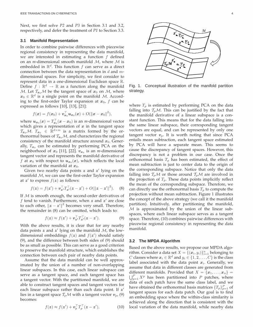
Fig. 1. Conceptual illustration of the manifold partitionstrategy.

where Tp is estimated by performing PCA on the datafalling into TpM. This can be justified by the fact thatthe manifold derivative of a linear subspace is a con-stant function. This means that for the data falling intothe same linear subspace, their corresponding tangentvectors are equal, and can be represented by only onetangent vector vp. It is worth noting that since PCAentails mean subtraction, each tangent space estimatedby PCA will have a separate mean. This seems tocause the discrepancy of tangent spaces. However, thisdiscrepancy is not a problem in our case. Once theorthonormal basis Tp has been estimated, the effect ofmean subtraction is just to center data to the origin ofthe corresponding subspace. Notice that only the datafalling into TpM or those around TpM are involved inthe projection of Tp. These data points implicitly reflectthe mean of the corresponding subspace. Therefore, wecan directly use the orthonormal basis Tp to compute theprojection without mean subtraction. Figure 1 illustratesthe concept of the above strategy (we call it the manifoldpartition). Intuitively, after partitioning the manifold,M is approximated by the union of the linear sub-spaces, where each linear subspace serves as a tangentspace. Therefore, (10) combines pairwise differences withpiecewise regional consistency in representing the datamanifold.

3.2 The MPDA Algorithm

Based on the above results, we propose our MPDA algo-rithm. Consider a data set X = {(xi, yi)}ni=1

belonging toC classes where xi ∈ R

d and yi ∈ {1, 2, . . . , C} is the classlabel associated with the data point xi. Generally, weassume that data in different classes are generated fromdifferent manifolds. Provided that X = {x1, . . . , xn} =⋃P

p=1Xp has been partitioned into P patches, where

data of each patch have the same class label, and wehave obtained the orthonormal basis matrices {Tp}Pp=1

oftangent spaces for each data patch. Our goal is to findan embedding space where the within-class similarity isachieved along the direction that is consistent with thelocal variation of the data manifold, while nearby data


belonging to different classes are well separated.

In order to gather within-class data based on themanifold structure, we first construct the within-classgraph G = {X, W} to represent the geometry of the datamanifold. If xi is among the k-nearest neighbors of xj

with yi = yj , an edge connecting xi to xj is added withthe weight Wij = Wji = 1. If there is no edge connectingxi to xj , Wij = 0. With the results in Section 3.1, for eachpair of nearby within-class data points, we can obtain:

f(xi) ≈ f(xj) + v⊤πj

T⊤πj

(xi − xj), (11)

f(xj) ≈ f(xi) + v⊤πi

T⊤πi

(xj − xi). (12)

We require the difference between both sides of (11) tobe as small as possible. In the scenario of linear dimen-sionality reduction, f(x) represents a one-dimensionalembedding of x, and we aim to find a linear projection.To this end, f(x) is further approximated as a linearfunction f(x) = t⊤x where t ∈ R

d is a linear projectionvector. Then, if nearby data points xi, xj belong to thesame class, we can measure their similarity as follows:

(

f(xi)− f(xj)− v⊤πj

T⊤πj

(xi − xj))2

=(

t⊤(xi − xj)− v⊤πj

T⊤πj

(xi − xj))2

, (13)

where πi ∈ {1, . . . , P} is an index indicating the patch xi

belongs to. Moreover, we also need to measure the sim-ilarity between nearby tangent spaces. By substituting(11) into (12), we have:

(Tπjvπj− Tπi

vπi)⊤(xi − xj) ≈ 0.

From the above equation, we know that the two vec-tors are approximately perpendicular or the row vector(Tπj

vπj−Tπi

vπi)⊤ approximately equals to a zero vector.

However, the perpendicular case can not be satisfiedfor every pair of nearby data points on the manifold.For instance, consider there are three nearby data pointson the manifold. Each pair of them should satisfy theabove equation, while only two of them are, in general,justified in the perpendicular case. On the other side,the case of zero row vectors can be justified for all thedata pairs, and leads to Tπj

vπj≈ Tπi

vπi. Finally, by

multiplying both sides of this equation with T⊤πi

andusing T⊤

πiTπi

= I , it follows that:

vπi≈ T⊤

πiTπj

vπj. (14)

It is clear that for each pair of nearby tangent spaces thedifference between both sides of (14) should be as smallas possible. Therefore, the similarity between nearbytangent spaces can be measured as follows:

‖vπi− T⊤

πiTπj

vπj‖22. (15)

With the above results, the data manifold with respectto each class can be estimated by relating data with adiscrete weight Wij , which leads to an objective function

as follows:

mint,v

n∑

i,j

Wij

[

(

t⊤(xi − xj)− v⊤πj

T⊤πj

(xi − xj))2

+ γ‖vπi− T⊤

πiTπj

vπj‖22

]

,

(16)

where γ is a trade-off parameter controlling the influencebetween (13) and (15). It is clear that if xi and xj

belong to the same class and fall into the same tangentspace, their similarity only depends on their pairwisedifference. If xi and xj belong to the same class butlie in different tangent spaces, apart from the pairwisedifference, their similarity also depends on the anglebetween vπj

and T⊤πj

(xi −xj), which means that xi andxj can be viewed as similar data points when vπj

andT⊤

πj(xi − xj) have similar directions. Since vπj

reflectsthe varying direction of the data manifold around xj ,by optimizing (16), we can deem that the within-classsimilarity is achieved along the direction that is consis-tent with the local variation of the data manifold.

It is worth noting that the above derivation is basedon the first-order Taylor expansion of the function f . Ifwe employ the zero-order Taylor expansion, the termsrelated to vπi

(i = 1, . . . , n) vanish. Then the objectivefunction is simplified as follows:

mint

n∑

i,j

Wij

(

t⊤xi − t⊤xj

)2

= mint

2t⊤XLX⊤t,

where L = D − W is the Laplacian matrix and D isa diagonal matrix with the i-th diagonal element beingDii =

∑

j 6=i Wij . This formulation is identical to thegraph Laplacian based within-class scatter (6). From theaspect of manifold approximations, this means that intheory the proposed method is able to approximatethe underlying manifold with a smaller approximationerror O(||xi − xj ||2) than the graph Laplacian whoseapproximation error is O(||xi − xj ||). Compared with(16), the graph Laplacian based scatter fails to considerthe regional consistency that is explicitly parameterizedby the proposed manifold representation. Although itcan implicitly reflect regional relationships by mini-mizing the distance between each pair of nearby datapoints, the graph Laplacian has no ability to capturethe regional consistency which is determined by all thenearby data around a given data point. On the otherhand, the proposed manifold representation is capableof preserving both the pairwise geometry and the piece-wise regional consistency, and thus can capture morestructural information from the data manifold than thegraph Laplacian. In other word, (16) better measures thewithin-class similarity than the graph Laplacian basedscatter (6), because it can extract the regional consistencyof each tangent space, and explicitly establishes theconnections among tangent spaces by estimating tangentvectors {vp}Pp=1

.Notice that although we assume that the data manifold

can be approximated by a union of piece-wise subspaces,


it does not mean that the proposed manifold repre-sentation is inferior to the graph Laplacian. To verifythis, we can split the within-class objective function (16)into two parts. The first part includes the terms relatedto v, and the second part has the other terms. Thepiece-wise manifold assumption only affects the firstpart, while the second part is still based on the genericmanifold assumption. In fact, the second part of (16)is just identical to the graph Laplacian based within-class scatter. This implies that the proposed manifoldrepresentation is at least as good as, if not better than,the graph Laplacian, as each tangent vector vπi

can be azero vector.

To separate data in different classes, we construct abetween-class graph G′ = {X, W ′}. If yi 6= yj , we addan edge between xi and xj with the weight W ′

ij = 1/n.If yi = yj , the corresponding weight is set to be W ′

ij =Aij(1/n−1/nc). nc is the number of data points from thec-th class, and Aij is a weight that indicates the similaritybetween xi and xj , whose definition is given as follows:

Aij =

{

exp(− ‖xi−xj‖2

σiσj) if i ∈ Nk(j) or j ∈ Nk(i)

0 else,

where Nk(i) denotes the k-nearest neighbor set of xi,and σi is heuristically set to be the distance between xi

and its k-th nearest neighbor. Then we can formulate thefollowing objective function to separate nearby between-class data points:

maxt

n∑

i,j

W ′ij(t

⊤xi − t⊤xj)2. (17)

The methods for constructing G′ have been well studiedin the literature [5], [6]. Here, we employed the one in[7] because of its effectiveness in enhancing the between-class separability.

It is easy to see that (16) can be reformulated as acanonical matrix quadratic as ( t⊤ v⊤ )S( t⊤ v⊤ )⊤

where S is a (d + mP ) × (d + mP ) positive semi-definite matrix and v = (v⊤

1, v⊤

2, . . . , v⊤

P )⊤. Due tothe space limitation, the detailed derivation of S isprovided in the supplementary material, which is amodification of the derivation of a similar quantityused in [10]. By simple algebra formulations, (17) can

also be reduced to

(

t

v

)⊤(

2XL′X⊤0

0 0

)(

t

v

)

=

( t⊤ v⊤ )S′( t⊤ v⊤ )⊤, where L′ is the Laplacianmatrix constructed by W ′. In order to preserve the man-ifold structure while separating nearby between-classdata points, we can optimize the objective functions (16)and (17) simultaneously, which leads to the followingobjective function:

argmaxf

f⊤S′f

f⊤(S + αI)f, (18)

where we have defined f = (t⊤, v⊤)⊤, and the Tikhonovregularizer with a trade-off parameter α has been em-ployed to avoid the numerical singularity of S.

Algorithm 1 MPDA

Input:Labeled data {xi|xi ∈ R

d},Class labels {yi|yi ∈ {1, 2, . . . , C}}ni=1

;Dimensionality of embedding space m (1 ≤ m ≤ d);Trade-off parameters γ (γ > 0).

Output:d× r transformation matrix T .

Apply certain method to partition the data in eachclass into a total of P patches {Xp}Pp=1

;for p = 1 to P do

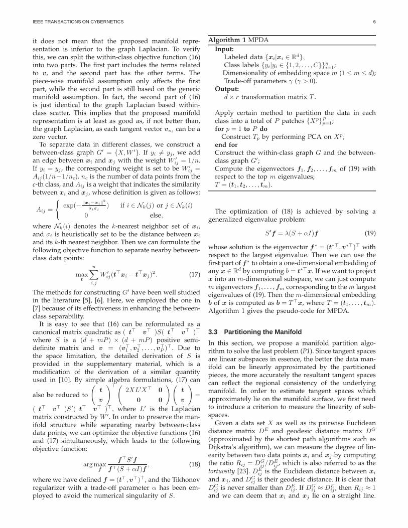
Construct Tp by performing PCA on Xp;end forConstruct the within-class graph G and the between-class graph G′;Compute the eigenvectors f1, f2, . . . , fm of (19) withrespect to the top m eigenvalues;T = (t1, t2, . . . , tm).

The optimization of (18) is achieved by solving ageneralized eigenvalue problem:

S′f = λ(S + αI)f (19)

whose solution is the eigenvector f∗ = (t∗⊤, v∗⊤)⊤ withrespect to the largest eigenvalue. Then we can use thefirst part of f∗ to obtain a one-dimensional embedding ofany x ∈ R

d by computing b = t∗⊤x. If we want to projectx into an m-dimensional subspace, we can just computem eigenvectors f1, . . . , fm corresponding to the m largesteigenvalues of (19). Then the m-dimensional embeddingb of x is computed as b = T⊤x, where T = (t1, . . . , tm).Algorithm 1 gives the pseudo-code for MPDA.

3.3 Partitioning the Manifold

In this section, we propose a manifold partition algo-rithm to solve the last problem (P1). Since tangent spacesare linear subspaces in essence, the better the data man-ifold can be linearly approximated by the partitionedpieces, the more accurately the resultant tangent spacescan reflect the regional consistency of the underlyingmanifold. In order to estimate tangent spaces whichapproximately lie on the manifold surface, we first needto introduce a criterion to measure the linearity of sub-spaces.

Given a data set X as well as its pairwise Euclideandistance matrix DE and geodesic distance matrix DG

(approximated by the shortest path algorithms such asDijkstra’s algorithm), we can measure the degree of lin-earity between two data points xi and xj by computingthe ratio Rij = DG

ij/DEij , which is also referred to as the

tortuosity [23]. DEij is the Euclidean distance between xi

and xj , and DGij is their geodesic distance. It is clear that

DGij is never smaller than DE

ij . If DGij ≈ DE

ij , then Rij ≈ 1and we can deem that xi and xj lie on a straight line.


When it comes to a data patch Xp, we can measure itslinearity as follows:

Rp =1

N2p

∑

xi∈Xp

∑

xj∈Xp

Rij , (20)

where Np denotes the number of data in Xp. It is clearthat the smaller Rp is, the better the data in Xp fit alinear subspace.

With the above measure of linearity, we can partitionthe manifold by hierarchical clustering [24]. There aremainly two branches of hierarchical clustering depend-ing on their search strategies. In this paper, we use thetop-down hierarchical divisive clustering rather than thebottom-up hierarchical agglomerative clustering becauseof two reasons. For one thing, if we need to partition thedata set into P patches, as P is usually much smallerthan the number of data points, top-down methods aremore efficient than bottom-up ones. For another, top-down methods tend to construct patches with the sameor similar sizes. As a result, the tangent spaces estimatedby these patches tend to have similar dimensionalities,which fits the manifold assumption better. Specifically,given a data set X = {x1, . . . , xN}, our top-downpartition algorithm aims to partition X into a numberof patches (subsets) until there is no patch (subset)containing more than M data points, which consists ofthe following steps:

1) Initialize P = 1, X = {Xp}Pp=1= {X1} =

{x1, . . . , xN1}, where N1 = N . Compute the Eu-

clidean distance matrix DE , the geodesic distancematrix DG (approximated by the shortest pathalgorithms such as Dijkstra’s algorithm), and thepatch linearity R1 according to (20).

2) From {Xp}Pp=1, select the patch Xp (p ∈ 1, . . . , P )

having the highest value of Rp · Np. From Xp,select two data points xl and xr having the largestgeodesic distance DG

lr. Create two new patchesXp

l = {xl} and Xpr = {xr}. Update Xp ← Xp \

{xl, xr}.3) Construct the k′-nearest neighbor sets of Xp

l andXp

r denoted by N pl and N p

r , respectively. Constructthe joint neighbor set N p

joint = N pl ∩ N

pr . Update

N pl ← N

pl \ N

pjoint, N

pr ← N

pr \ N

pjoint.

4) Update Xpl ← Xp

l ∪(Npl ∩X

p), Xp ← Xp\ (N pl ∩X

p),Xp

r ← Xpr ∪ (N p

r ∩Xp), Xp ← Xp \ (N pr ∩Xp).

5) Compute the patch linearity Rpl and Rp

r for Xpl and

Xpr , respectively. Let Nl and Nr be the number of

data in Xpl and Xp

r . If Rpl · Nl > Rp

r · Nr, updateXp

r ← Xpr ∪ N

pjoint, or update Xp

l ← Xpl ∪ N

pjoint

otherwise. Repeat steps 3) ∼ 5) until Xp = ∅.6) Xp has been partitioned into Xp

l and Xpr . Update

P ← P + 1, Xp ← Xpl , XP ← Xp

r . Go to step 2),until there is no patch having Np > M , where Mis the maximum patch size.

Generally, in order to obtain the patch in which datalie in a linear subspace, we should divide the patchwith the largest Rp in each turn of partition. In our

algorithm, we combine the patch linearity Rp and itssize Np together to select the patch that should be furtherdivided, because the scope of subspaces should be smallenough so that the Taylor expansion in (11) and (12) canbe justified. Two parameters in the proposed partitionalgorithm should be determined, i.e., the neighborhoodsize k′ and the maximum patch size M . It is worthnoting that to estimate tangent spaces accurately, eachpatch should satisfy two competing requirements. Onthe one hand, we should keep sufficient data in eachpatch so that the tangent space can be well estimated.On the other hand, the patch should be small enoughto preserve the local manifold structure. Therefore, weuse M rather than the number of subspaces P as thethreshold to control the termination of the algorithm.

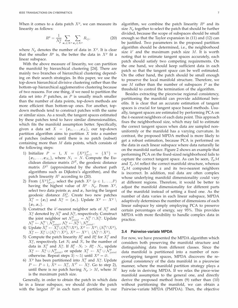
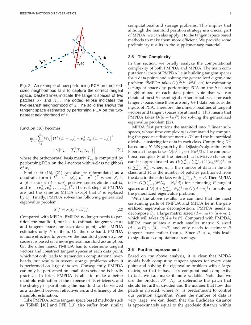
Besides extracting the piecewise regional consistency,partitioning the manifold can provide additional ben-efits. It is clear that an accurate estimation of tangentspaces is crucial for tangent space based methods. Usu-ally, tangent spaces are estimated by performing PCA onthe k-nearest neighbors of each data point. This approachfixes the neighborhood size, which may fail to estimatethe correct tangent spaces when data are sampled non-uniformly or the manifold has a varying curvature. Incontrast, the proposed MPDA method is more likely toget a robust estimation, because PCA is performed onthe data in each linear subspace where data naturally lieon the manifold surface. Figure 2 shows an example thatperforming PCA on the fixed-sized neighborhood fails tocapture the correct tangent space. As can be seen, TpMand Tp′M reflect the correct manifold structure, whereasTzM computed by z and its two-nearest neighborsis incorrect. In addition, real data are often complexwhose underlying manifold dimensionality could varyat different regions. Therefore, it would be better toadjust the manifold dimensionality for different partsof the manifold instead of setting a fixed one. As thenumber of data varies in each linear subspace, MPDAadaptively determines the number of dimensions of eachlinear subspace by simply employing PCA to preservecertain percentages of energy, say 95%. This providesMPDA with more flexibility to handle complex data inpractice.

3.4 Pairwise-variate MPDA

For now, we have presented the MPDA algorithm whichconsiders both preserving the manifold structure anddistinguishing data from different classes. Since thedata manifold is partitioned into a number of non-overlapping tangent spaces, MPDA discovers the re-gional consistency of the data manifold in a piecewisemanner, where the manifold partition strategy plays akey role in deriving MPDA. If we relax the piece-wisemanifold assumption to the general one, and directlyderive the proposed method from (9) rather than (10)without partitioning the manifold, we can obtain aPairwise-variate MPDA (PMPDA). Then, the objective


Fig. 2. An example of how performing PCA on the fixed-sized neighborhood fails to capture the correct tangentspace. Dashed lines indicate the tangent spaces of twopatches Xp and Xp′ . The dotted ellipse indicates thetwo-nearest neighborhood of z. The solid line shows thetangent space estimated by performing PCA on the two-nearest neighborhood of z.

function (16) becomes:

mint,v

n∑

i,j

Wij

[

(

t⊤(xi − xj)− v⊤xj

T⊤xj

(xi − xj))2

+ γ‖vxi− T⊤

xiTxj

vxj‖22

]

, (21)

where the orthonormal basis matrix Txiis computed by

performing PCA on the k-nearest within-class neighborsof xi.

Similar to (16), (21) can also be reformulated as aquadratic form ( t⊤ v⊤ )Sp( t⊤ v⊤ )⊤ where Sp isa (d + mn) × (d + mn) positive semi-definite matrix,and v = (v⊤

x1, v⊤

x2, . . . , v⊤

xn)⊤. The rest steps of PMPDA

are just the same as MPDA except that S is replacedby Sp. Finally, PMPDA solves the following generalizedeigenvalue problem:

S′f = λ(Sp + αI)f . (22)

Compared with MPDA, PMPDA no longer needs to par-tition the manifold, but has to estimate tangent vectorsand tangent spaces for each data point, while MPDAestimates only P of them. On the one hand, PMPDAis more effective to preserve the manifold geometry, be-cause it is based on a more general manifold assumption.On the other hand, PMPDA has to determine tangentvectors and construct tangent spaces at each data point,which not only leads to tremendous computational over-heads, but results in severe storage problems when itis performed on large data sets. Consequently, PMPDAcan only be performed on small data sets and is hardlypractical. In brief, PMPDA is able to make a bettermanifold estimation at the expense of its efficiency, andthe strategy of partitioning the manifold can be viewedas a trade-off between effectiveness and efficiency of themanifold estimation.

Like PMPDA, some tangent space based methods suchas TSIMR [10] and PFE [13] also suffer from similar

computational and storage problems. This implies thatalthough the manifold partition strategy is a crucial partof MPDA, we can also apply it to the tangent space basedmethods to make them more efficient. We provide somepreliminary results in the supplementary material.

3.5 Time Complexity

In this section, we briefly analyze the computationalcomplexity of both PMPDA and MPDA. The main com-putational costs of PMPDA lie in building tangent spacesfor n data points and solving the generalized eigenvalueproblem. PMPDA takes O((d2k+k2d)×n) for estimatingn tangent spaces by performing PCA on the k-nearestneighborhood of each data point. Note that we canobtain at most k meaningful orthonormal bases for eachtangent space, since there are only k+1 data points as theinputs of PCA. Therefore, the dimensionalities of tangentvectors and tangent spaces are at most k. This means thatPMPDA takes O((d + kn)3) for solving the generalizedeigenvalue problem (22).

MPDA first partitions the manifold into P linear sub-spaces, whose time complexity is dominated by comput-ing the geodesic distance matrix DG and the hierarchicaldivisive clustering for data in each class. Computing DG

based on a k′-NN graph by the Dijkstra’s algorithm withFibonacci heaps takes O(n2 log n+k′n2/2). The computa-tional complexity of the hierarchical divisive clustering

can be approximated as O(∑C

c=1

∑Pc

p=1(2p(nc/2p))2) ≈

O(∑C

c=1n2

c), where nc is the number of data in the c-thclass, and Pc is the number of patches partitioned from

the data in the c-th class with∑C

c=1Pc = P . Then MPDA

takes O(∑P

p=1(d2Np + Np

2d)) for estimating P tangent

spaces and O((d +∑P

p=1Np)

3) = O((d + n)3) for solvingthe generalized eigenvalue problem.

With the above results, we can find that the mostconsuming parts of PMPDA and MPDA lie in the gen-eralized eigenvalue decomposition. PMPDA needs todecompose Sp, a large matrix sized (d+mn)× (d+mn),which will takes O((d + kn)3). Compared with PMPDA,MPDA manipulates a much smaller matrix S sized(d + mP ) × (d + mP ) and only needs to estimate Ptangent spaces rather than n. Since P ≪ n, this leadsto significant computational savings.

3.6 Further Improvement

Based on the above analysis, it is clear that MPDAavoids both computing tangent spaces for every datapoint and solving the eigenvalue problem with a largematrix, so that it have less computational complexity.In fact, we can make it more scalable. Note that weuse the product Rp · Np to determine the patch thatshould be further divided and the manner that how thispatch is divided, where Np is predominant to controlour partition algorithm. When the number of data isvery large, we can deem that the Euclidean distanceis approximately equal to the geodesic distance within


a small region, which leads to Rp ≈ 1. Therefore, thepartition algorithm can be simplified by omitting thecomputation of DG and Rp, so that we can save the timefor performing Dijkstra’s algorithm and computing Rp.

In addition, the computational costs of MPDA canbe reduced by estimating tangent vectors and tangentspaces only at anchor points. In this case, we are inter-ested in selecting a portion of points from the originaldata set as the anchor points, and the rest can be rep-resented according to the first-order Taylor expansion attheir nearest anchor points. Therefore, the data manifoldcan be estimated by using the anchor points only. It isnatural to specify the center of each linear subspaces,which is not necessary a data point among the trainingset, as the anchor point. As a result, MPDA can beperformed on only P anchor points rather than thewhole data set, such that the corresponding computa-tional complexity for solving the generalized eigenvalueproblem can be reduced to O((d + P )3).

Moreover, the two-stage strategy [25] can be adoptedto further reduce the computational costs. We can sep-arate the generalized eigenvalue problem (19) into twostages. The first stage maximizes (17) via QR decomposi-tion to find its solution space. The second one solves (19)in the solution space of (17). Since S′ is just the extensionof 2XL′X⊤, the rank of S′ is at most d. Consequently,the time for solving (19) can be reduced to O(d3). Pleaserefer to [25] for more details.

4 DISCUSSION

Several works have been done to manipulate data inlocal subspaces for dimensionality reduction [26], [27],[28], [29]. Basically, they share the same spirit in aligninglocal subspaces to build a global coordinate, where theconnections of local subspaces are considered implicitly.The main difference between MPDA and these methodsis that MPDA constructs tangent spaces in a piecewisemanner and explicitly characterizes their connections byestimating tangent vectors.

Local Linear Coordination (LLC) [26] and CoordinatedFactor Analysis (CFA) [27] construct linear subspacesthrough the mixture of factor analyzers (MFA) which canserve as an alternative way to partition the data mani-fold. However, MFA is optimized by the expectation-maximization (EM) algorithm, which can be slow andunstable. Moreover, the number of factor analyzers andthe dimensionality of each linear subspace should bespecified as a priori knowledge, which are difficult todetermine. In contrast, the proposed manifold partitionalgorithm for constructing linear subspaces is more ef-ficient, and the dimensionality of each linear subspacecan be determined automatically by using PCA.

Compared with MPDA, Maximal Linear Embedding(MLE) [29] also constructs a number of linear subspacesbased on the measure of linearity but follows a differentprinciple. MLE prefers to construct the linear subspaceswhose sizes should be as large as possible, while MPDA

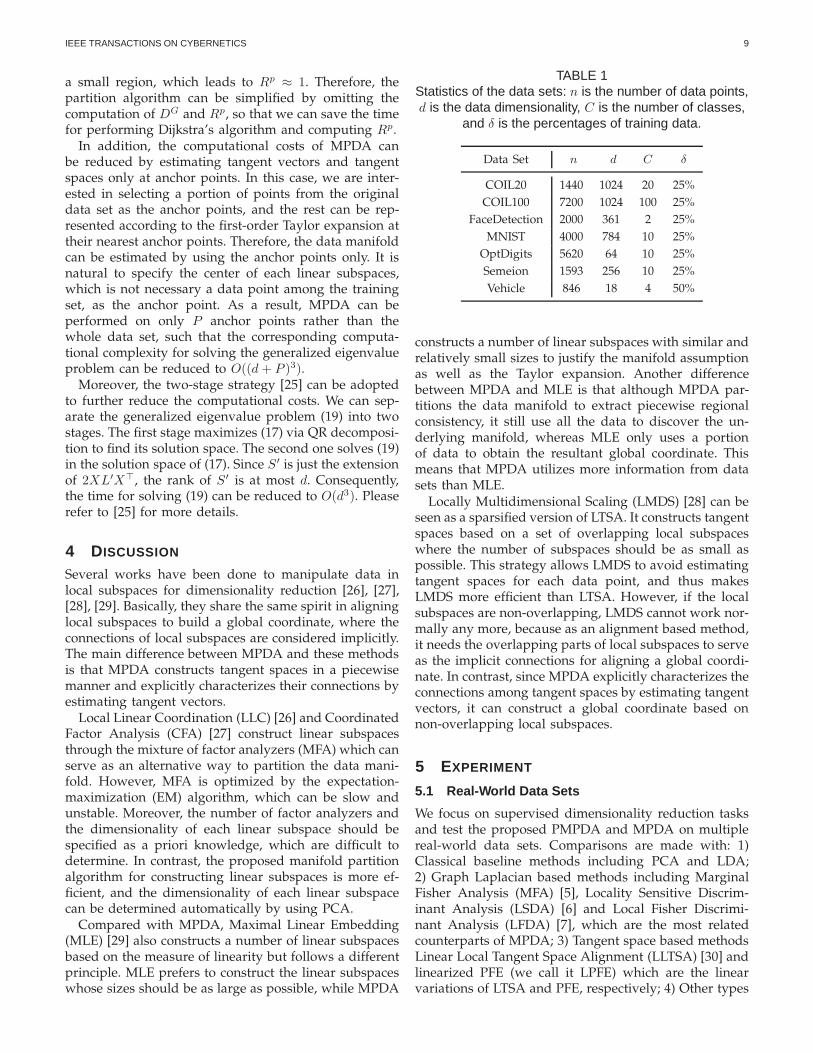
TABLE 1Statistics of the data sets: n is the number of data points,d is the data dimensionality, C is the number of classes,

and δ is the percentages of training data.

Data Set n d C δ

COIL20 1440 1024 20 25%

COIL100 7200 1024 100 25%

FaceDetection 2000 361 2 25%

MNIST 4000 784 10 25%

OptDigits 5620 64 10 25%

Semeion 1593 256 10 25%

Vehicle 846 18 4 50%

constructs a number of linear subspaces with similar andrelatively small sizes to justify the manifold assumptionas well as the Taylor expansion. Another differencebetween MPDA and MLE is that although MPDA par-titions the data manifold to extract piecewise regionalconsistency, it still use all the data to discover the un-derlying manifold, whereas MLE only uses a portionof data to obtain the resultant global coordinate. Thismeans that MPDA utilizes more information from datasets than MLE.

Locally Multidimensional Scaling (LMDS) [28] can beseen as a sparsified version of LTSA. It constructs tangentspaces based on a set of overlapping local subspaceswhere the number of subspaces should be as small aspossible. This strategy allows LMDS to avoid estimatingtangent spaces for each data point, and thus makesLMDS more efficient than LTSA. However, if the localsubspaces are non-overlapping, LMDS cannot work nor-mally any more, because as an alignment based method,it needs the overlapping parts of local subspaces to serveas the implicit connections for aligning a global coordi-nate. In contrast, since MPDA explicitly characterizes theconnections among tangent spaces by estimating tangentvectors, it can construct a global coordinate based onnon-overlapping local subspaces.

5 EXPERIMENT

5.1 Real-World Data Sets

We focus on supervised dimensionality reduction tasksand test the proposed PMPDA and MPDA on multiplereal-world data sets. Comparisons are made with: 1)Classical baseline methods including PCA and LDA;2) Graph Laplacian based methods including MarginalFisher Analysis (MFA) [5], Locality Sensitive Discrim-inant Analysis (LSDA) [6] and Local Fisher Discrimi-nant Analysis (LFDA) [7], which are the most relatedcounterparts of MPDA; 3) Tangent space based methodsLinear Local Tangent Space Alignment (LLTSA) [30] andlinearized PFE (we call it LPFE) which are the linearvariations of LTSA and PFE, respectively; 4) Other types


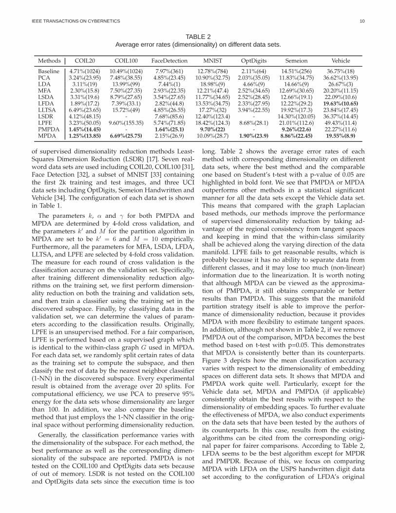
TABLE 2Average error rates (dimensionality) on different data sets.

Methods COIL20 COIL100 FaceDetection MNIST OptDigits Semeion Vehicle

Baseline 4.71%(1024) 10.49%(1024) 7.97%(361) 12.78%(784) 2.11%(64) 14.51%(256) 36.75%(18)PCA 3.24%(23.95) 7.48%(38.55) 4.85%(23.45) 10.90%(32.75) 2.03%(35.05) 11.83%(34.75) 36.62%(13.95)LDA 3.11%(19) 13.99%(99) 7.44%(1) 18.98%(9) 4.66%(9) 14.66%(9) 26.67%(3)MFA 2.30%(15.8) 7.50%(27.35) 2.93%(22.35) 12.21%(47.4) 2.52%(34.65) 12.69%(30.65) 20.20%(11.15)LSDA 3.31%(19.6) 8.79%(27.65) 3.54%(27.65) 11.77%(34.65) 2.52%(28.45) 12.66%(19.1) 22.09%(10.6)LFDA 1.89%(17.2) 7.39%(33.1) 2.82%(44.8) 13.53%(34.75) 2.33%(27.95) 12.22%(29.2) 19.63%(10.65)LLTSA 6.49%(23.65) 15.72%(49) 4.85%(26.55) 17.27%(32) 3.94%(22.55) 19.92%(17.3) 23.84%(17.45)LSDR 4.12%(48.15) - 7.68%(85.6) 12.40%(123.4) - 14.30%(120.05) 36.37%(14.45)LPFE 3.23%(50.05) 9.60%(155.35) 5.74%(71.85) 18.42%(124.3) 8.68%(28.1) 21.01%(112.6) 49.43%(11.4)PMPDA 1.45%(14.45) - 1.64%(25.1) 9.70%(22) - 9.26%(22.6) 22.27%(11.6)MPDA 1.25%(13.85) 6.69%(25.75) 2.15%(26.9) 10.09%(28.7) 1.90%(23.9) 8.86%(22.45) 19.55%(8.9)

of supervised dimensionality reduction methods Least-Squares Dimension Reduction (LSDR) [17]. Seven real-word data sets are used including COIL20, COIL100 [31],Face Detection [32], a subset of MNIST [33] containingthe first 2k training and test images, and three UCIdata sets including OptDigits, Semeion Handwritten andVehicle [34]. The configuration of each data set is shownin Table 1.

The parameters k, α and γ for both PMPDA andMPDA are determined by 4-fold cross validation, andthe parameters k′ and M for the partition algorithm inMPDA are set to be k′ = 6 and M = 10 empirically.Furthermore, all the parameters for MFA, LSDA, LFDA,LLTSA, and LPFE are selected by 4-fold cross validation.The measure for each round of cross validation is theclassification accuracy on the validation set. Specifically,after training different dimensionality reduction algo-rithms on the training set, we first perform dimension-ality reduction on both the training and validation sets,and then train a classifier using the training set in thediscovered subspace. Finally, by classifying data in thevalidation set, we can determine the values of param-eters according to the classification results. Originally,LPFE is an unsupervised method. For a fair comparison,LPFE is performed based on a supervised graph whichis identical to the within-class graph G used in MPDA.For each data set, we randomly split certain rates of dataas the training set to compute the subspace, and thenclassify the rest of data by the nearest neighbor classifier(1-NN) in the discovered subspace. Every experimentalresult is obtained from the average over 20 splits. Forcomputational efficiency, we use PCA to preserve 95%energy for the data sets whose dimensionality are largerthan 100. In addition, we also compare the baselinemethod that just employs the 1-NN classifier in the orig-inal space without performing dimensionality reduction.

Generally, the classification performance varies withthe dimensionality of the subspace. For each method, thebest performance as well as the corresponding dimen-sionality of the subspace are reported. PMPDA is nottested on the COIL100 and OptDigits data sets becauseof out of memory. LSDR is not tested on the COIL100and OptDigits data sets since the execution time is too

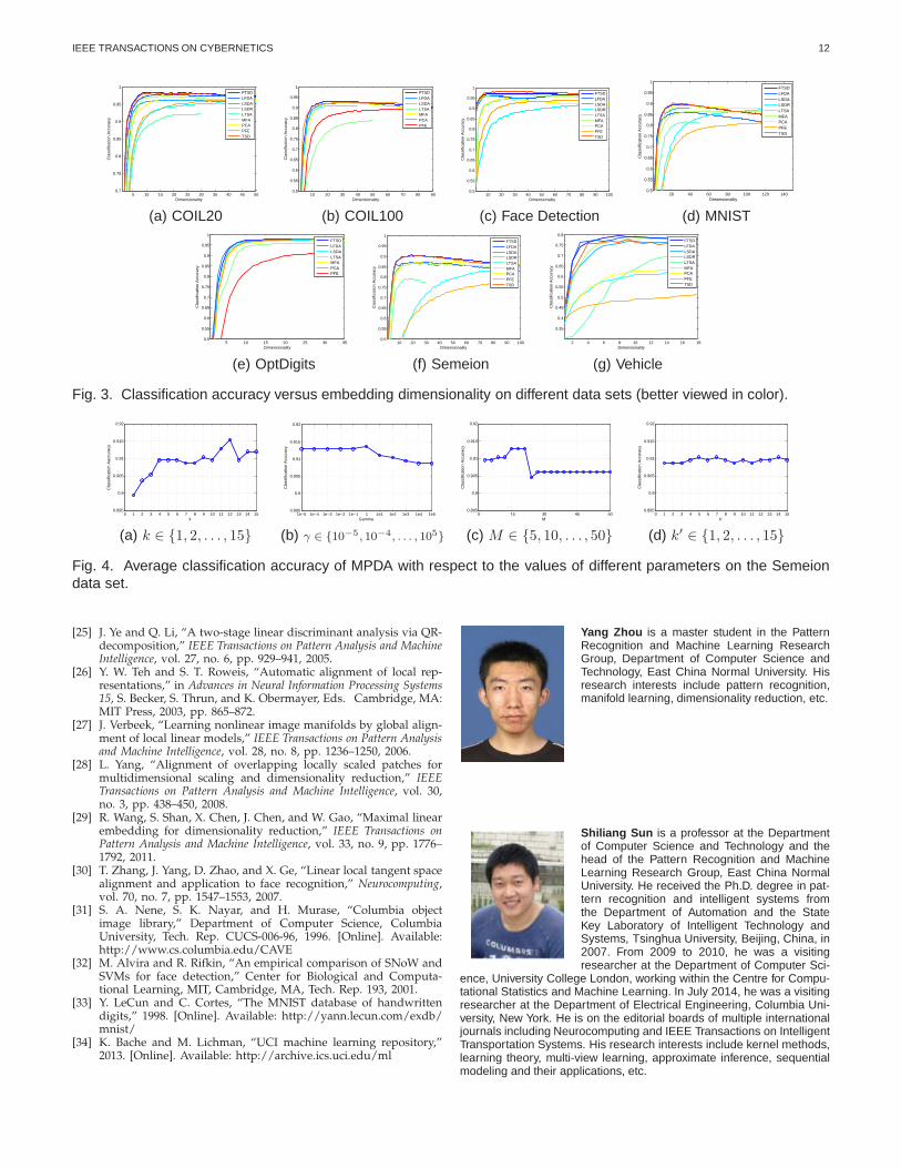
long. Table 2 shows the average error rates of eachmethod with corresponding dimensionality on differentdata sets, where the best method and the comparableone based on Student’s t-test with a p-value of 0.05 arehighlighted in bold font. We see that PMPDA or MPDAoutperforms other methods in a statistical significantmanner for all the data sets except the Vehicle data set.This means that compared with the graph Laplacianbased methods, our methods improve the performanceof supervised dimensionality reduction by taking ad-vantage of the regional consistency from tangent spacesand keeping in mind that the within-class similarityshall be achieved along the varying direction of the datamanifold. LPFE fails to get reasonable results, which isprobably because it has no ability to separate data fromdifferent classes, and it may lose too much (non-linear)information due to the linearization. It is worth notingthat although MPDA can be viewed as the approxima-tion of PMPDA, it still obtains comparable or betterresults than PMPDA. This suggests that the manifoldpartition strategy itself is able to improve the perfor-mance of dimensionality reduction, because it providesMPDA with more flexibility to estimate tangent spaces.In addition, although not shown in Table 2, if we removePMPDA out of the comparison, MPDA becomes the bestmethod based on t-test with p=0.05. This demonstratesthat MPDA is consistently better than its counterparts.Figure 3 depicts how the mean classification accuracyvaries with respect to the dimensionality of embeddingspaces on different data sets. It shows that MPDA andPMPDA work quite well. Particularly, except for theVehicle data set, MPDA and PMPDA (if applicable)consistently obtain the best results with respect to thedimensionality of embedding spaces. To further evaluatethe effectiveness of MPDA, we also conduct experimentson the data sets that have been tested by the authors ofits counterparts. In this case, results from the existingalgorithms can be cited from the corresponding origi-nal paper for fairer comparisons. According to Table 2,LFDA seems to be the best algorithm except for MPDRand PMPDR. Because of this, we focus on comparingMPDA with LFDA on the USPS handwritten digit dataset according to the configuration of LFDA’s original


paper. Again, MPDR and PMPDR outperform theircounterparts with statistical significance. Please refer tothe supplementary material for details.

5.2 Parameter Sensitivity

In this section, we evaluate the parameter sensitivity ofMPDA on the Semeion Handwritten data set. Specifi-cally, we aim to test how the performance of MPDAvaries with its parameters k, γ, M , and k′, respectively.To this end, the default values of k, γ, M and k′ are set tobe 5, 1, 10 and 6, respectively. And we alternately changeone of these parameters to evaluate the performance ofMPDA when the other parameters are fixed. Figure 4implies that k and M are more important than γ andk′. Their values should be determined properly, whilethose of γ and k′ seem to have no significant influenceon the performance of MPDA. Overall, MPDA get stableresults as its parameters change, where the classificationaccuracy ranges from 90% to 92%. Therefore, MPDA isrelatively insensitive to the changes of parameters.

6 CONCLUSION

In this paper we have proposed a tangent space basedlinear dimensionality reduction method named ManifoldPartition Discriminant Analysis (MPDA). By consideringboth pairwise differences and piecewise regional consis-tency, MPDA can find a linear embedding space wherethe within-class similarity is achieved along the directionthat is consistent with the local variation of the data man-ifold, while nearby data belonging to different classesare well separated. Different to graph Laplacian methodsthat capture only the pairwise interaction between datapoints, our method capture both pairwise as well ashigher order interactions (using regional consistency)between data points.

As a crucial part of MPDA, the manifold partitionstrategy plays a key role in preserving the manifoldstructure to improve the measure of the within-classsimilarity. It not only enables MPDA to adaptively deter-mine the number of dimensions of each linear subspace,but also can be adopted by other tangent space basemethods to make them more efficient. The experimentson multiple real-world data sets have shown that com-pared with existing works MPDA can obtain betterclassification results.

ACKNOWLEDGMENTS

This work is supported by the National Natural Sci-ence Foundation of China under Projects 61370175,and Shanghai Knowledge Service Platform Project (No.ZF1213).

REFERENCES

[1] D. Q. Dai and P. C. Yuen, “Face recognition by regularizeddiscriminant analysis,” IEEE Transactions on Systems, Man, andCybernetics, Part B: Cybernetics, vol. 37, no. 4, pp. 1080–1085, 2007.

[2] H. Zhao and P. C. Yuen, “Incremental linear discriminant analysisfor face recognition,” IEEE Transactions on Systems, Man, andCybernetics, Part B: Cybernetics, vol. 38, no. 1, pp. 210–221, 2008.

[3] F. Dornaika and A. Bosaghzadeh, “Exponential local discriminantembedding and its application to face recognition,” IEEE Transac-tions on Cybernetics, vol. 43, no. 3, pp. 921–934, 2013.

[4] H. Wang, X. Lu, Z. Hu, and W. Zheng, “Fisher discriminantanalysis with L1-norm,” IEEE Transactions on Cybernetics, vol. 44,no. 6, pp. 828–841, 2014.

[5] S. Yan, D. Xu, B. Zhang, H. Zhang, Q. Yang, and S. Lin, “Graphembedding and extensions: a general framework for dimension-ality reduction,” IEEE Transactions on Pattern Analysis and MachineIntelligence, vol. 29, no. 1, pp. 40–51, 2007.

[6] D. Cai, X. He, K. Zhou, J. Han, and H. Bao, “Locality sensitivediscriminant analysis,” in Proceedings of the 20th International JointConference on Artificial Intelligence, 2007, pp. 708–713.

[7] M. Sugiyama, “Dimensionality reduction of multimodal labeleddata by local Fisher discriminant analysis,” Journal of MachineLearning Research, vol. 8, pp. 1027–1061, 2007.

[8] S. Pedagadi, J. Orwell, S. Velastin, and B. Boghossian, “Localfisher discriminant analysis for pedestrian re-identification,” inProceedings of IEEE Conference on Computer Vision and PatternRecognition, 2013, pp. 3318–3325.

[9] P. Simard, Y. LeCun, and J. S. Denker, “Efficient pattern recogni-tion using a new transformation distance,” S. Hanson, J. Cowan,and C. Giles, Eds. Cambridge, MA: Morgan-Kaufmann, 1993,pp. 50–58.

[10] S. Sun, “Tangent space intrinsic manifold regularization for datarepresentation,” in Proceedings of the IEEE China Summit andInternational Conference on Signal and Information Processing, 2013,pp. 179–183.

[11] Z. Zhang and H. Zha, “Principal manifolds and nonlinear dimen-sion reduction via local tangent space alignment,” SIAM Journalon Scientific Computing, vol. 26, no. 1, pp. 313–338, 2004.

[12] M. Brand, “Charting a manifold,” in Advances in Neural Informa-tion Processing Systems 15, S. Becker, S. Thrun, and K. Obermayer,Eds. Cambridge, MA: MIT Press, 2003, pp. 985–992.

[13] B. Lin, X. He, C. Zhang, and M. Ji, “Parallel vector field em-bedding,” Journal of Machine Learning Research, vol. 14, no. 1, pp.2945–2977, 2013.

[14] D. Huang, M. Storer, F. De la Torre, and H. Bischof, “Supervisedlocal subspace learning for continuous head pose estimation,”in Proceedings of IEEE Conference on Computer Vision and PatternRecognition, 2011, pp. 2921–2928.

[15] H. Tang, S. M. Chu, M. Hasegawa-Johnson, and T. S. Huang,“Partially supervised speaker clustering,” IEEE Transactions onPattern Analysis and Machine Intelligence, vol. 34, no. 5, pp. 959–971,2012.

[16] T. Zhou and D. Tao, “Double shrinking sparse dimension reduc-tion,” IEEE Transactions on Image Processing, vol. 22, no. 1, pp.244–257, 2013.

[17] T. Suzuki and M. Sugiyama, “Sufficient dimension reduction viasquared-loss mutual information estimation,” Neural Computation,vol. 25, no. 3, pp. 725–758, 2013.

[18] S. Wang, S. Yan, J. Yang, C. Zhou, and X. Fu, “A general exponen-tial framework for dimensionality reduction,” IEEE Transactions onImage Processing, vol. 23, no. 2, pp. 920–930, 2014.

[19] F. R. K. Chung, Spectral Graph Theory. Rhode Island: AmericanMathematical Society, 1997.

[20] K. Fukunaga, Introduction to Statistical Pattern Recognition, 2nd ed.Academic Press, 1990.

[21] P. Y. Simard, Y. A. LeCun, J. S. Denker, and B. Victorri, “Transfor-mation invariance in pattern recognition–Tangent distance andtangent propagation,” in Neural Networks: Tricks of the Trade.Springer, 2012, vol. 7700, pp. 235–269.

[22] W. Min, K. Lu, and X. He, “Locality pursuit embedding,” PatternRecognition, vol. 37, no. 4, pp. 781–788, 2004.

[23] M. B. Clennell, “Tortuosity: A guide through the maze,” GeologicalSociety Special Publications, vol. 122, pp. 299–344, 1997.

[24] L. Kaufman and P. J. Rousseeuw, Finding Groups in Data: AnIntroduction to Cluster Analysis. John Wiley & Sons, 2009.


5 10 15 20 25 30 35 40 45 500.7

0.75

0.8

0.85

0.9

0.95

1

Dimensionality

Cla

ssifi

catio

n A

ccur

acy

FTSDLFDALSDALSDRLTSAMFAPCAPFETSD

(a) COIL20

10 20 30 40 50 60 70 80 900.5

0.55

0.6

0.65

0.7

0.75

0.8

0.85

0.9

0.95

1

Dimensionality

Cla

ssifi

catio

n A

ccur

acy

FTSDLFDALSDALTSAMFAPCAPFE

(b) COIL100

10 20 30 40 50 60 70 80 90 1000.5

0.55

0.6

0.65

0.7

0.75

0.8

0.85

0.9

0.95

1

Dimensionality

Cla

ssifi

catio

n A

ccur

acy


(c) Face Detection

20 40 60 80 100 120 1400.5

0.55

0.6

0.65

0.7

0.75

0.8

0.85

0.9

0.95

1

Dimensionality

Cla

ssifi

catio

n A

ccur

acy


(d) MNIST

5 10 15 20 25 30 350.5

0.55

0.6

0.65

0.7

0.75

0.8

0.85

0.9

0.95

1

Dimensionality

Cla

ssifi

catio

n A

ccur

acy

FTSDLFDALSDALTSAMFAPCAPFE

(e) OptDigits

10 20 30 40 50 60 70 80 90 1000.5

0.55

0.6

0.65

0.7

0.75

0.8

0.85

0.9

0.95

1

Dimensionality

Cla

ssifi

catio

n A

ccur

acy


(f) Semeion

2 4 6 8 10 12 14 16 18

0.35

0.4

0.45

0.5

0.55

0.6

0.65

0.7

0.75

0.8

Dimensionality

Cla

ssifi

catio

n A

ccur

acy


(g) Vehicle

Fig. 3. Classification accuracy versus embedding dimensionality on different data sets (better viewed in color).

0 1 2 3 4 5 6 7 8 9 10 11 12 13 14 150.895

0.9

0.905

0.91

0.915

0.92

k

Cla

ssifi

catio

n A

accu

racy

(a) k ∈ {1, 2, . . . , 15}

1e−5 1e−4 1e−3 1e−2 1e−1 1 1e1 1e2 1e3 1e4 1e50.895

0.9

0.905

0.91

0.915

0.92

Gamma

Cla

ssifi

catio

n A

ccur

acy

(b) γ ∈ {10−5, 10

−4, . . . , 10

5}

0 00.895

0.9

0.905

0.91

0.915

0.92

M

Cla

ssifi

catio

n A

ccur

acy

(c) M ∈ {5, 10, . . . , 50}

0 1 2 3 4 5 6 7 8 9 10 11 12 13 14 150.895

0.9

0.905

0.91

0.915

0.92

k’

Cla

ssifi

catio

n A

ccur

acy

(d) k′ ∈ {1, 2, . . . , 15}

Fig. 4. Average classification accuracy of MPDA with respect to the values of different parameters on the Semeiondata set.

[25] J. Ye and Q. Li, “A two-stage linear discriminant analysis via QR-decomposition,” IEEE Transactions on Pattern Analysis and MachineIntelligence, vol. 27, no. 6, pp. 929–941, 2005.

[26] Y. W. Teh and S. T. Roweis, “Automatic alignment of local rep-resentations,” in Advances in Neural Information Processing Systems15, S. Becker, S. Thrun, and K. Obermayer, Eds. Cambridge, MA:MIT Press, 2003, pp. 865–872.

[27] J. Verbeek, “Learning nonlinear image manifolds by global align-ment of local linear models,” IEEE Transactions on Pattern Analysisand Machine Intelligence, vol. 28, no. 8, pp. 1236–1250, 2006.

[28] L. Yang, “Alignment of overlapping locally scaled patches formultidimensional scaling and dimensionality reduction,” IEEETransactions on Pattern Analysis and Machine Intelligence, vol. 30,no. 3, pp. 438–450, 2008.

[29] R. Wang, S. Shan, X. Chen, J. Chen, and W. Gao, “Maximal linearembedding for dimensionality reduction,” IEEE Transactions onPattern Analysis and Machine Intelligence, vol. 33, no. 9, pp. 1776–1792, 2011.

[30] T. Zhang, J. Yang, D. Zhao, and X. Ge, “Linear local tangent spacealignment and application to face recognition,” Neurocomputing,vol. 70, no. 7, pp. 1547–1553, 2007.

[31] S. A. Nene, S. K. Nayar, and H. Murase, “Columbia objectimage library,” Department of Computer Science, ColumbiaUniversity, Tech. Rep. CUCS-006-96, 1996. [Online]. Available:http://www.cs.columbia.edu/CAVE

[32] M. Alvira and R. Rifkin, “An empirical comparison of SNoW andSVMs for face detection,” Center for Biological and Computa-tional Learning, MIT, Cambridge, MA, Tech. Rep. 193, 2001.

[33] Y. LeCun and C. Cortes, “The MNIST database of handwrittendigits,” 1998. [Online]. Available: http://yann.lecun.com/exdb/mnist/

[34] K. Bache and M. Lichman, “UCI machine learning repository,”2013. [Online]. Available: http://archive.ics.uci.edu/ml

Yang Zhou is a master student in the PatternRecognition and Machine Learning ResearchGroup, Department of Computer Science andTechnology, East China Normal University. Hisresearch interests include pattern recognition,manifold learning, dimensionality reduction, etc.

Shiliang Sun is a professor at the Departmentof Computer Science and Technology and thehead of the Pattern Recognition and MachineLearning Research Group, East China NormalUniversity. He received the Ph.D. degree in pat-tern recognition and intelligent systems fromthe Department of Automation and the StateKey Laboratory of Intelligent Technology andSystems, Tsinghua University, Beijing, China, in2007. From 2009 to 2010, he was a visitingresearcher at the Department of Computer Sci-

ence, University College London, working within the Centre for Compu-tational Statistics and Machine Learning. In July 2014, he was a visitingresearcher at the Department of Electrical Engineering, Columbia Uni-versity, New York. He is on the editorial boards of multiple internationaljournals including Neurocomputing and IEEE Transactions on IntelligentTransportation Systems. His research interests include kernel methods,learning theory, multi-view learning, approximate inference, sequentialmodeling and their applications, etc.

1

Supplementary Material for Manifold PartitionDiscriminant Analysis

Yang Zhou and Shiliang Sun

✦

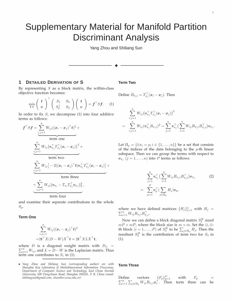
1 DETAILED DERIVATION OF SBy representing S as a block matrix, the within-classobjective function becomes:

mint,v

(

t

v

)⊤(

S1 S2

S⊤2

S3

)(

t

v

)

= f⊤Sf . (1)

In order to fix S, we decompose (1) into four additiveterms as follows:

f⊤Sf =

n∑

i,j=1

Wij((xi − xj)⊤t)2

︸︷︷︸

term one

+

n∑

i,j=1

Wij

(

v⊤πj

T⊤πj

(xi − xj))2

︸︷︷︸

term two

+

n∑

i,j=1

Wij

[

− 2((xi − xj)⊤t)v⊤

πjT⊤

πj(xi − xj)

]

︸︷︷︸

term three

+

γ

n∑

i,j=1

Wij‖vπi− Tπi

T⊤πj

vπj‖2

2

︸︷︷︸

term four

,

and examine their separate contributions to the wholeSp.

Term One

n∑

i,j=1

Wij((xi − xj)⊤t)2

=2t⊤X(D − W )X⊤t = 2t⊤XLX⊤t,

where D is a diagonal weight matrix with Dii =∑n

j=1Wij , and L = D−W is the Laplacian matrix. Thus

term one contributes to S1 in (1).

• Yang Zhou and Shiliang Sun (corresponding author) are withShanghai Key Laboratory of Multidimensional Information Processing,Department of Computer Science and Technology, East China NormalUniversity, 500 Dongchuan Road, Shanghai 200241, P. R. China (email:[email protected], [email protected])

Term Two

Define Bπji = T⊤πj

(xi − xj). Then

n∑

i,j=1

Wij

(

v⊤πj

T⊤πj

(xi − xj))2

=

n∑

i,j=1

Wij(v⊤πj

Bπji)2 =

n∑

j=1

v⊤πj

(

n∑

i=1

WijBπjiB⊤πji

)

vπj.

Let Πp = {i|πi = p, i ∈ {1, . . . , n}} be a set that consistsof the indices of the data belonging to the p-th linearsubspace. Then we can group the terms with respect tovπj

(j = 1, . . . , n) into P terms as follows:

n∑

j=1

v⊤πj

(

n∑

i=1

WijBπjiB⊤πji

)

vπj(2)

=

P∑

p=1

v⊤p (∑

j∈Πp

Hj)vp,

where we have defined matrices {Hj}nj=1

with Hj =∑n

i=1WijBπjiB

⊤πji.

Now we can define a block diagonal matrix SH3

sizedmP × mP , where the block size is m × m. Set the (i, i)-th block (i = 1, . . . , P ) of SH

3to be

∑

j∈ΠpHj . Then the

resultant SH3

is the contribution of term two for S3 in(1).

Term Three

Define vectors {Fp}Pp=1

with Fp =∑n

i=1

∑

j∈ΠpWijBπjix

⊤i . Then term three can be

2

rewritten as:n∑

i,j=1

Wij

[

− 2((xi − xj)⊤t)v⊤

πjT⊤

πj(xi − xj)

]

=

n∑

i,j=1

2Wij

[

((xj − xi)⊤t)v⊤

πjBπji

]

=P∑

p=1

t⊤(n∑

i=1

∑

j∈Πp

−WijxiB⊤πji)vp +

P∑

p=1

v⊤p (

n∑

i=1

∑

j∈Πp

−WijBπjix⊤i )t +

P∑

p=1

t⊤F⊤p vp +

P∑

p=1

v⊤p Fpt.

From this expression, we can give the formulation of S2.Then the block matrix S⊤

2in (1), which is its transpose,

is ready to get.Suppose we define two block matrices S1

2and S2

2sized

d × mP each where the block size is d × m, and S2

2is a

block diagonal matrix. Set the p-th block (p = 1, . . . , P )of S1

2to be

∑n

i=1

∑

j∈Πp−WijxiB

⊤πji, and the (p, p)-th

block (p = 1, . . . , P ) of S2

2to be F⊤

p . Then, term threecan be rewritten as: t⊤(S1

2+ S2

2)v + v⊤(S1

2+ S2

2)⊤t. It is

clear that S2 = S1

2+ S2

2.

Term Four

Denote matrix TπiT⊤

πjby Aπiπj

. Then, with γ omittedtemporarily,

n∑

i,j=1

Wij‖vπi− Tπi

T⊤πj

vπj‖2

2

=

n∑

i,j=1

Wijv⊤πj

A⊤πiπj

Aπiπjvπj

+

n∑

i,j=1

Wijv⊤πi

vπi−

n∑

i,j=1

2Wijv⊤πi

Aπiπjvπj

.

Similarly, we can sum up the terms with respect to vπj,

which further leads to:n∑

i,j=1

Wijv⊤πj

A⊤πiπj

Aπiπjvπj

+

n∑

i=1

Diiv⊤πi

Ivπi−

n∑

i,j=1

2Wijv⊤πi

Aπiπjvπj

=

P∑

p=1

v⊤p (∑

j∈Πp

(DjjI + Cj))vp −

P∑

p=1

P∑

q=1

v⊤p (∑

i∈Πp

∑

j∈Πq

2WijAπiπj)vq.

where in the third line we have defined matrices {Cj}nj=1

with Cj =∑n

i=1WijA

⊤πiπj

Aπiπj.

Now suppose we define two block matrices S1

3and

S2

3sized mP × mP each where the block size is m× m,

TABLE 1Average error rates (dimensionality) on the USPS data

sets.

Methods USPS-eo USPS-sl

Baseline 2.72%(256) 3.25%(256)PCA 2.47%(37.9) 2.93%(38.75)LDA 10.93%(9) 21.25%(9)MFA 2.79%(26.3) 3.57%(29.45)LSDA 3.39%(26.8) 4.21%(27.1)LFDA 7.89%(39.25) 9.84%(20.9)LLTSA 8.16%(28.4) 8.47%(29.85)LSDR - -LPFE 4.33%(184.4) 3.61%(180.25)PMPDA 1.76%(28.65) 2.20%(31.6)MPDA 1.67%(35.25) 2.28%(30.2)

and S1

3is a block diagonal matrix. Set the (p, p)-th

block (p = 1, . . . , P ) of S1

3to be

∑

j∈Πp(DjjI + Cj),

and the (p, q)-th block (p, q = 1, . . . , P ) of S2

3to be

∑

i∈Πp

∑

j∈Πq2WijAπiπj

. Then the contribution of term

four for S3 would be γ(S1

3− S2

3). Further considering

the contribution of term two for S3, we finally haveS3 = SH

3+ γ(S1

3− S2

3).

2 USPS DATA SET

In this section, we further evaluate the effectiveness ofMPDA by conducting experiments on the data sets thathave been tested by the authors of its counterparts. Inthis case, results from the existing algorithms can becited from the corresponding original paper for fairercomparisons. According to Table 2 in our paper, LFDAseems to be the best algorithm except for MPDR andPMPDR. Because of this, we focus on comparing MPDAwith LFDA. Specifically, our experiments are conductedon two binary classification data sets created from theUSPS handwritten digit data set. The first task (USPS-eo)is to separate even numbers from odd numbers, and thesecond task (USPS-sl) is to separate small numbers (“0”to “4”) from large numbers (“5” to “9”). We randomlychose 100 data points from each digit to form both thetraining and test set, so that there are 1000 data points fortraining and testing, respectively. The strategy of modelselection is the same as that in our paper. We report thebest classification results obtained by each method andthe corresponding dimensionality at which the resultsare achieved. Every experimental result is obtained fromthe average over 20 times, where the best method andthe comparable one based on Student’s t-test with a p-value of 0.05 are highlighted in bold font. The aboveexperimental configuration is identical to the one usedin LFDAs original paper [1] except for two differences.The first is that the neighborhood size k is treated as aparameter for graph construction. We determine k via 4-fold cross validation, while k is set to be 7 in LFDA’soriginal paper [1]. The second is that we search allthe possible dimensionalities of embedding subspaces toreport the best classification results, whereas the results

3

Swiss roll

(a) Swiss roll (b) Sampled data

(c) TSIMR (27.64s) (d) MP-TSIMR (9.82s)

(e) LTSIMR (27.92s) (f) MP-LTSIMR (10.02s)

Fig. 1. The “Swiss roll” manifold and the correspondingembedding results (time) obtained by the dimensionalityreduction methods with and without partitioning the man-ifold.

in [1] are obtained by selecting the dimensionality of em-bedding subspaces via 20-fold cross validation. This twodifferences imply that we are expected to get relativelybetter results than those reported in [1]. Table 1 showsthat MPDA and PMPAD still outperform its counterpartswith statistical significance. LSDR is not tested since theexecution time is too long. It is worth noting that thereported classification results of LFDA in [1] are 9.0%for UPSP-eo and 12.9% for UPSP-sl, respectively. In ourexperiments, these results are improved as expected.However, they are still much worse than the results ofMPDA and PMPDA.

3 EFFECTIVENESS OF PARTITIONING THEMANIFOLD

As a crucial part of MPDA, the manifold partition strat-egy plays a key role in preserving the manifold structurewith computational and storage efficiency. In fact, it canalso be adopted by other tangent space base methods [2],[3] to make them more efficient. To verify its effective-ness, we apply the manifold partition strategy to TangentSpace Intrinsic Manifold Regularization (TSIMR) [3] andits linear variation (we call it LTSIMR). This further leadsto two algorithms called MP-TSIMR and MP-LTSIMR,which can be viewed as the approximated versions ofTSIMR and LTSIMR. To show the effectiveness of themanifold partition strategy, we compare the embeddingresults of these methods on the “Swiss roll” manifold.

The “Swiss roll” is a two-dimensional manifold ina three-dimensional ambient space as shown in Fig-ure 1(a). The data set consists of 2000 points sampledfrom the manifold, which are depicted in Figure 1(b).The construction of the adjacency graph uses 10 nearestneighbors with the heat kernel. The parameter t ofthe heat kernel is fixed as the average of the squareddistances between all points and their most nearest

neighbors. The parameter γ is set to be γ = 0 for TSIMRand MP-TSIMR, and γ = 109 for LTSIMR and MP-LTSIMR. We fix the parameters k′ = 31 and M = 48for the manifold partitioning algorithm.

Figure 1 shows the two-dimensional embedding re-sults obtained by different algorithms. As can be seen inFigure 1(c), TSIMR precisely reflects the intrinsic man-ifold structure. In addtion, Figure 1(d) shows that MP-TSIMR also gets a good embedding result besides a littledistortion. In the case of linear dimensionality reduction,LTSIMR and MP-LTSIMR almost get identical resultsas shown in Figures 1(e) and 1(f). These embeddingresults demonstrate that MP-TSIMR and MP-LTSIMRhave similar or the same embedding performance com-pared with TSIMR and LTSIMR. When it comes to thecomputational time, MP-TSIMR and MP-LTSIMR arethree times faster than their counterparts. This is becauseboth TSIMR and LTSIMR estimate 2000 tangent vectorsand tangent spaces to discover the intrinsic manifoldstructure, whereas MP-TSIMR and MP-LTSIMR onlyneed to estimate 65 tangent vectors and tangent spaces.Therefore, it is clear that the manifold partition strategynot only is useful for MPDA, but can accelerate othertangent space based methods without sacrificing theirperformances much.

4 STORAGE OVERHEADS

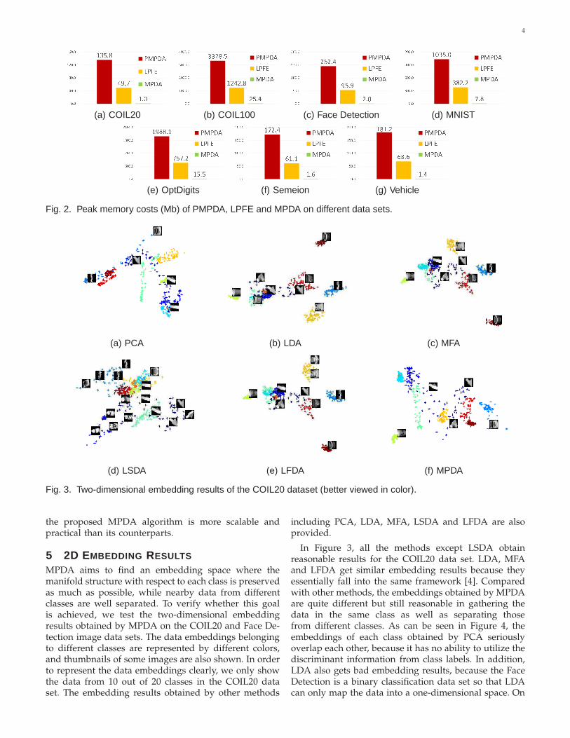
Apart from high computational costs, many tangentbased methods such as TSIMR [3] and PFE [2] are alsostorage consuming, which greatly hampers their appli-cations. In contrast, the proposed MPDA algorithm isfree from this limitation. In this section, we evaluate thestorage overheads of MPDA compared with its tangentspace based counterparts including PMPDA and LPFEon the COIL20, COIL100, Face Detection, MNIST, Opt-Digits, Semeion Handwritten and Vehicle data sets. Thenumber of the training data for each data set is the samewith the setting used in our paper. In order to obtainconsistent results, the neighborhood size for constructingthe within-class graph G is set to be k = 7, because thestorage costs of PMPDA and LPFE directly depend onk. Figure 2 shows the peak memory costs of PMPDA,LPFE and MPDA on different data sets. As can be seen,MPDA has the least storage overheads in all cases (about150 times and 60 times less than PMPDA and LPFE,respectively). In Figures 2(b) and 2(e), the peak memorycosts of PMPDA and LPFE are extremely high as thenumber of data becomes relatively large, whereas MPDAstill has very low memory costs. It should be noted thatthe above results are obtained under the condition ofk = 7. In practice, k may be larger, say k = 10 or k = 15.In this case, the storage overheads of PMPDA andLPFE grow quickly as k becomes large. Consequently,LPFE can barely work normally, and PMPDA is nolonger applicable because of out of memory. In contrast,MPDA still costs the same amount of memory becauseits storage overheads are independent of k. Therefore,

41 3 5 . 8 4 9 . 7 1 . 00 . 04 0 . 08 0 . 01 2 0 . 01 6 0 . 0 P M P D AL P F EM P D A(a) COIL20

3 3 2 8 . 5 1 2 4 2 . 8 2 5 . 40 . 01 0 0 0 . 02 0 0 0 . 03 0 0 0 . 04 0 0 0 . 0 P M P D AL P F EM P D A(b) COIL100

2 6 2 . 4 9 5 . 9 2 . 00 . 09 0 . 01 8 0 . 02 7 0 . 03 6 0 . 0 P M P D AL P F EM P D A(c) Face Detection

1 0 3 5 . 0 3 8 2 . 2 7 . 80 . 03 0 0 . 06 0 0 . 09 0 0 . 01 2 0 0 . 0 P M P D AL P F EM P D A(d) MNIST1 9 8 8 . 1 7 5 7 . 2 1 5 . 50 . 06 0 0 . 01 2 0 0 . 01 8 0 0 . 02 4 0 0 . 0 P M P D AL P F EM P D A

(e) OptDigits

1 7 2 . 4 6 1 . 1 1 . 60 . 05 0 . 01 0 0 . 01 5 0 . 02 0 0 . 0 P M P D AL P F EM P D A(f) Semeion

1 8 1 . 2 6 8 . 6 1 . 40 . 05 0 . 01 0 0 . 01 5 0 . 02 0 0 . 0 P M P D AL P F EM P D A(g) Vehicle

Fig. 2. Peak memory costs (Mb) of PMPDA, LPFE and MPDA on different data sets.

(a) PCA (b) LDA (c) MFA

(d) LSDA (e) LFDA (f) MPDA

Fig. 3. Two-dimensional embedding results of the COIL20 dataset (better viewed in color).

the proposed MPDA algorithm is more scalable andpractical than its counterparts.

5 2D EMBEDDING RESULTS

MPDA aims to find an embedding space where themanifold structure with respect to each class is preservedas much as possible, while nearby data from differentclasses are well separated. To verify whether this goalis achieved, we test the two-dimensional embeddingresults obtained by MPDA on the COIL20 and Face De-tection image data sets. The data embeddings belongingto different classes are represented by different colors,and thumbnails of some images are also shown. In orderto represent the data embeddings clearly, we only showthe data from 10 out of 20 classes in the COIL20 dataset. The embedding results obtained by other methods

including PCA, LDA, MFA, LSDA and LFDA are alsoprovided.

In Figure 3, all the methods except LSDA obtainreasonable results for the COIL20 data set. LDA, MFAand LFDA get similar embedding results because theyessentially fall into the same framework [4]. Comparedwith other methods, the embeddings obtained by MPDAare quite different but still reasonable in gathering thedata in the same class as well as separating thosefrom different classes. As can be seen in Figure 4, theembeddings of each class obtained by PCA seriouslyoverlap each other, because it has no ability to utilize thediscriminant information from class labels. In addition,LDA also gets bad embedding results, because the FaceDetection is a binary classification data set so that LDAcan only map the data into a one-dimensional space. On

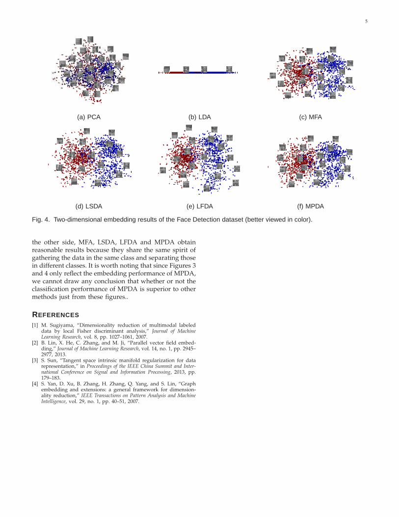
5

(a) PCA (b) LDA (c) MFA

(d) LSDA (e) LFDA (f) MPDA

Fig. 4. Two-dimensional embedding results of the Face Detection dataset (better viewed in color).

the other side, MFA, LSDA, LFDA and MPDA obtainreasonable results because they share the same spirit ofgathering the data in the same class and separating thosein different classes. It is worth noting that since Figures 3and 4 only reflect the embedding performance of MPDA,we cannot draw any conclusion that whether or not theclassification performance of MPDA is superior to othermethods just from these figures..

REFERENCES

[1] M. Sugiyama, “Dimensionality reduction of multimodal labeleddata by local Fisher discriminant analysis,” Journal of MachineLearning Research, vol. 8, pp. 1027–1061, 2007.

[2] B. Lin, X. He, C. Zhang, and M. Ji, “Parallel vector field embed-ding,” Journal of Machine Learning Research, vol. 14, no. 1, pp. 2945–2977, 2013.

[3] S. Sun, “Tangent space intrinsic manifold regularization for datarepresentation,” in Proceedings of the IEEE China Summit and Inter-national Conference on Signal and Information Processing, 2013, pp.179–183.

[4] S. Yan, D. Xu, B. Zhang, H. Zhang, Q. Yang, and S. Lin, “Graphembedding and extensions: a general framework for dimension-ality reduction,” IEEE Transactions on Pattern Analysis and MachineIntelligence, vol. 29, no. 1, pp. 40–51, 2007.

Documents

IEEE TRANSACTIONS ON CYBERNETICS 1 Manifold Partition