Liverpool Lectures on String TheoryThe Free Bosonic String

Summary NotesThomas Mohaupt

Semester 1, 2008/2009

Contents

1 The classical relativistic particle 21.1 Relativistic kinematics and dynamics . . . . . . . . . . . . . . . . 21.2 Action principle for the massive free particle: non-covariant version 31.3 Canonical momenta and Hamiltonian . . . . . . . . . . . . . . . . 41.4 Length, proper time and covariance on the world line . . . . . . . 51.5 Covariant action for the massive particle . . . . . . . . . . . . . . 61.6 Canonical momenta and Hamiltonian for the covariant action . . 91.7 Covariant action for massless and massive particles . . . . . . . . 9

2 The classical relativistic string 112.1 The Nambu-Goto action . . . . . . . . . . . . . . . . . . . . . . . 112.2 The Polyakov action . . . . . . . . . . . . . . . . . . . . . . . . . 14

2.2.1 Action, symmetries, equations of motion . . . . . . . . . . 142.2.2 Relation to two-dimension field theory . . . . . . . . . . . 152.2.3 Polyakov action in conformal gauge . . . . . . . . . . . . 162.2.4 Lightcone coordinates . . . . . . . . . . . . . . . . . . . . 172.2.5 Momentum and angular momentum of the string . . . . . 192.2.6 Fourier expansion . . . . . . . . . . . . . . . . . . . . . . . 21

3 The quantized relativistic string 233.1 Covariant quantisation and Fock space . . . . . . . . . . . . . . . 233.2 Implementation of constraints and normal ordering . . . . . . . . 263.3 Analysis of the physical states . . . . . . . . . . . . . . . . . . . . 28

3.3.1 The scalar ground state (tachyon) of the open string . . . 293.3.2 The massless vector state (photon) of the open string . . 303.3.3 Review of the Maxwell Lagrangian . . . . . . . . . . . . . 313.3.4 States of the closed string . . . . . . . . . . . . . . . . . . 343.3.5 The closed string B-field and axion . . . . . . . . . . . . . 353.3.6 The graviton and the dilaton . . . . . . . . . . . . . . . . 373.3.7 Review of the Pauli-Fierz Langrangian and of linearized

gravity . . . . . . . . . . . . . . . . . . . . . . . . . . . . . 40

A Literature 41

1

1 The classical relativistic particle

1.1 Relativistic kinematics and dynamics

D-dimensional Minkowski space(-time): M = MD = R

1,D−1.

Points = Events: x = (xµ) = (x0, xi) = (t, ~x),where µ = 0, . . . , D − 1, i = 1, . . . , D − 1 and we set c = 1.

Minkowski metric (‘mostly plus’):

η = (ηµν) =(−1 00 ID−1

). (1)

Scalar product (relativistic distance between events):

ηµνxµxν = xµxµ = −t2 + ~x2

< 0 for timelike distance,= 0 for lightlike distance,> 0 for spacelike distance.

(2)

World line of a particle:

x(t) = (xµ(t)) = (t, ~x(t)) . (3)

where t = time measured in some inertial frame.

Velocity :

~v =d~x

dt. (4)

Note:

~v · ~v{< 1(= c2) for massive particles (timelike worldline) ,= 1(= c2) for massless particles (lightlike worldline) . (5)

Proper time:

τ(t1, t2) =∫ t2

t1

dt√

1− ~v2 . (6)

To find τ(t), take upper limit to be variable:

τ(t1, t) =∫ t

t1

dt′√

1− ~v2 . (7)

Implies:dτ

dt=√

1− ~v2 =

√1− d~x

dt· d~xdt

. (8)

NB: this makes sense for massive particles, only, because we need ~v2 < 1. (Seebelow for massless particles).

2

Relativistic velocity:

xµ =dxµ

dτ=(dt

dτ,d~x

dt

dt

dτ

)=

(1, ~v)√1− ~v2

. (9)

Note that relativistic velocity is normalised:

xµxµ = −1 . (10)

Relativistic momentum (kinetic momentum):

pµ = mxµ = (p0, ~p) =(

m√1− ~v2

,m~v√1− ~v2

). (11)

NB: m is the mass (=total energy measured in the rest frame).For c = 1 note that E = p0 is the total energy, and:

pµpµ = −m2 = −E2 + ~p2 . (12)

In the rest frame we have E = m(= mc2).

Relativistic version of Newton’s second axiom:

d

dt~p =

d

dt

(m~v√1− ~v2

)= ~F , (13)

where ~F is the force acting on the particle.

NB: This is the correct relativistic version of Newton’s second axiom, but it isnot (yet) manifestly covariant.

1.2 Action principle for the massive free particle: non-covariant version

Action and Lagrangian:

S[~x] =∫dtL(~x(t), ~v(t)) . (14)

Action and Lagrangian for a free massive relativistic particle:

S = −m∫dt√

1− ~v2 = −mass times proper time . (15)

NB: we have set ~ = 1, action is dimensionless. The action of a particle isproportional to its proper time. The factor m is needed to make the actiondimensionless.

Action principle/Variational principle: the equations of motion are found byimposing that the action is stationary with respect to variations x→ x+ δx of

3

the path. Initial and final point of the path are kept fixed: δx(ti) = 0, wheret1 = time at initial position and t2 = time at final position.

Substitute variation of path into action and perform Taylor expansion:

S[~x+ δ~x,~v + δ~v] = S[~x,~v] + δS + · · · (16)

When performing the variation, we can use the chain rule:

δ√

1− ~v2 =∂

∂vi

√1− ~v2δvi (17)

(To prove this, you peform a Taylor expansion of the square root).~v, δ~v are not independent quanties:

δ~v = δd~x

dt=

d

dtδ~x . (18)

To find δS, we need to collect all terms proportional to δx. Derivatives actingon δx are removed through integration by parts. Result:

δS = −∫ t2

t1

(d

dt

mvi√1− ~v2

)δxidt+

mvi√1− ~v2

δxi∣∣∣∣t2t1

. (19)

Now use that the ends of the path are kept fixed (thus boundary terms vanish)and that the action principle requires δS = 0 for all choices of δx to obtain theequation of motion for a free massive particle:

d

dt

m~v√1− ~v2

=d

dt~p = 0 . (20)

1.3 Canonical momenta and Hamiltonian

Canonical momentum:πi :=

∂L

∂vi. (21)

For L = −m√

1− ~v2:πi = pi . (22)

Canonical momentum = kinetic momentum (not true in general. Example:charged particle in a magnetic field).

Hamiltonian:H(~x, ~π) = ~π · ~v − L(~x,~v(~x, ~π)) . (23)

Lagrangian→ Hamiltonian: go from variables (~x,~v) (coordinates and velocities)to new variables (~x, ~π) (coordinates and canonical momenta) by a Legendretransform:

H(~x, ~π) =∂L

∂~v· ~v − L(~x,~v(~x, ~π)) . (24)

4

For L = −m√

1− ~v2:

H = ~π · ~v − L = ~p · ~v − L =m√

1− ~v2= p0 = E . (25)

Thus: Hamiltonian = Total energy (not true in general. See below.)

Our treatment of the relativistic particle provokes the following questions:

• How can we include massless particles?

• How can we make Lorentz covariance manifest?

• How can we show that ‘the physics’ does not depend on how we parametrisethe world line?

We will answer these questions in reverse order.

1.4 Length, proper time and covariance on the world line

Mathematical description of a curve (for concreteness, a curve in Minkowskispace M):

C : R 3 σ −→ xµ(σ) ∈M . (26)

σ is an arbitrary curve parameter.

Tangent vectors of the curve:

x′µ :=

dxµ

dσ. (27)

Scalar products of tangent vectors, using Minkowski metric:

x′2 = ηµν

dxµ

dσ

dxν

dσ

> 0 for spacelike curves,= 0 for lightlike like curves (also called null curves),< 0 for timelike curves.

(28)Length of a spacelike curve:

L(σ1, σ2) =∫ σ2

σ1

√ηµν

dxµ

dσ

dxν

dσdσ . (29)

The length is independent of the parametrisation, i.e., it does not change if one’reparametrises’ the curve:

σ → σ(σ) , wheredσ

dσ6= 0 . (30)

Note that σ is an invertible, but otherwise arbitrary function of σ. Often oneimposes

dσ

dσ> 0 , (31)

5

which means that the orientation (direction) of the curve is preserved.

For timelike curves one can define analogously

τ(σ1, σ2) =∫ σ2

σ1

dσ

√−ηµν

dxµ

dσ

dxν

dσ(32)

and this is nothing but the proper time between the two events located at σ1

and σ2.To find τ (proper time) as a function of σ (arbitrary curve parameter), take

the upper limit to be variable:

τ(σ) =∫ σ

σ1

dσ′√−ηµν

dxµ

dσ′dxν

dσ′. (33)

Differentiate:dτ

dσ=

√−ηµν

dxµ

dσ

dxν

dσ. (34)

Compare tangent vector with relativistic velocity:

dxµ

dτ=dxµ

dσ

dσ

dτ=

dxµ

dσ√−ηµν dx

µ

dσdxν

dσ

. (35)

This implies (as required if τ is really proper time):

ηµνdxµ

dτ

dxν

dτ= −1 . (36)

Relativistic velocity = normalised tangent vector.

Use proper time τ instead of σ as curve parameter:∫ σ2

σ1

dσ

√−ηµν

dxµ

dσ

dxν

dσ=∫ τ2

τ1

dτ = τ2 − τ1 . (37)

This confirms that τ is indeed the proper time.

NB: Similarly, the expression for the length of a spacelike curve takes a simpleform when using the length itself as the curve parameter.

1.5 Covariant action for the massive particle

Use new, covariant expression for proper time to rewrite the action:

S[xµ, x′ µ] = −m∫dσ

√−ηµν

dxµ

dσ

dxν

dσ. (38)

This action does now depend on xµ (and the corresponding relativistic velocity),rather than on ~x (and the velocity). It is now covariant in the following sense:

6

• The action is invariant under reparametrisations σ → σ(σ) of the world-line. (Reparametrisations are by definition invertible, hence dσ

dσ 6= 0. )

• The action is manifestly invariant under Poincare transformations,

xµ → Λµνxν + aµ , (39)

where(Λµν) ∈ O(1, D − 1) and (aµ) ∈M (40)

are constant. (This is manifest, because the action is constructed out ofLorentz vectors).

Compute equations of motion through variation xµ → xµ + δxµ:

δS

δxµ= 0⇔ d

dσ

(m x′

µ√− x′ µ x′ µ

)= 0 . (41)

To get the physical interpretation, replace arbitrary curve parameter σ by propertime τ :

d

dτ

(mdxµ

dτ

)= mxµ = 0 . (42)

We claim that this is the same as (13) with ~F = ~0.More generally, the covariant version of (13) is

d

dτ

(mdxµ

dτ

)= fµ , (43)

where

(fµ) =(~v · ~F , ~F )√

1− ~v2(44)

is the relativistic force. To see that this is equivalent to (13), note

dp0

dt= ~v · d~p

dt(45)

(The change of energy per unit of time is related to the acting force ~F by~v · ~F . I.p., if the force and velocity are orthogonal, like for charged particle in ahomogenous magnetic field, the energy is conserved.)

Then (13) impliesdp0

dt= ~v · ~F . (46)

Multiplying by dτdt and using the chain rule we get the manifestly covariant ver-

sion (43) of (13). The additional equation for p0 is redundant, but is requiredfor having manifest covariance.

7

For a free massive particle the equation of motion is

mxµ = 0 . (47)

Solution = straight (world)line:

xµ(τ) = xµ(0) + xµ(0)τ . (48)

Actions with interaction

• If the force fµ comes from a potential, fµ = ∂µV (x), then the equation ofmotion (43) follows from the action

S = −m∫ √

−x2dτ −∫V (x(τ))dτ . (49)

For simplicity, we took the curve parameter to be proper time. In the sec-ond term, the potential V is evaluated along the worldline of the particle.

• If fµ is the Lorenz force acting on a particle with charge q, fµ = Fµν xν ,then the action is

S = −m∫ √

−x2dτ − q∫Aµdx

µ . (50)

In the second term, the (relativistic) vector potential Aµ is integratedalong the world line of the particle∫

Aµdxµ =

∫Aµ(x(τ))

dxµ

dτdτ . (51)

The resulting equation of motion is

d

dτ

(mdxµ

dτ

)= qFµν xν , (52)

where Fµν = ∂µAν − ∂νAµ is the field strength tensor. Equation (52) isthe manifestly covariant version of

d~p

dt= q

(~E + ~v × ~B

). (53)

• The coupling to gravity can be obtained by replacing the Minkowsk metricηµν by a general (pseudo-)Riemannian metric gµν(x):

S = −m∫dτ√−gµν(x)xµxν . (54)

The resulting equation of motion is the geodesic equation

xµ + Γµνρxν xρ = 0 . (55)

8

1.6 Canonical momenta and Hamiltonian for the covariantaction

Action and Lagrangian:

S =∫Ldσ = −m

∫dσ√− x′ 2 . (56)

Canonical momenta:

πµ =∂L

∂ x′ µ= m

x′µ√

− x′ 2= mxµ . (57)

Canonical momenta are dependent:

πµπµ = −m2 (58)

Going from a general curve parameter σ to proper time τ we see that

πµ = pµ (59)

and the constraint is recognised as the mass shell condition p2 = −m2.

Hamiltonian:H = πµxµ − L = 0 (60)

Hamiltonian 6= Total energy. Rather Hamiltonian = 0. Typical for covariantHamiltonians. Reason: canonical momenta not independent. The ’Hamilto-nia constraint’ H = 0 defines a subspace of the phase space. Solutions to theequations of motion live in this subspace. H = 0 does not mean that the dy-namics is trivial, it just reflects that the momenta are dependent. To stress thisone sometimes writes H ≈ 0 (read: H is weakly zero). One can also write:H = λ(p2 +m2), where λ is an arbitrary constant. In this form it is clear thatthe Hamiltonian is not identically zero (strongly zero, implying trivial physics),but that it vanishes whenever the particle satisfies the mass shell conditionp2 = −m2.

We still need to find a way to include massless particles.

1.7 Covariant action for massless and massive particles

Introduce invariant line element edσ, where e = e(σ) transforms under reparametri-sations such that edσ is invariant:

e(σ) = e(σ)dσdσdσ = dσ dσdσ

}⇒ edσ = edσ . (61)

Action:

S[x, e] =12

∫edσ

(1e2

(dxµ

dσ

)2

−m2

). (62)

9

We allow m2 ≥ 0. (In fact, we could allow m2 to become negative, m2 < 0.)

Symmetries of the action:

• S[x, e] is invariant under reparametrisations σ → σ.

• S[x, e] is invariant under Poincare transformations xµ → Λµνxν + aµ.

The action depends on the fields x = (xµ) and e. The corresponding equationsof motion are found by variations x→ x+ δx and → e+ δe, respectively.

Equations of motion:

d

dσ

(x′µ

e

)= 0 , (63)

x′2 + e2m2 = 0 . (64)

The equation of motion for e is algebraic. e is an auxiliary field, not a dynamicalfield. If m2 6= 0, we can solve for e:

e2 = − x′ 2

m2(65)

For massive particles we have m2 > 0 and x′2< 0, so that e2 is positive. We

take the positive root:

e =

√− x′ 2

m. (66)

Substituting the solution for e into (62) we recover the action (38) of a massiveparticle. However, the new action allows us to deal with massless particles aswell.

According to (64), e controlls the norm of the tangent vector, which can bechanged by reparametrisation. Instead of eliminating e by its equation of mo-tion, we can bring it to a prescribed ‘gauge’ (=parametrisation).

• For m2 > 0, impose the gauge

e =1m

(67)

The equations of motion become:

xµ = 0 (68)x2 = −1 (69)

Comment: in this gauge, σ becomes proper time τ .

• For m2 = 0, impose the gauge

e = 1 . (70)

10

The equations of motion become:

xµ = 0 , (71)x2 = 0 . (72)

Comment: for m2 = 0, (64) tells us that the worldline is lightlike, asexpected for a massless particle. In this case there is no proper time, butone can choose a so-called affine parametrisation. e = 1 (or any otherconstant value) corresponds to picking an affine parameter.

Note that in both cases the dynamical equation of motion xµ = 0 must besupplemented by a constraint,

φ ={x2 + 1x2

}= 0 (73)

to capture the full information.

2 The classical relativistic string

2.1 The Nambu-Goto action

Replace particle by one-dimensional string. Worldline becomes a surface, calledthe worldsheet Σ.

X : Σ 3 P −→ X(P ) ∈M . (74)

Coordinates on M are X = (Xµ), where µ = 0, 1, . . . , D − 1.Coordinates on Σ are σ = (σ0, σ1) = (σα). The worldsheet has one spacelikedirection (‘along the string’) and one timelike direction (‘point on the stringmoving forward in time’). Take σ0 to be time-like, σ1 to be space-like:

X2 ≤ 0 , (X ′)2 > 0 . (75)

We use the following notation:

X = (∂0Xµ) =

(∂Xµ

∂σ0

),

X ′ = (∂1Xµ) =

(∂Xµ

∂σ1

). (76)

Range of worldsheet coordinates:

• Spacelike coordinate:σ1 ∈ [0, π] . (77)

• Timelike coordinateσ0 ∈ (−∞,∞) , (78)

11

for propagation of a non-interacting string for infinite time, or

σ0 ∈ [σ0(1), σ

0(2)] . (79)

for propagation of a non-interacting string starting for a finite intervall oftime).

Nambu-Goto action ∼ area of world sheet:

SNG[X] = −TA(Σ) = −T∫

Σ

d2A (80)

T has dimension (length)−2 or energy/length = string tension (~ = c = 1).Invariant area element on Σ (induced from M):

d2A = d2σ√|det(gαβ)| , (81)

wheregαβ = ∂αX

µ∂βXνηµν (82)

is the induced metric (pull back). Note det(gαβ) < 0.Action is invariant under reparametrizations of Σ,

σα → σα(σ0, σ1) , where det(∂σα

∂σβ

)6= 0 . (83)

Action is also invariant under Poincare transformations of M.Action, more explicitly:

SNG =∫d2σL = −T

∫d2σ

√(XX ′)2 − X2(X ′)2 . (84)

L is the Lagrangian (density). We compute

Πµ = Pµ0 =∂L∂Xµ

= T(X ′)2Xµ − (XX ′)X ′µ√

(XX ′)2 − X2(X ′)2

,

Pµ1 =∂L∂X ′µ

= TX2X ′µ − (XX ′)Xµ√

(XX ′)2 − X2(X ′)2

. (85)

Πµ is the canonical momentum, Pµα are the momentum densities on Σ.The equations of motion are found by variations X → X + δX of the

worldsheet, where the initial and final configuration are kept fixed, δX(σ0 =σ0

(1), σ0(2)) = 0. Since the ends of the string are not fixed for other values of σ0,

variation yields a boundary term, which we need to require to vanish:∫dσ0

[∂L∂X ′µ

δXµ

]σ1=π

σ1=0

!= 0 . (86)

This boundary term must vanish ⇒ admissible boundary conditions.

12

1. Periodic boundary conditions:

X(σ1) = X(σ1 + π) (87)

Closed strings, the world sheet does not have (time-like) boundaries.

2. Neumann boundary conditions:

∂L∂X ′µ

∣∣∣∣σ1=0,π

= 0 (88)

(also called: free boundary conditions, natural boundary conditions).Open strings, ends can move freely. (The ends of an open string alwaysmove with the speed of line and thus their worldlines are light-like.)The momentum at the end of the string is conserved. (Pµ1 is the momen-tum density along the space-like direction of Σ, i.e., along the string at agiven ‘time’.)

3. Dirichlet boundary conditions:

Xi(σ1 = 0) = x0 , Xi(σ1 = π) = x1 . (89)

Open strings with ends kept fixed along the i-direction (spacelike).(Dirichlet boundary conditions in the time direction make only sense inimaginary time, in the Euclidean version of the theory, where they de-scribe instantons).

Consider Neumann boundary conditions along time and p spacelike con-ditions and Dirichlet boundary conditions along D − p directions. Thenthe ends of the string are fixed on p-dimensional spacelike surfaces, calledDirichlet p-branes. Momentum is not conserved at the ends of the stringin the Dirichlet directions (obvious, since translation invariance is broken)⇒ p-branes are dynamical objects. Interpretation: strings in a solitonicbackground ( 6= vacuum).

Equations of motion (with either choice of boundary condition):

∂0∂L∂Xµ

+ ∂1∂L∂X ′µ

= 0 (90)

or∂αP

αµ = 0 (91)

Canonical momenta are not independent. Two constraints:

ΠµX ′µ = 0

Π2 + T 2(X ′)2 = 0 (92)

Canonical Hamiltonian (density):

Hcan = XΠ− L = 0 . (93)

13

2.2 The Polyakov action

2.2.1 Action, symmetries, equations of motion

Intrinsic metric hαβ(σ) on the world-sheet Σ, with signature (−)(+).Polyakov action:

SP[X,h] = −T2

∫d2σ√hhαβ∂αX

µ∂βXνηµν , (94)

where h = − det(hαβ) = |det(hαβ)|.Local symmetries with respect to Σ:

1. Reparametrizations σ → σ(σ), which act by

Xµ(σ) = Xµ(σ) ,

hαβ(σ) =∂σγ

∂σα∂σδ

∂σβhγδ(σ) . (95)

2. Weyl transformations:

hαβ(σ)→ e2Λ(σ)hαβ(σ) . (96)

Remarks:

1. A Weyl transformation is not a diffeomorphism, but the multiplicationof the metric by a positive function. Mathematicians usually call this aconformal transformation, because it changes the metric but preserves theconformal structure of (Σ, hαβ).

2. The invariance under Weyl transformation is special for strings, it doesnot occure for particles, membranes and higher-dimensional p-branes.

3. Combining Weyl with reparametrization invariance, one has three localtransformations which can be used to gauge-fix the metric hαβ completely.Thus hαβ does not introduce new local degrees of freedom: it is an auxil-iary (‘dummy’) field.

Global symmetries with respect to M: Poincare transformations.

Equations of motion from variations X → X + δX and hαβ → hαβ + δhαβ .

1√h∂α

(√hhαβ∂βX

µ)

= 0 , (97)

∂αXµ∂βXµ −

12hαβh

γδ∂γXµ∂δXµ = 0 . (98)

Boundary conditions: as before.

14

The X-equation (97) is the covariant two-dimensional wave equation, alter-natively written as

�Xµ = 0⇔ ∇α∇αXµ = 0⇔ ∇α∂αXµ = 0 (99)

The h-equation (98) is algebraic and can be used to eliminate hαβ in terms ofthe induced metric gαβ = ∂αX

µ∂βXνηµν . It implies

det(gαβ) =14

det(hαβ)(hγδgγδ)2 . (100)

Substituting this into the Polyakov action one gets back the Nambu-Goto action.More generally one can show that SP ≥ SNG, where equality holds if gαβ andhαβ are related by a Weyl transformation (i.e., they are conformally equivalent).

2.2.2 Relation to two-dimension field theory

Alternative point of view: Σ is a two-dimensional ‘space-time’, populated by Dscalar fields X = (Xµ), which take values in MD. The Polyakov action has theform of a standard for a two-dimension scalar field theory. More precisely, itdefines a two-dimensional sigma-model with ‘target space’ M.

More generally: Mechanics of p-brane (p-dimensional extended object) =Field theory on a p+ 1 dimensional space-time (the worldvolume of the brane).

The energy-momentum tensor of the two-dimensional field theory is:

Tαβ := − 1T

1√h

δSPδhαβ

=12∂αX

µ∂βXµ −14hαβh

γδ∂γXµ∂δXµ (101)

(Defining Tαβ by the Noether procedure gives a tensor which might differ fromthis by a total derivative.)

The h-equation of motion in terms of Tαβ :

Tαβ = 0 . (102)

(Remember that the h-equation is a constraint.)

This equation can also be interpreted as the two-dimensional Einstein equa-tion, since the variation of two-dimensional Einstein-Hilbert action vanishesidentically. The Polyakov action describes a two-dimensional sigma model whichis coupled to two-dimensional gravity.

Tαβ is conserved:∇αTαβ = 0 (103)

15

To show this, one needs to use the equations of motion. The equation holdsonly ‘on shell’.

Tαβ is traceless:hαβTαβ = 0 (104)

This follows directly from the definition of Tαβ . It holds ‘off shell’, independentlyof whether the equations of motion are satisfied.

2.2.3 Polyakov action in conformal gauge

Three local symmetries, while the intrinsic metric hαβ has three independentcomponents ⇒ can bring hαβ to standard form (locally):

hαβ → ηαβ =(−1 00 1

). (105)

The condition hαβ!= ηαβ is called the conformal gauge. Strictly speaking,

the gauge condition should be imposed on the equations of motion, not on theaction. For the case at hand the result is correct nevertheless. Therefore, let usfollow the naive procedure and start from the Polyakov action in the conformalgauge.

The action:

SP = −T2

∫d2σηαβ∂αX

µ∂βXµ . (106)

Equations of motion for X (variation of gauge-fixed action gives correctgauge fixed equations of motion):

�Xµ = −(∂20 − ∂2

1)Xµ = 0 (107)

This is the two-dimensional wave equation, which is known to have the generalsolution:

Xµ(σ) = XµL(σ0 + σ1) +Xµ

R(σ0 − σ1) . (108)

Interpretation: decoupled left- and rightmoving waves.Boundary conditions:

Xµ(σ1 + π) = Xµ(σ) periodicX ′µ∣∣σ1=0,π

= 0 Neumann

Xµ

∣∣∣σ1=0,π

= 0 Dirichlet (109)

The equations coming from the h variation must now be added by hand:

Tαβ = 0 (110)

Note that the trace of Tαβ is

Trace(T ) = Tαα = ηαβTαβ = −T00 + T11 . (111)

16

The trace of Tαβ vanishes identically (off shell), and therefore Tαβ = 0 givesonly rise to two independent non-trivial constraints:

T01 = T10 =12XX ′ = 0

T00 = T11 =14

(X2 +X ′2) = 0 (112)

These equations are equivalent to the constraints derived from the Nambu-Gotoaction.

We have two-dimensional energy-momentum conservation (from the X equa-tion):

∂αTαβ = 0 (113)

and tracelessness (without equations of motion):

hαβTαβ = 0 . (114)

Note that energy-momentum conservation is non-trivial because Tαβ only van-ishes on-shell.

2.2.4 Lightcone coordinates

Equation (108) suggests to introduce lightcone coordinates (null coordinates):

σ± := σ0 ± σ1 . (115)

We write σa, where a = +,− for lightcone coordinates and σα, where α = 0, 1for standard coordinates.

The Jacobian of the coordinate transformation and its inverse:

(J aα ) =

D(σ+, σ−)D(σ0, σ1)

=(

1 11 −1

)(J αa ) =

D(σ0, σ1)D(σ+, σ−)

=12

(1 11 −1

)(116)

Converting lower indices:

va = J αa vα , vα = J a

α va . (117)

Example: the lightcone derivatives

∂± =12

(∂0 ± ∂1) (118)

Converting upper indices:

wa = wαJ aα , wα = waJ α

a . (119)

Example: the lightcone differentials

dσ± = dσ0 ± dσ2 . (120)

17

When converting tensors, act on each index. Example: lightcone metric

hab = J αa J β

a hαβ . (121)

Explicitly: metric in standard coordinates

(hαβ) =(−1 00 1

)= (hαβ) . (122)

Metric in lightcone coordinates

(hab) = −12

(0 11 0

), (hab) = −2

(0 11 0

). (123)

The lightcone coordinates of the (symmetric traceless) energy-momentum tensorare:

T++ =12

(T00 + T01) , T−− =12

(T00 − T01) , T+− = 0 = T−+ . (124)

Note that the trace, evaluated in lightcone coordinates, is:

Trace(T ) = ηabTab = 2η+−T+− = −4T+− . (125)

Thus ‘traceless’ ⇔ T+− = 0.Action in lightcone coordinates:

SP = −T2

∫d2σηαβ∂αX

µ∂βXµ

=T

2

∫d2σ = (X2 −X ′2) = 2T

∫d2σ∂+X

µ∂−Xµ . (126)

Equations of motion in lightcone coordinates:

�Xµ = −(∂20 − ∂2

1)Xµ = −4∂+∂−Xµ = 0

⇔ ∂+∂−Xµ = 0 . (127)

Then, it is obvious that the general solution takes the form:

Xµ(σ) = XµL(σ0 + σ1) +Xµ

R(σ0 − σ1) . (128)

The constraints in lightcone coordinates

T++ = 0 ⇔ ∂+Xµ∂+Xµ = 0⇔ X2

L = 0 ,

T−− = 0 ⇔ ∂−Xµ∂−Xµ = 0⇔ X2

R = 0 . (129)

We did not list T+− = 0 as a constraint, because it holds off shell. There aretwo non-trivial constraints, which are equivalent to the two constraints obtainedfor the Nambu-Goto action.

18

Energy-momentum conservation in lightcone coordintes:

∂−T++ = 0 T++ = T++(σ+)∂+T−− = 0 T−− = T−−(σ−) (130)

These equations are non-trivial, because T±± only vanish on shell.Using this, we see that every function f(σ+) defines a conserved chiral cur-

rent∂−(f(σ+)T++) = 0 (131)

and thus a conserved charge

Lf = T

∫ π

0

dσ1f(σ+)T++ . (132)

To show directly that Lf is conserved, ddσ0Lf = 0, you need to use the periodicity

properties of the fields in addition to current conservation. Similarly we obtainconserved quantities from T−− using a function f(σ−). For closed strings weget two different sets of conserved quantities. For open strings T++ and T−−are not independent, because they are related through the boundary conditons.Therefore one only gets one set of conserved charges.

The canonical momenta:

Πµ =∂LP∂Xµ

= TXµ (133)

The canonical Hamiltonian

Hcan =∫ π

0

dσ1(XΠ− LP

)=T

2

∫ π

0

dσ1(X2 +X ′2

)= T

∫ π

0

dσ1((∂+X)2 + (∂−X)2

)(134)

is the integrated version of the constraint T00 = T11 = 0.

NB: The conformal gauge does not provide a complete gauge fixing. Theaction is still invariant under residual gauge transformations. Namely, we cancombine conformal reparametrisations with a compensating Weyl transforma-tion (see below).

2.2.5 Momentum and angular momentum of the string

Polyakov action is invariant under global Poincare transformations of M :

Xµ → ΛµνXν + aµ (135)

Momentum is the quantity which is preserved when there is translation invari-ance (Noether theorem). Noether trick: promote the symmetry under consid-eration (here translations in M) to a local transformation: δXµ = δaµ(σ). The

19

action is no longer invariant, but it becomes invariant when aµ is constant.Therefore the variation of the action with respect to the local transformationmust take the form

δS =∫d2σ∂αa

µPαµ . (136)

Integration by parts gives

δS = −∫d2σaµ∂αP

αµ . (137)

If we impose that the equations of motion are satisfied, this must vanish for anyaµ. Hence the current Pαµ must be conserved on shell:

∂αPαµ = 0 . (138)

Interpretation Pαµ (µ fixed) is the conserved current on Σ associated with trans-lations in the µ-direction of M, in other words, the momentum density alongthe µ-direction. (From the point of view of the two-dimensional field theoryliving on Σ, translations in M are internal symmetries.)

While above we assumed the conformal gauge, the method works withoutgauge fixing.Explicitly:

Pαµ = −T√hhαβ∂βXµ

c.g.= −T∂αXµ , (139)

where we only went to the conformal gauge in the last step.To find the angular momentum density, do the same for Lorentz transfor-

mations in M. Result:Jαµν = XµP

αν −XνP

αµ (140)

While current conservation holds by construction, it can easily be checkedexplicitly, using the equations of motion: ∇αPαµ = 0, ∇αJαµν = 0.

Conserved charges are obtained by integration of the timelike component ofthe current along the spacelike direction of Σ:

Pµ =∫ π

0

dσ1P 0µ = T

∫ π

0

dσ1Xµ

Jµν =∫ π

0

dσ1J0µν = T

∫ π

0

dσ1(XµXν −XνXµ

)(141)

Again, these charges are conserved by construction, but one can also checkexplicitly ∂0Pµ = 0, ∂0Jµν = 0.

Summary: Pµ, Jµν are the total momentum and angular momentum of thestring, Pαµ , J

αµν the corresponding conserved densities on the world sheet.

20

2.2.6 Fourier expansion

For periodic boundary condition we write the general solution as a Fourier series:

Xµ(σ) = xµ +1πT

pµσ0 +i

2

√1πT

∑n 6=0

1nαµne

−2inσ− +i

2

√1πT

∑n 6=0

1nαµne

−2inσ+

(142)where xµ, pµ are real and αµn

? = αµ−n, αµn? = αµ−n.

NB: no linear term in σ1, because of boundary condition. Splitting of zeromode between left and rightmoving part arbitrary.

pµ is the total momentum:

Pµ = T

∫ π

0

dσ1Xµ = pµ . (143)

The center of mass of the string moves along a straight line, like a relativisticparticle:

xµcms =1π

∫ π

0

dσ1Xµ(σ) = xµ + pµσ0 = xµ(0) +dxµ

dτ(0)τ (144)

Thus: string = relativistic particle plus left- and rightmoving harmonic oscilla-tions.

Formulae suggest to use ‘string units’:

T =1π. (145)

(On top of c = ~ = 1).Fourier components of

T±± =12

(∂±X)2 (146)

at σ0 = 0:

Lm := T

∫ π

0

dσ1 e−2imσ1T−− =

πT

2

∞∑n=−∞

αm−n · αn ,

Lm := T

∫ π

0

dσ1 e2imσ1T++ =

πT

2

∞∑n=−∞

αm−n · αn , (147)

whereα0 = α0 =

1√4πT

pπT=1=

12p . (148)

The constraints T±± = 0 imply

Lm = Lm = 0 . (149)

21

The Lm are conserved, take f ∼ e2imσ1in (132). If the constraint hold at σ0 = 0

they hold for all times σ0. The constraints are conserved under time evolution.Canonical Hamiltonian:

H =∫ π

0

dσ1(XΠ− L

)=T

2

∫ π

0

(X2 + (X ′)2)2 = L0 + L0 (150)

(The world sheet Hamiltonian L0 + L0 generates translations of σ0, see below.)The ‘Hamiltonian constraint’ H = 0 allows us to express the mass of a state

in terms of its Fourier modes:

H = L0 + L0 =πT

2

∞∑n=−∞

(α−n · αn + α−n · αn)

=p2

4+ πT (N + N) = 0 (151)

where we defined the total occupation numbers

N =∞∑n=1

α−n · αn , N =∞∑n=1

α−n · αn .

This implies the ‘mass shell condition’:

M2 = −p2 = 4πT (N + N) .

Since L0 = L0 we have the additional constraint

N = N ,

which is called level matching, because it implies that left- and rightmovingmodes contribute equally to the mass.

Open string with Neumann boundary conditions:

Xµ(σ) = xµ + pµσ0 +i√πT

∑n6=0

1nαµne

−inσ0cos(nσ1) . (152)

This can still be decomposed into left and rightmvoing parts X = XL(σ+) +XR(σ−):

XµL/R(σ±) =

12xµ +

1πT

pµL/Rσ± +

i

2√πT

∑n 6=0

1nαµn (L/R)e

−inσ± , (153)

but the boundary conditions X ′µ(σ1 = 0, π) = 0 imply

pL = pR =12p , αn(L) = αn(R) . (154)

We see that due to the boundary conditions left and rightmoving waves arereflected at the boundaries and combine into standing waves. There are onlyhalf as many independent oscillations as for closed strings.

22

Combining the boundary conditions with the constraints we see that (Xµ)2(σ1 =0, π) = 0 ⇒ The ends of the string move with the speed of light.

Since XL and XR are related by σ1 → −σ1 (world sheet parity), we cancombine them into one single periodic field with doubled period, σ1 ∈ [−π, π].

Fourier decomposition gives one set of modes,

Lm = 2T∫ π

0

dσ1(eimσ

1T++ + e−imσ

1T−−

)=T

4

∫ π

−πeimσ

1(X +X ′

)2

=12πT∑n

αm−nαn (155)

where we defined α0 = p. The canonical Hamiltonian is H = L0.The Lm define the constraints: Lm = 0 and these constraints are conserved

in time. (Note that we only get ‘half as many’ constraints as for the bosonicstring, due to the boundary conditions.) The Hamiltonian constraint H = L0 =0 is the mass shell condition:

M2 = −p2 = 2πTN .

Dirichlet boundary conditions: linear term in σ1, but no linear time in σ0.For the osciallators, cos is replaced by sin. Thus X = 0 at the ends (ends don’tmove), but X ′ 6= 0 at the ends, corresponding to exchange of momentum witha D-brane.

3 The quantized relativistic string

3.1 Covariant quantisation and Fock space

We set πT = 0 in the following (on top of ~ = 1 = c).Remember quantization of non-relativistic particle:

[xi, pj ] = iδij ,

where i = 1, 2, 3. Here πi = pi is the canonical (=kinetic) momentum.Relativistic particle:

[xµ, pν ] = iηµν .

The canonical (=kinetic) momentum is now constrained by the mass shell con-dition p2 +m2 = 0.

Free scalar field:

[φ(x), φ(y)]x0=y0 = iδ(3)(~x− ~y)

Note that the commutator is evaluated at equal times x0 = y0. The canonicalmomentum of a free scalar field φ(x) is Π(y) = ∂L

∂(∂0φ(x)) = ∂0φ(x) = φ(x).Free relativistic string:

[Xµ(σ0, σ1),Πν(σ′0, σ′1)]σ0=σ′0 = iηµνδ(σ1 − σ′1) .

23

Here δ(σ) = δ(σ + π) is the periodic δ-function, which has the Fourier series

δ(σ) =1π

∞∑k=−∞

e−2πikσ/π =1π

∞∑k=−∞

e−2ikσ .

We are working in the conformal gauge where �Xµ = 0, resulting in the Fourierexpansions (142), (152), depending on our choice of boundary conditions. Inthe conformal gauge, the canonical momentum is

Πµ =∂L

∂(∂0Xµ)= TXµ =

1πXµ .

Using the Fourier expansion, we can derive the commutation relations for themodes

[xµ, pν ] = iηµν , [αµm, ανn] = mδm+n,0η

µν , [αµm, ανn] = mδm+n,0η

µν . (156)

Hermiticity of Xµ implies:

(xµ)+ = xµ , (pµ)+ = pµ , (αµm)+ = αµ−m .

We get the commutation relations of a relativistic particle plus those of aninfinite number of harmonic oscillators, (with frequencies ωm = m > 0, see later)corresponding to the excitations of the string. To obtain standard creation andannihilation operators, set

aµm =αµ√m

for m > 0 ,

(aµm)+ =αµ√−m

for m < 0 , (157)

to obtain [aµm, (aνn)+] = ηµνδm,n, which generalises [a, a+] = 1.

As a first step to constructing the Hilbert space of states we construct arepresentation space of the operators x, p, α, which we call the Fock space F .This space is different from the physical Hilbert space H, because we still haveto implement the constraints Lm ≈ 0 (and, for closed strings Lm ≈ 0).

The ground state |0〉 of F is defined by two conditions: it is translationinvariant (=does not carry momentum) and it is annihilated by all annihilatinoperators αµm, m > 0:

pµ|0〉 = 0 , αµm|0〉 = 0 for m > 0 .

Momentum eigenstates are defined by the property

pµ|k〉 = kµ|k〉 ,

where pµ is the momentum operator and k = (kµ) its eigenvalue. Momentumeigenstates can be constructed out of the ground state using the operator xµ:

|k〉 = eikx|0〉 ,

24

where kx = kµxµ. Exciteted string states are generated by applying creation

operators. I.p.αµ−m|0〉

is a state with excitation number Nµm = 1 in the m-th mode along the µ-

direction. A general excited state is a linear combination of states of the form

αµ1−m1

αµ2−m2· · · |0〉 ,

which have definit excitation numbers {Nµm}. A basis for F is obtained by

taking linear combinations of states of the form

αµ1−m1

αµ2−m2· · · |k〉 ,

which carry momentum k = (kµ) and excitation numbers {Nµm|µ = 0, . . . , D −

1, m > 0}.The Fock space F carries a natural scalar product. Let us first define it in

the oscillator sector. Decompose the ground state into an oscillator groundstate|0〉osc and a momentum groundstate |0〉mom:

|0〉 = |0〉osc ⊗ |0〉mom .

The scalar product in the oscillator sector is fixed by the properties of thecreation and annihilation operators αµm, once we have normalised the groundstate:

osc〈0|0〉osc = 1 .

For illustration, we compute:(αµ−m|0〉osc, α

ν−n|0〉

)= osc〈0|αµmαν−n|0〉osc = osc〈0|[αµm, αν−n]|0〉osc = mηµνδm+n,0 .

This scalar product is manifestly Lorentz covariant, but indefinit, i.e. there arestates of negative norm. This shows that F is not a Hilbert space. This is nota problem, as long as the physical space of states is positiv definit.

The scalar product between momentum eigenstates is

〈k|k′〉 = δD(k − k′) .

This is not defined if k = k′. Momentum eigenstates |k〉, including the momen-tum ground state 0〉mom, are not normalisable. Normalisable states are obtainedby forming momentum space wave packets

|φ〉 =∫dDkφ(k)|k〉

where φ(k) (the momentum space wave function) is square integrable:

〈φ|φ〉 =∫dDkφ(k)φ(k) <∞ .

25

3.2 Implementation of constraints and normal ordering

Having constructed the Fock space F , we still need to impose the constraintsLm ≈ 0 ≈ Lm. Naively we expect that the resulting space Fphys of physicalstates is positiv definit. As we will see in due course, the situation is a bit morecomplicated. For now we need to decide how to implement the constraints.We decide to require that the matrix elements of the operators Lm, Lm vanishbetween physical states vanish. Naively, this amounts to saying: a state |φ〉 isa physical state, |φ〉 ∈ Fphys, if

〈φ|Lm|φ〉 = 0 ,

and, for closed strings, in addition

〈φ|Lm|φ〉 = 0 ,

for all m. But as it stands this is ambiguous, because the Lm are quadratic inthe α’s, which do not commute any more in the quantum theory. Thus we havean ordering ambiguity in the quantum theory, which we need to investigate.

One standard ordering prescription is normal ordering, which requires to putall annihilation operators to the right of the creation operators:

: αµmανn :=

αµmανn if m < 0, n > 0

ανnαµm if m > 0, n < 0

any ordering if else.

From the commutation relations (156) we see that normal ordering only has anon-trivial effect if m = −n and µ = ν, because creation and annihilation oper-ators corresponding to different excitations levels or different directions comm-mute.

Compute the normally ordered version of L0:

LNO0 =

12

∞∑n=−∞

: α−n · αn :

=12

−1∑n=−∞

: α−n · αn : +12α0 · α0 +

12

∞∑1

: α−n · αn :

=18p2 +N , (158)

where we used that 12α0 · α0 = 1

8p2 for closed strings and defined the number

operator

N =∞∑n=1

α−n · αn .

Now compare this to what we might call the classically ordered version of L0:

LCO0 =

12

∞∑n=−∞

α−n · αn

26

=12

−1∑n=−∞

α−n · αn +12α0 · α0 +

12

∞∑1

α−n · αn

=18p2 +

12

∞∑1

(αn · α−n + α−n · αn) (159)

Both version of L0 differ by an infinite constant:

LCO0 − LNO

0 =D

2

∞∑n=1

n .

Going from the classically ordered to the normally ordered L0 amounts to sub-tracting an infinite constant. We will take the quantum version of L0 to be thenormally ordered one, L0 = LNO

0 . This is prescription usually adopted in quan-tum field theory. But is this the correct choice? The problem is not that theconstant which we subtract is infinite (we have the freedom to define any unde-fined object as we like), but that there is a finite ambiguity in this procedure.In other words: why don’t we take LNO0 + a, where a is some finite constant?(Equivalently, why can’t we adopt a slightly different ordering prescription forfinitely many term, which shifts L0 by a finite constant?)

There are two ways to procede from here. The first is to accept that theordering of L0 is ambiguous, and to formulate the constraint in the form

〈φ|L0 − a|φ〉 = 0 , 〈φ|L0 − a|φ〉 = 0 ,

where L0, L0 are normally ordered and a, a are finite constants which parametrizethe ambiguity. It then turns out that in order to have a postive definit spaceof states, one must choose a = a = 1, i.e., the ambiguity is completely fixed byphysical requirements.

The other way, which gives the same result, is to find a physcial procedure forcomputing a. The basic insight is that the infinite constant which is subtractedcorresponds to the ground state energies of infinitely many harmonic oscillators.To show this, remember that L0 = 1

8p2 +N (closed string). The commutation

relation of N with a creation operator is

[N,αµ−m] = mαµ−m .

ThusNαµ−m|0〉 = mαµ−m|0〉

andNαµ1−m1

αµ2−m2· · · |0〉 = (m1 +m2 + · · ·)αµ1

−m1αµ2−m2· · · |0〉

where the eigenvalue m1 +m2 + · · · of N is the total excitation number. ThusN counts excitations (weighted with their level), hence the name. Now rewriteN in terms of canonically normalised creation and annihilation operators (157):

N =∞∑n=1

α−n · αn =∞∑n=1

na+n · an

27

Comparing this to the Hamilton operator of a harmonic oscillator of frequencyωn = n > 0 (~ = 1),

Hn = n(a+n an +

12

)

we see that N differens from∑∞n=1Hn by the (divergent) sum over the ground

state energies n2 . We will discuss later how this sum can be regularized and

computed.1

For the time being we parametrise the normal ordering ambiguity by a, a. Itis straightforward to show that the Lm, m 6= 0 do not suffer from a normal or-dering ambiguity. The resulting definition of physical states is: |φ〉 is a physicalstate, |φ〉 ∈ Fphys, if

〈φ|Lm|φ〉 = 0 , 〈φ|Lm|φ〉 = 0 for m 6= 0 , and〈φ|L0 − a|φ〉 = 0 , 〈φ|Lm − a|φ〉 = 0 . (160)

3.3 Analysis of the physical states

We will now start to analyse Fphys. The hermiticity properties L+m = L−m can

be used to write the constraints in the form

Lm|φ〉 = 0 , Lm|φ〉 = 0 for m > 0 ,(L0 − a)|φ〉 = 0 , (Lm − a)|φ〉 = 0 . (161)

We start with the L0-constraint.

(L0 − a)|φ〉 = 0

⇒ (18p2 +N)|φ〉 = a|φ〉

⇒ 18k2 +N = a , (162)

where k is the momentum and N denotes, in the last line, the eigenvalue of theoperator N . In the future, we will use N to denote both the operator and itseigenvalue. The meaning should be clear from the context.

Since k2 = −M2, where M is the mass, we see that this constraint expressesthe mass in terms of the total leftmoving excitation number:

18M2 = N − a .

In the rightmoving sector we find

18M2 = N − a .

1In QFT non-trivial effects of the ground state energy can usually be ignored, because one(i) does not couple to gravity and (ii) works in infinite volume. In finite volume, the vacuumenergy depends explicitly on the volume. This is a measurable effect, the Casimir effect. Sincestrings have finite size, the Casimir effect cannot be ignored, and its computation leads toa = 1. See later.

28

Both conditions can be recombined into the mass shell condition

14M2 = N + N − a− a

which expresses the mass in terms of left- and rightmoving excitation numbers,and the level matching condition

N − a = N − a ,

which states the left- and rightmoving degrees of freedom contribute symmetri-cally to the mass.

This formula is given in string units, πT = 1. The string tension can easilybe re-installed by dimensional analysis. Traditionally, the mass formula is thenexpressed in terms of the Regge slope

α′ =1

2πT

rather than in terms of the string tension T :

α′M2 = 2(N + N − a− a) .

The Regge slope has dimension Length2.√α′ can be regarded as the funda-

mental string length. String units correspond to setting α′ = 12 .

For open strings we have L0 = 12p

2+N , and the resulting mass shell conditionis

α′M2 = N − a .

Let us now have a look at the lowest mass states. When listing these weanticipate that a = a = 1. Start with the open string:

N α′M2 State Spin0 −1 |k〉 Scalar1 0 αµ−1|k〉 Vector2 1 αµ−2|k〉 Vector

αµ−1αν−1|k〉 Symmetric Tensor

We still have to impose the further constraints Lm|φ〉 = 0 for m > 0. For|φ〉 = |k〉 it is easy to see that the other conditions are satisfied automatically.This state is physical, and having minimal mass-squared it is the physical groundstate of the relativistic string.

3.3.1 The scalar ground state (tachyon) of the open string

Thus the physical ground state of string is a scalar with negative mass-squared,a tachyon. Note that this state is a tachyon for any positive a. Taken as classicalparticles, tachyons propagate faster than the speed of light and are believed to beunphysical. The interpretation quantum field theory is more subtle. The mass-squared of a particle is given by the second derivative of the scalar potential

29

at its minimum. If the second derivative of the potential is negative ratherthan positive, this means that one is looking at a local maximum and not at aminimum of the potential. This means that the true vacuum is elsewhere, at afinite value of the expectation value of the ‘tachyon’ (tachyon condensation). Inthe standard model, the Higgs field has negative mass squared when expandingthe around the local maximum of the Higgs potential. However, the physicalHiggs particle is found by expanding the potential around the minimum, andit has a positive mass-squared, given by the curvature of the potential at itsminimum. Something similar happens for the open string. The true vacuum isbelieved to be the ground state of the closed string, i.e., the true vacuum doesnot have open string excitations.

While this is interesting, for us the relativistic string, open or closed, is onlya toy model anyhow, because, as we will see, it does not contain fermions in itsspectrum. The physically interesting string theories are supersymmetric stringtheories, where the ground state is massless rather than tachyonic. Thereforewe will regard the tachyon ground state as an unphysical feature of a toy model.

3.3.2 The massless vector state (photon) of the open string

The first excited state is a massless vector, hence potentially a photon. Notethat the first excited state is massless if and only if a = 1. For generic values ofa there would be no massless states at all. This indicates that the case a = 1 isspecial (though it does not prove that this is the correct value).

In this case the L1-constraint is non-trivial. Let us evaluate the constraintfor a general linear combination |φ〉 = ζµα

µ−1|k〉 of level-one states:2

L1|φ〉 = 0⇒ L1ζµα

µ−1|k〉 = 0

⇒ αν0ζν [α1,ν , αµ−1]|k〉 = 0

⇒ kµζµ|0〉 = 0 . (163)

Thus physical level-one states satisfy

k2 = 0 , kµζµ = 0 .

This tells us that the momentum is lightlike, corresponding to a massless par-ticle, and orthogonal (in Minkowski metric) to the vector ζ, which thereforeshould be interpreted as the polarisation vector.

Since one can show that Lmζµαµ−1|k〉 = 0 holds automatically for m > 1, all

these states are physical. Can we interprete these states as the components ofa photon? In D dimensions, a photon has D − 2 independent components dueto gauge invariance. The condition k · ζ = 0 reduces the number of independentpolarisations from D to D − 1. We have to show that there are actually onlyD − 2 independent components, and we would like to see the underlying gaugeinvariance.

2Here and in the following we write |k〉 instead of |0〉osc ⊗ |k〉 for simplicity.

30

To this end, consider states of the form

|ψ〉 = λkµαµ−1|k〉

where λ is a (real) constant.The scalar product of such a state with itself is zero:

〈ψ|ψ〉 = λ2kµkν〈k|[αµ1 , αν−1]|k〉 = λ2k2〈k|k〉 = 0

because k2 = 0.3 The state |ψ〉 = λkµαµ−1|k〉 is different from zero, |ψ〉 6= 0, yet

orthogonal to itself 〈ψ|ψ〉 = 0: it is a so-called null state. The existence of nullstates shows that Fphys cannot be postive definit and therefore that it is notthe physical Hilbert state. (More in due course).

One can also show that |ψ〉 is orthogonal to any state with excitation leveldifferent from 1. Moreover, it is orthogonal to any physical state with excitationlevel 1:

〈k′|αµ1 ζµkναν−1|k〉 = ζ · k〈k′|k〉 = 0 ,

because either k 6= k′ implying 〈k|k′〉 = 0 or k = k′, implying ζ · k = 0.This shows that |ψ〉 is a ‘spurious state’, because it drops out of any scalar

product between physical states. In other words

(ζµ + λkµ)αµ−1|k〉

represents the same physical state for any value of λ. The freedom of changingthe value of λ is a gauge degree of freedom. The component of ζ parallel to themomentum does not contribute to any physical quantity, and thus the numberof independent physical polarisations is reduced to D − 2, as expected for aD-dimensional photon.

3.3.3 Review of the Maxwell Lagrangian

For illustration, we review how the conditions k2 = 0 and k ·ζ = 0 can be derivedfrom electrodynamics. We start from the D-dimensional Maxwell action

S[A] =∫dDx

(−1

4FµνF

µν

),

whereFµν = ∂µAν − ∂νAµ .

By variation of Aµ we obtain one half of the Maxwell equations

∂µFµν = 0 .

In the presence of charge matter, the action becomes

S[A, j] =∫dDx

(−1

4FµνF

µν − jµAµ),

3Since 〈k|k〉 is not well defined, we should actually consider wave packets. But this is onlya technical complication, which does not change the result.

31

where jµ is the electromagnetic current. The resulting Maxwell equations are

∂µFµν = jν .

The second half of the Maxwell equations do not follow from the variation of theaction. They are identities (called Bianchi identities), which are the integrabilityconditions guaranteeing that the field strength has a vector potential:

∂[νFρσ] = 0⇔ Fµν = ∂µAν − ∂νAµ (locally) .

The field strength and the action are invariant under gauge transformations

Aµ → Aµ + ∂µχ⇒ Fµν → Fµν ,

where χ is an arbitrary function. Note that the coupling to a current jµ is onlyconsistent if the current is conserved, ∂µjµ = 0.

Let us restrict to free Maxwell theory, jµ = 0, and compare the propertiesof the photon field Aµ to those of the massless vector state of the open string.Writing out the equation of motion:

∂µFµν = �Aµ − ∂µ∂νAν = 0 .

We can partially fix the gauge symmetry by imposing the Lorenz gauge andobtain

�Aµ = 0 , if ∂νAν = 0 .

There is still a residual gauge symmetry because we can make gauge transfor-mations where the function χ satisfies �χ = 0, because

∂νAν → ∂ν(Aν + ∂νχ) = ∂νAν + �χ .

This implies that, in the Lorenz gauge, Aµ and Aµ+∂µχ with �χ = 0 representthe same physical state. The number of independent physical components ofAµ is D − 2.

Consider now a plane wave with momentum k and polarisation vector ζ:

Aµ = ζµeikx .

The general solution can be written a superposition (Fourier integral) of suchplane waves. This allows us to translate the equations of motion, the Lorenzgauge, and the residual gauge symmetry into momentum space:

�Aµ = 0 ⇔ kµkµ = 0∂µAµ = 0 ⇔ ζµkµ = 0

Aµ ' Aµ + ∂µχ ⇔ ζµ ' ζµ + λkµ (164)

We can be more explicit about the unphysical, physical and spurious parts ofAµ, by making an explicit choice for the momentum vector:

k = (k0, 0, . . . , 0, k0)

32

This corresponds to a massless particle (equivalently, a plane wave) propagationparallel to the (D − 1)-axis (for D = 4, the 3-axis or z-axis). The polarisationvector must satisfy:

k · ζ = 0⇒ −k0ζ0 + k0ζD − 1 = 0→ ζ0 = ζD−1 . (165)

Thus physical polarisation vectors have the form

ζ = (ζ0, ζ1, . . . , ζD−2, ζD−1) .

Introduce the following basis for polarisation vectors:

k = (k0, 0, . . . , 0, k0) ,

k =1

2(k0)2(−k0, 0, . . . , 0, k0) ,

ei = (0, . . . , 1, . . . , 0) , i = 1, . . . , D − 2 (166)

This is an orthonormal basis which consists of two linearly independent lightlikevectors spanning the light cone and D − 2 spacelike vectors which spann thedirections transverse to the light cone:

k · k = 0 , k · k = 1 , k · k = 0 ,ei · ej = δij , k · ei = 0 , k · ei = 0 . (167)

In this basis physical polarisation vectors have the form:

ζ = ζiei + αk ,

i.e. the unphysical direction in polarisation space is the one parallel to k (whichis the only basis vector with a nonvanishing scalar product with k).

However, the part of ζ which is parallel to k is spurious: it has zero norm andis orthogonal to any physical polarisation vector. The D− 2 physical degrees offreedom reside in the transverse part

ζtransv = ζiei = (0, ζ1, ζ2, . . . , ζD−2, 0)

We call this the transverse part, because the spatial part

~ζ = (ζ1, ζ2, . . . , ζD−2, 0)

is orthogonal to the spatial momentum

~k = (0, . . . , 0, k0) .

In D = 4, this is the well-known fact that a photon has two physical polarisa-tions, which are transverse to the momentum.

Group theoretical interpretation. In (165) we have made an explicit choicefor the momentum vector, which corresponds to the choice of a Lorentz frame.

33

This choice is not unique, we can still make Lorentz transformations which arespatial rotations around the axis spanned by k. The corresponding subgroup

SO(D − 2) ⊂ SO(1, D − 1)

is known as the little group. A central result in the representation theory of thePoincare group states that massless representations (those where pµpµ = −m2 =0) are classified by representations of the little group. The physical componentsof ζµα

µ−1|0〉 and of Aµ = ζµe

ikx transform in the vector representation [D − 2]of the little group SO(D − 2). This is what characterises them mathematicallyas a massless vector, or ‘photon’.

The case D = 4 is special, because the group SO(2) is abelian, which impliesthat its irreducible representations are one-dimensional. In D = 4 the transversepolarisation vector ζtransv = (ζ1, ζ2) transforms as follows:(

ζ1

ζ2

)→(

cosϕ − sinϕsinϕ cosϕ

)(ζ1

ζ2

).

To see the decomposition into two one-dimensional representations we take com-plex linear combinations

ζ± = ζ1 ± iζ2 .

This corresponds to going from a basis of transverse polarisations to a basis ofcircular polarisations. Now(

ζ+

ζ−

)→(eiϕ 00 e−iϕ

)(ζ+

ζ−

),

These states have helicity h = ±1. Mathematically, we have used the groupisomorphism SO(2) ' U(1).

In conclusion, the massless vector state of the open string has preciselythe kinetic properties which characterise a photon (=a massless vector bosonwith a gauge invariance). Therefore the Maxwell action provides a space-timedescription of the massless vector state of the free string: it is the effective actionof this state.

3.3.4 States of the closed string

Physical closed strings satisfy the mass shell and level matching conditions

α′M2 = 2(N + N − a− a)N = N (168)

plusLm|φ〉 = 0 = Lm|φ〉 for m > 0 . (169)

34

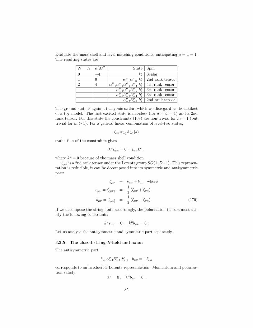
Evaluate the mass shell and level matching conditions, anticipating a = a = 1.The resulting states are

N = N α′M2 State Spin0 −4 |k〉 Scalar1 0 αµ−1α

ν−n|k〉 2nd rank tensor

2 4 αµ−1αν−1α

ρ−1α

σ−1|k〉 4th rank tensor

αµ−1αν−1α

ρ−2|k〉 3rd rank tensor

αµ−2αρ−1α

σ−1|k〉 3rd rank tensor

αµ−2αρ−2|k〉 2nd rank tensor

The ground state is again a tachyonic scalar, which we disregard as the artifactof a toy model. The first excited state is massless (for a = a = 1) and a 2ndrank tensor. For this state the constraints (169) are non-trivial for m = 1 (buttrivial for m > 1). For a general linear combination of level-two states,

ζµναµ−1α

ν−1|k〉

evaluation of the constraints gives

kµζµν = 0 = ζµνkν ,

where k2 = 0 because of the mass shell condition.ζµν is a 2nd rank tensor under the Lorentz group SO(1, D−1). This represen-

tation is reducible, it can be decomposed into its symmetric and antisymmetricpart:

ζµν = sµν + bµν where

sµν = ζ(µν) =12

(ζµν + ζνµ)

bµν = ζ[µν] =12

(ζµν − ζνµ) (170)

If we decompose the string state accordingly, the polarisation tensors must sat-isfy the following constraints:

kµsµν = 0 , kµbµν = 0 .

Let us analyse the antisymmetric and symmetric part separately.

3.3.5 The closed string B-field and axion

The antisymmetric part

bµναµ−1α

ν−1|k〉 , bµν = −bνµ

corresponds to an irreducible Lorentz representation. Momentum and polarisa-tion satisfy:

k2 = 0 , kµbµν = 0 .

35

One can show that physical states with

bµν = kµaν − kνaµ , where kµaµ = 0 ,

are spurious, i.e. they have zero norm and are orthogonal to all physical states.Thus we have identified a gauge symmetry

bµν → bµν + kµaν − kνaµ , where kµaµ = 0 .

This state is a massless, 2nd rank antisymmetric tensor and has a gauge sym-metry similar to the one of a photon. For a free field, the action is

S[B] =∫dDx

(− 1

2 · 3!HµνρH

µνρ

),

where

Hµνρ =33!

(∂µBνρ − ∂µBρν + ∂νBρµ − ∂νBµρ + ∂ρBµν − ∂ρBνµ)

= ∂µBνρ + ∂νBρµ + ∂ρBµν (171)

is the field strength (completely antisymmetric 3rd rank tensor) and Bµν (anti-symmetric 2nd rank tensor) is the gauge field (gauge potential). The equationof motion is

∂µHµνρ = 0 ,

and the Bianchi identity corresponding to the existence of a gauge potential is

∂[µHνρσ] = 0⇔ Hµνρ = ∂µBνρ + · · ·

The field strength Hµνρ and, hence, the action is invariant under gauge trans-formations

Bµν → Bµν + ∂µΛν − ∂νΛµ ,

where the gauge parameter is now a vector field Λµ (and has its own gaugeinvariance Λµ → Λµ + ∂µχ in turn). Writing out the equation of motion gives:

∂µ (∂µBνρ + ∂νBρµ + ∂ρBµν) = 0

This becomes the wave equation when we impose the analogon of the Lorenzgauge:

�Bµν = 0 , if ∂µBµν = 0 and �Λµ = 0 , ∂µΛµ = 0 .

Solutions can be build up from plane waves. A plane wave with polarisationbµν and momenum k has the form

Bµν(x) = bµνeikx

This allows us to transform the equations of motion, the Lorenz gauge and theresidual gauge symmetry into momentum space:

�Bµν = 0 ⇔ k2 = 0∂µBµν = 0 ⇔ kµbµν = 0

Bµν → Bµν + ∂µΛν − ∂νΛµ , ⇔ bµν → bµν + kµζν − kνζµ ,where ∂µΛµ = 0 where kµζµ = 0 . (172)

36

This shows that the massless antisymmetric tensor state of the closed string hasthe properties of a massless rank 2 antisymmetric gauge field.

Tensor gauge fields and axions

In D = 4 a rank 2 gauge field Bµν is equivalent to an axion, where by axion wemean a scalar which has a shift symmetry a → a + C, where C is a constant.Therefore the action can only depend on a through its derivative Hµ := ∂µa.This might be viewed as a gauge theory with potential a and field strength Hµ.

Starting from a rank 3 field strength we can use the four-dimensional ε tensorto define

Hµ =13!εµνρσH

νρσ .

Then∂µHµνρ = 0⇔ ∂[µHν] = 0 .

The equation of motion for Hµνρ becomes a Bianchi identity for the vector Hµ,implying that it can be obtained from a scalar field: Hµ = ∂µa. Moreover

∂[µHνρσ] = 0⇔ ∂µHµ = 0 .

The Bianchi identity for Hµνρ becomes the equation of motion ∂µ∂µa for amassless scalar field a. This shows that in four dimensions a rank 2 gauge fieldcan equivalently be described as an axion. The ’dual’ action is:

S[a] = −∫d4x∂µa∂

µa .

3.3.6 The graviton and the dilaton

We now turn to the symmetric part

sµναµ−1α

ν−1|k〉 , sµν = sνµ

of the massless closed string state. The momentum and polarisation tensorsatisfy

k2 = 0 , kµsµν = 0 .

One can show that states of the form

sµν = kµζν + kνζµ where kµζµ = 0

are spurious. The corresponding gauge symmetry is

sµν → sµν + kµζν + kνζµ where kµζµ = 0 .

In contrast to the antisymmetric part, a 2nd rank symmetric tensor is notirreducible under the Lorentz group. Its trace sµµ is a scalar (because ηµν isan invariant tensor) and therefore a symmetric tensor decomposes into twoirreducible representations: the trace and the traceless part.

37

In order to perform the decomposition explicitly we choose a lightlike vectork which has unit scalar product with the momentum:

k2 = 0 , k2

= 0 , kµkµ = 1 .

Then the traceless part of sµν is4

ψµν = sµν −1

D − 2sρρ(ηµν − kµkν − kνkµ

)and the remaining pure trace part of sµν is

φµν =1

D − 2sρρ(ηµν − kµkν − kνkµ

)Note that

sµν = ψµν + φµν , ηµνψµν = 0 , ηµνφµν = sρρ .

The trace part is physical,5

kµφµν = 0and not spurious (the gauge transformation does not act on the trace).

It describes a scalar, called the dilaton. The purely traceless part still con-tains spurious states. It is a D-dimensional graviton and its gauge symmetry

φµν → φµν + kµζν + kνζµ , where kµζµ = 0

is a linearized version of (space-time) diffeomorphism invariance.As in the case of the photon we can be more explicit about the physical

and spurious components of the graviton/dilaton field, by choosing the explicitmomentum vector (165) and using the basis (167). The transversality kµψµν = 0of the polarisation tensor implies:

k0ψ00 + k0ψ0,D−1 = 0⇒ ψ0,D−1 = −ψ00

etc. Combining this with symmetry ψµν = ψνµ gives:

(ψµν) =

ψ00 ψ01 ψ02 . . . ψ0,D−2 ψ0,D−1

ψ10 ψ11 ψ12 . . . ψ1,D−2 ψ1,D−1

......

ψD−2,0 ψD−2,1 ψD−2,2 . . . ψD−2,D−2 ψD−2,D−1

ψD−1,0 ψD−1,1 ψD−1,2 . . . ψD−1,D−2 ψD−1,D−1

=

ψ00 ψ01 ψ02 . . . ψ0,D−2 −ψ00

ψ01 ψ11 ψ12 . . . ψ1,D−2 −ψ01

......

ψ0,D−2 ψ1,D−2 ψ2,D−2 . . . ψD−2,D−2 −ψ0,D−2

−ψ00 −ψ01 −ψ02 . . . −ψ0,D−2 ψ00

(173)

4If you ask yourself: ‘why not ψµν = sµν− 1Dsρρηµν?’ (good question!), the short answer is

that this would be the ‘wrong’ trace. Among the components of sµν there are several whichcorrespond to scalars. But only one of them is a physical degree of freedom, the dilaton, whilethe others are spourious (gauge) degrees of freedom.

5In contrast the ’trace’ 1Dsρρηµν is also a scalar, but does not satisfy the physical state

condition.

38

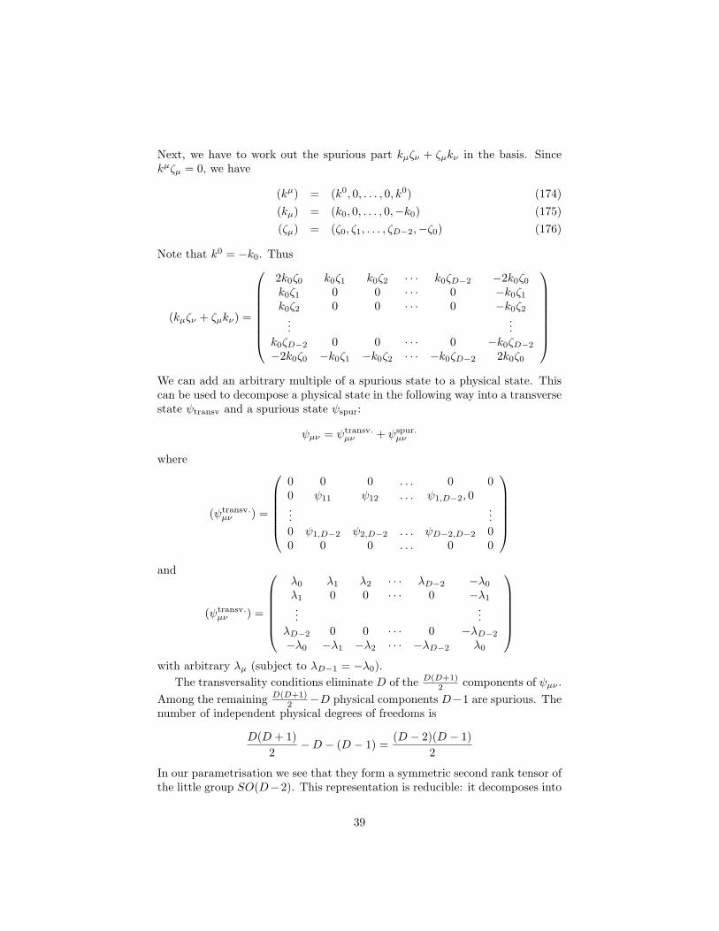
Next, we have to work out the spurious part kµζν + ζµkν in the basis. Sincekµζµ = 0, we have

(kµ) = (k0, 0, . . . , 0, k0) (174)(kµ) = (k0, 0, . . . , 0,−k0) (175)(ζµ) = (ζ0, ζ1, . . . , ζD−2,−ζ0) (176)

Note that k0 = −k0. Thus

(kµζν + ζµkν) =

2k0ζ0 k0ζ1 k0ζ2 · · · k0ζD−2 −2k0ζ0k0ζ1 0 0 · · · 0 −k0ζ1k0ζ2 0 0 · · · 0 −k0ζ2

......

k0ζD−2 0 0 · · · 0 −k0ζD−2

−2k0ζ0 −k0ζ1 −k0ζ2 · · · −k0ζD−2 2k0ζ0

We can add an arbitrary multiple of a spurious state to a physical state. Thiscan be used to decompose a physical state in the following way into a transversestate ψtransv and a spurious state ψspur:

ψµν = ψtransv.µν + ψspur.

µν

where

(ψtransv.µν ) =

0 0 0 . . . 0 00 ψ11 ψ12 . . . ψ1,D−2, 0...

...0 ψ1,D−2 ψ2,D−2 . . . ψD−2,D−2 00 0 0 . . . 0 0

and

(ψtransv.µν ) =

λ0 λ1 λ2 · · · λD−2 −λ0

λ1 0 0 · · · 0 −λ1

......

λD−2 0 0 · · · 0 −λD−2

−λ0 −λ1 −λ2 · · · −λD−2 λ0

with arbitrary λµ (subject to λD−1 = −λ0).

The transversality conditions eliminate D of the D(D+1)2 components of ψµν .

Among the remaining D(D+1)2 −D physical components D−1 are spurious. The

number of independent physical degrees of freedoms is

D(D + 1)2

−D − (D − 1) =(D − 2)(D − 1)

2

In our parametrisation we see that they form a symmetric second rank tensor ofthe little group SO(D−2). This representation is reducible: it decomposes into

39

the trace, which is a scalar, and the traceless part. The traceless, symmetric,second rank tensor representation of the little group has dimension (D−2)(D−1)

2 −1 and is the representation of the D-dimensional graviton.

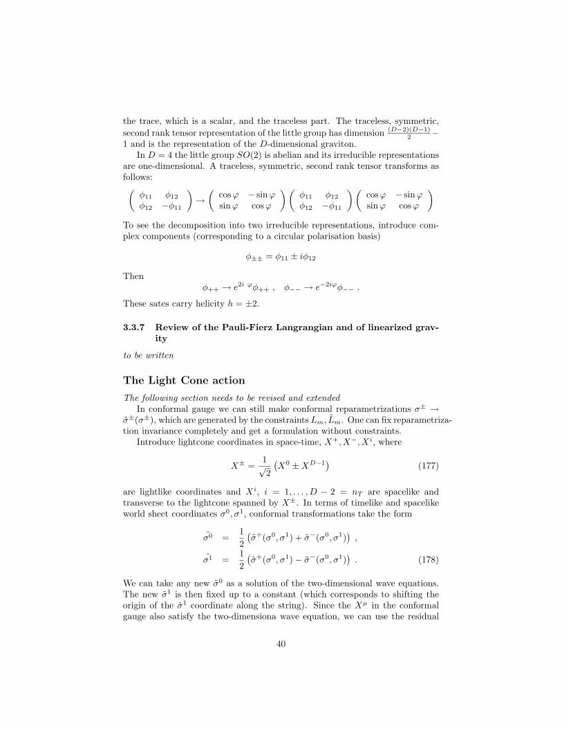
In D = 4 the little group SO(2) is abelian and its irreducible representationsare one-dimensional. A traceless, symmetric, second rank tensor transforms asfollows:(

φ11 φ12

φ12 −φ11

)→(

cosϕ − sinϕsinϕ cosϕ

)(φ11 φ12

φ12 −φ11

)(cosϕ − sinϕsinϕ cosϕ

)To see the decomposition into two irreducible representations, introduce com-plex components (corresponding to a circular polarisation basis)

φ±± = φ11 ± iφ12

Thenφ++ → e2i ϕφ++ , φ−− → e−2iϕφ−− .

These sates carry helicity h = ±2.

3.3.7 Review of the Pauli-Fierz Langrangian and of linearized grav-ity

to be written

The Light Cone action

The following section needs to be revised and extendedIn conformal gauge we can still make conformal reparametrizations σ± →

σ±(σ±), which are generated by the constraints Lm, Lm. One can fix reparametriza-tion invariance completely and get a formulation without constraints.

Introduce lightcone coordinates in space-time, X+, X−, Xi, where

X± =1√2

(X0 ±XD−1

)(177)

are lightlike coordinates and Xi, i = 1, . . . , D − 2 = nT are spacelike andtransverse to the lightcone spanned by X±. In terms of timelike and spacelikeworld sheet coordinates σ0, σ1, conformal transformations take the form

σ0 =12(σ+(σ0, σ1) + σ−(σ0, σ1)

),

σ1 =12(σ+(σ0, σ1)− σ−(σ0, σ1)

). (178)

We can take any new σ0 as a solution of the two-dimensional wave equations.The new σ1 is then fixed up to a constant (which corresponds to shifting theorigin of the σ1 coordinate along the string). Since the Xµ in the conformalgauge also satisfy the two-dimensiona wave equation, we can use the residual

40

parametrization freedom to set σ0 proportional to X+, up to an additive con-stant. This condition defines the light cone gauge:

X+ = x+ + p+σ0 (179)

or α+n = 0 for n 6= 0. In terms of space-time light cone coordinates the con-

straints areX− ±X ′− =

12p+

(Xi ±X ′i)2 . (180)

This can be solved for the α−n :

α−n =1

2p+

nT∑i=1

∑m

αin−mαim (181)

Thus in the light cone gauge only the transverse oscillations αin are independent.In other words the constraints tell us that only transverse oscillations of thestring are physical degress of freedom. We can formulate the theory in terms ofa non-singular, but non-covariant action.

The light cone action is obtained by imposing the gauge and reducing thePolyakov action to the independent, transverse degrees of freedom:

S =T

2

∫d2σ

((Xi)2 − (X ′i)2

). (182)

Equation of motionX −X ′′ = 0 , (183)

where X = (Xi) only contains the transverse modes. Canonical momenta

Π = TX . (184)

Hamiltonian

H =∫ π

0

dσ1(πX − L

)=T

2

∫ π

0

dσ1(X2 +X ′2

)=

Tπ

2

∞∑n=−∞

(αnα−n + αnα−n) = LLC0 + LLC

0 (185)

Dimensional reduction, T-duality and non-abelian gaugesymmetry

to be written

A Literature

• Katrin Becker, Melanie Becker and John H. Schwarz, String Theory andM Theory, A modern introduction (2007).

41

The most recent textbook, attempts to give an introduction from a con-temporary perspective and to treats virtually all recent developments.More advanced than Zwiebach, but according to many colleagues very ac-cessible and not too technical. If you want to have just one book which’covers it all’, this is currently the best choice.

• Barton Zwiebach, A First Course in String Theory (2004).The most accessible textbook. Does not cover advanced or technical as-pects, but includes recent developments such as brane world model build-ing and black hole entropy.

• Joseph Polchinski, String Theory (2 Volumes, 1998).For many the standard textbook. Includes developments of the mid-nineties, such as D-branes. Covers many technical aspects, but is (byopinion of many readers) not detailed enough to learn ’how it’s done’without accompanying lectures or further literature.

• Michael B. Green, John H. Schwarz and Edward Witten, Superstring The-ory (2 volumes, 1987).The classical textbook. Though it does not cover the ’modern stuff’, it isa good reference if you need to know the details of the ’old stuff’.

• Dieter Lust and Stefan Theisen, Lectures on String Theory (1989).Concise, technical exposition of the ’old stuff’. Covers material that is notin Green, Schwarz, Witten. Out of print (I have a copy), and no easy/firstread.

• Thomas Mohaupt, Introduction to String Theory (hep-th/0207249).My humble attempt to summarize some relevant parts of string theory.Reasonably up to date, I hope.

42