Embed Size (px)
Citation preview
Ultracold bosonic atoms
in optical lattices
by
Ana Maria Rey
Dissertation submitted to the Faculty of the Graduate School of theUniversity of Maryland at College Park in partial fulfillment
of the requirements for the degree ofDoctor of Philosophy
2004
Advisory Committee:
Prof. Theodore R. Kirkpatrick, Chairman/AdvisorDr. Charles W. Clark, AdvisorProf. Bei-Lok Hu,Prof. Steve Rolston,Prof. J. Robert Dorfman


There are men who fight one day and are good.There are men who fight one year and are better.
There are some who fight many years and they are better still.But there are some that fight their whole lives,
these are the ones that are indispensable.Berthold Brecht


Abstract
Title of Dissertation: Ultracold bosonic atoms
in optical lattices
Ana Maria Rey, Doctor of Philosophy, 2004
Dissertation directed by: Prof. Theodore R. KirkpatrickPhysicsDr. Charles W. ClarkNational Institute of Standards and Technology
This thesis covers most of my work in the field of ultracold atoms loaded inoptical lattices. It makes a route through the physics of cold atoms in periodicpotentials starting from the simple noninteracting system and going into the many-body physics that describes the strongly correlated Mott insulator regime. Eventhough this thesis is a theoretical work all the chapters are linked either withexperiments already done or with ongoing experimental efforts.
This thesis can be divided into four different parts. The first part compriseschapters 1 to 3. In these chapters, after a brief introduction to the field of opticallattices I review the fundamental aspects pertaining to the physics of systems inperiodic potentials.
The second part deals with the superfluid weakly interacting regime wherestandard mean field techniques can be applied. This is covered in chapters 4 and5. Specifically, chapter 4 introduces the discrete nonlinear Schrodinger equation(DNLSE) and uses it to model some experiments. In chapter 5 I go one stepfurther and include the small quantum fluctuations neglected in the DNLSE bystudying quadratic approximations of the Bose-Hubbard Hamiltonian.
Chapters 6 to 8 can be grouped as the third part of the thesis. In them Iadopt an effective action formalism, the so called two particle irreducible effectiveaction (2PI) together with the closed time path (CTP) formalism to study far-from-equilibrium dynamics. The many-body techniques discussed in these chap-ters systematically include higher order quantum corrections, not included in thequadratic approximations of the Hamiltonian, which we show are crucial for a

correct description of the quantum dynamics outside the very weakly interactingregime.
Finally, chapter 9 to 11 are devoted to study the Mott insulator phase. Inthese chapters using perturbation theory I study the Mott insulator ground stateand its excitation spectrum, the response of the system to Bragg spectroscopy, andpropose a mechanism to correct for the residual quantum coherences inherent tothe Mott insulator ground state. Even though small these are not ideal for the useof neutral atoms in optical lattice as a tool for quantum computation.

Acknowledgements
I want to use this lines to thank and acknowledge all the people that made thisthesis possible.
First and foremost I would like to thank Charles Clark for giving me the in-valuable opportunity to join the NIST group. Through his intelligent ideas, lovefor physics and dedication he gave me not only very good advice and guidancebut also all the encouragement I needed to feel the work I was doing was worth-while and important. It has been a pleasure to work with and learn from such anextraordinary person.
I also want to thank Prof. Ted Kirkpatrick for serving as my University ofMaryland supervisor. He has always made himself available for help and advice.His ideas and suggestions were really valuable for the development of this thesis.
I am also grateful to Prof. Bei Lok Hu. He was an invaluable source of knowl-edge and assistance, especially with regard to the 2PI-CTP formalism discussedin chapters 6 to 8. There has never been an occasion when I’ve knocked on hisdoor and he hasn’t given me time. I cannot leave out Esteban Calzetta and AlbertRoura. Discussions with Bei Lok, Esteban and Albert regarding the applicationof the 2PI-CTP formalism to the patterned loaded system made possible the pub-lication of the paper.
I would also like to acknowledge help and support from Carl Williams. He wasmy other advisor at NIST, willing to help me all the time and providing me withvery useful ideas.
I also owe special gratitude to everybody in the Physics Laboratory at NISTand colleagues in the Radiation Physics Building, in particular Blair Blakie, ZachDutton, Nicolai Nygaard, Marianna Safranova, Jamie Williams and Mark Ed-wards. Besides colleagues they have been wonderful friends and helped me anytime I needed help or advice. Especially I am greatly indebted with Blair whowas not only my office mate when he was at NIST and helped me to sort out allthe problems but also for his support and great ideas even now that he is in NewZealand. I also want to thank Nicolai not only for providing me all the LaTexstyle files for writing this thesis but also for all his time reviewing the manuscript.Guido Pupillo and Gavin Brennen also deserve a special mention. Because of theirgreat ideas and critical thinking the work described in chapters 9 to 11 was possi-ble. I can not forget to thank Prof. Keith Burnett. I worked with him during thesummer of 2002 when he came to NIST. Besides an incredible person, he is alsoa bright physicist. He was the one who gave me the idea of using the superfluid

viii
properties to study the approach to the Mott insulator phase.I owe my deepest thanks to my family - my mother, my father, my sister and
my brother. They have always stood by me in good and bad times. I really oweall my achievements to them.
Finally, I have no words to express the gratitude I have to my husband JuanGabriel. He is the most important person in my life. We came together to pursuethe PhD. program and without his love and support the completion of this workwould not have been possible.

Table of Contents
List of Figures xii
1 Introduction 1
2 Optical lattices 92.1 Basic theory of optical lattices . . . . . . . . . . . . . . . . . . . . 9
2.1.1 AC Stark Shift . . . . . . . . . . . . . . . . . . . . . . . . . 102.1.2 Dissipative interaction . . . . . . . . . . . . . . . . . . . . . 112.1.3 Lattice geometry . . . . . . . . . . . . . . . . . . . . . . . . 12
2.2 Single particle physics . . . . . . . . . . . . . . . . . . . . . . . . . 132.2.1 Bloch functions . . . . . . . . . . . . . . . . . . . . . . . . . 132.2.2 Wannier orbitals . . . . . . . . . . . . . . . . . . . . . . . . 162.2.3 Tight-binding approximation . . . . . . . . . . . . . . . . . 172.2.4 Semiclassical dynamics . . . . . . . . . . . . . . . . . . . . . 19
3 The Bose-Hubbard Hamiltonian and the superfluid to Mott insu-lator transition 253.1 Bose-Hubbard Hamiltonian . . . . . . . . . . . . . . . . . . . . . . 253.2 Superfluid-Mott insulator transition . . . . . . . . . . . . . . . . . 27
4 Mean field theory 314.1 Discrete nonlinear Schrodinger equation (DNLSE) . . . . . . . . . 314.2 Dragging experiment . . . . . . . . . . . . . . . . . . . . . . . . . . 33
4.2.1 Experiment . . . . . . . . . . . . . . . . . . . . . . . . . . . 344.2.2 Linear free particle model . . . . . . . . . . . . . . . . . . . 354.2.3 Effect of the magnetic confinement . . . . . . . . . . . . . . 364.2.4 Interaction effects . . . . . . . . . . . . . . . . . . . . . . . 38
4.3 Dynamics of a period-three pattern-loaded Bose-Einstein conden-sate in an optical lattice . . . . . . . . . . . . . . . . . . . . . . . . 404.3.1 Experiment . . . . . . . . . . . . . . . . . . . . . . . . . . . 424.3.2 Case of no external potential . . . . . . . . . . . . . . . . . 434.3.3 Dynamics with a constant external force . . . . . . . . . . . 51
x TABLE OF CONTENTS
5 Quadratic approximations 615.1 The characteristic Hamiltonian . . . . . . . . . . . . . . . . . . . . 625.2 Bogoliubov-de Gennes (BdG) equations . . . . . . . . . . . . . . . 625.3 Higher order terms . . . . . . . . . . . . . . . . . . . . . . . . . . . 65
5.3.1 Hartree-Fock-Bogoliubov equations . . . . . . . . . . . . . . 665.3.2 HFB-Popov approximation . . . . . . . . . . . . . . . . . . 67
5.4 The Bose-Hubbard model and superfluidity . . . . . . . . . . . . . 675.5 Expectation values . . . . . . . . . . . . . . . . . . . . . . . . . . . 705.6 Applications . . . . . . . . . . . . . . . . . . . . . . . . . . . . . . . 71
5.6.1 Translationally invariant lattice . . . . . . . . . . . . . . . . 715.6.2 One-dimensional harmonic trap plus lattice . . . . . . . . . 78
5.7 Improved HFB-Popov approximation . . . . . . . . . . . . . . . . . 915.7.1 The two-body and many-body scattering matrices . . . . . 925.7.2 The anomalous average and the many-body scattering matrix 935.7.3 Improved Popov approximation . . . . . . . . . . . . . . . . 95
5.8 Conclusions . . . . . . . . . . . . . . . . . . . . . . . . . . . . . . . 99
6 The two particle irreducible effective action (2PI) and the closedtime path (CTP) formalism 1016.1 2PI effective action Γ(z,G) . . . . . . . . . . . . . . . . . . . . . . 1026.2 Perturbative expansion of Γ2(z, G) and approximation schemes . . 107
6.2.1 The standard approaches . . . . . . . . . . . . . . . . . . . 1076.2.2 Higher order expansions . . . . . . . . . . . . . . . . . . . . 1086.2.3 Zero mode fluctuactions . . . . . . . . . . . . . . . . . . . . 109
6.3 CTP formalism . . . . . . . . . . . . . . . . . . . . . . . . . . . . . 1106.4 HFB approximation . . . . . . . . . . . . . . . . . . . . . . . . . . 113
6.4.1 Equations of motion . . . . . . . . . . . . . . . . . . . . . . 1136.4.2 Mode expansion of the HFB equations . . . . . . . . . . . . 114
6.5 Second-order expansion . . . . . . . . . . . . . . . . . . . . . . . . 1166.5.1 Equations of motion . . . . . . . . . . . . . . . . . . . . . . 1166.5.2 Conservation laws . . . . . . . . . . . . . . . . . . . . . . . 123
6.6 Conclusions . . . . . . . . . . . . . . . . . . . . . . . . . . . . . . . 124
7 Nonequilibrium dynamics of a patterned loaded optical lattice:Beyond the mean field approximation 1277.1 Mean field dynamics . . . . . . . . . . . . . . . . . . . . . . . . . . 127
7.1.1 Dynamical evolution . . . . . . . . . . . . . . . . . . . . . . 1287.1.2 Comparisons with the exact solution . . . . . . . . . . . . . 128
7.2 2PI-CTP approximations . . . . . . . . . . . . . . . . . . . . . . . 1317.2.1 Initial conditions and parameters . . . . . . . . . . . . . . 1317.2.2 Numerical algorithm for the approximate solution . . . . . 1327.2.3 Results and discussions . . . . . . . . . . . . . . . . . . . . 133
7.3 Conclusions . . . . . . . . . . . . . . . . . . . . . . . . . . . . . . . 136

TABLE OF CONTENTS xi
8 From the 2PI-CTP approximations to kinetic theories and localequilibrium solutions 1438.1 Rewriting the 2PI-CTP second-order equations . . . . . . . . . . . 1448.2 Boltzmann equations . . . . . . . . . . . . . . . . . . . . . . . . . . 1478.3 Equilibrium properties for a homogeneous system . . . . . . . . . . 152
8.3.1 Quasiparticle formalism . . . . . . . . . . . . . . . . . . . . 1538.3.2 HFB approximation . . . . . . . . . . . . . . . . . . . . . . 1558.3.3 Second-order and Beliaev approximations . . . . . . . . . . 156
8.4 Conclusions . . . . . . . . . . . . . . . . . . . . . . . . . . . . . . . 158
9 Characterizing the Mott Insulator Phase 1599.1 Commensurate translationally invariant case . . . . . . . . . . . . . 159
9.1.1 Perturbation theory . . . . . . . . . . . . . . . . . . . . . . 1599.2 Harmonic confinement plus lattice . . . . . . . . . . . . . . . . . . 1679.3 Conclusions . . . . . . . . . . . . . . . . . . . . . . . . . . . . . . . 171
10 Bragg Spectroscopy 17310.1 Formalism . . . . . . . . . . . . . . . . . . . . . . . . . . . . . . . . 17410.2 Observables . . . . . . . . . . . . . . . . . . . . . . . . . . . . . . . 17610.3 Linear response . . . . . . . . . . . . . . . . . . . . . . . . . . . . . 17710.4 Zero-temperature regime . . . . . . . . . . . . . . . . . . . . . . . . 179
10.4.1 Bogoliubov approach . . . . . . . . . . . . . . . . . . . . . . 17910.4.2 Inhomogeneous system . . . . . . . . . . . . . . . . . . . . . 181
10.5 Mott insulator regime . . . . . . . . . . . . . . . . . . . . . . . . . 18310.5.1 Commensurate homogeneous system . . . . . . . . . . . . . 18410.5.2 Inhomogeneous system . . . . . . . . . . . . . . . . . . . . . 186
10.6 Finite temperature . . . . . . . . . . . . . . . . . . . . . . . . . . . 18810.7 Conclusions . . . . . . . . . . . . . . . . . . . . . . . . . . . . . . . 190
11 Scalable register initialization for quantum computing in an op-tical lattice 19311.1 Homogeneous dynamics . . . . . . . . . . . . . . . . . . . . . . . . 19411.2 Dynamics in presence of the external trap . . . . . . . . . . . . . . 19711.3 Measurement . . . . . . . . . . . . . . . . . . . . . . . . . . . . . . 20111.4 Conclusions . . . . . . . . . . . . . . . . . . . . . . . . . . . . . . . 205
12 Conlusions 207

xii TABLE OF CONTENTS
List of Figures
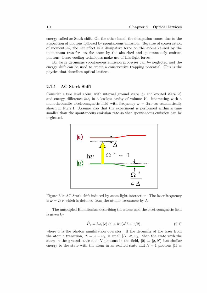
2.1 AC Stark shift induced by atom-light interaction. The laser fre-quency is ω = 2πν which is detuned from the atomic resonance byΛ . . . . . . . . . . . . . . . . . . . . . . . . . . . . . . . . . . . . 10
2.2 Optical lattice potential.(a)-(e) potentials for different configura-tions of 3 beams, (f) potential for the 4 counter-propagating laserbeam configuration (The two pair of light fields are made indepen-dent by detuning the common frequency of one pair of beams fromthe other. ER is the atomic recoil energy, ER = ~2k2/2m. Thisfigure is a courtesy of P. Blair Blakie [34] ) . . . . . . . . . . . . . 14
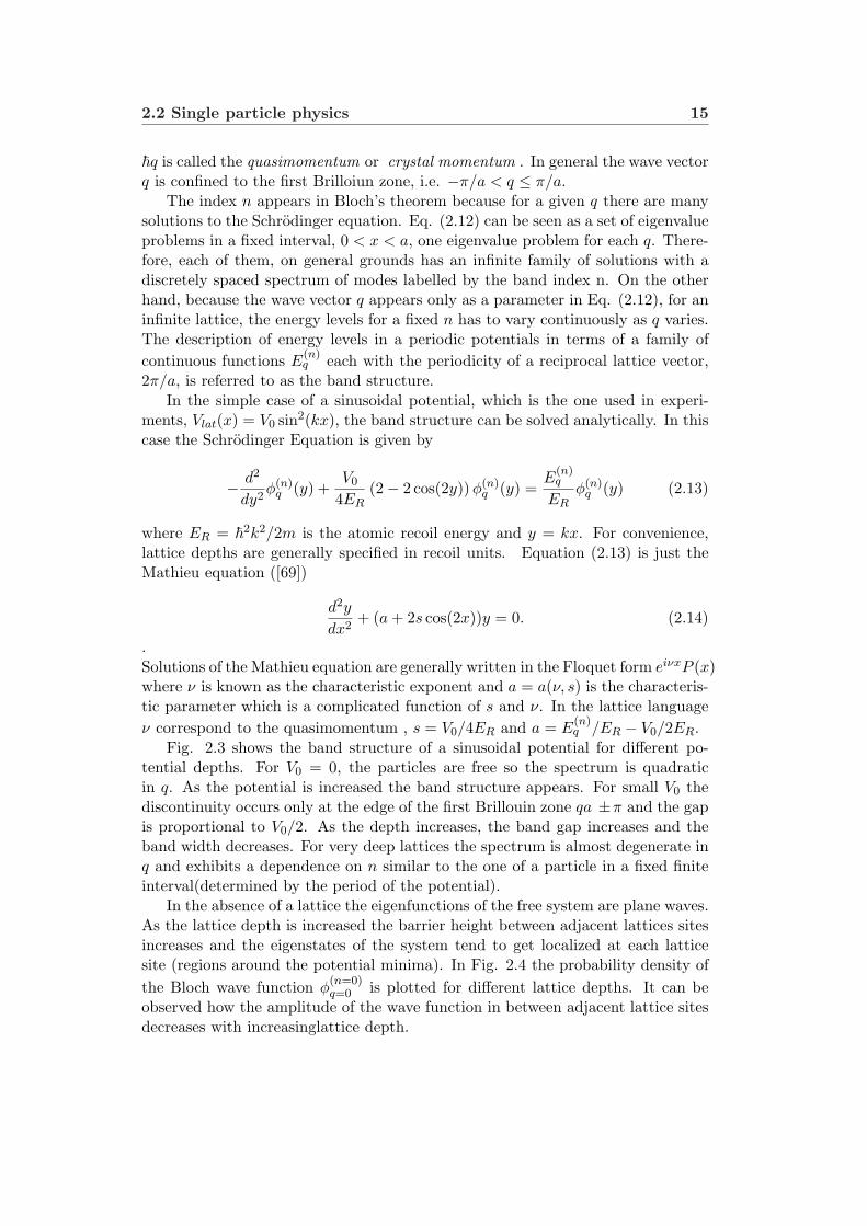
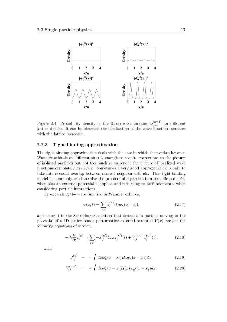
2.3 Band structure of an optical lattice . . . . . . . . . . . . . . . . . . 162.4 Probability density of the Bloch wave function φ
(n=1)q=0 for different
lattice depths. It can be observed the localization of the wave func-tion increases with the lattice increases. . . . . . . . . . . . . . . . 17
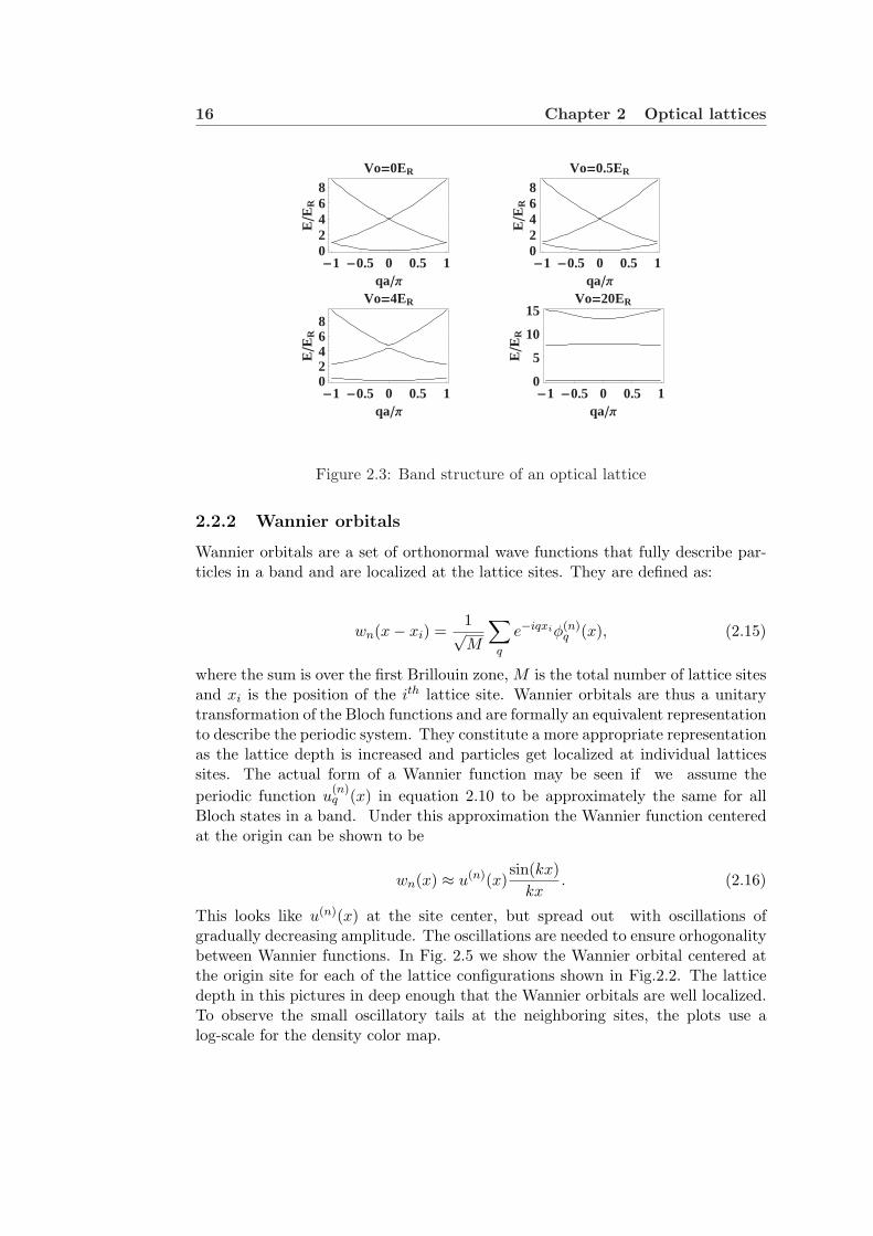
2.5 Wannier state log-density distribution corresponding to the latticeconfigurations shown in Fig. 2.2. Dotted white lines indicate thepotential energy contours. The numbers labels the near neighborsites: 1 the nearest neighbors, and so on. This figure is a courtesyof P. Blair Blakie [34] ) . . . . . . . . . . . . . . . . . . . . . . . . . 18
2.6 Ground state amplitudes f(0)i as a function of the lattice site i for
different values of ξ . . . . . . . . . . . . . . . . . . . . . . . . . . 202.7 Diffusion of a square wave packet in the presence of a linear poten-
tial.The parameters for the plot are ξ = 0.1. . . . . . . . . . . . . . 212.8 Harmonic confinement plus lattice spectrum: The index n labels
the eigenvalues in increasing energy order. . . . . . . . . . . . . . 24
3.1 Zero-temperature phase diagram. The vertical lines indicate criticalvalues for different filling factors . . . . . . . . . . . . . . . . . . . 30
4.1 Condensate density in the x-direction at the observation time tf .Light colors areas indicate regions of high condensate density. Thedashed line indicates the final location of a co-moving point withthe optical lattice. . . . . . . . . . . . . . . . . . . . . . . . . . . . 34

xiv LIST OF FIGURES
4.2 Atom’s average velocity in the lab frame vs. lattice velocity. Line:results from the Bloch dispersion relation, dots: tight-binding ap-proximation results. vB = ~π/am. . . . . . . . . . . . . . . . . . . 36
4.3 Atom’s average velocity in the lab frame vs. lattice velocity in thepresence of a magnetic trap. vB = ~π/am. . . . . . . . . . . . . . . 37
4.4 Velocity of the atoms predicted by the variational model in thecase when interactions are taken into account (dotted line). Thesingle particle case is shown in red. The parameters used wereγ(0) = 10, δ(0) = 0 and NU = 2ER. . . . . . . . . . . . . . . . . . 39
4.5 Phase diagram UN vs vlatt for Vo = 3Er and γo = 10. . . . . . . . 40
4.6 Localization of the wave packet in the self-focusing regime vlatt =−0.7vB. Notice the change in the vertical scale in the last row . . 41
4.7 Evolution of the wave packet in the diffusive regime vlatt = −0.15vB. 41
4.8 Patterned loading experiment. . . . . . . . . . . . . . . . . . . . . . 42
4.9 Oscillation period (in units of ~/J) as a function of the interactionstrength γ. . . . . . . . . . . . . . . . . . . . . . . . . . . . . . . . 45
4.10 Minimum value of f2 during an oscillation period as a function ofγ. As γ increases the population imbalance between wells increases(see text). . . . . . . . . . . . . . . . . . . . . . . . . . . . . . . . 46
4.11 Maximum contrast of the Fourier components as a function of γ.The maximum contrast is defined as ∆max ≡ (|c1|2 − |c0|2)max withthe maximum value occurring when f2 is at its minima. . . . . . 48
4.12 Comparison between the population evolution of the central threewells for the inhomogeneous condensate and the homogeneous model.Inhomogeneous condensate: stars for the initially populated welland boxes for the initially empty wells. Homogeneous model: dashedline represents the initially populated wells, and the solid line rep-resented the initially unpopulated wells. We used γeff as the localmean field energy (see text). The parameters used for the simulationwere J = 0.075ER and γeff = 2.64. . . . . . . . . . . . . . . . . . . 49
4.13 Momentum distribution of the inhomogeneous condensate evaluatedat various times for the same parameters as used in Fig.4.12. . . . 50
4.14 Evolution of momentum peak populations. Upper curves: popula-tion of the q = ±2π/3 momentum states. Lower curves: populationof the q = 0 momentum state. Inhomogeneous condensate (dotted),homogeneous result (solid line), where the comparison is made by re-placing γ by an average mean field energy γave ≡ Λ
∑n |zn|4 = 1.85.
Parameters are the same as in Fig. 4.12. . . . . . . . . . . . . . . 51

LIST OF FIGURES xv
4.15 Evolution of the normalized population for different values of ξ. OneBloch period is shown in the plots except ξ = 0 where the periodis infinite. Solid line: |Ψ3n|2, dotted line: |Ψ3n+1|2, dash-dot line:|Ψ3n+2|2. The ”nonclassical” motion can be seen where the 3n+1-well populations initially increase more rapidly that the populationsof the 3n+2-wells. It can also be seen in the plots that ξ = ξres
max/2and ξ = ξres
max are resonant values. . . . . . . . . . . . . . . . . . . . 55
4.16 The spectrum of values of external force, ordered in decreasing mag-nitude, for which a population resonance occurs i.e. the values of ξfor which Ψ0 periodically disappears. . . . . . . . . . . . . . . . . 56
4.17 Effects of interactions on generalized Bloch oscillations for the pat-tern loaded system. Evolution of |Ψn|2 for various interaction strengths.Upper plot: ξ = 2ξres
max. Lower plot: ξ = 2ξresmax/7. . . . . . . . . . . 57
4.18 Comparison between the evolution of a inhomogeneous condensatewith the homogeneous result. Inhomogeneous condensate: |Ψ0|2(boxes), |Ψ1|2 (stars), and |Ψ2|2 (diamonds). Homogeneous case:|Ψ3n|2 (dash-dot line), |Ψ3n+1|2 (solid line), and |Ψ3n+2|2 (dottedline), where we have taken γ as the local mean field energy. Theparameters used were J = 0.075ER, ξ = 2 and γeff = 1.59 . . . . . 59
4.19 Evolution of the momentum peak populations. q = 0 (dashed line,squares), q = −2π/3 (dash-dot line, stars), q = 2π/3 (solid line, dia-monds). Inhomogeneous condensate (dotted curves), homogeneousmodel (lines) using the same parameters as those in Fig. 4.18, butreplacing γ by an average value γave = 1.11 for the homogeneousmodel. . . . . . . . . . . . . . . . . . . . . . . . . . . . . . . . . . 59
5.1 Scattering processes included in the quadratic hamiltonian: a) Di-rect and exchange excitations, b) Pair excitations . . . . . . . . . . 63
5.2 Comparisons of the exact solution and BdG (and HFB-Popov) so-lutions as a function of Veff = U/J , for a system with M = 3and filling factors n = 5 and 5.33. Left: number fluctuations (Ex-act: solid line, BdG(and HFB-Popov): dotted line), middle: con-densate fraction (Exact: solid line, BdG(and HFB-Popov): dottedline,analytic (5.79:red line ), right: superfluid fraction fs (Exact:solid line, BdG(and HFB-Popov): dotted line). The exact secondorder term (dashed line) of the superfluid fraction, f
(2)s is also shown
in these plots. The vertical line shown in the plots is an estimationof V crit
eff when the system is commensurate . . . . . . . . . . . . . 75
xvi LIST OF FIGURES
5.3 Comparisons of the exact solution and BdG(and HFB-Popov) solu-tions as a function of Veff = U/J , for a system with M = 3 andfilling factors n = 50 and 50.33. Left: number fluctuations (Exact:solid line, BdG(and HFB-Popov): dotted line), middle: condensatefraction (Exact: solid line, BdG(and HFB-Popov): dotted line, ana-lytic Eq.(5.79): red line ), right: superfluid fraction fs (Exact: solidline, BdG(and HFB-Popov): dotted line). The exact second orderterm (dashed line) of the superfluid fraction, f
(2)s is also shown in
these plots. In this case the agreement is much better. . . . . . . 76
5.4 Comparisons of the condensate fraction given by the BdG solutionsand the HFB equations as a function of Veff = U/J , for a systemwith M = 3 and filling factor n = 10. . . . . . . . . . . . . . . . . 78
5.5 Comparisons of the condensate wave function found by numericallysolving the BdG equations with the Thomas-Fermi solution. Theparameters used were U/J = 0.2, Ω/J = 9.5 × 10⁻⁴ and N = 100.The depletion is also shown in the plot. . . . . . . . . . . . . . . . 82
5.6 Comparisons of the quasiparticle spectrum found by numericallysolving the BdG equations(BdG) with the Thomas-Fermi solution(TF) and the noninteracting energies (Free). The parameters usedwere U/J = 0.2, Ω/J = 9.5× 10⁻⁴ and N = 100. . . . . . . . . . 83
5.7 Low-lying quasiparticle amplitudes found by numerically solving theBdG equations. The parameters used were U/J = 0.2, Ω/J =9.5× 10⁻⁴ and N = 100. . . . . . . . . . . . . . . . . . . . . . . . 84
5.8 Comparisons between the product F snGs
n calculated from the Thomas-Fermi approximation and the exact numerical solution of the BdGequations. The parameters used were U/J = 0.2, Ω/J = 9.5× 10⁻⁴
and N = 100. . . . . . . . . . . . . . . . . . . . . . . . . . . . . . 85
5.9 Condensate density (triangles), total density (filled boxes) andlocal depletion (empty diamonds) as a function of the lattice site ifor different values of Veff..The site indices i are chosen such that i =0 corresponds to the center of the trap. Although these quantitiesare defined only at the discrete lattice sites we join them to helpvisualization. The empty boxes represent the exact solution for thecase J=0. . . . . . . . . . . . . . . . . . . . . . . . . . . . . . . . . 86
5.10 Quasiparticle spectrum predicted by the HFB-Popov theory fordifferent values of Veff : Empty diamonds (Veff = 0.01), stars(Veff = 0.09), crosses (Veff = 3), filled diamonds (Veff = 11),empty boxes (Veff = 100) and pentagons (Veff = 312). The letterq labels the quasiparticle energies in increasing order. The quasi-particle energies are in recoil units. . . . . . . . . . . . . . . . . . . 87
LIST OF FIGURES xvii
5.11 Number fluctuations in the self consistent HFB-Popov approach as afunction of lattice site for Veff = 0.01 (boxes), Veff = 0.09 (crosses),Veff = 3 (circles),Veff = 11 (triangles), Veff = 100 (stars) andVeff = 312 (diamonds). The maximum value reached by the pro-file decreases as Veff is increased. The empty boxes shown for eachof the curves correspond to the number fluctuations predicted bythe homogeneous HFB-Popov model using a local density approxi-mation. . . . . . . . . . . . . . . . . . . . . . . . . . . . . . . . . . 88
5.12 Quasimomentum distribution as a function of qa, a the lattice spac-ing, q the quasimomentum, for different values of Veff . . . . . . . . 89
5.13 First order on-site superfluid fraction as a function of the latticesite i for different values of Veff ..The site indices i are chosen suchthat i = 0 corresponds to the center of the trap. Filled boxes: Veff .
=0.01, empty boxes: Veff . = 0.09, empty diamonds: Veff . = 3,stars: Veff . = 11, crosses: Veff . = 100 and triangles: Veff . = 312. . 90
5.14 Diagrammatic representation of the two-body T2b scattering matrix.In this figure |kl〉 designates the initial states, |ij〉 the final statesand |np〉 a set of intermediate states . . . . . . . . . . . . . . . . . 92
5.15 Comparisons of the condensate fraction predicted from the exactdiagonalization of the BHH (red), the improved Popov approxima-tion (yellow), the BdG (and HFB-Popov) equations (blue) and thetest field approximation (green) as a function of Veff = U/J , for asystem with M = 3 and filling factors n = 5 and 5.33. . . . . . . . 97
5.16 Comparisons of the condensate fraction predicted from the exactdiagonalization of the BHH (red), the improved Popov approxima-tion (yellow), the BdG (and HFB-Popov) equations (blue) and thetest field approximation (green) as a function of Veff = U/J , for asystem with M = 3 and filling factors n = 50 and 50.33. . . . . . . 98
5.17 Comparisons between no/nTmb = fcTmb and U as a function of Ufor a system with M = 3 and filling factors n = 5 and 50. . . . . . 98
6.1 Two-loop (upper row) and three-loop diagrams (lower row) con-tributing to the effective action. Explicitly, the diagram a) is whatwe call the double-bubble , b) the setting-sun and c) the basketball. 102
xviii LIST OF FIGURES
7.1 Comparisons between the exact and the DNLSE solutions for sixatoms and three wells. The time is given in units of ~/J . Toppanel, strongly correlated regime (γ = 12); middle panel, inter-mediate regime (γ = 2); bottom panel, weakly interacting regime(γ = 0.2). The solid line is the DNLSE prediction for the populationper well: |z0(t)|2 and |z1,2(t)|2, the triangles are used to representthe exact solution for the population per well calculated using theBose Hubbard Hamiltonian: 〈a†0a0〉, 〈a†1,2a1,2〉. The pentagons showthe condensate population per well calculated from the exact so-lution: |〈a0〉|2 and |〈a1,2〉|2. Due to the symmetry of the initialperiodic conditions the curves for the i = 1 and 2 wells are the samein all depicted curves . . . . . . . . . . . . . . . . . . . . . . . . . . 137
7.2 Comparisons between the exact solution(solid line), the HFB ap-proximation (boxes), the second-order large N approximation (pen-tagons) and the full 2PI second-order approximation(crosses) forthe very weak interacting regime. The parameters used were M =3, N = 6, J = 1 and U/J = 1/30. The time is given in units of~/J . In the plots where the population, condensate and deple-tion per well are depicted the top curves correspond to the initiallypopulated well solutions and the lower to the initially empty wells.Notice the different scale used in the depletion plot. In the momen-tum distribution plot the upper curve corresponds to the k = ±2π/3intensities and the lower one to the k = 0 quasi-momentum intensity. 138
7.3 Comparisons for the case M = 3, N = 8, J = 1 and U/J = 1/3.The time is given in units of ~/J . In the plots the abbreviation 1stis used for the initially occupied well and 2nd for the initially emptywells. In the quasimomentum plots k = 2π/a is the reciprocal latticevector with a the lattice spacing. . . . . . . . . . . . . . . . . . . 139
7.4 Comparison between the evolution of the atomic population perwell for M = 2, J = 1/2, NU/J = 4 and N = 20, 40 and 80. Timeis in units of ~/J . In the plots P1 stands for the fractional atomicpopulation in the initially populated wells and P2 for the populationin the initially empty wells. The number of atoms N is explicitlyshown in each panel. . . . . . . . . . . . . . . . . . . . . . . . . . 140
7.5 Time evolution of the condensate population per well and the totalcondensate population,for the same parameters as Fig. 7.4. Time isin units of ~/J . In the plots C1 stands for the fractional condensatepopulation in the initially populated well, C2 for the fractional con-densate population in the initially empty one and CT for the totalcondensate fraction. . . . . . . . . . . . . . . . . . . . . . . . . . . 141

LIST OF FIGURES xix
7.6 Dynamical evolution of the quasi-momentum intensities. The pa-rameters used were M = 2, J = 1/2, NU/J = 4 and N = 20, 40 and80. Time is in units of ~/J . In the plots ko denotes the k = 0 quasi-momentum component and k1 the k = π/a one (a the lattice spac-ing). The plots are scaled to set the integrated quasi-momentumdensity to one for all N . . . . . . . . . . . . . . . . . . . . . . . . 142
9.1 Contour plot of the two dimensional band of the 1-ph excitationsto fist order in perturbation theory. In the plot the brighter thecolor the higher the energy. The labels are ky = 2π/MR and kx =2π/MR. . . . . . . . . . . . . . . . . . . . . . . . . . . . . . . . . 163
9.2 Comparisons between the first order corrections to the 1-ph exci-tations calculated by diagonalizing the Bose-Hubbard Hamiltonianinside the 1-ph subspace and the analytic solution Eq. (9.22). Thenumber of sites used for the plot was M = 11. Energies are in unitsof J. . . . . . . . . . . . . . . . . . . . . . . . . . . . . . . . . . . . 164
9.3 Comparisons between the energy eigenvalues calculated by the exactdiagonalization of the Hamiltonian (red dots), the diagonalizationof the Hamiltonian in the restricted 1-ph subspace (green triangles)and the analytic solution (blue crosses), Eq. (9.22). The indexn labels the eigenvalues in increasing order of energy. The fillingfactor g, the number of wells M and the ratio U/J is indicated ineach plot. Energies are in units of J. . . . . . . . . . . . . . . . . . 165
9.4 Quasimomentum distribution as a function of U/J for a unit filledlattice with six wells (M = 6). The exact solutions are displayedwith solid lines and the first order perturbative results with dottedlines. Due to the lattice symmetry n4π/3 = n2π/3 and n5π/3 = nπ/3. 166
9.5 Comparisons between the exact (red) and the perturbative (blue)spectra for a trapped system with N = 9, M = 11 and Ω/J = 1.875deep in the Mott regime. The lines indicate the energies of thestates that are coupled directly to the ground state. . . . . . . . . 170
10.1 Bragg spectroscopic scheme considered in this paper. The latticepotential with atoms loaded into the ground band is perturbed bya shallow running wave perturbation (the Bragg potential). . . . . 174
10.2 Imparted energy: Comparisons between the the exact and Bogoli-ubov approximation for N = M = 9. The horizontal axis is in unitsof ~. For the plot we used Jτ/~ = 10. See text Eq. (10.23). . . . . 181
10.3 Comparisons of the imparted energy vs. Bragg frequency curvescalculated from the exact diagonalization of the manybody Hamil-tonian (red) and the from the HFB-Popov approximation(blue) fora trapped system with N = 9, M = 11 and Ω/J = 1.875. Thehorizontal axis is in units of ~. The lines depicted in the plot arelocated at the different quasiparticle energies excited by the Braggperturbation. . . . . . . . . . . . . . . . . . . . . . . . . . . . . . . 183
xx LIST OF FIGURES
10.4 Density profile calculated from the exact diagonalization of themany-body Hamiltonian (red) and from the HFB-Popov approx-imation (blue) for a trapped system with N = 9, M = 11 andΩ/J = 1.875. n labels the lattice site. . . . . . . . . . . . . . . . . 184
10.5 Dynamical structure factor vs. ~ω/J in the Thomas-Fermi (blue)and HFB-Popov (red) approximations. The horizontal axis is inunits of ~. The system parameters are U/J = 0.2, Ω/J = 9.5×10⁻⁴
and N = 100. . . . . . . . . . . . . . . . . . . . . . . . . . . . . . 185
10.6 Eigenvalues of the quasiparticle spectrum plotted in increasing en-ergy order. The vertical scale is in units of ~ . . . . . . . . . . . . 186
10.7 Transfer energy vs. Bragg frequency for a zero temperature homo-geneous system with M = N = 9 and different transfer momentaq. The horizontal axis is in units of ~. The perturbation time wasset to Jτ/~ = 10. Note the change of the vertical scale between thetwo panels. . . . . . . . . . . . . . . . . . . . . . . . . . . . . . . . 186
10.8 Transfer energy vs. Bragg frequency for a zero temperature trappedsystem with parameters U/J=45, Ω/J = 1.857, M = 11 and N = 9and different transfer momenta q. The horizontal axis is in units of~. The perturbation time was set to Jτ/~ = 10. Note the changeof the vertical scale between the two panels. . . . . . . . . . . . . 187
10.9 Transfer energy as a function of the temperature for different U/Jparameters. The plots are for a homogeneous system with N =M = 9. The horizontal axis in in units of ~. . . . . . . . . . . . . 191
10.10Transfer energy as a function of the temperature for different U/Jparameters. The plots are for an trapped system with M = 11,N = 9 and Ω/J = 1.875. The horizontal axis in in units of ~. . . . 192
11.1 Comparisons between the time evolution of the percentage fidelitycalculated by diagonalizing the Bose-Hubbard Hamiltonian (dots),the perturbative solution inside the one particle hole subspace (red)and the analytic solution Eq. 11.6 (blue). . . . . . . . . . . . . . . 196
11.2 Percentage fidelity as a function of time calculated using the per-turbative solution 11.4 (red) and the analytic solution Eq. 11.6(blue).The number of sites used for the plot is M = 31 . . . . . . 197
11.3 Schematic of an inhomogeneous lattice filled with N qubits with anonsite interaction energy U . An externally applied trapping poten-tial of strength Vj = Ωj2, e.g. due to a magnetic field, acts to fillgaps in the central region of the trap. The center subspace R of thelattice defines the quantum computer register containing K < Nqubits. . . . . . . . . . . . . . . . . . . . . . . . . . . . . . . . . . . 198

LIST OF FIGURES xxi
11.4 Comparisons between the time evolution of the percentage fidelityFcom(K = 5, t) calculated by evolving the initial target state usingthe Bose-Hubbard Hamiltonian (dots), the restricted one particlehole basis (red) and the analytic solution Eq. 11.16 (blue). In theplot we assumed a commensurate unit filled lattice with five sitesand infinitely high boundaries. . . . . . . . . . . . . . . . . . . . . 200
11.5 Percentage fidelity as a function time calculated using the approx-imated solution 11.16 (blue) and the fidelity found numerically byrestricting the dynamics to the one particle hole subspace. We as-sumed infinity high boundaries and K = 31. . . . . . . . . . . . . 201
11.6 Schematic of the relevant couplings in the problem. The unit filledstate |T 〉 describing a target quantum register and the states |S±j 〉having one doubly occupied lattice site and a neighboring hole arecoupled to first order in J . A catalysis laser resonantly couples theground states |S±j 〉 to the excited states |M±
j 〉 describing a boundmolecule at the doubly occupied site. The bound states quickly de-cay and give the possibility of monitoring population in the “faulty”register states |S±j 〉. . . . . . . . . . . . . . . . . . . . . . . . . . . 202
11.7 Population in the unit filled register state |T 〉R during continuousmeasurement of the register beginning in the Bose-Hubbard groundstate |Ψg〉. The plots show dynamics appropriate to tunneling inone dimension with U/J = 500. (a) Quantum trajectories corre-sponding to a null measurement result for three different registersizes K. The time scale to saturate the target state is independentof the number of qubits: tsat ≈ κ−1. (b) Long time dynamics forK = 501, N = 551 and finite detector efficiencies η. The popula-tion in |T 〉R for η = 1 is indistinguishable from one. Also shown isthe oscillatory dynamics at fundamental frequency U described byEq. (11.16) if the measurement is turned off after the target stateis reached. The arrow indicates ρT,T (0). . . . . . . . . . . . . . . . 203
Chapter 1
Introduction
Bose Einstein condensation (BEC) in bosonic gases was predicted by Einstein in1925 [1] based on the quantum statistics ideas developed by Bose for photons [2].The basic idea of BEC is that below a critical temperature a macroscopic numberof particles occupy the lowest energy state: as the temperature, T, is decreased thede-Broglie wave length, which scales like T−1/2, increases and at the critical point itbecomes comparable to the inter-particle mean separation. At this point the wavefunctions of the particles are sufficiently smeared out so that there is always someoverlap and a Bose Einstein condensate is formed. Although Einstein’s predictionapplied to a gas of noninteracting atoms, London suggested that, BEC could bethe mechanism underlying the phenomenon of superfluidity in 4He [3], despite thestrong interactions in this system. Further evidence for this point of view camefrom neutron scattering experiments [4].
Experimental efforts to create a BEC in dilute gases date back to the 1980’s[5]. The first experiments concentrated on using atomic Hydrogen but mainly thelarge rates of inelastic collision prevented these experiments from succeeding. Itwas not until 1995, using the advances made in laser cooling techniques[9], thatBEC in dilute alkali atomic gases was achieved. The first series of experiments weredone with Rubidium [6], sodium [7] and lithium [8] vapors. In these experimentsatoms are typically collected in a magneto-optical trap (MOT) and compressedand cooled to micro-Kelvin temperatures using laser cooling techniques. They arethen transferred to a magnetic trap where evaporative cooling allows the systemto be cooled to nano-Kelvin temperatures. At a critical phase space density BECtakes place. In such a condensate a macroscopic number of atoms, generally up to106, collectively occupy the lowest energy state.
The experimental realization of BEC in alkali gases opened unique opportu-nities for exploring quantum phenomena on a macroscopic scale. In contrast toexperiments with liquid helium, where the strong interactions between particleswash out the effects due to the BEC, the relatively weak two-particle interactionin dilute alkali atoms allows these systems to be used as a theoretical and experi-mental arena to study coherent matter wave properties. Theoretically, the weaklyinteracting regime has the advantage that all the atoms can be described by a
2 Chapter 1 Introduction
single macroscopic wave function. This allows a very intuitive understanding ofthe system based on the so called Gross-Pitaevskii equation (GPE) [10]. Experi-mentally, the macroscopic wave packet can be probed by interference experiments,where by turning off the trapping fields the atoms are allowed to expand and thewave packets to interfere with each other.
The GPE assumes that all the atoms are in the condensate and neglects com-pletely quantum correlations. In the weakly interacting regime, a description be-yond the simplest mean field theory can be made by treating the small quantumfluctuations as perturbations. This treatment was proposed by Bogoliubov in 1947[11]. The fluctuations lead to a small depletion of the condensate mode since otherexcited states different from the condensate get populated. Since in most of theexperiments with dilute gases the condensate depletion is at most 3%, the GPEtogether with Bogoliubov analysis have been in general very successful describingthese experiments. Much theoretical and experiment work has been done studyingcondensate properties such as condensate collective excitations, phonon modes,sound velocity and superfluid flow phenomena [12]-[19].
However, weakly interacting dilute gases described by a mean field pictureare the simplest many body systems one can possible found. In order to be in theweakly interacting regime, the ratio between the interaction energy of uncorrelatedatoms at a given density, Eint, and the quantum kinetic energy needed to correlateparticles by localizing them within a distance of order of the mean inter-particledistance, Ekin, must be small. For three dimensional systems Eint ∼ n4π~2as
m (as isthe scattering length, which fully characterizes the low energy scattering processes,n is the mean particle density and m is the atomic mass) and Ekin ∼ ~2
2mn2/3.Thus, the ratio between these two energies is proportional to n1/3as. In dilutealkali vapors this ratio is generally of order 0.02. To enter the strongly correlatedregime, an obvious way to proceed is either to raise the density or to raise thescattering length. It is indeed possible to tune the scattering length to large valuesby using a Feshbach resonance. This has recently been realized for example in 85 Rbwhere the scattering length was tuned over several orders of magnitude [20, 21].The problem of this approach is, however, that the lifetime of the condensatestrongly decreases due to three-body losses [22]. An entirely different way to reachthe strongly correlated regime is by using optical lattices. By increasing the depthof the optical lattice the ratio between kinetic energy and potential energy can bechanged without affecting the density or the scattering length. The beauty of thisapproach is that the lattice depth can be used as an experimental knob to changethe kinetic to interaction energy ratio allowing us to reach different many-bodyregimes.
• Optical lattices
Optical lattices are periodic Stark shift potentials created by the interferenceof two or more laser beams. They have been widely used in atomic physics inthe context of atom diffraction [23, 24] with applications to atom optics and atominterferometry [25]. They have also been used as a way to trap and cool atoms. The
3
first experiment where atoms were cooled to the micro-kelvin regime in a multi-dimensional optical lattice was carried out by Hemmerich et al. [26]-[28] followedby Grynberg et al. [29]. There have been various attempts to cool atoms directlyin an optical lattice. Among them we can mention Raman cooling techniques, bywhich atoms have recently been partially cooled to the ground sate with fillingfactors of order one [30, 31, 32]. However, one of the most successful techniquesto load ultracold atoms in the ground state, with almost no discernible thermalcomponent, is by first forming a Bose Einsten condensate in a weak magnetic trapand then adiabatically turning on the lattice by slowly ramping up the intensityof the laser beams.
Atom dynamics in optical lattices is closely related to electron dynamics insolid state crystals, but optical lattice have favorable attributes such as the absenceof defects and the high degree of experimental control [33, 34]. When ultracoldbosonic atoms are loaded in shallow lattices, the system is in the weakly interactingregime and most of the atoms are Bose condensed. Combined with BEC, theultimate source of coherent atom , optical lattices provide a way of exploringa quantum system analogous to electrons in crystals but with complete controlover the lattice and the atoms. Beautiful experiments have been done in thisregime and have provided an elegant demonstration of band structure [35, 36,37], Bragg scattering and Bloch oscillations [38], as well as coherent matter waveinterferometry [39, 40], superfluidity [41] and quantum chaos [42].
There has also been spectacular recent experimental progress in the stronglycorrelated regime. It was first realized by Jaksch et al. [43], that a BEC loaded ina lattice potential is a nearly perfect experimental realization of the Bose-HubbardHamiltonian, which describes bosons with local repulsive interactions in a periodicpotential. M.P.A. Fisher et al. [44] predicted that a system modeled by theBose-Hubbard Hamiltonian exhibits a quantum phase transition from a superfluidto an insulator state (superfluid-Mott insulator transition) as the interactions areincreased. In fact, the Mott insulator transition in a 3D lattice starting from a BEChas experimentally observed by M. Greiner and coworkers [46]. Moreover, in recentyears there have been many impressive experiments which have demonstrated theloss of quantum coherence as the system approaches the strongly correlated regime,for example by measuring number squeezing [45] or by studying the collapse andrevival of coherence in a matter wave field [47].
One of the most important potential applications of the Mott insulator tran-sition is to use it as a mean to initialize a quantum computer register. Deep inthe Mott insulator regime the kinetic energy is very small with respect to the in-teraction energy and it is energetically favorable for the atoms to remain localizedwithout tunneling. The negligible number fluctuations makes it possible to preparethe fiducial state with exactly one atom per site needed to initialize a quantumcomputer register [43, 48, 50]. Besides the possibility of high fidelity initialization,the easy scalability, low noise and high experimental control make ultracold neu-tral atoms loaded in an optical lattice one of the most attractive candidates forimplementations of quantum computation.
4 Chapter 1 Introduction
The overall goal of this thesis is to study equilibrium and non equilibrium prop-erties of cold bosons loaded in optical lattices starting from the superfluid regime,where mean field techniques can be applied, and going into the rich and complexstrongly correlated regime where the standard GPE and Bogoliubov treatmentsfail to describe the system and a more general framework is required. Most of thework is done in the context of ongoing experimental efforts, especially the onestrying to achieve lattice based quantum information processing.
• Overview
In chapter 2, I start by reviewing the theory of optical potentials, the singleparticle band structure and the tight binding approximation. In chapter 3, I goone step further and consider the many-body properties of the system by intro-ducing the Bose-Hubbard Hamiltonian. I give a review of the generic issues thatcharacterize the superfluid to Mott insulator transition.
In chapter 4, I describe the equilibrium properties of lattice systems in thesuperfluid regime, where a mean field treatment is valid. I study the mean fieldDiscrete Nonlinear Schrodinger equation (DNLSE), and use it to model two exper-iments done by the laser-cooling and trapping group at NIST. In the first one, anoptical lattice was moved and the average displacement of the atoms was used asa means to probe the band structure of the system. In the second experiment,towhich I refer as the patterned loading experiment [33],the atoms were loaded intoevery third site of an optical lattice, with the aim of having large enough spatialseparation to address individual atoms. This patterned loading method may bea useful technique for the implementation of lattice based quantum computingproposals.
The DNLSE completely neglects quantum fluctuations. However, if the sys-tem is weakly interacting, the small quantum corrections can be included by usingthe Bogoliubov approximation. In the Bogoliubov approximation the complicatedmany-body quartic Hamiltonian is reduced to a quadratic one, which can be diago-nalized exactly. Using the Bogoliubov approximation, in chapter 5 I study differentstandard quadratic approximations in two different lattice systems, a translation-ally invariant one with periodic boundary conditions which in general allows ana-lytic solutions, and a system closer to real experimental situations where, besidesthe lattice potential, there is a superimposed harmonic confinement potential. Idiscuss the Bogoliubov de Genes equations (BdG), the Hartree-Fock-Bogoliubov(HFB) approximation and the HFB-Popov approximation. To test the validity ofthe different approximations and their departure from the exact solution as theinteractions are increased I compare them with the exact numerical diagonaliza-tion of the Bose-Hubbard Hamiltonian. Because of the exponential scaling of thedimensionality of the Hilbert space with respect to system size, the exact solu-tion (for a system with N atoms and M wells the number of states scales like(N + M − 1!)/(N !M !)), the numerical comparisons are restricted to systems witha moderate number of atoms and wells.
In chapter 5, I also report on our idea of using the superfluid fraction to study
5
the approach to the Mott insulator transition. By deriving an expression forthe superfluid density based on the rigidity of the system under phase variationswe were able to explore the connection between the quantum depletion of thecondensate and the quasi-momentum distribution on one hand and the superfluidfraction on the other.
At the end of the chapter, I present my attempt to approach the stronglycorrelated regime by using the improved Popov approximation [52, 53, 55]. Theidea presented here is to upgrade the bare potential, which is the one that explicitlyappears in the many-body Hamiltonian, to the many-body scattering matrix. Byupgrading the bare potential, we are properly taking into account the effect of thesurrounding atoms in the properties of binary collisions.
In chapter 6 and 7, motivated by the patterned loading experiment, we adopta functional effective action approach capable of dealing with non equilibriumsituations that require a treatment beyond mean field theory. Even though a de-scription of the dynamics of the patterned loading system using the DNLSE wasderived in chapter 4, it is shown by comparisons with the exact quantal solutioncalculated by time propagating the initial configuration with the Bose-HubbardHamiltonian that a mean field solution is valid only for short times and in the veryweakly interacting regime. To deal with the dynamics far from equilibrium, weadopt a closed time path (CTP) [56] functional-integral formalism together witha two-particle irreducible (2PI) [57] effective action approach and derive equationsof motion. We retain terms of up to second-order in the interaction strength whensolving these equations. Under the 2PI-CTP scheme we consider three differentapproximations : a) the time dependent Hartree-Fock-Bogoliubov (HFB) approx-imation, b) the next-to-leading order 1/N expansion and c) a full second-orderperturbative expansion in the interaction strength. We derive mathematical ex-pressions for the equations of motion in chapter 6 and apply them to the particularcase of the patterned loaded lattice in chapter 7. We use this system to illustratemany basic issues in nonequilibrium quantum field theory, such as non-local andnon-Markovian effects, pertaining to the dynamics of quantum correlation andfluctuations. We show that because the second-order 2PI approximations includemulti-particle scattering in a systematic way, they are able to capture dampingeffects exhibited in the exact solution, which a collisionless approach fails to pro-duce. While the second-order approximations show a clear improvement over theHFB approximation, they fail at late times, when interaction effects are significant.
The 2PI effective action formalism provides a useful framework where the meanfield and the correlation functions are treated on the same self-consistent footing.However, it yields dynamical equation of motion that are non local in time andhard to estimate analytically. The idea in chapter 8 is to simplify the 2PI equationsand to obtain near equilibrium solutions where, kinetic theories that describe ex-citations in systems close to thermal equilibrium are valid. In particular, we showin this chapter how the full second-order 2PI equations are in agreement with cur-rent kinetic theories [15],[58]-[62] and reproduce in equilibrium the higher orderperturbative corrections well known in the literature since Beliaev’s work [63].

6 Chapter 1 Introduction
In chapter 9, I jump into the Mott insulator phase and I study the physicalproperties of the system deep in the Mott insulator regime, which is the otherregime where an analytic treatment based on perturbation theory is possible. Aperturbative analysis should be applicable to study current experiments [64] thatreach the strong Mott regime. I derive expressions for the excitation spectrum ofthe Mott state for both homogeneous and trapped systems and compare them withthe solutions obtained by exact diagonalization of the Bose-Hubbard Hamiltonian.The main purpose of this chapter is to understand the many-body properties ofthe Mott insulator ground state and the nature of its many-body excitations whichwill be crucially important as more elaborate experiments with optical lattices inthe strongly correlated regime are undertaken.
One key piece of evidence for the Mott insulator phase transition is the loss ofglobal phase coherence of the matter wavefunction when the lattice depth increasesbeyond a critical value [46]. However, there are many possible sources of phasedecoherence in these systems. It is known that substantial decoherence can beinduced by quantum or thermal depletion of the condensate during the loadingprocess, so loss of coherence is not a proof that the system resides in the Mottinsulator ground state. Indeed, for this reason, in the experiments by Greiner etal. [46] a potential gradient was applied to the lattice to show the presence ofa gap in the excitation spectrum. In chapter 10, we show that another commonexperimental technique, Bragg spectroscopy [65, 66], not only can identify theexcitation gap that opens up in the Mott regime, but also can be used to mapout the excitation spectrum and to determine the temperature of the system whenit is deep in the Mott regime. Specifically, we study the total momentum andtotal energy deposited in the system by the Bragg perturbation calculated undera linear response analysis and obtain analytical solutions in the superfluid anddeep Mott insulator regimes. We test the accuracy of the approximations andtheir deviation from the full quantal behavior as usual by comparing them withnumerical solutions obtained by diagonalizing the Bose-Hubbard Hamiltonian fora moderate number of atoms and wells.
All of the proposals for quantum computation which utilize a lattice-type ar-chitecture have the Mott insulator transition as the initialization scheme to loadexactly one atom per lattice site. Such architecture requires a lattice commensu-rately filled with atoms, which does not correspond exactly to the ground Mottinsulator state. The ground state has a remaining coherence proportional to thetunneling matrix element. This degrades the initialization of the quantum com-puter register and can introduce errors during error correction. I finish this thesiswith chapter 11, where I report on our proposal to solve this problem by using thespatial inhomogeneity created by a quadratic magnetic trapping potential togetherwith a continuous measurement procedure which projects out the components ofthe wave function with more than one atom in any well.

7
Publications in the PhD work:
• Chapter 4
Dynamics of a period-three pattern loaded Bose-Einstein condensate in anoptical lattice, A. M. Rey, P. B. Blakie, Charles W. Clark, Phys. Rev.A 67, 053610 (2003).
• Chapter 5
Bogoliubov approach to superfluidity of atoms in an optical lattice, Rey AM,Burnett K, Roth R, Edwards M, Williams CJ, Clark CW, J. Phys. B:At. Mol. Opt. Phys, 36 , 825 (2003).
• Chapter 6 and 7
Nonequilibrium Dynamics of Optical Lattice - Loaded BEC Atoms: BeyondHFB Approximation, A. M. Rey, B. L. Hu, E. Calzetta, A. Roura,Charles W. Clark, Phys. Rev A. 69, 033610 (2004).
BEC with fluctuations: beyond the HFB approximation, A. M. Rey, B. L.Hu, E. Calzetta, A. Roura, Charles W. Clark (Proceedings of the LaserPhysics Workshop 2003), Las. Phys., 14, 1, (2004).
• Chapter 10
Bragg spectroscopy of ultracold atoms loaded in an optical lattice, Ana MariaRey, P. Blair Blakie, Guido Pupillo, Carl J. Williams, Charles W. Clark,submitted to Phys. Rev. Lett. cond-mat/0406552.
• Chapter 11
Scalable register initialization for quantum computing in an optical lattice,G. K. Brennen, G. Pupillo, A. M. Rey, C. W. Clark, C. J. Williams,submitted to Phys. Rev. Lett., cond-mat/0312069.
Scalable quantum computation in systems with Bose-Hubbard dynamics,Guido Pupillo, Ana M. Rey, Gavin Brennen, Carl J. Williams, CharlesW. Clark, to appear in J. Mod. Opt, quant-ph/0403052.

8 Chapter 1 Introduction

Chapter 2
Optical lattices
Optical lattices are periodic potentials created by light-matter interactions. Whenan atom interacts with an electromagnetic field, the energy of its internal statesdepends on the light intensity. Therefore, a spatially dependent intensity inducesa spatially dependent potential energy. If such a modulation is obtained by theinterference of several laser beams, the resultant optical potential felt by the atomswill have different potential wells separated by a distance of the order of the laserwavelength. The depths of the optical potential wells that can be obtained in anexperiment are in the microKelvin range. Nevertheless, atoms can be trapped inthis potentials when cooled at low temperatures, by laser and evaporative coolingtechniques.
Cold atoms interacting with a spatially modulated optical potential resemblein many respects electrons in ion-lattice potential of a solid crystals . However,optical lattices have several advantages with respect to solid state systems. Theycan be made to be largely free from defects, such defects for example prevented theobservation of Bloch oscillations in crystalline solids. Optical lattices also can becontrolled very easily by changing the laser field properties. For example the latticedepth can be changed by modifying the laser intensity, the lattice can be movedby changing the polarization of the light or chirping the laser frequency and thelattice geometry can be modified by changing the laser configuration. Moreover,in contrast to solids, where the lattice spacings are generally of order of Angstromunits, the lattice constants in optical lattices are typically three order of magnitudelarger.
The idea of this chapter is to introduce the basic theory of optical lattices andto review the single particle properties of atoms loaded in such periodic potentials.
2.1 Basic theory of optical lattices
Neutral atoms interact with light in both dissipative and conservative ways.The conservative interaction comes from the interaction of the light field withthe induced dipole moment of the atom which causes a shift in the potential
10 Chapter 2 Optical lattices
energy called ac-Stark shift. On the other hand, the dissipation comes due to theabsorption of photons followed by spontaneous emission. Because of conservationof momentum, the net effect is a dissipative force on the atoms caused by themomentum transfer to the atom by the absorbed and spontaneously emittedphotons. Laser cooling techniques make use of this light forces.
For large detunings spontaneous emission processes can be neglected and theenergy shift can be used to create a conservative trapping potential. This is thephysics that describes optical lattices.
2.1.1 AC Stark Shift
Consider a two level atom, with internal ground state |g〉 and excited state |e〉and energy difference ~ωo in a lossless cavity of volume V , interacting with amonochromatic electromagnetic field with frequency ω = 2πν as schematicallyshown in Fig.2.1. Assume also that the experiment is performed within a timesmaller than the spontaneous emission rate so that spontaneous emission can beneglected.
Figure 2.1: AC Stark shift induced by atom-light interaction. The laser frequencyis ω = 2πν which is detuned from the atomic resonance by Λ
The uncoupled Hamiltonian describing the atoms and the electromagnetic fieldis given by
Ho = ~ωo |e〉 〈e|+ ~ω(a†a + 1/2), (2.1)
where a is the photon annihilation operator. If the detuning of the laser fromthe atomic transition, ∆ = ω − ωo, is small |∆| ¿ ωo, then the state with theatom in the ground state and N photons in the field, |0〉 ≡ |g,N〉 has similarenergy to the state with the atom in an excited state and N − 1 photons |1〉 ≡

2.1 Basic theory of optical lattices 11
|e,N − 1〉 , E1 − E0 = −~∆. The effect of the interactions is to couple thesestates. Under the dipole approximation which assumes that the spatial variationof the electromagnetic field is small compared with the atomic wave function, thecoupling Hamiltonian denoted as HI in the interaction picture is given by:
HI = −~d · ~E (2.2)
=(|e〉 〈g| eiωot + |g〉 〈e| e−iωot
) (~Ω∗(~x)
2a†eiωt +
~Ω(~x)2
ae−iωt
).
Here Ω(x) is the Rabi frequency given by ~Ω(~x) = −2√~ω〈N〉2∈V u(~x)~ε · ~d, with ~ε the
unit polarization vector of the field, ~d the dipole moment of the atom and u(~x)the field mode evaluated at the atomic position x,(for plane waves, for exampleu(~x) = e−i~k·~x). In the rotating wave approximation, valid in the limit |∆| ¿ ωo, thetype of processes with a rapidly oscillating phase, exp(±i(ωo + ω)t), are neglectedand only the near resonant frequency processes are considered. The interactionHamiltonian is then reduced to
HI ≈(~Ω(~x)
2|e〉 〈g| aei∆t +
~Ω∗(~x)2
|e〉 〈g| a†e−i∆t
). (2.3)
Physically, the resonant process correspond to either the excitation of the atomalong with the emission of a photon or the relaxation of the atom with the absorb-tion of a photon. In the previous line we also assume a large number of photonsand neglect the variation in the coupling constant due to ∆N, i.e N ' N − 1.
If the detuning is large compared to the Rabi frequency, |∆| À Ω, the effectof the interactions on the states, |0〉 and |1〉, can be determined with second orderperturbation theory. In this case, the energy shift E
(2)0,1 is given by
E(2)0,1 = ±| 〈1| Hint |0〉 |2
~∆= ±~ |Ω(~x)|2
4∆, (2.4)
with the plus and minus sign for the |0〉 and |1〉 states respectively. This energyshift is the so called ac-Stark shift. Since the atoms are practically always in theground state, the energy of the atoms is changed according to the stark shift~ |Ω(~x)|2
4∆ , which defines the optical potential.Furthermore, if instead of interacting with a monochromatic electromagnetic
field, the atoms are illuminated with superimposed counter-propagating laser beams,the beams interfere and the interference pattern results in a periodic landscape po-tential or optical lattice.
2.1.2 Dissipative interaction
In the above discussion we implicitly assumed that the excited state has an infinitelifetime. However, in reality it will decay by spontaneous emission of photons. This

12 Chapter 2 Optical lattices
effect can be taken into account phenomenologically by attributing to the excitedstate an energy with both real an imaginary parts. If the excited state has a lifetime 1/Γe corresponding to a e-folding time for the occupation probability of thestate, the corresponding life time for the amplitude will be twice this time. Theenergy of the perturbed ground state becomes a complex quantity which we canwrite as
E(2)0 =
~4
|Ω(~x)|2∆− iΓe/2
= V (~x) + iγsc(~x), (2.5)
V (~x) = ~|Ω(~x)|2∆4∆2 − Γ2
e
≈ ~ |Ω(~x)|24∆
, (2.6)
γsc(~x) =~2|Ω(~x)|2Γe
4∆2 − Γ2e
≈ ~ |Ω(~x)|2Γe
8∆2. (2.7)
The real part of the energy corresponds to the optical potential whereas the imag-inary part represents the the rate of loss of atoms from the ground state. The signof the optical potential seen by the atoms depends on the sign of the detuning.For blue detuning , ∆ > 0, the sign is positive resulting in a repulsive potential,and the potential minima correspond to the points with zero light intensity. Onthe other hand, in a red detuned light field, ∆ < 0, the potential is attractiveand the minima correspond to the places with maximum light intensity. Becausethe effective spontaneous emission rate of the atoms increases with the light inten-sity, the spontaneous emission in a red detuned optical lattice will always be moresignificant than in a blue detuned one.
The proper detuning for an optical lattice depends on the available laser powerI (|Ω|2 ∝ I) and the maximum dissipative scattering rate that can be tolerated.On one hand, with small detuning it is possible to create larger trap depths for agiven laser intensity since the optical potential scales as V ∼ I/∆. On the other,the inelastic scattering rate is inversely proportional to the detuning squared andscales like Γe/∆ V . Therefore, the laser detuning should be chosen as large aspossible within the available laser power in order to minimize inelastic scatteringprocesses and create a conservative potential.
2.1.3 Lattice geometry
The simplest possible lattice is a one dimensional(1D) lattice lattice. It can becreated by retroreflecting a laser beam, such that a standing wave interferencepattern is created. This results in a Rabi frequency Ω(x) = 2Ωo sin(kx) whichyields a periodic trapping potential given by
Vlat(x) = Vo sin2(kx) =~Ω2
o
∆sin2(kx), (2.8)
where k = 2π/λ is the absolute value of the wave vector of the laser light and Vo
is four times times the depth of a single laser beam without retro-reflection, dueto the constructive interference of the lasers.
2.2 Single particle physics 13
Periodic potentials in higher dimensions can be created by superimposing morelaser beams. To create a two dimensional lattice potential for example, two or-thogonal sets of counter propagating laser beams can be used. In this case thelattice potential has the form
Vlat(x, y) = Vo
(cos2(ky) + cos2(kx) + 2ε1 · ε2 cosφ cos(ky) cos(kx)
). (2.9)
Here k is the magnitude of the wave vector of the lattice light, ε1 and ε2 arepolarization vectors of the counter propagating set and φ is relative phase betweenthem. If the polarization vectors are not orthogonal and the laser frequencies arethe same, they interfere and the potential is changed depending on the relativephase of the two beams. This leads to a variation of the geometry of the latticein a chequerboard like pattern. A simple square lattice with one atomic basiscan be created by choosing orthogonal polarizations between the standing waves.In this case the interference term vanishes and the resulting potential is just thesum of two superimposed 1D lattice potentials. Even if the polarization of the twopair of beams is the same, they can be made independent by detuning the commonfrequency of one pair of beams from that the other. Typically a negligible frequencydifference compared with the optical frequency is required to achieve independence,thus even in this case to a good approximation the wave vectors can be consideredequal.
A more general class of two 2D lattices can be created from the interferenceof three laser beams [34, 33] which in general yields non separable lattices. Suchlattices can provide tighter on-site confinement, better control over the numberof nearest neighbors and significantly reduced tunneling between sites comparedwith the counter propagating four beam square lattice. In Fig. 3 we show avariety of possible 2D optical lattice geometries that can be made by three and fourinterfering laser beams. Similarly a 3D lattice can be created by the interferenceof at least 6 orthogonal sets of counter propagating laser beams.
2.2 Single particle physics
In this section for simplicity we are going to restrict the analysis to a one dimen-sional lattice. Generalization to higher dimensions can be done straightforwardly,especially if the lattice geometry is separable. The main purpose of this section isto review the basic aspects that describe the behavior of noninteracting particlesubject to a periodic potential.
2.2.1 Bloch functions
One of the most important characteristics of a periodic potential is the emergenceof a band structure. Consider a one dimensional particle described by the Hamil-tonian H = p2
2m + Vlat(x), where Vlatx) = Vlat(x + a). Bloch’s theorem [67, 68]

14 Chapter 2 Optical lattices
y [
λ]
(a)
a1
a2
−1
0
1(b)
a1
a2
(c)
a1
a2
x [λ]
y [
λ]
(d)
a1
a2
−1 0 1
−1
0
1
x [λ]
(e)
a1
a2
−1 0 1x [λ]
(f)
a1
a2
−1 0 1
VLatt
(r) [ER]
−10 −5 0 5
Figure 2.2: Optical lattice potential.(a)-(e) potentials for different configurations of3 beams, (f) potential for the 4 counter-propagating laser beam configuration (Thetwo pair of light fields are made independent by detuning the common frequency ofone pair of beams from the other. ER is the atomic recoil energy, ER = ~2k2/2m.This figure is a courtesy of P. Blair Blakie [34] )
states that the eigenstates φ(n)q (x) can be chosen to have the form of a plane wave
times a function with the periodicity of the potential:
φ(n)q (x) = eiqxu(n)
q (x), (2.10)
u(n)q (x + a) = u(n)
q (x). (2.11)
Using this ansatz into the Schrodinger equation, Hφ(n)q (x) = E
(n)q φ
(n)q (x), yields
an equation for u(n)q (x) given by:
[(p+~q)2
2m+ Vlat(x)
]u(n)
q (x) = E(n)q u(n)
q (x) (2.12)
Bloch’s theorem introduces a wave vector q. The quantity q should be viewed asa quantum number characteristic of the translational symmetry of the periodicpotential, just as the momentum is a quantum number characteristic of the fulltranslational symmetry of the free space. Even though it is not the same, it turnsout that ~q plays the same fundamental role in the dynamics in a periodic potentialas the momentum does in the absence of the lattice. To emphasize this similarity
2.2 Single particle physics 15
~q is called the quasimomentum or crystal momentum . In general the wave vectorq is confined to the first Brilloiun zone, i.e. −π/a < q ≤ π/a.
The index n appears in Bloch’s theorem because for a given q there are manysolutions to the Schrodinger equation. Eq. (2.12) can be seen as a set of eigenvalueproblems in a fixed interval, 0 < x < a, one eigenvalue problem for each q. There-fore, each of them, on general grounds has an infinite family of solutions with adiscretely spaced spectrum of modes labelled by the band index n. On the otherhand, because the wave vector q appears only as a parameter in Eq. (2.12), for aninfinite lattice, the energy levels for a fixed n has to vary continuously as q varies.The description of energy levels in a periodic potentials in terms of a family ofcontinuous functions E
(n)q each with the periodicity of a reciprocal lattice vector,
2π/a, is referred to as the band structure.In the simple case of a sinusoidal potential, which is the one used in experi-
ments, Vlat(x) = V0 sin2(kx), the band structure can be solved analytically. In thiscase the Schrodinger Equation is given by
− d2
dy2φ(n)
q (y) +V0
4ER(2− 2 cos(2y))φ(n)
q (y) =E
(n)q
ERφ(n)
q (y) (2.13)
where ER = ~2k2/2m is the atomic recoil energy and y = kx. For convenience,lattice depths are generally specified in recoil units. Equation (2.13) is just theMathieu equation ([69])
d2y
dx2+ (a + 2s cos(2x))y = 0. (2.14)
.Solutions of the Mathieu equation are generally written in the Floquet form eiνxP (x)where ν is known as the characteristic exponent and a = a(ν, s) is the characteris-tic parameter which is a complicated function of s and ν. In the lattice languageν correspond to the quasimomentum , s = V0/4ER and a = E
(n)q /ER − V0/2ER.
Fig. 2.3 shows the band structure of a sinusoidal potential for different po-tential depths. For V0 = 0, the particles are free so the spectrum is quadraticin q. As the potential is increased the band structure appears. For small V0 thediscontinuity occurs only at the edge of the first Brillouin zone qa ±π and the gapis proportional to V0/2. As the depth increases, the band gap increases and theband width decreases. For very deep lattices the spectrum is almost degenerate inq and exhibits a dependence on n similar to the one of a particle in a fixed finiteinterval(determined by the period of the potential).
In the absence of a lattice the eigenfunctions of the free system are plane waves.As the lattice depth is increased the barrier height between adjacent lattices sitesincreases and the eigenstates of the system tend to get localized at each latticesite (regions around the potential minima). In Fig. 2.4 the probability density ofthe Bloch wave function φ
(n=0)q=0 is plotted for different lattice depths. It can be
observed how the amplitude of the wave function in between adjacent lattice sitesdecreases with increasinglattice depth.
16 Chapter 2 Optical lattices
-1 -0.5 0 0.5 1qaΠ
02468
EE
RVo=4ER
-1 -0.5 0 0.5 1qaΠ
0
5
10
15
EE
R
Vo=20ER
-1 -0.5 0 0.5 1qaΠ
02468
EE
R
Vo=0ER
-1 -0.5 0 0.5 1qaΠ
02468
EE
R
Vo=0.5ER
Figure 2.3: Band structure of an optical lattice
2.2.2 Wannier orbitals
Wannier orbitals are a set of orthonormal wave functions that fully describe par-ticles in a band and are localized at the lattice sites. They are defined as:
wn(x− xi) =1√M
∑q
e−iqxiφ(n)q (x), (2.15)
where the sum is over the first Brillouin zone, M is the total number of lattice sitesand xi is the position of the ith lattice site. Wannier orbitals are thus a unitarytransformation of the Bloch functions and are formally an equivalent representationto describe the periodic system. They constitute a more appropriate representationas the lattice depth is increased and particles get localized at individual latticessites. The actual form of a Wannier function may be seen if we assume theperiodic function u
(n)q (x) in equation 2.10 to be approximately the same for all
Bloch states in a band. Under this approximation the Wannier function centeredat the origin can be shown to be
wn(x) ≈ u(n)(x)sin(kx)
kx. (2.16)
This looks like u(n)(x) at the site center, but spread out with oscillations ofgradually decreasing amplitude. The oscillations are needed to ensure orhogonalitybetween Wannier functions. In Fig. 2.5 we show the Wannier orbital centered atthe origin site for each of the lattice configurations shown in Fig.2.2. The latticedepth in this pictures in deep enough that the Wannier orbitals are well localized.To observe the small oscillatory tails at the neighboring sites, the plots use alog-scale for the density color map.
2.2 Single particle physics 17
0 1 2 3 4xa
Den
sity
ÈΦ0H1LHxLÈ2
0 1 2 3 4xa
Den
sity
ÈΦ0H1LHxLÈ2
0 1 2 3 4xa
Den
sity
ÈΦ0H1LHxLÈ2
0 1 2 3 4xa
Den
sity
ÈΦ0H1LHxLÈ2
Figure 2.4: Probability density of the Bloch wave function φ(n=1)q=0 for different
lattice depths. It can be observed the localization of the wave function increaseswith the lattice increases.
2.2.3 Tight-binding approximation
The tight-binding approximation deals with the case in which the overlap betweenWannier orbitals at different sites is enough to require corrections to the pictureof isolated particles but not too much as to render the picture of localized wavefunctions completely irrelevant. Sometimes a very good approximation is only totake into account overlap between nearest neighbor orbitals. This tight-bindingmodel is commonly used to solve the problem of a particle in a periodic potentialwhen also an external potential is applied and it is going to be fundamental whenconsidering particle interactions.
By expanding the wave function in Wannier orbitals,
ψ(x, t) =∑
n,i
z(n)i (t)wn(x− xi), (2.17)
and using it in the Schrodinger equation that describes a particle moving in thepotential of a 1D lattice plus a perturbative external potential V (x), we get thefollowing equations of motion
−i~∂
∂tz(n)i =
∑
jn′−J
(n′)ij δnn′z
(n′)j (t) + V
(n,n′)ij z
(n′)j (t), (2.18)
with
J(n)ij = −
∫dxw∗n(x− xi)Hown(x− xj)dx, (2.19)
V(n,n′)ij = −
∫dxw∗n(x− xi)U(x)wn′(x− xj)dx. (2.20)

18 Chapter 2 Optical lattices
y [
λ]
(a)
1
1
11
1
1
2
2
2
2
2
2
3
3
3
3
33
−1
0
1(b)
1
1 1
1
2
2
33
3
3 3
3
(c)
11
2
2
3
3
x [λ]
y [
λ]
(d)
1
12
23
3
−1 0 1
−1
0
1
x [λ]
(e)
1
1
2
2
2
2
3
3
−1 0 1x [λ]
(f)
111
1
2
2
22 33
3
3−1 0 1
log10
|w0(r)|2 [λ−2]
−15 −10 −5 0
Figure 2.5: Wannier state log-density distribution corresponding to the latticeconfigurations shown in Fig. 2.2. Dotted white lines indicate the potential energycontours. The numbers labels the near neighbor sites: 1 the nearest neighbors,and so on. This figure is a courtesy of P. Blair Blakie [34] )
If we assume that the external perturbation is not strong enough or sharp enoughto induce interband transitions, we may represent the moving particle quite satis-factory by using Wannier functions of only the first band. Moreover, if the latticeis deep enough such that tunneling to next to nearest neighbors can be ignored,and the external perturbation is a slowly varying function such that it can be as-sumed constant inside each individual lattice site, i.e. V
(n,n′)ij = V (xi)δjiδn,n′ , the
equations of motion reduce to
−i~∂
∂tzi(t) = −J (zi+1(t) + zi−1(t)) + V (xi)zi(t) + εozi(t), (2.21)
with
J = −∫
dxw∗0(xi)How0(x− xi+1)dx, (2.22)
εo =∫
dxw∗0(x)How0(x)dx (2.23)
where J is the tunneling matrix element between nearest neighboring lattice sites,εo is the unperturbed on site energy shift and and zi the first band coefficientszi(t) = z
(0)i (t). Eq. (2.21) is known as the discrete Schrodinger equation (DSE) or
tight-binding Schrodinger equation.For deep lattices the localized Wannier orbitals can be approximated by a
Gaussian function. However, because the Gaussian ansatz neglects the small
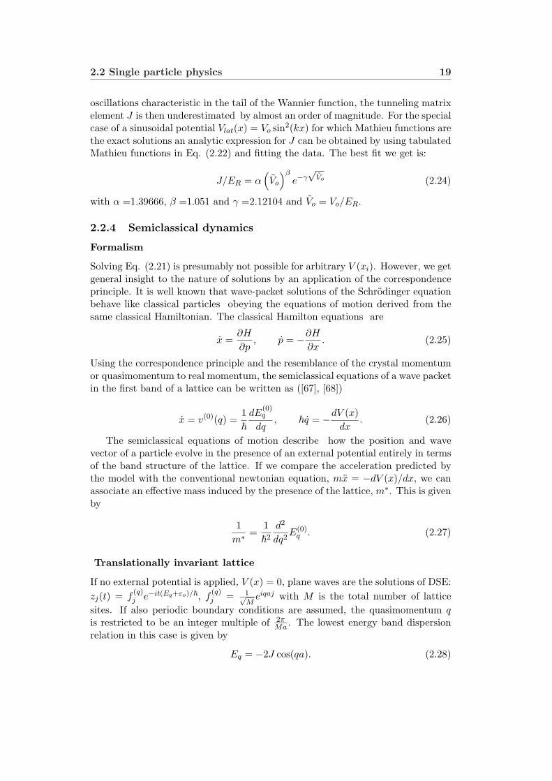
2.2 Single particle physics 19
oscillations characteristic in the tail of the Wannier function, the tunneling matrixelement J is then underestimated by almost an order of magnitude. For the specialcase of a sinusoidal potential Vlat(x) = Vo sin2(kx) for which Mathieu functions arethe exact solutions an analytic expression for J can be obtained by using tabulatedMathieu functions in Eq. (2.22) and fitting the data. The best fit we get is:
J/ER = α(Vo
)βe−γ
√Vo (2.24)
with α =1.39666, β =1.051 and γ =2.12104 and Vo = Vo/ER.
2.2.4 Semiclassical dynamics
Formalism
Solving Eq. (2.21) is presumably not possible for arbitrary V (xi). However, we getgeneral insight to the nature of solutions by an application of the correspondenceprinciple. It is well known that wave-packet solutions of the Schrodinger equationbehave like classical particles obeying the equations of motion derived from thesame classical Hamiltonian. The classical Hamilton equations are
x =∂H
∂p, p = −∂H
∂x. (2.25)
Using the correspondence principle and the resemblance of the crystal momentumor quasimomentum to real momentum, the semiclassical equations of a wave packetin the first band of a lattice can be written as ([67], [68])
x = v(0)(q) =1~
dE(0)q
dq, ~q = −dV (x)
dx. (2.26)
The semiclassical equations of motion describe how the position and wavevector of a particle evolve in the presence of an external potential entirely in termsof the band structure of the lattice. If we compare the acceleration predicted bythe model with the conventional newtonian equation, mx = −dV (x)/dx, we canassociate an effective mass induced by the presence of the lattice, m∗. This is givenby
1m∗ =
1~2
d2
dq2E(0)
q . (2.27)
Translationally invariant lattice
If no external potential is applied, V (x) = 0, plane waves are the solutions of DSE:zj(t) = f
(q)j e−it(Eq+εo)/~, f
(q)j = 1√
Meiqaj with M is the total number of lattice
sites. If also periodic boundary conditions are assumed, the quasimomentum qis restricted to be an integer multiple of 2π
Ma . The lowest energy band dispersionrelation in this case is given by
Eq = −2J cos(qa). (2.28)
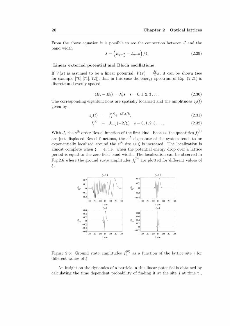
20 Chapter 2 Optical lattices
From the above equation it is possible to see the connection between J and theband width
J =(Eq=π
a−Eq=0
)/4. (2.29)
Linear external potential and Bloch oscillations
If V (x) is assumed to be a linear potential, V (x) = Jξa x, it can be shown (see
for example [70],[71],[72]), that in this case the energy spectrum of Eq. (2.21) isdiscrete and evenly spaced
(Es −E0) = Jξs s = 0, 1, 2, 3 . . . . (2.30)
The corresponding eigenfunctions are spatially localized and the amplitudes zj(t)given by :
zj(t) = f(s)j e−iEst/~, (2.31)
f(s)j = Js−j(−2/ξ) s = 0, 1, 2, 3, . . . . (2.32)
With Js the sth order Bessel function of the first kind. Because the quantities f(s)j
are just displaced Bessel functions, the sth eigenstate of the system tends to beexponentially localized around the sth site as ξ is increased. The localization isalmost complete when ξ = 4, i.e. when the potential energy drop over a latticeperiod is equal to the zero field band width. The localization can be observed inFig.2.6 where the ground state amplitudes f
(0)i are plotted for different values of
ξ.
-30 -20 -10 0 10 20 30i site
-0.6-0.4-0.2
00.20.40.6
f iH0L
Ξ=1
-30 -20 -10 0 10 20 30i site
-0.20
0.20.40.60.8
f iH0L
Ξ=4
-30 -20 -10 0 10 20 30i site
-0.2
-0.1
0
0.1
0.2
f iH0L
Ξ=0.1
-30 -20 -10 0 10 20 30i site
-0.4
-0.2
0
0.2
0.4
f iH0L
Ξ=0.5
Figure 2.6: Ground state amplitudes f(0)i as a function of the lattice site i for
different values of ξ
An insight on the dynamics of a particle in this linear potential is obtained bycalculating the time dependent probability of finding it at the site j at time t ,
2.2 Single particle physics 21
|zj(t)|2, if it was in the state localized at the origin at time zero zj(0) = δ0j . Aftersome algebra it can be shown to be given by
Pj = |zj(t)|2 = J2j
(4 sin(ξτ/2)
ξ
), (2.33)
with τ = tJ/~. The dynamical evolution of Pj 6=0, for a given j consists of an initialperiod of growth until a maximum is reached followed by an oscillatory decay. Thesequence is repeated again backwards until a time τ= 2π/ξ at which Pj 6=0 vanishesand a new cycle starts.
In Fig. 2.7, the diffusion of a square wave packet occupying at t = 0 the central20 sites is plotted. It can be seen that the center of mass of the wave functionaccelerates and then returns to its initial position after a period τ= 2π/ξ.
-40 -20 0 20 40i site
ÈΨiÈ
2
ΤH2ΠΞL=0.8
-40 -20 0 20 40i site
ÈΨiÈ
2
ΤH2ΠΞL=1.
-40 -20 0 20 40i site
ÈΨiÈ
2
ΤH2ΠΞL=0.4
-40 -20 0 20 40i site
ÈΨiÈ
2
ΤH2ΠΞL=0.6
-40 -20 0 20 40i site
ÈΨiÈ
2
ΤH2ΠΞL=0.
-40 -20 0 20 40i site
ÈΨiÈ
2
ΤH2ΠΞL=0.2
Figure 2.7: Diffusion of a square wave packet in the presence of a linear poten-tial.The parameters for the plot are ξ = 0.1.
A simplified picture of the dynamics of a wave packet in this linear potential canalso be obtained if we use the semiclassical model. If we assume a packet initiallycentered at x(t = 0) = 0, with average initial quasimomentum q(t = 0) = qo,the semiclassical model predicts periodic oscillations of the center of mass withfrequency ξ and amplitude 2/ξ.
x(t) =2ξ(1− cos(ξτ + qoa)). (2.34)
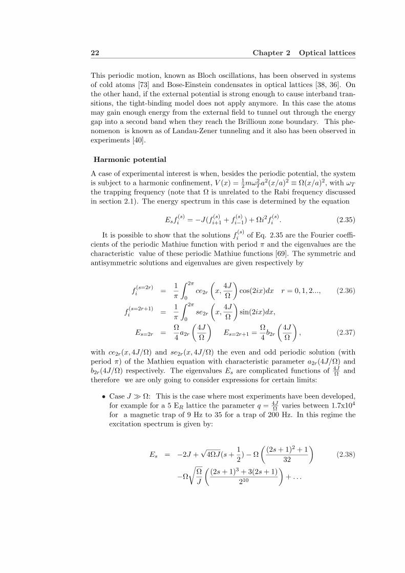
22 Chapter 2 Optical lattices
This periodic motion, known as Bloch oscillations, has been observed in systemsof cold atoms [73] and Bose-Einstein condensates in optical lattices [38, 36]. Onthe other hand, if the external potential is strong enough to cause interband tran-sitions, the tight-binding model does not apply anymore. In this case the atomsmay gain enough energy from the external field to tunnel out through the energygap into a second band when they reach the Brillioun zone boundary. This phe-nomenon is known as of Landau-Zener tunneling and it also has been observed inexperiments [40].
Harmonic potential
A case of experimental interest is when, besides the periodic potential, the systemis subject to a harmonic confinement, V (x) = 1
2mω2T a2(x/a)2 ≡ Ω(x/a)2, with ωT
the trapping frequency (note that Ω is unrelated to the Rabi frequency discussedin section 2.1). The energy spectrum in this case is determined by the equation
Esf(s)i = −J(f (s)
i+1 + f(s)i−1) + Ωi2f
(s)i . (2.35)
It is possible to show that the solutions f(s)i of Eq. 2.35 are the Fourier coeffi-
cients of the periodic Mathiue function with period π and the eigenvalues are thecharacteristic value of these periodic Mathiue functions [69]. The symmetric andantisymmetric solutions and eigenvalues are given respectively by
f(s=2r)i =
1π
∫ 2π
0ce2r
(x,
4J
Ω
)cos(2ix)dx r = 0, 1, 2..., (2.36)
f(s=2r+1)i =
1π
∫ 2π
0se2r
(x,
4J
Ω
)sin(2ix)dx,
Es=2r =Ω4
a2r
(4J
Ω
)Es=2r+1 =
Ω4
b2r
(4J
Ω
), (2.37)
with ce2r(x, 4J/Ω) and se2r(x, 4J/Ω) the even and odd periodic solution (withperiod π) of the Mathieu equation with characteristic parameter a2r(4J/Ω) andb2r(4J/Ω) respectively. The eigenvalues Es are complicated functions of 4J
Ω andtherefore we are only going to consider expressions for certain limits:
• Case J À Ω: This is the case where most experiments have been developed,for example for a 5 ER lattice the parameter q = 4J
Ω varies between 1.7x10⁴
for a magnetic trap of 9 Hz to 35 for a trap of 200 Hz. In this regime theexcitation spectrum is given by:
Es = −2J +√
4ΩJ(s +12)− Ω
((2s + 1)2 + 1
32
)(2.38)
−Ω
√ΩJ
((2s + 1)3 + 3(2s + 1)
210
)+ . . .

2.2 Single particle physics 23
which to a first approximation is just the harmonic potential found if nolattice were present but with an effective frequency ω∗ and effective mass m∗
given by
~ω∗ =√
4ΩJ = ~ωt
√m
m∗ , (2.39)
m∗ =~2
2Ja2, (2.40)
It is worth it to emphasize that this result was derived under the tight-binding approximation and therefore it is not valid for very shallow lattices.The harmonic character of the spectrum can be easily checked if we take thecontinuous limit of Eq. (2.35). The differential equation obtained is just theharmonic oscillator equation,
(Es + 2J)f (s)(x) = − ~2
2m∗∂f (s)(x)
∂x2+
12m∗ω∗2x2f (s)(x). (2.41)
The average width of the wave function is just aho=√
m∗ω∗ .
• Case J ¿ Ω: The single particle spectrum in this case is given by
Es=2n ≈ Es=2n−1
=Ω4
((2n)2 +
(4J
Ω
)2 1((2n)2 − 1)
+ O
(4J
Ω
)4
+ ..
)n ≥ 3,
E4 ≈ E3 =Ω4
(16 +
(4J
Ω
)2 130
+ ..
),
E2 =Ω4
(4 +
(4J
Ω
)2 512
+ ..
), (2.42)
E1 =Ω4
(4−
(4J
Ω
)2 112
+ ..
),
E0 =Ω4
(−
(4J
Ω
)2 12
+ ...
).
It can be appreciated that the spectrum is nearly twofold degenerate and it goeslike Ωn2 to first order in (J/Ω) . In this regime then, the trapping potential iswhat mostly determines the energy spacing. In Fig. 2.8 the spectrum is shown fordifferent values of 4J
Ω .

24 Chapter 2 Optical lattices
5 10 15 20nth
4
162
321
En
J
4JW=1
5 10 15 20nth
40
1624
3208
En
J
4JW=0.1
5 10 15 20nth
2
4
En
J
4JW=100
5 10 15 20nth
1
17
33
En
J
4JW=10
Figure 2.8: Harmonic confinement plus lattice spectrum: The index n labels theeigenvalues in increasing energy order.

Chapter 3
The Bose-HubbardHamiltonian and the superfluidto Mott insulator transition
In chapter 2 we studied the physics of non interacting particles in a periodic system.In this chapter we go one step ahead and describe the basic properties of a bosonicmany body system with repulsive interactions in a periodic lattice potential.
The simplest non trivial model that describes interacting bosons in a periodicpotential is the Bose Hubbard Hamiltonian. It includes the main physics thatdescribe strongly interacting bosons, which is the competition between kinetic andinteraction energy. This model has been used to describe many different systemsin solid state physics, like short correlation length superconductors, Josephson ar-rays, critical behavior of 4 He and, recently, cold atoms in optical lattices [43]. Ithas been studied analytically with many different techniques such as mean fieldapproximations [74, 75, 77], renormalization group theories [44] and strong cou-pling expansions [78]. Numerically most of the studies are based on quantumMonte Carlo methods and density matrix renormalization techniques [79]. TheBose Hubbard Hamiltonian predicts a quantum phase transition from a superfluidto a Mott insulator state. This transition has been observed experimentally inatoms confined in a 3D optical lattice [46]. In this chapter we start by review-ing the basic properties of the Bose Hubbard Hamiltonian and outline the mostimportant aspects that characterize the superfluid to Mott insulator transition.
3.1 Bose-Hubbard Hamiltonian
We begin the analysis by considering the second quantized Hamiltonian that de-scribes interacting bosonic atoms in an external trapping potential plus lattice. Inthe grand canonical ensemble it is given by:

26Chapter 3 The Bose-Hubbard Hamiltonian and the superfluid to
Mott insulator transition
H =∫
dxΦ†(x)(− ~
2
2m∇2 + Vlat(x)
)Φ(x) + (V (x)− µ)Φ†(x)Φ(x) (3.1)
+12
∫dxdx′Φ†(x)Φ†(x′)Vat(x− x′)Φ(x)Φ(x′),
where Φ†(x) is the bosonic field operator which creates an atom at the positionx, Vlat(x) is the periodic lattice potential, V (x) denotes any additional slowly-varying external potential that might be present (such as a magnetic trap), µ isthe chemical potential and acts as a lagrange multiplier to fix the mean numberof atoms in the grand canonical ensemble and Vat(x) is the interatomic scatteringpotential, which is in general a complicated function. However, since for cold gasesthe thermal de Broglie wavelength is much larger than the effective extension of theinteraction potential, the only relevant scattering process is the s-wave scattering,and the actual inter-particle potential plays a minor role. Therefore, to a goodapproximation, the interatomic potential can be replaced by an effective contactinteraction:
Vat(x) ≈ 4πas~2
mδ(x), (3.2)
with as is the scattering length and m the mass of an atom. In this thesis weare going to assume that the scattering length is positive so the interactions arerepulsive.
Similar to the noninteracting situation, where we used Wannier orbitals to ex-pand the single particle wave function, it is convenient to expand the field operatorin a Wannier orbital basis. If the chemical potential of the system is less than thesingle particle excitation energy to the second band, only the first band has to beconsidered and the field operator can be written as:
Φ(x) =∑
n
anw0(x− xn), (3.3)
where w0(x) is the Wannier orbital of the lowest vibrational band localized at theorigin, and an is the annihilation operator at site n which obeys bosonic canonicalcommutation relations. The sum is taken over the total number of lattice sites.If Eq. (3.3) is inserted in H and only tunneling between nearest neighbors isconsidered, we obtain the Bose Hubbard Hamiltonian
HBH = −J∑
<n,m>
a†nam +12U
∑n
a†na†nanan +∑
n
(Vn − µ)a†nan, (3.4)
with
3.2 Superfluid-Mott insulator transition 27
J = −∫
dxw∗0(x− xn)(
p2
2m+ Vlat(x)
)w0(x + xn+1), (3.5)
U =4πas~2
m
∫dx |w0(x)|4 , (3.6)
Vn = V (xn). (3.7)
The first term in the Hamiltonian proportional to J is a measure of the kineticenergy of the system. J is the hopping matrix element between nearest neighbors(see also 2.24). Here the notation < n,m > restricts the sum to nearest-neighborssites. Next-to-nearest neighbor tunneling amplitudes are typically two orders ofmagnitude smaller than nearest-neighbor tunneling amplitudes, and to a goodapproximation they can be neglected.
The second term determines the interaction energy of the system. The param-eter U measures the strength of the repulsion of two atoms at lattice site n.Theintegral (3.6) is not as sensitive as Eq. (3.5) to the oscillatory tails characteristicof the Wannier orbitals, and a Gaussian approximation can be used to estimateit [43]. Under the Gaussian approximation, the ground state wave function cen-tered at the origin of a separable sinusoidal lattice, with lattice depth Vj0 in the
jth direction, has the form w0(0) ∼ ∏j exp−
(xj√2ahoj
)2, with ahoj =
√~
mωhojand
ωhoj =√
4ErVj0
~2 . Using this ansatz in the integral (3.6) yields an onsite interactiongiven by
U =~as√2π
ωho
aho, (3.8)
with the bar indicating the geometric mean. To guarantee the validity of the oneband approximation, the mean interaction energy per particle UN must be smallerthan the energy gap to the first vibrational excitation, i.e. UN < ~ωho. N is themean number of atoms. This inequality is readily satisfied in practice.
The third term in the Hamiltonian takes into account the energy offset at siten due to a slowly varying external potential V (x).
The realization of the Bose-Hubbard Hamiltonian using optical lattices has theadvantage that the interaction matrix element U and the tunneling matrix elementJ can be controlled by adjusting the intensity of the laser beams. As the intensityof the lattice is increased the tunneling rate decreases exponentially and the onsideinteraction increases as a power law, V
d/40 , (d is the dimensionality of the lattice).
3.2 Superfluid-Mott insulator transition
At zero temperature the physics described by the Bose-Hubbard Hamiltonian canbe divided into two different regimes. One is the interaction dominated regime
28Chapter 3 The Bose-Hubbard Hamiltonian and the superfluid to
Mott insulator transition
when J is much smaller than U , and the system is in the Mott insulator phase.The other is the kinetic energy dominated regime, where tunneling overwhelms therepulsion and the system exhibits superfluid properties. The onset of superfluidityis a consequence of the competition between the kinetic energy, which tries todelocalize the particles, and the interaction energy, which tries to localize themand make the number fluctuations small.
In the superfluid regime, the kinetic energy term dominates the Hamiltonian.In this regime, quantum correlations can be neglected and the system can bedescribed by a macroscopic wave function since the many body state is almosta product over identical single particle wave functions. There is a macroscopicwell-defined phase and the system is a superfluid. Because atoms are delocalizedover the lattice with equal relative phases between adjacent sites, they exhibit aninterference pattern when the lattice is turned off, as expected from an array ofphase coherent matter wave sources. As interaction increases the average kineticenergy required for an atom to hop from one site to the next becomes insufficientto overcome the potential energy cost. Atoms tend to get localized at individuallattice sites and number fluctuations are reduced. In the Mott insulator phasethe ground state of the system instead consists of localized atomic wave functionswith a fixed number of atoms per site. The lowest lying excitations that conserveparticle number are particle-hole excitations (adding plus removing a particle fromthe system). This phase is characterized by the existence of an energy gap. Thegap is determined by the energy necessary to create one particle-hole pair.
The phase diagram [44],[74]-[76] that describes the Mott insulator transitionof a translational invariant system with Vn = 0 exhibits lobe-like Mott insulatingphases in the J-µ plane, see Fig. 3.1. Each Mott lobe is characterized by havinga fixed integer density. Inside these lobes the compressibility, ∂ρ/∂µ with ρ theaverage density of the system, vanishes. The physics behind this diagram can beunderstood as follows: If we start at some point in the Mott insulating phase andincrease µ keeping J fixed, there is going to be a point at which the kinetic energyof adding an extra particle and letting it hop around will balance the interactionenergy cost. With an extra particle free to move around the lattice phase coherenceis recovered and the system enters the superfluid regime. Similarly, by decreasingµ from a point in the Mott phase, at some point eventually it will be energeticallyfavorable to remove one particle from the system. The extra mobile hole will inducealso phase coherence and the system will condense in a superfluid state. Since thekinetic energy of the system increases with J the width of the lobes decreases withJ . The distance in the µ direction at fixed J between the upper and lower part ofthe lobe is the energy gap. At J = 0 the gap is just equal to U . Also at J = 0 theintersection points between the lobes with density ρ = n and the ones with densityρ = n + 1 are degenerate. Because there is no energy barrier to the addition ofan extra particle at these degenerated points the system remain superfluid. Mottinsulator phases occur only at integer densities; non-integer density contours lieentirely in the superfluid phase because there is always an extra particle that canhop without energy cost.
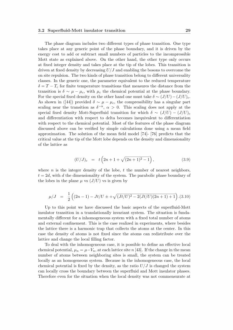
3.2 Superfluid-Mott insulator transition 29
The phase diagram includes two different types of phase transition. One typetakes place at any generic point of the phase boundary, and it is driven by theenergy cost to add or subtract small numbers of particles to the incompressibleMott state as explained above. On the other hand, the other type only occursat fixed integer density and takes place at the tip of the lobes. This transition isdriven at fixed density by decreasing U/J and enabling the bosons to overcome theon site repulsion. The two kinds of phase transition belong to different universalityclasses. In the generic one, the parameter equivalent to the reduced temperatureδ = T − Tc for finite temperature transitions that measures the distance from thetransition is δ ∼ µ − µc, with µc the chemical potential at the phase boundary.For the special fixed density on the other hand one must take δ ∼ (J/U)− (J/U)c.As shown in ([44]) provided δ ∼ µ − µc, the compressibility has a singular partscaling near the transition as δ−α, α > 0. This scaling does not apply at thespecial fixed density Mott-Superfluid transition for which δ ∼ (J/U) − (J/U)c
and differentiation with respect to delta becomes inequivalent to differentiationwith respect to the chemical potential. Most of the features of the phase diagramdiscussed above can be verified by simple calculations done using a mean fieldapproximation. The solution of the mean field model [74]- [76] predicts that thecritical value at the tip of the Mott lobe depends on the density and dimensionalityof the lattice as
(U/J)c = t(2n + 1 +
√(2n + 1)2 − 1
), (3.9)
where n is the integer density of the lobe, t the number of nearest neighbors,t = 2d, with d the dimensionality of the system. The parabolic phase boundary ofthe lobes in the plane µ vs (J/U) vs is given by
µ/J =12
((2n− 1)− Jt/U ±+
√(Jt/U)2 − 2(Jt/U)(2n + 1) + 1
).(3.10)
Up to this point we have discussed the basic aspects of the superfluid-Mottinsulator transition in a translationally invariant system. The situation is funda-mentally different for a inhomogeneous system with a fixed total number of atomsand external confinement. This is the case realized in experiments, where besidesthe lattice there is a harmonic trap that collects the atoms at the center. In thiscase the density of atoms is not fixed since the atoms can redistribute over thelattice and change the local filling factor.
To deal with the inhomogeneous case, it is possible to define an effective localchemical potential, µn = µ−Vn, at each lattice site n [43]. If the change in the meannumber of atoms between neighboring sites is small, the system can be treatedlocally as an homogeneous system. Because in the inhomogeneous case, the localchemical potential is fixed by the density, as the ratio U/J is changed the systemcan locally cross the boundary between the superfluid and Mott insulator phases.Therefore even for the situation when the local density was not commensurate at
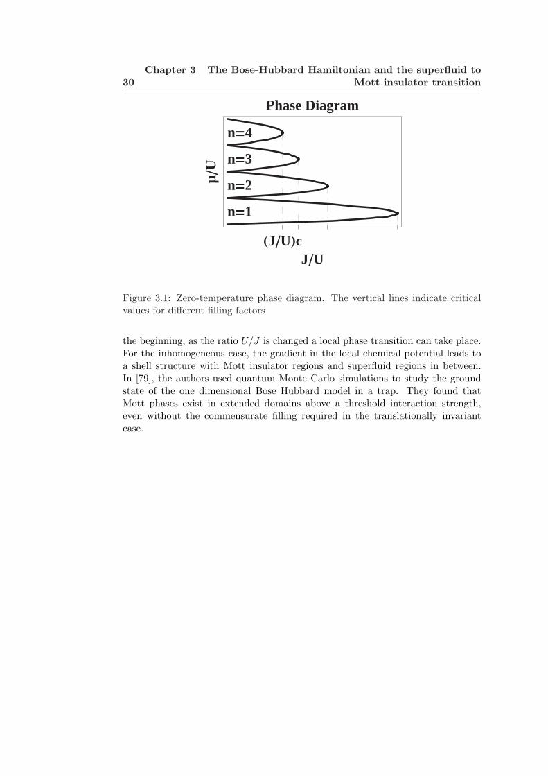
30Chapter 3 The Bose-Hubbard Hamiltonian and the superfluid to
Mott insulator transition
HJULcJU
µU
Phase Diagram
n=1
n=2
n=3
n=4
Figure 3.1: Zero-temperature phase diagram. The vertical lines indicate criticalvalues for different filling factors
the beginning, as the ratio U/J is changed a local phase transition can take place.For the inhomogeneous case, the gradient in the local chemical potential leads toa shell structure with Mott insulator regions and superfluid regions in between.In [79], the authors used quantum Monte Carlo simulations to study the groundstate of the one dimensional Bose Hubbard model in a trap. They found thatMott phases exist in extended domains above a threshold interaction strength,even without the commensurate filling required in the translationally invariantcase.
Chapter 4
Mean field theory
In this chapter we introduce the mean field Discrete Nonlinear Schrodinger equa-tions and use it first to investigate the behavior of a BEC adiabatically loaded intoan optical lattice moving at constant velocity, and second to model the dynamicalevolution of a BEC initially loaded into every third site of an optical lattice.
4.1 Discrete nonlinear Schrodinger equation (DNLSE)
In the weakly interacting regime, quantum fluctuations can be neglected to a goodapproximation. In this regime most of the atoms occupy the same condensatewave function. The macroscopic occupation of a single mode implies that thecommutator of the annihilation and creation operators that create and destroy aparticle in the condensate mode can be neglected with respect to the total numberof atoms in the mode. Therefore, to a good approximation the field operator canbe replaced by a c-number,
Φ(x) → ϕ(x). (4.1)
This procedure can be interpreted as giving to the field operator a non zero average,〈Φ(x)〉 = ϕ(x), and thus a well defined phase to system. Because the originalHamiltonian is invariant under global phase transformation, this definition of BECcorresponds to an spontaneous symmetry breaking [11, 12, 80]. The function ϕ(x)is a classical field having the meaning of an order parameter and is often calledthe ”condensate wave function”. It characterizes the off-diagonal long range orderpresent in the one particle density matrix [81].
lim|x′−x|→∞
〈Φ†(x′)Φ(x)〉 = ϕ∗(x′)ϕ(x). (4.2)
Strictly speaking, neither the concept of broken symmetry, nor the one of off-diagonal long range order can be applied to finite size systems with well definednumber of particles. However the condensate wave function can still be determinedby diagonalization of the one particle density matrix. The eigenstate with largereigenvalue corresponds to ϕ(x).
32 Chapter 4 Mean field theory
If we use the approximation (4.1) in the many-body Hamiltonian (3.1) we geta classical Hamiltonian given by:
H =∫
dxϕ†(x)(− ~
2
2m∇2 + Vlat(x)
)ϕ(x) + (V (x)− µ)ϕ†(x)ϕ(x) (4.3)
+12
4πas~2
m
∫dxϕ†(x)ϕ†(x)ϕ(x)ϕ(x),
The time dependent equations of motion for the condensate wave function can beobtained from the variational principle by minimizing the quantity i~ ∂
∂t − H. Theminimization yields
i~∂ϕ(x)
∂t=
(− ~
2
2m∇2 + Vlat(x) + V (x) +
4πas~2
m|ϕ(x)|2
)ϕ(x) (4.4)
This equation is known as the Gross-Pitaevskii equation (GPE). It was derived byindependently by Gross and Pitaevskii [10].
If the chemical potential is small compared to the vibrational level spacingand the lattice depth is deep enough that a tight binding picture is valid, thecondensate order parameter can be expanded in a Wannier basis keeping only thelowest band orbitals:
ϕ(x, t) =∑
n
zn(t)w0(x− xn). (4.5)
Using this ansatz in Eq. (4.4), the Gross-Pitaevskii equation reduces to thediscrete nonlinear Schroedinger equation (DNLSE), where the zn amplitudes sat-isfy:
i~∂zn
∂t= −J
∑<n,m>
zm + (Vn + UN |zn|2)zn, (4.6)
where < n,m > restricts the sum over nearest neighbors, the parameters J and Uare the ones defined in Eq. (3.5) and (3.6) and N is the total number of particles.The normalization condition for the amplitudes is given by:
∑n
|zn|2 = 1. (4.7)
Notice the DNLSE can also be derived by assuming the field operators present inthe Bose-Hubbard Hamiltonian to be c-numbers,i.e. an = zn(t). This assumptionleads to a tight-binding classical Hamiltonian, which can be minimized using thevariational principle.
H = −J∑
<n,m>
z∗nzm +∑
n
(Vn|zn|2 +
U
2|zn|4
). (4.8)
4.2 Dragging experiment 33
The DNLSE is similar to its linear counterpart, the DSE or tight-bindingSchrodinger equation (see 2.21), but with an extra cubic term, which takes intoaccount mean field interaction effects. To see the modification that the nonlinearterm introduces in the dispersion relation, we consider a one dimensional opticallattice with M sites and periodic boundary conditions.
In the translational invariant case with no other external potential present,Vn = 0, the solutions of the DNLSE that are similar to those of the noninteractingcase are, zn =
√no exp(−inq) exp (−iEqt/~), with no = N/M the condensate
density. Using this plane wave ansatz in the DNLSE we get a dispersion relationgiven by:
Eq = −2J cos(qa) + Uno (4.9)
In the tight-binding approximation, mean field interactions do not modify theshape of the lowest band: it has still a cosine dependence with bandwith equal to4J . The only difference with respect to the single particle case is an energy shiftin the dispersion relation which takes into account the average mean field energyUno.
It is important to mention though, that outside the range of validity of atight-binding model, nonlinear effects does not necessarily change the dispersionrelation in a simple way, especially at the edge of the Brillouin zone. It has beenshown in the literature [82, 83] that if the chemical potential is bigger than thegap vibrational excitation energy to higher bands, the lowest band becomes triplevalued near the Brilloiun zone edge and a loop appears at this point. This loopreflects the existence of new solutions, which only exist when the tight-bindingapproximation is not valid. These new solutions have a non zero velocity at theedge of the Brillouin zone, as opposed to the linear case. The nonzero velocitycarried by the Bloch waves is a manifestation of the superfluidity of the system.For free particles the flow is stopped completely by Bragg scattering from theperiodic potential, but if interactions are strong enough the superfluid flow can nolonger be stopped.
4.2 Dragging experiment
In this section we investigate an experiment done at NIST where a Bose-Einsteincondensate was prepared in a harmonic trap and adiabatically loaded into a onedimensional optical lattice moving at constant velocity Ref. [37]. We first study thedynamics in a translationally invariant lattice using a simple single particle picture,and show how the center-of-mass motion of the condensate can be used as a probeof the lattice band structure. Then we discuss the effects of the trapping potentialand interaction effects on the dynamics. When mean field effects are included,they cause the effective mass of the Bloch state to depend on time, influencingthe condensate dynamics in the lattice. As a consequence, characteristic nonlineareffects such as solitons, self focusing effects and dynamical stabilities might beobserved.

34 Chapter 4 Mean field theory
4.2.1 Experiment
In the experiment, a condensate prepared in the ground state of a harmonic trapis loaded in an optical lattice, which is moved at constant velocity. The loadingof the condensate in the optical lattice is done by turning on the lattice, linearlyin time, up to some maximum height. The important part of this turning on isthat it is done sufficiently slow to be adiabatic with respect to band excitations.After the maximum is reached, at t = tr, the lattice depth is held constant for afixed period of time and the system is allowed to expand in the lattice. Finally att = tf the condensate density distribution along the lattice axis is imaged. Thetemporal dependence of the optical lattice depth is shown in Fig. 4.1. In the figure,experimental results obtained for the final condensate density for different latticedepths are also shown. The general observation is that the deeper the lattice, thegreater the response of the condensate to the lattice motion. In this experiment,the condensate has a very narrow momentum spread compared to the lattice recoilmomentum.
Figure 4.1: Condensate density in the x-direction at the observation time tf . Lightcolors areas indicate regions of high condensate density. The dashed line indicatesthe final location of a co-moving point with the optical lattice.
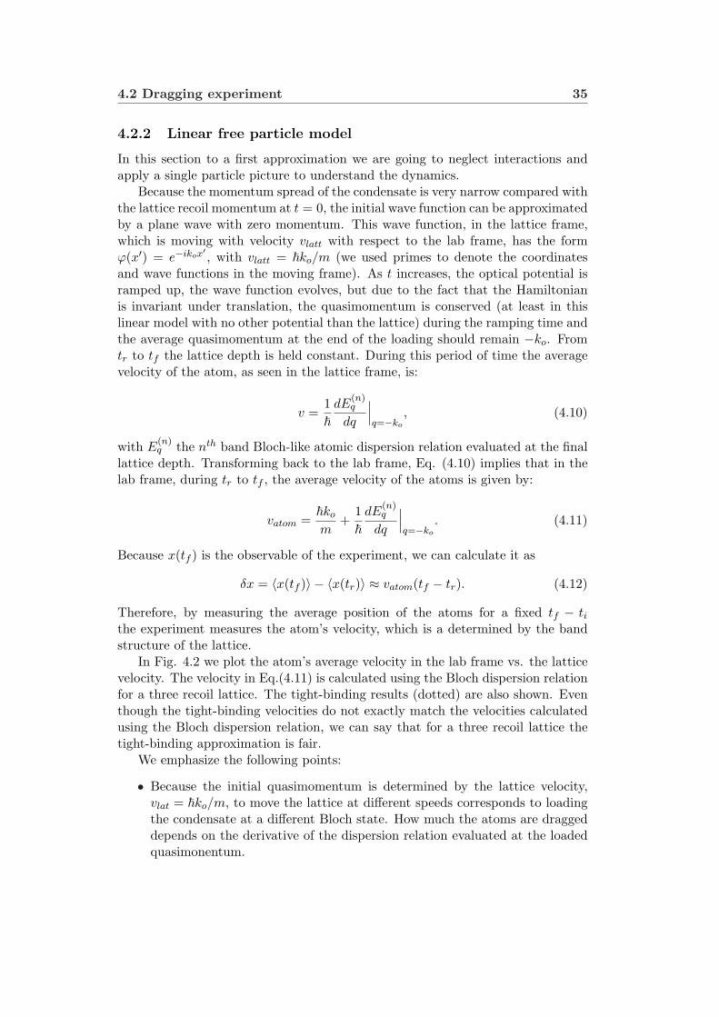
4.2 Dragging experiment 35
4.2.2 Linear free particle model
In this section to a first approximation we are going to neglect interactions andapply a single particle picture to understand the dynamics.
Because the momentum spread of the condensate is very narrow compared withthe lattice recoil momentum at t = 0, the initial wave function can be approximatedby a plane wave with zero momentum. This wave function, in the lattice frame,which is moving with velocity vlatt with respect to the lab frame, has the formϕ(x′) = e−ikox′ , with vlatt = ~ko/m (we used primes to denote the coordinatesand wave functions in the moving frame). As t increases, the optical potential isramped up, the wave function evolves, but due to the fact that the Hamiltonianis invariant under translation, the quasimomentum is conserved (at least in thislinear model with no other potential than the lattice) during the ramping time andthe average quasimomentum at the end of the loading should remain −ko. Fromtr to tf the lattice depth is held constant. During this period of time the averagevelocity of the atom, as seen in the lattice frame, is:
v =1~
dE(n)q
dq
∣∣∣q=−ko
, (4.10)
with E(n)q the nth band Bloch-like atomic dispersion relation evaluated at the final
lattice depth. Transforming back to the lab frame, Eq. (4.10) implies that in thelab frame, during tr to tf , the average velocity of the atoms is given by:
vatom =~ko
m+
1~
dE(n)q
dq
∣∣∣q=−ko
. (4.11)
Because x(tf ) is the observable of the experiment, we can calculate it as
δx = 〈x(tf )〉 − 〈x(tr)〉 ≈ vatom(tf − tr). (4.12)
Therefore, by measuring the average position of the atoms for a fixed tf − tithe experiment measures the atom’s velocity, which is a determined by the bandstructure of the lattice.
In Fig. 4.2 we plot the atom’s average velocity in the lab frame vs. the latticevelocity. The velocity in Eq.(4.11) is calculated using the Bloch dispersion relationfor a three recoil lattice. The tight-binding results (dotted) are also shown. Eventhough the tight-binding velocities do not exactly match the velocities calculatedusing the Bloch dispersion relation, we can say that for a three recoil lattice thetight-binding approximation is fair.
We emphasize the following points:
• Because the initial quasimomentum is determined by the lattice velocity,vlat = ~ko/m, to move the lattice at different speeds corresponds to loadingthe condensate at a different Bloch state. How much the atoms are draggeddepends on the derivative of the dispersion relation evaluated at the loadedquasimonentum.
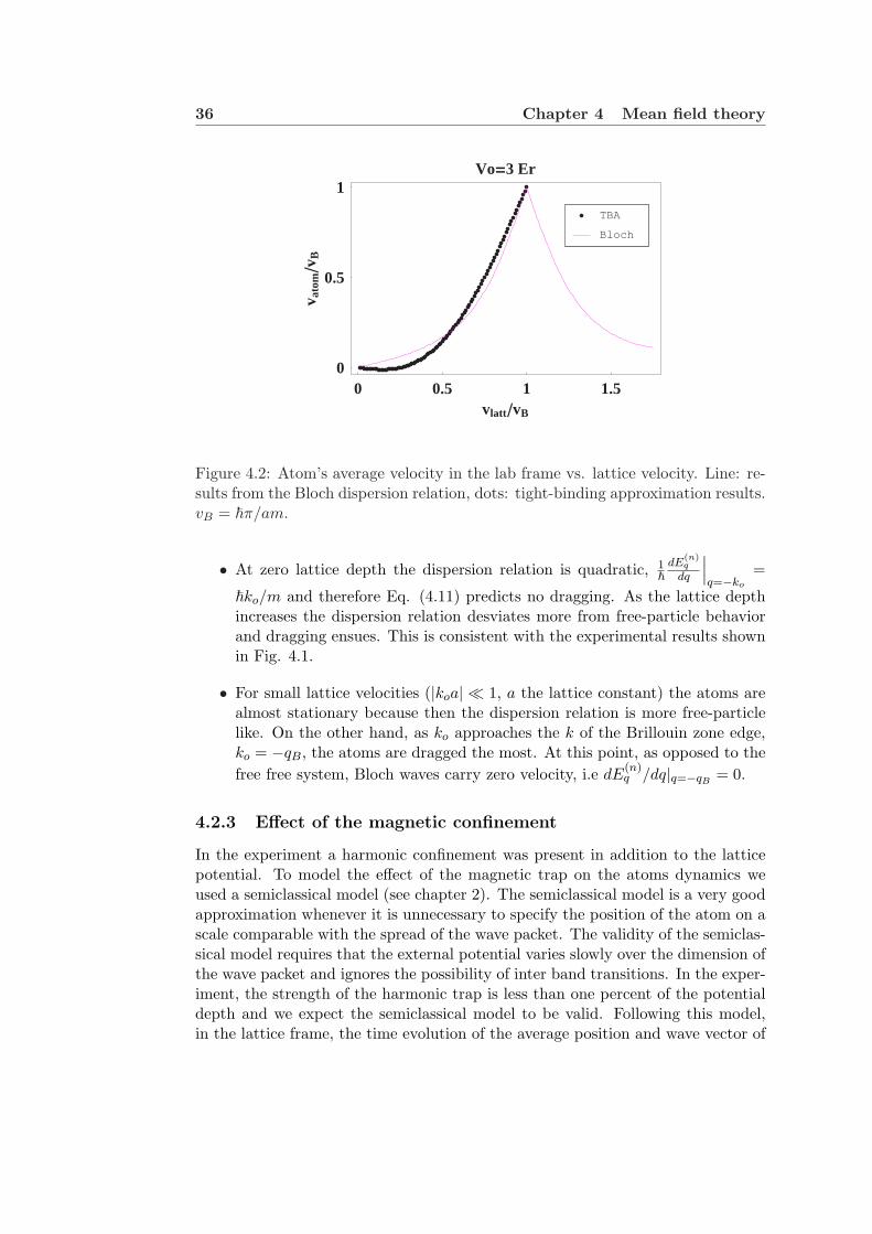
36 Chapter 4 Mean field theory
0 0.5 1 1.5vlattvB
0
0.5
1
v ato
mv
B
Vo=3 Er
Bloch
TBA
Figure 4.2: Atom’s average velocity in the lab frame vs. lattice velocity. Line: re-sults from the Bloch dispersion relation, dots: tight-binding approximation results.vB = ~π/am.
• At zero lattice depth the dispersion relation is quadratic, 1~
dE(n)q
dq
∣∣∣q=−ko
=
~ko/m and therefore Eq. (4.11) predicts no dragging. As the lattice depthincreases the dispersion relation desviates more from free-particle behaviorand dragging ensues. This is consistent with the experimental results shownin Fig. 4.1.
• For small lattice velocities (|koa| ¿ 1, a the lattice constant) the atoms arealmost stationary because then the dispersion relation is more free-particlelike. On the other hand, as ko approaches the k of the Brillouin zone edge,ko = −qB, the atoms are dragged the most. At this point, as opposed to thefree free system, Bloch waves carry zero velocity, i.e dE
(n)q /dq|q=−qB = 0.
4.2.3 Effect of the magnetic confinement
In the experiment a harmonic confinement was present in addition to the latticepotential. To model the effect of the magnetic trap on the atoms dynamics weused a semiclassical model (see chapter 2). The semiclassical model is a very goodapproximation whenever it is unnecessary to specify the position of the atom on ascale comparable with the spread of the wave packet. The validity of the semiclas-sical model requires that the external potential varies slowly over the dimension ofthe wave packet and ignores the possibility of inter band transitions. In the exper-iment, the strength of the harmonic trap is less than one percent of the potentialdepth and we expect the semiclassical model to be valid. Following this model,in the lattice frame, the time evolution of the average position and wave vector of
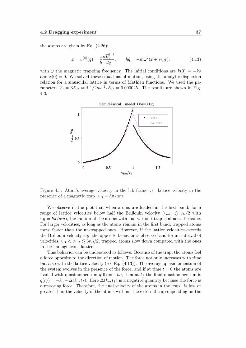
4.2 Dragging experiment 37
the atoms are given by Eq. (2.26):
x = v(n)(q) =1~
dE(n)q
dq, ~q = −mω2(x + vlatt), (4.13)
with ω the magnetic trapping frequency. The initial conditions are k(0) = −koand x(0) = 0. We solved these equations of motion, using the analytic dispersionrelation for a sinusoidal lattice in terms of Mathieu functions. We used the pa-rameters V0 = 3ER and 1/2mω2/ER = 0.000025. The results are shown in Fig.4.3.
0 0.5 1 1.5vlattvB
0
0.5
1
v ato
mv
B
Semiclassical model HVo=3 ErL
no trap
trap
Figure 4.3: Atom’s average velocity in the lab frame vs. lattice velocity in thepresence of a magnetic trap. vB = ~π/am.
We observe in the plot that when atoms are loaded in the first band, for arange of lattice velocities below half the Brillouin velocity (vlatt . vB/2 withvB = ~π/am), the motion of the atoms with and without trap is almost the same.For larger velocities, as long as the atoms remain in the first band, trapped atomsmove faster than the un-trapped ones. However, if the lattice velocities exceedsthe Brillouin velocity, vB, the opposite behavior is observed and for an interval ofvelocities, vB < vlatt . 3vB/2, trapped atoms slow down compared with the onesin the homogeneous lattice.
This behavior can be understood as follows: Because of the trap, the atoms feela force opposite to the direction of motion. The force not only increases with timebut also with the lattice velocity (see Eq. (4.13)). The average quasimomentum ofthe system evolves in the presence of the force, and if at time t = 0 the atoms areloaded with quasimomentum q(0) = −ko, then at tf the final quasimomentum isq(tf ) = −ko + ∆(ko, tf ). Here ∆(ko, tf ) is a negative quantity because the force isa restoring force. Therefore, the final velocity of the atoms in the trap , is less orgreater than the velocity of the atoms without the external trap depending on the

38 Chapter 4 Mean field theory
sign of the effective mass (sign of the curvature of the dispersion relation) evaluatedat the final momentum. If the effective mass is positive, d2Eq
dq2 > 0, (0 < q < π/2a,π/a < q < 3π/2a,...), the group velocity is an increasing function of q and thevelocity of the trapped atoms is less than the untrapped atoms’ velocity. On theother hand, when the effective mass is negative,(π/2a < q < π/a,...), the groupvelocity is a decreasing function of q and the trapped atoms speed up with respectto the untrapped ones. The more pronounced difference between trapped and un-trapped atom velocities observed in the second band with respect to the first one,is not only because ∆ increases with the lattice velocity but also because of thediscontinuous change of the band structure when crossing the Brillouin zone edge.Besides the sign difference in the curvature the second band has a larger bandwidth than the first one.
4.2.4 Interaction effects
To model the effect of the interatomic interactions on the dynamics we used thetight-binding variational method proposed in Ref. ([84, 85]). In these referencethe authors assume a Gaussian profile wave packet
zn(t) = 4
√2
γ2πe[−(n−ξ)2/γ2+ik(n−ξ)+iδ(n−ξ)2/2], (4.14)
and used ξ, γ, k, δ as variational parameters. The equations of motion they foundare:
k = −∂V
∂ξ, (4.15)
ξ = 2J sin(k)e−η, (4.16)
δ = 2J cos(k)e−η
(4γ4− δ2
)+
2NU√πγ3
− 4γ
∂V
∂γ, (4.17)
γ = 2J cos(k)e−ηγδ, (4.18)
with η =(
12γ2 − δ2γ2
8
), V =
√2/γ2π
∫dxV (x) exp[−2(x − ξ)2/γ2] and the time
scaled as t → tEr/~. Notice that the variable k is just the average quasimomentumof the wave packet. We can also associate an inverse effective mass given bym∗−1 = 2J cos(k)e−η.
We numerically integrated the equations of motion assuming no other externaltrapping potential besides the lattice, V = 0. In this case the Hamiltonian isinvariant under translations and we expect conservation of the quasimomentum.This is seen in the above equations, because if V = 0 then dk/dt = 0. Theparameters were chosen according to the experiment: γ(0) = 10, δ(0) = 0 andNU = 2ER. The bandwidth J , was found using Mathieu functions assuming a3ER lattice. We plot Fig. 4.4 vatom vs vlatt evaluated at t = 50. The curve foundis plotted in
When mean field effects are included, the dynamics of the system becomesvery rich. Depending on the the initial quasimomentum and width of the packet,
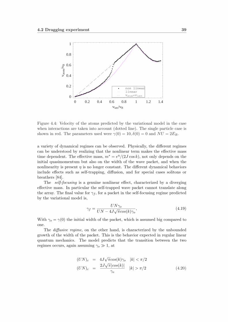
4.2 Dragging experiment 39
0 0.2 0.4 0.6 0.8 1 1.2 1.4vlattvB
0
0.2
0.4
0.6
0.8
1
v ato
mv
B
vatom=vlattlinearnon linear
Figure 4.4: Velocity of the atoms predicted by the variational model in the casewhen interactions are taken into account (dotted line). The single particle case isshown in red. The parameters used were γ(0) = 10, δ(0) = 0 and NU = 2ER.
a variety of dynamical regimes can be observed. Physically, the different regimescan be understood by realizing that the nonlinear term makes the effective masstime dependent. The effective mass, m∗ = eη/(2J cos k), not only depends on theinitial quasimomentum but also on the width of the wave packet, and when thenonlinearity is present η is no longer constant. The different dynamical behaviorsinclude effects such as self-trapping, diffusion, and for special cases solitons orbreathers [84].
The self-focusing is a genuine nonlinear effect, characterized by a divergingeffective mass. In particular the self-trapped wave packet cannot translate alongthe array. The final value for γf , for a packet in the self-focusing regime predictedby the variational model is,
γf =UNγo
UN − 4J√
πcos(k)γo, (4.19)
With γo = γ(0) the initial width of the packet, which is assumed big compared toone.
The diffusive regime, on the other hand, is characterized by the unboundedgrowth of the width of the packet. This is the behavior expected in regular linearquantum mechanics. The model predicts that the transition between the tworegimes occurs, again assuming γo À 1, at
(UN)c = 4J√
πcos(k)γo |k| < π/2
(UN)c =2J√
π|cos(k)|γo
|k| > π/2 (4.20)
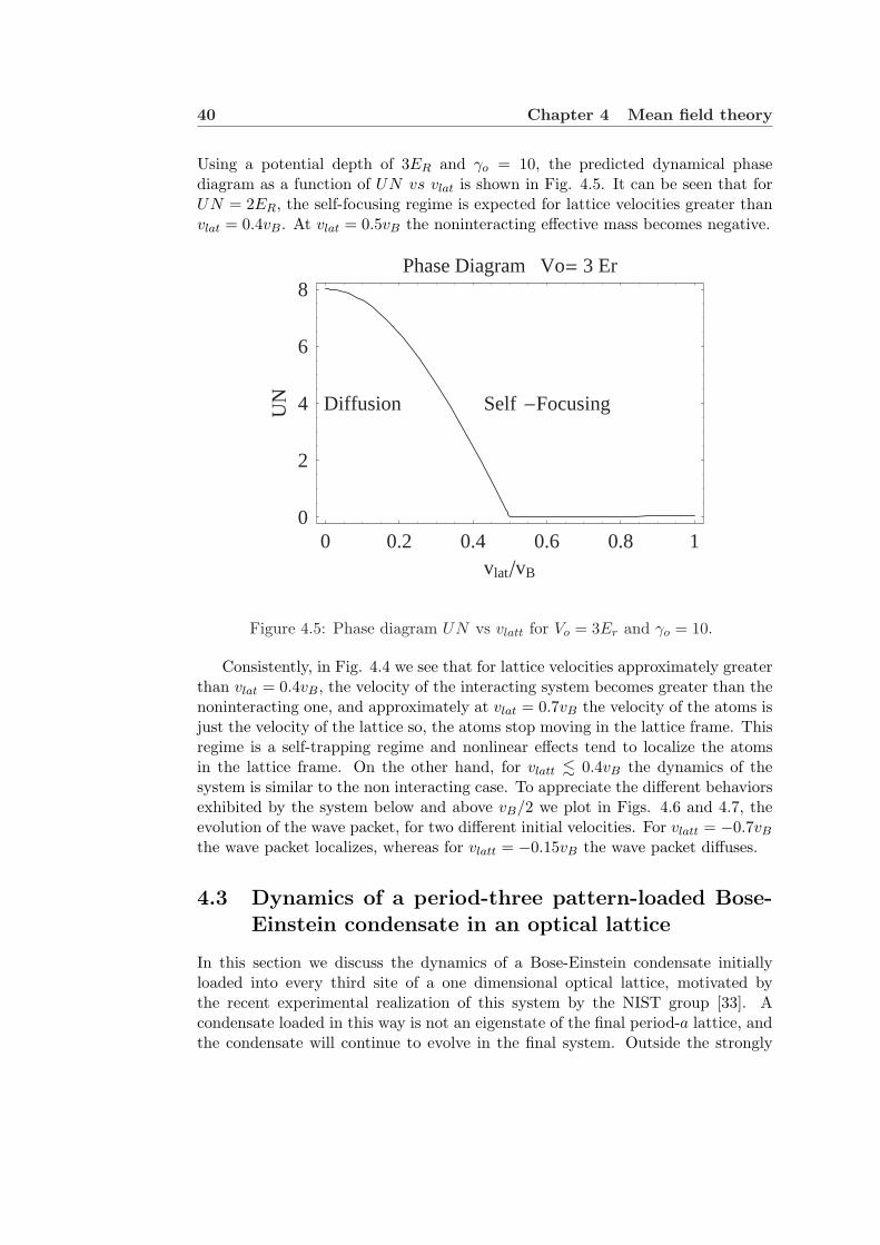
40 Chapter 4 Mean field theory
Using a potential depth of 3ER and γo = 10, the predicted dynamical phasediagram as a function of UN vs vlat is shown in Fig. 4.5. It can be seen that forUN = 2ER, the self-focusing regime is expected for lattice velocities greater thanvlat = 0.4vB. At vlat = 0.5vB the noninteracting effective mass becomes negative.
0 0.2 0.4 0.6 0.8 1vlatvB
0
2
4
6
8U
NPhase Diagram Vo= 3 Er
Diffusion Self -Focusing
Figure 4.5: Phase diagram UN vs vlatt for Vo = 3Er and γo = 10.
Consistently, in Fig. 4.4 we see that for lattice velocities approximately greaterthan vlat = 0.4vB, the velocity of the interacting system becomes greater than thenoninteracting one, and approximately at vlat = 0.7vB the velocity of the atoms isjust the velocity of the lattice so, the atoms stop moving in the lattice frame. Thisregime is a self-trapping regime and nonlinear effects tend to localize the atomsin the lattice frame. On the other hand, for vlatt . 0.4vB the dynamics of thesystem is similar to the non interacting case. To appreciate the different behaviorsexhibited by the system below and above vB/2 we plot in Figs. 4.6 and 4.7, theevolution of the wave packet, for two different initial velocities. For vlatt = −0.7vB
the wave packet localizes, whereas for vlatt = −0.15vB the wave packet diffuses.
4.3 Dynamics of a period-three pattern-loaded Bose-Einstein condensate in an optical lattice
In this section we discuss the dynamics of a Bose-Einstein condensate initiallyloaded into every third site of a one dimensional optical lattice, motivated bythe recent experimental realization of this system by the NIST group [33]. Acondensate loaded in this way is not an eigenstate of the final period-a lattice, andthe condensate will continue to evolve in the final system. Outside the strongly

4.3 Dynamics of a period-three pattern-loaded Bose-Einsteincondensate in an optical lattice 41
-30 0 30n
0
0.5
1
ÈznH
tLÈ2
t=30
-30 0 30n
00.5
11.5
ÈznH
tLÈ2
t=40
-30 0 30n
00.5
11.5
2
ÈznH
tLÈ2
t=50
-30 0 30n
0
0.5Èz
nHtLÈ2
t=0
-30 0 30n
0
0.5
ÈznH
tLÈ2
t=10
-30 0 30n
0
0.5
ÈznH
tLÈ2
t=20
Figure 4.6: Localization of the wave packet in the self-focusing regime vlatt =−0.7vB. Notice the change in the vertical scale in the last row
-60-30 0 30n
0
0.5
ÈznH
tLÈ2
t=30
-60-30 0 30n
0
0.5
ÈznH
tLÈ2
t=40
-60-30 0 30n
0
0.5
ÈznH
tLÈ2
t=50
-60-30 0 30n
0
0.5
ÈznH
tLÈ2
t=0
-60-30 0 30n
0
0.5
ÈznH
tLÈ2
t=10
-60-30 0 30n
0
0.5
ÈznH
tLÈ2
t=20
Figure 4.7: Evolution of the wave packet in the diffusive regime vlatt = −0.15vB.
correlated regime, the GPE equation is expected to give a good description ofthe condensate dynamics. In our system we assume the lattice is sufficiently deepthat a tight-binding description is applicable, and the DNLSE is valid. For theperiodic initial condition of equal wavefunction amplitude at every third site andzero at all others, symmetry arguments can be used to reduce the wavefunctionevolution to a two mode problem (analogous to a double well system with an energyoffset) for which an analytic solution of the dynamics can be given. We showthat for large ratios of the interatomic interaction strength to tunneling energythe condensate evolves with self-maintained population imbalance, whereby thecondensate population tends to remain localized in the initially occupied latticesites. A similar phenomenon has been studied in double-well systems [87, 88, 89,90, 91]. We show that the momentum distribution of an interacting condensatechanges in time in a manner which can be related to the spatial tunneling ofcondensate, and would be a suitable experimental observable.
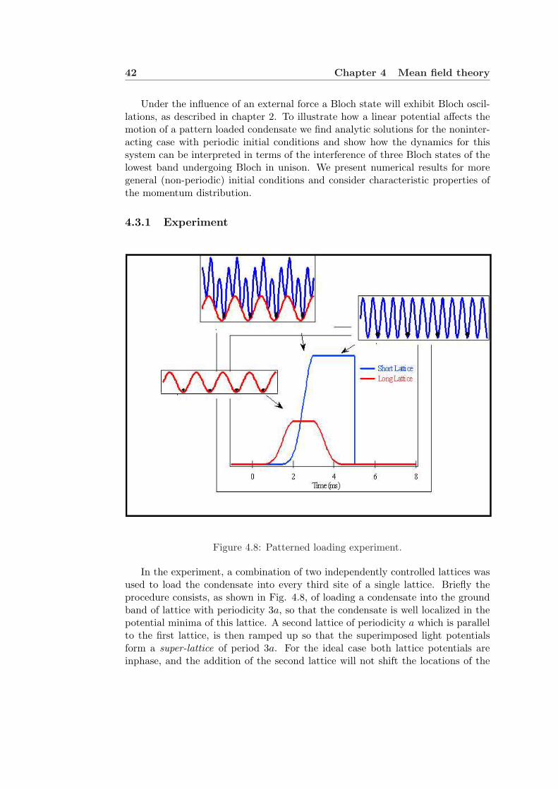
42 Chapter 4 Mean field theory
Under the influence of an external force a Bloch state will exhibit Bloch oscil-lations, as described in chapter 2. To illustrate how a linear potential affects themotion of a pattern loaded condensate we find analytic solutions for the noninter-acting case with periodic initial conditions and show how the dynamics for thissystem can be interpreted in terms of the interference of three Bloch states of thelowest band undergoing Bloch in unison. We present numerical results for moregeneral (non-periodic) initial conditions and consider characteristic properties ofthe momentum distribution.
4.3.1 Experiment
Figure 4.8: Patterned loading experiment.
In the experiment, a combination of two independently controlled lattices wasused to load the condensate into every third site of a single lattice. Briefly theprocedure consists, as shown in Fig. 4.8, of loading a condensate into the groundband of lattice with periodicity 3a, so that the condensate is well localized in thepotential minima of this lattice. A second lattice of periodicity a which is parallelto the first lattice, is then ramped up so that the superimposed light potentialsform a super-lattice of period 3a. For the ideal case both lattice potentials areinphase, and the addition of the second lattice will not shift the locations of the

4.3 Dynamics of a period-three pattern-loaded Bose-Einsteincondensate in an optical lattice 43
potential minima from those of the first lattice alone, and the condensate willremain localized at these positions. Finally, by removing the first period-3a latticeon a time scale long compared to band excitations, but short compared to thecharacteristic time of transport within the lattice, the condensate will be left inevery third site of the period-a lattice.
4.3.2 Case of no external potential
The major interest of this section is in the tunneling properties of the condensate inthe lattice, and in the noninteracting case the time scale for tunneling is determinedby the hopping matrix element J . For this reason it is convenient to define a newdimensionless scale of time τ = Jt/~, and dimensionless energy En = Vn/J andcoupling constant Λ = NU/J . In terms of these new variables the tight-bindingevolution equation (4.6) takes the form
i∂zn
∂τ= −(zn−1 + zn+1) + (En + Λ|zn|2)zn, (4.21)
• The case of periodic initial conditions: reduction to a two mode system
We treat first a model case in which no external potential is present, (En =0), and in which the initial occupancies of each third site are the same, and inwhich the condensate initially has a uniform phase. At τ = 0, the amplitudeszn(τ) are given by
z3n(0) =√
ρ, (4.22)z3n+1(0) = z3n+2(0) = 0, (4.23)
where ρ = 3/M with M the total number of lattice sites. Nρ representsthe initial number of atoms per occupied site. This initial condition is ho-mogeneous in the sense that each occupied site has the same amplitude andphase along the length of the lattice. For an infinite lattice, or one with peri-odic boundary conditions, the amplitudes for all initially occupied sites (z3n)evolve identically in time, and the amplitudes for the initially unoccupiedsites satisfy z3n+1(τ) = z3n+2(τ) for all τ and all n. This allows us to reducethe full set of equations (4.21) to a set of two coupled equations
i∂z0
∂τ= −2z1 + Λ|z0|2z0, (4.24)
i∂z1
∂τ= −(z1 + z0) + Λ|z1|2z1, (4.25)
where z3n ≡ z0 and z3n+1 = z3n+2 ≡ z1 for all n. The normalization condi-tion is
|z0|2 + 2|z1|2 = ρ. (4.26)

44 Chapter 4 Mean field theory
The Hamiltonian function, H, of this system is (from Eq. 4.8)
H =J
ρ
(− 2(z∗0z1 + z0z
∗1)− 2|z1|2 +
Λ2|z0|4
+Λ|z1|4)
(4.27)
=JΛρ
2.
By writing z0=ψ0√
ρ and z1=ψ1
√ρ/2, we can transform Eqs. (4.24)-(4.25)
to the form
i∂
∂τ
(ψ0
ψ1
)=
(γ|ψ0|2 −√2−√2 γ |ψ1|2√
2− 1
)(ψ0
ψ1
), (4.28)
where γ = Λρ is the ratio of on-site repulsion to tunneling energies, and thenormalization condition (4.26) is now |ψ0|2 + |ψ1|2 = 1. The factor of
√2
difference in the definition of ψ0 and ψ1 arises because ψ1 represents the am-plitude of the two initially unoccupied sites. With this factor incorporated,the matrix appearing in Eq. (4.28) is explicitly Hermitian. We note thatthis equation of motion is identical to that for a condensate in a double welltrap in the two mode approximation [92, 93].
We note in passing that a similar reduction, to a system of [m/2] + 1 equa-tions, exists for lattice systems that are loaded such that only every m-thsite is initially occupied.
• Solution of the equations of motion
It is convenient to write the lattice site amplitudes appearing in Eqs. (4.24)and (4.25) as z0=feiθ0
√ρ and z1= geiθ1
√ρ, where f, g, and θ are real. By
introducing the phase difference φ = θ0 − θ1, Eqs. (4.24), (4.25) and (4.27)can be recast as
.f = 2g sinφ, (4.29).g = −f sinφ, (4.30)γ
2= −4fg cosφ +
γ
2(f4 + 2g4
)− 2g2, (4.31)
The analytic solutions of Eqs. (4.29)-(4.31), found using a procedure similarto that presented by Raghavan et al. [87], can be expressed in terms ofWeierstrassian elliptic functions ℘(τ ; g2, g3) [69]. The analytic solutions are
f(τ) =
√1− 24
12℘(τ ; g2, g3) + (9 + 2γ + γ2), (4.32)
g(τ) =
√1− f(t)2
2, (4.33)

4.3 Dynamics of a period-three pattern-loaded Bose-Einsteincondensate in an optical lattice 45
where the parameters g2 and g3 are given by
g2 =(81− 14γ2 + 4γ3 + γ4
)/12, (4.34)
g3 =(729 + 243γ2 − 46γ3 − 15γ4 + γ6
)/216. (4.35)
The solutions f(τ) and g(τ) are oscillatory functions whose amplitudes andcommon period, T (γ), are determined by the parameter γ (see Figs. 4.9and 4.10). It is useful to qualitatively divide this behavior into two regimes,separated by γ = 2. Analysis of Eqs. (4.29) - (4.31) shows that f(τ0) = g(τ0)for some value of τ0 when γ ≤ 2, and for γ > 2, f(τ) > g(τ) for all τ .
Tunneling dominated regime
For γ . 2, we find that the oscillation period is essentially constant (see Fig.(4.9).
γ (J)
T (
h/J)
Figure 4.9: Oscillation period (in units of ~/J) as a function of the interactionstrength γ.
In this case the role of interactions is relatively small, and the behavior can beapproximately understood by taking γ = 0, in which case the matrix of Eq.(4.28) is constant in time. The equations of motion in this case are equivalentto those of a two-state Rabi problem [94], where the two levels are coupledby a Rabi frequency of strength
√2, which is detuned from resonance by
−1. This system will undergo Rabi oscillations whereby atoms periodicallytunnel from the initially occupied site into the two neighboring sites. Becausethe coupling is detuned from resonance the transfer of populations betweenwells is incomplete, with |ψ1|2 attaining a maximum value of 8/9. The Rabimodel predicts that the cycling frequency between the levels is equal to thedifference between the eigenvalues of the matrix of matrix of Eq. (4.28),which gives the period of oscillation as TRabi = 2π/3 in units of ~/J (see Fig.4.9).
Interaction dominated regime

46 Chapter 4 Mean field theory
The effect of interactions on the mean-field dynamics is to cause the energiesof the initially occupied sites to shift relative to those of the unoccupied sites.As γ increases and this energy shift increases relative to the strength of cou-pling between sites, the tunneling between sites occurs at a higher frequency,but with reduced amplitude. The population of the initially occupied sitesbecomes self trapped by the purely repulsive pair interaction, which in thecontext of a double well system has been called “macroscopic quantum selftrapping” [93]. This is demonstrated quantitatively in Fig. 4.10 where weplot the minimum value of f2 occurring during the oscillation as a functionof γ. In contrast to the tunneling dominated regime, where tunneling peri-odically populates all sites equally, the condensate tends to be localized onthe initially occupied sites in the interaction-dominated regime.
( )
γ (J)
Figure 4.10: Minimum value of f2 during an oscillation period as a function of γ.As γ increases the population imbalance between wells increases (see text).
• Momentum space dynamics
Typically the spacing between individual wells in an optical lattice is toosmall to resolve the localized density distributions of atoms in neighboringsites using standard imaging techniques.
The momentum distribution is a more convenient observable which approx-imately corresponds to the expanded spatial distribution of the releasedcondensate. Here we calculate the momentum dynamics of the condensateloaded into every third site of an optical lattice, and show how this relatesto the evolution of the spatial amplitudes given in Eqs. (4.32) and (4.33).
In the tight-binding approximation the condensate order parameter ϕ(x, τ)(4.4) is expressed as a sum over the lattice sites . Because of the periodicity ofthe system, the momentum space wavefunction, which we denote as ϕ(k, τ),is expressible as the Fourier series
ϕ(k, τ) =∑m
zm(τ)e−ikamχ(k), (4.36)

4.3 Dynamics of a period-three pattern-loaded Bose-Einsteincondensate in an optical lattice 47
whereχ(k) =
1√2π
∫ ∞
−∞e−ikxw0(x)dx. (4.37)
To compute the momentum distribution, we invoke the identity∑M−1
n=0 eikna =Mδk,2πm/a, where M is the number of lattice sites, and m an integer. Sincethere are only two independent amplitudes in the set zm, we find that
ϕ(k, τ) =√
3/ρcm(τ)χmδk,qm/3,
χm = χ(qm/3), (4.38)
cm(τ) =√
13ρ
(z0 + z1e
−iqm/3 + z2e−i2qm/3
),
where q is the reciprocal lattice vector q = 2π/a. The momentum distri-bution of the system has very sharp peaks of relative amplitude |cm|2 atmomentum k = qm/3, arising from the 3-lattice site spatial periodicity ofthe condensate wavefunction. In addition, χm describes a slowly varying en-velope determined by the localization of the Wannier states at each latticesite.
Using the analytic solutions for f and g, and Eq. (4.31), we obtain only twoindependent Fourier amplitudes
|c3n(τ)|2 =13
(1 +
γ
4(3f2 + 1)(f2 − 1)
), (4.39)
|c3n+1(τ)|2 =13
(1− γ
8(3f2 + 1)(f2 − 1)
)(4.40)
= |c3n+2(τ)|2. (4.41)
In the reduced zone scheme, where we only consider momenta in the rangek ∈ [−q/2, q/2], the momentum wavefunction then consists of three peakscorresponding to Bloch states of quasimomenta 0,±q/3. The identical be-havior of |c3n+1|2 and |c3n+2|2 means that the ±q/3 peaks always have thesame intensity. If interactions between the atoms are ignored (i.e. γ = 0),the momentum components are constant in time (see Eqs. (4.39) and (4.40)),even though tunneling occurs between the lattice sites. However, when in-teractions are considered, the momentum intensities explicitly depend on theoccupations of each site and will vary in time when tunneling occurs. Themagnitude of the time variation of the |cn|2 is proportional to γ, but willreduce for sufficiently large values of γ, where the self-trapping effect causesthe tunneling between lattice sites to stop (i.e. f2 ≈ 1 at all times). In Fig.4.11 we show the maximum contrast between the intensity of the Fourierpeaks, defined as ∆max ≡ (|c1|2 − |c0|2)max, where the value is maximizedby evaluating the |cn|2 at the time when f takes its minimum value (wenote that f(τ) is given by Eq. (4.32)). We note that the maximum contrastoccurs for γ ≈ 3.9; in this case, the zero quasimomentum component c0(τ)
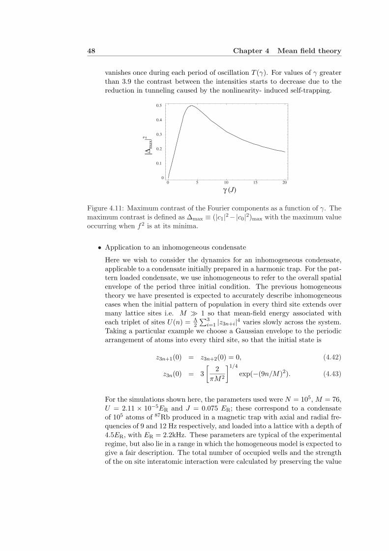
48 Chapter 4 Mean field theory
vanishes once during each period of oscillation T (γ). For values of γ greaterthan 3.9 the contrast between the intensities starts to decrease due to thereduction in tunneling caused by the nonlinearity- induced self-trapping.
0 5 10 15 20
0
0.1
0.2
0.3
0.4
0.5
|∆max|2
γ (J)
Figure 4.11: Maximum contrast of the Fourier components as a function of γ. Themaximum contrast is defined as ∆max ≡ (|c1|2−|c0|2)max with the maximum valueoccurring when f2 is at its minima.
• Application to an inhomogeneous condensate
Here we wish to consider the dynamics for an inhomogeneous condensate,applicable to a condensate initially prepared in a harmonic trap. For the pat-tern loaded condensate, we use inhomogeneous to refer to the overall spatialenvelope of the period three initial condition. The previous homogeneoustheory we have presented is expected to accurately describe inhomogeneouscases when the initial pattern of population in every third site extends overmany lattice sites i.e. M À 1 so that mean-field energy associated witheach triplet of sites U(n) = Λ
2
∑3i=1 |z3n+i|4 varies slowly across the system.
Taking a particular example we choose a Gaussian envelope to the periodicarrangement of atoms into every third site, so that the initial state is
z3n+1(0) = z3n+2(0) = 0, (4.42)
z3n(0) = 3[
2πM2
]1/4
exp(−(9n/M)2). (4.43)
For the simulations shown here, the parameters used were N = 105, M = 76,U = 2.11 × 10⁻⁵ER and J = 0.075 ER; these correspond to a condensateof 105 atoms of 87Rb produced in a magnetic trap with axial and radial fre-quencies of 9 and 12 Hz respectively, and loaded into a lattice with a depth of4.5ER, with ER = 2.2kHz. These parameters are typical of the experimentalregime, but also lie in a range in which the homogeneous model is expected togive a fair description. The total number of occupied wells and the strengthof the on site interatomic interaction were calculated by preserving the value

4.3 Dynamics of a period-three pattern-loaded Bose-Einsteincondensate in an optical lattice 49
of the chemical potential of the system upon reduction to one spatial dimen-sion and by assuming that each of the localized orbitals in the tight-bindingdescription are Gaussian. The hopping rate J was estimated by using Math-ieu functions. In Fig. 4.12 we show the evolution of the population of thecentral wells (normalized to one) compared with the homogeneous model
with γ taken to be the local mean field energy γeff = Λ√
2π (9/M).
Fig. 4.12 shows the results of numerical integration of the equations of motionand the approximate analytical solution given by the quasi-homogeneousmodel described above. We see that the numerical and analytical resultsagree well at short times, but differ more as time progresses due to thedifferent mean-field seen by different wells.
Figure 4.12: Comparison between the population evolution of the central threewells for the inhomogeneous condensate and the homogeneous model. Inhomoge-neous condensate: stars for the initially populated well and boxes for the initiallyempty wells. Homogeneous model: dashed line represents the initially populatedwells, and the solid line represented the initially unpopulated wells. We used γeff
as the local mean field energy (see text). The parameters used for the simulationwere J = 0.075ER and γeff = 2.64.
To understand the disagreement as time evolves, we show in Fig. 4.13 thenumerical Fourier spectrum for the inhomogeneous case evaluated at severaldifferent times. The variation of the intensities of the peaks, which, as shownbelow, is related to the spatial tunneling between lattice sites in the presenceof the mean field, can be seen in the plot. Initially all occupied sites are inphase and the three distinctive momentum peaks have a narrow width deter-mined by the intrinsic momentum uncertainty of the condensate envelope.That is the reason why the homogeneous model fits very well. However, astime progresses the mean field variation across the lattice causes the tun-neling rates to vary with position and leads to momentum peak broadening.This effect eventually causes the homogeneous model to become an inaccu-rate description of the inhomogeneous system.
We note that momentum space signature for spatially tunneling in the in-
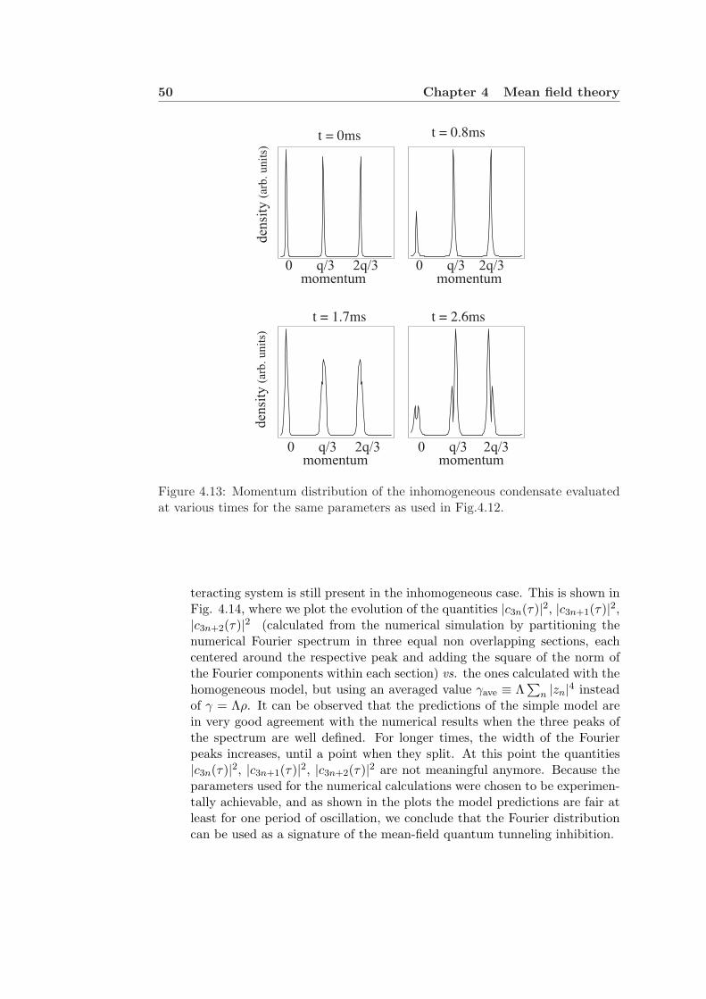
50 Chapter 4 Mean field theory
t = 1.7ms t = 2.6ms
t = 0ms t = 0.8ms
momentum momentum
den
sity
(ar
b. unit
s)
0 q/3 2q/3 0 q/3 2q/3
den
sity
(ar
b. unit
s)
momentum momentum0 q/3 2q/3 0 q/3 2q/3
Figure 4.13: Momentum distribution of the inhomogeneous condensate evaluatedat various times for the same parameters as used in Fig.4.12.
teracting system is still present in the inhomogeneous case. This is shown inFig. 4.14, where we plot the evolution of the quantities |c3n(τ)|2, |c3n+1(τ)|2,|c3n+2(τ)|2 (calculated from the numerical simulation by partitioning thenumerical Fourier spectrum in three equal non overlapping sections, eachcentered around the respective peak and adding the square of the norm ofthe Fourier components within each section) vs. the ones calculated with thehomogeneous model, but using an averaged value γave ≡ Λ
∑n |zn|4 instead
of γ = Λρ. It can be observed that the predictions of the simple model arein very good agreement with the numerical results when the three peaks ofthe spectrum are well defined. For longer times, the width of the Fourierpeaks increases, until a point when they split. At this point the quantities|c3n(τ)|2, |c3n+1(τ)|2, |c3n+2(τ)|2 are not meaningful anymore. Because theparameters used for the numerical calculations were chosen to be experimen-tally achievable, and as shown in the plots the model predictions are fair atleast for one period of oscillation, we conclude that the Fourier distributioncan be used as a signature of the mean-field quantum tunneling inhibition.

4.3 Dynamics of a period-three pattern-loaded Bose-Einsteincondensate in an optical lattice 51
Figure 4.14: Evolution of momentum peak populations. Upper curves: populationof the q = ±2π/3 momentum states. Lower curves: population of the q = 0momentum state. Inhomogeneous condensate (dotted), homogeneous result (solidline), where the comparison is made by replacing γ by an average mean field energyγave ≡ Λ
∑n |zn|4 = 1.85. Parameters are the same as in Fig. 4.12.
4.3.3 Dynamics with a constant external force
• Homogeneous three state model
In this section we consider the dynamics of a periodically loaded condensatein the presence of a linear external potential, corresponding to a uniform forceparallel to the lattice. In what follows we assume that the force is sufficientlyweak that band excitations due to Landau-Zener tunneling are negligible, sothat a tight-binding picture of the lowest band is sufficient to describe thedynamics. In this case the evolution equation differs from what we consideredin the previous section by the term En in Eq. (4.21) taking the form En =nξ, where ξ is the potential difference between lattice sites (in units of thehopping matrix element J). Taking the initial conditions (4.22)-(4.23), andtransforming the Wannier amplitudes as z3n+j(τ) = Ψ3n+j(τ)e−i3nξτ (j =0, 1, 2), we obtain the evolution equations
i∂Ψ3n
∂τ= −(Ψ3n−1e
i3ξτ + Ψ3n+1)
+Λ|Ψ3n|2Ψ3n, (4.44)
i∂Ψ3n+1
∂τ= −(Ψ3n+2 + Ψ3n) + ξΨ3n+1
+Λ|Ψ3n+1|2Ψ3n+1, (4.45)
i∂Ψ3n+2
∂τ= −(Ψ3n+1 + Ψ3n+3e
−i3ξτ ) + 2ξΨ3n+1
+Λ|Ψ3n+1|2Ψ3n+1. (4.46)
Assuming periodic boundary conditions, the periodicity of the initial condi-tions and equations of evolution allow considerable simplification from the
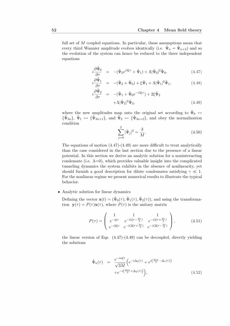
52 Chapter 4 Mean field theory
full set of M coupled equations. In particular, these assumptions mean thatevery third Wannier amplitude evolves identically (i.e. Ψn = Ψn+3) and sothe evolution of the system can hence be reduced to the three independentequations
i∂Ψ0
∂τ= −(Ψ2e
i3ξτ + Ψ1) + Λ|Ψ0|2Ψ0, (4.47)
i∂Ψ1
∂τ= −(Ψ2 + Ψ0) + ξΨ1 + Λ|Ψ1|2Ψ1, (4.48)
i∂Ψ2
∂τ= −(Ψ1 + Ψ0e
−i3ξτ ) + 2ξΨ2
+Λ|Ψ2|2Ψ2, (4.49)
where the new amplitudes map onto the original set according to Ψ0 ↔Ψ3n, Ψ1 ↔ Ψ3n+1, and Ψ2 ↔ Ψ3n+2, and obey the normalizationcondition
2∑
j=0
|Ψj |2 =3M
. (4.50)
The equations of motion (4.47)-(4.49) are more difficult to treat analyticallythan the case considered in the last section due to the presence of a linearpotential. In this section we derive an analytic solution for a noninteractingcondensate (i.e. Λ=0), which provides valuable insight into the complicatedtunneling dynamics the system exhibits in the absence of nonlinearity, yetshould furnish a good description for dilute condensates satisfying γ ¿ 1.For the nonlinear regime we present numerical results to illustrate the typicalbehavior.
• Analytic solution for linear dynamics
Defining the vector x(t) = (Ψ0(τ), Ψ1(τ), Ψ2(τ)), and using the transforma-tion y(τ) = P (τ)x(τ), where P (τ) is the unitary matrix
P (τ) =
1 1 1e−iξτ e−i(ξτ− 2π
3) e−i(ξτ+ 2π
3)
e−i2ξτ e−i(2ξτ+ 2π3
) e−i(2ξτ− 2π3
)
, (4.51)
the linear version of Eqs. (4.47)-(4.49) can be decoupled, directly yieldingthe solutions
Ψn(τ) =e−inξτ
√3M
(e−i∆0(τ) + ei( 2nπ
3−∆1(τ))
+e−i( 2nπ3
+∆2(τ))), (4.52)

4.3 Dynamics of a period-three pattern-loaded Bose-Einsteincondensate in an optical lattice 53
where we have defined the phase terms
∆n(τ) = −2ξ
[sin(ξτ − 2nπ
3) + sin(
2nπ
3)]
, (4.53)
for n = 0, 1, 2.
These solutions for the spatial amplitudes Ψi(τ) can be most easily under-stood by considering a Bloch state decomposition of the condensate wave-function. The nature of our system allows us to construct an analytic formfor the initial wavefunction. Because the system has a three lattice site periodand is assumed to be in the lowest band, the wavefunction can be expressedas a superposition of three Bloch waves (of the lowest band) which are sym-metrically spaced in quasimomentum. Assuming the condensate initially hasa total crystal momentum of zero, at this time the wavefunction must be ofthe form
ϕ(x, 0) = α0φ0(x) + α+φq/3(x) + α−φ−q/3(x), (4.54)
where φk(x) is a Bloch state with quasimomentum k, and the α are complexconstants determined by the lattice depth, with |α+| = |α−|.The action of an external force on a Bloch state causes it to linearly changeits quasimomentum in time according to
k(τ) = − ξ
aτ + k(0). (4.55)
The periodicity of the Bloch dispersion relation in k, and hence of the groupvelocity of the Bloch wave, gives rise to the well-known phenomenon of Blochoscillations (see chapter 2). For the case we are considering here, the systemconsists of three Bloch states whose quasimomenta will translate in unisonunder the action of the external force. During this evolution each stateaccumulates phase at a rate determined by the instantaneous Bloch energy,i.e.
∆n(τ) =∫ τ
0E(kn(s))ds, (4.56)
where kn(τ) = −ξτ/a+kn(0) is the quasimomentum of Bloch state n at timet. In the tight-binding approximation the dispersion relation for the Blochstates has the analytic form
E(k) = −2 cos(ka), (4.57)
for which ∆n(τ) can be evaluated, and yields the results given in Eqs. (4.53)).The wavefunction evolution in the Bloch basis is
ϕ(x, τ) = α0φ− ξat(x)e−i∆0(τ) + α+φ− ξ
at+ q
3(x)e−i∆1(τ)
+α−φ− ξat− q
3(x)e−i∆2(τ). (4.58)

54 Chapter 4 Mean field theory
From this solution we can obtain solutions for the evolution of the spatialamplitudes Eqs. (4.52). To do this we expand the Bloch states in terms ofWannier functions according to, φk(x) =
∑n eiknaw0(x−na) (see chapter 2)
and make use of Eq. (4.5). Note: we take all α = ρ3 as determined by the
initial conditions, Eqs.(4.22) and (4.23).
Bloch OscillationsThe evolution of the spatial amplitudes, and in particular the populationin each well is then determined by the interference of the Bloch phases∆n. These functions are all periodic in time with period τB = 2π/ξ (inunits of τ = tJ/~). This is the normal Bloch oscillation period, andgives the time scale over which the quasimomenta of the Bloch statesincreases by exactly one reciprocal lattice vector.
Small ξ solution - Non classical transportTo understand the dynamics, we first start by considering the case whenξ is small. For this case, the population in the wells is given by
|Ψ0(τ)|2 =1
3M
(5 + 4 cos(3τ) + ξ2h(τ)
)(4.59)
|Ψ1(τ)|2 =1
3M
((2 + 3ξ)[1− cos(3τ)− ξ2
2h(τ)]
)(4.60)
|Ψ2(τ)|2 =1
3M
((2− 3ξ)[1− cos(3τ)− ξ2
2h(τ)]
)(4.61)
where
h(τ) =τ3
2(6τ + 3τ cos(3τ)− 4 sin(3τ)) . (4.62)
The above solution shows that when the force is applied, the degeneracyin the population of the wells represented by Ψ1 and Ψ2 is lifted. Forξ > 0, atoms in Ψ0 start to tunnel to Ψ1 more rapidly than to Ψ2. Thisshould be compared with the results in the absence of the force, whereΨ1 and Ψ2 behave identically. Thus, in this weak limit, the effect of alinear potential is to enhance the tunneling from the initial populated3n wells to their 3n + 1 neighbors ones, making the system closer toresonance, in the sense of Eq. (4.28), where the resonance conditionresults in the initially populated wells becoming empty at some latertime. It is interesting to note that the system exhibits ”nonclassical”dynamics whereby the atoms start to tunnel in the direction oppositethe direction of the force (this statement applies even when the externalfield is not weak).
ResonancesIn Fig. 4.15 we show the temporal evolution of the spatial amplitudes Ψi
for a range of values of ξ. For certain choices of ξ the initially occupiedΨ0 amplitude periodically disappears - we refer to these as resonances.
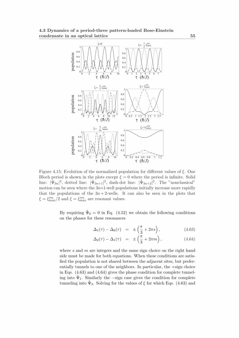
4.3 Dynamics of a period-three pattern-loaded Bose-Einsteincondensate in an optical lattice 55
0
ξ =5
14ξ ξ =3ξ
ξ=2
7ξ ξ = ξ
τ
0
ξ=0
0
ξ=1
2ξ
(h/J) τ (h/J)
τ (h/J) τ (h/J)
τ (h/J) τ (h/J)
Figure 4.15: Evolution of the normalized population for different values of ξ. OneBloch period is shown in the plots except ξ = 0 where the period is infinite. Solidline: |Ψ3n|2, dotted line: |Ψ3n+1|2, dash-dot line: |Ψ3n+2|2. The ”nonclassical”motion can be seen where the 3n+1-well populations initially increase more rapidlythat the populations of the 3n+2-wells. It can also be seen in the plots thatξ = ξres
max/2 and ξ = ξresmax are resonant values.
By requiring Ψ0 = 0 in Eq. (4.52) we obtain the following conditionson the phases for these resonances
∆1(τ)−∆0(τ) = ±(π
3+ 2πs
), (4.63)
∆2(τ)−∆1(τ) = ±(π
3+ 2πm
), (4.64)
where s and m are integers and the same sign choice on the right handside must be made for both equations. When these conditions are satis-fied the population is not shared between the adjacent sites, but prefer-entially tunnels to one of the neighbors. In particular, the +sign choicein Eqs. (4.63) and (4.64) gives the phase condition for complete tunnel-ing into Ψ1. Similarly the −sign case gives the condition for completetunneling into Ψ2. Solving for the values of ξ for which Eqs. (4.63) and
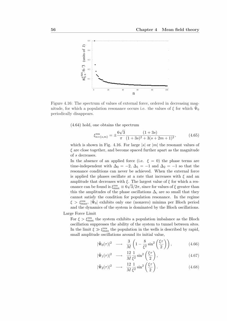
56 Chapter 4 Mean field theory
0 20 40 60 80 100
n
0.1
0.2
0.3
0.4
0.5
Figure 4.16: The spectrum of values of external force, ordered in decreasing mag-nitude, for which a population resonance occurs i.e. the values of ξ for which Ψ0
periodically disappears.
(4.64) hold, one obtains the spectrum
ξresn=(s,m) = ±6
√3
π
(1 + 3s)(1 + 3s)2 + 3(s + 2m + 1)2
, (4.65)
which is shown in Fig. 4.16. For large |s| or |m| the resonant values ofξ are close together, and become spaced further apart as the magnitudeof s decreases.In the absence of an applied force (i.e. ξ = 0) the phase terms aretime-independent with ∆0 = −2, ∆1 = −1 and ∆2 = −1 so that theresonance conditions can never be achieved. When the external forceis applied the phases oscillate at a rate that increases with ξ and anamplitude that decreases with ξ. The largest value of ξ for which a res-onance can be found is ξres
max ≡ 6√
3/2π, since for values of ξ greater thanthis the amplitudes of the phase oscillations ∆i are so small that theycannot satisfy the condition for population resonance. In the regimeξ > ξres
max, |Ψ0| exhibits only one (nonzero) minima per Bloch periodand the dynamics of the system is dominated by the Bloch oscillations.
Large Force LimitFor ξ > ξres
max the system exhibits a population imbalance as the Blochoscillation suppresses the ability of the system to tunnel between sites.In the limit ξ À ξres
max the population in the wells is described by rapid,small amplitude oscillations around its initial value,
|Ψ0(τ)|2 −→ 3M
(1− 8
ξ2sin2
(ξτ
2
)), (4.66)
|Ψ1(τ)|2 −→ 12M
1ξ2
sin2
(ξτ
2
), (4.67)
|Ψ2(τ)|2 −→ 12M
1ξ2
sin2
(ξτ
2
). (4.68)
4.3 Dynamics of a period-three pattern-loaded Bose-Einsteincondensate in an optical lattice 57
The case of ξ = 3ξresmax depicted in Fig.4.15 shows an approach to this
behavior.
• Numerical results for the non-linear case
(h/J)
(h/J)
Figure 4.17: Effects of interactions on generalized Bloch oscillations for the patternloaded system. Evolution of |Ψn|2 for various interaction strengths. Upper plot:ξ = 2ξres
max. Lower plot: ξ = 2ξresmax/7.
Because of the difficulty of solving analytically the equations of motion thenonlinear equations were solved numerically. Although the dynamics in thissituation is considerably more complicated than in the linear case, the reso-nance picture still gives us useful guidance concerning the expected behavior.In general, there exist critical values of ξ and Λ above which no resonances oc-cur. Furthermore, nonlinearity tends to destroy the periodicity of the Blochoscillations that is present in the noninteracting case. For example, in Fig.4.17, we see that for ξ = 2ξres
max, the introduction of interactions brings the

58 Chapter 4 Mean field theory
system into resonance, but that for large interaction strength, nonresonantbehavior is restored. For ξ = 2ξres
max/7, on the other hand, the introductionof interactions eventually draws the system out of resonance.
Concerning the momentum distribution, similarly to the untilted case, inter-atomic interactions induce time variation of the momentum intensities. Thecontrast between momentum components vanishes at Λ = 0. As Λ increases,the contrast increases to a maximum value, then eventually decreases towardszero when macroscopic imbalance is achieved, analogous to what is seen inFig. 4.11 for the untilted case. Because the external field together with thenonlinearity breaks down the periodicity of time evolution, the dynamics ofthe momentum distribution is quite complex.
To compare the predictions of the homogeneous model in the presence of alinear external potential to a more realistic case, we again solved numericallythe discrete nonlinear Schrodinger equation for a condensate loaded intoevery third lattice site but, instead of being homogeneous, initially with aGaussian profile. Very good agreement between the model and the numericalresults was found for short times and modest mean-field energies, if, as in theuntilted case, we use an effective mean field energy. In Figs. 4.18 and 4.19we present a comparison between the evolution of the normalized populationat the central wells found numerically and the prediction of the model for theparameters: NU = 4.8ER, M = 290, J = 0.075 ER and ξ = 2. For longertimes, the model predictions start to disagree with numerical simulation dueto the spread of the three Fourier peaks. We observe that the dynamics aremuch more sensitive to inhomogeneous effects in the presence of an externalforce, and for the more inhomogeneous initial state used in Figs. (4.12 -4.14) (which extends over M = 76 sites), the inhomogeneous result muchmore rapidly departs from the homogeneous prediction than the examplepresented here.
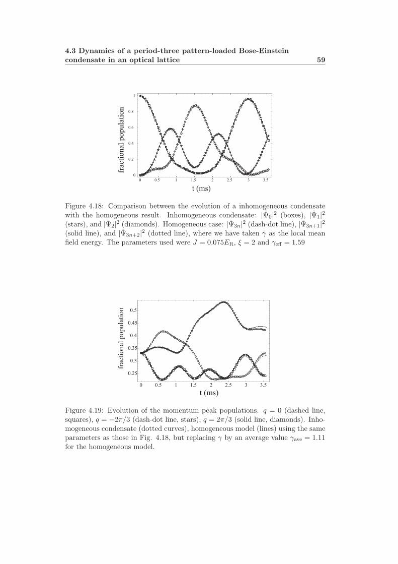
4.3 Dynamics of a period-three pattern-loaded Bose-Einsteincondensate in an optical lattice 59
Figure 4.18: Comparison between the evolution of a inhomogeneous condensatewith the homogeneous result. Inhomogeneous condensate: |Ψ0|2 (boxes), |Ψ1|2(stars), and |Ψ2|2 (diamonds). Homogeneous case: |Ψ3n|2 (dash-dot line), |Ψ3n+1|2(solid line), and |Ψ3n+2|2 (dotted line), where we have taken γ as the local meanfield energy. The parameters used were J = 0.075ER, ξ = 2 and γeff = 1.59
Figure 4.19: Evolution of the momentum peak populations. q = 0 (dashed line,squares), q = −2π/3 (dash-dot line, stars), q = 2π/3 (solid line, diamonds). Inho-mogeneous condensate (dotted curves), homogeneous model (lines) using the sameparameters as those in Fig. 4.18, but replacing γ by an average value γave = 1.11for the homogeneous model.

60 Chapter 4 Mean field theory
Chapter 5
Quadratic approximations
As discussed in chapter 3, the Bose-Hubbard Hamiltonian is an appropriate model,when the loading process produces atoms in the lowest vibrational state of eachwell, with a chemical potential smaller than the energy gap to the first vibrationallyexcited state. The quartic form of the Hamiltonian makes it very difficult to dealwith it in all the different regimes. The aim of this chapter is to rewrite it so thata systematic approach can be developed in the weakly interacting regime, whena condensate is present. The basic idea, which was first proposed by Bogoliubovin 1947 [11], is to treat the field operator as a c-number plus a fluctuating term.The c-number describes the condensate or the coherent part of the matter field.In the weakly interacting regime, quantum fluctuations are small, and thereforethe dominant terms in the Hamiltonian are quadratic in the fluctuating field. Thenon-quadratic terms should be of higher order and can be treated perturbatively.
In this chapter, we apply the Bogoliubov approximation to the Bose- Hub-bard Hamiltonian and derive the correspondent Bogoliubov-de Genes(BdG) equa-tions as developed in Refs. [77, 95]. We also deal with the higher order termsby considering different approximations. Among them we discuss the Hartree-Fock-Bogoliubov (HFB) approximation, the HFB-Popov approximation and theimproved Popov approximation where the bare potential is upgraded to the many-body scattering matrix. All of these approximate approaches are valid only inthe weakly interacting regime when quantum fluctuations are small. They willfail to give a good description as interactions become important and the systemapproaches the Mott insulator transition. To test the validity of the approxima-tions we compared them with numerical solutions obtained by diagonalizing theBose-Hubbard Hamiltonian.
In this chapter we also derive an explicit expression for the superfluid densitybased on the rigidity of the system under phase variations. We show how thesuperfluid fraction can be thought of as a natural order parameter to describe thesuperfluid to Mott insulator transition.
Because we are interested in the quantum effects caused by interactions thatdrive the quantum phase transition instead of thermal quantum fluctuations, theanalysis in the present chapter is going to be restricted to the zero temperature
62 Chapter 5 Quadratic approximations
case.
5.1 The characteristic Hamiltonian
In the very weakly interacting regime, to a good approximation, the creation andannihilation operators on each site can be replaced by a c-number(see chapter4). To include the small quantum fluctuations in the description of the systemwe assume that the field operator can be written in terms of a c-number plus afluctuation operator:
an = zn + ϕn. (5.1)
Replacing this expression for an in the Bose-Hubbard Hamiltonian Eq. (3.4)leads to :
H = H0 + H1 + H2 + H3 + H4, (5.2)
with
H0 = −J∑
<n,m>
z∗nzm +∑n
[(Vn − µ)|zn|2 +
U
2|zn|4
], (5.3)
H1 = −J∑
<n,m>
ϕnz∗m +∑
n
(Vn − µ + U |zn|2
)z∗nϕn + h.c., (5.4)
H2 = −J∑
<n,m>
ϕ†nϕm +∑
n
(Vn − µ)ϕ†nϕn +
U
2
∑n
(ϕ2†
n z2n + ϕ2
nz2∗n + (ϕ†nϕn + ϕnϕ†n)|zn|2
), (5.5)
H3 = U∑
n
ϕ†nϕ†nϕnzn + h.c., (5.6)
H4 =U
2
∑n
ϕ†nϕ†nϕnϕn. (5.7)
Where < n,m > restricts the sum over m to nearest neighbors and h.c. standsfor the hermitian conjugate. The terms of the Hamiltonian have been groupedin equations according to the number of non condensate operators which theycontain.
5.2 Bogoliubov-de Gennes (BdG) equations
In this section we neglect higher order terms and focus only on the quadraticHamiltonian. The first step in the diagonalization is the minimization of the energyfunctional H0 . This requires the condensate amplitudes zn to be a stationarysolution of the DNLSE (4.6), which in turn means that the linear Hamiltonian H1
vanishes. For the time independent situation the DNLSE can be written as
µzn = −J∑
<m,n>
zm + (Vn + U |zn|2)zn (5.8)

5.2 Bogoliubov-de Gennes (BdG) equations 63
The Hamiltonian H0 gives a description which includes only the contribution fromthe condensate. The quadratic Hamiltonian H2 allows the leading order effects ofthe non condensate to be taken into account. By including second order terms inthe Hamiltonian two classes of interactions are included besides the condensate-condensate ones: a) Interactions between one excited atom and one condensateatom leading to transitions of the form |0j〉 → |0i〉 (direct and exchange excita-tions)and b) interactions between two condensate atoms which cause the atoms tobe excited to non condensate states |00〉 → |ij〉 (pair excitations). Schematicallythey are shown in fig.5.1.
Figure 5.1: Scattering processes included in the quadratic hamiltonian: a) Directand exchange excitations, b) Pair excitations
The quadratic Hamiltonian can be diagonalized by finding a basis of so-calledquasiparticle states which do not interact which each other. Mathematically thisinvolves a linear canonical transformation of the single-particle creation and annihi-lation operators a†n and an into quasiparticle operators α†s, αs. The transformationis known as Bogoliubov transformation and is given by
ϕn =∑
s6=0
(us
nαs − v∗sn α†s)
. (5.9)
In general the spectrum of fluctuations includes a zero mode. This mode is theGoldstone boson associated with the breaking of global phase invariance by thecondensate. The zero mode is essentially non perturbative and it introduces anartificial infrared divergence in low dimensional models. For this reason quadraticapproximations are actually improved if the contribution from this mode is ne-glected all together [96]. A different way to deal with the zero mode has beenproposed by Castin and Dum [98], Gardiner [97] and Morgan [16]. Here the the-ory is written in terms of operators which exchange particles between zero and

64 Chapter 5 Quadratic approximations
nonzero modes, conserving the total particle number, and one further operatorwhich changes total particle number. As shown by [16] both the latter and theformer approaches lead to the same physical predictions, so for simplicity we aregoing to ignore zero mode fluctuations and restrict the fluctuation operators to actonly on the excited states.
The Bogoliubov transformation Eq. (5.9) is required to be canonical, whichmeans that it preserves the commutation relations and leads to bosonic quasipar-ticles. To satisfy this, the amplitudes us
n, vsn are constrained by the conditions:
∑n
(u∗sn us′
n − v∗sn vs′n
)= δss′, (5.10)
∑n
(us
nvs′n − v∗sn u∗s′n
)= 0. (5.11)
The necessary and sufficient conditions that the quasiparticle amplitudes have tofulfill to diagonalize the Hamiltonian are provided by the so called Bogoliubov-deGennes (BdG) equations
( L MM∗ L
)(us
vs
)= ωB
s
(us
−vs
)+ cs
(z−z∗
), (5.12)
with us = (us1, u
s2, ...) , vs = (vs
1, vs2, ...) and z = (z1, z2, ...). The matrices L and
M are given by
Lnm = −J∑
<n,l>
δnlδlm + δnm(2U |zn|2 + Vn − µ) (5.13)
Mnm = −Uz2i δnm. (5.14)
with δnl the Kronecker delta which is one if n = l and zero otherwise. The param-eters cs ensure that the solutions with ωB
s 6= 0 are orthogonal to the condensate[16]. These parameters are given by
cs = U
∑n |zn|2(z∗nus
n − znvsn)∑
n |zn|2 (5.15)
The BdG equations without the cs parameters have the same quasiparticle energiesas Eq.(5.12), nevertheless the solutions are orthogonal to the condensate only inthe general sense, i.e.
∑n(z∗nus
n − znvsn) = 0. Each of the terms,
∑n z∗nus
nand∑n znvs
n are not necessarily zero. To obtain the desired orthogonal modes oneway to proceed is to solve the BdG equations setting the cs to zero and thento remove from the solutions their projection onto the condensate. If the BdGequations are satisfied, the quadratic Hamiltonian takes the form
H2 =∑
s 6=0
[ωB
s α†sαs +12
(ωB
s − Lss
)]. (5.16)

5.3 Higher order terms 65
If the Hamiltonian H2, is positive definite, which is the case when the condensateamplitudes correspond to a stable state of the system, the eigenvalues of the systemare real. The solutions ωB
s come in pairs with positive and negative energies, ifωB
s is a solution for the amplitudes (us,vs) then −ωBs is also a solution for the
amplitudes (vs∗,us∗). There is always a solution with ωBs = 0 and in this case the
amplitudes must be proportional to the condensate (v0,u0) ∝ (z, z). We explicitlyexclude the zero mode solution to guarantee that the excitations are orthogonalto the condensate.
To have a complete description of the quadratic Hamiltonian, we define the onebody density fluctuation matrix, ρnm and the anomalous average matrix, mnm as:
ρnm = 〈a†nam〉 − 〈a†n〉〈am〉 = 〈ϕ†nϕm〉, (5.17)mnm = 〈anam〉 − 〈an〉〈am〉 = 〈ϕnϕm〉. (5.18)
The averages denotes an ordinary quantum expectation value. At zero tempera-ture, the average is over the ground quasiparticle state given by αs|0〉 = 0 and theρnm and mnm can be written in terms of quasiparticle amplitudes as:
ρnm =∑
s6=0
vs∗n vs
m, (5.19)
mnm = −∑
s6=0
usnvs∗
m . (5.20)
Physically, the quantity ρnn represents the non -condensate population (or deple-tion) at position n or depletion at position n. If the average number of atoms isN , the depletion and condensate atoms are related by the equation:
N =∑
n
⟨a†nan
⟩=
∑n
(|zn|2 + ρnn
). (5.21)
The interpretation to the physical meaning of the anomalous term is postponed tosection 5.7.2.
5.3 Higher order terms
In the preceding section we described the diagonalization of the Hamiltonian con-taining only terms up to quadratic order in the field operators. We now wantto go beyond this approximation and consider the corrections introduced by thecubic and quartic terms. Taking into account higher order terms we are mainlyintroducing many-body effects on the scattering.
66 Chapter 5 Quadratic approximations
5.3.1 Hartree-Fock-Bogoliubov equations
Third and quartic terms in the Hamiltonian can be included by treating themin a self-consistent mean field approximation, which relies upon the factorizationapproximation: products of many operators are approximated by paring the oper-ators in all possible ways and replacing these pairs by their expectation value [15].Using the factorization approximation, one can reduce third and quartic productsof fluctuation field operators to:
ϕ†nϕnϕn → 2ρnnϕn + 2mnnϕ†n, (5.22)ϕ†nϕ†nϕnϕn → 4ρnnϕ†nϕn + mnnϕ†nϕ†n + m∗
nnϕnϕn − (2ρ2nn + |mnn|2).(5.23)
Eq.(5.23) is justified by Wick’s theorem [51], which gives 〈ϕ†nϕ†nϕnϕn〉 = 2ρ2nn +
|mnn|2, while Eq.(5.22) is justified by analogy [16].Therefore, using Eq.(5.23) and Eq.(5.22) in H3 and H4 ( Eqs. (5.6) and (5.7)) onecan reduce them to quadratic forms in terms of the functions ρnm and mnm. Thec-number term in Eq.(5.23) introduces also a energy shift in H0 :
∆H0 =U
2(2ρ2
nn + |mnn|2) (5.24)
H3 = U∑
n
(2ρnnϕn + mnnϕ†n)zn + h.c., (5.25)
H4 =U
2
∑n
(2ρnnϕ†nϕn + mnnϕnϕn) + h.c.. (5.26)
The corrections from higher order terms yield a modified quadratic Hamiltonianwhich can be also diagonalized. The diagonalization leads to the following equa-tions
µHFBzn = −J∑
<m,n>
zm + (Vn + U |zn|2 + 2Uρnn + Umnn)zn, (5.27)
( LHFB MHFB
M∗HFB L∗HFB
)(us
vs
)= ωHFB
s
(us
−vs
)+
(cHFB−s z
−cHFB+
s z∗
), (5.28)
LHFBnm = −J
∑
<n,l>
δnlδlm + δnm(2U |zn|2 + Vn − µHFB + 2Uρnn), (5.29)
MHFBnm = −(Uz2
i + Umnn)δnm, (5.30)
cHFB∓s =
U∑
n |zn|2(z∗nusn − znvs
n)∓ U∑
n (m∗nnznus
n −mnnz∗nvsn)∑
n |zn|2 .(5.31)
The parameters cHFB∓s are there again to enforce the orthogonality of the quasi-
particle modes with the condensate [16].
5.4 The Bose-Hubbard model and superfluidity 67
The above set of equations (5.27) to (5.30) are known as Hartree-Fock-Bogoliubov(HFB) equations. Even though they take into account higher order corrections,they have the problem that violate the Hugenholtz and Pines theorem [99] whichstates that the energy spectrum of a Bose gas is gapless, i.e, there exists an exci-tation with an energy which tends to zero as the momentum tends to zero.
5.3.2 HFB-Popov approximation
One way to solve the gap problem is to set the anomalous term mnn to zeroin HFB equations. This procedure is known as HFB-Popov approximation. TheHFB-Popov equations were first introduced by Popov [52], and they are consideredto be a better approximation than the HFB equations because they yield a gaplessspectrum.
The HFB-Popov equations have the form:
µP zn = −J∑
<m,n>
zm + (Vn + U |zn|2 + 2Uρnn)zn, (5.32)
( LP MP
M∗P L∗P)(
us
vs
)= ωP
s
(us
−vs
)+ cs
(z−z∗
), (5.33)
LPnm = −J
∑
<n,l>
δnlδlm + δnm(2U |zn|2 + Vn − µP + 2Uρnn), (5.34)
MPnm = −(Uz2
i )δnm, (5.35)
cs = U
∑n |zn|2(z∗nus
n − znvsn)∑
n |zn|2 . (5.36)
5.4 The Bose-Hubbard model and superfluidity
The concept of superfluidity is closely related to the existence of a condensate in theinteracting many-body system. Formally, the one-body density matrix ρ(1) (~x, ~x′)has to have exactly one macroscopic eigenvalue which defines the number of par-ticles in the condensate; the corresponding eigenvector describes the condensatewave function φ0 (~x) = eiΘ(~x) |φ0 (~x)|. A spatially varying condensate phase, Θ (~x),is associated with a velocity field for the condensate by
~v0 (~x) =~m
~∇Θ(~x) . (5.37)
This irrotational velocity field is identified with the velocity of the superfluid flow,~vs (~x) ≡ ~v0 (~x) ([100],[101]) and enables us to derive an expression for the superfluidfraction, fs. Consider a system with a finite linear dimension, L, in the ~e1–directionand a ground–state energy, E0, calculated with periodic boundary conditions. Nowwe impose a linear phase variation, Θ (~x) = θx1/L with a total twist angle θ over
68 Chapter 5 Quadratic approximations
the length of the system in the ~e1–direction. The resulting ground–state energy,Eθ will depend on the phase twist. For very small twist angles, θ ¿ π, the energydifference, Eθ − E0, can be attributed to the kinetic energy, Ts, of the superflowgenerated by the phase gradient. Thus,
Eθ −E0 = Ts =12mNfs~v
2s , (5.38)
where m is the mass of a single particle and N is the total number of particles sothat mNfs is the total mass of the superfluid component. Replacing the superfluidvelocity, ~vs with the phase gradient according to Eq. (5.37) leads to a fundamentalrelation for the superfluid fraction.
fs =2m
~2
L2
N
Eθ −E0
θ2=
1N
Eθ −E0
J (∆θ)2. (5.39)
where the second equality applies to a one dimensional lattice system on which alinear phase variation has been imposed. Here the distance between sites is a, thephase variation over this distance is ∆θ, and the number of sites is M . In thiscase, J ≡ ~2/(2ma2).
Technically the phase variation can be imposed through so-called twisted bound-ary conditions [102]. In the context of the discrete Bose-Hubbard model it is,however, more convenient to map the phase variation by means of a unitary trans-formation onto the Hamiltonian [103]. For simplicity we are going to focus in aone dimensional lattice. The resulting “twisted” Hamiltonian in this case
Hθ =M∑
n=1
nnVn − JM∑
n=1
(e−i∆θa†n+1an + ei∆θa†nan+1) +U
2
M∑
n=1
nn(nn − 1) . (5.40)
exhibits additional phase factors e±i∆θ — the so-called Peierls phase factors — inthe hopping term [104, 105]. These phase factors show that the twist is equivalentto the imposition of an acceleration on the lattice for a finite time. It is interest-ing to note that the present experiments enable us to make a specific connectionbetween the formal and operational aspects of the system.
We calculate the change in energy Eθ−E0 under the assumption that the phasechange ∆θ is small so that we can write:
e−i∆θ ' 1− i∆θ − 12(∆θ)2 . (5.41)
Using this expansion the twisted Hamiltonian (5.40) takes the following form:
Hθ ' H0 + ∆θJ − 12(∆θ)2T = H0 + Hpert , (5.42)
where we retain terms up to second order in ∆θ. The current operator J (Note thatthe physical current is given by this expression multiplied by 1
~) and the hopping
5.4 The Bose-Hubbard model and superfluidity 69
operator T are given by:
J = iJM∑
n=1
(a†n+1an − a†nan+1) (5.43)
T = −JM∑
n=1
(a†n+1an + a†nan+1) . (5.44)
The change in the energy Eθ − E0 due to the imposed phase twist can now beevaluated in second order perturbation theory
Eθ −E0 = ∆E(1) + ∆E(2) . (5.45)
The first order contribution to the energy change is proportional to the expectationvalue of the hopping operator
∆E(1) = 〈Ψ0|Hpert|Ψ0〉 = −12(∆θ)2〈Ψ0|T |Ψ0〉 . (5.46)
Here |Ψ0〉 is the ground state of the original Bose-Hubbard Hamiltonian (4.27).The second order term is related to the matrix elements of the current operatorinvolving the excited states |Ψν〉 (ν = 1, 2, ...) of the original Hamiltonian
∆E(2) = −∑
ν 6=0
|〈Ψν |Hpert|Ψ0〉|2Eν − E0
= −(∆θ)2∑
ν 6=0
|〈Ψν |J |Ψ0〉|2Eν − E0
. (5.47)
Thus we obtain for the energy change up to second order in ∆θ
Eθ −E0 = (∆θ)2(− 1
2〈Ψ0|T |Ψ0〉 −
∑
ν 6=0
|〈Ψν |J |Ψ0〉|2Eν −E0
)= M(∆θ)2D,
D ≡ 1M
(− 1
2〈Ψ0|T |Ψ0〉 −
∑
ν 6=0
|〈Ψν |J |Ψ0〉|2Eν − E0
). (5.48)
The quantity D, defined above, is formally equivalent to the Drude weight usedto specify the DC conductivity of charged fermionic systems [106]. The superfluidfraction is then given by the contribution of both the first and second order term:
fs = f (1)s − f (2)
s ,
f (1)s ≡ − 1
2NJ
(〈Ψ0|T |Ψ0〉
), (5.49)
f (2)s ≡ 1
NJ
( ∑
ν 6=0
|〈Ψν |J |Ψ0〉|2Eν −E0
).
Here N is the number of atoms in the lattice. In general both the first and thesecond order term contribute. For a translationally invariant lattice the second
70 Chapter 5 Quadratic approximations
term vanishes (as is going to be shown latter) if one uses a quadratic approximation.However, in exact calculations the second order term plays a role.
We can further understand this approach to the superfluid density by calcu-lating the flow that is produced by the application of the phase twist. To do thiswe work out the expectation value of the current operator expressed in terms ofthe twisted variables:
Jθ = iJM∑
n=1
(e−i∆θa†n+1an − ei∆θa†nan+1) . (5.50)
We expand this to find the lowest order contributions, i.e.:
Jθ ' J + J∆θM∑
n=1
(a†n+1an + a†man+1) = J − T∆θ . (5.51)
We use first order perturbation theory on the wave function to obtain the followingexpression:
〈Ψ(∆θ)|Jθ|Ψ(∆θ)〉 = 2∆θ(− 1
2〈Ψ0|T |Ψ0〉 −
∑
ν 6=0
|〈Ψν |J |Ψ0〉|2Eν − E0
)(5.52)
= 2NJfs∆θ. (5.53)
Thus, the physical current, Js, Eq. (5.53) multiplied by 1~ , can be expressed as:
Js =1~〈Ψ(∆θ)|Jθ|Ψ(∆θ)〉 = Nfs∆θ
~m∗a2
. (5.54)
This is the total flux, js, and we need to divide by M to get the flux density, i.e.
js =1~M
〈Ψ(∆θ)| Jθ |Ψ(∆θ)〉 =(~∆θ
m∗a
)(Nfs
aM
)
= vsns . (5.55)
So we see that the Drude formulation of the superfluid fraction (5.49) gives anintuitively satisfying expression for the amount of flowing superfluid.
5.5 Expectation values
Using the quadratic approximations we can evaluate expectation values of mean-ingful physical quantities. Useful quantities as the system approach the Mottinsulator state are the number fluctuations and the quasimomentum distribution.
The number fluctuations at the site xi are given in the Bogoliubov approxima-tion by
∆nn =√〈a†nana†nan〉 − 〈a†nan〉
2
= |zn|2∑
s
|usn − vs∗
n |2. (5.56)
5.6 Applications 71
The quasimomentum distribution of the atoms released from the lattice is im-portant because it is one of the most easily accessible quantities in the experiments.The quasimomentum distribution function nq is defined as [103]
nq =1M
∑n,m
eiq·(xn−xm)〈a†nam〉
=1M
∣∣∣∣∣∑
n
zneiq·xn
∣∣∣∣∣2
+∑n,m
ρnmeiq·(xn−xm)
, (5.57)
where the quasimomentum q can assume discrete values which are integer multiplesof 2π
aiMi, where ai and Mi are the lattice spacing and number of lattice sites in the
i direction and M =∏
i Mi is the total number of lattice sites.Neglecting interaction effects during the expansion, the quasimomentum dis-
tribution represents the Fourier transform of the original spatial distribution inthe lattice. In the superfluid regime because of the phase coherence of the system,when it is released from the lattice the gas shows a nice interference pattern. Asthe interactions are increased phase coherence is lost, and instead of interferencepeaks a incoherent background is observed.
For a one dimensional optical lattice, the superfluid fraction in terms of quasi-particles amplitudes and energies can be written as:
fs = f (1)s − f (2)
s , (5.58)
f (1)s =
M∑
n=1
f (1)sn =
12N
M∑
n=1
[(zn+1z
∗n + z∗n+1zn) +
∑s
(vsnvs∗
n+1 + vs∗n vs
n+1)], (5.59)
f (2)s =
J
N
(∑s
∣∣ ∑n
(us
n + vsn
)(zn+1 − zn−1)
∣∣2ωs
)+ (5.60)
J
N
∑
s,s′
∣∣ ∑n
(us
n+1vs′n − us
nvs′n+1
)∣∣2ωs + ωs′
+ δss′
∣∣∑n(us
n+1vsn − us
nvsn+1)
∣∣22ωs
.
5.6 Applications
5.6.1 Translationally invariant lattice
To understand many-body effects included in the quadratic approximations westart by studying the case where no external confinement is present, Vn = 0.We assume a d dimensional separable square optical lattice with equal tunnelingmatrix element J in all directions and periodic boundary conditions. M is thetotal number of wells.
Due to the translational symmetry of the system the condensate amplitudesare constant over the lattice, zn =
√no. Also, the quasiparticle modes have a
plane wave character and therefore can be related to quasimomentum modes :
uqn =
1√M
eiq·xnuq, vqn =
1√M
eiq·xnuq. (5.61)
72 Chapter 5 Quadratic approximations
Here the vector q denotes the quasimomentum whose components assume discretevalues which are integer multiples of 2π
a d√Mwith a is the lattice spacing. The
amplitudes uq and uq must satisfy the condition |uq|2 − |vq|2 = 1 and can all bechosen to be real and to depend only on the modulus of the wave vector (uq = u−q,vq = v−q).The translationally invariant case has the advantage that the quasi-particle modesare always orthogonal to the condensate and therefore the parameters cs are alwayszero.
• Bogoliubov-de Gennes (BdG) equations and HFB- Popov approximation
In the simplest quadratic approximation the DNLSE reduces to
µ = −tJ + noU, (5.62)
where t is the number of nearest neighbors t = 2d.
The BdG equations in the translationally invariant case become the following2× 2 eigenvalue problem
( Lqq −Mq−q
Mq−q −Lqq
)(uq
vq
)= ωq
(uq
vq
), (5.63)
withLqq = εq + noU, Mq−q = noU. (5.64)
Here we have introduced the definition εk = 4J∑d
i=1 sin2(kia2 ).
The quasiparticle energies ωq and modes are found by diagonalizing Eq.(5.64):
ω2q = L2
qq −M2q−q = εq
2 + 2Unoεq, (5.65)
u2q =
Lqq + ωq
2ωq=
εq + noU + ωq
2ωq, (5.66)
v2q =
Lqq − ωq
2ωq=
εq + noU − ωq
2ωq, (5.67)
uqvq = −Mq−q
2ωq=
noU
2ωq(5.68)
andn = no +
1M
∑
q6=0
v2q, (5.69)
with n the total density, n = N/M . The constrain that fixes the number ofparticles can be written as
5.6 Applications 73
no = n− 1M
∑
q6=0
(εq + Uno
2ωq− 1
2
). (5.70)
In the homogeneous case, due to the cancellation of the ρnn. terms in thequasiparticle equations (5.34), the HFB-Popov approximation leads to thesame quasiparticle energy spectrum and amplitudes than the BdG equations.The only difference is in the chemical potential which has an extra term2Uρnn
µ(P ) = −tJ + Uno + 2Uρnn. (5.71)
As opposed to the free particle system, where the single particle energydominates at high momenta (it grows as q2), the single particle excitationsin the presence of the lattice are always bounded by 4Jd. Therefore, in theregime Uno/J > 1 the interaction term dominates for all quasimomentumand so ωq ∼
√2Unoεq. On the other hand, in the weakly interacting regime,
the most important contribution to the depletion comes from the low-lyingmodes. For these modes is also true that ωq ∼
√2Unoεq. Thus, to a good
approximation the condensate fraction can be written as:
no ≈ g −√
Uno
Jα, (5.72)
with
α = α(d,M) ≡ 1M
∑
q6=0
√J
2√
2εq, (5.73)
g =
n + M−12M Un/J & 1
n Un/J ¿ 1. (5.74)
In Eq.(5.74) the term M−12M is a finite size effect term which is important to
keep for low density systems. α is a dimensionless quantity which dependsonly on the dimensionality of the system. In the thermodynamics limit,M →∞ the sum can be replaced by an integral and we find
α(1,∞) → 12√
2πln(cot(qo))
∣∣∣qo→0
, (5.75)
α(2,∞) = 0.227293, (5.76)α(3,∞) = 0.160287. (5.77)
(5.78)

74 Chapter 5 Quadratic approximations
The infrared divergence in the one dimensional thermodynamic limit is aconsequence of the importance of long wave length correlations in low di-mensional systems. For finite one dimensional systems however α(1,M) hasa finite value.
Because Eqs.(5.65)-(5.66) are completely determined if no is known, by solv-ing Eq.(5.72) we obtain all necessary information. The solution of the alge-braic equation is:
no ≈ g +α2U
2J−
√gα2U
J+
α4U2
4J2. (5.79)
Eq.(5.79) tells us that for very weak interactions almost all the atoms are inthe condensate. As interaction increases the condensate fraction decreases,but under the BdG (and HFB-Popov) approximation it only vanishes whenU/J → ∞. The BdG (and HFB-Popov) equations therefore do not predictany superfluid to Mott insulator phase transition.
The calculated quasiparticle amplitudes can be used to get analytic expres-sions for the number fluctuations, the momentum distribution and superfluidfraction. If we restrict our attention to the one dimensional system we have
∆nn = no
∑q
εq
ωq−−−−→M→∞
2π
no arctan(2J
noU), (5.80)
nq = noδq,0 +1M|vq|2δq,k, (5.81)
= noδq,0 +1M
(εq + Uno
2ωk− 1
2
)δq,k, (5.82)
fs = f (1)s − f (2)
s , (5.83)
f (1)s =
M
N
[no +
1M
∑q
|vq|2 cos(qa)], (5.84)
f (2)s = 0. (5.85)
Eq. (5.80) has been studied in Ref. [95] to produce results for squeezing.There the authors show that Eq. (5.80) is consistent with those of otherapproaches previously reported in the literature [107, 108, 109, 110].
It is important to emphasize that due to the translational invariance of thelattice [see Eq. (5.60)], the second order term vanishes in the Bogoliubovlimit.
The expression for the superfluid fraction gives a direct insight into the be-havior of the system as atoms are pushed out of the condensate due tointeractions. In Eq. (5.84) the sum involving the Bogoliubov amplitudes vq
characterizes the difference between the condensate fraction, which is given

5.6 Applications 75
by the first term, and the superfluid fraction. For weak interactions and smalldepletion, the depletion of the condensate has initially little effect on super-fluidity. As interactions are increased the depleted population spreads intothe central part of the band, (where the cos(qa) term has a negative sign)and the superfluid fraction is reduced. Finally for even larger interactionstrengths, the population in the upper quarter of the band again producesa positive contribution to the superflow and the contribution from the sumdecreases. In a sense the interactions are playing a role akin to Fermi exclu-sion ”pressure” in the case of electron flow in a band. This, however can leadto perfect filling and cancellation of the flow. In the case of our Bogoliubovdescription we can only see reduction of the flow, not a perfect switching offof the superfluid. This happens in the Mott insulator state, which cannot bedescribed by the Bogoliubov approximation.
5 10 15 20 25 30Veff
0.51
1.52
Dn
n=5.33
5 10 15 20 25 30Veff
0.20.40.60.8
f c n=5.33
5 10 15 20 25 30Veff
0.20.40.60.8
fs,f
s2
n=5.33
10 20 30 40Veff
0.51
1.52
Dn
n=5
10 20 30 40Veff
0.20.40.60.8
f c n=5
10 20 30 40Veff
0.20.40.60.8
fs,f
s2
n=5
Figure 5.2: Comparisons of the exact solution and BdG (and HFB-Popov) solu-tions as a function of Veff = U/J , for a system with M = 3 and filling factorsn = 5 and 5.33. Left: number fluctuations (Exact: solid line, BdG(and HFB-Popov): dotted line), middle: condensate fraction (Exact: solid line, BdG(andHFB-Popov): dotted line,analytic (5.79:red line ), right: superfluid fraction fs
(Exact: solid line, BdG(and HFB-Popov): dotted line). The exact second orderterm (dashed line) of the superfluid fraction, f
(2)s is also shown in these plots.
The vertical line shown in the plots is an estimation of V criteff when the system is
commensurate
In Figs. 5.2 and 5.3 we compare the number fluctuations per lattice site,the condensate fraction and the total and second order superfluid fractiondetermined from the exact solution of the Bose-Hubbard Hamiltonian to thesolution obtained from the BdG (and HFB-Popov) equations as a functionof the ratio Veff = U/J . The systems used for the comparisons are onedimensional lattices with three wells, M = 3, and commensurate filling fac-tors n = 5 and 5.33 and n = 50 and 50.33. We were restricted to consideronly three wells due to computational limitations. The size of the matrixneeded in the exact solution for N atoms and M wells scales as (N+M−1)!
N !(M−1)! .

76 Chapter 5 Quadratic approximations
50 100150200Veff
1
3
5
Dn
n=50.33
50 100150200Veff
0.20.40.60.8
f c n=50.33
50 100150200Veff
0.20.40.60.8
fs,f
s2
n=50.33
50 100150200Veff
1
3
5
Dn
n=50
50 100150200Veff
0.20.40.60.8
f c n=50
50 100150200Veff
0.20.40.60.8
fs,f
s2
n=50
Figure 5.3: Comparisons of the exact solution and BdG(and HFB-Popov) solu-tions as a function of Veff = U/J , for a system with M = 3 and filling factorsn = 50 and 50.33. Left: number fluctuations (Exact: solid line, BdG(and HFB-Popov): dotted line), middle: condensate fraction (Exact: solid line, BdG(andHFB-Popov): dotted line, analytic Eq.(5.79): red line ), right: superfluid fractionfs (Exact: solid line, BdG(and HFB-Popov): dotted line). The exact second orderterm (dashed line) of the superfluid fraction, f
(2)s is also shown in these plots. In
this case the agreement is much better.
However, if the approximate approach works well for these small systems weexpect it to provide a good description of the larger systems prepared in thelaboratory.
Because the second order term of the superfluid fraction (second term ofEq.(5.49) vanishes in the quadratic approximations (see Eq. (5.60)), weonly expect them to give a good description of the superfluid fraction in theregion where the second order term is extremely small, provided it predictsaccurately the first order term. This is exactly what is observed in theplots. When the second order term starts to grow, typically above 0.5V crit
eff
( with V criteff = (U/J)c, see Eq.(3.9)), the BdG (and HFB-Popov) equations
starts to fail. An estimate of V criteff is shown by a vertical line in some of
the figures. With increasing filling factor the critical value is shifted towardslarger values of the interaction strength, and the region in which the BdG(and HFB-Popov) equations are accurate gets larger. It is interesting tonote that the number fluctuations predicted by the theory are accurate ina greater range than the other physical quantities shown. Its predictionsof squeezing agree very well with the exact solutions right up to the pointwhere the number fluctuations become less than unity.
In the plots for the condensate fraction we also show the analytic approxima-tion given by Eq.(5.79). It can be observed that the analytic solution agreeswell with the numerical solution of the BdG( and HFB-Popov) equations.
For the cases with non-commensurate fillings the agreement is significantly
5.6 Applications 77
better for all quantities. This is not surprising because when the filling isnot commensurate there is always a superfluid fraction present and the Motttransition doesn’t occur. As can be seen in the plots for these cases thesecond order term is always very small.
• HFB equantions
In the translationally invariant case the HFB Hamiltonian leads to the fol-lowing equations:
( Lqq −Mq−q
Mq−q −Lqq
)(uq
vq
)= ωq
(uq
vq
), (5.86)
withLqq = εq + noU − Um, Mq−q = noU + Um. (5.87)
The diagonalization of them yields
µ = −tJ + Uno + 2Un + Um, (5.88)
vq2 = uq
2 − 1 =Lqq − 2ωq
2ωq=
εq + noU − Um− ωq
2ωq, (5.89)
uqvq =Mq−q
2ωq=
noU + Um
2ωq, (5.90)
ωq2 = εq
2 + 2U(no + m)εq − 4U2nom, (5.91)
with
n ≡ 1M
∑
q6=0
v2q, (5.92)
m ≡ − 1M
∑
q 6=0
vquq. (5.93)
From the above equation it can be seen that the quasiparticle energies pre-dicted under the HFB approximation don’t approach zero as q goes to zero.As discussed in the previous section, the most important contribution to thedepletion of the condensate in the BdG equations comes from the low ly-ing modes, because of the ωq
−1 dependence. The finite value of ωq has inthe HFB approximation as q goes to zero explains why the HFB equationsare always going to predict smaller condensate depletion than the gaplessapproximation.
In Fig. 5.4 we compare the condensate fraction predicted by the HFB equa-tions with the condensate fraction obtained from the BdG equations, for asystem with M = 3 and filling factor n = 10. It can be seen that the con-densate fraction is always higher in the HFB solutions and remains constantat higher values of U/J which is not physically correct.
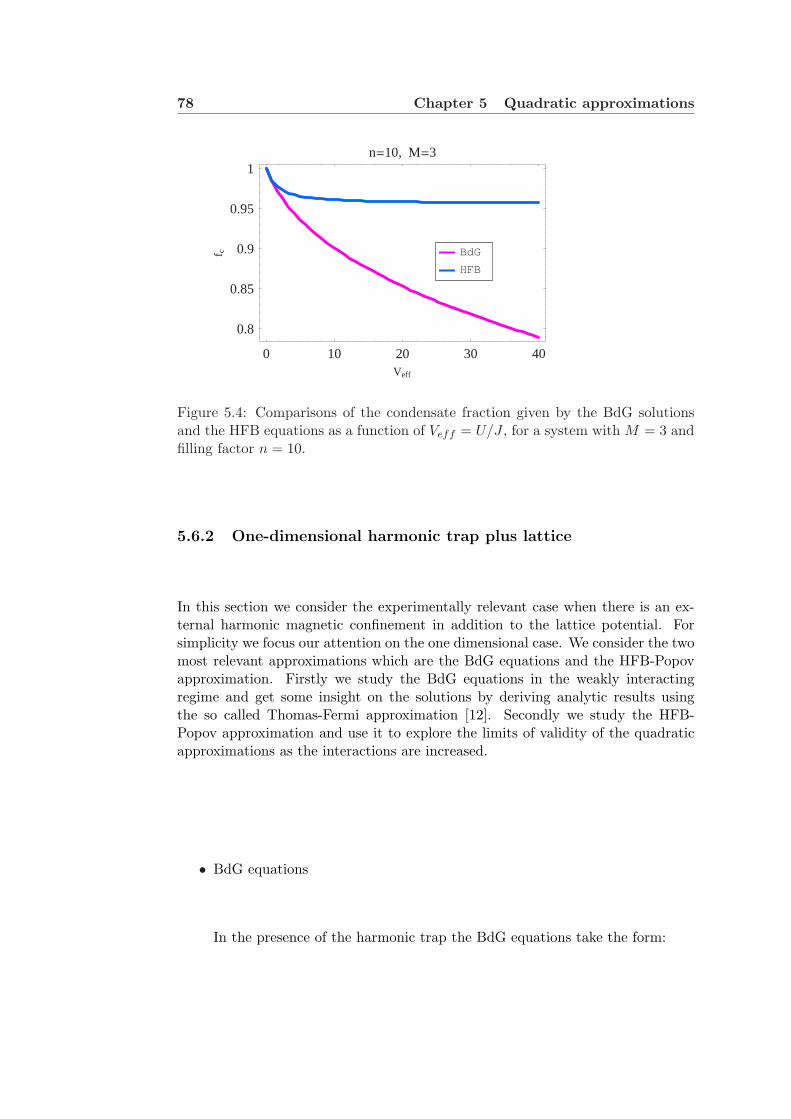
78 Chapter 5 Quadratic approximations
0 10 20 30 40Veff
0.8
0.85
0.9
0.95
1
f c
n=10, M=3
HFB
BdG
Figure 5.4: Comparisons of the condensate fraction given by the BdG solutionsand the HFB equations as a function of Veff = U/J , for a system with M = 3 andfilling factor n = 10.
5.6.2 One-dimensional harmonic trap plus lattice
In this section we consider the experimentally relevant case when there is an ex-ternal harmonic magnetic confinement in addition to the lattice potential. Forsimplicity we focus our attention on the one dimensional case. We consider the twomost relevant approximations which are the BdG equations and the HFB-Popovapproximation. Firstly we study the BdG equations in the weakly interactingregime and get some insight on the solutions by deriving analytic results usingthe so called Thomas-Fermi approximation [12]. Secondly we study the HFB-Popov approximation and use it to explore the limits of validity of the quadraticapproximations as the interactions are increased.
• BdG equations
In the presence of the harmonic trap the BdG equations take the form:

5.6 Applications 79
ωBs us
n + cszn = −J(usn+1 + us
n−1) + (2U |zn|2 − µ + Ωn2)usn
−Uz2nvs
n, (5.94)−ωB
s vsn − csz
∗n = −J(vs
n+1 + vsn−1) + (2U |zn|2 − µ + Ωn2)vs
n
−Uz∗2n usn, (5.95)
µzn = −J(zn+1 + zn−1) + (U |zn|2 + Ωn2)zn, (5.96)
N =∑n
(|zn|2 + nn), (5.97)
nn =∑
s
|vsn|2, (5.98)
cs = U
∑n |zn|2(z∗nus
n − znvsn)∑
n |zn|2 . (5.99)
In the parameter regime where U/J ¿ 1, but the number of atoms is large
enough such that NU/Jaho À 1, where aho=√
m∗ω∗ (See Eq. (2.39)) the
Bogoliubov approximation takes a rather simple analytic form. The effectof increasing the ratio NU/Jaho is to push the atoms outwards, flatteningthe central density and increasing the width of the condensate wavefunction.The quantum pressure, which is proportional to the kinetic energy, takes asignificant contribution only near the edges of the wavefunction, and to agood approximation it can be neglected. This is the so-called Thomas-Fermiapproximation (TF). This approximation has been very useful to derive an-alytic expressions in magnetic confined condensates without the lattice andproved to be in agreement with experimental measurements [12, 18, 19].
Under the Thomas-Fermi approximation one gets a condensate density profileof the form of an inverted parabola which vanishes at the turning pointsRTF =
√µ/Ω:
|zn|2 = µ−Ωn2
U n < RTF
0 n > RTF(5.100)
The chemical potential is determined by fixing the total number of particles.To first order it is possible to neglect the depletion of the condensate andassume that
∑ |zn|2 = N . Changing the sum to an integral it can be solvedfor µ to get
µ = ΩR2TF ,
RTF ≈(
34
NU
Ω
)1/3
. (5.101)

80 Chapter 5 Quadratic approximations
To solve for the excitation spectrum we use the Thomas-Fermi condensateamplitude, Eq.(5.100) into Eqs.(5.94)and (5.95) [18, 111] and use the param-eter J as an expansion parameter in these equations. We define the variablesF q
n = uqn + vq
n and Gsn = us
n − vsn. For simplicity we are going to set the con-
stants cs to zero and ignore the orthogonality constraint at the beginning.We correct this at the end by removing from the modes their projection ontothe condensate. To first order in J we get the following set of equations:
2R2TF Ω
(1− n2
R2TF
)Gs
n = ωBs F s
n, (5.102)
−J
F sn+1 + F s
n−1 − F sn
√1− (n+1)2
R2TF
+√
1− (n−1)2
R2TF√
1− n2
R2TF
= ωBs Gs
n. (5.103)
These two equations can be combined to get a simple equation of the form
√1− (n + 1)2
R2TF
√1− n2
R2TF
(F s
n+1 − F sn
)(5.104)
−√
1− (n− 1)2
R2TF
√1− n2
R2TF
(F s
n−1 − F sn
)= 2
(ωB
s
ω∗
)2
F sn,
with F sn = F s
n/√
1− n2
R2TF
.
The above equation is just the discretized form of the Legendre equation,∂∂x
((1− x2) ∂
∂xPn
)+ n(n + 1)Pn = 0. Therefore the solutions of Eq. (5.104)
are approximately given by :
ωBs = ~ω∗
√s(s + 1)
2, (5.105)
F sn =
√ΩRTF (2s + 1)
ωBs
√1− n2
R2TF
Ps
(n
RTF
), (5.106)
Gsn =
√ωB
s (2s + 1)4ΩR3
TF
1√1− n2
R2TF
Ps
(n
RTF
). (5.107)
The larger the size of the condensate the closer are the approximate solutions,Eq.(5.107), to the exact solutions of Eqs. (5.104).
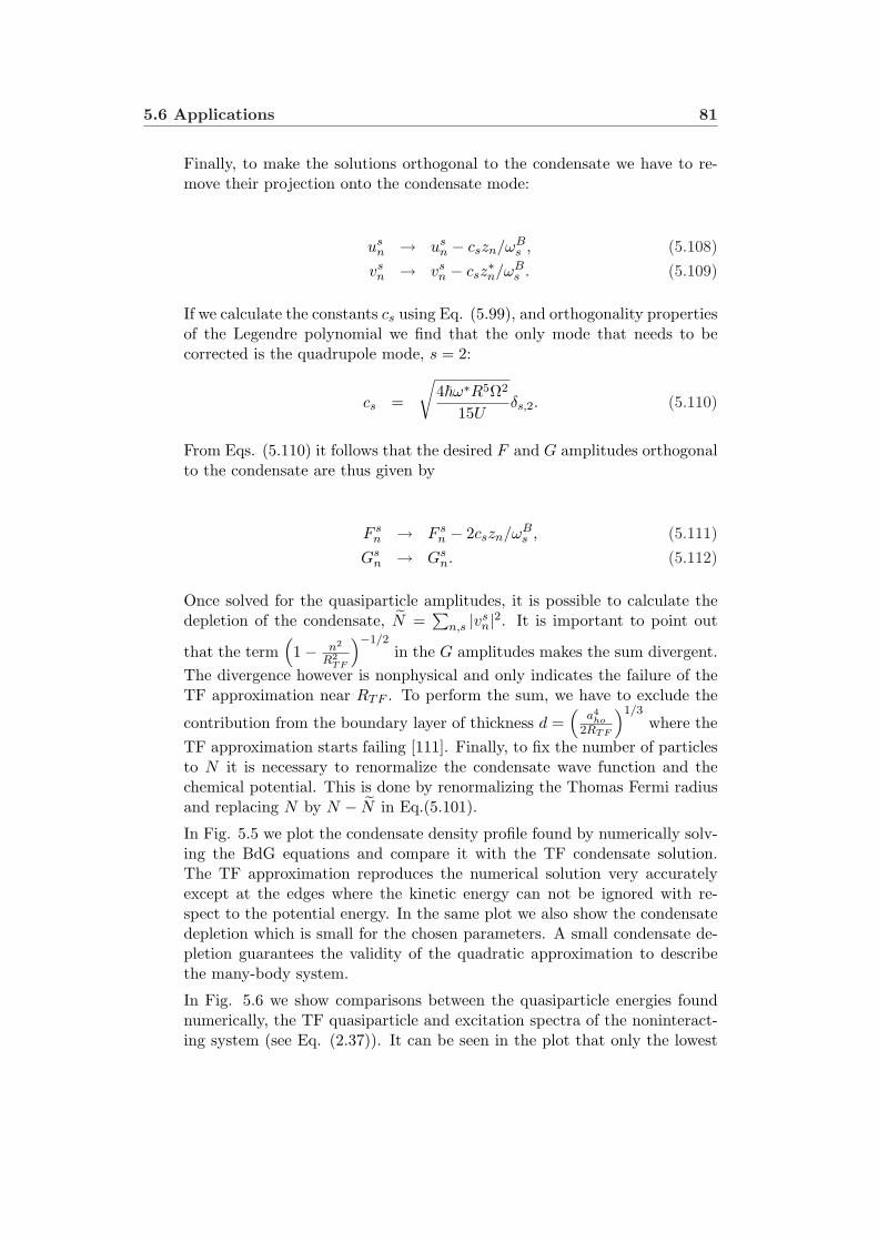
5.6 Applications 81
Finally, to make the solutions orthogonal to the condensate we have to re-move their projection onto the condensate mode:
usn → us
n − cszn/ωBs , (5.108)
vsn → vs
n − csz∗n/ωB
s . (5.109)
If we calculate the constants cs using Eq. (5.99), and orthogonality propertiesof the Legendre polynomial we find that the only mode that needs to becorrected is the quadrupole mode, s = 2:
cs =
√4~ω∗R5Ω2
15Uδs,2. (5.110)
From Eqs. (5.110) it follows that the desired F and G amplitudes orthogonalto the condensate are thus given by
F sn → F s
n − 2cszn/ωBs , (5.111)
Gsn → Gs
n. (5.112)
Once solved for the quasiparticle amplitudes, it is possible to calculate thedepletion of the condensate, N =
∑n,s |vs
n|2. It is important to point out
that the term(1− n2
R2TF
)−1/2in the G amplitudes makes the sum divergent.
The divergence however is nonphysical and only indicates the failure of theTF approximation near RTF . To perform the sum, we have to exclude the
contribution from the boundary layer of thickness d =(
a4ho
2RTF
)1/3where the
TF approximation starts failing [111]. Finally, to fix the number of particlesto N it is necessary to renormalize the condensate wave function and thechemical potential. This is done by renormalizing the Thomas Fermi radiusand replacing N by N − N in Eq.(5.101).
In Fig. 5.5 we plot the condensate density profile found by numerically solv-ing the BdG equations and compare it with the TF condensate solution.The TF approximation reproduces the numerical solution very accuratelyexcept at the edges where the kinetic energy can not be ignored with re-spect to the potential energy. In the same plot we also show the condensatedepletion which is small for the chosen parameters. A small condensate de-pletion guarantees the validity of the quadratic approximation to describethe many-body system.
In Fig. 5.6 we show comparisons between the quasiparticle energies foundnumerically, the TF quasiparticle and excitation spectra of the noninteract-ing system (see Eq. (2.37)). It can be seen in the plot that only the lowest
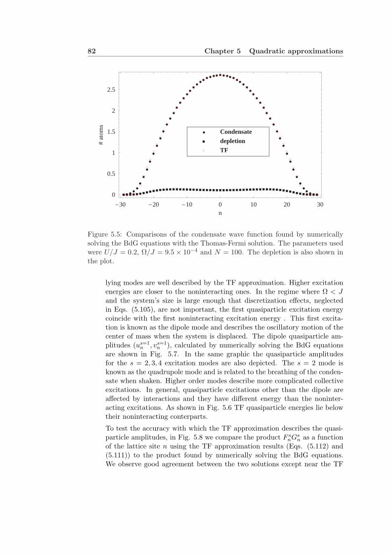
82 Chapter 5 Quadratic approximations
-30 -20 -10 0 10 20 30n
0
0.5
1
1.5
2
2.5
#at
oms
TF
depletion
Condensate
Figure 5.5: Comparisons of the condensate wave function found by numericallysolving the BdG equations with the Thomas-Fermi solution. The parameters usedwere U/J = 0.2, Ω/J = 9.5 × 10⁻⁴ and N = 100. The depletion is also shown inthe plot.
lying modes are well described by the TF approximation. Higher excitationenergies are closer to the noninteracting ones. In the regime where Ω < Jand the system’s size is large enough that discretization effects, neglectedin Eqs. (5.105), are not important, the first quasiparticle excitation energycoincide with the first noninteracting excitation energy . This first excita-tion is known as the dipole mode and describes the oscillatory motion of thecenter of mass when the system is displaced. The dipole quasiparticle am-plitudes (us=1
n , vs=1n ), calculated by numerically solving the BdG equations
are shown in Fig. 5.7. In the same graphic the quasiparticle amplitudesfor the s = 2, 3, 4 excitation modes are also depicted. The s = 2 mode isknown as the quadrupole mode and is related to the breathing of the conden-sate when shaken. Higher order modes describe more complicated collectiveexcitations. In general, quasiparticle excitations other than the dipole areaffected by interactions and they have different energy than the noninter-acting excitations. As shown in Fig. 5.6 TF quasiparticle energies lie belowtheir noninteracting conterparts.
To test the accuracy with which the TF approximation describes the quasi-particle amplitudes, in Fig. 5.8 we compare the product F s
nGsn as a function
of the lattice site n using the TF approximation results (Eqs. (5.112) and(5.111)) to the product found by numerically solving the BdG equations.We observe good agreement between the two solutions except near the TF
5.6 Applications 83
2 4 6 8 10 12 14 16 18 20sth eigenvalue
0.05
0.1
0.15
0.2
0.25Ω
sHE
RL
UJ=0.2 WJ=9.5 x 10⁻⁴ N=100
FreeTFBdG
Figure 5.6: Comparisons of the quasiparticle spectrum found by numerically solv-ing the BdG equations(BdG) with the Thomas-Fermi solution (TF) and the nonin-teracting energies (Free). The parameters used were U/J = 0.2, Ω/J = 9.5×10⁻⁴
and N = 100.
radius. This behavior is consistent with the fact that near the edge of theatomic cloud, the kinetic energy becomes comparable to the potential energyand therefore the TF approximation breaks down.
• HFB-Popov approximation
In the translationally invariant system, both the BdG and the HFB-Popovapproximations give the same quasiparticle amplitudes and energies. How-ever, when the harmonic confinement is present this is no longer the case.The HFB-Popov approximation shifts the quasiparticle energies dependingon the spatial variation of the non condensate density in the region of the con-densate. In this section we investigate the limits of validity of the HFB-Popovapproximation as the parameter U/J is increased. We use the HFB-Popovapproximation instead of the BdG approximation because of the relevantrole of the noncondensate atoms into the condensate as the system is drivento the Mott insulator transition.
In the presence of an harmonic confinement the HFB-Popov equations take
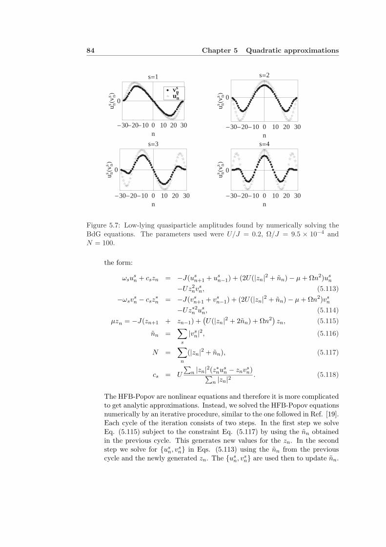
84 Chapter 5 Quadratic approximations
-30-20-10 0 10 20 30n
0
u ns Hv ns L
s=3
-30-20-10 0 10 20 30n
0
u ns Hv ns L
s=4
-30-20-10 0 10 20 30n
0
u ns Hv ns L
s=1
uns
vns
-30-20-10 0 10 20 30n
0
u ns Hv ns L
s=2
Figure 5.7: Low-lying quasiparticle amplitudes found by numerically solving theBdG equations. The parameters used were U/J = 0.2, Ω/J = 9.5 × 10⁻⁴ andN = 100.
the form:
ωsusn + cszn = −J(us
n+1 + usn−1) + (2U(|zn|2 + nn)− µ + Ωn2)us
n
−Uz2nvs
n, (5.113)−ωsv
sn − csz
∗n = −J(vs
n+1 + vsn−1) + (2U(|zn|2 + nn)− µ + Ωn2)vs
n
−Uz∗2n usn, (5.114)
µzn = −J(zn+1 + zn−1) +(U(|zn|2 + 2nn) + Ωn2
)zn, (5.115)
nn =∑
s
|vsn|2, (5.116)
N =∑
n
(|zn|2 + nn), (5.117)
cs = U
∑n |zn|2(z∗nus
n − znvsn)∑
n |zn|2 . (5.118)
The HFB-Popov are nonlinear equations and therefore it is more complicatedto get analytic approximations. Instead, we solved the HFB-Popov equationsnumerically by an iterative procedure, similar to the one followed in Ref. [19].Each cycle of the iteration consists of two steps. In the first step we solveEq. (5.115) subject to the constraint Eq. (5.117) by using the nn obtainedin the previous cycle. This generates new values for the zn. In the secondstep we solve for us
n, vsn in Eqs. (5.113) using the nn from the previous
cycle and the newly generated zn. The usn, vs
n are used then to update nn.
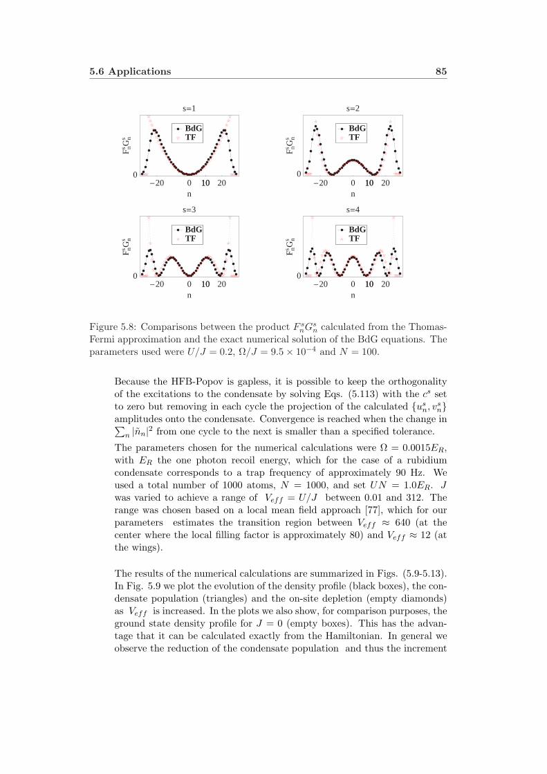
5.6 Applications 85
-20 100 10 20n
0
Fns G
ns
s=3
TFBdG
-20 100 10 20n
0
Fns G
ns
s=4
TFBdG
-20 100 10 20n
0
Fns G
ns
s=1
TFBdG
-20 100 10 20n
0
Fns G
ns
s=2
TFBdG
Figure 5.8: Comparisons between the product F snGs
n calculated from the Thomas-Fermi approximation and the exact numerical solution of the BdG equations. Theparameters used were U/J = 0.2, Ω/J = 9.5× 10⁻⁴ and N = 100.
Because the HFB-Popov is gapless, it is possible to keep the orthogonalityof the excitations to the condensate by solving Eqs. (5.113) with the cs setto zero but removing in each cycle the projection of the calculated us
n, vsn
amplitudes onto the condensate. Convergence is reached when the change in∑n |nn|2 from one cycle to the next is smaller than a specified tolerance.
The parameters chosen for the numerical calculations were Ω = 0.0015ER,with ER the one photon recoil energy, which for the case of a rubidiumcondensate corresponds to a trap frequency of approximately 90 Hz. Weused a total number of 1000 atoms, N = 1000, and set UN = 1.0ER. Jwas varied to achieve a range of Veff = U/J between 0.01 and 312. Therange was chosen based on a local mean field approach [77], which for ourparameters estimates the transition region between Veff ≈ 640 (at thecenter where the local filling factor is approximately 80) and Veff ≈ 12 (atthe wings).
The results of the numerical calculations are summarized in Figs. (5.9-5.13).In Fig. 5.9 we plot the evolution of the density profile (black boxes), the con-densate population (triangles) and the on-site depletion (empty diamonds)as Veff is increased. In the plots we also show, for comparison purposes, theground state density profile for J = 0 (empty boxes). This has the advan-tage that it can be calculated exactly from the Hamiltonian. In general weobserve the reduction of the condensate population and thus the increment

86 Chapter 5 Quadratic approximations
Veff=100
-10 -5 0 5 10i
20
40
60
80 Veff=312
-10 -5 0 5 10i
20
40
60
80
Veff=3
20
40
60
80 Veff=11
20
40
60
80
Veff=0.01
20
40
60
80 Veff=0.09
20
40
60
80
Figure 5.9: Condensate density (triangles), total density (filled boxes) and localdepletion (empty diamonds) as a function of the lattice site i for different valuesof Veff..The site indices i are chosen such that i = 0 corresponds to the center ofthe trap. Although these quantities are defined only at the discrete lattice siteswe join them to help visualization. The empty boxes represent the exact solutionfor the case J=0.
of the depletion with increasing interaction strength. When the system is inthe superfluid regime, most of the atoms are in the condensate, but as J isdecreased the depletion of the condensate becomes very important.
For the chosen parameters, the density profile has a parabolic shape reflectingthe confining potential. By comparing the evolution of the density as J isdecreased with the exact solution at J = 0, we can crudely estimate thevalidity of the HFB-Popov calculations. The density evolves from a Gaussiantype (see plots for Veff = 0.01 and 0.09) with smooth edges towards aThomas-Fermi profile with sharp edges adjusting its shape to the J = 0profile. We can appreciate that around Veff = 3 both profiles are almostequal. For lower values of J the HFB-Popov density starts to differ fromthe J = 0 limit, even though the system is closer to the J = 0 limit. Wecan say that beyond this point higher order correlations, neglected by thetheory, begin to be important. The departure of the HFB-Popov densityprofile from the J = 0 one as J is decreased begins at the edges (see thepanels corresponding to Veff = 11 and 100). This is expected if we considerthe on-site depletion. For such values of Veff the local depletion in the wings
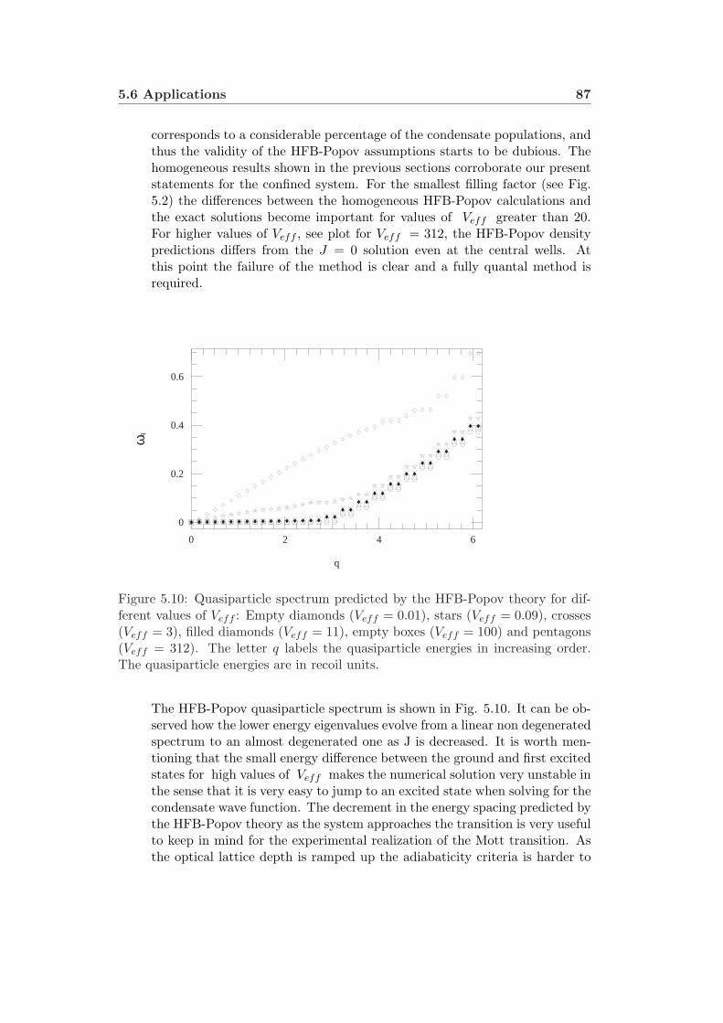
5.6 Applications 87
corresponds to a considerable percentage of the condensate populations, andthus the validity of the HFB-Popov assumptions starts to be dubious. Thehomogeneous results shown in the previous sections corroborate our presentstatements for the confined system. For the smallest filling factor (see Fig.5.2) the differences between the homogeneous HFB-Popov calculations andthe exact solutions become important for values of Veff greater than 20.For higher values of Veff , see plot for Veff = 312, the HFB-Popov densitypredictions differs from the J = 0 solution even at the central wells. Atthis point the failure of the method is clear and a fully quantal method isrequired.
0 2 4 6
q
0
0.2
0.4
0.6
ωq
Figure 5.10: Quasiparticle spectrum predicted by the HFB-Popov theory for dif-ferent values of Veff : Empty diamonds (Veff = 0.01), stars (Veff = 0.09), crosses(Veff = 3), filled diamonds (Veff = 11), empty boxes (Veff = 100) and pentagons(Veff = 312). The letter q labels the quasiparticle energies in increasing order.The quasiparticle energies are in recoil units.
The HFB-Popov quasiparticle spectrum is shown in Fig. 5.10. It can be ob-served how the lower energy eigenvalues evolve from a linear non degeneratedspectrum to an almost degenerated one as J is decreased. It is worth men-tioning that the small energy difference between the ground and first excitedstates for high values of Veff makes the numerical solution very unstable inthe sense that it is very easy to jump to an excited state when solving for thecondensate wave function. The decrement in the energy spacing predicted bythe HFB-Popov theory as the system approaches the transition is very usefulto keep in mind for the experimental realization of the Mott transition. Asthe optical lattice depth is ramped up the adiabaticity criteria is harder to
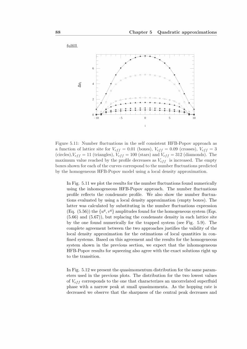
88 Chapter 5 Quadratic approximations
fulfill.
-10 -5 0 5 10
i
0
2
4
6
∆ni
Figure 5.11: Number fluctuations in the self consistent HFB-Popov approach asa function of lattice site for Veff = 0.01 (boxes), Veff = 0.09 (crosses), Veff = 3(circles),Veff = 11 (triangles), Veff = 100 (stars) and Veff = 312 (diamonds). Themaximum value reached by the profile decreases as Veff is increased. The emptyboxes shown for each of the curves correspond to the number fluctuations predictedby the homogeneous HFB-Popov model using a local density approximation.
In Fig. 5.11 we plot the results for the number fluctuations found numericallyusing the inhomogeneous HFB-Popov approach. The number fluctuationsprofile reflects the condensate profile. We also show the number fluctua-tions evaluated by using a local density approximation (empty boxes). Thelatter was calculated by substituting in the number fluctuations expression(Eq. (5.56)) the uq, vq amplitudes found for the homogeneous system (Eqs.(5.66) and (5.67)), but replacing the condensate density in each lattice siteby the one found numerically for the trapped system (see Fig. 5.9). Thecomplete agreement between the two approaches justifies the validity of thelocal density approximation for the estimations of local quantities in con-fined systems. Based on this agreement and the results for the homogeneoussystem shown in the previous section, we expect that the inhomogeneousHFB-Popov results for squeezing also agree with the exact solutions right upto the transition.
In Fig. 5.12 we present the quasimomentum distribution for the same param-eters used in the previous plots. The distribution for the two lowest valuesof Veff corresponds to the one that characterizes an uncorrelated superfluidphase with a narrow peak at small quasimomenta. As the hopping rate isdecreased we observe that the sharpness of the central peak decreases and

5.6 Applications 89
Veff=100
0 1 2 3aq
0
100
200
n q
Veff=312
0 1 2 3aq
Veff=3
0
100
200
300
n q Veff=11
Veff=0.01
0
100
200
300
400
n q Veff=0.09
Figure 5.12: Quasimomentum distribution as a function of qa, a the lattice spacing,q the quasimomentum, for different values of Veff .
the distribution extends towards large quasi-momenta. It is interesting tonote the appearance of a small peak between q = 0.5 and 1 which is mostnoticeable for the Veff = 3 case. This agrees with numerical solutions ofthe Bose-Hubbard Hamiltonian using Monte Carlo simulations [112]. Weattribute the origin of the small peak to the depletion of the condensate atthe wings. For the parameters when the small peak is present, the mostimportant contribution to the quasimomentum distribution still comes fromthe condensate atoms. The step function like shape of the condensate profilecauses an oscillatory | sin(x)/x| shape of the quasimomentum distribution.As the lattice depth is increased the hopping becomes energetically costly,the long-range order starts to decrease and the Fourier spectrum becomesbroader.
In Fig. 5.13 we plot the first order on site superfluid fraction f(1)sn which was
defined in Eq.(5.60). The curves corresponding to Veff = 0.01 − 11, whichare in the regime where the HFB-Popov is expected to be valid, depicthow as Veff is increased the superfluid profile decreases faster at the wingsand at the center but no major change is observed in the middle section.The evolution of the on-site superfluidity as the interaction strength is in-

90 Chapter 5 Quadratic approximations
-10 -5 0 5 10
i
0
0.02
0.04
0.06
0.08
0.1
f sc(
1)
Figure 5.13: First order on-site superfluid fraction as a function of the lattice site ifor different values of Veff ..The site indices i are chosen such that i = 0 correspondsto the center of the trap. Filled boxes: Veff . =0.01, empty boxes: Veff . = 0.09,empty diamonds: Veff . = 3, stars: Veff . = 11, crosses: Veff . = 100 and triangles:Veff . = 312.
creased, exhibiting a domain localized decrement instead of a global one, isin agreement with the development of uncompressible regions surroundedby superfluid rings predicted for trapped systems [79] as the transition isapproached.
The Mott transition is a quantum phase transition and as for all critical phe-nomena, its behavior depends strongly on the dimensionality of the system.In the present analysis, due to computational limitations, we considered onedimensional systems. Experimentally, the Mott transition has been achieved[46] in a 3 dimensional lattice with filling factors between 1 and 3. Eventhough the HFB-Popov approach fails to describe the strong coupling regimefor the one dimensional systems we considered, we showed how the methodis incredibly powerful in describing most of its characteristic features as theyare driven from the superfluid regime towards the transition. We expectthe HFB-Popov method to give a better description of the transition as thedimensionality of the system is increased and therefore to be a good modelin an experimental situation.
As shown in previous studies [44], [79] the Mott transition in a d-dimensionalhomogeneous system has two different critical behaviors: one (d+1) XY- like,for systems with fixed integer density as the interaction strength is changed,and one mean field-like exhibited when the transition is induced by changing
5.7 Improved HFB-Popov approximation 91
the density. Different from the homogeneous case where the Mott transitionis characterized by the global offset of the superfluidity, for confined systems,commensuration is only well defined locally. The inhomogeneity introducedby the confining potential allows the existence of extended Mott domains(above a critical interaction strength) surrounded by superfluid ones [79],thus the total superfluid fraction doesn’t vanishes in the Mott regime. Thisissue, together with the fact that the finite length scale introduced by the trapsuppresses the long wave fluctuations which are responsible for destroying themean field [16]1, make us believe the critical behavior in confined systems tobe more mean-field like. Because the critical dimension for the latter typeof transition is two [44], [79], we expect that for trapped systems in d = 3,the range of validity of the HFB-Popov extends closer to the transition.
5.7 Improved HFB-Popov approximation
The corrections to the quadratic Hamiltonian from higher order terms have essen-tially two major effects. Firstly, they include the effect of the interactions betweencondensate and noncondensate atoms on the behavior of the condensate. Secondly,they take into account the effect of the surrounding atoms on the nature of theinteratomic collisions. We mentioned previously that although the HFB treatmentshould represent an advance over the BdG theory it is not useful in practice be-cause it is not gapless. In the first part of this section we show, how, by takinginto account the anomalous average m (Eq. (5.18)) we actually upgrade the bareinteraction potential U to the many body scattering matrix which gives a betterdescription of interparticle collisions. The problem with the HFB equations is thatnot all the interactions are upgraded and the diagonal elements still contain bareinteraction terms. The different treatment of the off diagonal and diagonal termsis caused by the factorization approximation on which the HFB approximation isbased. The factorization is appropriate for the quartic term in the Hamiltonian(as it is justified by Wick’s theorem [16]) but not for the cubic terms.
To solve the problem the first approximation that one might think of is toupgrade by hand the bare interactions in the diagonal terms and replace themby the many-body scattering matrix. This procedure is known as the improvedPopov approximation [53, 16]. In this section, we discuss the improved Popovapproximation and apply it to a translationally invariant system. We explicitlyshow that the improved Popov approximation gives a better description of themany-body physics as the Mott insulator transition is approached in comparisonwith the regular HFB-Popov approximation.
1One obvious consequence of this is that BEC is possible in one and two dimensions in a trapwhereas in the homogeneous, thermodynamic limit it can not occur in fewer than three dimensions
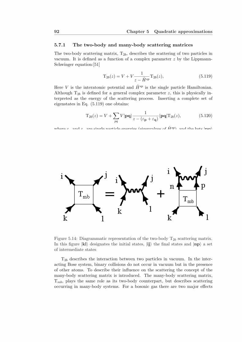
92 Chapter 5 Quadratic approximations
5.7.1 The two-body and many-body scattering matrices
The two-body scattering matrix, T2b, describes the scattering of two particles invacuum. It is defined as a function of a complex parameter z by the Lippmann-Schwinger equation:[51]
T2b(z) = V + V1
z − HspT2b(z), (5.119)
Here V is the interatomic potential and Hsp is the single particle Hamiltonian.Although T2b is defined for a general complex parameter z, this is physically in-terpreted as the energy of the scattering process. Inserting a complete set ofeigenstates in Eq. (5.119) one obtains:
T2b(z) = V +∑pq
V |pq〉 1z − (εp + εq)
〈pq|T2b(z), (5.120)
where εp and εq are single particle energies (eigenvalues of Hsp), and the kets |pq〉are the corresponding two particle eigenstates and describe the intermediate statesin the collision of two atoms. A diagrammatic representation of T2b is shown inFig. 5.14. Because of the ladder shape of the diagrams included in the scatteringmatrix, they are usually referred as ladder diagrams.
Figure 5.14: Diagrammatic representation of the two-body T2b scattering matrix.In this figure |kl〉 designates the initial states, |ij〉 the final states and |np〉 a setof intermediate states
T2b describes the interaction between two particles in vacuum. In the inter-acting Bose system, binary collisions do not occur in vacuum but in the presenceof other atoms. To describe their influence on the scattering the concept of themany-body scattering matrix is introduced. The many-body scattering matrix,Tmb, plays the same role as its two-body counterpart, but describes scatteringoccurring in many-body systems. For a bosonic gas there are two major effects
5.7 Improved HFB-Popov approximation 93
which need to be accounted for as compared to scattering in vacuum. First of all,the relevant states which enter in the matrix elements should be many-body statesrather than single particle ones. Second, Tmb should account for Bose enhance-ment of a scattering process. Various forms for the Tmb have been been proposedin the literature [16, 53, 54, 113] depending upon the approximations made. Theone that we are going to use is a simplest generalization of the two-body matrixgiven by [16, 113]:
Tmb(z) = V +∑pq
V |pq〉 1 + np + nq
z − (ωp + ωq)〈pq|Tmb(z), (5.121)
where z is again a complex parameter, ωp and ωq are quasiparticle energies, nq
and np are thermal quasiparticle occupation factors which vanish at T = 0, and|pq〉 correspond to single-particle wave functions. The full quasiparticle characterof the intermediate states is not taken into account in this simple definition. Amore general many-body scattering matrix which includes the full quasiparticlewave functions has been discussed by Bijlsma and Stoof [53]. However this simplerTmb matrix is the one that naturally appears in the many-body theory, at least atlowest order.
At this point it is important to highlight that the zero energy of the many-bodyscattering matrix is not the same as the zero energy in its two-body counterpart.Because the two-body matrix is written in terms of single particle energies, inthis case the z is measured relative to the energy of a stationary particle. In themany-body case Tmb is defined in terms of quasiparticle energies and therefore zis measured with respect to the condensate chemical potential. In the dilute gaslimit, where the inter-particle distance is large compared with the s-wave scatteringlength, the ladder diagrams included in the Tmb give the largest contribution tothe modification of the bare potential due to interactions.
5.7.2 The anomalous average and the many-body scattering ma-trix
In this section we are going to follow [16, 53] to show how by including the anoma-lous average the many-body scattering matrix is introduced into the theory. Forinterpretation purposes we are going to restrict the analysis to the translationallyinvariant system.
The anomalous average m is defined in terms of the quasiparticle amplitudesuq and vq according to Eq.(5.93). The product uqvq, on the other hand, is relatedto the off diagonal matrix elements, see Eq.(5.90). If we combine the two equationswe get an expression for the off diagonal matrix element Mq−q given by
Mq−q
no= U +
U
M
∑p
1−(ωp + ω−p)
Mq−q
no. (5.122)
To make the connection with the many-body scattering matrix, let us take theinner product of Eq. (5.121), with the states 〈q− q| and |00〉 and evaluate it at
94 Chapter 5 Quadratic approximations
z = 0. At zero temperature, the thermal occupation factors vanish, nq = 0 and weget:
〈q− q|Tmb(0)|00〉 = 〈q− q|V |00〉+∑
pk
〈q− q|V |pk〉 1−(ωp + ωk)
〈pk|Tmb(0)|00〉.
(5.123)The quantity 〈k1k2|V |k3k4〉 is the momentum representation of the two-body
interaction potential V . In the Bose-Hubbard Hamiltonian we assume a contactpotential with amplitude U which yields a potential in the momentum represen-tation given by
〈k1k2|V |k3k4〉 =U
Mδk1+k2,k3+k4 . (5.124)
Using Eq. (5.124) into (Eq. 5.123) we obtain
Tmb = U +1M
∑p
U1
−(ωp + ω−p)Tmb, (5.125)
with
〈p− p|Tmb(0)|00〉 ≡ 1MTmb. (5.126)
Eqs. (5.125) and (5.122) imply that Mq−q = noTmb, and therefore that by includ-ing the anomalous average in the equations, the off diagonal matrix element givenby Uno in the BdG equations is upgraded to Tmbno in the HFB equations.
The many-body scattering matrix also appears in the DNLSE since Eq. (5.89)contains m:
µ = −tJ + Uno + 2Un + Um = −tJ + Tmbno + 2Un. (5.127)
Finally, to conclude this section we just rewrite the HFB equations in terms ofTmb obtaining:
(εq + no(2U − Tmb) −noTmb
noTmb −εq − no(2U − Tmb)
)(uq
vq
)= ωq
(uq
vq
). (5.128)
This allow us to explicitly see the different treatment that the theory gives to thediagonal and off diagonal terms: The bare potential is completely upgraded toTmb in the off diagonal terms but is not in the diagonal ones, and in the chemicalpotential.

5.7 Improved HFB-Popov approximation 95
5.7.3 Improved Popov approximation
The appearance of a gap in the HFB equations is because of the different treatmentof the off diagonal and diagonal terms. We will show in chapter 8 that as wego beyond the quadratic approximation of the Hamiltonian and include higherorder corrections we start to incorporate the many-body scattering in the diagonalterms. However, a naive way to correct for the gap problem in the HFB equationsis simple to upgrade by hand the interactions in the diagonal terms and replacethem by the many-body scattering matrix. This way to proceed is known as theimproved Popov approximation [16, 53]. The matrix we have to diagonalize underthe improved Popov approximation is:
(εq + noTmb −noTmb
noTmb −(εq + noTmb)
)(uq
vq
)= ωq
(uq
vq
)(5.129)
µ = −tJ + Tmbno + 2Tmbn (5.130)
Eqs. (5.129) and (5.130) together with Eq. (5.125) and Eq. (5.69) form a closedset of equations. They are exactly the same than the HFB-Popov equations ifU is replaced by Tmb. The reason why there are two different coupling constantin the equation for the chemical potential Tmb and Tmb, is because they describetwo different scattering processes. The second term in the right hand side of Eq.(5.130) describes the scattering between two atoms in the condensate colliding atzero momentum, 〈q− q|Tmb(0)|00〉, and that is why the coupling constant is Tmb
(see Eq. 5.126). On the other hand, the third term describes the collision betweenone condensate atom and one atom out of the condensate and the coupling constantin this case should be evaluated at different energy Tmb ∝
∑p〈p0|Tmb(ωp)|0p〉.
The extra difficulty that the improved Popov equations have compare with theHFB-Popov equations is that Tmb depends on the quasiparticle energies and allequations must be solved in a self consistent way. To get simple analytic expressionswe start by analyzing limiting regimes.
• Case noTmb > J
In this regime the quasiparticle energy can be approximated by ωq v√
2noTmbεq.Using this approximation in the expression for the many-body scattering ma-trix we obtain
Tmb =U
1 +√
U2α2
noJTmb
, (5.131)
with α defined in Eq. (5.73). Solving the algebraic equation we get twopossible solutions
Tmb = U ± U2
2Jno
(α2 +
√α4 +
4Jnoα2
U
). (5.132)

96 Chapter 5 Quadratic approximations
Because we want the root which increases as U increases we choose thesolution with positive sign.
• Case noTmb < J
In general one can show that the condition noTmb < J is only satisfied if thequantity Tmb/J is small. This also implies that the parameter U/J must besmall. In this regime, therefore, we can perturbativelly expand Eq.( 5.131 )in powers of U/J to get:
Tmb v U
(1 + O
(U
J
)). (5.133)
The fact that Eq. (5.134) has the correct asymptotic behavior in the limit noTmb <J (it approaches to U as U goes to zero) even though it was derived under theassumption noTmb > J , allow us to extend the validity of Eq. (5.132) to all regimes.Therefore, to a good approximation, we get a general formula for Tmb given by:
Tmb = U +U2
2Jno
(α2 +
√α4 +
4Jnoα2
U
). (5.134)
We have checked numerically that in fact, Eq. (5.134) is a very good approximationof Tmb in all regimes.Having an analytic expression for Tmb, we can solve for the condensate density toget:
no = n− 1M
∑
q 6=0
εq + Uno
2ωq+
12,
≈ g − α
√Tmb
Jno. (5.135)
In the above equation we used the same approximations that lead to Eq.(5.72),which was explicitly showed to be good in Figs. 5.2 and 5.3 and the definition ofg given in Eq. (5.74).
If we solve Eq. (5.135), we finally obtain an analytic expression for no
no ≈ g − α
√Ug
J. (5.136)
Surprisingly, the expression for the condensate density that we get after includingthe many-body scattering matrix is exactly the same, as the one we get if in theBdG equations for the condensate, Eq. (5.72), we replace no by g in the righthand side. Except for the term M−1
2M , this corresponds to the lowest order solutionwe can get of Eq. (5.72), where instead of solving self consistently the algebraicequation we replace no by n. The term M−1
2M is very small at high densities whenn + 1/2 ≈ n, regime where in fact we only expect a mean field treatment to bevalid and it might be interpreted as a finite size effect. Hereafter we are going
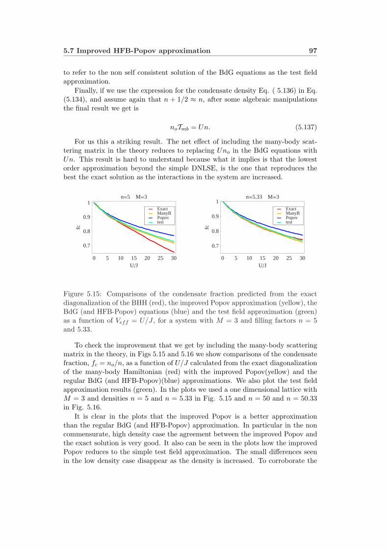
5.7 Improved HFB-Popov approximation 97
to refer to the non self consistent solution of the BdG equations as the test fieldapproximation.
Finally, if we use the expression for the condensate density Eq. ( 5.136) in Eq.(5.134), and assume again that n + 1/2 ≈ n, after some algebraic manipulationsthe final result we get is
noTmb = Un. (5.137)
For us this a striking result. The net effect of including the many-body scat-tering matrix in the theory reduces to replacing Uno in the BdG equations withUn. This result is hard to understand because what it implies is that the lowestorder approximation beyond the simple DNLSE, is the one that reproduces thebest the exact solution as the interactions in the system are increased.
0 5 10 15 20 25 30UJ
0.7
0.8
0.9
1
fc
n=5 M=3
testPopovManyBExact
0 5 10 15 20 25 30UJ
0.7
0.8
0.9
1fc
n=5.33 M=3
testPopovManyBExact
Figure 5.15: Comparisons of the condensate fraction predicted from the exactdiagonalization of the BHH (red), the improved Popov approximation (yellow), theBdG (and HFB-Popov) equations (blue) and the test field approximation (green)as a function of Veff = U/J , for a system with M = 3 and filling factors n = 5and 5.33.
To check the improvement that we get by including the many-body scatteringmatrix in the theory, in Figs 5.15 and 5.16 we show comparisons of the condensatefraction, fc = no/n, as a function of U/J calculated from the exact diagonalizationof the many-body Hamiltonian (red) with the improved Popov(yellow) and theregular BdG (and HFB-Popov)(blue) approximations. We also plot the test fieldapproximation results (green). In the plots we used a one dimensional lattice withM = 3 and densities n = 5 and n = 5.33 in Fig. 5.15 and n = 50 and n = 50.33in Fig. 5.16.
It is clear in the plots that the improved Popov is a better approximationthan the regular BdG (and HFB-Popov) approximation. In particular in the noncommensurate, high density case the agreement between the improved Popov andthe exact solution is very good. It also can be seen in the plots how the improvedPopov reduces to the simple test field approximation. The small differences seenin the low density case disappear as the density is increased. To corroborate the
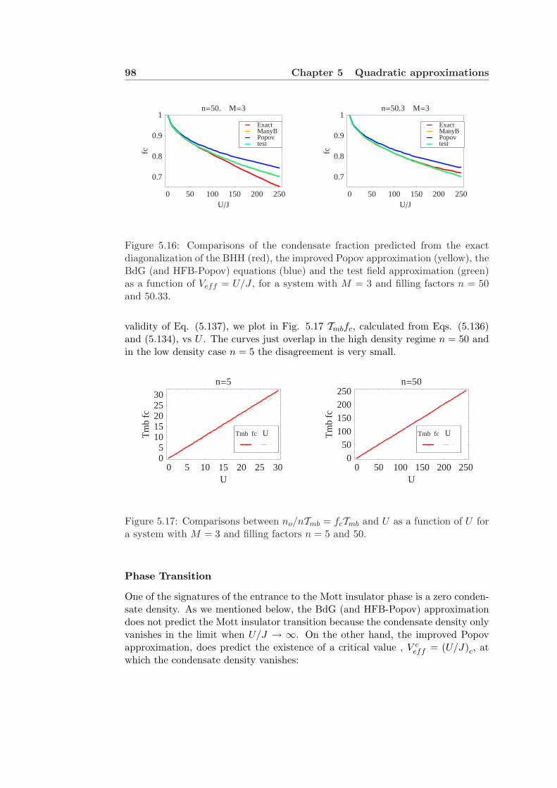
98 Chapter 5 Quadratic approximations
0 50 100 150 200 250UJ
0.7
0.8
0.9
1
fc
n=50. M=3
testPopovManyBExact
0 50 100 150 200 250UJ
0.7
0.8
0.9
1
fc
n=50.3 M=3
testPopovManyBExact
Figure 5.16: Comparisons of the condensate fraction predicted from the exactdiagonalization of the BHH (red), the improved Popov approximation (yellow), theBdG (and HFB-Popov) equations (blue) and the test field approximation (green)as a function of Veff = U/J , for a system with M = 3 and filling factors n = 50and 50.33.
validity of Eq. (5.137), we plot in Fig. 5.17 Tmbfc, calculated from Eqs. (5.136)and (5.134), vs U . The curves just overlap in the high density regime n = 50 andin the low density case n = 5 the disagreement is very small.
0 5 10 15 20 25 30U
05
1015202530
Tm
bfc
n=5
Tmb fc U
0 50 100 150 200 250U
0
50
100
150
200
250
Tm
bfc
n=50
Tmb fc U
Figure 5.17: Comparisons between no/nTmb = fcTmb and U as a function of U fora system with M = 3 and filling factors n = 5 and 50.
Phase Transition
One of the signatures of the entrance to the Mott insulator phase is a zero conden-sate density. As we mentioned below, the BdG (and HFB-Popov) approximationdoes not predict the Mott insulator transition because the condensate density onlyvanishes in the limit when U/J → ∞. On the other hand, the improved Popovapproximation, does predict the existence of a critical value , V c
eff = (U/J)c, atwhich the condensate density vanishes:
5.8 Conclusions 99
V ceff =
n + M−12M
α2−−→nÀ1
n
α2. (5.138)
If we compare the above expression with the equation of the critical point calcu-lated from a mean field model starting in the Mott insulator phase (see chapter 3)given by, V c
eff = t((2n + 1) +
(√(2n + 1)2 − 1
)), we see that in the high density
limit, the only regime where mean field theories are expected to be valid, bothequations describe a critical point which scales linear with n and with a propor-tionality constant which depends only on the dimensionality of the system. In theimproved Popov approximation the proportionality constant is 1/α2, in the meanfield theory starting from the Mott phase it is 8t (remember t is the number ofnearest neighbors). For a one dimensional lattice in the thermodynamic limit theimproved Popov approximation has the infrared divergency problem, α →∞ andthe critical point approaches zero. However, this is consistent with the calculationsdone in Ref. [44] where the authors showed using renormalization group techniquesthat the upper critical dimension for the transition at constant integer density isdc = 2.
Nevertheless, the phase transition predicted by the improved Popov approxi-mation does not have a clear connection to the real Mott insulator phase transition.A specific problem is the fact that the improved Popov approximation does not dis-tinguish between commensurate and incommensurate fillings. This distinction iscrucial to reproduce the characteristic superfluid to Mott insulator phase diagram.Furthermore, there is not clear signature that the system becomes incompress-ible in the Mott phase, and no gap in the excitation spectrum opens up as thetransition is reached.
5.8 Conclusions
In summary, in this chapter we have developed quadratic approximations for de-scribing the approach of a superfluid system towards the Mott insulator transition.We have shown that this method can be used to predict the relevant physical quan-tities over a useful range. However, the quadratic approximations are developedassuming small fluctuations and therefore as soon as quantum correlations becomeimportant it is clear that a fully quantal method is required.

100 Chapter 5 Quadratic approximations
Chapter 6
The two particle irreducibleeffective action (2PI) and theclosed time path (CTP)formalism
In the last section we focused our attention on quadratic approximations of themany body Hamiltonian and we used them to describe equilibrium properties ofultra cold atoms loaded in optical lattices. In this chapter extend our analysis tonon equilibrium systems. The description of the evolution of condensates far fromequilibrium has gained considerable importance in matter-wave physics, motivatedby recent experimental achievements such as the colliding and collapsing conden-sates [20, 21, 115, 114], collapses and revivals of the coherent matter field [47]and the NIST patterned loading experiment described in chapter 4. To date mosttheoretical descriptions of nonequilibrium dynamics of BEC’s have been based onthe time dependent Gross-Pitaevskii equation, coupled with extended kinetic theo-ries that describe excitations in dilute weakly interacting systems close to thermalequilibrium ([15],[58]-[62],[116]). However, experiments such as those mentionedabove have been able to achieve regimes where the standard mean field descriptionis inapplicable, so new methods are required.
To treat far-from-equilibrium dynamics, in this chapter we adopt a closed timepath (CTP) [56] functional-integral formalism together with a two-particle irre-ducible (2PI) [57] effective action approach. We retain terms of up to second-orderin the interaction strength when solving these equations. This method has beengeneralized for and applied to the establishment of a quantum kinetic field the-ory [117, 118, 119] with applications to problems in gravitation and cosmology[120, 121], particles and fields [122, 123], BEC [54, 125] and condensed matter sys-tems [124] as well as addressing the issues of thermalization and quantum phasetransitions [126, 127, 128].
In this chapter we consider under the 2PI-CTP scheme different approxima-tions: the Hartree-Fock-Bogoliubov (HFB) approximation, the next-to-leading

102Chapter 6 The two particle irreducible effective action (2PI) and the
closed time path (CTP) formalism
order 1/N expansion of the 2PI effective action up to second-order in the in-teraction strength and a second-order perturbative expansion in the interactionstrength. In chapter 7 we apply the 2PI-CTP approximations derived here to de-scribe the the patterned loading experiment [33] previously discussed in chapter4.
6.1 2PI effective action Γ(z, G)
Figure 6.1: Two-loop (upper row) and three-loop diagrams (lower row) contribut-ing to the effective action. Explicitly, the diagram a) is what we call the double-bubble , b) the setting-sun and c) the basketball.
The first requirement for the study of nonequilibrium processes is a generalinitial-value formulation depicting the dynamics of interacting quantum fields. TheCTP or Schwinger-Keldysh effective action formalism [56] serves this purpose. Thesecond requirement is to describe the evolution of the correlation functions andthe mean field on an equal footing. The two particle irreducible (2PI) formalism[57] where the correlation functions appear also as independent variables, servesthis purpose. By requiring the generalized (master) CTP effective action [118] tobe stationary with respect to variations of the correlation functions we obtain aninfinite set of coupled (Schwinger-Dyson) equations for the correlation functionswhich is a quantum analog of the BBGKY hierarchy. The 2PI effective actionproduces two such functions in this hierarchy. In this section we shall focus on the2PI formalism, and then upgrade it to the CTP version in the next section.
Our starting point is the one dimensional Bose-Hubbard Hamiltonian (see chap-ter 3).
H = −J∑
i
(a†i ai+1 + a†i+1 ai ) +12U
∑
i
a†i a†i ai ai +∑
i
Via†i ai (6.1)

6.1 2PI effective action Γ(z, G) 103
where ai and a†i are the bosonic operators that annihilate and create an atomon the site i. Here, the parameter U denotes the strength of the on-site repulsionof two atoms on the site i; the parameter Vi denotes the energy offset of eachlattice site due to an additional slowly- varying external potential that might bepresent (such as a magnetic trap), and J denotes the hopping rate between adjacentsites. Because the next-to-nearest neighbor amplitudes are typically two orders ofmagnitude smaller, tunneling to next-to-nearest neighbor sites can be neglected.The Bose -Hubbard Hamiltonian should be an appropriate model when the loadingprocess produces atoms in the lowest vibrational state of each well, with a chemicalpotential smaller than the distance of the first vibrationally excited state.
Hereafter we consider for simplicity only a homogeneous lattice with periodicboundary conditions and no other external potential (Vi = 0). Once the equationsof motion are derived, it is straightforward to generalize them to higher dimensionsor to include additional external potentials. As usual, we denote the total numberof atoms by N and the number of lattice sites by M .
The classical action associated with the Bose-Hubbard Hamiltonian (6.1), isgiven in terms of the complex fields ai and a∗i by
S[a∗i , ai] =∫
dt∑
i
i~a∗i (t)∂tai(t)
+∫
dt∑
i
J(a∗i (t)ai+1(t) + ai(t)a∗i+1(t)
)(6.2)
−∫
dt∑
i
U
2a∗i (t)a
∗i (t)ai(t)ai(t).
To simplify our notation we introduce aai (a = 1, 2) defined by
ai = a1i , a∗i = a2
i . (6.3)
In terms of these fields the classical action takes the form
S[a] =∫
dt∑
i
12haba
ai (t)~∂ta
bi(t (6.4)
+∫
dt∑
i
(Jσaba
ai+1(t)a
bi(t)−
U
4N (σabaai (t)a
bi(t))
2
),
where N is the number of fields,which is two in this case, and summation overrepeated field indices a, b = (1, 2) is implied and hab and σab are matrices definedas
hab = i
(0 −11 0
), σab =
(0 11 0
). (6.5)
In terms of the familiar Pauli matrices, σab = σx and hab = −σy.

104Chapter 6 The two particle irreducible effective action (2PI) and the
closed time path (CTP) formalism
After second quantization the fields aai are promoted to operators. We denote
the expectation value of the field operator, i.e. the mean field, by zai (t) and the
expectation value of the composite field by Gabij (t, t′). Physically, |za
i (t)|2 is thecondensate population and the composite fields determine the fluctuations aroundthe mean field:
zai (t) = 〈aa
i (t)〉 , (6.6)
Gabij (t, t′) =
⟨TCaa
i (t)abi(t
′)⟩− 〈aa
i (t)〉⟨ab
i(t′)⟩
. (6.7)
The brackets denote the expectation value with respect to the density matrix andTC denotes time ordering along a contour C in the complex plane.
All correlation functions of the quantum theory can be obtained from the effec-tive action Γ[z,G], the two particle irreducible generating functional for Green’sfunctions parameterized by za
i (t) and the composite field Gabij (t, t′). To get an
expression for the effective action we first define the functional Z[J,K] [57] as
Z[J,K] = eiW [J,K]/~ (6.8)
=∏a
∫Daa exp
i
~
S[a] +
∫dt
∑
i
Jia(t)aai (t) +
12
∫dtdt′
∑
ij
aai (t)a
bj(t
′)Kijab(t, t′)
,
where we have introduced the following index lowering convention
Xa = σabXb. (6.9)
The functional integral (6.8) is a sum over classical histories of the field aai in the
presence of the local source Jia and the non local source Kijab. The coherentstate measure is included in Da. The addition of the two-particle source term iswhat characterizes the 2PI formalism.
We define Γ[z, G] as the double Legendre transform of W [J,K] such that
δW [J,K]δJia(t)
= zai (t), (6.10)
δW [J,K]δKijab(t, t′)
=12[za
i (t)zbi (t
′) + Gabij (t, t′)]. (6.11)
Expressing J and K in terms of z and G yields
Γ[z,G] = W [J,K]−∫
dt∑
i
Jia(t)zai (t)− 1
2
∫dtdt′
∑
ij
zai (t)zb
j(t′)Kijab(t, t′)
−12
∫dtdt′
∑
ij
Gabij (t, t′)Kijab(t, t′). (6.12)
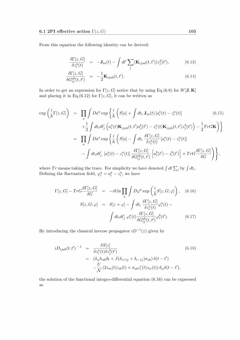
6.1 2PI effective action Γ(z, G) 105
From this equation the following identity can be derived:
δΓ[z, G]δza
i (t)= −Jia(t)−
∫dt′
∑
j
(Kijad(t, t′))zdj (t′), (6.13)
δΓ[z,G]δGab
ij (t, t′)= −1
2Kijab(t, t′). (6.14)
In order to get an expression for Γ[z, G] notice that by using Eq.(6.8) for W [J,K]and placing it in Eq.(6.12) for Γ[z, G], it can be written as
exp(
i
~Γ[z, G]
)=
∏a
∫Daa exp
i
~
(S[a] +
∫dti Jia(t) [aa
i (t)− zai (t)] (6.15)
+12
∫dtidt′j
(aa
i (t)Kijab(t, t′)ab
j(t′)− za
i (t)Kijab(t, t′)zb
j(t′))− 1
2TrGK
)
=∏a
∫Daa exp
i
~
(S[a]−
∫dti
δΓ[z, G]δza
i (t)[aa
i (t)− zai (t)]
−∫
dtidt′j [aai (t)− za
i (t)]δΓ[z,G]
δGabij (t, t′)
[ab
i(t′)− zb
i (t′)]
+ TrGδΓ[z,G]
δG
),
where Tr means taking the trace. For simplicity we have denoted∫
dt∑
i by∫
dti.Defining the fluctuation field, ϕa
i = aai − za
i , we have
Γ[z, G]− TrGδΓ[z, G]
δG= −i~ ln
∏a
∫Dϕa exp
(i
~S[z, G; ϕ]
), (6.16)
S[z,G;ϕ] = S[z + ϕ]−∫
dtiδΓ[z, G]δza
i (t)ϕa
i (t)−∫
dtidt′j ϕai (t)
δΓ[z, G]δGab
ij (t, t′)ϕb
i(t′). (6.17)
By introducing the classical inverse propagator iD−1(z) given by
iDijab(t, t′) −1 =δS[z]
δzai (t)δzb
j(t′)(6.18)
= (δijhab∂t + J(δi+1j + δi−1j)σab) δ(t− t′)
−U
N (2zia(t)zib(t) + σabzci (t)zic(t)) δijδ(t− t′),
the solution of the functional integro-differential equation (6.16) can be expressedas

106Chapter 6 The two particle irreducible effective action (2PI) and the
closed time path (CTP) formalism
Γ[z, G] = S[z] +i
2Tr lnG−1 +
i
2TrD−1(z)G + Γ2[z,G] + const. (6.19)
The quantity Γ2[z, G] is conveniently described in terms of the diagramsgenerated by the interaction terms in S[z + ϕ] which are of cubic and higherorders in ϕ
Sint[z + ϕ] = − U
4N∫
dti(ϕib(t)ϕbi(t))
2
−U
N∫
dtiϕai (t)zia(t)ϕb
i(t)ϕib(t). (6.20)
It consists of all two-particle irreducible vacuum graphs (the diagrams repre-senting these interactions do not become disconnected by cutting two propagatorlines) in the theory with propagators set equal to G and vertices determined bythe interaction terms in S[z + ϕ] .
Since physical processes correspond to vanishing sources J and K, the dynam-ical equations of motion for the mean field and the propagators are found by usingthe expression (6.19) in equations (6.13) and (6.14) , and setting the right handside equal to zero. This procedure leads to the following equations:
hab~∂tzbi (t) = −J(zi+1a(t) + zi−1a(t)) (6.21)
+U
N (zid(t)zdi (t) + G c
ii c(t, t))zia(t)
+U
N ((Giiad(t, t) + Giida(t, t))zdi (t)
−δΓ2[z, G]δza
i (t),
and
G−1ijab(t, t
′) = Dijab(t, t′)−1 − Σijab(t, t′), (6.22)
Σijab(t, t′) ≡ 2iδΓ2[z, G]δGab
ij (t, t′). (6.23)
Equation (6.22) can be rewritten as a partial differential equation suitable forinitial value problems by convolution with G. This differential equation readsexplicitly
hac~∂tG
cbij (t, t′) = −J(Gab
i+1j(t, t′) + Gab
i−1j(t, t′)) +
U
N (zid(t)zdi (t))Gab
ij (t, t′) + (6.24)
2U
N zai (t)Gcb
ij (t, t′)zic(t) + i
∫dt′′kΣ
aikc(t, t
′′)Gcbkj(t
′′, t′) + iδabδijδ(t− t′).
The evolution of za and Gab is determined by Eqs. (6.22) and (6.24) once Γ2[z,G]is specified.

6.2 Perturbative expansion of Γ2(z, G) and approximation schemes 107
6.2 Perturbative expansion of Γ2(z, G) and approxima-tion schemes
The diagrammatic expansion of Γ2 is illustrated in Fig. 6.1, where two andthree-loop vacuum diagrams are shown. The dots where four lines meet representinteraction vertices. The expression corresponding to each vacuum diagramshould be multiplied by a factor (−i)l(i)s−2 where l is the number of solid linesand s the number of loops the diagram contains.
The action Γ including the full diagrammatic series for Γ2 gives the full dy-namics. It is of course not feasible to obtain an exact expression for Γ2 in a closedform. Various approximations for the full 2PI effective action can be obtainedby truncating the diagrammatic expansion for Γ2. Which approximation is mostappropriate depends on the physical problem under consideration.
6.2.1 The standard approaches
1. Mean-field approximation:
If, in Eq. (6.19), we discard all terms to the right of S[z], we recover theDNLSE. This gives us the usual mean-field description, in which the systemremains a pure condensate.
2. One-loop Approximation:
The next approximation consists of discarding Γ2 altogether. This yieldsthe so-called one-loop approximation. The one-loop approximation has anequation for the fluctuations identical to the BdG equations (See chapter 5),however the equation of motion for the condensate does include the deple-tion and anomalous terms. The presence of this terms is necessary for thetime dependent evolution because they guarantee the conservation of particlenumber and energy. The unequal treatment of the condensate and fluctu-ations present in this approximation introduces limitations and makes thisapproach not very attractive for studying the non equilibrium dynamics.
3. Time-dependent Hartree-Fock-Bogoliubov (HFB) approximation:
A truncation of Γ2 retaining only the first order diagram in U, i.e., keepingonly the double-bubble diagram, Fig. 6.1, yields equations of motion for z andG which correspond to the time dependent Hartree-Fock-Bogoliubov (HFB)approximation. This approximation violates Goldstone’s theorem, but con-serves energy and particle number [132, 15, 133]. It is important to point outthat between all the quadratic approximations discussed in chapter 5 onlythe HFB approximation is suitable for describing non equilibrium dynamicsbecause it is the only one that obeys conservation laws. The HFB equationscan also be obtained by using cumulant expansions up to the second-order[136] in which all cumulants containing three or four field operators areneglected. The HFB approximation neglects multiple scattering. It can be
108Chapter 6 The two particle irreducible effective action (2PI) and the
closed time path (CTP) formalism
interpreted as an expansion in terms of Ut/J, (where t is the time of evo-lution) and is good for the description of short time dynamics or weakinteraction strengths. It will be described in more detail in section 6.4.
6.2.2 Higher order expansions
We make a few remarks on the general properties of higher order expansions andthen specialize to two approximations.
• 2PI and Ladder Diagrams
Since the work of Beliaev [63] and Popov [52] it is well known in the literaturethat including higher order terms in a diagrammatic expansion correspondsto renormalizing the bare interaction potential to the four-point vertex (seefor example Ref. [53, 54]), thus accounting for the repeated scattering of thebosons. In particular, in chapter 5 we explicitly showed how by includingthe anomalous average in the equations the bare potential was upgraded inthe off diagonal elements to the many body scattering matrix. In chapter8 we will also show that by taking into account the two-loop contributionof the 2PI effective action, the bare potential in the diagonal terms is alsoupgraded to the many body scattering matrix up to second-order in the lad-der expansion. The two-loop contribution includes diagrams topologicallyidentical to those found by Beliaev, but with the exact propagator insteadof the one-loop propagator. In the dilute gas limit, where the inter-particledistance is large compared with the s-wave scattering length, the ladder di-agrams give the largest contribution to the four-point vertex. To lowestorder in the diluteness parameter, the T-matrix can be approximated by aconstant proportional to the scattering length (the pseudopotential approx-imation). However this approximation is only valid in the weak interactionlimit and neglects all momentum dependencies which appears in the problemas higher order terms. In that sense the 2PI effective action approach allowsus to go beyond the weakly interacting limit in a systematic way and to treatcollisions more accurately.
• Nonlocal Dissipation and Non-Markovian Dynamics
Higher order terms lead to nonlocal equations and dissipation. The presenceof nonlocal terms in the equations of motion is a consequence of the factthat the 2PI effective action really corresponds to a further approximationof the master effective equation [118]. Though strict dissipation can neverbe observed in an energy conserving closed system, characteristic features ofdissipative systems like exponential damping of correlations can be exhibitedonce interactions are properly taken into account.
Non-Markovian dynamics is a generic feature of the 2PI formalism whichyields integro-differential equations of motion. This makes numerical so-lution difficult, but is a necessary price to pay for a fuller account of thequantum dynamics. Many well acknowledged approaches to the quantum

6.2 Perturbative expansion of Γ2(z, G) and approximation schemes 109
kinetics of such systems adopt either explicitly or implicitly a Markovianapproximation [62]. The Markovian approximation assumes that only thecurrent configuration of the system, but not its history, determines its futureevolution. Markovian approximations are made if one assumes instantaneousinteractions, or in the kinetic theory context that the time scales betweenthe duration of binary collisions τ0 and the inverse collision rate τc are well-separated. In the low kinetic energy, weakly interacting regime the timebetween collisions (or mean free path) is long compared to the reaction time(or scattering length): τc >> τ0. The long separation between collisions andthe presence of intermediate weak fluctuations, allow for a rapid decay ofthe temporal and spatial correlations created between collision partners,which one can use to justify the Markovian approximation. However,non-Markovian dynamics needs to be confronted squarely in systems such as thepatterned loaded lattice, in which the lattice which confines the atoms to thebottom of the wells with enhanced interaction effects, accompanied by thelow dimensionality of the system and far-from-equilibrium initial conditions.That is the rationale for our adoption of the CTP 2PI scheme. Now, for thespecifics:
1. Second-order expansion:
A truncation retaining diagrams of second-order in U consists of the double-bubble, the setting-sun and the basketball (see Fig.6.1). By including thesetting-sun and the basketball in the approximations we are taking into ac-count two particle scattering processes [121, 119]. Second-order terms leadto integro- differential equations which depend on the time history of thesystem.
2. Large-N approximation
The 1/N expansion is a controlled non-perturbative approximation schemewhich can be used to study non-equilibrium quantum field dynamics inthe regime of strong interactions[127, 126]. In the large N approach thefield is modelled by N fields and the quantum field generating functionalis expanded in powers of 1/N . In this sense the method is a controlledexpansion in a small parameter, but unlike perturbation theory in the cou-pling constant, which corresponds to an expansion around the vacuum, thelarge N expansion corresponds to an expansion of the theory about a strongquasiclassical field.
6.2.3 Zero mode fluctuactions
In chapter 5 we neglected zero mode fluctuations due to the non perturbativecharacter of the zero mode. In the linearized theory, this approach introduces anartificial infrared divergence in low dimensional models thus the theory is actuallyimproved if the contribution from this mode is neglected all together [96]. However,from a physical point of view the zero mode exists and is quantum in nature. There

110Chapter 6 The two particle irreducible effective action (2PI) and the
closed time path (CTP) formalism
are both fundamental and practical reasons why isolating and subtracting the zeromode is not as compelling in the dynamical evolution we want to describe in thischapter. Firstly, because the 2PI formalism goes beyond the linearized approxi-mation, the zero mode does not have the impact it has in the linearized formalismand it is not clear that subtracting it necessarily leads to a better approximation.Secondly, the initial state that we are going to assume for our analysis is a coherentstate rather than a proper state of the total particle number as will be describedin chapter 7. Moreover, as the total particle number is not very high, quantumfluctuations in the total particle number are real, and non-negligible. Discardingthese fluctuations would spoil the integrity of the formalism. Therefore, in thischapter we shall not attempt to isolate the contributions from the zero mode. Afull non-perturbative treatment in the future is certainly desirable.
6.3 CTP formalism
In order to describe the nonequilibrium dynamics we will now specify the contourof integration in Eqs. (6.22) and (6.24) to be the Schwinger-Keldysh contour [56]along the real-time axis or closed time path (CTP) contour. The Schwinger-Keldysh formalism is a powerful method for deriving real and causal evolutionequations for the expectation values of quantum operators for nonequilibriumfields. The basic idea of the CTP formalism relies on the fact that a diagonalmatrix element of a system at a given time, t = 0, can be expressed as a productof transition matrix elements from t = 0 to t′ and the time-reverse (complexconjugate) matrix element from t′ to 0 by inserting a complete set of states into thismatrix element at the later time t′. Since each term in the product is a transitionmatrix element of the usual or time reversed kind, the standard path integralrepresentation for each one can be introduced. However, to get the generatingfunctional we seek, we have to require that the forward time evolution takes placein the presence of a source J+ but the reversed time evolution takes place in thepresence of a different source J−, otherwise all the dependence on the source dropsout.
The doubling of sources, the fields and integration contours suggest introduc-ing a 2 x 2 matrix notation. This notation has been discussed extensively in theliterature [117, 119]. However we are going to follow Refs. [126] and [127] andintroduce the CTP formalism in our equation of motion by using the compositionrule for transition amplitudes along the time contour in the complex plane. Thisway is cleaner notationally and has the advantage that all the functional formal-ism of the previous section may be taken with the only difference of path orderingaccording to the complex time contour Cctp in the time integrations.
The two-point functions are decomposed as
Gabij (t, t′) = θctp(t, t′)Gab>
ij (t, t′) + θctp(t′, t)Gab<ij (t, t′), (6.25)
where
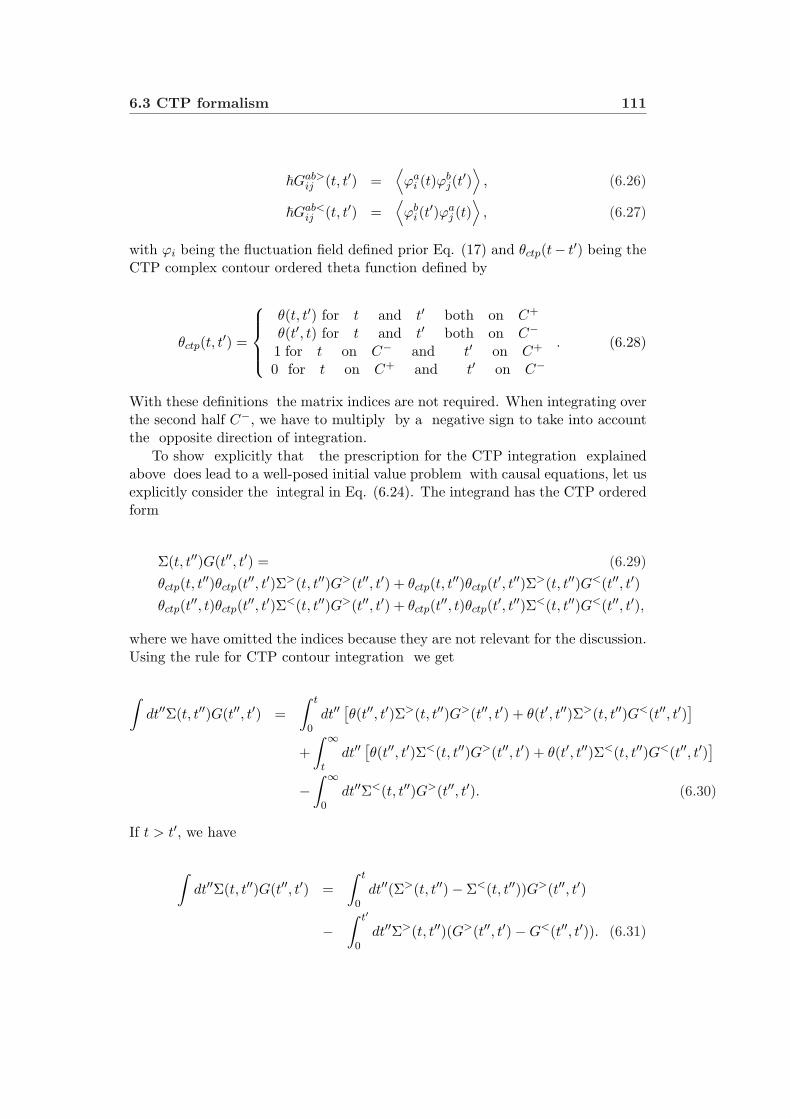
6.3 CTP formalism 111
~Gab>ij (t, t′) =
⟨ϕa
i (t)ϕbj(t
′)⟩
, (6.26)
~Gab<ij (t, t′) =
⟨ϕb
i(t′)ϕa
j (t)⟩
, (6.27)
with ϕi being the fluctuation field defined prior Eq. (17) and θctp(t− t′) being theCTP complex contour ordered theta function defined by
θctp(t, t′) =
θ(t, t′) for t and t′ both on C+
θ(t′, t) for t and t′ both on C−
1 for t on C− and t′ on C+
0 for t on C+ and t′ on C−. (6.28)
With these definitions the matrix indices are not required. When integrating overthe second half C−, we have to multiply by a negative sign to take into accountthe opposite direction of integration.
To show explicitly that the prescription for the CTP integration explainedabove does lead to a well-posed initial value problem with causal equations, let usexplicitly consider the integral in Eq. (6.24). The integrand has the CTP orderedform
Σ(t, t′′)G(t′′, t′) = (6.29)θctp(t, t′′)θctp(t′′, t′)Σ>(t, t′′)G>(t′′, t′) + θctp(t, t′′)θctp(t′, t′′)Σ>(t, t′′)G<(t′′, t′)θctp(t′′, t)θctp(t′′, t′)Σ<(t, t′′)G>(t′′, t′) + θctp(t′′, t)θctp(t′, t′′)Σ<(t, t′′)G<(t′′, t′),
where we have omitted the indices because they are not relevant for the discussion.Using the rule for CTP contour integration we get
∫dt′′Σ(t, t′′)G(t′′, t′) =
∫ t
0dt′′
[θ(t′′, t′)Σ>(t, t′′)G>(t′′, t′) + θ(t′, t′′)Σ>(t, t′′)G<(t′′, t′)
]
+∫ ∞
tdt′′
[θ(t′′, t′)Σ<(t, t′′)G>(t′′, t′) + θ(t′, t′′)Σ<(t, t′′)G<(t′′, t′)
]
−∫ ∞
0dt′′Σ<(t, t′′)G>(t′′, t′). (6.30)
If t > t′, we have
∫dt′′Σ(t, t′′)G(t′′, t′) =
∫ t
0dt′′(Σ>(t, t′′)− Σ<(t, t′′))G>(t′′, t′)
−∫ t′
0dt′′Σ>(t, t′′)(G>(t′′, t′)−G<(t′′, t′)). (6.31)

112Chapter 6 The two particle irreducible effective action (2PI) and the
closed time path (CTP) formalism
On the other hand, if t < t′
∫dt′′Σ(t, t′′)G(t′′, t′) =
∫ t
0dt′′(Σ>(t, t′′)− Σ<(t, t′′))G<(t′′, t′)
−∫ t′
0dt′′Σ<(t, t′′)(G>(t′′, t′)−G<(t′′, t′)). (6.32)
The above equations are explicitly causal.It is convenient to express the evolution equations in terms of two independenttwo-point functions which can be associated to the expectation values of thecommutator and the anti-commutator of the fields. We define, following Ref. [127]the functions
G(F )abij (t, t′) =
12
(Gab>
ij (t, t′) + Gab<ij (t, t′)
)(6.33)
G(ρ)abij (t, t′) = i
(Gab>
ij (t, t′)−Gab<ij (t, t′)
), (6.34)
where the (F ) functions are usually called statistical propagators and the (ρ) arecalled spectral functions [137]. With these definitions Eq.(6.24) can be rewrittenas:
hac~∂tG
(F )cbij (t, t′) = −J
(G
(F )abi+1j (t, t′) + G
(F )abi−1j (t, t′)
)+
U
N(zic(t)zc
i (t))G(F )abij (t, t′)
)+
2U
N(zai (t)G(F )cb
ij (t, t′)zic(t))
+∫ t
0dt′′kΣ
(ρ)acik (t, t′′)G(F ) b
kj c (t′′, t′)
−∫ t′
0dt′′kΣ
(F )acik (t, t′′)G(ρ)b
kjc (t′′, t′), (6.35)
hac~∂tG
(ρ)cbij (t, t′) = −J
(G
(ρ)abi+1j (t, t′) + G
(ρ)abi−1j (t, t′)
)+
U
N(zic(t)zc
i (t))G(ρ)abij (t, t′
)+
2U
N(zai (t)G(ρ)cb
ij (t, t′)zic(t))
+∫ t
t′dt′′kΣ
(ρ)acik (t, t′′)G(ρ)b
kjc (t′′, t′).(6.36)
In particular, we define the normal, ρ, and anomalous, m, spectral and statisticalfunctions as
G21(F )ij (t, t′) ≡ ρ
(F )ij (t, t′) =
12
⟨ϕ†i (t)ϕj(t′) + ϕj(t′)ϕ
†i (t)
⟩, (6.37)
G21(ρ)ij (t, t′) ≡ ρ
(ρ)ij (t, t′) = i
⟨ϕ†i (t)ϕj(t′)− ϕj(t′)ϕ
†i (t)
⟩, (6.38)
G11(F )ij (t, t′) ≡ m
(F )ij (t, t′) =
12
⟨ϕi(t)ϕj(t′) + ϕj(t′)ϕi(t)
⟩, (6.39)
G11(ρ)ij (t, t′) ≡ m
(ρ)ij (t, t′) = i
⟨ϕi(t)ϕj(t′)− ϕj(t′)ϕi(t)
⟩. (6.40)

6.4 HFB approximation 113
With these relations in place, we now proceed to derive the time evolutionequations for the mean field and the two-point functions from the 2PI-CTP effec-tive action for the Bose-Hubbard model under the three approximations describedbefore.
6.4 HFB approximation
6.4.1 Equations of motion
The HFB equations include the leading order contribution of Γ2. They describethe coupled dynamics of condensate and non-condensate atoms which arise fromthe most important scattering processes which are direct, exchange and pair ex-citations. The basic damping mechanisms present in the HFB approximation areLandau and Beliaev damping associated with the decay of an elementary exci-tation into a pair of excitations in the presence of condensate atoms[133, 134].However, these kinds of damping 1 found in the HFB approximation (due to phasemixing, as in the Vlasov equation citeBalescu) are different in nature from thecollisional dissipation (as in the Boltzmann equation) responsible for thermaliza-tion processes. Multiple scattering processes are neglected in this approximation.We expect the HFB equations to give a good description of the dynamics in thecollisionless regime when interparticle collisions play a minor role.
The leading order contribution of Γ2 is represented by the double-bubblediagram. Its contribution to Γ2 is z independent and has an analytic expressionof the form
Γ(1)2 [G] = (6.41)
− U
4N∫
dti
(G a
iia(t, t)Gbiib(t, t) + 2Giiab(t, t)Gab
ii (t, t))
,
the factor of two arises because the direct and exchange terms are identical.Using the first order expression for Γ2 in Eqs. (6.22) and (6.24) yields the
following equations of motion.
hab~∂tz
bi (t) = ζz
HFB, (6.42)
ζzHFB ≡ −J
(zai+1(t) + za
i−1(t))
+U
N(zid(t)zd
i (t) + G dii d(t, t)
)zai (t)
+2U
N(zib(t)Gab
ii (t, t))
, (6.43)
1we make a distinction between the meaning of the words ‘damping’ and ‘dissipation’, theformer referring simply to the phenomenological decay of some function, the latter with theoreticalmeaning, e.g., in the Boltzmann sense.
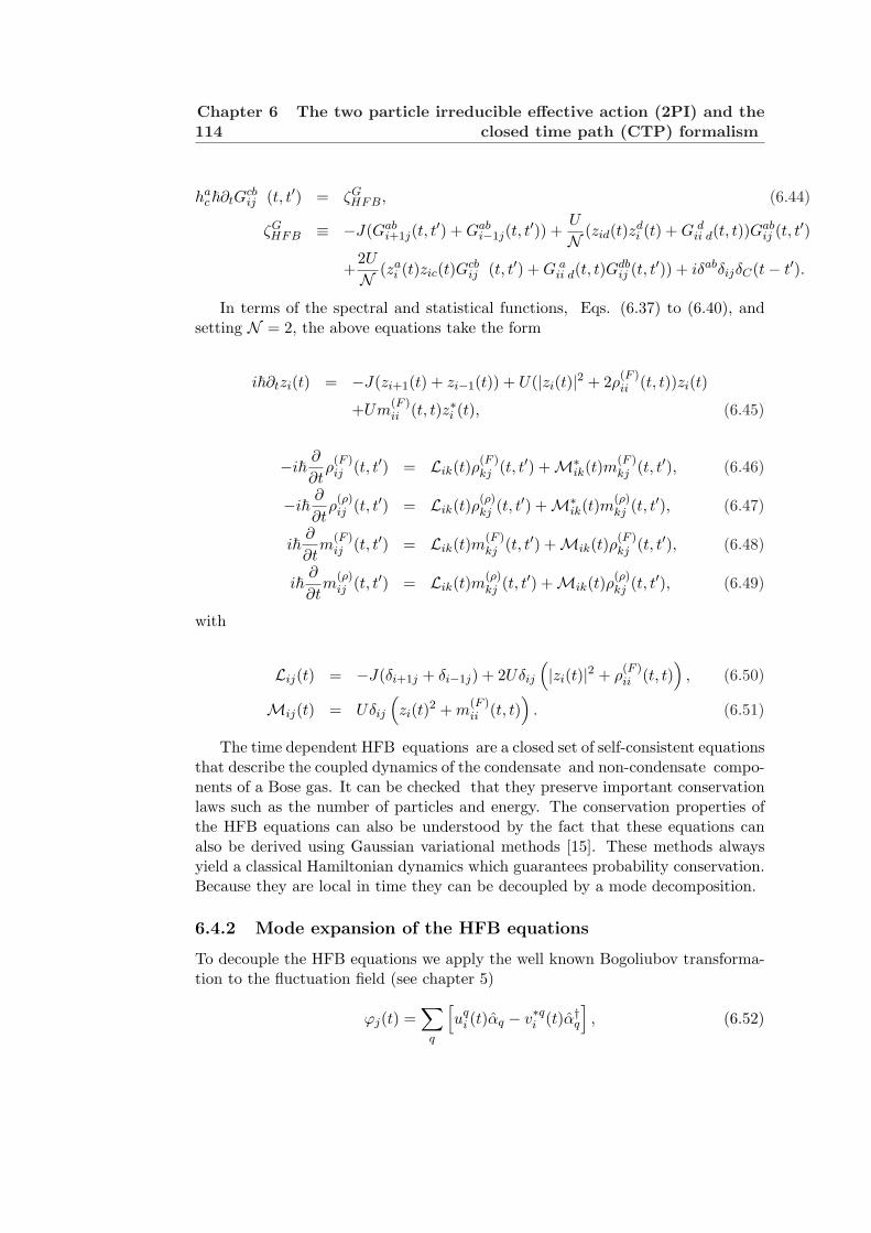
114Chapter 6 The two particle irreducible effective action (2PI) and the
closed time path (CTP) formalism
hac~∂tG
cbij (t, t′) = ζG
HFB, (6.44)
ζGHFB ≡ −J(Gab
i+1j(t, t′) + Gab
i−1j(t, t′)) +
U
N (zid(t)zdi (t) + G d
ii d(t, t))Gabij (t, t′)
+2U
N (zai (t)zic(t)Gcb
ij (t, t′) + G aii d(t, t)G
dbij (t, t′)) + iδabδijδC(t− t′).
In terms of the spectral and statistical functions, Eqs. (6.37) to (6.40), andsetting N = 2, the above equations take the form
i~∂tzi(t) = −J(zi+1(t) + zi−1(t)) + U(|zi(t)|2 + 2ρ(F )ii (t, t))zi(t)
+Um(F )ii (t, t)z∗i (t), (6.45)
−i~∂
∂tρ(F )ij (t, t′) = Lik(t)ρ
(F )kj (t, t′) +M∗
ik(t)m(F )kj (t, t′), (6.46)
−i~∂
∂tρ(ρ)ij (t, t′) = Lik(t)ρ
(ρ)kj (t, t′) +M∗
ik(t)m(ρ)kj (t, t′), (6.47)
i~∂
∂tm
(F )ij (t, t′) = Lik(t)m
(F )kj (t, t′) +Mik(t)ρ
(F )kj (t, t′), (6.48)
i~∂
∂tm
(ρ)ij (t, t′) = Lik(t)m
(ρ)kj (t, t′) +Mik(t)ρ
(ρ)kj (t, t′), (6.49)
with
Lij(t) = −J(δi+1j + δi−1j) + 2Uδij
(|zi(t)|2 + ρ
(F )ii (t, t)
), (6.50)
Mij(t) = Uδij
(zi(t)2 + m
(F )ii (t, t)
). (6.51)
The time dependent HFB equations are a closed set of self-consistent equationsthat describe the coupled dynamics of the condensate and non-condensate compo-nents of a Bose gas. It can be checked that they preserve important conservationlaws such as the number of particles and energy. The conservation properties ofthe HFB equations can also be understood by the fact that these equations canalso be derived using Gaussian variational methods [15]. These methods alwaysyield a classical Hamiltonian dynamics which guarantees probability conservation.Because they are local in time they can be decoupled by a mode decomposition.
6.4.2 Mode expansion of the HFB equations
To decouple the HFB equations we apply the well known Bogoliubov transforma-tion to the fluctuation field (see chapter 5)
ϕj(t) =∑
q
[uq
i (t)αq − v∗qi (t)α†q], (6.52)
6.4 HFB approximation 115
where (αq, α†q) are time independent creation and annihilation quasiparticle oper-
ators and all the time dependence is absorbed in the amplitudes uqi (t), v
∗qi (t).
To ensure that the quasiparticle transformation is canonical, the amplitudes mustfulfill the relations
∑
i
[uq
i (t)u∗ki (t)− vq
i (t)v∗ki (t)
]= δqk, (6.53)
∑
i
[uq
i (t)vki (t)− vq
i (t)uki (t)
]= 0. (6.54)
In the zero temperature limit, where the quasiparticle occupation number vanishes,⟨α†qαk
⟩= 0, the statistical and spectral functions take the form
ρ(F )ij (t, t′) =
12
∑q
(vqi (t)v
∗qj (t′) + uq
j(t′)u∗qi (t)
), (6.55)
ρ(ρ)ij (t, t′) = i
∑q
(vqi (t)v
∗qj (t′)− uq
j(t′)u∗qi (t)
), (6.56)
m(F )ij (t, t′) = −1
2
∑q
(uq
i (t)v∗qj (t′) + uq
j(t′)v∗qi (t)
), (6.57)
m(ρ)ij (t, t′) = −i
∑q
(uq
i (t)v∗qj (t′)− uq
j(t′)v∗qi (t)
). (6.58)
Notice that at equal time and position due to Eqs.(6.53) and (6.54), ρ(F )ii (t, t)
and m(F )ii (t, t) satisfy
ρ(F )ii (t, t) =
∑q
|vqi (t)|2 +
12
(6.59)
m(F )ii (t, t) = −
∑q
uqi (t)v
∗qi (t). (6.60)
Replacing Eqs. (6.59)-(6.60) into Eqs. (6.45)-(6.49) and using the constraints(6.53) -(6.54) we recover the standard time dependent equations for the quasipar-ticle amplitudes
i~∂
∂zi(t) (6.61)
= −J(zi+1(t) + zi−1(t)) + U(|zi(t)|2 + 2ρ(F )ii (t, t))zi(t) + Um
(F )ii (t, t)z∗i (t),
116Chapter 6 The two particle irreducible effective action (2PI) and the
closed time path (CTP) formalism
i~∂
∂tuq
i (t) (6.62)
= −J(uqi+1(t) + uq
i−1(t)) + 2U(|zi(t)|2 + ρ(F )ii (t, t))uq
i (t)− U(m(F )ii (t, t) + zi(t)
2)vqi (t),
−i~∂
∂tvqi (t) = (6.63)
−J(vqi+1(t) + vq
i−1(t))) + 2U(|zi(t)|2 + ρ(F )ii (t, t))vq
i (t)− U(m∗(F )ii (t, t) + zi(t)∗2)u
qi (t).
If we compare Eqs. (6.61)-(6.63) with their time independent version, Eqs. (5.27)to (5.87), we notice that the equations are identical as they should be if we replacei~ ∂
∂tuqi → ωHFBuq
i , i~ ∂∂tv
qi → ωHFBvq
i and i~∂tzi → µHFBzi. The factor of 1/2difference between ρ
(F )ii and ρii (see Eq. (5.19)) just leads to a trivial renormaliza-
tion of the chemical potential. In the time dependent equations we have includedthe zero mode fluctuations, which were neglected in Eqs. (5.27) to (5.87). Hencewe do not need the cHFB±
s variables, which simply keep the orthogonality betweenof the condensate and the excitations. Eqs. (6.61) -(6.63) correspond to a set ofM(2M + 1) coupled ordinary differential equations, where M is the total numberof lattice sites. They can be solved using standard time propagation algorithms.Once the time dependent quasiparticle amplitudes are calculated we can derive thedynamics of physical observables constructed from them as a function of time,such as the average number of particles in a well ni(t), etc.
6.5 Second-order expansion
6.5.1 Equations of motion
Full second-order
The second-order contribution to Γ2 is described in terms of the setting-sun Fig. 6.1band the basketball Fig. 6.1c diagrams. The basketball diagram is independent ofthe mean-field and is constructed with only quartic vertices. The setting-sundiagram depends on z and contains only three-point vertices. The second-orderΓ(2)
2 effective action can be written as
Γ(2)2 [z, G] = (6.64)
i
(U
N)2 ∫
dtidtjzib(t)zjb′(t′)×(Gbb′
ij (t, t′)Gijdd′(t, t′)Gdd′ij (t, t′) + 2Gbd′
ij (t, t′)Gijdd′(t, t′)Gdb′ij (t, t′)
)+
i
(U
2N)2 ∫
dtidt′j(Gijbb′(t, t′)Gbb′
ij (t, t′)Gijdd′(t, t′)Gdd′
ij (t, t′)+
2Gijbb′(t, t′)Gbd′
ij (t, t′)Gijdd′(t, t′)Gdb′
ij (t, t′))
.
6.5 Second-order expansion 117
To simplify the notation, let us introduce the following definitions [127]:
Πij(t, t′) = −12Gijab(t, t′)Gab
ij (t, t′), (6.65)
Ξijab(t, t′) = −D(t, t′)Gijab(t, t
′), (6.66)
D(t, t′) = zib(t)zja(t′)Gbaij (t, t′)−Πij(t, t
′), (6.67)
Λ bij a(t, t
′) = −Gcbij (t, t
′)Gijca(t, t′), (6.68)
Λ bij a(t, t
′) = −G bcij (t, t′)Gijac(t, t
′), (6.69)
Θacij (t, t′) = −(zid(t)zjb(t′) + Gijdb(t, t′))Gab
ij (t, t′)Gdcij (t, t′) + Ξac
ij (t, t′).(6.70)
With the above definitions we find from Eqs. (6.22) and (6.24) the followingequations of motion:
hab~∂tz
bi (t) = ζz
HFB + (6.71)
i
(2U
N)2 ∫
dt′j zjb(t′)(Πij(t, t′)Gba
ji (t′, t) + Λ bij c(t, t
′)Gacij (t, t′)
),
hac~∂tG
cbij (t, t′) = ζG
HFB + (6.72)
i
(2U
N)2
zai (t)
∫dt′′kzkc(t′′)
(Πik(t, t′′)Gcb
kj(t′′, t′) + Λ c
ik d(t, t′′)Gdb
kj(t′′, t′)
)
+i
(2U
N)2 ∫
dt′′(Θ a
ik d(t, t′′) + Λca
ik (t, t′′)zic(t)zkd(t′′))Gdb
kj (t′′, t′),
where ζzHFB and ζG
HFB are defined in Eqs. (6.43) and (6.45).
To get explicit expressions of the equations of motion in terms of ρ(F,ρ) andm(F,ρ) we introduce the functions
Ω(F )ij [f ,g] = f (F )
ij (ti, tj)g(F )ij (ti, tj)− 1
4
(f (ρ)ij (ti, tj)g
(ρ)ij (ti, tj)
), (6.73)
Ω(ρ)ij [f ,g] = f (F )
ij (ti, tj)g(ρ)ij (ti, tj) + f (ρ)
ij (t, t′)g(F )ij (ti, tj). (6.74)
Using the spectral and statistical functions and setting the number of fieldsN equalto 2, the equations of motion derived under the full second-order approximationcan be written as:
118Chapter 6 The two particle irreducible effective action (2PI) and the
closed time path (CTP) formalism
i~∂tizi = −J(zi+1(ti) + zi−1(ti)) + U(|zi|2 + 2ρ(F )ii )zi + Um
(F )ii z∗i (6.75)
−2U2∑
k
∫ ti
0dtk
(zkΩ
(ρ)ik [ρ, ρ∗] + zkΩ
(ρ)ik [m,m∗] + z∗kΩ(ρ)
ik [m, ρ])
ρ(F )ki
−2U2∑
k
∫ ti
0
(z∗kΩ(ρ)
ik [ρ, ρ∗] + z∗kΩ(ρ)ik [m,m∗] + zkΩ
(ρ)ik [m∗, ρ∗]
)m
(F )ki
+2U2∑
k
∫ ti
0dtk
(zkΩ
(F )ik [ρ, ρ∗] + zkΩ
(F )ik [m, m∗] + z∗kΩ(F )
ik [m, ρ])
ρ(ρ)ki
+2U2∑
k
∫ ti
0
(z∗kΩ(F )
ik [ρ, ρ∗] + z∗kΩ(F )ik [m,m∗] + zkΩ
(F )ik [m∗, ρ∗]
)m
(ρ)ki ,
−i~∂tiρ(F )ij = (6.76)
−J(ρ(F )i+1j(ti, tj) + ρ
(F )i−1j(ti, tj)) + 2U(|zi|2 + ρ
(F )ii )ρ(F )
ij + U(m∗(F )ii + z∗2i )m(F )
ij
−2U2∑
k
∫ ti
0dtk
(ziz
∗kΩ(ρ)
ik [ρ, ρ] + 2zizkΩ(ρ)ik [ρ, m∗] + 2z∗i z∗kΩ(ρ)
ik [m, ρ])
ρ(F )kj
−2U2∑
k
∫ ti
0dtk
(Ω(ρ)
ik [ρ, ∆] + 2z∗i zk
(Ω(ρ)
ik [ρ, ρ∗] + Ω(ρ)ik [m,m∗]
))ρ(F )kj
−2U2∑
k
∫ ti
0dtk
(2ziz
∗kΩ(ρ)
ik [m∗, ρ] + zizkΩ(ρ)ik [m∗,m∗] + 2z∗i zkΩ
(ρ)ik [ρ∗,m∗]
)m
(F )kj
−2U2∑
k
∫ ti
0dtk
(Ω(ρ)
ik [m∗,Υ] + z∗i z∗k(2Ω(ρ)
ik [ρ, ρ∗] + 2Ω(ρ)ik [m, m∗]
))m
(F )kj
+2U2∑
k
∫ tj
0dtk
(ziz
∗kΩ(F )
ik [ρ, ρ] + 2zizkΩ(F )ik [ρ,m∗] + 2z∗i z∗kΩ(F )
ik [m, ρ])
ρ(ρ)kj
+2U2∑
k
∫ tj
0dtk
(Ω(F )
ik [ρ,∆] + 2z∗i zk
(Ω(F )
ik [ρ, ρ∗] + Ω(F )ik [m,m∗]
))ρ(ρ)kj
+2U2∑
k
∫ tj
0dtk
(2ziz
∗kΩ(F )
ik [m∗, ρ] + zizkΩ(F )ik [m∗,m∗] + 2z∗i zkΩ
(F )ik [ρ∗, m∗]
)m
(ρ)kj
+2U2∑
k
∫ tj
0dtk
(Ω(F )
ik [m∗,Υ] + 2z∗i z∗k(Ω(F )
ik [ρ, ρ∗] + Ω(F )ik [m,m∗]
))m
(F )kj ,
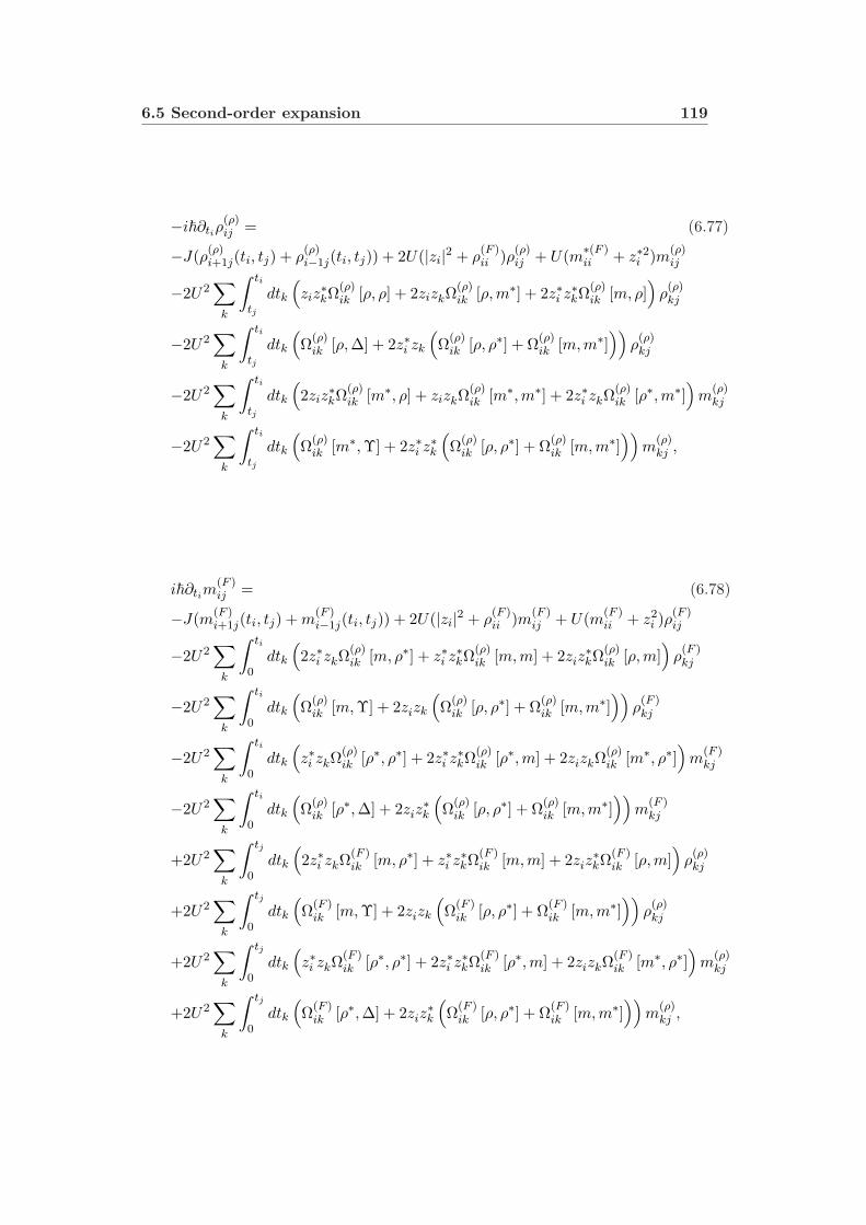
6.5 Second-order expansion 119
−i~∂tiρ(ρ)ij = (6.77)
−J(ρ(ρ)i+1j(ti, tj) + ρ
(ρ)i−1j(ti, tj)) + 2U(|zi|2 + ρ
(F )ii )ρ(ρ)
ij + U(m∗(F )ii + z∗2i )m(ρ)
ij
−2U2∑
k
∫ ti
tj
dtk
(ziz
∗kΩ(ρ)
ik [ρ, ρ] + 2zizkΩ(ρ)ik [ρ, m∗] + 2z∗i z∗kΩ(ρ)
ik [m, ρ])
ρ(ρ)kj
−2U2∑
k
∫ ti
tj
dtk
(Ω(ρ)
ik [ρ, ∆] + 2z∗i zk
(Ω(ρ)
ik [ρ, ρ∗] + Ω(ρ)ik [m,m∗]
))ρ(ρ)kj
−2U2∑
k
∫ ti
tj
dtk
(2ziz
∗kΩ(ρ)
ik [m∗, ρ] + zizkΩ(ρ)ik [m∗,m∗] + 2z∗i zkΩ
(ρ)ik [ρ∗,m∗]
)m
(ρ)kj
−2U2∑
k
∫ ti
tj
dtk
(Ω(ρ)
ik [m∗,Υ] + 2z∗i z∗k(Ω(ρ)
ik [ρ, ρ∗] + Ω(ρ)ik [m,m∗]
))m
(ρ)kj ,
i~∂tim(F )ij = (6.78)
−J(m(F )i+1j(ti, tj) + m
(F )i−1j(ti, tj)) + 2U(|zi|2 + ρ
(F )ii )m(F )
ij + U(m(F )ii + z2
i )ρ(F )ij
−2U2∑
k
∫ ti
0dtk
(2z∗i zkΩ
(ρ)ik [m, ρ∗] + z∗i z∗kΩ(ρ)
ik [m,m] + 2ziz∗kΩ(ρ)
ik [ρ,m])
ρ(F )kj
−2U2∑
k
∫ ti
0dtk
(Ω(ρ)
ik [m,Υ] + 2zizk
(Ω(ρ)
ik [ρ, ρ∗] + Ω(ρ)ik [m,m∗]
))ρ(F )kj
−2U2∑
k
∫ ti
0dtk
(z∗i zkΩ
(ρ)ik [ρ∗, ρ∗] + 2z∗i z∗kΩ(ρ)
ik [ρ∗,m] + 2zizkΩ(ρ)ik [m∗, ρ∗]
)m
(F )kj
−2U2∑
k
∫ ti
0dtk
(Ω(ρ)
ik [ρ∗, ∆] + 2ziz∗k
(Ω(ρ)
ik [ρ, ρ∗] + Ω(ρ)ik [m,m∗]
))m
(F )kj
+2U2∑
k
∫ tj
0dtk
(2z∗i zkΩ
(F )ik [m, ρ∗] + z∗i z∗kΩ(F )
ik [m,m] + 2ziz∗kΩ(F )
ik [ρ,m])
ρ(ρ)kj
+2U2∑
k
∫ tj
0dtk
(Ω(F )
ik [m,Υ] + 2zizk
(Ω(F )
ik [ρ, ρ∗] + Ω(F )ik [m,m∗]
))ρ(ρ)kj
+2U2∑
k
∫ tj
0dtk
(z∗i zkΩ
(F )ik [ρ∗, ρ∗] + 2z∗i z∗kΩ(F )
ik [ρ∗, m] + 2zizkΩ(F )ik [m∗, ρ∗]
)m
(ρ)kj
+2U2∑
k
∫ tj
0dtk
(Ω(F )
ik [ρ∗, ∆] + 2ziz∗k
(Ω(F )
ik [ρ, ρ∗] + Ω(F )ik [m,m∗]
))m
(ρ)kj ,

120Chapter 6 The two particle irreducible effective action (2PI) and the
closed time path (CTP) formalism
i~∂tim(ρ)ij = (6.79)
−J(m(ρ)i+1j(ti, tj) + m
(ρ)i−1j(ti, tj)) + 2U(|zi|2 + ρ
(F )ii )m(ρ)
ij + U(m(F )ii + z2
i )ρ(ρ)ij
+2U2∑
k
∫ ti
tj
dtk
(2z∗i zkΩ
(ρ)ik [m, ρ∗] + z∗i z∗kΩ(ρ)
ik [m,m] + 2ziz∗kΩ(ρ)
ik [ρ,m])
ρ(ρ)kj
+2U2∑
k
∫ ti
tj
dtk
(Ω(ρ)
ik [m,Υ] + zizk
(2Ω(ρ)
ik [ρ, ρ∗] + 2Ω(ρ)ik [m,m∗]
))ρ(ρ)kj
+2U2∑
k
∫ ti
tj
dtk
(z∗i zkΩ
(ρ)ik [ρ∗, ρ∗] + 2z∗i z∗kΩ(ρ)
ik [ρ∗,m] + 2zizkΩ(ρ)ik [m∗, ρ∗]
)m
(ρ)kj
+2U2∑
k
∫ ti
tj
dtk
(Ω(ρ)
ik [ρ∗, ∆] + 2ziz∗k
(Ω(ρ)
ik [ρ, ρ∗] + Ω(ρ)ik [m,m∗]
))m
(ρ)kj ,
with
∆(F,ρ)ij = Ω(F,ρ)
ij [ρ, ρ∗] + 2Ω(F,ρ)ij [m, m∗] , (6.80)
Υ(F,ρ)ij = 2Ω(F,ρ)
ij [ρ, ρ∗] + Ω(F,ρ)ij [m, m∗] . (6.81)
In the above equations we adopted the notation zk meaning zk(tk) for thecondensate and mkj and ρkj meaning mkj(tk, tj) and ρkj(tk, tj) respectively forthe two point functions. These notation is also going to be used in the equationsfor the 1/N expansion.
2PI-1/N expansion
The 2PI effective action is a singlet under O(N ) rotations. It can be shown thatall graphs contained in an O(N ) expansion can be built from the irreducibleinvariants[127]: z2, T r(Gn) and Tr(zzGn) , with n < N . The factors of N ina single graph contributing to the same 1/N expansion then have two origins: afactor of N from each irreducible invariant and a factor of 1/N from each vertex.The leading order large N approximation scales proportional to N , the next toleading order (NLO) contributions are of order 1 and so on. At leading order onlythe first term of Eq. (6.42) contributes. At the next to leading order level, if wetruncate up to second-order in the coupling strength, the double-bubble is totallyincluded but only certain parts of the setting-sun and basketball diagrams are: thefirst term in both of the integrals of Eq. (6.64),
Γ(2)1/N2 [z,G] = i
(U
N)2 ∫
dtidtjzib(t)zjb′(t′)(Gbb′
ij (t, t′)Gijdd′(t, t′)Gdd′ij (t, t′)
)+
i
(U
2N)2 ∫
dtidt′j(Gijbb′(t, t′)Gbb′
ij (t, t′)Gijdd′(t, t′)Gdd′
ij (t, t′))
. (6.82)
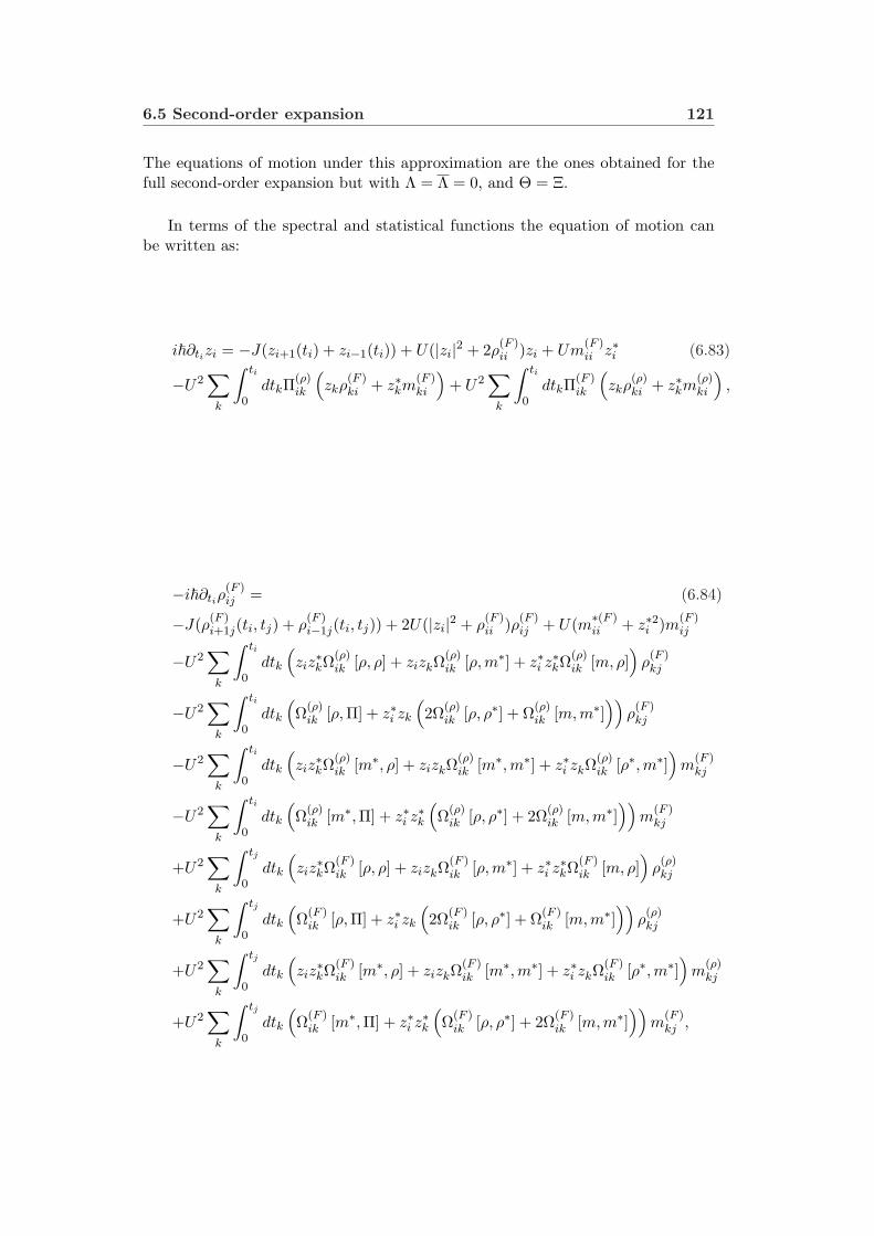
6.5 Second-order expansion 121
The equations of motion under this approximation are the ones obtained for thefull second-order expansion but with Λ = Λ = 0, and Θ = Ξ.
In terms of the spectral and statistical functions the equation of motion canbe written as:
i~∂tizi = −J(zi+1(ti) + zi−1(ti)) + U(|zi|2 + 2ρ(F )ii )zi + Um
(F )ii z∗i (6.83)
−U2∑
k
∫ ti
0dtkΠ
(ρ)ik
(zkρ
(F )ki + z∗km
(F )ki
)+ U2
∑
k
∫ ti
0dtkΠ
(F )ik
(zkρ
(ρ)ki + z∗km
(ρ)ki
),
−i~∂tiρ(F )ij = (6.84)
−J(ρ(F )i+1j(ti, tj) + ρ
(F )i−1j(ti, tj)) + 2U(|zi|2 + ρ
(F )ii )ρ(F )
ij + U(m∗(F )ii + z∗2i )m(F )
ij
−U2∑
k
∫ ti
0dtk
(ziz
∗kΩ(ρ)
ik [ρ, ρ] + zizkΩ(ρ)ik [ρ,m∗] + z∗i z∗kΩ(ρ)
ik [m, ρ])
ρ(F )kj
−U2∑
k
∫ ti
0dtk
(Ω(ρ)
ik [ρ,Π] + z∗i zk
(2Ω(ρ)
ik [ρ, ρ∗] + Ω(ρ)ik [m,m∗]
))ρ(F )kj
−U2∑
k
∫ ti
0dtk
(ziz
∗kΩ(ρ)
ik [m∗, ρ] + zizkΩ(ρ)ik [m∗,m∗] + z∗i zkΩ
(ρ)ik [ρ∗,m∗]
)m
(F )kj
−U2∑
k
∫ ti
0dtk
(Ω(ρ)
ik [m∗, Π] + z∗i z∗k(Ω(ρ)
ik [ρ, ρ∗] + 2Ω(ρ)ik [m,m∗]
))m
(F )kj
+U2∑
k
∫ tj
0dtk
(ziz
∗kΩ(F )
ik [ρ, ρ] + zizkΩ(F )ik [ρ,m∗] + z∗i z∗kΩ(F )
ik [m, ρ])
ρ(ρ)kj
+U2∑
k
∫ tj
0dtk
(Ω(F )
ik [ρ,Π] + z∗i zk
(2Ω(F )
ik [ρ, ρ∗] + Ω(F )ik [m,m∗]
))ρ(ρ)kj
+U2∑
k
∫ tj
0dtk
(ziz
∗kΩ(F )
ik [m∗, ρ] + zizkΩ(F )ik [m∗,m∗] + z∗i zkΩ
(F )ik [ρ∗,m∗]
)m
(ρ)kj
+U2∑
k
∫ tj
0dtk
(Ω(F )
ik [m∗, Π] + z∗i z∗k(Ω(F )
ik [ρ, ρ∗] + 2Ω(F )ik [m,m∗]
))m
(F )kj ,
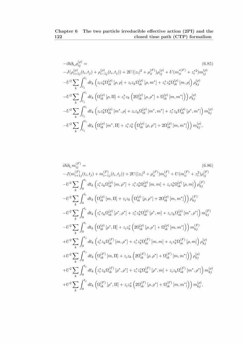
122Chapter 6 The two particle irreducible effective action (2PI) and the
closed time path (CTP) formalism
−i~∂tiρ(ρ)ij = (6.85)
−J(ρ(ρ)i+1j(ti, tj) + ρ
(ρ)i−1j(ti, tj)) + 2U(|zi|2 + ρ
(F )ii )ρ(ρ)
ij + U(m∗(F )ii + z∗2i )m(ρ)
ij
−U2∑
k
∫ ti
tj
dtk
(ziz
∗kΩ(ρ)
ik [ρ, ρ] + zizkΩ(ρ)ik [ρ,m∗] + z∗i z∗kΩ(ρ)
ik [m, ρ])
ρ(ρ)kj
−U2∑
k
∫ ti
tj
dtk
(Ω(ρ)
ik [ρ, Π] + z∗i zk
(2Ω(ρ)
ik [ρ, ρ∗] + Ω(ρ)ik [m,m∗]
))ρ(ρ)kj
−U2∑
k
∫ ti
tj
dtk
(ziz
∗kΩ(ρ)
ik [m∗, ρ] + zizkΩ(ρ)ik [m∗,m∗] + z∗i zkΩ
(ρ)ik [ρ∗, m∗]
)m
(ρ)kj
−U2∑
k
∫ ti
tj
dtk
(Ω(ρ)
ik [m∗,Π] + z∗i z∗k(Ω(ρ)
ik [ρ, ρ∗] + 2Ω(ρ)ik [m,m∗]
))m
(ρ)kj ,
i~∂tim(F )ij = (6.86)
−J(m(F )i+1j(ti, tj) + m
(F )i−1j(ti, tj)) + 2U(|zi|2 + ρ
(F )ii )m(F )
ij + U(m(F )ii + z2
i )ρ(F )ij
−U2∑
k
∫ ti
0dtk
(z∗i zkΩ
(ρ)ik [m, ρ∗] + z∗i z∗kΩ(ρ)
ik [m,m] + ziz∗kΩ(ρ)
ik [ρ,m])
ρ(F )kj
−U2∑
k
∫ ti
0dtk
(Ω(ρ)
ik [m, Π] + zizk
(Ω(ρ)
ik [ρ, ρ∗] + 2Ω(ρ)ik [m,m∗]
))ρ(F )kj
−U2∑
k
∫ ti
0dtk
(z∗i zkΩ
(ρ)ik [ρ∗, ρ∗] + z∗i z∗kΩ(ρ)
ik [ρ∗,m] + zizkΩ(ρ)ik [m∗, ρ∗]
)m
(F )kj
−U2∑
k
∫ ti
0dtk
(Ω(ρ)
ik [ρ∗, Π] + ziz∗k
(2Ω(ρ)
ik [ρ, ρ∗] + Ω(ρ)ik [m,m∗]
))m
(F )kj
+U2∑
k
∫ tj
0dtk
(z∗i zkΩ
(F )ik [m, ρ∗] + z∗i z∗kΩ(F )
ik [m,m] + ziz∗kΩ(F )
ik [ρ,m])
ρ(ρ)kj
+U2∑
k
∫ tj
0dtk
(Ω(F )
ik [m, Π] + zizk
(2Ω(F )
ik [ρ, ρ∗] + Ω(F )ik [m,m∗]
))ρ(ρ)kj
+U2∑
k
∫ tj
0dtk
(z∗i zkΩ
(F )ik [ρ∗, ρ∗] + z∗i z∗kΩ(F )
ik [ρ∗,m] + zizkΩ(F )ik [m∗, ρ∗]
)m
(ρ)kj
+U2∑
k
∫ tj
0dtk
(Ω(F )
ik [ρ∗, Π] + ziz∗k
(2Ω(F )
ik [ρ, ρ∗] + Ω(F )ik [m,m∗]
))m
(ρ)kj ,

6.5 Second-order expansion 123
i~∂tim(ρ)ij = (6.87)
−J(m(ρ)i+1j(ti, tj) + m
(ρ)i−1j(ti, tj)) + 2U(|zi|2 + ρ
(F )ii )m(ρ)
ij + U(m(F )ii + z2
i )ρ(ρ)ij
+U2∑
k
∫ ti
tj
dtk
(z∗i zkΩ
(ρ)ik [m, ρ∗] + z∗i z∗kΩ(ρ)
ik [m,m] + ziz∗kΩ(ρ)
ik [ρ,m])
ρ(ρ)kj
+U2∑
k
∫ ti
tj
dtk
(Ω(ρ)
ik [m,Π] + zizk
(Ω(ρ)
ik [ρ, ρ∗] + 2Ω(ρ)ik [m,m∗]
))ρ(ρ)kj
+U2∑
k
∫ ti
tj
dtk
(z∗i zkΩ
(ρ)ik [ρ∗, ρ∗] + z∗i z∗kΩ(ρ)
ik [ρ∗,m] + zizkΩ(ρ)ik [m∗, ρ∗]
)m
(ρ)kj
+U2∑
k
∫ ti
tj
dtk
(Ω(ρ)
ik [ρ∗, Π] + ziz∗k
(2Ω(ρ)
ik [ρ, ρ∗] + Ω(ρ)ik [m, m∗]
))m
(ρ)kj ,
with
Π(F,ρ)ij = Ω(F,ρ)
ij [ρ, ρ∗] + Ω(F,ρ)ij [m,m∗] . (6.88)
We end this section by emphasizing that the only approximation introducedin the derivation of the equations of motion presented here is the truncation upto second-order in the interaction strength. These equations depict the nonlin-ear and non-Markovian quantum dynamics, which we consider as the primarydistinguishing features of this work. It supersedes what the second-order kinetictheories currently presented can do, their going beyond the HFB approximationnotwithstanding. For example Ref. [62] presents a kinetic theory approach thatincludes binary interactions to second-order in the interaction potential but usesthe Markovian approximation. In Ref. [61] the authors gave a non-Markovian gen-eralization to the quantum kinetic theory derived by Walser et. al.[58] by includingmemory effects. However in that work symmetry breaking fields, z and anomalousfluctuations, m, are neglected.
6.5.2 Conservation laws
For a closed (isolated) system the mean total number of particles N and energyare conserved quantities as they are the constants of motion for the dynamicalequations.
Particle number conservation is a consequence of the invariance of the Hamil-tonian under a global phase change. The mean total number of particles is givenby
⟨N
⟩=
∑
i
⟨a†i ai
⟩=
∑
i
(|zi|2 + ρ
(F )ii − 1
2
)(6.89)
= N.
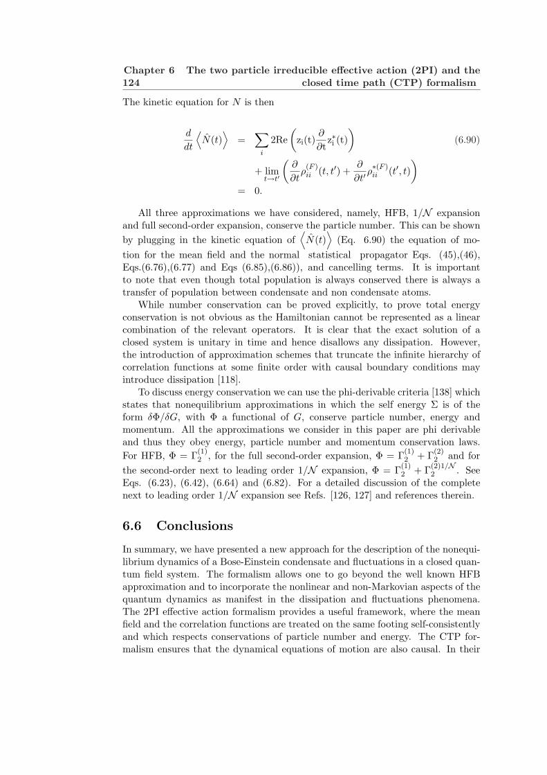
124Chapter 6 The two particle irreducible effective action (2PI) and the
closed time path (CTP) formalism
The kinetic equation for N is then
d
dt
⟨N(t)
⟩=
∑
i
2Re(
zi(t)∂
∂tz∗i (t)
)(6.90)
+ limt→t′
(∂
∂tρ(F )ii (t, t′) +
∂
∂t′ρ∗(F )ii (t′, t)
)
= 0.
All three approximations we have considered, namely, HFB, 1/N expansionand full second-order expansion, conserve the particle number. This can be shownby plugging in the kinetic equation of
⟨N(t)
⟩(Eq. 6.90) the equation of mo-
tion for the mean field and the normal statistical propagator Eqs. (45),(46),Eqs.(6.76),(6.77) and Eqs (6.85),(6.86)), and cancelling terms. It is importantto note that even though total population is always conserved there is always atransfer of population between condensate and non condensate atoms.
While number conservation can be proved explicitly, to prove total energyconservation is not obvious as the Hamiltonian cannot be represented as a linearcombination of the relevant operators. It is clear that the exact solution of aclosed system is unitary in time and hence disallows any dissipation. However,the introduction of approximation schemes that truncate the infinite hierarchy ofcorrelation functions at some finite order with causal boundary conditions mayintroduce dissipation [118].
To discuss energy conservation we can use the phi-derivable criteria [138] whichstates that nonequilibrium approximations in which the self energy Σ is of theform δΦ/δG, with Φ a functional of G, conserve particle number, energy andmomentum. All the approximations we consider in this paper are phi derivableand thus they obey energy, particle number and momentum conservation laws.For HFB, Φ = Γ(1)
2 , for the full second-order expansion, Φ = Γ(1)2 + Γ(2)
2 and forthe second-order next to leading order 1/N expansion, Φ = Γ(1)
2 + Γ(2)1/N2 . See
Eqs. (6.23), (6.42), (6.64) and (6.82). For a detailed discussion of the completenext to leading order 1/N expansion see Refs. [126, 127] and references therein.
6.6 Conclusions
In summary, we have presented a new approach for the description of the nonequi-librium dynamics of a Bose-Einstein condensate and fluctuations in a closed quan-tum field system. The formalism allows one to go beyond the well known HFBapproximation and to incorporate the nonlinear and non-Markovian aspects of thequantum dynamics as manifest in the dissipation and fluctuations phenomena.The 2PI effective action formalism provides a useful framework, where the meanfield and the correlation functions are treated on the same footing self-consistentlyand which respects conservations of particle number and energy. The CTP for-malism ensures that the dynamical equations of motion are also causal. In their

6.6 Conclusions 125
current form the scattering terms are nonlocal in time and thus hard to estimateanalytically, and their calculation is numerically demanding. However, this sys-tematic approach can be used as a quantitative means to obtain solutions in differ-ent regimes and make comparisons with kinetic theory results where a Markovianapproximation is assumed. We postpone these discussions to chapter 8.

126Chapter 6 The two particle irreducible effective action (2PI) and the
closed time path (CTP) formalism
Chapter 7
Nonequilibrium dynamics of apatterned loaded opticallattice: Beyond the mean fieldapproximation
In this chapter the two-particle irreducible (2PI) closed-time-path (CTP) effectiveaction formalism derived in chapter 6 is used to describe the nonequilibrium dy-namics of a Bose Einstein condensate (BEC) selectively loaded into every thirdsite of a one-dimensional optical lattice.
In chapter 4 we used a mean field approach to describe the dynamics of thissystem. However, we show here that even in the case when the kinetic energyis comparable to the interaction energy, interatomic collisions play a crucial rolein determining the quantum dynamics of the system, and therefore a mean fieldapproach is only accurate for short times. This result is demonstrated by com-parison between the mean field solutions and the exact numerical time evolutionof the initial state using the Bose Hubbard Hamiltonian for systems with smallnumbers of atoms (N ∼ 10) and lattice sites (M = 2 or 3). The exact numericalsolution is also used to test the validity of the various methods derived under the2PI-CTP approximation.
We show that because the second-order 2PI approximations include multi-particle scattering in a systematic way, they are able to capture damping effectsexhibited in the exact solution, which the mean field and the HFB approxima-tions fail to reproduce. However, our numerical results also show that all of theapproximations fail at late times, when interaction effects become significant.
7.1 Mean field dynamics
In this section we review the basic features of the mean field results obtained inchapter 4, in order to provide the context for the subsequent discussion of the
128Chapter 7 Nonequilibrium dynamics of a patterned loaded optical
lattice: Beyond the mean field approximation
dynamics in the 2PI-CTP formalism.
7.1.1 Dynamical evolution
By making the mean field ansatz in the Bose-Hubbard Hamiltonian, we replacethe field operator ai by a c-number zi(t). The amplitudes zi(t) satisfy the DNLSE(Eq. (4.6)).
In section 4.3.2, we treated a model case in which the initial occupancies of eachthird site are the same, and in which the condensate initially has a uniform phase.Thus at τ = 0, (τ ≡ tJ
~ ), the amplitudes zi(τ) are given by z3i(0) =√
3/M,z3i+1(0) = z3i+2(0) = 0, where M is the total number of lattice sites. For aninfinite lattice, or one with periodic boundary conditions, the amplitudes for allinitially occupied sites z3i(τ) = z0(τ) evolve identically in time, and the amplitudesfor the initially unoccupied sites satisfy z3i+1(τ) = z3i+2(τ) = for all τ . This allowsus to reduce the full set of equations to a set of two coupled equations for z0(τ)and z1(τ).
The solutions |z0(τ)| and |z1(τ)| are oscillatory functions whose amplitudesand common period, T (γ), are determined by the parameter γ ≡ 3NU
MJ = 3λ. Themean field dynamical behavior can be qualitatively divided into two regimes:
The tunneling dominated regime (γ < 1): In this regime the oscillationperiod is essentially constant, the role of interactions is relatively small, and theequations of motion are equivalent to those of a two-state Rabi problem. Thissystem will undergo Rabi oscillations whereby atoms periodically tunnel from theinitially occupied site into the two neighboring sites. For γ = 0 the period ofoscillation is 2π
3 .
Interaction dominated regime: The effect of interactions on the mean fielddynamics is to cause the energies of the initially occupied sites to shift relative tothose of the unoccupied sites. As γ increases the tunneling between sites occursat a higher frequency, but with reduced amplitude. The population of the ini-tially occupied sites becomes effectively self-trapped by the purely repulsive pairinteraction.
7.1.2 Comparisons with the exact solution
To check the validity of the mean field approximation, we made comparisons withthe exact many body solution for N = 6 atoms and M = 3 wells. We use amodest number of atoms and lattice sites for the comparisons, due to the fact thatthe Hilbert space needed for the calculations increases rapidly with the number ofatoms and wells.
7.1 Mean field dynamics 129
Exact solution
For the exact solution we used an initial state given by
|ϕ(0)〉 = (e−N/2e√
Na†o |0〉)⊗ |0〉 ⊗ |0〉 . (7.1)
The initial state represents a coherent state with an average of N atoms in theinitially populated well and zero atoms in the others. We chose this state becausein the experiment the loading of the atoms was done slow enough with respect toband excitations but fast with respect to many body excitations that at time t = 0most of the atoms in the initially populated wells were condensed.
The fully quantal solution was found by evolving the initial state in time withthe Bose-Hubbard Hamiltonian, so that |ϕ(t)〉 = e−
i~ Ht|ϕ(0)〉. To do the numerical
calculations we partitioned the Hilbert space in subspaces with a fixed numberof atoms and propagated independently the projections of the initial state on therespective subspaces. A subspace with Nn number of atoms and M wells is spannedby (Nn+M−1)!
Nn!(M−1)! states. This procedure could be done because the Hamiltonian
commutes with the number operator∑
i ai†ai, and therefore during the dynamics
the different subspaces never get mixed. The number of subspaces used for thenumerical evolution were such that no change in plots of the dynamical observableswas detected by adding another subspace. Generally for N atoms in the initialstate, this condition was achieved by including the subspaces between N − 4
√N
and N + 4√
N atoms.
Numerical comparisons
In Fig. 7.1 we plot the average population per well⟨a†i (t)ai (t)
⟩and the conden-
sate population per well |〈ai (t)〉|2 and compare them with the mean field predic-tions, i.e. |zi(t)|2, for three different values of γ. The salient features observed inthese comparisons are:
1. Weakly interacting regime (γ = 0.2):
In this regime the DNLSE gives a good description of the early time dy-namics. We observe in Fig. 7.1 that the total population per well predictedby the mean field solution agrees with the exact solution and also that thecondensate population remains large for the time under consideration. Weexpect the semiclassical approach to be valid for time scales less than theinverse energy level spacing. In Ref. [129] the authors show the validity ofthe semiclassical approach when τ < τcl ∼ N
Mγ in the case of two lattice sites.This time scale is in good agreement with the numerical results shown in inFig.7.1. After τcl quantum effects become important.
2. Intermediate regime (γ = 2):
Quantum fluctuations lead to a non-trivial modulation of the classical oscil-lations. In this regime the ratio between interaction and kinetic energy is
130Chapter 7 Nonequilibrium dynamics of a patterned loaded optical
lattice: Beyond the mean field approximation
small enough to allow the atoms to tunnel but not too small to make in-teraction effects negligible. Mean field results are accurate only for a shorttime. In this regime, the exact solution exhibits damped oscillations of theatomic population. Quantum scattering effects are crucial, even for ratherearly times.
To understand the dynamics in the weak and intermediate regimes, we haveto focus on the coherent properties of the system. Even though interactionscan be strong, the ground state is indeed superfluid. If we look at the initialcoherence of the system, determined by
⟨a†i (0)aj(0)
⟩i6=j
, it can be seen to
be zero due to the patterned loading. However, this is no longer the casefor t > 0 , and non-zero correlations are developed in the dynamics. Thedynamical restoration of the phase coherence which tends to distribute atomsuniformly among the lattice sites and to damp the oscillations characterizesthe dynamics in the superfluid regime. In Ref. [129], the authors show, notfor a patterned loaded initial state but for an initial Mott state also with zeroinitial phase coherence, how the phase coherence is restored dynamically.
3. Strongly correlated regime (γ = 12):
The system exhibits macroscopic quantum self-trapping of the population.Qualitatively, both the mean field and the exact solutions agree, in the sensethat both predict self-trapping of atoms in the initially populated wells, dueto interactions. However, the fast decrease of the condensate population andits subsequent revivals (as found in the exact solutions) give us an idea of theimportance of correlation effects beyond mean field. For a uniform loadedlattice, the collapse and revivals of the condensate in this strong interactingregime and the importance of quantum effects have been experimentallyobserved[47].
Even though there is minimal initial coherence between adjacent sites dueto the patterned loading procedure we are still preparing the system in asuperfluid state in the initially populated well. At time t = 0 we have acondensate fraction of order one. However, the ground state of the system isnot superfluid. It is expected then that, after some time, the phase is goingto randomize and this will lead to the collapse of the condensate population.After the collapse, the system will remain for a while with zero condensatepopulation. However, it can not remain zero forever because we are dealingwith a closed quantum system, with finite recurrence time. Therefore atsome time trev we expect the condensate to revive again. The collapses andrevivals of the condensate population in the strong interacting regime canbe easily estimated by considering the energy spectrum. In this regime theenergy eigenstates of the system are almost number (Fock) states and theenergy spectrum is almost quadratic, En ≈ n(n−1)U/2. The dynamics of thesystem is described by the interference of the different n-particle Fock statesthat span the coherent state of the initially populated well. At integer valuesof trev = (U/h)−1, the phase factors add to an integer value of 2π, leading

7.2 2PI-CTP approximations 131
to a revival of the initial state. This time scale agrees with the one estimatedin Ref.[130] for a more general situation. That reference, also shows how thecollapse time, tcoll, depends on the variance of the initial atomic distribution;it is given by: tcoll ∼ trev/(2πσ). If the initial state is a coherent state, theinitial distribution is Poissonian and tcoll is given by tcoll ∼ ~/(
√NU). For
the parameters used in the strongly correlated regime, γ = 12 and N = 6,we observe that the estimated collapses and revival times are in agreementwith what is shown in Fig. 7.1.
7.2 2PI-CTP approximations
It was shown in the previous section that to describe the dynamics of the patternedloaded optical lattice, approximations beyond the standard mean field theory arerequired. In this section we proceed to test the validity of the different 2PI-CTPapproximations derived in chapter 6, explicitly, the time dependent HFB approxi-mation, the full second-order approximation and the 1/N expansion up to second-order in the interaction strength. Because in all these approximations we useU/J as an expansion parameter we will focus our calculations on the intermediateregime, where the ratio U/J is small enough that truncation up to second-ordermakes sense but not too small so that interaction effects still have to be taken intoaccount.
We start by describing the initial conditions chosen for the numerical calcula-tions, then we outline the numerical algorithms used, and finally we discuss theresults.
7.2.1 Initial conditions and parameters
To model the patterned loading, the initial conditions assumed for the numericalsolutions were zi(0) = Nδi0, ρ
(F )ij (0, 0) = 1
2δij , ρ(ρ)ij (0, 0) = −iδij and m
(F )ij (0, 0)) =
m(ρ)ij (0, 0) = 0. Here zi(t) are the condensate amplitudes and ρ
(F )ij (ti, tj), ρ
(ρ)ij (ti, tj),
m(F )ij (ti, tj) and m
(ρ)ij (ti, tj) are the statistical and spectral normal and anomalous
propagators as defined in chapter 6. The initial conditions correspond to an initialcoherent state with N atoms in the initially populated well.
To study the kinetic energy dominated regime we chose for the simulationsthree different sets of parameters:. The first set is chosen to be in the very weakinteracting regime, M = 3, N = 6, J = 1 and U/J = 1/30. With this choice wewanted to show the validity of a mean field approach to describe this regime andthe corrections introduced by the higher order approximations. The second set ofparameters is M = 3, N = 8, J = 1 and U/J = 1/3. In this regime the kineticenergy is big enough to allow tunneling but the effect of the interactions is crucialin the dynamics.
At the mean field level (using the DNLSE) for a given number of wells, the onlyrelevant parameter for describing the dynamics of the system is the ratio UN/J .This is not the case in the exact solution where both UN/J and N are important.
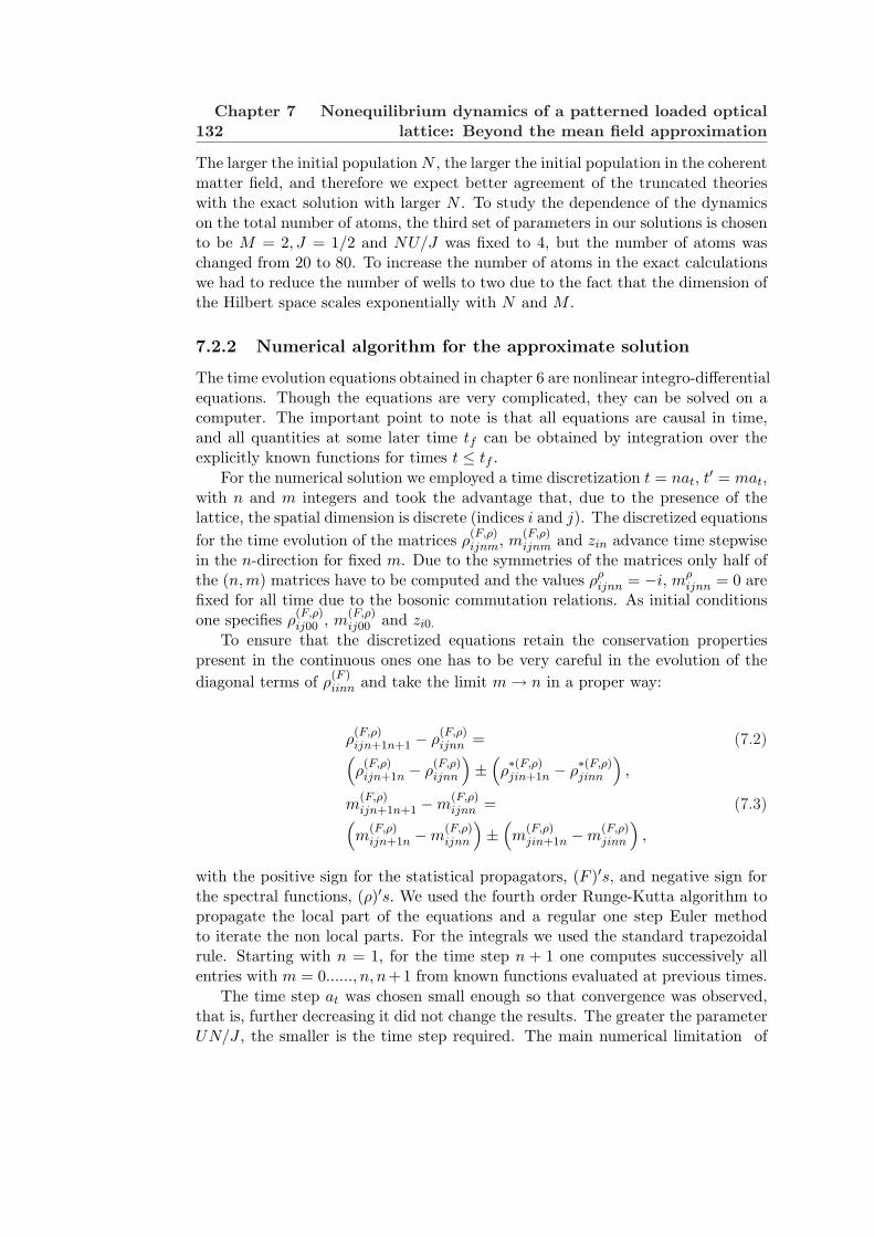
132Chapter 7 Nonequilibrium dynamics of a patterned loaded optical
lattice: Beyond the mean field approximation
The larger the initial population N , the larger the initial population in the coherentmatter field, and therefore we expect better agreement of the truncated theorieswith the exact solution with larger N . To study the dependence of the dynamicson the total number of atoms, the third set of parameters in our solutions is chosento be M = 2, J = 1/2 and NU/J was fixed to 4, but the number of atoms waschanged from 20 to 80. To increase the number of atoms in the exact calculationswe had to reduce the number of wells to two due to the fact that the dimension ofthe Hilbert space scales exponentially with N and M .
7.2.2 Numerical algorithm for the approximate solution
The time evolution equations obtained in chapter 6 are nonlinear integro-differentialequations. Though the equations are very complicated, they can be solved on acomputer. The important point to note is that all equations are causal in time,and all quantities at some later time tf can be obtained by integration over theexplicitly known functions for times t ≤ tf .
For the numerical solution we employed a time discretization t = nat, t′ = mat,with n and m integers and took the advantage that, due to the presence of thelattice, the spatial dimension is discrete (indices i and j). The discretized equationsfor the time evolution of the matrices ρ
(F,ρ)ijnm, m
(F,ρ)ijnm and zin advance time stepwise
in the n-direction for fixed m. Due to the symmetries of the matrices only half ofthe (n,m) matrices have to be computed and the values ρρ
ijnn = −i, mρijnn = 0 are
fixed for all time due to the bosonic commutation relations. As initial conditionsone specifies ρ
(F,ρ)ij00 , m
(F,ρ)ij00 and zi0.
To ensure that the discretized equations retain the conservation propertiespresent in the continuous ones one has to be very careful in the evolution of thediagonal terms of ρ
(F )iinn and take the limit m → n in a proper way:
ρ(F,ρ)ijn+1n+1 − ρ
(F,ρ)ijnn = (7.2)(
ρ(F,ρ)ijn+1n − ρ
(F,ρ)ijnn
)±
(ρ∗(F,ρ)jin+1n − ρ
∗(F,ρ)jinn
),
m(F,ρ)ijn+1n+1 −m
(F,ρ)ijnn = (7.3)(
m(F,ρ)ijn+1n −m
(F,ρ)ijnn
)±
(m
(F,ρ)jin+1n −m
(F,ρ)jinn
),
with the positive sign for the statistical propagators, (F )′s, and negative sign forthe spectral functions, (ρ)′s. We used the fourth order Runge-Kutta algorithm topropagate the local part of the equations and a regular one step Euler methodto iterate the non local parts. For the integrals we used the standard trapezoidalrule. Starting with n = 1, for the time step n + 1 one computes successively allentries with m = 0......, n, n+1 from known functions evaluated at previous times.
The time step at was chosen small enough so that convergence was observed,that is, further decreasing it did not change the results. The greater the parameterUN/J , the smaller is the time step required. The main numerical limitation of
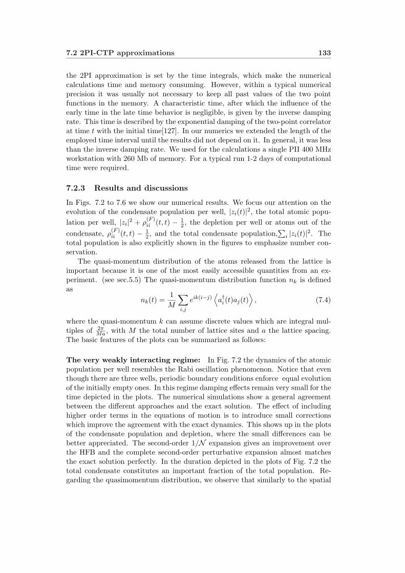
7.2 2PI-CTP approximations 133
the 2PI approximation is set by the time integrals, which make the numericalcalculations time and memory consuming. However, within a typical numericalprecision it was usually not necessary to keep all past values of the two pointfunctions in the memory. A characteristic time, after which the influence of theearly time in the late time behavior is negligible, is given by the inverse dampingrate. This time is described by the exponential damping of the two-point correlatorat time t with the initial time[127]. In our numerics we extended the length of theemployed time interval until the results did not depend on it. In general, it was lessthan the inverse damping rate. We used for the calculations a single PII 400 MHzworkstation with 260 Mb of memory. For a typical run 1-2 days of computationaltime were required.
7.2.3 Results and discussions
In Figs. 7.2 to 7.6 we show our numerical results. We focus our attention on theevolution of the condensate population per well, |zi(t)|2, the total atomic popu-lation per well, |zi|2 + ρ
(F )ii (t, t) − 1
2 , the depletion per well or atoms out of thecondensate, ρ
(F )ii (t, t) − 1
2 , and the total condensate population,∑
i |zi(t)|2. Thetotal population is also explicitly shown in the figures to emphasize number con-servation.
The quasi-momentum distribution of the atoms released from the lattice isimportant because it is one of the most easily accessible quantities from an ex-periment. (see sec.5.5) The quasi-momentum distribution function nk is definedas
nk(t) =1M
∑
i,j
eik(i−j)⟨a†i (t)aj(t)
⟩, (7.4)
where the quasi-momentum k can assume discrete values which are integral mul-tiples of 2π
Ma , with M the total number of lattice sites and a the lattice spacing.The basic features of the plots can be summarized as follows:
The very weakly interacting regime: In Fig. 7.2 the dynamics of the atomicpopulation per well resembles the Rabi oscillation phenomenon. Notice that eventhough there are three wells, periodic boundary conditions enforce equal evolutionof the initially empty ones. In this regime damping effects remain very small for thetime depicted in the plots. The numerical simulations show a general agreementbetween the different approaches and the exact solution. The effect of includinghigher order terms in the equations of motion is to introduce small correctionswhich improve the agreement with the exact dynamics. This shows up in the plotsof the condensate population and depletion, where the small differences can bebetter appreciated. The second-order 1/N expansion gives an improvement overthe HFB and the complete second-order perturbative expansion almost matchesthe exact solution perfectly. In the duration depicted in the plots of Fig. 7.2 thetotal condensate constitutes an important fraction of the total population. Re-garding the quasimomentum distribution, we observe that similarly to the spatial
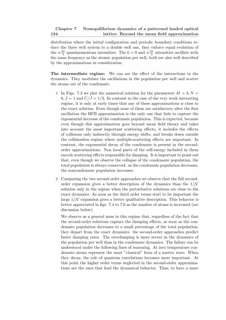
134Chapter 7 Nonequilibrium dynamics of a patterned loaded optical
lattice: Beyond the mean field approximation
distribution where the initial configuration and periodic boundary conditions re-duce the three well system to a double well one, they enforce equal evolution ofthe ±2π
3 quasimomentum intensities. The k = 0 and ±2π3 intensities oscillate with
the same frequency as the atomic population per well, both are also well describedby the approximations in consideration.
The intermediate regime: We can see the effect of the interactions in thedynamics. They modulate the oscillations in the population per well and scatterthe atoms out of the condensate.
1. In Figs. 7.3 we plot the numerical solution for the parameters M = 3, N =8, J = 1 and U/J = 1/3. In contrast to the case of the very weak interactingregime, it is only at early times that any of these approximations is close tothe exact solution. Even though none of them are satisfactory after the firstoscillation the HFB approximation is the only one that fails to capture theexponential decrease of the condensate population. This is expected, becauseeven though this approximation goes beyond mean field theory and takesinto account the most important scattering effects, it includes the effectsof collisions only indirectly through energy shifts, and breaks down outsidethe collisionless regime where multiple-scattering effects are important. Incontrast, the exponential decay of the condensate is present in the second-order approximations. Non local parts of the self-energy included in themencode scattering effects responsible for damping. It is important to point outthat, even though we observe the collapse of the condensate population, thetotal population is always conserved: as the condensate population decreases,the noncondensate population increases.
2. Comparing the two second-order approaches we observe that the full second-order expansion gives a better description of the dynamics than the 1/Nsolution only in the regime when the perturbative solutions are close to theexact dynamics. As soon as the third order terms start to be important thelarge 1/N expansion gives a better qualitative description. This behavior isbetter appreciated in figs. 7.4 to 7.6 as the number of atoms is increased (seediscussion below).
We observe as a general issue in this regime that, regardless of the fact thatthe second-order solutions capture the damping effects, as soon as the con-densate population decreases to a small percentage of the total population,they depart from the exact dynamics: the second-order approaches predictfaster damping rates. The overdamping is more severe in the dynamics ofthe population per well than in the condensate dynamics. The failure can beunderstood under the following lines of reasoning. At zero temperature con-densate atoms represent the most ”classical” form of a matter wave. Whenthey decay, the role of quantum correlations becomes more important. Atthis point the higher order terms neglected in the second-order approxima-tions are the ones that lead the dynamical behavior. Thus, to have a more
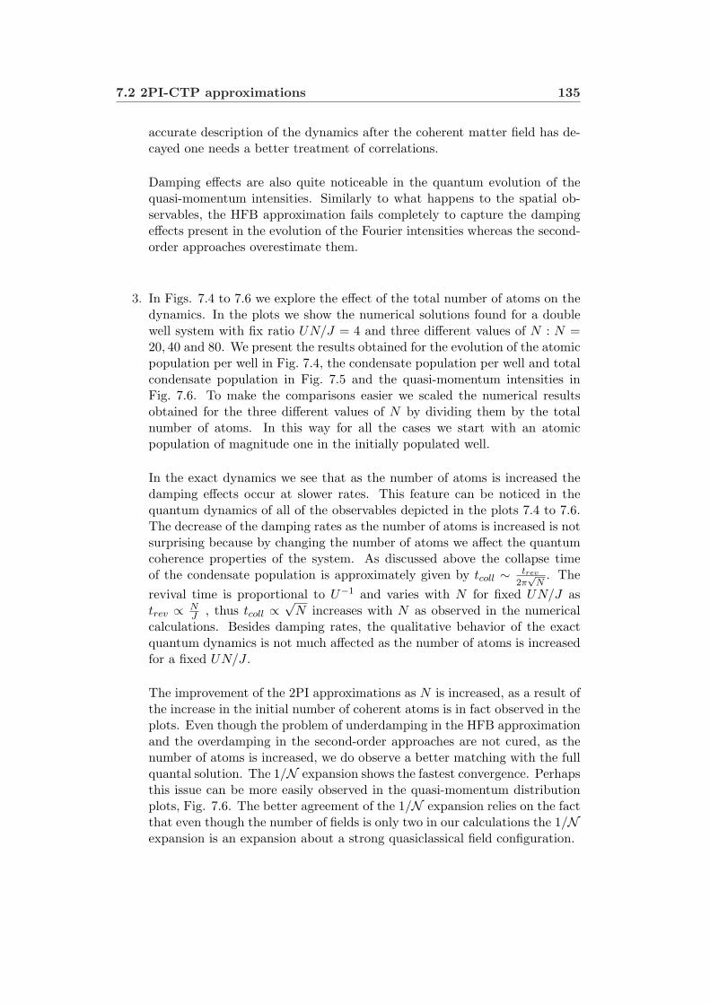
7.2 2PI-CTP approximations 135
accurate description of the dynamics after the coherent matter field has de-cayed one needs a better treatment of correlations.
Damping effects are also quite noticeable in the quantum evolution of thequasi-momentum intensities. Similarly to what happens to the spatial ob-servables, the HFB approximation fails completely to capture the dampingeffects present in the evolution of the Fourier intensities whereas the second-order approaches overestimate them.
3. In Figs. 7.4 to 7.6 we explore the effect of the total number of atoms on thedynamics. In the plots we show the numerical solutions found for a doublewell system with fix ratio UN/J = 4 and three different values of N : N =20, 40 and 80. We present the results obtained for the evolution of the atomicpopulation per well in Fig. 7.4, the condensate population per well and totalcondensate population in Fig. 7.5 and the quasi-momentum intensities inFig. 7.6. To make the comparisons easier we scaled the numerical resultsobtained for the three different values of N by dividing them by the totalnumber of atoms. In this way for all the cases we start with an atomicpopulation of magnitude one in the initially populated well.
In the exact dynamics we see that as the number of atoms is increased thedamping effects occur at slower rates. This feature can be noticed in thequantum dynamics of all of the observables depicted in the plots 7.4 to 7.6.The decrease of the damping rates as the number of atoms is increased is notsurprising because by changing the number of atoms we affect the quantumcoherence properties of the system. As discussed above the collapse timeof the condensate population is approximately given by tcoll ∼ trev
2π√
N. The
revival time is proportional to U−1 and varies with N for fixed UN/J astrev ∝ N
J , thus tcoll ∝√
N increases with N as observed in the numericalcalculations. Besides damping rates, the qualitative behavior of the exactquantum dynamics is not much affected as the number of atoms is increasedfor a fixed UN/J .
The improvement of the 2PI approximations as N is increased, as a result ofthe increase in the initial number of coherent atoms is in fact observed in theplots. Even though the problem of underdamping in the HFB approximationand the overdamping in the second-order approaches are not cured, as thenumber of atoms is increased, we do observe a better matching with the fullquantal solution. The 1/N expansion shows the fastest convergence. Perhapsthis issue can be more easily observed in the quasi-momentum distributionplots, Fig. 7.6. The better agreement of the 1/N expansion relies on the factthat even though the number of fields is only two in our calculations the 1/Nexpansion is an expansion about a strong quasiclassical field configuration.

136Chapter 7 Nonequilibrium dynamics of a patterned loaded optical
lattice: Beyond the mean field approximation
7.3 Conclusions
In this work we have used the CTP functional formalism for 2PI Green’s func-tions to describe the nonequilibrium dynamics of a condensate loaded in an opticallattice on every third lattice site. We have carried out the analysis up to second-order in the interaction strength.This approximation is introduced so as to makethe numerical solution manageable, but it is sufficient to account for dissipativeeffects due to multiparticle scattering that are crucial even at early times. Ourformulation is capable of capturing the salient features of the system dynamics inthe regime under consideration, such as the decay of the condensate populationand the damping of the oscillations of the quasi-momentum and population perwell unaccounted for in the HFB approximation. However, at the point wherean important fraction of the condensate population has been scattered out, thesecond-order approximations used here predict an overdamped dynamics. To im-prove on this a better treatment of higher correlations is required. One might tryto include the full next to leading order large N expansion without the truncationto second-order as done in Ref. [127] but it is not obvious that this will lead to therequired improvement. Alternatively, one may try to adopt a stochastic approach,but the challenge will be shifted to the derivation of a noise term (which is likelyto be both colored and multiplicative) which contains the effects of these highercorrelations and the solution of the stochastic equations.
Even though, as is clear that the second-order 2PI approximations fail to cap-ture the fully correlated dynamics in the system, it has been proved to work atintermediate times when correlations are not negligible and standard mean fieldtechniques fail poorly. Because of their success in describing moderately correlatedregimes, the second-order approximations could become a useful tool for describingother experimental situations.
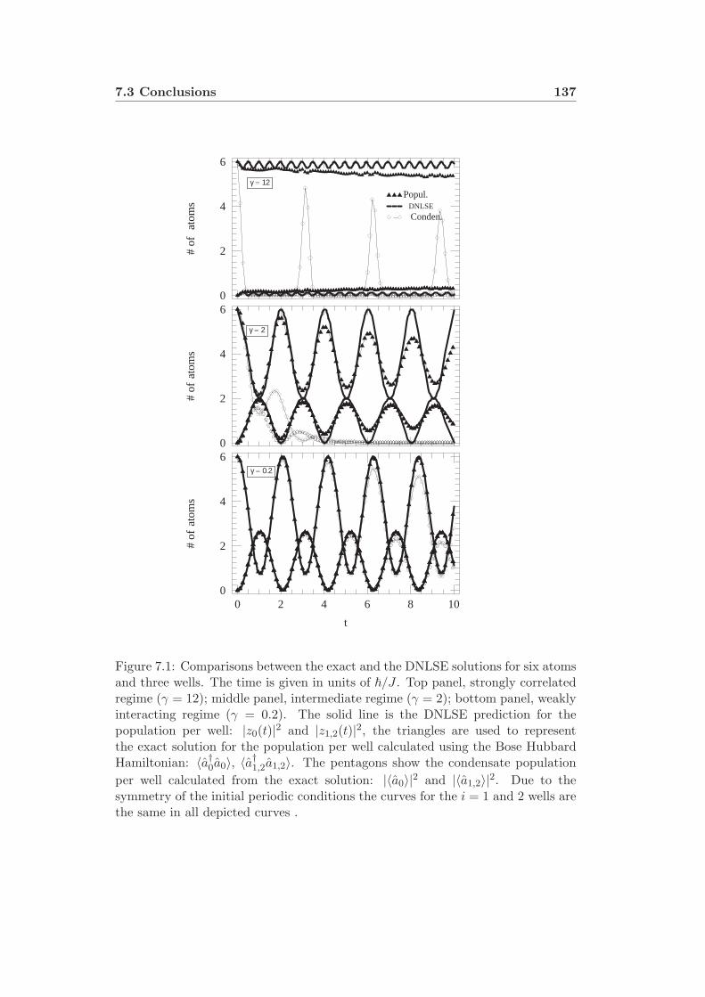
7.3 Conclusions 137
γ= 0.2
0 2 4 6 8 10
t
0
2
4
6
#of
atom
s
γ= 2
0
2
4
6
#of
atom
s
Conden.DNLSE
Popul.γ= 12
0
2
4
6
#of
atom
s
Figure 7.1: Comparisons between the exact and the DNLSE solutions for six atomsand three wells. The time is given in units of ~/J . Top panel, strongly correlatedregime (γ = 12); middle panel, intermediate regime (γ = 2); bottom panel, weaklyinteracting regime (γ = 0.2). The solid line is the DNLSE prediction for thepopulation per well: |z0(t)|2 and |z1,2(t)|2, the triangles are used to representthe exact solution for the population per well calculated using the Bose HubbardHamiltonian: 〈a†0a0〉, 〈a†1,2a1,2〉. The pentagons show the condensate populationper well calculated from the exact solution: |〈a0〉|2 and |〈a1,2〉|2. Due to thesymmetry of the initial periodic conditions the curves for the i = 1 and 2 wells arethe same in all depicted curves .

138Chapter 7 Nonequilibrium dynamics of a patterned loaded optical
lattice: Beyond the mean field approximation
0 2 4 6 8 10t
0
0.2
0.4
0.6
0.8
Dep
letio
n/w
ell
0 2 4 6 8 10t
1.9
1.95
2
2.05
mom
entu
m
0
2
4
6
Popu
latio
n/w
ell
0
2
4
6
cond
ensa
te/w
ell
5
5.5
6
Tot
alC
onde
nsat
e
HFB1/N2ndExact
5
5.25
5.5
5.75
6
Tot
alN
umbe
rFigure 7.2: Comparisons between the exact solution(solid line), the HFB approxi-mation (boxes), the second-order large N approximation (pentagons) and the full2PI second-order approximation(crosses) for the very weak interacting regime. Theparameters used were M = 3, N = 6, J = 1 and U/J = 1/30. The time is givenin units of ~/J . In the plots where the population, condensate and depletion perwell are depicted the top curves correspond to the initially populated well solutionsand the lower to the initially empty wells. Notice the different scale used in thedepletion plot. In the momentum distribution plot the upper curve correspondsto the k = ±2π/3 intensities and the lower one to the k = 0 quasi-momentumintensity.
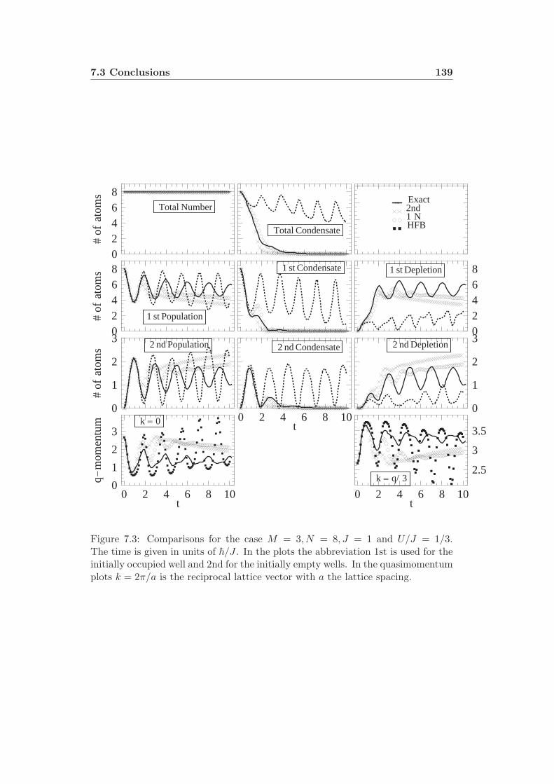
7.3 Conclusions 139
k = 0
0 2 4 6 8 10t
0
1
2
3
q-m
omen
tum
k = q/ 3
0 2 4 6 8 10t
2.5
3
3.5
2 nd Population
0
1
2
3
#of
atom
s 2 nd Condensate
0 2 4 6 8 10t
2 nd Depletion
0
1
2
3
1 st Population
02468
#of
atom
s 1 st Condensate 1 st Depletion
02468
Total Number
02468
#of
atom
s
Total Condensate HFB1N2ndExact
Figure 7.3: Comparisons for the case M = 3, N = 8, J = 1 and U/J = 1/3.The time is given in units of ~/J . In the plots the abbreviation 1st is used for theinitially occupied well and 2nd for the initially empty wells. In the quasimomentumplots k = 2π/a is the reciprocal lattice vector with a the lattice spacing.
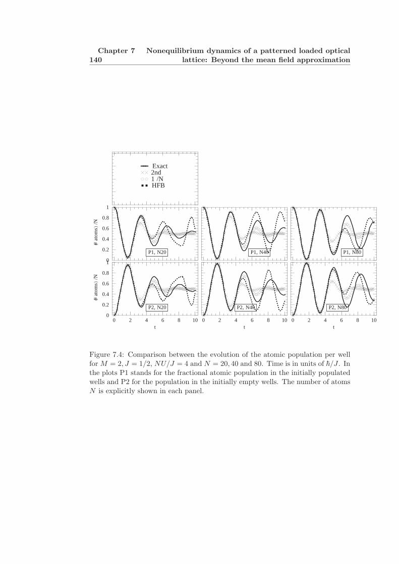
140Chapter 7 Nonequilibrium dynamics of a patterned loaded optical
lattice: Beyond the mean field approximation
P2, N20
0 2 4 6 8 10t
0
0.2
0.4
0.6
0.8
1
(#at
oms)/
N
P2, N40
0 2 4 6 8 10t
P2, N80
0 2 4 6 8 10t
P1, N20
0
0.2
0.4
0.6
0.8
1
(#at
oms)/
N
P1, N40 P1, N80
HFB1/N2ndExact
Figure 7.4: Comparison between the evolution of the atomic population per wellfor M = 2, J = 1/2, NU/J = 4 and N = 20, 40 and 80. Time is in units of ~/J . Inthe plots P1 stands for the fractional atomic population in the initially populatedwells and P2 for the population in the initially empty wells. The number of atomsN is explicitly shown in each panel.

7.3 Conclusions 141
CT, N20
0 2 4 6 8 10t
0
0.2
0.4
0.6
0.8
1
(#at
oms)/
N
CT, N40
0 2 4 6 8 10t
CT, N80
0 2 4 6 8 10t
C2, N20
0
0.2
0.4
0.6
0.8
1
(#at
oms)/
N
C2, N40 C2, N80
C1, N20
0
0.2
0.4
0.6
0.8
1
(#at
oms)/
N
C1, N40C1, N80
HFB1/N2ndExact
Figure 7.5: Time evolution of the condensate population per well and the totalcondensate population,for the same parameters as Fig. 7.4. Time is in units of~/J . In the plots C1 stands for the fractional condensate population in the initiallypopulated well, C2 for the fractional condensate population in the initially emptyone and CT for the total condensate fraction.

142Chapter 7 Nonequilibrium dynamics of a patterned loaded optical
lattice: Beyond the mean field approximation
ko, N20
0 2 4 6 8 10t
0.2
0.3
0.4
0.5
0.6
0.7
q-m
omen
tum ko, N40
0 2 4 6 8 10t
ko, N80
0 2 4 6 8 10t
k1, N20
0.3
0.4
0.5
0.6
0.7
0.8
q-m
omen
tum
k1, N40 k1, N80
HFB1N2ndExact
Figure 7.6: Dynamical evolution of the quasi-momentum intensities. The param-eters used were M = 2, J = 1/2, NU/J = 4 and N = 20, 40 and 80. Time isin units of ~/J . In the plots ko denotes the k = 0 quasi-momentum componentand k1 the k = π/a one (a the lattice spacing). The plots are scaled to set theintegrated quasi-momentum density to one for all N .
Chapter 8
From the 2PI-CTPapproximations to kinetictheories and local equilibriumsolutions
In chapter 6 we used the CTP functional formalism for 2PI Green’s functionsto derive dynamical equations of motion. We have carried out the analysis upto second-order in the interaction strength. In chapter 7 we used the formalismto investigate the nonequilibrium dynamics of a condensate loaded on every thirdsite of an optical lattice. We showed that the formalism allowed us to go beyondthe HFB approximation and to incorporate the nonlinear and non-Markovian as-pects of the quantum dynamics as manifested in the dissipation and fluctuationphenomena.
However, in the present form the equations of motion are complicated nonlocalnonlinear equations from which we can hardly get any physical information regard-ing the system behavior except by numerical solution. Moreover, the numericalsolutions are complicated enough that application to real system with many latticesites are presently beyond the scope of standard computation capabilities. Never-theless, when the perturbation induces disturbances in the system of wave lengthlonger than thermal wave lengths and frequencies much smaller than characteristicparticle energies then the system is in a regime where standard kinetic theoriesgive a good description of the dynamics. The purpose of this chapter is then tosimplify the complicated 2PI-CTP equations and show that they in fact reproduce,in the slowly varying regime, standard kinetic theories and equilibrium solutionsfor weakly interacting gases well known in the literature since the late 1950’s.
144Chapter 8 From the 2PI-CTP approximations to kinetic theories and
local equilibrium solutions
8.1 Rewriting the 2PI-CTP second-order equations
In order to make the comparisons with standard approaches we will start by gettingrid of the matrix indices that were useful to derive the equations of motion butwhich complicate the notation. We define the quantities
z(ti) ≡ zai (t), (8.1)
G(ti, t′j) ≡ −iGijab(t, t
′), (8.2)H(ti, t′j) ≡ −iza
i (t)zjb(t′), (8.3)
G>(ti, t′j) ≡ −iG>ij
a
c(t, t′), (8.4)
G<(ti, t′j) ≡ −iG<ij
a
c(t, t′) = −iG>
jic
a(t′, t). (8.5)
Here we used the notation introduced in Eqs. (6.26) and (6.27). With these defini-tions we now explicitly separate the single particle, the HFB and the second-ordercontributions in the equations of motion for the condensate and the propagators(Eq. (6.22) and Eq. (6.24)).
∑
k
∫dt′′
(D−1
o (ti, t′′k)− SHFB(ti, t′′k))z (t′′k) =
∑
k
∫dt′′S(ti, t′′k)z(t
′′k),(8.6)
∑
k
∫dt′′
(D−1
o (ti, t′′k)− ΣHFB(ti, t′′k))G(t′′k, t
′j) =
∑
k
∫dt′′Σ(ti, t′′k)G(t′′k, t
′j)
−δijδC(t− t′), (8.7)
where D−1o (ti, t′j) is the inverse free particle propagator given by:
D−1o (ti, t′j) ≡ (iδijσz∂t + J(δi+1j + δi−1j)− δijVi) δ(t− t′), (8.8)
with σ being the Pauli matrices:
σz =(
1 00 −1
), σx =
(0 11 0
). (8.9)
In D−1o (ti, t′j) we have allowed the presence of an external potential Vi. The label
HFB stands for the HFB contribution. Using the definition (8.1)-(8.5) in Eqs.(6.43) and (6.45) they can then be rewritten as:
ΣHFB(ti, t′j) ≡ (8.10)
iU
N(Tr
(H(ti, t′j) + G(ti, t′j)
)I + 2
(H(ti, t′j) + G(ti, t′j)
))δ(t− t′)δij,,
SHFB(ti, t′j) ≡ iU
N(Tr
(H(ti, t′j)I + G(ti, t′j)
)+ 2G(ti, t′j)
)δ(t− t′)δij . (8.11)
8.1 Rewriting the 2PI-CTP second-order equations 145
where I is the identity matrix. To evaluate the second-order contribution, we useEqs. (6.31) and (6.32) but instead of setting the initial time to zero we choose it tobe −∞ and in this way we recover the standard Kadanoff and Baym integrationcontours [137]:
∑
k
∫ ∞
−∞dt′′
(D−1
o (ti, t′′k)− SHFB(ti, t′′k))H(t′′k, t
′j)−
∫ t
−∞dt′′γ(ti, t′′k)H(t′′k, t
′j)
= 0, (8.12)∑
k
∫ ∞
−∞dt′′H(ti, t′′k)
(D−1
o (t′′k, t′j)− SHFB(t′′k, t
′j)
)+
∫ t
−∞dt′′H(ti, t′′k)γ(t′′k, t
′j)
= 0, (8.13)
∑
k
∫ ∞
−∞dt′′
(D−1
o (ti, t′′k)− ΣHFB(ti, t′′k))G(≷)(t′′k, t
′j) = (8.14)
∑
k
∫ t
−∞dt′′Γ(ti, t′′k)G
(≷)(t′′k, t′j)−
∑
k
∫ t′
−∞dt′′Σ(≷)(ti, t′′k)A(t′′k, t
′j),
∑
k
∫ ∞
−∞dt′′G(≷)(ti, t′′k)
(D−1
o (t′′k, t′j)− ΣHFB(t′′k, t
′j)
)= (8.15)
∑
k
∫ t
−∞dt′′A(ti, t′′k)Σ
(≷)(t′′k, t′j)−
∑
k
∫ t′
−∞dt′′G(≷)(ti, t′′k)Γ(t′′k, t
′j).
In the above equations, Eq. (8.15) is the hermitian conjugate of Eq. (8.14), Eq.(8.13) is the hermitian conjugate of Eq. (8.12) and we have introduced the spectralfunctions
γ(ti, t′j) ≡ (S>(ti, t′j)− S<(ti, t′j)), (8.16)Γ(ti, t′′j ) ≡ (Σ>(ti, t′′j )− Σ<(ti, t′′j )), (8.17)A(ti, t′′j ) ≡ (G>(ti, t′′j )−G<(ti, t′′j )). (8.18)
Notice that A(ti, t′′j ) is just the spectral function defined in Eq.(6.34) multipliedby a minus sign, however, we adopted the notation γ, Γ and A to be consistentwith standard Kadanoff and Baym notation [137].
If we use the full second-order expansion, Eqs.(6.71 and 6.72), it can be shownthat the matrices S(≷) and Σ(≷) are given by
S(≷)(ti, t′j) ≡ −12
(2U
N)2 [
G(≷)(ti, t′j)Tr(G(≷)(ti, t′j)G
(≶)(t′j , ti))
+ 2G(≷)(ti, t′j)G(≶)(t′j , ti)G
(≷)(ti, t′j)], (8.19)

146Chapter 8 From the 2PI-CTP approximations to kinetic theories and
local equilibrium solutions
Σ(≷)(ti, t′j) ≡ −12
(2U
N)2
× (8.20)
H(ti, t′j)Tr(G(≷)(ti, t′j)G
(≶)ik (t′j , ti)
)+ 2H(ti, t′j)G
(≶)(t′j , ti)G(≷)(ti, t′j)
+2G(≷)(ti, t′j)(H(t′j , ti)G
(≷)(ti, t′j) + G(≶)(t′j , ti)H(ti, t′j) + G(≶)(t′j , ti)G(≷)(ti, t′j)
)
G(≷)(ti, t′j)Tr(H(t′j , ti)G
(≷)(ti, t′j) + G(≶)(t′j , ti)H(ti, t′j) + G(≶)(t′j , ti)G(≷)(ti, t′j)
).
It is convenient to decompose the above equations in their matrix components.To do that we introduce the definitions
G>(ti, t′j) = −i
(ρij mij
m∗ji ρji
), (8.21)
G<(ti, t′j) = −i
(ρij mji
m∗ij ρji
). (8.22)
Using Eqs. (8.21) and (8.22) into the self-energy equations we get
ΣHFB(ti, t′j) =2U
N(
2|zi|2 + ρii + ρii z2i + mii
z∗2i + m∗ii 2|zi|2 + ρii + ρii
)δ(t− t′)δij ,(8.23)
SHFB(ti, t′j) =2U
N( |zi|2 + ρii + ρii mii
m∗ii |zi|2 + ρii + ρii
)δ(t− t′)δij , (8.24)
S>11(ti, t
′j) =
−i8U2
N 2ρij(2mijm
∗ji + ρijρji), (8.25)
S>12(ti, t
′j) =
−i8U2
N 2mij(mijm
∗ji + 2ρijρji), (8.26)
S<11(ti, t
′j) =
−i8U2
N 2ρij(2mjim
∗ij + ρjiρij), (8.27)
S<12(ti, t
′j) =
−i8U2
N 2mji(mijm
∗ji + 2ρjiρij), (8.28)
8.2 Boltzmann equations 147
Σ>11(ti, t
′j) =
−i8U2
N 2(ρjiρ
2ij + 2mij ρijmji
∗ + 2ρijmji∗zizj + (8.29)
ρ2ijzjzi
∗ + 2ρjiρijzizj∗ + 2mijmji
∗zj∗zi + 2mij ρijzi
∗zj∗),
Σ>12(ti, t
′j) =
−i8U2
N 2(2ρjimij ρij + 2ρjiρijzizj + mij
2mji∗ + (8.30)
2mijzizjmji∗ + 2mij ρijzjzi
∗ + 2ρjimijzizj∗ + mij
2zi∗zj
∗),
Σ<11(ti, t
′j) =
−i8U2
N 2(ρij
2ρji + 2ρijmjimij∗ + 2ρijzizjmij
∗ + ρ2ijzjzi
∗ +
2ρij ρjizizj∗ + 2mjizimij
∗zj∗ + 2ρijmjizi
∗zj∗), (8.31)
Σ<12(ti, t
′j) =
−i8U2
N 2(2ρijmjiρji + 2ρij ρjizizj + mji
2mij∗ + (8.32)
2mjizizjmij∗ + 2ρijmjizjzi
∗ + 2mjiρjizizj∗ + mji
2zi∗zj
∗),
and
S(≷)22 (ti, t′j) = S
(≷)11 (ti, t′j) ρij 7→ ρij , (8.33)
S(≷)21 (ti, t′j) = S
(≷)12 (ti, t′j) mji 7→ mij
∗ , (8.34)
Σ(≷)22 (ti, t′j) = Σ(≷)
11 (ti, t′j) zi 7→ zj , ρij 7→ ρij , (8.35)
Σ(≷)21 (ti, t′j) = Σ(≷)
12 (ti, t′j) zi 7→ zj∗,mji 7→ mij
∗ . (8.36)
The above expressions for the self-energy exactly agree with the ones used in Refs.[59, 60, 62]. In Refs. [59, 62] the authors used these equations as their startingpoint before applying the Markovian approximation.
8.2 Boltzmann equations
From previous sections it can be observed that the equations of motion at second-order are quite involved: they are nonlinear and nonlocal integro differential equa-tions, not readily solvable in closed form. To progress further we need to introduceapproximations based on physical considerations. One of them is to recognize twotime scales in the system, one related to quantum processes (microscopic) whichdetermines the degree of quantum-mechanical entanglement of the system and onerelated to the statistical and kinetic behavior (macroscopic) determined by therange of the interactions among particles. In a classical point of view the twodifferent scales in the system can be understood as the time (or length) scale sep-aration between the duration of a collision event (or scattering length) and theinverse collision rate (or the mean free path). Close to equilibrium (when the ex-ternal potential induces disturbances much longer than the lattice spacing andfrequencies much smaller than the characteristic particle energies) and in theweakly interacting regime, we expect that a reasonable assumption would be toconsider the kinetic scale larger than the quantum one, which in a classical picturecorresponds to assume that be the time between collisions (or mean free path) islong compared to the reaction time (or scattering length).

148Chapter 8 From the 2PI-CTP approximations to kinetic theories and
local equilibrium solutions
Using this approximation it is possible to recast the quantum dynamics into themuch simpler forms of kinetic theory. In contrast to normal systems were there isnot a condensate, in condensed systems making the scale separation requires firstto do a gauge transformation which makes it easier to identify (and coarse-grainaway) the fast variations induced by the rapid change of the condensate phase.Following Ref. [139] we introduce the gauge transformation
zi(t) = eiθi(t)√
no(ti), (8.37)G(≷)(ti, t′j) = eiθi(t)σzG(≷)(ti, t′j)e
−iθj(t′)σz , (8.38)
where√
no(ti) and θi(t) are real. In equilibrium, ∆θi ≡ (θi+1/2 − θi−1/2)/a isrelated to the superfluid velocity and the time derivative of the phase to thechemical potential. Extending these identifications to the nonequilibrium systemwe define the chemical potential and superfluid velocity as
µi = −~∂tθi − ~2
4Ja2vsi2 − Vi, (8.39)
~vsi = 2J∆θia
2. (8.40)
After the gauge transformation the variables no, G , vs and µ are expected to beslowly varying functions of
R = (i + j)/2, T = (t + t′)/2, (8.41)
and peaked about the zeros of
r = (i− j), τ = (t− t′), (8.42)
necessary conditions to derive Boltzmann-type kinetic equations.The equations of motion are invariant under the phase transformation if we
replace D−1o by D−1
o :
D−1o (ti, t′j) = (~δij(iσz∂t − ∂tθi)− δijVi+ (8.43)
J(eiσz∆θi+1/2δi+1j + e−iσz∆θi−1/2δi−1j))
δ(t− t′).
Since hereafter we will use the gauge-transformed functions exclusively, in thefollowing the tildes will be dropped to simplify the notation. To obtain the kineticequations we Fourier transform the functions G and no with respect to r and τ .The Fourier transform reads
G(≷)(ti, t′j) = G(≷)
((T +
τ
2
)R+r/2
,(T − τ
2
)R−r/2
)
≡ −i1
2πM
∑q
∫dωe(iqr−iωτ)G(≷)(Rq; T, ω), (8.44)
H(ti, t′j) = H
((T +
τ
2
)R+r/2
,(T − τ
2
)R−r/2
)
≡ −i1
2πM
∑q
∫dωe(iqr−iωτ)H(Rq; T, ω), (8.45)
8.2 Boltzmann equations 149
Neglecting second-order variations of no(Rq;T, ω) we can approximate it as
H(Rq; T, ω) = 2πM (I + σx) no(R, T )δ(ω)δq0. (8.46)
In Eq.(8.46), the quantity no(R, T ) is just related to the condensate density ofatoms at the space time point (Ra, T ). In Eq.(8.44), the two-point functionG
(<)11 (Rq; T, ω) corresponds to the well known Wigner distribution function [140]. It
can be interpreted as the density of noncondensed particles with quasimomentum q
and energy ~ω at the lattice site R and time T . On the other hand, G(>)11 (Rq; T, ω)
is essentially the density of states available to a particle that is added to the systemat (Ra, T ) with quasimomentum q and energy ~ω. As opposed to a normal system,the presence of the condensate gives non zero values to the off diagonal terms ofthe functions G
(≷)12 (Rq; T, ω). We refer to them as the anomalous contributions to
the respective two point functions.The generalized Boltzmann equations can be obtained as the Fourier transform
of the equations of motion for the case in which the variations in R and T are veryslow. In particular when the inverse propagator D−1
o and the self energies vary verylittle as Ra is changed by a characteristic excitation wavelength or T is changedby an inverse excitation energy. Following Ref.[139] and assuming a (q, ω, R, T )dependence of the variables, which is not explicitly written for simplicity, we getthe following equations:
(D−1
o −<S +i
2γ
)H = − i
2[D−1
o ,H]+
i
2[<S, H] +
14
[γ,H] , (8.47)
H
(D−1
o −<S − i
2γ
)= − i
2[H, D−1
o
]+
i
2[H,<S]− 1
4[H, γ] , (8.48)
(D−1
o −<Σ +i
2Γ)
G(≷) − Σ(≷)
(<G +
i
2A
)= − i
2
[D−1
o , G(≷)]
+i
2
[<Σ, G(≷)
]+
i
2
[Σ(≷),<G
]+
14
[Γ, G(≷)
]− 1
4
[Σ(≷), A
], (8.49)
G(≷)
(D−1
o −<Σ− i
2Γ)
−(<G− i
2A
)Σ(≷) = − i
2
[G(≷), D−1
o
]+
i
2
[G(≷),<Σ
]+
i
2
[<G,Σ(≷)
]− 1
4
[G(≷), Γ
]+
14
[A, Σ(≷)
], (8.50)
with
D−1o (Rq;T, ω) ≡ (σz (~ω − vs2J sin(qa)) + (2J cos(qa) + µR(T )) I) . (8.51)
Because all the quantities are slowly varying functions of R and T , in Eqs (8.47-8.50) we approximated the discretized equation to continuous differential equa-tions. The brackets denote the generalized Poisson brackets defined as:
[A,B] =∂A
∂ω
∂B
∂T− ∂A
∂T
∂B
∂ω+ ∂RA∂qB − ∂qA∂RB. (8.52)
150Chapter 8 From the 2PI-CTP approximations to kinetic theories and
local equilibrium solutions
In the equations we have also introduced the following functions:
<S(Rq; T, ω) = SHF (Rq; T, ω) + <SB(Rq;T, ω), (8.53)<Σ(Rq; T, ω) = ΣHF (Rq; T, ω) + <ΣB(Rq;T, ω), (8.54)
<SB(Rq; T, ω) = P
∫dω′
2π
γ(Rq; T, ω)ω − ω′
, (8.55)
<ΣB(Rq; T, ω) = P
∫dω′
2π
Γ(qR, ω′)ω − ω′
, (8.56)
<G = P
∫dω′
2π
A(Rq; T, ω)ω − ω′
. (8.57)
with P denoting the Cauchy principal value and γ(Rq;T, ω), Γ(Rq; T, ω), SHF (Rq;T, ω),ΣHF (Rq;T, ω) and A(Rq; T, ω) understood as Fourier transforms of the functionsγ(ti, t′j), Γ(ti, t′j), S
HF(ti, t′j), ΣHF (ti, t′j) and A(ti, t′j) respectively.
If we define the statistical variables as:
F =G> + G<
2, (8.58)
Π =Σ> + Σ<
2. (8.59)
Eq. (8.49)and Eq. (8.50), can be rewritten in term of statistical and spectralfunctions as:
(D−1
o −<Σ +i
2Γ)
F − Π(<G +
i
2A
)= (8.60)
− i
2
[D−1
o −<Σ +i
2Γ, F
]−
[Π,<G +
i
2A
],
F
(D−1
o −<Σ− i
2Γ)
−(<G− i
2A
)Π = (8.61)
− i
2
[F, D−1
o −<Σ− i
2Γ]−
[<G− i
2A,Π
],
(D−1
o −<Σ)A− Γ<G = − i
2[
D−1o −<Σ, A
]− [Γ,<G]
, (8.62)
A(D−1
o −<Σ)−<GΓ = − i
2[
A,D−1o −<Σ
]− [<G,Γ]
. (8.63)
Eqs. (8.47), (8.48) and (8.60)- (8.63) are our passage to the Boltzmann equa-tions. They describe the state of the gas at a given time. In contrast to the HFBequations, they include collisional integrals to describe binary interactions.
To progress further we can introduce even more simplifications based on phys-ical assumptions. The ordinary Boltzmann equation emerges from the approxima-tion in which the self energies that appear on the left side of Eqs.(8.47), (8.48) and
8.2 Boltzmann equations 151
(8.60)- (8.63) are handled differently from those which appear on the right. Thesetwo appearances of the self-energy play a different physical role in the descrip-tion of the dynamics [137]. The self energies on the right hand side describe thedynamical effects of collisions, i.e., how the collisions transfer particles from oneenergy-momenta configuration to another. On the other hand, the self energies onthe left describe the quantum kinetic effects due to interactions, i.e. how inter-action effects change the energy momentum dispersion relations from that of freeparticles to a more complicated spectrum. Because these two effects are physicallyso different, we can treat the left and the right hand sides in different ways.
In the derivation of the ordinary Boltzmann equations, one completely neglectsall the kinetic effects in the second-order self energies (the dependence on T and Rin the second-order self energy terms on the right hand side) and retain dynamicaleffects (T and R dependence on the left hand side). In this way, we get the familiarBoltzmann equations which describe the particles as free particles in between col-lisions. This is a reasonable assumption in dilute weakly interacting gases in whichthe duration of a collision is very short compared to the essentially interaction-freedynamics between isolated collisions. Neglecting kinetic effects in the second-orderself energies, Eqs.(8.47), (8.48) and (8.60)-(8.63) can be approximated to
(D−1
o −<S +i
2γ
)H = − i
2[D−1
o − SHF ,H], (8.64)
H
(D−1
o −<S − i
2γ
)= − i
2[H, D−1
o − SHF], (8.65)
(D−1
o −<Σ +i
2Γ)
F −Π(<G +
i
2A
)= − i
2[D−1
o − ΣHF , F], (8.66)
(D−1
o −<Σ)A− Γ<G = − i
2[D−1
o − ΣHF , A], (8.67)
F
(D−1
o −<Σ− i
2Γ)−
(<G− i
2A
)Π = − i
2[F, D−1
o − ΣHF], (8.68)
A(D−1
o −<Σ)−<GΓ = − i
2[A,D−1
o − ΣHF]. (8.69)
If we take the trace of the sum and the difference of each one of the above equationswith its hermitian conjugate, they can be simplified to :
Tr(
D−1o −<S
)H
= 0, (8.70)
Tr(
D−1o −<Σ
)F −Π<G
= 0, (8.71)
Tr(
D−1o −<Σ
)A− Γ<G
= 0, (8.72)
Tr[D−1
o − SHF ,H]
= −Tr(γH), (8.73)
Tr[D−1
o − ΣHF , F]
= −Tr(ΓF −ΠA). (8.74)
Tr[D−1
o − ΣHF , A]
= 0 (8.75)

152Chapter 8 From the 2PI-CTP approximations to kinetic theories and
local equilibrium solutions
Moreover, if we define the operator krM = M12 + M∗21 and apply it again to
the sum and the difference of each one of the equations (8.60) to (8.63) with itstranspose we also get:
Re(kr
(D−1
o −<S)H
)=
12Im
(kr
[D−1
o − SHF,H]+ k(γH)
), (8.76)
Re(kr
(D−1
o −<Σ)F−Π<G
)=
12Im
(kr
[D−1
o − ΣHF, F]+ kr(ΓF−ΠA)
),(8.77)
Re(kr
(D−1
o −<Σ)A− Γ<G
)=
12Im
(kr
[D−1
o − ΣHF, A])
, (8.78)
Im(kr
(D−1
o −<S)H
)= −1
2Re
(kr
[D−1
o − SHF,H]+ k(γH)
), (8.79)
Im(kr
(D−1
o −<Σ)F−Π<G
)= −1
2Re
(kr
[D−1
o − ΣHF, F]+ kr(ΓF−ΠA)
),(8.80)
Im(kr
(D−1
o −<Σ)A− Γ<G
)= −1
2Re
(kr
[D−1
o − ΣHF, A])
, (8.81)
with Re and Im denoting the real and imaginary parts. To close this set of equa-tions we need an equation of motion for the superfluid velocity which can be foundfrom the definitions Eq.(8.39) and Eq.(8.40) to be:
~2Ja2
∂vs
∂T= − ∂
∂R
((µ + V ) +
~4Ja2
vs2
). (8.82)
Eqs.(8.70-8.81) together with Eq.(8.82) form a closed set of equations thatdescribe the state of the gas at a given time. Equations (8.70-8.72) and (8.76-8.78) are usually called gap equations. They describe the quantum properties ofthe gas which is evolving according to the Boltmaznn equations (8.73-8.75) and(8.79-8.81). Under the derived formalism the Boltzmann and gap equations forma coupled set of equations which replaces the original dynamics. The equationshave to be solved self consistently for any analysis.
8.3 Equilibrium properties for a homogeneous system
In this section we will show how the nonequilibrium Boltzmann equations lead, ina special case, to the linear equilibrium solutions discussed in chapter 5 upgradedwith second-order corrections in U not included in the quadratic approximations.There are two situations in which we expect an equilibrium solution to come fromthe Boltzmann equations. Firstly, when the system has never been disturbed itremains in its equilibrium state. Secondly, when the system has had sufficient timeto relax after an applied perturbation.
At equilibrium, in the absence of any external potential, the functions G≷ andH are completely independent of R and T . In this case the generalized Poissonbrakets terms are zero and Eqs.(8.72, 8.75) and (8.78, 8.75) imply that:
A(D−1
o −<Σ)− (<G)Γ = 0. (8.83)
8.3 Equilibrium properties for a homogeneous system 153
Because <G(q, ω) is determined by A(q, ω) as indicated in Eq. (8.57), Eq. (8.83)is satisfied when A(q, ω) is given by
A(q, ω) = i
[D−1
o −<S +i
2Γ]−1
−[D−1
o −<S − i
2Γ]−1
, (8.84)
and the function <G(q, ω) given by
<G(q, ω) = P
∫dω′
2π
A(q, ω′)ω − ω′
=12
[D−1
o −<S +i
2Γ]−1
+[D−1
o −<S − i
2Γ]−1
. (8.85)
From Eqs.(8.73), (8.79),(8.74) and (8.80)) we also get that at equilibrium
γ = 0, (8.86)ΓF −ΠA = 0. (8.87)
Eqs. (8.86) and (8.87) are just the mathematical statement of detailed balance.They just represent the physical condition that at equilibrium the net rate ofchange of the density of particles with momentum q and energy ω is zero. Sinceit is always possible to write [137]
F (q, ω) =(
nq(ω) +12
)A(q, ω), (8.88)
then Eq.(8.87) can only be satisfied if
Π(q, ω) =(
nq(ω) +12
)Γ(q, ω), (8.89)
is satisfied. Detailed study of the structure of the self energy indicates that nq(ω)is related to the Bose-Einstein distribution, nq(ω) = 1
eβ~ω−1with β interpreted as
the local inverse temperature in energy units [137, 139].Since H contains delta functions in momentum and energy at equilibrium, we getfrom Eq. (8.70):
µ = −2J + <S11(0, 0) + <S12(0, 0). (8.90)
8.3.1 Quasiparticle formalism
In the non interacting case the diagonal terms of A(q, ω) are just delta functionswith peaks at values of ~ω that matches the possible energy difference which re-sults from adding a single particle with quasimomentum q to the system. In the
154Chapter 8 From the 2PI-CTP approximations to kinetic theories and
local equilibrium solutions
many body system the energy spectrum is sufficiently complex so that the diag-onal elements of A(q, ω) are not delta functions but instead continuous functionsof ω. However, there are always sharp peaks in A. These sharp peaks representthe coherent and long lived excitations, which behave like weakly interacting par-ticles. These excitations are called quasiparticles. From Eq. (8.84) it is possibleto see that the quasiparticle decay rate is determined by Γ. The quasiparticleapproximation is obtained by considering Γ very small for small values of ω. Thisassumption implies that D−1 ≡ D−1
o − <Σ − i2Γ is essentially real with only an
infinitesimal imaginary part. The zeros of D−1 about which A is very sharplypeaked are identified with the quasiparticle energies ~ωq.Using the assumption of a very small Γ, and the identity limε→0
1ω−ω′+iε = P 1
ω−ω′−iπδ(ω − ω′), it is possible to write the matrix components of D−1 as:
D−1(q, ω) = ~ω(
1 00 −1
)−
( Lqq(q, ω) Mq−q(q, ω)M∗
q−q(q, ω) L∗qq(−q,−ω)
), (8.91)
with
Lqq(ω) = −2J cos qa− µ + ΣHFB11 (q, ω) +
∫dω′
2π
Γ11(q, ω′)ω − ω′ + iε
, (8.92)
Mq−q(ω) = ΣHFB12 (q, ω) +
∫dω′
2π
Γ12(q, ω′)ω − ω′ + iε
. (8.93)
The quasiparticle amplitudes uq and vq are the solutions to the eigenvalue problem( Lqq(q, ωq) Mq−q(q, ωq)M∗
q−q(q, ωq) L∗qq(−q,−ωq)
)(uq
vq
)= ~ωq
(1 00 −1
)(uq
vq
), (8.94)
and satisfy the normalization condition |uq|2−|vq|2 = 1. In the absence of vorticesit is always possible to find an ensemble in which the amplitudes (uq, vq) arepurely real and uq = u−q, vq = v−q. In terms of the quasiparticle amplitudes,the matrix elements of the spectral function A, Eq.(8.84), are given by:
A11(q, ω) = −2Im
[u2
q
ω − ωq + i0+− v2
q
ω − ωq + i0−
]
= 2π[u2
qδ(ω − ωq)− v2qδ(ω + ωq)
], (8.95)
A12(q, ω) = 2Im[
uqvq
ω − ωq + i0+− vquq
ω − ωq + i0−
]
= −2πuqvq [δ(ω − ωq)− δ(ω + ωq)] , (8.96)A22(q, ω) = −A11(−q,−ω), (8.97)A21(q, ω) = A∗12(q, ω). (8.98)
Finally, using the definitions of F and A, we can express the matrix compo-nents: ρq(ω), ρq(ω) and mq(ω) defined as the Fourier transform of ρij , ρij and mij
respectively (see Eqs. (8.21) and (8.22)) in terms of quasiparticle amplitudes:
8.3 Equilibrium properties for a homogeneous system 155
ρq(ω) = 2π[u2
qnq(ω)δ(ω − ωq) + v2q (1 + nq(ω))δ(ω + ωq)
], (8.99)
ρq(ω) = 2π[u2
q(1 + nq)(ω)δ(ω − ωq) + v2qnq(ω)δ(ω + ωq)
], (8.100)
mq(ω) = 2πuqvq [nq(ω)δ(ω − ωq)− (1 + nq(ω))δ(ω + ωq)] . (8.101)
8.3.2 HFB approximation
Under the HFB approximation the matrix <Σ and <S are just given by ΣHFB
and SHFB. In terms of the quasiparticle amplitudes and setting N = 2, they canbe written as:
ΣHFB = U
(2 (no + n) no + mno + m 2 (no + n)
), (8.102)
SHFB = U
(no + 2n m
m no + 2n
). (8.103)
with
n = =1M
∑q
(1 + nq(ωq))v2q + u2
qnq, (8.104)
m =1M
∑q
uqvq (2nq(ωq) + 1) . (8.105)
In the HFB approximation, Eq.(8.94) and Eq. ( 8.90) then yield:
( −2J cos(qa)− µ + 2U(no + n) U (no + m)U (no + m) −2J cos(qa)− µ + 2U(no + n)
)(uq
vq
)= ~ωq
(uq
−vq
),
(8.106)
µ = −2J + Uno + 2Un + Um. (8.107)
As a final step, to fix the total density to n, the constraint
n = no + n, (8.108)
has to be satisfied.For a given density and temperature Eqs. (8.106)- (8.108) form a closed set
of equations. At zero temperature, they reduce to the HFB equations derived inchapter 5 using the quadratic approximation.
156Chapter 8 From the 2PI-CTP approximations to kinetic theories and
local equilibrium solutions
8.3.3 Second-order and Beliaev approximations
When second-order terms are taking into account the matrixes Lqq and Mq−q
become energy dependent. For simplicity we restrict the calculations to the zerotemperature case when nq = 0. In terms of the quasiparticle amplitudes thecontributions to the self-energy at second-order are given by
Mq−q(q, ω) = Uno + Um +2U2
M~no
∑
k
(2AkBq−k + 2CkAp + 2CkBq−k + 3CkCq−k
ω − ωk − ωq−k + iε
−2BkAq−k + 2CkAp + 2CkBq−k + 3CkCq−k
ω + ωk + ωq−k − iε
)(8.109)
+2U2
M2~∑
k,p
(2AkBpCq−k−p + CkCpCq−k−p
ω − ωk − ωp − ωq−k−p + iε− 2BkApCq−k−p + CkCpCq−k−p
ω + ωk + ωp + ωq−k−p − iε
),
Lqq(q, ω) = −2J cos qa− µ + 2Uno + 2Un +2U2no
~M∑
k
(AkAq−k + 2AkBq−k + 4CkAq−k + 2CkCq−k
ω − ωk − ωq−k + iε
− BkBq−k + 2(BkAq−k) + 4CkBq−k + 2CkCq−k
ω + ωk + ωq−k − iε
)(8.110)
+2U2
~M2
∑
k,p
(AkApBq−k−p + 2AkCpCq−k−p
ω − ωk − ωp − ωq−k−p + iε
)−
(BkBpAq−k−p + 2BkCpCq−k−p
ω + ωk + ωp + ωq−k−p − iε
),
µ = −2J + Uno + 2Un + Um (8.111)
− 2U2
~M2
∑
k,p
(2AkBpCk+p + 2BkApCk+p + 2CkCpCk+p
ωk + ωp + ωk+p
)
− 2U2
~M2
∑
k,p
(2AkCpCk+p +AkApBk+p + 2BkCpCk+p + BkBpAk+p
ωk + ωp + ωk+p
),
where the quantities A, B and C are defined as
Ak = u2k, Bk = v2
k, Ck = −ukvk. (8.112)
The inclusion of second-order terms modifies the structure of the HFB equa-tions. The matrix that we need to diagonalize to find the quasiparticle energiesdepends now on the quasiparticle mode in consideration. This means that a sep-arate nonlinear problem must be solved for every quasiparticle state, whereas thesolution of the HFB equations yields the whole quasiparticle spectrum. The ma-trix which is to be diagonalized also become intrinsically non-local and to solvefor a quasiparticle state with quasimomentum q we have to sum over all different

8.3 Equilibrium properties for a homogeneous system 157
quasimomenta. Finally, the diagonal elements are no longer equal as was alwaysthe case in all the quadratic approximations considered in chapter 5.
If we omit the second-order terms containing no condensate amplitudes, theequations that we get are the tight-binding version of the ones originally derivedby Beliaev [63]:
Mq−q(q, ω) = Uno + Um +2U2
~Mno
∑
k
(2AkBq−k + 2CkAp + 2CkBq−k + 3CkCq−k
ω − ωk − ωq−k + iε
− 2BkAq−k + 2CkAp + 2CkBq−k + 3CkCq−k
ω + ωk + ωq−k − iε
), (8.113)
Lqq(q, ω) = 4J sin2(qa/2) + Uno − Um + (8.114)2U2no
~M∑
k
(AkAq−k + 2AkBq−k + 4CkAq−k + 2CkCq−k
ω − ωk − ωq−k + iε
− BkBq−k + 2(BkAq−k) + 4CkBq−k + 2CkCq−k
ω + ωk + ωq−k − iε
), (8.115)
µ = −2J + Uno + 2Un + Um. (8.116)
As discussed in chapter 5, the HFB approximation has the problem that it isnot gapless. It was shown by Beliaev that when second-order Beliaev contributionsare included the gap problem disappears. The reason is that as m introduces themany-body scattering matrix in the off-diagonal terms, second-order correctionsintroduce the many-body scattering matrix in the diagonal terms. This can be seenby considering the second-order Beliaev corrections in the particle approximation,uq → 1, vq → 0. In this case the second-order terms in Eq.(8.115) become
L(2)qq (q, ω) = −2U2no
~M∑
k
1ω − ωk − ωq−k − iε
. (8.117)
Comparison with Eq. (5.121) shows that L(2)qq (q, ω) is the second order contribution
to the many body scattering matrix.When both HFB and second-order corrections are included the quasiparticle
energies not only are shifted with respect to the BdG quasiparticle energies butthey also become complex. The imaginary part that the quasiparticle energiesacquire comes from the poles of the second-order terms and it is associated witha damping rate. The physical meaning is that when the energy denominator inthe second-order terms vanishes a real decay process is energetically allowed. Thedamping mechanism in which a quasiparticle decay into two of lower energy isknown as Beliaev damping and was calculated by Beliaev in the case of a uniformBose superfluid [63].

158Chapter 8 From the 2PI-CTP approximations to kinetic theories and
local equilibrium solutions
8.4 Conclusions
In summary, we showed in this chapter that the complicated non local non Marko-vian second-order solutions derived under the 2PI-CTP formalism, actually reduceto the standard kinetic theory solutions when the scale separation assumption ismade. We also showed that at equilibrium the full second-order 2PI equations re-produce the second-order corrections to the self energy well known since Beliaev.
Chapter 9
Characterizing the MottInsulator Phase
Besides the superfluid regime, the other regime where analytic solutions becomerelatively simple is the Mott insulator phase. Deep in the Mott insulator regimethe kinetic energy term in the Hamiltonian, which delocalizes the atoms, can betreated as a perturbation. In this chapter we use perturbation theory to describethe basic properties of the Mott phase. We study both a translationally invariantsystem when no other external potential is present and the case when there isan external harmonic confinement, as is the case in real experimental situations.Specifically, the trapped system is studied assuming a parameter regime wheremulti-occupancy in inhibited which is the relevant regime for the lattice basedquantum computation proposals.
9.1 Commensurate translationally invariant case
9.1.1 Perturbation theory
In this section we assume a commensurately filled one dimensional lattice withinteger filling factor N/M = g, periodic boundary conditions and a parameterregime where U/J À (U/J)c with (U/J)c the critical point, so that we are deepin the insulating phase. In this parameter regime, it is fair to consider the kineticterm of Bose-Hubbard Hamiltonian as a perturbation:
H = H(0) + δH, (9.1)
H(0) =12U
∑n
a†na†nanan, (9.2)
δH = −J∑
n
(a†n an+1 + a†n+1 an ). (9.3)
The unperturbed Hamiltonian includes only the on-site interaction term, whichis diagonal in a number Fock state basis, and to zeroth order the ground state

160 Chapter 9 Characterizing the Mott Insulator Phase
|Φ0〉 is the Fock state with g atoms in every lattice site. We refer to this stateas the target state |T 〉. The lowest lying excitations are described by the Fockstates, |Ψnm〉, that have g + 1 particles at site n, g − 1 particles at site m, andexactly g particles in every other site. We call these states one particle-hole (1-ph)excitations . There are M(M−1) 1-ph excitations and because of the translationalsymmetry of the system they are degenerate at zeroth order. All of them have anenergy U above the ground state. This energy gap is one of the most importantcharacteristics of the Mott insulator phase.
∣∣∣Φ(0)0
⟩≡ |T 〉 ≡ |g, g, ...., g, g〉 , (9.4)
∣∣∣Φ(0)i
⟩≡ |Ψnm〉n 6=m i = 1, . . . , M(M − 1) (9.5)
=
∣∣∣∣∣∣g, ..., g + 1︸ ︷︷ ︸
n
, ..., g − 1︸ ︷︷ ︸m
, .., g
⟩.
The unperturbed energies are
E(0)0 =
U
2Mg(g − 1), (9.6)
E(0)i = U + E
(0)0 i = 1, . . . , M(M − 1). (9.7)
At first order the kinetic energy term mixes the target state with 1-ph excita-tions with the particle and the hole at adjacent sites. The first order ground statewave-function is
∣∣∣Φ(1)0
⟩=
(|T 〉+
J
U
√2Mg(g + 1)|S〉
), (9.8)
with |S〉 the normalized translationally invariant state with a particle and hole atadjacent sites:
|S〉 ≡M∑
n=1
|Ψnn+1〉+ |Ψnn−1〉√2M
. (9.9)
Notice the factor M that appears in the first order correction. It gives a restrictionon the validity of a perturbative treatment as the number of lattice sites increases.In order for perturbation theory to be valid, the parameter Jg
U
√M has to be small.
The first order correction to the ground state energy vanishes. The second ordercorrection is given by
E(2)0 = −2J2M
Ug(g + 1). (9.10)
Because of the degeneracy of the unperturbed states, in order to find first ordercorrections to the M(M−1) low lying excited states we must diagonalize the kinetic
9.1 Commensurate translationally invariant case 161
energy Hamiltonian within the 1-ph subspace. If we span the eigenstates as a linearcombinations of 1-ph excitations,
∣∣∣Φ(1)i
⟩=
M∑
n,m=1,m6=n
Cinm |Ψnm〉 , (9.11)
the necessary and sufficient conditions that the coefficients Cinm have to fulfill in
order to diagonalize the kinetic energy operator are given by the following equations
−(g + 1)(Cin+1m + Ci
n−1m)− g(Cinm+1 + Ci
nm−1) = EiCinm, (9.12)
with E(1)i = U − JEi. Besides Eq. (9.12), the amplitudes have to fulfill two other
equations:
Cinn = 0, (9.13)
Cin+Mm = Ci
nm+M = Cinm. (9.14)
Eq. (9.12) is analogous to the tight-binding Schrodinger equation of a two dimen-sional square lattice in the x − y plane, with the x direction associated with theposition of the extra particle and the y direction with the position of the hole. Thedifferent weights g + 1 and g can be understood in the 2D-lattice model as differ-ent effective masses in the two directions. Eq. (9.14) imposes periodic boundaryconditions, whereas the constraint Ci
nn = 0 takes into account the requirementthat the extra particle and the hole at the same site annihilate each other. It canbe thought of as a hard wall in the x = y axis. The solutions are not straightfor-ward due to the fact that the effective mass difference breaks the lattice symmetryaround the x = y axis and makes the hard wall constraint hard to fulfill.
We now describe a procedure for solving the eigenvalue equations and evalu-ating limiting cases where it is possible to find analytic solutions. Without anyconstraint, a general solution of Eq. (9.12) has the form
Cnm ∝ einzeimt, (9.15)
withEi = −2 ((g + 1) cos (z) + g cos (t)) . (9.16)
To satisfy the constraint Cnn = 0 we use the linear character of the problem andlook for a linear combination of solutions which have the same eigenvalue Ei butwhich also fulfill the hard wall constraint. We look then for a general solution ofthe form:
Cnm ∝ sin (r(n−m)) eimleins, (9.17)
and determine the free parameters, l, r, s by forcing the solution to satisfy Eq.(9.12). This procedure leads to the following equation:
(g + 1) cos (r + s) + g cos (l − r) = (g + 1) cos (s− r) + g cos (l + r) . (9.18)
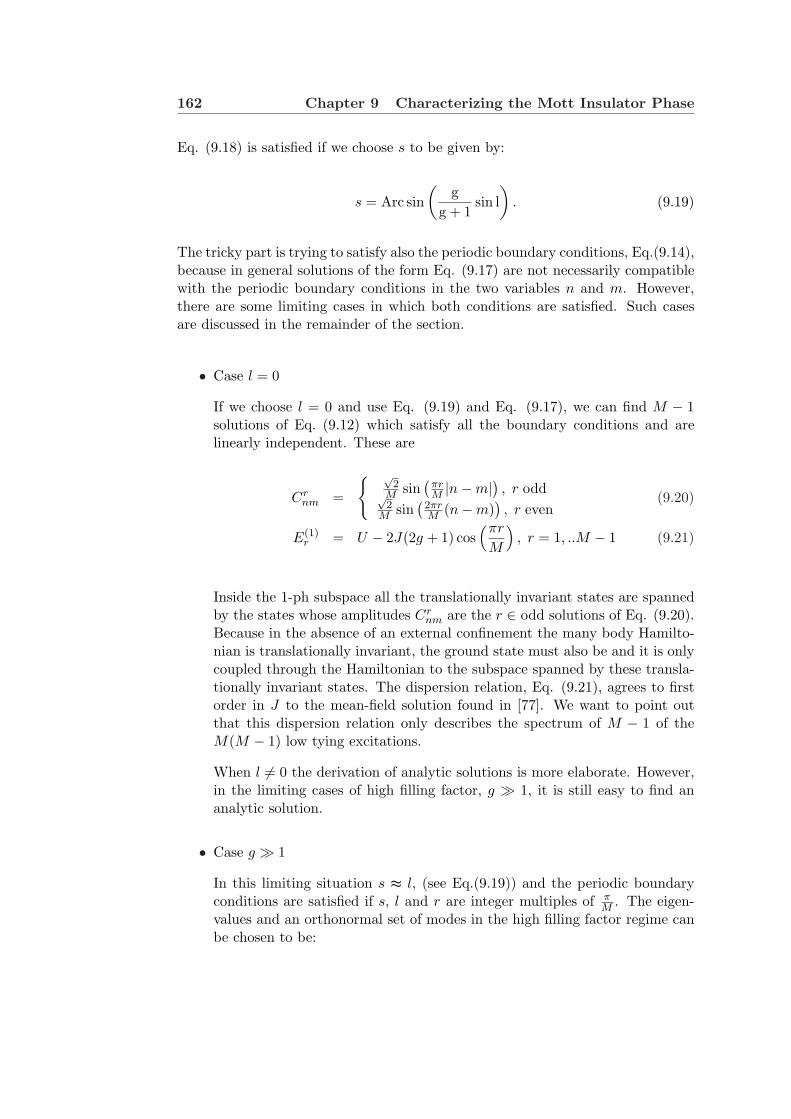
162 Chapter 9 Characterizing the Mott Insulator Phase
Eq. (9.18) is satisfied if we choose s to be given by:
s = Arc sin(
gg + 1
sin l)
. (9.19)
The tricky part is trying to satisfy also the periodic boundary conditions, Eq.(9.14),because in general solutions of the form Eq. (9.17) are not necessarily compatiblewith the periodic boundary conditions in the two variables n and m. However,there are some limiting cases in which both conditions are satisfied. Such casesare discussed in the remainder of the section.
• Case l = 0
If we choose l = 0 and use Eq. (9.19) and Eq. (9.17), we can find M − 1solutions of Eq. (9.12) which satisfy all the boundary conditions and arelinearly independent. These are
Crnm =
√2
M sin(
πrM |n−m|) , r odd√
2M sin
(2πrM (n−m)
), r even
(9.20)
E(1)r = U − 2J(2g + 1) cos
(πr
M
), r = 1, ..M − 1 (9.21)
Inside the 1-ph subspace all the translationally invariant states are spannedby the states whose amplitudes Cr
nm are the r ∈ odd solutions of Eq. (9.20).Because in the absence of an external confinement the many body Hamilto-nian is translationally invariant, the ground state must also be and it is onlycoupled through the Hamiltonian to the subspace spanned by these transla-tionally invariant states. The dispersion relation, Eq. (9.21), agrees to firstorder in J to the mean-field solution found in [77]. We want to point outthat this dispersion relation only describes the spectrum of M − 1 of theM(M − 1) low tying excitations.
When l 6= 0 the derivation of analytic solutions is more elaborate. However,in the limiting cases of high filling factor, g À 1, it is still easy to find ananalytic solution.
• Case g À 1
In this limiting situation s ≈ l, (see Eq.(9.19)) and the periodic boundaryconditions are satisfied if s, l and r are integer multiples of π
M . The eigen-values and an orthonormal set of modes in the high filling factor regime canbe chosen to be:
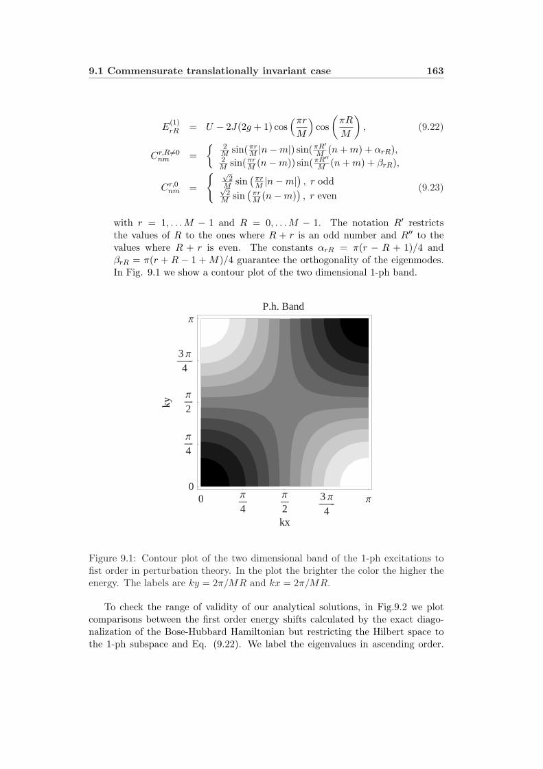
9.1 Commensurate translationally invariant case 163
E(1)rR = U − 2J(2g + 1) cos
(πr
M
)cos
(πR
M
), (9.22)
Cr,R 6=0nm =
2M sin(πr
M |n−m|) sin(πR′M (n + m) + αrR),
2M sin(πr
M (n−m)) sin(πR′′M (n + m) + βrR),
Cr,0nm =
√2
M sin(
πrM |n−m|) , r odd√
2M sin
(πrM (n−m)
), r even
(9.23)
with r = 1, . . . M − 1 and R = 0, . . .M − 1. The notation R′ restrictsthe values of R to the ones where R + r is an odd number and R′′ to thevalues where R + r is even. The constants αrR = π(r − R + 1)/4 andβrR = π(r + R − 1 + M)/4 guarantee the orthogonality of the eigenmodes.In Fig. 9.1 we show a contour plot of the two dimensional 1-ph band.
0 Π
4Π
23 Π
4Π
kx
0
Π
4
Π
2
3 Π
4
Π
ky
P.h. Band
Figure 9.1: Contour plot of the two dimensional band of the 1-ph excitations tofist order in perturbation theory. In the plot the brighter the color the higher theenergy. The labels are ky = 2π/MR and kx = 2π/MR.
To check the range of validity of our analytical solutions, in Fig.9.2 we plotcomparisons between the first order energy shifts calculated by the exact diago-nalization of the Bose-Hubbard Hamiltonian but restricting the Hilbert space tothe 1-ph subspace and Eq. (9.22). We label the eigenvalues in ascending order.
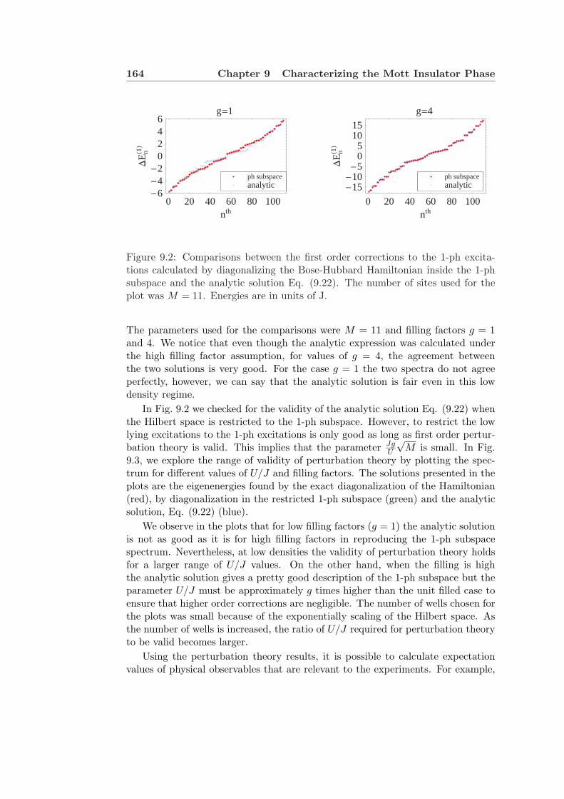
164 Chapter 9 Characterizing the Mott Insulator Phase
0 20 40 60 80 100nth
-6-4-2
0246
DE
nH1L
g=1
analyticph subspace
0 20 40 60 80 100nth
-15-10-5
05
1015
DE
nH1L
g=4
analyticph subspace
Figure 9.2: Comparisons between the first order corrections to the 1-ph excita-tions calculated by diagonalizing the Bose-Hubbard Hamiltonian inside the 1-phsubspace and the analytic solution Eq. (9.22). The number of sites used for theplot was M = 11. Energies are in units of J.
The parameters used for the comparisons were M = 11 and filling factors g = 1and 4. We notice that even though the analytic expression was calculated underthe high filling factor assumption, for values of g = 4, the agreement betweenthe two solutions is very good. For the case g = 1 the two spectra do not agreeperfectly, however, we can say that the analytic solution is fair even in this lowdensity regime.
In Fig. 9.2 we checked for the validity of the analytic solution Eq. (9.22) whenthe Hilbert space is restricted to the 1-ph subspace. However, to restrict the lowlying excitations to the 1-ph excitations is only good as long as first order pertur-bation theory is valid. This implies that the parameter Jg
U
√M is small. In Fig.
9.3, we explore the range of validity of perturbation theory by plotting the spec-trum for different values of U/J and filling factors. The solutions presented in theplots are the eigenenergies found by the exact diagonalization of the Hamiltonian(red), by diagonalization in the restricted 1-ph subspace (green) and the analyticsolution, Eq. (9.22) (blue).
We observe in the plots that for low filling factors (g = 1) the analytic solutionis not as good as it is for high filling factors in reproducing the 1-ph subspacespectrum. Nevertheless, at low densities the validity of perturbation theory holdsfor a larger range of U/J values. On the other hand, when the filling is highthe analytic solution gives a pretty good description of the 1-ph subspace but theparameter U/J must be approximately g times higher than the unit filled case toensure that higher order corrections are negligible. The number of wells chosen forthe plots was small because of the exponentially scaling of the Hilbert space. Asthe number of wells is increased, the ratio of U/J required for perturbation theoryto be valid becomes larger.
Using the perturbation theory results, it is possible to calculate expectationvalues of physical observables that are relevant to the experiments. For example,
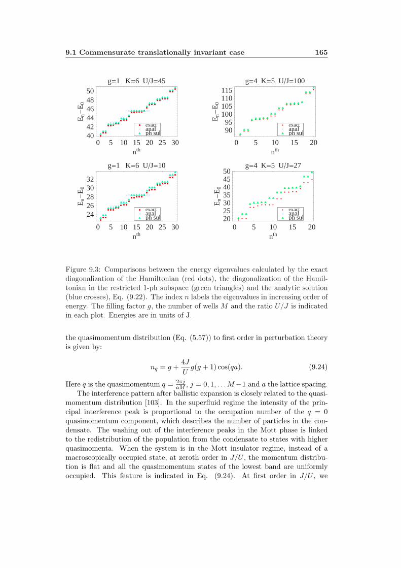
9.1 Commensurate translationally invariant case 165
0 5 10 15 20 25 30nth
2426283032
En-
E0
g=1 K=6 UJ=10
ph subanalexact
0 5 10 15 20nth
20253035404550
En-
E0
g=4 K=5 UJ=27
ph subanalexact
0 5 10 15 20 25 30nth
404244464850
En-
E0
g=1 K=6 UJ=45
ph subanalexact
0 5 10 15 20nth
9095
100105110115
En-
E0
g=4 K=5 UJ=100
ph subanalexact
Figure 9.3: Comparisons between the energy eigenvalues calculated by the exactdiagonalization of the Hamiltonian (red dots), the diagonalization of the Hamil-tonian in the restricted 1-ph subspace (green triangles) and the analytic solution(blue crosses), Eq. (9.22). The index n labels the eigenvalues in increasing order ofenergy. The filling factor g, the number of wells M and the ratio U/J is indicatedin each plot. Energies are in units of J.
the quasimomentum distribution (Eq. (5.57)) to first order in perturbation theoryis given by:
nq = g +4J
Ug(g + 1) cos(qa). (9.24)
Here q is the quasimomentum q = 2πjaM , j = 0, 1, . . . M−1 and a the lattice spacing.
The interference pattern after ballistic expansion is closely related to the quasi-momentum distribution [103]. In the superfluid regime the intensity of the prin-cipal interference peak is proportional to the occupation number of the q = 0quasimomentum component, which describes the number of particles in the con-densate. The washing out of the interference peaks in the Mott phase is linkedto the redistribution of the population from the condensate to states with higherquasimomenta. When the system is in the Mott insulator regime, instead of amacroscopically occupied state, at zeroth order in J/U , the momentum distribu-tion is flat and all the quasimomentum states of the lowest band are uniformlyoccupied. This feature is indicated in Eq. (9.24). At first order in J/U , we
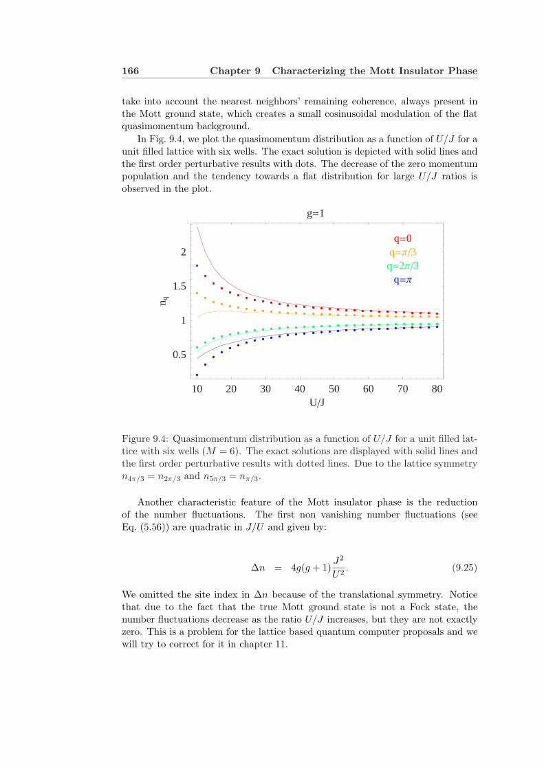
166 Chapter 9 Characterizing the Mott Insulator Phase
take into account the nearest neighbors’ remaining coherence, always present inthe Mott ground state, which creates a small cosinusoidal modulation of the flatquasimomentum background.
In Fig. 9.4, we plot the quasimomentum distribution as a function of U/J for aunit filled lattice with six wells. The exact solution is depicted with solid lines andthe first order perturbative results with dots. The decrease of the zero momentumpopulation and the tendency towards a flat distribution for large U/J ratios isobserved in the plot.
10 20 30 40 50 60 70 80UJ
0.5
1
1.5
2
n q
g=1
q=0q=Π3
q=2Π3q=Π
Figure 9.4: Quasimomentum distribution as a function of U/J for a unit filled lat-tice with six wells (M = 6). The exact solutions are displayed with solid lines andthe first order perturbative results with dotted lines. Due to the lattice symmetryn4π/3 = n2π/3 and n5π/3 = nπ/3.
Another characteristic feature of the Mott insulator phase is the reductionof the number fluctuations. The first non vanishing number fluctuations (seeEq. (5.56)) are quadratic in J/U and given by:
∆n = 4g(g + 1)J2
U2. (9.25)
We omitted the site index in ∆n because of the translational symmetry. Noticethat due to the fact that the true Mott ground state is not a Fock state, thenumber fluctuations decrease as the ratio U/J increases, but they are not exactlyzero. This is a problem for the lattice based quantum computer proposals and wewill try to correct for it in chapter 11.
9.2 Harmonic confinement plus lattice 167
We conclude this section by using the first order perturbation theory results,to crudely estimate the critical transition point. Quantum phase transitions suchas the superfluid to Mott insulator transition can be understood based on thephenomena of level crossing: as a characteristic parameter is changed (in this caseU/J), at some critical point a state that was an excited state becomes the newground state of the system. If we use this criteria to calculate the critical pointand use Eq. (9.22) we get
(U/J)c ≈ 2(2g + 1) ∼ 4g (9.26)
This result only applies for the one dimensional case. It is a factor of twosmaller than the calculated value from mean field theory (Eq. 3.9) but it is inbetter agreement with numerical Monte Carlo simulations and strong couplingexpansions which predict a critical point for a unit filled lattice of (U/J)c ≈ 4.65[78, 79].
9.2 Harmonic confinement plus lattice
In this section we consider a one dimensional optical lattice in the presence of amagnetic confinement with oscillation frequency ωT . We assume that the magnetictrap has its minimum at the lattice site n = 0. The magnetic confinement intro-duces a characteristic energy scale Ω = ma2ωT /2, so that Vn = Ωn2 (see Eq.(6.1)).We first focus on the case in which the system has an odd number of atoms.
For the analysis we are also going to consider a parameter regime where
U >Ω(N − 1)2
4, (9.27)
ΩN > J. (9.28)
The first condition expresses the requirements that the on site interaction energyU must be bigger than the trapping energy of the most externally trapped atom,so multiple atom occupation in any well is inhibited. The second states the re-quirement that the kinetic energy must be smaller than the potential energy costfor an atom at the edge of the atomic cloud to tunnel to the next unoccupied site.Thus it is energetically costly for the atoms to tunnel.
In this parameter regime the Bose-Hubbard Hamiltonian can be split into twoparts: an unperturbed part which includes the interaction and potential energyand which is diagonal in a Fock state representation, and a kinetic energy partwhich is going to be treated as a perturbation.
H = H(0) + δH, (9.29)
H(0) = Ω∑
n
n2a†n an +12U
∑n
a†na†nanan, (9.30)
δH = −J∑
n
(a†n an+1 + a†n+1 an ). (9.31)

168 Chapter 9 Characterizing the Mott Insulator Phase
With the constraints Eq. (9.27) and Eq. (9.28) we are guaranteed that to zerothorder in perturbation theory, the ground state of the system consists of a unit filledcentral core comprising N wells in the central region of the trap, surrounded byexternal empty sites, which in solid state language can be called a sea of holes. Ifthe number of atoms is odd, due to the the assumed trap symmetry, at zero orderin perturbation theory the ground state is unique and given by:
∣∣∣Φ(0)0
⟩=
∣∣∣∣∣∣0, .., 0, 1, 1, ...., 1, 1︸ ︷︷ ︸
N sites
, 0, .., 0
⟩. (9.32)
The unperturbed ground state energy is
E(0)0 =
Ω24
N(N2 − 1). (9.33)
The zeroth order low lying excitations consist of 1-ph excitations and another kindof excitations which we refer as n-hh excitations. In the following we proceed todescribe them in more detail:
• One particle hole excitation (1-ph)
The 1-ph excitations are described by the Fock states,∣∣∣Ψph
nm
⟩, with an extra
particle at site m and a hole at the site n, both inside the central core.
∣∣∣Φ(0)iph
⟩≡
∣∣∣Ψphmn
⟩(9.34)
=
∣∣∣∣∣0, .., 0, 1, ..., 2︸︷︷︸m
, ..., 0︸︷︷︸n
, .., 1, 0, .., 0
⟩.
As opposed to the translationally invariant system, the presence of the trapbreaks the degeneracy and the 1-ph excitations are not degenerate at zeroorder. Their energy is given by the interaction energy cost U to create a1-ph pair plus the potential energy cost due to the trap:
Eph(0)nm = E
(0)0 + U + Ω(m2 − n2). (9.35)
with n and m integers, n,m = −N−12 , . . . , N−1
2 .
• Hole hopping excitations (n-hh)
These excitations are described by the states with a maximum of one particleper well and holes inside the inner central core. They have to be included inthe trapped system because of the reservoir of holes surrounding the central
9.2 Harmonic confinement plus lattice 169
core which brings an extra degree of delocalization. Because the n-hh excita-tions are only due to the transfer of holes to the inner core, they don’t havethe interaction energy cost U for having two particles at the same site andtherefore they can be lower in energy than the 1-ph excitations. We label the1-hh, states with only one hole inside the central core, by
∣∣Ψhhmn
⟩. Explicitly
they are given by:
∣∣∣Φ(0)ihh
⟩≡
∣∣∣Ψhhmn
⟩(9.36)
=
∣∣∣∣∣0, .., 1︸︷︷︸n
, .., 0, 1, ..., 0︸︷︷︸m
, .., 1, 0, .., 0
⟩.
The zero order energy cost to create 1-hh excitations is:
Ehh(0)nm = E
(0)0 + Ω(m2 − n2), (9.37)
with n and m integers such that |n| > (N − 1)/2 and |m| < (N − 1)/2
At first order the kinetic energy term mixes the unperturbed ground state withthe 1-ph excitation which have the extra particle and the hole at adjacent sitesand with the 1-hh excitations were the most external trapped atom tunnels to thefirst available vacant site. The ground state wave function at first order is thengiven by
∣∣∣Φ(1)0
⟩=
∣∣∣Φ(0)0
⟩+ 2J
(N−3)/2∑
n=−(N−1)/2
∣∣∣Ψphnn+1
⟩+
∣∣∣Ψph−n−(n+1)
⟩√
2(U − Ω(1 + 2n))
+√
2J
ΩN
∣∣Ψhhnn+1
⟩+
∣∣∣Ψhh−n−(n+1)
⟩√
2. (9.38)
The first order wave functions of the excitations directly coupled to the unper-turbed ground state are
∣∣∣Φ(1)±nph
⟩=
∣∣∣Ψphnn±1
⟩−√
2J
∣∣∣Φ(0)0
⟩
(U − Ω(1± 2n)), (9.39)
∣∣∣Φ(1)±hh
⟩=
∣∣∣Ψhh±L±(L+1)
⟩− J
∣∣∣Φ(0)0
⟩
(ΩN), (9.40)
with L = (N − 1)/2.In Fig. 9.5 we plot comparisons between the analytic (blue) and exact (red)
excitation spectra. The index n labels the eigenenergies in increasing energy order.
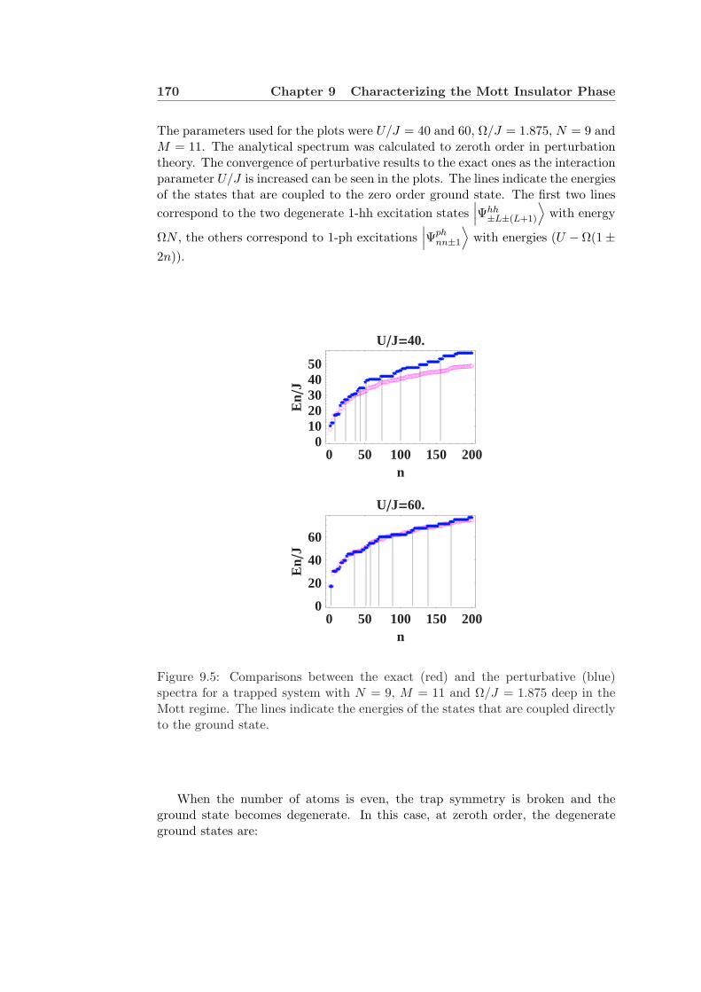
170 Chapter 9 Characterizing the Mott Insulator Phase
The parameters used for the plots were U/J = 40 and 60, Ω/J = 1.875, N = 9 andM = 11. The analytical spectrum was calculated to zeroth order in perturbationtheory. The convergence of perturbative results to the exact ones as the interactionparameter U/J is increased can be seen in the plots. The lines indicate the energiesof the states that are coupled to the zero order ground state. The first two linescorrespond to the two degenerate 1-hh excitation states
∣∣∣Ψhh±L±(L+1)
⟩with energy
ΩN , the others correspond to 1-ph excitations∣∣∣Ψph
nn±1
⟩with energies (U −Ω(1±
2n)).
0 50 100 150 200n
0
20
40
60
En
J
UJ=60.
0 50 100 150 200n
01020304050
En
J
UJ=40.
Figure 9.5: Comparisons between the exact (red) and the perturbative (blue)spectra for a trapped system with N = 9, M = 11 and Ω/J = 1.875 deep in theMott regime. The lines indicate the energies of the states that are coupled directlyto the ground state.
When the number of atoms is even, the trap symmetry is broken and theground state becomes degenerate. In this case, at zeroth order, the degenerateground states are:

9.3 Conclusions 171
∣∣∣Φ(0)0±
⟩=
1√2
(∣∣∣Φ(0)L
⟩±
∣∣∣Φ(0)R
⟩), (9.41)
∣∣∣Φ(0)L
⟩=
∣∣∣∣∣∣0, ..., 0, 1, 1, 1, ...., 1, 1︸ ︷︷ ︸
N−1 sites
, 0, .., 0
⟩,
∣∣∣Φ(0)R
⟩=
∣∣∣∣∣∣0, .., 0, 1, 1, ...., 1, 1︸ ︷︷ ︸
N−1 sites
, 1, 0, .., 0
⟩.
When the system has an even number of atoms, there are always going to be anonzero number fluctuation at the trap edge. Because the states
∣∣∣Φ(0)L
⟩and
∣∣∣Φ(0)R
⟩
are not coupled by the Bose-Hubbard Hamiltonian at first order, the previous anal-ysis we did for the system with an odd number of atoms can be straightforwardlyextended to the even case.
The constraint ΩN > J used for the analysis above can be an importantexperimental restriction if the total number of trapped atoms is large. In theregime where ΩN < J , but still U > Ω(N/2)2, the energy splitting between 1-phexcitations induced by the trap is small and degenerate perturbation theory mustbe used at first order. An analytic treatment becomes really difficult, nevertheless,it is possible to have a qualitative analysis of the system. In this case, the systemcan be divided in two parts: a central unit filled core comprising K < N wellsat the center of the trap and a superfluid layer surrounding the central core withmaximum one atom per lattice site where the mobility of the holes is high. Thesize K of the unit filled central core is determined by the strength of the magneticconfinement, K ∼ J/Ω. The properties of the unit filled core can be described toa good approximation by the commensurate homogeneous results. On the otherhand, the atoms surrounding the central core are almost free to tunnel and theyhave superfluid like properties.
9.3 Conclusions
In summary, in this chapter we have described the basic properties of the Mottinsulating phase both in translationally invariant and harmonically trapped sys-tems. All the results derived here are going to be used as the starting point forthe calculations in the following chapters.

172 Chapter 9 Characterizing the Mott Insulator Phase

Chapter 10
Bragg Spectroscopy
To date, the primary observable used to study ultra cold atoms in an optical latticehas been the momentum distribution of the system, observed after ballistic expan-sion. In particular, this type of measurement has been used to reveal the phasecoherence between sites in the lattice and has been a really useful technique tocharacterize the superfluid phase. However, the disappearance of the interferencepattern is not a conclusive diagnostic of the Mott phase. Recent analysis showsthat this is more correctly related to the degree of condensate depletion. Indeed,for this reason, the diagnostic tool used in the experiments by Greiner et al. [46],to prove the achievement of the Mott phase, was to apply a potential gradient tothe lattice and show the presence of a gap in the excitation spectrum.
Moreover, because the usual procedure for producing the Mott insulator state isto begin with a magnetically trapped Bose-Einstein condensate (with no discerniblethermal component), and slowly load it into an optical lattice, finite temperatureeffects or non-adiabatic ramping of the lattice may lead to the production of animperfect Mott phase. As more elaborate experiments are undertaken with opticallattices in the strongly correlated regime it will be crucially important to diagnosethe properties of the states produced.
The results we present here suggest that Bragg spectroscopy can not only giveinformation about the excitation spectrum, which is a crucial diagnostic of theMott insulator phase as characterized by the opening of a gap, but that it can alsobe used in the Mott regime to estimate the temperature of the system. Specifically,we study the linear response to Bragg spectroscopy of cold atoms loaded in a onedimensional optical lattice based on a perturbative analysis. We obtain analyticalexpressions for the dynamical structure factor and use them to calculate the energydeposited into the system. We also test the accuracy of our approximations bycomparing them with numerical solutions obtained by diagonalizing the Bose-Hubbard Hamiltonian for moderate number of atoms and wells. The calculationsare done for translationally invariant lattices and in the presence of an harmonicexternal potential. First we start by reviewing the basic formalism that describesBragg spectroscopy.
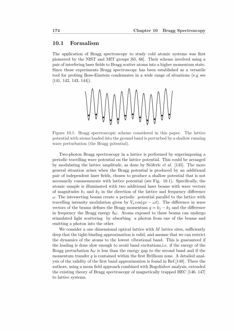
174 Chapter 10 Bragg Spectroscopy
10.1 Formalism
The application of Bragg spectroscopy to study cold atomic systems was firstpioneered by the NIST and MIT groups [65, 66]. Their scheme involved using apair of interfering laser fields to Bragg scatter atoms into a higher momentum state.Since those experiments Bragg spectroscopy has been established as a versatiletool for probing Bose-Einstein condensates in a wide range of situations (e.g see[141, 142, 143, 144]).
Figure 10.1: Bragg spectroscopic scheme considered in this paper. The latticepotential with atoms loaded into the ground band is perturbed by a shallow runningwave perturbation (the Bragg potential).
Two-photon Bragg spectroscopy in a lattice is performed by superimposing aperiodic travelling wave potential on the lattice potential. This could be arrangedby modulating the lattice amplitude, as done by Stoferle et al. [145]. The moregeneral situation arises when the Bragg potential is produced by an additionalpair of independent laser fields, chosen to produce a shallow potential that is notnecessarily commensurate with lattice potential (see Fig. 10.1). Specifically, theatomic sample is illuminated with two additional laser beams with wave vectorsof magnitudes k1 and k2 in the direction of the lattice and frequency differenceω. The intersecting beams create a periodic potential parallel to the lattice withtravelling intensity modulation given by Vo cos(qx − ωt). The difference in wavevectors of the beams defines the Bragg momentum q = k1 − k2 and the differencein frequency the Bragg energy ~ω. Atoms exposed to these beams can undergostimulated light scattering by absorbing a photon from one of the beams andemitting a photon into the other.
We consider a one dimensional optical lattice with M lattice sites, sufficientlydeep that the tight-binding approximation is valid, and assume that we can restrictthe dynamics of the atoms to the lowest vibrational band. This is guaranteed ifthe loading is done slow enough to avoid band excitations,i.e. if the energy of theBragg perturbation ~ω is less than the energy gap to the second band and if themomentum transfer q is contained within the first Brillioun zone. A detailed anal-ysis of the validity of the first band approximation is found in Ref.[148]. There theauthors, using a mean field approach combined with Bogoliubov analysis, extendedthe existing theory of Bragg spectroscopy of magnetically trapped BEC [146, 147]to lattice systems.

10.1 Formalism 175
As shown in chapter 3, under the single-band approximation the system is de-scribed by the Bose-Hubbard Hamiltonian, which we will denote as Ho. Hereafterwe assume, unless otherwise specified, a harmonic magnetic confinement such thatVn = Ωn2. In the tight-binding approximation, the Hamiltonian describing theBragg perturbation is given by
HB =12Vo(ρ†qe
−iωt + ρqeiωt). (10.1)
The density fluctuation operator ρ†q is defined as
ρ†q =M−1∑
m,n=0
In,mq a†man, (10.2)
withIn,mq =
∫dxeiqxw∗0(x− am)w0(x− an), (10.3)
where w0(x) is the Wannier orbital centered at the origin of the lowest vibra-tional band. To calculate In,m
q we approximate the Wannier orbitals by Gaus-sians localized at the bottom of the potential wells , φ0(x − an) ∼ exp[−(x −an)2/2a2
ho]/(π1/4√aho), where the width aho can be estimated by minimizing theground state energy. For a lattice potential of the form ERVlat sin2(πx/a), withER the recoil energy of the atoms, aho scales like aho ∼ (Vlat)−1/4a/π. Ne-glecting the overlap between Wannier orbitals located in different sites we getIn,mq ∼ Iqδn,m exp(ia(n + m)q/2), where δn,m is the Kronecker delta function.
Then
Iq = exp(− 1√
Vlat
( qa
2π
)2)
. (10.4)
Notice that Iq approaches one for small qa and deep lattices. Using the approxi-mate expression for In,m
q we can rewrite the density operator as:
ρ†q = Iq
M−1∑
m=0
a†mameiqma. (10.5)
To simplify the notation and to have a better physical understanding of theexcitations induced by the Bragg perturbation, it is convenient to introduce thequasimomentum field operator bk which annihilates an atom with quasimomentumk, and is defined as the Fourier transform of the field operator an, i.e., bk =
1√M
∑Mn=1 eiknaan. The quasimomentum k can assume only discrete values which
are integer multiples of 2πMa .
In the quasimomentum basis the operator ρ†q can be written as
ρ†q = Iq
M−1∑
k=0
b†k+q bk, (10.6)

176 Chapter 10 Bragg Spectroscopy
where we have assumed that q can be also expressed as an integer multiple of2πMa . By writing the Bragg perturbation potential in the quasimomentum basis itcan be seen that the two means by which momentum is imparted to the atomicsample,is either by promoting an atom from quasimomentum k to k + q or bydemoting a particle with momentum k to k − q.
10.2 Observables
Useful experimental observables in Bragg spectroscopy are related to the density-density response function. Here we focus our attention on the imparted momentumand energy, which can be measured by time-of-flight techniques. In this sectionwe elaborate on the form of these observables.
In the tight-binding approximations the total momentum is given by
P =∑
k
~kb†k bk. (10.7)
From the Heisenberg equations of motion we get
dP
dt=
i
~
[H,P
]=
i
~
([HB,P
]+
[Ho,P
])(10.8)
= − iqVo
2(ρ†qe
−iωt − ρqeiωt)− 2ΩX. (10.9)
where H is the total Hamiltonian, H = Ho + HB, and X is the center of massposition given by X =
∑n(na)a†nan. The second term in the momentum rate
equation is just related to the force felt by atoms due to the presence of an harmonicexternal confinement. On the other hand, the first term takes into account the rateof change of the momentum due to the Bragg perturbation. If the perturbation isapplied for a time short compared to the oscillator period tosc= 2π√
4JΩathe second
term in the right-hand-side is small and can be neglected in the calculations.The energy change rate is
dHo
dt=
i
~
[HB,Ho
]=
i
~
[HB,H
], (10.10)
= −12Vo
(e−iωt dρ†q
dt+ eiωt dρq
dt
).
Because the energy of a closed system is conserved, as opposed to the momentumrate equation, the energy change rate is independent of the magnetic potential andonly depends on the applied Bragg perturbation.
10.3 Linear response 177
10.3 Linear response
The first order variation δ〈 ˆO(t)〉 of the thermal average of an observable ˆO(t) withrespect to its mean value due to a weak perturbation HB applied to a system att = to , is given by the Kubo formula [51]
δ⟨O(t)
⟩=
i
~
∫ t
to
dτ⟨[
HB(τ), O(t)]⟩
, (10.11)
where the operators O(t) and HB(τ) are in the Heisenberg representation withrespect to the time independent hamiltonian Ho, and the expectation value istaken using the equilibrium state of the system.
For the particular case where the observables are the momentum and energyrates, we get after some algebra :
δ
⟨dP
dt
⟩= ~q
(Vo
2~
)2
× (10.12)
∫ t
to
dτ(e−iω(τ−t)
⟨[ρ†q(τ), ρq(t)
]⟩− eiω(τ−t)
⟨[ρq(τ), ρ†q(t)
]⟩
+e−iω(τ+t)⟨[
ρ†q(τ), ρ†q(t)]⟩− eiω(τ+t) 〈[ρq(τ), ρq(t)]〉
)− 2Ωδ
⟨X
⟩,
δ
⟨dH
dt
⟩= − i
~
(Vo
2
)2
× (10.13)
∫ t
to
dτ
(e−iω(τ−t) d
dt
⟨[ρ†q(τ), ρq(t)
]⟩− eiω(τ−t) d
dt
⟨[ρq(τ), ρ†q(t)
]⟩
+e−iω(τ+t) d
dt
⟨[ρ†q(τ), ρ†q(t)
]⟩− eiω(τ+t) d
dt〈[ρq(τ), ρq(t)]〉
).
We now introduce the functions S(q, ω) and R(q, ω) given by
⟨ρ†q(τ)ρq(t)
⟩=
∫e−iω(τ−t)S(q, ω)dω, (10.14)
⟨ρ†q(τ)ρ†q(t)
⟩=
∫eiω(τ+t)R(q, ω)dω. (10.15)
In terms of these functions it can be seen that since⟨[
ρ†q(τ), ρ†q(t)]⟩
=⟨[
ρq(τ), ρq(t)]⟩
=0 Eq. (10.13) and Eq. (10.14) reduce to:
δ
⟨dP
dt
⟩= 2~q
(Vo
2~
)2 ∫dω′
(S(q, ω′)− S(−q,−ω′)
)×(
sin ((ω − ω′)t)(ω − ω′)
)− 2Ωδ
⟨X
⟩,

178 Chapter 10 Bragg Spectroscopy
δ
⟨dH
dt
⟩=
2~
(Vo
2
)2 ∫dω′ω′
(S(q, ω′)− S(−q,−ω′)
)× (10.16)
(sin ((ω − ω′)t)
(ω − ω′)
).
where we have set to = 0. The quantity S(q, ω), the Fourier transform of densitycorrelations, is the so called dynamic structure factor and is given by
S(q, ω) =1Z
∑
ij
e−βEi |〈i| ρq |j〉|2 δ(ω − ωij) (10.17)
≡∑
ij
Sij(q)δ(ω − ωij). (10.18)
where |i〉 and Ei are eigenstates and eigenenergies of the unperturbed Hamiltonian,e−βEi is the usual Boltzmann factor with β = 1/kBT where kB is Boltzmann’sconstant and T the temperature, Z is the canonical partition function, ~ωij =Ej −Ei and Sij(q) ≡ 1
Z e−βEi |〈i| ρq |j〉|2 .
Notice that because atoms could be scattered by absorbing a photon fromeither one of the laser beams the response of the system is determined not onlyby S(q, ω) but by the combination S(q, ω′) − S(−q,−ω′). If the perturbationis applied for a time long with respect to the frequency of the applied field themomentum and energy rates approach the golden rule results.
Performing the frequency integration we get
δ
⟨dP
dt
⟩= 2~q
(Vo
2~
)2 ∑
ij
(Sij(q)
(sin ((ω − ωij)t)
ω − ωij
)(10.19)
−Sij(−q)(
sin ((ω + ωij)t)ω + ωij
))− 2Ωδ
⟨X(t)
⟩,
δ
⟨dH
dt
⟩= 2
(Vo
2~
)2 ∑
ij
~ωij
(Sij(q)
(sin ((ω − ωij)t)
ω − ωij
)(10.20)
+Sij(−q)(
sin ((ω + ωij)t)ω + ωij
)).
The total momentum and energy transfer after applying the Bragg perturbationcan be obtained by integrating the above equations. We get as a final result that

10.4 Zero-temperature regime 179
δ⟨P
⟩= ~q
(Vo
~
)2 ∑
ij
(Sij(q)
(sin ((ω − ωij)τ/2)
ω − ωij
)2
(10.21)
−Sij(−q)(
sin ((ω + ωij)τ/2)ω + ωij
)2)− 2Ω/a
∫ τ
0δ⟨X(t)
⟩dt
δ⟨H
⟩=
(Vo
~
)2 ∑
ij
~ωij
(Sij(q)
(sin ((ω − ωij)τ/2)
ω − ωij
)2
(10.22)
+Sij(−q)(
sin ((ω + ωij)τ/2)ω + ωij
)2)
,
where τ is the duration of the perturbation.
10.4 Zero-temperature regime
10.4.1 Bogoliubov approach
In this section we use the zero temperature Bogoliubov approximation for atoms inan optical lattice to study the dynamical structure factor in the superfluid regime.Because quadratic approximations were discussed in detail in in chapter 5, we referthe reader to this chapter for details.
Under the Bogoliubov approximation the field operator at lattice site n iswritten as a complex number zn plus small fluctuations δ =
∑Ms6=0(us
nαs −v∗sn α†s ),with us
n, vsn the quasiparticle amplitudes. Using this ansatz in Eq.(10.17) we get
an expression for the dynamical structure factor given by
ST=0(q, ω) = S0(q)δ(ω) +∑
i
Si(q)δ(ω − ωBi ), (10.23)
S0(q) ≡∣∣∣∣∣
M∑
n=1
|zn|2eiqan
∣∣∣∣∣
2
, (10.24)
Si(q) ≡∣∣∣∣∣∑
n
(znu∗in − z∗nv∗in )eiqan
∣∣∣∣∣2
. (10.25)
Translationally invariant system
To understand many-body effects included in the Bogoliubov approximation westart by studying the case of a translationally invariant lattice (Vn = 0) withN atoms, M wells and periodic boundary conditions. Using the results for thequasiparticle amplitudes and energies calculated using the improved Popov ap-proximation, which was shown to be the best quadratic approximation we get:
180 Chapter 10 Bragg Spectroscopy
S(q, ω) = N2δ(ω) + Mnoεq
ωBq
δ(ω − ωBq /~) (10.26)
= N2δ(ω) + MnoS(q)δ(ω − ωBq /~), (10.27)
with no given by Eq. (5.136), εk = 4J sin2(ak/2) and ωBk =
√ε2k + 2nUεk. Here n
is the total density n = N/M . Notice that due to the translational invariance ofthe system, the quasimomentum is a good quantum number and only quasiparticlestates that have the same quasimomentum as the transferred momentum q areexcited.
For small q, the structure factor behaves like√
J2Unq which is just the free
particle expression with the bare particle mass m replaced by the effective mass,m∗ = ~2/2Ja2 (a the lattice spacing). Suppression of S(q) in the phonon regime isa direct consequence of the importance of quantum correlations in the long wave-length limit. On the other hand, away from the phonon regime, the presence ofthe optical lattice changes the behavior of S(q) in a drastic way. As opposed tothe free case where at high transferred momenta ωB
q ∼ q2 and S(q) approachesone, the periodic potential modifies the single particle dispersion relation, whichbecomes always bounded by 4J . The term proportional to 2nUεk dominates evenat high momenta and many-body effects play a crucial role.
In Fig.10.2 we show the energy δ〈H〉 imparted to the system as a function ofthe frequency ω of the Bragg probe, for different values of and U/J and of themomentum q. The blue curve corresponds to the solution using the Bogoliubovapproximation and the red one to the solution obtained by the exact diagonal-ization of the Bose-Hubbard Hamiltonian. The number of lattice sites and wellsused in the plots were M = N = 9. For U/J = 0.001 the Bogoliubov and exactcurves perfectly overlap. The agreement is expected as the non-interacting Hamil-tonian is quadratic and therefore exactly matches the Bogoliubov Hamiltonian.The almost non interacting regime may be experimentally achieved by varyingthe onsite interaction energy U independently of J , by means of a Feshbach res-onance that changes the scattering length [20, 21]. For U/J = 1 the agreementis good only for the low momentum q = 2π/9. The agreement for low momentacan be understood by the fact that for low q the Bragg spectroscopy is probingthe long wave-length modes. These modes have a phonon-like dispersion relationand are almost not affected by the presence of the lattice. In general Bogoliubovquasi-particle states correspond to solutions of the approximate Hamiltonian witha plane-wave character which are only valid in the weakly interacting regime. Asquantum correlations become important, the exact eigenstates of the interactingsystem do not necessarily have the simple plane wave character,(see Ref. Lieband Liniger [149]), especially in the commensurate filling situation where for acritical value of U/J the system exhibits the superfluid-Mott insulator transition.However the unit filled commensurate case is the worse scenario, and as discussedin chapter 5, for non commensurate fillings or commensurate systems with larger

10.4 Zero-temperature regime 181
filling factor we expect the validity of the Bogoliubov approximation to extendover a larger range of U/J values.
As a final remark, it is important to point out that the small oscillations inFig. 10.2 are due to the square shape of the applied Bragg pulse. These oscillationswould disappear if instead a pulse with Gaussian profile is applied.
0 2 4 6 8 10 12ΩJ
020406080
∆EHV
o2 JL
UJ=2. q=2Π9
0 2 4 6 8 10 12ΩJ
0
200
400
600
∆EHV
o2 JL
UJ=2. q=8Π9
0 2 4 6 8ΩJ
020406080
100
∆EHV
o2 JL
UJ=1. q=2Π9
0 2 4 6 8ΩJ
0
200
400
600
800
∆EHV
o2 JL
UJ=1. q=8Π9
0 1 2 3 4 5 6ΩJ
020406080
100
∆EHV
o2 JL
UJ=0.001 q=2Π9
0 1 2 3 4 5 6ΩJ
0200400600800
∆EHV
o2 JL
UJ=0.001 q=8Π9
Figure 10.2: Imparted energy: Comparisons between the the exact and Bogoliubovapproximation for N = M = 9. The horizontal axis is in units of ~. For the plotwe used Jτ/~ = 10. See text Eq. (10.23).
10.4.2 Inhomogeneous system
Using the quasiparticle amplitudes derived under the T.F. approximation (seesection 5.6.2), we get an expression for the dynamical structure factor given by
S(q, ω) = 9N2
(sin(x)− x cos(x)
x3
)2
δ(ω)
+~ω∗
8U
∑
i
(i(i + 1)(2i + 1))|Pi(x)|2δ(ω − ω∗√
i(i + 1)/2)(10.28)
where x ≡ qaRTF and Pn(x) =∫ 1−1 Pn(u)eiuxdu.
An alternative way to calculate the dynamical structure factor is to use the socalled local density approximation (LDA). This approximation is valid for largecondensates, where the density profile varies in a smooth way and the systembehaves locally as an uniform gas. Using a LDA the dynamical structure factorcan be written as
182 Chapter 10 Bragg Spectroscopy
SLDA(q, ω) =
(∑m
z(m)eiqam
)δ(ω) + εs
∑m
|z(m)|2~ωB
q (m)δ(~ω − ωB
q (m)). (10.29)
Here ωBq (m) is the local homogeneous Bogoliubov dispersion relation with n re-
placed by the local density in the trap. The LDA ignores the Doppler effectassociated with the spreading of the momentum distribution of the condensateand therefore it is not valid for large momentum transfers.
To test the validity of the HFB-Popov approximation to describe the energyimparted to the system by Bragg spectroscopy in the trapped case we use a systemwith 11 lattice sites and 9 atoms. Unfortunately for such a small number of atomsand wells the assumptions under which the analytic Thomas Fermi expressionswere developed, i.e. large number of atoms and smooth variations of the densityprofile, do not apply. Therefore for the case with M = 11, N = 9 we restrictourselves to comparisons between numerical solutions of the HFB-Popov equationsand solutions found by the exact diagonalization of the many-body Hamiltonian.We solve numerically Eqs.(5.113) -(5.117) to obtain the quasi-particle energy andamplitudes. We then use them to calculate the imparted energy. In the presence ofthe trap, the number of occupied wells for a fixed number of atoms depends on thetrap frequency, particles are not necessarily uniformly distributed throughout thelattice, and therefore commensurability is only meaningful locally. This explainswhy in contrast to the commensurate homogeneous system, the agreement betweenthe two solutions is good up to U/J = 5 for the chosen parameters, as shown inFig. 10.3. The failure of the HFB-Popov approximation for U/J ∼ 10 can also beobserved in the density plots, as shown in Fig. 10.4.
The multiple peaks depicted in the plots are due to the external trapping po-tential, which not only discretizes the spectrum but also changes the plane wavecharacter of the quasiparticle amplitudes. Therefore, for a given transfer momen-tum q different quasiparticle modes can be excited. In Fig.10.3, we explicitly showwith a line the position of the quasiparticle energies.Similar to the homogeneouscase, the lower the transfer momentum q, the better is the agreement between theHFB-Popov results and the exact solution.
For small systems such as the one in consideration discretization effects cannot be ignored. On the other hand, if the inverse of the transfer momentum isbigger than the size of the condensate wave function, then to first approximationthe discretization in the excitation spectrum can be safely ignored and the systemcan be treated as locally uniform. Instead of distinguishable peaks the responsecurve becomes smooth.
To explore the validity of Eq.(10.28) derived under the Thomas-Fermi approx-imation we plot in Fig. 10.5 S(q, ω) vs. ω for different transfer momenta. Theparameters used for the plot were U/J = 0.2, Ω/J = 9.5×10⁻⁴ and N = 100. Forthese parameters we believe the HFB-Popov should give a good description of thesystem. In chapter 5 we showed that in the regime when the TF approximation isvalid, it gives a very good description of the low lying excitations. However it fails
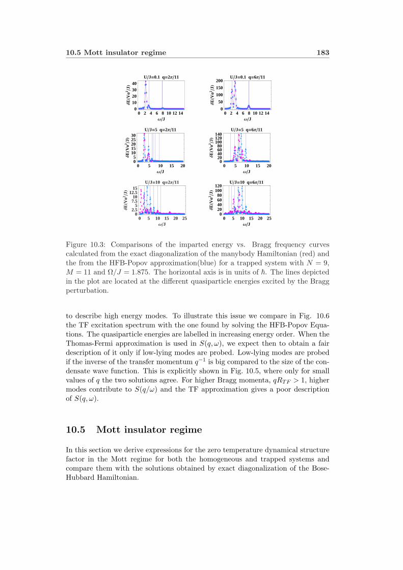
10.5 Mott insulator regime 183
0 5 10 15 20 25ΩJ
02.5
57.510
12.515
∆EHV
o2 JL
UJ=10 q=2Π11
0 5 10 15 20 25ΩJ
020406080
100120
∆EHV
o2 JL
UJ=10 q=6Π11
0 5 10 15 20ΩJ
05
1015202530
∆EHV
o2 JL
UJ=5 q=2Π11
0 5 10 15 20ΩJ
020406080
100120140
∆EHV
o2 JL
UJ=5 q=6Π11
0 2 4 6 8 10 12 14ΩJ
010203040
∆EHV
o2 JL
UJ=0.1 q=2Π11
0 2 4 6 8 10 12 14ΩJ
0
50
100
150
200
∆EHV
o2 JL
UJ=0.1 q=6Π11
Figure 10.3: Comparisons of the imparted energy vs. Bragg frequency curvescalculated from the exact diagonalization of the manybody Hamiltonian (red) andthe from the HFB-Popov approximation(blue) for a trapped system with N = 9,M = 11 and Ω/J = 1.875. The horizontal axis is in units of ~. The lines depictedin the plot are located at the different quasiparticle energies excited by the Braggperturbation.
to describe high energy modes. To illustrate this issue we compare in Fig. 10.6the TF excitation spectrum with the one found by solving the HFB-Popov Equa-tions. The quasiparticle energies are labelled in increasing energy order. When theThomas-Fermi approximation is used in S(q, ω), we expect then to obtain a fairdescription of it only if low-lying modes are probed. Low-lying modes are probedif the inverse of the transfer momentum q−1 is big compared to the size of the con-densate wave function. This is explicitly shown in Fig. 10.5, where only for smallvalues of q the two solutions agree. For higher Bragg momenta, qRTF > 1, highermodes contribute to S(q/ω) and the TF approximation gives a poor descriptionof S(q, ω).
10.5 Mott insulator regime
In this section we derive expressions for the zero temperature dynamical structurefactor in the Mott regime for both the homogeneous and trapped systems andcompare them with the solutions obtained by exact diagonalization of the Bose-Hubbard Hamiltonian.
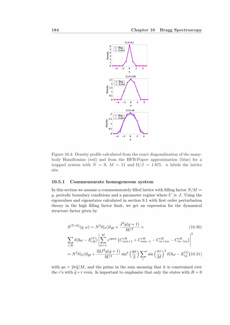
184 Chapter 10 Bragg Spectroscopy
-4 -2 0 2 4n
0123456
Den
sity
UJ=0.1
ExactBog.
-4 -2 0 2 4n
0
0.5
1
1.5
2
2.5
Den
sity
UJ=5.05
ExactBog.
-4 -2 0 2 4n
0
0.5
1
1.5
2
Den
sity
UJ=10.
ExactBog.
Figure 10.4: Density profile calculated from the exact diagonalization of the many-body Hamiltonian (red) and from the HFB-Popov approximation (blue) for atrapped system with N = 9, M = 11 and Ω/J = 1.875. n labels the latticesite.
10.5.1 Commensurate homogeneous system
In this section we assume a commensurately filled lattice with filling factor N/M =g, periodic boundary conditions and a parameter regime where U À J . Using theeigenvalues and eigenstates calculated in section 9.1 with first order perturbationtheory in the high filling factor limit, we get an expression for the dynamicalstructure factor given by
S(T=0)(q, ω) = N2δ(ω)δq0 +J2g(g + 1)~U2
× (10.30)
∑
r,R
δ(~ω − E(1)rR )
∣∣∣∣∣M∑
m=1
eiqam(CrR
mm+1 + CrRmm−1 − CrR
m+1m − CrRm−1m
)∣∣∣∣∣
2
= N2δ(ω)δq0 +32J2g(g + 1)
~U2sin2
(qa
2
)∑r
′sin
(πr
M
)2δ(~ω − E
(1)rq )(10.31)
with qa = 2πq/M , and the prime in the sum meaning that it is constrained overthe r’s with q + r even. Is important to emphasize that only the states with R = 0

10.5 Mott insulator regime 185
0.2 0.4 0.6 0.8ΩJ
02.5
57.510
12.515
SHq,ΩL
q= 0.17 Π
0.2 0.4 0.6 0.8ΩJ
05
101520
SHq,ΩL
q= 0.24 Π
0.2 0.4 0.6 0.8ΩJ
012345
SHq,ΩL
q= 0.034 Π
0.2 0.4 0.6 0.8ΩJ
02468
101214
SHq,ΩL
q= 0.1 Π
Figure 10.5: Dynamical structure factor vs. ~ω/J in the Thomas-Fermi (blue)and HFB-Popov (red) approximations. The horizontal axis is in units of ~. Thesystem parameters are U/J = 0.2, Ω/J = 9.5× 10⁻⁴ and N = 100.
have a dispersion relation which agrees to first order in J to the mean-field solutionfound in Ref. [151]. However, these states give zero contribution to the sum of Eq.(10.31).
In Fig. 10.7 we compare the imparted energy as a function of the Bragg fre-quency calculated using the expression of the dynamical structure factor Eq. (10.31)to results obtained by the exact diagonalization of the Bose-Hubbard Hamiltonianwith parameters N = M = 9 and U/J = 45. We show the response for two dif-ferent Bragg momenta q = 2π/9 and 8π/9. In contrast to the superfluid regime,where Bragg spectroscopy excites only the quasiparticle state with quasimomen-tum q, in the Mott regime we observe M − 1 peaks centered around U . Thedifferent peaks are due to the two dimensional character of the 1-ph dispersionrelation. The Bragg momentum q fixes one quantum number R but the other cantake M − 1 different values. In the analytic solution due to the constraint in Eq.(10.31), q + r even, only (M − 1)/2 of the possible M − 1 peaks are present. Theconstraint is a consequence of the extra symmetry introduced in the high filling fac-tor solution where similar ”effective masses” are assumed. Nevertheless, Fig. 10.7shows that even in the situation with g = 1, the peaks captured by the analyticsolution are the most relevant ones. As g is increased, as long as the perturbationanalysis is valid, we expect even better agreement. The interval of frequenciesover which the system responds has an approximate width of 4J(2g+1) cos(qa/2).The cos(qa/2) dependence indicates that as q approaches π the response width isminimized. This behavior can be observed in Fig. 10.7, when we plot the response
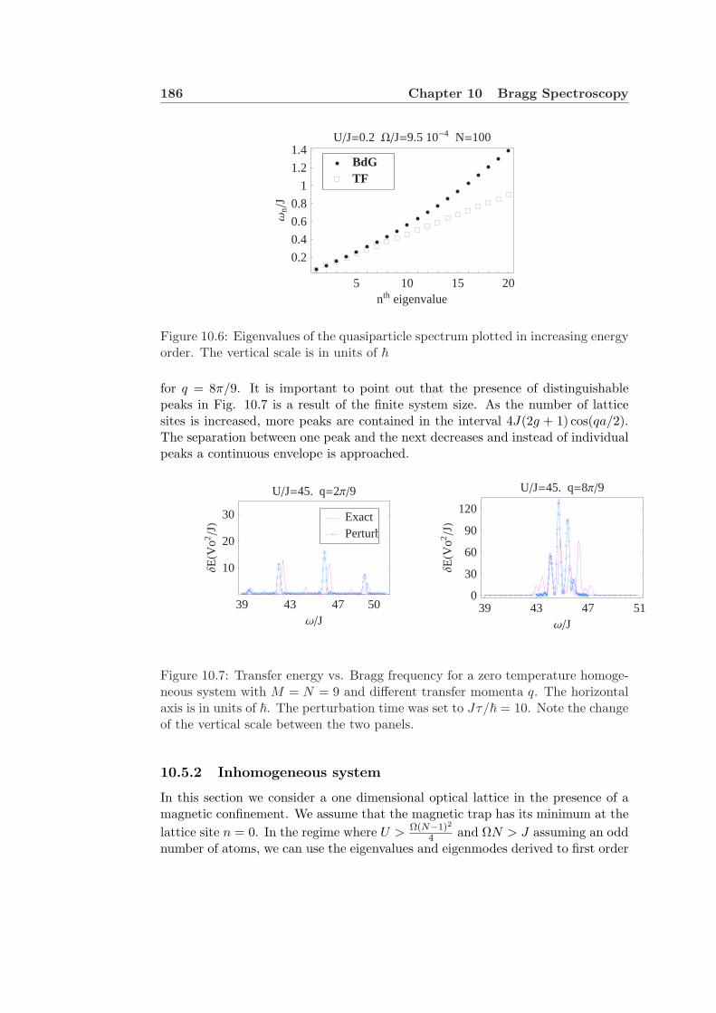
186 Chapter 10 Bragg Spectroscopy
5 10 15 20nth eigenvalue
0.2
0.4
0.6
0.8
1
1.2
1.4
Ωn
J
UJ=0.2 WJ=9.5 10-4 N=100
TFBdG
Figure 10.6: Eigenvalues of the quasiparticle spectrum plotted in increasing energyorder. The vertical scale is in units of ~
for q = 8π/9. It is important to point out that the presence of distinguishablepeaks in Fig. 10.7 is a result of the finite system size. As the number of latticesites is increased, more peaks are contained in the interval 4J(2g + 1) cos(qa/2).The separation between one peak and the next decreases and instead of individualpeaks a continuous envelope is approached.
39 43 47 50ΩJ
10
20
30
∆EHV
o2JL
UJ=45. q=2Π9
Perturb.Exact
39 43 47 51ΩJ
0
30
60
90
120
∆EHV
o2JL
UJ=45. q=8Π9
Figure 10.7: Transfer energy vs. Bragg frequency for a zero temperature homoge-neous system with M = N = 9 and different transfer momenta q. The horizontalaxis is in units of ~. The perturbation time was set to Jτ/~ = 10. Note the changeof the vertical scale between the two panels.
10.5.2 Inhomogeneous system
In this section we consider a one dimensional optical lattice in the presence of amagnetic confinement. We assume that the magnetic trap has its minimum at thelattice site n = 0. In the regime where U > Ω(N−1)2
4 and ΩN > J assuming an oddnumber of atoms, we can use the eigenvalues and eigenmodes derived to first order
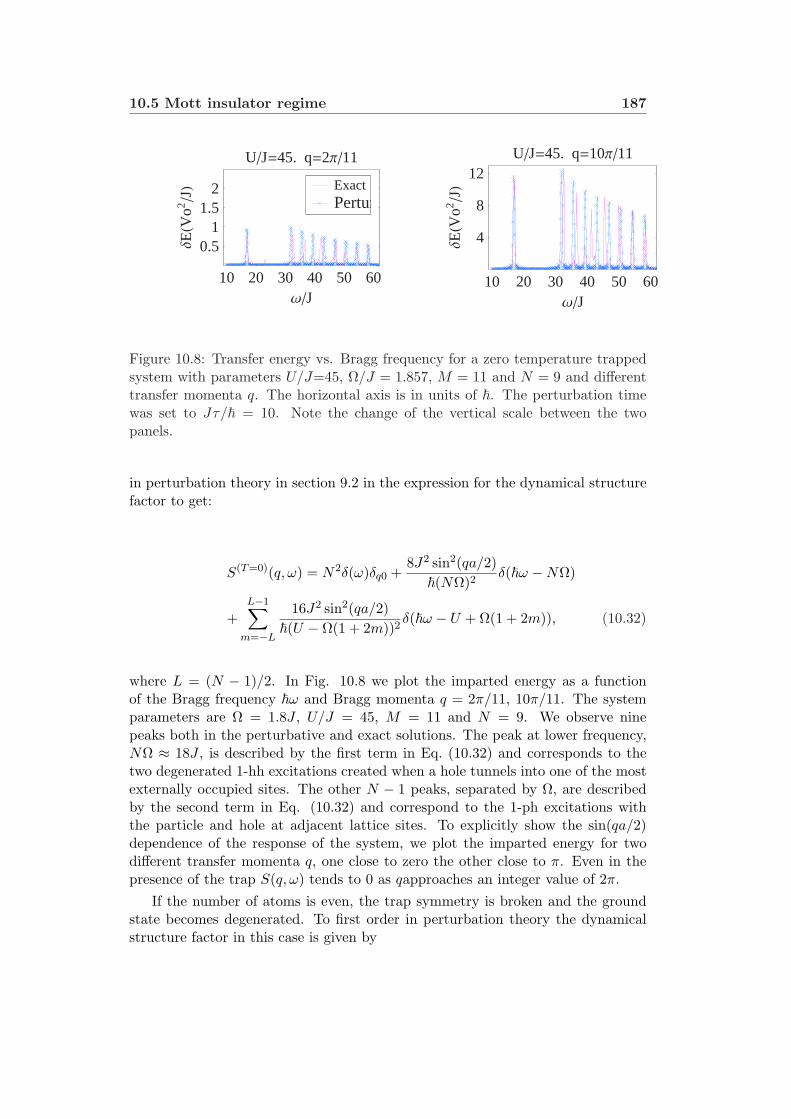
10.5 Mott insulator regime 187
10 20 30 40 50 60ΩJ
0.51
1.52
∆EHV
o2JL
UJ=45. q=2Π11
PerturbExact
10 20 30 40 50 60ΩJ
4
8
12
∆EHV
o2JL
UJ=45. q=10Π11
Figure 10.8: Transfer energy vs. Bragg frequency for a zero temperature trappedsystem with parameters U/J=45, Ω/J = 1.857, M = 11 and N = 9 and differenttransfer momenta q. The horizontal axis is in units of ~. The perturbation timewas set to Jτ/~ = 10. Note the change of the vertical scale between the twopanels.
in perturbation theory in section 9.2 in the expression for the dynamical structurefactor to get:
S(T=0)(q, ω) = N2δ(ω)δq0 +8J2 sin2(qa/2)~(NΩ)2
δ(~ω −NΩ)
+L−1∑
m=−L
16J2 sin2(qa/2)~(U − Ω(1 + 2m))2
δ(~ω − U + Ω(1 + 2m)), (10.32)
where L = (N − 1)/2. In Fig. 10.8 we plot the imparted energy as a functionof the Bragg frequency ~ω and Bragg momenta q = 2π/11, 10π/11. The systemparameters are Ω = 1.8J , U/J = 45, M = 11 and N = 9. We observe ninepeaks both in the perturbative and exact solutions. The peak at lower frequency,NΩ ≈ 18J , is described by the first term in Eq. (10.32) and corresponds to thetwo degenerated 1-hh excitations created when a hole tunnels into one of the mostexternally occupied sites. The other N − 1 peaks, separated by Ω, are describedby the second term in Eq. (10.32) and correspond to the 1-ph excitations withthe particle and hole at adjacent lattice sites. To explicitly show the sin(qa/2)dependence of the response of the system, we plot the imparted energy for twodifferent transfer momenta q, one close to zero the other close to π. Even in thepresence of the trap S(q, ω) tends to 0 as qapproaches an integer value of 2π.
If the number of atoms is even, the trap symmetry is broken and the groundstate becomes degenerated. To first order in perturbation theory the dynamicalstructure factor in this case is given by
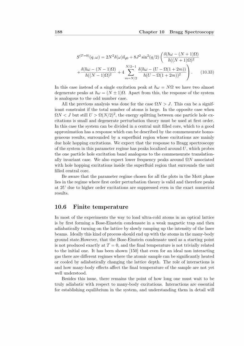
188 Chapter 10 Bragg Spectroscopy
S(T=0)(q, ω) = 2N2δ(ω)δq0 + 8J2 sin2(q/2)(
δ(~ω − (N + 1)Ω)~((N + 1)Ω)2
+δ(~ω − (N − 1)Ω)~((N − 1)Ω)2
+ 4N/2−1∑
m=N/2
δ(~ω − (U − Ω(1 + 2m))~(U − Ω(1 + 2m))2
. (10.33)
In this case instead of a single excitation peak at ~ω = NΩ we have two almostdegenerate peaks at ~ω = (N ± 1)Ω. Apart from this, the response of the systemis analogous to the odd number case.
All the previous analysis was done for the case ΩN > J . This can be a signif-icant constraint if the total number of atoms is large. In the opposite case whenΩN < J but still U > Ω(N/2)2, the energy splitting between one particle hole ex-citations is small and degenerate perturbation theory must be used at first order.In this case the system can be divided in a central unit filled core, which to a goodapproximation has a response which can be described by the commensurate homo-geneous results, surrounded by a superfluid region whose excitations are mainlydue hole hopping excitations. We expect that the response to Bragg spectroscopyof the system in this parameter regime has peaks localized around U , which probesthe one particle hole excitation band analogous to the commensurate translation-ally invariant case. We also expect lower frequency peaks around ΩN associatedwith hole hopping excitations inside the superfluid region that surrounds the unitfilled central core.
Be aware that the parameter regime chosen for all the plots in the Mott phaselies in the regime where first order perturbation theory is valid and therefore peaksat 2U due to higher order excitations are suppressed even in the exact numericalresults.
10.6 Finite temperature
In most of the experiments the way to load ultra-cold atoms in an optical latticeis by first forming a Bose-Einstein condensate in a weak magnetic trap and thenadiabatically turning on the lattice by slowly ramping up the intensity of the laserbeams. Ideally this kind of process should end up with the atoms in the many-bodyground state.However, that the Bose-Einstein condensate used as a starting pointis not produced exactly at T = 0, and the final temperature is not trivially relatedto the initial one. It has been shown [150] that even for an ideal non interactinggas there are different regimes where the atomic sample can be significantly heatedor cooled by adiabatically changing the lattice depth. The role of interactions isand how many-body effects affect the final temperature of the sample are not yetwell understood.
Besides this issue, there remains the point of how long one must wait to betruly adiabatic with respect to many-body excitations. Interactions are essentialfor establishing equilibrium in the system, and understanding them in detail will

10.6 Finite temperature 189
be really important to determine the time scales for adiabatic loading. For a deeplattice the tunneling rate seems to be the most restrictive time scale for maintainingadiabaticity. If adiabaticity were determined by the tunneling time ~/J , it wouldbe very hard to be satisfied experimentally because J decreases exponentially withthe lattice depth.
Because of these issues, it would be very interesting from an experimentalpoint of view to have a mechanism for determining the temperature of the system.What we show in this section is that Bragg spectroscopy could give informationabout the temperature, at least deep in the Mott regime. As we did for the zerotemperature case, we start by describing the superfluid case, then the deep Mottinsulator case, and finally showing numerical calculations in the regime where theMott transition takes place.
• Superfluid Regime
At finite temperature both quantum and thermal fluctuations contribute tothe depletion of the condensate. We expect the Bogoliubov approach to be agood description of the many-body system for moderate lattice depths andsmall thermal depletion. At finite temperature the occupation number of aquasiparticle state is determined by Bose statistics, ns =
⟨α†sαs
⟩with ns
the Bose distribution function ns = 1
eβωBs −1
. Taking into account thermaldepletion, the expression for the dynamical structure factor is
S(q, ω) = S0(q)δ(ω) +∑
i
(ni + 1)Si(q)δ(ω − ωBi )
+∑
i
niSi(−q)δ(ω + ωBi ) (10.34)
with S0(q) and Si(q) defined in Eqs. (10.24) and (10.25).
Even though the finite temperature dynamic structure factor is in fact dif-ferent from the zero temperature one, observables such as the imparted mo-mentum and imparted energy do not depend on S(q, ω) but on S(q, ω) −S(−q,−ω). This difference is independent of the temperature, at least at theorder of approximation at which Eq.(10.34) was calculated [15, 147, 148].
Therefore, Bogoliubov analysis shows that, provided the temperature is suf-ficient low and the interactions are weak enough that Eq.(10.34) is valid,Bragg spectroscopy is not a good method for determining the temperatureof the gas.
• Mott Regime
In the homogeneous Mott phase all the 1-ph excitations have an energy sep-aration of order U from the ground state but splitting between them of orderJ . If the temperature of the system is kBT & U/5, 1-ph excitations begin to
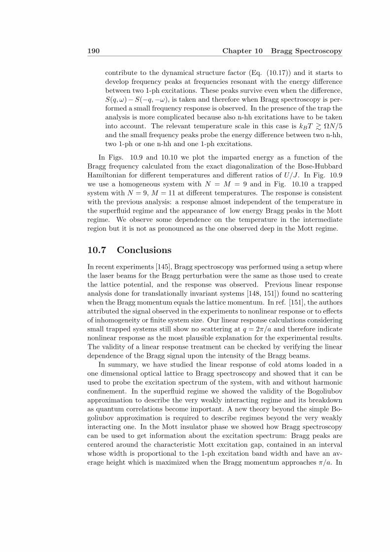
190 Chapter 10 Bragg Spectroscopy
contribute to the dynamical structure factor (Eq. (10.17)) and it starts todevelop frequency peaks at frequencies resonant with the energy differencebetween two 1-ph excitations. These peaks survive even when the difference,S(q, ω)−S(−q,−ω), is taken and therefore when Bragg spectroscopy is per-formed a small frequency response is observed. In the presence of the trap theanalysis is more complicated because also n-hh excitations have to be takeninto account. The relevant temperature scale in this case is kBT & ΩN/5and the small frequency peaks probe the energy difference between two n-hh,two 1-ph or one n-hh and one 1-ph excitations.
In Figs. 10.9 and 10.10 we plot the imparted energy as a function of theBragg frequency calculated from the exact diagonalization of the Bose-HubbardHamiltonian for different temperatures and different ratios of U/J . In Fig. 10.9we use a homogeneous system with N = M = 9 and in Fig. 10.10 a trappedsystem with N = 9, M = 11 at different temperatures. The response is consistentwith the previous analysis: a response almost independent of the temperature inthe superfluid regime and the appearance of low energy Bragg peaks in the Mottregime. We observe some dependence on the temperature in the intermediateregion but it is not as pronounced as the one observed deep in the Mott regime.
10.7 Conclusions
In recent experiments [145], Bragg spectroscopy was performed using a setup wherethe laser beams for the Bragg perturbation were the same as those used to createthe lattice potential, and the response was observed. Previous linear responseanalysis done for translationally invariant systems [148, 151]) found no scatteringwhen the Bragg momentum equals the lattice momentum. In ref. [151], the authorsattributed the signal observed in the experiments to nonlinear response or to effectsof inhomogeneity or finite system size. Our linear response calculations consideringsmall trapped systems still show no scattering at q = 2π/a and therefore indicatenonlinear response as the most plausible explanation for the experimental results.The validity of a linear response treatment can be checked by verifying the lineardependence of the Bragg signal upon the intensity of the Bragg beams.
In summary, we have studied the linear response of cold atoms loaded in aone dimensional optical lattice to Bragg spectroscopy and showed that it can beused to probe the excitation spectrum of the system, with and without harmonicconfinement. In the superfluid regime we showed the validity of the Bogoliubovapproximation to describe the very weakly interacting regime and its breakdownas quantum correlations become important. A new theory beyond the simple Bo-goliubov approximation is required to describe regimes beyond the very weaklyinteracting one. In the Mott insulator phase we showed how Bragg spectroscopycan be used to get information about the excitation spectrum: Bragg peaks arecentered around the characteristic Mott excitation gap, contained in an intervalwhose width is proportional to the 1-ph excitation band width and have an av-erage height which is maximized when the Bragg momentum approaches π/a. In
10.7 Conclusions 191
0 5 10 15 20ΩJ
05
1015202530
∆EHV
o2 J2 L
UJ=15.3 q=8Π9
0.20.40.82.3.4
KTJ
0 10 20 30 40 50ΩJ
02468
10
∆EHV
o2 J2 L
UJ=34.7 q=8Π9
0.50.92.4.7.5
KTJ
0 2 4 6 8 10ΩJ
020406080
100120140
∆EHV
o2 J2 L
UJ=1.02 q=8Π9
0.020.040.080.20.33
KTJ
0 2 4 6 8 10 12ΩJ
0
20
40
60
80
∆EHV
o2 J2 L
UJ=5.1 q=8Π9
0.040.080.20.30.67
KTJ
Figure 10.9: Transfer energy as a function of the temperature for different U/Jparameters. The plots are for a homogeneous system with N = M = 9. Thehorizontal axis in in units of ~.
the trapped case, Bragg peaks at lower energy reveal information about 1-hh ex-citations. Finally, we also discussed how Bragg spectroscopy can be an importantexperimental tool to determine the temperature of the system in the Mott insulatorphase.
192 Chapter 10 Bragg Spectroscopy
0 5 10 15 20 25 30 35ΩJ
010203040
∆EHV
o2 J2 L
UJ=22.5 q=6Π11
0.20.40.71.3.
KTJ
0 10 20 30 40 50 60ΩJ
0123456
∆EHV
o2 J2 L
UJ=45. q=6Π11
0.30.71.3.5.
KTJ
0 1 2 3 4 5ΩJ
01020304050
∆EHV
o2 J2 L
UJ=0.1 q=6Π11
0.080.20.30.6
KTJ
0 2 4 6 8 10 12 14ΩJ
05
101520253035
∆EHV
o2 J2 L
UJ=5.05 q=6Π11
0.070.10.30.61.
KTJ
Figure 10.10: Transfer energy as a function of the temperature for different U/Jparameters. The plots are for an trapped system with M = 11, N = 9 andΩ/J = 1.875. The horizontal axis in in units of ~.
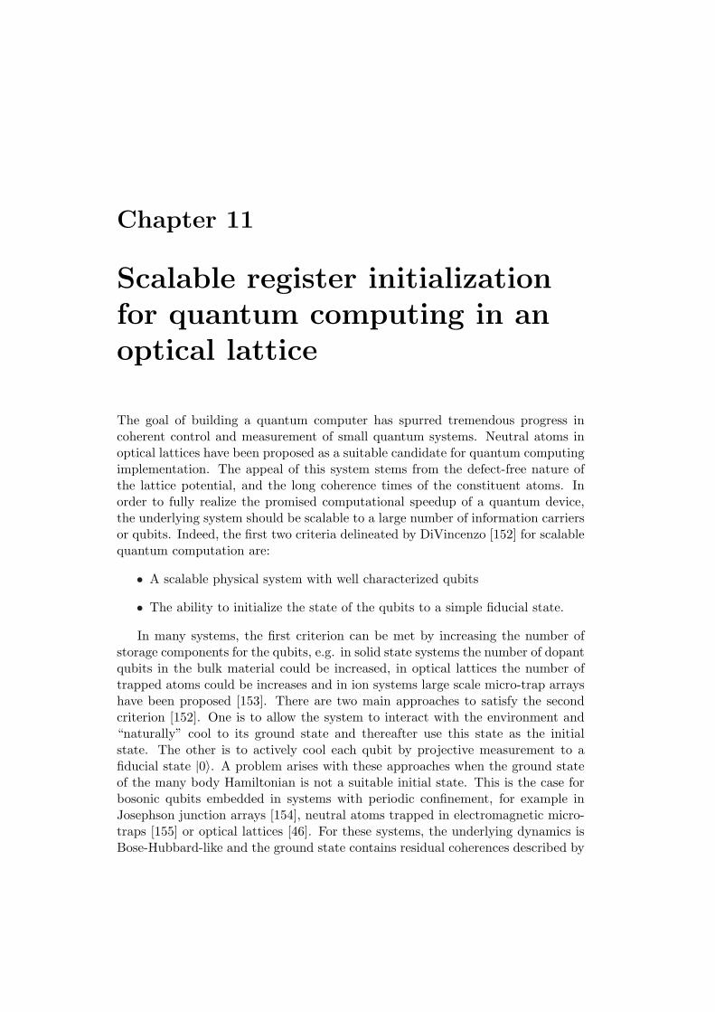
Chapter 11
Scalable register initializationfor quantum computing in anoptical lattice
The goal of building a quantum computer has spurred tremendous progress incoherent control and measurement of small quantum systems. Neutral atoms inoptical lattices have been proposed as a suitable candidate for quantum computingimplementation. The appeal of this system stems from the defect-free nature ofthe lattice potential, and the long coherence times of the constituent atoms. Inorder to fully realize the promised computational speedup of a quantum device,the underlying system should be scalable to a large number of information carriersor qubits. Indeed, the first two criteria delineated by DiVincenzo [152] for scalablequantum computation are:
• A scalable physical system with well characterized qubits
• The ability to initialize the state of the qubits to a simple fiducial state.
In many systems, the first criterion can be met by increasing the number ofstorage components for the qubits, e.g. in solid state systems the number of dopantqubits in the bulk material could be increased, in optical lattices the number oftrapped atoms could be increases and in ion systems large scale micro-trap arrayshave been proposed [153]. There are two main approaches to satisfy the secondcriterion [152]. One is to allow the system to interact with the environment and“naturally” cool to its ground state and thereafter use this state as the initialstate. The other is to actively cool each qubit by projective measurement to afiducial state |0〉. A problem arises with these approaches when the ground stateof the many body Hamiltonian is not a suitable initial state. This is the case forbosonic qubits embedded in systems with periodic confinement, for example inJosephson junction arrays [154], neutral atoms trapped in electromagnetic micro-traps [155] or optical lattices [46]. For these systems, the underlying dynamics isBose-Hubbard-like and the ground state contains residual coherences described by

194Chapter 11 Scalable register initialization for quantum computing in
an optical lattice
non-zero number fluctuations in each mode. As shown in Eq.(9.8), these fluctua-tions scale as gJ/U
√M , so if not corrected, the dynamics will impart a constraint
to scalability. In this chapter we show how this can be corrected in two steps,first by introducing an inhomogeneity to the lattice using a quadratic trappingpotential and second by projecting out components of the many-body wavefunc-tion with multiply occupied lattice sites by selective measurements on a molecularphoto-associative transition. Provided the measurement strength is sufficientlylarge, the system does not evolve out of the restricted basis and the measurementcan maintain a unit filled register for the duration of quantum computation. Thisstrategy allows the Mott insulator transition to become a robust mechanism forregister initialization.
11.1 Homogeneous dynamics
It was recognized early on that the Mott insulator transition might be an effi-cient way to initialize a register of atomic qubits in an optical lattice for use inquantum information processing. A key advantage of loading from a BEC is theavailability of an initially high phase space density which can be frozen to the Mottinsulator state with atoms occupying most lattice sites. For the homogeneous sys-tem (Vi = 0), only commensurate fillings give rise to a Mott insulator transition.For the purposes of quantum computation, one particle per well is desirable. Inpractice, this is difficult to achieve directly because the precise number of atomsis unknown and the lattice strength is not perfectly uniform on the boundaries.There are proposals to prepare unit filled lattices using dissipative techniques in-volving filling the lattice atom by atom [156] or using Raman side-band cooling[157]. Additionally, it has been shown that one can repair imperfect filling from aBEC via an adiabatic transfer mechanism between two sublevels of each atom [48].While these techniques can initialize the lattice, any mechanism used to prepare aregister of qubits in the unit filled state will suffer a degradation in fidelity, definedas the population in the unit filled state. The degradation comes from the couplingbetween the desired unit filled state and undesired states that pertain to the exactMott ground state.
In this section we derive the time dependent fidelity in a homogeneous com-mensurately filled system prepared at time t = 0 in the unit filled Fock state |T 〉(See Eq.(9.4)). While our results can be generalized to higher dimensions, we con-sider only a one dimension system. We assume an idealized homogeneous latticewith periodic boundaries and unit filling, g = N/M = 1, where N is the number ofatoms and M is the number of wells. The regime of interest is the strong couplinglimit, where first order perturbation theory is valid. This regime is experimentallyachievable in an optical lattice because the tunneling decreases exponentially withthe trap depth.
To study the time dependent fidelity at first order in perturbation theory, inprinciple we have to consider all the M(M −1) eigenmodes that span the one par-ticle hole subspace. However, by translational symmetry only the translationally
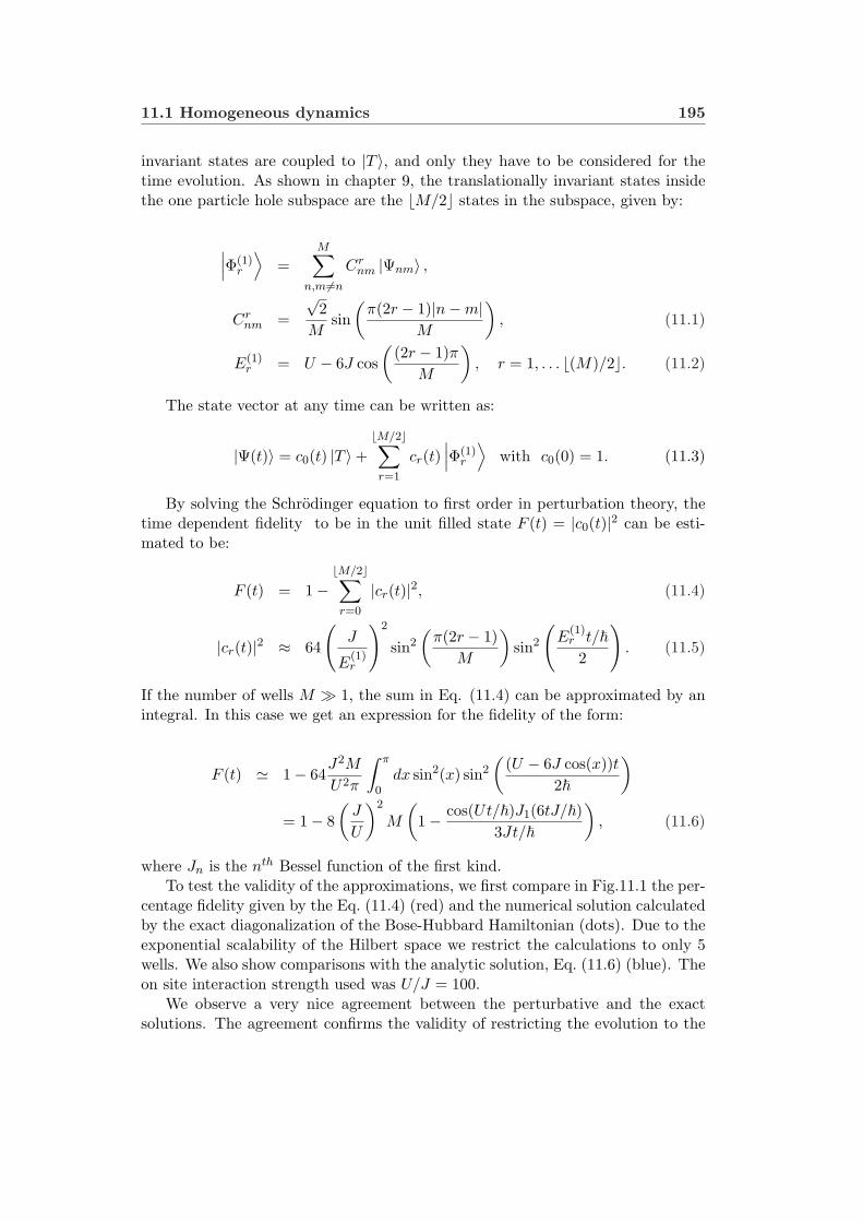
11.1 Homogeneous dynamics 195
invariant states are coupled to |T 〉, and only they have to be considered for thetime evolution. As shown in chapter 9, the translationally invariant states insidethe one particle hole subspace are the bM/2c states in the subspace, given by:
∣∣∣Φ(1)r
⟩=
M∑
n,m6=n
Crnm |Ψnm〉 ,
Crnm =
√2
Msin
(π(2r − 1)|n−m|
M
), (11.1)
E(1)r = U − 6J cos
((2r − 1)π
M
), r = 1, . . . b(M)/2c. (11.2)
The state vector at any time can be written as:
|Ψ(t)〉 = c0(t) |T 〉+bM/2c∑
r=1
cr(t)∣∣∣Φ(1)
r
⟩with c0(0) = 1. (11.3)
By solving the Schrodinger equation to first order in perturbation theory, thetime dependent fidelity to be in the unit filled state F (t) = |c0(t)|2 can be esti-mated to be:
F (t) = 1−bM/2c∑
r=0
|cr(t)|2, (11.4)
|cr(t)|2 ≈ 64
(J
E(1)r
)2
sin2
(π(2r − 1)
M
)sin2
(E
(1)r t/~2
). (11.5)
If the number of wells M À 1, the sum in Eq. (11.4) can be approximated by anintegral. In this case we get an expression for the fidelity of the form:
F (t) ' 1− 64J2M
U2π
∫ π
0dx sin2(x) sin2
((U − 6J cos(x))t
2~
)
= 1− 8(
J
U
)2
M
(1− cos(Ut/~)J1(6tJ/~)
3Jt/~
), (11.6)
where Jn is the nth Bessel function of the first kind.To test the validity of the approximations, we first compare in Fig.11.1 the per-
centage fidelity given by the Eq. (11.4) (red) and the numerical solution calculatedby the exact diagonalization of the Bose-Hubbard Hamiltonian (dots). Due to theexponential scalability of the Hilbert space we restrict the calculations to only 5wells. We also show comparisons with the analytic solution, Eq. (11.6) (blue). Theon site interaction strength used was U/J = 100.
We observe a very nice agreement between the perturbative and the exactsolutions. The agreement confirms the validity of restricting the evolution to the
196Chapter 11 Scalable register initialization for quantum computing in
an optical lattice
0 0.5 1 1.5 2 2.5t JÑ
99.2
99.4
99.6
99.8
100
%Fi
delit
y
M=5, g=1 ,!!!!!!
M JU=0.02
Figure 11.1: Comparisons between the time evolution of the percentage fidelitycalculated by diagonalizing the Bose-Hubbard Hamiltonian (dots), the perturba-tive solution inside the one particle hole subspace (red) and the analytic solutionEq. 11.6 (blue).
one particle hole subspace. On the other hand, because of the small number ofwells used for the simulations, we do not expect Eq. (11.6) to be a very goodapproximation. Nevertheless, we observe that for short times the analytic solutionis a fair description of the dynamics.
In Fig.11.2 we compare the analytic solution, Eq. (11.6) (blue) with the pertur-bative solution given by Eq. (11.4) (red) for a larger system with M = 31. Eventhough for this large number of wells an exact solution is not available, we ensurethe validity of perturbation theory by choosing the same
√MJ/U than the one in
Fig.11.1. In this M = 31 case, which lies in a regime where we expect Eq. (11.6)to be valid, the agreement between the blue and red curves is very good.
In general the behavior of F (t) consists of fast oscillations with frequency equalto U/~, modulated by longer oscillations with frequency determined by the zerosof J1. For short times, Jt/~¿ 1, the fidelity is
F (t) ≈ 1− 16(
J
U
)2
M sin2
(Ut/~
2
), (11.7)
which corresponds to the Rabi oscillations of an effective two level system spannedby |T 〉 and |S〉, with |S〉 the translationally invariant state directly coupled to thefirst order ground state (see Eq. (9.9)). For later times the coupling to otherstates becomes important. Notice that the time average of the fidelity over manyoscillation periods is 〈F (t)〉 = 1− 8(J/U)2M . Consequently, the deviation from a
11.2 Dynamics in presence of the external trap 197
0 0.5 1 1.5 2t JÑ
99.2
99.4
99.6
99.8
100%
Fide
lity
M=31, g=1 ,!!!!!!
M JU=0.02
Figure 11.2: Percentage fidelity as a function of time calculated using the pertur-bative solution 11.4 (red) and the analytic solution Eq. 11.6 (blue).The numberof sites used for the plot is M = 31
perfectly prepared register, described by 1−〈F (t)〉, is twice as bad as if the systemwere prepared in the stationary ground state of the Bose-Hubbard Hamiltonian(Eq. (9.8)). This indicates that a lattice filled with a commensurate number ofatoms in the Mott insulator state may create a more robust quantum computerregister than one prepared dissipatively.
11.2 Dynamics in presence of the external trap
As mentioned before, in practice it is difficult to prepare an optical lattice withexactly one atom per well. To arrange the desired configuration, we propose touse an inhomogeneous lattice with open boundaries created by a weak quadraticmagnetic trap. We require fewer number of atoms than available sites, N < M .The addition of the trap acts to collect atoms near the potential minimum andleaves empty wells (holes) at the edges. In experiments where the optical lattice isloaded from a BEC, the external trap is already present to confine the condensate.For simplicity we assume a one dimensional trap with oscillation frequency givenby ωT . The magnetic confinement introduces a characteristic energy scale Ω =m/2a2ωT , so that Vn = Ωn2 (see Eq. (6.1)). To inhibit multiple atom occupationin any well in the ground state configuration, we require the on site interactionenergy U to be larger than the trapping energy of the most externally trappedatoms, U > Ω(N−1)2
4 .

198Chapter 11 Scalable register initialization for quantum computing in
an optical lattice
Figure 11.3: Schematic of an inhomogeneous lattice filled with N qubits with anonsite interaction energy U . An externally applied trapping potential of strengthVj = Ωj2, e.g. due to a magnetic field, acts to fill gaps in the central region of thetrap. The center subspace R of the lattice defines the quantum computer registercontaining K < N qubits.
We define our register as the subspace R comprising K < N wells in thecenter region of the the trap (see Fig. 11.3). The barrier space flanking R willact to suppress percolation of holes from the edges to the center. The esti-mated probability for holes in R due to tunneling through the barrier is ph ≈∏(N+1)/2
j=(K−1)/2(J/Ω(2j + 1))2 = (J/2Ω)N−K+4(Γ[K/2]/Γ[N/2 + 1])2, which is negli-gible provided the barrier region is sufficiently large and J/KΩ < 1.
Hereafter, we restrict our attention to the dynamics of the reduced state of theregister obtained by the tracing over spatial modes outside the register subspaceof the entire many body wavefunction. The degree of inhomogeneity is quantifiedby the ratio Ω/J . For 0 < Ω/J ¿ 1, the energy splitting between Fock statesdescribing particle-hole pairs is small and the model of homogeneous dynamics isvalid.
For Ω/J & 1, to first order in perturbation theory, the state space is spannedby the unit filled state in the register subspace, |T 〉R, and the 2K nearest neighborparticle-hole pairs |S±j 〉:
|T 〉R = |1, 1, 1, . . . , , 1, 1, 1〉︸ ︷︷ ︸K sites
, (11.8)
|S+j 〉R = |1, . . . , 2︸︷︷︸
j
, 0︸︷︷︸j+1
, . . . , 1〉. |j| < (K − 1)/2, (11.9)
|S−j 〉R = |1, . . . , 2︸︷︷︸j−1
, 0︸︷︷︸j
, . . . , 1〉. (11.10)
Here we have introduced coordinates with the site j = 0 coincident with the trapminimum. For each j the states |S±j 〉R are distinguished by the two energeticallydistinct orientations of a doubly occupied site and its neighboring hole with ener-gies, E(S±j ) = U(1∓ Ω
U (2j − 1)). We define the zero of energy coincident with thestate |T 〉R.

11.2 Dynamics in presence of the external trap 199
With an eye to the projective measurement, it is important to understand thefree dynamics when the trap is present and the register is initialized in the purestate |T 〉R inside the register, R〈T |Ψ(0)〉R = 1. Here |Ψ(0)〉R is the projectionof the initial many body state |Ψ(0)〉 in the register subspace, i.e. |Ψ(0)〉R =|P〉〈P|Ψ(0)〉 with |P〉〈P| the projection operator that traces over spatial modesoutside the register. We proceed to estimate the fidelity to be in the unit filledstate in the register: FR(t) = |R〈T |P〉〈|P|Ψ(t)〉|2 ≡ |R〈T |Ψ(t)〉R|.
The quantity FR(t) is generally difficult to compute because atoms couple intoand out of the register. Instead, we will first solve the simpler problem of thefidelity to be in the target state of a commensurately filled inhomogeneous latticewith K sites. We will use this fidelity to estimate FR(t). In the commensuratelyfilled inhomogeneous system, to first order in J/U , the dynamics can be restrictedto the Hilbert space spanned by the state vectors |T 〉R, |S±j 〉R, and therefore thetime dependent state can be written as :
|Ψ(t)〉com = cT (t)|T 〉R +∑
j,±e−iE(S±j )t/~cS±j
(t)|S±j 〉R. (11.11)
The evolution of the amplitudes cT (t), cS±j(t) is dictated by the following equa-
tions of motion:
i~∂
∂tcT (t) = −J
√2
∑
j,±e−iE(S±j )t/~cS±j
(t), (11.12)
i~∂
∂tcS±j
(t) = −J√
2e−iE(S±j )t/~cT (t). (11.13)
Using the fact that J/U ¿ 1, for times Jt . ~ we can set the value of cT (t) in Eq.(11.13) to 1. Integrating the equation we obtain
|cS±j(t)|2 = 8
(J
U
)2
sin2
(E(S±j )t
2~
), (11.14)
|cT (t)|2 = 1− 8(
J
U
)2 ∑
j,±
∣∣∣cS±j(t)
∣∣∣2. (11.15)
After performing the sum, the fidelity Fcom(K, t) ≡ |cT (t)|2 is :
Fcom(K, t) ≈ 1− 8J2
U2
(K − cos(Ut/~)
(1 +
sin(Ω(K − 1)t/~)sin(Ωt/~)
)). (11.16)
Notice that for Ωt → 0, we recover the short time fidelity in the homogeneous case,Eq. (11.7).
Once Fcom(K, t) is calculated, we can bound the fidelity FR(t) inside the reg-ister. Provided N > K the following inequalities on the time averaged fidelitieshold:
〈Fcom(N, t)〉 ≤ 〈FR(t)〉 ≤ 〈Fcom(K, t)〉. (11.17)

200Chapter 11 Scalable register initialization for quantum computing in
an optical lattice
The lower bound arises because the probability to be in the unit filled state ofa large commensurately filled lattice, given an initial state which is unit filled, isalways less than or equal to the probability to be unit filled over a smaller subspaceof K < N of a non commensurately filled lattice whose register is prepared in theunit filled state. This inequality holds provided the probability for holes to tunnelinto the register R is small over relevant time scales. The upper bound is aconsequence of the fact that unit filling in the register state is degraded becauseparticles can tunnel in and out of the register. Therefore its fidelity is less thanthat of a commensurately filled lattice of the same size K prepared in the unitfilled state.
0 0.5 1 1.5 2t JÑ
99.2
99.4
99.6
99.8
100
%F c
omHK=
5,tL
g=1 ,UJ=100, WJ=2.7
Figure 11.4: Comparisons between the time evolution of the percentage fidelityFcom(K = 5, t) calculated by evolving the initial target state using the Bose-Hubbard Hamiltonian (dots), the restricted one particle hole basis (red) and theanalytic solution Eq. 11.16 (blue). In the plot we assumed a commensurate unitfilled lattice with five sites and infinitely high boundaries.
In Fig. 11.4 we compare this analytic solution, Eq. 11.16 (blue), with the solutionsfound by propagating the initial state using the exact Bose-Hubbard Hamiltonian(dots) and by using a restricted basis set of dimension K(K − 1) + 1 consistingof the target state and all particle-hole pairs (red). Infinitely high boundarieswere assumed for the numerical solutions. The parameters used for the plot wereU/J = 100,Ω/J = 2.7 and K = 5. We observe complete agreement between theexact points and the red curve, which justifies the restriction of the dynamics tothe one-particle hole subspace. On the other hand, the analytic approximationaccurately reproduces the exact dynamics only for times t . 0.5~/J . This is notunexpected because the analytic solution only takes into account the states with
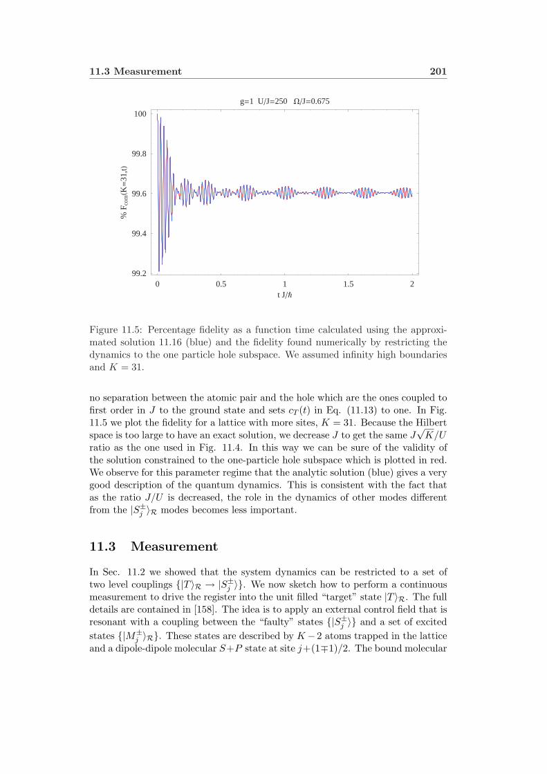
11.3 Measurement 201
0 0.5 1 1.5 2t JÑ
99.2
99.4
99.6
99.8
100%
F comHK=
31,tL
g=1 UJ=250 WJ=0.675
Figure 11.5: Percentage fidelity as a function time calculated using the approxi-mated solution 11.16 (blue) and the fidelity found numerically by restricting thedynamics to the one particle hole subspace. We assumed infinity high boundariesand K = 31.
no separation between the atomic pair and the hole which are the ones coupled tofirst order in J to the ground state and sets cT (t) in Eq. (11.13) to one. In Fig.11.5 we plot the fidelity for a lattice with more sites, K = 31. Because the Hilbertspace is too large to have an exact solution, we decrease J to get the same J
√K/U
ratio as the one used in Fig. 11.4. In this way we can be sure of the validity ofthe solution constrained to the one-particle hole subspace which is plotted in red.We observe for this parameter regime that the analytic solution (blue) gives a verygood description of the quantum dynamics. This is consistent with the fact thatas the ratio J/U is decreased, the role in the dynamics of other modes differentfrom the |S±j 〉R modes becomes less important.
11.3 Measurement
In Sec. 11.2 we showed that the system dynamics can be restricted to a set oftwo level couplings |T 〉R → |S±j 〉. We now sketch how to perform a continuousmeasurement to drive the register into the unit filled “target” state |T 〉R. The fulldetails are contained in [158]. The idea is to apply an external control field that isresonant with a coupling between the “faulty” states |S±j 〉 and a set of excitedstates |M±
j 〉R. These states are described by K− 2 atoms trapped in the latticeand a dipole-dipole molecular S+P state at site j+(1∓1)/2. The bound molecular
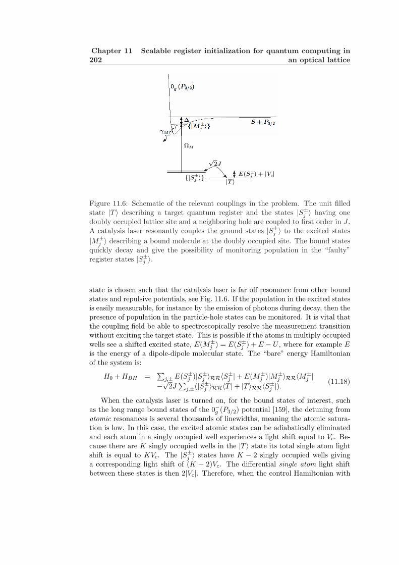
202Chapter 11 Scalable register initialization for quantum computing in
an optical lattice
|T 〉|S±
j 〉
√
2J
0−
g (P3/2)
|M±j 〉
∆
γM
S + P3/2
E(S±j) + |Vc|
ΩM
Figure 11.6: Schematic of the relevant couplings in the problem. The unit filledstate |T 〉 describing a target quantum register and the states |S±j 〉 having onedoubly occupied lattice site and a neighboring hole are coupled to first order in J .A catalysis laser resonantly couples the ground states |S±j 〉 to the excited states|M±
j 〉 describing a bound molecule at the doubly occupied site. The bound statesquickly decay and give the possibility of monitoring population in the “faulty”register states |S±j 〉.
state is chosen such that the catalysis laser is far off resonance from other boundstates and repulsive potentials, see Fig. 11.6. If the population in the excited statesis easily measurable, for instance by the emission of photons during decay, then thepresence of population in the particle-hole states can be monitored. It is vital thatthe coupling field be able to spectroscopically resolve the measurement transitionwithout exciting the target state. This is possible if the atoms in multiply occupiedwells see a shifted excited state, E(M±
j ) = E(S±j ) + E − U , where for example Eis the energy of a dipole-dipole molecular state. The “bare” energy Hamiltonianof the system is:
H0 + HBH =∑
j,±E(S±j )|S±j 〉RR〈S±j |+ E(M±j )|M±
j 〉RR〈M±j |
−√2J∑
j,±(|S±j 〉RR〈T |+ |T 〉RR〈S±j |).(11.18)
When the catalysis laser is turned on, for the bound states of interest, suchas the long range bound states of the 0−g (P3/2) potential [159], the detuning fromatomic resonances is several thousands of linewidths, meaning the atomic satura-tion is low. In this case, the excited atomic states can be adiabatically eliminatedand each atom in a singly occupied well experiences a light shift equal to Vc. Be-cause there are K singly occupied wells in the |T 〉 state its total single atom lightshift is equal to KVc. The |S±j 〉 states have K − 2 singly occupied wells givinga corresponding light shift of (K − 2)Vc. The differential single atom light shiftbetween these states is then 2|Vc|. Therefore, when the control Hamiltonian with
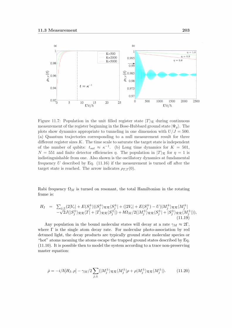
11.3 Measurement 203
Figure 11.7: Population in the unit filled register state |T 〉R during continuousmeasurement of the register beginning in the Bose-Hubbard ground state |Ψg〉. Theplots show dynamics appropriate to tunneling in one dimension with U/J = 500.(a) Quantum trajectories corresponding to a null measurement result for threedifferent register sizes K. The time scale to saturate the target state is independentof the number of qubits: tsat ≈ κ−1. (b) Long time dynamics for K = 501,N = 551 and finite detector efficiencies η. The population in |T 〉R for η = 1 isindistinguishable from one. Also shown is the oscillatory dynamics at fundamentalfrequency U described by Eq. (11.16) if the measurement is turned off after thetarget state is reached. The arrow indicates ρT,T (0).
Rabi frequency ΩM is turned on resonant, the total Hamiltonian in the rotatingframe is:
HI =∑
j,±(2|Vc|+ E(S±j ))|S±j 〉RR〈S±j |+ (|2Vc|+ E(S±j )− U)|M±j 〉RR〈M±
j |−√2J(|S±j 〉RR〈T |+ |T 〉RR〈S±j |) + ~ΩM/2(|M±
j 〉RR〈S±j |+ |S±j 〉RR〈M±j |)),
(11.19)
Any population in the bound molecular states will decay at a rate γM ≈ 2Γ,where Γ is the single atom decay rate. For molecular photo-association by reddetuned light, the decay products are typically ground state molecular species or“hot” atoms meaning the atoms escape the trapped ground states described by Eq.(11.10). It is possible then to model the system according to a trace non-preservingmaster equation:
ρ = −i/~[HI , ρ]− γM/2∑
j,±(|M±
j 〉RR〈M±j |ρ + ρ|M±
j 〉RR〈M±j |). (11.20)

204Chapter 11 Scalable register initialization for quantum computing in
an optical lattice
Assuming low saturation of the excited states, the dynamics in the ground state is
ρS±j ,T = −iρS±j ,T (E(S±j ) + |Vc|)/~+ i(ρT,T − ρS±j ,S±j)√
2J/~− ρS±j ,T κ
ρT,T = i(ρS±j ,T − ρT,S±j)√
2J/~ρS±j ,S±j
= −i(ρS±j ,T − ρT,S±j)√
2J/~− 2ρS±j ,S±jκ.
(11.21)These equations describe the Bose-Hubbard coupled states with a decay in
population of each state with an atomic pair at a rate 2κ = ΩM2γM/(4(U/~)2 +
(γM/2)2), and decay of coherences between each of these states and state |T 〉 at arate κ.
This type of evolution characterized by measurement induced phase dampingwas studied extensively by Gagen and Milburn [160]. We now show that our systemcan satisfy the conditions for this effect and in particular can be driven to the |T 〉state by monitoring the environment for a signature of decay from the molecularbound state.
For the inhomogeneous system, the state |T 〉 couples to 2K distinguishablestates |S±j 〉. However, we can define an effective Rabi frequency between the state|T 〉 and the subspace spanned by |S±J 〉. This frequency is close to the couplingmatrix element between the state |T 〉 and the state |S〉 in the homogeneous system,namely 2
√KJ . The coherences between the two subspaces decay at a rate κ,
and the population in the subspace |S±j 〉 decays at a rate 2κ. The “good”measurement regime as derived in [160] is then:
ΩM/γM ¿ 1 < ~κ/2√
KJ. (11.22)
The left side inequality ensures that the excited states |M±j 〉 are weakly pop-
ulated (equivalent to the condition for adiabatic elimination of these states). Theright side inequality ensures that measurement is sufficiently strong to damp co-herences on the time scale that they develop due to tunneling.
When the environment is monitored, for instance by looking for photon scatter-ing from the bound molecular state, the evolution of ground states can be modelledusing quantum trajectories. The success or failure of the preparation is conclusivewith failure probability pfail = 1− ρT,T (0). Real experiments will be constrainedto finite detector efficiencies η. For η = 0, corresponding to nonselective measure-ment, the system dynamics evolve according to Eq. (11.21). In the case of finitedetector efficiencies, we can express the approximate fidelity to be in the targetstate is F (η, t) = ρT,T (t) = η + (1 − η)ρη=0
T,T (t). Simulations of successful registerpreparation and maintenance by measurement with different efficiencies are shownin Fig. 11.7.
It is necessary to keep the measurement on during a computation to maintainhigh fidelity in the unit filled state. If instead the catalysis field is turned off afterthe target state is reached, the system will freely evolve as shown in Sec. 11.2.To illustrate this we show in Fig. 11.7 the evolution of the fidelity described byEq. (11.16) if the measurement is turned off after the target state is reached.
11.4 Conclusions 205
11.4 Conclusions
In summary, we have shown that efforts to prepare a register of atomic qubits in anoptical lattice suffer from errors inherent in the underlying many body dynamics.By considering the free dynamics in both homogeneous and trapped systems wehave shown that there is a loss of fidelity of initialization of the unit filled regis-ter which scales with the number of qubits because it is not a stationary state.Because our analysis is based on first order perturbation theory we establishedthe parameter regime where our analytic approach is valid by comparing it withexact numerical results for moderate numbers of atoms and wells. To make theMott insulator transition a robust mechanism for initialization, we have suggestedone approach to correct for the mentioned problems by performing a continuousmeasurement on the system. While our discussion has focused on one dimensionaldynamics, the method is also applicable to higher dimensions, which is the relevantregime for scalability.

206Chapter 11 Scalable register initialization for quantum computing in
an optical lattice
Chapter 12
Conlusions
This thesis gives a global understanding of the basic physics that describes bosoniccold atoms in optical lattices, starting from the superfluid regime and going intothe strongly correlated Mott insulator regime. In the following I am going tosummarize what I consider are the most relevant contributions of this work.
• The equilibrium properties of lattice systems in the superfluid regime werestudied by using standard mean field techniques and quadratic approxima-tions.
• An explicit expression for the superfluid density based on the rigidity of thesystem under phase variations was derived. This expression enabled us toexplore the connection between the quantum depletion of the condensateand the quasimomentum distribution on the one hand, and the superfluidfraction on the other. Also, the superfluid fraction was shown to be a naturalorder parameter to describe the superfluid to Mott insulator transition.
• A functional effective action approach, the 2PI-CTP formalism, capable ofdealing with nonequilibrium situations that require a treatment beyond meanfield theory, was studied. Using the patterned loading system, this formalismwas shown to be a powerful tool to go beyond the HFB approximation andto incorporate the nonlocal and non-Markovian aspects characteristic of thequantum dynamics.
• It was shown that the complicated nonlocal and non-Markovian solutionsderived using the 2PI-CTP formalism reduce to the standard kinetic theoryequations when the system dynamics admits two-time separation.
• Bragg spectroscopy was shown to be a suitable experimental tool to char-acterizing the Mott insulator phase and to estimate the temperature of thesystem deep in the Mott insulator regime.
• It was shown that the use of a lattice with a spatial inhomogeneity createdby a quadratic magnetic trapping potential, together with a selective mea-
208 Chapter 12 Conlusions
surement of atomic pairs allow for the Mott insulator transition to becomea robust mechanism for quantum register initialization.
In the recent years there has been spectacular progress in experimental and the-oretical studies of atoms loaded into an optical lattice. However, there are stillmany ideas and possible experiments that could help us to address fundamen-tal questions in solid state physics, atomic physics, quantum optics and quantuminformation. I want to finish this work by mentioning some of them.
One can use for example multi-component ultracold atoms in optical latticestogether with Feshbach resonances to realize Hamiltonians other than the pureBose-Hubbard one. Also by loading fermionic atoms into an optical lattice theHubbard Hamiltonian could be realized. This could help to answer many theo-retical questions still open in fermionic systems, such as the BEC-BCS crossoverand the basic physics behind high temperature superconductivity. From the per-spective of atomic and molecular physics an interesting experiment could be theuse of the Mott insulator state with two atoms per site as a mean to create amolecular condensate. The creation of vortices in individual lattice sites couldalso allow the study of the integer and fractional quantum Hall effects in ultracoldgases. By introducing noise in a controlled way in optical lattice, one can alsostudy disordered periodic systems, which are very important in condensed matterphysics. And finally and perhaps one of the most challenging tasks is to developthe necessary techniques and protocols that allow neutral atoms in optical latticesas a mean to implement a quantum computer.

Bibliography
[1] A. Einstein, Sitzungsbericht der Preussischein Akademie der Wissenschaften,p. 3,(1925).
[2] S. N. Bose Z. Phys 26, 178(1924).
[3] F. London, Nature 141, 643 (1938); Phys. Rev 54, 947 (1938).
[4] E. C. Svensson and V. F. Sears, Progress of low temperature physics, Vol XI,ed. D.F. Brewer, (North Holland,Amsterdam,187).
[5] I. F. Silvera and J. T. M. Walraven, Phys. Rev. Lett 44, 164 (1980).
[6] M. H. Anderson, J. R. Ensher, M. R. Matthewes, C. E. Wieman and E. A.Cornell Science 269, 198 (1995).
[7] K. B. Davis, M. O. Mewes, M. R. Andrews, N. J. van Druten, D. S. Durfee,D. M. Kurn and W. Ketterle, Phys. Rev. lett. 75, 3969 (1995).
[8] C. C. Bradley, C. A. Sackett, J. J. Tollet and R. Hulet, Phys. Rev. Lett. 78,985 (1997).
[9] C. J. Foot, Contemp. Phys. 32, 369 (1991).
[10] E. P. Gross, Nuovo Cimiento, 20, 454 (1961); L. P. Pitaevskii, Sov. Phys.JETP 13, 451 (1961).
[11] N. N. Bogoliubov, J. Phys. (USSR) 11, 23 (1947).
[12] F. Dalfovo, S. Giorgini, L. P. Pitaevskii and S. Stringari, Theory of Bose-Einstein condensation in trapped gases, Rev. Mod. Phys. 71, 463 (1999).
[13] D. A. W. Hutchinson et al., J. Phys. B: At. Mol. Opt. Phys. 57 3825 (2000).
[14] N.P. Proukakis, S.A. Morgan, S. Choi and K. Burnett, Phys. Rev. A 58, 2435(1998).
[15] H. Shi and A. Griffin, Phys. Rep. 304, 1 (1998) and A. Griffin, Phys. Rev. B,53, 9341 (1995).
210 BIBLIOGRAPHY
[16] S. A. Morgan A gapless theory of Bose-Einstein Condensation in Dilute Gasesat Finite Temperature, D. Phil. Thesis, Oxford University (1999), S. A. Mor-gan, J. Phys. B: At. Mol. Opt. Phys. 57, 3847 (2000).
[17] D. S. Jin, J. R. Ensher, M. R. Matthews, C. E. Wieman and E. A. Cornell,Phys. Rev. Lett. 77, 420 (1996).
[18] S. Stringari Phys. Rev. Lett. 77, 2360 (1996); F. Dalfovo, S. Giorgini, M.Guilleumas, L. Pitaevskii, and S. Stringari, Phys. Rev. A 56, 3840 (1997).
[19] M. Edwards, R. J. Dodd, C. W. Clark, P. A. Ruprecht and K. Burnett, Phys.Rev. A 53, R1950 (1996); M. Edwards, P. A. Ruprecht, K. Burnett, R. J.Dodd and C. W. Clark, Phys. Rev. Lett. 77, 1671 (1996); M. Rusch and K.Burnett, Phys. Rev. A 59, 3851 (1999); D. A. W. Hutchinson, E. Zaremba andA. Griffin, Phys. Rev. Lett. 78, 1842 (1997); L. P. Pitaevskii and S. Stringari,Phys. Lett. A 235, 398 (1997); R. J. Dodd, M. Edwards, C. W. Clark and K.Burnett, Phys. Rev. A, 57, R32 (1998).
[20] S. L. Cornish, N. R. Claussen, J. L. Roberts, E. A. Cornell, and C. E. WiemanPhys. Rev. Lett. 85, 1795 (2000).
[21] Elizabeth A. Donley, Neil R. Claussen, Simon L. Cornish, Jacob L. Roberts,Eric A. Cornell, Carl E. Wieman, Nature 412, 295 (19 Jul 2001).
[22] P. O. Fedichev, M. W. Reynolds, and G. V. Shlyapnikov, Phys. Rev. Lett.77, 2921 (1996).
[23] Phillip L. Gould, George A. Ruff, and David E. Pritchard, Phys. Rev. Lett.56, 827 (1986).
[24] P. J. Martin, Bruce G. Oldaker, Andrew H. Miklich, and David E. Pritchard,Phys. Rev. Lett. 60, 515 (1988).
[25] C.S. Adams, M. Sigel and J. Mlynek, Phys. Rep 240, 143 (1994).
[26] A. Hemmerich and T. W. Hansch, Phys. Rev. Lett. 70, 410 (1993).
[27] A. Hemmerich, M. Weidemuller, T. Esslinger, C. Zimmermann, and T. Hn-sch,Phys. Rev. Lett. 75, 37 (1995).
[28] M. Weidemller, A. Hemmerich, A. Gorlitz, T. Esslinger, and T. W. Hansch,Phys. Rev. Lett. 75, 4583 (1995).
[29] G. Grynberg, B. Lounis, P. Verkerk, J. Y. Courtois, and C. Salomon, Phys.Rev. Lett. 70, 2249 (1993).
[30] Vladan Vuletic, Cheng Chin, Andrew J. Kerman, and Steven Chu, Phys. Rev.Lett. 81, 5768 (1998).
BIBLIOGRAPHY 211
[31] Andrew J. Kerman, Vladan Vuletic, Cheng Chin, and Steven Chu, Phys. Rev.Lett. 84, 439442 (2000).
[32] Marshall T. DePue, Colin McCormick, S. Lukman Winoto, Steven Oliver,and David S. Weiss, Phys. Rev. Lett. 82, 2262 (1999).
[33] S. Peil, J. V. Porto, B. L. Tolra et. al, Phys. Rev. A 67, 051603 (2003).
[34] P. Blair Blakie and Charles W. Clark, J. Phys. B: At. Mol. Opt. Phys. 371391 (2004).
[35] M. Greiner, I. Bloch, O. Mandel, T. W. Hansch, and T. Esslinger, Phys. Rev.Lett. 87, 160405 (2001).
[36] J. H. Denschlag, J. E. Simsarian, H. Haffner, C. McKenzie, A. Browaeys,D. Cho, K. Helmerson, S. L. Rolston, and W. D. Phillips, J. Phys. B 35, 3095(2002).
[37] F. Ferlaino, P. Maddaloni, S. Burger, F. S. Cataliotti, C. Fort, M. Modugno,and M. Inguscio Phys. Rev. A 66, 011604 (2002).
[38] O. Morsch, J. H. Muller, M. Cristiani, D. Ciampini, and E. Arimondo, Phys.Rev. Lett. 87, 140402 (2001).
[39] B. Anderson and M. Kasevich, Science 282, 1686 (1998).
[40] O. Morsch, M. Cristiani, J. H. Muller, D. Ciampini, and E. Arimondo, Phys.Rev. A 66, 021601 (2002).
[41] S. Burger, F. S. Cataliotti, C. Fort, F. Minardi, M. Inguscio, M. L. Chiofalo,and M. P. Tosi, Phys. Rev. Lett. 86, 4447 (2001).
[42] W. K. Hensinger, H. Haffner, A. Browaeys, N. R. Heckenberg, K. Helmerson,C. McKenzie, G. J. Milburn, W. D. Phillips, S. L. Rolston, H. Rubinsztein-Dunlop, Nature 412, 52 (2001).
[43] D. Jaksch, C. Bruder, C. W. Gardiner, J.I. Cirac and P. Zoller, Phys. Rev.Lett. 81, 3108 (1998).
[44] M. P. A. Fisher, P. B. Weichman, G. Grinstein and D. S. Fisher, Phys. Rev.B 40, 546 (1989).
[45] C. Orzel, A. K. Tuchman, M. L. Fenselau, M. Yasuda, and M. A. Kasevich,Science 23, 2386 (2001).
[46] M. Greiner, O. Mandel, T. Esslinger, T. W. Hansch, and I. Bloch, Nature415, 39 (2002).
[47] Markus Greiner, Olaf Mandel, Theodor W. Hansch and Immanuel Bloch,Nature 419, 51 (2002).
212 BIBLIOGRAPHY
[48] P. Rabl et al., Phys. Rev. Lett. 91, 110403 (2003).
[49] I. Deutsch et al., Phys. Rev. A 57, 1972 (1998).
[50] T. Calarco et al., J. Mod. Opt. 47, 2137 (2000).
[51] A. L. Fetter and J. D. Walecka,Quantum Theory of Many Particle Systems,(McGraw-Hill, New York, 1971).
[52] V. N. Popov, Functional Integrals in Quantum Field Theory and StatisticalPhysics (Reidel, Dordrecht, 1983).
[53] M. Bijlsma and H. T. C. Stoof, Phys. Rev. A 55, 498 (1997); U. Al Khawaja,J. O. Andersen, N. P. Proukakis, and H. T. C. Stoof Phys. Rev. A 66, 013615(2002).
[54] H. T. C. Stoof,in Coherent Matter Waves, proceedings of the summer LesHouches Lectures, session 72,1999, (Sprinder-Verlag, Berlin, 2001).
[55] Emil Lundl and Jorgen Rammer, Phys. Rev. A 66, 033607 (2002).
[56] J. S. Schwinger, J. Math. Phys. 2, 407 (1961); L. V. Keldysh, Zh. Eksp. Teor.Fiz. 47 , 1515 (1964) [Engl. trans. Sov. JETP 20 1018 (1965)]; V. Korenman,Ann. Phys. 39, 72 (1966); G. Zhou, Z. Su, B. Hao and L. Yu, Phys. Rep. 118,1 (1985).
[57] J. Luttinger and J. Ward, Phys. Rev. 118, 1417 (1960); C. de Dominicisand P. Martin, J. Math. Phys. 5, 14 (1964); H.D. Dahmen and G. JonaLasino, Nuovo Cimiento, 52A, 807 (1962); J.M. Cornwall, R. Jackiw and E.Tomboulis, Phys. Rev. D 10 2428 (1974).
[58] R. Walser, J. Williams, M. J. Holland et al., Phys. Rev. A 59, 3878(1999); R.Walser, J. Cooper and M. Holland, Phys. Rev. A 63, 013607 (2000).
[59] J. Wachter, R. Walser, J. Cooper and M. Holland, Phys. Rev. A 64,053612(2001).
[60] M. Imamovi-Tomasovi and A. Griffin, in Progress in Nonequilibrium Green’sFunctions, edited by M. Bonitz (World Scientific, Singapore, 2000), p. 404;M. Imamovi-Tomosovi and A. Griffin, Phys. Rev. A 60, 494 (1999).
[61] S. G. Bhongale, R. Walser and M. J. Holland Phys. Rev. A 66, 043618 (2002).
[62] J. Wachter, R. Walser, J. Cooper, and M. Holland Phys. Rev. A 65,039904 (2002); J. Wachter, R. Walser, J. Cooper, M. Holland, arXiv:cond-mat/0212432.
[63] S. T. Beliaev, Zh. Eksp. Teor. Fiz. 34, 433 (1958) [Sov. Phys. JETP 7, 299(1958)].
BIBLIOGRAPHY 213
[64] B. Paredes et al., Nature 429, 277 (2004).
[65] J. Stenger et al., Phys. Rev. Lett. 82, 4569 (1999).
[66] D. Stamper-Kurn et al., Phys. Rev. Lett. 83, 2876 (1999).
[67] N. W. Ashcroft and N. D. Mermin, Solid State Physics, W. B. SaundersCompany (1976).
[68] J. M. Ziman, Principles of the Theory of Solids, Cambridge University Press,(1964).
[69] I. Abramowitz and I. A. Stegun, Handbook of Mathematical Functions (Na-tional Bureau of Standards, 1964).
[70] Hidestoshi Fukuyama, Phys. Rev. B, 8, 5579 (1973).
[71] G. Wannier, Phys. Rev. 17, 432 (1960).
[72] Gerhard Fasol, Spectroscopy of Semiconductor Microstructures, (NATO ASISeries, 1989, p. 333)
[73] M. BenDahan, E. Peik, J. Reichel, Y. Castin, and C. Salomon, Phys. Rev.Lett. 76, 4508 (1996).
[74] W. Krauth, et al. Phys. Rev. B 45, 3137 (1992).
[75] K. Seshadri et al, Europhys. Lett. 22, 257 (1993).
[76] L. Amico and V. Penna, Phys. Rev. B 62, 1224 (2000).
[77] D. van Oosten, P. van der Straten, and H. T. C. Stoof, Phys. Rev. A 63,053601 (2001).
[78] J. K. Freericks and H. Monien, Phys. Rev. B 53, 2691 (1996).
[79] G. G. Batrouni et al. Phys. Rev. Lett. 65, 1765 (1990); R. T. Scalettar etal., Phys. Rev. Lett. 66, 3144 (1991); P. Niyaz et al., Phys. Rev. B. 44, 7143(1991); R. T. Scalettar et al., Phys. Rev. Lett. 74, 2527 (1995); G. G. Batrouniet al., Phys. Rev. Lett. 89, 117203 (2002).
[80] P. W. Anderson, Rev. Mod. Phys. 38, 298 (1966); A. J. Leggett, Rev. Mod.Phys. 73, 307 (2001); A. J. Leggett and F. Sols, Found. Phys. 31, 353 (1991).
[81] V. L. Ginzburg and L. D. Landau, Zh. Eksp. Theor. Fiz. 20, 1064 (1950); O.Penrose and L. Onsager, Phys. Rev. 104, 576 (1956).
[82] Jared C. Bronski, Phys. Rev. Lett. 86, 1402 (2001).
[83] B. Wu, R. B. Diener, and Q. Niu, Phys. Rev. A 65, 025601 (2002).
[84] A. Trombettoni and A. Smerzi, J. Phys. B 34, 4711 (2001).

214 BIBLIOGRAPHY
[85] A. Trombettoni and A. Smerzi, Phys. Rev. Lett. 86, 2353 (2001).
[86] D. I. Choi and Q. Niu, Phys. Rev. Lett. 82, 2022 (1999).
[87] S. Raghavan, A. Smerzi, S. Fantoni, and S. R. Shenoy, Phys. Rev. A 59, 620(1999).
[88] I. Marino, S. Raghavan, S. Fantoni, S. R. Shenoy, and A. Smerzi., Phys. Rev.A 60, 487 (1999).
[89] S. Raghavan, A. Smerzi, and V. M. Kenkre, Phys. Rev. A 60, 1787 (1999).
[90] A. Smerzi and S. Raghavan, Phys. Rev. A 61, 063601(2000).
[91] S. Giovanazzi, A. Smerzi, and S. Fantoni, Phys. Rev. Lett. 84, 4521 (2000).
[92] G. J. Milburn, J. Corney, E. M. Wright, and D. F. Walls, Phys. Rev. A 55,4318 (1997).
[93] A. Smerzi, S. Fantoni, S. Giovanazzi, and S. R. Shenoy, Phys. Rev. Lett. 79,4950 (1997).
[94] C. Cohen-Tannoudji, B. Diu, and F. Laloe, Quantum Mechanics, Vol. 2 (JohnWiley and Sons, 1977).
[95] K. Burnett, M. Edwards, C. W. Clark and M. Shotter, J. Phys. B: At. Mol.Opt. Phys. 35, 1671 (2002).
[96] J. Andersen, U. Al Khawaja and H. T. C. Stoof, Phys. Rev. A 66, 013615(2002).
[97] C. W. Gardiner, Phys. Rev. A 56, 1414 (1997).
[98] Y. Castin and R. Dum, Phys. Rev. A 57, 308 (1998).
[99] N. M. Hugenholtz and D. Pines, Phys. Rev. 116, 489 (1959); J. Goldstone,Nuovo Cimento 19, 154 (1961).
[100] A. J. Legett, Rev. Mod. Phys. 71, S318 (1999).
[101] E. M. Lifshitz and L. Pitaevskii, Statistical Physics part 2, Pergamon (Ox-ford, 1980).
[102] M. E. Fisher, M. N. Barber, and D. Jasnow, Phys. Rev. A 8, 1111 (1973).
[103] R. Roth and K. Burnett, Phys. Rev. A 67, 031602 (2003).
[104] D. Poilblanc, Phys. Rev. B 44, 9562 (1991).
[105] B. S. Shastry and B. Sutherland, Phys. Rev. Lett. 65, 243 (1990).
[106] B. S. Shastry and B. Sutherland, Phys. Rev. B 47, 7995 (1993).
BIBLIOGRAPHY 215
[107] J. Javanainen and M. Yu. Ivanov, Phys. Rev. A 60, 2351(1999).
[108] J. Javanainen, Phys. Rev. A 60, 4902 (1999).
[109] M. Shotter, J. Phys. B: At. Mol. Opt. Phys. 35, 3019-3028 (2002).
[110] G. Baym, J. Phys. B: At. Mol. Opt. Phys. 34, 4541-4550 (2001).
[111] F. Dalfovo, L. Pitaevskii, and S. Stringari, Phys. Rev. A 54, 4213 (1996); A.L. Fetter and D. L. Feder Phys. Rev. A 58, 3185 (1998).
[112] V. A. Kashurnikov, N. V. Prokofev, and B. V. Svistunov Phys. Rev. A 66,031601 (2002).
[113] M. D. Lee, S. A. Morgan, M. J. Davis, and K. Burnett Phys. Rev. A 65,043617 (2002).
[114] S. Inouye et al, Nature 392, 151 (1998).
[115] C. Regal et al. Nature 424, 47 (2003).
[116] C. W. Gardiner and P. Zoller, Phys. Rev. A 61, 033601 (2000); C.W. Gar-diner, J.R. Anglin, T. I. A. Fudge, arXiv:cond-mat/0112129; C.W. Gardinerand M. J. Davis, arXiv:cond-mat/0308044.
[117] E. Calzetta and B. L. Hu, Phys. Rev. D 37, 2878(1988)
[118] E. Calzetta and B. L. Hu, in Heat Kernel Techniques and Quantum Gravity,Vol. 4 of Discourses in Mathematics and Its Applications, edited by S. A.Fulling, Texas (A&M University Press, College Station, TX, 1995) or hep-th/9501040; E. Calzetta and B. L. Hu, Phys. Rev. D 61, 025012 (2000).
[119] E. Calzetta, B. L. Hu, S. A. Ramsey, Phys. Rev. D 61 125013 (2000).
[120] E. Calzetta and B. L. Hu, Phys. Rev. D 35, 495(1987).
[121] S.A. Ramsey and B. L. Hu, Phys. Rev. D 56 661 (1997).
[122] E. Calzetta and B. L. Hu, Phys. Rev. D40, 656 (1989).
[123] D. Bodeker, Nucl Phys. B 559, 502 (1999); 566, 402 (2000); J. Blaizot andE. Iancu, Phys. Rep. (2001).
[124] J. Rammer, Quantum Transport theory, Perseus books (Massachusetts,1998).
[125] D. Boyanovsky, Ann. Phys, 300, 1 (2002).
[126] F. Cooper, S. Habib, Y. Kluger, E. Mottola, J.P. Paz and P. Anderson, Phys.Rev. D 50, 2848 (1994); Bogdan Mihaila, John F. Dawson and F. Cooper,Phys. Rev. D 56, 5400 (1997); Bogdan Mihaila, John F. Dawson and F.Cooper, Phys. Rev. D 63, 096003(2001); Bogdan Mihaila et al, Phys. Rev. D62, 125015(2000).

216 BIBLIOGRAPHY
[127] G. Aarts et al, arXiv:hep-ph/0201308; J. Berges, Nucl. Phys. A 699, 847(2002); J. Berges and J. Cox, Phys. Lett. B 517, 369 (2001); G. Aarts and J.Berges, Phys. Rev. D 64, 105010 (2001).
[128] F. Lombardo, F. D. Mazzitelli and R. Rivers, arXiv:hep-ph/0204190.
[129] A. Polkovnikov, S. Sachdev, and S. M. Girvin, Phys. Rev. A 66, 053607(2002).
[130] A. Smerzi and S. Raghavan, Phys. Rev. A 61, 063601(2000); A. J. Leggettand F. Sols, Foundations of Physics, 21, 353 (1991); F. Sols, Physica B 194,1389 (1994).
[131] E. M. Wright , T. Wong, M. J. Collett, S. M. Tan, and D. F. Walls, Phys.Rev. A 56, 591(1997).
[132] P. Hohenberg and P. Martin, Ann. Phys. (NY) 34, 291 (1965).
[133] S. Giorgini, Phys. Rev. A 57 2949(1997); S. Giorgini, Phys. Rev. A 61063615(2000).
[134] B. L. Hu and D. Pavon, Phys. Lett. B 180, 329 (1986); H. E. Kandrup, Phys.Rev. D 37, 3505 (1988); Phys. Rev. D 38, 1773 (1988); S. Habib, Y. Kluger,E. Mottola and J. P. Paz, Phys. Rev. Lett. 76, 4660 (1996); Y. Kluger, E.Mottola and J. M. Eisenberg, Phys. Rev. D 58, 125015 (1998).
[135] R. Balescu, Equilibrium and Nonequilibrium Statistical Mechanics, John Wi-ley (New York, 1975).
[136] N. P. Proukakis and K. Burnett, J. Res. Natl. Inst. Stand. Technol. 101 457(1996); N. P. Proukakis and K. Burnett, Phys. Rev. A 57 1230 (1998); T.Kohler and K. Burnett ,Phys. Rev. A 65 033601 (2002).
[137] L.P. Kadanoff and G. Baym, Quantum Statistical Mechanics: Green’s Func-tion Methods in Equilibrium and Nonequilibrium Problems, Addison Wesley(New York, 1962).
[138] G. Baym, Phys. Rev. 127, 1391 (1962), B. Vanderheyden and G. Baym, J.Stat. Phys. 93, 843 (1998); M. Bonitz Progress in Nonequilibrium Green’sfunctions, World Scientific (Singapore, 2000).
[139] J. W. Kane and L. P. Kadanoff, J. Math. Phys. 6, 1902 (1965).
[140] E. Wigner, Phys. Rev. 40, 749 (1932).
[141] S. Richard, F. Gerbier , J.H. Thywissen, M. Hugbart, P. Bouyer and A.Aspect, Phys. Rev. Lett. 91, 010405 (2003).
[142] J. Steinhauer N. Katz, R. Ozeri , N. Davidson, C. Tozzo and F. Dalfovo,Phys. Rev. Lett. 91, 060404(2003).
BIBLIOGRAPHY 217
[143] J.M. Vogels, K. Xu, C. Raman, J. R. Abo-Shaeer and W. Ketterle, Phys.Rev. Lett. 88, 060402(2002).
[144] R. Geursen, N.R. Thomas, A.C. Wilson, Phys. Rev. A 68, 043611(2003).
[145] T. Stoferle, Henning Moritz, Christian Schori, Michael Kohl and TilmanEsslinger, Phys. Rev. Lett. 92, 130403 (2004).
[146] P. B. Blakie, R. J. Ballagh and C. W. Gardiner, Phys. Rev. A 65, 033602(2002).
[147] A. Brunello, F. Dalfovo, L. Pitaevskii, S. Stringari and F. Zambelli, Phys.Rev. A 64, 063614 (2001).
[148] C. Menotti, M. Kramer, L. Pitaevskii and S. Stringari, Phys. Rev. A, 67,053609 (2003).
[149] Elliott H. Lieb and Werner Liniger, Phys. Rev. 130, 1605 (1963); Elliott H.Lieb, Phys. Rev. 130, 1616 (1963).
[150] P. B. Blakie and J. V. Porto Phys. Rev. A 69, 013603 (2004).
[151] D. van Oosten et al., cond-mat/0405492.
[152] D. P. DiVincenzo, Fortschr. Phys. 48, 771 (2000).
[153] D. Kielpinski, C. Monroe, and D. J. Wineland, Nature 417, 709 (2002).
[154] A. van Oudenaarden and J. E. Mooij, Phys. Rev. Lett. 76, 4947 (1996).
[155] P. Kruger, et al., Phys. Rev. Lett. 91, 233201 (2003).
[156] D. J. Han, M. T. DePue, and D. S. Weiss, Phys. Rev. A 63, 023405 (2001).
[157] S. E. Hamann et al., Phys. Rev. Lett. 80, 4149 (1998).
[158] G. K. Brennen, G. Pupillo, A. M. Rey, C. W. Clark, C. J. Williams, submit-ted to Phys. Rev. Lett., arXiv:cond-mat/0312069.
[159] A. Fioretti et al., Eur. Phys. J. D 15, 189 (2001).
[160] M.J. Gagen and G.J. Milburn, Phys. Rev. A 47, 1467 (1993).