Embed Size (px)
Citation preview
UNIVERSIDADE DE SÃO PAULOINSTITUTO DE FÍSICA
QUANTIZAÇÃO DA CORDA BOSÔNICA
YEVA GEVORGYAN
Orientador: Prof. Dr. Victor de Oliveira Rivelles
Dissertação de mestrado apresentada ao Institutode Física para a obtenção do título de Mestre emCiências
Banca ExaminadoraProf. Dr. Victor de Oliveira Rivelles (IF-USP)Prof. Dr. Horatiu Stefan Nastase (IFT-UNESP)Prof. Dr. Ever Aldo Arroyo Montero (CCNH-UFABC)
SÃO PAULO2016

FICHA CATALOGRÁFICA
Preparada pelo Serviço de Biblioteca e Informação
do Instituto de Física da Universidade de São Paulo
Gevorgyan, Yeva Quantização da corda bosônica. São Paulo, 2016. Dissertação (Mestrado) – Universidade de São Paulo. Instituto de Física. Depto. de Física Matemática. Orientador: Prof. Dr. Victor de Oliveira Rivelles. Área de Concentração: Teoria de Cordas Unitermos: 1. Teoria das cordas; 2. Física matemática; 3. Física de alta energia. USP/IF/SBI-027/2016
UNIVERSITY OF SÃO PAULOINSTITUTE OF PHYSICS
QUANTISATION OF THE BOSONIC STRING
YEVA GEVORGYAN
Advisor: Prof. Dr. Victor de Oliveira Rivelles
Dissertation submitted to the Institute of Physicsfor the degree of Master of Science in Physics
Examination CommitteeProf. Dr. Victor de Oliveira Rivelles (IF-USP)Prof. Dr. Horatiu Stefan Nastase (IFT-UNESP)Prof. Dr. Ever Aldo Arroyo Montero (CCNH-UFABC)
SÃO PAULO2016


I dedicate this dissertation to my belovedmother Marina and бабушка Elmira
i


Acknowledgments
This work, and my education in general, would not have been possible without thesupport from my mother Marina, my grandmother Ela, and my uncle Marat. I ownto them all the love of the world.
I would like to acknowledge Professor Victor O. Rivelles for having acceptedme as his student when I was looking for an advisor in Brazil and for having beenpatient every time I screwed up something like a grade or a report. He has guidedme through the relevant literature on string theory, being responsible, together withProfessor Gor Sarkissian (YSU, Armenia), for my education in this area so far.
I own special thanks to my fiancé José Ricardo. I came to Brazil because ofhim and I have never regretted it a single moment. He has also been responsible forsome of my education, and his expertise in LATEX2e and English were instrumentalin getting this dissertation typeset. Thank you, my love!
This work was partially supported by the Fundação de Amparo à Pesquisa doEstado de São Paulo – FAPESP under grant 2014/00501-2, to which I would like toacknowledge.
iii

Resumo
Neste trabalho fazemos uma revisão dos princípios básicos da teoria da cordabosônica relativística através do estudo dos funcionais ação de Nambu-Goto e dePolyakov e das técnicas necessárias para sua quantização canônica, no cone de luze usando integrais de trajetória. Para tanto apresentamos uma pequena revisão dasprincipais propriedades das simetrias de calibre a da teoria de campos conformeenvolvidas nas técnicas estudadas.
Palavras-chave: Teoria de cordas; teoria de campos conforme; quantização BRST.
v

Abstract
In this work we review the basic principles of the theory of the relativistic bosonicstring through the study of the action functionals of Nambu-Goto and Polyakovand the techniques required for their canonical, light-cone, and path-integral quan-tisation. For this purpose, we briefly review the main properties of the gaugesymmetries and conformal field theory involved in the techniques studied.
Keywords: String theory; conformal field theory; BRST quantisation.
vii


Contents
Acknowledgments . . . . . . . . . . . . . . . . . . . . . . . . . . . . . . iii
Resumo . . . . . . . . . . . . . . . . . . . . . . . . . . . . . . . . . . . v
Abstract . . . . . . . . . . . . . . . . . . . . . . . . . . . . . . . . . . . vii
Contents . . . . . . . . . . . . . . . . . . . . . . . . . . . . . . . . . . . xi
1 Introduction 1
1.1 Historical remarks . . . . . . . . . . . . . . . . . . . . . . . . . . . 1
1.2 This dissertation . . . . . . . . . . . . . . . . . . . . . . . . . . . . 5
2 Relativistic string action 7
2.1 Point particle action . . . . . . . . . . . . . . . . . . . . . . . . . . 7
2.1.1 About quantisation . . . . . . . . . . . . . . . . . . . . . . 10
2.2 The Nambu-Goto action . . . . . . . . . . . . . . . . . . . . . . . 13
2.2.1 Symmetries . . . . . . . . . . . . . . . . . . . . . . . . . . 14
2.2.2 Equations of motion . . . . . . . . . . . . . . . . . . . . . 14
2.3 The string sigma model action . . . . . . . . . . . . . . . . . . . . 17
2.3.1 Symmetries . . . . . . . . . . . . . . . . . . . . . . . . . . 18
2.3.2 Gauge fixing . . . . . . . . . . . . . . . . . . . . . . . . . 19
2.3.3 Equations of motion . . . . . . . . . . . . . . . . . . . . . 21
2.3.4 Boundary conditions . . . . . . . . . . . . . . . . . . . . . 23
2.3.5 Solution of the equations of motion . . . . . . . . . . . . . 23
xi
xii Contents
3 Quantisation of the bosonic string 293.1 Covariant quantisation of the closed string . . . . . . . . . . . . . . 29
3.1.1 The constraints . . . . . . . . . . . . . . . . . . . . . . . . 323.1.2 The Virasoro algebra . . . . . . . . . . . . . . . . . . . . . 333.1.3 The Virasoro constraints for the closed string . . . . . . . . 37
3.2 Light-cone gauge quantisation . . . . . . . . . . . . . . . . . . . . 413.2.1 Quantisation . . . . . . . . . . . . . . . . . . . . . . . . . 453.2.2 The constraints . . . . . . . . . . . . . . . . . . . . . . . . 463.2.3 The zeta function regularization . . . . . . . . . . . . . . . 46
3.3 The string spectrum . . . . . . . . . . . . . . . . . . . . . . . . . . 483.3.1 The tachyon . . . . . . . . . . . . . . . . . . . . . . . . . . 483.3.2 First excited states . . . . . . . . . . . . . . . . . . . . . . 493.3.3 Higher excited states . . . . . . . . . . . . . . . . . . . . . 50
4 Conformal field theory and strings 514.1 Introduction to conformal field theory . . . . . . . . . . . . . . . . 51
4.1.1 Euclidean worldsheet . . . . . . . . . . . . . . . . . . . . . 524.1.2 The conformal group in D dimensions . . . . . . . . . . . . 534.1.3 Conformal transformations in two dimensions . . . . . . . . 54
4.2 Classical aspects of CFT . . . . . . . . . . . . . . . . . . . . . . . 564.2.1 The stress-energy tensor . . . . . . . . . . . . . . . . . . . 564.2.2 Noether currents . . . . . . . . . . . . . . . . . . . . . . . 59
4.3 Quantum aspects of CFT . . . . . . . . . . . . . . . . . . . . . . . 604.3.1 Operator product expansion . . . . . . . . . . . . . . . . . 604.3.2 Ward identities . . . . . . . . . . . . . . . . . . . . . . . . 614.3.3 Primary operators . . . . . . . . . . . . . . . . . . . . . . . 65
4.4 The central charge . . . . . . . . . . . . . . . . . . . . . . . . . . . 684.4.1 The Weyl anomaly . . . . . . . . . . . . . . . . . . . . . . 70
4.5 The Virasoro algebra . . . . . . . . . . . . . . . . . . . . . . . . . 734.5.1 Primary field and the radial quantisation . . . . . . . . . . . 734.5.2 The Virasoro algebra . . . . . . . . . . . . . . . . . . . . . 75
c© 2016 Yeva Gevorgyan
Contents xiii
4.5.3 Representation of the Virasoro algebra . . . . . . . . . . . . 774.5.4 Unitarity of the theory . . . . . . . . . . . . . . . . . . . . 78
5 The Fadeev-Popov method and the BRST symmetry 795.1 The path integral . . . . . . . . . . . . . . . . . . . . . . . . . . . 79
5.1.1 The Faddeev-Popov method . . . . . . . . . . . . . . . . . 805.1.2 The Faddeev-Popov determinant . . . . . . . . . . . . . . . 82
5.2 The ghost CFT . . . . . . . . . . . . . . . . . . . . . . . . . . . . 855.2.1 Operator product expansion . . . . . . . . . . . . . . . . . 865.2.2 Primary fields . . . . . . . . . . . . . . . . . . . . . . . . . 875.2.3 The central charge . . . . . . . . . . . . . . . . . . . . . . 88
5.3 The Virasoro algebra for ghost fields . . . . . . . . . . . . . . . . . 895.4 BRST operators . . . . . . . . . . . . . . . . . . . . . . . . . . . . 90
5.4.1 Lie algebra . . . . . . . . . . . . . . . . . . . . . . . . . . 905.4.2 The string case . . . . . . . . . . . . . . . . . . . . . . . . 92
6 Conclusions 95
A Conservation of the stress-energy tensor 97
B The stress-energy tensor for the bc ghost fields 99
C The algebra of ghost generators 101
D Commutation relations between BRSTand ghost number operators 105
Bibliography 109
c© 2016 Yeva Gevorgyan

1
Introduction
1.1 Historical remarks
String theory arose in the 1960s as a by-product of attempts at describing strongnuclear interactions. In 1968, G. Veneziano found a formula for the scatteringamplitude of strongly interacting mesons that was at the same time simple andintruiguing [1]. A little after, Y. Nambu, H. B. Nielsen and L. Susskind realised,from different perspectives, that the dynamical object from which the Venezianoformula can be derived is a relativistic string—an extended one-dimensional objectmoving through spacetime sweeping a two-dimensional surface called the stringworldsheet. Strings can be of two types: open (interval topology) or closed (circletopology). In 1971, P. Ramond (for fermions) and A. Neveu and J. H. Schwarz (forbosons) introduced what would become known as the Neveu-Ramond-Schwartzsuperstring.
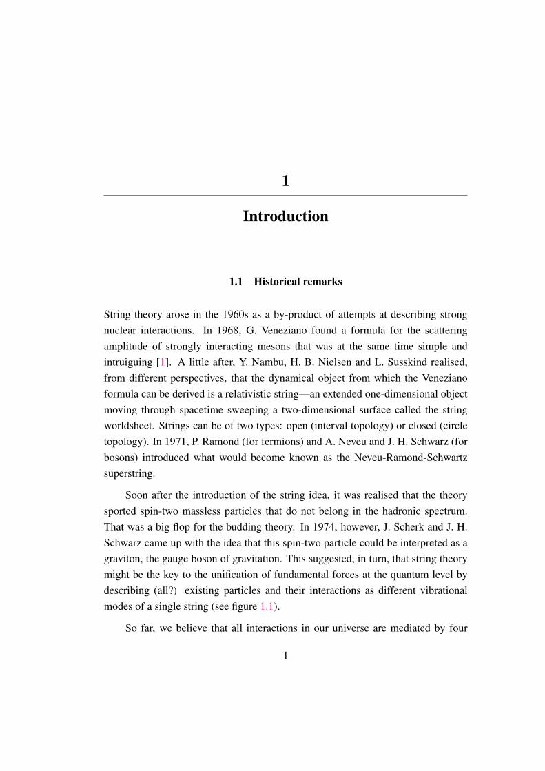
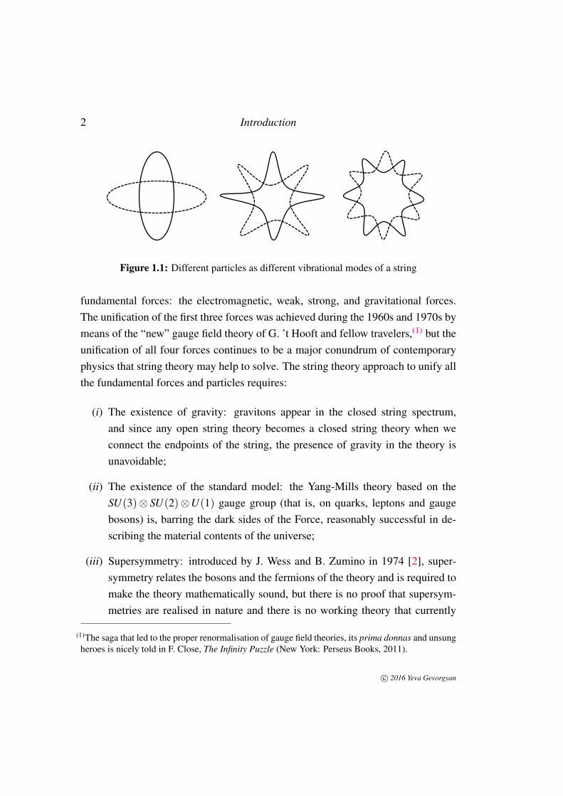
Soon after the introduction of the string idea, it was realised that the theorysported spin-two massless particles that do not belong in the hadronic spectrum.That was a big flop for the budding theory. In 1974, however, J. Scherk and J. H.Schwarz came up with the idea that this spin-two particle could be interpreted as agraviton, the gauge boson of gravitation. This suggested, in turn, that string theorymight be the key to the unification of fundamental forces at the quantum level bydescribing (all?) existing particles and their interactions as different vibrationalmodes of a single string (see figure 1.1).
So far, we believe that all interactions in our universe are mediated by four
1
2 Introduction
Figure 1.1: Different particles as different vibrational modes of a string
fundamental forces: the electromagnetic, weak, strong, and gravitational forces.The unification of the first three forces was achieved during the 1960s and 1970s bymeans of the “new” gauge field theory of G. ’t Hooft and fellow travelers,(1) but theunification of all four forces continues to be a major conundrum of contemporaryphysics that string theory may help to solve. The string theory approach to unify allthe fundamental forces and particles requires:
(i) The existence of gravity: gravitons appear in the closed string spectrum,and since any open string theory becomes a closed string theory when weconnect the endpoints of the string, the presence of gravity in the theory isunavoidable;
(ii) The existence of the standard model: the Yang-Mills theory based on theSU(3)⊗ SU(2)⊗U(1) gauge group (that is, on quarks, leptons and gaugebosons) is, barring the dark sides of the Force, reasonably successful in de-scribing the material contents of the universe;
(iii) Supersymmetry: introduced by J. Wess and B. Zumino in 1974 [2], super-symmetry relates the bosons and the fermions of the theory and is required tomake the theory mathematically sound, but there is no proof that supersym-metries are realised in nature and there is no working theory that currently
(1)The saga that led to the proper renormalisation of gauge field theories, its prima donnas and unsungheroes is nicely told in F. Close, The Infinity Puzzle (New York: Perseus Books, 2011).
c© 2016 Yeva Gevorgyan
1.1 Historical remarks 3
requires supersymmetry. There is, however, some hope that one day super-symmetry will show up in new phenomena or that we will need supersymme-try on the theoretical side of some problem;
(iv) Existence of extra dimensions: modern string theory predicts that spacetimemust be 10 or 11-dimensional. Another possibility is provided by the bosonicstring theory in 26 dimensions (critical dimension), but in this case the massof the string squared is found to be negative, making the theory unstable;
(v) Compactification of extra dimentions: we can argue, by dimensional analysis,that the size of the string should be of the order of the Plank length
`P =
√hGc3 = 1.6×10⁻³³ cm,
and, accordingly, that its mass should be of the order of the Plank mass
mP =
√hcG
= 1.2×10¹⁹ GeV/c2.
To detect an object of size `P we need energies like mP, and this is why wecannot possibly hope to observe strings in the wild and, most likely, will neverdo it by any direct method. The theory must then provide means to compactifysome extra tiny dimensions into non-observable corners of the spacetime atlower energies.
String theory was almost abandoned after the discovery that gravitational andgauge anomalies plagued the theory. But in 1984, M. Green and J. H. Schwarzshowed that the open superstring is free of anomalies if the gauge group of thetheory is SO(32) [3]. Ten-dimensional supersymmetric Einstein-Yang-Mills fieldtheory is also anomaly free with the E8×E8 gauge group. This group appeared firstin string theory and later was used to formulate the theory of the heterotic string,a hybrid beast part 26-dimensional bosonic string, part 10-dimensional superstringadvanced by D. Gross, J. Harvey, E. Martinec and R. Rohm in 1985 [4].
c© 2016 Yeva Gevorgyan
4 Introduction
By 1994, the string theory programme counted on five different 10-dimensionalcontenders: the type I theory, two heterotic theories (the SO(32) and the E8×E8
theories), and the types IIA and IIB theories. In 1995, E. Witten proposed a possible“unification” of these theories by means of dualities [5]. The new formulated theorylives in 11 dimensions, from which the former five 10-dimensional theories arerecovered as different limits. The theory is called M-theory, although nobody issure about what the “M” in its name stands for.(2). Later J. Polchinski found that thetheories can bear additional degrees of freedom for the strings, effectively turningthem into D-branes; strings are then just 1-branes.
The most significant recent development in the string theory programme camein 1998, when J. Maldacena formulated the AdS/CFT gauge-gravity duality con-jecture [6, 7]. According to this conjecture, there is an holographic duality relatingtwo theories with different dimensionalities: in the one side a 4-dimensional gaugetheory and in the other side a 5-dimensional anti-de Sitter spacetime. Many haveargued that the AdS/CFT correspondence is the most important development in allof theoretical physics since the establishment of general relativity in the beginningof the XX century.
Any further account of the string programme would require much deeper anddetailed considerations that are way beyond our current degree of comprehensionor interest, so we stop our historical perspective here and refer the reader to theliterature for additional enlightening.(3)
(2)E. Witten refuses to tell what he had in mind when he coined the moniker; maybe the “M” is justan inverted “W,” maybe it stands for “mother,” maybe for “master”—maybe for “moniker!”
(3)At a nontechnical level, the books by B. Greene, The Elegant Universe: Superstrings, HiddenDimensions, and the Quest for the Ultimate Theory (New York: W. W. Norton, 2003) and L. Randall,Warped Passages: Unraveling the Mysteries of the Universe’s Hidden Dimensions (New York:Harper, 2006) provide good panoramas of the post “second revolution” status of string theory.
c© 2016 Yeva Gevorgyan
1.2 This dissertation 5
1.2 This dissertation
This dissertation summarises our modest attempt at understanding the basic ideasthat build up the string theory approach to high-energy physics. Basically, we studyhow the bosonic string can be described and quantised in the most elementary terms.
The work is organised as follows. In Chapter 2, after briefly reviewing thedynamics of relativistic point particles, we introduce the Nambu-Goto action forthe classical string and investigate its symmetries and the ensuing equations ofmotion. In the same chapter we also introduce the string sigma model action,analyse its symmetries, and introduce and solve the respective equations of motion.In Chapter 3 we present the covariant quantisation of the closed string, introducethe Virasoro algebra and the constraints for the closed string. Next comes the light-cone quantisation of the bosonic string. At the end of Chapter 3 we derive thespectrum of the closed bosonic string. Chapter 4 is reserved for an introductionto the conformal field theory (CFT) aspects and the Virasoro algebra implied inthe study of the bosonic string. There we discuss the stress-energy tensor, Noethercurrents, operator product expansions, the Ward identities and the primary operatorsin the context of CFT. The Faddeev-Popov method for finding the Jacobian for thepath integral of the Polyakov action is described in Chapter 5, where some aspectsof the ghost’s CFT and Virasoro algebra are also described and where we also finallyintroduce the BRST operators and discuss BRST symmetry for the bosonic string.Chapter 6 summarises our presentation, elaborate on further possible studies andconclude the work. A couple of technical derivations were relegated to appendices,four in total.
c© 2016 Yeva Gevorgyan

2
Relativistic string action
In this chapter we discuss the motion of a relativistic free point particle. We intro-duce the action and give some general aspects of its quantisation. We then introducethe Nambu-Goto and the Polyakov actions of the string. We consider for bothactions basic aspects like symmetries and equations of motion. For the Polyakovaction, that we will quantise later, we provide a more detailed review.
General references for the material on this chapter are the introductory bookson string theory by Zwiebach [8] and by Becker, Becker and Schwartz [9], as well asthe more advanced presentation by Green, Schwartz, and Witten [10]. The lecturenotes by Tong [11] and Arutyunov [12] are also helpful.
2.1 Point particle action
In this section we will consider the motion of a free relativistic point particle inD-dimensional Minkowski spacetime. Its motion can be described by means of itsaction functional. The classical point particle moves along geodesics, which meansthat the action has to be proportional to the invariant length of the trajectory of theparticle,
S0 =−α
∫ds, (2.1)
where α is a constant and s is the metric element. In a frame with fixed coordinatesX µ = (t,~x) the action can be written as
S0 =−α
∫ √dt2−d~x2.
7
8 Relativistic string action
t
x
tf
xf0
0
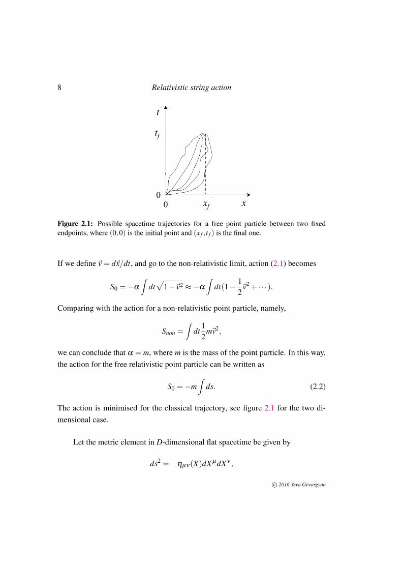
Figure 2.1: Possible spacetime trajectories for a free point particle between two fixedendpoints, where (0,0) is the initial point and (x f , t f ) is the final one.
If we define~v = d~x/dt, and go to the non-relativistic limit, action (2.1) becomes
S0 =−α
∫dt√
1−~v2 ≈−α
∫dt(1− 1
2~v2 + · · ·).
Comparing with the action for a non-relativistic point particle, namely,
Snon =∫
dt12
m~v2,
we can conclude that α = m, where m is the mass of the point particle. In this way,the action for the free relativistic point particle can be written as
S0 =−m∫
ds. (2.2)
The action is minimised for the classical trajectory, see figure 2.1 for the two di-mensional case.
Let the metric element in D-dimensional flat spacetime be given by
ds2 =−ηµν(X)dX µdXν ,
c© 2016 Yeva Gevorgyan
2.1 Point particle action 9
where X µ and Xν are the coordinates of the D-dimensional spacetime and ηµν
describes the geometry of the problem, with µ,ν = 0, 1, · · · , D−1. With the usualMinkowski signature (−+ · · ·+), we can write the action of the point particle as
S0 =−m∫ √
−ηµν(X)X µ Xν dτ, (2.3)
where we introduced the parameter τ , which gives the position along the world lineof the particle, and the dot denotes derivative with respect to τ . The world line of aparticle is the path of the particle in spacetime, tracing the history of its location inspace at each instant in time.
Looking at the action (2.3) we could think that our physical system has Ddegrees of freedom, because the time direction is one of our dinamical variables,but this is not true. This is due to the τ reparameterisation invariance of the action,which is a gauge symmetry of the system. When we go to a new parametrisation ofthe world line τ → τ = τ(τ), we have
dτ = dτ
∣∣∣∣dτ
dτ
∣∣∣∣ anddX µ
dτ=
dX µ
dτ
dτ
dτ. (2.4)
Under these transformations the action becomes
S0 =−m∫ ∣∣∣∣dτ
dτ
∣∣∣∣dτ
√−ηµν
dX µ
dτ
dτ
dτ
dXν
dτ
dτ
dτ=−m
∫ √−ηµν(X)X µ Xν dτ, (2.5)
which has the same form as action (2.3). The consequence of this is that we actuallyhave only D−1 degrees of freedom. For example, we find all X µ in terms of τ , andthen by using the reparameterisation invariance set
τ = X0(τ)≡ t.
If we plug this choice into action (2.3) we find
S0 =−m∫
dt√
1−~v2, (2.6)
c© 2016 Yeva Gevorgyan
10 Relativistic string action
which has D− 1 derees of freedom. So one of initial degrees of freedom is fake.We can check this also by computing the momenta
pµ =∂L
∂ X µ=
mXνηµν√−ησρ(X)Xσ Xρ
, (2.7)
Where L is the Lagrangian of the system. These momenta are not independent,since they satisfy the mass-shell constraint
m2 + pµ pµ = 0 (2.8)
for a relativistic particle with mass m. The mass-shell constraint tells us that in aMinkowski spacetime particles are always moving, at least in the time direction,with (p0)2 > m2.
2.1.1 About quantisation
Action (2.3) contains a square root, which makes it difficult to quantise by the pathintegral approach. Also, it cannot describe the motion of massless particles. Toavoid these problems, we introduce another action for the relativistic point particlewhich is equivalent to the former one at the classical level. First we introduce a newfield e(τ) (as in [9]) on the world line and write the new action as
S0 =12
∫dτ(e−1X2−m2e), (2.9)
where X2 = ηµν X µ Xν . This action should again be invariant under τ reparametri-sation. We can see this by considering an infinitesimal change of reparameterisation
τ → τ′ = f (τ) = τ− ε(τ),
c© 2016 Yeva Gevorgyan
2.1 Point particle action 11
where ε(τ) 1 is an infinitesimal parameter. Under this reparameterisation thefields X µ transform as a world line scalars, X µ ′(τ ′) = X µ(τ), so that to first order
δX µ = X µ ′(τ)−X µ(τ) = ε(τ)X µ .
The additional field e(τ) should transform as e′(τ ′)dτ ′ = e(τ)dτ . Infinitesimally,
δe = e′(τ)− e(τ) =d
dτ(εe).
Now we vary the action (2.9) to obtain
δ S0 =12
∫dτ
(2X µδ Xµ
e−
X µ Xµ
e2 δe−m2δe)
(2.10)
Using the expressions for δe and δX µ we find that
δ S0 =12
∫dτ
(2X µ
e(εXµ + εXµ)−
X µ Xµ
e2 (εe+ ε e)−m2 d(εe)dτ
)(2.11)
The last term drops out because it is a total derivative. The rest can be written as
δ S0 =12
∫dτ
ddτ
(ε
eX µ Xµ
), (2.12)
which is also a total derivative. So δ S0 = 0 and S0 is invariant under τ reparameter-isations. The equation of motion for e(τ) follows from the principle of least action
δ S0
δe=−1
2(e−2X µ Xµ +m2) = 0, (2.13)
orX µ Xµ + e2m2 = 0. (2.14)
It may seem that our new action has one additional degree of freedom compared tothe initial action, but this is not true, since e(τ) is completely fixed by its equationof motion. If we find e(τ) from (2.14) and plug it back into (2.9) we recover the
c© 2016 Yeva Gevorgyan
12 Relativistic string action
action functional (2.3). Now we notice that S0 can be rewritten as
S0 =12
∫ (ηµν(X)dX µ dXν
e(τ)dτ−m2e(τ)
)dτ. (2.15)
Since e(τ) always appears multiplied by dτ in the above expression and the actionis τ-reparameterisation invariant, we can absorb e(τ) into dτ , which is tantamountto choosing e(τ) = 1 from the beginning, for this choice is largely irrelevant for thephysics of the problem. Reparametrisation invariance thus allows us to choose agauge with e(τ) = 1, which gives
X µ Xµ +m2 = 0. (2.16)
Identifying X µ = pµ , the momentum conjugated to X µ , we see that this equation isin fact just the mass-shell constraint p2 +m2 = 0. The variation of S0 with respectto X µ gives a second set of equations of motion,
δ S0
δX µ=− d
dτ(ηµν Xν)+
12
∂µηρλ Xρ Xλ
=−(∂ρηµν)Xρ Xν −ηµν Xν +12
∂µηρλ Xρ Xλ .
(2.17)
We can bring this equation to the form
X µ +Γµ
ρλXρ Xλ = 0, (2.18)
whereΓ
µ
ρλ=
12
ηµν(∂ρηλν +∂λ ηρν −∂νηρλ
)(2.19)
is the Levi-Civita connection. Equation (2.18) is the equation for the geodesicson the spacetime described by gµν , or, equivalently, Newton’s equation for a freeparticle in curved spacetime. For flat spacetime, Γ
µ
ρλvanishes and we recover the
usual equation of motion for a pointlike free particle.
c© 2016 Yeva Gevorgyan
2.2 The Nambu-Goto action 13
2.2 The Nambu-Goto action
Another important action is the Nambu-Goto string action, which describes the rela-tivistic theory but, as we will see later, is not suited for the path integral quantisationof string theory.
Consider the motion of a relativistic string propagating in a D-dimensionalMinkowski spacetime. While moving, the string draws a two dimensional surfacecalled its worldsheet. We parametrise the worldsheet by the time-like coordinateσ0 = τ and the space-like coordinate σ1 = σ . Depending on σ , the string will beclosed (periodic σ ) or open (σ covering a finite interval). The action for the motionof the relativistic string is then taken to be proportional to the proper area of itsworldsheet and is given by
SNG =−T∫
d2σ
√(X ·X ′)2− X2X ′2, (2.20)
where T is the tension of the string (with dimension of mass per length) and
X µ =∂X µ
∂τ, X ′µ =
∂X µ
∂σ. (2.21)
SNG in (2.20) is called the Nambu-Goto action of a relativistic string. From thisaction we can see that the classical string motion minimises the worldsheet area.
Now we define an induced metric γαβ on the worldsheet as
γαβ = ηµν
∂X µ
∂σα
∂Xν
∂σβ. (2.22)
Accordingly, the Nambu-Goto action becomes
SNG =−T∫
d2σ√−γ (2.23)
where γ = detγαβ . Written in this form, SNG is manifestly reparameterisationinvariant.
c© 2016 Yeva Gevorgyan
14 Relativistic string action
2.2.1 Symmetries
The Nambu-Goto action has two types of global symmetries:
Poincaré invariance of the spacetime: X µ → Λµ
ν Xν + cµ , where Λ is a Lorentztransformation satisfying Λ
µ
ν ηνρΛσρ = ηµσ and cµ is a constant translation. The
symmetry is global from the perspective of the worldsheet, this means that Λµ
ν andcµ are constants and do not depend on worldsheet coordinates σα .
Reparametrisation invariance: Also known as diffeomorphisms, reparametrisa-tions are gauge symmetries on the worldsheet. The transformations
σα → f α(σ) = σ
′α and gαβ (σ) =∂ f λ
∂σα
∂ f ρ
∂σβgλρ(σ
′) (2.24)
keep the action invariant. This type of symmetry implies that the transformationsand their inverses are infinitely differentiable. Sometimes these transformations areused in infinitesimal form. If we change coordinates σα → σ ′α = σα −ηα(σ) forsome small η , the transformations of the fields become
δX µ(σ) = ηα
∂αX µ
δgαβ (σ) = ∇αηβ +∇β ηα ,(2.25)
where the covariant derivative is defined by ∇αηβ = ∂αηβ −Γσ
αβησ with the Levi-
Civita connection given by
Γσ
αβ=
12
gσρ(∂αgβρ +∂β gρα −∂ρgαβ ).
2.2.2 Equations of motion
Let us obtain the equations of motion for the Nambu-Goto action. First we rewritethe action in terms of a Lagrangian density,
SNG =∫
τ f
τi
dτ
∫σ1
0dσ LNG(X µ ,X ′µ), (2.26)
c© 2016 Yeva Gevorgyan
2.2 The Nambu-Goto action 15
whereLNG(X µ ,X ′µ) =−T
√(X ·X ′)2− X2X ′2 . (2.27)
To obtain the equations of motion we calculate the first variation of the action (2.26),
δSNG =∫
τ f
τi
dτ
∫σ1
0dσ
[∂LNG
∂ X µ
∂ (δX µ)
∂τ+
∂LNG
∂X ′µ∂ (δX µ)
∂σ
], (2.28)
and set it to zero. For brevity of notation we introduce the quantities
Πτµ =
∂LNG
∂ X µ=−T
(X ·X ′)X ′µ −X ′2Xµ√(X ·X ′)2− X2X ′2
, (2.29)
Πσµ =
∂LNG
∂X ′µ=−T
(X ·X ′)Xµ − X2X ′µ√(X ·X ′)2− X2X ′2
. (2.30)
Using this notation (2.28) becomes
δSNG =∫
τ f
τi
dτ
∫σ1
0dσ
[∂
∂τ
(δX µ
Πτµ
)+
∂
∂σ
(δX µ
Πσµ
)−δX µ
(∂Πτ
µ
∂τ+
∂Πσµ
∂σ
)].
(2.31)For initial and final moments of time we put δX µ(τ f ,σ) = δX µ(τi,σ) = 0. Thevariation of the action with respect to X µ then becomes
δSNG =∫
τ f
τi
dτ
[δX µ
Πσµ
]σ1
0−∫
τ f
τi
dτ
∫σ1
0dσδX µ
(∂Πτ
µ
∂τ+
∂Πσµ
∂σ
). (2.32)
Since the second term in the right hand side of (2.32) should vanish for all variationsδX µ of the motion, we obtain
∂Πτµ
∂τ+
∂Πσµ
∂σ= 0. (2.33)
c© 2016 Yeva Gevorgyan
16 Relativistic string action
This is an equation of motion for both open and closed relativistic strings. The firstterm in the right hand side can be written explicitly as∫
τ f
τi
dτ[δX0(τ,σ1)Π
σ0 (τ,σ1)−δX0(τ,0)Πσ
0 (τ,0)
+δX1(τ,σ1)Πσ1 (τ,σ1)−δX1(τ,0)Πσ
1 (τ,0)...
+δXD−1(τ,σ1)ΠσD−1(τ,σ1)−δXD−1(τ,0)Πσ
D−1(τ,0)].
(2.34)
We see that we need a total of 2D boundary conditions, one for each term in (2.34).For the open string we can impose two types of boundary conditions:
Dirichlet boundary condition: In this case the spatial coordinates of the endpointare fixed, say, at σ ′, and we impose, for every µ 6= 0, that
∂X µ
∂τ(τ,σ ′) = 0. (2.35)
Since time varies as τ varies,∂X0
∂τ6= 0, Dirichlet boundary conditions are applicable
only to spatial coordinates.
Neumann boundary condition: In this case we impose
Πσµ (τ,σ
′) = 0 (2.36)
for every µ = 0,1, . . . ,D−1. This boundary condition is also called “free endpointboundary condition.”
Any one of these two boundary conditions make (2.34) vanish.
For the closed string we pick σ1 to be an integer multiple of π , in which casethe first term in the equation (2.32) vanishes identically.
We can write the equations of motion (2.33) in a leaner fashion. From the
c© 2016 Yeva Gevorgyan
2.3 The string sigma model action 17
definition of γαβ and Jacobi’s formula for differentiating a determinant,
δ√−γ =− 1
2√−γ
δγ =−12√−γ γαβ δγ
αβ =12√−γ γ
αβδγαβ , (2.37)
variation of the action (2.23) provides the equations
∂α
(√−γ γ
αβ∂β X µ
)= 0. (2.38)
Even though the equations of motion look better in this notation, they are still thesame nasty equations!
2.3 The string sigma model action
The Nambu-Goto action contains a square-root that makes it troublesome to quan-tise by the path integral approach. There is, however, another action which is moreconvenient to quantise and that recovers the Nambu-Goto action in the classicallimit. We can get rid of the square root in SNG by introducing a new field gαβ to theaction and by rewriting it as
S =−12
T∫
d2σ√−ggαβ
∂αX µ∂β Xν
ηµν , (2.39)
where g = detgαβ , and gαβ = (gαβ )−1. This action is called the Polyakov or the
sigma model action. The new field gαβ is a dynamical metric on the worldsheet.From the point of view of the worldsheet, the sigma model action describes a bunchof scalar fields X µ coupled to two-dimensional gravity gαβ .
The Polyakov action gives rise to the same equations of motion (2.38) as theNambu-Goto action but with gαβ in the place of γαβ ,
∂α
(√−ggαβ
∂β X µ)= 0. (2.40)
However, gαβ is now an independent variable which should be fixed by its ownequations of motion. To determine the equivalence of the equations of motion we
c© 2016 Yeva Gevorgyan
18 Relativistic string action
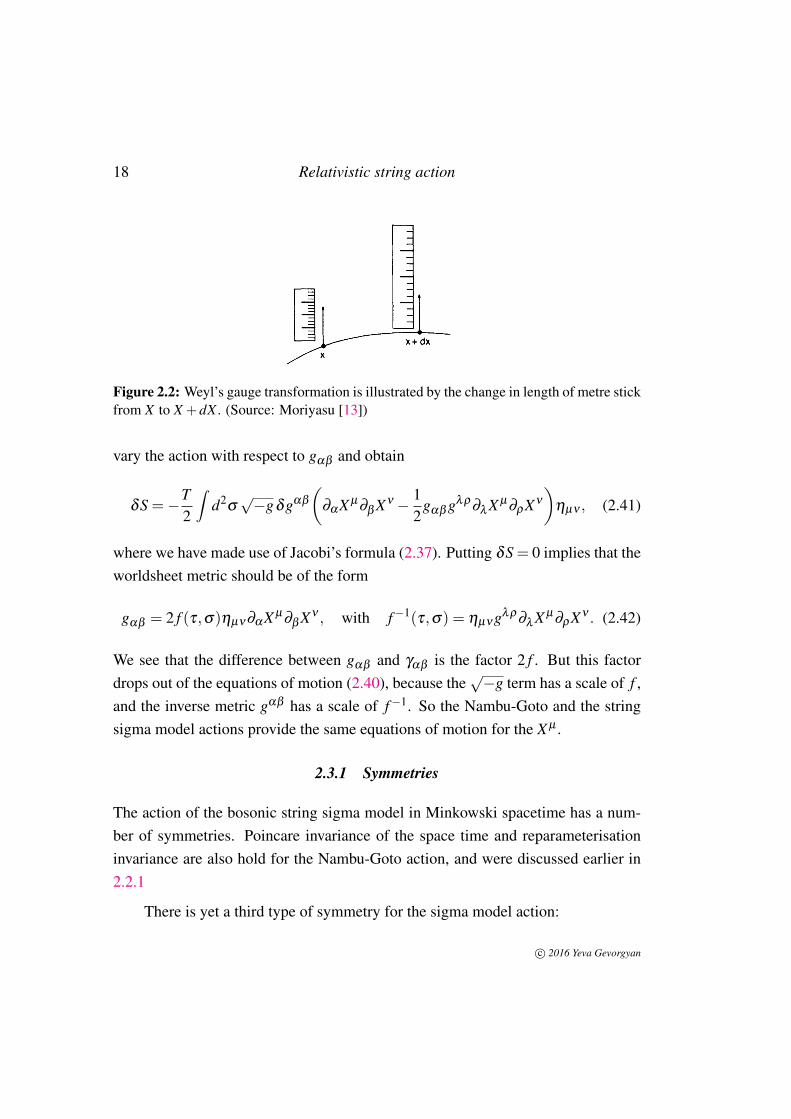
Figure 2.2: Weyl’s gauge transformation is illustrated by the change in length of metre stickfrom X to X +dX . (Source: Moriyasu [13])
vary the action with respect to gαβ and obtain
δS =−T2
∫d2
σ√−gδgαβ
(∂αX µ
∂β Xν − 12
gαβ gλρ∂λ X µ
∂ρXν
)ηµν , (2.41)
where we have made use of Jacobi’s formula (2.37). Putting δS = 0 implies that theworldsheet metric should be of the form
gαβ = 2 f (τ,σ)ηµν∂αX µ∂β Xν , with f−1(τ,σ) = ηµνgλρ
∂λ X µ∂ρXν . (2.42)
We see that the difference between gαβ and γαβ is the factor 2 f . But this factordrops out of the equations of motion (2.40), because the
√−g term has a scale of f ,
and the inverse metric gαβ has a scale of f−1. So the Nambu-Goto and the stringsigma model actions provide the same equations of motion for the X µ .
2.3.1 Symmetries
The action of the bosonic string sigma model in Minkowski spacetime has a num-ber of symmetries. Poincare invariance of the space time and reparameterisationinvariance are also hold for the Nambu-Goto action, and were discussed earlier in2.2.1
There is yet a third type of symmetry for the sigma model action:
c© 2016 Yeva Gevorgyan
2.3 The string sigma model action 19
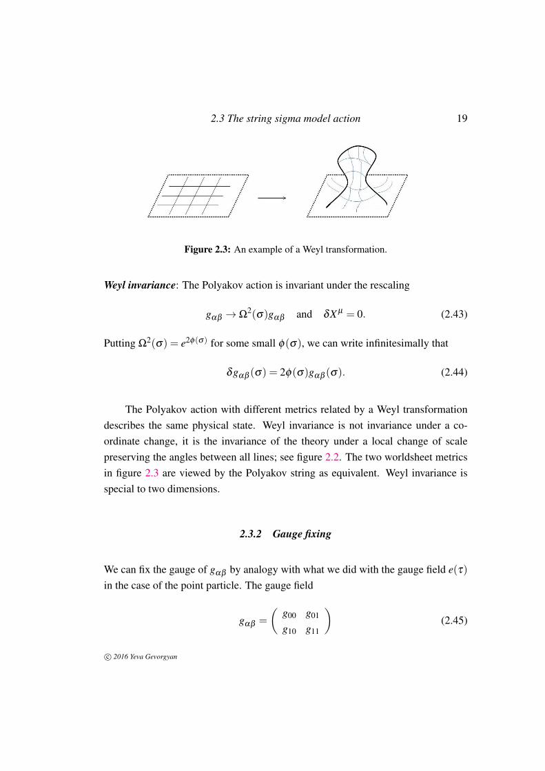
Figure 2.3: An example of a Weyl transformation.
Weyl invariance: The Polyakov action is invariant under the rescaling
gαβ →Ω2(σ)gαβ and δX µ = 0. (2.43)
Putting Ω2(σ) = e2φ(σ) for some small φ(σ), we can write infinitesimally that
δgαβ (σ) = 2φ(σ)gαβ (σ). (2.44)
The Polyakov action with different metrics related by a Weyl transformationdescribes the same physical state. Weyl invariance is not invariance under a co-ordinate change, it is the invariance of the theory under a local change of scalepreserving the angles between all lines; see figure 2.2. The two worldsheet metricsin figure 2.3 are viewed by the Polyakov string as equivalent. Weyl invariance isspecial to two dimensions.
2.3.2 Gauge fixing
We can fix the gauge of gαβ by analogy with what we did with the gauge field e(τ)in the case of the point particle. The gauge field
gαβ =
(g00 g01
g10 g11
)(2.45)
c© 2016 Yeva Gevorgyan
20 Relativistic string action
has three independent components, since g10 = g01. Using the symmetries of themodel we can fix gαβ completely. The choice of a conformal gauge fixes twocomponents by the reparametrisation invariance. Reparameterisation invariance isused to choose coordinates such that locally gαβ = Ω2(σ ,τ)ηαβ with ηαβ the twodimensional Minkowski metric defined by ds2 = −dτ2 + dσ2. Let us show thatthis can be always done. For any 2-dimensional metric gαβ , we consider two nullvectors at each point. Like this we get two vector fields and their integral curves,which we label by σ+ and σ−. Then ds2 = −Ω2dσ+dσ− and g++ = g−− = 0since the curves are null. Now let
σ± = τ±σ ,
from which ds2 = Ω2(−dτ2+dσ2). So we really always can make a choice gαβ =
Ω2(σ ,τ)ηαβ . A choice of coordinate system in which the 2-dimensional metric isconformally flat, i.e. in which
ds2 = Ω2(−dτ
2 +dσ2) =−ω
2dσ+dσ
−, (2.46)
is called a conformal gauge. σ± are called light-cone or conformal coordinates.And now we can use the Weyl rescaling to fix the remaining component,
Ω2(σ ,τ)ηαβ = ηαβ .
As a result the gauge field can be chosen as
gαβ = ηαβ =
(−1 0
0 1
), (2.47)
where ηαβ is a flat worldsheet metric. This choice is possible only if there are notopological obstructions, and if it is allowed the action becomes
S =T2
∫d2
σ ∂αX∂αX . (2.48)
c© 2016 Yeva Gevorgyan
2.3 The string sigma model action 21
For a flat Minkowski spacetime we could have two more renormalisable and Poincaréinvariant terms in the action, namely,
λ1
∫d2
σ√−g and λ2
∫d2
σ√−gR(2)(g). (2.49)
The first term is a cosmological constant term in the worldsheet that is not allowedby the equations of motion.(1) The second term, due to the scalar curvature R(2)(g)of the worldsheet geometry, is allowed but will not be discussed here.
2.3.3 Equations of motion
When gαβ = ηαβ , the Polyakov action becomes the theory of D free scalar fieldswith action (2.48). In this case we can rewrite the equations of motion as
∂α∂αX µ = 0. (2.50)
These equations of motion are not really equal to the initial ones. We must ensurethat the equation of motion for gαβ is also satisfied. The variation of the action with
(1)When we add a cosmological constant term to the string sigma model action (2.39), the firstvariation of S′ = S+λ1
∫d2σ√−g gives, using (2.41) and Jacobi’s formula (2.37),
δS′ =−T2
∫d2
σ δgαβ
(√−g∂α X µ
∂β Xν − 12√−ggαβ gρσ
∂ρ X µ∂σ Xν
)ηµν −
12
λ1√−ggαβ δgαβ ,
and the equation of motion for the worldsheet metric becomes
2√−g
δSσ
δgαβ=−T
[(∂α X µ
∂β Xν − 12
gαβ gρσ∂ρ X µ
∂σ Xν)ηµν
]−λ1gαβ = 0.
Multiplying the last equation by gαβ furnishes
gαβ gαβλ1 = T
(12
gαβ gαβ −1)
gαβ∂ρ X µ
∂σ Xνηµν = 0,
because gαβ gαβ = 2. Consistency of the equations of motion thus requires that λ1 = 0.
c© 2016 Yeva Gevorgyan
22 Relativistic string action
respect to the metric gives rise to the stress-energy tensor
Tαβ =− 2T
1√−g
∂S∂gαβ
. (2.51)
If we set gαβ =ηαβ in equations (2.41) and (2.51), the stress-energy tensor becomes
Tαβ = ∂αX µ∂β Xµ −
12
ηαβ ηρσ
∂ρX µ∂σ Xµ . (2.52)
The equation of motion for gαβ is just Tαβ = 0. Explicitly,
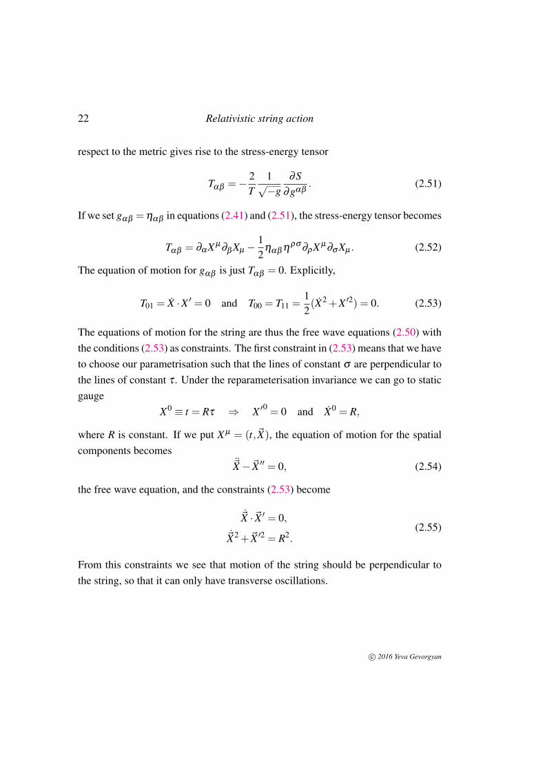
T01 = X ·X ′ = 0 and T00 = T11 =12(X2 +X ′2) = 0. (2.53)
The equations of motion for the string are thus the free wave equations (2.50) withthe conditions (2.53) as constraints. The first constraint in (2.53) means that we haveto choose our parametrisation such that the lines of constant σ are perpendicular tothe lines of constant τ . Under the reparameterisation invariance we can go to staticgauge
X0 ≡ t = Rτ ⇒ X ′0 = 0 and X0 = R,
where R is constant. If we put X µ = (t,~X), the equation of motion for the spatialcomponents becomes
~X−~X ′′ = 0, (2.54)
the free wave equation, and the constraints (2.53) become
~X ·~X ′ = 0,
~X2 +~X ′2 = R2.(2.55)
From this constraints we see that motion of the string should be perpendicular tothe string, so that it can only have transverse oscillations.
c© 2016 Yeva Gevorgyan
2.3 The string sigma model action 23
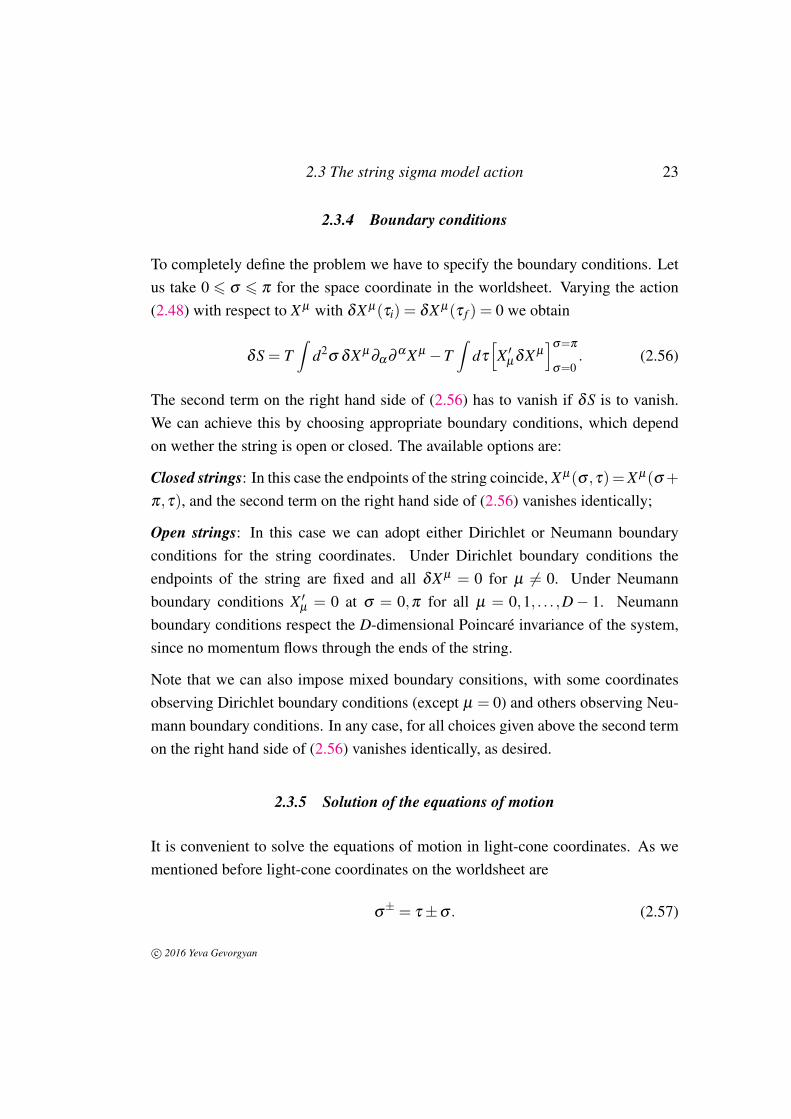
2.3.4 Boundary conditions
To completely define the problem we have to specify the boundary conditions. Letus take 0 6 σ 6 π for the space coordinate in the worldsheet. Varying the action(2.48) with respect to X µ with δX µ(τi) = δX µ(τ f ) = 0 we obtain
δS = T∫
d2σ δX µ
∂α∂αX µ −T
∫dτ
[X ′µδX µ
]σ=π
σ=0. (2.56)
The second term on the right hand side of (2.56) has to vanish if δS is to vanish.We can achieve this by choosing appropriate boundary conditions, which dependon wether the string is open or closed. The available options are:
Closed strings: In this case the endpoints of the string coincide, X µ(σ ,τ)=X µ(σ +
π,τ), and the second term on the right hand side of (2.56) vanishes identically;
Open strings: In this case we can adopt either Dirichlet or Neumann boundaryconditions for the string coordinates. Under Dirichlet boundary conditions theendpoints of the string are fixed and all δX µ = 0 for µ 6= 0. Under Neumannboundary conditions X ′µ = 0 at σ = 0,π for all µ = 0,1, . . . ,D− 1. Neumannboundary conditions respect the D-dimensional Poincaré invariance of the system,since no momentum flows through the ends of the string.
Note that we can also impose mixed boundary consitions, with some coordinatesobserving Dirichlet boundary conditions (except µ = 0) and others observing Neu-mann boundary conditions. In any case, for all choices given above the second termon the right hand side of (2.56) vanishes identically, as desired.
2.3.5 Solution of the equations of motion
It is convenient to solve the equations of motion in light-cone coordinates. As wementioned before light-cone coordinates on the worldsheet are
σ± = τ±σ . (2.57)
c© 2016 Yeva Gevorgyan

24 Relativistic string action
The derivatives and the two-dimensional Lorentz metric in these coordinates aregiven by
∂± =12(∂τ ±∂σ ) and
(η++ η+−
η−+ η−−
)=−1
2
(0 11 0
). (2.58)
The equation of motion for X µ now reads
∂+∂−X µ = 0. (2.59)
Let us consider solutions for this equation in open and closed string cases.
Closed strings: The most general solution for this equation is
X µ(σ ,τ) = X µ
L (σ+)+X µ
R (σ−) (2.60)
for arbitrary functions X µ
L and X µ
R , which we call left and right moving waves forreasons that will be clear in the following. Solution X µ(σ ,τ) must respect theconstraints (2.53) and be periodic,
X µ(σ ,τ) = X µ(σ +π,τ). (2.61)
We then expand each of the terms of the solution (2.60) in Fourier modes,
X µ
L (σ+) =12
xµ +12
α′pµ
σ++ i
√α ′
2 ∑n6=0
1n
αµn e−2inσ+
,
X µ
R (σ−) =12
xµ +12
α′pµ
σ−+ i
√α ′
2 ∑n6=0
1n
αµn e−2inσ−.
(2.62)
The mode expansion is important for quantisation. The following observationsabout the above mode expansions apply:
• X µ
L and X µ
R are not individually π periodic but their sum and difference are;
c© 2016 Yeva Gevorgyan
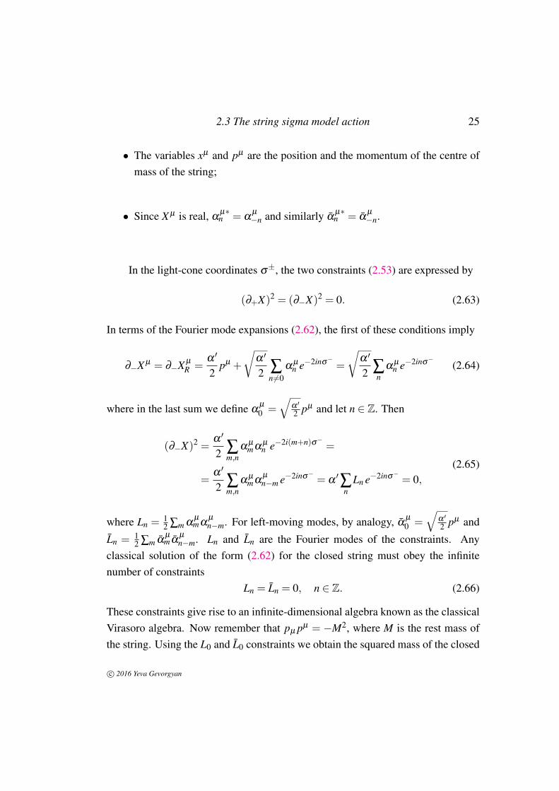
2.3 The string sigma model action 25
• The variables xµ and pµ are the position and the momentum of the centre ofmass of the string;
• Since X µ is real, αµ∗n = α
µ
−n and similarly αµ∗n = α
µ
−n.
In the light-cone coordinates σ±, the two constraints (2.53) are expressed by
(∂+X)2 = (∂−X)2 = 0. (2.63)
In terms of the Fourier mode expansions (2.62), the first of these conditions imply
∂−X µ = ∂−X µ
R =α ′
2pµ +
√α ′
2 ∑n6=0
αµn e−2inσ− =
√α ′
2 ∑n
αµn e−2inσ− (2.64)
where in the last sum we define αµ
0 =√
α ′2 pµ and let n ∈ Z. Then
(∂−X)2 =α ′
2 ∑m,n
αµmα
µn e−2i(m+n)σ− =
=α ′
2 ∑m,n
αµmα
µ
n−m e−2inσ− = α′∑n
Ln e−2inσ− = 0,(2.65)
where Ln =12 ∑m α
µmα
µ
n−m. For left-moving modes, by analogy, αµ
0 =√
α ′2 pµ and
Ln = 12 ∑m α
µm α
µ
n−m. Ln and Ln are the Fourier modes of the constraints. Anyclassical solution of the form (2.62) for the closed string must obey the infinitenumber of constraints
Ln = Ln = 0, n ∈ Z. (2.66)
These constraints give rise to an infinite-dimensional algebra known as the classicalVirasoro algebra. Now remember that pµ pµ = −M2, where M is the rest mass ofthe string. Using the L0 and L0 constraints we obtain the squared mass of the closed
c© 2016 Yeva Gevorgyan
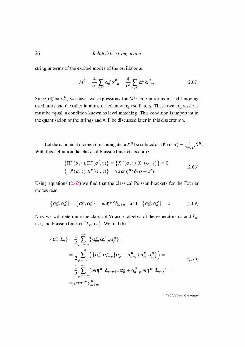
26 Relativistic string action
string in terms of the excited modes of the oscillator as
M2 =4α ′ ∑n>0
αµn α
µ
−n =4α ′ ∑n>0
αµn α
µ
−n. (2.67)
Since αµ
0 = αµ
0 , we have two expressions for M2: one in terms of right-movingoscillators and the other in terms of left-moving oscillators. These two expressionsmust be equal, a condition known as level matching. This condition is important inthe quantisation of the strings and will be discussed later in this dissertation.
Let the canonical momentum conjugate to X µ be defined as Πµ(σ ,τ)=1
2πα ′X µ .
With this definition the classical Poisson brackets becomeΠ
µ(σ ,τ),Πν(σ ′,τ)=
X µ(σ ,τ),Xν(σ ′,τ)= 0,
Πµ(σ ,τ),Xν(σ ′,τ)
= 2πα
′η
µνδ (σ −σ
′).(2.68)
Using equations (2.62) we find that the classical Poisson brackets for the Fouriermodes read
αµm ,α
νn=
αµm , α
νn= imη
µνδm+n and
α
µm , α
νn= 0. (2.69)
Now we will determine the classical Virasoro algebra of the generators Ln and Ln,i. e., the Poisson bracket Lm,Ln. We find that
α
νm,Ln
=
12
+∞
∑p=−∞
α
νm,α
µ
n−pαµp=
=12
+∞
∑p=−∞
(α
νm,α
µ
n−p
αµp +α
µ
n−p
ανm,α
µp)
=
=12
+∞
∑p=−∞
(imη
µνδn−p+mα
µp +α
µ
n−pimηµν
δm+p)=
= imηµν
αµ
m+n,
(2.70)
c© 2016 Yeva Gevorgyan
2.3 The string sigma model action 27
from which follows
Lm,Ln
=
12
+∞
∑p=−∞
α
µ
m−pαµp ,Ln
=
=12
+∞
∑p=−∞
(α
µ
m−p,Ln
αµp +α
µ
m−p
αµp ,Ln
)=
=12
imηµν
+∞
∑p=−∞
(α
νm−p+nα
µp +α
µ
m−pανp+n).
(2.71)
Changing m→ n in the first term and p+n→ q in the second term of the summationon the right-hand side of equation (2.71) provides
Lm,Ln
=
12
inηνµ
+∞
∑p=−∞
αµ
m+n−pανp +
12
imηµν
+∞
∑q=−∞
αµ
m+n−qανq =
= i(m−n)Lm+n,
(2.72)
which is the defining commutation relation for the classical Virasoro algebra.
Open strings: The Fourier mode expansion for the open string reads
X µ
L (σ+) =12
xµ +α′pµ
σ++ i
√α ′
2 ∑n6=0
1n
αµn e−inσ+
,
X µ
R (σ−) =12
xµ +α′pµ
σ−+ i
√α ′
2 ∑n6=0
1n
αµn e−inσ−.
(2.73)
Boundary conditions impose relations on the modes of the open string:
• Neumann boundary conditions ∂σ Xa = 0, at the endpoints require that αan =
αan , which gives
X µ(σ ,τ) = X µ +2α′pµ
τ + i√
2α ′ ∑n6=0
1n
αµn e−inτ cosnσ . (2.74)
For open strings there is only one set of modes αµn . Instead of right and
c© 2016 Yeva Gevorgyan
28 Relativistic string action
left-moving modes we have just standing waves.
• Direchlet boundary conditions, X I = cI , at the end point srequire that xI = cI ,pI = 0 and α I
n =−α In. which gives
X µ(σ ,τ) = cI +√
2α ′ ∑n 6=0
1n
αµn e−inτ sinnσ . (2.75)
For the open string, constraints (2.53) are also like in equation (2.63). The Fouriermode expansion of these conditions imply
2∂±X µ = X µ ±X ′µ =
√α ′
2
∞
∑n=−∞
αµn e−in(τ±σ), (2.76)
where αµ
0 =√
α ′2 pµ , as before. By analogy with the closed string, we find the
Fourier modes of the constraints, just in this case we have only one set of Ln. Soany classical solution of the form (2.74) for the open string must obey the infinitenumber of constraints
Ln = 0, n ∈ Z. (2.77)
For the open string we find, that the squared mass is given by
M2 =1α ′
(p−1
∑i=1
∑n>0
αi−nα
in +
D−1
∑i=p+1
∑n>0
αi−nα
in
). (2.78)
The first sum is over modes parallel to the brane where the end points of the openstring are, the second over perpendicular to the brane.
c© 2016 Yeva Gevorgyan
3
Quantisation of the bosonic string
In this chapter we will consider two ways to quantise the bosonic string:
Covariant quantisation: To quantise the string covariantly we first quantise thesystem and then impose the constraints that arise from the gauge fixing.
Light-cone gauge quantisation: In light-cone gauge quantisation we first solve allthe constraints of the system to determine the space of all classical solutions andthen quantise these solutions.
Our main references for this chapter are the book by Becker, Becker andSchwartz [9] and the lecture notes by Tong [11].
3.1 Covariant quantisation of the closed string
In this section we will quantise D free scalar fields X µ , with dynamics governed bythe action (2.48). For the canonical quantisation we first change Poisson bracketsby commutators
, −→ 1i[ , ]. (3.1)
We define momentum conjugated with X µ as Πµ =1
2πα ′X µ , where µ = 0,1, . . . ,D−
1, quantum mechanical operators obey the following commutation relations
[X µ(σ ,τ),Πν(σ′,τ)] = iδ (σ −σ
′)δµ
ν ,
[X µ(σ ,τ),Xν(σ ′,τ)] = [Πµ(σ ,τ),Πν(σ′,τ)] = 0.
(3.2)
29
30 Quantisation of the bosonic string
These commutation relations can be used to find the commutation relations for theFourier modes xµ , pµ ,α
µn and α
µn . Using (2.62) we find for the closed string
[xµ , pν ] = iδ µ
ν , (3.3)
which is the expected commutation relation for the operators of the center of massof the string. The remaining commutation relations are
[αµm , α
νn ] = 0 and [αµ
n ,ανm] = [αµ
n , ανm] = nη
µνδn+m,0. (3.4)
We see that αµn and α
µn behave like creation and annihilation operators for a set of
harmonic oscillators. Using the rescaling
aµn =
1√n
αµn , for n > 0 (3.5)
and hermicity
aµ†n =
1√n
αµ
−n, for n > 0, (3.6)
we find that
[aµm,a
ν†n ] = η
µνδm,n
[aµm, a
ν†n ] = η
µνδm,n,
(3.7)
which coincide with the standard commutation relations for two infinite sets ofindependent quantum harmonic oscillators. For every integer n we introduce anumber operator
Nn = αµn α−n,µ . (3.8)
Using equations (3.4) and (3.8) we find for every n > 0
[Nn,αn] =−nαn,
[Nn,α−n] = nα−n.(3.9)
c© 2016 Yeva Gevorgyan
3.1 Covariant quantisation of the closed string 31
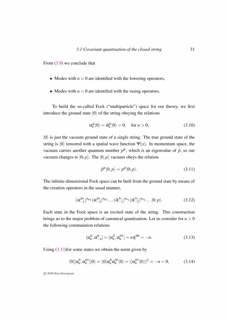
From (3.9) we conclude that
• Modes with n > 0 are identified with the lowering operators,
• Modes with n < 0 are identified with the rasing operators.
To build the so-called Fock (“multiparticle”) space for our theory, we firstintroduce the ground state |0〉 of the string obeying the relations
αµn |0〉= α
µn |0〉= 0, for n > 0; (3.10)
|0〉 is just the vacuum ground state of a single string. The true ground state of thestring is |0〉 tensored with a spatial wave function Ψ(x). In momentum space, thevacuum carries another quantum number pµ , which is an eigenvalue of p, so ourvacuum changes to |0; p〉. The |0, p〉 vacuum obeys the relation
pµ |0, p〉= pµ |0; p〉. (3.11)
The infinite-dimensional Fock space can be built from the ground state by means ofthe creation operators in the usual manner,
(αµ1−1)
nµ1 (αµ2−2)
nµ2 . . .(αν1−1)
nν1 (αν2−2)
nν2 . . . |0; p〉. (3.12)
Each state in the Fock space is an excited state of the string. This constructionbrings us to the major problem of canonical quantisation. Let us consider for n > 0the following commutation relations
[α0n ,α
0−n] = [α0
n ,α0†n ] = nη
00 =−n. (3.13)
Using (3.13)for some states we obtain the norm given by
〈0|[α0n ,α
0†n ]|0〉= 〈0|α0
n α0†n |0〉= ||α0†
n |0〉||2 =−n < 0, (3.14)
c© 2016 Yeva Gevorgyan
32 Quantisation of the bosonic string
that is, we get states with negative norm in the Hilbert space. This states arecalled ghosts and do not allow the probabilistic interpretation of the correspondingquantum-mechanical system. We got ghosts because we ignored the so calledVirasoro constraints, which we will discuss later in this chapter. To make sense ofthe theory, we have to make sure that ghosts do not appear in any physical process.
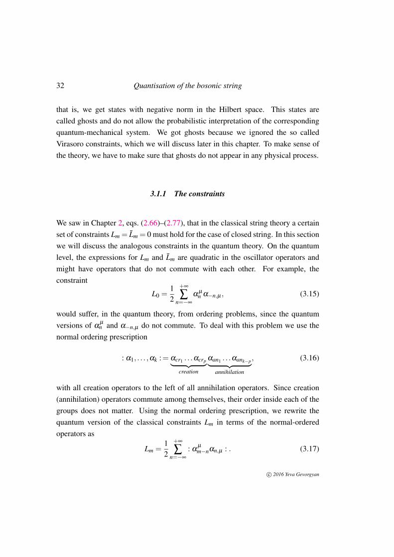
3.1.1 The constraints
We saw in Chapter 2, eqs. (2.66)–(2.77), that in the classical string theory a certainset of constraints Lm = Lm = 0 must hold for the case of closed string. In this sectionwe will discuss the analogous constraints in the quantum theory. On the quantumlevel, the expressions for Lm and Lm are quadratic in the oscillator operators andmight have operators that do not commute with each other. For example, theconstraint
L0 =12
+∞
∑n=−∞
αµn α−n,µ , (3.15)
would suffer, in the quantum theory, from ordering problems, since the quantumversions of α
µn and α−n,µ do not commute. To deal with this problem we use the
normal ordering prescription
: α1, . . . ,αk := αcr1 . . .αcrp︸ ︷︷ ︸creation
αan1 . . .αank−p︸ ︷︷ ︸annihilation
, (3.16)
with all creation operators to the left of all annihilation operators. Since creation(annihilation) operators commute among themselves, their order inside each of thegroups does not matter. Using the normal ordering prescription, we rewrite thequantum version of the classical constraints Lm in terms of the normal-orderedoperators as
Lm =12
+∞
∑n=−∞
: αµ
m−nαn,µ : . (3.17)
c© 2016 Yeva Gevorgyan
3.1 Covariant quantisation of the closed string 33
In particular, the L0 constraint becomes
L0 =12
α20 +
+∞
∑n=1
αµ
−nαn,µ −a, (3.18)
where a is a normal ordering constant.
Since the zero-modes are given in terms of pµ , we also need a prescription forthe normal-ordering of momentum operators, which reads
: pµxν := xν pµ , (3.19)
The zero state |0; p〉 satisfies pµ |0; p〉 = pµ |0; p〉 and can be considered the usual
quantum mechanical eigenstate of the momentum operator pµ = −i∂
∂xµ. In mo-
mentum representation, the zero state is then given by a plane wave
|0; p〉= eipµ xµ |0;0〉. (3.20)
Plane waves are not square-integrable but form the basis of a generalised Hilbertspace if normalised as 〈0; p|0; p′〉= δ (p− p′).
3.1.2 The Virasoro algebra
Classical case
As we saw in the classical theory, the Virasoro generators Lm satisfy the algebra
Lm,Ln= i(m−n)Lm+n. (3.21)
The Virasoro constraints appear because the gauge choice
gαβ = ηαβ =
(−1 0
0 1
)(3.22)
does not fully fix the reparametrisation gauge symmetry. If ξ α is an infinitesimal
c© 2016 Yeva Gevorgyan
34 Quantisation of the bosonic string
parameter of the reparametrisation and Λ is an infinitesimal parameter of the Weylrescaling, then residual reparametrisation symmetries, which satisfy
∂α
ξβ +∂
βξ
α = Ληαβ , (3.23)
remain in the theory. These reparameterisations are also Weyl rescalings, discussedearlier in section 2.2.1. If we put
ξ± = ξ
0±ξ1 and σ
± = σ0±σ
1,
we find thatξ+ = ξ
+(σ+) and ξ− = ξ
−(σ−)
are solutions of equation (3.23). The infinitesimal generators for the transformationsδσ± = ξ± are given by
V± =12
ξ±(σ±)
∂
∂σ±. (3.24)
The complete basis for the transformations is
ξ±n (σ±) = e2inσ±, n ∈ Z. (3.25)
The generators V±n give two copies of the Virasoro algebra. In the same way wecan find that for the open string there is just one Virasoro algebra, with infinitesimalgenerators
Vn = einσ+ ∂
∂σ++ einσ− ∂
∂σ−, n ∈ Z. (3.26)
Quantum case
Now let us consider the algebra of the operators Lm in the quantum case. We firsttake a = 0 in equation (3.15). Our goal is to compute the commutator [Lm,Ln].
c© 2016 Yeva Gevorgyan
3.1 Covariant quantisation of the closed string 35
Using equations (3.8) and (3.9) we find
[αµm ,Ln] =
12
+∞
∑p=−∞
[αµm , : α
νp αn−p,ν :] =
=12
+∞
∑p=−∞
(mδm+pαµ
n−p +mαµp δm+n−p) = mα
µ
n+m.
(3.27)
Using the definition (3.17) for the operators Lm we write
[Lm,Ln] =12
+∞
∑p=−∞
[: αµp αm−p,µ :,Ln], (3.28)
or, writing out the normal ordering explicitly,
[Lm,Ln] =12
0
∑p=−∞
[αµp α
µ
m−p,Ln]+12
+∞
∑p=1
[αµ
m−pαµp ,Ln] =
=12
0
∑p=−∞
(pα
µ
p+nαµ
m−p +(m− p)αµp α
µ
m−p+n
)+
+12
+∞
∑p=1
((m− p)αµ
m−p+nαµp + pα
µ
m−pαµ
n+p
).
(3.29)
Changing the summation indexes p→ q−n in the first and fourth terms and p→ qin the second and third terms in the right-hand side of the above equation gives
[Lm,Ln] =12
( 0
∑q=−∞
(m−q)αµq α
µ
m+n−q +n
∑q=−∞
(q−n)αµq α
µ
m+n−q+
++∞
∑q=1
(m−q)αµ
m+n−qαµq +
+∞
∑q=n+1
(q−n)αµ
m+n−qαµq
).
(3.30)
Now, splitting the second and third terms in the right-hand side of the above equa-
c© 2016 Yeva Gevorgyan
36 Quantisation of the bosonic string
tion into two parts gives
[Lm,Ln] =12
( 0
∑q=−∞
(m−q)αµq α
µ
m+n−q +0
∑q=−∞
(q−n)αµq α
µ
m+n−q+
+n
∑q=1
(q−n)αµq α
µ
m+n−q +n
∑q=1
(m−q)αµ
m+n−qαµq +
++∞
∑q=n+1
(m−q)αµ
m+n−qαµq +
+∞
∑q=n+1
(q−n)αµ
m+n−qαµq
),
(3.31)
and the summation of similar terms eventually leads to
[Lm,Ln] =12
( 0
∑q=−∞
(m−n)αµq α
µ
m+n−q +n
∑q=1
(q−n)αµq α
µ
m+n−q︸ ︷︷ ︸not ordered!
+
+n
∑q=1
(m−n)αµ
m+n−qαµq +
+∞
∑q=n+1
(m−q)αµ
m+n−qαµq
).
(3.32)
If we assume that n > 0, all terms in the above expression except the second one arenormal-ordered. If in the second term we use that
αµq α
µ
m+n−q = αµ
m+n−qαµq +qδm+nδ
µ
µ = αµ
m+n−qαµq +qDδm+n,
where D is the dimension of the (target) Minkowski spacetime where the stringpropagates, we obtain the following relation for the algebra,(1)
[Lm,Ln] =12
+∞
∑q=−∞
(m−n) : αµq α
µ
m+n−q : +D2
δn+m
n
∑q=1
(q2−nq) =
= (m−n)Lm+n +D12
m(m2−1)δm+n.
(3.33)
Here D can be replaced by the so-called central charge of the system c. The
(1)We use the elementary identitiesn
∑q=1
q =12
n(n+1) andn
∑q=1
q2 =16
n(n+1)(2n+1).
c© 2016 Yeva Gevorgyan
3.1 Covariant quantisation of the closed string 37
algebra (3.33) is different from the classical case by the presence of the central term.To introduce the normal ordering constant a, we shift Lm to Lm−δm,0 and then thealgebra commutator becomes
[Lm,Ln] = (m−n)Lm+n +( c
12m3 +(2a− c
12)m)
δm+n. (3.34)
We see that the central term cannot be removed by adjusting the normal orderingconstant a.
3.1.3 The Virasoro constraints for the closed string
Due to the appearence of normal ordering in the definition of L0 in the quantumtheory, the classical conditions L0 = L0 = 0 are replaced by
(L0−a)|Φ〉= 0, (L0− a)|Φ〉= 0, (3.35)
where L0 and L0 are the normal-ordered generators of the Virasoro algebra and |Φ〉is any physical state. The constraint or level-matching condition
(L0− L0)|Φ〉= 0, (3.36)
discussed at the end of Chapter 2, gives a = a. Equations (3.35) are not satisfied forall n, otherwise we would have
[Ln,L−n]|Φ〉= 2nL0|Φ〉+D12
n(n2−1)|Φ〉 (3.37)
which would imply that(2na+
D12
n(n2−1))|Φ〉= 0 for any n, (3.38)
while this is true only for |Φ〉 = 0. We conclude that it is impossible to impose inthe quantum theory the same constraints as in the classical case.
c© 2016 Yeva Gevorgyan
38 Quantisation of the bosonic string
We can try to impose only half of the Virasoro constraints to the physical states,
Ln|Φ〉= 0 for n > 0, (L0−a)|Φ〉= 0. (3.39)
For the conjugate state L†n = L−n we have
〈Φ|L−n = 0 for n > 0. (3.40)
This means that the expectation values of Ln vanish for all nonnegative n.
Now let us obtain the mass operator from the constraint L0 − a = 0 usingequations (2.67) (where the second term depending on α drops out) and (3.15)
M2 =−p2 =4α ′
(−a+N) (3.41)
where N =+∞
∑n=1
αµ
−nαn,µ is a number operator
N =+∞
∑n=1
(−α
0−nα
0n +
D−1
∑i=1
αi−nα
in
). (3.42)
We can state that all eigenvalues of the number operator N are nonnegative, and thesign of the first term comes from the time-like oscillations. But time-like operatorsat the end provide only nonnegative contribution to N, because for any n > 0, using(3.8) and (3.9) we find that
[N,a0−m] =−
+∞
∑n=1
[α0−nα
0n ,α
0−m] =−
+∞
∑n=1
α0−n[α
0n ,a
0−m] = mα
0−m, (3.43)
since the commutator of two time-like oscillators contributes with the negative sign.
Now we can find the spectrum of the negative-norm free states. In the quantumtheory a and D are not arbitrary. To find the allowed values for a and D, an effectivestrategy is to search for zero-norm states satisfying physical-state conditions. A
c© 2016 Yeva Gevorgyan
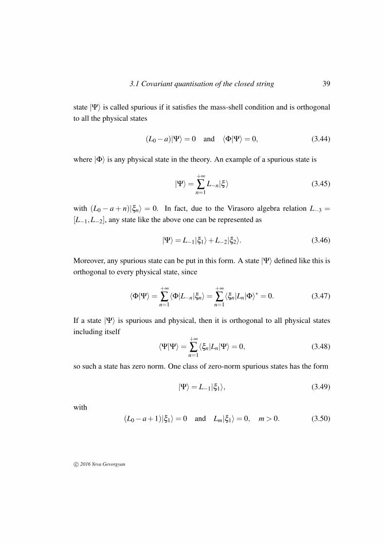
3.1 Covariant quantisation of the closed string 39
state |Ψ〉 is called spurious if it satisfies the mass-shell condition and is orthogonalto all the physical states
(L0−a)|Ψ〉= 0 and 〈Φ|Ψ〉= 0, (3.44)
where |Φ〉 is any physical state in the theory. An example of a spurious state is
|Ψ〉=+∞
∑n=1
L−n|ξ 〉 (3.45)
with (L0 − a + n)|ξn〉 = 0. In fact, due to the Virasoro algebra relation L−3 =
[L−1,L−2], any state like the above one can be represented as
|Ψ〉= L−1|ξ1〉+L−2|ξ2〉. (3.46)
Moreover, any spurious state can be put in this form. A state |Ψ〉 defined like this isorthogonal to every physical state, since
〈Φ|Ψ〉=+∞
∑n=1〈Φ|L−n|ξn〉=
+∞
∑n=1〈ξn|Ln|Φ〉∗ = 0. (3.47)
If a state |Ψ〉 is spurious and physical, then it is orthogonal to all physical statesincluding itself
〈Ψ|Ψ〉=+∞
∑n=1〈ξn|Ln|Ψ〉= 0, (3.48)
so such a state has zero norm. One class of zero-norm spurious states has the form
|Ψ〉= L−1|ξ1〉, (3.49)
with(L0−a+1)|ξ1〉= 0 and Lm|ξ1〉= 0, m > 0. (3.50)
c© 2016 Yeva Gevorgyan
40 Quantisation of the bosonic string
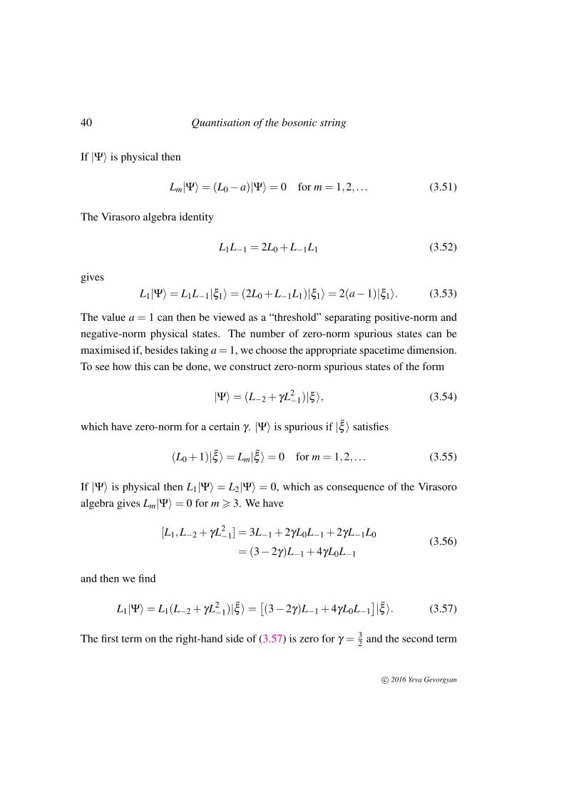
If |Ψ〉 is physical then
Lm|Ψ〉= (L0−a)|Ψ〉= 0 for m = 1,2, . . . (3.51)
The Virasoro algebra identity
L1L−1 = 2L0 +L−1L1 (3.52)
givesL1|Ψ〉= L1L−1|ξ1〉= (2L0 +L−1L1)|ξ1〉= 2(a−1)|ξ1〉. (3.53)
The value a = 1 can then be viewed as a “threshold” separating positive-norm andnegative-norm physical states. The number of zero-norm spurious states can bemaximised if, besides taking a= 1, we choose the appropriate spacetime dimension.To see how this can be done, we construct zero-norm spurious states of the form
|Ψ〉= (L−2 + γL2−1)|ξ 〉, (3.54)
which have zero-norm for a certain γ . |Ψ〉 is spurious if |ξ 〉 satisfies
(L0 +1)|ξ 〉= Lm|ξ 〉= 0 for m = 1,2, . . . (3.55)
If |Ψ〉 is physical then L1|Ψ〉 = L2|Ψ〉 = 0, which as consequence of the Virasoroalgebra gives Lm|Ψ〉= 0 for m > 3. We have
[L1,L−2 + γL2−1] = 3L−1 +2γL0L−1 +2γL−1L0
= (3−2γ)L−1 +4γL0L−1(3.56)
and then we find
L1|Ψ〉= L1(L−2 + γL2−1)|ξ 〉=
[(3−2γ)L−1 +4γL0L−1
]|ξ 〉. (3.57)
The first term on the right-hand side of (3.57) is zero for γ = 32 and the second term
c© 2016 Yeva Gevorgyan
3.2 Light-cone gauge quantisation 41
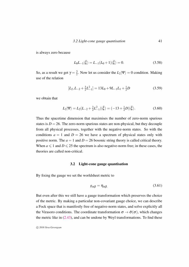
is always zero because
L0L−1|ξ 〉= L−1(L0 +1)|ξ 〉= 0. (3.58)
So, as a result we get γ = 32 . Now let us consider the L2|Ψ〉= 0 condition. Making
use of the relation
[L2,L−2 +32L2−1] = 13L0 +9L−1L1 +
12D (3.59)
we obtain that
L2|Ψ〉= L2(L−2 +32L2−1)|ξ 〉= (−13+ 1
2D)|ξ 〉. (3.60)
Thus the spacetime dimension that maximises the number of zero-norm spuriousstates is D = 26. The zero-norm spurious states are non-physical, but they decouplefrom all physical processes, together with the negative-norm states. So with theconditions a = 1 and D = 26 we have a spectrum of physical states only withpositive norm. The a = 1 and D = 26 bosonic string theory is called critical theory.When a 6 1 and D 6 25 the spectrum is also negative-norm free; in these cases, thetheories are called non-critical.
3.2 Light-cone gauge quantisation
By fixing the gauge we set the worldsheet metric to
gαβ = ηαβ . (3.61)
But even after this we still have a gauge transformation which preserves the choiceof the metric. By making a particular non-covariant gauge choice, we can describea Fock space that is manifestly free of negative-norm states, and solve explicitly allthe Virasoro conditions. The coordinate transformation σ → σ(σ), which changesthe metric like in (2.43), and can be undone by Weyl transformations. To find these
c© 2016 Yeva Gevorgyan
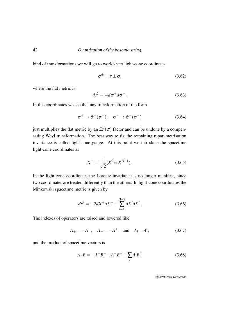
42 Quantisation of the bosonic string
kind of transformations we will go to worldsheet light-cone coordinates
σ± = τ±σ , (3.62)
where the flat metric isds2 =−dσ
+dσ−. (3.63)
In this coordinates we see that any transformation of the form
σ+→ σ
+(σ+), σ−→ σ
−(σ−) (3.64)
just multiplies the flat metric by an Ω2(σ) factor and can be undone by a compen-sating Weyl transformation. The best way to fix the remaining reparametrisationinvariance is called light-cone gauge. At this point we introduce the spacetimelight-cone coordinates as
X± =1√2(X0±XD−1). (3.65)
In the light-cone coordinates the Lorentz invariance is no longer manifest, sincetwo coordinates are treated differently than the others. In light-cone coordinates theMinkowski spacetime metric is given by
ds2 =−2dX+dX−+D−2
∑i=1
dX idX i. (3.66)
The indexes of operators are raised and lowered like
A+ =−A−, A− =−A+ and Ai = Ai, (3.67)
and the product of spacetime vectors is
A ·B =−A+B−−A−B++∑i
AiBi. (3.68)
c© 2016 Yeva Gevorgyan
3.2 Light-cone gauge quantisation 43
The equation of motion for X+ then becomes
∂+∂−X+ = 0, (3.69)
the general solution of which is
X+ = X+L (σ+)+X+
R (σ−). (3.70)
Now we must fix the gauge. Because of reparametrisation invariance, we can choosethe coordinates as
X+L =
12
x++12
α′p+σ
+, X+R =
12
x++12
α′p+σ
−. (3.71)
The outcome of this choice of gauge is that
X+ = x++α′p+τ. (3.72)
This gauge is called the light-cone gauge. Equation (3.72) fixes the reparametri-sation invariance, but may give rise to new conditions in addition to the alreadyexisting ones, namely,
(∂+X)2 = (∂−X)2 = 0. (3.73)
Now let us look at equation of motion for X−:
∂+∂−X− = 0. (3.74)
The general solution is given by
X− = X−L (σ+)+X−R (σ−). (3.75)
c© 2016 Yeva Gevorgyan
44 Quantisation of the bosonic string
This solution is completely determined by constraints (3.73). The first constraint is
2∂+X−∂+X+ =D−2
∑i=1
∂+X i∂+X i, (3.76)
which together with ∂+X+ = α ′p+ gives
∂+X−L =1
α ′p+D−2
∑i=1
∂+X i∂+X i, (3.77)
and
∂−X−R =1
α ′p+D−2
∑i=1
∂−X i∂−X i. (3.78)
So X−(σ+,σ−) is determined in terms of other fields up to an integration constant.Now we write the mode expansion for X−L,R as
X−L (σ+) =12
x−+12
α′p−σ
++ i
√α ′
2 ∑n 6=0
1n
α−n e−inσ+
, (3.79)
X−R (σ−) =12
x−+12
α′p−σ
−+ i
√α ′
2 ∑n 6=0
1n
α−n e−inσ−, (3.80)
where x− is an integration constant and p−, α−n , and α−n are found from (3.77) and(3.78). The oscillator modes are
α−n =
1√2α ′
1p′
+∞
∑n=−∞
D−2
∑i=1
αin−mα
im. (3.81)
A special case of this is
α ′
2p− =
12p+
D−2
∑i=1
(12
α′pi pi + ∑
n6=0α
inα
i−n
)(3.82)
c© 2016 Yeva Gevorgyan
3.2 Light-cone gauge quantisation 45
We also have an equation for p− in terms of α−0 ,
α ′
2p− =
12p+
D−2
∑i=1
(12
α′pi pi + ∑
n6=0α
inα
i−n
)(3.83)
from here we can write the string mass-shell condition
M2 =−pµ pµ = 2p+p−+D−2
∑i=1
pi pi
=4α ′
D−2
∑i=1
∑n>0
αi−nα
in =
4α ′
D−2
∑i=1
∑n>0
αi−nα
in.
(3.84)
3.2.1 Quantisation
To quantise the closed string we first have to impose commutation relations. Someare
[xi, p j] = iδ i j and [α in,α
jm] = [α i
n, αj
m] = nδi j
δn+m,0, (3.85)
which follow from (3.3) and (3.4). These commutation relations hold only whenwe are quantising physical degrees of freedom. For x+ and p− the commutationrelation is
[x+, p−] =−i. (3.86)
This relation means that we can choose states to be eigenstates of pµ , with µ =
0,1, . . . ,D− 1, but the constraints (3.82) and (3.83) must hold. We define thevacuum state |0; p〉 such that
pµ |0; p〉= pµ |0; p〉 and αin|0; p〉= α
in|0; p〉= 0 for n > 0, (3.87)
and the Fock space is built by acting on |0; p〉 with the operators α i−n and α i
−n forn> 0. The difference from covariant quantisation is that we act only with transverseoscillators which carry a spatial index i = 1, . . . ,D− 2. So the Hilbert space is
c© 2016 Yeva Gevorgyan
46 Quantisation of the bosonic string
positive defined and we do not have ghosts.
3.2.2 The constraints
p− is not an independent variable of the theory, and we have to impose constraints(3.82) and (3.83) to define physical states. In the classical theory this constaints arethe mass-shell conditions. But on the quantum level we have the problem of normalordering. If we choose all operators to be normal-ordered we will gain a constant a.In the same way as in previous sections we find the mass in the light-cone gauge as
M2 =4α ′
(D−2
∑i=1
∑n>0
αi−nα
in−a
)=
4α ′
(D−2
∑i=1
∑n>0
αi−nα
in−a
). (3.88)
Now we introduce the operators
N =D−2
∑i=1
∑n>0
αi−nα
in and N =
D−2
∑i=1
∑n>0
αi−nα
in, (3.89)
which resemble the number operators except that the summations in their definitionsexclude the time coordinate and one of the space coordinates (D− 1). With theseoperators we can write the mass of the string as
M2 =4α ′
(N−a) =4α ′
(N−a). (3.90)
This expression looks similar to the expression (3.41) that we got before for themass, just lucking some of the coordinates . Now the open question is how to fix a.We will try to answer this question in the next section.
3.2.3 The zeta function regularization
In this section our goal is to find a sensible value for the normal ordering constant athat appears in the expresions (3.41) and (3.90) for the mass of the string. We willdo this in a heuristic way.
c© 2016 Yeva Gevorgyan
3.2 Light-cone gauge quantisation 47
Let us look at the following classical result without normal ordering,
12 ∑
n 6=0α
i−nα
in =
12 ∑
n<0α
i−nα
in +
12 ∑
n>0α
i−nα
in, (3.91)
where we left the summation over i = 1, . . . ,D−2 implicit. Now we try to normal-order the above expressions by moving all α i
n, the annihilation operator, to the rightfor n > 0 and to the left for n < 0. The second term on the right-hand side ofequation (3.91) is already normal-ordered and we just have to adjust its first term,which gives
12 ∑
n<0[α i
nαi−n−n(D−2)]+
12 ∑
n>0α
i−nα
in = ∑
n>0α
i−nα
in +
12(D−2) ∑
n>0n. (3.92)
The last term in this expression diverges (badly!), but this divergence has a physicalinterpretation: it is the sum of the zero-point energies of an infinite number ofharmonic oscillators (which may or may not be observable). We may try to “sum”that term by by extension of so called zeta-function (see, e. g., [11]). The zeta-function is defined, for Re(s)> 1, by the sum
ζ (s) =∞
∑n=1
n−s.
But ζ (s) has a unique analytic continuation to all values of s. In particular
ζ (−1) =− 112
.
Due to this result sum in equation (3.92) is(2)
+∞
∑n=1
n =− 112
. (3.93)
(2)This “result” is clearly outragious out of its context and should not be taken at face value!
c© 2016 Yeva Gevorgyan
48 Quantisation of the bosonic string
In agreement with the last result we must have a = − 124
(D− 2), which togetherwith equation (3.90) gives
M2 =4α ′
(N− D−2
24
)=
4α ′
(N− D−2
24
)(3.94)
for the mass of the closed relativistic bosonic string.
3.3 The string spectrum
In this section we will analyse the spectrum of a free closed single string.
3.3.1 The tachyon
We want to find the mass-shell constraint. Let us start with the ground state |0; p〉defined in equation (3.87). If we do not have excited oscillators, N = 0 and
M2 =− 1α ′
D−26
. (3.95)
We got for any D > 2 a negative mass-squared. We call these kind of hypotheticalparticles with negative mass-squared tachyons. In the special theory of relativity,tachyons can be interpreted as particles that travel faster than light. Let us brieflydiscuss the QFT interpretation for the tachyons. Suppose that we have a field T (X)
in spacetime whose quanta give rise to tachyons. In this case, the mass-squared ofthe particle can be expressed as
M2 =∂ 2V (T )
∂T 2
∣∣∣∣T=0
. (3.96)
The negative mass-squared for the tachyon shows that we are expanding around amaximum of the potential V (T ) for the tachyon field. The string theory thus sitson an unstable point, and we do not know if the potential has a good minimumpoint elsewhere. So the real behaviour of the tachyon in the bosonic string theory
c© 2016 Yeva Gevorgyan
3.3 The string spectrum 49
is tricky. But tachyons do not cause problems in fermionic string theory, which willnot be discussed.
3.3.2 First excited states
Let us now look at the first excited states of the theory. To get them we first act on|0; p〉 with a creation operator α
j−1, then equation (3.90) tells us that we need also
to act with the operator α i−1. So we have (D−2)2 particles in the first excited state
given byα
i−1α
j−1|0; p〉, (3.97)
each one with mass-squared
M2 =4α ′
(1− D−2
24
). (3.98)
Here we seem to be in trouble. The operators α i and α i each transform in the vectorrepresentation of SO(D−2)⊂ SO(1,D−1) which is manifest in light-cone gauge.But we want these states to fix into some full representation of the Lorentz groupSO(1,D− 1). As we already mentioned in Sec. 3.2, it is not easy to see Lorentzinvariance in the light-cone gauge. To continue, we will use Wigner’s classificationof representations of the Poincaré group. First we have massive particles in R1,D−1,where R1,D−1 is the group of translations. When we go to the rest frame of theparticle by setting pµ = (p,0, . . . ,0), we can watch how any internal index trans-forms under the little group SO(D− 1) of spatial rotations. As a consequence anymassive particle must form a representation of SO(D− 1). But particles describedby equation (3.97) have (D− 2)2 states. We cannot pack (D− 2)2 states into theSO(D− 1) representation, so the first excited states of the string cannot form amassive representation of the D-dimensional Poincaré group. The way out fromthis situation is to pick massless states, but then we cannot go to the rest frame. Wecan just set a spacetime momentum for the particle to the form pµ = (p,0, . . . ,0, p).In this case particles represent the little group SO(D−2), so massless particles haveless internal states than the massive ones. The first excited states (3.97) sit in a
c© 2016 Yeva Gevorgyan
50 Quantisation of the bosonic string
representation of SO(D−2). And if we want quantum theory to preserve the initialSO(1,D− 1) Lorentz symmetry, the first excited states should be massless. UsingM2 = 0 and equation (3.98) we get
D = 26,
which is the critical dimension of the bosonic string.
3.3.3 Higher excited states
We kept the Lorentz invariance of the first excited states by choosing D = 26, tomake the states massless. For the higher excited states we still have indexes in therange i, j = 1, . . . ,D−2 = 24. From equation (3.94) all the higher excited states aremassive, and must form representation of SO(D− 1). Let us see what we can dothis time. Let us look at the string at level N = N = 2. In the right-moving sector wehave two states: α i
−1αj−1|0〉 and α i
−2|0〉. The same holds in the left-moving sector,so we have in total (
αi−1α
j−1⊕α
i−2)⊗(α
i−1α
j−1⊕ α
i−2)|0; p〉 (3.99)
states. These states have mass M2 = 4/α ′. In the left-moving sector we have
12(D−2)(D−1)+(D−2) =
12
D(D−1)−1 (3.100)
states, which fit into the SO(D− 1) representation. So after we fix D = 26, theLorentz invariance is preserved for all the excited states. We conclude that toquantise the bosonic string in the light-cone gauge we have to set
a = 1 and D = 26. (3.101)
c© 2016 Yeva Gevorgyan
4
Conformal field theory and strings
In this chapter we introduce the two dimensional conformal field theories and theirconnection with strings. The ideas and techniques presented here are used in theBRST quantisation of the string. We draw our notes mostly from the books byBecker, Becker and Schwartz [9] and by Polchinsky [14].
4.1 Introduction to conformal field theory
A conformal field theory is a theory that is invariant under conformal transforma-tions. We introduce conformal transformations as changes of coordinates σα(σ)→σα(σ) under which the metric transforms as
gαβ (σ)→Ω2(σ)gαβ (σ). (4.1)
We already encountered a particular case of these transformations earlier; see (2.43).Looking at the transformations we conclude that the theory is rescaling invariant butis sensitive to the change of angles. The transformations (4.1) can have differentinterpretations. If gαβ (σ) is a dynamical metric, we have a gauge symmetry. Ifgαβ (σ) is fixed, the transformation is physical, and we have a global symmetrywith conserved currents. For the Polyakov action the metric is dynamical and thetransformations (4.1) are residual gauge transformations, which can be undone byapplying the Weyl transformations. Conformal field theory is a subset of QFT, butsince the theory does not have a preferred length scale, it is true only for masslessexcitations.
51
52 Conformal field theory and strings
4.1.1 Euclidean worldsheet
It is simpler to deal with CFT on Euclidean worldsheets. To go from a Minkowkiworldsheet to an Euclidean worldsheet we use a Wick rotation σ0 → iσ0. On anEuclidean worldsheet, the metric gαβ is positive definite. The Euclidean worldsheetcoordinates are defined as (σ1,σ2) = (σ1, iσ0). We also have complex worldsheetcoordinates defined as
z = σ1 + iσ2 and z = σ
1− iσ2; (4.2)
they are analogue of the light-cone coordinates. The holomorphic and antiholomor-phic derivatives are given, respectively, by
∂z = ∂ =12(∂1− i∂2) and ∂z = ∂ =
12(∂1 + i∂2). (4.3)
We will usually work in flat Euclidean space with the metric
ds2 = (dσ1)2 +(dσ
2)2 = dzdz. (4.4)
In components the metric tensor gαβ can be written as (1)
gzz = gzz = 0 and gzz = gzz =12. (4.5)
On the Euclidean worldsheet the delta function is defined as∫d2zδ (z, z) = 1, (4.6)
(1)We use (4.2) and (4.3) to calculate the components of the metric tensor:
gzz = gzz = ∂zσµ
∂zσν gµν = ∂zσ
1∂zσ
1 +∂zσ2∂zσ
2 =14+
14=
12.
By the same token, gzz = gzz = 0.
c© 2016 Yeva Gevorgyan
4.1 Introduction to conformal field theory 53
and the expression∫
d2σδ (σ) = 1 is also satisfied. Vectors in this space are definedas
vz = (v1 + iv2) and vz = (v1− iv2), (4.7)
for the upper indices, and
vz =12(v1− iv2) and vz =
12(v1 + iv2), (4.8)
for the lower indices.
4.1.2 The conformal group in D dimensions
A D-dimensional manifold is called conformally flat if the metric element reads
ds2 = eω(x)dx ·dx, (4.9)
where ω(x) is allowed to be x-dependent. The conformal group is the subgroupof the group of general transformations that preserves the conformal flatness of themetric. Conformal transformations preserve the angles and distort the lengths. Theconformal group contains four types of transformations:
Translations: xµ → xµ +aµ , with aµ constant. For the infinitesimal case δxµ = aµ ,where aµ is an infinitesimal constant.
Rotations: xµ → ωµ
ν xµ . This transformation is the same for finite and infinitesimalcases, but for infinitesimal rotations ω
µ
ν is an infinitesimal constant obeying ωµν =
−ωνµ .
Scale transformations: xµ → λxµ . This transformation is also the same for finiteand infinitesimal cases; in the infinitesimal case λ is an infinitesimal constant.
Special conformal trasformations: The conformal group includes inversions,
xµ → xµ
x2 , (4.10)
c© 2016 Yeva Gevorgyan
54 Conformal field theory and strings
which maps
dx ·dx→ dx ·dx(x2)2 , (4.11)
so that the metric remains conformally flat. If we perform a sequence of inversion,translation, and inversion again we then obtain the special conformal transformation
xµ → xµ +bµx2
1+2bx+b2x2 . (4.12)
If bµ is infinitesimal, we have
δxµ = bµx2−2xµbx. (4.13)
Taken together, these transformations mean that the following infinitesimaltransformations are conformal,
δxµ = aµ +ωµ
ν xν +λxµ +bµx2−2xµ(b · x), (4.14)
with the parameters aµ ,ωµ
ν ,λ and bµ infinitesimal constants. Altogether we have
D+12
D(D−1)+1+D =12(D+2)(D+1) (4.15)
linearly independent infinitesimal conformal transformations, so this is the numberof generators of the conformal group. The conformal group for D > 2 Euclideandimensions is the indefinite special orthogonal group SO(D+1,1).
4.1.3 Conformal transformations in two dimensions
Conformal transformations of the flat space are
z→ z′ = f (z) and z→ z′ = f (z), (4.16)
c© 2016 Yeva Gevorgyan
4.1 Introduction to conformal field theory 55
which are any holomorphic change of the coordinates. Under this transformationsthe metric transforms as
ds2 = dzdz→∣∣∣∣d f
dz
∣∣∣∣2 dzdz (4.17)
which is of form (4.1). The infinitesimal conformal trasformations are of the form
z→ z′ = z− εzn+1 and z→ z′ = z− εnzn+1, (4.18)
such that for each n ∈ Z we have the following infinitesimal generators
ln =−zn+1∂ and ln =−zn+1
∂ . (4.19)
Since n ∈ Z we have an infinite number of conformal transformations, which istypical for two dimensions. In higher dimensions, the space of conformal trans-formations is a finite dimensional group. These generators satisfy the classicalVirasoro algebra
[lm, ln] = zm+1∂z(zn+1
∂z)− zn+1∂z(zm+1
∂z) =
= (n+1)zm+n+1∂z− (m+1)zn+m+1
∂z =
=−(m−n)zm+n+1∂z = (m−n)lm+n,
(4.20)
and in the same way
[lm, ln] = (m−n)lm+n, and [lm, ln] = 0. (4.21)
As already had been told in previous chapters, in the quantum case the Virasoroalgebra acquire a central extension
[Lm,Ln] = (m−n)Lm+n +c
12m(m2−1)δm+n,0, (4.22)
c© 2016 Yeva Gevorgyan
56 Conformal field theory and strings
with c the central charge. In two dimensions the Virasoro operators are the modesof the energy-momentum tensor, which generates the conformal transformations.Central extension means that the constant term is multiplying the unit operator,which is adjoined to the Lie algebra. The infinite-dimensional conformal group intwo dimensions contains a finite-dimensional subgroup generated by l0,±1 and l0,±1,infinitesimally from (4.18) the transformations are
l−1 : z→ z− ε,
l0 : z→ z− εz,
l1 : z→ z− εz2.
(4.23)
The finite form of the group transformations is
z→ az+bcz+d
with a,b,c,d ∈ C, ad−bc = 1. (4.24)
This transformation is invariant under the change of signs of all parameters, so thisis the group of projective conformal transformations SL(2,C)/Z2 = SO(3,1), whichis the two-dimensional case of SO(D+1,1), where D > 2. The finite-dimensionalsubgroup of the two-dimensional infinite conformal group is called the restrictedconformal group.
4.2 Classical aspects of CFT
We will see some aspects of classical theories that are invariant under conformaltransformations.
4.2.1 The stress-energy tensor
The stress-energy (or energy-momentum) tensor is very important for any fieldtheory. The energy-momentum tensor is a matrix of conserved currents arisingfrom translational invariance δσα = εα , with εα an infinitesimal constant.
c© 2016 Yeva Gevorgyan

4.2 Classical aspects of CFT 57
Let us derive the stress-energy tensor in the general case, supposing that weare in a flat space, with gαβ = ηαβ . To derive conserved currents we take ε = ε(σ)
a function of the spacetime coordinates. Then the change in the action must be
δS =∫
d2σJα
∂αε (4.25)
for some function Jα , which depends on the fields involved. δS should vanish forconstant ε . If the equations of motion are satisfied, we must have δS = 0 for anyε(σ). This means that
∂αJα = 0, (4.26)
so that the Jα are conserved.
Now we will look at translational invariance. If ε becomes a function of theworldsheet coordinates, the action changes as in (4.25). To find what Jα is in thiscase, we consider a coupling to a dynamical background metric gαβ (σ). We knowthat in this case the theory is invariant under the transformation
δσα = ε
α(σ), (4.27)
as long as the metric also changes simultaneously by
δgαβ = ∂αεβ +∂β εα . (4.28)
Due to the last statement we have
δS =−∫
d2σ
∂S∂gαβ
=−2∫
d2σ
∂S∂gαβ
∂αεβ . (4.29)
Now we have a new translational constant, which with some coefficient will becalled stress-energy tensor
Tαβ =− 4π√
g∂S
∂gαβ. (4.30)
c© 2016 Yeva Gevorgyan
58 Conformal field theory and strings
On a curved worldsheet the energy-momentum tensor is covariantly conserved
∇αTαβ = 0; (4.31)
the proof of (4.31) is given in Appendix A. S is invariant under infinitesimal Weyltransformations, which transform only the metric, δgαβ =−δλgαβ . From here wecan prove that the stress-energy tensor is traceless,
0 =− 4π√
gδSδλ
=− 4π√
gδS
δgαβ
δgαβ
δλ= Tαβ gαβ = T α
α . (4.32)
We can see the same in the complex coordinates:
Tzz =∂σα
∂ z∂σβ
∂ zTαβ =
=∂σ1
∂ z∂σ1
∂ zT11 +
∂σ2
∂ z∂σ1
∂ zT21 +
∂σ1
∂ z∂σ2
∂ zT12 +
∂σ2
∂ z∂σ2
∂ zT22 =
=14(T11 +T22) = 0.
(4.33)
The conservation conditions (4.31) can be written as
∂Tzz = 0 and ∂Tzz = 0. (4.34)
So, there are just two non-vanishing components of the stress-energy tensor, oneholomorphic Tzz = Tzz(z) and one antiholomorphic Tzz = Tzz(z). In the new notationwe can write the mode expansion for the closed string as
X µ
R (σ ,τ)→ X µ
R (z) =12
xµ − i4
pµ lnz+i2 ∑
n6=0
1n
αµn z−n, (4.35)
andX µ
L (σ ,τ)→ X µ
L (z) =12
xµ − i4
pµ ln z+i2 ∑
n6=0
1n
αµn z−n; (4.36)
c© 2016 Yeva Gevorgyan
4.2 Classical aspects of CFT 59
for the holomorphic derivatives we have
∂X µ(z, z) =− i2
+∞
∑n=−∞
αµn z−n−1, (4.37)
and
∂X µ(z, z) =− i2
+∞
∑n=−∞
αµn z−n−1. (4.38)
We can find the holomorphic component of the energy-momentum tensor as
TX(z) =−2 : ∂X ·∂X :=+∞
∑n=−∞
Ln
zn+2 . (4.39)
while for the antiholomorphic component we find
TX(z) =−2 : ∂X · ∂X :=∞
∑n=−∞
Ln
zn+2 . (4.40)
4.2.2 Noether currents
The stress-energy tensor provides the Noether currents for translation. Now weneed to see how they look for other conformal transformations. Let us suppose thatwe have an infinitesimal change
z′ = z+ ε(z), z′ = z+ ε(z); (4.41)
when ε is constant we have translations, while ε(z)∼ z corresponds to rotations anddilatations. We again go from ε(z)→ ε(z, z). In this case the action changes like
δS =−∫
d2σ
∂S∂gαβ
δgαβ =1
2π
∫d2
σTαβ (∂α
δσβ ). (4.42)
Since in a conformal theory Tzz = 0,
δS =1
2π
∫d2z
12[Tzz(∂
zδ z)+Tzz(∂
zδ z)]=
12π
∫d2z[Tzz∂zε +Tzz∂zε
]. (4.43)
c© 2016 Yeva Gevorgyan
60 Conformal field theory and strings
If ε is holomorphic and ε is antiholomorphic then δS = 0, which means that wehave a symmetry. Let us treat z and z as independent variables. First we look atsymmetry
δ z = ε(z), δ z = 0. (4.44)
Since ε already depends on z, we go from ε(z)→ ε(z) f (z) for some function f . Inthis case
δS =1
2π
∫d2z[Tzzε(z)∂z f (z)], (4.45)
so thatJz = 0 and J z = Tzzε(z) (4.46)
and we see that J is holomorphic. For the case of symmetry
δ z = ε(z), δ z = 0 (4.47)
we getJz = Tzz(z)ε(z) and J z, (4.48)
with an antiholomorphic current J.
4.3 Quantum aspects of CFT
In this section we will discuss some aspects of quantum theories that are preservedunder conformal transformations.
4.3.1 Operator product expansion
In CFT the term field refers to any local expression that we can write down. Thisincludes Φ, but also ∂ nΦ and composite operators such as eiΦ. All these aredifferent fields in a CFT. The number of fields in CFT is infinite.
Let Oi be a set of all local operators in a CFT. Two local operators insertedat nearby points can be closely approximated by a string of operators at one of these
c© 2016 Yeva Gevorgyan
4.3 Quantum aspects of CFT 61
points. We call such an approximation as an operator product expansion, or OPE.The OPE for two operators is given by
Oi(z, z)O j(ω, ω) = ∑k
cki j(z−ω, z− ω)Ok(ω, ω), (4.49)
where cki j(z−ω, z− ω) are a set of functions which depend only on the separation
between the two operators. Equations of type (4.49) are statements which hold asoperator insertions inside time-ordered corelation functions,
〈Oi(z, z)O j(ω, ω) · · · 〉= ∑k
cki j(z−ω, z− ω)〈Ok(ω, ω) · · · 〉 (4.50)
where the · · · can be any operator insertion that we choose. Important aspects ofOPEs are:
• The correlation functions are always time-ordered—as far as the OPE is con-cerned, everything commutes, Oi(z, z)O j(ω, ω) = O j(ω, ω)Oi(z, z) (exceptfor Grassmann objects, which get a minus sign).
• Operator insertions are arbitrary, but they should be a distance large comparedto |z−ω|. So in a CFT the OPEs are exact statements and have a radius ofcovergence equal to the distance to the nearest insertion. OPEs have singularbehaviour as z→ ω .
• OPEs contain the same information as the commutation relations, and alsotell us the way operators transform under symmetries.
4.3.2 Ward identities
Ward identities are operator analogs to Noether’s theorem in quantum field theories.Let us derive them in a general theory with a symmetry. We will use the partitionfunction of the field theory written as a path integral,
Z =∫
Dφe−S[φ ], (4.51)
c© 2016 Yeva Gevorgyan
62 Conformal field theory and strings
where φ stands for all fields in a path integral sense. The quantum symmetry shouldbe such that an infinitesimal translation
φ′ = φ + εδφ (4.52)
keeps the action and the measure invariant
S[φ ′] = S[φ ] and Dφ′ = Dφ . (4.53)
If we promote ε→ ε(σ), the action and the measure do not stay invariant anymore,but to leading order in ε , the change is proportional to ∂ε . In this case
Z→∫
Dφ′ exp(−S[φ ′])
=∫
Dφ exp(−S[φ ′]− 12π
∫d2
σ√
gJα∂αε)
=∫
Dφe−S[φ ](1− 12π
∫d2
σ√
gJα∂αε);
(4.54)
here Jα can have contributions from the measure transformation. The integral forthe partition function changed but the function itself could not change, so we mustensure that
Z′−Z = 0. (4.55)
More explicitly, ∫Dφe−S[φ ]]
(∫d2
σ√
gJα∂αε
)= 0. (4.56)
Since this condition must hold for all ε , the vacuum expectation value of the diver-gence of the current must vanish
〈∂αJα〉= 0. (4.57)
Let us see the result when we have other insertions in the path integral. Let Oi
be any general expressions formed from the φ fields. Under a given symmetry
c© 2016 Yeva Gevorgyan
4.3 Quantum aspects of CFT 63
transformation they will change like
Oi→ Oi + εδOi. (4.58)
We again go from ε → ε(σ). Let us pick ε(σ) such as all Oi(σi) are far from theoperator insertions, in this case
δOi(σi) = 0. (4.59)
And the derivation is the same as in the first case, which gives
〈∂αJα(σ)O1(σ1) · · ·On(σn)〉= 0 for σ 6= σi. (4.60)
Because this is true for operator insertions far from σ , we have
∂αJα = 0. (4.61)
Now let us see the case when some of the operators are in the same point as Jα . Letus suppose that ε(σ) is in the same region only with σ1. We put ε(σ) constant inthis region, and zero in the outside of it. Now the original correlation function is
1Z
∫Dφe−S[φ ]
(1− 1
2π
∫d2
σ√
gJα∂αε
)(O1 + εδO1)O2 · · ·On. (4.62)
In leading order in ε it gives
− 12π
∫ε
d2σ√
g∂α〈Jα(σ)O1(σ1) · · · 〉= 〈δO1(σ1) · · · 〉 (4.63)
with the integral over non-zero ε . This is the Ward identity.
c© 2016 Yeva Gevorgyan
64 Conformal field theory and strings
Ward identities for conformal transformations
Ward identities hold for all types of symmetries. Let us see what happens forconformal transformation in two dimensions. Let nα be the unit vector normalto the boundary. Then for any Jα , we have, by Stokes’ theorem [15],∫
ε
∂αJα =∮
∂ε
Jα nα =∮
∂ε
(J1dσ2− J2dσ
1) =−i∮
∂ε
(Jzdz− Jzdz), (4.64)
both in Cartesian and complex coordinates. For complex coordinates we use thenotation
Jz =12(J1− iJ2) and Jz =
12(J1 + iJ2). (4.65)
Using (4.64) for Ward identities we get
i2π
∮∂ε
dz〈Jz(z, z)O1(σ1) · · · 〉−i
2π
∮∂ε
dz〈Jz(z, z)O1(σ1) · · · 〉= 〈δO1(σ1) · · · 〉.(4.66)
This holds for any J in two dimensions. Now we go to the currents (4.46, 4.48)found for conformal transformations. Jz is holomorphic and Jz is antiholomorphic,so by the residue theorem we get
i2π
∮∂ε
dzJz(z)O1(σ1) =−Res [JzO1]. (4.67)
Using last equation we can write the OPE of the two operators as
Jz(z)O1(ω.ω) = · · ·+ Res [JzO1(ω, ω)]
z−ω+ · · · . (4.68)
Now if we treat z and z as independent variables, we will have a Ward identity intwo parts. For δ z = ε(z),
δO1(σ1) =−Res [Jz(z)O1(σ1)] =−Res [ε(z)TzzO1(σ1)], (4.69)
c© 2016 Yeva Gevorgyan
4.3 Quantum aspects of CFT 65
and for ε z = ε(z)
δO1(σ1) =−Res [Jz(z)O1(σ1)] =−Res [ε(z)Tzz(z)O1(σ1)]. (4.70)
So if we know the OPE between an operator and the stress-energy tensor T (z) andTzz(z), we know how the operator transforms under the conformal symmetry.
4.3.3 Primary operators
In this section we will discuss some tipes of OPEs. Let us start from some simplecases of conformal symmetries.
Translations: δ z = ε = constant. For infinitesimal translation all operators trans-form as
O(z− ε) = O(z)− ε∂O(z)+ · · · . (4.71)
The Noether current Jz(z) for the translation is the stress-energy tensor T . Usingequation (4.68) and analogues of equations (4.69,4.70) with Jz(z) = T , we concludethat OPE of T with any operator O must be
T (z)O(ω, ω) = · · ·+ ∂O(ω, ω)
z−ω+ · · · , (4.72)
and for T by analogy
T (z)O(ω, ω) = · · ·+ ∂O(ω, ω)
z− ω+ · · · . (4.73)
Rotation and scaling: This are the transformations of form
z→ z+ εz and z→ z+ ε z, (4.74)
which present rotations for imaginary ε and dilatations for real ε . Not all the op-erators have good transformation properties under these transformations. We state
c© 2016 Yeva Gevorgyan
66 Conformal field theory and strings
that we always can choose a basis of local operators that have good transformationproperties under rotations and dilatations.
It is said that an operator O has weight (h, h) if, under δ z = εz and δ z = ε z ittransforms as
δO =−ε(hO+ z∂O)− ε(hO+ z∂O). (4.75)
The terms with ∂O are general terms, and terms hO and hO are special to operatorswhich are eigenstates of dilatations and rotations.
Let us make some comments about the last definition.
• h and h are real numbers; for all operators in a unitary CFT h, h > 0.
• The eigenvalue under rotation is the “old friend” spin given by s = h− h. Thescaling dimension ∆ of an operator is ∆ = h+ h.
• Rotation acts on the underlying coordinates as
L = i(σ1∂2−σ
2∂1) = z∂ + z∂ .
Dilatation acts on the underlying coordinates as the Dilaton operator
D = σα
∂α = z∂ + z∂ .
• The rescaling dimension ∆ is the common one found for the fields and oper-ators by the use of dimensional analysis—for example, ∆[∂ ] = +1—but wehave to remember that the quantum dimension is not always the same as theclassical one.
The Noether current Jz(z) for the translation is zT . Using equation (4.68) andanalogues of equations (4.69,4.70) with Jz(z) = zT , we conclude that OPE of Twith any operator O must be
T (z)O(ω, ω) = · · ·+hO(ω, ω)
(z−ω)2 +∂O(ω, ω)
z−ω+ · · · , (4.76)
c© 2016 Yeva Gevorgyan
4.3 Quantum aspects of CFT 67
and for T by the analogy
T (z)O(ω, ω) = · · ·+ hO(ω, ω)
(z− ω)2 +∂O(ω, ω)
z− ω+ · · · . (4.77)
Primary operators
A primary operator is one that has OPE that does not have singularities in higherorder than (z−ω)−2 for T and (z− ω)−2 for T . This means we know all thesingularities in the OPE of TO, such that we can see the transformation under allconformal transformations. For δ z = ε(z) transformation
δO(ω, ω) =−Res [εzT (z)O(ω, ω)]
=−Res[
ε(z)(
hO(ω, ω)
(z−ω)2 +∂O(ω, ω)
z−ω+ · · ·
)] (4.78)
We require ε(z) not to have singularities at z = ω . Then we can Taylor expand it
ε(z) = ε(ω)+ ε′(ω)(z−ω)+ · · · . (4.79)
Using the expansion we find the infinitesimal change of a primary operator under ageneral conformal transformation δ z = ε(z)
δO(ω, ω) =−hε′(ω)O(ω, ω)− ε(ω)∂O(ω, ω), (4.80)
and the simulat equation for the antiholomorphic transformations δ z = ε(z). Thementioned equations hold for infinitesimal conformal transformations. For generaltransformation z→ z(z) and z→ ¯z(z) of a primary operator we have
O(z, z)→ O(z, ¯z) =(
∂ z∂ z
)−h(∂ ¯z∂ z
)−h
O(z, z). (4.81)
The spectrum of weights (h, h) of primary fields is one of main interests of CFT.
c© 2016 Yeva Gevorgyan
68 Conformal field theory and strings
4.4 The central charge
The stress-energy tensor is not a primary operator. T is an operator of weight(h, h) = (2,0) in any CFT, because Tαβ has dimension ∆ = h+ h = 2, because weobtain the energy by integrating over space, and it has spin s = h− h = 2 because itis asymmetric 2-tensor. Similarly T has weight (0,2). So the T T OPE is
T (z)T (ω) = · · ·+ 2T (ω)
(z−ω)2 +∂T (ω)
z−ω+ · · · . (4.82)
The same for T T . Since each term in the equation has dimension ∆ = 4, we canonly have operators of the form
On
(z−ω)n ,
where ∆[Om] = 4−n. But as we stated before in unitary CFT there are no operatorswith h, h < 0. So we can have only singular term of order (z−ω)−4, it gets into theOPE with some constant coefisient. So the T T OPE can be written as
T (z)T (ω) =c/2
(z−ω)4 +2T (ω)
(z−ω)2 +∂T (ω)
z−ω+ · · · , (4.83)
and the same for T T
T (z)T (ω) =c/2
(z− ω)4 +2T (ω)
(z− ω)2 +∂ T (ω)
z− ω+ · · · . (4.84)
c and c are the central charges, we can guess that they measure the number ofdegrees of freedom of the theory. Let us now see why we do not have singularterm of order (z−ω)−3. The reason is that for the OPE T (z)T (ω) = T (ω)T (z),because T T is included in the correlation functions, and they are time ordered.But the term proportional to (z−ω)−3 is not invariant under z ↔ ω . Now wewill see why (z−ω)−1 term is invariant under z↔ ω . We Taylor expand T (z) =T (ω)+(z−ω)∂T (ω)+ · · · and ∂T (z) = ∂T (ω)+ · · · , and put in equation (4.83),
c© 2016 Yeva Gevorgyan
4.4 The central charge 69
which gives
T (ω)T (z) =c/2
(z−ω)4 +2T (ω)+2(z−ω)∂T (ω)
(z−ω)2 − ∂T (ω)
z−ω= T (z)T (ω). (4.85)
We saw that equation (4.83) is indeed the full equation fot T T OPE.
The transformation of energy
Let us see how T transforms.
δT (ω) =−Res [ε(z)T (z)T (ω)]
=−Res[
ε(z)(
c/2(z−ω)4 +
2T (ω)
(z−ω)2 +∂T (ω)
z−ω+ · · ·
)].
(4.86)
If ε(z) has no singularities, we expand
ε(z) = ε(ω)+ ε′(ω)(z−ω)+
12
ε′′(ω)(z−ω)2 +
16
ε′′′(ω)(z−ω)3 + · · · , (4.87)
from which we find infinitesimal transformation of T
δT (ω) =−ε(ω)∂T (ω)−2ε′(ω)T (ω)− c
12ε′′′(ω). (4.88)
And for finite conformal transformation z→ z(z) T transforms as
T (z) =(
∂ z∂ z
)−2 [T (z)− c
12S(z,z)
], (4.89)
where S(z,z) is known as the Schwarzian derivative, given by
S(z,z) =(
∂ 3z∂ z3
)(∂ z∂ z
)−1
− 32
(∂ 2z∂ z2
)2(∂ z∂ z
)−2
. (4.90)
c© 2016 Yeva Gevorgyan
70 Conformal field theory and strings
4.4.1 The Weyl anomaly
In the classical theory T αα = 0. The story is different in the quantum case. On the
flat space 〈T αα 〉 also vanishes, but on a curved background it does not. We will try
to show that in curved space
〈T αα 〉=−
c12
R, (4.91)
where R is the Ricci scalar of the 2-dimensional worldsheet. Before derivation letus make some coments:
• Equation (4.91) holds for any state of the theory. This comes from the fact that〈T α
α 〉 regulates short distance divergences in the theory, and on short distanceall finite energies are basically the same.
• Since (4.91) is true for any state it should be something that depends onlyon the background metric. This something should be local and with ∆ = 2.The only candidate is the Ricci scalar R. But we do not know with whichcoeficient.
• Any 2-dimensional metric can be written as gαβ = e2ωδαβ . In these coordi-nates R =−2e−2ω∂ 2ω . So R depends on ω explicitely. Equation (4.91) tellsthat any conformal theory with c 6= 0 has at least one physical observable〈T α
α 〉, which takes different values on background related by Weyl transfor-mation ω . This result is called Weyl anomaly.
• In 4-dimensions there is also a Weyl anomaly
〈T µ
µ 〉4d =c
16π2 cρσκλ cρσκλ − a16π2 Rρσκλ Rρσκλ , (4.92)
with c the Weyl tensor and R the dual of the Riemann tensor.
• Equation (4.91) is in the left-moving sector, but we also have the equation〈T α
α =− c12R〉 in the right-moving sector. But for consistency in fixed curved
c© 2016 Yeva Gevorgyan

4.4 The central charge 71
backgrounds c = c. This is a gravitational anomaly.
Now let us prove equation (4.91). First we need to derive Tzz− Tωω OPE. Fromenergy conservation
∂Tzz =−∂Tzz
Using this
∂zTzz(z, z)∂ωTωω(ω, ω) = ∂zTzz(z, z)∂ωTωω(ω, ω) = ∂z∂ω
[c/2
(z−ω)4 + · · ·].
(4.93)In the last equation we have an antiholomorphic derivative of a holomorphic func-tion, which is supposed to be zero, but since we have singularities in T it is not.Using the fact that ∂z∂z|z−ω|2 = ∂z
1z−ω
= 2πδ (z−ω, z− ω)(2)
∂z∂ω
1(z−ω)4 =
16
∂z∂ω
(∂
2z ∂ω
1z−ω
)=
π
3∂
2z ∂ω ∂ωδ (z−ω, z− ω). (4.94)
Putting the last result into equation (4.93) we get rid of derivatives ∂z∂ω on bothsides. And finally we get
Tzz(z, z)Tω,ω(ω, ω) =cπ
6∂z∂ωδ (z−ω, z− ω), (4.95)
(2)The proof comes from the fact that ∂ 2 ln(σ −σ ′)2 = 4πδ (σ −σ ′), just with a correction factorof 2. If we set σ ′ = 0 and integrate over d2σ on the right-hand side we get∫
d2σ4πδ (σ) = 4π,
and applying Stokes’ theorem on the left-hand side we find∫d2
σ∂2 ln(σ2
1 +σ22 ) =
∫d2
σ∂α
(2σα
σ21 +σ2
2
)= 2
∮σ1dσ2−σ2dσ1
σ21 +σ2
2.
In polar coordinates σ1 + iσ2 = reiθ and∫d2
σ4πδ (σ) = 2∫ r2dθ
r2 = 4π,
and our statement is proved.
c© 2016 Yeva Gevorgyan
72 Conformal field theory and strings
which is zero except for the singularity z→ ω . It is a contact term between oper-ators. Let us now see how 〈T α
α 〉 changes under ageneral shift of the metrioc δgαβ
Using the deffinition of the energy-momentum tensor (4.30), we have
δ 〈T αα (σ)〉= δ
∫Dφe−ST α
α (σ) =
=1
4π
∫Dφe−S(T α
α (σ)∫
d2σ′√gδgβγTβγ(σ
′)).(4.96)
If we change to a Weyl transformation, the change to flat metric is δgαβ = 2ωδαβ ,so the change in the inverse metric is δgαβ =−2ωδ αβ , which gives
δ 〈T αα (σ〉) =− 1
2π
∫Dφe−S(T α
α (σ)∫
d2σ′ω(σ ′)T β
β(σ ′)). (4.97)
Now using equation (4.95) we will determine the Weyl anomaly. To do so wechange from complex to Cartesian coordinates. We have
T αα (σ)T β
β(σ) = 16Tzz(z, z)Tωω(ωω),
and8∂z∂ωδ (z−ω, z− ω) =−∂
2δ (σ −σ
′).
Together with (4.95) this gives
T αα (σ)T β
β(σ ′) =−cπ
3∂
2δ (σ −σ
′) (4.98)
this OPE in cartesian coordinates. Now putting it into equation (4.97) and integrat-ing by parts gives
δ 〈T αα 〉=
c6
∂2ω.
using that R = −2e−2ω∂ 2ω and putting e−2ω ≈ 1 since we are discussing an in-finitesimal case, we get
〈T αα 〉=−
c12
R. (4.99)
c© 2016 Yeva Gevorgyan
4.5 The Virasoro algebra 73
The result is called the Weyl anomaly.
4.5 The Virasoro algebra
4.5.1 Primary field and the radial quantisation
The fields of CFT are characterized by their conformal dimensions, which specifytheir scale transformations. Φ is a conformal field of conformal dimension (h, h) if
Φ(z, z)→(
∂ω
∂ z
)h(∂ω
∂ z
)h
Φ(ω, ω), (4.100)
when we have z→ ω(z) finite conformal transformation. Under an infinitesimalcoordinate transformation z→ z+ ε(z) (4.100) gives
δΦ(z, z) = (h∂ε + ε∂ + h∂ ε + ε ∂ )Φ(z, z). (4.101)
The two-dimensional conformal algebra is infinite-dimensional, so we have an in-finite number of conserved charges, which are the Virasoro generators. And theVirasoro generators are the modes of the energy-momentum tensor. If we have aninfinitesimal conformal transformation
δ z = ε(z) and δ z = ε(z), (4.102)
the conserved charge that generates this transformation is
Q = Qε +Qε =1
2πi
∮C
[T (z)ε(z)dz+ T (z)ε(z)dz
](4.103)
The integral is over some contour C. The variation of a field Φ(z, z) under aconformal transformation is given by
δεΦ(z, z) = [Qε ,Φ(z, z)] and δεΦ(z, z) = [Qε ,Φ(z, z)]. (4.104)
c© 2016 Yeva Gevorgyan
74 Conformal field theory and strings
From (4.103) and (4.104) we have
δεΦ(ω, ω) = [Qε ,Φ(ω, ω)]
=
[1
2πi
∮C
T (z)ε(z)dz,Φ(ω, ω)
]=
12πi
∮C
dzε(z)[T (z),Φ(ω, ω)]
=1
2πi
∮|z|>|ω|
dzε(z)T (z)Φ(ω, ω)
− 12πi
∮|z|<|ω|
dzε(z)Φ(ω, ω)T (z).
(4.105)
The operator products T (z)Φ(ω, ω) and Φ(ω, ω)T (z) have convergent series ex-pansions only for radially ordered operators. This means that the integral∮
dzε(z)T (z)Φ(ω, ω)
should be evaluated along a contour with |z|> |ω|, and similarly the second integralin (4.105) should be evaluated along a contour with |z| < |ω|. Difference of thesetwo contours gives a contour z that encircles the point ω , see fig. 4.1. The radialordering goes as follows
: R(A(z)B(ω)) :=
A(z)B(ω), for |z|> |ω|;B(ω)A(z), for |z|< |ω|.
(4.106)
With this notation we get that
δεΦ(ω, ω) =1
2πi
∮C(ω)
dzR(T (z)ε(z)Φ(ω)). (4.107)
Conformal transformations take into account only the short distance behaviour ofenergy-momentum tensor close to an operator insertion Φ(ω, ω). So to evaluatethis contour integral we need to know singular terms in operator product expansion
c© 2016 Yeva Gevorgyan
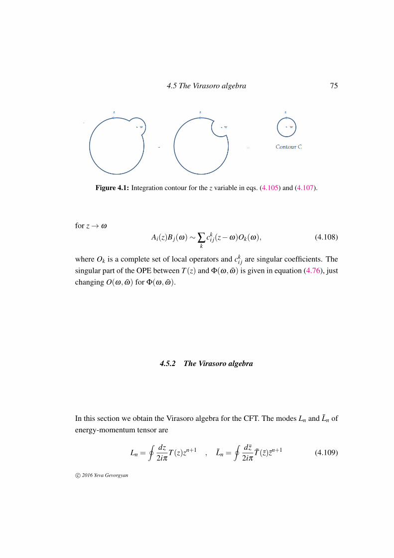
4.5 The Virasoro algebra 75
Figure 4.1: Integration contour for the z variable in eqs. (4.105) and (4.107).
for z→ ω
Ai(z)B j(ω)∼∑k
cki j(z−ω)Ok(ω), (4.108)
where Ok is a complete set of local operators and cki j are singular coefficients. The
singular part of the OPE between T (z) and Φ(ω, ω) is given in equation (4.76), justchanging O(ω, ω) for Φ(ω, ω).
4.5.2 The Virasoro algebra
In this section we obtain the Virasoro algebra for the CFT. The modes Ln and Ln ofenergy-momentum tensor are
Ln =∮ dz
2iπT (z)zn+1 , Ln =
∮ dz2iπ
T (z)zn+1 (4.109)
c© 2016 Yeva Gevorgyan
76 Conformal field theory and strings
If we use radial ordering and equation (4.83), we will obtain the following algebra
[Ln,Lm] =∮
c0
dω
2iπ
∮cω
dz2iπ
ωn+1zm+1R(T (z)T (ω)) =
=∮
c0
dω
2iπ
∮cω
dz2iπ
ωn+1zm+1
(c/2
(z−ω)4 +2T (ω)
(z−ω)2 +∂T (ω)
(z−ω)
)=∮
c0
dω
2iπω
n+1(∮
cω
dz2iπ
zm+1c/2(z−ω)4 +
∮cω
dz2iπ
zm+12T (ω)
(z−ω)2
+∮
cω
dz2iπ
zm+1∂T (ω)
z−ω
)=∮
c0
dω
2iπω
n+1( c
12(m+1)m(m−1)ωm−2 +2(m+1)ωmT (ω)
+ ωm+1
∂ωT (ω))
=c
12(m3−m)
∮c0
ωm+n−1dω
2iπ+2(m+1)
∮c0
dω
2iπTωω
m+n+1
+∮
c0
dω
2iπω
m+n+2∂ωT (ω)
=c
12(m3−m)δm+n +2(m+1)Lm+n
−∮
c0
dω
2iπ(m+n+2)ωm+n+1T (ω)
=c
12(m3−m)δm+n +2(m+1)Lm+n− (m+n+2)Lm+n
=c
12(m3−m)δm+n +(m−n)Lm+n.
(4.110)
Ln modes satisfy the same algebra, and [Ln, Ln] = 0. This is the Virasoro algebra.And every CFT defines a representation of this algebra, depending on central chargec. The central charge part is due to the Weyl rescaling, not to reparametrisation aswe could think.
c© 2016 Yeva Gevorgyan
4.5 The Virasoro algebra 77
4.5.3 Representation of the Virasoro algebra
Let us suppose we have a state |ψ〉, that is an eigenstate of L0 and L0
L0|ψ〉= h|ψ〉, L0|ψ〉= h|ψ〉. (4.111)
By acting with the Ln operator we can get further states with eigenvalues
L0Ln|ψ〉= (LnL0−nLn)|ψ〉= (h−n)Ln|ψ〉, (4.112)
so the Ln are rasing and lowering operators depending on the sign of n. Then n > 0,Ln is lowering and L−n rasing operator. If the spectrum is bounded below whereshould be some states annihilated by all Ln and Ln for n > 0. Such states are calledprimary or highest weight states
Ln|ψ〉= Ln|ψ〉= 0 for all n > 0. (4.113)
This states are the states of lowest energy. So we can now built the Virasoroalgebra by acting on the primary states with raising operators L−n with n > 0. Thestates obtained like this are called descendants. The whole set of states is called aVerna module. They are the irreducible representations of the Virasoro algebra. Soknowing the primary states spectrum brings us to knowing the spectrum of wholetheory. For the vacuum state |0〉= h = 0
Ln|0〉= 0 for all n > 0. (4.114)
This state preserves the maximum number of symmetries. Central charge term inVirasoro algebra does not allow us to have Ln|0〉 = 0 for all n. The states in theVerma module do not need to be all independent. Some linear combinations ofthem can vanish. These linear combinations are called null states. They appeardepending on values of h and c.
c© 2016 Yeva Gevorgyan

78 Conformal field theory and strings
4.5.4 Unitarity of the theory
To be consistent the theory should be unitary. This means that probabilities areconserved in Minkovski signature space-time. Let us take a glance on Hamiltoniandensity
H = Tωω +Tωω = ∑n
Lne−inσ++ Lne−inσ−. (4.115)
So for the Hamiltonian to be Hermitian, we require
Ln = L+−n. (4.116)
We get some strong constraints on the structure of CFTs. Here are some of them
• h > 0: to prove this we write down the norm
|L−1|ψ〉|2 = 〈ψ|L+1L−1|ψ〉= 〈ψ|[L+1,L−1]|ψ〉= 2h〈ψ|ψ〉> 0 (4.117)
the only state with h = 0 is the vacuum state |ψ〉.
• c > 0 : to see this we look at
|L−n|0〉|2 = 〈0|[Ln,L−n]|0〉=c
12n(n2−1)> 0 (4.118)
this gives c > 0. If c = 0 the only state in the vacuum module is the vacuumitself. The vacuum is also the only state in the whole theory.
c© 2016 Yeva Gevorgyan
5
The Fadeev-Popov method and the BRST symmetry
In this chapter we describe the Fadeev-Popov method devised to quantise the Polyakovbosonic action by the path integral method and the BRST (Becchi-Rouet-Stora-Tyutin) symmetry that can also be used to quantise the bosonic string. We limitourselves to the description of the BRST symmetry; we do not quantise the bosonicstring by the BRST method. References for this chapter are [11, 12, 14].
5.1 The path integral
In Euclidean space, the Polyakov action, first introduced by Polyakov in 1981 [16],is given by
SP =− 14πα ′
∫d2
σ√−ggαβ
∂αX µ∂β Xν
δµν , (5.1)
where the integration is over all worldsheet metrics gαβ and all embedding coordi-nates X µ . The corresponding path integral is
Z =∫
Dgαβ (σ ,τ)DX µ(σ ,τ)exp(iSP[X ,g]
). (5.2)
Because of the gauge invariance, the integral is not well defined. This comes fromintegrating infinitely many times over field configurations related by gauge transfor-mations, which are physically equivalent configurations. To turn (5.2) into a welldefined path integral we have to split the integration over all field configurations intotwo pieces corresponding, respectively, to physically distinct configurations and togauge transformations. More explicitly, if we divide the original path integral (5.2)by the infinite volumes of its symmetry groups, we remove the degeneracy factor
79
80 The Fadeev-Popov method and the BRST symmetry
due to the gauge transformations. For the Polyakov action there are two types ofgauge symmetries:
Diffeomorphismsσ
α → σ′α(σα), (5.3)
under which
gαβ (σ)→ g′αβ
(σ ′) =∂σ γ
∂σ ′α∂σδ
∂σ ′βgγδ (σ), (5.4)
Weyl transformationsσ
α → σα , (5.5)
under whichgαβ (σ)→Ω(σ)gαβ (σ). (5.6)
We have thus two symmetry groups, and so two infinite volumes VDiff andVWeyl. With the last argument the path integral becomes
Z′ =1
VDiffVWeyl
∫Dgαβ (σ ,τ)DX µ(σ ,τ)exp
(iSP[X ,g]
). (5.7)
To decompose our integration variables into physical fields and gauge orbits weneed to find the associated Jacobian of the change of variables. The standard methodto do this was first introduced by Fadeev and Popov in a nearly unintelligible 2 pagespaper [17]. The method works for all types of gauge symmetries.
5.1.1 The Faddeev-Popov method
To describe the so called Faddeev-Popov method of finding the Jacobian, we schemat-ically denote both gauge symmetries mentioned before by ζ . The change of themetric under a general transformation is g→ gζ . This is shorthand for
gαβ (σ)→ gζ
αβ(σ ′) = exp
(2ω(σ)
) ∂σ γ
∂σ ′α∂σδ
∂σ ′βgγδ (σ). (5.8)
c© 2016 Yeva Gevorgyan
5.1 The path integral 81
In two dimensions we can put the metric into any form, let us say g, which repre-sents our choice of gauge fixing. But for 2d metric we have some problems:
• We cannot put any 2d metric into the g form we want, we can do this onlylocally. Globally, it is true only for the worldsheet that has the topology of acylinder or a sphere, but not for higher genus surfaces.
• Fixing the metric locally does not fix all the gauge symmetries—conformalsymmetries are still present.
Our goal is to integrate over all physically inequivalent configurations. Let usfirst consider the integral over the gauge orbit of g. For some value of ζ , theconfiguration gζ will be the same as the original metric g. If we put a delta functionin the integral we will have ∫
Dζ δ (g− gζ ) =1
∆FP[g], (5.9)
which is not equal to one because of the Jacobian factor. The Jacobian factor isthe ∆
−1FP[g], and its inverse ∆FP is called the Faddeev-Popov determinant. There are
some facts that we should remember. First, all this procedure is formal and possessthe same difficulties of the path integral approach. Second, we assume that ourgauge fixing is good, and we do not have physically equivalent configurations. Theintegral over gauge transformations Dζ meets only once with the delta function(means that we integrate only ones through every distinct configuration), such thatwe do not have discrete ambiguities (copies of QCD). Finally, the measure is analo-gous to the Haar measure for Lie groups, namely, it is invariant under left and rightactions
Dζ = D(ζ ′ζ ) = D(ζ ζ′). (5.10)
Let us carry out the Faddeev-Popov procedure. We first insert the factor of unityinto the path integral
1 = ∆FP[g]∫
Dζ δ (g− gζ ). (5.11)
c© 2016 Yeva Gevorgyan

82 The Fadeev-Popov method and the BRST symmetry
We call the new path integral Z[g] since it depends on the choice of g:
Z[g] =1
VDiffVWeyl
∫DζDXDg∆FP[g]δ (g− gζ )exp
(−SP[X ,g]
)=
1VDiffVWeyl
∫DζDX∆FP[gζ ]exp
(−SP[X , gζ ]
)=
1VDiffVWeyl
∫DζDX∆FP[g]exp
(−SP[X , g]
).
(5.12)
In the last line we use that the action and the Faddeev-Popov determinant are gaugeinvariant.(1) Now nothing depends on ζ , so the integral over it cancels with thevolumes and we get
Z[g] =∫
DX∆FP[g]exp(−SP[X , g]
). (5.13)
This is the integral over physically inequivalent configurations. The Faddeev-Popovdeterminant is indeed the Jacobian factor that we need.
5.1.2 The Faddeev-Popov determinant
Now we need to compute ∆FP[g] defined as∫Dζ δ (g− gζ ) = ∆
−1FP[g]. (5.14)
Let us assume that the delta function δ (g− gζ ) is non-zero when ζ = 0. Weparameterize the infinitesimal Weyl transformation by ω(σ) and the infinitesimaldiffeomorphism by δσα = vα(0). With these definitions the change in the metric iswritten as
gαβ = 2ω hαβ +∇αvβ +∇β vα . (5.15)
(1)Proof: ∆−1FP [g
ζ ] =∫
ζ′δ (gζ − gζ ′) =
∫ζ′δ (g− gζ−1ζ ′) =
∫ζ′′δ (g− gζ ′′) = ∆
−1FP [g], where we
use the fact that the measure is invariant.
c© 2016 Yeva Gevorgyan
5.1 The path integral 83
Using the last formulae we get
∆−1FP[g] =
∫Dζ (2ω gαβ +∇αvβ +∇β vα). (5.16)
Since we are near the identity we can replace the integral∫
Dζ over the gauge groupwith the integral
∫DωDv over the Lie algebra group and get
∆−1FP[g] =
∫DωDv(2ω gαβ +∇αvβ +∇β vα). (5.17)
Now, by analogy with the Fourier representation of the delta function,
δ (x) =∫
d pe2πipx,
we can insert a “delta functional” into the former functional integral to get
∆−1FP[g] =
∫DωDvDβ exp
(2πi
∫d2
σ√
gβαβ [2ω gαβ +∇αvβ +∇β vα ]
), (5.18)
where β αβ is a symmetric traceless 2-tensor field on the worldsheet, β αβ gαβ = 0,since the integral over ω has to be non-zero (it comes with derivatives). Finally weget
∆−1FP[g] =
∫DvDβ exp
(4πi
∫d2
σ√
gβαβ
∇αvβ
). (5.19)
We got the ∆−1FP , now we want to get ∆FP. To invert the path integral we just need to
go from all bosonic variables to fermionic (Grassmann) variables
βαβ → bαβ ,
vα → cα ,(5.20)
where b and c are anticommuting Grassmann-valued fields. These fields are calledghost fields. With these variables we get for the Faddeev-Popov determinant theexpression
∆FP[g] =∫
DbDcexp(4πi
∫d2
σ√
gbαβ ∇αcβ). (5.21)
c© 2016 Yeva Gevorgyan
84 The Fadeev-Popov method and the BRST symmetry
We define the ghost action as
Sghost =1
2π
∫d2
σ√
gbαβ ∇αcβ , (5.22)
with this definition and rescaling of c and b, we get
∆FP[g] =∫
DbDcexp[iSghost]. (5.23)
In Euclidean space
∆FP[g] =∫
DbDcexp[−Sghost]. (5.24)
By putting equation (5.24) in equation (5.13) we find
Z[g] =∫
DXDbDcexp(−SP[X , g]−Sghost[b,c, g]). (5.25)
So from gauge fixing we got extra ghost fields. This ghost fields are to cancel theunphysical gauge degrees of freedom, and we are left with D−2 transverse modesof X µ . Lorentz invariance is preserved in this type of quantisation. Now let ussimplify the ghost action. In the conformal gauge
gαβ = e2ωδαβ , (5.26)
and the determinant is √g = e2ω . (5.27)
In complex coordinates, the measure is
d2σ =
12
d2z (5.28)
and∇
z = gzz∇z = 2e−2ω
∇z. (5.29)
c© 2016 Yeva Gevorgyan

5.2 The ghost CFT 85
bzz = 0 because bαβ is traceless. So the ghost action is
Sghost =1
2π
∫ 12
d2ze2ω(bzz +bzz)(∇z +∇
z)(cz + cz) =
=1
2π
∫d2z(bzz +bzz)(∇
z +∇z)(cz + cz) =
=1
2π
∫d2z(bzz∇zcz +bzz∇zcz).
(5.30)
We know that∇zcz = ∂zcz +Γ
zzαcα , (5.31)
where the Christoffel symbols are
Γzzα =
12
gzz(∂zgα z +∂αgzz−∂zgzα) = 0 for α = z, z. (5.32)
So the covariant derivative is just an ordinary derivative
∇zcz = ∂zcz, (5.33)
which gives
Sghost =1
2π
∫d2z(bzz∂zcz +bzz∂zcz). (5.34)
At the end we get two free theories. The ghosts are Weyl invariant since they do notdepend on ω .
5.2 The ghost CFT
b and c are anticommuting Grassmann variables. Their dynamics is a subject ofCFT, we will prove this later. If we define them as
b = bzz, b = bzz
c = cz, c = cz.(5.35)
c© 2016 Yeva Gevorgyan
86 The Fadeev-Popov method and the BRST symmetry
The ghost action will be
Sghost =1
2π
∫d2z(b∂c+ b∂ c). (5.36)
For the equations of motion we get
∂b = ∂ b = ∂c = ∂ c = 0 (5.37)
so b and c are holomorphic, but b and c are antiholomorphic. In addition we havethe following conditions:
• periodicity condition for the closed string,
b(σ +2π) = b(σ), c(σ +2π) = c(σ);
• boundary conditions for the open string,
b(σ) = b(σ), c = c(σ) for σ = 0,π,
which come from the vanishing of boundaries upon the derivation of theequations of motion.
Now we need to find the stress tensor for the bc ghosts. The derivation is given inthe appendix B.
T = 2(∂c)b+ c∂b, (5.38)
and for antiholomorphic part
T = 2(∂ c)b+ c∂ b. (5.39)
5.2.1 Operator product expansion
Now we will find the OPEs by the path integral method. We will do this just forthe holomorphic piece of CFT. Using the fact that the integral of a total derivative
c© 2016 Yeva Gevorgyan
5.2 The ghost CFT 87
vanishes for the path integral, we can write
∫DbDc
δ
δb(σ)[e−Sghostb(σ ′)]=
∫DbDce−Sghost
[− 1
2π∂c(σ)b(σ ′)+δ (σ −σ
′)
]= 0.
(5.40)Since this is true for any b and c, we have
∂c(σ)b(σ ′) = 2πδ (σ −σ′). (5.41)
From∫DbDc
δ
δc(σ)[e−Sghostc(σ ′)]=
∫DbDce−Sghost
[− 1
2π∂b(σ)c(σ ′)+δ (σ −σ
′)
]= 0.
(5.42)in the same way we get
∂b(σ)c(σ ′) = 2πδ (σ −σ′). (5.43)
Integrating both equations using the formula ∂ (1/z) = 2πδ (z, z), we find OPEsbetween the ghost fields
b(z)c(ω) =1
z−ω+ · · ·
c(ω)b(z) =1
ω− z+ · · ·
(5.44)
The OPEs of b(z)b(ω) and c(z)c(ω) have no singular parts and vanish as z→ ω .The normal ordered stress-energy tensor of the theory is
T (z) = 2 : ∂c(z)b(z) : + : c(z)∂b(z) :
5.2.2 Primary fields
Here we show that b and c are primary fields, with weights h = 2 and h = −1respectively. To see this we compute OPEs with the stress-energy tensor. For the c
c© 2016 Yeva Gevorgyan
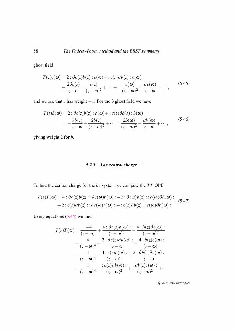
88 The Fadeev-Popov method and the BRST symmetry
ghost field
T (z)c(ω) = 2 : ∂c(z)b(z) : c(ω)+ : c(z)∂b(z) : c(ω) =
=2∂c(z)z−ω
− c(z)(z−ω)2 + · · ·=−
c(ω)
(z−ω)2 +∂c(ω)
z−ω+ · · · ,
(5.45)
and we see that c has weight −1. For the b ghost field we have
T (z)b(ω) = 2 : ∂c(z)b(z) : b(ω)+ : c(z)∂b(z) : b(ω) =
=−∂b(z)z−ω
+2b(z)
(z−ω)2 + · · ·=2b(ω)
(z−ω)2 +∂b(ω)
z−ω+ · · · ,
(5.46)
giving weight 2 for b.
5.2.3 The central charge
To find the central charge for the bc system we compute the T T OPE
T (z)T (ω) = 4 : ∂c(z)b(z) : : ∂c(ω)b(ω) : +2 : ∂c(z)b(z) : : c(ω)∂b(ω) :
+2 : c(z)∂b(z) : : ∂c(ω)b(ω) : + : c(z)∂b(z) : : c(ω)∂b(ω) :(5.47)
Using equations (5.44) we find
T (z)T (ω) =−4
(z−ω)4 +4 : ∂c(z)b(ω) :
(z−ω)2 − 4 : b(z)∂c(ω) :(z−ω)2
− 4(z−ω)4 +
2 : ∂c(z)∂b(ω) :z−ω
− 4 : b(z)c(ω) :(z−ω)3
− 4(z−ω)4 −
4 : c(z)b(ω) :(z−ω)3 +
2 : ∂b(z)∂c(ω) :z−ω
− 1(z−ω)4 −
: c(z)∂b(ω) :(z−ω)2 +
: ∂b(z)c(ω) :(z−ω)2 + · · ·
c© 2016 Yeva Gevorgyan
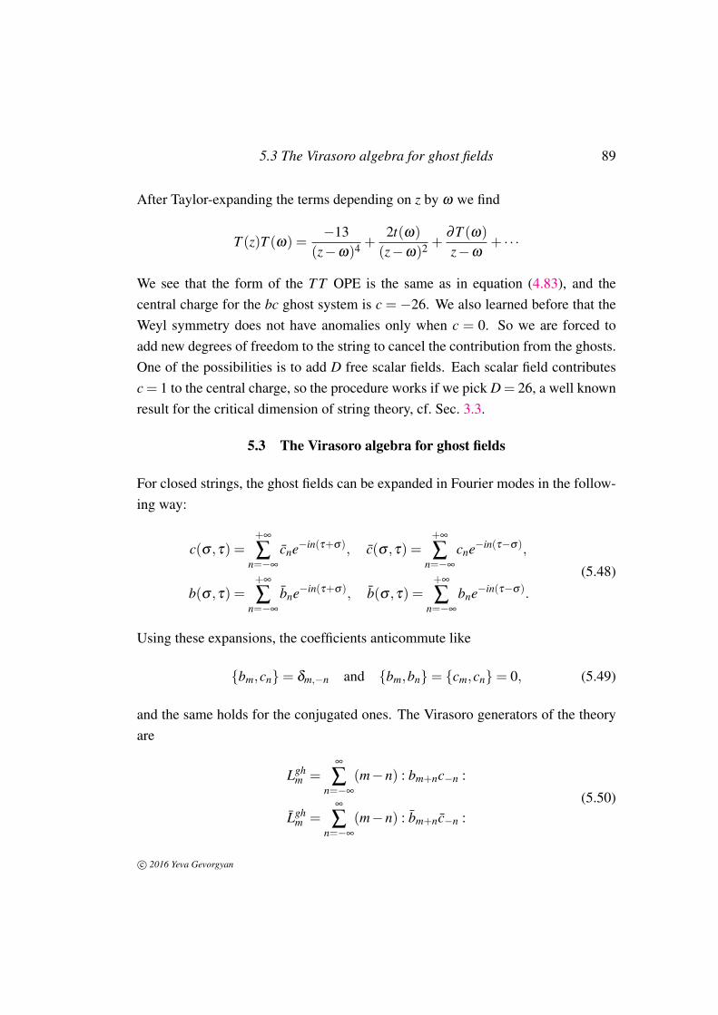
5.3 The Virasoro algebra for ghost fields 89
After Taylor-expanding the terms depending on z by ω we find
T (z)T (ω) =−13
(z−ω)4 +2t(ω)
(z−ω)2 +∂T (ω)
z−ω+ · · ·
We see that the form of the T T OPE is the same as in equation (4.83), and thecentral charge for the bc ghost system is c = −26. We also learned before that theWeyl symmetry does not have anomalies only when c = 0. So we are forced toadd new degrees of freedom to the string to cancel the contribution from the ghosts.One of the possibilities is to add D free scalar fields. Each scalar field contributesc = 1 to the central charge, so the procedure works if we pick D = 26, a well knownresult for the critical dimension of string theory, cf. Sec. 3.3.
5.3 The Virasoro algebra for ghost fields
For closed strings, the ghost fields can be expanded in Fourier modes in the follow-ing way:
c(σ ,τ) =+∞
∑n=−∞
cne−in(τ+σ), c(σ ,τ) =+∞
∑n=−∞
cne−in(τ−σ),
b(σ ,τ) =+∞
∑n=−∞
bne−in(τ+σ), b(σ ,τ) =+∞
∑n=−∞
bne−in(τ−σ).
(5.48)
Using these expansions, the coefficients anticommute like
bm,cn= δm,−n and bm,bn= cm,cn= 0, (5.49)
and the same holds for the conjugated ones. The Virasoro generators of the theoryare
Lghm =
∞
∑n=−∞
(m−n) : bm+nc−n :
Lghm =
∞
∑n=−∞
(m−n) : bm+nc−n :(5.50)
c© 2016 Yeva Gevorgyan
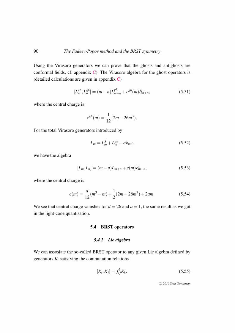
90 The Fadeev-Popov method and the BRST symmetry
Using the Virasoro generators we can prove that the ghosts and antighosts areconformal fields, cf. appendix C). The Virasoro algebra for the ghost operators is(detailed calculations are given in appendix C)
[Lghm ,Lgh
n ] = (m−n)Lghm+n + cgh(m)δm+n, (5.51)
where the central charge is
cgh(m) =1
12(2m−26m3).
For the total Virasoro generators introduced by
Lm = LXm +Lgh
m −aδm,0 (5.52)
we have the algebra
[Lm,Ln] = (m−n)Lm+n + c(m)δm+n, (5.53)
where the central charge is
c(m) =d12
(m3−m)+12(2m−26m3)+2am. (5.54)
We see that central charge vanishes for d = 26 and a = 1, the same result as we gotin the light-cone quantisation.
5.4 BRST operators
5.4.1 Lie algebra
We can assosiate the so-called BRST operator to any given Lie algebra defined bygenerators Ki satisfying the commutation relations
[Ki,K j] = f ki jKk. (5.55)
c© 2016 Yeva Gevorgyan
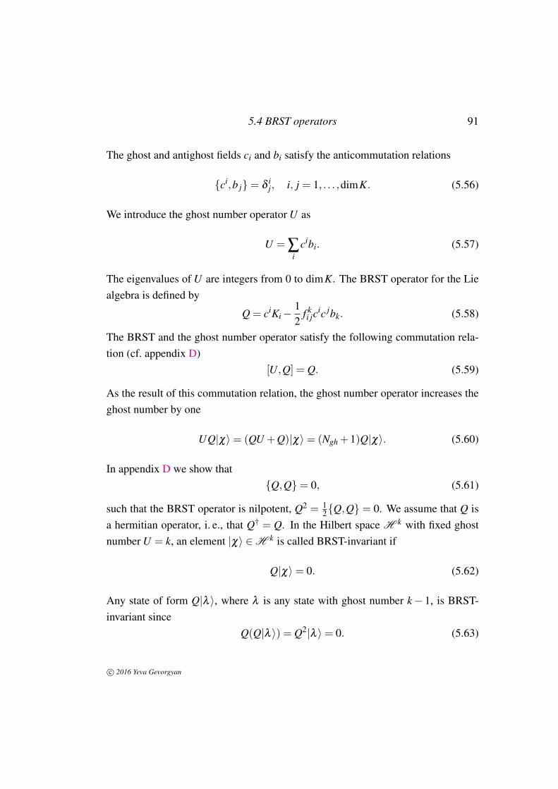
5.4 BRST operators 91
The ghost and antighost fields ci and bi satisfy the anticommutation relations
ci,b j= δij, i, j = 1, . . . ,dimK. (5.56)
We introduce the ghost number operator U as
U = ∑i
cibi. (5.57)
The eigenvalues of U are integers from 0 to dimK. The BRST operator for the Liealgebra is defined by
Q = ciKi−12
f ki jc
ic jbk. (5.58)
The BRST and the ghost number operator satisfy the following commutation rela-tion (cf. appendix D)
[U,Q] = Q. (5.59)
As the result of this commutation relation, the ghost number operator increases theghost number by one
UQ|χ〉= (QU +Q)|χ〉= (Ngh +1)Q|χ〉. (5.60)
In appendix D we show thatQ,Q= 0, (5.61)
such that the BRST operator is nilpotent, Q2 = 12Q,Q = 0. We assume that Q is
a hermitian operator, i. e., that Q† = Q. In the Hilbert space H k with fixed ghostnumber U = k, an element |χ〉 ∈H k is called BRST-invariant if
Q|χ〉= 0. (5.62)
Any state of form Q|λ 〉, where λ is any state with ghost number k− 1, is BRST-invariant since
Q(Q|λ 〉) = Q2|λ 〉= 0. (5.63)
c© 2016 Yeva Gevorgyan
92 The Fadeev-Popov method and the BRST symmetry
We can also see that Q|λ 〉 has zero norm,
〈λ |Q†Q|λ 〉= 〈λ |Q2|λ 〉= 0. (5.64)
Next let us discus states which cannot be presented in the form |χ〉= Q|λ 〉. We saythat two solutions of equation (5.62) are equivalent if
|χ ′〉− |χ〉= Q|λ 〉 (5.65)
for some λ . The states with zero ghost charge should be annihilated by all bk. Forsuch states the BRST operator is
Q = ciKi, so Q|χ〉= ciKi|χ〉= 0, (5.66)
which givesKi|χ〉= 0. (5.67)
This last expression means that |χ〉 is invariant under the action of the Lie algebra.This state cannot be represented as |χ〉= Q|λ 〉 for some λ , because in that case theghost number had to be −1, which is impossible.
5.4.2 The string case
For strings, we take the Lie algebra to be the Virasoro algebra. In addition, we alsohave the ghosts cm and antighosts bm. In this case the BRST operator is given by
Q =+∞
∑−∞
LX−mcm−
12
+∞
∑−∞
(m−n) : c−mc−nbm+n :−ac0, (5.68)
where a is the normal ordering constant for L0. This expression can be written as
Q ==∞
∑−∞
: (LX−m +
12
Lgh−m−aδm,0)cm : (5.69)
c© 2016 Yeva Gevorgyan
5.4 BRST operators 93
The ghost number becomes
U =+∞
∑−∞
: c−mbm : (5.70)
Now let us see what happens with the relation Q2 = 0. We find
Q2 =12Q,Q=
+∞
∑n,m=−∞
([Lm,Ln]− (m−n)Lm+n)c−mc−n, (5.71)
where Lm = LXm + Lgh
m − aδm,0 is a total Virasoro operator. Since the total centralcharge vanishes Q2 = 0 for d = 26 and a = 1. The inverse is also true: from Q2 = 0follows that the central charge of the Virasoro algebra vanishes. First, using (5.49),we see that
Lm = Q,bm. (5.72)
Next
[Lm,Q] = [Q,bm,Q] = (Qbm+bmQ)Q−Q(Qbm+bmQ)= bmQ2−Q2bm = [bm,Q2],
(5.73)as Q2 goes to zero [Lm,Q] also goes to zero. Therefore
[Lm,Ln] = [Lm,Q,bn] = LmQbn +LmbnQ−QbnLm−bnQLm
+LmQbn−QLmbn +LmbnQ−bnLmQ+QLmbn−QbnL+bnLmQ−bnQLm
= [Lm,Q]bn +[Lm,bn]Q+Q[Lm,bn]+bn[Lm,Q] = [Lm,Q],bn+Q, [Lm,bn]= Q, [Lm,bn]= Q,(m−n)bm+n= (m−n)Q,bm+n= (m−n)Lm+n.
(5.74)
In the theory with ghosts we have the new conserved currents
JB = 2c(T X +12
T gh) and J = cb.
c© 2016 Yeva Gevorgyan

94 The Fadeev-Popov method and the BRST symmetry
There is a new fermionic symmetry present, it is a BRST symmetry. The BRSTtransformation is defined as
δY = [λQ,Y ],
where λ is a Grassman (anticomutating) parameter. The explicit transformationsare
δX µ = λc∂X µ +λ c∂X µ , δc = λc∂c, δb = 2λT, and δT = 0. (5.75)
The ghost number operator is
U =12(c0b0−b0c0)+
∞
∑n=1
(c−nbn−b−ncn),
where cn,bn for n > 0 are annihilation operators. For zero-modes we have
c20 = b2
0 = 0, c0,b0= 1.
Or in two dimensions
c0| ↓〉= | ↑〉 b0| ↑〉= | ↓〉c0| ↑〉= 0 b0| ↓〉= 0.
The ghost numbers are U↓ =−12 and U↑ = 1
2 . Physical states should have the ghostnumber −1
2 , so they are annihilated by b0. Indeed cn|ξ 〉 = bn|ξ 〉 = 0 when n > 0and b0|ξ 〉= 0. The condition of BRST invariance becomes
0 = Q|ξ 〉=
(c0(L0−1)+ ∑
n>0c−nLn
)|ξ 〉,
the same as in the case of canonical quantisation. Physical states of the bosonicstring are cohmology classes of the BRST operator with the ghost number −1
2 .
c© 2016 Yeva Gevorgyan

6
Conclusions
In this dissertation we reviewed the Nambu-Goto and Polyakov actions for thebosonic string and quantised these actions covariantly and in the light-cone. Wederived the Virasoro algebra and the Virasoro constraints for the quantum bosonicstring. From the constraints of the theory we could verify that the critical dimensionfor the bosonic string is D = 26. We then analysed the spectrum of a free closedstring and, once again, found that the critical dimension of the bosonic string is D =
26. Some important classical and quantum aspects of two-dimensional conformalfield theories (CFT) that were used to quantise the string by the BRST method werealso analysed, and the Virasoro algebra for the CFT was derived. This allowedus to treat the bosonic string as a two-dimensional CFT. In order to introduce theBRST quantisation procedure for the bosonic string we were led to explore, at apedagogical level, the Faddeev-Popov method of “finding the Jacobian,” the role ofghosts in the theory and their CFT and Virasoro algebra. The introduction of theBRST operators then allowed us to conclude that the physical states should haveghost number −1/2.
The next steps in the study of basic string theory would be to complete theBRST quantisation programme for the bosonic string to the end and then proceedwith the treatment of the fermionic string and superstrings following, for example,the presentations in [10, 14, 18]. Our final goal would be, as per our original project,to understand integrable models related with the quantisation of superstrings onsemisymmetric superspaces [19, 20].
95
96 Conclusions
String theory is a vast subject that employs a diverse set of modern mathemat-ical ideas and techniques. In this dissertation we were able only to start the studyof the techniques that now are classic and belong to the toolbox of almost everytheoretical physicist. We were particularly pleased to learn the basics of CFT andVirasoro algebras. On the other hand, we were not able to start studying anythingabout superstrings, quantum gravity, or the recent developments founded by theAdS/CFT correspondence. Unfortunately, we are not going to pursue this researchprogramme anymore, since we decided to move into another subject.
c© 2016 Yeva Gevorgyan

A
Conservation of the stress-energy tensor
Let us prove that the covariant stress-energy tensor is conserved,
∇αTαβ = 0. (A.1)
The stress-energy tensor is given by
Tαβ = ∂αX µ∂β Xµ −
12
ηαβ ηρσ
∂ρX µ∂σ Xµ . (A.2)
Plugging this expression in (A.1) we get
∇αTαβ = ∇
α∂αX µ
∂β Xµ +∂αX µ∇
α∂β Xµ −
12
∇β ηρσ
∂ρX µ∂σ Xµ . (A.3)
The equation of motion for X µ reads ∇α∂αX µ = 0, so that
∇αTαβ = ∂αX µ
∇α
∂β Xµ −12
∂β ηρσ
∂ρX µ∂σ Xµ =
= ∂αX µη
ασ∇σ ∂β Xµ −
12
∂β ηρσ
∂ρX µ∂σ Xµ −η
ρσ∂ρX µ
∂σ ∂β Xµ =
= ∂αX µη
ασ∂σ ∂β Xµ −∂αX µ
∂λ Xµηασ
Γλ
σβ
− 12
∂β ηρσ
∂ρX µ∂σ Xµ −η
ρσ∂ρX µ
∂σ ∂β Xµ .
(A.4)
97
98 Conservation of the stress-energy tensor
The first and last terms on the right-hand side of the above equation cancel eachother and we are left with
∇αTαβ =−∂αX µ
∂λ Xµηασ
Γλ
σβ− 1
2∂β η
ρσ∂σ X µ
∂σ Xµ . (A.5)
Sinceη
ασΓ
λ
σβ=
12
ηασ
ηλθ
∂σ ηθβ +∂β ηθσ −∂θ ηβσ , (A.6)
the only terms of the above expression that survive the derivatives in (A.5) are theones symmetric in α and λ . Plugging them back into (A.5) furnishes
∇αTαβ =−1
2η
ασ∂β ηθσ η
λθ∂αX µ
∂λ Xµ −12
∂β ηρσ
∂ρX µ∂σ Xµ = 0, (A.7)
that is what we wanted to prove.
c© 2016 Yeva Gevorgyan
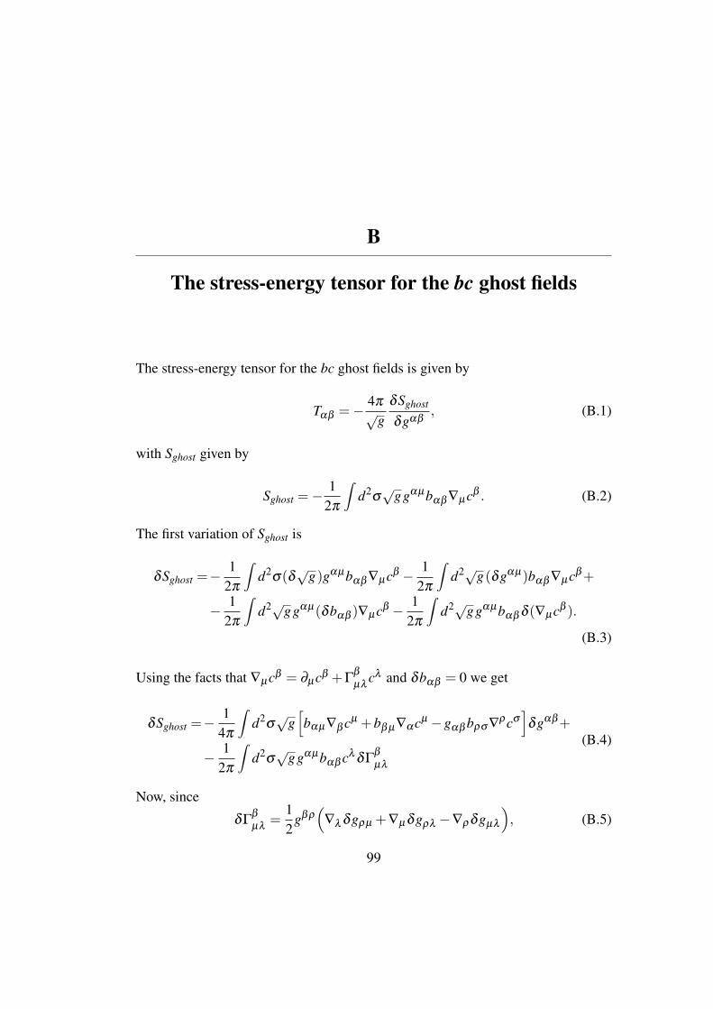
B
The stress-energy tensor for the bc ghost fields
The stress-energy tensor for the bc ghost fields is given by
Tαβ =− 4π√
gδSghost
δgαβ, (B.1)
with Sghost given by
Sghost =−1
2π
∫d2
σ√
ggαµbαβ ∇µcβ . (B.2)
The first variation of Sghost is
δSghost =−1
2π
∫d2
σ(δ√
g)gαµbαβ ∇µcβ − 12π
∫d2√g(δgαµ)bαβ ∇µcβ+
− 12π
∫d2√ggαµ(δbαβ )∇µcβ − 1
2π
∫d2√ggαµbαβ δ (∇µcβ ).
(B.3)
Using the facts that ∇µcβ = ∂µcβ +Γβ
µλcλ and δbαβ = 0 we get
δSghost =−1
4π
∫d2
σ√
g[bαµ∇β cµ +bβ µ∇αcµ −gαβ bρσ ∇
ρcσ
]δgαβ+
− 12π
∫d2
σ√
ggαµbαβ cλδΓ
β
µλ
(B.4)
Now, since
δΓβ
µλ=
12
gβρ
(∇λ δgρµ +∇µδgρλ −∇ρδgµλ
), (B.5)
99

100 The stress-energy tensor for the bc ghost fields
the last term on the right-hand side of (B.4) becomes (note that δΓβ
µλis a tensor)
− 12π
∫d2
σ√
ggαµbαβ cλδΓ
β
µλ=
=− 14π
∫d2
σ√
gbµρcλ
(∇λ δgρµ +∇µδgρλ −∇ρδgρλ
)=
=− 14π
∫d2
σ√
gbµρcλ∇λ δgρµ =
=− 14π
∫d2
σ√
g ∇λ
(bαβ cλ
)δgαβ .
(B.6)
On the other hand, in a flat frame
∇λ
(bαβ cλ
)δgαβ = cλ
∂λ
(bαβ
)δgαβ +∂λ cλ
(bαβ δgαβ
), (B.7)
and since bαβ is traceless the second term on the righ-hand side of the aboveexpression vanishes, ∂λ cλ
(bαβ δgαβ
)= 0. The variation of Sghost then becomes
δSghost =−1
4π
∫d2
σ√
g[bαµ∇β cµ +bβ µ∇αcµ
−gαβ bρσ ∇ρcσ + cλ
∂λ
(bαβ
)δgαβ
]δgαβ ,
(B.8)
and from the definition of the stress-energy tensor we find
Tαβ = bαµ∇β cµ +bβ µ∇αcµ −gαβ bρσ ∇ρcσ + cλ
∂λ
(bαβ
)δgαβ . (B.9)
Using that bαβ gαβ = 0 we get
T = 2(∂c)b+ c(∂b), (B.10)
while the anti-holomorphic part reads
T = 2(∂ c)b+ c(∂ b). (B.11)
c© 2016 Yeva Gevorgyan
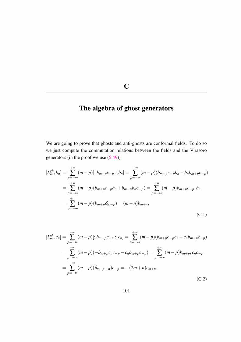
C
The algebra of ghost generators
We are going to prove that ghosts and anti-ghosts are conformal fields. To do sowe just compute the commutation relations between the fields and the Virasorogenerators (in the proof we use (5.49))
[Lghm ,bn] =
+∞
∑p=−∞
(m− p)[: bm+pc−p :,bn] =+∞
∑p=−∞
(m− p)(bm+pc−pbn−bnbm+pc−p)
=+∞
∑p=−∞
(m− p)(bm+pc−pbn +bm+pbnc−p) =+∞
∑p=−∞
(m− p)bm+pc−p,bn
=+∞
∑p=−∞
(m− p)(bm+pδn,−p) = (m−n)bm+n,
(C.1)
[Lghm ,cn] =
+∞
∑p=−∞
(m− p)[: bm+pc−p :,cn] =+∞
∑p=−∞
(m− p)(bm+pc−pcn− cnbm+pc−p)
=+∞
∑p=−∞
(m− p)(−bm+pcnc−p− cnbm+pc−p) =+∞
∑p=−∞
(m− p)bm+p,cnc−p
=+∞
∑p=−∞
(m− p)(δm+p,−n)c−p =−(2m+n)cm+n.
(C.2)
101
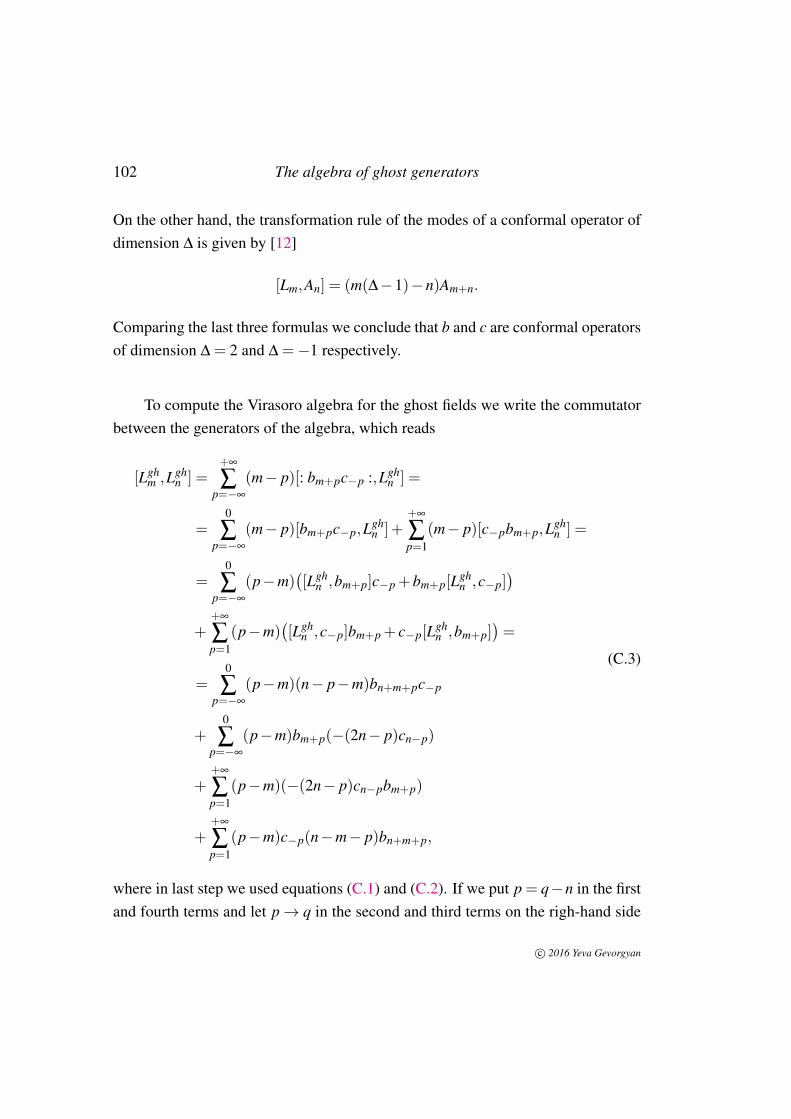
102 The algebra of ghost generators
On the other hand, the transformation rule of the modes of a conformal operator ofdimension ∆ is given by [12]
[Lm,An] = (m(∆−1)−n)Am+n.
Comparing the last three formulas we conclude that b and c are conformal operatorsof dimension ∆ = 2 and ∆ =−1 respectively.
To compute the Virasoro algebra for the ghost fields we write the commutatorbetween the generators of the algebra, which reads
[Lghm ,Lgh
n ] =+∞
∑p=−∞
(m− p)[: bm+pc−p :,Lghn ] =
=0
∑p=−∞
(m− p)[bm+pc−p,Lghn ]+
+∞
∑p=1
(m− p)[c−pbm+p,Lghn ] =
=0
∑p=−∞
(p−m)([Lgh
n ,bm+p]c−p +bm+p[Lghn ,c−p]
)+
+∞
∑p=1
(p−m)([Lgh
n ,c−p]bm+p + c−p[Lghn ,bm+p]
)=
=0
∑p=−∞
(p−m)(n− p−m)bn+m+pc−p
+0
∑p=−∞
(p−m)bm+p(−(2n− p)cn−p)
++∞
∑p=1
(p−m)(−(2n− p)cn−pbm+p)
++∞
∑p=1
(p−m)c−p(n−m− p)bn+m+p,
(C.3)
where in last step we used equations (C.1) and (C.2). If we put p = q−n in the firstand fourth terms and let p→ q in the second and third terms on the righ-hand side
c© 2016 Yeva Gevorgyan
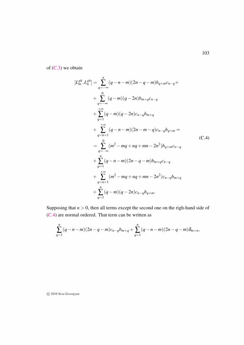
103
of (C.3) we obtain
[Lghm ,Lgh
n ] =n
∑q=−∞
(q−n−m)(2n−q−m)bq+mcn−q+
+0
∑q=−∞
(q−m)(q−2n)bm+qcn−q
++∞
∑q=1
(q−m)(q−2n)cn−qbm+q
++∞
∑q=n+1
(q−n−m)(2n−m−q)cn−qbq+m =
=0
∑q=−∞
(m2−mq+nq+mn−2n2)bq+mcn−q
+n
∑q=1
(q−n−m)(2n−q−m)bm+qcn−q
++∞
∑q=n+1
(m2−mq+nq+mn−2n2)cn−qbm+q
+n
∑q=1
(q−m)(q−2n)cn−qbq+m.
(C.4)
Supposing that n > 0, then all terms except the second one on the righ-hand side of(C.4) are normal ordered. That term can be written as
n
∑q=1
(q−n−m)(2n−q−m)cn−qbm+q +n
∑q=1
(q−n−m)(2n−q−m)δm+n,
c© 2016 Yeva Gevorgyan
104 The algebra of ghost generators
which plugged into (C.4) furnishes
[Lghm ,Lgh
n ] =+∞
∑q=−∞
(m2−mq+nq+mn−2n2) : bm+qcn−q :
+n
∑q=1
(2n−q−m)(q−n−m)δm+n =
=+∞
∑q=−∞
(m−n)(m+n+n−q) : bm+n−n+qc−(q−n) :
+n
∑q=1
(2n−q−m)(q−n−m)δm+n =
= (m−n)Lghm+n +
n
∑q=1
(2n−q−m)(q−n−m)δm+n,
(C.5)
that can then be summed to provide the desired result.
c© 2016 Yeva Gevorgyan
D
Commutation relations between BRSTand ghost number operators
In this appendix we derive some commutation relations between Q, the BRSToperator, and U , the ghost number operator, that were used in this work.
By their definitions,
[Q,U ] = [ciKi−12
f ki jc
iC jBk,Cmbm] =
= ciKicmbm− cmbmciKi−12
f ki jc
ic jbkcmbm +12
f ki jc
mbmcic jbk =
= cicmbmKi− cmbmciKi−12
f ki jc
ic jbkcmbm
− 12
f ki jc
ic jcmbkbm +12
f ki jc
ic jcmbkbm +12
f ki jc
mbmcic jbk =
=−cmci,bmKi−12
f ki jc
ic jbk,cmbm−12
f ki jc
mcic jbmbk +12
f ki jc
mbmcic jbk =
=−cmci,bmKi−12
f ki jc
ic jbk,cmbm−12
f ki jc
m[cic j,bm]bk =
=−cmδ
imKi−
12
f ki jc
ic jδ
mk bm−
12
f ki jc
m(cic j,bm−ci,bmc j)bk =
=−ciKi− 12
f ki jc
ic jbk−12
f ki jc
m(ciδ
mj −δ
mi c j)bk =
=−ciKi− 12
f ki jc
ic jbk−12
f ki jc
jcibk +12
f ki jc
ic jbk =
=−ciKi +12
f ki jc
ic jbk =−Q
(D.1)
105

106Commutation relations between BRST
and ghost number operators
Now let us calculate Q,Q:
Q,Q= ciKi−12
f ki jc
ic jbk,csKs−12
f pmncmcnbp=
= ciKicsKs−12
ciKi f pmncmcnbp−
12
fi jcic jbkcsKs +14
f ki jc
ic jbk f pmncmcnbp
+ csKsciKi−12
csKs f ki jc
ic jbk−12
f pmncmcnbpciKi +
14
f pmncmcnbp f k
i jcic jbk =
= cicsKiKs + csciKsKi−12
f pmncmcncibpKi
− 12
f pmncmcnbpciKi−
12
f ki jc
ic jbkcsKs−12
f ki jc
ic jcsbkKs
+14
f ki j f p
mncic jbkcmcnbp +14
f ki j f p
mncmcnbpcic jbk =
= cicsKiKs + csciKsKi−12
f pmncmcnci,bpKi
− 12
f ki jc
ic jbk,csKs +14
f ki j f p
mncic jbk,cmcnbp
(D.2)
c© 2016 Yeva Gevorgyan
107
The last term is calculated as follows:
f ki j f p
mncic jbk,cmcnbp= f ki j f p
mn(cic jbk,cmcnbp− cic jcmcnbk,bp
+ cmcn[bp,cic j]bk +cmcn,cic jbpbk) =
= f ki j f p
mncic jcm[cn,bk]bp + f ki j f p
mncic jcm,bkcnbp
+ f ki j f p
mncmcnbp,cic jbk− f ki j f p
mncmcncibp,c jbk)
+ f ki j f p
mncmcn,cic jbpbk− f ki j f p
mncmcicn,c jbpbk
+ f ki j f p
mnci[c j,cm]cnbpbk + f ki j f p
mnci,cmc jcnbpbk =
= f ki j f p
mncic jδ
kmcnbp + f k
i j f pmncmcn
δipc jbk− f k
i j f pmncmcnci
δjpbk
+ f ki j f p
mncic jcm[cn,bk]bp + f ki j f p
mnci[c j,cm]cnbpbk
= f ki j f p
mn(cic jcmcnbkbp− cic jcmbkcnbp + cic jcmcnbpbk
− cicmc jcnbpbk + cic jδ
kmcnbp + cmcn
δipc jbk− cmcnci
δjpbk =
=− f ki j f p
mncic jcmδ
nk bp + f k
i j f pmncic j
δkmcnbp
+ f ki j f p
mncmcnδ
ipc jbk− f k
i j f pmncmcnci
δjpbk =
=− f ki j f p
mkcic jcmbp + f ki j f p
kncic jcnbp
+ f ki j f i
mncmcnc jbk− f ki j f j
mncmcncibk =
= 4 f ki j f p
kmcic jcmbp.
(D.3)
Using the above result we obtain
Q,Q= cic j[Ki,K j]−12
f ki jc
ic jKk−12
f ki jc
ic jKk + f ki j f p
kmcic jcmbp, (D.4)
and from the commutation relations for the Ki generators we get
Q,Q= f ki j f p
kmcic jcmbp. (D.5)
c© 2016 Yeva Gevorgyan
108Commutation relations between BRST
and ghost number operators
Due to the anti-commutativity of the ghosts we can write
Q,Q= 13(
f ki j f p
km + f kmi f p
k j + f kjm f p
ki
)cic jcmbp, (D.6)
where the expression inside the parentheses is the Jacobi identity, which is satisfiedby the structure constants of the Lie algebra. This last statement implies that
Q,Q= 0. (D.7)
c© 2016 Yeva Gevorgyan
Bibliography
[1] G. Veneziano, “Construction of a crossing-symmetric, Regge behaved ampli-tude for linearly rising trajectories,” Nuovo Cimento A 57 (1), 190–197 (1968).
[2] J. Wess and B. Zumino, “Supergauge transformations in four dimensions,”Nucl. Phys. B 70 (1), 39–50 (1974).
[3] M. B. Green and J. H. Schwarz, “Anomaly cancellations in supersymmetricD = 10 gauge theory and superstring theory,” Phys. Lett. B 149 (1–3), 117–122 (1984).
[4] D. J. Gross, J. A. Harvey, E. Martinec, and R. Rohm, “Heterotic string,”Phys. Rev. Lett. 54 (6), 502–505 (1985).
[5] E. Witten, “String theory dynamics in various dimensions,” Nucl. Phys. B443 (1), 85–126 (1995).
[6] J. Maldacena, “The large N limit of superconformal field theories andsupergravity,” Int. J. Theor. Phys. 38 (4), 1113–1133 (1999) [arXiv:hep-th/9711200].
[7] O. Aharony, S. S. Gubser, J. M. Maldacena, H. Ooguri, and Y. Oz, “LargeN field theories, string theory and gravity,” Phys. Rep. 323 (3–4), 183–386(2000).
[8] B. Zwiebach, A First Course in String Theory, 2nd ed. (Cambridge:Cambridge University Press, 2009).
109
110 Bibliography
[9] K. Becker, M. Becker, and J. Schwarz, String Theory and M-theory: AModern Introduction (Cambridge: Cambridge University Press, 2007).
[10] M. Green, J. Schwarz, and E. Witten, Superstring Theory, Volume 1:Introduction (Cambridge: Cambridge University Press, 1987).
[11] D. Tong, “Lectures on String Theory (University of Cambridge Part IIIMathematical Tripos),” [arXiv:0908.0333 [hep-th]].
[12] G. Arutyunov, “Lectures on String Theory,” available at http://www.staff.science.uu.nl/~aruty101/.
[13] K. Moriyasu, An Elementary Primer for Gauge Theory (Singapore: WorldScientific, 1983).
[14] J. Polchinsky, String Theory, Volume 1: An Introduction to the Bosonic String(Cambridge: Cambridge University Press, 1998).
[15] L. H. Loomis and S. Sternberg, Advanced Calculus, rev. ed. (Singapore:World Scientific, 2014).
[16] A. M. Polyakov, “Quantum geometry of bosonic strings,” Phys. Lett. B207 (103), 207–210 (1981).
[17] L. D. Faddeev and V. N. Popov, “Feynman diagrams for the Yang-Mills field,”Phys. Lett. B 25 (1), 29–30 (1967).
[18] D. Friedan, E. Martinec, and S. Shenker, “Conformal invariance, supersym-metry and string theory,” Nucl. Phys. B 271 (3–4), 93–165 (1986).
[19] G. Arutyunov and S. Frolov, “Superstrings on AdS(4)×CP3 as a coset sigma-model,” JHEP 2008 (09), art. 129 (26 pp.) (2008) [arXiv:0806.4940 [hep-th]].
[20] K. Zarembo, “Strings on semisymmetric superspaces,” JHEP 2010 (05),art. 002 (23 pp.) (2010) [arXiv:1003.0465 [hep-th]].
c© 2016 Yeva Gevorgyan