Imperial/TP/2012/JS/02

Bosonic Fractionalisation Transitions

Alexander Adam1), Benedict Crampton1), Julian Sonner1),2), Benjamin Withers3)

1)Theoretical Physics Group, Blackett Laboratory,Imperial College, Prince Consort Rd, London SW7 2AZ, U.K.

2)DAMTP, University of Cambridge,C.M.S. Wilberforce Road, Cambridge, CB3 0WA, U.K.

3)Centre for Particle Theory & Department of Mathematical Sciences,

Science Laboratories, South Road, Durham DH1 3LE, U.K.

Abstract

At finite density, charge in holographic systems can be sourced either by

explicit matter sources in the bulk or by bulk horizons. In this paper

we find bosonic solutions of both types, breaking a global U(1) symmetry

in the former case and leaving it unbroken in the latter. Using a minimal

bottom-up model we exhibit phase transitions between the two cases, under

the influence of a relevant operator in the dual field theory. We also embed

solutions and transitions of this type in M-theory, where, holding the theory

at constant chemical potential, the cohesive phase is connected to a neutral

phase of Schrodinger type via a z = 2 QCP .

arX

iv:1

208.

3199

v2 [

hep-

th]

18

Mar

201

3

1 Introduction

Given a holographic system at finite density with respect to some U(1) symmetry, we

would like to answer basic questions relating to the physical nature of its groundstate

such as ‘is the symmetry broken or unbroken?’ and in the latter case ‘are there Fermi

surfaces present?’ and ‘what are the properties of such Fermi surfaces?’. Lately such

questions have attracted a great deal of interest leading to general statements along

the lines of a holographic Luttinger relation and its bosonic analogue [1, 2, 3]. The

Luttinger count relates the sum of the volumes of all Fermi surfaces present to the total

charge, while its bosonic analogue relates the total charge to the ‘Magnus force’ felt

by a test vortex in the dual field theory. Such studies were guided by the realisation

that the finite charge density of a field theory - as encoded in the dual geometry

via a finite electric flux - can be sourced either by explicit charged matter, such as

fermions or charged bosonic condensates, or by a charged horizon. The latter situation

corresponds to having some of the charge density of the field theory tied up in gauge-

variant operators, and correspondingly not contributing to a naively defined Luttinger

count or its bosonic analogue. The charge contributing to this deficit is identified with

so-called ‘fractionalised’ charge in the field theory, that is charge carried by deconfined

‘quark’ degrees of freedom which are charged under the gauge symmetry. This point

of view has recently been bolstered by the identification of the corresponding 2kF

singularities associated with the ‘hidden’ fermionic degrees of freedom by Faulkner and

Iqbal [4].

There can be interesting phase transitions between situations in which flux is sourced

by a horizon to ones where it originates from explicit matter sources in the bulk [1, 5, 6].

An early example of such a transition was observed in the M-theory superconductor [7,

8], where it was demonstrated that the zero-temperature limit of the superconducting

black hole was a charged domain-wall geometry without horizon due to the interplay

of the potential and effective gauge coupling as defined by a neutral scalar field.

The ground states of the Abelian Higgs model with a W-shaped potential were

analysed in [9, 10], where it was observed that the nature of the ground state can

change qualitatively as a function of the gauge coupling. In [7, 8] it was also pointed

out that the disappearance of the horizon as T → 0 can be related to Nernst’s Law since

the charged domain wall has zero entropy, whereas the naive extrapolation of the finite-

temperature geometry to an extremal black hole would carry entropy. It is thus perhaps

expected that the charged domain wall is thermodynamically preferred over the finite-

1

entropy black hole solutions in precisely that region of the phase diagram where both

solutions coexist and thus the ‘entropic singularity’ of the M-theory superconductor is

cloaked by a superconducting dome.

In this work we explore bosonic analogues of the fractionalisation transition of [1],

corresponding to transitions from phases with broken U(1) symmetry to phases with

intact U(1) symmetry and all charge associated with a horizon. The former consti-

tutes the analogue of the ‘mesonic phase1’ of [1] and the latter corresponds to a fully

fractionalised phase. There may also be partially fractionalised phases, in which some

of the charge is carried by the horizon and some by the scalar matter. Because of

the presence of non-singlet matter, the partially fractionalised phase always breaks the

U(1) symmetry, so that the transition between a cohesive and a partially fraction-

alised phase must occur within the superfluid state. Hence we refer to the two kinds

of ordered phases in this paper as the ‘superfluid cohesive phase’ and the ‘superfluid

fractionalised phase’. The transition between the cohesive and fractionalised phase has

striking implications for the full phase diagram (see Fig. 3), yet at this point no field-

theoretical order parameter is known for this transition. We study these transitions in

a variety of models, both in a ‘bottom-up’ and a ‘top-down’ context, with a range of

different behaviours, and we describe the conditions under which fractionalisation tran-

sition can occur. Among other things we describe a supergravity-embedded superfluid

cohesive to neutral phase transition, which has certain aspects that are reminiscent of

the standard superfluid to insulator transition in the Bose-Hubbard model at constant

chemical potential.

It is worth commenting that the theories considered in this paper have a structural

similarity to the Thomas-Fermi approach used in the electron-star literature [12] with

the charged scalar field taking on the role of the fluid of bulk fermions. It should not

come as a surprise then that some of the IR geometries encountered in those studies

will also feature in the bosonic theories here.

An important role is played in the present work by IR geometries with certain scaling

or hyperscaling properties. Such solutions have previously found applications in applied

holography, for example in describing QCD like theories [13, 14, 15], and more recently

in describing quantum-critical matter at finite density [16, 17, 18, 19, 20, 21, 22, 23].

The paper is organised as follows. Immediately following this paragraph we briefly

summarise our results. In section 2 we introduce the class of Einstein-dilaton-charged

1Apart from this one instance we adopt the term ‘cohesive’ for any non-fractionalised phase [11],in order to avoid potential confusions with the more conventional meaning of the term ‘mesonic’.

2

scalar models used throughout the paper and develop their thermodynamics and holo-

graphic renormalisation. Section 3 gives a detailed discussion of certain bottom-up

models which illustrate the general concept of bosonic fractionalisation and motivate

the more subtle M-theory case to which we turn in section 4. We finish with a discussion

and a short appendix.

1.1 Summary of results

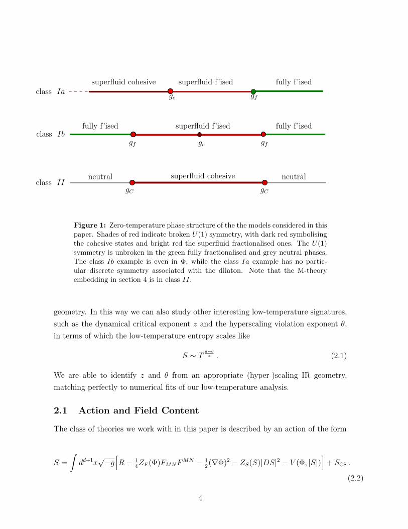
The salient features of the analysis boil down to the IR structure of the zero-temperature

states. We encounter three cases, as illustrated in Fig. 1, depending on the structure

of the effective gauge coupling, which is controlled by the neutral scalar field. If the

gauge coupling vanishes in the IR, we find a fully fractionalised phase, or a superfluid

fractionalised phase. If it remains finite, we find a cohesive phase. The U(1) symmetry

is broken in the latter two phases by explicit charged matter outside the horizon. In ad-

dition to the fully fractionalised phase, there is one further unbroken phase, where the

neutral groundstate does not depend on the chemical potential. This ‘incompressible’

phase together with the transition into it from the cohesive phase via a z = 2 criti-

cal point is reminiscent of the superfluid to insulator transition in the Bose-Hubbard

model.

2 General Features

In this section we introduce the theories leading to quantum phase transitions in terms

of a framework that is general enough to cover both the bottom-up constructions of

section 3 and the M-theory compactifications of section 4. Our general strategy follows

a two-pronged approach. Firstly, at zero temperature we will carry out an analysis of

possible IR geometries and the deformations which allow them to be connected to the

asymptotic AdS configuration universal to all solutions considered in this paper. We

are interested both in IR geometries associated with domain wall configurations and IR

geometries associated with (extremal) black-hole horizons. This allows us to classify

the possible ground states of the holographic theories in this work. Secondly we will

extrapolate the known finite-temperature solutions and their dilatonic deformations

to very low temperatures. These can lead to a state with broken U(1) symmetry via

a condensation instability at some critical temperature Tc or to a state in which this

symmetry is intact. In each case we are able to connect them to the appropriate T = 0

3

class Ia

class Ib

class II

superfluid cohesive

gc gf

superfluid f’ised fully f’ised

neutral superfluid cohesive neutral

fully f’ised superfluid f’ised fully f’ised

gC gC

gf gfgc

Figure 1: Zero-temperature phase structure of the the models considered in thispaper. Shades of red indicate broken U(1) symmetry, with dark red symbolisingthe cohesive states and bright red the superfluid fractionalised ones. The U(1)symmetry is unbroken in the green fully fractionalised and grey neutral phases.The class Ib example is even in Φ, while the class Ia example has no partic-ular discrete symmetry associated with the dilaton. Note that the M-theoryembedding in section 4 is in class II.

geometry. In this way we can also study other interesting low-temperature signatures,

such as the dynamical critical exponent z and the hyperscaling violation exponent θ,

in terms of which the low-temperature entropy scales like

S ∼ Td−θz . (2.1)

We are able to identify z and θ from an appropriate (hyper-)scaling IR geometry,

matching perfectly to numerical fits of our low-temperature analysis.

2.1 Action and Field Content

The class of theories we work with in this paper is described by an action of the form

S =

∫dd+1x

√−g[R− 1

4ZF (Φ)FMNF

MN − 12(∇Φ)2 − ZS(S)|DS|2 − V (Φ, |S|)

]+ SCS .

(2.2)

4

We denote the d+1 bulk directions with upper-case Latin M,N, . . ., whilst field-theory

coordinates will be denoted with lower-case Greek µ, ν, . . .. The field Φ is a neutral

scalar field, which we will refer to as a ‘dilaton’, whereas S is a charged scalar field

with covariant derivative DS = (∇− iqA)S. We have included SCS, which stands for a

possible Chern-Simons or axion-like contribution often found in consistent supergravity

reductions. Whilst the solutions we construct do not depend on SCS, we note that in

certain cases the phase structure may be altered by its presence, for example through

the spontaneous formation of stripes.

We allow the couplings of the gauge field, as well as the charged scalar kinetic

terms, to depend on Φ and S respectively. The interesting transitions observed in the

remainder of this paper can be traced back to the interplay of charged and neutral

scalar couplings and the potential. Often it is convenient to put the scalar kinetic

terms into canonical form. A little thought shows that this is only possible for the

magnitude of the complex field. Writing S in a polar decomposition with phase iqϕ

and then using a field redefinition of the magnitude, we can write the kinetic term of

the charged scalar as

ZS(|S|)|DS|2 = (∇η)2 + q2X(η)2(∇ϕ− A)2 . (2.3)

We should require that X(η) has a small-η expansion X(η) ∼ η +O(η2). The hyper-

scaling geometries are generated by a divergent IR dilaton Φ −→ ±∞, and so it is

important to distinguish theories where such a divergence can happen from those were

it cannot:

class I : ZF (Φ)IR−−−−−→ ∞ ,

class II : ZF (Φ)IR−−−−−→ (always stays bounded) . (2.4)

Furthermore ZF (Φ) may or may not have even symmetry under Φ → −Φ as the

IR limit is approached, again with important implications for the phase structure at

zero temperature. In class I we are particularly interested in ZF (Φ) without this

symmetry, so that e.g. if ZF (Φ) diverges as Φ −→ +∞ then it remains bounded when

Φ diverges with the opposite sign. In this manner the dilaton can naturally drive a

fractionalisation-type phase transition.

Finally we require that the potential has an expansion

`2V (η,Φ) = −6− Φ2 − 2η2 + · · · , (2.5)

5

ensuring that there exists an AdS4 vacuum solution with associated AdS length `2,

and that the two scalars2 Φ and S are dual to ∆ = 2 operators. For the solutions in

this paper we can take the scalar S identically real, so that without loss of generality

ϕ ≡ 0.

Throughout this paper we use the metric ansatz

ds2 = −f(r)e−β(r)dt2 +dr2

f(r)+r2

`2

(dx2 + dy2

). (2.6)

2.2 Holographic renormalisation and asymptotic charges

We are interested in solutions that asymptotically approach the AdS4 fixed point in

the UV. Such solutions admit a large r expansion

f =r2

`2+

1

2

(η2

1 + 12Φ2

1

)+`G1

r+ · · · ,

β = βa +`2(η2

1 + 12Φ2

1

)2r2

+ · · · ,

Φ =`Φ1

r+`2Φ2

r2+ · · · ,

η =`η1

r+`2η2

r2+ · · · ,

At = `e−βa/2(µ− Q

r+ · · ·

). (2.7)

By evaluating the asymptotic stress tensor (which involves introducing counterterms

to render the renormalised expressions finite) we can deduce the exact relationship of

the integration constants introduced here and the physical charges of the dual field

theory. This is achieved by adding the specific counterterm action

Sct = 2

∫∂Σ

√−γ(K − 2

`

)−∫∂Σ

√−γ 1

`

(|S|2 + 1

2Φ2), (2.8)

where we have chosen the counterterms for the scalar fields such that the fixed η1,Φ1

ensemble has a well defined variational principle. K = γµνKµν is the trace of the

extrinsic curvature of a constant r hypersurface with unit normal nr = f(r)12 . We find

that the total action

Sren = S + Sct (2.9)

2The seemingly different mass terms are caused by the different normalisations of the respectivekinetic terms. We are using a convention that appears to be standard in the literature.

6

is finite, as is the renormalised stress tensor

Tµν = 2

[Kµν −Kγµν −

2

`γµν

]− 1

`

(|S|2 + 1

2Φ2)γµν . (2.10)

From this we can relate the expansion coefficient G1 to the energy density3, defined as

ε =reβa

`T00 = −2

`

(G1 − η1η2 − 1

2Φ1Φ2

). (2.11)

The two scalar fields play very different roles in our system. The dilaton Φ gives rise

to an explicit deformation parameter: we switch on a relevant operator by sourcing it

in the dual theory, i.e. by taking a non-zero value of the UV parameter Φ1, and then

study the behaviour of the theory as we vary this source. In contrast, the field η is

only ever allowed to condense spontaneously, i.e. we set η1 = 0.

2.3 Thermodynamic Relations

By analytically continuing to Euclidean signature

t = −iτ , IE = −iSren , (2.12)

we define the grand canonical potential

IE = βΩ(µ, T ) = βvol2ω(µ, T ) . (2.13)

Evaluated on-shell, the action can be written as a total derivative

SOS = iβvol2

∫ ∞r+

d

dr

[2

r

√−ggrr

]dr , (2.14)

which vanishes at the horizon, and thus depends only on the asymptotic charges. Using

techniques of [24, 25] one can show that this is the negative of the pressure

ω(µ, T ) = −P . (2.15)

We can exploit the symmetries of the background metric to derive a Smarr-Gibbs-

Duhem relation. This follows from the vanishing of a certain total derivative4 on shell,

3The quantity e−βa is the boundary speed of light (squared), and so the conversion between ADMmass and energy, and correspondingly energy density, involves a factor of e−βa . For this and relatedreasons it is convenient to set βa = 0, which we will assume to be the case from now on.

4The on-shell vanishing of the total derivative explains why the authors of [8, 24] were able to writethe on-shell action as two different boundary terms.

7

as we now show. By using the Killing equation in addition to the Ricci identity for the

two Killing vectors ∂t and ∂y we can derive the relation

√−g(Rtt −Ry

y

)= −∂r

[e−β/2r2

2`2

(fβ′ − f ′ + 2f

r

)]. (2.16)

It is then a simple matter of using the trace-removed Einstein equations to find that

on-shell√−g(Rtt −Ry

y

)= −1

2∂r[√−gZ(φ)AtF

tr], (2.17)

so that, upon integrating from the horizon to the UV boundary, we obtain the relation

e−β/2r2

`2

(fβ′ − f ′ + 2f

r

)∣∣∣∣∣∞

r+

=√−gZ(φ)AtF

tr∣∣∣∞ . (2.18)

Evaluated on our expansions this gives the Gibbs-Duhem relation

3

2ε = µQ+ Ts− `−1

(η1η2 +

1

2Φ1Φ2

), (2.19)

or, written in terms of the pressure

ε+ P = µQ+ Ts . (2.20)

Here we have used that the temperature is given by

T =e(βa−β+)/2

4π`2f ′(r)

∣∣∣r=r+

, (βa = 0) . (2.21)

Moreover, the entropy density is given in terms of the horizon radius as

s =r2

+

4GN

, (note 16πGN = 1) . (2.22)

The above derivations continue to make sense for solutions of the theory (2.2) where

limr→rIR f′(r) = 0 as rIR → 0, i.e. solutions of vanishing entropy at zero temperature.

We also allow the dilaton field to diverge logarithmically5 in this limit, as long as it

does not interfere with the conditions just mentioned.

5Specifically the dilaton blows up logarithmically as a function of radial proper distance.

8

3 Class I : A Bottom-Up Model

When Z is not symmetric in Φ there is the possibility of two qualitatively different

behaviours assosciated with a dilaton that diverges logarithmically to either plus or

minus infinity. In the following models, we will see that in the first case the effective

gauge coupling e2 ∼ Z−1 will go to zero in the IR and in the second it will diverge. There

is a continuous transition between a superfluid fractionalised phase and a cohesive

phase, via a quantum critical point with a finite dilaton. Both phases will be of

hyperscaling form. This phase transition will be driven by the asymptotic value of the

dilaton. We will also see an additional phase transition between a partially and a fully

fractionalised phase, assosciated with the edge of the superconducting dome.

We will consider the class of models

ZF (Φ) = Z20eaΦ/√

3 , `2V (Φ, η) = −V 20 cosh

(bΦ/√

3)− 2η2 + g2

ηη4 , (3.1)

where a, b > 0. The η4 term allows for interpolating soliton solutions between the AdS4

maximum at η = 0 and the AdS4 minimum at η2 = g−2η . We will study IR geometries

for general values of a and b (see also [1, 11]). All our numerical results will be for the

particular case a = b = g2η = 1, V 2

0 = 6 and Z20 = 1.

3.1 Zero Temperature

We now study the phases of our system at zero temperature. We construct the IR

geometries by making a scaling ansatz for the fields, allowing for a possible logarithmic

divergence of the dilaton. With this divergence the potential is schematically V ∼rδ + r−δ, for some δ, and so these scaling solutions are not exact: they are the leading

order parts of series solutions, with subleading corrections in increasing powers of r.

For each of our three cases we also identify the possible irrelevant deformations.

The divergent dilaton endows our leading order solutions with hyperscaling symme-

try [22, 20, 21], which is a generalisation of the familiar Lifshitz scaling:

x → λx ,

t → λzt ,

r → λ(θ−2)/2r , (3.2)

under which ds → λθ/2ds. Here z is the usual dynamical critical exponent, and θ is

the hyperscaling violation parameter.

9

3.1.1 Fractionalised IR Solutions

In this case some or all of the flux is sourced by the horizon. Starting with the fully

fractionalised case, we switch off the condensate. We find the following scaling solutions

at leading order:

f(r)e−β(r) = r2(12+a2−b2)

(a+b)2 ,

f(r) = f0r2(a−b)a+b ,

At(r) = A0r12+(3a−b)(a+b)

(a+b)2 ,

Φ(r) = − 4√

3

a+ blog r , (3.3)

with

f0 =(a+ b)4V 2

0

4(6 + a(a+ b))(12 + (3a− b)(a+ b)),

A20 =

4(6− b(a+ b))

(12 + (3a− b)(a+ b))Z20

. (3.4)

These solutions have dynamical critical exponent z and hyperscaling parameter θ given

by

z =12 + (a− 3b)(a+ b)

a2 − b2, θ =

4b

b− a. (3.5)

Note that though these parameters are infinite in our special case a = b = 1, their

ratio is still finite (such a situation is discussed further in [11]). This ensures that for

solutions close to this T = 0 geometry, the various thermodynamic parameters have

finite scaling exponents with temperature.

There are two irrelevant deformations about this solution. The first simply corre-

sponds to a shift in the IR vacuum expectation value of the charged scalar:

δη = η0 . (3.6)

Integrating this deformation to the UV gives geometries with explicit bulk charge in

addition to horizon charge. We thus find that the fully fractionalised solutions connect

continuously to the superfluid fractionalised phase branch of solutions. The second

deformation is assosciated with the dilaton, and has the form

δΦ = aIRΦ rνΦ , δf = aIRf rνf , δβ = aIRβ rνΦ , δAt = aIRA rνA , (3.7)

10

with exponents

νf = νΦ +2(a− b)a+ b

,

νA = νΦ +12 + (3a− b)(a+ b)

(a+ b)2, (3.8)

where the coefficients aI and the exponent νΦ are consistently determined by the IR

limit of the linearised equations of motion. For example, in the simplified case a = b

the theory admits an irrelevant deformation with exponent

νΦ =3 + b2

6b4

(−3 +

√81− 24b2

), (3.9)

and coefficients

af , aβ , aA , aΦ = aIR−f0 , 2 ,

A0νΦb2

2(3− b2),− b√

3

, (3.10)

with an overall free magnitude aIR. This is to be compared with the analogous mode

in [1].

3.1.2 Critical IR Solution

The critical IR solution has non-divergent dilaton (in fact Φ = 0) and is just the AdS4

minimum that arises when the condensate sits at the bottom of its potential, η = ±g−1η ,

with vanishing gauge field At(r) = 0. Consequently its AdS length scale is shifted away

from the usual value by a gη-dependent factor:

f(r)e−β(r) = r2 ,

f(r) =r2

R2IR

,

η(r) = ±g−1η , (3.11)

with

R2IR =

6g2η`

2

1 + g2ηV

20

. (3.12)

There are two irrelevant deformations about this solution: one involving the flux and

one the charged condensate. They have the form:

δAt = aIRA rνA , δη = aIRη rνη , (3.13)

11

with exponents

νA =1

2

(−1 +

√1 +

48`2q2

Z20

(1 + g2

ηV2

0

)) ,

νη =3

2

(−1 +

√1 +

32g2η

3(1 + g2

ηV2

0

)) . (3.14)

3.1.3 Cohesive IR Solution

We seek cohesive solutions by demanding that the horizon flux limr→0

√−gZ(Φ)F rt

vanishes. At leading order we find the following scaling solutions and their deforma-

tions:

f(r)e−β(r) = r2 ,

f(r) = f0r2(3−b2)

3 ,

At(r) = 0 ,

Φ(r) =2b√

3log r , (3.15)

with

f0 =3V 2

0

4(9− b2). (3.16)

These solutions have dynamical critical exponent z and hyperscaling parameter θ given

by

z = 1 , θ = − 2b2

3− b2. (3.17)

Just as in the fractionalised case, the vacuum expectation value of the charged scalar

is not fixed, δη = η0. There is then a second irrelevant deformation which introduces

the required flux. For a = b this is

δAt = aIRA r3+b2

6+νA(η0) . (3.18)

This exponent depends on the IR value of the charged scalar:

νA =3 + b2

6

(−2 +

√1 +

72q2η20

Z20f0(3 + b2)2

). (3.19)

This is merely the leading order contribution to the series solution from the deforma-

tion; there are additional subleading corrections in powers of 2νA. We thus have the

12

non-trivial consistency condition that this power be positive, which translates into the

constraint on the condensate:

η20 >

(3 + b2)2f0Z20

24q2. (3.20)

A similar structure was seen in the zero-temperature superconducting solutions of [26].

3.2 Finite Temperature

In order to complement our zero-temperature picture, and to complete our phase dia-

gram, we would like to study how these solutions extend to finite temperature. Holo-

graphically, a non-zero temperature is indicated by the presence of a (non-degenerate)

bulk horizon. We thus make the ansatz

f = f+(r − r+) + · · · ,

β = β+ + · · · ,

At = At,+(r − r+) + · · · ,

Φ = Φ+ + · · · ,

η = η+ + · · · . (3.21)

Temperature masks the singularities of the solutions of section 3.1, and the dilaton

is finite here. Despite this we will see clearly the imprint of the zero temperature

IR scaling behaviour at finite temperature. In particular, our results will exhibit the

striking influence that the quantum critical point has on the finite temperature physics.

Such solutions exhibit a superconducting instability [27, 28], whose critical temper-

ature depends on the value of the dilaton deformation [8]. This critical temperature

can be dialled to zero, forming the edge of a superconducting dome. We have checked

that the free energy of the broken phase solution is lower than that of the unbroken

phase whenever it exists.

Since we are holding the theory at finite chemical potential, it is natural to consider

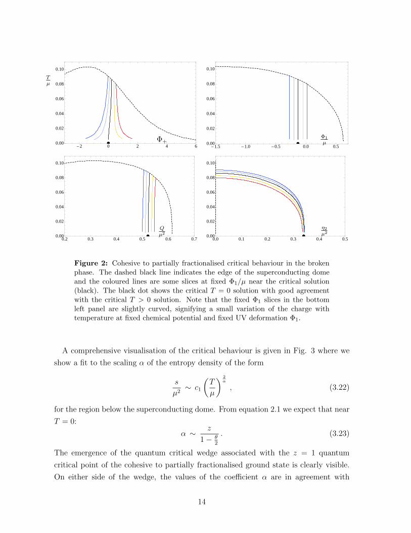
the phase diagram as a function of Φ1/µ. We can illustrate the cohesive to partially

fractionalised critical behaviour at finite T by approaching T = 0 from the top of the

superconducting dome (represented by a black dashed line in each case) at constant

values of Φ1/µ. A selection of such slices is shown in Fig. 2. We see that the critical

solution approaches the unique constant dilaton solution in the IR, while solutions on

either side of it exhibit an IR divergence as T = 0 is approached, consistent with our

earlier analysis.

13

èè-2 0 2 4 6

0.00

0.02

0.04

0.06

0.08

0.10

èè-1.5 -1.0 -0.5 0.0 0.5

0.00

0.02

0.04

0.06

0.08

0.10

èè0.2 0.3 0.4 0.5 0.6 0.70.00

0.02

0.04

0.06

0.08

0.10

èè0.0 0.1 0.2 0.3 0.4 0.50.00

0.02

0.04

0.06

0.08

0.10

Tµ

Φ+Φ1

µ

Qµ2

η2

µ2

Figure 2: Cohesive to partially fractionalised critical behaviour in the brokenphase. The dashed black line indicates the edge of the superconducting domeand the coloured lines are some slices at fixed Φ1/µ near the critical solution(black). The black dot shows the critical T = 0 solution with good agreementwith the critical T > 0 solution. Note that the fixed Φ1 slices in the bottomleft panel are slightly curved, signifying a small variation of the charge withtemperature at fixed chemical potential and fixed UV deformation Φ1.

A comprehensive visualisation of the critical behaviour is given in Fig. 3 where we

show a fit to the scaling α of the entropy density of the form

s

µ2∼ c1

(T

µ

) 2α

, (3.22)

for the region below the superconducting dome. From equation 2.1 we expect that near

T = 0:

α ∼ z

1− θ2

. (3.23)

The emergence of the quantum critical wedge associated with the z = 1 quantum

critical point of the cohesive to partially fractionalised ground state is clearly visible.

On either side of the wedge, the values of the coefficient α are in agreement with

14

the predicted values of α = 2/3 in the cohesive phase and α = 2 in the (partially)

fractionalised phases.

Tµ

Φ1

µ

1.0

0.75

QCP

Figure 3: Scaling behaviour for the quantum-critical region associated with thez = 1, θ = 0 QCP. Colour indicates the value of α, which is proportional to thelogarithmic derivative of entropy with respect to temperature at fixed µ. TheT = 0 QCP is located at the black dot. Hatching indicates low temperatureregions not covered by our data.

3.3 The Fractionalisation Transition

Our analysis thus far can be taken as strong evidence for the existence of a T = 0 phase

transition between a superfluid cohesive phase and a superfluid fractionalised phase at

a critical UV deformation Φ1/µ(gm) ' −0.131. In this section we complete the physical

picture, deforming the IR geometries of section 3.1 by irrelevant deformations in order

to construct full solutions which asymptote to AdS4 in the UV.

Our numerical results are conclusive: we find one-parameter families of full ge-

ometries of each of the three types — superfluid cohesive phase, superfluid fraction-

alised phase and fully fractionalised. The superfluid cohesive phase exists for Φ1/µ <

Φ1/µ(gm). The superfluid fractionalised phase exists for Φ1/µ(gm) < Φ1/µ < Φ1/µ(gf ),

15

meeting the fully fractionalised branch smoothly at Φ1/µ(gf ) ' 0.621.

A holographic measure of fractionalisation is the ratio of flux emanating from the

deep IR of the solution (e.g. a black-hole horizon) and the total charge Q:

AQ≡ 1

Q

(√−gZ(Φ)F rt

∣∣∣r+

). (3.24)

As a consequence of Gauss’s Law, this must interpolate between zero for the superfluid

cohesive phase and unity in the fully fractionalised phase [1, 3, 21]. In Fig. 4 we plot

this measure for each of the solution branches found, which confirms their identities as

either superfluid cohesive, superfluid fractionalised or fully fractionalised.

-0.5 0.0 0.5 1.0

0.0

0.2

0.4

0.6

0.8

1.0

-0.5 0.0 0.5 1.0

-0.20

-0.15

-0.10

-0.05

0.00

AQ

ωµ3

Φ1/µΦ1/µ

gc gfgc

gf

Figure 4: Dependence of the T = 0 domain walls on the parameter Φ1/µ. Asin Fig 1, shades of red indicate broken U(1) symmetry, with dark red indicatinga superfluid cohesive and bright red a superfluid fractionalised phase. Fullyfractionalised geometries are shown in green. Supplementary low temperaturedata (T ' 10−3µ) in the vicinity of the fractionalisation transition gc is indicatedby black dashes.

For the above phase transitions to occur, it is necessary that the fully fractionalised

branch be thermodynamically subdominant wherever it coexists with the superfluid

cohesive or superfluid fractionalised branches. To this end, we plot the free energy

density ω of each family in Fig. 4. We see that the free energy is indeed higher in the

fully fractionalised phase. It proved numerically unprofitable to calculate the T = 0

free energies of the cohesive and superfluid fractionalised branches in a small region

close to the critical point, so in that region we have supplemented our results with low

temperature (T ' 10−3µ) data. Furthermore we note the precise agreement between

the T = 0 analysis and the low temperature results, which is thanks to the plateauing

of the thermodynamic quantities near T = 0 that we (numerically) observed in Fig. 2.

The behaviour of the free energy in Fig. 4 strongly suggests that the phase transition

at gc is continuous. Indeed, we have computed the first two derivatives of the free energy

16

with respect to φ1 and have found them to be continuous about gc, implying at least a

third-order transition. Our supplementary data does not allow us to study arbitrarily

high derivatives with sufficient accuracy.

In contrast, we find a kink in the first derivative of the free energy at gf , implying

a second-order transition there. This tallies well with the fact that, in our model, the

transition at gf is one between a superconducting phase and a normal phase.

Both these results can be compared to the case of fermionic fractionalisation transi-

tions [1], where the roles are reversed. The analogous transition between their ‘mesonic’

(here called ‘cohesive’) and partially fractionalised phases are first or second order, de-

pending on the parameters of the model, while the transition between partial and full

fractionalisation is continuous of third order.

3.4 Class Ib: A Bottom-Up Model

The results we have presented so far map out the detailed phenomenology for a theory

in class Ia, under the classification of Fig. 1, for which the coupling term ZF remains

finite for an interval of UV scalar deformations Φ1. Consequently, we argue, the theory

in this interval was able to support superfluid cohesive solutions which provided the

thermodynamically preferred solutions.

Here we make a few brief comments on a model governed by the same potential

(3.1), but with a Φ-even gauge coupling term ZF (Φ) = Z20 cosh

(aΦ√

3

)with a > 0. The

important feature of this model is that ZF will diverge in the IR given an IR divergent

Φ, irrespective of its sign. Thus, the interval of cohesive solutions exhibited by our

earlier model will here be reduced to a single point, Φ1 = 0. At this point the bulk

solution has Φ(r) = 0 everywhere and is simply an AdS4 to AdS4 charged domain wall.

Thus our model exhibits a transition from superfluid cohesive phase at the point

Φ1 = 0, to superfluid fractionalised phase 0 < |Φ1| < Φ1(gf ), and ultimately to a fully

fractionalised phase when |Φ1| ≥ Φ1(gf ). This is illustrated in Fig 1. We now turn to a

model which arises from a consistent truncation of 11D supergravity, which shares even

gauge coupling Z with class Ib, but which differs from all models in class I by having

finite Z everywhere. As we shall see this leads to markedly different phenomenology.

17

4 M-Theory

We work with the consistent truncation of [8, 29], whose equations of motion can be

obtained from the action

SM =1

16πG

∫d4x√−g[R− (1− h2)3/2

1 + 3h2FMNF

MN − 3

2(1− 34|χ|2)2

|Dχ|2

− 3

2(1− h2)2(∇h)2 − 6

`2

(−1 + h2 + |χ|2)

(1− 34|χ|2)2(1− h2)3/2

]+

1

16πG

∫2h(3 + h2)

1 + 3h2F ∧ F .

(4.1)

By defining χ = ξeiqϕ and performing the transformation

h = tanh

(Φ√3

), ρ =

2√3

tanh

(η√2

), (4.2)

this action falls into the class II of models of (2.2, 2.3) with the specific choices

ZF (Φ) =4

cosh3(

Φ√3

)(1 + 3 tanh2

(Φ√3

)) , X(η) =1√2

sinh(√

2η)

(4.3)

and charge q` = 1, [7]. This model also has a Chern-Simons term. We now turn to

a description of the detailed phase structure of the CFT duals of this system, held at

finite density, with particular regard to the zero-temperature ground states. Much of

this discussion has been reported in the literature [7, 8], and more details can be found

there.

4.1 Phases

As before, a superfluid branch of solutions emerges as an instability of the charged

Reissner-Nordstrom family of solutions which exists in this model when h = 0. Once

again, under the dilaton deformation in the constant µ phase diagram we see a dome of

superconducting solutions, whose T = 0 limit, as shown in [7, 8], is a charged domain

wall interpolating between two AdS regions of different AdS lengths. Whenever the

U(1) symmetry remains unbroken the zero-temperature limit of the neutral and charged

black hole solutions is incompressible, in the sense that it does not depend on the value

of µ. In fact it approaches a zero-density state with vanishing (direct) conductivity.

Furthermore, the T → 0 limit of the neutral and charged solutions meet at the unique,

unbroken T = 0 solution of the system, which lifts to an eleven-dimensional Schrodinger

18

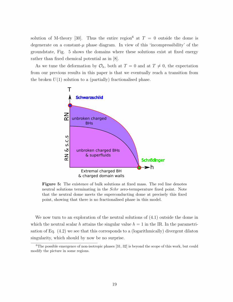
solution of M-theory [30]. Thus the entire region6 at T = 0 outside the dome is

degenerate on a constant-µ phase diagram. In view of this ‘incompressibility’ of the

groundstate, Fig. 5 shows the domains where these solutions exist at fixed energy

rather than fixed chemical potential as in [8].

As we tune the deformation by Oh, both at T = 0 and at T 6= 0, the expectation

from our previous results in this paper is that we eventually reach a transition from

the broken U(1) solution to a (partially) fractionalised phase.

Extremal charged BH& charged domain walls

unbroken charged BHs& superfluids

unbroken chargedBHs

T

h

Schwarzschild

Schrödinger

RN

RN

& s

.c.s

Figure 5: The existence of bulk solutions at fixed mass. The red line denotesneutral solutions terminating in the Schr zero-termperature fixed point. Notethat the neutral dome meets the superconducting dome at precisely this fixedpoint, showing that there is no fractionalised phase in this model.

We now turn to an exploration of the neutral solutions of (4.1) outside the dome in

which the neutral scalar h attains the singular value h = 1 in the IR. In the parametri-

sation of Eq. (4.2) we see that this corresponds to a (logarithmically) divergent dilaton

singularity, which should by now be no surprise.

6The possible emergence of non-isotropic phases [31, 32] is beyond the scope of this work, but couldmodify the picture in some regions.

19

4.2 Neutral top-down solutions

We rewrite (4.1) for the case of interest assuming the charged scalar χ is trivial, since

we do not want solutions in which the U(1) symmetry is broken. Hence, passing to the

variables (4.2), we find

S =

∫d4x√−g[R−

sech3(

Φ√3

)1 + 3 tanh2

(Φ√3

)F 2 − 1

2(∇Φ)2 +

6

`2cosh

(Φ√3

)]. (4.4)

Recall that at finite temperature we have a one-parameter family of neutral ‘dilatonic’

black holes, with IR behaviour (3.21), where ξ ≡ 0. At zero temperature the nature of

the solution changes, as we now describe. Guided by our findings above we suppose7

that the isometries of the metric are enhanced from the R × SO(2) symmetry above

to the full SO(1, 2) Lorentz symmetry. By choosing a convenient radial gauge we take

ds2 =dρ2

F (ρ)+ ρ2sech

(Φ(ρ)/

√3)ηµνdx

µdxν . (4.5)

This expression is convenient for the current purposes, but we note that we can convert

it into the form (2.6) via

r2 = ρ2 sech(

Φ/√

3), e−βf = r2 ,

√F =

dρ

dr

√f . (4.6)

We can use this ansatz to construct the singular IR solutions admitted by the M-theory

truncation.

4.2.1 Singular IR solutions

We can construct the desired IR solution by a standard dimensional reduction trick.

Suppose then that Φ diverges8 in the IR as Φ→∞. In this limit the action approaches

Ssing =

∫d4x√−g[R− 2e−

√3ΦF 2 − 1

2(∇Φ)2 +

3

`2eΦ/√

3], (4.7)

which can be obtained in a reduction via a gravi-photon ansatz

ds2 = eΦ/√

3ds2(M) + e−2Φ/√

3(dz + 2

√2A)2

, (4.8)

7In support of this assumption we have strong numerical evidence for this behaviour by studyingthe zero-temperature approach of the none-extremal black hole solutions.

8The case Φ→ −∞ is equivalent by the Φ→ −Φ symmetry of the lagrangian coming from 11D.

20

where A ∈ T ∗M and hats denote five-dimensional quantities. The starting five-

dimensional action is simply Einstein-Hilbert with a cosmological constant:

S5 =

∫d5x√−g[R +

3

`2

]. (4.9)

Under this reduction, pure five-dimensional AdS with metric

ds25 = `2

5

[dρ2

ρ2+ ρ2

(−dt2 + dx2

)+ ρ2dz2

],

(`2

5 = 4`2), (4.10)

reduces to a logarithmic dilaton solution in four dimensions, that is:

ds2 = `25

[dρ2

ρ+ ρ3(−dt2 + dx2)

], with Φ = −

√3 log(ρ) . (4.11)

This solution, as we shall now see, plays the role of the singular IR we are after. Note

that in this case the gravi-photon field A is trivial, so that the IR solution is obtained

via a simple circle reduction from five dimensions.

Note that we also have a five-dimensional Schrodinger metric [33, 34, 35], obtained

as a simple deformation of the above, by adding a term proportional to the light-cone

coordinate (dx+)2:

ds2 = `25

[−β2ρ4(dx+)2 +

dρ2

ρ2+ ρ2

(dx2

2 + 2dx+dx−)]

, (4.12)

where β is a constant. Once reduced to four dimensions and seen as an expansion

in small ρ, the Schrodinger and AdS metrics in fact agree to leading order, that is

they give the same IR behaviour for the desired logarithmic dilaton solution in four

dimensions. Of course, solving the full equations coming from (4.1) order by order will

determine the exact solution and thus distinguish between the two cases. This was

pointed out earlier in [30].

Here we demonstrate that this solution is in fact the universal T → 0 limit of the

model (4.1) outside the dome. The full M-theory solution, lifted to eleven dimensions,

is a Schrodinger solution Schr5 ×KE6 with dynamical critical exponent z = 2, where

the Schr5 is fibred9 non-trivially over the Kahler-Einstein space KE6. In the dual

field theory this solution corresponds to a mass-deformation driving the system to the

non-relativistic z = 2 IR fixed point [30]. The full structure of this is not evident

from the four-dimensional perspective, but we see the z = 2 scaling for example in the

temperature scaling of entropy density at criticality.

9Similar solutions were constructed previously in [36].

21

Returning thus to constructing the neutral IR solutions, we substitute the metric

ansatz into the equations following from (4.1), resulting in a single, fully decoupled,

non-linear ODE for the scalar field Φ. Its precise form is given in appendix A. Once Φ

is determined, the Einstein equations determine the metric function F (ρ) algebraically:

F (ρ) =4`−2ρ2 cosh

(Φ/√

3)

4− (ρΦ′/√

3)2sech2(Φ/√

3)− 4ρΦ′/

√3 tanh

(Φ/√

3) , (4.13)

where the prime denotes a derivative with respect to the radial direction ρ. The Φ

equation admits an IR expansion, which reproduces (4.11) to leading order. It takes

the form

Φ(ρ) = −√

3 log ρ+3√

3

2ρ2 + · · · , (4.14)

and contains no free parameters. Note that the freedom associated with the ρ rescaling

of the metric has no physical effect on the solution. This unique IR expansion can be

integrated to the UV and connects to the desired skew-whiffed AdS4 solution. We

have done this and read off the UV data. In appropriate units10 one finds h2/h21 =

−0.288 . . . ∼ −1/(2√

3) for the expectation value 〈Oh〉 and ε/h31 = 0.779 . . . ∼ 3

3√

3

for the energy. The analytic values are those of the exact solution found in [8]. One

can check that the chemical potential µ(r∞)− µ(rIR) vanishes. We thus conclude that

the unique neutral T = 0 solution of the theory (4.1) with logarithmically diverging

dilaton is the analytic solution given in Eq (8.2) of [8].

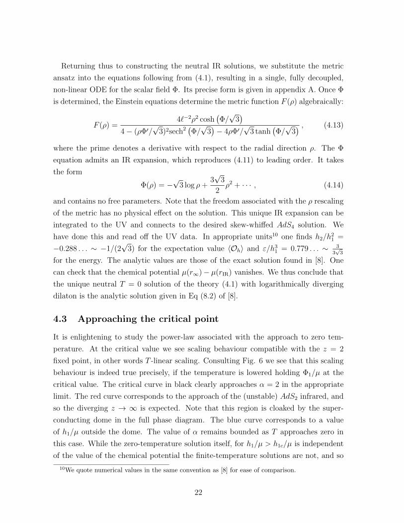
4.3 Approaching the critical point

It is enlightening to study the power-law associated with the approach to zero tem-

perature. At the critical value we see scaling behaviour compatible with the z = 2

fixed point, in other words T -linear scaling. Consulting Fig. 6 we see that this scaling

behaviour is indeed true precisely, if the temperature is lowered holding Φ1/µ at the

critical value. The critical curve in black clearly approaches α = 2 in the appropriate

limit. The red curve corresponds to the approach of the (unstable) AdS2 infrared, and

so the diverging z → ∞ is expected. Note that this region is cloaked by the super-

conducting dome in the full phase diagram. The blue curve corresponds to a value

of h1/µ outside the dome. The value of α remains bounded as T approaches zero in

this case. While the zero-temperature solution itself, for h1/µ > h1c/µ is independent

of the value of the chemical potential the finite-temperature solutions are not, and so

10We quote numerical values in the same convention as [8] for ease of comparison.

22

0.0 0.1 0.2 0.3 0.4 0.5 0.6 0.70

1

2

3

4

5

T/µ

α

Figure 6: Approaching the M-theory Schrodinger critical point from finitetemperature. The black line for h1/µ = h1c/µ = 0.354... shows precisely thecritical T -linear scaling. It delineates the blue supercritical line (h1/µ = 0.382)from the red subcritical line (h1/µ = 0.324). Note that the complex scalar fieldis set to zero in all cases here, and the subcritical region is masked in the fulltheory by a superconducting dome.

the approach does depend on ratios like h1/µ or T/µ. This is clearly illustrated in

Fig. 6, where the critical scaling with α = 2 delineates a region of supercritical (as

exemplified by the blue curve) scaling with α < 2 from a region of subcritical scaling

with α → ∞, as exemplified by the red curve. The latter behaviour corresponds to

approaching the zero-temperature AdS2 geometry, which in the full theory is masked

by the superconducting dome.

5 Discussion

The results of this paper are twofold. On the one hand we have constructed bosonic

analogues of so-called ‘fractionalisation transitions’ by relying on suitably constructed

minimal bottom-up models. On the other hand we reexamined the phase diagram of

the M-theory superconductor in this light, showing how the analogous transition in

this system is in fact a transition from a superfluid cohesive phase to a neutral phase

with vanishing (direct) conductivity11. We emphasise again, that these transitions are

taking place at constant chemical potential.

11Interestingly, however, there is a non-vanishing transverse conductivity Reσxy 6= 0.

23

The IR behaviour of the dilaton coupling to the gauge kinetic term at zero tem-

perature governs the quantum phase transitions observed in this paper. All examples

encountered in this work support the conjecture that one cannot have a cohesive phase

if the dilaton coupling to the gauge-kinetic term diverges (Z →∞). While we do not

have a rigorous argument that would prove this, we can see heuristically that it makes

sense: diverging Z means that the effective gauge coupling vanishes as is obvious in a

normalisation where the gauge-kinetic terms reads ∼ 1e2F 2. That means that matter in

the strict IR, where Z diverges, cannot source any flux. Thus any flux there can only

emanate from a horizon and consequently we would have a fractionalised contribution

to the overall flux. Our arguments for this behaviour are purely holographic, that is

we use the dynamics of the bulk gravity. Similarly our classification of the different

phases are based on such bulk arguments. Clearly it would be very interesting to use

such bulk arguments to shed more light on the nature of a possible order parameter

for the fractionalisation transitions of the kind exemplified in this paper.

In asymptotically AdS spacetimes, one often finds that the zero temperature limit

of a black hole solution has an emergent AdS2 geometry, indicated by a divergent

dynamical critical exponent. The dual field theory then has a non-zero entropy at

zero temperature. Often these finite entropy geometries are unstable when embedded

in top-down models (see e.g. [7, 8, 31]), so that the third law of thermodynamics is

upheld by the classical geometry.

As is clear from equation (2.1), and strikingly visualised in Fig. 3, the T = 0

infared hyperscaling parameter governs the scaling behaviour of various thermodynamic

quantities at low temperature. In particular, a divergent critical exponent can be

compensated for by an equally divergent hyperscaling parameter [11], resulting in a

vanishing entropy at T = 0. In this manner one can avoid instabilities associated

with finite entropy. Our bottom-up model of section 3 uses precisely this mechanism.

The M-theory model, however, is of class II, and so there is no fractionalised phase

associated with a vanishing gauge coupling and its corresponding hyperscaling violation

solutions; we indeed see that the fractionalised (Reisner-Nordstrom) phase is unstable

to scalar condensation, and so masked by a superconducting dome. It would be very

interesting to investigate precisely what conditions have to be met for any entropic

singularity (i.e. any AdS2 IR geometry) to be unstable [37] to new phases cloaking it

at low temperatures.

Recently, following earlier work on Lifshitz geometries [38], it has been suggested

[39, 40] that hyperscaling IR geometries are destabilised due to the running dilaton.

24

If this is the case for the geometries considered here then our results will still apply

for an intermediate range of energy scales, above the scale where quantum corrections

smooth out the IR geometry. It is interesting in this context that at least some of

these seemingly singular geometries can be lifted to perfectly regular higher-dimensional

geometries (see also [22]), potentially eliminating the need to consider the corrections of

[39, 40]. Note, however, that in the case of Lifshitz geometries, the higher-dimensional

lifts were found to be as problematic as their lower-dimensional descendants [41], as

manifested in the propagation of test strings. The status of the possible resolution

of such singularities (e.g. by matter sources [42]) in string theory deserves further

attention.

Acknowledgements

It is a pleasure to thank Aristomenis Donos, Jerome Gauntlett, Andrew Green, Sean

Hartnoll, David Tong and Subir Sachdev for discussions. JS would like to thank the

MCTP at the University of Michigan and the CTP at the Massachusetts Institute of

Technology for hospitality while this work was in progress. AA and BC are supported

by STFC studentships. BW is supported by the Royal Commission for the Exhibition

of 1851.

A The ODE in section 4.2.1

Here we give the details of the ODE determining Φ(ρ) in section 4.2.1, which follows

from the lagrangian (4.7) upon setting At = µ with µ constant.

ρ2Φ′′(ρ) =−1

2√

3tanh

(Φ(ρ)√

3

) [12− ρ2Φ′(ρ)2

(4 + 3 sech2

(Φ(ρ)√

3

))]−[1 + 3 sech2

(Φ(ρ)√

3

)]ρΦ′(ρ) +

1

12sech4

(Φ(ρ)√

3

)ρ3Φ′3(ρ) . (A.1)

For any solution the chemical potential in the boundary theory is arbitrary, as A is

pure gauge in the bulk. If A is to be manifestly well-defined in Kruskal coordinates

one should choose the gauge At = 0.

References

[1] S. A. Hartnoll and L. Huijse, “Fractionalization of holographic Fermi surfaces,”

arXiv:1111.2606 [hep-th].

25

[2] L. Huijse and S. Sachdev, “Fermi surfaces and gauge-gravity duality,” Phys. Rev.

D84 (2011) 026001, arXiv:1104.5022 [hep-th].

[3] N. Iqbal and H. Liu, “Luttinger’s Theorem, Superfluid Vortices, and

Holography,” arXiv:1112.3671 [hep-th]. 21 pages.

[4] T. Faulkner and N. Iqbal, “Friedel oscillations and horizon charge in 1D

holographic liquids,” arXiv:1207.4208 [hep-th].

[5] V. G. M. Puletti, S. Nowling, L. Thorlacius, and T. Zingg, “Holographic metals

at finite temperature,” JHEP 01 (2011) 117, arXiv:1011.6261 [hep-th].

[6] E. D’Hoker and P. Kraus, “Charge Expulsion from Black Brane Horizons, and

Holographic Quantum Criticality in the Plane,” arXiv:1202.2085 [hep-th]. 37

pages v2: reference added and cosmetic improvements.

[7] J. P. Gauntlett, J. Sonner, and T. Wiseman, “Holographic superconductivity in

M-Theory,” Phys. Rev. Lett. 103 (2009) 151601, arXiv:0907.3796 [hep-th].

[8] J. P. Gauntlett, J. Sonner, and T. Wiseman, “Quantum Criticality and

Holographic Superconductors in M- theory,” JHEP 02 (2010) 060,

arXiv:0912.0512 [hep-th].

[9] S. S. Gubser and A. Nellore, “Low-temperature behavior of the Abelian Higgs

model in anti-de Sitter space,” JHEP 0904 (2009) 008, arXiv:0810.4554

[hep-th].

[10] S. S. Gubser and A. Nellore, “Ground states of holographic superconductors,”

Phys. Rev. D80 (2009) 105007, arXiv:0908.1972 [hep-th].

[11] S. A. Hartnoll and E. Shaghoulian, “Spectral weight in holographic scaling

geometries,” arXiv:1203.4236 [hep-th].

[12] S. A. Hartnoll and A. Tavanfar, “Electron stars for holographic metallic

criticality,” Phys.Rev. D83 (2011) 046003, arXiv:1008.2828 [hep-th].

[13] U. Gursoy and E. Kiritsis, “Exploring improved holographic theories for QCD:

Part I,” JHEP 0802 (2008) 032, arXiv:0707.1324 [hep-th].

[14] U. Gursoy, E. Kiritsis, and F. Nitti, “Exploring improved holographic theories

for QCD: Part II,” JHEP 0802 (2008) 019, arXiv:0707.1349 [hep-th].

26

[15] O. DeWolfe, S. S. Gubser, and C. Rosen, “A holographic critical point,”

Phys.Rev. D83 (2011) 086005, arXiv:1012.1864 [hep-th].

[16] M. Taylor, “Non-relativistic holography,” arXiv:0812.0530 [hep-th].

[17] K. Goldstein, S. Kachru, S. Prakash, and S. P. Trivedi, “Holography of Charged

Dilaton Black Holes,” JHEP 1008 (2010) 078, arXiv:0911.3586 [hep-th].

[18] C. Charmousis, B. Gouteraux, B. Kim, E. Kiritsis, and R. Meyer, “Effective

Holographic Theories for low-temperature condensed matter systems,” JHEP

1011 (2010) 151, arXiv:1005.4690 [hep-th].

[19] E. Shaghoulian, “Holographic Entanglement Entropy and Fermi Surfaces,”

JHEP 1205 (2012) 065, arXiv:1112.2702 [hep-th].

[20] N. Ogawa, T. Takayanagi, and T. Ugajin, “Holographic Fermi Surfaces and

Entanglement Entropy,” JHEP 1201 (2012) 125, arXiv:1111.1023 [hep-th].

[21] L. Huijse, S. Sachdev, and B. Swingle, “Hidden Fermi surfaces in compressible

states of gauge-gravity duality,” Phys.Rev. B85 (2012) 035121,

arXiv:1112.0573 [cond-mat.str-el].

[22] B. Gouteraux and E. Kiritsis, “Generalized Holographic Quantum Criticality at

Finite Density,” JHEP 1112 (2011) 036, arXiv:1107.2116 [hep-th].

[23] X. Dong, S. Harrison, S. Kachru, G. Torroba, and H. Wang, “Aspects of

holography for theories with hyperscaling violation,” JHEP 1206 (2012) 041,

arXiv:1201.1905 [hep-th].

[24] J. Sonner and B. Withers, “A gravity derivation of the Tisza-Landau Model in

AdS/CFT,” Phys. Rev. D82 (2010) 026001, arXiv:1004.2707 [hep-th].

[25] J. Bhattacharya, S. Bhattacharyya, S. Minwalla, and A. Yarom, “A theory of

first order dissipative superfluid dynamics,” arXiv:1105.3733 [hep-th].

[26] G. T. Horowitz and M. M. Roberts, “Zero Temperature Limit of Holographic

Superconductors,” JHEP 0911 (2009) 015, arXiv:0908.3677 [hep-th].

[27] S. S. Gubser, “Breaking an Abelian gauge symmetry near a black hole horizon,”

Phys. Rev. D78 (2008) 065034, arXiv:0801.2977 [hep-th].

27

[28] S. A. Hartnoll, C. P. Herzog, and G. T. Horowitz, “Building a Holographic

Superconductor,” Phys. Rev. Lett. 101 (2008) 031601, arXiv:0803.3295

[hep-th].

[29] J. P. Gauntlett, S. Kim, O. Varela, and D. Waldram, “Consistent

supersymmetric Kaluza–Klein truncations with massive modes,” JHEP 04

(2009) 102, arXiv:0901.0676 [hep-th].

[30] H.-C. Kim, S. Kim, K. Lee, and J. Park, “Emergent Schrodinger geometries from

mass-deformed CFT,” JHEP 08 (2011) 111, arXiv:1106.4309 [hep-th].

[31] A. Donos and J. P. Gauntlett, “Holographic striped phases,” JHEP 08 (2011)

140, arXiv:1106.2004 [hep-th].

[32] A. Donos and J. P. Gauntlett, “Holographic helical superconductors,” JHEP 12

(2011) 091, arXiv:1109.3866 [hep-th].

[33] D. Son, “Toward an AdS/cold atoms correspondence: A Geometric realization of

the Schrodinger symmetry,” Phys.Rev. D78 (2008) 046003, arXiv:0804.3972

[hep-th].

[34] K. Balasubramanian and J. McGreevy, “Gravity duals for non-relativistic

CFTs,” Phys.Rev.Lett. 101 (2008) 061601, arXiv:0804.4053 [hep-th].

[35] A. Adams, K. Balasubramanian, and J. McGreevy, “Hot Spacetimes for Cold

Atoms,” JHEP 0811 (2008) 059, arXiv:0807.1111 [hep-th].

[36] E. O Colgain, O. Varela, and H. Yavartanoo, “Non-relativistic M-Theory

solutions based on Kaehler-Einstein spaces,” JHEP 0907 (2009) 081,

arXiv:0906.0261 [hep-th].

[37] N. Iqbal, H. Liu, and M. Mezei, “Quantum phase transitions in semi-local

quantum liquids,” arXiv:1108.0425 [hep-th].

[38] S. Harrison, S. Kachru, and H. Wang, “Resolving Lifshitz Horizons,”

arXiv:1202.6635 [hep-th].

[39] J. Bhattacharya, S. Cremonini, and A. Sinkovics, “On the IR completion of

geometries with hyperscaling violation,” arXiv:1208.1752 [hep-th].

28

[40] N. Kundu, P. Narayan, N. Sircar, and S. P. Trivedi, “Entangled Dilaton Dyons,”

arXiv:1208.2008 [hep-th].

[41] G. T. Horowitz and B. Way, “Lifshitz Singularities,” Phys.Rev. D85 (2012)

046008, arXiv:1111.1243 [hep-th].

[42] N. Bao, X. Dong, S. Harrison, and E. Silverstein, “The Benefits of Stress:

Resolution of the Lifshitz Singularity,” arXiv:1207.0171 [hep-th].

29